Embed Size (px)
Citation preview
gnuplot
An Interactive Plotting Program
Thomas Williams & Colin Kelley
Version 4.3 organized by: Hans-Bernhard Broker, Ethan A Merritt, and others
Major contributors (alphabetic order):Hans-Bernhard Broker
John CampbellRobert Cunningham
David DenholmGershon ElberRoger Fearick
Carsten GrammesLucas Hart
Lars HeckingThomas Koenig
David KotzEd KubaitisRussell Lang
Timothee LecomteAlexander Lehmann
Alexander MaiEthan A Merritt
Petr MikulıkCarsten Steger
Tom TkacikJos Van der Woude
Alex WooJames R. Van Zandt
Johannes ZellnerCopyright c© 1986 - 1993, 1998, 2004 Thomas Williams, Colin Kelley
Copyright c© 2004 - 2007 various authors
Mailing list for comments: [email protected] list for bug reports: [email protected]
Web access (preferred): http://sourceforge.net/projects/gnuplot
This manual was originally prepared by Dick Crawford.
13 June 2008
2 gnuplot 4.3 CONTENTS
Contents
I Gnuplot 15
1 Copyright 15
2 Introduction 15
3 Seeking-assistance 16
4 New features introduced in version 4.3 17
4.1 Internationalization . . . . . . . . . . . . . . . . . . . . . . . . . . . . . . . . . . . . . . . 17
4.2 Transparency . . . . . . . . . . . . . . . . . . . . . . . . . . . . . . . . . . . . . . . . . . . 17
4.3 Volatile Data . . . . . . . . . . . . . . . . . . . . . . . . . . . . . . . . . . . . . . . . . . . 17
4.4 Canvas size . . . . . . . . . . . . . . . . . . . . . . . . . . . . . . . . . . . . . . . . . . . . 17
4.5 New plot elements . . . . . . . . . . . . . . . . . . . . . . . . . . . . . . . . . . . . . . . . 18
4.6 New or revised terminal drivers . . . . . . . . . . . . . . . . . . . . . . . . . . . . . . . . . 18
4.7 New smoothing algorithms . . . . . . . . . . . . . . . . . . . . . . . . . . . . . . . . . . . 18
5 Backwards compatibility 18
6 Batch/Interactive Operation 18
7 Command-line-editing 19
8 Comments 19
9 Coordinates 20
10 Datastrings 20
11 Enhanced text mode 21
12 Environment 22
13 Expressions 23
13.1 Functions . . . . . . . . . . . . . . . . . . . . . . . . . . . . . . . . . . . . . . . . . . . . . 23
13.1.1 Elliptic integrals . . . . . . . . . . . . . . . . . . . . . . . . . . . . . . . . . . . . 25
13.1.2 Random number generator . . . . . . . . . . . . . . . . . . . . . . . . . . . . . . 25
13.2 Operators . . . . . . . . . . . . . . . . . . . . . . . . . . . . . . . . . . . . . . . . . . . . . 26
13.2.1 Unary . . . . . . . . . . . . . . . . . . . . . . . . . . . . . . . . . . . . . . . . . . 26
13.2.2 Binary . . . . . . . . . . . . . . . . . . . . . . . . . . . . . . . . . . . . . . . . . . 26
13.2.3 Ternary . . . . . . . . . . . . . . . . . . . . . . . . . . . . . . . . . . . . . . . . . 27
13.3 Gnuplot-defined variables . . . . . . . . . . . . . . . . . . . . . . . . . . . . . . . . . . . . 27
13.4 User-defined variables and functions . . . . . . . . . . . . . . . . . . . . . . . . . . . . . . 28
14 Glossary 28
CONTENTS gnuplot 4.3 3
15 Linetype, colors, and styles 29
15.1 Colorspec . . . . . . . . . . . . . . . . . . . . . . . . . . . . . . . . . . . . . . . . . . . . . 30
15.1.1 Rgbcolor variable . . . . . . . . . . . . . . . . . . . . . . . . . . . . . . . . . . . . 30
15.1.2 Linecolor variable . . . . . . . . . . . . . . . . . . . . . . . . . . . . . . . . . . . 31
16 Mouse input 31
16.1 Bind . . . . . . . . . . . . . . . . . . . . . . . . . . . . . . . . . . . . . . . . . . . . . . . . 31
16.1.1 Bind space . . . . . . . . . . . . . . . . . . . . . . . . . . . . . . . . . . . . . . . 33
16.2 Mouse variables . . . . . . . . . . . . . . . . . . . . . . . . . . . . . . . . . . . . . . . . . 33
17 Plotting 33
18 Start-up 34
19 String constants and string variables 34
20 Substitution and Command line macros 35
20.1 Substitution of system commands in backquotes . . . . . . . . . . . . . . . . . . . . . . . 35
20.2 Substitution of string variables as macros . . . . . . . . . . . . . . . . . . . . . . . . . . . 35
20.3 String variables, macros, and command line substitution . . . . . . . . . . . . . . . . . . 36
21 Syntax 36
21.1 Quote Marks . . . . . . . . . . . . . . . . . . . . . . . . . . . . . . . . . . . . . . . . . . . 37
22 Time/Date data 37
II Plotting styles 38
23 Boxerrorbars 38
24 Boxes 39
25 Boxxyerrorbars 40
26 Candlesticks 40
27 Circles 41
28 Dots 41
29 Filledcurves 41
30 Financebars 42
31 Fsteps 43
32 Histeps 43
4 gnuplot 4.3 CONTENTS
33 Histograms 43
33.1 Newhistogram . . . . . . . . . . . . . . . . . . . . . . . . . . . . . . . . . . . . . . . . . . 46
33.2 Automated iteration over multiple columns . . . . . . . . . . . . . . . . . . . . . . . . . . 46
34 Image 46
34.1 Transparency . . . . . . . . . . . . . . . . . . . . . . . . . . . . . . . . . . . . . . . . . . . 47
34.2 Image failsafe . . . . . . . . . . . . . . . . . . . . . . . . . . . . . . . . . . . . . . . . . . . 47
35 Impulses 47
36 Labels 47
37 Lines 48
38 Linespoints 48
39 Points 48
40 Steps 49
41 Rgbalpha 49
42 Rgbimage 49
43 Vectors 49
44 Xerrorbars 49
45 Xyerrorbars 50
46 Yerrorbars 50
47 Xerrorlines 50
48 Xyerrorlines 51
49 Yerrorlines 51
50 3D (surface) plots 51
III Commands 52
51 Cd 52
52 Call 53
53 Clear 53
54 Evaluate 53
CONTENTS gnuplot 4.3 5
55 Exit 54
56 Fit 54
56.1 Adjustable parameters . . . . . . . . . . . . . . . . . . . . . . . . . . . . . . . . . . . . . . 55
56.2 Short introduction . . . . . . . . . . . . . . . . . . . . . . . . . . . . . . . . . . . . . . . . 56
56.3 Error estimates . . . . . . . . . . . . . . . . . . . . . . . . . . . . . . . . . . . . . . . . . . 56
56.3.1 Statistical overview . . . . . . . . . . . . . . . . . . . . . . . . . . . . . . . . . . 57
56.3.2 Practical guidelines . . . . . . . . . . . . . . . . . . . . . . . . . . . . . . . . . . 57
56.4 Control . . . . . . . . . . . . . . . . . . . . . . . . . . . . . . . . . . . . . . . . . . . . . . 58
56.4.1 Control variables . . . . . . . . . . . . . . . . . . . . . . . . . . . . . . . . . . . . 58
56.4.2 Environment variables . . . . . . . . . . . . . . . . . . . . . . . . . . . . . . . . . 59
56.5 Multi-branch . . . . . . . . . . . . . . . . . . . . . . . . . . . . . . . . . . . . . . . . . . . 59
56.6 Starting values . . . . . . . . . . . . . . . . . . . . . . . . . . . . . . . . . . . . . . . . . . 59
56.7 Tips . . . . . . . . . . . . . . . . . . . . . . . . . . . . . . . . . . . . . . . . . . . . . . . . 60
57 Help 60
58 History 61
59 If 61
60 Iteration 62
61 Load 62
62 Lower 62
63 Pause 63
64 Plot 63
64.1 Axes . . . . . . . . . . . . . . . . . . . . . . . . . . . . . . . . . . . . . . . . . . . . . . . . 64
64.2 Data . . . . . . . . . . . . . . . . . . . . . . . . . . . . . . . . . . . . . . . . . . . . . . . . 64
64.2.1 Binary . . . . . . . . . . . . . . . . . . . . . . . . . . . . . . . . . . . . . . . . . . 66
64.2.2 Binary general . . . . . . . . . . . . . . . . . . . . . . . . . . . . . . . . . . . . . 66
64.2.2.1 Array . . . . . . . . . . . . . . . . . . . . . . . . . . . . . . . . . . . . 67
64.2.2.2 Record . . . . . . . . . . . . . . . . . . . . . . . . . . . . . . . . . . . 67
64.2.2.3 Skip . . . . . . . . . . . . . . . . . . . . . . . . . . . . . . . . . . . . 67
64.2.2.4 Format . . . . . . . . . . . . . . . . . . . . . . . . . . . . . . . . . . . 67
64.2.2.5 Endian . . . . . . . . . . . . . . . . . . . . . . . . . . . . . . . . . . . 67
64.2.2.6 Filetype . . . . . . . . . . . . . . . . . . . . . . . . . . . . . . . . . . 68
64.2.2.6.1 Avs . . . . . . . . . . . . . . . . . . . . . . . . . . . . . . . . 68
64.2.2.6.2 Edf . . . . . . . . . . . . . . . . . . . . . . . . . . . . . . . . 68
64.2.2.7 Keywords . . . . . . . . . . . . . . . . . . . . . . . . . . . . . . . . . 68
64.2.2.7.1 Scan . . . . . . . . . . . . . . . . . . . . . . . . . . . . . . . 68
64.2.2.7.2 Transpose . . . . . . . . . . . . . . . . . . . . . . . . . . . . 68
6 gnuplot 4.3 CONTENTS
64.2.2.7.3 Dx, dy, dz . . . . . . . . . . . . . . . . . . . . . . . . . . . . 68
64.2.2.7.4 Flipx, flipy, flipz . . . . . . . . . . . . . . . . . . . . . . . . . 68
64.2.2.7.5 Origin . . . . . . . . . . . . . . . . . . . . . . . . . . . . . . 69
64.2.2.7.6 Center . . . . . . . . . . . . . . . . . . . . . . . . . . . . . . 69
64.2.2.7.7 Rotate . . . . . . . . . . . . . . . . . . . . . . . . . . . . . . 69
64.2.2.7.8 Perpendicular . . . . . . . . . . . . . . . . . . . . . . . . . . 69
64.2.2.8 Binary examples . . . . . . . . . . . . . . . . . . . . . . . . . . . . . . 69
64.2.3 Every . . . . . . . . . . . . . . . . . . . . . . . . . . . . . . . . . . . . . . . . . . 70
64.2.4 Example datafile . . . . . . . . . . . . . . . . . . . . . . . . . . . . . . . . . . . . 70
64.2.5 Index . . . . . . . . . . . . . . . . . . . . . . . . . . . . . . . . . . . . . . . . . . 71
64.2.6 Smooth . . . . . . . . . . . . . . . . . . . . . . . . . . . . . . . . . . . . . . . . . 71
64.2.6.1 Acsplines . . . . . . . . . . . . . . . . . . . . . . . . . . . . . . . . . . 72
64.2.6.2 Bezier . . . . . . . . . . . . . . . . . . . . . . . . . . . . . . . . . . . 72
64.2.6.3 Csplines . . . . . . . . . . . . . . . . . . . . . . . . . . . . . . . . . . 72
64.2.6.4 Sbezier . . . . . . . . . . . . . . . . . . . . . . . . . . . . . . . . . . . 72
64.2.6.5 Unique . . . . . . . . . . . . . . . . . . . . . . . . . . . . . . . . . . . 72
64.2.6.6 Frequency . . . . . . . . . . . . . . . . . . . . . . . . . . . . . . . . . 72
64.2.6.7 Cumulative . . . . . . . . . . . . . . . . . . . . . . . . . . . . . . . . 72
64.2.6.8 Kdensity . . . . . . . . . . . . . . . . . . . . . . . . . . . . . . . . . . 73
64.2.7 Special-filenames . . . . . . . . . . . . . . . . . . . . . . . . . . . . . . . . . . . . 73
64.2.8 Thru . . . . . . . . . . . . . . . . . . . . . . . . . . . . . . . . . . . . . . . . . . . 74
64.2.9 Using . . . . . . . . . . . . . . . . . . . . . . . . . . . . . . . . . . . . . . . . . . 74
64.2.9.1 Using examples . . . . . . . . . . . . . . . . . . . . . . . . . . . . . . 75
64.2.9.2 Pseudocolumns . . . . . . . . . . . . . . . . . . . . . . . . . . . . . . 76
64.2.9.3 Using title . . . . . . . . . . . . . . . . . . . . . . . . . . . . . . . . . 76
64.2.9.4 Xticlabels . . . . . . . . . . . . . . . . . . . . . . . . . . . . . . . . . 76
64.2.9.5 X2ticlabels . . . . . . . . . . . . . . . . . . . . . . . . . . . . . . . . . 76
64.2.9.6 Yticlabels . . . . . . . . . . . . . . . . . . . . . . . . . . . . . . . . . 76
64.2.9.7 Y2ticlabels . . . . . . . . . . . . . . . . . . . . . . . . . . . . . . . . . 77
64.2.9.8 Zticlabels . . . . . . . . . . . . . . . . . . . . . . . . . . . . . . . . . 77
64.3 Errorbars . . . . . . . . . . . . . . . . . . . . . . . . . . . . . . . . . . . . . . . . . . . . . 77
64.4 Errorlines . . . . . . . . . . . . . . . . . . . . . . . . . . . . . . . . . . . . . . . . . . . . . 77
64.5 Parametric . . . . . . . . . . . . . . . . . . . . . . . . . . . . . . . . . . . . . . . . . . . . 78
64.6 Ranges . . . . . . . . . . . . . . . . . . . . . . . . . . . . . . . . . . . . . . . . . . . . . . 78
64.7 Iteration . . . . . . . . . . . . . . . . . . . . . . . . . . . . . . . . . . . . . . . . . . . . . 79
64.8 Title . . . . . . . . . . . . . . . . . . . . . . . . . . . . . . . . . . . . . . . . . . . . . . . . 80
64.9 With . . . . . . . . . . . . . . . . . . . . . . . . . . . . . . . . . . . . . . . . . . . . . . . 80
65 Print 82
66 Pwd 83
67 Quit 83
CONTENTS gnuplot 4.3 7
68 Raise 83
69 Refresh 83
70 Replot 83
71 Reread 84
72 Reset 85
73 Save 85
74 Set-show 85
74.1 Angles . . . . . . . . . . . . . . . . . . . . . . . . . . . . . . . . . . . . . . . . . . . . . . . 86
74.2 Arrow . . . . . . . . . . . . . . . . . . . . . . . . . . . . . . . . . . . . . . . . . . . . . . . 86
74.3 Autoscale . . . . . . . . . . . . . . . . . . . . . . . . . . . . . . . . . . . . . . . . . . . . . 88
74.3.1 Parametric mode . . . . . . . . . . . . . . . . . . . . . . . . . . . . . . . . . . . . 89
74.3.2 Polar mode . . . . . . . . . . . . . . . . . . . . . . . . . . . . . . . . . . . . . . . 89
74.4 Bars . . . . . . . . . . . . . . . . . . . . . . . . . . . . . . . . . . . . . . . . . . . . . . . . 90
74.5 Bind . . . . . . . . . . . . . . . . . . . . . . . . . . . . . . . . . . . . . . . . . . . . . . . . 90
74.6 Bmargin . . . . . . . . . . . . . . . . . . . . . . . . . . . . . . . . . . . . . . . . . . . . . 90
74.7 Border . . . . . . . . . . . . . . . . . . . . . . . . . . . . . . . . . . . . . . . . . . . . . . 90
74.8 Boxwidth . . . . . . . . . . . . . . . . . . . . . . . . . . . . . . . . . . . . . . . . . . . . . 91
74.9 Clabel . . . . . . . . . . . . . . . . . . . . . . . . . . . . . . . . . . . . . . . . . . . . . . . 92
74.10 Clip . . . . . . . . . . . . . . . . . . . . . . . . . . . . . . . . . . . . . . . . . . . . . . . . 92
74.11 Cntrparam . . . . . . . . . . . . . . . . . . . . . . . . . . . . . . . . . . . . . . . . . . . . 93
74.12 Color box . . . . . . . . . . . . . . . . . . . . . . . . . . . . . . . . . . . . . . . . . . . . . 94
74.13 Colornames . . . . . . . . . . . . . . . . . . . . . . . . . . . . . . . . . . . . . . . . . . . . 95
74.14 Contour . . . . . . . . . . . . . . . . . . . . . . . . . . . . . . . . . . . . . . . . . . . . . . 95
74.15 Data style . . . . . . . . . . . . . . . . . . . . . . . . . . . . . . . . . . . . . . . . . . . . . 96
74.16 Datafile . . . . . . . . . . . . . . . . . . . . . . . . . . . . . . . . . . . . . . . . . . . . . . 96
74.16.1 Set datafile fortran . . . . . . . . . . . . . . . . . . . . . . . . . . . . . . . . . . . 96
74.16.2 Set datafile nofpe trap . . . . . . . . . . . . . . . . . . . . . . . . . . . . . . . . . 96
74.16.3 Set datafile missing . . . . . . . . . . . . . . . . . . . . . . . . . . . . . . . . . . 96
74.16.4 Set datafile separator . . . . . . . . . . . . . . . . . . . . . . . . . . . . . . . . . 97
74.16.5 Set datafile commentschars . . . . . . . . . . . . . . . . . . . . . . . . . . . . . . 98
74.16.6 Set datafile binary . . . . . . . . . . . . . . . . . . . . . . . . . . . . . . . . . . . 98
74.17 Decimalsign . . . . . . . . . . . . . . . . . . . . . . . . . . . . . . . . . . . . . . . . . . . . 98
74.18 Dgrid3d . . . . . . . . . . . . . . . . . . . . . . . . . . . . . . . . . . . . . . . . . . . . . . 99
74.19 Dummy . . . . . . . . . . . . . . . . . . . . . . . . . . . . . . . . . . . . . . . . . . . . . . 100
74.20 Encoding . . . . . . . . . . . . . . . . . . . . . . . . . . . . . . . . . . . . . . . . . . . . . 101
74.21 Fit . . . . . . . . . . . . . . . . . . . . . . . . . . . . . . . . . . . . . . . . . . . . . . . . . 101
74.22 Fontpath . . . . . . . . . . . . . . . . . . . . . . . . . . . . . . . . . . . . . . . . . . . . . 102
74.23 Format . . . . . . . . . . . . . . . . . . . . . . . . . . . . . . . . . . . . . . . . . . . . . . 102
8 gnuplot 4.3 CONTENTS
74.23.1 Gprintf . . . . . . . . . . . . . . . . . . . . . . . . . . . . . . . . . . . . . . . . . 103
74.23.2 Format specifiers . . . . . . . . . . . . . . . . . . . . . . . . . . . . . . . . . . . . 103
74.23.3 Time/date specifiers . . . . . . . . . . . . . . . . . . . . . . . . . . . . . . . . . . 104
74.24 Function style . . . . . . . . . . . . . . . . . . . . . . . . . . . . . . . . . . . . . . . . . . 105
74.25 Functions . . . . . . . . . . . . . . . . . . . . . . . . . . . . . . . . . . . . . . . . . . . . . 105
74.26 Grid . . . . . . . . . . . . . . . . . . . . . . . . . . . . . . . . . . . . . . . . . . . . . . . . 105
74.27 Hidden3d . . . . . . . . . . . . . . . . . . . . . . . . . . . . . . . . . . . . . . . . . . . . . 106
74.28 Historysize . . . . . . . . . . . . . . . . . . . . . . . . . . . . . . . . . . . . . . . . . . . . 107
74.29 Isosamples . . . . . . . . . . . . . . . . . . . . . . . . . . . . . . . . . . . . . . . . . . . . 108
74.30 Key . . . . . . . . . . . . . . . . . . . . . . . . . . . . . . . . . . . . . . . . . . . . . . . . 108
74.30.1 Key placement . . . . . . . . . . . . . . . . . . . . . . . . . . . . . . . . . . . . . 110
74.30.2 Key samples . . . . . . . . . . . . . . . . . . . . . . . . . . . . . . . . . . . . . . 111
74.31 Label . . . . . . . . . . . . . . . . . . . . . . . . . . . . . . . . . . . . . . . . . . . . . . . 111
74.32 Lmargin . . . . . . . . . . . . . . . . . . . . . . . . . . . . . . . . . . . . . . . . . . . . . . 113
74.33 Loadpath . . . . . . . . . . . . . . . . . . . . . . . . . . . . . . . . . . . . . . . . . . . . . 113
74.34 Locale . . . . . . . . . . . . . . . . . . . . . . . . . . . . . . . . . . . . . . . . . . . . . . . 113
74.35 Logscale . . . . . . . . . . . . . . . . . . . . . . . . . . . . . . . . . . . . . . . . . . . . . . 113
74.36 Macros . . . . . . . . . . . . . . . . . . . . . . . . . . . . . . . . . . . . . . . . . . . . . . 114
74.37 Mapping . . . . . . . . . . . . . . . . . . . . . . . . . . . . . . . . . . . . . . . . . . . . . 114
74.38 Margin . . . . . . . . . . . . . . . . . . . . . . . . . . . . . . . . . . . . . . . . . . . . . . 115
74.39 Mouse . . . . . . . . . . . . . . . . . . . . . . . . . . . . . . . . . . . . . . . . . . . . . . . 115
74.39.1 X11 mouse . . . . . . . . . . . . . . . . . . . . . . . . . . . . . . . . . . . . . . . 116
74.40 Multiplot . . . . . . . . . . . . . . . . . . . . . . . . . . . . . . . . . . . . . . . . . . . . . 117
74.41 Mx2tics . . . . . . . . . . . . . . . . . . . . . . . . . . . . . . . . . . . . . . . . . . . . . . 118
74.42 Mxtics . . . . . . . . . . . . . . . . . . . . . . . . . . . . . . . . . . . . . . . . . . . . . . 118
74.43 My2tics . . . . . . . . . . . . . . . . . . . . . . . . . . . . . . . . . . . . . . . . . . . . . . 119
74.44 Mytics . . . . . . . . . . . . . . . . . . . . . . . . . . . . . . . . . . . . . . . . . . . . . . 119
74.45 Mztics . . . . . . . . . . . . . . . . . . . . . . . . . . . . . . . . . . . . . . . . . . . . . . . 119
74.46 Object . . . . . . . . . . . . . . . . . . . . . . . . . . . . . . . . . . . . . . . . . . . . . . 119
74.46.1 Rectangle . . . . . . . . . . . . . . . . . . . . . . . . . . . . . . . . . . . . . . . . 119
74.46.2 Ellipse . . . . . . . . . . . . . . . . . . . . . . . . . . . . . . . . . . . . . . . . . . 120
74.46.3 Circle . . . . . . . . . . . . . . . . . . . . . . . . . . . . . . . . . . . . . . . . . . 120
74.46.4 Polygon . . . . . . . . . . . . . . . . . . . . . . . . . . . . . . . . . . . . . . . . . 120
74.47 Offsets . . . . . . . . . . . . . . . . . . . . . . . . . . . . . . . . . . . . . . . . . . . . . . 121
74.48 Origin . . . . . . . . . . . . . . . . . . . . . . . . . . . . . . . . . . . . . . . . . . . . . . . 121
74.49 Output . . . . . . . . . . . . . . . . . . . . . . . . . . . . . . . . . . . . . . . . . . . . . . 121
74.50 Parametric . . . . . . . . . . . . . . . . . . . . . . . . . . . . . . . . . . . . . . . . . . . . 122
74.51 Plot . . . . . . . . . . . . . . . . . . . . . . . . . . . . . . . . . . . . . . . . . . . . . . . . 122
74.52 Pm3d . . . . . . . . . . . . . . . . . . . . . . . . . . . . . . . . . . . . . . . . . . . . . . . 123
74.52.1 Depthorder . . . . . . . . . . . . . . . . . . . . . . . . . . . . . . . . . . . . . . . 126
74.53 Palette . . . . . . . . . . . . . . . . . . . . . . . . . . . . . . . . . . . . . . . . . . . . . . 126
74.53.1 Rgbformulae . . . . . . . . . . . . . . . . . . . . . . . . . . . . . . . . . . . . . . 127
CONTENTS gnuplot 4.3 9
74.53.2 Defined . . . . . . . . . . . . . . . . . . . . . . . . . . . . . . . . . . . . . . . . . 128
74.53.3 Functions . . . . . . . . . . . . . . . . . . . . . . . . . . . . . . . . . . . . . . . . 129
74.53.4 File . . . . . . . . . . . . . . . . . . . . . . . . . . . . . . . . . . . . . . . . . . . 129
74.53.5 Gamma correction . . . . . . . . . . . . . . . . . . . . . . . . . . . . . . . . . . . 130
74.53.6 Postscript . . . . . . . . . . . . . . . . . . . . . . . . . . . . . . . . . . . . . . . . 130
74.54 Pointsize . . . . . . . . . . . . . . . . . . . . . . . . . . . . . . . . . . . . . . . . . . . . . 130
74.55 Polar . . . . . . . . . . . . . . . . . . . . . . . . . . . . . . . . . . . . . . . . . . . . . . . 131
74.56 Print . . . . . . . . . . . . . . . . . . . . . . . . . . . . . . . . . . . . . . . . . . . . . . . 131
74.57 Rmargin . . . . . . . . . . . . . . . . . . . . . . . . . . . . . . . . . . . . . . . . . . . . . 131
74.58 Rrange . . . . . . . . . . . . . . . . . . . . . . . . . . . . . . . . . . . . . . . . . . . . . . 132
74.59 Samples . . . . . . . . . . . . . . . . . . . . . . . . . . . . . . . . . . . . . . . . . . . . . . 132
74.60 Size . . . . . . . . . . . . . . . . . . . . . . . . . . . . . . . . . . . . . . . . . . . . . . . . 132
74.61 Style . . . . . . . . . . . . . . . . . . . . . . . . . . . . . . . . . . . . . . . . . . . . . . . 133
74.61.1 Set style arrow . . . . . . . . . . . . . . . . . . . . . . . . . . . . . . . . . . . . . 133
74.61.2 Set style data . . . . . . . . . . . . . . . . . . . . . . . . . . . . . . . . . . . . . . 134
74.61.3 Set style fill . . . . . . . . . . . . . . . . . . . . . . . . . . . . . . . . . . . . . . . 134
74.61.3.1 Set style fill transparent . . . . . . . . . . . . . . . . . . . . . . . . . 135
74.61.4 Set style function . . . . . . . . . . . . . . . . . . . . . . . . . . . . . . . . . . . . 135
74.61.5 Set style increment . . . . . . . . . . . . . . . . . . . . . . . . . . . . . . . . . . . 135
74.61.6 Set style line . . . . . . . . . . . . . . . . . . . . . . . . . . . . . . . . . . . . . . 136
74.61.7 Set style rectangle . . . . . . . . . . . . . . . . . . . . . . . . . . . . . . . . . . . 137
74.62 Surface . . . . . . . . . . . . . . . . . . . . . . . . . . . . . . . . . . . . . . . . . . . . . . 137
74.63 Table . . . . . . . . . . . . . . . . . . . . . . . . . . . . . . . . . . . . . . . . . . . . . . . 138
74.64 Terminal . . . . . . . . . . . . . . . . . . . . . . . . . . . . . . . . . . . . . . . . . . . . . 138
74.65 Termoption . . . . . . . . . . . . . . . . . . . . . . . . . . . . . . . . . . . . . . . . . . . . 138
74.66 Tics . . . . . . . . . . . . . . . . . . . . . . . . . . . . . . . . . . . . . . . . . . . . . . . . 139
74.67 Ticslevel . . . . . . . . . . . . . . . . . . . . . . . . . . . . . . . . . . . . . . . . . . . . . 139
74.68 Ticscale . . . . . . . . . . . . . . . . . . . . . . . . . . . . . . . . . . . . . . . . . . . . . . 139
74.69 Timestamp . . . . . . . . . . . . . . . . . . . . . . . . . . . . . . . . . . . . . . . . . . . . 140
74.70 Timefmt . . . . . . . . . . . . . . . . . . . . . . . . . . . . . . . . . . . . . . . . . . . . . 140
74.71 Title . . . . . . . . . . . . . . . . . . . . . . . . . . . . . . . . . . . . . . . . . . . . . . . . 141
74.72 Tmargin . . . . . . . . . . . . . . . . . . . . . . . . . . . . . . . . . . . . . . . . . . . . . 141
74.73 Trange . . . . . . . . . . . . . . . . . . . . . . . . . . . . . . . . . . . . . . . . . . . . . . 141
74.74 Urange . . . . . . . . . . . . . . . . . . . . . . . . . . . . . . . . . . . . . . . . . . . . . . 141
74.75 Variables . . . . . . . . . . . . . . . . . . . . . . . . . . . . . . . . . . . . . . . . . . . . . 142
74.76 Version . . . . . . . . . . . . . . . . . . . . . . . . . . . . . . . . . . . . . . . . . . . . . . 142
74.77 View . . . . . . . . . . . . . . . . . . . . . . . . . . . . . . . . . . . . . . . . . . . . . . . 142
74.77.1 Equal axes . . . . . . . . . . . . . . . . . . . . . . . . . . . . . . . . . . . . . . . 142
74.78 Vrange . . . . . . . . . . . . . . . . . . . . . . . . . . . . . . . . . . . . . . . . . . . . . . 143
74.79 X2data . . . . . . . . . . . . . . . . . . . . . . . . . . . . . . . . . . . . . . . . . . . . . . 143
74.80 X2dtics . . . . . . . . . . . . . . . . . . . . . . . . . . . . . . . . . . . . . . . . . . . . . . 143
74.81 X2label . . . . . . . . . . . . . . . . . . . . . . . . . . . . . . . . . . . . . . . . . . . . . . 143
10 gnuplot 4.3 CONTENTS
74.82 X2mtics . . . . . . . . . . . . . . . . . . . . . . . . . . . . . . . . . . . . . . . . . . . . . . 143
74.83 X2range . . . . . . . . . . . . . . . . . . . . . . . . . . . . . . . . . . . . . . . . . . . . . . 143
74.84 X2tics . . . . . . . . . . . . . . . . . . . . . . . . . . . . . . . . . . . . . . . . . . . . . . . 143
74.85 X2zeroaxis . . . . . . . . . . . . . . . . . . . . . . . . . . . . . . . . . . . . . . . . . . . . 143
74.86 Xdata . . . . . . . . . . . . . . . . . . . . . . . . . . . . . . . . . . . . . . . . . . . . . . . 143
74.87 Xdtics . . . . . . . . . . . . . . . . . . . . . . . . . . . . . . . . . . . . . . . . . . . . . . . 144
74.88 Xlabel . . . . . . . . . . . . . . . . . . . . . . . . . . . . . . . . . . . . . . . . . . . . . . . 144
74.89 Xmtics . . . . . . . . . . . . . . . . . . . . . . . . . . . . . . . . . . . . . . . . . . . . . . 145
74.90 Xrange . . . . . . . . . . . . . . . . . . . . . . . . . . . . . . . . . . . . . . . . . . . . . . 145
74.91 Xtics . . . . . . . . . . . . . . . . . . . . . . . . . . . . . . . . . . . . . . . . . . . . . . . 146
74.91.1 Xtics time data . . . . . . . . . . . . . . . . . . . . . . . . . . . . . . . . . . . . . 149
74.91.2 Xtics rangelimited . . . . . . . . . . . . . . . . . . . . . . . . . . . . . . . . . . . 149
74.92 Xyplane . . . . . . . . . . . . . . . . . . . . . . . . . . . . . . . . . . . . . . . . . . . . . . 149
74.93 Xzeroaxis . . . . . . . . . . . . . . . . . . . . . . . . . . . . . . . . . . . . . . . . . . . . . 150
74.94 Y2data . . . . . . . . . . . . . . . . . . . . . . . . . . . . . . . . . . . . . . . . . . . . . . 150
74.95 Y2dtics . . . . . . . . . . . . . . . . . . . . . . . . . . . . . . . . . . . . . . . . . . . . . . 150
74.96 Y2label . . . . . . . . . . . . . . . . . . . . . . . . . . . . . . . . . . . . . . . . . . . . . . 150
74.97 Y2mtics . . . . . . . . . . . . . . . . . . . . . . . . . . . . . . . . . . . . . . . . . . . . . . 150
74.98 Y2range . . . . . . . . . . . . . . . . . . . . . . . . . . . . . . . . . . . . . . . . . . . . . . 150
74.99 Y2tics . . . . . . . . . . . . . . . . . . . . . . . . . . . . . . . . . . . . . . . . . . . . . . . 150
74.100Y2zeroaxis . . . . . . . . . . . . . . . . . . . . . . . . . . . . . . . . . . . . . . . . . . . . 150
74.101Ydata . . . . . . . . . . . . . . . . . . . . . . . . . . . . . . . . . . . . . . . . . . . . . . . 150
74.102Ydtics . . . . . . . . . . . . . . . . . . . . . . . . . . . . . . . . . . . . . . . . . . . . . . . 150
74.103Ylabel . . . . . . . . . . . . . . . . . . . . . . . . . . . . . . . . . . . . . . . . . . . . . . . 150
74.104Ymtics . . . . . . . . . . . . . . . . . . . . . . . . . . . . . . . . . . . . . . . . . . . . . . 151
74.105Yrange . . . . . . . . . . . . . . . . . . . . . . . . . . . . . . . . . . . . . . . . . . . . . . 151
74.106Ytics . . . . . . . . . . . . . . . . . . . . . . . . . . . . . . . . . . . . . . . . . . . . . . . 151
74.107Yzeroaxis . . . . . . . . . . . . . . . . . . . . . . . . . . . . . . . . . . . . . . . . . . . . . 151
74.108Zdata . . . . . . . . . . . . . . . . . . . . . . . . . . . . . . . . . . . . . . . . . . . . . . . 151
74.109Zdtics . . . . . . . . . . . . . . . . . . . . . . . . . . . . . . . . . . . . . . . . . . . . . . . 151
74.110Zzeroaxis . . . . . . . . . . . . . . . . . . . . . . . . . . . . . . . . . . . . . . . . . . . . . 151
74.111Cbdata . . . . . . . . . . . . . . . . . . . . . . . . . . . . . . . . . . . . . . . . . . . . . . 151
74.112Cbdtics . . . . . . . . . . . . . . . . . . . . . . . . . . . . . . . . . . . . . . . . . . . . . . 151
74.113Zero . . . . . . . . . . . . . . . . . . . . . . . . . . . . . . . . . . . . . . . . . . . . . . . . 151
74.114Zeroaxis . . . . . . . . . . . . . . . . . . . . . . . . . . . . . . . . . . . . . . . . . . . . . . 152
74.115Zlabel . . . . . . . . . . . . . . . . . . . . . . . . . . . . . . . . . . . . . . . . . . . . . . . 152
74.116Zmtics . . . . . . . . . . . . . . . . . . . . . . . . . . . . . . . . . . . . . . . . . . . . . . . 152
74.117Zrange . . . . . . . . . . . . . . . . . . . . . . . . . . . . . . . . . . . . . . . . . . . . . . 152
74.118Ztics . . . . . . . . . . . . . . . . . . . . . . . . . . . . . . . . . . . . . . . . . . . . . . . . 152
74.119Cblabel . . . . . . . . . . . . . . . . . . . . . . . . . . . . . . . . . . . . . . . . . . . . . . 152
74.120Cbmtics . . . . . . . . . . . . . . . . . . . . . . . . . . . . . . . . . . . . . . . . . . . . . . 152
74.121Cbrange . . . . . . . . . . . . . . . . . . . . . . . . . . . . . . . . . . . . . . . . . . . . . . 153
CONTENTS gnuplot 4.3 11
74.122Cbtics . . . . . . . . . . . . . . . . . . . . . . . . . . . . . . . . . . . . . . . . . . . . . . . 153
75 Shell 153
76 Splot 153
76.1 Data-file . . . . . . . . . . . . . . . . . . . . . . . . . . . . . . . . . . . . . . . . . . . . . 154
76.1.1 Binary matrix . . . . . . . . . . . . . . . . . . . . . . . . . . . . . . . . . . . . . 154
76.1.2 Example datafile . . . . . . . . . . . . . . . . . . . . . . . . . . . . . . . . . . . . 155
76.1.3 Matrix ascii . . . . . . . . . . . . . . . . . . . . . . . . . . . . . . . . . . . . . . . 156
76.1.4 Matrix . . . . . . . . . . . . . . . . . . . . . . . . . . . . . . . . . . . . . . . . . . 156
76.2 Grid data . . . . . . . . . . . . . . . . . . . . . . . . . . . . . . . . . . . . . . . . . . . . . 157
76.3 Splot overview . . . . . . . . . . . . . . . . . . . . . . . . . . . . . . . . . . . . . . . . . . 157
77 System 157
78 Test 158
79 Undefine 158
80 Unset 158
81 Update 158
IV Terminal types 159
82 Terminal 159
82.1 Aed767 . . . . . . . . . . . . . . . . . . . . . . . . . . . . . . . . . . . . . . . . . . . . . . 159
82.2 Aifm . . . . . . . . . . . . . . . . . . . . . . . . . . . . . . . . . . . . . . . . . . . . . . . 159
82.3 Amiga . . . . . . . . . . . . . . . . . . . . . . . . . . . . . . . . . . . . . . . . . . . . . . . 159
82.4 Apollo . . . . . . . . . . . . . . . . . . . . . . . . . . . . . . . . . . . . . . . . . . . . . . . 160
82.5 Aqua . . . . . . . . . . . . . . . . . . . . . . . . . . . . . . . . . . . . . . . . . . . . . . . 160
82.6 Be . . . . . . . . . . . . . . . . . . . . . . . . . . . . . . . . . . . . . . . . . . . . . . . . . 160
82.6.1 Command-line options . . . . . . . . . . . . . . . . . . . . . . . . . . . . . . . . . 161
82.6.2 Monochrome options . . . . . . . . . . . . . . . . . . . . . . . . . . . . . . . . . . 161
82.6.3 Color resources . . . . . . . . . . . . . . . . . . . . . . . . . . . . . . . . . . . . . 161
82.6.4 Grayscale resources . . . . . . . . . . . . . . . . . . . . . . . . . . . . . . . . . . 162
82.6.5 Line resources . . . . . . . . . . . . . . . . . . . . . . . . . . . . . . . . . . . . . 162
82.7 Canvas . . . . . . . . . . . . . . . . . . . . . . . . . . . . . . . . . . . . . . . . . . . . . . 162
82.8 Cgi . . . . . . . . . . . . . . . . . . . . . . . . . . . . . . . . . . . . . . . . . . . . . . . . 163
82.9 Cgm . . . . . . . . . . . . . . . . . . . . . . . . . . . . . . . . . . . . . . . . . . . . . . . . 163
82.9.1 Font . . . . . . . . . . . . . . . . . . . . . . . . . . . . . . . . . . . . . . . . . . . 164
82.9.2 Fontsize . . . . . . . . . . . . . . . . . . . . . . . . . . . . . . . . . . . . . . . . . 165
82.9.3 Linewidth . . . . . . . . . . . . . . . . . . . . . . . . . . . . . . . . . . . . . . . . 165
82.9.4 Rotate . . . . . . . . . . . . . . . . . . . . . . . . . . . . . . . . . . . . . . . . . . 165
82.9.5 Solid . . . . . . . . . . . . . . . . . . . . . . . . . . . . . . . . . . . . . . . . . . . 165
12 gnuplot 4.3 CONTENTS
82.9.6 Size . . . . . . . . . . . . . . . . . . . . . . . . . . . . . . . . . . . . . . . . . . . 165
82.9.7 Width . . . . . . . . . . . . . . . . . . . . . . . . . . . . . . . . . . . . . . . . . . 166
82.9.8 Nofontlist . . . . . . . . . . . . . . . . . . . . . . . . . . . . . . . . . . . . . . . . 166
82.10 Corel . . . . . . . . . . . . . . . . . . . . . . . . . . . . . . . . . . . . . . . . . . . . . . . 166
82.11 Debug . . . . . . . . . . . . . . . . . . . . . . . . . . . . . . . . . . . . . . . . . . . . . . . 166
82.12 Dospc . . . . . . . . . . . . . . . . . . . . . . . . . . . . . . . . . . . . . . . . . . . . . . . 166
82.13 Dumb . . . . . . . . . . . . . . . . . . . . . . . . . . . . . . . . . . . . . . . . . . . . . . . 166
82.14 Dxf . . . . . . . . . . . . . . . . . . . . . . . . . . . . . . . . . . . . . . . . . . . . . . . . 167
82.15 Dxy800a . . . . . . . . . . . . . . . . . . . . . . . . . . . . . . . . . . . . . . . . . . . . . 167
82.16 Eepic . . . . . . . . . . . . . . . . . . . . . . . . . . . . . . . . . . . . . . . . . . . . . . . 167
82.17 Emf . . . . . . . . . . . . . . . . . . . . . . . . . . . . . . . . . . . . . . . . . . . . . . . . 168
82.18 Emxvga . . . . . . . . . . . . . . . . . . . . . . . . . . . . . . . . . . . . . . . . . . . . . . 168
82.19 Epslatex . . . . . . . . . . . . . . . . . . . . . . . . . . . . . . . . . . . . . . . . . . . . . 169
82.20 Epson 180dpi . . . . . . . . . . . . . . . . . . . . . . . . . . . . . . . . . . . . . . . . . . . 171
82.21 Excl . . . . . . . . . . . . . . . . . . . . . . . . . . . . . . . . . . . . . . . . . . . . . . . . 172
82.22 Fig . . . . . . . . . . . . . . . . . . . . . . . . . . . . . . . . . . . . . . . . . . . . . . . . 172
82.23 Ggi . . . . . . . . . . . . . . . . . . . . . . . . . . . . . . . . . . . . . . . . . . . . . . . . 173
82.24 Gif . . . . . . . . . . . . . . . . . . . . . . . . . . . . . . . . . . . . . . . . . . . . . . . . . 174
82.25 Gnugraph(GNU plotutils) . . . . . . . . . . . . . . . . . . . . . . . . . . . . . . . . . . . . 175
82.26 Gpic . . . . . . . . . . . . . . . . . . . . . . . . . . . . . . . . . . . . . . . . . . . . . . . . 175
82.27 Gpr . . . . . . . . . . . . . . . . . . . . . . . . . . . . . . . . . . . . . . . . . . . . . . . . 176
82.28 Grass . . . . . . . . . . . . . . . . . . . . . . . . . . . . . . . . . . . . . . . . . . . . . . . 176
82.29 Hercules . . . . . . . . . . . . . . . . . . . . . . . . . . . . . . . . . . . . . . . . . . . . . . 177
82.30 Hp2623a . . . . . . . . . . . . . . . . . . . . . . . . . . . . . . . . . . . . . . . . . . . . . 177
82.31 Hp2648 . . . . . . . . . . . . . . . . . . . . . . . . . . . . . . . . . . . . . . . . . . . . . . 177
82.32 Hp500c . . . . . . . . . . . . . . . . . . . . . . . . . . . . . . . . . . . . . . . . . . . . . . 177
82.33 Hpgl . . . . . . . . . . . . . . . . . . . . . . . . . . . . . . . . . . . . . . . . . . . . . . . . 177
82.34 Hpljii . . . . . . . . . . . . . . . . . . . . . . . . . . . . . . . . . . . . . . . . . . . . . . . 178
82.35 Hppj . . . . . . . . . . . . . . . . . . . . . . . . . . . . . . . . . . . . . . . . . . . . . . . 178
82.36 Imagen . . . . . . . . . . . . . . . . . . . . . . . . . . . . . . . . . . . . . . . . . . . . . . 178
82.37 Jpeg . . . . . . . . . . . . . . . . . . . . . . . . . . . . . . . . . . . . . . . . . . . . . . . . 179
82.38 Kyo . . . . . . . . . . . . . . . . . . . . . . . . . . . . . . . . . . . . . . . . . . . . . . . . 179
82.39 Latex . . . . . . . . . . . . . . . . . . . . . . . . . . . . . . . . . . . . . . . . . . . . . . . 180
82.40 Linux . . . . . . . . . . . . . . . . . . . . . . . . . . . . . . . . . . . . . . . . . . . . . . . 180
82.41 Lua . . . . . . . . . . . . . . . . . . . . . . . . . . . . . . . . . . . . . . . . . . . . . . . . 180
82.42 Macintosh . . . . . . . . . . . . . . . . . . . . . . . . . . . . . . . . . . . . . . . . . . . . 181
82.43 Mf . . . . . . . . . . . . . . . . . . . . . . . . . . . . . . . . . . . . . . . . . . . . . . . . . 181
82.43.1 METAFONT Instructions . . . . . . . . . . . . . . . . . . . . . . . . . . . . . . . 181
82.44 Mgr . . . . . . . . . . . . . . . . . . . . . . . . . . . . . . . . . . . . . . . . . . . . . . . . 182
82.45 Mif . . . . . . . . . . . . . . . . . . . . . . . . . . . . . . . . . . . . . . . . . . . . . . . . 182
82.46 Mp . . . . . . . . . . . . . . . . . . . . . . . . . . . . . . . . . . . . . . . . . . . . . . . . 183
82.46.1 Metapost Instructions . . . . . . . . . . . . . . . . . . . . . . . . . . . . . . . . . 184
CONTENTS gnuplot 4.3 13
82.47 Next . . . . . . . . . . . . . . . . . . . . . . . . . . . . . . . . . . . . . . . . . . . . . . . . 185
82.48 Openstep (next) . . . . . . . . . . . . . . . . . . . . . . . . . . . . . . . . . . . . . . . . . 186
82.49 Pbm . . . . . . . . . . . . . . . . . . . . . . . . . . . . . . . . . . . . . . . . . . . . . . . . 186
82.50 Pdf . . . . . . . . . . . . . . . . . . . . . . . . . . . . . . . . . . . . . . . . . . . . . . . . 186
82.51 Pdfcairo . . . . . . . . . . . . . . . . . . . . . . . . . . . . . . . . . . . . . . . . . . . . . . 187
82.52 Pm . . . . . . . . . . . . . . . . . . . . . . . . . . . . . . . . . . . . . . . . . . . . . . . . 188
82.53 Png . . . . . . . . . . . . . . . . . . . . . . . . . . . . . . . . . . . . . . . . . . . . . . . . 188
82.54 Pngcairo . . . . . . . . . . . . . . . . . . . . . . . . . . . . . . . . . . . . . . . . . . . . . 190
82.55 Postscript . . . . . . . . . . . . . . . . . . . . . . . . . . . . . . . . . . . . . . . . . . . . . 191
82.55.1 Editing postscript . . . . . . . . . . . . . . . . . . . . . . . . . . . . . . . . . . . 192
82.55.2 Postscript fontfile . . . . . . . . . . . . . . . . . . . . . . . . . . . . . . . . . . . 193
82.55.3 Postscript prologue . . . . . . . . . . . . . . . . . . . . . . . . . . . . . . . . . . . 194
82.55.4 Postscript adobeglyphnames . . . . . . . . . . . . . . . . . . . . . . . . . . . . . 194
82.56 Pslatex and pstex . . . . . . . . . . . . . . . . . . . . . . . . . . . . . . . . . . . . . . . . 194
82.57 Pstricks . . . . . . . . . . . . . . . . . . . . . . . . . . . . . . . . . . . . . . . . . . . . . . 196
82.58 Qms . . . . . . . . . . . . . . . . . . . . . . . . . . . . . . . . . . . . . . . . . . . . . . . . 196
82.59 Regis . . . . . . . . . . . . . . . . . . . . . . . . . . . . . . . . . . . . . . . . . . . . . . . 196
82.60 Rgip . . . . . . . . . . . . . . . . . . . . . . . . . . . . . . . . . . . . . . . . . . . . . . . . 197
82.61 Sun . . . . . . . . . . . . . . . . . . . . . . . . . . . . . . . . . . . . . . . . . . . . . . . . 197
82.62 Svg . . . . . . . . . . . . . . . . . . . . . . . . . . . . . . . . . . . . . . . . . . . . . . . . 197
82.63 Svga . . . . . . . . . . . . . . . . . . . . . . . . . . . . . . . . . . . . . . . . . . . . . . . . 197
82.64 Tek40 . . . . . . . . . . . . . . . . . . . . . . . . . . . . . . . . . . . . . . . . . . . . . . . 198
82.65 Tek410x . . . . . . . . . . . . . . . . . . . . . . . . . . . . . . . . . . . . . . . . . . . . . . 198
82.66 Texdraw . . . . . . . . . . . . . . . . . . . . . . . . . . . . . . . . . . . . . . . . . . . . . 198
82.67 Tgif . . . . . . . . . . . . . . . . . . . . . . . . . . . . . . . . . . . . . . . . . . . . . . . . 198
82.68 Tkcanvas . . . . . . . . . . . . . . . . . . . . . . . . . . . . . . . . . . . . . . . . . . . . . 199
82.69 Tpic . . . . . . . . . . . . . . . . . . . . . . . . . . . . . . . . . . . . . . . . . . . . . . . . 200
82.70 Unixpc . . . . . . . . . . . . . . . . . . . . . . . . . . . . . . . . . . . . . . . . . . . . . . 200
82.71 Unixplot . . . . . . . . . . . . . . . . . . . . . . . . . . . . . . . . . . . . . . . . . . . . . 200
82.72 Vgagl . . . . . . . . . . . . . . . . . . . . . . . . . . . . . . . . . . . . . . . . . . . . . . . 200
82.73 VWS . . . . . . . . . . . . . . . . . . . . . . . . . . . . . . . . . . . . . . . . . . . . . . . 201
82.74 Vx384 . . . . . . . . . . . . . . . . . . . . . . . . . . . . . . . . . . . . . . . . . . . . . . . 201
82.75 Windows . . . . . . . . . . . . . . . . . . . . . . . . . . . . . . . . . . . . . . . . . . . . . 201
82.75.1 Graph-menu . . . . . . . . . . . . . . . . . . . . . . . . . . . . . . . . . . . . . . 201
82.75.2 Printing . . . . . . . . . . . . . . . . . . . . . . . . . . . . . . . . . . . . . . . . . 202
82.75.3 Text-menu . . . . . . . . . . . . . . . . . . . . . . . . . . . . . . . . . . . . . . . 202
82.75.4 Wgnuplot.ini . . . . . . . . . . . . . . . . . . . . . . . . . . . . . . . . . . . . . . 203
82.76 Wxt . . . . . . . . . . . . . . . . . . . . . . . . . . . . . . . . . . . . . . . . . . . . . . . . 203
82.77 X11 . . . . . . . . . . . . . . . . . . . . . . . . . . . . . . . . . . . . . . . . . . . . . . . . 205
82.77.1 X11 fonts . . . . . . . . . . . . . . . . . . . . . . . . . . . . . . . . . . . . . . . . 206
82.77.2 Command-line options . . . . . . . . . . . . . . . . . . . . . . . . . . . . . . . . . 207
82.77.3 Monochrome options . . . . . . . . . . . . . . . . . . . . . . . . . . . . . . . . . . 207
14 gnuplot 4.3 CONTENTS
82.77.4 Color resources . . . . . . . . . . . . . . . . . . . . . . . . . . . . . . . . . . . . . 208
82.77.5 Grayscale resources . . . . . . . . . . . . . . . . . . . . . . . . . . . . . . . . . . 208
82.77.6 Line resources . . . . . . . . . . . . . . . . . . . . . . . . . . . . . . . . . . . . . 208
82.77.7 X11 pm3d resources . . . . . . . . . . . . . . . . . . . . . . . . . . . . . . . . . . 209
82.77.8 X11 other resources . . . . . . . . . . . . . . . . . . . . . . . . . . . . . . . . . . 210
82.78 Xlib . . . . . . . . . . . . . . . . . . . . . . . . . . . . . . . . . . . . . . . . . . . . . . . . 210
V Graphical User Interfaces 210
VI Bugs 210
83 Gnuplot limitations 211
84 External libraries 211
VII Index 211
2 INTRODUCTION gnuplot 4.3 15
Part I
Gnuplot
1 CopyrightCopyright (C) 1986 - 1993, 1998, 2004, 2007 Thomas Williams, Colin Kelley
Permission to use, copy, and distribute this software and its documentation for any purpose with orwithout fee is hereby granted, provided that the above copyright notice appear in all copies and thatboth that copyright notice and this permission notice appear in supporting documentation.
Permission to modify the software is granted, but not the right to distribute the complete modified sourcecode. Modifications are to be distributed as patches to the released version. Permission to distributebinaries produced by compiling modified sources is granted, provided you1. distribute the corresponding source modifications from thereleased version in the form of a patch file along with the binaries,
2. add special version identification to distinguish your versionin addition to the base release version number,
3. provide your name and address as the primary contact for thesupport of your modified version, and
4. retain our contact information in regard to use of the basesoftware.
Permission to distribute the released version of the source code along with corresponding source modifi-cations in the form of a patch file is granted with same provisions 2 through 4 for binary distributions.
This software is provided "as is" without express or implied warranty to the extent permitted by appli-cable law.
AUTHORS
Original Software:Thomas Williams, Colin Kelley.
Gnuplot 2.0 additions:Russell Lang, Dave Kotz, John Campbell.
Gnuplot 3.0 additions:Gershon Elber and many others.
Gnuplot 4.0 additions:See list of contributors at head of this document.
2 Introduction
gnuplot is a command-driven interactive function and data plotting program. syntax:gnuplot {X11OPTIONS} {OPTIONS} file1 file2 ...
Generic X11 options, if any, must come first. See your X11 documentation. If you are not using X11,ignore this. Options interpreted by gnuplot may come anywhere on the line. Files are executed in theorder specified, as are commands supplied by the -e option.
Example:gnuplot file1.in -e "reset" file2.in
The special filename "-" is used to force reading from stdin. gnuplot exits after the last file is processed.If no load files are named, gnuplot takes interactive input from stdin. See help batch/interactive(p. 18) for more details. The options specific to gnuplot can be listed by typing

16 gnuplot 4.3 3 SEEKING-ASSISTANCE
gnuplot --help
gnuplot is case sensitive (commands and function names written in lowercase are not the same as thosewritten in CAPS). All command names may be abbreviated as long as the abbreviation is not ambiguous.Any number of commands may appear on a line, separated by semicolons (;). Strings may be set offby either single or double quotes, although there are some subtle differences. See syntax (p. 36) andquotes (p. 37) for more details. Examples:
load "filename"cd ’dir’
Many gnuplot commands have multiple options. Version 4 is less sensitive to the order of these optionsthan earlier versions, but some order-dependence remains. If you see error messages about unrecognizedoptions, please try again using the exact order listed in the documentation.
Commands may extend over several input lines by ending each line but the last with a backslash (\).The backslash must be the last character on each line. The effect is as if the backslash and newline werenot there. That is, no white space is implied, nor is a comment terminated. Therefore, commenting outa continued line comments out the entire command (see comments (p. 19)). But note that if an erroroccurs somewhere on a multi-line command, the parser may not be able to locate precisely where theerror is and in that case will not necessarily point to the correct line.
In this document, curly braces ({}) denote optional arguments and a vertical bar (|) separates mutuallyexclusive choices. gnuplot keywords or help topics are indicated by backquotes or boldface (whereavailable). Angle brackets (<>) are used to mark replaceable tokens. In many cases, a default value ofthe token will be taken for optional arguments if the token is omitted, but these cases are not alwaysdenoted with braces around the angle brackets.
For built-in help on any topic, type help followed by the name of the topic or help ? to get a menu ofavailable topics.
The new gnuplot user should begin by reading about plotting (if in an interactive session, type helpplotting).
See the simple.dem demo, also available together with other demos on the web page
http://www.gnuplot.info/demo/
3 Seeking-assistance
There is a mailing list for gnuplot users. Note, however, that the newsgroupcomp.graphics.apps.gnuplot
is identical to the mailing list (they both carry the same set of messages). We prefer that you read themessages through the newsgroup rather than subscribing to the mailing list. Instructions for subscribingto gnuplot mailing lists may be found via the gnuplot development website on SourceForge
http://sourceforge.net/projects/gnuplot
The address for mailing to list members is:[email protected]
Bug reports and code contributions should be uploaded to the trackers athttp://sourceforge.net/projects/gnuplot
The list of those interested in beta-test versions is:[email protected]
There is also the canonical (if occasionally out-of-date) gnuplot web page at
http://www.gnuplot.info
Before seeking help, please check the
4 NEW FEATURES INTRODUCED IN VERSION 4.3gnuplot 4.3 17
FAQ (Frequently Asked Questions) list.
When posting a question, please include full details of the version of gnuplot, the machine, and operatingsystem you are using. A small script demonstrating the problem may be useful. Function plots arepreferable to datafile plots. If email-ing to gnuplot-info, please state whether or not you are subscribedto the list, so that users who use news will know to email a reply to you. There is a form for suchpostings on the WWW site.
4 New features introduced in version 4.3
Gnuplot version 4.3 offers many new features introduced since the preceding official version 4.2. Thissection lists major additions and gives a partial list of changes and minor new features. For a moreexhaustive list, see the NEWS file.
4.1 Internationalization
Gnuplot 4.3 contains significantly improved support for locale settings and for UTF-8 character encod-ings. See set locale (p. 113), set encoding (p. 101), set decimalsign (p. 98).
4.2 Transparency
Gnuplot now supports transparent objects in several ways. Any object or plot element that uses afill style can be assigned a value from fully opaque to fully transparent. Image or matrix data canbe plotted with an alpha channel using the new plot style with rgbalpha. See fillstyle (p. 134),rgbalpha (p. 46).
4.3 Volatile Data
The new command refresh is similar to replot except that it uses the previously-stored input datavalues rather than rereading the input data file. Mouse operations (zoom, rotate) will automaticallyuse refresh rather than replot if the input data stream is marked volatile. Piped or in-line data isautomatically treated as volatile. See refresh (p. 83), plot datafile volatile (p. 64).
4.4 Canvas size
In earlier versions of gnuplot, some terminal types used the values from set size to control also the sizeof the output canvas; others did not. The use of ’set size’ for this purpose was deprecated in version 4.2.In version 4.3 almost all terminals now behave as follows:
set term <terminal type> size <XX>, <YY> controls the size of the output file, or "canvas".Please see individual terminal documentation for allowed values of the size parameters. By default, theplot will fill this canvas.
set size <XX>, <YY> scales the plot itself relative to the size of the canvas. Scale values less than1 will cause the plot to not fill the entire canvas. Scale values larger than 1 will cause only a portion ofthe plot to fit on the canvas. Please be aware that setting scale values larger than 1 may cause problemson some terminal types.
The major exception to this convention is the PostScript driver, which by default continues to act as ithas in earlier versions. Be warned that the next version of gnuplot may change the default behaviour ofthe PostScript driver as well.
Example:set size 0.5, 0.5set term png size 600, 400set output "figure.png"plot "data" with lines
18 gnuplot 4.3 6 BATCH/INTERACTIVE OPERATION
These commands will produce an output file "figure.png" that is 600 pixels wide and 400 pixels tall.The plot will fill the lower left quarter of this canvas. This is consistent with the way multiplot modehas always worked, however it is a change in the way the png driver worked for single plots in version4.0.
4.5 New plot elements
The set object command can now be used to define fixed circles, ellipses, and polygons as well asrectangles. There is a corresponding new plot style plot with circles. See circle (p. 120) ellipse(p. 120) polygon (p. 120).
4.6 New or revised terminal drivers
Two new drivers based on the cairo and pango libraries are included, pngcairo and pdfcairo. Theseare alternatives to the older libgd-based png driver and the older PDFLib-based pdf driver. The figuresin the pdf version of this manual were prepared using the pdfcairo terminal driver.
4.7 New smoothing algorithms
New smoothing algorithms have been added for both 2- and 3-dimensional plots. smooth kdensityand smooth cumul can be used with plot to draw smooth histograms and cumulative distributionfunctions, resp. For use with splot several new smoothing kernels have been added to dgrid3d. Seesmooth (p. 71) dgrid3d (p. 99).
5 Backwards compatibility
Gnuplot version 4.0 deprecated certain syntax used in earlier versions, but continued to recognize it.This is now under the control of a configuration option, and can be disabled as follows:
./configure --disable-backwards-compatibility
Notice: Deprecated syntax items may be disabled permanently in some future version of gnuplot.
One major difference is the introduction of keywords to disambiguate complex commands, particularlycommands containing string variables. A notable issue was the use of bare numbers to specify offsets,line and point types. Illustrative examples:
Deprecated:set title "Old" 0,-1set data linespointsplot 1 2 4 # horizontal line at y=1
New:TITLE = "New"set title TITLE offset char 0, char -1set style data linespointsplot 1 linetype 2 pointtype 4
6 Batch/Interactive Operation
gnuplot may be executed in either batch or interactive modes, and the two may even be mixed togetheron many systems.
Any command-line arguments are assumed to be either program options (first character is -) or namesof files containing gnuplot commands. The option -e "command" may be used to force execution of
8 COMMENTS gnuplot 4.3 19
a gnuplot command. Each file or command string will be executed in the order specified. The specialfilename "-" is indicates that commands are to be read from stdin. gnuplot exits after the last file isprocessed. If no load files and no command strings are specified, gnuplot accepts interactive input fromstdin.
Both the exit and quit commands terminate the current command file and load the next one, until allhave been processed.
Examples:
To launch an interactive session:gnuplot
To launch a batch session using two command files "input1" and "input2":gnuplot input1 input2
To launch an interactive session after an initialization file "header" and followed by another commandfile "trailer":
gnuplot header - trailer
To give gnuplot commands directly in the command line, using the "-persist" option so that the plotremains on the screen afterwards:
gnuplot -persist -e "set title ’Sine curve’; plot sin(x)"
To set user-defined variables a and s prior to executing commands from a file:gnuplot -e "a=2; s=’file.png’" input.gpl
7 Command-line-editing
Command-line editing and command history are supported using either the external gnu readline libraryor a built-in equivalent. This choice is a configuration option at the time gnuplot is built.
The editing commands of the built-in version are given below. The gnu readline library has its owndocumentation.
Command-line Editing CommandsCharacter Function
Line Editing^B move back a single character.^F move forward a single character.^A move to the beginning of the line.^E move to the end of the line.
^H, DEL delete the previous character.^D delete the current character.^K delete from current position to the end of line.
^L, ^R redraw line in case it gets trashed.^U delete the entire line.^W delete from the current word to the end of line.
History^P move back through history.^N move forward through history.
8 Comments
Comments are supported as follows: a # may appear in most places in a line and gnuplot will ignore therest of the line. It will not have this effect inside quotes, inside numbers (including complex numbers),inside command substitutions, etc. In short, it works anywhere it makes sense to work.
See also set datafile commentschars (p. 98) for specifying comment characters in data files. Notethat if a comment line ends in ’\’ then the subsequent line is also treated as a comment.
20 gnuplot 4.3 10 DATASTRINGS
9 Coordinates
The commands set arrow, set key, set label and set object allow you to draw something at anarbitrary position on the graph. This position is specified by the syntax:
{<system>} <x>, {<system>} <y> {,{<system>} <z>}
Each <system> can either be first, second, graph, screen, or character.
first places the x, y, or z coordinate in the system defined by the left and bottom axes; second placesit in the system defined by the second axes (top and right); graph specifies the area within the axes— 0,0 is bottom left and 1,1 is top right (for splot, 0,0,0 is bottom left of plotting area; use negative zto get to the base — see set ticslevel (p. 139)); screen specifies the screen area (the entire area —not just the portion selected by set size), with 0,0 at bottom left and 1,1 at top right; and charactergives the position in character widths and heights from the bottom left of the screen area (screen 0,0),character coordinates depend on the chosen font size.
If the coordinate system for x is not specified, first is used. If the system for y is not specified, the oneused for x is adopted.
In some cases, the given coordinate is not an absolute position but a relative value (e.g., the secondposition in set arrow ... rto). In most cases, the given value serves as difference to the first position.If the given coordinate resides in a logarithmic axis the value is interpreted as factor. For example,
set logscale xset arrow 100,5 rto 10,2
plots an arrow from position 100,5 to position 1000,7 since the x axis is logarithmic while the y axis islinear.
If one (or more) axis is timeseries, the appropriate coordinate should be given as a quoted time stringaccording to the timefmt format string. See set xdata (p. 143) and set timefmt (p. 140). gnuplotwill also accept an integer expression, which will be interpreted as seconds from 1 January 2000.
10 Datastrings
Data files may contain string data consisting of either an arbitrary string of printable characters con-taining no whitespace or an arbitrary string of characters, possibly including whitespace, delimited bydouble quotes. The following sample line from a datafile is interpreted to contain four columns, with atext field in column 3:
1.000 2.000 "Third column is all of this text" 4.00
Text fields can be positioned within a 2-D or 3-D plot using the commands:
plot ’datafile’ using 1:2:4 with labelssplot ’datafile using 1:2:3:4 with labels
A column of text data can also be used to label the ticmarks along one or more of the plot axes. Theexample below plots a line through a series of points with (X,Y) coordinates taken from columns 3 and4 of the input datafile. However, rather than generating regularly spaced tics along the x axis labelednumerically, gnuplot will position a tic mark along the x axis at the X coordinate of each point and labelthe tic mark with text taken from column 1 of the input datafile.
set xticsplot ’datafile’ using 3:4:xticlabels(1) with linespoints
There is also an option that will interpret the first entry in a column of input data (i.e. the columnheading) as a text field, and use it as the key title for data plotted from that column. The examplegiven below will use the first entry in column 2 to generate a title in the key box, while processing theremainder of columns 2 and 4 to draw the required line:
plot ’datafile’ using 1:(f($2)/$4) title 2 with lines
11 ENHANCED TEXT MODE gnuplot 4.3 21
This option must come immediately after the ’using’ clause, if any. E.g.:
plot ’datafile’ title 2 linetype 5 # OKplot ’datafile’ using 1:2 title 2 linetype 5 # OKplot ’datafile’ using 1:2 linetype 5 title "FOO" # OKplot ’datafile’ using 1:2 linetype 5 title 2 # fails
See set style labels (p. 47), using xticlabels (p. 76), plot title (p. 80), using (p. 74).
11 Enhanced text mode
Many terminal types support an enhanced text mode in which additional formatting information isembedded in the text string. For example, "x^2" will write x-squared as we are used to seeing it, with asuperscript 2. This mode is normally selected when you set the terminal, e.g. "set term png enhanced",but may also be toggled afterward using "set termoption enhanced", or by marking individual stringsas in "set label ’x 2’ noenhanced".
Enhanced Text Control CodesControl Example Result Explanation
^ a^x ax superscript_ a_x ax subscript@ a@^b_{cd} ab
cd phantom box (occupies no width)& d&{space}b d b inserts space of specified length~ ~a{.8-} a overprints ’-’ on ’a’, raised by .8
times the current fontsize
Braces can be used to place multiple-character text where a single character is expected (e.g., 2^{10}).To change the font and/or size, use the full form: {/[fontname][=fontsize | *fontscale] text}. Thus{/Symbol=20 G} is a 20 pt GAMMA and {/*0.75 K} is a K at three-quarters of whatever fontsize iscurrently in effect. (The ’/’ character MUST be the first character after the ’{’.)The phantom box is useful for a@^b c to align superscripts and subscripts but does not work well foroverwriting an accent on a letter. For the latter, it is much better to use an encoding (e.g. iso 8859 1 orutf8) that contains a large variety of letters with accents or other diacritical marks. See set encoding(p. 101). Since the box is non-spacing, it is sensible to put the shorter of the subscript or superscriptin the box (that is, after the @).
Space equal in length to a string can be inserted using the ’&’ character. Thus’abc&{def}ghi’
would produce’abc ghi’.
The ’˜ ’ character causes the next character or bracketed text to be overprinted by the following characteror bracketed text. The second text will be horizontally centered on the first. Thus ’˜ a/’ will result inan ’a’ with a slash through it. You can also shift the second text vertically by preceding the second textwith a number, which will define the fraction of the current fontsize by which the text will be raised orlowered. In this case the number and text must be enclosed in brackets because more than one characteris necessary. If the overprinted text begins with a number, put a space between the vertical offset andthe text (’˜ {abc}{.5 000}’); otherwise no space is needed (’˜ {abc}{.5 — }’). You can change the fontfor one or both strings (’˜ a{.5 /*.2 o}’ — an ’a’ with a one-fifth-size ’o’ on top — and the space betweenthe number and the slash is necessary), but you can’t change it after the beginning of the string. Neithercan you use any other special syntax within either string. You can, of course, use control characters byescaping them (see below), such as ’˜ a{\^}’You can access special symbols numerically by specifying \character-code (in octal), e.g., {/Symbol\245} is the symbol for infinity. This does not work for multibyte encodings like UTF-8, however. In aUTF-8 environment, you should be able to enter multibyte sequences implicitly by typing or otherwiseselecting the character you want.
22 gnuplot 4.3 12 ENVIRONMENT
You can escape control characters using \, e.g., \\, \{, and so on.
But be aware that strings in double-quotes are parsed differently than those enclosed in single-quotes.The major difference is that backslashes may need to be doubled when in double-quoted strings.
Examples (these are hard to describe in words — try them!):
set xlabel ’Time (10^6 {/Symbol m}s)’set title ’{/Symbol=18 \\362@_{/=9.6 0}^{/=12 x}} \\
{/Helvetica e^{-{/Symbol m}^2/2} d}{/Symbol m}’
The file "ps guide.ps" in the /docs/psdoc subdirectory of the gnuplot source distribution contains moreexamples of the enhanced syntax.
12 Environment
A number of shell environment variables are understood by gnuplot. None of these are required, butmay be useful.
If GNUTERM is defined, it is used as the name of the terminal type to be used. This overrides anyterminal type sensed by gnuplot on start-up, but is itself overridden by the .gnuplot (or equivalent)start-up file (see start-up (p. 34)) and, of course, by later explicit changes.
GNUHELP may be defined to be the pathname of the HELP file (gnuplot.gih).
On VMS, the logical name GNUPLOT$HELP should be defined as the name of the help library forgnuplot. The gnuplot help can be put inside any system help library, allowing access to help fromboth within and outside gnuplot if desired.
On Unix, HOME is used as the name of a directory to search for a .gnuplot file if none is found in thecurrent directory. On AmigaOS, MS-DOS, Windows and OS/2, GNUPLOT is used. On Windows, theNT-specific variable USERPROFILE is tried, too. VMS, SYS$LOGIN: is used. Type help start-up.
On Unix, PAGER is used as an output filter for help messages.
On Unix and AmigaOS, SHELL is used for the shell command. On MS-DOS and OS/2, COMSPEC isused for the shell command.
FIT SCRIPT may be used to specify a gnuplot command to be executed when a fit is interrupted —see fit (p. 54). FIT LOG specifies the default filename of the logfile maintained by fit.
GNUPLOT LIB may be used to define additional search directories for data and command files. Thevariable may contain a single directory name, or a list of directories separated by a platform-specificpath separator, eg. ’:’ on Unix, or ’;’ on DOS/Windows/OS/2/Amiga platforms. The contents ofGNUPLOT LIB are appended to the loadpath variable, but not saved with the save and save setcommands.
Several gnuplot terminal drivers access TrueType fonts via the gd library. For these drivers the fontsearch path is controlled by the environmental variable GDFONTPATH. Furthermore, a default font forthese drivers may be set via the environmental variable GNUPLOT DEFAULT GDFONT.
The postscript terminal uses its own font search path. It is controlled by the environmental vari-able GNUPLOT FONTPATH. The format is the same as for GNUPLOT LIB. The contents of GNU-PLOT FONTPATH are appended to the fontpath variable, but not saved with the save and save setcommands.
GNUPLOT PS DIR is used by the postscript driver to use external prologue files. Depending on thebuild process, gnuplot contains either a builtin copy of those files or simply a default hardcoded path.Use this variable to test the postscript terminal with custom prologue files. See postscript prologue(p. 194).

13 EXPRESSIONS gnuplot 4.3 23
13 Expressions
In general, any mathematical expression accepted by C, FORTRAN, Pascal, or BASIC is valid. Theprecedence of these operators is determined by the specifications of the C programming language. Whitespace (spaces and tabs) is ignored inside expressions.
Complex constants are expressed as {<real>,<imag>}, where <real> and <imag> must be numericalconstants. For example, {3,2} represents 3 + 2i; {0,1} represents ’i’ itself. The curly braces are explicitlyrequired here.
Note that gnuplot uses both "real" and "integer" arithmetic, like FORTRAN and C. Integers are enteredas "1", "-10", etc; reals as "1.0", "-10.0", "1e1", 3.5e-1, etc. The most important difference betweenthe two forms is in division: division of integers truncates: 5/2 = 2; division of reals does not: 5.0/2.0 =2.5. In mixed expressions, integers are "promoted" to reals before evaluation: 5/2e0 = 2.5. The resultof division of a negative integer by a positive one may vary among compilers. Try a test like "print -5/2"to determine if your system chooses -2 or -3 as the answer.
The integer expression "1/0" may be used to generate an "undefined" flag, which causes a point toignored; the ternary operator gives an example. Or you can use the pre-defined variable NaN toachieve the same result.
The real and imaginary parts of complex expressions are always real, whatever the form in which theyare entered: in {3,2} the "3" and "2" are reals, not integers.
Gnuplot can also perform simple operations on strings and string variables. For example, the expression("A" . "B" eq "AB") evaluates as true, illustrating the string concatenation operator and the stringequality operator.
A string which contains a numerical value is promoted to the corresponding integer or real value if usedin a numerical expression. Thus ("3" + "4" == 7) and (6.78 == "6.78") both evaluate to true. Aninteger, but not a real or complex value, is promoted to a string if used in string concatenation. Atypical case is the use of integers to construct file names or other strings; e.g. ("file" . 4 eq "file4") istrue.
Substrings can be specified using a postfixed range descriptor [beg:end]. For example, "ABCDEF"[3:4]== "CD" and "ABCDEF"[4:*] == "DEF" The syntax "string"[beg:end] is exactly equivalent to callingthe built-in string-valued function substr("string",beg,end), except that you cannot omit either beg orend from the function call.
13.1 Functions
The functions in gnuplot are the same as the corresponding functions in the Unix math library, exceptthat all functions accept integer, real, and complex arguments, unless otherwise noted.
For those functions that accept or return angles that may be given in either degrees or radians (sin(x),cos(x), tan(x), asin(x), acos(x), atan(x), atan2(x) and arg(z)), the unit may be selected by set angles,which defaults to radians.
24 gnuplot 4.3 13 EXPRESSIONS
Math library functionsFunction Arguments Returns
abs(x) any absolute value of x, |x|; same typeabs(x) complex length of x,
√real(x)2 + imag(x)2
acos(x) any cos−1 x (inverse cosine)acosh(x) any cosh−1 x (inverse hyperbolic cosine) in radiansarg(x) complex the phase of xasin(x) any sin−1 x (inverse sin)asinh(x) any sinh−1 x (inverse hyperbolic sin) in radiansatan(x) any tan−1 x (inverse tangent)
atan2(y,x) int or real tan−1(y/x) (inverse tangent)atanh(x) any tanh−1 x (inverse hyperbolic tangent) in radians
EllipticK(k) real k ∈ (-1:1) K(k) complete elliptic integral of the first kindEllipticE(k) real k ∈ [-1:1] E(k) complete elliptic integral of the second kind
EllipticPi(n,k) real n<1, real k ∈ (-1:1) Π(n, k) complete elliptic integral of the third kindbesj0(x) int or real j0 Bessel function of x, in radiansbesj1(x) int or real j1 Bessel function of x, in radiansbesy0(x) int or real y0 Bessel function of x, in radiansbesy1(x) int or real y1 Bessel function of x, in radiansceil(x) any dxe, smallest integer not less than x (real part)cos(x) any cos x, cosine of x
cosh(x) any cosh x, hyperbolic cosine of x in radianserf(x) any erf(real(x)), error function of real(x)erfc(x) any erfc(real(x)), 1.0 - error function of real(x)exp(x) any ex, exponential function of xfloor(x) any bxc, largest integer not greater than x (real part)
gamma(x) any gamma(real(x)), gamma function of real(x)ibeta(p,q,x) any ibeta(real(p, q, x)), ibeta function of real(p,q,x)
inverf(x) any inverse error function of real(x)igamma(a,x) any igamma(real(a, x)), igamma function of real(a,x)
imag(x) complex imaginary part of x as a real numberinvnorm(x) any inverse normal distribution function of real(x)
int(x) real integer part of x, truncated toward zerolambertw(x) real Lambert W functionlgamma(x) any lgamma(real(x)), lgamma function of real(x)
log(x) any loge x, natural logarithm (base e) of xlog10(x) any log10 x, logarithm (base 10) of xnorm(x) any normal distribution (Gaussian) function of real(x)rand(x) any rand(x), pseudo random number generatorreal(x) any real part of xsgn(x) any 1 if x > 0, -1 if x < 0, 0 if x = 0. imag(x) ignoredsin(x) any sin x, sine of xsinh(x) any sinh x, hyperbolic sine of x in radianssqrt(x) any
√x, square root of x
tan(x) any tan x, tangent of xtanh(x) any tanh x, hyperbolic tangent of x in radians
13 EXPRESSIONS gnuplot 4.3 25
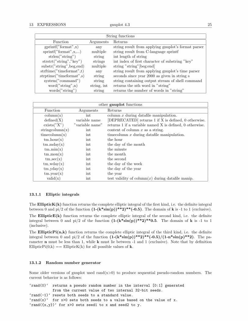
String functionsFunction Arguments Returns
gprintf(”format”,x) any string result from applying gnuplot’s format parsersprintf(”format”,x,...) multiple string result from C-language sprintf
strlen(”string”) string int length of stringstrstrt(”string”,”key”) strings int index of first character of substring ”key”substr(”string”,beg,end) multiple string ”string”[beg:end]strftime(”timeformat”,t) any string result from applying gnuplot’s time parserstrptime(”timeformat”,s) string seconds since year 2000 as given in string s
system(”command”) string string containing output stream of shell commandword(”string”,n) string, int returns the nth word in ”string”words(”string”) string returns the number of words in ”string”
other gnuplot functionsFunction Arguments Returnscolumn(x) int column x during datafile manipulation.defined(X) variable name [DEPRECATED] returns 1 if X is defined, 0 otherwise.exists(”X”) ”variable name” returns 1 if a variable named X is defined, 0 otherwise.
stringcolumn(x) int content of column x as a string.timecolumn(x) int timecolumn x during datafile manipulation.
tm hour(x) int the hourtm mday(x) int the day of the monthtm min(x) int the minutetm mon(x) int the monthtm sec(x) int the second
tm wday(x) int the day of the weektm yday(x) int the day of the yeartm year(x) int the year
valid(x) int test validity of column(x) during datafile manip.
13.1.1 Elliptic integrals
The EllipticK(k) function returns the complete elliptic integral of the first kind, i.e. the definite integralbetween 0 and pi/2 of the function (1-(k*sin(p))**2)**(-0.5). The domain of k is -1 to 1 (exclusive).
The EllipticE(k) function returns the complete elliptic integral of the second kind, i.e. the definiteintegral between 0 and pi/2 of the function (1-(k*sin(p))**2)**0.5. The domain of k is -1 to 1(inclusive).
The EllipticPi(n,k) function returns the complete elliptic integral of the third kind, i.e. the definiteintegral between 0 and pi/2 of the function (1-(k*sin(p))**2)**(-0.5)/(1-n*sin(p)**2). The pa-rameter n must be less than 1, while k must lie between -1 and 1 (exclusive). Note that by definitionEllipticPi(0,k) == EllipticK(k) for all possible values of k.
13.1.2 Random number generator
Some older versions of gnuplot used rand(x>0) to produce sequential pseudo-random numbers. Thecurrent behavior is as follows:
‘rand(0)‘ returns a pseudo random number in the interval [0:1] generatedfrom the current value of two internal 32-bit seeds.
‘rand(-1)‘ resets both seeds to a standard value.‘rand(x)‘ for x>0 sets both seeds to a value based on the value of x.‘rand({x,y})‘ for x>0 sets seed1 to x and seed2 to y.
26 gnuplot 4.3 13 EXPRESSIONS
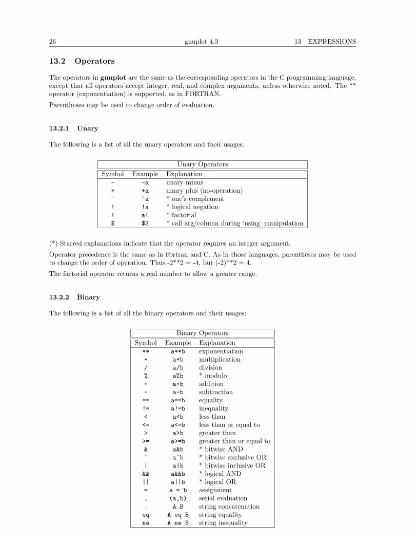
13.2 Operators
The operators in gnuplot are the same as the corresponding operators in the C programming language,except that all operators accept integer, real, and complex arguments, unless otherwise noted. The **operator (exponentiation) is supported, as in FORTRAN.
Parentheses may be used to change order of evaluation.
13.2.1 Unary
The following is a list of all the unary operators and their usages:
Unary OperatorsSymbol Example Explanation
- -a unary minus+ +a unary plus (no-operation)~ ~a * one’s complement! !a * logical negation! a! * factorial$ $3 * call arg/column during ‘using‘ manipulation
(*) Starred explanations indicate that the operator requires an integer argument.
Operator precedence is the same as in Fortran and C. As in those languages, parentheses may be usedto change the order of operation. Thus -2**2 = -4, but (-2)**2 = 4.
The factorial operator returns a real number to allow a greater range.
13.2.2 Binary
The following is a list of all the binary operators and their usages:
Binary OperatorsSymbol Example Explanation
** a**b exponentiation* a*b multiplication/ a/b division% a%b * modulo+ a+b addition- a-b subtraction== a==b equality!= a!=b inequality< a<b less than<= a<=b less than or equal to> a>b greater than>= a>=b greater than or equal to& a&b * bitwise AND^ a^b * bitwise exclusive OR| a|b * bitwise inclusive OR&& a&&b * logical AND|| a||b * logical OR= a = b assignment, (a,b) serial evaluation. A.B string concatenationeq A eq B string equalityne A ne B string inequality
13 EXPRESSIONS gnuplot 4.3 27
(*) Starred explanations indicate that the operator requires integer arguments. Capital letters A and Bindicate that the operator requires string arguments.
Logical AND (&&) and OR (||) short-circuit the way they do in C. That is, the second && operand isnot evaluated if the first is false; the second || operand is not evaluated if the first is true.
Serial evaluation occurs only in parentheses and is guaranteed to proceed in left to right order. Thevalue of the rightmost subexpression is returned.
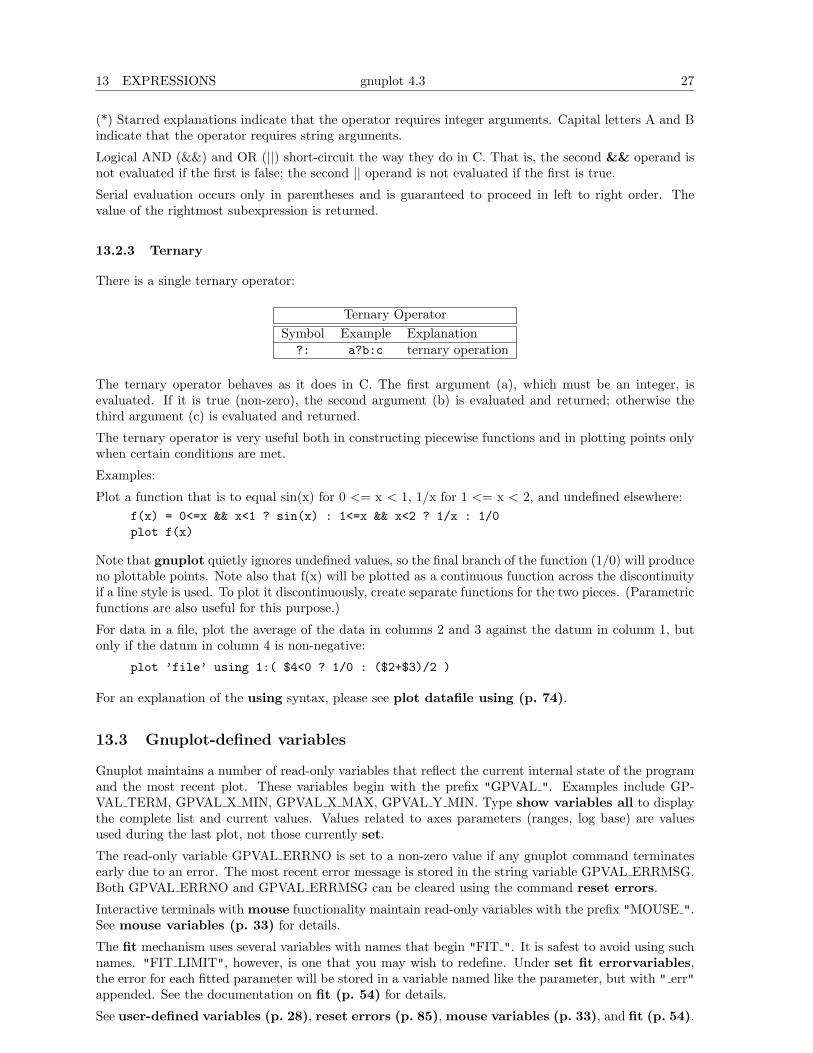
13.2.3 Ternary
There is a single ternary operator:
Ternary OperatorSymbol Example Explanation
?: a?b:c ternary operation
The ternary operator behaves as it does in C. The first argument (a), which must be an integer, isevaluated. If it is true (non-zero), the second argument (b) is evaluated and returned; otherwise thethird argument (c) is evaluated and returned.
The ternary operator is very useful both in constructing piecewise functions and in plotting points onlywhen certain conditions are met.
Examples:
Plot a function that is to equal sin(x) for 0 <= x < 1, 1/x for 1 <= x < 2, and undefined elsewhere:f(x) = 0<=x && x<1 ? sin(x) : 1<=x && x<2 ? 1/x : 1/0plot f(x)
Note that gnuplot quietly ignores undefined values, so the final branch of the function (1/0) will produceno plottable points. Note also that f(x) will be plotted as a continuous function across the discontinuityif a line style is used. To plot it discontinuously, create separate functions for the two pieces. (Parametricfunctions are also useful for this purpose.)
For data in a file, plot the average of the data in columns 2 and 3 against the datum in column 1, butonly if the datum in column 4 is non-negative:
plot ’file’ using 1:( $4<0 ? 1/0 : ($2+$3)/2 )
For an explanation of the using syntax, please see plot datafile using (p. 74).
13.3 Gnuplot-defined variables
Gnuplot maintains a number of read-only variables that reflect the current internal state of the programand the most recent plot. These variables begin with the prefix "GPVAL ". Examples include GP-VAL TERM, GPVAL X MIN, GPVAL X MAX, GPVAL Y MIN. Type show variables all to displaythe complete list and current values. Values related to axes parameters (ranges, log base) are valuesused during the last plot, not those currently set.
The read-only variable GPVAL ERRNO is set to a non-zero value if any gnuplot command terminatesearly due to an error. The most recent error message is stored in the string variable GPVAL ERRMSG.Both GPVAL ERRNO and GPVAL ERRMSG can be cleared using the command reset errors.
Interactive terminals with mouse functionality maintain read-only variables with the prefix "MOUSE ".See mouse variables (p. 33) for details.
The fit mechanism uses several variables with names that begin "FIT ". It is safest to avoid using suchnames. "FIT LIMIT", however, is one that you may wish to redefine. Under set fit errorvariables,the error for each fitted parameter will be stored in a variable named like the parameter, but with " err"appended. See the documentation on fit (p. 54) for details.
See user-defined variables (p. 28), reset errors (p. 85), mouse variables (p. 33), and fit (p. 54).
28 gnuplot 4.3 14 GLOSSARY
13.4 User-defined variables and functions
New user-defined variables and functions of one through five variables may be declared and used any-where, including on the plot command itself.
User-defined function syntax:<func-name>( <dummy1> {,<dummy2>} ... {,<dummy5>} ) = <expression>
where <expression> is defined in terms of <dummy1> through <dummy5>.
User-defined variable syntax:<variable-name> = <constant-expression>
Examples:w = 2q = floor(tan(pi/2 - 0.1))f(x) = sin(w*x)sinc(x) = sin(pi*x)/(pi*x)delta(t) = (t == 0)ramp(t) = (t > 0) ? t : 0min(a,b) = (a < b) ? a : bcomb(n,k) = n!/(k!*(n-k)!)len3d(x,y,z) = sqrt(x*x+y*y+z*z)plot f(x) = sin(x*a), a = 0.2, f(x), a = 0.4, f(x)
file = "mydata.inp"file(n) = sprintf("run_%d.dat",n)
The final two examples illustrate a user-defined string variable and a user-defined string function.
Note that the variables pi (3.14159...) and NaN (IEEE "Not a Number") are already defined. You canredefine these to something else if you really need to. The original values can be recovered by setting:
NaN = GPVAL_NaNpi = GPVAL_pi
Other variables may be defined under various gnuplot operations like mousing in interactive terminalsor fitting; see gnuplot-defined variables (p. 27) for details.
You can check for existence of a given variable V by the exists("V") expression. For examplea = 10if (exists("a")) print "a is defined"if (!exists("b")) print "b is not defined"
Valid names are the same as in most programming languages: they must begin with a letter, butsubsequent characters may be letters, digits, "$", or " ".
See show functions (p. 105), functions (p. 23), gnuplot-defined variables (p. 27), macros(p. 35).
14 Glossary
Throughout this document an attempt has been made to maintain consistency of nomenclature. Thiscannot be wholly successful because as gnuplot has evolved over time, certain command and keywordnames have been adopted that preclude such perfection. This section contains explanations of the waysome of these terms are used.
A "page" or "screen" or "canvas" is the entire area addressable by gnuplot. On a desktop it is a fullwindow; on a plotter, it is a single sheet of paper; in svga mode it is the full monitor screen.
A screen may contain one or more "plots". A plot is defined by an abscissa and an ordinate, althoughthese need not actually appear on it, as well as the margins and any text written therein.
15 LINETYPE, COLORS, AND STYLES gnuplot 4.3 29
A plot contains one "graph". A graph is defined by an abscissa and an ordinate, although these neednot actually appear on it.
A graph may contain one or more "lines". A line is a single function or data set. "Line" is also a plottingstyle. The word will also be used in sense "a line of text". Presumably the context will remove anyambiguity.
The lines on a graph may have individual names. These may be listed together with a sample of theplotting style used to represent them in the "key", sometimes also called the "legend".
The word "title" occurs with multiple meanings in gnuplot. In this document, it will always be precededby the adjective "plot", "line", or "key" to differentiate among them. A 2D graph may have up to fourlabelled axes. The names of the four axes are "x" for the axis along the bottom border of the plot,"y" for the axis along the left border, "x2" for the top border, and "y2" for the right border. See axes(p. 64).
A 3D graph may have up to three labelled axes – "x", "y" and "z". It is not possible to say where onthe graph any particular axis will fall because you can change the direction from which the graph is seenwith set view.
When discussing data files, the term "record" will be resurrected and used to denote a single line of textin the file, that is, the characters between newline or end-of-record characters. A "point" is the datumextracted from a single record. A "datablock" is a set of points from consecutive records, delimited byblank records. A line, when referred to in the context of a data file, is a subset of a datablock.
15 Linetype, colors, and styles
Each gnuplot terminal type provides a set of distinct "linetypes". These may differ in color, in thickness,in dot/dash pattern, or in some combination of color and dot/dash. The default linetypes for a particularterminal can be previewed by issuing the test command after setting the terminal type. The pre-defined colors and dot/dash patterns are not guaranteed to be consistent for all terminal types, butall terminals use the special linetype -1 to mean a solid line in the primary foreground color (normallyblack). By default, successive functions or datafiles plotted by a single command will be assignedsuccessive linetypes. You can override this default by specifying a particular linetype for any function,datafile, or plot element.
Examples:plot "foo", "bar" # plot two files using linetypes 1, 2plot sin(x) linetype 4 # terminal-specific linetype color 4plot sin(x) lt -1 # black
For many terminal types it is also possible to assign user-defined colors using explicit rgb (red, green,blue) values, named colors, or color values that refer to the current PM3D palette.
Examples:plot sin(x) lt rgb "violet" # one of gnuplot’s named colorsplot sin(x) lt rgb "#FF00FF" # explicit RGB triple in hexadecimalplot sin(x) lt palette cb -45 # whatever color corresponds to -45
# in the current cbrange of the paletteplot sin(x) lt palette frac 0.3 # fractional value along the palette
See show colornames (p. 95), set palette (p. 126), cbrange (p. 153).
For terminals that support dot/dash patterns, each default linetype has both a dot-dash pattern and adefault color. However, you can override the default color by using the keyword linecolor, abbreviatedlc. For example, the postscript terminal provides a dashed blue line as linetype 3. The plot commandsbelow use this same dash pattern for three plots, one in blue (the default), another in red (the defaultfor linetype 1), and a third in gold.
Example:set term postscript dashed colorplot ’foo’ lt 3, ’baz’ lt 3 linecolor 1, ’bar’ lt 3 lc rgb ’gold’
30 gnuplot 4.3 15 LINETYPE, COLORS, AND STYLES
Lines can have additional properties such as linewidth. You can associate these various properties, aswell as equivalent properties for point symbols, into user-defined "line styles" using the command setstyle line. Once you have defined a linestyle, you can use it in a plot command to control the appearanceof one or more plot elements.
Examples:# define a new line style with terminal-independent color cyan,# linewidth 3, and associated point type 6 (a circle with a dot in it).set style line 5 lt rgb "cyan" lw 3 pt 6plot sin(x) with linespoints ls 5 # user-defined line style 5
See linestyle (p. 136), set style line (p. 136).
15.1 Colorspec
Many commands allow you to specify a linetype with an explicit color. Terminal-independent colorchoice is only possible for terminals that support RGB color or pm3d palettes.
Syntax:... {linecolor | lc} <colorspec>... {textcolor | tc} <colorspec>
where <colorspec> has one of the following forms:rgbcolor "colorname"rgbcolor "#RRGGBB"rgbcolor variable # color is read from input filepalette frac <val> # <val> runs from 0 to 1palette cb <value> # <val> lies within cbrangepalette zvariable # color index is read from input file
"colorname" refers to one of the color names built in to gnuplot. For a list of the available names, seeshow colornames (p. 95).
"#RRGGBB" is a hexadecimal constant preceded by the "#" symbol. The RRGGBB represents thered, green, and blue components of the color, each on a scale from 0 - 255. For example, magenta = full-scale red + full-scale blue would be represented by #FF00FF, which is the hexadecimal representationof (255 << 16) + (0 << 8) + (255).
The color palette is a linear gradient of colors that smoothly maps a single numerical value onto aparticular color. Two such mappings are always in effect. palette frac maps a fractional value between0 and 1 onto the full range of the color palette. palette cb maps the range of the color axis onto thesame palette. See set cbrange (p. 153). See also set colorbox (p. 94). You can use either of theseto select a constant color from the current palette.
"palette z" maps the z value of each plot segment or plot element into the cbrange mapping of thepalette. This allows smoothly-varying color along a 3d line or surface. It also allows coloring 2D plotsby palette values read from an extra column of data (not all 2D plot styles allow an extra column).
15.1.1 Rgbcolor variable
Most plot commands assign a single color (linetype) to each element of the plot. If there are multipleplots on a single graph, the default color (linetype) is incremented sequentially. You can instead assigna separate color for each data point, line segment, or label based on additional information in the inputdata file. This is indicated by the colorspec keyword variable.
lc rgbcolor variable tells the program to use a 24-bit RGB color from a separate column in the data file.This requires a corresponding additional column in the using specifier. The extra column is interpretedas a 24-bit packed RGB triple. These are most easily specified as hexidecimal values (see rgbcolor(p. 30)). Text colors are similarly set using tc rgbcolor variable.
Example:

16 MOUSE INPUT gnuplot 4.3 31
# Place colored points in 3D at the x,y,z coordinates corresponding to# their red, green, and blue componentsrgb(r,g,b) = 65536 * int(r) + 256 * int(g) + int(b)splot "data" using 1:2:3:(rgb($1,$2,$3)) with points lc rgb variable
15.1.2 Linecolor variable
Most plot commands assign a single color (linetype) to each element of the plot. If there are multipleplots on a single graph, the default color (linetype) is incremented sequentially. You can instead assigna separate color for each data point, line segment, or label based on additional information in the inputdata file. This is indicated by the colorspec keyword variable.
lc variable tells the program to use the value read from one column of the input data as a linestyleindex, and use the color belonging to that linestyle. This requires a corresponding additional column inthe using specifier. Text colors can be set similarly using tc variable.
A single data file may contain multiple sets of data, separated by two blank lines. Each of these separatesets is assigned an index value (see index (p. 71)) that can be retrieved via the using specifier column(-2). See pseudocolumns (p. 76). All data in the file is drawn with the same color/linestyle/pointtypeproperties by default. The command lc variable can be used to assign different colors to each data setin the file by using the index value from pseudocolumn -2.
Examples:# Use the third column of data to assign colors to individual pointsplot ’data’ using 1:2:3 with points lc variable
# Use the data set index to choose a linestyle colorplot ’data’ using 1:2:(column(-2)) with lines lc variable
16 Mouse input
The x11, pm, windows, ggi, and wxt terminals allow interaction with the current plot using themouse. They also support the definition of hotkeys to activate pre-defined functions by hitting a singlekey while the mouse focus is in the active plot window. It is even possible to combine mouse input withbatch command scripts, by invoking the command pause mouse and then using the mouse variablesreturned by mouse clicking as parameters for subsequent scripted actions. See bind (p. 31) and mousevariables (p. 33). See also the command set mouse (p. 115).
16.1 Bind
Syntax:bind {allwindows} [<key-sequence>] ["<gnuplot commands>"]bind <key-sequence> ""reset bind
The bind allows defining or redefining a hotkey, i.e. a sequence of gnuplot commands which will beexecuted when a certain key or key sequence is pressed while the driver’s window has the input focus.Note that bind is only available if gnuplot was compiled with mouse support and it is used by all mouse-capable terminals. A user-specified binding supersedes any builtin bindings, except that <space> and’q’ cannot normally be rebound. For an exception, see bind space (p. 33).
Mouse buttons cannot be rebound.
You get the list of all hotkeys by typing show bind or bind or by typing the hotkey ’h’ in the graphwindow.
Key bindings are restored to their default state by reset bind.

32 gnuplot 4.3 16 MOUSE INPUT
Note that multikey-bindings with modifiers must be given in quotes.
Normally hotkeys are only recognized when the currently active plot window has focus. bind allwin-dows <key> ... (short form: bind all <key> ...) causes the binding for <key> to apply to allgnuplot plot windows, active or not. In this case gnuplot variable MOUSE KEY WINDOW is set to theID of the originating window, and may be used by the bound command.
Examples:
- set bindings:
bind a "replot"bind "ctrl-a" "plot x*x"bind "ctrl-alt-a" ’print "great"’bind Home "set view 60,30; replot"bind all Home ’print "This is window ",MOUSE_KEY_WINDOW’
- show bindings:
bind "ctrl-a" # shows the binding for ctrl-abind # shows all bindingsshow bind # show all bindings
- remove bindings:
bind "ctrl-alt-a" "" # removes binding for ctrl-alt-a(note that builtins cannot be removed)
reset bind # installs default (builtin) bindingsbind! # deprecated form of "reset bind"
- bind a key to toggle something:
v=0bind "ctrl-r" "v=v+1;if(v%2)set term x11 noraise; else set term x11 raise"
Modifiers (ctrl / alt) are case insensitive, keys not:
ctrl-alt-a == CtRl-alT-actrl-alt-a != ctrl-alt-A
List of modifiers (alt == meta):
ctrl, alt
List of supported special keys:
"BackSpace", "Tab", "Linefeed", "Clear", "Return", "Pause", "Scroll_Lock","Sys_Req", "Escape", "Delete", "Home", "Left", "Up", "Right", "Down","PageUp", "PageDown", "End", "Begin",
"KP_Space", "KP_Tab", "KP_Enter", "KP_F1", "KP_F2", "KP_F3", "KP_F4","KP_Home", "KP_Left", "KP_Up", "KP_Right", "KP_Down", "KP_PageUp","KP_PageDown", "KP_End", "KP_Begin", "KP_Insert", "KP_Delete", "KP_Equal","KP_Multiply", "KP_Add", "KP_Separator", "KP_Subtract", "KP_Decimal","KP_Divide",
"KP_1" - "KP_9", "F1" - "F12"
The following are window events rather than actual keys
"Close"
See also help for mouse (p. 115) and if (p. 61).
17 PLOTTING gnuplot 4.3 33
16.1.1 Bind space
If gnuplot was built with configuration option –enable-raise-console, then typing <space> in the plotwindow raises gnuplot’s command window. This hotkey can be changed to ctrl-space by starting gnuplotas ’gnuplot -ctrlq’, or by setting the XResource ’gnuplot*ctrlq’. See x11 command-line-options(p. 207).
16.2 Mouse variables
When mousing is active, clicking in the active window will set several user variables that can be accessedfrom the gnuplot command line. The coordinates of the mouse at the time of the click are storedin MOUSE X MOUSE Y MOUSE X2 and MOUSE Y2. The mouse button clicked, and any meta-keysactive at that time, are stored in MOUSE BUTTON MOUSE SHIFT MOUSE ALT and MOUSE CTRL.These variables are set to undefined at the start of every plot, and only become defined in the event of amouse click in the active plot window. To determine from a script if the mouse has been clicked in theactive plot window, it is sufficient to test for any one of these variables being defined.
plot ’something’pause mouseif (defined(MOUSE_BUTTON)) call ’something_else’; \else print "No mouse click."
It is also possible to track keystrokes in the plot window using the mousing code.
plot ’something’pause mouse keypressprint "Keystroke ", MOUSE_KEY, " at ", MOUSE_X, " ", MOUSE_Y
When pause mouse keypress is terminated by a keypress, then MOUSE KEY will contain the asciicharacter value of the key that was pressed. MOUSE CHAR will contain the character itself as a stringvariable. If the pause command is terminated abnormally (e.g. by ctrl-C or by externally closing theplot window) then MOUSE KEY will equal -1.
Note that after a zoom by mouse, you can read the new ranges as GPVAL X MIN, GPVAL X MAX,GPVAL Y MIN, and GPVAL Y MAX, see gnuplot-defined variables (p. 27).
17 Plotting
There are three gnuplot commands which actually create a plot: plot, splot and replot. plot gen-erates 2D plots, splot generates 3-d plots (actually 2D projections, of course), and replot appends itsarguments to the previous plot or splot and executes the modified command.
Much of the general information about plotting can be found in the discussion of plot; informationspecific to 3D can be found in the splot section.
plot operates in either rectangular or polar coordinates – see set polar (p. 131) for details of thelatter. splot operates only in rectangular coordinates, but the set mapping command allows for a fewother coordinate systems to be treated. In addition, the using option allows both plot and splot totreat almost any coordinate system you’d care to define.
plot also lets you use each of the four borders – x (bottom), x2 (top), y (left) and y2 (right) – as anindependent axis. The axes option lets you choose which pair of axes a given function or data set isplotted against. A full complement of set commands exists to give you complete control over the scalesand labelling of each axis. Some commands have the name of an axis built into their names, such as setxlabel. Other commands have one or more axis names as options, such as set logscale xy. Commandsand options controlling the z axis have no effect on 2D graphs.
splot can plot surfaces and contours in addition to points and/or lines. In addition to splot, see setisosamples (p. 108) for information about defining the grid for a 3D function; splot datafile (p. 154)
34 gnuplot 4.319 STRING CONSTANTS AND STRING VARIABLES
for information about the requisite file structure for 3D data values; and set contour (p. 95) and setcntrparam (p. 93) for information about contours.
In splot, control over the scales and labels of the axes are the same as with plot, except that commandsand options controlling the x2 and y2 axes have no effect whereas of course those controlling the z axisdo take effect.
18 Start-up
When gnuplot is run, it looks for an initialization file to load. This file is called .gnuplot on Unixand AmigaOS systems, and GNUPLOT.INI on other systems. If this file is not found in the currentdirectory, the program will look for it in the HOME directory (under AmigaOS, MS-DOS, Windows andOS/2, the environment variable GNUPLOT should contain the name of this directory; on WindowsNT, it will use USERPROFILE if GNUPLOT isn’t defined). Note: if NOCWDRC is defined duringthe installation, gnuplot will not read from the current directory.
If the initialization file is found, gnuplot executes the commands in it. These may be any legal gnuplotcommands, but typically they are limited to setting the terminal and defining frequently-used functionsor variables.
19 String constants and string variables
In addition to string constants, most gnuplot commands also accept a string variable, a string expression,or a function that returns a string. For example, the following four methods of creating a plot all resultin the same plot title:
four = "4"graph4 = "Title for plot #4"graph(n) = sprintf("Title for plot #%d",n)
plot ’data.4’ title "Title for plot #4"plot ’data.4’ title graph4plot ’data.4’ title "Title for plot #".fourplot ’data.4’ title graph(4)
Since integers are promoted to strings when operated on by the string concatenation operator, thefollowing method also works:
N = 4plot ’data.’.N title "Title for plot #".N
In general, elements on the command line will only be evaluated as possible string variables if they arenot otherwise recognizable as part of the normal gnuplot syntax. So the following sequence of commandsis legal, although probably should be avoided so as not to cause confusion:
plot = "my_datafile.dat"title = "My Title"plot plot title title
There are three binary operators that require string operands: the string concatenation operator ".",the string equality operator "eq" and the string inequality operator "ne". The following example willprint TRUE.
if ("A"."B" eq "AB") print "TRUE"
See also the two string formatting functions gprintf (p. 103) and sprintf (p. 25).
Substrings can be specified by appending a range specifier to any string, string variable, or string-valuedfunction. The range specifier has the form [begin:end], where begin is the index of the first character ofthe substring and end is the index of the last character of the substring. The first character has index1. The begin or end fields may be empty, or contain ’*’, to indicate the true start or end of the originalstring. E.g. str[:] and str[*:*] both describe the full string str.
20 SUBSTITUTION AND COMMAND LINE MACROSgnuplot 4.3 35
20 Substitution and Command line macros
When a command line to gnuplot is first read, i.e. before it is interpreted or executed, two forms oflexical substitution are performed. These are triggered by the presence of text in backquotes (asciicharacter 96) or preceded by @ (ascii character 64).
20.1 Substitution of system commands in backquotes
Command-line substitution is specified by a system command enclosed in backquotes. This commandis spawned and the output it produces replaces the backquoted text on the command line. Someimplementations also support pipes; see plot datafile special-filenames (p. 73).
Command-line substitution can be used anywhere on the gnuplot command line, except inside stringsdelimited by single quotes.
Example:
This will run the program leastsq and replace leastsq (including backquotes) on the command linewith its output:
f(x) = ‘leastsq‘
or, in VMSf(x) = ‘run leastsq‘
These will generate labels with the current time and userid:set label "generated on ‘date +%Y-%m-%d‘ by ‘whoami‘" at 1,1set timestamp "generated on %Y-%m-%d by ‘whoami‘"
20.2 Substitution of string variables as macros
Substitution of command line macros is disabled by default, but may be enabled using the set macroscommand. If macro substitution is enabled, the character @ is used to trigger substitution of the currentvalue of a string variable into the command line. The text in the string variable may contain anynumber of lexical elements. This allows string variables to be used as command line macros. Only stringconstants may be expanded using this mechanism, not string-valued expressions. For example:
set macrosstyle1 = "lines lt 4 lw 2"style2 = "points lt 3 pt 5 ps 2"range1 = "using 1:3"range2 = "using 1:5"plot "foo" @range1 with @style1, "bar" @range2 with @style2
The line containing @ symbols is expanded on input, so that by the time it is executed the effect isidentical to having typed in full
plot "foo" using 1:3 with lines lt 4 lw 2, \"bar" using 1:5 with points lt 3 pt 5 ps 2
The function exists() may be useful in connection with macro evaluation. The following example checksthat C can safely be expanded as the name of a user-defined variable:
C = "pi"if (exists(C)) print C," = ", @C
Macro expansion does not occur inside either single or double quotes. However macro expansion doesoccur inside backquotes.
For execution of complete commands the evaluate command may also be handy.
36 gnuplot 4.3 21 SYNTAX
20.3 String variables, macros, and command line substitution
The interaction of string variables, backquotes and macro substitution is somewhat complicated. Back-quotes do not block macro substitution, so
filename = "mydata.inp"lines = ‘ wc --lines @filename | sed "s/ .*//" ‘
results in the number of lines in mydata.inp being stored in the integer variable lines. And double quotesdo not block backquote substitution, so
mycomputer = "‘uname -n‘"
results in the string returned by the system command uname -n being stored in the string variablemycomputer.
However, macro substitution is not performed inside double quotes, so you cannot define a systemcommand as a macro and then use both macro and backquote substitution at the same time.
machine_id = "uname -n"mycomputer = "‘@machine_id‘" # doesn’t work!!
This fails because the double quotes prevent @machine id from being interpreted as a macro. To storea system command as a macro and execute it later you must instead include the backquotes as part ofthe macro itself. This is accomplished by defining the macro as shown below. Notice that the sprintfformat nests all three types of quotes.
machine_id = sprintf(’"‘uname -n‘"’)mycomputer = @machine_id
21 Syntax
Version 4 of gnuplot is much less sensitive than earlier versions to the order of keywords and suboptions.However, if you get error messages from specifying options that you think should work, please tryrearranging them into the exact order listed by the documentation.
Options and any accompanying parameters are separated by spaces whereas lists and coordinates areseparated by commas. Ranges are separated by colons and enclosed in brackets [], text and file namesare enclosed in quotes, and a few miscellaneous things are enclosed in parentheses. Braces {} are usedfor a few special purposes.
Commas are used to separate coordinates on the set commands arrow, key, and label; the list ofvariables being fitted (the list after the via keyword on the fit command); lists of discrete contours orthe loop parameters which specify them on the set cntrparam command; the arguments of the setcommands dgrid3d, dummy, isosamples, offsets, origin, samples, size, time, and view; lists oftics or the loop parameters which specify them; the offsets for titles and axis labels; parametric functionsto be used to calculate the x, y, and z coordinates on the plot, replot and splot commands; and thecomplete sets of keywords specifying individual plots (data sets or functions) on the plot, replot andsplot commands.
Parentheses are used to delimit sets of explicit tics (as opposed to loop parameters) and to indicatecomputations in the using filter of the fit, plot, replot and splot commands.
(Parentheses and commas are also used as usual in function notation.)
Square brackets are used to delimit ranges given in set, plot or splot commands.
Colons are used to separate extrema in range specifications (whether they are given on set, plot orsplot commands) and to separate entries in the using filter of the plot, replot, splot and fit commands.
Semicolons are used to separate commands given on a single command line.
Braces are used in text to be specially processed by some terminals, like postscript. They are also usedto denote complex numbers: {3,2} = 3 + 2i.
22 TIME/DATE DATA gnuplot 4.3 37
At present you should not embed \n inside {} when using the PostScript terminal in enhanced textmode.
The EEPIC, Imagen, Uniplex, LaTeX, and TPIC drivers allow a newline to be specified by \\ in asingle-quoted string or \\\\ in a double-quoted string.
21.1 Quote Marks
Gnuplot uses three forms of quote marks for delimiting text strings, double-quote (ascii 34), single-quote(ascii 39), and backquote (ascii 96).
Filenames may be entered with either single- or double-quotes. In this manual the command examplesgenerally single-quote filenames and double-quote other string tokens for clarity.
String constants and text strings used for labels, titles, or other plot elements may be enclosed in eithersingle quotes or double quotes. Further processing of the quoted text depends on the choice of quotemarks.
Backslash processing of special characters like \n (newline) and \345 (octal character code) is performedfor double-quoted strings. In single-quoted strings, backslashes are just ordinary characters. To get asingle-quote (ascii 39) in a single-quoted string, it has to be doubled. Thus the strings "d\" s’ b\\" and’d" s’ ’ b\’ are completely equivalent.
Text justification is the same for each line of a multi-line string. Thus the center-justified string"This is the first line of text.\nThis is the second line."
will produceThis is the first line of text.
This is the second line.
but’This is the first line of text.\nThis is the second line.’
will produceThis is the first line of text.\nThis is the second line.
Enhanced text processing is performed for both double-quoted text and single-quoted text, but only byterminals supporting this mode. See enhanced text (p. 21).
Back-quotes are used to enclose system commands for substitution into the command line. See substi-tution (p. 35).
22 Time/Date data
gnuplot supports the use of time and/or date information as input data. This feature is activated bythe commands set xdata time, set ydata time, etc.
Internally all times and dates are converted to the number of seconds from the year 2000. The commandset timefmt defines the format for all inputs: data files, ranges, tics, label positions — in short, anythingthat accepts a data value must receive it in this format. Since only one input format can be in forceat a given time, all time/date quantities being input at the same time must be presented in the sameformat. Thus if both x and y data in a file are time/date, they must be in the same format.
The conversion to and from seconds assumes Universal Time (which is the same as Greenwich StandardTime). There is no provision for changing the time zone or for daylight savings. If all your data refer tothe same time zone (and are all either daylight or standard) you don’t need to worry about these things.But if the absolute time is crucial for your application, you’ll need to convert to UT yourself.
Commands like show xrange will re-interpret the integer according to timefmt. If you changetimefmt, and then show the quantity again, it will be displayed in the new timefmt. For that matter,if you give the deactivation command (like set xdata), the quantity will be shown in its numerical form.
38 gnuplot 4.3 23 BOXERRORBARS
The commands set format or set tics format define the format that will be used for tic labels, whetheror not the specified axis is time/date.
If time/date information is to be plotted from a file, the using option must be used on the plot orsplot command. These commands simply use white space to separate columns, but white space maybe embedded within the time/date string. If you use tabs as a separator, some trial-and-error may benecessary to discover how your system treats them.
The following example demonstrates time/date plotting.
Suppose the file "data" contains records like
03/21/95 10:00 6.02e23
This file can be plotted by
set xdata timeset timefmt "%m/%d/%y"set xrange ["03/21/95":"03/22/95"]set format x "%m/%d"set timefmt "%m/%d/%y %H:%M"plot "data" using 1:3
which will produce xtic labels that look like "03/21".
See the descriptions of each command for more details.
Part II
Plotting styles
There are many plotting styles available in gnuplot. They are listed alphabetically below. The commandsset style data and set style function change the default plotting style for subsequent plot and splotcommands.
You also have the option to specify the plot style explicitly as part of the plot or splot command. Ifyou want to mix plot styles within a single plot, you must specify the plot style for each component.
Example:
plot ’data’ with boxes, sin(x) with lines
Each plot style has its own expected set of data entries in a data file. For example by default the linesstyle expects either a single column of y values (with implicit x ordering) or a pair of columns with xin the first and y in the second. For more information on how to fine-tune how columns in a file areinterpreted as plot data, see using (p. 74).
23 Boxerrorbars
The boxerrorbars style is only relevant to 2D data plotting. It is a combination of the boxes andyerrorbars styles. It uses 3, 4, or 5 columns of data:
3 columns: x y ydelta4 columns: x y ydelta xdelta # boxwidth != -24 columns: x y ylow yhigh # boxwidth == -25 columns: x y ylow yhigh xdelta
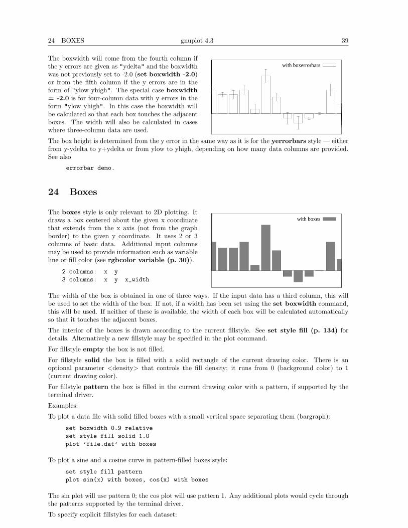
24 BOXES gnuplot 4.3 39
with boxerrorbarsThe boxwidth will come from the fourth column ifthe y errors are given as "ydelta" and the boxwidthwas not previously set to -2.0 (set boxwidth -2.0)or from the fifth column if the y errors are in theform of "ylow yhigh". The special case boxwidth= -2.0 is for four-column data with y errors in theform "ylow yhigh". In this case the boxwidth willbe calculated so that each box touches the adjacentboxes. The width will also be calculated in caseswhere three-column data are used.
The box height is determined from the y error in the same way as it is for the yerrorbars style — eitherfrom y-ydelta to y+ydelta or from ylow to yhigh, depending on how many data columns are provided.See also
errorbar demo.
24 Boxes
with boxesThe boxes style is only relevant to 2D plotting. Itdraws a box centered about the given x coordinatethat extends from the x axis (not from the graphborder) to the given y coordinate. It uses 2 or 3columns of basic data. Additional input columnsmay be used to provide information such as variableline or fill color (see rgbcolor variable (p. 30)).
2 columns: x y3 columns: x y x_width
The width of the box is obtained in one of three ways. If the input data has a third column, this willbe used to set the width of the box. If not, if a width has been set using the set boxwidth command,this will be used. If neither of these is available, the width of each box will be calculated automaticallyso that it touches the adjacent boxes.
The interior of the boxes is drawn according to the current fillstyle. See set style fill (p. 134) fordetails. Alternatively a new fillstyle may be specified in the plot command.
For fillstyle empty the box is not filled.
For fillstyle solid the box is filled with a solid rectangle of the current drawing color. There is anoptional parameter <density> that controls the fill density; it runs from 0 (background color) to 1(current drawing color).
For fillstyle pattern the box is filled in the current drawing color with a pattern, if supported by theterminal driver.
Examples:
To plot a data file with solid filled boxes with a small vertical space separating them (bargraph):
set boxwidth 0.9 relativeset style fill solid 1.0plot ’file.dat’ with boxes
To plot a sine and a cosine curve in pattern-filled boxes style:
set style fill patternplot sin(x) with boxes, cos(x) with boxes
The sin plot will use pattern 0; the cos plot will use pattern 1. Any additional plots would cycle throughthe patterns supported by the terminal driver.
To specify explicit fillstyles for each dataset:
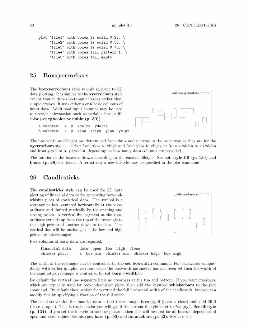
40 gnuplot 4.3 26 CANDLESTICKS
plot ’file1’ with boxes fs solid 0.25, \’file2’ with boxes fs solid 0.50, \’file3’ with boxes fs solid 0.75, \’file4’ with boxes fill pattern 1, \’file5’ with boxes fill empty
25 Boxxyerrorbars
with boxxyerrorbarsThe boxxyerrorbars style is only relevant to 2Ddata plotting. It is similar to the xyerrorbars styleexcept that it draws rectangular areas rather thansimple crosses. It uses either 4 or 6 basic columns ofinput data. Additional input columns may be usedto provide information such as variable line or fillcolor (see rgbcolor variable (p. 30)).
4 columns: x y xdelta ydelta6 columns: x y xlow xhigh ylow yhigh
The box width and height are determined from the x and y errors in the same way as they are for thexyerrorbars style — either from xlow to xhigh and from ylow to yhigh, or from x-xdelta to x+xdeltaand from y-ydelta to y+ydelta, depending on how many data columns are provided.
The interior of the boxes is drawn according to the current fillstyle. See set style fill (p. 134) andboxes (p. 39) for details. Alternatively a new fillstyle may be specified in the plot command.
26 Candlesticks
with candlesticksThe candlesticks style can be used for 2D dataplotting of financial data or for generating box-and-whisker plots of statistical data. The symbol is arectangular box, centered horizontally at the x co-ordinate and limited vertically by the opening andclosing prices. A vertical line segment at the x co-ordinate extends up from the top of the rectangle tothe high price and another down to the low. Thevertical line will be unchanged if the low and highprices are interchanged.
Five columns of basic data are required:
financial data: date open low high closewhisker plot: x box_min whisker_min whisker_high box_high
The width of the rectangle can be controlled by the set boxwidth command. For backwards compat-ibility with earlier gnuplot versions, when the boxwidth parameter has not been set then the width ofthe candlestick rectangle is controlled by set bars <width>.
By default the vertical line segments have no crossbars at the top and bottom. If you want crossbars,which are typically used for box-and-whisker plots, then add the keyword whiskerbars to the plotcommand. By default these whiskerbars extend the full horizontal width of the candlestick, but you canmodify this by specifying a fraction of the full width.
The usual convention for financial data is that the rectangle is empty if (open < close) and solid fill if(close < open). This is the behavior you will get if the current fillstyle is set to "empty". See fillstyle(p. 134). If you set the fillstyle to solid or pattern, then this will be used for all boxes independent ofopen and close values. See also set bars (p. 90) and financebars (p. 42). See also the
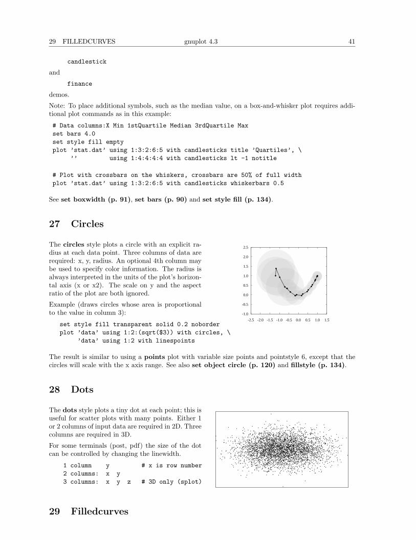
29 FILLEDCURVES gnuplot 4.3 41
candlestick
and
finance
demos.
Note: To place additional symbols, such as the median value, on a box-and-whisker plot requires addi-tional plot commands as in this example:
# Data columns:X Min 1stQuartile Median 3rdQuartile Maxset bars 4.0set style fill emptyplot ’stat.dat’ using 1:3:2:6:5 with candlesticks title ’Quartiles’, \
’’ using 1:4:4:4:4 with candlesticks lt -1 notitle
# Plot with crossbars on the whiskers, crossbars are 50% of full widthplot ’stat.dat’ using 1:3:2:6:5 with candlesticks whiskerbars 0.5
See set boxwidth (p. 91), set bars (p. 90) and set style fill (p. 134).
27 Circles
-1.0
-0.5
0.0
0.5
1.0
1.5
2.0
2.5
-2.5 -2.0 -1.5 -1.0 -0.5 0.0 0.5 1.0 1.5
The circles style plots a circle with an explicit ra-dius at each data point. Three columns of data arerequired: x, y, radius. An optional 4th column maybe used to specify color information. The radius isalways interpreted in the units of the plot’s horizon-tal axis (x or x2). The scale on y and the aspectratio of the plot are both ignored.
Example (draws circles whose area is proportionalto the value in column 3):
set style fill transparent solid 0.2 noborderplot ’data’ using 1:2:(sqrt($3)) with circles, \
’data’ using 1:2 with linespoints
The result is similar to using a points plot with variable size points and pointstyle 6, except that thecircles will scale with the x axis range. See also set object circle (p. 120) and fillstyle (p. 134).
28 Dots
The dots style plots a tiny dot at each point; this isuseful for scatter plots with many points. Either 1or 2 columns of input data are required in 2D. Threecolumns are required in 3D.
For some terminals (post, pdf) the size of the dotcan be controlled by changing the linewidth.
1 column y # x is row number2 columns: x y3 columns: x y z # 3D only (splot)
29 Filledcurves
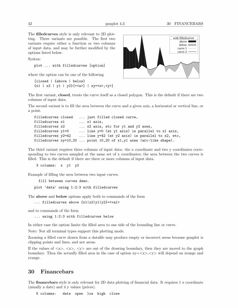
42 gnuplot 4.3 30 FINANCEBARS
with filledcurvesabovebelow
curve 1curve 2
The filledcurves style is only relevant to 2D plot-ting. Three variants are possible. The first twovariants require either a function or two columnsof input data, and may be further modified by theoptions listed below.
Syntax:
plot ... with filledcurves [option]
where the option can be one of the following
[closed | {above | below}{x1 | x2 | y1 | y2}[=<a>] | xy=<x>,<y>]
The first variant, closed, treats the curve itself as a closed polygon. This is the default if there are twocolumns of input data.
The second variant is to fill the area between the curve and a given axis, a horizontal or vertical line, ora point.
filledcurves closed ... just filled closed curve,filledcurves x1 ... x1 axis,filledcurves x2 ... x2 axis, etc for y1 and y2 axes,filledcurves y1=0 ... line y=0 (at y1 axis) ie parallel to x1 axis,filledcurves y2=42 ... line y=42 (at y2 axis) ie parallel to x2, etc,filledcurves xy=10,20 ... point 10,20 of x1,y1 axes (arc-like shape).
The third variant requires three columns of input data: the x coordinate and two y coordinates corre-sponding to two curves sampled at the same set of x coordinates; the area between the two curves isfilled. This is the default if there are three or more columns of input data.
3 columns: x y1 y2
Example of filling the area between two input curves.
fill between curves demo.
plot ’data’ using 1:2:3 with filledcurves
The above and below options apply both to commands of the form... filledcurves above {x1|x2|y1|y2}=<val>
and to commands of the form... using 1:2:3 with filledcurves below
In either case the option limits the filled area to one side of the bounding line or curve.
Note: Not all terminal types support this plotting mode.
Zooming a filled curve drawn from a datafile may produce empty or incorrect areas because gnuplot isclipping points and lines, and not areas.
If the values of <a>, <x>, <y> are out of the drawing boundary, then they are moved to the graphboundary. Then the actually filled area in the case of option xy=<x>,<y> will depend on xrange andyrange.
30 Financebars
The financebars style is only relevant for 2D data plotting of financial data. It requires 1 x coordinate(usually a date) and 4 y values (prices).
5 columns: date open low high close

33 HISTOGRAMS gnuplot 4.3 43
with financebarsThe symbol is a vertical line segment, located hori-zontally at the x coordinate and limited vertically bythe high and low prices. A horizontal tic on the leftmarks the opening price and one on the right marksthe closing price. The length of these tics may bechanged by set bars. The symbol will be unchangedif the high and low prices are interchanged. See setbars (p. 90) and candlesticks (p. 40), and alsothe
finance demo.
31 Fsteps
with fstepsThe fsteps style is only relevant to 2D plotting. Itconnects consecutive points with two line segments:the first from (x1,y1) to (x1,y2) and the second from(x1,y2) to (x2,y2). The input column requires arethe same as for plot styles lines and points. Thedifference between fsteps and steps is that fstepstraces first the change in y and then the change inx. steps traces first the change in x and then thechange in y.
See also
steps demo.
32 Histeps
with histepsThe histeps style is only relevant to 2D plotting.It is intended for plotting histograms. Y-valuesare assumed to be centered at the x-values; thepoint at x1 is represented as a horizontal line from((x0+x1)/2,y1) to ((x1+x2)/2,y1). The lines repre-senting the end points are extended so that the stepis centered on at x. Adjacent points are connectedby a vertical line at their average x, that is, from((x1+x2)/2,y1) to ((x1+x2)/2,y2). The input col-umn requires are the same as for plot styles linesand points.
If autoscale is in effect, it selects the xrange from the data rather than the steps, so the end points willappear only half as wide as the others. See also
steps demo.
histeps is only a plotting style; gnuplot does not have the ability to create bins and determine theirpopulation from some data set.
33 Histograms
The histograms style is only relevant to 2D plotting. It produces a bar chart from a sequence of paralleldata columns. Each element of the plot command must specify a single input data source (e.g. onecolumn of the input file), possibly with associated tic values or key titles. Four styles of histogram layoutare currently supported.
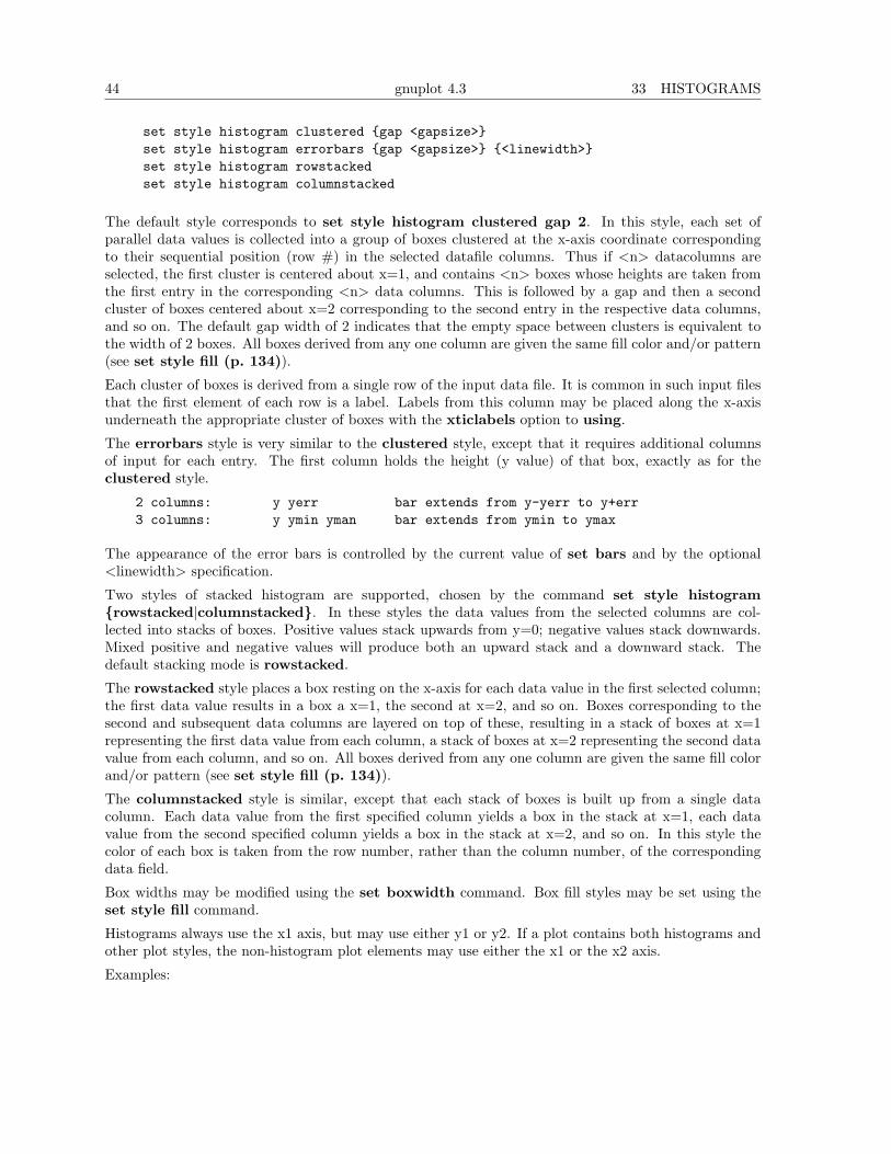
44 gnuplot 4.3 33 HISTOGRAMS
set style histogram clustered {gap <gapsize>}set style histogram errorbars {gap <gapsize>} {<linewidth>}set style histogram rowstackedset style histogram columnstacked
The default style corresponds to set style histogram clustered gap 2. In this style, each set ofparallel data values is collected into a group of boxes clustered at the x-axis coordinate correspondingto their sequential position (row #) in the selected datafile columns. Thus if <n> datacolumns areselected, the first cluster is centered about x=1, and contains <n> boxes whose heights are taken fromthe first entry in the corresponding <n> data columns. This is followed by a gap and then a secondcluster of boxes centered about x=2 corresponding to the second entry in the respective data columns,and so on. The default gap width of 2 indicates that the empty space between clusters is equivalent tothe width of 2 boxes. All boxes derived from any one column are given the same fill color and/or pattern(see set style fill (p. 134)).
Each cluster of boxes is derived from a single row of the input data file. It is common in such input filesthat the first element of each row is a label. Labels from this column may be placed along the x-axisunderneath the appropriate cluster of boxes with the xticlabels option to using.
The errorbars style is very similar to the clustered style, except that it requires additional columnsof input for each entry. The first column holds the height (y value) of that box, exactly as for theclustered style.
2 columns: y yerr bar extends from y-yerr to y+err3 columns: y ymin yman bar extends from ymin to ymax
The appearance of the error bars is controlled by the current value of set bars and by the optional<linewidth> specification.
Two styles of stacked histogram are supported, chosen by the command set style histogram{rowstacked|columnstacked}. In these styles the data values from the selected columns are col-lected into stacks of boxes. Positive values stack upwards from y=0; negative values stack downwards.Mixed positive and negative values will produce both an upward stack and a downward stack. Thedefault stacking mode is rowstacked.
The rowstacked style places a box resting on the x-axis for each data value in the first selected column;the first data value results in a box a x=1, the second at x=2, and so on. Boxes corresponding to thesecond and subsequent data columns are layered on top of these, resulting in a stack of boxes at x=1representing the first data value from each column, a stack of boxes at x=2 representing the second datavalue from each column, and so on. All boxes derived from any one column are given the same fill colorand/or pattern (see set style fill (p. 134)).
The columnstacked style is similar, except that each stack of boxes is built up from a single datacolumn. Each data value from the first specified column yields a box in the stack at x=1, each datavalue from the second specified column yields a box in the stack at x=2, and so on. In this style thecolor of each box is taken from the row number, rather than the column number, of the correspondingdata field.
Box widths may be modified using the set boxwidth command. Box fill styles may be set using theset style fill command.
Histograms always use the x1 axis, but may use either y1 or y2. If a plot contains both histograms andother plot styles, the non-histogram plot elements may use either the x1 or the x2 axis.
Examples:
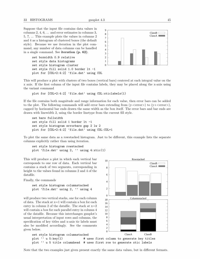
33 HISTOGRAMS gnuplot 4.3 45
0
1
2
3
4
5
6
7
8
9
ClassAClassB
Suppose that the input file contains data values incolumns 2, 4, 6, ... and error estimates in columns 3,5, 7, ... This example plots the values in columns 2and 4 as a histogram of clustered boxes (the defaultstyle). Because we use iteration in the plot com-mand, any number of data columns can be handledin a single command. See iteration (p. 62).
set boxwidth 0.9 relativeset style data histogramsset style histogram clusterset style fill solid 1.0 border lt -1plot for [COL=2:4:2] ’file.dat’ using COL
This will produce a plot with clusters of two boxes (vertical bars) centered at each integral value on thex axis. If the first column of the input file contains labels, they may be placed along the x-axis usingthe variant command
plot for [COL=2:4:2] ’file.dat’ using COL:xticlabels(1)
If the file contains both magnitude and range information for each value, then error bars can be addedto the plot. The following commands will add error bars extending from (y-<error>) to (y+<error>),capped by horizontal bar ends drawn the same width as the box itself. The error bars and bar ends aredrawn with linewidth 2, using the border linetype from the current fill style.
set bars fullwidthset style fill solid 1 border lt -1set style histogram errorbars gap 2 lw 2plot for [COL=2:4:2] ’file.dat’ using COL:COL+1
To plot the same data as a rowstacked histogram. Just to be different, this example lists the separatecolumns explicitly rather than using iteration.
set style histogram rowstackedplot ’file.dat’ using 2, ’’ using 4:xtic(1)
0
2
4
6
8
10 Rowstacked
ClassAClassB
This will produce a plot in which each vertical barcorresponds to one row of data. Each vertical barcontains a stack of two segments, corresponding inheight to the values found in columns 2 and 4 of thedatafile.
Finally, the commands
set style histogram columnstackedplot ’file.dat’ using 2, ’’ using 4
0 2 4 6 8
10 12 14 16 18
ClassA ClassB
Columnstackedwill produce two vertical stacks, one for each columnof data. The stack at x=1 will contain a box for eachentry in column 2 of the datafile. The stack at x=2will contain a box for each parallel entry in column 4of the datafile. Because this interchanges gnuplot’susual interpretation of input rows and columns, thespecification of key titles and x-axis tic labels mustalso be modified accordingly. See the commentsgiven below.
set style histogram columnstackedplot ’’ u 5:key(1) # uses first column to generate key titlesplot ’’ u 5 title columnhead # uses first row to generate xtic labels
Note that the two examples just given present exactly the same data values, but in different formats.
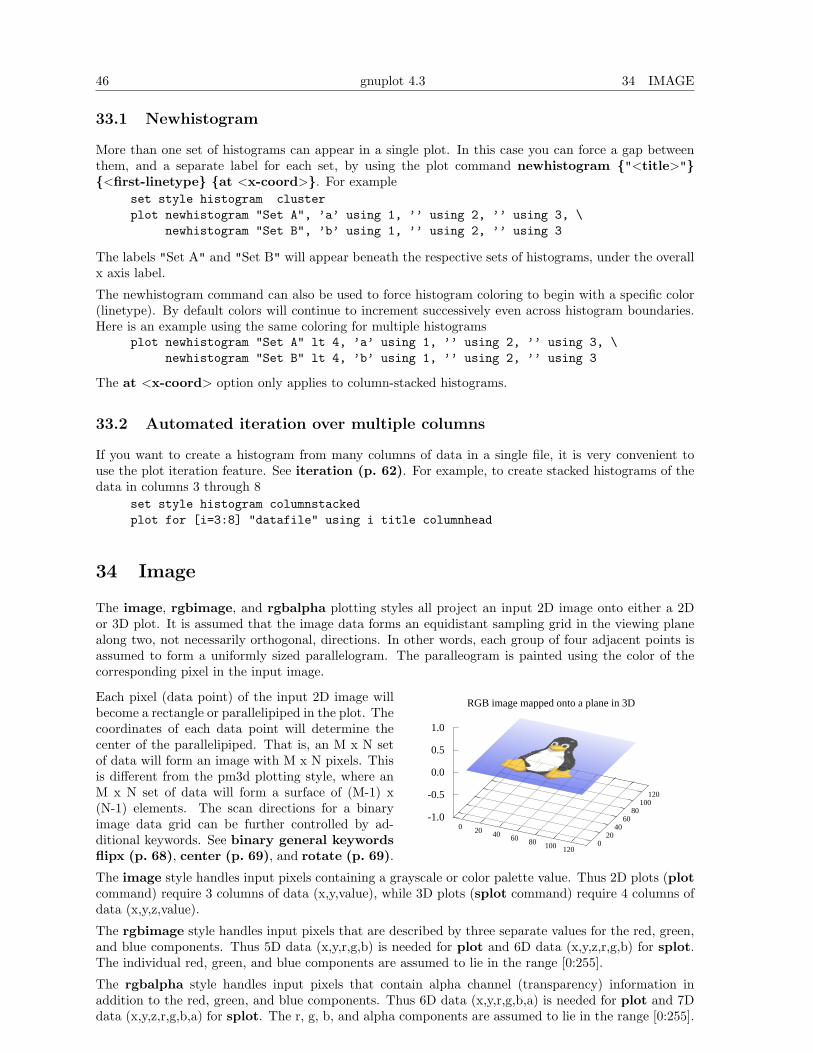
46 gnuplot 4.3 34 IMAGE
33.1 Newhistogram
More than one set of histograms can appear in a single plot. In this case you can force a gap betweenthem, and a separate label for each set, by using the plot command newhistogram {"<title>"}{<first-linetype} {at <x-coord>}. For example
set style histogram clusterplot newhistogram "Set A", ’a’ using 1, ’’ using 2, ’’ using 3, \
newhistogram "Set B", ’b’ using 1, ’’ using 2, ’’ using 3
The labels "Set A" and "Set B" will appear beneath the respective sets of histograms, under the overallx axis label.
The newhistogram command can also be used to force histogram coloring to begin with a specific color(linetype). By default colors will continue to increment successively even across histogram boundaries.Here is an example using the same coloring for multiple histograms
plot newhistogram "Set A" lt 4, ’a’ using 1, ’’ using 2, ’’ using 3, \newhistogram "Set B" lt 4, ’b’ using 1, ’’ using 2, ’’ using 3
The at <x-coord> option only applies to column-stacked histograms.
33.2 Automated iteration over multiple columns
If you want to create a histogram from many columns of data in a single file, it is very convenient touse the plot iteration feature. See iteration (p. 62). For example, to create stacked histograms of thedata in columns 3 through 8
set style histogram columnstackedplot for [i=3:8] "datafile" using i title columnhead
34 Image
The image, rgbimage, and rgbalpha plotting styles all project an input 2D image onto either a 2Dor 3D plot. It is assumed that the image data forms an equidistant sampling grid in the viewing planealong two, not necessarily orthogonal, directions. In other words, each group of four adjacent points isassumed to form a uniformly sized parallelogram. The paralleogram is painted using the color of thecorresponding pixel in the input image.
0 20 40 60 80 100 120 0
20 40
60 80
100 120
-1.0
-0.5
0.0
0.5
1.0
RGB image mapped onto a plane in 3DEach pixel (data point) of the input 2D image willbecome a rectangle or parallelipiped in the plot. Thecoordinates of each data point will determine thecenter of the parallelipiped. That is, an M x N setof data will form an image with M x N pixels. Thisis different from the pm3d plotting style, where anM x N set of data will form a surface of (M-1) x(N-1) elements. The scan directions for a binaryimage data grid can be further controlled by ad-ditional keywords. See binary general keywordsflipx (p. 68), center (p. 69), and rotate (p. 69).
The image style handles input pixels containing a grayscale or color palette value. Thus 2D plots (plotcommand) require 3 columns of data (x,y,value), while 3D plots (splot command) require 4 columns ofdata (x,y,z,value).
The rgbimage style handles input pixels that are described by three separate values for the red, green,and blue components. Thus 5D data (x,y,r,g,b) is needed for plot and 6D data (x,y,z,r,g,b) for splot.The individual red, green, and blue components are assumed to lie in the range [0:255].
The rgbalpha style handles input pixels that contain alpha channel (transparency) information inaddition to the red, green, and blue components. Thus 6D data (x,y,r,g,b,a) is needed for plot and 7Ddata (x,y,z,r,g,b,a) for splot. The r, g, b, and alpha components are assumed to lie in the range [0:255].
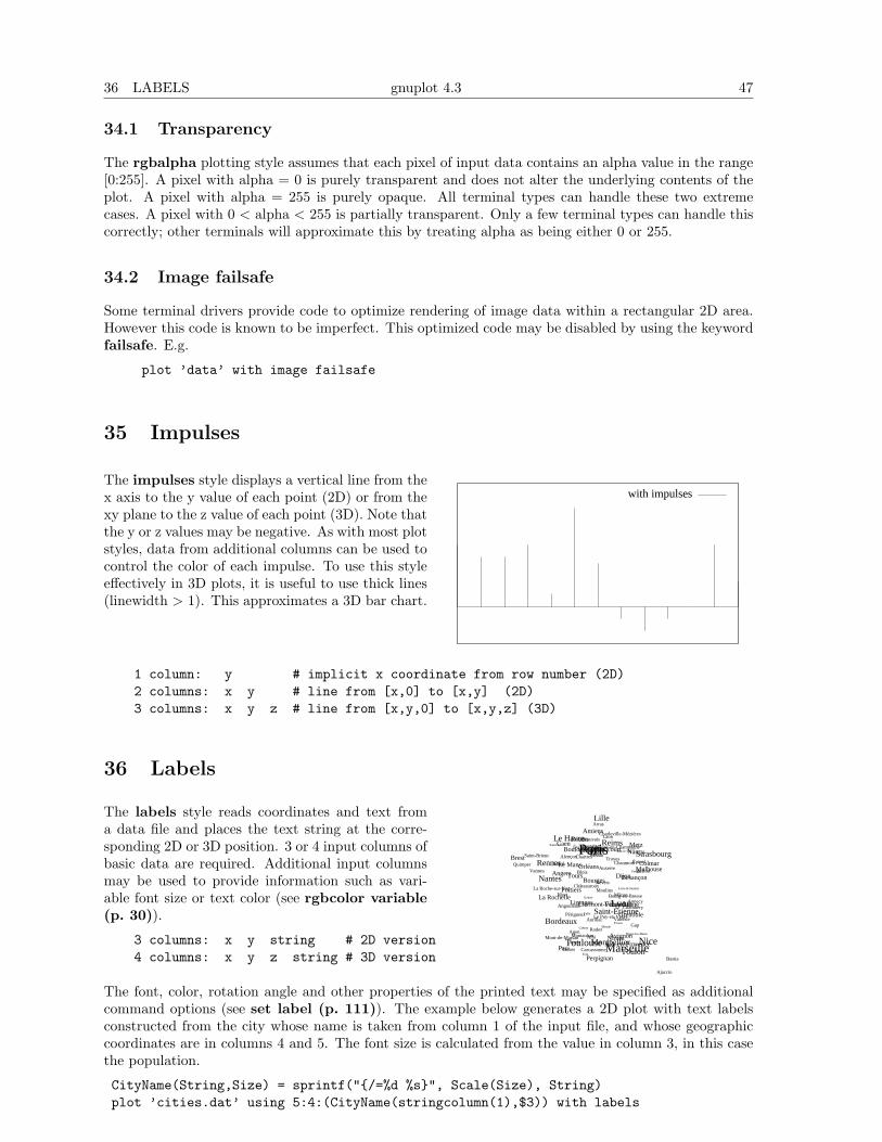
36 LABELS gnuplot 4.3 47
34.1 Transparency
The rgbalpha plotting style assumes that each pixel of input data contains an alpha value in the range[0:255]. A pixel with alpha = 0 is purely transparent and does not alter the underlying contents of theplot. A pixel with alpha = 255 is purely opaque. All terminal types can handle these two extremecases. A pixel with 0 < alpha < 255 is partially transparent. Only a few terminal types can handle thiscorrectly; other terminals will approximate this by treating alpha as being either 0 or 255.
34.2 Image failsafe
Some terminal drivers provide code to optimize rendering of image data within a rectangular 2D area.However this code is known to be imperfect. This optimized code may be disabled by using the keywordfailsafe. E.g.
plot ’data’ with image failsafe
35 Impulses
with impulsesThe impulses style displays a vertical line from thex axis to the y value of each point (2D) or from thexy plane to the z value of each point (3D). Note thatthe y or z values may be negative. As with most plotstyles, data from additional columns can be used tocontrol the color of each impulse. To use this styleeffectively in 3D plots, it is useful to use thick lines(linewidth > 1). This approximates a 3D bar chart.
1 column: y # implicit x coordinate from row number (2D)2 columns: x y # line from [x,0] to [x,y] (2D)3 columns: x y z # line from [x,y,0] to [x,y,z] (3D)
36 Labels
Paris
Marseille
Lyon
Toulouse Nice
Nantes
Strasbourg
Montpellier
Bordeaux
Rennes
Le Havre Reims
Lille
Saint-Étienne
Toulon
Grenoble
Angers
BrestLe Mans
Dijon
Aix-en-Provence
Clermont-Ferrand
Nîmes
Amiens
Tours
Limoges
Metz
Villeurbanne
Besançon
Caen
Orléans Mulhouse
Perpignan
Boulogne-Billancourt
Rouen
Nancy
Avignon
Nanterre
Poitiers
VersaillesCréteil
Pau
La Rochelle
Bourges
Colmar
Valence
QuimperTroyes
Chambéry
Niort
Charleville-MézièresBeauvais
Vannes
Montauban
Laval
Évreux
La Roche-sur-Yon
Belfort
Annecy
Blois
Châteauroux
Ajaccio
ÉvryChâlons-en-Champagne
Albi
Tarbes Carcassonne
Saint-Brieuc
Angoulême
Bobigny
Bourg-en-Bresse
Bastia
Arras
Nevers
Chartres
Auxerre
Gap
MelunÉpinal
Mâcon
Mont-de-MarsanAgen
PérigueuxAurillac
Alençon
Pontoise
Laon
Chaumont
Rodez
Auch
Moulins
Le Puy-en-Velay
Cahors
Saint-Lô
Lons-le-Saunier
Vesoul
Bar-le-Duc
Digne-les-Bains
Tulle
Guéret
MendePrivas
Foix
The labels style reads coordinates and text froma data file and places the text string at the corre-sponding 2D or 3D position. 3 or 4 input columns ofbasic data are required. Additional input columnsmay be used to provide information such as vari-able font size or text color (see rgbcolor variable(p. 30)).
3 columns: x y string # 2D version4 columns: x y z string # 3D version
The font, color, rotation angle and other properties of the printed text may be specified as additionalcommand options (see set label (p. 111)). The example below generates a 2D plot with text labelsconstructed from the city whose name is taken from column 1 of the input file, and whose geographiccoordinates are in columns 4 and 5. The font size is calculated from the value in column 3, in this casethe population.
CityName(String,Size) = sprintf("{/=%d %s}", Scale(Size), String)plot ’cities.dat’ using 5:4:(CityName(stringcolumn(1),$3)) with labels
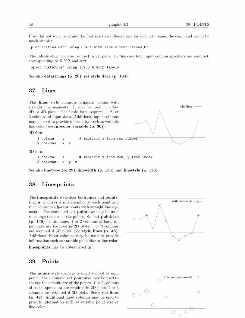
48 gnuplot 4.3 39 POINTS
If we did not want to adjust the font size to a different size for each city name, the command would bemuch simpler:
plot ’cities.dat’ using 5:4:1 with labels font "Times,8"
The labels style can also be used in 3D plots. In this case four input column specifiers are required,corresponding to X Y Z and text.
splot ’datafile’ using 1:2:3:4 with labels
See also datastrings (p. 20), set style data (p. 134).
37 Lines
with linesThe lines style connects adjacent points withstraight line segments. It may be used in either2D or 3D plots. The basic form requires 1, 2, or3 columns of input data. Additional input columnsmay be used to provide information such as variableline color (see rgbcolor variable (p. 30)).
2D form1 column: y # implicit x from row number2 columns: x y
3D form1 column: z # implicit x from row, y from index3 columns: x y z
See also linetype (p. 29), linewidth (p. 136), and linestyle (p. 136).
38 Linespoints
with linespointsThe linespoints style does both lines and points,that is, it draws a small symbol at each point andthen connects adjacent points with straight line seg-ments. The command set pointsize may be usedto change the size of the points. See set pointsize(p. 130) for its usage. 1 or 2 columns of basic in-put data are required in 2D plots; 1 or 3 columnsare required if 3D plots. See style lines (p. 48).Additional input columns may be used to provideinformation such as variable point size or line color.
linespoints may be abbreviated lp.
39 Points
with points ps variableThe points style displays a small symbol at eachpoint. The command set pointsize may be used tochange the default size of the points. 1 or 2 columnsof basic input data are required in 2D plots; 1 or 3columns are required if 3D plots. See style lines(p. 48). Additional input columns may be used toprovide information such as variable point size orline color.
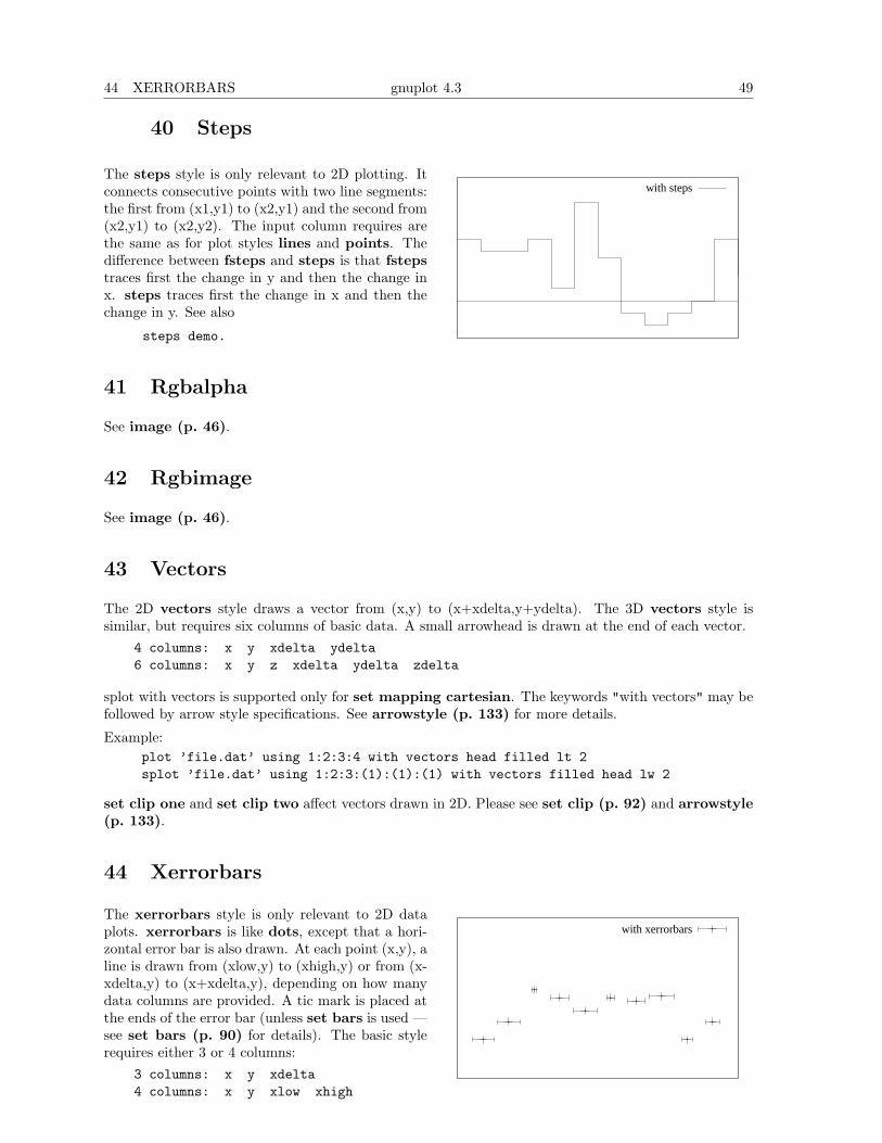
44 XERRORBARS gnuplot 4.3 49
40 Steps
with stepsThe steps style is only relevant to 2D plotting. Itconnects consecutive points with two line segments:the first from (x1,y1) to (x2,y1) and the second from(x2,y1) to (x2,y2). The input column requires arethe same as for plot styles lines and points. Thedifference between fsteps and steps is that fstepstraces first the change in y and then the change inx. steps traces first the change in x and then thechange in y. See also
steps demo.
41 Rgbalpha
See image (p. 46).
42 Rgbimage
See image (p. 46).
43 Vectors
The 2D vectors style draws a vector from (x,y) to (x+xdelta,y+ydelta). The 3D vectors style issimilar, but requires six columns of basic data. A small arrowhead is drawn at the end of each vector.
4 columns: x y xdelta ydelta6 columns: x y z xdelta ydelta zdelta
splot with vectors is supported only for set mapping cartesian. The keywords "with vectors" may befollowed by arrow style specifications. See arrowstyle (p. 133) for more details.
Example:plot ’file.dat’ using 1:2:3:4 with vectors head filled lt 2splot ’file.dat’ using 1:2:3:(1):(1):(1) with vectors filled head lw 2
set clip one and set clip two affect vectors drawn in 2D. Please see set clip (p. 92) and arrowstyle(p. 133).
44 Xerrorbars
with xerrorbarsThe xerrorbars style is only relevant to 2D dataplots. xerrorbars is like dots, except that a hori-zontal error bar is also drawn. At each point (x,y), aline is drawn from (xlow,y) to (xhigh,y) or from (x-xdelta,y) to (x+xdelta,y), depending on how manydata columns are provided. A tic mark is placed atthe ends of the error bar (unless set bars is used —see set bars (p. 90) for details). The basic stylerequires either 3 or 4 columns:
3 columns: x y xdelta4 columns: x y xlow xhigh
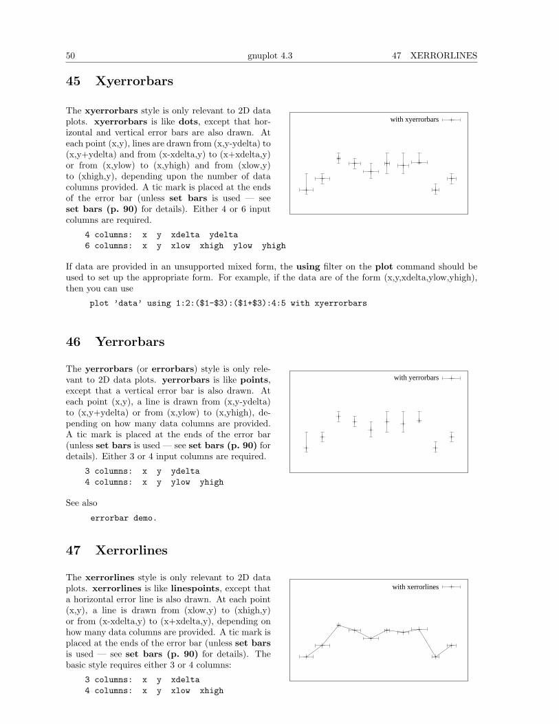
50 gnuplot 4.3 47 XERRORLINES
45 Xyerrorbars
with xyerrorbarsThe xyerrorbars style is only relevant to 2D dataplots. xyerrorbars is like dots, except that hor-izontal and vertical error bars are also drawn. Ateach point (x,y), lines are drawn from (x,y-ydelta) to(x,y+ydelta) and from (x-xdelta,y) to (x+xdelta,y)or from (x,ylow) to (x,yhigh) and from (xlow,y)to (xhigh,y), depending upon the number of datacolumns provided. A tic mark is placed at the endsof the error bar (unless set bars is used — seeset bars (p. 90) for details). Either 4 or 6 inputcolumns are required.
4 columns: x y xdelta ydelta6 columns: x y xlow xhigh ylow yhigh
If data are provided in an unsupported mixed form, the using filter on the plot command should beused to set up the appropriate form. For example, if the data are of the form (x,y,xdelta,ylow,yhigh),then you can use
plot ’data’ using 1:2:($1-$3):($1+$3):4:5 with xyerrorbars
46 Yerrorbars
with yerrorbarsThe yerrorbars (or errorbars) style is only rele-vant to 2D data plots. yerrorbars is like points,except that a vertical error bar is also drawn. Ateach point (x,y), a line is drawn from (x,y-ydelta)to (x,y+ydelta) or from (x,ylow) to (x,yhigh), de-pending on how many data columns are provided.A tic mark is placed at the ends of the error bar(unless set bars is used — see set bars (p. 90) fordetails). Either 3 or 4 input columns are required.
3 columns: x y ydelta4 columns: x y ylow yhigh
See also
errorbar demo.
47 Xerrorlines
with xerrorlinesThe xerrorlines style is only relevant to 2D dataplots. xerrorlines is like linespoints, except thata horizontal error line is also drawn. At each point(x,y), a line is drawn from (xlow,y) to (xhigh,y)or from (x-xdelta,y) to (x+xdelta,y), depending onhow many data columns are provided. A tic mark isplaced at the ends of the error bar (unless set barsis used — see set bars (p. 90) for details). Thebasic style requires either 3 or 4 columns:
3 columns: x y xdelta4 columns: x y xlow xhigh
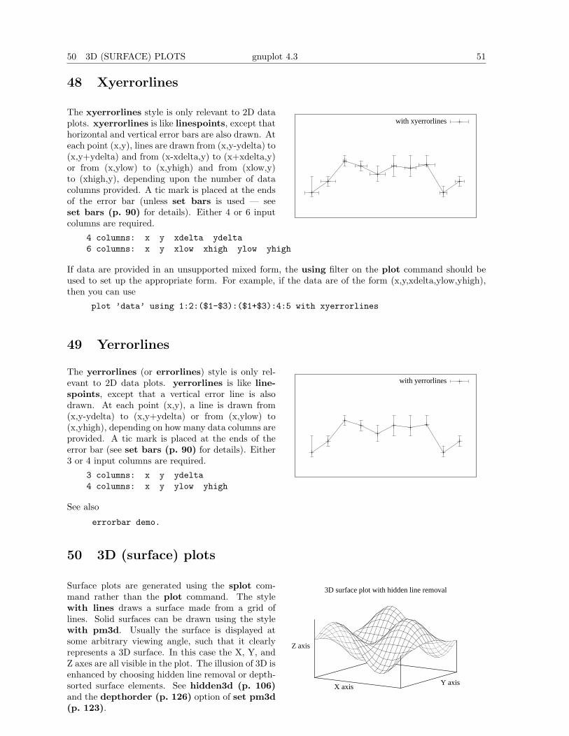
50 3D (SURFACE) PLOTS gnuplot 4.3 51
48 Xyerrorlines
with xyerrorlinesThe xyerrorlines style is only relevant to 2D dataplots. xyerrorlines is like linespoints, except thathorizontal and vertical error bars are also drawn. Ateach point (x,y), lines are drawn from (x,y-ydelta) to(x,y+ydelta) and from (x-xdelta,y) to (x+xdelta,y)or from (x,ylow) to (x,yhigh) and from (xlow,y)to (xhigh,y), depending upon the number of datacolumns provided. A tic mark is placed at the endsof the error bar (unless set bars is used — seeset bars (p. 90) for details). Either 4 or 6 inputcolumns are required.
4 columns: x y xdelta ydelta6 columns: x y xlow xhigh ylow yhigh
If data are provided in an unsupported mixed form, the using filter on the plot command should beused to set up the appropriate form. For example, if the data are of the form (x,y,xdelta,ylow,yhigh),then you can use
plot ’data’ using 1:2:($1-$3):($1+$3):4:5 with xyerrorlines
49 Yerrorlines
with yerrorlinesThe yerrorlines (or errorlines) style is only rel-evant to 2D data plots. yerrorlines is like line-spoints, except that a vertical error line is alsodrawn. At each point (x,y), a line is drawn from(x,y-ydelta) to (x,y+ydelta) or from (x,ylow) to(x,yhigh), depending on how many data columns areprovided. A tic mark is placed at the ends of theerror bar (see set bars (p. 90) for details). Either3 or 4 input columns are required.
3 columns: x y ydelta4 columns: x y ylow yhigh
See also
errorbar demo.
50 3D (surface) plots
3D surface plot with hidden line removal
X axisY axis
Z axis
Surface plots are generated using the splot com-mand rather than the plot command. The stylewith lines draws a surface made from a grid oflines. Solid surfaces can be drawn using the stylewith pm3d. Usually the surface is displayed atsome arbitrary viewing angle, such that it clearlyrepresents a 3D surface. In this case the X, Y, andZ axes are all visible in the plot. The illusion of 3D isenhanced by choosing hidden line removal or depth-sorted surface elements. See hidden3d (p. 106)and the depthorder (p. 126) option of set pm3d(p. 123).
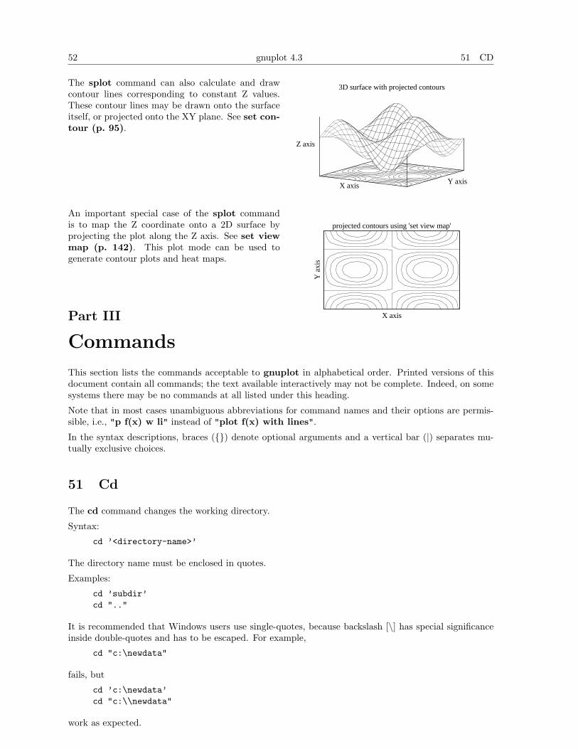
52 gnuplot 4.3 51 CD
3D surface with projected contours
X axisY axis
Z axis
The splot command can also calculate and drawcontour lines corresponding to constant Z values.These contour lines may be drawn onto the surfaceitself, or projected onto the XY plane. See set con-tour (p. 95).
projected contours using 'set view map'
X axisY
axi
s
An important special case of the splot commandis to map the Z coordinate onto a 2D surface byprojecting the plot along the Z axis. See set viewmap (p. 142). This plot mode can be used togenerate contour plots and heat maps.
Part III
Commands
This section lists the commands acceptable to gnuplot in alphabetical order. Printed versions of thisdocument contain all commands; the text available interactively may not be complete. Indeed, on somesystems there may be no commands at all listed under this heading.
Note that in most cases unambiguous abbreviations for command names and their options are permis-sible, i.e., "p f(x) w li" instead of "plot f(x) with lines".
In the syntax descriptions, braces ({}) denote optional arguments and a vertical bar (|) separates mu-tually exclusive choices.
51 Cd
The cd command changes the working directory.
Syntax:
cd ’<directory-name>’
The directory name must be enclosed in quotes.
Examples:
cd ’subdir’cd ".."
It is recommended that Windows users use single-quotes, because backslash [\] has special significanceinside double-quotes and has to be escaped. For example,
cd "c:\newdata"
fails, but
cd ’c:\newdata’cd "c:\\newdata"
work as expected.
54 EVALUATE gnuplot 4.3 53
52 Call
The call command is identical to the load command with one exception: you can have up to tenadditional parameters to the command (delimited according to the standard parser rules) which canbe substituted into the lines read from the file. As each line is read from the called input file, it isscanned for the sequence $ (dollar-sign) followed by a digit (0–9). If found, the sequence is replaced bythe corresponding parameter from the call command line. If the parameter was specified as a stringin the call line, it is substituted without its enclosing quotes. Sequence $# is replaced by the numberof passed parameters. $ followed by any character will be that character; e.g. use $$ to get a single$. Providing more than ten parameters on the call command line will cause an error. A parameterthat was not provided substitutes as nothing. Files being called may themselves contain call or loadcommands.
Syntax:call "<input-file>" <parameter-0> <parm-1> ... <parm-9>
The name of the input file must be enclosed in quotes, and it is recommended that parameters aresimilarly enclosed in quotes (future versions of gnuplot may treat quoted and unquoted argumentsdifferently).
Example:
If the file ’calltest.gp’ contains the line:print "argc=$# p0=$0 p1=$1 p2=$2 p3=$3 p4=$4 p5=$5 p6=$6 p7=x$7x"
entering the command:call ’calltest.gp’ "abcd" 1.2 + "’quoted’" -- "$2"
will display:argc=7 p0=abcd p1=1.2 p2=+ p3=’quoted’ p4=- p5=- p6=$2 p7=xx
NOTE: there is a clash in syntax with the datafile using callback operator. Use $$n or column(n) toaccess column n from a datafile inside a called datafile plot.
53 Clear
The clear command erases the current screen or output device as specified by set output. This usuallygenerates a formfeed on hardcopy devices. Use set terminal to set the device type.
For some terminals clear erases only the portion of the plotting surface defined by set size, so for theseit can be used in conjunction with set multiplot to create an inset.
Example:set multiplotplot sin(x)set origin 0.5,0.5set size 0.4,0.4clearplot cos(x)unset multiplot
Please see set multiplot (p. 117), set size (p. 132), and set origin (p. 121) for details of thesecommands.
54 Evaluate
The evaluate command executes the commands given as an argument string. Newline characters arenot allowed within the string.
Syntax:
54 gnuplot 4.3 56 FIT
eval <string expression>
This is especially useful for a repetition of similar commands.
Example:
set_label(x, y, text) \= sprintf("set label ’%s’ at %f, %f point pt 5", text, x, y)
eval set_label(1., 1., ’one/one’)eval set_label(2., 1., ’two/one’)eval set_label(1., 2., ’one/two’)
Please see substitution macros (p. 35) for another way to execute commands from a string.
55 Exit
The commands exit and quit, as well as the END-OF-FILE character (usually Ctrl-D) terminate inputfrom the current input stream: terminal session, pipe, and file input (pipe).
If input streams are nested (inherited load scripts), then reading will continue in the parent stream.When the top level stream is closed, the program itself will exit.
The command exit gnuplot will immediately and unconditionally cause gnuplot to exit even if the inputstream is multiply nested. In this case any open output files may not be completed cleanly. Example ofuse:
bind "ctrl-x" "unset output; exit gnuplot"
See help for batch/interactive (p. 18) for more details.
56 Fit
The fit command can fit a user-defined function to a set of data points (x,y) or (x,y,z), using an im-plementation of the nonlinear least-squares (NLLS) Marquardt-Levenberg algorithm. Any user-definedvariable occurring in the function body may serve as a fit parameter, but the return type of the functionmust be real.
Syntax:
fit {[xrange] {[yrange]}} <function> ’<datafile>’{datafile-modifiers}via ’<parameter file>’ | <var1>{,<var2>,...}
Ranges may be specified to temporarily limit the data which is to be fitted; any out-of-range data pointsare ignored. The syntax is
[{dummy_variable=}{<min>}{:<max>}],
analogous to plot; see plot ranges (p. 78).
<function> is any valid gnuplot expression, although it is usual to use a previously user-defined functionof the form f(x) or f(x,y).
<datafile> is treated as in the plot command. All the plot datafile modifiers (using, every,...) exceptsmooth and the deprecated thru are applicable to fit. See plot datafile (p. 64).
The default data formats for fitting functions with a single independent variable, y=f(x), are {x:}y orx:y:s; those formats can be changed with the datafile using qualifier. The third item (a column numberor an expression), if present, is interpreted as the standard deviation of the corresponding y value and isused to compute a weight for the datum, 1/s**2. Otherwise, all data points are weighted equally, witha weight of one. Note that if you don’t specify a using option at all, no y deviations are read from thedatafile even if it does have a third column, so you’ll always get unit weights.
56 FIT gnuplot 4.3 55
To fit a function with two independent variables, z=f(x,y), the required format is using with four items,x:y:z:s. The complete format must be given — no default columns are assumed for a missing token.Weights for each data point are evaluated from ’s’ as above. If error estimates are not available, aconstant value can be specified as a constant expression (see plot datafile using (p. 74)), e.g., using1:2:3:(1).
Multiple datasets may be simultaneously fit with functions of one independent variable by making y a’pseudo-variable’, e.g., the dataline number, and fitting as two independent variables. See fit multi-branch (p. 59).
The via qualifier specifies which parameters are to be adjusted, either directly, or by referencing aparameter file.
Examples:
f(x) = a*x**2 + b*x + cg(x,y) = a*x**2 + b*y**2 + c*x*yFIT_LIMIT = 1e-6fit f(x) ’measured.dat’ via ’start.par’fit f(x) ’measured.dat’ using 3:($7-5) via ’start.par’fit f(x) ’./data/trash.dat’ using 1:2:3 via a, b, cfit g(x,y) ’surface.dat’ using 1:2:3:(1) via a, b, c
After each iteration step, detailed information about the current state of the fit is written to the display.The same information about the initial and final states is written to a log file, "fit.log". This file is alwaysappended to, so as to not lose any previous fit history; it should be deleted or renamed as desired. Byusing the command set fit logfile, the name of the log file can be changed.
If gnuplot was built with this option, and you activated it using set fit errorvariables, the error foreach fitted parameter will be stored in a variable named like the parameter, but with " err" appended.Thus the errors can be used as input for further computations.
The fit may be interrupted by pressing Ctrl-C. After the current iteration completes, you have theoption to (1) stop the fit and accept the current parameter values, (2) continue the fit, (3) execute agnuplot command as specified by the environment variable FIT SCRIPT. The default for FIT SCRIPTis replot, so if you had previously plotted both the data and the fitting function in one graph, you candisplay the current state of the fit.
Once fit has finished, the update command may be used to store final values in a file for subsequentuse as a parameter file. See update (p. 158) for details.
56.1 Adjustable parameters
There are two ways that via can specify the parameters to be adjusted, either directly on the commandline or indirectly, by referencing a parameter file. The two use different means to set initial values.
Adjustable parameters can be specified by a comma-separated list of variable names after the viakeyword. Any variable that is not already defined is created with an initial value of 1.0. However, the fitis more likely to converge rapidly if the variables have been previously declared with more appropriatestarting values.
In a parameter file, each parameter to be varied and a corresponding initial value are specified, one perline, in the form
varname = value
Comments, marked by ’#’, and blank lines are permissible. The special form
varname = value # FIXED
means that the variable is treated as a ’fixed parameter’, initialized by the parameter file, but notadjusted by fit. For clarity, it may be useful to designate variables as fixed parameters so that theirvalues are reported by fit. The keyword # FIXED has to appear in exactly this form.
56 gnuplot 4.3 56 FIT
56.2 Short introduction
fit is used to find a set of parameters that ’best’ fits your data to your user-defined function. The fit isjudged on the basis of the sum of the squared differences or ’residuals’ (SSR) between the input datapoints and the function values, evaluated at the same places. This quantity is often called ’chisquare’(i.e., the Greek letter chi, to the power of 2). The algorithm attempts to minimize SSR, or more precisely,WSSR, as the residuals are ’weighted’ by the input data errors (or 1.0) before being squared; see fiterror estimates (p. 56) for details.
That’s why it is called ’least-squares fitting’. Let’s look at an example to see what is meant by ’non-linear’,but first we had better go over some terms. Here it is convenient to use z as the dependent variablefor user-defined functions of either one independent variable, z=f(x), or two independent variables,z=f(x,y). A parameter is a user-defined variable that fit will adjust, i.e., an unknown quantity in thefunction declaration. Linearity/non-linearity refers to the relationship of the dependent variable, z, tothe parameters which fit is adjusting, not of z to the independent variables, x and/or y. (To be technical,the second {and higher} derivatives of the fitting function with respect to the parameters are zero for alinear least-squares problem).
For linear least-squares (LLS), the user-defined function will be a sum of simple functions, not involvingany parameters, each multiplied by one parameter. NLLS handles more complicated functions in whichparameters can be used in a large number of ways. An example that illustrates the difference betweenlinear and nonlinear least-squares is the Fourier series. One member may be written as
z=a*sin(c*x) + b*cos(c*x).
If a and b are the unknown parameters and c is constant, then estimating values of the parameters is alinear least-squares problem. However, if c is an unknown parameter, the problem is nonlinear.
In the linear case, parameter values can be determined by comparatively simple linear algebra, in onedirect step. However LLS is a special case which is also solved along with more general NLLS problems bythe iterative procedure that gnuplot uses. fit attempts to find the minimum by doing a search. Each step(iteration) calculates WSSR with a new set of parameter values. The Marquardt-Levenberg algorithmselects the parameter values for the next iteration. The process continues until a preset criterion ismet, either (1) the fit has "converged" (the relative change in WSSR is less than FIT LIMIT), or (2)it reaches a preset iteration count limit, FIT MAXITER (see fit control variables (p. 58)). The fitmay also be interrupted and subsequently halted from the keyboard (see fit (p. 54)). The user variableFIT CONVERGED contains 1 if the previous fit command terminated due to convergence; it contains0 if the previous fit terminated for any other reason.
Often the function to be fitted will be based on a model (or theory) that attempts to describe or predictthe behaviour of the data. Then fit can be used to find values for the free parameters of the model, todetermine how well the data fits the model, and to estimate an error range for each parameter. See fiterror estimates (p. 56).
Alternatively, in curve-fitting, functions are selected independent of a model (on the basis of experienceas to which are likely to describe the trend of the data with the desired resolution and a minimum numberof parameters*functions.) The fit solution then provides an analytic representation of the curve.
However, if all you really want is a smooth curve through your data points, the smooth option to plotmay be what you’ve been looking for rather than fit.
56.3 Error estimates
In fit, the term "error" is used in two different contexts, data error estimates and parameter errorestimates.
Data error estimates are used to calculate the relative weight of each data point when determining theweighted sum of squared residuals, WSSR or chisquare. They can affect the parameter estimates, sincethey determine how much influence the deviation of each data point from the fitted function has onthe final values. Some of the fit output information, including the parameter error estimates, is moremeaningful if accurate data error estimates have been provided.
The ’statistical overview’ describes some of the fit output and gives some background for the ’practical
56 FIT gnuplot 4.3 57
guidelines’.
56.3.1 Statistical overview
The theory of non-linear least-squares (NLLS) is generally described in terms of a normal distributionof errors, that is, the input data is assumed to be a sample from a population having a given meanand a Gaussian (normal) distribution about the mean with a given standard deviation. For a sample ofsufficiently large size, and knowing the population standard deviation, one can use the statistics of thechisquare distribution to describe a "goodness of fit" by looking at the variable often called "chisquare".Here, it is sufficient to say that a reduced chisquare (chisquare/degrees of freedom, where degrees offreedom is the number of datapoints less the number of parameters being fitted) of 1.0 is an indicationthat the weighted sum of squared deviations between the fitted function and the data points is the sameas that expected for a random sample from a population characterized by the function with the currentvalue of the parameters and the given standard deviations.
If the standard deviation for the population is not constant, as in counting statistics where variance =counts, then each point should be individually weighted when comparing the observed sum of deviationsand the expected sum of deviations.
At the conclusion fit reports ’stdfit’, the standard deviation of the fit, which is the rms of the residuals,and the variance of the residuals, also called ’reduced chisquare’ when the data points are weighted.The number of degrees of freedom (the number of data points minus the number of fitted parameters) isused in these estimates because the parameters used in calculating the residuals of the datapoints wereobtained from the same data. These values are exported to the variables
FIT_NDF = Number of degrees of freedomFIT_WSSR = Weighted sum-of-squares residualFIT_STDFIT = sqrt(WSSR/NDF)
To estimate confidence levels for the parameters, one can use the minimum chisquare obtained from thefit and chisquare statistics to determine the value of chisquare corresponding to the desired confidencelevel, but considerably more calculation is required to determine the combinations of parameters whichproduce such values.
Rather than determine confidence intervals, fit reports parameter error estimates which are readilyobtained from the variance-covariance matrix after the final iteration. By convention, these estimatesare called "standard errors" or "asymptotic standard errors", since they are calculated in the same wayas the standard errors (standard deviation of each parameter) of a linear least-squares problem, eventhough the statistical conditions for designating the quantity calculated to be a standard deviation arenot generally valid for the NLLS problem. The asymptotic standard errors are generally over-optimisticand should not be used for determining confidence levels, but are useful for qualitative purposes.
The final solution also produces a correlation matrix, which gives an indication of the correlation of pa-rameters in the region of the solution; if one parameter is changed, increasing chisquare, does changinganother compensate? The main diagonal elements, autocorrelation, are all 1; if all parameters were in-dependent, all other elements would be nearly 0. Two variables which completely compensate each otherwould have an off-diagonal element of unit magnitude, with a sign depending on whether the relationis proportional or inversely proportional. The smaller the magnitudes of the off-diagonal elements, thecloser the estimates of the standard deviation of each parameter would be to the asymptotic standarderror.
56.3.2 Practical guidelines
If you have a basis for assigning weights to each data point, doing so lets you make use of additionalknowledge about your measurements, e.g., take into account that some points may be more reliable thanothers. That may affect the final values of the parameters.
Weighting the data provides a basis for interpreting the additional fit output after the last iteration.Even if you weight each point equally, estimating an average standard deviation rather than using aweight of 1 makes WSSR a dimensionless variable, as chisquare is by definition.
58 gnuplot 4.3 56 FIT
Each fit iteration will display information which can be used to evaluate the progress of the fit. (An ’*’indicates that it did not find a smaller WSSR and is trying again.) The ’sum of squares of residuals’,also called ’chisquare’, is the WSSR between the data and your fitted function; fit has minimized that.At this stage, with weighted data, chisquare is expected to approach the number of degrees of freedom(data points minus parameters). The WSSR can be used to calculate the reduced chisquare (WSSR/ndf)or stdfit, the standard deviation of the fit, sqrt(WSSR/ndf). Both of these are reported for the finalWSSR.
If the data are unweighted, stdfit is the rms value of the deviation of the data from the fitted function,in user units.
If you supplied valid data errors, the number of data points is large enough, and the model is correct,the reduced chisquare should be about unity. (For details, look up the ’chi-squared distribution’ in yourfavourite statistics reference.) If so, there are additional tests, beyond the scope of this overview, fordetermining how well the model fits the data.
A reduced chisquare much larger than 1.0 may be due to incorrect data error estimates, data errorsnot normally distributed, systematic measurement errors, ’outliers’, or an incorrect model function. Aplot of the residuals, e.g., plot ’datafile’ using 1:($2-f($1)), may help to show any systematic trends.Plotting both the data points and the function may help to suggest another model.
Similarly, a reduced chisquare less than 1.0 indicates WSSR is less than that expected for a randomsample from the function with normally distributed errors. The data error estimates may be too large,the statistical assumptions may not be justified, or the model function may be too general, fittingfluctuations in a particular sample in addition to the underlying trends. In the latter case, a simplerfunction may be more appropriate.
You’ll have to get used to both fit and the kind of problems you apply it to before you can relate thestandard errors to some more practical estimates of parameter uncertainties or evaluate the significanceof the correlation matrix.
Note that fit, in common with most NLLS implementations, minimizes the weighted sum of squareddistances (y-f(x))**2. It does not provide any means to account for "errors" in the values of x, only in y.Also, any "outliers" (data points outside the normal distribution of the model) will have an exaggeratedeffect on the solution.
56.4 Control
There are a number of gnuplot variables that can be defined to affect fit. Those which can be definedonce gnuplot is running are listed under ’control variables’ while those defined before starting gnuplotare listed under ’environment variables’.
56.4.1 Control variables
The default epsilon limit (1e-5) may be changed by declaring a value forFIT_LIMIT
When the sum of squared residuals changes between two iteration steps by a factor less than this number(epsilon), the fit is considered to have ’converged’.
The maximum number of iterations may be limited by declaring a value forFIT_MAXITER
A value of 0 (or not defining it at all) means that there is no limit.
If you need even more control about the algorithm, and know the Marquardt-Levenberg algorithm well,there are some more variables to influence it. The startup value of lambda is normally calculatedautomatically from the ML-matrix, but if you want to, you may provide your own one with
FIT_START_LAMBDA
Specifying FIT START LAMBDA as zero or less will re-enable the automatic selection. The variableFIT_LAMBDA_FACTOR
56 FIT gnuplot 4.3 59
gives the factor by which lambda is increased or decreased whenever the chi-squared target functionincreased or decreased significantly. Setting FIT LAMBDA FACTOR to zero re-enables the defaultfactor of 10.0.
Other variables with the FIT prefix may be added to fit, so it is safer not to use that prefix foruser-defined variables.
The variables FIT SKIP and FIT INDEX were used by earlier releases of gnuplot with a ’fit’ patchcalled gnufit and are no longer available. The datafile every modifier provides the functionality ofFIT SKIP. FIT INDEX was used for multi-branch fitting, but multi-branch fitting of one independentvariable is now done as a pseudo-3D fit in which the second independent variable and using are used tospecify the branch. See fit multi-branch (p. 59).
56.4.2 Environment variables
The environment variables must be defined before gnuplot is executed; how to do so depends on youroperating system.
FIT_LOG
changes the name (and/or path) of the file to which the fit log will be written from the default of "fit.log"in the working directory. The default value can be overwritten using the command set fit logfile.
FIT_SCRIPT
specifies a command that may be executed after an user interrupt. The default is replot, but a plot orload command may be useful to display a plot customized to highlight the progress of the fit.
56.5 Multi-branch
In multi-branch fitting, multiple data sets can be simultaneously fit with functions of one indepen-dent variable having common parameters by minimizing the total WSSR. The function and parameters(branch) for each data set are selected by using a ’pseudo-variable’, e.g., either the dataline number (a’column’ index of -1) or the datafile index (-2), as the second independent variable.
Example: Given two exponential decays of the form, z=f(x), each describing a different data set buthaving a common decay time, estimate the values of the parameters. If the datafile has the format x:z:s,then
f(x,y) = (y==0) ? a*exp(-x/tau) : b*exp(-x/tau)fit f(x,y) ’datafile’ using 1:-2:2:3 via a, b, tau
For a more complicated example, see the file "hexa.fnc" used by the "fit.dem" demo.
Appropriate weighting may be required since unit weights may cause one branch to predominate if thereis a difference in the scale of the dependent variable. Fitting each branch separately, using the multi-branch solution as initial values, may give an indication as to the relative effect of each branch on thejoint solution.
56.6 Starting values
Nonlinear fitting is not guaranteed to converge to the global optimum (the solution with the smallestsum of squared residuals, SSR), and can get stuck at a local minimum. The routine has no way todetermine that; it is up to you to judge whether this has happened.
fit may, and often will get "lost" if started far from a solution, where SSR is large and changing slowlyas the parameters are varied, or it may reach a numerically unstable region (e.g., too large a numbercausing a floating point overflow) which results in an "undefined value" message or gnuplot halting.
To improve the chances of finding the global optimum, you should set the starting values at least roughlyin the vicinity of the solution, e.g., within an order of magnitude, if possible. The closer your startingvalues are to the solution, the less chance of stopping at another minimum. One way to find starting
60 gnuplot 4.3 57 HELP
values is to plot data and the fitting function on the same graph and change parameter values and replotuntil reasonable similarity is reached. The same plot is also useful to check whether the fit stopped at aminimum with a poor fit.
Of course, a reasonably good fit is not proof there is not a "better" fit (in either a statistical sense,characterized by an improved goodness-of-fit criterion, or a physical sense, with a solution more consistentwith the model.) Depending on the problem, it may be desirable to fit with various sets of startingvalues, covering a reasonable range for each parameter.
56.7 Tips
Here are some tips to keep in mind to get the most out of fit. They’re not very organized, so you’ll haveto read them several times until their essence has sunk in.
The two forms of the via argument to fit serve two largely distinct purposes. The via "file" form isbest used for (possibly unattended) batch operation, where you just supply the startup values in a fileand can later use update to copy the results back into another (or the same) parameter file.
The via var1, var2, ... form is best used interactively, where the command history mechanism maybe used to edit the list of parameters to be fitted or to supply new startup values for the next try. Thisis particularly useful for hard problems, where a direct fit to all parameters at once won’t work withoutgood starting values. To find such, you can iterate several times, fitting only some of the parameters,until the values are close enough to the goal that the final fit to all parameters at once will work.
Make sure that there is no mutual dependency among parameters of the function you are fitting. Forexample, don’t try to fit a*exp(x+b), because a*exp(x+b)=a*exp(b)*exp(x). Instead, fit either a*exp(x)or exp(x+b).
A technical issue: the parameters must not be too different in magnitude. The larger the ratio of thelargest and the smallest absolute parameter values, the slower the fit will converge. If the ratio is closeto or above the inverse of the machine floating point precision, it may take next to forever to converge,or refuse to converge at all. You will have to adapt your function to avoid this, e.g., replace ’parameter’by ’1e9*parameter’ in the function definition, and divide the starting value by 1e9.
If you can write your function as a linear combination of simple functions weighted by the parametersto be fitted, by all means do so. That helps a lot, because the problem is no longer nonlinear and shouldconverge with only a small number of iterations, perhaps just one.
Some prescriptions for analysing data, given in practical experimentation courses, may have you firstfit some functions to your data, perhaps in a multi-step process of accounting for several aspects ofthe underlying theory one by one, and then extract the information you really wanted from the fittingparameters of those functions. With fit, this may often be done in one step by writing the model functiondirectly in terms of the desired parameters. Transforming data can also quite often be avoided, thoughsometimes at the cost of a more difficult fit problem. If you think this contradicts the previous paragraphabout simplifying the fit function, you are correct.
A "singular matrix" message indicates that this implementation of the Marquardt-Levenberg algorithmcan’t calculate parameter values for the next iteration. Try different starting values, writing the functionin another form, or a simpler function.
Finally, a nice quote from the manual of another fitting package (fudgit), that kind of summarizes allthese issues: "Nonlinear fitting is an art!"
57 Help
The help command displays built-in help. To specify information on a particular topic use the syntax:
help {<topic>}
If <topic> is not specified, a short message is printed about gnuplot. After help for the requestedtopic is given, a menu of subtopics is given; help for a subtopic may be requested by typing its name,
59 IF gnuplot 4.3 61
extending the help request. After that subtopic has been printed, the request may be extended again oryou may go back one level to the previous topic. Eventually, the gnuplot command line will return.
If a question mark (?) is given as the topic, the list of topics currently available is printed on the screen.
58 History
history command lists or saves previous entries in the history of the command line editing, or executesan entry.
Here you find ’usage by examples’:history # show the complete historyhistory 5 # show last 5 entries in the historyhistory quiet 5 # show last 5 entries without entry numbershistory "hist.gp" # write the complete history to file hist.gphistory "hist.gp" append # append the complete history to file hist.gphistory 10 "hist.gp" # write last 10 commands to file hist.gphistory 10 "|head -5 >>diary.gp" # write 5 history commands using pipehistory ?load # show all history entries starting with "load"history ?"set c" # like above, several words enclosed in quoteshi !reread # execute last entry starting with "reread"hist !"set xr" # like above, several words enclosed in quoteshi !hi # guess yourself :-))
On systems which support a popen function (Unix), the output of history can be piped through anexternal program by starting the file name with a ’|’, as one of the above examples demonstrates.
59 If
The if command allows commands to be executed conditionally.
Syntax:if (<condition>) <command-line> [; else if (<condition>) ...; else ...]
<condition> will be evaluated. If it is true (non-zero), then the command(s) of the <command-line>will be executed. If <condition> is false (zero), then the entire <command-line> is ignored until thenext occurrence of else. Note that use of ; to allow multiple commands on the same line will not endthe conditionalized commands.
Examples:pi=3if (pi!=acos(-1)) print "?Fixing pi!"; pi=acos(-1); print pi
will display:?Fixing pi!3.14159265358979
butif (1==2) print "Never see this"; print "Or this either"
will not display anything.
else:v=0v=v+1; if (v%2) print "2" ; else if (v%3) print "3"; else print "fred"
(repeat the last line repeatedly!)
See reread (p. 84) for an example of how if (p. 61) and reread (p. 84) can be used together toperform a loop.
62 gnuplot 4.3 62 LOWER
60 Iteration
The plot, splot, set and unset commands may optionally contain an iteration clause. This has theeffect of executing the basic command multiple times, each time re-evaluating any expressions that makeuse of the iteration control variable. Two forms of iteration clause are currently supported:
for [intvar = start:end{:increment}]for [stringvar in "A B C D"]
Examples:
plot for [filename in "A.dat B.dat C.dat"] filename using 1:2 with linesplot for [basename in "A B C"] basename.".dat" using 1:2 with linesset for [i = 1:10] style line i lc rgb "blue"unset for [tag = 100:200] label tag
See additional documentation for plot iteration (p. 79).
61 Load
The load command executes each line of the specified input file as if it had been typed in interactively.Files created by the save command can later be loaded. Any text file containing valid commands canbe created and then executed by the load command. Files being loaded may themselves contain loador call commands. See comments (p. 19) for information about comments in commands. To loadwith arguments, see call (p. 53).
Syntax:load "<input-file>"
The name of the input file must be enclosed in quotes.
The special filename "-" may be used to load commands from standard input. This allows a gnuplotcommand file to accept some commands from standard input. Please see help for batch/interactive(p. 18) for more details.
On some systems which support a popen function (Unix), the load file can be read from a pipe bystarting the file name with a ’<’.
Examples:load ’work.gnu’load "func.dat"load "< loadfile_generator.sh"
The load command is performed implicitly on any file names given as arguments to gnuplot. Theseare loaded in the order specified, and then gnuplot exits.
62 Lower
Syntax:lower {plot_window_nb}
The lower command lowers (opposite to raise) plot window(s) associated with the interactive terminalof your gnuplot session, i.e. pm, win, wxt or x11. It puts the plot window to bottom in the z-orderwindows stack of the window manager of your desktop.
As x11 and wxt support multiple plot windows, then by default they lower these windows in descendingorder of most recently created on top to the least recently created on bottom. If a plot number is suppliedas an optional parameter, only the associated plot window will be lowered if it exists.
The optional parameter is ignored for single plot-window terminals, i.e. pm and win.
64 PLOT gnuplot 4.3 63
63 Pause
The pause command displays any text associated with the command and then waits a specified amountof time or until the carriage return is pressed. pause is especially useful in conjunction with load files.
Syntax:
pause <time> {"<string>"}pause mouse {<endcondition>}{, <endcondition>} {"<string>"}
<time> may be any constant or expression. Choosing -1 will wait until a carriage return is hit, zero (0)won’t pause at all, and a positive number will wait the specified number of seconds. The time is roundedto an integer number of seconds if subsecond time resolution is not supported by the given platform.pause 0 is synonymous with print.
If the current terminal supports mousing, then pause mouse will terminate on either a mouse click oron ctrl-C. For all other terminals, or if mousing is not active, pause mouse is equivalent to pause -1.
If one or more end conditions are given after pause mouse, then any one of the conditions will terminatethe pause. The possible end conditions are keypress, button1, button2, button3, close, and any. Ifthe pause terminates on a keypress, then the ascii value of the key pressed is returned in MOUSE KEY.The character itself is returned as a one character string in MOUSE CHAR. Hotkeys (bind command)are disabled if keypress is one of the end conditions. Zooming is disabled if button3 is one of the endconditions.
In all cases the coordinates of the mouse are returned in variables MOUSE X, MOUSE Y, MOUSE X2,MOUSE Y2. See mouse variables (p. 33).
Note: Since pause communicates with the operating system rather than the graphics, it may behavedifferently with different device drivers (depending upon how text and graphics are mixed).
Examples:
pause -1 # Wait until a carriage return is hitpause 3 # Wait three secondspause -1 "Hit return to continue"pause 10 "Isn’t this pretty? It’s a cubic spline."pause mouse "Click any mouse button on selected data point"pause mouse keypress "Type a letter from A-F in the active window"pause mouse button1,keypresspause mouse any "Any key or button will terminate"
The variant "pause mouse key" will resume after any keypress in the active plot window. If you wantto wait for a particular key to be pressed, you can use a reread loop such as:
print "I will resume after you hit the Tab key in the plot window"load "wait_for_tab"
File "wait for tab" contains the lines
pause mouse keyif (MOUSE_KEY != 9) reread
64 Plot
plot is the primary command for drawing plots with gnuplot. It creates plots of functions and datain many, many ways. plot is used to draw 2-d functions and data; splot draws 2D projections of 3Dsurfaces and data. plot and splot contain many common features; see splot (p. 153) for differences.Note specifically that although the binary <binary list> variation does work for both plot and splot,there are small differences between these modes.
Syntax:
64 gnuplot 4.3 64 PLOT
plot {<ranges>}{<iteration>}{<function> | {"<datafile>" {datafile-modifiers}}}{axes <axes>} {<title-spec>} {with <style>}{, {definitions,} <function> ...}
where either a <function> or the name of a data file enclosed in quotes is supplied. A function is amathematical expression or a pair of mathematical expressions in parametric mode. The expressionsmay be defined completely or in part earlier in the stream of gnuplot commands (see user-defined(p. 28)).
It is also possible to define functions and parameters on the plot command itself. This is done merelyby isolating them from other items with commas.
Examples:
plot sin(x)plot sin(x), cos(x)plot f(x) = sin(x*a), a = .2, f(x), a = .4, f(x)plot "datafile.1" with lines, "datafile.2" with pointsplot [t=1:10] [-pi:pi*2] tan(t), \
"data.1" using (tan($2)):($3/$4) smooth csplines \axes x1y2 notitle with lines 5
plot for [datafile in "spinach.dat broccoli.dat"] datafile
See also show plot (p. 122).
64.1 Axes
There are four possible sets of axes available; the keyword <axes> is used to select the axes for which aparticular line should be scaled. x1y1 refers to the axes on the bottom and left; x2y2 to those on thetop and right; x1y2 to those on the bottom and right; and x2y1 to those on the top and left. Rangesspecified on the plot command apply only to the first set of axes (bottom left).
64.2 Data
Discrete data contained in a file can be displayed by specifying the name of the data file (enclosed insingle or double quotes) on the plot command line.
Syntax:
plot ’<file_name>’ {binary <binary list>}{matrix}{index <index list> | index "<name>"}{every <every list>}{thru <thru expression>}{using <using list>}{smooth <option>}{volatile} {noautoscale}
The modifiers binary, index, every, thru, using, and smooth are discussed separately. In brief,binary allows data entry from a binary file (default is ASCII), index selects which data sets in a multi-data-set file are to be plotted, every specifies which points within a single data set are to be plotted,using determines how the columns within a single record are to be interpreted (thru is a special caseof using), and smooth allows for simple interpolation and approximation. (splot has a similar syntax,but does not support the smooth and thru options.)
The volatile keyword indicates that the contents of the data file may be different if the file is re-read.This tells the program to use refresh rather than replot commands whenever possible. See refresh(p. 83).
64 PLOT gnuplot 4.3 65
The noautoscale keyword means that the points making up this plot will be ignored when automaticallydetermining axis range limits.
ASCII DATA FILES:
Data files should contain at least one data point per record (using can select one data point from therecord). Records beginning with # (and also with ! on VMS) will be treated as comments and ignored.Each data point represents an (x,y) pair. For plots with error bars or error bars with lines (see set styleerrorbars (p. 50) or set style errorlines (p. 51)), each data point is (x,y,ydelta), (x,y,ylow,yhigh),(x,y,xdelta), (x,y,xlow,xhigh), or (x,y,xlow,xhigh,ylow,yhigh).
In all cases, the numbers of each record of a data file must be separated by white space (one or moreblanks or tabs) unless a format specifier is provided by the using option. This white space divideseach record into columns. However, whitespace inside a pair of double quotes is ignored when countingcolumns, so the following datafile line has three columns:
1.0 "second column" 3.0
Data may be written in exponential format with the exponent preceded by the letter e or E. The fortranexponential specifiers d, D, q, and Q may also be used if the command set datafile fortran is in effect.
Only one column (the y value) need be provided. If x is omitted, gnuplot provides integer valuesstarting at 0.
In datafiles, blank records (records with no characters other than blanks and a newline and/or carriagereturn) are significant.
Single blank records designate discontinuities in a plot; no line will join points separated by a blankrecords (if they are plotted with a line style).
Two blank records in a row indicate a break between separate data sets. See index (p. 71).
If autoscaling has been enabled (set autoscale), the axes are automatically extended to include alldatapoints, with a whole number of tic marks if tics are being drawn. This has two consequences: i) Forsplot, the corner of the surface may not coincide with the corner of the base. In this case, no verticalline is drawn. ii) When plotting data with the same x range on a dual-axis graph, the x coordinates maynot coincide if the x2tics are not being drawn. This is because the x axis has been autoextended to awhole number of tics, but the x2 axis has not. The following example illustrates the problem:
reset; plot ’-’, ’-’ axes x2y11 119 19e1 119 19e
To avoid this, you can use the fixmin/fixmax feature of the set autoscale command, which turns offthe automatic extension of the axis range upto the next tic mark.
Label coordinates and text can also be read from a data file (see labels (p. 47)).
BINARY DATA FILES:
Gnuplot can read binary data files. However, adequate information about details of the file formatmust be given on the command line or extracted from the file itself for a supported binary filetype. Inparticular, there are two structures for binary files, a matrix binary format and a general binary format.
The matrix binary format contains a two dimensional array of 32 bit IEEE float values with an additionalcolumn and row of coordinate values. As with ASCII matrix, in the using list, repetition of thecoordinate row constitutes column 1, repetition of the coordinate column constitutes column 2, and thearray of values constitutes column 3.
The general binary format contains an arbitrary number of columns for which information must bespecified at the command line. For example, array, record, format and using can indicate the size,format and dimension of data. There are a variety of useful commands for skipping file headers andchanging endianess. There are a set of commands for positioning and translating data since often
66 gnuplot 4.3 64 PLOT
coordinates are not part of the file when uniform sampling is inherent in the data. Different from matrixbinary or ASCII, general binary does not treat the generated columns as 1, 2 or 3 in the using list.Rather, column 1 begins with column 1 of the file, or as specified in the format list.
There are global default settings for the various binary options which may be set using the same syntaxas the options when used as part of the (s)plot <filename> binary ... command. This syntax isset datafile binary .... The general rule is that common command-line specified parameters overridefile-extracted parameters which override default parameters.
Matrix binary is the default binary format when no keywords specific to general binary are given, i.e.,array, record, format, filetype.
General binary data can be entered at the command line via the special file name ’-’. However, this isintended for use through a pipe where programs can exchange binary data, not for keyboards. There isno "end of record" character for binary data. Gnuplot continues reading from a pipe until it has readthe number of points declared in the array qualifier.
See datafile binary (p. 66) for more details.
64.2.1 Binary
The binary keyword allows a data file to be binary as opposed to ASCII. There are two formats forbinary–matrix binary and general binary. Matrix binary is a fixed format in which data appears in a 2Darray with an extra row and column for coordinate values. General binary is a flexible format for whichdetails about the file must be given at the command line.
See binary matrix (p. 154) or binary general (p. 66) for more details.
64.2.2 Binary general
General binary data in which format information is not necessarily part of the file can be read by givingfurther details about the file format at the command line. Although the syntax is slightly arcane tothe casual user, general binary is particularly useful for application programs using gnuplot and sendinglarge amounts of data.
Syntax:plot ’<file_name>’ {binary <binary list>} ...splot ’<file_name>’ {binary <binary list>} ...
General binary format is activated by keywords in <binary list> pertaining to information about filestructure, i.e., array, record, format or filetype. Otherwise, matrix binary format is assumed. (Seebinary matrix (p. 154) for more details.)
There are some standard file types that may be read for which details about the binary format maybe extracted automatically. (Type show datafile binary at the command line for a list.) Otherwise,details must be specified at the command line or set in the defaults. Keywords are described below.
The keyword filetype in <binary list> controls the routine used to read the file, i.e., the format of thedata. For a list of the supported file types, type show datafile binary filetypes. If no file type isgiven, the rule is that traditional gnuplot binary is assumed for splot if the binary keyword standsalone. In all other circumstances, for plot or when one of the <binary list> keywords appears, a rawbinary file is assumed whereby the keywords specify the binary format.
General binary data files fall into two basic classes, and some files may be of both classes depending uponhow they are treated. There is that class for which uniform sampling is assumed and point coordinatesmust be generated. This is the class for which full control via the <binary list> keywords applies. Forthis class, the settings precedence is that command line parameters override in-file parameters, whichoverride default settings. The other class is that set of files for which coordinate information is containedwithin the file or there is possibly a non-uniform sampling such as gnuplot binary.
Other than for the unique data files such as gnuplot binary, one should think of binary data as conceptu-ally the same as ASCII data. Each point has columns of information which are selected via the <usinglist> associated with using. When no format string is specified, gnuplot will retrieve a number of
64 PLOT gnuplot 4.3 67
binary variables equal to the largest column given in the <using list>. For example, using 1:3 willresult in three columns being read, of which the second will be ignored. There are default using listsbased upon the typical number of parameters associated with a certain plot type. For example, withimage has a default of using 1, while with rgbimage has a default of using 1:2:3. Note that thespecial characters for using representing point/line/index generally should not be used for binary data.There are keywords in <binary list> that control this.
64.2.2.1 Array Describes the sampling array dimensions associated with the binary file. The coor-dinates will be generated by gnuplot. A number must be specified for each dimension of the array. Forexample, array=(10,20) means the underlying sampling structure is two-dimensional with 10 pointsalong the first (x) dimension and 20 points along the second (y) dimension. A negative number indi-cates that data should be read until the end of file. If there is only one dimension, the parenthesesmay be omitted. A colon can be used to separate the dimensions for multiple records. For example,array=25:35 indicates there are two one-dimensional records in the file.
Note: Gnuplot version 4.2 used the syntax array=128x128 rather thanarray=(128,128). The older syntax is now deprecated, but maystill work if your copy of gnuplot was built to supportbackwards compatibility.
64.2.2.2 Record This keyword serves the same function as array, having the same syntax. How-ever, record causes gnuplot to not generate coordinate information. This is for the case where suchinformation may be included in one of the columns of the binary data file.
64.2.2.3 Skip This keyword allows you to skip sections of a binary file. For instance, if the filecontains a 1024 byte header before the start of the data region you would probably want to use
plot ’<file_name>’ binary skip=1024 ...
If there are multiple records in the file, you may specify a leading offset for each. For example, to skip512 bytes before the 1st record and 256 bytes before the second and third records
plot ’<file_name> binary record=356:356:356 skip=512:256:256 ...
64.2.2.4 Format The default binary format is a float. For more flexibility, the format can includedetails about variable sizes. For example, format="%uchar%int%float" associates an unsigned char-acter with the first using column, an int with the second column and a float with the third column. Ifthe number of size specifications is less than the greatest column number, the size is implicitly taken tobe similar to the last given variable size.
Furthermore, similar to the using specification, the format can include discarded columns via the * char-acter and have implicit repetition via a numerical repeat-field. For example, format="%*2int%3float"causes gnuplot to discard two ints before reading three floats. To list variable sizes, type show datafilebinary datasizes. There are a group of names that are machine dependent along with their sizesin bytes for the particular compilation. There is also a group of names which attempt to be machineindependent.
64.2.2.5 Endian Often the endianess of binary data in the file does not agree with the endianessused by the platform on which gnuplot is running. Several words can direct gnuplot how to arrangebytes. For example endian=little means treat the binary file as having byte significance from least togreatest. The options are
little: least significant to greatest significancebig: greatest significance to least significance
default: assume file endianess is the same as compilerswap (swab): Interchange the significance. (If things
don’t look right, try this.)
Gnuplot can support "middle" ("pdp") endian if it is compiled with that option.
68 gnuplot 4.3 64 PLOT
64.2.2.6 Filetype For some standard binary file formats gnuplot can extract all the necessary in-formation from the file in question. As an example, "format=edf" will read ESRF Header File formatfiles. For a list of the currently supported file formats, type show datafile binary filetypes.
There is a special file type called auto for which gnuplot will check if the binary file’s extension is aquasi-standard extension for a supported format.
Command line keywords may be used to override settings extracted from the file. The settings from thefile override any defaults. (See set datafile binary (p. 98) for details.)
64.2.2.6.1 Avs avs is one of the automatically recognized binary file types for images. AVS is an ex-tremely simple format, suitable mostly for streaming between applications. It consists of 2 longs (xwidth,ywidth) followed by a stream of pixels, each with four bytes of information alpha/red/green/blue.
64.2.2.6.2 Edf edf is one of the automatically recognized binary file types for images. EDF standsfor ESRF Data Format, and it supports both edf and ehf formats (the latter means ESRF HeaderFormat). More information on specifications can be found at
http://www.edfplus.info/specs
See also binary (p. 66).
64.2.2.7 Keywords The following keywords apply only when generating coordinates. That is, whenthe keyword array is used.
64.2.2.7.1 Scan A great deal of confusion can arise concerning the relationship between how gnuplotscans a binary file and the dimensions seen on the plot. To lessen the confusion, conceptually think ofgnuplot always scanning the binary file point/line/plane or fast/medium/slow. Then this keyword isused to tell gnuplot how to map this scanning convention to the Cartesian convention shown in plots,i.e., x/y/z. The qualifier for scan is a two or three letter code representing where point is assigned (firstletter), line is assigned (second letter), and plane is assigned (third letter). For example, scan=yxmeans the fastest, point-by-point, increment should be mapped along the Cartesian y dimension andthe middle, line-by-line, increment should be mapped along the x dimension.
When the plotting mode is plot, the qualifier code can include the two letters x and y. For splot, itcan include the three letters x, y and z.
There is nothing restricting the inherent mapping from point/line/plane to apply only to Cartesiancoordinates. For this reason there are cylindrical coordinate synonyms for the qualifier codes where t(theta), r and z are analogous to the x, y and z of Cartesian coordinates.
64.2.2.7.2 Transpose Shorthand notation for scan=yx or scan=yxz.
64.2.2.7.3 Dx, dy, dz When gnuplot generates coordinates, it uses the spacing described by thesekeywords. For example dx=10 dy=20 would mean space samples along the x dimension by 10 andspace samples along the y dimension by 20. dy cannot appear if dx does not appear. Similarly, dzcannot appear if dy does not appear. If the underlying dimensions are greater than the keywordsspecified, the spacing of the highest dimension given is extended to the other dimensions. For example,if an image is being read from a file and only dx=3.5 is given gnuplot uses a delta x and delta y of 3.5.
The following keywords also apply only when generating coordinates. However they may also be usedwith matrix binary files.
64.2.2.7.4 Flipx, flipy, flipz Sometimes the scanning directions in a binary datafile are not consis-tent with that assumed by gnuplot. These keywords can flip the scanning direction along dimensions x,y, z.
64 PLOT gnuplot 4.3 69
64.2.2.7.5 Origin When gnuplot generates coordinates based upon transposition and flip, it at-tempts to always position the lower left point in the array at the origin, i.e., the data lies in the firstquadrant of a Cartesian system after transpose and flip.
To position the array somewhere else on the graph, the origin keyword directs gnuplot to position thelower left point of the array at a point specified by a tuple. The tuple should be a double for plot and atriple for splot. For example, origin=(100,100):(100,200) is for two records in the file and intendedfor plotting in two dimensions. A second example, origin=(0,0,3.5), is for plotting in three dimensions.
64.2.2.7.6 Center Similar to origin, this keyword will position the array such that its center liesat the point given by the tuple. For example, center=(0,0). Center does not apply when the size ofthe array is Inf.
64.2.2.7.7 Rotate The transpose and flip commands provide some flexibility in generating andorienting coordinates. However, for full degrees of freedom, it is possible to apply a rotational vectordescribed by a rotational angle in two dimensions.
The rotate keyword applies to the two-dimensional plane, whether it be plot or splot. The rotation isdone with respect to the positive angle of the Cartesian plane.
The angle can be expressed in radians, radians as a multiple of pi, or degrees. For example, ro-tate=1.5708, rotate=0.5pi and rotate=90deg are equivalent.
If origin is specified, the rotation is done about the lower left sample point before translation. Otherwise,the rotation is done about the array center.
64.2.2.7.8 Perpendicular For splot, the concept of a rotational vector is implemented by a triplerepresenting the vector to be oriented normal to the two-dimensional x-y plane. Naturally, the defaultis (0,0,1). Thus specifying both rotate and perpendicular together can orient data myriad ways inthree-space.
The two-dimensional rotation is done first, followed by the three-dimensional rotation. That is, if R’is the rotational 2 x 2 matrix described by an angle, and P is the 3 x 3 matrix projecting (0,0,1)to (xp,yp,zp), let R be constructed from R’ at the upper left sub-matrix, 1 at element 3,3 and zeroselsewhere. Then the matrix formula for translating data is v’ = P R v, where v is the 3 x 1 vector ofdata extracted from the data file. In cases where the data of the file is inherently not three-dimensional,logical rules are used to place the data in three-space. (E.g., usually setting the z-dimension value tozero and placing 2D data in the x-y plane.)
64.2.2.8 Binary examples Examples:
# Selects two float values (second one implicit) with a float value# discarded between them for an indefinite length of 1D data.plot ’<file_name>’ binary format="%float%*float" using 1:2 with lines
# The data file header contains all details necessary for creating# coordinates from an EDF file.plot ’<file_name>’ binary filetype=edf with imageplot ’<file_name>.edf’ binary filetype=auto with image
# Selects three unsigned characters for components of a raw RGB image# and flips the y-dimension so that typical image orientation (start# at top left corner) translates to the Cartesian plane. Pixel# spacing is given and there are two images in the file. One of them# is translated via origin.plot ’<file_name>’ binary array=(512,1024):(1024,512) format=’%uchar’ \
dx=2:1 dy=1:2 origin=(0,0):(1024,1024) flipy u 1:2:3 w rgbimage
70 gnuplot 4.3 64 PLOT
# Four separate records in which the coordinates are part of the# data file. The file was created with a endianess different from# the system on which gnuplot is running.splot ’<file_name>’ binary record=30:30:29:26 endian=swap u 1:2:3
# Same input file, but this time we skip the 1st and 3rd recordssplot ’<file_name>’ binary record=30:26 skip=360:348 endian=swap u 1:2:3
See also binary matrix (p. 154).
64.2.3 Every
The every keyword allows a periodic sampling of a data set to be plotted.
In the discussion a "point" is a datum defined by a single record in the file; "block" here will mean thesame thing as "datablock" (see glossary (p. 28)).
Syntax:plot ’file’ every {<point_incr>}
{:{<block_incr>}{:{<start_point>}{:{<start_block>}{:{<end_point>}{:<end_block>}}}}}
The data points to be plotted are selected according to a loop from <start point> to <end point>with increment <point incr> and the blocks according to a loop from <start block> to <end block>with increment <block incr>.
The first datum in each block is numbered ’0’, as is the first block in the file.
Note that records containing unplottable information are counted.
Any of the numbers can be omitted; the increments default to unity, the start values to the first pointor block, and the end values to the last point or block. If every is not specified, all points in all linesare plotted.
Examples:every :::3::3 # selects just the fourth block (’0’ is first)every :::::9 # selects the first 10 blocksevery 2:2 # selects every other point in every other blockevery ::5::15 # selects points 5 through 15 in each block
See
simple plot demos (simple.dem)
,
Non-parametric splot demos
, and
Parametric splot demos
.
64.2.4 Example datafile
This example plots the data in the file "population.dat" and a theoretical curve:
pop(x) = 103*exp((1965-x)/10)plot [1960:1990] ’population.dat’, pop(x)
The file "population.dat" might contain:
64 PLOT gnuplot 4.3 71
# Gnu population in Antarctica since 19651965 1031970 551975 341980 241985 10
64.2.5 Index
The index keyword allows you to select specific data sets in a multi-data-set file for plotting.
Syntax:plot ’file’ index { <m>{:<n>{:<p>}} | "<name>" }
Data sets are separated by pairs of blank records. index <m> selects only set <m>; index <m>:<n>selects sets in the range <m> to <n>; and index <m>:<n>:<p> selects indices <m>, <m>+<p>,<m>+2<p>, etc., but stopping at <n>. Following C indexing, the index 0 is assigned to the first dataset in the file. Specifying too large an index results in an error message. If index is not specified, allsets are plotted as a single data set.
Example:plot ’file’ index 4:5
For each point in the file, the index value of the data set it appears in is available via the pseudo-columncolumn(-2). This leads to an alternative way of distinguishing individual data sets within a file asshown below. This is more awkward than the index command if all you are doing is selecting onedata set for plotting, but is very useful if you want to assign different properties to each data set. Seepseudocolumns (p. 76), lc variable (p. 31).
Example:plot ’file’ using 1:(column(-2)==4 ? $2 : NaN) # very awkwardplot ’file’ using 1:2:(column(-2)) linecolor variable # very useful!
index ’<name>’ selects the data set with name ’<name>’. Names are assigned to data sets in commentlines. The comment character and leading white space are removed from the comment line. If theresulting line starts with <name>, the following data set is now named <name> and can be selected.
Example:plot ’file’ index ’Population’
Please note that every comment that starts with <name> will name the following data set. To avoidproblems it may be useful to choose a naming scheme like ’== Population ==’ or ’[Population]’.
64.2.6 Smooth
gnuplot includes a few general-purpose routines for interpolation and approximation of data; theseare grouped under the smooth option. More sophisticated data processing may be performed bypreprocessing the data externally or by using fit with an appropriate model.
Syntax:smooth {unique | frequency | cumulative | kdensity | csplines | acsplines | bezier | sbezier}
unique, frequency, and cumulative plot the data after making them monotonic. Each of the otherroutines uses the data to determine the coefficients of a continuous curve between the endpoints of thedata. This curve is then plotted in the same manner as a function, that is, by finding its value at uniformintervals along the abscissa (see set samples (p. 132)) and connecting these points with straight linesegments (if a line style is chosen).
72 gnuplot 4.3 64 PLOT
If autoscale is in effect, the ranges will be computed such that the plotted curve lies within the bordersof the graph.
If autoscale is not in effect, and the smooth option is either acspline or cspline, the sampling of thegenerated curve is done across the intersection of the x range covered by the input data and the fixedabscissa range as defined by set xrange.
If too few points are available to allow the selected option to be applied, an error message is produced.The minimum number is one for unique and frequency, four for acsplines, and three for the others.
The smooth options have no effect on function plots.
64.2.6.1 Acsplines The acsplines option approximates the data with a "natural smoothing spline".After the data are made monotonic in x (see smooth unique (p. 72)), a curve is piecewise constructedfrom segments of cubic polynomials whose coefficients are found by the weighting the data points; theweights are taken from the third column in the data file. That default can be modified by the thirdentry in the using list, e.g.,
plot ’data-file’ using 1:2:(1.0) smooth acsplines
Qualitatively, the absolute magnitude of the weights determines the number of segments used to constructthe curve. If the weights are large, the effect of each datum is large and the curve approaches thatproduced by connecting consecutive points with natural cubic splines. If the weights are small, thecurve is composed of fewer segments and thus is smoother; the limiting case is the single segmentproduced by a weighted linear least squares fit to all the data. The smoothing weight can be expressedin terms of errors as a statistical weight for a point divided by a "smoothing factor" for the curve sothat (standard) errors in the file can be used as smoothing weights.
Example:
sw(x,S)=1/(x*x*S)plot ’data_file’ using 1:2:(sw($3,100)) smooth acsplines
64.2.6.2 Bezier The bezier option approximates the data with a Bezier curve of degree n (thenumber of data points) that connects the endpoints.
64.2.6.3 Csplines The csplines option connects consecutive points by natural cubic splines afterrendering the data monotonic (see smooth unique (p. 72)).
64.2.6.4 Sbezier The sbezier option first renders the data monotonic (unique) and then appliesthe bezier algorithm.
64.2.6.5 Unique The unique option makes the data monotonic in x; points with the same x-valueare replaced by a single point having the average y-value. The resulting points are then connected bystraight line segments.
64.2.6.6 Frequency The frequency option makes the data monotonic in x; points with the same x-value are replaced by a single point having the summed y-values. The resulting points are then connectedby straight line segments. See also
smooth.dem
64.2.6.7 Cumulative The cumulative option makes the data monotonic in x; points with the samex-value are replaced by a single point containing the cumulative sum of y-values of all data points withlower x-values (i.e. to the left of the current data point). This can be used to obtain a cumulativedistribution function from data. See also
smooth.dem
64 PLOT gnuplot 4.3 73
64.2.6.8 Kdensity The kdensity option is a way to plot a kernel density estimate (which is asmooth histogram) for a random collection of points, using Gaussian kernels. A Gaussian is placed atthe location of each point in the first column and the sum of all these Gaussians is plotted as a function.The value in the second column is taken as weight of the Gaussian. (To obtain a normalized histogram,this should be 1/number-of-points). The value of the third column, if supplied, is taken as the bandwidthfor the kernels. If only two columns have been specified, or if the value of the third column is zero or less,gnuplot calculates the bandwidth which would be optimal if the input data was normally distributed.(This will usually be a very conservative, i.e. broad bandwidth.)
64.2.7 Special-filenames
There are a few filenames that have a special meaning: ’ ’, ’-’, ’+’ and ’++’.
The empty filename ’ ’ tells gnuplot to re-use the previous input file in the same plot command. So toplot two columns from the same input file:
plot ’filename’ using 1:2, ’’ using 1:3
The special filenames ’+’ and ’++’ are a mechanism to allow the full range of using specifiers and plotstyles with in-line functions. Normally a function plot can only have a single y (or z) value associated witheach sampled point. The pseudo-file ’+’ treats the sampled points as column 1, and allows additionalcolumn values to be specified via a using specification, just as for a true input file. The number ofsamples returned is controlled by set samples. Example:
plot ’+’ using ($1):(sin($1)):(sin($1)**2) with filledcurves
Similarly the pseudo-file ’++’ returns 2 columns of data forming a regular grid of [x,y] coordinates withthe number of points along x controlled by set samples and the number of points along y controlledby set isosamples. You must set xrange and yrange before plotting ’++’. Examples:
splot ’++’ using 1:2:(sin($1)*sin($2)) with pm3dplot ’++’ using 1:2:(sin($1)*sin($2)) with image
The special filename ’-’ specifies that the data are inline; i.e., they follow the command. Only the datafollow the command; plot options like filters, titles, and line styles remain on the plot command line.This is similar to << in unix shell script, and $DECK in VMS DCL. The data are entered as thoughthey are being read from a file, one data point per record. The letter "e" at the start of the first columnterminates data entry. The using option can be applied to these data — using it to filter them througha function might make sense, but selecting columns probably doesn’t!
’-’ is intended for situations where it is useful to have data and commands together, e.g., when gnuplotis run as a sub-process of some front-end application. Some of the demos, for example, might use thisfeature. While plot options such as index and every are recognized, their use forces you to enter datathat won’t be used. For example, while
plot ’-’ index 0, ’-’ index 1246
101214e246
101214e
74 gnuplot 4.3 64 PLOT
does indeed work,
plot ’-’, ’-’246e101214e
is a lot easier to type.
If you use ’-’ with replot, you may need to enter the data more than once. See replot (p. 83), refresh(p. 83).
A blank filename (’ ’) specifies that the previous filename should be reused. This can be useful withthings like
plot ’a/very/long/filename’ using 1:2, ’’ using 1:3, ’’ using 1:4
(If you use both ’-’ and ’ ’ on the same plot command, you’ll need to have two sets of inline data, as inthe example above.)
On systems with a popen function, the datafile can be piped through a shell command by starting thefile name with a ’<’. For example,
pop(x) = 103*exp(-x/10)plot "< awk ’{print $1-1965, $2}’ population.dat", pop(x)
would plot the same information as the first population example but with years since 1965 as the xaxis. If you want to execute this example, you have to delete all comments from the data file above orsubstitute the following command for the first part of the command above (the part up to the comma):
plot "< awk ’$0 !~ /^#/ {print $1-1965, $2}’ population.dat"
While this approach is most flexible, it is possible to achieve simple filtering with the using or thrukeywords.
64.2.8 Thru
The thru function is provided for backward compatibility.
Syntax:plot ’file’ thru f(x)
It is equivalent to:
plot ’file’ using 1:(f($2))
While the latter appears more complex, it is much more flexible. The more natural
plot ’file’ thru f(y)
also works (i.e. you can use y as the dummy variable).
thru is parsed for splot and fit but has no effect.
64.2.9 Using
The most common datafile modifier is using.
Syntax:
64 PLOT gnuplot 4.3 75
plot ’file’ using {<entry> {:<entry> {:<entry> ...}}} {’format’}
If a format is specified, each datafile record is read using the C library’s ’scanf’ function, with the specifiedformat string. Otherwise the record is read and broken into columns. By default the separation betweencolumns is whitespace (spaces and/or tabs), but see datafile separator (p. 97).
Each <entry> may be a simple column number that selects the value from one field of the input fit, anexpression enclosed in parentheses, or empty.
If the entry is an expression in parentheses, then the function column(N) may be used to indicate thevalue in column N. That is, column(1) refers to the first item read, column(2) to the second, and so on.The special symbols $1, $2, ... are shorthand for column(1), column(2) ... The function valid(N) testswhether the value in the Nth column is a valid number.
In addition to the actual columns 1...N in the input data file, gnuplot presents data from several "pseudo-columns" that hold bookkeeping information. E.g. $0 or column(0) returns the sequence number of thisdata record within a dataset. Please see pseudocolumns (p. 76).
An empty <entry> will default to its order in the list of entries. For example, using ::4 is interpretedas using 1:2:4.
If the using list has but a single entry, that <entry> will be used for y and the data point number(pseudo-column $0) is used for x; for example, "plot ’file’ using 1" is identical to "plot ’file’ using0:1". If the using list has two entries, these will be used for x and y. See set style (p. 133) and fit(p. 54) for details about plotting styles that make use of data from additional columns of input.
’scanf’ accepts several numerical specifications but gnuplot requires all inputs to be double-precisionfloating-point variables, so "%lf" is essentially the only permissible specifier. A format string given bythe user must contain at least one such input specifier, and no more than seven of them. ’scanf’ expectsto see white space — a blank, tab ("\t"), newline ("\n"), or formfeed ("\f") — between numbers;anything else in the input stream must be explicitly skipped.
Note that the use of "\t", "\n", or "\f" requires use of double-quotes rather than single-quotes.
64.2.9.1 Using examples This creates a plot of the sum of the 2nd and 3rd data against the first:The format string specifies comma- rather than space-separated columns. The same result could beachieved by specifying set datafile separator ",".
plot ’file’ using 1:($2+$3) ’%lf,%lf,%lf’
In this example the data are read from the file "MyData" using a more complicated format:plot ’MyData’ using "%*lf%lf%*20[^\n]%lf"
The meaning of this format is:
%*lf ignore a number%lf read a double-precision number (x by default)%*20[^\n] ignore 20 non-newline characters%lf read a double-precision number (y by default)
One trick is to use the ternary ?: operator to filter data:
plot ’file’ using 1:($3>10 ? $2 : 1/0)
which plots the datum in column two against that in column one provided the datum in column threeexceeds ten. 1/0 is undefined; gnuplot quietly ignores undefined points, so unsuitable points aresuppressed. Or you can use the pre-defined variable NaN to achieve the same result.
In fact, you can use a constant expression for the column number, provided it doesn’t start with anopening parenthesis; constructs like using 0+(complicated expression) can be used. The crucialpoint is that the expression is evaluated once if it doesn’t start with a left parenthesis, or once for eachdata point read if it does.
If timeseries data are being used, the time can span multiple columns. The starting column should bespecified. Note that the spaces within the time must be included when calculating starting columns for
76 gnuplot 4.3 64 PLOT
other data. E.g., if the first element on a line is a time with an embedded space, the y value should bespecified as column three.
It should be noted that plot ’file’, plot ’file’ using 1:2, and plot ’file’ using ($1):($2) can be subtlydifferent: 1) if file has some lines with one column and some with two, the first will invent x valueswhen they are missing, the second will quietly ignore the lines with one column, and the third will storean undefined value for lines with one point (so that in a plot with lines, no line joins points across thebad point); 2) if a line contains text at the first column, the first will abort the plot on an error, but thesecond and third should quietly skip the garbage.
In fact, it is often possible to plot a file with lots of lines of garbage at the top simply by specifying
plot ’file’ using 1:2
However, if you want to leave text in your data files, it is safer to put the comment character (#) in thefirst column of the text lines.
Feeble using demos.
64.2.9.2 Pseudocolumns Expressions in the using clause of a plot statement can refer to additionalbookkeeping values in addition to the actual data values contained in the input file. These are containedin "pseudocolumns".
column(0) The sequential order of each point within a data set.The counter starts at 0 and is reset by two sequential blankrecords. The shorthand form $0 is available.
column(-1) This counter starts at 0 and is reset by a single blank line.This corresponds to the data line in array or grid data.
column(-2) The index number of the current data set within a file thatcontains multiple data sets. See ‘index‘.
64.2.9.3 Using title The first entry of a column of the input data file can be used as a string toprovide the plot title in the key box. The column containing specified is independent of the column[s]used for the plot itself.
plot ’data’ using 1:($2/$3) title column(N)
In this case the entry in the first row of column N will be used for the key entry of the plot constructedfrom dividing column 2 by column 3. The entry in the first row of columns 2 and 3 will be ignored.
64.2.9.4 Xticlabels A column of the input data file can be used to label axis tic marks. The formatof such a plot command is
plot ’datafile’ using <xcol>:<ycol>:xticlabels(<labelcol>) with <plotstyle>
Tic labels may be read for any of the plot axes: x x2 y y2 z. The ticlabels(<labelcol>) specifiers mustcome after all of the data coordinate specifiers in the using portion of the command. For each datapoint which has a valid set of X,Y[,Z] coordinates, the text field found in column <labelcol> is addedto the list of xtic labels at the same X coordinate as the point it belongs to. xticlabels(<labelcol>)may be shortened to xtic(<labelcol>).
Example:
splot "data" using 2:4:6:xtic(1):ytic(3):ztic(6)
In this example the x and y axis tic labels are taken from different columns than the x and y coordinatevalues. The z axis tics, however, are generated from the z coordinate of the corresponding point.
64.2.9.5 X2ticlabels See plot using xticlabels (p. 76).
64.2.9.6 Yticlabels See plot using xticlabels (p. 76).
64 PLOT gnuplot 4.3 77
64.2.9.7 Y2ticlabels See plot using xticlabels (p. 76).
64.2.9.8 Zticlabels See plot using xticlabels (p. 76).
64.3 Errorbars
Error bars are supported for 2D data file plots by reading one to four additional columns (or usingentries); these additional values are used in different ways by the various errorbar styles.
In the default situation, gnuplot expects to see three, four, or six numbers on each line of the data file— either
(x, y, ydelta),(x, y, ylow, yhigh),(x, y, xdelta),(x, y, xlow, xhigh),(x, y, xdelta, ydelta), or(x, y, xlow, xhigh, ylow, yhigh).
The x coordinate must be specified. The order of the numbers must be exactly as given above, thoughthe using qualifier can manipulate the order and provide values for missing columns. For example,
plot ’file’ with errorbarsplot ’file’ using 1:2:(sqrt($1)) with xerrorbarsplot ’file’ using 1:2:($1-$3):($1+$3):4:5 with xyerrorbars
The last example is for a file containing an unsupported combination of relative x and absolute y errors.The using entry generates absolute x min and max from the relative error.
The y error bar is a vertical line plotted from (x, ylow) to (x, yhigh). If ydelta is specified instead ofylow and yhigh, ylow = y - ydelta and yhigh = y + ydelta are derived. If there are only two numberson the record, yhigh and ylow are both set to y. The x error bar is a horizontal line computed in thesame fashion. To get lines plotted between the data points, plot the data file twice, once with errorbarsand once with lines (but remember to use the notitle option on one to avoid two entries in the key).Alternately, use the errorlines command (see errorlines (p. 77)).
The error bars have crossbars at each end unless set bars is used (see set bars (p. 90) for details).
If autoscaling is on, the ranges will be adjusted to include the error bars.
See also
errorbar demos.
See plot using (p. 74), plot with (p. 80), and set style (p. 133) for more information.
64.4 Errorlines
Lines with error bars are supported for 2D data file plots by reading one to four additional columns (orusing entries); these additional values are used in different ways by the various errorlines styles.
In the default situation, gnuplot expects to see three, four, or six numbers on each line of the data file— either
(x, y, ydelta),(x, y, ylow, yhigh),(x, y, xdelta),(x, y, xlow, xhigh),(x, y, xdelta, ydelta), or(x, y, xlow, xhigh, ylow, yhigh).
The x coordinate must be specified. The order of the numbers must be exactly as given above, thoughthe using qualifier can manipulate the order and provide values for missing columns. For example,
78 gnuplot 4.3 64 PLOT
plot ’file’ with errorlinesplot ’file’ using 1:2:(sqrt($1)) with xerrorlinesplot ’file’ using 1:2:($1-$3):($1+$3):4:5 with xyerrorlines
The last example is for a file containing an unsupported combination of relative x and absolute y errors.The using entry generates absolute x min and max from the relative error.
The y error bar is a vertical line plotted from (x, ylow) to (x, yhigh). If ydelta is specified instead ofylow and yhigh, ylow = y - ydelta and yhigh = y + ydelta are derived. If there are only two numberson the record, yhigh and ylow are both set to y. The x error bar is a horizontal line computed in thesame fashion.
The error bars have crossbars at each end unless set bars is used (see set bars (p. 90) for details).
If autoscaling is on, the ranges will be adjusted to include the error bars.
See plot using (p. 74), plot with (p. 80), and set style (p. 133) for more information.
64.5 Parametric
When in parametric mode (set parametric) mathematical expressions must be given in pairs for plotand in triplets for splot.
Examples:plot sin(t),t**2splot cos(u)*cos(v),cos(u)*sin(v),sin(u)
Data files are plotted as before, except any preceding parametric function must be fully specified beforea data file is given as a plot. In other words, the x parametric function (sin(t) above) and the yparametric function (t**2 above) must not be interrupted with any modifiers or data functions; doingso will generate a syntax error stating that the parametric function is not fully specified.
Other modifiers, such as with and title, may be specified only after the parametric function has beencompleted:
plot sin(t),t**2 title ’Parametric example’ with linespoints
See also
Parametric Mode Demos.
64.6 Ranges
The optional ranges specify the region of the graph that will be displayed.
Syntax:[{<dummy-var>=}{{<min>}:{<max>}}][{{<min>}:{<max>}}]
The first form applies to the independent variable (xrange or trange, if in parametric mode). The sec-ond form applies to the dependent variable yrange (and xrange, too, if in parametric mode). <dummy-var> is a new name for the independent variable. (The defaults may be changed with set dummy.)The optional <min> and <max> terms can be constant expressions or *.
In non-parametric mode, the order in which ranges must be given is xrange and yrange.
In parametric mode, the order for the plot command is trange, xrange, and yrange. The followingplot command shows setting the trange to [-pi:pi], the xrange to [-1.3:1.3] and the yrange to [-1:1]for the duration of the graph:
plot [-pi:pi] [-1.3:1.3] [-1:1] sin(t),t**2
Note that the x2range and y2range cannot be specified here — set x2range and set y2range must beused.
64 PLOT gnuplot 4.3 79
Ranges are interpreted in the order listed above for the appropriate mode. Once all those needed arespecified, no further ones must be listed, but unneeded ones cannot be skipped — use an empty range[] as a placeholder.
* can be used to allow autoscaling of either of min and max. See also set autoscale (p. 88).
Ranges specified on the plot or splot command line affect only that graph; use the set xrange, setyrange, etc., commands to change the default ranges for future graphs.
With time data, you must provide the range (in the same manner as the time appears in the datafile)within quotes. gnuplot uses the timefmt string to read the value — see set timefmt (p. 140).
Examples:
This uses the current ranges:plot cos(x)
This sets the x range only:plot [-10:30] sin(pi*x)/(pi*x)
This is the same, but uses t as the dummy-variable:plot [t = -10 :30] sin(pi*t)/(pi*t)
This sets both the x and y ranges:plot [-pi:pi] [-3:3] tan(x), 1/x
This sets only the y range, and turns off autoscaling on both axes:plot [ ] [-2:sin(5)*-8] sin(x)**besj0(x)
This sets xmax and ymin only:plot [:200] [-pi:] exp(sin(x))
This sets the x range for a timeseries:set timefmt "%d/%m/%y %H:%M"plot ["1/6/93 12:00":"5/6/93 12:00"] ’timedata.dat’
64.7 Iteration
If many similar files or functions are to be plotted together, it may be convenient to do so by iteratingover a shared plot command.
Syntax:plot for [<variable> = <start> : <end> {:<increment>}]plot for [<variable> in "string of words"]
Examples:file(n) = sprintf("dataset_%d.dat",n)splot for [i=1:10] file(i) title sprintf("dataset %d",i)plot for [dataset in "apples bananas"] dataset."dat" title dataset
This example defines a string-valued function that generates file names, and plots ten such files together.The iteration variable (’i’ in this example) is treated as an integer, and may be used more than once. Inthis example it is used both to generate a file name and a corresponding title.
Example:list = "apple banana cabbage daikon eggplant"item(n) = word(list,n)plot for [i=1:words(list)] item[i].".dat" title item(i)list = "new stuff"replot
80 gnuplot 4.3 64 PLOT
This example steps through a list and plots once per item. Because the items are retrieved dynamically,you can change the list and then replot.
Example:list = "apple banana cabbage daikon eggplant"plot for [i in list] i.".dat" title ilist = "new stuff"replot
This is example does exactly the same thing as the previous example, but uses the string iterator formof the command rather than an integer iterator.
64.8 Title
A line title for each function and data set appears in the key, accompanied by a sample of the line and/orsymbol used to represent it. It can be changed by using the title option.
Syntax:title "<title>" | notitle ["<ignored title>"]
where <title> is the new title of the line and must be enclosed in quotes. The quotes will not be shownin the key. A special character may be given as a backslash followed by its octal value ("\345"). The tabcharacter "\t" is understood. Note that backslash processing occurs only for strings enclosed in doublequotes — use single quotes to prevent such processing. The newline character "\n" is not processed inkey entries in either type of string.
There is also an option that will interpret the first entry in a column of input data (i.e. the columnheading) as a text field, and use it as the key title. See datastrings (p. 20).
The line title and sample can be omitted from the key by using the keyword notitle. A null title (title’ ’) is equivalent to notitle. If only the sample is wanted, use one or more blanks (title ’ ’). If notitleis followed by a string this string is ignored.
If key autotitles is set (which is the default) and neither title nor notitle are specified the line title isthe function name or the file name as it appears on the plot command. If it is a file name, any datafilemodifiers specified will be included in the default title.
The layout of the key itself (position, title justification, etc.) can be controlled by set key. Please seeset key (p. 108) for details.
Examples:
This plots y=x with the title ’x’:plot x
This plots x squared with title "x^2" and file "data.1" with title "measured data":plot x**2 title "x^2", ’data.1’ t "measured data"
This puts an untitled circular border around a polar graph:set polar; plot my_function(t), 1 notitle
64.9 With
Functions and data may be displayed in one of a large number of styles. The with keyword providesthe means of selection.
Syntax:with <style> { {linestyle | ls <line_style>}
| {{linetype | lt <line_type>}{linewidth | lw <line_width>}{linecolor | lc <colorspec>}
64 PLOT gnuplot 4.3 81
{pointtype | pt <point_type>}{pointsize | ps <point_size>}{fill | fs <fillstyle>}{nohidden3d | nocontours}{palette}}
}
where <style> is one of
lines dots steps errorbars xerrorbar xyerrorlinespoints impulses fsteps errorlines xerrorlines yerrorbarslinespoints labels histeps financebars xyerrorbars yerrorlines
vectors
orboxes candlesticks image circlesboxerrorbars filledcurves rgbimageboxxyerrorbars histograms rgbalpha pm3d
The first group of styles have associated line, point, and text properties. The second group of styles alsohave fill properties. See fillstyle (p. 134). Some styles have further sub-styles. See plotting styles(p. 38) for details of each.
A default style may be chosen by set style function and set style data.
By default, each function and data file will use a different line type and point type, up to the maximumnumber of available types. All terminal drivers support at least six different point types, and re-usethem, in order, if more are required. To see the complete set of line and point types available for thecurrent terminal, type test (p. 158).
If you wish to choose the line or point type for a single plot, <line type> and <point type> may bespecified. These are positive integer constants (or expressions) that specify the line type and point typeto be used for the plot. Use test to display the types available for your terminal.
You may also scale the line width and point size for a plot by using <line width> and <point size>,which are specified relative to the default values for each terminal. The pointsize may also be alteredglobally — see set pointsize (p. 130) for details. But note that both <point size> as set here andas set by set pointsize multiply the default point size — their effects are not cumulative. That is, setpointsize 2; plot x w p ps 3 will use points three times default size, not six.
It is also possible to specify pointsize variable either as part of a line style or for an individual plot.In this case one extra column of input is required, i.e. 3 columns for a 2D plot and 4 columns for a 3Dsplot. The size of each individual point is determined by multiplying the global pointsize by the valueread from the data file.
If you have defined specific line type/width and point type/size combinations with set style line, oneof these may be selected by setting <line style> to the index of the desired style.
If gnuplot was built with pm3d support, the special keyword palette is allowed for smooth color changeof lines, points and dots in splots. The color is chosen from a smooth palette which was set previouslywith the command set palette. The color value corresponds to the z-value of the point coordinatesor to the color coordinate if specified by the 4th parameter in using. Both 2d and 3d plots (plot andsplot commands) can use palette colors as specified by either their fractional value or the correspondingvalue mapped to the colorbox range. A palette color value can also be read from an explicitly specifiedinput column in the using specifier. See colors (p. 29), set palette (p. 126), linetype (p. 29).
The keyword nohidden3d applies only to plots made with the splot command. Normally the globaloption set hidden3d applies to all plots in the graph. You can attach the nohidden3d option to anyindividual plots that you want to exclude from the hidden3d processing. The individual elements otherthan surfaces (i.e. lines, dots, labels, ...) of a plot marked nohidden3d will all be drawn, even if theywould normally be obscured by other plot elements.
Similarly, the keyword nocontours will turn off contouring for an individual plot even if the globalproperty "set contour" is active.
82 gnuplot 4.3 65 PRINT
The keywords may be abbreviated as indicated.
Note that the linewidth, pointsize and palette options are not supported by all terminals.
Examples:
This plots sin(x) with impulses:plot sin(x) with impulses
This plots x with points, x**2 with the default:plot x w points, x**2
This plots tan(x) with the default function style, file "data.1" with lines:plot [ ] [-2:5] tan(x), ’data.1’ with l
This plots "leastsq.dat" with impulses:plot ’leastsq.dat’ w i
This plots the data file "population" with boxes:plot ’population’ with boxes
This plots "exper.dat" with errorbars and lines connecting the points (errorbars require three or fourcolumns):
plot ’exper.dat’ w lines, ’exper.dat’ notitle w errorbars
Another way to plot "exper.dat" with errorlines (errorbars require three or four columns):plot ’exper.dat’ w errorlines
This plots sin(x) and cos(x) with linespoints, using the same line type but different point types:plot sin(x) with linesp lt 1 pt 3, cos(x) with linesp lt 1 pt 4
This plots file "data" with points of type 3 and twice usual size:plot ’data’ with points pointtype 3 pointsize 2
This plots file "data" with variable pointsize read from column 4plot ’data’ using 1:2:4 with points pt 5 pointsize variable
This plots two data sets with lines differing only by weight:plot ’d1’ t "good" w l lt 2 lw 3, ’d2’ t "bad" w l lt 2 lw 1
This plots filled curve of x*x and a color stripe:plot x*x with filledcurve closed, 40 with filledcurve y1=10
This plots x*x and a color box:plot x*x, (x>=-5 && x<=5 ? 40 : 1/0) with filledcurve y1=10 lt 8
This plots a surface with color lines:splot x*x-y*y with line palette
This plots two color surfaces at different altitudes:splot x*x-y*y with pm3d, x*x+y*y with pm3d at t
65 Print
The print command prints the value of <expression> to the screen. It is synonymous with pause 0.<expression> may be anything that gnuplot can evaluate that produces a number, or it can be a string.
Syntax:print <expression> {, <expression>, ...}
See expressions (p. 23). The output file can be set with set print.
70 REPLOT gnuplot 4.3 83
66 Pwd
The pwd command prints the name of the working directory to the screen.
67 Quit
The exit and quit commands and END-OF-FILE character will exit gnuplot. Each of these commandswill clear the output device (as does the clear command) before exiting.
68 Raise
Syntax:raise {plot_window_nb}
The raise command raises (opposite to lower) plot window(s) associated with the interactive terminalof your gnuplot session, i.e. pm, win, wxt or x11. It puts the plot window to front (top) in the z-orderwindows stack of the window manager of your desktop.
As x11 and wxt support multiple plot windows, then by default they raise these windows in descendingorder of most recently created on top to the least recently created on bottom. If a plot number issupplied as an optional parameter, only the associated plot window will be raised if it exists.
The optional parameter is ignored for single plot-windows terminal, i.e. pm and win.
If the window is not raised under X11, then perhaps the plot window is running in a different X11 session(telnet or ssh session, for example), or perhaps raising is blocked by your window manager policy setting.
69 Refresh
The refresh command is similar to replot, with two major differences. refresh reformats and redrawsthe current plot using the data already read in. This means that you can use refresh for plots within-line data (pseudo-device ’-’) and for plots from datafiles whose contents are volatile. You cannot usethe refresh command to add new data to an existing plot.
Mousing operations, in particular zoom and unzoom, will use refresh rather than replot if appropriate.Example:
plot ’datafile’ volatile with lines, ’-’ with labels100 200 "Special point"e# Various mousing operations go hereset title "Zoomed in view"set term postset output ’zoom.ps’refresh
70 Replot
The replot command without arguments repeats the last plot or splot command. This can be usefulfor viewing a plot with different set options, or when generating the same plot for several devices.
Arguments specified after a replot command will be added onto the last plot or splot command (withan implied ’,’ separator) before it is repeated. replot accepts the same arguments as the plot and splotcommands except that ranges cannot be specified. Thus you can use replot to plot a function againstthe second axes if the previous command was plot but not if it was splot.
N.B. — use of
84 gnuplot 4.3 71 REREAD
plot ’-’ ; ... ; replot
is not recommended, because it will require that you type in the data all over again. In most cases youcan use the refresh command instead, which will redraw the plot using the data previously read in.
Note that replot does not work in multiplot mode, since it reproduces only the last plot rather thanthe entire screen.
See also command-line-editing (p. 19) for ways to edit the last plot (p. 63) (splot (p. 153))command.
See also show plot (p. 122) to show the whole current plotting command, and the possibility to copyit into the history (p. 61).
71 Reread
The reread command causes the current gnuplot command file, as specified by a load command oron the command line, to be reset to its starting point before further commands are read from it. Thisessentially implements an endless loop of the commands from the beginning of the command file tothe reread command. (But this is not necessarily a disaster — reread can be very useful when usedin conjunction with if. See if (p. 61) for details.) The reread command has no effect if input fromstandard input.
Examples:
Suppose the file "looper" contains the commands
a=a+1plot sin(x*a)pause -1if(a<5) reread
and from within gnuplot you submit the commands
a=0load ’looper’
The result will be five plots (separated by the pause message).
Suppose the file "data" contains six columns of numbers with a total yrange from 0 to 10; the first is xand the next are five different functions of x. Suppose also that the file "plotter" contains the commands
c_p = c_p+1plot "$0" using 1:c_p with lines linetype c_pif(c_p < n_p) reread
and from within gnuplot you submit the commands
n_p=6c_p=1unset keyset yrange [0:10]set multiplotcall ’plotter’ ’data’unset multiplot
The result is a single graph consisting of five plots. The yrange must be set explicitly to guarantee thatthe five separate graphs (drawn on top of each other in multiplot mode) will have exactly the sameaxes. The linetype must be specified; otherwise all the plots would be drawn with the same type. Seeanimate.dem in demo directory for an animated example.
74 SET-SHOW gnuplot 4.3 85
72 Reset
The reset command causes all graph-related options that can be set with the set command to take ontheir default values. This command is useful, e.g., to restore the default graph settings at the end of acommand file, or to return to a defined state after lots of settings have been changed within a commandfile. Please refer to the set command to see the default values that the various options take.
The following are not affected by reset.‘set term‘ ‘set output‘ ‘set loadpath‘ ‘set fontpath‘‘set encoding‘ ‘set decimalsign‘ ‘set locale‘
reset errors clears only the error state variables GPVAL ERRNO and GPVAL ERRMSG.
reset bind restores all hotkey bindings to their default state.
73 Save
The save command saves user-defined functions, variables, the set term status, all set options, or allof these, plus the last plot (splot) command to the specified file.
Syntax:save {<option>} ’<filename>’
where <option> is functions, variables, terminal or set. If no option is used, gnuplot saves func-tions, variables, set options and the last plot (splot) command.
saved files are written in text format and may be read by the load command. For save with theset option or without any option, the terminal choice and the output filename are written out as acomment, to get an output file that works in other installations of gnuplot, without changes and withoutrisk of unwillingly overwriting files.
save terminal will write out just the terminal status, without the comment marker in front of it. Thisis mainly useful for switching the terminal setting for a short while, and getting back to the previouslyset terminal, afterwards, by loading the saved terminal status. Note that for a single gnuplot sessionyou may rather use the other method of saving and restoring current terminal by the commands setterm push and set term pop, see set term (p. 138).
The filename must be enclosed in quotes.
The special filename "-" may be used to save commands to standard output. On systems which supporta popen function (Unix), the output of save can be piped through an external program by starting thefile name with a ’|’. This provides a consistent interface to gnuplot’s internal settings to programswhich communicate with gnuplot through a pipe. Please see help for batch/interactive (p. 18) formore details.
Examples:save ’work.gnu’save functions ’func.dat’save var ’var.dat’save set ’options.dat’save term ’myterm.gnu’save ’-’save ’|grep title >t.gp’
74 Set-show
The set command can be used to set lots of options. No screen is drawn, however, until a plot, splot,or replot command is given.
The show command shows their settings; show all shows all the settings.
86 gnuplot 4.3 74 SET-SHOW
Options changed using set can be returned to the default state by giving the corresponding unsetcommand. See also the reset (p. 85) command, which returns all settable parameters to default values.
If a variable contains time/date data, show will display it according to the format currently defined byset timefmt, even if that was not in effect when the variable was initially defined. The set and unsetcommands may optionally contain an iteration clause. See iteration (p. 62).
74.1 Angles
By default, gnuplot assumes the independent variable in polar graphs is in units of radians. If setangles degrees is specified before set polar, then the default range is [0:360] and the independentvariable has units of degrees. This is particularly useful for plots of data files. The angle setting alsoapplies to 3D mapping as set via the set mapping command.
Syntax:
set angles {degrees | radians}show angles
The angle specified in set grid polar is also read and displayed in the units specified by set angles.
set angles also affects the arguments of the machine-defined functions sin(x), cos(x) and tan(x), andthe outputs of asin(x), acos(x), atan(x), atan2(x), and arg(x). It has no effect on the arguments ofhyperbolic functions or Bessel functions. However, the output arguments of inverse hyperbolic functionsof complex arguments are affected; if these functions are used, set angles radians must be in effect tomaintain consistency between input and output arguments.
x={1.0,0.1}set angles radiansy=sinh(x)print y #prints {1.16933, 0.154051}print asinh(y) #prints {1.0, 0.1}
but
set angles degreesy=sinh(x)print y #prints {1.16933, 0.154051}print asinh(y) #prints {57.29578, 5.729578}
See also
poldat.dem: polar plot using set angles demo.
74.2 Arrow
Arbitrary arrows can be placed on a plot using the set arrow command.
Syntax:
set arrow {<tag>} {from <position>} {to|rto <position>}{ {arrowstyle | as <arrow_style>}| { {nohead | head | backhead | heads}
{size <length>,<angle>{,<backangle>}}{filled | empty | nofilled}{front | back}{ {linestyle | ls <line_style>}| {linetype | lt <line_type>}{linewidth | lw <line_width} } } }
unset arrow {<tag>}show arrow {<tag>}
74 SET-SHOW gnuplot 4.3 87
<tag> is an integer that identifies the arrow. If no tag is given, the lowest unused tag value is assignedautomatically. The tag can be used to delete or change a specific arrow. To change any attribute of anexisting arrow, use the set arrow command with the appropriate tag and specify the parts of the arrowto be changed.
The <position>s are specified by either x,y or x,y,z, and may be preceded by first, second, graph,screen, or character to select the coordinate system. Unspecified coordinates default to 0. The endpoints can be specified in one of five coordinate systems — first or second axes, graph, screen, orcharacter. See coordinates (p. 20) for details. A coordinate system specifier does not carry overfrom the "from" position to the "to" position. Arrows outside the screen boundaries are permitted butmay cause device errors. If the end point is specified by "rto" instead of "to" it is drawn relatively to thestart point. For linear axes, graph and screen coordinates, the distance between the start and the endpoint corresponds to the given relative coordinate. For logarithmic axes, the relative given coordinatecorresponds to the factor of the coordinate between start and end point. Thus, a negative relative valueor zero are not allowed for logarithmic axes.
Specifying nohead produces an arrow drawn without a head — a line segment. This gives you yetanother way to draw a line segment on the plot. By default, an arrow has a head at its end. Specifyingbackhead draws an arrow head at the start point of the arrow while heads draws arrow heads on bothends of the line. Not all terminal types support double-ended arrows.
Head size can be controlled by size <length>,<angle> or size <length>,<angle>,<backangle>,where <length> defines length of each branch of the arrow head and <angle> the angle (in degrees)they make with the arrow. <Length> is in x-axis units; this can be changed by first, second, graph,screen, or character before the <length>; see coordinates (p. 20) for details. <Backangle> onlytakes effect when filled or empty is also used. Then, <backangle> is the angle (in degrees) the backbranches make with the arrow (in the same direction as <angle>). The fig terminal has a restrictedbackangle function. It supports three different angles. There are two thresholds: Below 70 degrees, thearrow head gets an indented back angle. Above 110 degrees, the arrow head has an acute back angle.Between these thresholds, the back line is straight.
Specifying filled produces filled arrow heads (if heads are used). Filling is supported on filled-polygoncapable terminals, see help of pm3d (p. 123) for their list, otherwise the arrow heads are closed butnot filled. The same result (closed but not filled arrow head) is reached by specifying empty. Further,filling and outline is obviously not supported on terminals drawing arrows by their own specific routines,like metafont, metapost, latex or tgif.
The line style may be selected from a user-defined list of line styles (see set style line (p. 136)) ormay be defined here by providing values for <line type> (an index from the default list of styles) and/or<line width> (which is a multiplier for the default width).
Note, however, that if a user-defined line style has been selected, its properties (type and width) cannotbe altered merely by issuing another set arrow command with the appropriate index and lt or lw.
If front is given, the arrow is written on top of the graphed data. If back is given (the default), thearrow is written underneath the graphed data. Using front will prevent an arrow from being obscuredby dense data.
Examples:
To set an arrow pointing from the origin to (1,2) with user-defined style 5, use:
set arrow to 1,2 ls 5
To set an arrow from bottom left of plotting area to (-5,5,3), and tag the arrow number 3, use:
set arrow 3 from graph 0,0 to -5,5,3
To change the preceding arrow to end at 1,1,1, without an arrow head and double its width, use:
set arrow 3 to 1,1,1 nohead lw 2
To draw a vertical line from the bottom to the top of the graph at x=3, use:
set arrow from 3, graph 0 to 3, graph 1 nohead
To draw a vertical arrow with T-shape ends, use:
88 gnuplot 4.3 74 SET-SHOW
set arrow 3 from 0,-5 to 0,5 heads size screen 0.1,90
To draw an arrow relatively to the start point, where the relative distances are given in graph coordinates,use:
set arrow from 0,-5 rto graph 0.1,0.1
To draw an arrow with relative end point in logarithmic x axis, use:set logscale xset arrow from 100,-5 rto 10,10
This draws an arrow from 100,-5 to 1000,5. For the logarithmic x axis, the relative coordinate 10 means"factor 10" while for the linear y axis, the relative coordinate 10 means "difference 10".
To delete arrow number 2, use:unset arrow 2
To delete all arrows, use:unset arrow
To show all arrows (in tag order), use:show arrow
arrows demos.
74.3 Autoscale
Autoscaling may be set individually on the x, y or z axis or globally on all axes. The default is toautoscale all axes. If you want to autoscale based on a subset of the plots in the figure, you can markthe other ones with the flag noautoscale. See datafile (p. 64).
Syntax:set autoscale {<axes>{|min|max|fixmin|fixmax|fix} | fix | keepfix}unset autoscale {<axes>}show autoscale
where <axes> is either x, y, z, cb, x2, y2 or xy. A keyword with min or max appended (this cannotbe done with xy) tells gnuplot to autoscale just the minimum or maximum of that axis. If no keywordis given, all axes are autoscaled.
A keyword with fixmin, fixmax or fix appended tells gnuplot to disable extension of the axis range tothe next tic mark position, for autoscaled axes using equidistant tics; set autoscale fix sets this for allaxes. Command set autoscale keepfix autoscales all axes while keeping the fix settings.
When autoscaling, the axis range is automatically computed and the dependent axis (y for a plot andz for splot) is scaled to include the range of the function or data being plotted.
If autoscaling of the dependent axis (y or z) is not set, the current y or z range is used.
Autoscaling the independent variables (x for plot and x,y for splot) is a request to set the domain tomatch any data file being plotted. If there are no data files, autoscaling an independent variable has noeffect. In other words, in the absence of a data file, functions alone do not affect the x range (or the yrange if plotting z = f(x,y)).
Please see set xrange (p. 145) for additional information about ranges.
The behavior of autoscaling remains consistent in parametric mode, (see set parametric (p. 122)).However, there are more dependent variables and hence more control over x, y, and z axis scales. Inparametric mode, the independent or dummy variable is t for plots and u,v for splots. autoscalein parametric mode, then, controls all ranges (t, u, v, x, y, and z) and allows x, y, and z to be fullyautoscaled.
Autoscaling works the same way for polar mode as it does for parametric mode for plot, with theextension that in polar mode set dummy can be used to change the independent variable from t (seeset dummy (p. 100)).
74 SET-SHOW gnuplot 4.3 89
When tics are displayed on second axes but no plot has been specified for those axes, x2range andy2range are inherited from xrange and yrange. This is done before xrange and yrange are autoextendedto a whole number of tics, which can cause unexpected results. You can use the fixmin or fixmaxoptions to avoid this.
Examples:
This sets autoscaling of the y axis (other axes are not affected):set autoscale y
This sets autoscaling only for the minimum of the y axis (the maximum of the y axis and the other axesare not affected):
set autoscale ymin
This disables extension of the x2 axis tics to the next tic mark, thus keeping the exact range as foundin the plotted data and functions:
set autoscale x2fixminset autoscale x2fixmax
This sets autoscaling of the x and y axes:set autoscale xy
This sets autoscaling of the x, y, z, x2 and y2 axes:set autoscale
This disables autoscaling of the x, y, z, x2 and y2 axes:unset autoscale
This disables autoscaling of the z axis only:unset autoscale z
74.3.1 Parametric mode
When in parametric mode (set parametric), the xrange is as fully scalable as the y range. In otherwords, in parametric mode the x axis can be automatically scaled to fit the range of the parametricfunction that is being plotted. Of course, the y axis can also be automatically scaled just as in thenon-parametric case. If autoscaling on the x axis is not set, the current x range is used.
Data files are plotted the same in parametric and non-parametric mode. However, there is a differencein mixed function and data plots: in non-parametric mode with autoscaled x, the x range of the datafilecontrols the x range of the functions; in parametric mode it has no influence.
For completeness a last command set autoscale t is accepted. However, the effect of this "scaling" isvery minor. When gnuplot determines that the t range would be empty, it makes a small adjustmentif autoscaling is true. Otherwise, gnuplot gives an error. Such behavior may, in fact, not be very usefuland the command set autoscale t is certainly questionable.
splot extends the above ideas as you would expect. If autoscaling is set, then x, y, and z ranges arecomputed and each axis scaled to fit the resulting data.
74.3.2 Polar mode
When in polar mode (set polar), the xrange and the yrange are both found from the polar coordinates,and thus they can both be automatically scaled. In other words, in polar mode both the x and y axescan be automatically scaled to fit the ranges of the polar function that is being plotted.
When plotting functions in polar mode, the rrange may be autoscaled. When plotting data files in polarmode, the trange may also be autoscaled. Note that if the trange is contained within one quadrant,autoscaling will produce a polar plot of only that single quadrant.
Explicitly setting one or two ranges but not others may lead to unexpected results. See also
polar demos.
90 gnuplot 4.3 74 SET-SHOW
74.4 Bars
The set bars command controls the tics at the ends of error bars, and also the width of the boxes inplot styles candlesticks and financebars.
Syntax:
set bars {small | large | fullwidth | <size>} {front | back}unset barsshow bars
small is a synonym for 0.0, and large for 1.0. The default is 1.0 if no size is given.
The keyword fullwidth is relevant only to histograms with errorbars. It sets the width of the errorbarends to be the same as the width of the associated box in the histogram. It does not change the widthof the box itself.
The front and back keywords are relevant only to errorbars attached to filled rectangles (boxes, can-dlesticks, histograms).
74.5 Bind
Show the current state of all hotkey bindings. See bind (p. 31).
74.6 Bmargin
The command set bmargin sets the size of the bottom margin. Please see set margin (p. 115) fordetails.
74.7 Border
The set border and unset border commands control the display of the graph borders for the plotand splot commands. Note that the borders do not necessarily coincide with the axes; with plot theyoften do, but with splot they usually do not.
Syntax:
set border {<integer>} {front | back} {linewidth | lw <line_width>}{{linestyle | ls <line_style>} | {linetype | lt <line_type>}}
unset bordershow border
With a splot displayed in an arbitrary orientation, like set view 56,103, the four corners of the x-yplane can be referred to as "front", "back", "left" and "right". A similar set of four corners exist forthe top surface, of course. Thus the border connecting, say, the back and right corners of the x-y planeis the "bottom right back" border, and the border connecting the top and bottom front corners is the"front vertical". (This nomenclature is defined solely to allow the reader to figure out the table thatfollows.)
The borders are encoded in a 12-bit integer: the bottom four bits control the border for plot and thesides of the base for splot; the next four bits control the verticals in splot; the top four bits control theedges on top of the splot. In detail, <integer> should be the sum of the appropriate entries from thefollowing table:
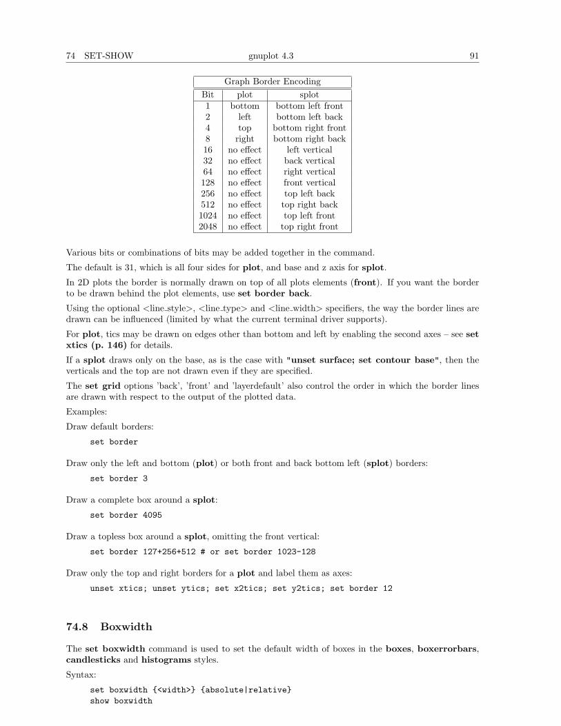
74 SET-SHOW gnuplot 4.3 91
Graph Border EncodingBit plot splot1 bottom bottom left front2 left bottom left back4 top bottom right front8 right bottom right back16 no effect left vertical32 no effect back vertical64 no effect right vertical128 no effect front vertical256 no effect top left back512 no effect top right back1024 no effect top left front2048 no effect top right front
Various bits or combinations of bits may be added together in the command.
The default is 31, which is all four sides for plot, and base and z axis for splot.
In 2D plots the border is normally drawn on top of all plots elements (front). If you want the borderto be drawn behind the plot elements, use set border back.
Using the optional <line style>, <line type> and <line width> specifiers, the way the border lines aredrawn can be influenced (limited by what the current terminal driver supports).
For plot, tics may be drawn on edges other than bottom and left by enabling the second axes – see setxtics (p. 146) for details.
If a splot draws only on the base, as is the case with "unset surface; set contour base", then theverticals and the top are not drawn even if they are specified.
The set grid options ’back’, ’front’ and ’layerdefault’ also control the order in which the border linesare drawn with respect to the output of the plotted data.
Examples:
Draw default borders:
set border
Draw only the left and bottom (plot) or both front and back bottom left (splot) borders:
set border 3
Draw a complete box around a splot:
set border 4095
Draw a topless box around a splot, omitting the front vertical:
set border 127+256+512 # or set border 1023-128
Draw only the top and right borders for a plot and label them as axes:
unset xtics; unset ytics; set x2tics; set y2tics; set border 12
74.8 Boxwidth
The set boxwidth command is used to set the default width of boxes in the boxes, boxerrorbars,candlesticks and histograms styles.
Syntax:
set boxwidth {<width>} {absolute|relative}show boxwidth
92 gnuplot 4.3 74 SET-SHOW
By default, adjacent boxes are extended in width until they touch each other. A different default widthmay be specified using the set boxwidth command. Relative widths are interpreted as being a fractionof this default width.
An explicit value for the boxwidth is interpreted as being a number of units along the current x axis(absolute) unless the modifier relative is given. If the x axis is a log-scale (see set log (p. 113)) thenthe value of boxwidth is truly "absolute" only at x=1; this physical width is maintained everywherealong the axis (i.e. the boxes do not become narrower the value of x increases). If the range spannedby a log scale x axis is far from x=1, some experimentation may be required to find a useful value ofboxwidth.
The default is superseded by explicit width information taken from an extra data column in styles boxesor boxerrorbars. In a four-column data set, the fourth column will be interpreted as the box widthunless the width is set to -2.0, in which case the width will be calculated automatically. See style boxes(p. 39) and style boxerrorbars (p. 38) for more details.
To set the box width to automatic use the command
set boxwidth
or, for four-column data,
set boxwidth -2
The same effect can be achieved with the using keyword in plot:
plot ’file’ using 1:2:3:4:(-2)
To set the box width to half of the automatic size use
set boxwidth 0.5 relative
To set the box width to an absolute value of 2 use
set boxwidth 2 absolute
74.9 Clabel
gnuplot will vary the linetype used for each contour level when clabel is set. When this option on (thedefault), a legend labels each linestyle with the z level it represents. It is not possible at present toseparate the contour labels from the surface key.
Syntax:
set clabel {’<format>’}unset clabelshow clabel
The default for the format string is %8.3g, which gives three decimal places. This may produce poorlabel alignment if the key is altered from its default configuration.
The first contour linetype, or only contour linetype when clabel is off, is the surface linetype +1; contourpoints are the same style as surface points.
See also set contour (p. 95).
74.10 Clip
gnuplot can clip data points and lines that are near the boundaries of a graph.
Syntax:
set clip <clip-type>unset clip <clip-type>show clip
74 SET-SHOW gnuplot 4.3 93
Three clip types for points and lines are supported by gnuplot: points, one, and two. One, two, or allthree clip types may be active for a single graph. Note that clipping of color filled quadrangles drawn bypm3d maps and surfaces is not controlled by this command, but by set pm3d clip1in and set pm3dclip4in.
The points clip type forces gnuplot to clip (actually, not plot at all) data points that fall within buttoo close to the boundaries. This is done so that large symbols used for points will not extend outsidethe boundary lines. Without clipping points near the boundaries, the plot may look bad. Adjusting thex and y ranges may give similar results.
Setting the one clip type causes gnuplot to draw a line segment which has only one of its two endpointswithin the graph. Only the in-range portion of the line is drawn. The alternative is to not draw anyportion of the line segment.
Some lines may have both endpoints out of range, but pass through the graph. Setting the two clip-typeallows the visible portion of these lines to be drawn.
In no case is a line drawn outside the graph.
The defaults are noclip points, clip one, and noclip two.
To check the state of all forms of clipping, useshow clip
For backward compatibility with older versions, the following forms are also permitted:set clipunset clip
set clip is synonymous with set clip points; unset clip turns off all three types of clipping.
74.11 Cntrparam
set cntrparam controls the generation of contours and their smoothness for a contour plot. showcontour displays current settings of cntrparam as well as contour.
Syntax:set cntrparam { { linear
| cubicspline| bspline| points <n>| order <n>| levels { auto {<n>} | <n>
| discrete <z1> {,<z2>{,<z3>...}}| incremental <start>, <incr> {,<end>}
}}
}show contour
This command has two functions. First, it sets the values of z for which contour points are to bedetermined (by linear interpolation between data points or function isosamples.) Second, it controls theway contours are drawn between the points determined to be of equal z. <n> should be an integralconstant expression and <z1>, <z2> ... any constant expressions. The parameters are:
linear, cubicspline, bspline — Controls type of approximation or interpolation. If linear, thenstraight line segments connect points of equal z magnitude. If cubicspline, then piecewise-linear con-tours are interpolated between the same equal z points to form somewhat smoother contours, but whichmay undulate. If bspline, a guaranteed-smoother curve is drawn, which only approximates the positionof the points of equal-z.
points — Eventually all drawings are done with piecewise-linear strokes. This number controls thenumber of line segments used to approximate the bspline or cubicspline curve. Number of cubicsplineor bspline segments (strokes) = points * number of linear segments.
94 gnuplot 4.3 74 SET-SHOW
order — Order of the bspline approximation to be used. The bigger this order is, the smoother theresulting contour. (Of course, higher order bspline curves will move further away from the originalpiecewise linear data.) This option is relevant for bspline mode only. Allowed values are integers in therange from 2 (linear) to 10.
levels — Selection of contour levels, controlled by auto (default), discrete, incremental, and <n>,number of contour levels.
For auto, <n> specifies a nominal number of levels; the actual number will be adjusted to give simplelabels. If the surface is bounded by zmin and zmax, contours will be generated at integer multiples ofdz between zmin and zmax, where dz is 1, 2, or 5 times some power of ten (like the step between twotic marks).
For levels discrete, contours will be generated at z = <z1>, <z2> ... as specified; the number ofdiscrete levels sets the number of contour levels. In discrete mode, any set cntrparam levels <n>are ignored.
For incremental, contours are generated at values of z beginning at <start> and increasing by<increment>, until the number of contours is reached. <end> is used to determine the number ofcontour levels, which will be changed by any subsequent set cntrparam levels <n>. If the z axis islogarithmic, <increment> will be interpreted as a factor, just like in set ztics.
If the command set cntrparam is given without any arguments specified, the defaults are used: linear,5 points, order 4, 5 auto levels.
Examples:set cntrparam bsplineset cntrparam points 7set cntrparam order 10
To select levels automatically, 5 if the level increment criteria are met:set cntrparam levels auto 5
To specify discrete levels at .1, .37, and .9:set cntrparam levels discrete .1,1/exp(1),.9
To specify levels from 0 to 4 with increment 1:set cntrparam levels incremental 0,1,4
To set the number of levels to 10 (changing an incremental end or possibly the number of auto levels):set cntrparam levels 10
To set the start and increment while retaining the number of levels:set cntrparam levels incremental 100,50
See also set contour (p. 95) for control of where the contours are drawn, and set clabel (p. 92) forcontrol of the format of the contour labels and linetypes.
See also
contours demo (contours.dem)
and
contours with user defined levels demo (discrete.dem).
74.12 Color box
The color scheme, i.e. the gradient of the smooth color with min z and max z values of pm3d’s palette,is drawn in a color box unless unset colorbox.
set colorboxset colorbox {
{ vertical | horizontal }
74 SET-SHOW gnuplot 4.3 95
{ default | user }{ origin x, y }{ size x, y }{ front | back }{ noborder | bdefault | border [line style] }
}show colorboxunset colorbox
Color box position can be default or user. If the latter is specified the values as given with the originand size subcommands are used. The box can be drawn after (front) or before (back) the graph or thesurface.
The orientation of the color gradient can be switched by options vertical and horizontal.
origin x, y and size x, y are used only in combination with the user option. The x and y values areinterpreted as screen coordinates by default, and this is the only legal option for 3D plots. 2D plots,including splot with set view map, allow any coordinate system to be specified. Try for example:
set colorbox horiz user origin .1,.02 size .8,.04
which will draw a horizontal gradient somewhere at the bottom of the graph.
border turns the border on (this is the default). noborder turns the border off. If an positive integerargument is given after border, it is used as a line style tag which is used for drawing the border, e.g.:
set style line 2604 linetype -1 linewidth .4set colorbox border 2604
will use line style 2604, a thin line with the default border color (-1) for drawing the border. bdefault(which is the default) will use the default border line style for drawing the border of the color box.
The axis of the color box is called cb and it is controlled by means of the usual axes commands,i.e. set/unset/show with cbrange, [m]cbtics, format cb, grid [m]cb, cblabel, and perhaps evencbdata, [no]cbdtics, [no]cbmtics.
set colorbox without any parameter switches the position to default. unset colorbox resets thedefault parameters for the colorbox and switches the colorbox off.
See also help for set pm3d (p. 123), set palette (p. 126), x11 pm3d (p. 209), and set style line(p. 136).
74.13 Colornames
Gnuplot knows a limited number of color names. You can use these to define the color range spannedby a pm3d palette, or to assign a terminal-independent color to a particular linetype or linestyle. To seethe list of known color names, use the command show colornames (p. 95). Example:
set style line 1 linecolor rgb "sea-green"
74.14 Contour
set contour enables contour drawing for surfaces. This option is available for splot only. It requiresgrid data, see grid data (p. 157) for more details. If contours are desired from non-grid data, setdgrid3d can be used to create an appropriate grid.
Syntax:set contour {base | surface | both}unset contourshow contour
The three options specify where to draw the contours: base draws the contours on the grid base wherethe x/ytics are placed, surface draws the contours on the surfaces themselves, and both draws thecontours on both the base and the surface. If no option is provided, the default is base.
96 gnuplot 4.3 74 SET-SHOW
See also set cntrparam (p. 93) for the parameters that affect the drawing of contours, and set clabel(p. 92) for control of labelling of the contours.
The surface can be switched off (see set surface (p. 137)), giving a contour-only graph. Though it ispossible to use set size to enlarge the plot to fill the screen, more control over the output format canbe obtained by writing the contour information to a file, and rereading it as a 2D datafile plot:
unset surfaceset contourset cntrparam ...set table ’filename’splot ...unset table# contour info now in filenameset term <whatever>plot ’filename’
In order to draw contours, the data should be organized as "grid data". In such a file all the points fora single y-isoline are listed, then all the points for the next y-isoline, and so on. A single blank line (aline containing no characters other than blank spaces and a carriage return and/or a line feed) separatesone y-isoline from the next. See also splot datafile (p. 154).
See also
contours demo (contours.dem)
and
contours with user defined levels demo (discrete.dem).
74.15 Data style
This form of the command is deprecated. Please see set style data (p. 134).
74.16 Datafile
The set datafile command options control interpretation of fields read from input data files by theplot, splot, and fit commands. Six such options are currently implemented.
74.16.1 Set datafile fortran
The set datafile fortran command enables a special check for values in the input file expressed asFortran D or Q constants. This extra check slows down the input process, and should only be selectedif you do in fact have datafiles containing Fortran D or Q constants. The option can be disabled againusing unset datafile fortran.
74.16.2 Set datafile nofpe trap
The set datafile nofpe trap command tells gnuplot not to re-initialize a floating point exception han-dler before every expression evaluation used while reading data from an input file. This can significantlyspeed data input from large files at the risk of program termination if a floating-point exception isgenerated.
74.16.3 Set datafile missing
The set datafile missing command allows you to tell gnuplot what character string is used in a datafile to denote missing data. Exactly how this missing value will be treated depends on the using specifierof the plot or splot command.
Syntax:
74 SET-SHOW gnuplot 4.3 97
set datafile missing {"<string>"}show datafile missingunset datafile
Example:# Ignore entries containing IEEE NaN ("Not a Number") codeset datafile missing "NaN"
Example:set datafile missing "?"set style data linesplot ’-’
1 102 203 ?4 405 50e
plot ’-’ using 1:21 102 203 ?4 405 50e
plot ’-’ using 1:($2)1 102 203 ?4 405 50e
The first plot will recognize only the first datum in the "3 ?" line. It will use the single-datum-on-a-lineconvention that the line number is "x" and the datum is "y", so the point will be plotted (in this caseerroneously) at (2,3).
The second plot will correctly ignore the middle line. The plotted line will connect the points at (2,20)and (4,40).
The third plot will also correctly ignore the middle line, but the plotted line will not connect the pointsat (2,20) and (4,40).
There is no default character for missing, but in many cases any non-parsible string of characters foundwhere a numerical value is expected will be treated as missing data.
74.16.4 Set datafile separator
The command set datafile separator "<char>" tells gnuplot that data fields in subsequent inputfiles are separated by <char> rather than by whitespace. The most common use is to read in csv(comma-separated value) files written by spreadsheet or database programs. By default data fields areseparated by whitespace.
Syntax:set datafile separator {"<char>" | whitespace}
Examples:# Input file contains tab-separated fieldsset datafile separator "\t"
# Input file contains comma-separated values fieldsset datafile separator ","

98 gnuplot 4.3 74 SET-SHOW
74.16.5 Set datafile commentschars
The set datafile commentschars command allows you to tell gnuplot what characters are used ina data file to denote comments. Gnuplot will ignore rest of the line behind the specified characters ifeither of them is the first non-blank character on the line.
Syntax:set datafile commentschars {"<string>"}show datafile commentscharsunset commentschars
Default value of the string is "#!" on VMS and "#" otherwise.
Then, the following line in a data file is completely ignored# 1 2 3 4
but the following1 # 3 4
produces rather unexpected plot unlessset datafile missing ’#’
is specified as well.
Example:set datafile commentschars "#!%"
74.16.6 Set datafile binary
The set datafile binary command is used to set the defaults when reading binary data files. Thesyntax matches precisely that used for commands plot and splot. See binary (p. 66) for details about<binary list>.
Syntax:set datafile binary <binary list>show datafile binaryshow datafileunset datafile
Examples:set datafile binary filetype=autoset datafile binary array=(512,512) format="%uchar"
show datafile binary # list current settings
74.17 Decimalsign
The set decimalsign command selects a decimal sign for numbers printed into tic labels or set labelstrings.
Syntax:set decimalsign {<value> | locale {"<locale>"}}unset decimalsignshow decimalsign
The argument <value> is a string to be used in place of the usual decimal point. Typical choices includethe period, ’.’, and the comma, ’,’, but others may be useful, too. If you omit the <value> argument,the decimal separator is not modified from the usual default, which is a period. Unsetting decimalsignhas the same effect as omitting <value>.
Example:
Correct typesetting in most European countries requires:
74 SET-SHOW gnuplot 4.3 99
set decimalsign ’,’
Please note: If you set an explicit string, this affects only numbers that are printed using gnuplot’sgprintf() formatting routine, include axis tics. It does not affect the format expected for input data, andit does not affect numbers printed with the sprintf() formatting routine. To change the behavior of bothinput and output formatting, instead use the form
set decimalsign locale
This instructs the program to use both input and output formats in accordance with the current settingof the LC ALL, LC NUMERIC, or LANG environmental variables.
set decimalsign locale "foo"
This instructs the program to format all input and output in accordance with locale "foo", which mustbe installed. If locale "foo" is not found then an error message is printed and the decimal sign settingis unchanged. On linux systems you can get a list of the locales installed on your machine by typing"locale -a". A typical linux locale string is of the form "sl SI.UTF-8". A typical Windows locale stringis of the form "Slovenian Slovenia.1250" or "slovenian". Please note that interpretation of the localesettings is done by the C library at runtime. Older C libraries may offer only partial support for localesettings such as the thousands grouping separator character.
set decimalsign locale; set decimalsign "."
This sets all input and output to use whatever decimal sign is correct for the current locale, but over-ridesthis with an explicit ’.’ in numbers formatted using gnuplot’s internal gprintf() function.
74.18 Dgrid3d
The set dgrid3d command enables, and can set parameters for, non-grid to grid data mapping. Seesplot grid data (p. 157) for more details about the grid data structure.
Syntax:set dgrid3d {<rows>} {,{<cols>}}
{ splines |qnorm {<norm>} |gauss | cauchy | exp | box | hann {<dx>} {,{dy}} }
unset dgrid3dshow dgrid3d
By default dgrid3d is disabled. When enabled, 3D data read from a file are always treated as a scattereddata set. A grid with dimensions derived from a bounding box of the scattered data and size as specifiedby the row/col size parameters is created for plotting and contouring. The grid is equally spaced inx (rows) and in y (columns); the z values are computed as weighted averages or spline interpolationsof the scattered points’ z values. In other words, a regularly spaced grid is created and the a smoothapproximation to the raw data is evaluated for all grid points. Only this approximation is plotted, butnot the raw data.
The number of columns defaults to the number of rows, which defaults to 10.
Several algorithms are available to calculate the approximation from the raw data. Some of thesealgorithms can take additional parameters. These interpolations are such the closer the data point is toa grid point, the more effect it has on that grid point.
The splines algorithm calculates an interpolation based on "thin plate splines". It does not takeadditional paramaters.
The qnorm algorithm calculates a weighted average of the input data at each grid point. Each datapoint is weighted inversely by its distance from the grid point raised to the norm power. (Actually, theweights are given by the inverse of dx^norm + dy^norm, where dx and dy are the components of theseparation of the grid point from each data point. For some norms that are powers of two, specifically4, 8, and 16, the computation is optimized by using the Euclidean distance in the weight calculation,
100 gnuplot 4.3 74 SET-SHOW
(dx^2+dy^2)^norm/2. However, any non-negative integer can be used.) The power of the norm can bespecified as a single optional parameter. This algorithm is the default.
Finally, several smoothing kernels are available to calculate weighted averages: z = Sum i w(d i) * z i/ Sum i w(d i), where z i is the value of the i-th data point and d i is the distance between the currentgrid point and the location of the i-th data point. All kernels assign higher weights to data points thatare close to the current grid point and lower weights to data points further away.
The following kernels are available:
gauss : w(d) = exp(-d*d)cauchy : w(d) = 1/(1 + d*d)exp : w(d) = exp(-d)box : w(d) = 1 if d<1
= 0 otherwisehann : w(d) = 0.5*(1-cos(2*pi*d)) if d<1
w(d) = 0 otherwise
When using one of these five smoothing kernels, up to two additional parameter can be specified: dxand dy. These are used to rescale the coordinate differences when calculating the distance: d i = sqrt(((x-x i)/dx)**2 + ((y-y i)/dy)**2 ), where x,y are the coordinates of the current grid point and x i,y iare the coordinates of the i-th data point. The value of dy defaults to the value of dx, which defaults to1. The parameters dx and dy make it possible to control the radius over which data points contributeto a grid point IN THE UNITS OF THE DATA ITSELF.
A slightly different syntax is also supported for reasons of backwards compatibility. If no interpolationalgorithm has been explicitly selected, the qnorm algorithm is assumed. Up to three comma-separated,optional paramaters can be specified, which are interpreted as the the number of rows, the number ofcolumns, and the norm value, respectively.
The dgrid3d option is a simple scheme which replaces scattered data with weighted averages on aregular grid.More sophisticated approaches to this problem exist and should be used to preprocess thedata outside gnuplot if this simple solution is found inadequate.
See also
dgrid3d.dem: dgrid3d demo.
and
scatter.dem: dgrid3d demo.
74.19 Dummy
The set dummy command changes the default dummy variable names.
Syntax:
set dummy {<dummy-var>} {,<dummy-var>}show dummy
By default, gnuplot assumes that the independent, or "dummy", variable for the plot command is"t" if in parametric or polar mode, or "x" otherwise. Similarly the independent variables for the splotcommand are "u" and "v" in parametric mode (splot cannot be used in polar mode), or "x" and "y"otherwise.
It may be more convenient to call a dummy variable by a more physically meaningful or conventionalname. For example, when plotting time functions:
set dummy tplot sin(t), cos(t)
At least one dummy variable must be set on the command; set dummy by itself will generate an errormessage.
Examples:

74 SET-SHOW gnuplot 4.3 101
set dummy u,vset dummy ,s
The second example sets the second variable to s.
74.20 Encoding
The set encoding command selects a character encoding. Syntax:
set encoding {<value>}set encoding localeshow encoding
Valid values are
default - tells a terminal to use its default encodingiso_8859_1 - the most common Western European encoding used by many
Unix workstations and by MS-Windows. This encoding isknown in the PostScript world as ’ISO-Latin1’.
iso_8859_15 - a variant of iso_8859_1 that includes the Euro symboliso_8859_2 - used in Central and Eastern Europeiso_8859_9 - used in Turkey (also known as Latin5)koi8r - popular Unix cyrillic encodingkoi8u - ukrainian Unix cyrillic encodingcp437 - codepage for MS-DOScp850 - codepage for OS/2, Western Europecp852 - codepage for OS/2, Central and Eastern Europecp1250 - codepage for MS Windows, Central and Eastern Europecp1254 - codepage for MS Windows, Turkish (superset of Latin5)utf8 - variable-length (multibyte) representation of Unicode
entry point for each character
The command set encoding locale is different from the other options. It attempts to determine thecurrent locale from the runtime environment. On most systems this is controlled by the environmentalvariables LC ALL, LC CTYPE, or LANG. This mechanism is necessary, for example, to pass multibytecharacter encodings such as UTF-8 or EUC JP to the wxt and cairopdf terminals. This command doesnot affect the locale-specific representation of dates or numbers. See also set locale (p. 113) and setdecimalsign (p. 98).
Generally you must set the encoding before setting the terminal type. Note that encoding is not sup-ported by all terminal drivers and that the device must be able to produce the desired non-standardcharacters.
74.21 Fit
The fit setting defines where the fit command writes its output. If this option was built into your versionof gnuplot, it also controls whether parameter errors from the fit will be written into variables.
Syntax:
set fit {logfile {"<filename>"}} {{no}errorvariables}unset fitshow fit
The <filename> argument must be enclosed in single or double quotes.
If no filename is given or unset fit is used the log file is reset to its default value "fit.log" or the valueof the environmental variable FIT LOG.
If the given logfile name ends with a / or \, it is interpreted to be a directory name, and the actualfilename will be "fit.log" in that directory.
102 gnuplot 4.3 74 SET-SHOW
If the errorvariables option is turned on, the error of each fitted parameter computed by fit will becopied to a user-defined variable whose name is formed by appending " err" to the name of the parameteritself. This is useful mainly to put the parameter and its error onto a plot of the data and the fittedfunction, for reference, as in:
set fit errorvariablesfit f(x) ’datafile’ using 1:2 via a, bprint "error of a is:", a_errset label ’a=%6.2f’, a, ’+/- %6.2f’, a_errplot ’datafile’ using 1:2, f(x)
74.22 Fontpath
The fontpath setting defines additional locations for font files searched when including font files. Cur-rently only the postscript terminal supports fontpath. If a file cannot be found in the current directory,the directories in fontpath are tried. Further documentation concerning the supported file formats isincluded in the terminal postscript section of the documentation.
Syntax:set fontpath {"pathlist1" {"pathlist2"...}}show fontpath
Path names may be entered as single directory names, or as a list of path names separated by a platform-specific path separator, eg. colon (’:’) on Unix, semicolon (’;’) on DOS/Windows/OS/2/Amiga plat-forms. The show fontpath, save and save set commands replace the platform-specific separator witha space character (’ ’) for maximum portability. If a directory name ends with an exclamation mark (’ !’)also the subdirectories of this directory are searched for font files.
If the environmental variable GNUPLOT FONTPATH is set, its contents are appended to fontpath. Ifit is not set, a system dependent default value is used. It is set by testing several directories for existencewhen using the fontpath the first time. Thus, the first call of set fontpath, show fontpath, savefontpath, plot, or splot with embedded font files takes a little more time. If you want to save this timeyou may set the environmental variable GNUPLOT FONTPATH since probing is switched off, then.You can find out which is the default fontpath by using show fontpath.
However, show fontpath prints the contents of user defined fontpath and system fontpath separately.Also, the save and save set commands save only the user specified parts of fontpath, for portabilityreasons.
Many other terminal drivers access TrueType fonts via the gd library. For these drivers the font searchpath is controlled by the environmental variable GDFONTPATH.
74.23 Format
The format of the tic-mark labels can be set with the set format command or with the set tics formator individual set {axis}tics format commands.
Syntax:set format {<axes>} {"<format-string>"}set format {<axes>} {’<format-string>’}show format
where <axes> is either x, y, xy, x2, y2, z, cb or nothing (which applies the format to all axes). Thefollowing two commands are equivalent:
set format y "%.2f"set ytics format "%.2f"
The length of the string is restricted to 100 characters. The default format is "% g", but other formatssuch as "%.2f" or "%3.0em" are often desirable. The format "$%g$" is often desirable for LaTeX. If no
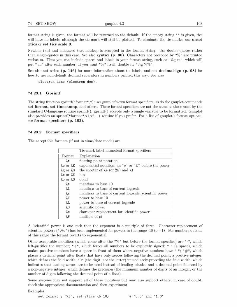
74 SET-SHOW gnuplot 4.3 103
format string is given, the format will be returned to the default. If the empty string "" is given, ticswill have no labels, although the tic mark will still be plotted. To eliminate the tic marks, use unsetxtics or set tics scale 0.
Newline (\n) and enhanced text markup is accepted in the format string. Use double-quotes ratherthan single-quotes in this case. See also syntax (p. 36). Characters not preceded by "%" are printedverbatim. Thus you can include spaces and labels in your format string, such as "%g m", which willput " m" after each number. If you want "%" itself, double it: "%g %%".
See also set xtics (p. 146) for more information about tic labels, and set decimalsign (p. 98) forhow to use non-default decimal separators in numbers printed this way. See also
electron demo (electron.dem).
74.23.1 Gprintf
The string function gprintf("format",x) uses gnuplot’s own format specifiers, as do the gnuplot commandsset format, set timestamp, and others. These format specifiers are not the same as those used by thestandard C-language routine sprintf(). gprintf() accepts only a single variable to be formatted. Gnuplotalso provides an sprintf("format",x1,x2,...) routine if you prefer. For a list of gnuplot’s format options,see format specifiers (p. 103).
74.23.2 Format specifiers
The acceptable formats (if not in time/date mode) are:
Tic-mark label numerical format specifiersFormat Explanation
%f floating point notation%e or %E exponential notation; an ”e” or ”E” before the power%g or %G the shorter of %e (or %E) and %f%x or %X hex%o or %O octal
%t mantissa to base 10%l mantissa to base of current logscale%s mantissa to base of current logscale; scientific power%T power to base 10%L power to base of current logscale%S scientific power%c character replacement for scientific power%P multiple of pi
A ’scientific’ power is one such that the exponent is a multiple of three. Character replacement ofscientific powers ("%c") has been implemented for powers in the range -18 to +18. For numbers outsideof this range the format reverts to exponential.
Other acceptable modifiers (which come after the "%" but before the format specifier) are "-", whichleft-justifies the number; "+", which forces all numbers to be explicitly signed; " " (a space), whichmakes positive numbers have a space in front of them where negative numbers have "-"; "#", whichplaces a decimal point after floats that have only zeroes following the decimal point; a positive integer,which defines the field width; "0" (the digit, not the letter) immediately preceding the field width, whichindicates that leading zeroes are to be used instead of leading blanks; and a decimal point followed bya non-negative integer, which defines the precision (the minimum number of digits of an integer, or thenumber of digits following the decimal point of a float).
Some systems may not support all of these modifiers but may also support others; in case of doubt,check the appropriate documentation and then experiment.
Examples:set format y "%t"; set ytics (5,10) # "5.0" and "1.0"
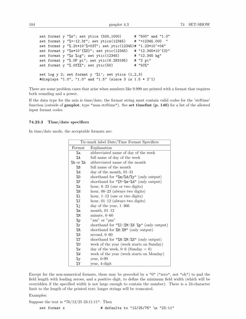
104 gnuplot 4.3 74 SET-SHOW
set format y "%s"; set ytics (500,1000) # "500" and "1.0"set format y "%+-12.3f"; set ytics(12345) # "+12345.000 "set format y "%.2t*10^%+03T"; set ytic(12345)# "1.23*10^+04"set format y "%s*10^{%S}"; set ytic(12345) # "12.345*10^{3}"set format y "%s %cg"; set ytic(12345) # "12.345 kg"set format y "%.0P pi"; set ytic(6.283185) # "2 pi"set format y "%.0f%%"; set ytic(50) # "50%"
set log y 2; set format y ’%l’; set ytics (1,2,3)#displays "1.0", "1.0" and "1.5" (since 3 is 1.5 * 2^1)
There are some problem cases that arise when numbers like 9.999 are printed with a format that requiresboth rounding and a power.
If the data type for the axis is time/date, the format string must contain valid codes for the ’strftime’function (outside of gnuplot, type "man strftime"). See set timefmt (p. 140) for a list of the allowedinput format codes.
74.23.3 Time/date specifiers
In time/date mode, the acceptable formats are:
Tic-mark label Date/Time Format SpecifiersFormat Explanation
%a abbreviated name of day of the week%A full name of day of the week
%b or %h abbreviated name of the month%B full name of the month%d day of the month, 01–31%D shorthand for "%m/%d/%y" (only output)%F shorthand for "%Y-%m-%d" (only output)%k hour, 0–23 (one or two digits)%H hour, 00–23 (always two digits)%l hour, 1–12 (one or two digits)%I hour, 01–12 (always two digits)%j day of the year, 1–366%m month, 01–12%M minute, 0–60%p ”am” or ”pm”%r shorthand for "%I:%M:%S %p" (only output)%R shorthand for %H:%M" (only output)%S second, 0–60%T shorthand for "%H:%M:%S" (only output)%U week of the year (week starts on Sunday)%w day of the week, 0–6 (Sunday = 0)%W week of the year (week starts on Monday)%y year, 0-99%Y year, 4-digit
Except for the non-numerical formats, these may be preceded by a "0" ("zero", not "oh") to pad thefield length with leading zeroes, and a positive digit, to define the minimum field width (which will beoverridden if the specified width is not large enough to contain the number). There is a 24-characterlimit to the length of the printed text; longer strings will be truncated.
Examples:
Suppose the text is "76/12/25 23:11:11". Thenset format x # defaults to "12/25/76" \n "23:11"
74 SET-SHOW gnuplot 4.3 105
set format x "%A, %d %b %Y" # "Saturday, 25 Dec 1976"set format x "%r %D" # "11:11:11 pm 12/25/76"
Suppose the text is "98/07/06 05:04:03". Thenset format x "%1y/%2m/%3d %01H:%02M:%03S" # "98/ 7/ 6 5:04:003"
74.24 Function style
This form of the command is deprecated. Please see set style function (p. 135).
74.25 Functions
The show functions command lists all user-defined functions and their definitions.
Syntax:show functions
For information about the definition and usage of functions in gnuplot, please see expressions (p. 23).See also
splines as user defined functions (spline.dem)
and
use of functions and complex variables for airfoils (airfoil.dem).
74.26 Grid
The set grid command allows grid lines to be drawn on the plot.
Syntax:set grid {{no}{m}xtics} {{no}{m}ytics} {{no}{m}ztics}
{{no}{m}x2tics} {{no}{m}y2tics}{{no}{m}cbtics}{polar {<angle>}}{layerdefault | front | back}{ {linestyle <major_linestyle>}| {linetype | lt <major_linetype>}{linewidth | lw <major_linewidth>}
{ , {linestyle | ls <minor_linestyle>}| {linetype | lt <minor_linetype>}{linewidth | lw <minor_linewidth>} } }
unset gridshow grid
The grid can be enabled and disabled for the major and/or minor tic marks on any axis, and the linetypeand linewidth can be specified for major and minor grid lines, also via a predefined linestyle, as far asthe active terminal driver supports this.
Additionally, a polar grid can be selected for 2D plots — circles are drawn to intersect the selected tics,and radial lines are drawn at definable intervals. (The interval is given in degrees or radians, dependingon the set angles setting.) Note that a polar grid is no longer automatically generated in polar mode.
The pertinent tics must be enabled before set grid can draw them; gnuplot will quietly ignore instruc-tions to draw grid lines at non-existent tics, but they will appear if the tics are subsequently enabled.
If no linetype is specified for the minor gridlines, the same linetype as the major gridlines is used. Thedefault polar angle is 30 degrees.
If front is given, the grid is drawn on top of the graphed data. If back is given, the grid is drawnunderneath the graphed data. Using front will prevent the grid from being obscured by dense data.
106 gnuplot 4.3 74 SET-SHOW
The default setup, layerdefault, is equivalent to back for 2d plots. In 3D plots the default is to splitup the grid and the graph box into two layers: one behind, the other in front of the plotted data andfunctions. Since hidden3d mode does its own sorting, it ignores all grid drawing order options andpasses the grid lines through the hidden line removal machinery instead. These options actually affectnot only the grid, but also the lines output by set border and the various ticmarks (see set xtics(p. 146)).
Z grid lines are drawn on the bottom of the plot. This looks better if a partial box is drawn around theplot — see set border (p. 90).
74.27 Hidden3d
The set hidden3d command enables hidden line removal for surface plotting (see splot (p. 153)).Some optional features of the underlying algorithm can also be controlled using this command.
Syntax:set hidden3d {defaults} |
{ {front|back}{{offset <offset>} | {nooffset}}{trianglepattern <bitpattern>}{{undefined <level>} | {noundefined}}{{no}altdiagonal}{{no}bentover} }
unset hidden3dshow hidden3d
In contrast to the usual display in gnuplot, hidden line removal actually treats the given function or datagrids as real surfaces that can’t be seen through, so plot elements behind the surface will be hidden byit. For this to work, the surface needs to have ’grid structure’ (see splot datafile (p. 154) about this),and it has to be drawn with lines or with linespoints.
When hidden3d is set, both the hidden portion of the surface and possibly its contours drawn on thebase (see set contour (p. 95)) as well as the grid will be hidden. Each surface has its hidden partsremoved with respect to itself and to other surfaces, if more than one surface is plotted. Contours drawnon the surface (set contour surface) don’t work.
Labels and arrows are always visible and are unaffected. The key box is never hidden by the surface.As of gnuplot version 4.2, set hidden3d also affects 3D plotting styles with points, with labels,and with vectors, even if no surface is present in the graph. Individual plots within the graph maybe explicitly excluded from this processing by appending the extra option nohidden3d to the withspecifier.
Hidden3d does not affect solid surfaces drawn using the pm3d mode. To achieve a similar effect purelyfor pm3d surfaces, use instead set pm3d depthorder. To mix pm3d surfaces with normal hidden3dprocessing, use the option set hidden3d front to force all elements included in hidden3d processing tobe drawn after any remaining plot elements. Then draw the surface twice, once with lines lt -2 anda second time with pm3d. The first instance will include the surface during calculation of occludedelements but will not draw the surface itself.
Functions are evaluated at isoline intersections. The algorithm interpolates linearly between functionpoints or data points when determining the visible line segments. This means that the appearance of afunction may be different when plotted with hidden3d than when plotted with nohidden3d becausein the latter case functions are evaluated at each sample. Please see set samples (p. 132) and setisosamples (p. 108) for discussion of the difference.
The algorithm used to remove the hidden parts of the surfaces has some additional features controllableby this command. Specifying defaults will set them all to their default settings, as detailed below.If defaults is not given, only explicitly specified options will be influenced: all others will keep theirprevious values, so you can turn on/off hidden line removal via set {no}hidden3d, without modifyingthe set of options you chose.
The first option, offset, influences the linestyle used for lines on the ’back’ side. Normally, they are
74 SET-SHOW gnuplot 4.3 107
drawn in a linestyle one index number higher than the one used for the front, to make the two sides ofthe surface distinguishable. You can specify a different line style offset to add instead of the default 1,by offset <offset>. Option nooffset stands for offset 0, making the two sides of the surface use thesame linestyle.
Next comes the option trianglepattern <bitpattern>. <bitpattern> must be a number between 0and 7, interpreted as a bit pattern. Each bit determines the visibility of one edge of the triangles eachsurface is split up into. Bit 0 is for the ’horizontal’ edges of the grid, Bit 1 for the ’vertical’ ones, andBit 2 for the diagonals that split each cell of the original grid into two triangles. The default pattern is3, making all horizontal and vertical lines visible, but not the diagonals. You may want to choose 7 tosee those diagonals as well.
The undefined <level> option lets you decide what the algorithm is to do with data points that areundefined (missing data, or undefined function values), or exceed the given x-, y- or z-ranges. Such pointscan either be plotted nevertheless, or taken out of the input data set. All surface elements touching apoint that is taken out will be taken out as well, thus creating a hole in the surface. If <level> = 3,equivalent to option noundefined, no points will be thrown away at all. This may produce all kinds ofproblems elsewhere, so you should avoid this. <level> = 2 will throw away undefined points, but keepthe out-of-range ones. <level> = 1, the default, will get rid of out-of-range points as well.
By specifying noaltdiagonal, you can override the default handling of a special case can occur ifundefined is active (i.e. <level> is not 3). Each cell of the grid-structured input surface will be dividedin two triangles along one of its diagonals. Normally, all these diagonals have the same orientation relativeto the grid. If exactly one of the four cell corners is excluded by the undefined handler, and this ison the usual diagonal, both triangles will be excluded. However if the default setting of altdiagonalis active, the other diagonal will be chosen for this cell instead, minimizing the size of the hole in thesurface.
The bentover option controls what happens to another special case, this time in conjunction with thetrianglepattern. For rather crumply surfaces, it can happen that the two triangles a surface cell isdivided into are seen from opposite sides (i.e. the original quadrangle is ’bent over’), as illustrated inthe following ASCII art:
C----Boriginal quadrangle: A--B displayed quadrangle: |\ |("set view 0,0") | /| ("set view 75,75" perhaps) | \ |
|/ | | \ |C--D | \|
A D
If the diagonal edges of the surface cells aren’t generally made visible by bit 2 of the <bitpattern> there,the edge CB above wouldn’t be drawn at all, normally, making the resulting display hard to understand.Therefore, the default option of bentover will turn it visible in this case. If you don’t want that, youmay choose nobentover instead. See also
hidden line removal demo (hidden.dem)
and
complex hidden line demo (singulr.dem).
74.28 Historysize
Note: the command set historysize is only available when gnuplot has been configured with the GNUreadline.
Syntax:set historysize <int>unset historysize
When leaving gnuplot, the value of historysize is used for truncating the history to at most that muchlines. The default is 500. unset historysize will disable history truncation and thus allow an infinitenumber of lines to be written to the history file.
108 gnuplot 4.3 74 SET-SHOW
74.29 Isosamples
The isoline density (grid) for plotting functions as surfaces may be changed by the set isosamplescommand.
Syntax:
set isosamples <iso_1> {,<iso_2>}show isosamples
Each function surface plot will have <iso 1> iso-u lines and <iso 2> iso-v lines. If you only specify<iso 1>, <iso 2> will be set to the same value as <iso 1>. By default, sampling is set to 10 isolinesper u or v axis. A higher sampling rate will produce more accurate plots, but will take longer. Theseparameters have no effect on data file plotting.
An isoline is a curve parameterized by one of the surface parameters while the other surface parameter isfixed. Isolines provide a simple means to display a surface. By fixing the u parameter of surface s(u,v),the iso-u lines of the form c(v) = s(u0,v) are produced, and by fixing the v parameter, the iso-v lines ofthe form c(u) = s(u,v0) are produced.
When a function surface plot is being done without the removal of hidden lines, set samples con-trols the number of points sampled along each isoline; see set samples (p. 132) and set hidden3d(p. 106). The contour algorithm assumes that a function sample occurs at each isoline intersection, sochange in samples as well as isosamples may be desired when changing the resolution of a functionsurface/contour.
74.30 Key
The set key command enables a key (or legend) describing plots on a plot.
The contents of the key, i.e., the names given to each plotted data set and function and samples ofthe lines and/or symbols used to represent them, are determined by the title and with options of the{s}plot command. Please see plot title (p. 80) and plot with (p. 80) for more information.
Syntax:
set key {on|off} {default}{{inside | outside} | {lmargin | rmargin | tmargin | bmargin}| {at <position>}}
{left | right | center} {top | bottom | center}{vertical | horizontal} {Left | Right}{{no}reverse} {{no}invert}{samplen <sample_length>} {spacing <vertical_spacing>}{width <width_increment>}{height <height_increment>}{{no}autotitle {columnheader}}{title "<text>"} {{no}enhanced}{font "<face>,<size>"} {textcolor <colorspec>}{{no}box { {linestyle | ls <line_style>}
| {linetype | lt <line_type>}{linewidth | lw <line_width>}}}
unset keyshow key
The key contains a title and a sample (line, point, box) for each plot in the graph. The key may beturned off by requesting set key off or unset key. Individual key entries may be turned off by usingthe notitle keyword in the corresponding plot command.
Elements within the key are stacked according to vertical or horizontal. In the case of vertical, thekey occupies as few columns as possible. That is, elements are aligned in a column until running out ofvertical space at which point a new column is started. In the case of horizontal, the key occupies asfew rows as possible.
74 SET-SHOW gnuplot 4.3 109
By default the key is placed in the upper right inside corner of the graph. The keywords left, right,top, bottom, center, inside, outside, lmargin, rmargin, tmargin, bmargin (, above, over,below and under) may be used to automatically place the key in other positions of the graph. Also anat <position> may be given to indicate precisely where the plot should be placed. In this case, thekeywords left, right, top, bottom and center serve an analogous purpose for alignment. For moreinformation, see key placement (p. 110).
Justification of the plot titles within the key is controlled by Left or Right (default). The text andsample can be reversed (reverse) and a box can be drawn around the key (box {...}) in a specifiedlinetype and linewidth, or a user-defined linestyle.
By default the first plot label is at the top of the key and successive labels are entered below it. Theinvert option causes the first label to be placed at the bottom of the key, with successive labels enteredabove it. This option is useful to force the vertical ordering of labels in the key to match the order ofbox types in a stacked histogram.
The <height increment> is a number of character heights to be added to or subtracted from the heightof the key box. This is useful mainly when you are putting a box around the key and want larger bordersaround the key entries.
All plotted curves of plots and splots are titled according to the default option autotitles. Theautomatic generation of titles can be suppressed by noautotitles; then only those titles explicitlydefined by (s)plot ... title ... will be drawn.
The set key autotitle columnheader command causes the first entry in each column of input datato be interpreted as a text string and used as a title for the corresponding plot. If the quantity beingplotted is a function of data from several columns, gnuplot may be confused as to which column to drawthe title from. In this case it is necessary to specify the column explicitly in the plot command, e.g.plot "datafile" using (($2+$3)/$4) title 3 with lines.
An overall title can be put on the key (title "<text>") — see also syntax (p. 36) for the distinctionbetween text in single- or double-quotes. The key title uses the same justification as do the plot titles.
The defaults for set key are on, right, top, vertical, Right, noreverse, noinvert, samplen 4,spacing 1.25, title "", and nobox. The default <linetype> is the same as that used for the plotborders. Entering set key default returns the key to its default configuration.
The key is drawn as a sequence of lines, with one plot described on each line. On the right-hand side(or the left-hand side, if reverse is selected) of each line is a representation that attempts to mimic theway the curve is plotted. On the other side of each line is the text description (the line title), obtainedfrom the plot command. The lines are vertically arranged so that an imaginary straight line divides theleft- and right-hand sides of the key. It is the coordinates of the top of this line that are specified withthe set key command. In a plot, only the x and y coordinates are used to specify the line position. Fora splot, x, y and z are all used as a 3D location mapped using the same mapping as the graph itself toform the required 2D screen position of the imaginary line.
When using the TeX or PostScript drivers, or similar drivers where formatting information is embeddedin the string, gnuplot is unable to calculate correctly the width of the string for key positioning. Ifthe key is to be positioned at the left, it may be convenient to use the combination set key left Leftreverse. The box and gap in the grid will be the width of the literal string.
If splot is being used to draw contours, the contour labels will be listed in the key. If the alignment ofthese labels is poor or a different number of decimal places is desired, the label format can be specified.See set clabel (p. 92) for details.
Examples:
This places the key at the default location:set key default
This disables the key:unset key
This places a key at coordinates 2,3.5,2 in the default (first) coordinate system:set key at 2,3.5,2
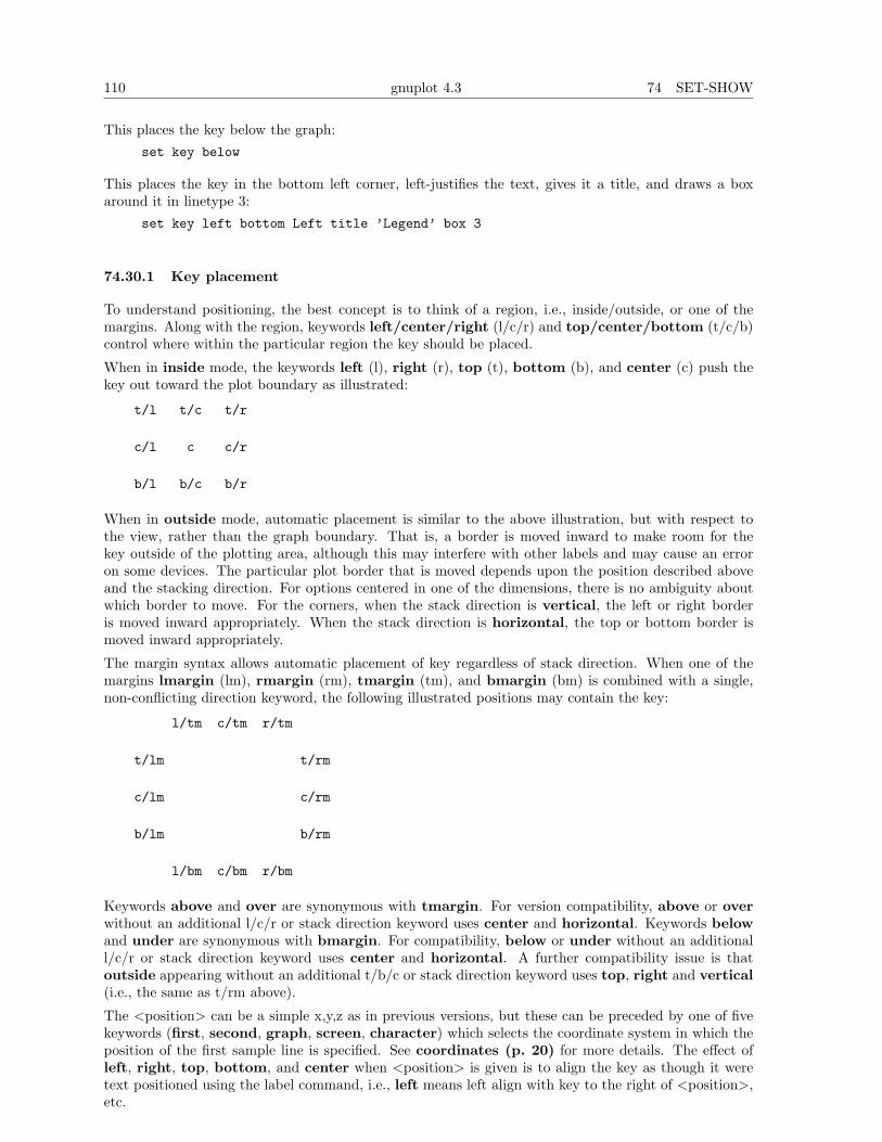
110 gnuplot 4.3 74 SET-SHOW
This places the key below the graph:set key below
This places the key in the bottom left corner, left-justifies the text, gives it a title, and draws a boxaround it in linetype 3:
set key left bottom Left title ’Legend’ box 3
74.30.1 Key placement
To understand positioning, the best concept is to think of a region, i.e., inside/outside, or one of themargins. Along with the region, keywords left/center/right (l/c/r) and top/center/bottom (t/c/b)control where within the particular region the key should be placed.
When in inside mode, the keywords left (l), right (r), top (t), bottom (b), and center (c) push thekey out toward the plot boundary as illustrated:
t/l t/c t/r
c/l c c/r
b/l b/c b/r
When in outside mode, automatic placement is similar to the above illustration, but with respect tothe view, rather than the graph boundary. That is, a border is moved inward to make room for thekey outside of the plotting area, although this may interfere with other labels and may cause an erroron some devices. The particular plot border that is moved depends upon the position described aboveand the stacking direction. For options centered in one of the dimensions, there is no ambiguity aboutwhich border to move. For the corners, when the stack direction is vertical, the left or right borderis moved inward appropriately. When the stack direction is horizontal, the top or bottom border ismoved inward appropriately.
The margin syntax allows automatic placement of key regardless of stack direction. When one of themargins lmargin (lm), rmargin (rm), tmargin (tm), and bmargin (bm) is combined with a single,non-conflicting direction keyword, the following illustrated positions may contain the key:
l/tm c/tm r/tm
t/lm t/rm
c/lm c/rm
b/lm b/rm
l/bm c/bm r/bm
Keywords above and over are synonymous with tmargin. For version compatibility, above or overwithout an additional l/c/r or stack direction keyword uses center and horizontal. Keywords belowand under are synonymous with bmargin. For compatibility, below or under without an additionall/c/r or stack direction keyword uses center and horizontal. A further compatibility issue is thatoutside appearing without an additional t/b/c or stack direction keyword uses top, right and vertical(i.e., the same as t/rm above).
The <position> can be a simple x,y,z as in previous versions, but these can be preceded by one of fivekeywords (first, second, graph, screen, character) which selects the coordinate system in which theposition of the first sample line is specified. See coordinates (p. 20) for more details. The effect ofleft, right, top, bottom, and center when <position> is given is to align the key as though it weretext positioned using the label command, i.e., left means left align with key to the right of <position>,etc.
74 SET-SHOW gnuplot 4.3 111
74.30.2 Key samples
By default, each plot on the graph generates a corresponding entry in the key. This entry contains aplot title and a sample line/point/box of the same color and fill properties as used in the plot itself. Thefont and textcolor properties control the appearance of the individual plot titles that appear in the key.Setting the textcolor to "rgb variable" causes the text for each key entry to be the same color as theline or fill color for that plot. This was the default in some earlier versions of gnuplot.
The length of the sample line can be controlled by samplen. The sample length is computed as the sumof the tic length and <sample length> times the character width. samplen also affects the positions ofpoint samples in the key since these are drawn at the midpoint of the sample line, even if the sampleline itself is not drawn.
The vertical spacing between lines is controlled by spacing. The spacing is set equal to the product ofthe pointsize, the vertical tic size, and <vertical spacing>. The program will guarantee that the verticalspacing is no smaller than the character height.
The <width increment> is a number of character widths to be added to or subtracted from the lengthof the string. This is useful only when you are putting a box around the key and you are using controlcharacters in the text. gnuplot simply counts the number of characters in the string when computingthe box width; this allows you to correct it.
74.31 Label
Arbitrary labels can be placed on the plot using the set label command.
Syntax:
set label {<tag>} {"<label text>"} {at <position>}{left | center | right}{norotate | rotate {by <degrees>}}{font "<name>{,<size>}"}{noenhanced}{front | back}{textcolor <colorspec>}{point <pointstyle> | nopoint}{offset <offset>}
unset label {<tag>}show label
The <position> is specified by either x,y or x,y,z, and may be preceded by first, second, graph,screen, or character to select the coordinate system. See coordinates (p. 20) for details.
The tag is an integer that is used to identify the label. If no <tag> is given, the lowest unused tagvalue is assigned automatically. The tag can be used to delete or modify a specific label. To changeany attribute of an existing label, use the set label command with the appropriate tag, and specify theparts of the label to be changed.
The <label text> can be a string constant, a string variable, or a string- valued expression. See strings(p. 34), sprintf (p. 25), and gprintf (p. 103).
By default, the text is placed flush left against the point x,y,z. To adjust the way the label is positionedwith respect to the point x,y,z, add the justification parameter, which may be left, right or center,indicating that the point is to be at the left, right or center of the text. Labels outside the plottedboundaries are permitted but may interfere with axis labels or other text.
If rotate is given, the label is written vertically (if the terminal can do so, of course). If rotateby <degrees> is given, conforming terminals will try to write the text at the specified angle; non-conforming terminals will treat this as vertical text.
Font and its size can be chosen explicitly by font "<name>{,<size>}" if the terminal supports fontsettings. Otherwise the default font of the terminal will be used.
Normally the enhanced text mode string interpretation, if enabled for the current terminal, is applied
112 gnuplot 4.3 74 SET-SHOW
to all text strings including label text. The noenhanced property can be used to exempt a specificlabel from the enhanced text mode processing. The can be useful if the label contains underscores, forexample. See enhanced text (p. 21).
If front is given, the label is written on top of the graphed data. If back is given (the default), the labelis written underneath the graphed data. Using front will prevent a label from being obscured by densedata.
textcolor <colorspec> changes the color of the label text. <colorspec> can be a linetype, an rgbcolor, or a palette mapping. See help for colorspec (p. 30) and palette (p. 126). textcolor may beabbreviated tc.‘tc default‘ resets the text color to its default state.‘tc lt <n>‘ sets the text color to that of line type <n>.‘tc ls <n>‘ sets the text color to that of line style <n>.‘tc palette z‘ selects a palette color corresponding to the label z position.‘tc palette cb <val>‘ selects a color corresponding to <val> on the colorbar.‘tc palette fraction <val>‘, with 0<=val<=1, selects a color corresponding to
the mapping [0:1] to grays/colors of the ‘palette‘.‘tc rgb "#RRGGBB"‘ selects an arbitrary 24-bit RGB color.
If a <pointstyle> is given, using keywords lt, pt and ps, see style (p. 80), a point with the given styleand color of the given line type is plotted at the label position and the text of the label is displacedslightly. This option is used by default for placing labels in mouse enhanced terminals. Use nopointto turn off the drawing of a point near the label (this is the default).
The displacement defaults to 1,1 in pointsize units if a <pointstyle> is given, 0,0 if no <pointstyle> isgiven. The displacement can be controlled by the optional offset <offset> where <offset> is specifiedby either x,y or x,y,z, and may be preceded by first, second, graph, screen, or character to selectthe coordinate system. See coordinates (p. 20) for details.
If one (or more) axis is timeseries, the appropriate coordinate should be given as a quoted time stringaccording to the timefmt format string. See set xdata (p. 143) and set timefmt (p. 140).
The EEPIC, Imagen, LaTeX, and TPIC drivers allow \\ in a string to specify a newline.
Label coordinates and text can also be read from a data file (see labels (p. 47)).
Examples:
To set a label at (1,2) to "y=x", use:set label "y=x" at 1,2
To set a Sigma of size 24, from the Symbol font set, at the center of the graph, use:set label "S" at graph 0.5,0.5 center font "Symbol,24"
To set a label "y=x^2" with the right of the text at (2,3,4), and tag the label as number 3, use:set label 3 "y=x^2" at 2,3,4 right
To change the preceding label to center justification, use:set label 3 center
To delete label number 2, use:unset label 2
To delete all labels, use:unset label
To show all labels (in tag order), use:show label
To set a label on a graph with a timeseries on the x axis, use, for example:set timefmt "%d/%m/%y,%H:%M"set label "Harvest" at "25/8/93",1
74 SET-SHOW gnuplot 4.3 113
To display a freshly fitted parameter on the plot with the data and the fitted function, do this after thefit, but before the plot:
set label sprintf("a = %3.5g",par_a) at 30,15bfit = gprintf("b = %s*10^%S",par_b)set label bfit at 30,20
To set a label displaced a little bit from a small point:set label ’origin’ at 0,0 point lt 1 pt 2 ps 3 offset 1,-1
To set a label whose color matches the z value (in this case 5.5) of some point on a 3D splot coloredusing pm3d:
set label ’text’ at 0,0,5.5 tc palette z
74.32 Lmargin
The command set lmargin sets the size of the left margin. Please see set margin (p. 115) for details.
74.33 Loadpath
The loadpath setting defines additional locations for data and command files searched by the call,load, plot and splot commands. If a file cannot be found in the current directory, the directories inloadpath are tried.
Syntax:set loadpath {"pathlist1" {"pathlist2"...}}show loadpath
Path names may be entered as single directory names, or as a list of path names separated by a platform-specific path separator, eg. colon (’:’) on Unix, semicolon (’;’) on DOS/Windows/OS/2/Amiga plat-forms. The show loadpath, save and save set commands replace the platform-specific separator witha space character (’ ’) for maximum portability.
If the environment variable GNUPLOT LIB is set, its contents are appended to loadpath. However,show loadpath prints the contents of user defined loadpath and system loadpath separately. Also, thesave and save set commands save only the user specified parts of loadpath, for portability reasons.
74.34 Locale
The locale setting determines the language with which {x,y,z}{d,m}tics will write the days andmonths.
Syntax:set locale {"<locale>"}
<locale> may be any language designation acceptable to your installation. See your system documen-tation for the available options. The command set locale "" will try to determine the locale from theLC TIME, LC ALL, or LANG environment variables.
To change the decimal point locale, see set decimalsign (p. 98). To change the character encoding tothe current locale, see set encoding (p. 101).
74.35 Logscale
Syntax:set logscale <axes> <base>unset logscale <axes>show logscale
114 gnuplot 4.3 74 SET-SHOW
where <axes> may be any combinations of x, x2, y, y2, z, and cb in any order, and where <base> isthe base of the log scaling. If <base> is not given, then 10 is assumed. If <axes> is not given, then allaxes are assumed. The command unset logscale turns off log scaling for the specified axes.
Examples:
To enable log scaling in both x and z axes:set logscale xz
To enable scaling log base 2 of the y axis:set logscale y 2
To enable z and color log axes for a pm3d plot:set logscale zcb
To disable z axis log scaling:unset logscale z
74.36 Macros
If command line macro substitution is enabled, then tokens in the command line of the form@<stringvariablename> will be replaced by the text string contained in <stringvariablename>. Seesubstitution (p. 35).
Syntax:set macros
74.37 Mapping
If data are provided to splot in spherical or cylindrical coordinates, the set mapping command shouldbe used to instruct gnuplot how to interpret them.
Syntax:set mapping {cartesian | spherical | cylindrical}
A cartesian coordinate system is used by default.
For a spherical coordinate system, the data occupy two or three columns (or using entries). The firsttwo are interpreted as the azimuthal and polar angles theta and phi (or "longitude" and "latitude"), inthe units specified by set angles. The radius r is taken from the third column if there is one, or is setto unity if there is no third column. The mapping is:
x = r * cos(theta) * cos(phi)y = r * sin(theta) * cos(phi)z = r * sin(phi)
Note that this is a "geographic" spherical system, rather than a "polar" one (that is, phi is measuredfrom the equator, rather than the pole).
For a cylindrical coordinate system, the data again occupy two or three columns. The first two areinterpreted as theta (in the units specified by set angles) and z. The radius is either taken from thethird column or set to unity, as in the spherical case. The mapping is:
x = r * cos(theta)y = r * sin(theta)z = z
The effects of mapping can be duplicated with the using filter on the splot command, but mappingmay be more convenient if many data files are to be processed. However even if mapping is used, usingmay still be necessary if the data in the file are not in the required order.
mapping has no effect on plot.
world.dem: mapping demos.
74 SET-SHOW gnuplot 4.3 115
74.38 Margin
The computed margins can be overridden by the set margin commands. show margin shows thecurrent settings.
Syntax:set bmargin {{at screen} <margin>}set lmargin {{at screen} <margin>}set rmargin {{at screen} <margin>}set tmargin {{at screen} <margin>}show margin
The default units of <margin> are character heights or widths, as appropriate. A positive value definesthe absolute size of the margin. A negative value (or none) causes gnuplot to revert to the computedvalue. For 3D plots, only the left margin can be set using character units.
The keywords at screen indicates that the margin is specified as a fraction of the full drawing area.This can be used to precisely line up the corners of individual 2D and 3D graphs in a multiplot. Thisplacement ignores the current values of set origin and set size, and is intended as an alternative methodfor positioning graphs within a multiplot.
Normally the margins of a plot are automatically calculated based on tics, tic labels, axis labels, the plottitle, the timestamp and the size of the key if it is outside the borders. If, however, tics are attachedto the axes (set xtics axis, for example), neither the tics themselves nor their labels will be includedin either the margin calculation or the calculation of the positions of other text to be written in themargin. This can lead to tic labels overwriting other text if the axis is very close to the border.
74.39 Mouse
The command set mouse enables mouse actions. Currently the pm, x11, ggi, windows and wxt terminalsare mouse enhanced. There are two mouse modes. The 2d-graph mode works for 2d graphs and for maps(i.e. splots with set view having z-rotation 0, 90, 180, 270 or 360 degrees, including set view map)and it allows tracing the position over graph, zooming, annotating graph etc. For 3d graphs splot, theview and scaling of the graph can be changed with mouse buttons 1 and 2. If additionally to thesebuttons the modifier <ctrl> is hold down, the coordinate system only is rotated which is useful for largedata sets. A vertical motion of Button 2 with the shift key hold down changes the ticslevel.
Mousing is not available in multiplot mode. When multiplot is finished using unset multiplot, thenthe mouse will be turned on again and acts on the last plot (like replot does).
Syntax:set mouse {doubleclick <ms>} {nodoubleclick} \
{{no}zoomcoordinates} \{noruler | ruler {at x,y}} \{polardistance{deg|tan} | nopolardistance} \{format <string>} \{clipboardformat <int>/<string>} \{mouseformat <int>/<string>} \{{no}labels {"labeloptions"}} \{{no}zoomjump} {{no}verbose}
unset mouse
The doubleclick resolution is given in milliseconds and used for Button 1 which copies the current mouseposition to the clipboard. If you want that to be done by single clicking a value of 0 ms can be used.The default value is 300 ms.
The option zoomcoordinates determines if the coordinates of the zoom box are drawn at the edgeswhile zooming. This is on by default.
The options noruler and ruler switch the ruler off and on, the latter optionally setting the origin at thegiven coordinates. While the ruler is on, the distance in user units from the ruler origin to the mouse isdisplayed continuously. By default, toggling the ruler has the key binding ’r’.
116 gnuplot 4.3 74 SET-SHOW
The option polardistance determines if the distance between the mouse cursor and the ruler is alsoshown in polar coordinates (distance and angle in degrees or tangent (slope)). This corresponds to thedefault key binding ’5’.
The format option takes a fprintf like format string which determines how floating point numbers areprinted to the drivers window and the clipboard. The default is "% #g".
clipboardformat and mouseformat are used for formatting the text on Button1 and Button2 ac-tions – copying the coordinates to the clipboard and temporarily annotating the mouse position. Thiscorresponds to the key bindings ’1’, ’2’, ’3’, ’4’ (see the driver’s documentation). If the argument is astring this string is used as c format specifier and should contain two float specifiers, e.g. set mousemouseformat "mouse = %5.2g, %10.2f". Use set mouse mouseformat "" to turn this string offagain.
The following formats are available (format 6 may only be selected if the format string was specifiedalready):
0 real coordinates in brackets e.g. [1.23, 2.45]1 real coordinates w/o brackets e.g. 1.23, 2.452 x == timefmt [(as set by ‘set timefmt‘), 2.45]3 x == date [31. 12. 1999, 2.45]4 x == time [23:59, 2.45]5 x == date / time [31. 12. 1999 23:59, 2.45]6 alt. format, specified as string ""
Choose the option labels to define persistent gnuplot labels using Button 2. The default is nolabels,which makes Button 2 draw only a temporary label at the mouse position. Labels are drawn with thecurrent setting of mouseformat. The labeloptions string is passed to the set label command. Thedefault is "point pointstyle 1" which will plot a small plus at the label position. Temporary labels willdisappear at the next replot or mouse zoom operation. Persistent labels can be removed by holding theCtrl-Key down while clicking Button 2 on the label’s point. The threshold for how close you must be tothe label is also determined by the pointsize.
If the option zoomjump is on, the mouse pointer will be automatically offset a small distance afterstarting a zoom region with button 3. This can be useful to avoid a tiny (or even empty) zoom region.zoomjump is off by default.
If the option verbose is turned on the communication commands are shown during execution. Thisoption can also be toggled by hitting 6 in the driver’s window. verbose is off by default.
Press ’h’ in the driver’s window for a short summary of the mouse and key bindings. This will alsodisplay user defined bindings or hotkeys which can be defined using the bind command, see help forbind (p. 31). Note, that user defined hotkeys may override the default bindings.
Press ’q’ in the driver’s window to close the window. This key cannot be overridden with the bindcommand.
See also help for bind (p. 31) and label (p. 111).
74.39.1 X11 mouse
If multiple X11 plot windows have been opened using the set term x11 <n> terminal option, thenonly the current plot window supports the entire range of mouse commands and hotkeys. The otherwindows will, however, continue to display mouse coordinates at the lower left.
For consistency with other screen terminals, X11 mouse support is turned on by default, wherever thestandard input comes from. However, on some UNIX flavors, special input devices as /dev/null mightnot be select-able; using such devices with the mouse turned on will hang gnuplot. Please turn offmousing with unset mouse if you are in this situation.
74 SET-SHOW gnuplot 4.3 117
74.40 Multiplot
The command set multiplot places gnuplot in the multiplot mode, in which several plots are placedon the same page, window, or screen.
Syntax:set multiplot { layout <rows>,<cols>
{rowsfirst|columnsfirst} {downwards|upwards}{title <page title>}{scale <xscale>{,<yscale>}} {offset <xoff>{,<yoff>}}
}unset multiplot
For some terminals, no plot is displayed until the command unset multiplot is given, which causes theentire page to be drawn and then returns gnuplot to its normal single-plot mode. For other terminals,each separate plot command produces an updated display, either by redrawing all previous ones andthe newly added plot, or by just adding the new plot to the existing display.
The area to be used by the next plot is not erased before doing the new plot. The clear command canbe used to do this if wanted, as is typically the case for "inset" plots.
Any labels or arrows that have been defined will be drawn for each plot according to the current sizeand origin (unless their coordinates are defined in the screen system). Just about everything else thatcan be set is applied to each plot, too. If you want something to appear only once on the page, forinstance a single time stamp, you’ll need to put a set time/unset time pair around one of the plot,splot or replot commands within the set multiplot/unset multiplot block.
The multiplot title is separate from the individual plot titles, if any. Space is reserved for it at the topof the page, spanning the full width of the canvas.
The commands set origin and set size must be used to correctly position each plot if no layout isspecified or if fine tuning is desired. See set origin (p. 121) and set size (p. 132) for details of theirusage.
Example:set multiplotset size 0.4,0.4set origin 0.1,0.1plot sin(x)set size 0.2,0.2set origin 0.5,0.5plot cos(x)unset multiplot
This displays a plot of cos(x) stacked above a plot of sin(x).
set size and set origin refer to the entire plotting area used for each plot. Please also see set termsize (p. 17). If you want to have the axes themselves line up, you can guarantee that the margins arethe same size with the set margin commands. See set margin (p. 115) for their use. Note that themargin settings are absolute, in character units, so the appearance of the graph in the remaining spacewill depend on the screen size of the display device, e.g., perhaps quite different on a video display anda printer.
With the layout option you can generate simple multiplots without having to give the set size and setorigin commands before each plot: Those are generated automatically, but can be overridden at anytime. With layout the display will be divided by a grid with <rows> rows and <cols> columns. Thisgrid is filled rows first or columns first depending on whether the corresponding option is given in themultiplot command. The stack of plots can grow downwards or upwards. Default is rowsfirst anddownwards.
Each plot can be scaled by scale and shifted with offset; if the y-values for scale or offset are omitted,the x-value will be used. unset multiplot will turn off the automatic layout and restore the values ofset size and set origin as they were before set multiplot layout.
Example:
118 gnuplot 4.3 74 SET-SHOW
set size 1,1set origin 0,0set multiplot layout 3,2 columnsfirst scale 1.1,0.9[ up to 6 plot commands here ]unset multiplot
The above example will produce 6 plots in 2 columns filled top to bottom, left to right. Each plot willhave a horizontal size of 1.1/2 and a vertical size of 0.9/3.
See also
multiplot demo (multiplt.dem)
74.41 Mx2tics
Minor tic marks along the x2 (top) axis are controlled by set mx2tics. Please see set mxtics (p. 118).
74.42 Mxtics
Minor tic marks along the x axis are controlled by set mxtics. They can be turned off with unsetmxtics. Similar commands control minor tics along the other axes.
Syntax:set mxtics {<freq> | default}unset mxticsshow mxtics
The same syntax applies to mytics, mztics, mx2tics, my2tics and mcbtics.
<freq> is the number of sub-intervals (NOT the number of minor tics) between major tics (the defaultfor a linear axis is either two or five depending on the major tics, so there are one or four minor ticsbetween major tics). Selecting default will return the number of minor ticks to its default value.
If the axis is logarithmic, the number of sub-intervals will be set to a reasonable number by default(based upon the length of a decade). This will be overridden if <freq> is given. However the usualminor tics (2, 3, ..., 8, 9 between 1 and 10, for example) are obtained by setting <freq> to 10, eventhough there are but nine sub-intervals.
To set minor tics at arbitrary positions, use the ("<label>" <pos> <level>, ...) form of set{x|x2|y|y2|z}tics with <label> empty and <level> set to 1.
The set m{x|x2|y|y2|z}tics commands work only when there are uniformly spaced major tics. If allmajor tics were placed explicitly by set {x|x2|y|y2|z}tics, then minor tic commands are ignored.Implicit major tics and explicit minor tics can be combined using set {x|x2|y|y2|z}tics and set{x|x2|y|y2|z}tics add.
Examples:set xtics 0, 5, 10set xtics add (7.5)set mxtics 5
Major tics at 0,5,7.5,10, minor tics at 1,2,3,4,6,7,8,9set logscale yset ytics format ""set ytics 1e-6, 10, 1set ytics add ("1" 1, ".1" 0.1, ".01" 0.01, "10^-3" 0.001, \
"10^-4" 0.0001)set mytics 10
Major tics with special formatting, minor tics at log positions
By default, minor tics are off for linear axes and on for logarithmic axes. They inherit the settings foraxis|border and {no}mirror specified for the major tics. Please see set xtics (p. 146) for informationabout these.
74 SET-SHOW gnuplot 4.3 119
74.43 My2tics
Minor tic marks along the y2 (right-hand) axis are controlled by set my2tics. Please see set mxtics(p. 118).
74.44 Mytics
Minor tic marks along the y axis are controlled by set mytics. Please see set mxtics (p. 118).
74.45 Mztics
Minor tic marks along the z axis are controlled by set mztics. Please see set mxtics (p. 118).
74.46 Object
The set object command defines a single object which will appear in all subsequent 2D plots. Youmay define as many objects as you like. Currently the supported object types are rectangle, circle,ellipse, and polygon. Rectangles inherit a default set of style properties (fill, color, border) from thoseset by the command set style rectangle, but each object can also be given individual style properties.Circles, ellipses, and polygons inherit the fill style from set style fill.
Syntax:set object <index>
<object-type> <object-properties>{front|back|behind} {fc|fillcolor <colorspec>} {fs <fillstyle>}{default} {lw|linewidth <width>}
<object-type> is either rectangle, ellipse, circle, or polygon. Each object type has its own set ofcharacteristic properties.
Setting front will draw the object in front of all plot elements, but behind any labels that are alsomarked front. Setting back will place the object behind all plot curves and labels. Setting behind willplace the object behind everything including the axes and back rectangles, thus
set object rectangle from screen 0,0 to screen 1,1 behind
can be used to provide a colored background for the entire graph or page.
The fill color of the object is taken from the <colorspec>. fillcolor may be abbreviated fc. The fillstyle is taken from <fillstyle>. See colorspec (p. 30) and fillstyle (p. 134). If the keyword defaultis given, these properties are inherited from the default settings at the time a plot is drawn. See setstyle rectangle (p. 137).
74.46.1 Rectangle
Syntax:set object <index> rectangle
{from <position> {to|rto} <position> |center <position> size <w>,<h> |at <position> size <w>,<h>}
The position of the rectangle may be specified by giving the position of two diagonal corners (bottomleft and top right) or by giving the position of the center followed by the width and the height. In eithercase the positions may be given in axis, graph, or screen coordinates. See coordinates (p. 20). Theoptions at and center are synonyms.
Examples:# Force the entire area enclosed by the axes to have background color cyanset object 1 rect from graph 0, graph 0 to graph 1, graph 1 backset object 1 rect fc rgb "cyan" fillstyle solid 1.0
120 gnuplot 4.3 74 SET-SHOW
# Position a red square with lower left at 0,0 and upper right at 2,3set object 2 rect from 0,0 to 2,3 fc lt 1
# Position an empty rectangle (no fill) with a blue borderset object 3 rect from 0,0 to 2,3 fs empty border rgb "blue"
# Return fill and color to the default style but leave vertices unchangedset object 2 rect default
74.46.2 Ellipse
Syntax:
set object <index> ellipse {at|center} <position> size <w>,<h>{angle <orientation>}{<other-object-properties>}
The position of the ellipse is specified by giving the center followed by the width and the height (actuallythe major and minor axes). The keywords at and center are synonyms. The center position may begiven in axis, graph, or screen coordinates. See coordinates (p. 20). The major and minor axis lengthsmust be given in axis coordinates. The orientation of the ellipse is specified by the angle between thehorizontal axis and the first axis of the ellipse. NB: If the x and y axis scales are not equal, then themajor/minor axis ratio will no longer be correct after rotation. This may be fixed in a later gnuplotversion.
Note that set object ellipse size <2r>,<2r> does not in general produce the same result as setobject circle <r>. The circle radius is always interpreted in terms of units along the x axis, and willalways produce a circle even if the x and y axis scales are different and even if the aspect ratio of yourplot is not 1. ’Set object ellipse’ interprets the first ’2r’ in terms of x axis units and the second ’2r’ interms of y axis units. This will only produce a circle if the x and y axis scales are identical and the plotaspect ratio is 1.
74.46.3 Circle
Syntax:
set object <index> circle {at|center} <position> size <radius>{arc [<begin>:<end>]}{<other-object-properties>}
The position of the circle is specified by giving the position of the center center followed by the radius.The keywords at and center are synonyms. The position and radius may be given in x-axis, graph,or canvas coordinates. See coordinates (p. 20). In all cases the radius is calculated relative to thehorizontal scale of the axis, graph, or canvas. Any disparity between the horizontal and vertical scalingwill be corrected for so that the result is always a circle.
By default a full circle is drawn. The optional qualifier arc specifies a starting angle and ending angle,in degrees, for one arc of the circle. The arc is always drawn counterclockwise.
74.46.4 Polygon
Syntax:
set object <index> polygonfrom <position> to <position> ... {to <position>}
or
from <position> rto <position> ... {rto <position>}
74 SET-SHOW gnuplot 4.3 121
The position of the polygon may be specified by giving the position of a sequence of vertices. These maybe given in axis, graph, or screen coordinates. If relative coordinates are used (rto) then the coordinatetype must match that of the previous vertex. See coordinates (p. 20).
Example:set object 1 polygon from 0,0 to 1,1 to 2,0set object 1 fc rgb "cyan" fillstyle solid 1.0 border lt -1
74.47 Offsets
Offsets provide a mechanism to put an empty boundary around the data inside an autoscaled graph.The offsets only affect the x1 and y1 axes, and only in 2D plot commands.
Syntax:set offsets <left>, <right>, <top>, <bottom>unset offsetsshow offsets
Each offset may be a constant or an expression. Each defaults to 0. By default, the left and right offsetsare given in units of the first x axis, the top and bottom offsets in units of the first y axis. Alternatively,you may specify the offsets as a fraction of the total axis range by using the keyword "graph". A positiveoffset expands the axis range in the specified direction, e.g., a positive bottom offset makes ymin morenegative. Negative offsets, while permitted, can have unexpected interactions with autoscaling andclipping. To prevent the auto-scaling from further adjusting your axis ranges, it is useful to also specify"set auto fix".
Example:set auto fixset offsets graph 0.05, 0, 2, 2plot sin(x)
This graph of sin(x) will have a y range [-3:3] because the function will be autoscaled to [-1:1] and thevertical offsets are each two. The x range will be [-11:10] because the default is [-10:10] and it has beenexpanded to the left by 0.05 of that total range.
74.48 Origin
The set origin command is used to specify the origin of a plotting surface (i.e., the graph and itsmargins) on the screen. The coordinates are given in the screen coordinate system (see coordinates(p. 20) for information about this system).
Syntax:set origin <x-origin>,<y-origin>
74.49 Output
By default, screens are displayed to the standard output. The set output command redirects thedisplay to the specified file or device.
Syntax:set output {"<filename>"}show output
The filename must be enclosed in quotes. If the filename is omitted, any output file opened by aprevious invocation of set output will be closed and new output will be sent to STDOUT. (If you givethe command set output "STDOUT", your output may be sent to a file named "STDOUT"! ["Maybe", not "will be", because some terminals, like x11 or wxt, ignore set output.])
122 gnuplot 4.3 74 SET-SHOW
When both set terminal and set output are used together, it is safest to give set terminal first,because some terminals set a flag which is needed in some operating systems. This would be the case,for example, if the operating system needs to know whether or not a file is to be formatted in order toopen it properly.
On machines with popen functions (Unix), output can be piped through a shell command if the firstnon-whitespace character of the filename is ’|’. For instance,
set output "|lpr -Plaser filename"set output "|lp -dlaser filename"
On MSDOS machines, set output "PRN" will direct the output to the default printer. On VMS,output can be sent directly to any spooled device. It is also possible to send the output to DECnettransparent tasks, which allows some flexibility.
74.50 Parametric
The set parametric command changes the meaning of plot (splot) from normal functions to para-metric functions. The command unset parametric restores the plotting style to normal, single-valuedexpression plotting.
Syntax:
set parametricunset parametricshow parametric
For 2D plotting, a parametric function is determined by a pair of parametric functions operating on aparameter. An example of a 2D parametric function would be plot sin(t),cos(t), which draws a circle(if the aspect ratio is set correctly — see set size (p. 132)). gnuplot will display an error message ifboth functions are not provided for a parametric plot.
For 3D plotting, the surface is described as x=f(u,v), y=g(u,v), z=h(u,v). Therefore a triplet of functionsis required. An example of a 3D parametric function would be cos(u)*cos(v),cos(u)*sin(v),sin(u),which draws a sphere. gnuplot will display an error message if all three functions are not provided fora parametric splot.
The total set of possible plots is a superset of the simple f(x) style plots, since the two functions candescribe the x and y values to be computed separately. In fact, plots of the type t,f(t) are equivalent tothose produced with f(x) because the x values are computed using the identity function. Similarly, 3Dplots of the type u,v,f(u,v) are equivalent to f(x,y).
Note that the order the parametric functions are specified is xfunction, yfunction (and zfunction) andthat each operates over the common parametric domain.
Also, the set parametric function implies a new range of values. Whereas the normal f(x) and f(x,y)style plotting assume an xrange and yrange (and zrange), the parametric mode additionally specifies atrange, urange, and vrange. These ranges may be set directly with set trange, set urange, and setvrange, or by specifying the range on the plot or splot commands. Currently the default range forthese parametric variables is [-5:5]. Setting the ranges to something more meaningful is expected.
74.51 Plot
The show plot command shows the current plotting command as it results from the last plot and/orsplot and possible subsequent replot commands.
In addition, the show plot add2history command adds this current plot command into the history.It is useful if you have used replot to add more curves to the current plot and you want to edit thewhole command now.
74 SET-SHOW gnuplot 4.3 123
74.52 Pm3d
pm3d is an splot style for drawing palette-mapped 3d and 4d data as color/gray maps and surfaces. Ituses a pm3d algorithm which allows plotting gridded as well as non-gridded data without preprocessing,even when the data scans do not have the same number of points.
Drawing of color surfaces is available on terminals supporting filled colored polygons with color mappingspecified by palette. Currently supported terminals includeScreen terminals:OS/2 Presentation ManagerX11Linux VGA (vgagl)GGIWindowsAquaTerm (Mac OS X)wxWidgets (wxt)
Files:PostScriptpslatex, pstex, epslatexgif, png, jpeg(x)figtgifcgmpdfsvgemf
Let us first describe how a map/surface is drawn. The input data come from an evaluated function orfrom an splot data file. Each surface consists of a sequence of separate scans (isolines). The pm3dalgorithm fills the region between two neighbouring points in one scan with another two points in thenext scan by a gray (or color) according to z-values (or according to an additional ’color’ column, seehelp for using (p. 74)) of these 4 corners; by default the 4 corner values are averaged, but this canbe changed by the option corners2color. In order to get a reasonable surface, the neighbouring scansshould not cross and the number of points in the neighbouring scans should not differ too much; ofcourse, the best plot is with scans having same number of points. There are no other requirements (e.g.the data need not be gridded). Another advantage is that the pm3d algorithm does not draw anythingoutside of the input (measured or calculated) region.
Surface coloring works with the following input data:
1. splot of function or of data file with one or three data columns: The gray/color scale is obtainedby mapping the averaged (or corners2color) z-coordinate of the four corners of the above-specifiedquadrangle into the range [min color z,max color z] of zrange or cbrange providing a gray value in therange [0:1]. This value can be used directly as the gray for gray maps. The normalized gray value canbe further mapped into a color — see set palette (p. 126) for the complete description.
2. splot of data file with two or four data columns: The gray/color value is obtained by using thelast-column coordinate instead of the z-value, thus allowing the color and the z-coordinate be mutuallyindependent. This can be used for 4d data drawing.
Other notes:
1. The term ’scan’ referenced above is used more among physicists than the term ’iso curve’ referencedin gnuplot documentation and sources. You measure maps recorded one scan after another scan, that’swhy.
2. The ’gray’ or ’color’ scale is a linear mapping of a continuous variable onto a smoothly varying paletteof colors. The mapping is shown in a rectangle next to the main plot. This documentation refers to thisas a "colorbox", and refers to the indexing variable as lying on the colorbox axis. See set colorbox(p. 94), set cbrange (p. 153).
3. To use pm3d coloring to generate a two-dimensional plot rather than a 3D surface, use set viewmap or set pm3d map.
124 gnuplot 4.3 74 SET-SHOW
Syntax (the options can be given in any order):set pm3d {
{ at <bst combination> }{ interpolate <steps in scan>,<steps between scans> }{ scansautomatic | scansforward | scansbackward | depthorder }{ flush { begin | center | end } }{ ftriangles | noftriangles }{ clip1in | clip4in }{ corners2color { mean|geomean|median|min|max|c1|c2|c3|c4 } }{ hidden3d <linestyle> | nohidden3d }{ implicit | explicit }{ map }
}show pm3dunset pm3d
Color surface is drawn if data or function style is set to pm3d globally or via ’with’ option, or if theoption implicit is on — then the pm3d surface is combined with the line surface mesh. See bottom ofthis section for mode details.
Color surface can be drawn at the base or top (then it is a gray/color planar map) or at z-coordinates ofsurface points (gray/color surface). This is defined by the at option with a string of up to 6 combinationsof b, t and s. For instance, at b plots at bottom only, at st plots firstly surface and then top map,while at bstbst will never by seriously used.
Colored quadrangles are plotted one after another. When plotting surfaces (at s), the later quadranglesoverlap (overdraw) the previous ones. (Gnuplot is not virtual reality tool to calculate intersections offilled polygon meshes.) You may try to switch between scansforward and scansbackward to forcethe first scan of the data to be plotted first or last. The default is scansautomatic where gnuplotmakes a guess about scans order. On the other hand, the depthorder option completely reorders thequadrangles. The rendering is performed after a depth sorting, which allows to visualize even complicatedsurfaces; see pm3d depthorder (p. 126) for more details.
If two subsequent scans do not have same number of points, then it has to be decided whether tostart taking points for quadrangles from the beginning of both scans (flush begin), from their ends(flush end) or to center them (flush center). Note, that flush (center|end) are incompatible withscansautomatic: if you specify flush center or flush end and scansautomatic is set, it is silentlyswitched to scansforward.
If two subsequent scans do not have the same number of points, the option ftriangles specifies whethercolor triangles are drawn at the scan tail(s) where there are not enough points in either of the scan. Thiscan be used to draw a smooth map boundary.
Clipping with respect to x, y coordinates of quadrangles can be done in two ways. clip1in: all 4 pointsof each quadrangle must be defined and at least 1 point of the quadrangle must lie in the x and y ranges.clip4in: all 4 points of each quadrangle must lie in the x and y ranges.
There is a single gray/color value associated to each drawn pm3d quadrangle (no smooth color changeamong vertices). The value is calculated from z-coordinates from the surrounding corners according tocorners2color <option>. The options ’mean’ (default), ’geomean’ and ’median’ produce various kindsof surface color smoothing, while options ’min’ and ’max’ choose minimal or maximal value, respectively.This may not be desired for pixel images or for maps with sharp and intense peaks, in which case theoptions ’c1’, ’c2’, ’c3’ or ’c4’ can be used instead to assign the quadrangle color based on the z-coordinateof only one corner. Some experimentation may be needed to determine which corner corresponds to ’c1’,as the orientation depends on the drawing direction. Because the pm3d algorithm does not extend thecolored surface outside the range of the input data points, the ’c<j>’ coloring options will result in pixelsalong two edges of the grid not contributing to the color of any quadrangle. For example, applying thepm3d algorithm to the 4x4 grid of data points in script demo/pm3d.dem (please have a look) producesonly (4-1)x(4-1)=9 colored rectangles.
Another drawing algorithm, which would draw quadrangles around a given node by taking corners fromaveraged (x,y)-coordinates of its surrounding 4 nodes while using node’s color, could be implemented in
74 SET-SHOW gnuplot 4.3 125
the future. This is already done for drawing images (2D grids) via image and rgbimage styles.
Notice that ranges of z-values and color-values for surfaces are adjustable independently by set zrange,set cbrange, as well as set log for z or cb. Maps can be adjusted by the cb-axis only; see also setview map (p. 142) and set colorbox (p. 94).
The option hidden3d takes as the argument a linestyle which must be created by set style line ....(The style need not to be present when setting pm3d, but it must be present when plotting). If set, linesare drawn using the specified line style, taking into account hidden line removal. This is by far moreefficient than using the command set hidden3d as it doesn’t really calculate hidden line removal, butjust draws the filled polygons in the correct order. So the recommended choice when using pm3d is
set pm3d at s hidden3d 100set style line 100 lt 5 lw 0.5unset hidden3dunset surfsplot x*x+y*y
There used to be an option {transparent|solid} to this command. Now you get the same effect from setgrid {front|layerdefault}, respectively.
The set pm3d map is an abbreviation for set pm3d at b; set view map; set style data pm3d;set style func pm3d;. It is used for backwards compatibility, when set view map was not available.Take care that you properly use zrange and cbrange for input data point filtering and color rangescaling, respectively; and also set (no)surface seems to have a (side?) effect.
The option interpolate will interpolate grid points into a finer mesh, and color each quadrangle appro-priately. For data files, this will smoothen the color surface, and enhance spikes in a color surface. Forfunctions, interpolation makes little sense, except to trade off precision for memory. It would usuallymake more sense to use samples and isosamples when working with functions.
The coloring setup as well as the color box drawing are determined by set palette. There can be onlyone palette for the current plot. Drawing of several surfaces with different palettes can be achieved bymultiplot with fixed origin and size; don’t forget to use set palette maxcolors when your terminalis running out of available colors.
On gnuplot start-up, mode is explicit. For historical and thus compatibility reasons, commands setpm3d; (i.e. no options) and set pm3d at X ... (i.e. at is the first option) sets mode implicit. Further,set pm3d; sets up the other options to their default.
If the option implicit is on, all surface plots will be plotted additionally to the default type, e.g.splot ’fred.dat’ with lines, ’lola.dat’ with lines
would give both plots (meshes) additionally to a pm3d surface. That’s what you are used to after setpm3d;.
If the option explicit is on (or implicit is off) only plots specified by the with pm3d attribute areplotted with a pm3d surface, e.g.:
splot ’fred.dat’ with lines, ’lola.dat’ with pm3d
would plot ’fred.dat’ with lines (and only lines) and ’lola.dat’ with a pm3d surface.
If you set the default data or function style to pm3d, e.g.:set style data pm3d
then the options implicit and explicit have no effect.
Note that when plotting several plots, they are plotted in the order given on the command line. This canbe of interest especially for filled surfaces which can overwrite and therefore hide part of earlier plots.
If with pm3d is specified in the splot command line, then it accepts the ’at’ option. The followingplots draw three color surfaces at different altitudes:
set border 4095set pm3d at ssplot 10*x with pm3d at b, x*x-y*y, x*x+y*y with pm3d at t
See also help for set palette (p. 126), set cbrange (p. 153), set colorbox (p. 94), x11 pm3d(p. 209) and definitely the demo file demo/pm3d.dem.
126 gnuplot 4.3 74 SET-SHOW
74.52.1 Depthorder
By default the quadrangles making up a pm3d solid surface are rendered in the order theyare encountered along the surface grid points. This order may be controlled by the optionsscansautomatic|scansforward|scansbackward. These scan options are not in general compatiblewith hidden-surface removal.
Gnuplot does not do true hidden surface removal for solid surfaces, but often it is sufficient to render thecomponent quadrangles in order from furthest to closest. This mode may be selected using the options
set pm3d depthorder hidden3d
The depthorder option orders the solid quadrangles; the hidden3d option similarly orders the bound-ing lines (if drawn). Note that the global option set hidden3d does not affect pm3d surfaces.
74.53 Palette
Palette is a color storage for use by pm3d, filled color contours or polygons, color histograms, colorgradient background, and whatever it is or it will be implemented... Here it stands for a palette ofsmooth "continuous" colors or grays, but let’s call it just a palette.
Color palettes require terminal entries for filled color polygons and palettes of smooth colors, are currentlyavailable for terminals listed in help for set pm3d. The range of color values are adjustable independentlyby set cbrange and set log cb. The whole color palette is visualized in the colorbox.
Syntax:set paletteset palette {
{ gray | color }{ gamma <gamma> }{ rgbformulae <r>,<g>,<b>| defined { ( <gray1> <color1> {, <grayN> <colorN>}... ) }| file ’<filename>’ {datafile-modifiers}| functions <R>,<G>,<B>
}{ model { RGB | HSV | CMY | YIQ | XYZ } }{ positive | negative }{ nops_allcF | ps_allcF }{ maxcolors <maxcolors> }
}show paletteshow palette palette <n> {{float | int}}show palette gradientshow palette fit2rgbformulaeshow palette rgbformulaeshow colornames
set palette (i.e. without options) sets up the default values. Otherwise, the options can be given inany order. show palette shows the current palette properties.
show palette gradient displays the gradient defining the palette (if appropriate). show palettergbformulae prints the available fixed gray –> color transformation formulae. show colornamesprints the known color names.
show palette palette <n> prints to the screen or to the file given by set print a table of RGBtriplets calculated for the current palette settings and a palette having <n> discrete colors. The defaultwide table can be limited to 3 columns of r,g,b float values [0..1] or integer values [0..255] by optionsfloat or int, respectively. This way, the current gnuplot color palette can be loaded into other imagingapplications, for example Octave. Additionally to this textual list of RGB table, you can use the testpalette command to plot the R,G,B profiles for the current palette.
The following options determine the coloring properties.
74 SET-SHOW gnuplot 4.3 127
Figure using this palette can be gray or color. For instance, in pm3d color surfaces the gray of eachsmall spot is obtained by mapping the averaged z-coordinate of the 4 corners of surface quadranglesinto the range [min z,max z] providing range of grays [0:1]. This value can be used directly as the grayfor gray maps. The color map requires a transformation gray –> (R,G,B), i.e. a mapping [0:1] –>([0:1],[0:1],[0:1]).
Basically two different types of mappings can be used: Analytic formulae to convert gray to color,or discrete mapping tables which are interpolated. palette rgbformulae and palette functionsuse analytic formulae whereas palette defined and palette file use interpolated tables. palettergbformulae reduces the size of postscript output to a minimum.
The command show palette fit2rgbformulae finds the best matching set palette rgbformulae forthe current set palette. Naturally, it makes sense to use it for non-rgbformulae palettes. This commandcan be found useful mainly for external programs using the same rgbformulae definition of palettes asgnuplot, like zimg (
http://zimg.sourceforge.net
).
set palette gray switches to a gray only palette. set palette rgbformulae, set palette defined,set palette file and set palette functions switch to a color mapping. set palette color is an easyway to switch back from the gray palette to the last color mapping.
Automatic gamma correction via set palette gamma <gamma> can be done for gray maps only (setpalette gray). Linear mapping to gray is for gamma equals 1, see test palette (p. 158). Gamma isignored for color mappings.
Most terminals support only discrete number of colors (e.g. 256 colors in gif). All entries of the paletteremaining after the default gnuplot linetype colors declaration are allocated for pm3d by default. Thenmultiplot could fail if there are no more color positions in the terminal available. Then you should useset palette maxcolors <maxcolors> with a reasonably small value. This option can also be used toseparate levels of z=constant in discrete steps, thus to emulate filled contours. Default value of 0 staysfor allocating all remaining entries in the terminal palette or for to use exact mapping to RGB.
RGB color space might not be the most useful color space to work in. For that reason you may changethe color space with model to one of RGB, HSV, CMY, YIQ and XYZ. Using color names for setpalette defined tables and a color space other than RGB will result in funny colors. All explanationhave been written for RGB color space, so please note, that R can be H, C, Y, or X, depending on theactual color space (G and B accordingly).
All values for all color spaces are limited to [0,1].
RGB stands for Red, Green and Blue; CMY stands for Cyan, Magenta and Yellow; HSV stands forHue, Saturation, and Value; YIQ is the color model used by the U.S. Commercial Color TelevisionBroadcasting, it is basically an RGB recoding with downward compatibility for black and white television;XYZ are the three primary colors of the color model defined by the ’Commission Internationale del’Eclairage’ (CIE). For more information on color models see:
http://en.wikipedia.org/wiki/Color space
74.53.1 Rgbformulae
For rgbformulae three suitable mapping functions have to be chosen. This is done via rgbformulae<r>,<g>,<b>. The available mapping functions are listed by show palette rgbformulae. Defaultis 7,5,15, some other examples are 3,11,6, 21,23,3 or 3,23,21. Negative numbers, like 3,-11,-6, meaninverted color (i.e. 1-gray passed into the formula, see also positive (p. 128) and negative (p. 128)options below).
Some nice schemes in RGB color space
7,5,15 ... traditional pm3d (black-blue-red-yellow)3,11,6 ... green-red-violet23,28,3 ... ocean (green-blue-white); try also all other permutations21,22,23 ... hot (black-red-yellow-white)
128 gnuplot 4.3 74 SET-SHOW
30,31,32 ... color printable on gray (black-blue-violet-yellow-white)33,13,10 ... rainbow (blue-green-yellow-red)34,35,36 ... AFM hot (black-red-yellow-white)
A full color palette in HSV color space3,2,2 ... red-yellow-green-cyan-blue-magenta-red
Please note that even if called rgbformulae the formulas might actually determine the <H>,<S>,<V>or <X>,<Y>,<Z> or ... color components as usual.
Use positive and negative to invert the figure colors.
Note that it is possible to find a set of the best matching rgbformulae for any other color scheme by thecommandshow palette fit2rgbformulae
74.53.2 Defined
Gray-to-rgb mapping can be manually set by use of palette defined: A color gradient is defined andused to give the rgb values. Such a gradient is a piecewise linear mapping from gray values in [0,1] tothe RGB space [0,1]x[0,1]x[0,1]. You have to specify the gray values and the corresponding RGB valuesin between a linear interpolation shall take place:
Syntax:set palette defined { ( <gray1> <color1> {, <grayN> <colorN>}... ) }
<grayX> are gray values which are mapped to [0,1] and <colorX> are the corresponding rgb colors.The color can be specified in three different ways:
<color> := { <r> <g> <b> | ’<color-name>’ | ’#rrggbb’ }
Either by three numbers (each in [0,1]) for red, green and blue, separated by whitespace, or the nameof the color in quotes or X style color specifiers also in quotes. You may freely mix the three types in agradient definition, but the named color "red" will be something strange if RGB is not selected as colorspace. Use show colornames for a list of known color names.
Please note, that even if written as <r>, this might actually be the <H> component in HSV color spaceor <X> in CIE-XYZ space, or ... depending on the selected color model.
The <gray> values have to form an ascending sequence of real numbers; the sequence will be automat-ically rescaled to [0,1].
set palette defined (without a gradient definition in braces) switches to RGB color space and uses apreset full-spectrum color gradient. Use show palette gradient to display the gradient.
Examples:
To produce a gray palette (useless but instructive) use:set palette model RGBset palette defined ( 0 "black", 1 "white" )
To produce a blue yellow red palette use (all equivalent):set palette defined ( 0 "blue", 1 "yellow", 2 "red" )set palette defined ( 0 0 0 1, 1 1 1 0, 2 1 0 0 )set palette defined ( 0 "#0000ff", 1 "#ffff00", 2 "#ff0000" )
To produce some rainbow-like palette use:set palette defined ( 0 "blue", 3 "green", 6 "yellow", 10 "red" )
Full color spectrum within HSV color space:set palette model HSVset palette defined ( 0 0 1 1, 1 1 1 1 )set palette defined ( 0 0 1 0, 1 0 1 1, 6 0.8333 1 1, 7 0.8333 0 1)
74 SET-SHOW gnuplot 4.3 129
To produce a palette with few colors only use:set palette model RGB maxcolors 4set palette defined ( 0 "blue", 1 "green", 2 "yellow", 3 "red" )
’Traffic light’ palette (non-smooth color jumps at gray = 1/3 and 2/3).set palette model RGBset palette defined (0 "dark-green", 1 "green", 1 "yellow", \
2 "dark-yellow", 2 "red", 3 "dark-red" )
74.53.3 Functions
Use set palette functions <Rexpr>, <Gexpr>, <Bexpr> to define three formulae for the R(gray),G(gray) and B(gray) mapping. The three formulae may depend on the variable gray which will takevalues in [0,1] and should also produce values in [0,1]. Please note that <Rexpr> might be a formulafor the H-value if HSV color space has been chosen (same for all other formulae and color spaces).
Examples:
To produce a full color palette use:set palette model HSV functions gray, 1, 1
A nice black to gold palette:set palette model XYZ functions gray**0.35, gray**0.5, gray**0.8
A gamma-corrected black and white palettegamma = 2.2color(gray) = gray**(1./gamma)set palette model RGB functions color(gray), color(gray), color(gray)
74.53.4 File
set palette file is basically a set palette defined (<gradient>) where <gradient> is read from adatafile. Either 4 columns (gray,R,G,B) or just three columns (R,G,B) have to be selected via the usingdata file modifier. In the three column case, the line number will be used as gray. The gray range isautomatically rescaled to [0,1]. The file is read as a normal data file, so all datafile modifiers can beused. Please note, that R might actually be e.g. H if HSV color space is selected.
As usual <filename> may be ’-’ which means that the data follow the command inline and are terminatedby a single e on a line of its own.
Use show palette gradient to display the gradient.
Examples:
Read in a palette of RGB triples each in range [0,255]:set palette file ’some-palette’ using ($1/255):($2/255):($3/255)
Equidistant rainbow (blue-green-yellow-red) palette:set palette model RGB file "-"0 0 10 1 01 1 01 0 0e
Binary palette files are supported as well, see binary general (p. 66). Example: put 64 triplets ofR,G,B doubles into file palette.bin and load it by
set palette file "palette.bin" binary record=64 using 1:2:3
130 gnuplot 4.3 74 SET-SHOW
74.53.5 Gamma correction
For gray mappings gamma correction can be turned on by set palette gamma <gamma>. <gamma>defaults to 1.5 which is quite suitable for most terminals.
For color mappings no automatic gamma correction is done by gnuplot. However, you may easilyimplement gamma correction. Here is an example for a gray scale image by use of explicit functions forthe red, green and blue component with slightly different values of gamma
Example:set palette model RGBset palette functions gray**0.64, gray**0.67, gray**0.70
To use gamma correction with interpolated gradients specify intermediate gray values with appropriatecolors. Instead of
set palette defined ( 0 0 0 0, 1 1 1 1 )
use e.g.set palette defined ( 0 0 0 0, 0.5 .73 .73 .73, 1 1 1 1 )
or even more intermediate points until the linear interpolation fits the "gamma corrected" interpolationwell enough.
74.53.6 Postscript
In order to reduce the size of postscript files, the gray value and not all three calculated r,g,b valuesare written to the file. Therefore the analytical formulae are coded directly in the postscript languageas a header just before the pm3d drawing, see /g and /cF definitions. Usually, it makes sense to writetherein definitions of only the 3 formulae used. But for multiplot or any other reason you may want tomanually edit the transformations directly in the postscript file. This is the default option nops allcF.Using the option ps allcF writes postscript definitions of all formulae. This you may find interesting ifyou want to edit the postscript file in order to have different palettes for different surfaces in one graph.Well, you can achieve this functionality by multiplot with fixed origin and size.
If pm3d map has been plotted from gridded or almost regular data with an output to a postscript file,then it is possible to reduce the size of this postscript file up to at about 50% by the enclosed awk scriptpm3dCompress.awk. This you may find interesting if you intend to keep the file for including it intoyour publication or before downloading a very large file into a slow printer. Usage:
awk -f pm3dCompress.awk thefile.ps >smallerfile.ps
If pm3d map has been plotted from rectangular gridded data with an output to a postscript file, then itis possible to reduce the file size even more by the enclosed awk script pm3dConvertToImage.awk.Usage:
awk -f pm3dConvertToImage.awk <thefile.ps >smallerfile.ps
You may manually change the postscript output from gray to color and vice versa and change thedefinition of <maxcolors>.
74.54 Pointsize
The set pointsize command scales the size of the points used in plots.
Syntax:set pointsize <multiplier>show pointsize
The default is a multiplier of 1.0. Larger pointsizes may be useful to make points more visible inbitmapped graphics.
The pointsize of a single plot may be changed on the plot command. See plot with (p. 80) for details.
Please note that the pointsize setting is not supported by all terminal types.
74 SET-SHOW gnuplot 4.3 131
74.55 Polar
The set polar command changes the meaning of the plot from rectangular coordinates to polar coordi-nates.
Syntax:
set polarunset polarshow polar
In polar coordinates, the dummy variable (t) is an angle. The default range of t is [0:2*pi], or, if degreeunits have been selected, to [0:360] (see set angles (p. 86)).
The command unset polar changes the meaning of the plot back to the default rectangular coordinatesystem.
The set polar command is not supported for splots. See the set mapping (p. 114) command forsimilar functionality for splot (p. 153)s.
While in polar coordinates the meaning of an expression in t is really r = f(t), where t is an angle ofrotation. The trange controls the domain (the angle) of the function, and the x and y ranges controlthe range of the graph in the x and y directions. Each of these ranges, as well as the rrange, may beautoscaled or set explicitly. Ffor details of all the ranges commands, see set xrange (p. 145).
Example:
set polarplot t*sin(t)plot [-2*pi:2*pi] [-3:3] [-3:3] t*sin(t)
The first plot uses the default polar angular domain of 0 to 2*pi. The radius and the size of the graphare scaled automatically. The second plot expands the domain, and restricts the size of the graph to[-3:3] in both directions.
You may want to set size square to have gnuplot try to make the aspect ratio equal to unity, so thatcircles look circular. See also
polar demos (polar.dem)
and
polar data plot (poldat.dem).
74.56 Print
The set print command redirects the output of the print command to a file.
Syntax:
set printset print "-"set print "<filename>"set print "<filename>" appendset print "|<shell_command>"
Without "<filename>", the output file is restored to <STDERR>. The <filename> "-" means<STDOUT>. The append flag causes the file to be opened in append mode. A <filename> startingwith "|" is opened as a pipe to the <shell command> on platforms that support piping.
74.57 Rmargin
The command set rmargin sets the size of the right margin. Please see set margin (p. 115) fordetails.
132 gnuplot 4.3 74 SET-SHOW
74.58 Rrange
The set rrange command sets the range of the radial coordinate for a graph in polar mode. Please seeset xrange (p. 145) for details.
74.59 Samples
The sampling rate of functions, or for interpolating data, may be changed by the set samples command.
Syntax:set samples <samples_1> {,<samples_2>}show samples
By default, sampling is set to 100 points. A higher sampling rate will produce more accurate plots,but will take longer. This parameter has no effect on data file plotting unless one of the interpola-tion/approximation options is used. See plot smooth (p. 71) re 2D data and set cntrparam (p. 93)and set dgrid3d (p. 99) re 3D data.
When a 2D graph is being done, only the value of <samples 1> is relevant.
When a surface plot is being done without the removal of hidden lines, the value of samples specifies thenumber of samples that are to be evaluated for the isolines. Each iso-v line will have <sample 1> samplesand each iso-u line will have <sample 2> samples. If you only specify <samples 1>, <samples 2> willbe set to the same value as <samples 1>. See also set isosamples (p. 108).
74.60 Size
Syntax:set size {{no}square | ratio <r> | noratio} {<xscale>,<yscale>}show size
The <xscale> and <yscale> values are scale factors for the size of the plot, which includes the graph,labels, and margins.
Important note:In earlier versions of gnuplot, some terminal types used the values from‘set size‘ to control also the size of the output canvas; others did not.In version 4.2 almost all terminals now follow the following convention:
set term <terminal type> size <XX>, <YY> controls the size of the output file, or canvas.Please see individual terminal documentation for allowed values of the size parameters. By default, theplot will fill this canvas.
set size <XX>, <YY> scales the plot itself relative to the size of the canvas. Scale values less than1 will cause the plot to not fill the entire canvas. Scale values larger than 1 will cause only a portion ofthe plot to fit on the canvas. Please be aware that setting scale values larger than 1 may cause problemson some terminal types.
ratio causes gnuplot to try to create a graph with an aspect ratio of <r> (the ratio of the y-axis lengthto the x-axis length) within the portion of the plot specified by <xscale> and <yscale>.
The meaning of a negative value for <r> is different. If <r>=-1, gnuplot tries to set the scales so thatthe unit has the same length on both the x and y axes (suitable for geographical data, for instance). If<r>=-2, the unit on y has twice the length of the unit on x, and so on.
The success of gnuplot in producing the requested aspect ratio depends on the terminal selected. Thegraph area will be the largest rectangle of aspect ratio <r> that will fit into the specified portion of theoutput (leaving adequate margins, of course).
square is a synonym for ratio 1.
Both noratio and nosquare return the graph to the default aspect ratio of the terminal, but do notreturn <xscale> or <yscale> to their default values (1.0).
74 SET-SHOW gnuplot 4.3 133
ratio and square have no effect on 3D plots, but do affect 3D projections created using set view map.See also set view equal (p. ??), which forces the x and y axes of a 3D onto the same scale.
Examples:
To set the size so that the plot fills the available canvas:
set size 1,1
To make the graph half size and square use:
set size square 0.5,0.5
To make the graph twice as high as wide use:
set size ratio 2
See also
airfoil demo.
74.61 Style
Default plotting styles are chosen with the set style data and set style function commands. See plotwith (p. 80) for information about how to override the default plotting style for individual functionsand data sets. See plotting styles (p. 38) for a complete list of styles.
Syntax:
set style function <style>set style data <style>show style functionshow style data
Default styles for specific plotting elements may also be set.
Syntax:
set style arrow <n> <arrowstyle>set style fill <fillstyle>set style histogram <histogram style options>set style line <n> <linestyle>
74.61.1 Set style arrow
Each terminal has a default set of arrow and point types, which can be seen by using the command test.set style arrow defines a set of arrow types and widths and point types and sizes so that you can referto them later by an index instead of repeating all the information at each invocation.
Syntax:
set style arrow <index> defaultset style arrow <index> {nohead | head | heads}
{size <length>,<angle>{,<backangle>}}{filled | empty | nofilled}{front | back}{ {linestyle | ls <line_style>}| {linetype | lt <line_type>}{linewidth | lw <line_width} }
unset style arrowshow style arrow
<index> is an integer that identifies the arrowstyle.
If default is given all arrow style parameters are set to their default values.
134 gnuplot 4.3 74 SET-SHOW
If the linestyle <index> already exists, only the given parameters are changed while all others arepreserved. If not, all undefined values are set to the default values.
Specifying nohead produces arrows drawn without a head — a line segment. This gives you yet anotherway to draw a line segment on the plot. By default, arrows have one head. Specifying heads drawsarrow heads on both ends of the line.
Head size can be controlled by size <length>,<angle> or size <length>,<angle>,<backangle>,where <length> defines length of each branch of the arrow head and <angle> the angle (in degrees)they make with the arrow. <Length> is in x-axis units; this can be changed by first, second, graph,screen, or character before the <length>; see coordinates (p. 20) for details. <Backangle> onlytakes effect when filled or empty is also used. Then, <backangle> is the angle (in degrees) the backbranches make with the arrow (in the same direction as <angle>). The fig terminal has a restrictedbackangle function. It supports three different angles. There are two thresholds: Below 70 degrees, thearrow head gets an indented back angle. Above 110 degrees, the arrow head has an acute back angle.Between these thresholds, the back line is straight.
Specifying filled produces filled arrow heads (if heads are used). Filling is supported on filled-polygoncapable terminals, see help of pm3d (p. 123) for their list, otherwise the arrow heads are closed butnot filled. The same result (closed but not filled arrow head) is reached by specifying empty. Further,filling and outline is obviously not supported on terminals drawing arrows by their own specific routines,like metafont, metapost, latex or tgif.
The line style may be selected from a user-defined list of line styles (see set style line (p. 136)) or maybe defined here by providing values for <line type> (an index from the default list of styles) and/or<line width> (which is a multiplier for the default width).
Note, however, that if a user-defined line style has been selected, its properties (type and width) cannotbe altered merely by issuing another set style arrow command with the appropriate index and lt orlw.
If front is given, the arrows are written on top of the graphed data. If back is given (the default), thearrow is written underneath the graphed data. Using front will prevent a arrow from being obscuredby dense data.
Examples:
To draw an arrow without an arrow head and double width, use:set style arrow 1 nohead lw 2set arrow arrowstyle 1
See also set arrow (p. 86) for further examples.
74.61.2 Set style data
The set style data command changes the default plotting style for data plots.
Syntax:set style data <plotting-style>show style data
See plotting styles (p. 38) for the choices. If no choice is given, the choices are listed. show styledata shows the current default data plotting style.
74.61.3 Set style fill
The set style fill command is used to set the default style of the plot elements in plots with boxes, his-tograms, candlesticks and filledcurves. This default can be superseded by fillstyles attached to individualplots. See also ’set style rectangle’.
Syntax:set style fill {empty
| {transparent} solid {<density>}
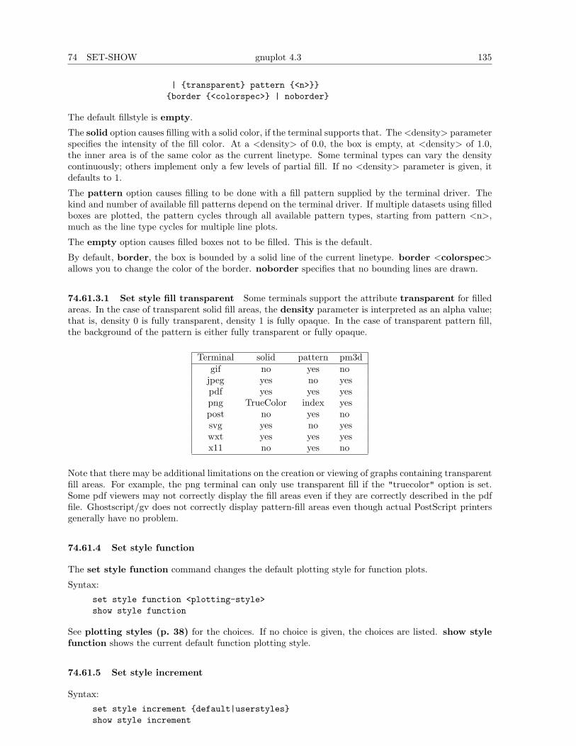
74 SET-SHOW gnuplot 4.3 135
| {transparent} pattern {<n>}}{border {<colorspec>} | noborder}
The default fillstyle is empty.
The solid option causes filling with a solid color, if the terminal supports that. The <density> parameterspecifies the intensity of the fill color. At a <density> of 0.0, the box is empty, at <density> of 1.0,the inner area is of the same color as the current linetype. Some terminal types can vary the densitycontinuously; others implement only a few levels of partial fill. If no <density> parameter is given, itdefaults to 1.
The pattern option causes filling to be done with a fill pattern supplied by the terminal driver. Thekind and number of available fill patterns depend on the terminal driver. If multiple datasets using filledboxes are plotted, the pattern cycles through all available pattern types, starting from pattern <n>,much as the line type cycles for multiple line plots.
The empty option causes filled boxes not to be filled. This is the default.
By default, border, the box is bounded by a solid line of the current linetype. border <colorspec>allows you to change the color of the border. noborder specifies that no bounding lines are drawn.
74.61.3.1 Set style fill transparent Some terminals support the attribute transparent for filledareas. In the case of transparent solid fill areas, the density parameter is interpreted as an alpha value;that is, density 0 is fully transparent, density 1 is fully opaque. In the case of transparent pattern fill,the background of the pattern is either fully transparent or fully opaque.
Terminal solid pattern pm3dgif no yes no
jpeg yes no yespdf yes yes yespng TrueColor index yespost no yes nosvg yes no yeswxt yes yes yesx11 no yes no
Note that there may be additional limitations on the creation or viewing of graphs containing transparentfill areas. For example, the png terminal can only use transparent fill if the "truecolor" option is set.Some pdf viewers may not correctly display the fill areas even if they are correctly described in the pdffile. Ghostscript/gv does not correctly display pattern-fill areas even though actual PostScript printersgenerally have no problem.
74.61.4 Set style function
The set style function command changes the default plotting style for function plots.
Syntax:
set style function <plotting-style>show style function
See plotting styles (p. 38) for the choices. If no choice is given, the choices are listed. show stylefunction shows the current default function plotting style.
74.61.5 Set style increment
Syntax:
set style increment {default|userstyles}show style increment
136 gnuplot 4.3 74 SET-SHOW
By default, successive plots within the same graph will use successive linetypes from the default set forthe current terminal type. However, choosing set style increment user allows you to step throughthe user-defined line styles rather than through the default linetypes.
Example:set style line 1 lw 2 lc rgb "gold"set style line 2 lw 2 lc rgb "purple"set style line 4 lw 1 lc rgb "sea-green"set style increment user
plot f1(x), f2(x), f3(x), f4(x)
should plot functions f1, f2, f4 in your 3 newly defined line styles. If a user-defined line style is not foundthen the corresponding default linetype is used instead. E.g. in the example above, f3(x) will be plottedusing the default linetype 3.
74.61.6 Set style line
Each terminal has a default set of line and point types, which can be seen by using the command test.set style line defines a set of line types and widths and point types and sizes so that you can refer tothem later by an index instead of repeating all the information at each invocation.
Syntax:set style line <index> defaultset style line <index> {{linetype | lt} <line_type> | <colorspec>}
{{linecolor | lc} <colorspec>}{{linewidth | lw} <line_width>}{{pointtype | pt} <point_type>}{{pointsize | ps} <point_size>}{palette}
unset style lineshow style line
If default is given all line style parameters are set to their default values.
If the linestyle <index> already exists, only the given parameters are changed while all others arepreserved. If not, all undefined values are set to the default values.
The line and point types are taken from the default types for the terminal currently in use. The linewidth and point size are multipliers for the default width and size (but note that <point size> here isunaffected by the multiplier given on set pointsize).
The defaults for the line and point types is the index. The defaults for the width and size are both unity.
Linestyles created by this mechanism do not replace the default linetype styles; both may be used. Ifyou want plots to use the defined styles in preference to the default linetypes, please see set styleincrement (p. 135).
Not all terminals support the linewidth and pointsize features; if not supported, the option will beignored.
Terminal-independent colors may be assigned using either linecolor <colorspec> or linetype<colorspec>, abbreviated lc or lt. This requires giving a RGB color triple, a known palette colorname, a fractional index into the current palette, or a constant value from the current mapping of thepalette onto cbrange. See colors (p. 29), colorspec (p. 30), set palette (p. 126), colornames(p. 95), cbrange (p. 153).
set style line <n> linetype <lt> will set both a terminal-dependent dot/dash pattern and color. Thecommandsset style line <n> linecolor <colorspec> or set style line <n> linetype <colorspec>will set a new line color while leaving the existing dot-dash pattern unchanged.
In 3d mode (splot command), the special keyword palette is allowed as a shorthand for "linetypepalette z". The color value corresponds to the z-value (elevation) of the splot, and varies smoothly alonga line or surface.
74 SET-SHOW gnuplot 4.3 137
Examples: Suppose that the default lines for indices 1, 2, and 3 are red, green, and blue, respectively,and the default point shapes for the same indices are a square, a cross, and a triangle, respectively. Then
set style line 1 lt 2 lw 2 pt 3 ps 0.5
defines a new linestyle that is green and twice the default width and a new pointstyle that is a half-sizedtriangle. The commands
set style function linesplot f(x) lt 3, g(x) ls 1
will create a plot of f(x) using the default blue line and a plot of g(x) using the user-defined wide greenline. Similarly the commands
set style function linespointsplot p(x) lt 1 pt 3, q(x) ls 1
will create a plot of p(x) using the default triangles connected by a red line and q(x) using small trianglesconnected by a green line.
splot sin(sqrt(x*x+y*y))/sqrt(x*x+y*y) w l pal
creates a surface plot using smooth colors according to palette. Note, that this works only on someterminals. See also set palette (p. 126), set pm3d (p. 123).
set style line 10 linetype 1 linecolor rgb "cyan"
will assign linestyle 10 to be a solid cyan line on any terminal that supports rgb colors.
74.61.7 Set style rectangle
Rectangles defined with the set object command can have individual styles. However, if the objectis not assigned a private style then it inherits a default that is taken from the set style rectanglecommand.
Syntax:set style rectangle {front|back} {lw|linewidth <lw>}
{fillcolor <colorspec>} {fs <fillstyle>}
See colorspec (p. 30) and fillstyle (p. 134). fillcolor may be abbreviated as fc.
Examples:set style rectangle back fc rgb "white" fs solid 1.0 border lt -1set style rectangle fc linsestyle 3 fs pattern 2 noborder
The default values correspond to solid fill with the background color and a black border.
74.62 Surface
The command set surface controls the display of surfaces by splot.
Syntax:set surfaceunset surfaceshow surface
The surface is drawn with the style specified by with, or else the appropriate style, data or function.
Whenever unset surface is issued, splot will not draw points or lines corresponding to the functionor data file points. Contours may still be drawn on the surface, depending on the set contour option.unset surface; set contour base is useful for displaying contours on the grid base. See also setcontour (p. 95).
138 gnuplot 4.3 74 SET-SHOW
74.63 Table
When table mode is enabled, plot and splot commands print out a multicolumn ASCII table of XY {Z} R values rather than creating an actual plot on the current terminal. The character R takeson one of three values: "i" if the point is in the active range, "o" if it is out-of-range, or "u" if it isundefined. The data format is determined by the format of the axis labels (see set format (p. 102)),and the columns are separated by single spaces. This can be useful if you want to generate contours andthen save them for further use, perhaps for plotting with plot; see set contour (p. 95) for example.The same method can be used to save interpolated data (see set samples (p. 132) and set dgrid3d(p. 99)).
Syntax:
set table {"outfile"}plot <whatever>unset table
Tabular output is written to the named file, if any, otherwise it is written to the current value of setoutput. You must explicitly unset table in order to go back to normal plotting on the current terminal.
74.64 Terminal
gnuplot supports many different graphics devices. Use set terminal to tell gnuplot what kind ofoutput to generate. Use set output to redirect that output to a file or device.
Syntax:
set terminal {<terminal-type> | push | pop}show terminal
If <terminal-type> is omitted, gnuplot will list the available terminal types. <terminal-type> may beabbreviated.
If both set terminal and set output are used together, it is safest to give set terminal first, becausesome terminals set a flag which is needed in some operating systems.
Several terminals have many additional options. For example, see png (p. 188), or postscript (p. 191).The options used by a previous invocation set term <term> <options> of a given <term> areremembered, thus subsequent set term <term> does not reset them. This helps in printing, forinstance, when switching among different terminals — previous options don’t have to be repeated.
The command set term push remembers the current terminal including its settings while set termpop restores it. This is equivalent to save term and load term, but without accessing the filesystem.Therefore they can be used to achieve platform independent restoring of the terminal after printing, forinstance. After gnuplot’s startup, the default terminal or that from startup file is pushed automatically.Therefore portable scripts can rely that set term pop restores the default terminal on a given platformunless another terminal has been pushed explicitly.
For a complete list of available terminal types, see terminal (p. 159).
74.65 Termoption
The set termoption command allows you to change the behaviour of the current terminal withoutrequiring a new set terminal command. Only one option can be changed per command, and only asmall number of options can be changed this way. Currently the only options accepted are
set termoption {no}enhancedset termoption font "<fontname>{,<fontsize>}"set termoption {solid|dashed}
74 SET-SHOW gnuplot 4.3 139
74.66 Tics
Control of the major (labelled) tics on all axes at once is possible with the set tics command.
Fine control of the major (labelled) tics on all axes at once is possible with the set tics command. Thetics may be turned off with the unset tics command, and may be turned on (the default state) withset tics. Similar commands (by preceding ’tics’ by the axis name) control the major tics on a singleaxis.
Syntax:
set tics {axis | border} {{no}mirror}{in | out} {scale {default | <major> {,<minor>}}}{{no}rotate {by <ang>}} {offset <offset> | nooffset}{ format "formatstring" } { font "name{,<size>}" }{ textcolor <colorspec> }
set tics {front | back}unset ticsshow tics
The options in the first set above can be applied individually to any or all axes, i.e., x, y, z, x2, y2, andcb.
Set tics front or back applies to all axes at once, but only for 2D plots (not splot). It controls whetherthe tics are placed behind or in front of the plot elements, in the case that there is overlap.
axis or border tells gnuplot to put the tics (both the tics themselves and the accompanying labels)along the axis or the border, respectively. If the axis is very close to the border, the axis option willmove the tic labels to outside the border in case the border is printed (see set border (p. 90)). Therelevant margin settings will usually be sized badly by the automatic layout algorithm in this case.
mirror tells gnuplot to put unlabelled tics at the same positions on the opposite border. nomirrordoes what you think it does.
in and out change the tic marks to be drawn inwards or outwards.
With scale, the size of the tic marks can be adjusted. If <minor> is not specified, it is 0.5*<major>.The default size 1.0 for major tics and 0.5 for minor tics is requested by scale default.
rotate asks gnuplot to rotate the text through 90 degrees, which will be done if the terminal driverin use supports text rotation. norotate cancels this. rotate by <ang> asks for rotation by <ang>degrees, supported by some terminal types.
The defaults are border mirror norotate for tics on the x and y axes, and border nomirror norotatefor tics on the x2 and y2 axes. For the z axis, the default is nomirror.
The <offset> is specified by either x,y or x,y,z, and may be preceded by first, second, graph, screen,or character to select the coordinate system. <offset> is the offset of the tics texts from their defaultpositions, while the default coordinate system is character. See coordinates (p. 20) for details.nooffset switches off the offset.
set tics with no options restores to place tics inwards. Every other options are retained.
See also set xtics (p. 146) for more control of major (labelled) tic marks and set mxtics for controlof minor tic marks. These commands provide control at a axis by axis basis.
74.67 Ticslevel
Deprecated. See set xyplane (p. 149).
74.68 Ticscale
The set ticscale command is deprecated, use set tics scale instead.
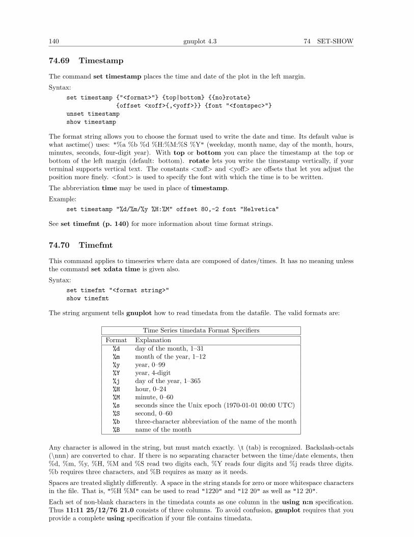
140 gnuplot 4.3 74 SET-SHOW
74.69 Timestamp
The command set timestamp places the time and date of the plot in the left margin.
Syntax:set timestamp {"<format>"} {top|bottom} {{no}rotate}
{offset <xoff>{,<yoff>}} {font "<fontspec>"}unset timestampshow timestamp
The format string allows you to choose the format used to write the date and time. Its default value iswhat asctime() uses: "%a %b %d %H:%M:%S %Y" (weekday, month name, day of the month, hours,minutes, seconds, four-digit year). With top or bottom you can place the timestamp at the top orbottom of the left margin (default: bottom). rotate lets you write the timestamp vertically, if yourterminal supports vertical text. The constants <xoff> and <yoff> are offsets that let you adjust theposition more finely. <font> is used to specify the font with which the time is to be written.
The abbreviation time may be used in place of timestamp.
Example:set timestamp "%d/%m/%y %H:%M" offset 80,-2 font "Helvetica"
See set timefmt (p. 140) for more information about time format strings.
74.70 Timefmt
This command applies to timeseries where data are composed of dates/times. It has no meaning unlessthe command set xdata time is given also.
Syntax:set timefmt "<format string>"show timefmt
The string argument tells gnuplot how to read timedata from the datafile. The valid formats are:
Time Series timedata Format SpecifiersFormat Explanation
%d day of the month, 1–31%m month of the year, 1–12%y year, 0–99%Y year, 4-digit%j day of the year, 1–365%H hour, 0–24%M minute, 0–60%s seconds since the Unix epoch (1970-01-01 00:00 UTC)%S second, 0–60%b three-character abbreviation of the name of the month%B name of the month
Any character is allowed in the string, but must match exactly. \t (tab) is recognized. Backslash-octals(\nnn) are converted to char. If there is no separating character between the time/date elements, then%d, %m, %y, %H, %M and %S read two digits each, %Y reads four digits and %j reads three digits.%b requires three characters, and %B requires as many as it needs.
Spaces are treated slightly differently. A space in the string stands for zero or more whitespace charactersin the file. That is, "%H %M" can be used to read "1220" and "12 20" as well as "12 20".
Each set of non-blank characters in the timedata counts as one column in the using n:n specification.Thus 11:11 25/12/76 21.0 consists of three columns. To avoid confusion, gnuplot requires that youprovide a complete using specification if your file contains timedata.
74 SET-SHOW gnuplot 4.3 141
Since gnuplot cannot read non-numerical text, if the date format includes the day or month in words,the format string must exclude this text. But it can still be printed with the "%a", "%A", "%b", or"%B" specifier: see set format (p. 102) for more details about these and other options for printingtimedata. (gnuplot will determine the proper month and weekday from the numerical values.)
See also set xdata (p. 143) and Time/date (p. 37) for more information.
Example:
set timefmt "%d/%m/%Y\t%H:%M"
tells gnuplot to read date and time separated by tab. (But look closely at your data — what began asa tab may have been converted to spaces somewhere along the line; the format string must match whatis actually in the file.) See also
time data demo.
74.71 Title
The set title command produces a plot title that is centered at the top of the plot. set title is a specialcase of set label.
Syntax:
set title {"<title-text>"} {offset <offset>} {font "<font>{,<size>}"}{{textcolor | tc} {<colorspec> | default}} {{no}enhanced}
show title
If <offset> is specified by either x,y or x,y,z the title is moved by the given offset. It may be preceded byfirst, second, graph, screen, or character to select the coordinate system. See coordinates (p. 20)for details. By default, the character coordinate system is used. For example, "set title offset 0,-1"will change only the y offset of the title, moving the title down by roughly the height of one character.The size of a character depends on both the font and the terminal.
<font> is used to specify the font with which the title is to be written; the units of the font <size>depend upon which terminal is used.
textcolor <colorspec> changes the color of the text. <colorspec> can be a linetype, an rgb color, ora palette mapping. See help for colorspec (p. 30) and palette (p. 126).
noenhanced requests that the title not be processed by the enhanced text mode parser, even if enhancedtext mode is currently active.
set title with no parameters clears the title.
See syntax (p. 36) for details about the processing of backslash sequences and the distinction betweensingle- and double-quotes.
74.72 Tmargin
The command set tmargin sets the size of the top margin. Please see set margin (p. 115) for details.
74.73 Trange
The set trange command sets the parametric range used to compute x and y values when in parametricor polar modes. Please see set xrange (p. 145) for details.
74.74 Urange
The set urange and set vrange commands set the parametric ranges used to compute x, y, and zvalues when in splot parametric mode. Please see set xrange (p. 145) for details.
142 gnuplot 4.3 74 SET-SHOW
74.75 Variables
The show variables command lists the current value of user-defined and internal variables. Gnuplotinternally defines variables whose names begin with GPVAL , MOUSE , FIT , and TERM .
Syntax:show variables # show variables that do not begin with GPVAL_show variables all # show all variables including those beginning GPVAL_show variables NAME # show only variables beginning with NAME
74.76 Version
The show version command lists the version of gnuplot being run, its last modification date, thecopyright holders, and email addresses for the FAQ, the gnuplot-info mailing list, and reporting bugs–inshort, the information listed on the screen when the program is invoked interactively.
Syntax:show version {long}
When the long option is given, it also lists the operating system, the compilation options used whengnuplot was installed, the location of the help file, and (again) the useful email addresses.
74.77 View
The set view command sets the viewing angle for splots. It controls how the 3D coordinates of theplot are mapped into the 2D screen space. It provides controls for both rotation and scaling of theplotted data, but supports orthographic projections only. It supports both 3D projection or orthogonal2D projection into a 2D plot-like map.
Syntax:set view <rot_x>{,{<rot_z>}{,{<scale>}{,<scale_z>}}}set view mapset view {no}equal {xy|xyz}show view
where <rot x> and <rot z> control the rotation angles (in degrees) in a virtual 3D coordinate systemaligned with the screen such that initially (that is, before the rotations are performed) the screen hori-zontal axis is x, screen vertical axis is y, and the axis perpendicular to the screen is z. The first rotationapplied is <rot x> around the x axis. The second rotation applied is <rot z> around the new z axis.
Command set view map is used to represent the drawing as a map. It can be used for contour plots,or for color pm3d maps. In the latter, take care that you properly use zrange and cbrange for inputdata point filtering and color range scaling, respectively.
<rot x> is bounded to the [0:180] range with a default of 60 degrees, while <rot z> is bounded tothe [0:360] range with a default of 30 degrees. <scale> controls the scaling of the entire splot, while<scale z> scales the z axis only. Both scales default to 1.0.
Examples:set view 60, 30, 1, 1set view ,,0.5
The first sets all the four default values. The second changes only scale, to 0.5.
74.77.1 Equal axes
The command set view equal xy forces the unit length of the x and y axes to be on the same scale, andchooses that scale so that the plot will fit on the page. The command set view equal xyz additionallysets the z axis scale to match the x and y axes; however there is no guarantee that the current z axis
74 SET-SHOW gnuplot 4.3 143
range will fit within the plot boundary. By default all three axes are scaled independently to fill theavailable area.
See also set ticslevel (p. 139).
74.78 Vrange
The set urange and set vrange commands set the parametric ranges used to compute x, y, and zvalues when in splot parametric mode. Please see set xrange (p. 145) for details.
74.79 X2data
The set x2data command sets data on the x2 (top) axis to timeseries (dates/times). Please see setxdata (p. 143).
74.80 X2dtics
The set x2dtics command changes tics on the x2 (top) axis to days of the week. Please see set xdtics(p. 144) for details.
74.81 X2label
The set x2label command sets the label for the x2 (top) axis. Please see set xlabel (p. 144).
74.82 X2mtics
The set x2mtics command changes tics on the x2 (top) axis to months of the year. Please see setxmtics (p. 145) for details.
74.83 X2range
The set x2range command sets the horizontal range that will be displayed on the x2 (top) axis. Pleasesee set xrange (p. 145) for details.
74.84 X2tics
The set x2tics command controls major (labelled) tics on the x2 (top) axis. Please see set xtics(p. 146) for details.
74.85 X2zeroaxis
The set x2zeroaxis command draws a line at the origin of the x2 (top) axis (y2 = 0). For details,please see set zeroaxis (p. 152).
74.86 Xdata
This command sets the datatype on the x axis to time/date. A similar command does the same thingfor each of the other axes.
Syntax:
set xdata {time}show xdata
144 gnuplot 4.3 74 SET-SHOW
The same syntax applies to ydata, zdata, x2data, y2data and cbdata.
The time option signals that the datatype is indeed time/date. If the option is not specified, thedatatype reverts to normal.
See set timefmt (p. 140) to tell gnuplot how to read date or time data. The time/date is convertedto seconds from start of the century. There is currently only one timefmt, which implies that all thetime/date columns must conform to this format. Specification of ranges should be supplied as quotedstrings according to this format to avoid interpretation of the time/date as an expression.
The function ’strftime’ (type "man strftime" on unix to look it up) is used to print tic-mark labels.gnuplot tries to figure out a reasonable format for this unless the set format x "string" has suppliedsomething that does not look like a decimal format (more than one ’%’ or neither %f nor %g).
See also Time/date (p. 37) for more information.
74.87 Xdtics
The set xdtics commands converts the x-axis tic marks to days of the week where 0=Sun and 6=Sat.Overflows are converted modulo 7 to dates. set noxdtics returns the labels to their default values.Similar commands do the same things for the other axes.
Syntax:
set xdticsunset xdticsshow xdtics
The same syntax applies to ydtics, zdtics, x2dtics, y2dtics and cbdtics.
See also the set format (p. 102) command.
74.88 Xlabel
The set xlabel command sets the x axis label. Similar commands set labels on the other axes.
Syntax:
set xlabel {"<label>"} {offset <offset>} {font "<font>{,<size>}"}{{textcolor | tc} {lt <line_type> | default}} {{no}enhanced}{rotate by <degrees>}
show xlabel
The same syntax applies to x2label, ylabel, y2label, zlabel and cblabel.
If <offset> is specified by either x,y or x,y,z the label is moved by the given offset. It may be preceded byfirst, second, graph, screen, or character to select the coordinate system. See coordinates (p. 20)for details. By default, the character coordinate system is used. For example, "set xlabel offset-1,0" will change only the x offset of the title, moving the label roughly one character width to the left.The size of a character depends on both the font and the terminal.
<font> is used to specify the font in which the label is written; the units of the font <size> dependupon which terminal is used.
textcolor lt <n> sets the text color to that of line type <n>.
noenhanced requests that the label text not be processed by the enhanced text mode parser, even ifenhanced text mode is currently active.
To clear a label, put no options on the command line, e.g., "set y2label".
The default positions of the axis labels are as follows:
xlabel: The x-axis label is centered below the bottom axis.
ylabel: The position of the y-axis label depends on the terminal, and can be one of the following threepositions:
74 SET-SHOW gnuplot 4.3 145
1. Horizontal text flushed left at the top left of the plot. Terminals that cannot rotate text will probablyuse this method. If set x2tics is also in use, the ylabel may overwrite the left-most x2tic label. Thismay be remedied by adjusting the ylabel position or the left margin.
2. Vertical text centered vertically at the left of the plot. Terminals that can rotate text will probablyuse this method.
3. Horizontal text centered vertically at the left of the plot. The EEPIC, LaTeX and TPIC drivers usethis method. The EEPIC driver will produce a stack of characters so as not to overwrite the plot. Withother drivers (such as LaTeX and TPIC), the user probably has to insert line breaks using \\ to preventthe ylabel from overwriting the plot.
zlabel: The z-axis label is centered along the z axis and placed in the space above the grid level.
cblabel: The color box axis label is centered along the box and placed below or right according tohorizontal or vertical color box gradient.
y2label: The y2-axis label is placed to the right of the y2 axis. The position is terminal-dependent inthe same manner as is the y-axis label.
x2label: The x2-axis label is placed above the top axis but below the plot title. It is also possible tocreate an x2-axis label by using new-line characters to make a multi-line plot title, e.g.,
set title "This is the title\n\nThis is the x2label"
Note that double quotes must be used. The same font will be used for both lines, of course.
The orientation (rotation angle) of the x, x2, y and y2 axis labels can be explicitly changed from thedefault setting, but this applies only to 2D plots and only on terminals that support text rotation.
If you are not satisfied with the default position of an axis label, use set label instead–that commandgives you much more control over where text is placed.
Please see syntax (p. 36) for further information about backslash processing and the difference betweensingle- and double-quoted strings.
74.89 Xmtics
The set xmtics command converts the x-axis tic marks to months of the year where 1=Jan and 12=Dec.Overflows are converted modulo 12 to months. The tics are returned to their default labels by unsetxmtics. Similar commands perform the same duties for the other axes.
Syntax:set xmticsunset xmticsshow xmtics
The same syntax applies to x2mtics, ymtics, y2mtics, zmtics and cbmtics.
See also the set format (p. 102) command.
74.90 Xrange
The set xrange command sets the horizontal range that will be displayed. A similar command existsfor each of the other axes, as well as for the polar radius r and the parametric variables t, u, and v.
Syntax:set xrange { [{{<min>}:{<max>}}] {{no}reverse} {{no}writeback} }
| restoreshow xrange
where <min> and <max> terms are constants, expressions or an asterisk to set autoscaling. If the dataare time/date, you must give the range as a quoted string according to the set timefmt format. Anyvalue omitted will not be changed.
146 gnuplot 4.3 74 SET-SHOW
The same syntax applies to yrange, zrange, x2range, y2range, cbrange, rrange, trange, urangeand vrange.
The reverse option reverses the direction of the axis, e.g., set xrange [0:1] reverse will produce anaxis with 1 on the left and 0 on the right. This is identical to the axis produced by set xrange [1:0],of course. reverse is intended primarily for use with autoscale.
The writeback option essentially saves the range found by autoscale in the buffers that would befilled by set xrange. This is useful if you wish to plot several functions together but have the rangedetermined by only some of them. The writeback operation is performed during the plot execution, soit must be specified before that command. To restore, the last saved horizontal range use set xrangerestore. For example,
set xrange [-10:10]set yrange [] writebackplot sin(x)set yrange restorereplot x/2
results in a yrange of [-1:1] as found only from the range of sin(x); the [-5:5] range of x/2 is ignored.Executing show yrange after each command in the above example should help you understand whatis going on.
In 2-d, xrange and yrange determine the extent of the axes, trange determines the range of theparametric variable in parametric mode or the range of the angle in polar mode. Similarly in parametric3-d, xrange, yrange, and zrange govern the axes and urange and vrange govern the parametricvariables.
In polar mode, rrange determines the radial range plotted. <rmin> acts as an additive constant to theradius, whereas <rmax> acts as a clip to the radius — no point with radius greater than <rmax> willbe plotted. xrange and yrange are affected — the ranges can be set as if the graph was of r(t)-rmin,with rmin added to all the labels.
Any range may be partially or totally autoscaled, although it may not make sense to autoscale a para-metric variable unless it is plotted with data.
Ranges may also be specified on the plot command line. A range given on the plot line will be used forthat single plot command; a range given by a set command will be used for all subsequent plots thatdo not specify their own ranges. The same holds true for splot.
Examples:
To set the xrange to the default:
set xrange [-10:10]
To set the yrange to increase downwards:
set yrange [10:-10]
To change zmax to 10 without affecting zmin (which may still be autoscaled):
set zrange [:10]
To autoscale xmin while leaving xmax unchanged:
set xrange [*:]
74.91 Xtics
Fine control of the major (labelled) tics on the x axis is possible with the set xtics command. The ticsmay be turned off with the unset xtics command, and may be turned on (the default state) with setxtics. Similar commands control the major tics on the y, z, x2 and y2 axes.
Syntax:
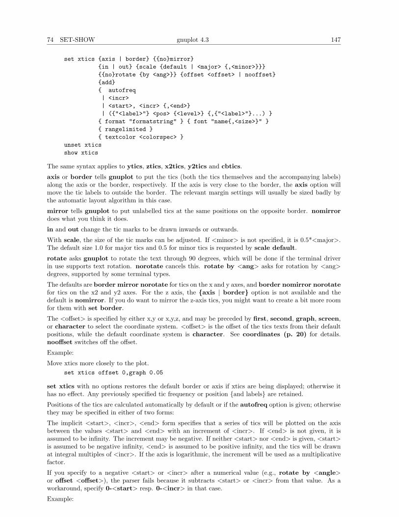
74 SET-SHOW gnuplot 4.3 147
set xtics {axis | border} {{no}mirror}{in | out} {scale {default | <major> {,<minor>}}}{{no}rotate {by <ang>}} {offset <offset> | nooffset}{add}{ autofreq| <incr>| <start>, <incr> {,<end>}| ({"<label>"} <pos> {<level>} {,{"<label>"}...) }{ format "formatstring" } { font "name{,<size>}" }{ rangelimited }{ textcolor <colorspec> }
unset xticsshow xtics
The same syntax applies to ytics, ztics, x2tics, y2tics and cbtics.
axis or border tells gnuplot to put the tics (both the tics themselves and the accompanying labels)along the axis or the border, respectively. If the axis is very close to the border, the axis option willmove the tic labels to outside the border. The relevant margin settings will usually be sized badly bythe automatic layout algorithm in this case.
mirror tells gnuplot to put unlabelled tics at the same positions on the opposite border. nomirrordoes what you think it does.
in and out change the tic marks to be drawn inwards or outwards.
With scale, the size of the tic marks can be adjusted. If <minor> is not specified, it is 0.5*<major>.The default size 1.0 for major tics and 0.5 for minor tics is requested by scale default.
rotate asks gnuplot to rotate the text through 90 degrees, which will be done if the terminal driverin use supports text rotation. norotate cancels this. rotate by <ang> asks for rotation by <ang>degrees, supported by some terminal types.
The defaults are border mirror norotate for tics on the x and y axes, and border nomirror norotatefor tics on the x2 and y2 axes. For the z axis, the {axis | border} option is not available and thedefault is nomirror. If you do want to mirror the z-axis tics, you might want to create a bit more roomfor them with set border.
The <offset> is specified by either x,y or x,y,z, and may be preceded by first, second, graph, screen,or character to select the coordinate system. <offset> is the offset of the tics texts from their defaultpositions, while the default coordinate system is character. See coordinates (p. 20) for details.nooffset switches off the offset.
Example:
Move xtics more closely to the plot.set xtics offset 0,graph 0.05
set xtics with no options restores the default border or axis if xtics are being displayed; otherwise ithas no effect. Any previously specified tic frequency or position {and labels} are retained.
Positions of the tics are calculated automatically by default or if the autofreq option is given; otherwisethey may be specified in either of two forms:
The implicit <start>, <incr>, <end> form specifies that a series of tics will be plotted on the axisbetween the values <start> and <end> with an increment of <incr>. If <end> is not given, it isassumed to be infinity. The increment may be negative. If neither <start> nor <end> is given, <start>is assumed to be negative infinity, <end> is assumed to be positive infinity, and the tics will be drawnat integral multiples of <incr>. If the axis is logarithmic, the increment will be used as a multiplicativefactor.
If you specify to a negative <start> or <incr> after a numerical value (e.g., rotate by <angle>or offset <offset>), the parser fails because it subtracts <start> or <incr> from that value. As aworkaround, specify 0-<start> resp. 0-<incr> in that case.
Example:
148 gnuplot 4.3 74 SET-SHOW
set xtics border offset 0,0.5 -5,1,5
Fails with ’invalid expression’ at the last comma.
set xtics border offset 0,0.5 0-5,1,5
or
set xtics offset 0,0.5 border -5,1,5
Sets tics at the border, tics text with an offset of 0,0.5 characters, and sets the start, increment, and endto -5, 1, and 5, as requested.
The set grid options ’front’, ’back’ and ’layerdefault’ affect the drawing order of the xtics, too.
Examples:
Make tics at 0, 0.5, 1, 1.5, ..., 9.5, 10.
set xtics 0,.5,10
Make tics at ..., -10, -5, 0, 5, 10, ...
set xtics 5
Make tics at 1, 100, 1e4, 1e6, 1e8.
set logscale x; set xtics 1,100,1e8
The explicit ("<label>" <pos> <level>, ...) form allows arbitrary tic positions or non-numeric ticlabels. In this form, the tics do not need to be listed in numerical order. Each tic has a position,optionally with a label. Note that the label is a string enclosed by quotes. It may be a constant string,such as "hello", may contain formatting information for converting the position into its label, such as"%3f clients", or may be empty, "". See set format (p. 102) for more information. If no string isgiven, the default label (numerical) is used.
An explicit tic mark has a third parameter, the "level". The default is level 0, a major tic. A level of 1generates a minor tic. If the level is specified, then the label must also be supplied.
Examples:
set xtics ("low" 0, "medium" 50, "high" 100)set xtics (1,2,4,8,16,32,64,128,256,512,1024)set ytics ("bottom" 0, "" 10, "top" 20)set ytics ("bottom" 0, "" 10 1, "top" 20)
In the second example, all tics are labelled. In the third, only the end tics are labelled. In the fourth,the unlabeled tic is a minor tic.
Normally if explicit tics are given, they are used instead of auto-generated tics. Conversely if you specifyset xtics auto or the like it will erase any previously specified explicit tics. You can mix explicit andauto- generated tics by using the keyword add, which must appear before the tic style being added.
Example:
set xtics 0,.5,10set xtics add ("Pi" 3.14159)
This will automatically generate tic marks every 0.5 along x, but will also add an explicit labeled ticmark at pi.
However they are specified, tics will only be plotted when in range.
Format (or omission) of the tic labels is controlled by set format, unless the explicit text of a label isincluded in the set xtics ("<label>") form.
Minor (unlabelled) tics can be added automatically by the set mxtics command, or at explicit positionsby the set xtics ("" <pos> 1, ...) form.
74 SET-SHOW gnuplot 4.3 149
74.91.1 Xtics time data
In case of timeseries data, axis tic position values must be given as quoted dates or times according tothe format timefmt. If the <start>, <incr>, <end> form is used, <start> and <end> must be givenaccording to timefmt, but <incr> must be in seconds. Times will be written out according to theformat given on set format, however.
Examples:set xdata timeset timefmt "%d/%m"set xtics format "%b %d"set xrange ["01/12":"06/12"]set xtics "01/12", 172800, "05/12"
set xdata timeset timefmt "%d/%m"set xtics format "%b %d"set xrange ["01/12":"06/12"]set xtics ("01/12", "" "03/12", "05/12")
Both of these will produce tics "Dec 1", "Dec 3", and "Dec 5", but in the second example the tic at"Dec 3" will be unlabelled.
74.91.2 Xtics rangelimited
This option limits both the auto-generated axis tic labels and the corresponding plot border to the rangeof values actually present in the data that has been plotted. Note that this is independent of the currentrange limits for the plot. For example, suppose that the data in "file.dat" all lies in the range 2 < y <4. Then the following commands will create a plot for which the left-hand plot border (y axis) is drawnfor only this portion of the total y range, and only the axis tics in this region are generated. I.e., theplot will be scaled to the full range on y, but there will be a gap between 0 and 2 on the left border andanother gap between 4 and 10. This style is sometimes refered to as a range-frame graph.
set border 3set yrange [0:10]set ytics nomirror rangelimitedplot "file.dat"
74.92 Xyplane
The set xyplane command adjusts the position at which the xy plane is drawn in a 3D plot. Thesynonym "set ticslevel" is accepted for backwards compatibility.
Syntax:set xyplane at <zvalue>set xyplane relative <frac>set ticslevel <frac># equivalent to set xyplane relativeshow xyplane
The form set xyplane relative <frac> places the xy plane below the range in Z, where the distancefrom the xy plane to Zmin is given as a fraction of the total range in z. The default value is 0.5.Negative values are permitted, but tic labels on the three axes may overlap. The older, deprecated, formset ticslevel is retained for backwards compatibility.
To place the xy-plane at a position ’pos’ on the z-axis, ticslevel may be set equal to (pos - zmin) /(zmin - zmax). However, this position will change if the z range is changed.
The alternative form set xyplane at <zvalue> fixes the placement of the xy plane at a specific Zvalue regardless of the current z range. Thus to force the x, y, and z axes to meet at a common originone would specify set xyplane at 0.
See also set view (p. 142), and set zeroaxis (p. 152).
150 gnuplot 4.3 74 SET-SHOW
74.93 Xzeroaxis
The set xzeroaxis command draws a line at y = 0. For details, please see set zeroaxis (p. 152).
74.94 Y2data
The set y2data command sets y2 (right-hand) axis data to timeseries (dates/times). Please see setxdata (p. 143).
74.95 Y2dtics
The set y2dtics command changes tics on the y2 (right-hand) axis to days of the week. Please see setxdtics (p. 144) for details.
74.96 Y2label
The set y2label command sets the label for the y2 (right-hand) axis. Please see set xlabel (p. 144).
74.97 Y2mtics
The set y2mtics command changes tics on the y2 (right-hand) axis to months of the year. Please seeset xmtics (p. 145) for details.
74.98 Y2range
The set y2range command sets the vertical range that will be displayed on the y2 (right-hand) axis.Please see set xrange (p. 145) for details.
74.99 Y2tics
The set y2tics command controls major (labelled) tics on the y2 (right-hand) axis. Please see set xtics(p. 146) for details.
74.100 Y2zeroaxis
The set y2zeroaxis command draws a line at the origin of the y2 (right-hand) axis (x2 = 0). Fordetails, please see set zeroaxis (p. 152).
74.101 Ydata
The set ydata commands sets y-axis data to timeseries (dates/times). Please see set xdata (p. 143).
74.102 Ydtics
The set ydtics command changes tics on the y axis to days of the week. Please see set xdtics (p. 144)for details.
74.103 Ylabel
This command sets the label for the y axis. Please see set xlabel (p. 144).

74 SET-SHOW gnuplot 4.3 151
74.104 Ymtics
The set ymtics command changes tics on the y axis to months of the year. Please see set xmtics(p. 145) for details.
74.105 Yrange
The set yrange command sets the vertical range that will be displayed on the y axis. Please see setxrange (p. 145) for details.
74.106 Ytics
The set ytics command controls major (labelled) tics on the y axis. Please see set xtics (p. 146) fordetails.
74.107 Yzeroaxis
The set yzeroaxis command draws a line at x = 0. For details, please see set zeroaxis (p. 152).
74.108 Zdata
The set zdata command sets zaxis data to timeseries (dates/times). Please see set xdata (p. 143).
74.109 Zdtics
The set zdtics command changes tics on the z axis to days of the week. Please see set xdtics (p. 144)for details.
74.110 Zzeroaxis
The set zzeroaxis command draws a line through (x=0,y=0). This has no effect on 2D plots, includingsplot with set view map. For details, please see set zeroaxis (p. 152) and set xyplane (p. 149).
74.111 Cbdata
Set color box axis data to timeseries (dates/times). Please see set xdata (p. 143).
74.112 Cbdtics
The set cbdtics command changes tics on the color box axis to days of the week. Please see set xdtics(p. 144) for details.
74.113 Zero
The zero value is the default threshold for values approaching 0.0.
Syntax:set zero <expression>show zero
gnuplot will not plot a point if its imaginary part is greater in magnitude than the zero threshold.This threshold is also used in various other parts of gnuplot as a (crude) numerical-error threshold.The default zero value is 1e-8. zero values larger than 1e-3 (the reciprocal of the number of pixels in atypical bitmap display) should probably be avoided, but it is not unreasonable to set zero to 0.0.

152 gnuplot 4.3 74 SET-SHOW
74.114 Zeroaxis
The x axis may be drawn by set xzeroaxis and removed by unset xzeroaxis. Similar commandsbehave similarly for the y, x2, y2, and z axes.
Syntax:set {x|x2|y|y2|z}zeroaxis { {linestyle | ls <line_style>}
| { linetype | lt <line_type>}{ linewidth | lw <line_width>}}
unset {x|x2|y|y2|z}zeroaxisshow {x|y|z}zeroaxis
By default, these options are off. The selected zero axis is drawn with a line of type <line type>and width <line width> (if supported by the terminal driver currently in use), or a user-defined style<line style>.
If no linetype is specified, any zero axes selected will be drawn using the axis linetype (linetype 0).
set zeroaxis is equivalent to set xzeroaxis; set yzeroaxis. Note that the z-axis must be set separatelyusing set zzeroaxis.
Examples:
To simply have the y=0 axis drawn visibly:
set xzeroaxis
If you want a thick line in a different color or pattern, instead:
set xzeroaxis linetype 3 linewidth 2.5
74.115 Zlabel
This command sets the label for the z axis. Please see set xlabel (p. 144).
74.116 Zmtics
The set zmtics command changes tics on the z axis to months of the year. Please see set xmtics(p. 145) for details.
74.117 Zrange
The set zrange command sets the range that will be displayed on the z axis. The zrange is used onlyby splot and is ignored by plot. Please see set xrange (p. 145) for details.
74.118 Ztics
The set ztics command controls major (labelled) tics on the z axis. Please see set xtics (p. 146) fordetails.
74.119 Cblabel
This command sets the label for the color box axis. Please see set xlabel (p. 144).
74.120 Cbmtics
The set cbmtics command changes tics on the color box axis to months of the year. Please see setxmtics (p. 145) for details.
76 SPLOT gnuplot 4.3 153
74.121 Cbrange
The set cbrange command sets the range of values which are colored using the current palette bystyles with pm3d, with image and with palette. Values outside of the color range use color of thenearest extreme.
If the cb-axis is autoscaled in splot, then the colorbox range is taken from zrange. Points drawn insplot ... pm3d|palette can be filtered by using different zrange and cbrange.
Please see set xrange (p. 145) for details on set cbrange (p. 153) syntax. See also set palette(p. 126) and set colorbox (p. 94).
74.122 Cbtics
The set cbtics command controls major (labelled) tics on the color box axis. Please see set xtics(p. 146) for details.
75 Shell
The shell command spawns an interactive shell. To return to gnuplot, type logout if using VMS, exitor the END-OF-FILE character if using Unix, endcli if using AmigaOS, or exit if using MS-DOS orOS/2.
There are two ways of spawning a shell command: using system command or via ! ($ if using VMS).The former command takes a string as a parameter and thus it can be used anywhere among othergnuplot commands, while the latter syntax requires to be the only command on the line. Control willreturn immediately to gnuplot after this command is executed. For example, in AmigaOS, MS-DOS orOS/2,
! dir
or
system "dir"
prints a directory listing and then returns to gnuplot.
Other examples of the former syntax:
system "date"; set time; plot "a.dat"print=1; if (print) replot; set out; system "lpr x.ps"
76 Splot
splot is the command for drawing 3D plots (well, actually projections on a 2D surface, but you knewthat). It can create a plot from functions or data read from files in a manner very similar to the plotcommand. splot provides only a single x, y, and z axis; there is no equivalent to the x2 and y2 secondaryaxes provided by plot.
See plot (p. 63) for features common to the plot (p. 63) command; only differences are discussed indetail here.
Syntax:
splot {<ranges>}{<iteration>}<function> | "<datafile>" {datafile-modifiers}}{<title-spec>} {with <style>}{, {definitions,} <function> ...}
154 gnuplot 4.3 76 SPLOT
where either a <function> or the name of a data file enclosed in quotes is supplied. The function canbe a mathematical expression, or a triple of mathematical expressions in parametric mode.
By default splot draws the xy plane completely below the plotted data. The offset between the lowestztic and the xy plane can be changed by set ticslevel. The orientation of a splot projection is controlledby set view. See set view (p. 142) and set ticslevel (p. 139) for more information.
The syntax for setting ranges on the splot command is the same as for plot. In non-parametric mode,the order in which ranges must be given is xrange, yrange, and zrange. In parametric mode, theorder is urange, vrange, xrange, yrange, and zrange.
The title option is the same as in plot. The operation of with is also the same as in plot, except thatthe plotting styles available to splot are limited to lines, points, linespoints, dots, and impulses;the error-bar capabilities of plot are not available for splot.
The datafile options have more differences.
See also show plot (p. 122).
76.1 Data-file
As for plot, discrete data contained in a file can be displayed by specifying the name of the data file,enclosed in quotes, on the splot command line.
Syntax:splot ’<file_name>’ {binary <binary list>}
{matrix}{index <index list>}{every <every list>}{using <using list>}
The special filenames "" and "-" are permitted, as in plot.
In brief, binary and matrix indicate that the data are in a special form, index selects which data setsin a multi-data-set file are to be plotted, every specifies which datalines (subsets) within a single dataset are to be plotted, and using determines how the columns within a single record are to be interpreted.
The options index and every behave the same way as with plot; using does so also, except that theusing list must provide three entries instead of two.
The plot options thru and smooth are not available for splot, but cntrparam and dgrid3d providelimited smoothing capabilities.
Data file organization is essentially the same as for plot, except that each point is an (x,y,z) triple. Ifonly a single value is provided, it will be used for z, the datablock number will be used for y, and theindex of the data point in the datablock will be used for x. If two or four values are provided, gnuplotuses the last value for calculating the color in pm3d plots. Three values are interpreted as an (x,y,z)triple. Additional values are generally used as errors, which can be used by fit.
Single blank records separate datablocks in a splot datafile; splot treats datablocks as the equivalentof function y-isolines. No line will join points separated by a blank record. If all datablocks contain thesame number of points, gnuplot will draw cross-isolines between datablocks, connecting correspondingpoints. This is termed "grid data", and is required for drawing a surface, for contouring (set contour)and hidden-line removal (set hidden3d). See also splot grid data (p. 157).
It is no longer necessary to specify parametric mode for three-column splots.
76.1.1 Binary matrix
Gnuplot can read matrix binary files by use of the option binary appearing without keyword qualifica-tions unique to general binary, i.e., array, record, format, or filetype. Other general binary keywordsfor translation should also apply to matrix binary. (See binary general (p. 66) for more details.)
In previous versions, gnuplot dynamically detected binary data files. It is now necessary to specify thekeyword binary directly after the filename.
76 SPLOT gnuplot 4.3 155
Single precision floats are stored in a binary file as follows:
<N+1> <y0> <y1> <y2> ... <yN><x0> <z0,0> <z0,1> <z0,2> ... <z0,N><x1> <z1,0> <z1,1> <z1,2> ... <z1,N>: : : : ... :
which are converted into triplets:
<x0> <y0> <z0,0><x0> <y1> <z0,1><x0> <y2> <z0,2>: : :<x0> <yN> <z0,N>
<x1> <y0> <z1,0><x1> <y1> <z1,1>: : :
These triplets are then converted into gnuplot iso-curves and then gnuplot proceeds in the usualmanner to do the rest of the plotting.
A collection of matrix and vector manipulation routines (in C) is provided in binary.c. The routine towrite binary data is
int fwrite_matrix(file,m,nrl,nrl,ncl,nch,row_title,column_title)
An example of using these routines is provided in the file bf test.c, which generates binary files for thedemo file demo/binary.dem.
The index keyword is not supported, since the file format allows only one surface per file. The everyand using filters are supported. using operates as if the data were read in the above triplet form.
See also binary general (p. 66) and
Binary File Splot Demo.
76.1.2 Example datafile
A simple example of plotting a 3D data file is
splot ’datafile.dat’
where the file "datafile.dat" might contain:
# The valley of the Gnu.0 0 100 1 100 2 10
1 0 101 1 51 2 10
2 0 102 1 12 2 10
3 0 103 1 03 2 10
156 gnuplot 4.3 76 SPLOT
Note that "datafile.dat" defines a 4 by 3 grid ( 4 rows of 3 points each ). Rows (datablocks) are separatedby blank records.
Note also that the x value is held constant within each dataline. If you instead keep y constant, andplot with hidden-line removal enabled, you will find that the surface is drawn ’inside-out’.
Actually for grid data it is not necessary to keep the x values constant within a datablock, nor is itnecessary to keep the same sequence of y values. gnuplot requires only that the number of points bethe same for each datablock. However since the surface mesh, from which contours are derived, connectssequentially corresponding points, the effect of an irregular grid on a surface plot is unpredictable andshould be examined on a case-by-case basis.
76.1.3 Matrix ascii
The matrix keyword (without a sequent binary keyword) in{s}plot ’a.dat’ matrix
indicates that data are stored in an ascii numbers matrix format.
The z-values are read in a row at a time, i. e.,z11 z12 z13 z14 ...z21 z22 z23 z24 ...z31 z32 z33 z34 ...
and so forth.
In 3D, the x- and y-indices of the matrix surface plot correspond to column and row indices of thematrix, respectively, being enumerated from 0. You can rescale or transform the axes as usual for a datafile with three columns by means of x=$1, y=$2, z=$3. For example
splot ’a.dat’ matrix using (1+$1/100):(1+$2*10):3
A blank line or comment line ends the matrix, and starts a new surface mesh. You can select amongthe meshes inside a file by the index option to the splot command, as usual.
See matrix (p. 156) for examples of plotting rows and columns of the matrix in a 2D plot.
76.1.4 Matrix
Datafile can be in an ascii or binary matrix format. The matrix flag indicates that the file is ascii,the binary or matrix binary stands for a binary format. For details, see matrix ascii (p. 156) andmatrix binary (p. 154).
Basic usage in splot:splot ’a.dat’ matrixsplot ’a.gpbin’ {matrix} binary
Advanced usage in splot:splot ’a.dat’ matrix using 1:2:3splot ’a.gpbin’ {matrix} binary using 1:2:3
allows to transform the axes coordinates and the z-data independently.
Usage in plot:plot ‘a.dat‘ matrixplot ‘a.dat‘ matrix using 1:3plot ’a.gpbin’ {matrix} binary using 1:3
will plot rows of the matrix, while using 2:3 will plot matrix columns, and using 1:2 the point coordinates(rather useless). Applying the every option you can specify explicit rows and columns.
Example – rescale axes of a matrix in an ascii file:splot ‘a.dat‘ matrix using (1+$1):(1+$2*10):3
77 SYSTEM gnuplot 4.3 157
Example – plot the 3rd row of a matrix in an ascii file:plot ’a.dat’ matrix using 1:3 every 1:999:1:2
(rows are enumerated from 0, thus 2 instead of 3).
76.2 Grid data
The 3D routines are designed for points in a grid format, with one sample, datapoint, at each mesh inter-section; the datapoints may originate from either evaluating a function, see set isosamples (p. 108), orreading a datafile, see splot datafile (p. 154). The term "isoline" is applied to the mesh lines for bothfunctions and data. Note that the mesh need not be rectangular in x and y, as it may be parameterizedin u and v, see set isosamples (p. 108).
However, gnuplot does not require that format. In the case of functions, ’samples’ need not be equal to’isosamples’, i.e., not every x-isoline sample need intersect a y-isoline. In the case of data files, if thereare an equal number of scattered data points in each datablock, then "isolines" will connect the pointsin a datablock, and "cross-isolines" will connect the corresponding points in each datablock to generatea "surface". In either case, contour and hidden3d modes may give different plots than if the points werein the intended format. Scattered data can be converted to a {different} grid format with set dgrid3d.
The contour code tests for z intensity along a line between a point on a y-isoline and the correspondingpoint in the next y-isoline. Thus a splot contour of a surface with samples on the x-isolines that do notcoincide with a y-isoline intersection will ignore such samples. Try:
set xrange [-pi/2:pi/2]; set yrange [-pi/2:pi/2]set style function lpset contourset isosamples 10,10; set samples 10,10;splot cos(x)*cos(y)set samples 4,10; replotset samples 10,4; replot
76.3 Splot overview
splot can display a surface as a collection of points, or by connecting those points. As with plot, thepoints may be read from a data file or result from evaluation of a function at specified intervals, see setisosamples (p. 108). The surface may be approximated by connecting the points with straight linesegments, see set surface (p. 137), in which case the surface can be made opaque with set hidden3d.The orientation from which the 3d surface is viewed can be changed with set view.
Additionally, for points in a grid format, splot can interpolate points having a common amplitude (seeset contour (p. 95)) and can then connect those new points to display contour lines, either directlywith straight-line segments or smoothed lines (see set cntrparam (p. 93)). Functions are alreadyevaluated in a grid format, determined by set isosamples and set samples, while file data must eitherbe in a grid format, as described in data-file, or be used to generate a grid (see set dgrid3d (p. 99)).
Contour lines may be displayed either on the surface or projected onto the base. The base projectionsof the contour lines may be written to a file, and then read with plot, to take advantage of plot’sadditional formatting capabilities.
77 System
system "command" executes "command" using the standard shell. See shell (p. 153). If called asa function, system("command") returns the resulting character stream from stdout as a string. Oneoptional trailing newline is ignored.
This can be used to import external functions into gnuplot scripts:f(x) = real(system(sprintf("somecommand %f", x)))
158 gnuplot 4.3 81 UPDATE
78 Test
This command graphically tests or presents terminal and palette capabilities.
Syntax:test {terminal | palette [rgb|rbg|grb|gbr|brg|bgr]}
test or test terminal creates a display of line and point styles and other useful things appropriate forand supported by the terminal you are just using.
test palette draws graphically profiles R(z),G(z),B(z), where 0<=z<=1, as calculated by the currentcolor palette. In other words, it is a beautiful plot you would have to construct from the result ofshow palette palette 256 float. The optional parameter, a permutation of letters rgb, determinesthe sequence of r,g,b profiles drawn one after the other — try this yourself for set palette gray. Thedefault sequence is rgb.
79 Undefine
Clear one or more previously defined user variables. This is useful in order to reset the state of a scriptcontaining an initialization test.
Example:
undefine foo foo1 foo2if (!exists("foo")) load "initialize.gp"
80 Unset
Options set using the set command may be returned to their default state by the corresponding unsetcommand. The unset command may contain an optional iteration clause. See iteration (p. 62).
Examples:set xtics mirror rotate by -45 0,10,100...unset xtics
# Unset labels numbered between 100 and 200unset for [i=100:200] label i
81 Update
This command writes the current values of the fit parameters into the given file, formatted as an initial-value file (as described in the fitsection). This is useful for saving the current values for later use or forrestarting a converged or stopped fit.
Syntax:update <filename> {<filename>}
If a second filename is supplied, the updated values are written to this file, and the original parameterfile is left unmodified.
Otherwise, if the file already exists, gnuplot first renames it by appending .old and then opens a new file.That is, "update ’fred’" behaves the same as "!rename fred fred.old; update ’fred.old’ ’fred’".[On DOS and other systems that use the twelve-character "filename.ext" naming convention, "ext" willbe "old" and "filename" will be related (hopefully recognizably) to the initial name. Renaming is notdone at all on VMS systems, since they use file-versioning.]
82 TERMINAL gnuplot 4.3 159
Please see fit (p. 54) for more information.
Part IV
Terminal types
82 Terminal
Gnuplot supports a large number of output formats. These are selected by choosing an appropriateterminal type, possibly with additional modifying options. See set terminal (p. 138).
This document may describe terminal types that are not available to you because they were not config-ured or installed on your system. To see a list of terminals available on a particular gnuplot installation,type ’set terminal’ with no modifiers.
82.1 Aed767
The aed512 and aed767 terminal drivers support AED graphics terminals. The two drivers differ onlyin their horizontal ranges, which are 512 and 768 pixels, respectively. Their vertical range is 575 pixels.There are no options for these drivers.
82.2 Aifm
NOTE: this terminal driver is outdated. Since Adobe Illustrator understands PostScript level 1 directly,you should use set terminal post level1 instead.
Several options may be set in aifm — the Adobe Illustrator 3.0+ driver.
Syntax:set terminal aifm {<color>} {"<fontname>"} {<fontsize>}
<color> is either color or monochrome; "<fontname>" is the name of a valid PostScript font;<fontsize> is the size of the font in PostScript points, before scaling by the set size command. Selectingdefault sets all options to their default values: monochrome, "Times-Roman", and 14pt.
Since AI does not really support multiple pages, multiple graphs will be drawn directly on top of oneanother. However, each graph will be grouped individually, making it easy to separate them inside AI(just pick them up and move them).
Examples:set term aifmset term aifm 22set size 0.7,1.4; set term aifm color "Times-Roman" 14
82.3 Amiga
The amiga terminal, for Commodore Amiga computers, allows the user to plot either to a screen(default), or, if Kickstart 3.0 or higher is installed, to a window on the current public screen. The fontand its size can also be selected.
Syntax:set terminal amiga {screen | window} {"<fontname>"} {<fontsize>}
The default font is 8-point "topaz".
The screen option uses a virtual screen, so it is possible that the graph will be larger than the screen.
160 gnuplot 4.3 82 TERMINAL
82.4 Apollo
The apollo terminal driver supports the Apollo Graphics Primitive Resource with rescaling after windowresizing. It has no options.
If a fixed-size window is desired, the gpr terminal may be used instead.
82.5 Aqua
This terminal relies on AquaTerm.app for display on Mac OS X.
Syntax:
set terminal aqua {<n>} {title "<wintitle>"} {size <x> <y>}{font "<fontname>{,<fontsize>}"}{{no}enhanced} {solid|dashed} {dl <dashlength>}}
where <n> is the number of the window to draw in (default is 0), <wintitle> is the name shown in thetitle bar (default "Figure <n>"), <x> <y> is the size of the plot (default is 846x594 pt = 11.75x8.25in).
Use <fontname> to specify the font to use (default is "Times-Roman"), and <fontsize> to specifythe font size (default is 14.0 pt). The old syntax {fname "<fontname>"} {fsize <fontsize>} is stillsupported.
The aqua terminal supports enhanced text mode (see enhanced (p. 21)), except for overprint. Fontsupport is limited to the fonts available on the system. Character encoding can be selected by setencoding and currently supports iso latin 1, iso latin 2, cp1250, and default which equals UTF8.
Lines can be drawn either solid or dashed, (default is solid) and the dash spacing can be modified by<dashlength> which is a multiplier > 0.
82.6 Be
gnuplot provides the be terminal type for use with X servers. This terminal type is set automaticallyat startup if the DISPLAY environment variable is set, if the TERM environment variable is set toxterm, or if the -display command line option is used.
Syntax:
set terminal be {reset} {<n>}
Multiple plot windows are supported: set terminal be <n> directs the output to plot window numbern. If n>0, the terminal number will be appended to the window title and the icon will be labeled gplt<n>. The active window may distinguished by a change in cursor (from default to crosshair.)
Plot windows remain open even when the gnuplot driver is changed to a different device. A plot windowcan be closed by pressing the letter q while that window has input focus, or by choosing close from awindow manager menu. All plot windows can be closed by specifying reset, which actually terminatesthe subprocess which maintains the windows (unless -persist was specified).
Plot windows will automatically be closed at the end of the session unless the -persist option was given.
The size or aspect ratio of a plot may be changed by resizing the gnuplot window.
Linewidths and pointsizes may be changed from within gnuplot with set linestyle.
For terminal type be, gnuplot accepts (when initialized) the standard X Toolkit options and resourcessuch as geometry, font, and name from the command line arguments or a configuration file. See the X(1)man page (or its equivalent) for a description of such options.
A number of other gnuplot options are available for the be terminal. These may be specified either ascommand-line options when gnuplot is invoked or as resources in the configuration file ".Xdefaults".They are set upon initialization and cannot be altered during a gnuplot session.
82 TERMINAL gnuplot 4.3 161
82.6.1 Command-line options
In addition to the X Toolkit options, the following options may be specified on the command line whenstarting gnuplot or as resources in your ".Xdefaults" file:
‘-mono‘ forces monochrome rendering on color displays.‘-gray‘ requests grayscale rendering on grayscale or color displays.
(Grayscale displays receive monochrome rendering by default.)‘-clear‘ requests that the window be cleared momentarily before a
new plot is displayed.‘-raise‘ raises plot window after each plot.
‘-noraise‘ does not raise plot window after each plot.‘-persist‘ plots windows survive after main gnuplot program exits.
The options are shown above in their command-line syntax. When entered as resources in ".Xdefaults",they require a different syntax.
Example:
gnuplot*gray: on
gnuplot also provides a command line option (-pointsize <v>) and a resource, gnuplot*pointsize:<v>, to control the size of points plotted with the points plotting style. The value v is a real number(greater than 0 and less than or equal to ten) used as a scaling factor for point sizes. For example,-pointsize 2 uses points twice the default size, and -pointsize 0.5 uses points half the normal size.
82.6.2 Monochrome options
For monochrome displays, gnuplot does not honor foreground or background colors. The default isblack-on-white. -rv or gnuplot*reverseVideo: on requests white-on-black.
82.6.3 Color resources
For color displays, gnuplot honors the following resources (shown here with their default values) or thegreyscale resources. The values may be color names as listed in the BE rgb.txt file on your system,hexadecimal RGB color specifications (see BE documentation), or a color name followed by a commaand an intensity value from 0 to 1. For example, blue, 0.5 means a half intensity blue.
gnuplot*background: whitegnuplot*textColor: blackgnuplot*borderColor: blackgnuplot*axisColor: blackgnuplot*line1Color: redgnuplot*line2Color: greengnuplot*line3Color: bluegnuplot*line4Color: magentagnuplot*line5Color: cyangnuplot*line6Color: siennagnuplot*line7Color: orangegnuplot*line8Color: coral
The command-line syntax for these is, for example,
Example:
gnuplot -background coral
162 gnuplot 4.3 82 TERMINAL
82.6.4 Grayscale resources
When -gray is selected, gnuplot honors the following resources for grayscale or color displays (shownhere with their default values). Note that the default background is black.
gnuplot*background: blackgnuplot*textGray: whitegnuplot*borderGray: gray50gnuplot*axisGray: gray50gnuplot*line1Gray: gray100gnuplot*line2Gray: gray60gnuplot*line3Gray: gray80gnuplot*line4Gray: gray40gnuplot*line5Gray: gray90gnuplot*line6Gray: gray50gnuplot*line7Gray: gray70gnuplot*line8Gray: gray30
82.6.5 Line resources
gnuplot honors the following resources for setting the width (in pixels) of plot lines (shown here withtheir default values.) 0 or 1 means a minimal width line of 1 pixel width. A value of 2 or 3 may improvethe appearance of some plots.
gnuplot*borderWidth: 2gnuplot*axisWidth: 0gnuplot*line1Width: 0gnuplot*line2Width: 0gnuplot*line3Width: 0gnuplot*line4Width: 0gnuplot*line5Width: 0gnuplot*line6Width: 0gnuplot*line7Width: 0gnuplot*line8Width: 0
gnuplot honors the following resources for setting the dash style used for plotting lines. 0 means a solidline. A two-digit number jk (j and k are >= 1 and <= 9) means a dashed line with a repeated patternof j pixels on followed by k pixels off. For example, ’16’ is a "dotted" line with one pixel on followedby six pixels off. More elaborate on/off patterns can be specified with a four-digit value. For example,’4441’ is four on, four off, four on, one off. The default values shown below are for monochrome displaysor monochrome rendering on color or grayscale displays. For color displays, the default for each is 0(solid line) except for axisDashes which defaults to a ’16’ dotted line.
gnuplot*borderDashes: 0gnuplot*axisDashes: 16gnuplot*line1Dashes: 0gnuplot*line2Dashes: 42gnuplot*line3Dashes: 13gnuplot*line4Dashes: 44gnuplot*line5Dashes: 15gnuplot*line6Dashes: 4441gnuplot*line7Dashes: 42gnuplot*line8Dashes: 13
82.7 Canvas
NB: The canvas terminal is EXPERIMENTAL, and may change before release.
82 TERMINAL gnuplot 4.3 163
Syntax:set terminal canvas {size <xsize>, <ysize>} {fsize <fontsize>}
{standalone | name ’<funcname>’}
where <xsize> and <ysize> set the size of the plot area in pixels. The default size in standalone modeis 600 by 400 pixels. The default font size is 10. NB: Only one font is available, the one loaded fromcanvastext.js
The default standalone mode creates an html page containing javascript code that renders the plotusing the HTML 5 canvas element. The html page links to a javascript library ’canvastext.js’. By defaultthis is a link to a local file, usually in directory /usr/local/share/gnuplot/<version>/js. You can changethis by setting environmental variable GNUPLOT JS DIR to either a local file or a general URL. Thelatter is usually appropriate if the plot is exported for viewing on remote client machines.
The name option creates a file containing only javascript. Both the javascript function it contains andthe id of the canvas element that it draws onto are taken from the following string parameter. Thecommands
set term canvas name ’fishplot’set output ’fishplot.js’
will create a file containing a javascript function fishplot() that will draw into a canvas with id=fishplot.An html page that invokes this javascript function must also load the canvastext.js function as describedabove. A minimal html file to wrap the fishplot created above might be:
<html><head>
<script src="canvastext.js"></script></head><body onload="fishplot();">
<script src="fishplot.js"></script><canvas id="fishplot" width=600 height=400>
<div id="err_msg">No support for HTML 5 canvas element</div></canvas>
</body></html>
82.8 Cgi
The cgi and hcgi terminal drivers support SCO CGI drivers. hcgi is for printers; the environmentvariable CGIPRNT must be set. cgi may be used for either a display or hardcopy; if the environmentvariable CGIDISP is set, then that display is used. Otherwise CGIPRNT is used.
These terminals have no options.
82.9 Cgm
The cgm terminal generates a Computer Graphics Metafile, Version 1. This file format is a subset ofthe ANSI X3.122-1986 standard entitled "Computer Graphics - Metafile for the Storage and Transfer ofPicture Description Information".
Syntax:set terminal cgm {color | monochrome} {solid | dashed} {{no}rotate}
{<mode>} {width <plot_width>} {linewidth <line_width>}{font "<fontname>,<fontsize>"}{<color0> <color1> <color2> ...}
solid draws all curves with solid lines, overriding any dashed patterns; <mode> is landscape, portrait,or default; <plot width> is the assumed width of the plot in points; <line width> is the line width in
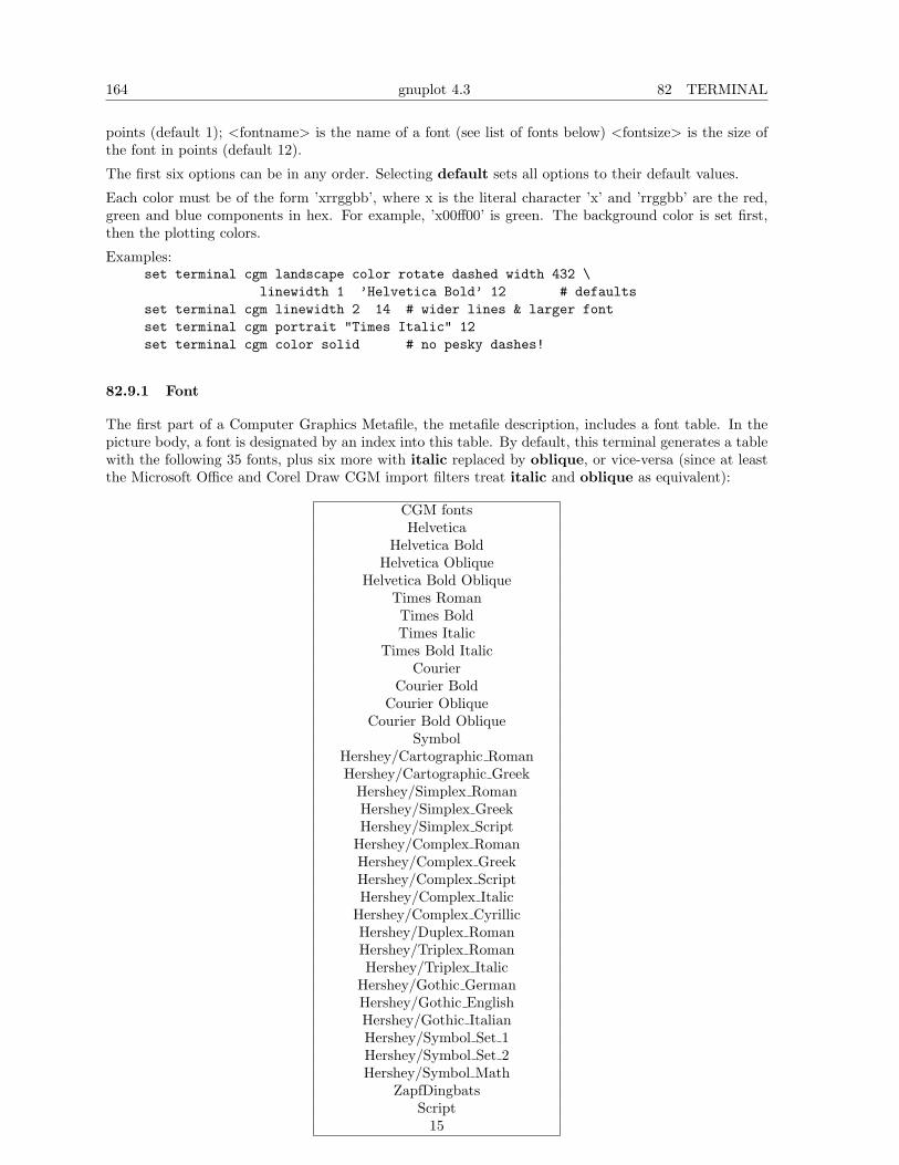
164 gnuplot 4.3 82 TERMINAL
points (default 1); <fontname> is the name of a font (see list of fonts below) <fontsize> is the size ofthe font in points (default 12).
The first six options can be in any order. Selecting default sets all options to their default values.
Each color must be of the form ’xrrggbb’, where x is the literal character ’x’ and ’rrggbb’ are the red,green and blue components in hex. For example, ’x00ff00’ is green. The background color is set first,then the plotting colors.
Examples:set terminal cgm landscape color rotate dashed width 432 \
linewidth 1 ’Helvetica Bold’ 12 # defaultsset terminal cgm linewidth 2 14 # wider lines & larger fontset terminal cgm portrait "Times Italic" 12set terminal cgm color solid # no pesky dashes!
82.9.1 Font
The first part of a Computer Graphics Metafile, the metafile description, includes a font table. In thepicture body, a font is designated by an index into this table. By default, this terminal generates a tablewith the following 35 fonts, plus six more with italic replaced by oblique, or vice-versa (since at leastthe Microsoft Office and Corel Draw CGM import filters treat italic and oblique as equivalent):
CGM fontsHelvetica
Helvetica BoldHelvetica Oblique
Helvetica Bold ObliqueTimes RomanTimes BoldTimes Italic
Times Bold ItalicCourier
Courier BoldCourier Oblique
Courier Bold ObliqueSymbol
Hershey/Cartographic RomanHershey/Cartographic Greek
Hershey/Simplex RomanHershey/Simplex GreekHershey/Simplex Script
Hershey/Complex RomanHershey/Complex GreekHershey/Complex ScriptHershey/Complex Italic
Hershey/Complex CyrillicHershey/Duplex RomanHershey/Triplex RomanHershey/Triplex Italic
Hershey/Gothic GermanHershey/Gothic EnglishHershey/Gothic ItalianHershey/Symbol Set 1Hershey/Symbol Set 2Hershey/Symbol Math
ZapfDingbatsScript
15
82 TERMINAL gnuplot 4.3 165
The first thirteen of these fonts are required for WebCGM. The Microsoft Office CGM import filterimplements the 13 standard fonts listed above, and also ’ZapfDingbats’ and ’Script’. However, the scriptfont may only be accessed under the name ’15’. For more on Microsoft import filter font substitutions,check its help file which you may find here:
C:\Program Files\Microsoft Office\Office\Cgmimp32.hlp
and/or its configuration file, which you may find here:
C:\Program Files\Common Files\Microsoft Shared\Grphflt\Cgmimp32.cfg
In the set term command, you may specify a font name which does not appear in the default font table.In that case, a new font table is constructed with the specified font as its first entry. You must ensurethat the spelling, capitalization, and spacing of the name are appropriate for the application that willread the CGM file. (Gnuplot and any MIL-D-28003A compliant application ignore case in font names.)If you need to add several new fonts, use several set term commands.
Example:
set terminal cgm ’Old English’set terminal cgm ’Tengwar’set terminal cgm ’Arabic’set output ’myfile.cgm’plot ...set output
You cannot introduce a new font in a set label command.
82.9.2 Fontsize
Fonts are scaled assuming the page is 6 inches wide. If the size command is used to change the aspectratio of the page or the CGM file is converted to a different width, the resulting font sizes will be scaledup or down accordingly. To change the assumed width, use the width option.
82.9.3 Linewidth
The linewidth option sets the width of lines in pt. The default width is 1 pt. Scaling is affected by theactual width of the page, as discussed under the fontsize and width options.
82.9.4 Rotate
The norotate option may be used to disable text rotation. For example, the CGM input filter for Wordfor Windows 6.0c can accept rotated text, but the DRAW editor within Word cannot. If you edit agraph (for example, to label a curve), all rotated text is restored to horizontal. The Y axis label will thenextend beyond the clip boundary. With norotate, the Y axis label starts in a less attractive location,but the page can be edited without damage. The rotate option confirms the default behavior.
82.9.5 Solid
The solid option may be used to disable dashed line styles in the plots. This is useful when color isenabled and the dashing of the lines detracts from the appearance of the plot. The dashed optionconfirms the default behavior, which gives a different dash pattern to each line type.
82.9.6 Size
Default size of a CGM plot is 32599 units wide and 23457 units high for landscape, or 23457 units wideby 32599 units high for portrait.
166 gnuplot 4.3 82 TERMINAL
82.9.7 Width
All distances in the CGM file are in abstract units. The application that reads the file determines thesize of the final plot. By default, the width of the final plot is assumed to be 6 inches (15.24 cm). Thisdistance is used to calculate the correct font size, and may be changed with the width option. Thekeyword should be followed by the width in points. (Here, a point is 1/72 inch, as in PostScript. Thisunit is known as a "big point" in TeX.) Gnuplot expressions can be used to convert from other units.
Example:set terminal cgm width 432 # defaultset terminal cgm width 6*72 # same as aboveset terminal cgm width 10/2.54*72 # 10 cm wide
82.9.8 Nofontlist
The default font table includes the fonts recommended for WebCGM, which are compatible with theComputer Graphics Metafile input filter for Microsoft Office and Corel Draw. Another application mightuse different fonts and/or different font names, which may not be documented. The nofontlist (synonymwinword6) option deletes the font table from the CGM file. In this case, the reading application shoulduse a default table. Gnuplot will still use its own default font table to select font indices. Thus, ’Helvetica’will give you an index of 1, which should get you the first entry in your application’s default font table.’Helvetica Bold’ will give you its second entry, etc.
82.10 Corel
The corel terminal driver supports CorelDraw.
Syntax:set terminal corel { default
| {monochrome | color{"<font>" {<fontsize>
{<xsize> <ysize> {<linewidth> }}}}}
where the fontsize and linewidth are specified in points and the sizes in inches. The defaults aremonochrome, "SwitzerlandLight", 22, 8.2, 10 and 1.2.
82.11 Debug
This terminal is provided to allow for the debugging of gnuplot. It is likely to be of use only for userswho are modifying the source code.
82.12 Dospc
The dospc terminal driver supports PCs with arbitrary graphics boards, which will be automaticallydetected. It should be used only if you are not using the gcc or Zortec C/C++ compilers.
82.13 Dumb
The dumb terminal driver has an optional size specification and trailing linefeed control.
Syntax:set terminal dumb {[no]feed} {<xsize> <ysize>}
{[no]enhanced}
where <xsize> and <ysize> set the size of the dumb terminals. Default is 79 by 24. The last newlineis printed only if feed is enabled.
Examples:
82 TERMINAL gnuplot 4.3 167
set term dumb nofeedset term dumb 79 49 # VGA screen---why would anyone do that?
82.14 Dxf
The dxf terminal driver creates pictures that can be imported into AutoCad (Release 10.x). It has nooptions of its own, but some features of its plots may be modified by other means. The default size is120x80 AutoCad units, which can be changed by set size. dxf uses seven colors (white, red, yellow,green, cyan, blue and magenta), which can be changed only by modifying the source file. If a black-and-white plotting device is used, the colors are mapped to differing line thicknesses. See the description ofthe AutoCad print/plot command.
82.15 Dxy800a
This terminal driver supports the Roland DXY800A plotter. It has no options.
82.16 Eepic
The eepic terminal driver supports the extended LaTeX picture environment. It is an alternative to thelatex driver.
The output of this terminal is intended for use with the "eepic.sty" macro package for LaTeX. To use it,you need "eepic.sty", "epic.sty" and a printer driver that supports the "tpic" \specials. If your printerdriver doesn’t support those \specials, "eepicemu.sty" will enable you to use some of them. dvips anddvipdfm do support the "tpic" \specials.
Syntax:
set terminal eepic {color, dashed, rotate, small, tiny, default, <fontsize>}
Options: You can give options in any order you wish. ’color’ causes gnuplot to produce \color{...}commands so that the graphs are colored. Using this option, you must include \usepackage{color}in the preambel of your latex document. ’dashed’ will allow dashed line types; without this option,only solid lines with varying thickness will be used. ’dashed’ and ’color’ are mutually exclusive; if’color’ is specified, then ’dashed’ will be ignored. ’rotate’ will enable true rotated text (by 90 degrees).Otherwise, rotated text will be typeset with letters stacked above each other. If you use this optionyou must include \usepackage{graphicx} in the preamble. ’small’ will use \scriptsize symbols as pointmarkers (Probably does not work with TeX, only LaTeX2e). Default is to use the default math size.’tiny’ uses \scriptscriptstyle symbols. ’default’ resets all options to their defaults = no color, no dashedlines, pseudo-rotated (stacked) text, large point symbols. <fontsize> is a number which specifies thefont size inside the picture environment; the unit is pt (points), i.e., 10 pt equals approx. 3.5 mm. Iffontsize is not specified, then all text inside the picture will be set in \footnotesize.
Notes: Remember to escape the # character (or other chars meaningful to (La-)TeX) by \\ (2 back-slashes). It seems that dashed lines become solid lines when the vertices of a plot are too close. (I donot know if that is a general problem with the tpic specials, or if it is caused by a bug in eepic.sty ordvips/dvipdfm.) The default size of an eepic plot is 5x3 inches, which can be scaled by ’set size a,b’.Points, among other things, are drawn using the LaTeX commands "\Diamond", "\Box", etc. Thesecommands no longer belong to the LaTeX2e core; they are included in the latexsym package, which ispart of the base distribution and thus part of any LaTeX implementation. Please do not forget to usethis package. Instead of latexsym, you can also include the amssymb package. All drivers for LaTeXoffer a special way of controlling text positioning: If any text string begins with ’{’, you also need toinclude a ’}’ at the end of the text, and the whole text will be centered both horizontally and vertically.If the text string begins with ’[’, you need to follow this with a position specification (up to two out oft,b,l,r), ’]{’, the text itself, and finally ’}’. The text itself may be anything LaTeX can typeset as anLR-box. ’\rule{}{}’s may help for best positioning.
Examples: set term eepic
168 gnuplot 4.3 82 TERMINAL
output graphs as eepic macros inside a picture environment;\input the resulting file in your LaTeX document.
set term eepic color tiny rotate 8eepic macros with \color macros, \scripscriptsize point markers,true rotated text, and all text set with 8pt.
About label positioning: Use gnuplot defaults (mostly sensible, but sometimes not really best):set title ’\LaTeX\ -- $ \gamma $’
Force centering both horizontally and vertically:set label ’{\LaTeX\ -- $ \gamma $}’ at 0,0
Specify own positioning (top here):set xlabel ’[t]{\LaTeX\ -- $ \gamma $}’
The other label – account for long ticlabels:set ylabel ’[r]{\LaTeX\ -- $ \gamma $\rule{7mm}{0pt}}’
82.17 Emf
The emf terminal generates an Enhanced Metafile Format file. This file format is recognized by manyWindows applications.
Syntax:set terminal emf {color | monochrome} {solid | dashed}
{enhanced {noproportional}}{linewidth <LW>} {dashlength <DL>} {size XX,YY}{"<fontname>"} {<fontsize>} #old syntax{font "<fontname>,<fontsize>"} #new syntax
In monochrome mode successive line types cycle through dash patterns. In color mode successive linetypes use successive colors, and only after all 8 default colors are exhausted is the dash pattern incre-mented. solid draws all curves with solid lines, overriding any dashed patterns; linewidth <factor>multiplies all line widths by this factor. dashlength <factor> is useful for thick lines. <fontname> isthe name of a font; and <fontsize> is the size of the font in points.
The nominal size of the output image defaults to 1024x768 in arbitrary units. You may specify a differentnominal size using the size option.
Enhanced text mode tries to approximate proportional character spacing. If you are using a monospacedfont, or don’t like the approximation, you can turn off this correction using the noproportional option.
The default settings are color dashed font "Arial,12" size 1024,768 Selecting default sets alloptions to their default values.
Examples:set terminal emf ’Times Roman Italic’ 12set terminal emf color solid # no pesky dashes!
82.18 Emxvga
The emxvga, emxvesa and vgal terminal drivers support PCs with SVGA, vesa SVGA andVGA graphics boards, respectively. They are intended to be compiled with "emx-gcc" undereither DOS or OS/2. They also need VESA and SVGAKIT maintained by Johannes Martin([email protected]) with additions by David J. Liu ([email protected]).
Syntax:set terminal emxvgaset terminal emxvesa {vesa-mode}set terminal vgal
The only option is the vesa mode for emxvesa, which defaults to G640x480x256.
82 TERMINAL gnuplot 4.3 169
82.19 Epslatex
The epslatex driver generates output for further processing by LaTeX.
Syntax:
set terminal epslatex {default}set terminal epslatex {standalone | input}
{oldstyle | newstyle}{level1 | leveldefault}{color | colour | monochrome}{solid | dashed}{dashlength | dl <DL>}{linewidth | lw <LW>}{rounded | butt}{palfuncparam <samples>{,<maxdeviation>}}{size <XX>{unit},<YY>{unit}}{header <header> | noheader}{blacktext | colortext | colourtext}{{font} "fontname{,fontsize}" {<fontsize>}}
The epslatex terminal prints a plot as terminal postscript eps but transfers the texts to LaTeX insteadof including in the PostScript code. Thus, many options are the same as in the postscript terminal.
From version 4.0 to 4.1, some changes have been invoked into the default appearance of the epslatexterminal to reach better consistency with the postscript terminal: The plot size has been changed from5 x 3 inches to 5 x 3.5 inches; the character width is now estimated to be 60% of the font size while theold epslatex terminal used 50%; now, the larger number of postscript linetypes and symbols are used.To reach an appearance that is nearly identical to the old one specify the option oldstyle. (In fact somesmall differences remain: the symbol sizes are slightly different, the tics are half as large as in the oldterminal which can be changed using set tics scale, and the arrows have all features as in the postscriptterminal.)
If you see the error message
"Can’t find PostScript prologue file ... "
Please see and follow the instructions in postscript prologue (p. 194).
The option color enables color, while monochrome prefers black and white drawing elements. Further,monochrome uses gray palette but it does not change color of objects specified with an explicitcolorspec. solid draws all plots with solid lines, overriding any dashed patterns. dashlength or dlscales the length of the dashed-line segments by <DL>, which is a floating-point number greater thanzero. linewidth or lw scales all linewidths by <LW>.
By default the generated PostScript code uses language features that were introduced in PostScript Level2, notably filters and pattern-fill of irregular objects such as filledcurves. PostScript Level 2 features areconditionally protected so that PostScript Level 1 interpreters do not issue errors but, rather, displaya message or a PostScript Level 1 approximation. The level1 option substitutes PostScript Level 1approximations of these features and uses no PostScript Level 2 code. This may be required by someold printers and old versions of Adobe Illustrator. The flag level1 can be toggled later by editing asingle line in the PostScript output file to force PostScript Level 1 interpretation. In the case of filescontaining level 2 code, the above features will not appear or will be replaced by a note when this flag isset or when the interpreting program does not indicate that it understands level 2 PostScript or higher.
rounded sets line caps and line joins to be rounded; butt is the default, butt caps and mitered joins;
palfuncparam controls how set palette functions are encoded as gradients in the output. Analyticcolor component functions (set via set palette functions) are encoded as linear interpolated gradientsin the postscript output: The color component functions are sampled at <samples> points and all pointsare removed from this gradient which can be removed without changing the resulting colors by more than<maxdeviation>. For almost every useful palette you may savely leave the defaults of <samples>=2000and <maxdeviation>=0.003 untouched.
170 gnuplot 4.3 82 TERMINAL
The default size for postscript output is 10 inches x 7 inches. The default for eps output is 5 x 3.5 inches.The size option changes this to whatever the user requests. By default the X and Y sizes are taken tobe in inches, but other units are possibly (currently only cm). The BoundingBox of the plot is correctlyadjusted to contain the resized image. Screen coordinates always run from 0.0 to 1.0 along the fulllength of the plot edges as specified by the size option. NB: this is a change from the previouslyrecommended method of using the set size command prior to setting the terminal type.The old method left the BoundingBox unchanged and screen coordinates did not correspond to theactual limits of the plot.
blacktext forces all text to be written in black even in color mode;
The epslatex driver offers a special way of controlling text positioning: (a) If any text string beginswith ’{’, you also need to include a ’}’ at the end of the text, and the whole text will be centered bothhorizontally and vertically by LaTeX. (b) If the text string begins with ’[’, you need to continue it with:a position specification (up to two out of t,b,l,r,c), ’]{’, the text itself, and finally, ’}’. The text itself maybe anything LaTeX can typeset as an LR-box. \rule{}{}’s may help for best positioning. See also thedocumentation for the pslatex (p. 194) terminal driver. To create multiline labels, use \shortstack,for exampleset ylabel ’[r]{\shortstack{first line \\ second line}}’
The back option of set label commands is handled slightly different than in other terminals. Labelsusing ’back’ are printed behind all other elements of the plot while labels using ’front’ are printed aboveeverything else.
The driver produces two different files, one for the eps part of the figure and one for the LaTeX part.The name of the LaTeX file is taken from the set output command. The name of the eps file is derivedby replacing the file extension (normally .tex) with .eps instead. There is no LaTeX output if no outputfile is given! Remember to close the output file before next plot unless in multiplot mode.
In your LaTeX documents use ’\input{filename}’ to include the figure. The .eps file is included by thecommand \includegraphics{...}, so you must also include \usepackage{graphicx} in the LaTeX preamble.If you want to use coloured text (option textcolour) you also have to include \usepackage{color} in theLaTeX preamble.
Pdf files can be made from the eps file using ’epstopdf’. If the graphics package is properly configured,the LaTeX files can also be processed by pdflatex without changes, using the pdf files instead of theeps files. The behaviour concerning font selection depends on the header mode. In all cases, the givenfont size is used for the calculation of proper spacing. When not using the standalone mode the actualLaTeX font and font size at the point of inclusion is taken, so use LaTeX commands for changing fonts.If you use e.g. 12pt as font size for your LaTeX document, use ’"" 12’ as options. The font name isignored. If using standalone the given font and font size are used, see below for a detailed description.
If text is printed coloured is controlled by the TeX booleans \ifGPcolor and \ifGPblacktext. Only if\ifGPcolor is true and \ifGPblacktext is false, text is printed coloured. You may either change them inthe generated TeX file or provide them globally in your TeX file, for example by using\newif\ifGPblacktext\GPblacktexttrue
in the preamble of your document. The local assignment is only done if no global value is given.
When using the epslatex terminal give the name of the TeX file in the set output command includingthe file extension (normally ".tex"). The eps filename is generated by replacing the extension by ".eps".
If using the standalone mode a complete LaTeX header is added to the LaTeX file; and "-inc" is addedto the filename of the eps file. The standalone mode generates a TeX file that produces output withthe correct size when using dvips, pdfTeX, or VTeX. The default, input, generates a file that has to beincluded into a LaTeX document using the \input command.
If a font other than "" or "default" is given it is interpreted as LaTeX font name. It containsup to three parts, separated by a comma: ’fontname,fontseries,fontshape’. If the default fontshapeor fontseries are requested, they can be omitted. Thus, the real syntax for the fontname is ’[font-name][,fontseries][,fontshape]’. The naming convention for all parts is given by the LaTeX font scheme.The fontname is 3 to 4 characters long and is built as follows: One character for the font vendor, two

82 TERMINAL gnuplot 4.3 171
characters for the name of the font, and optionally one additional character for special fonts, e.g., ’j’ forfonts with old-style numerals or ’x’ for expert fonts. The names of many fonts is described in
http://www.tug.org/fontname/fontname.pdf
For example, ’cmr’ stands for Computer Modern Roman, ’ptm’ for Times-Roman, and ’phv’ for Helvetica.The font series denotes the thickness of the glyphs, in most cases ’m’ for normal ("medium") and ’bx’or ’b’ for bold fonts. The font shape is ’n’ for upright, ’it’ for italics, ’sl’ for slanted, or ’sc’ for smallcaps, in general. Some fonts may provide different font series or shapes.
Examples:
Use Times-Roman boldface (with the same shape as in the surrounding text):set terminal epslatex ’ptm,bx’
Use Helvetica, boldface, italics:set terminal epslatex ’phv,bx,it’
Continue to use the surrounding font in slanted shape:set terminal epslatex ’,,sl’
Use small capitals:set terminal epslatex ’,,sc’
By this method, only text fonts are changed. If you also want to change the math fonts you have to usethe "gnuplot.cfg" file or the header option, described below.
In standalone mode, the font size is taken from the given font size in the set terminal command. Tobe able to use a specified font size, a file "size<size>.clo" has to reside in the LaTeX search path. Bydefault, 10pt, 11pt, and 12pt are supported. If the package "extsizes" is installed, 8pt, 9pt, 14pt, 17pt,and 20pt are added.
The header option takes a string as argument. This string is written into the generated LaTeX file.If using the standalone mode, it is written into the preamble, directly before the \begin{document}command. In the input mode, it is placed directly after the \begingroup command to ensure that allsettings are local to the plot.
Examples:
Use T1 fontencoding, change the text and math font to Times-Roman as well as the sans-serif font toHelvetica:
set terminal epslatex standalone header \"\\usepackage[T1]{fontenc}\n\\usepackage{mathptmx}\n\\usepackage{helvet}"
Use a boldface font in the plot, not influencing the text outside the plot:set terminal epslatex input header "\\bfseries"
If the file "gnuplot.cfg" is found by LaTeX it is input in the preamble the LaTeX document, when usingstandalone mode. It can be used for further settings, e.g., changing the document font to Times-Roman,Helvetica, and Courier, including math fonts (handled by "mathptmx.sty"):
\usepackage{mathptmx}\usepackage[scaled=0.92]{helvet}\usepackage{courier}
The file "gnuplot.cfg" is loaded before the header information given by the header command. Thus,you can use header to overwrite some of settings performed using "gnuplot.cfg"
82.20 Epson 180dpi
This driver supports a family of Epson printers and derivatives.
epson 180dpi and epson 60dpi are drivers for Epson LQ-style 24-pin printers with resolutions of 180and 60 dots per inch, respectively.
172 gnuplot 4.3 82 TERMINAL
epson lx800 is a generic 9-pin driver appropriate for printers like the Epson LX-800, the Star NL-10and NX-1000, the PROPRINTER, and so forth.
nec cp6 is generic 24-pin driver that can be used for printers like the NEC CP6 and the Epson LQ-800.
The okidata driver supports the 9-pin OKIDATA 320/321 Standard printers.
The starc driver is for the Star Color Printer.
The tandy 60dpi driver is for the Tandy DMP-130 series of 9-pin, 60-dpi printers.
The dpu414 driver is for the Seiko DPU-414 thermal printer.
nec cp6 has the options:
Syntax:set terminal nec_cp6 {monochrome | colour | draft}
which defaults to monochrome.
dpu414 has the options:
Syntax:set terminal dpu414 {small | medium | large} {normal | draft}
which defaults to medium (=font size) and normal. Preferred combinations are medium normal andsmall draft.
82.21 Excl
The excl terminal driver supports Talaris printers such as the EXCL Laser printer and the 1590. It hasno options.
82.22 Fig
The fig terminal device generates output in the Fig graphics language.
Syntax:set terminal fig {monochrome | color}
{landscape | portrait}{small | big | size <xsize> <ysize>}{metric | inches}{pointsmax <max_points>}{solid | dashed}{font <fontname>} {fontsize <fsize>}{textnormal | {textspecial texthidden textrigid}}{{thickness|linewidth} <units>}{depth <layer>}{version <number>}
monochrome and color determine whether the picture is black-and-white or color. small and bigproduce a 5x3 or 8x5 inch graph in the default landscape mode and 3x5 or 5x8 inches in portrait mode.size sets (overrides) the size of the drawing area to <xsize>*<ysize> in units of inches or centimetersdepending on the inches or metric setting in effect. The latter settings is also used as default units forediting with "xfig".
pointsmax <max points> sets the maximum number of points per polyline.
solid inhibits automatic usage of dashed lines when solid linestyles are used up, which otherwise occurs.
fontsize sets the size of the text font to <fsize> points. textnormal resets the text flags and selectspostscript fonts, textspecial sets the text flags for LaTeX specials, texthidden sets the hidden flagand textrigid the rigid flag.
depth sets the default depth layer for all lines and text. The default depth is 10 to leave room foradding material with "xfig" on top of the plot.
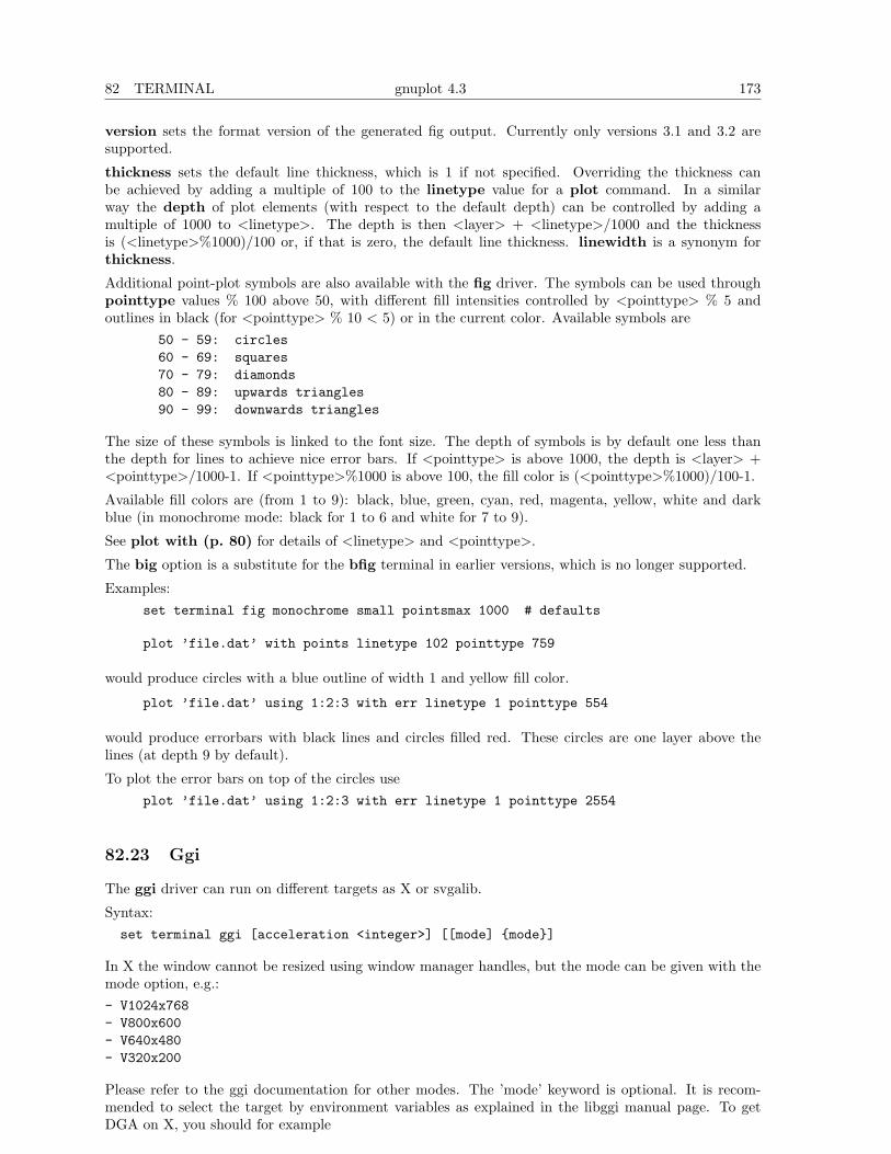
82 TERMINAL gnuplot 4.3 173
version sets the format version of the generated fig output. Currently only versions 3.1 and 3.2 aresupported.
thickness sets the default line thickness, which is 1 if not specified. Overriding the thickness canbe achieved by adding a multiple of 100 to the linetype value for a plot command. In a similarway the depth of plot elements (with respect to the default depth) can be controlled by adding amultiple of 1000 to <linetype>. The depth is then <layer> + <linetype>/1000 and the thicknessis (<linetype>%1000)/100 or, if that is zero, the default line thickness. linewidth is a synonym forthickness.
Additional point-plot symbols are also available with the fig driver. The symbols can be used throughpointtype values % 100 above 50, with different fill intensities controlled by <pointtype> % 5 andoutlines in black (for <pointtype> % 10 < 5) or in the current color. Available symbols are
50 - 59: circles60 - 69: squares70 - 79: diamonds80 - 89: upwards triangles90 - 99: downwards triangles
The size of these symbols is linked to the font size. The depth of symbols is by default one less thanthe depth for lines to achieve nice error bars. If <pointtype> is above 1000, the depth is <layer> +<pointtype>/1000-1. If <pointtype>%1000 is above 100, the fill color is (<pointtype>%1000)/100-1.
Available fill colors are (from 1 to 9): black, blue, green, cyan, red, magenta, yellow, white and darkblue (in monochrome mode: black for 1 to 6 and white for 7 to 9).
See plot with (p. 80) for details of <linetype> and <pointtype>.
The big option is a substitute for the bfig terminal in earlier versions, which is no longer supported.
Examples:set terminal fig monochrome small pointsmax 1000 # defaults
plot ’file.dat’ with points linetype 102 pointtype 759
would produce circles with a blue outline of width 1 and yellow fill color.
plot ’file.dat’ using 1:2:3 with err linetype 1 pointtype 554
would produce errorbars with black lines and circles filled red. These circles are one layer above thelines (at depth 9 by default).
To plot the error bars on top of the circles useplot ’file.dat’ using 1:2:3 with err linetype 1 pointtype 2554
82.23 Ggi
The ggi driver can run on different targets as X or svgalib.
Syntax:set terminal ggi [acceleration <integer>] [[mode] {mode}]
In X the window cannot be resized using window manager handles, but the mode can be given with themode option, e.g.:- V1024x768- V800x600- V640x480- V320x200
Please refer to the ggi documentation for other modes. The ’mode’ keyword is optional. It is recom-mended to select the target by environment variables as explained in the libggi manual page. To getDGA on X, you should for example
174 gnuplot 4.3 82 TERMINAL
bash> export GGI_DISPLAY=DGAcsh> setenv GGI_DISPLAY DGA
’acceleration’ is only used for targets which report relative pointer motion events (e.g. DGA) and is astrictly positive integer multiplication factor for the relative distances. The default for acceleration is 7.
Examples:set term ggi acc 10set term ggi acc 1 mode V1024x768set term ggi V1024x768
82.24 Gif
Syntax:set terminal gif
{tiny | small | medium | large | giant}{{no}transparent} {{no}enhanced}{linewidth <lw>} {dashlength <dl>}{font <face> {<pointsize>}}{animate {delay <time>} {{no}optimize}}{size <x>,<y>} {{no}crop}{<color0> <color1> <color2> ...}
GIF images are created using libgd, with optional support for TrueType fonts via libfreetype.
GIF plots may be conveniently viewed by piping the output to the ’display’ program from the ImageMag-ick package as follows:
set term gifset output ’| display gif:-’
View the output from successive plot commands interactively by hitting <space> in the display window.To save a particular one to disk, left click in the display window and choose save.
Five basic fonts are supported directly by the gd library. These are tiny (5x8 pixels), small (6x12pixels), medium, (7x13 Bold), large (8x16) or giant (9x15 pixels). These fonts cannot be scaled orrotated (pure horizontal or vertical text only).
transparent instructs the driver to generate transparent GIFs. The first color will be the transparentone. Default is notransparent.
enhanced enables the enhanced text processing features, (subscripts, superscripts and mixed fonts). Seeenhanced (p. 21) for more information. The full enhanced mode syntax is supported by the PNG/GIFdriver itself, but some of these features are dependent on which version of the underlying libgd libraryis present, and which fonts are available.
If your local gd library was built with support for TrueType and Adobe Type 1 fonts, they may beselected using the ’font <face> {<pointsize>}’ option. <face> is either the full pathname to the fontfile, or a font face name that is assumed to be the first part of a filename in one of the directories listedin the GDFONTPATH environmental variable. That is, ’set term gif font "Face"’ will look for a fontfile named either <somedirectory>/Face.ttf or <somedirectory>/Face.pfa. Both TrueType and AdobeType 1 fonts are fully scalable and may be rotated through any angle. If no font is specified, gnuplotchecks the environmental variable GNUPLOT DEFAULT GDFONT to see if there is a preferred defaultfont.
The animate option is available only if your local gd library supports the creation of animated gifs. Thedefault delay between display of successive images may be specified in units of 1/100 second (default5). The actual delay may vary depending on the program used as a viewer. An animation sequence isterminated by the next set output or set term command. The optimize option has two effects onthe animation.
1) A single color map is used for the entire animation. This requires that all colors used in any frame ofthe animation are already defined in the first frame.
82 TERMINAL gnuplot 4.3 175
2) If possible, only the portions of a frame that differ from the previous frame are stored in the animationfile. This space saving may not be possible if the animation uses transparency.
Both of these optimizations are intended to produce a smaller output file, but the decrease in size isprobably only significant for long animations or very small frame sizes. The nooptimize option turnsoff both of the effects just described. Each frame is stored in its entirety along with a private colormap. Note that it is possible to post-process a non-optimized animation using external utilities, andthis post-processing can yield a smaller file than gnuplot’s internal optimization mode. The default isnooptimize.
The size <x,y> is given in pixels — it defaults to 640x480. The number of pixels can be also modifiedby scaling with the set size command. crop trims blank space from the edges of the completed plot,resulting in a smaller final image size. Default is nocrop.
Each color must be of the form ’xrrggbb’, where x is the literal character ’x’ and ’rrggbb’ are the red,green and blue components in hex. For example, ’x00ff00’ is green. The background color is set first,then the border colors, then the X & Y axis colors, then the plotting colors. The maximum number ofcolors that can be set is 256.
Examples:set terminal gif medium size 640,480 \
xffffff x000000 x404040 \xff0000 xffa500 x66cdaa xcdb5cd \xadd8e6 x0000ff xdda0dd x9500d3 # defaults
which uses white for the non-transparent background, black for borders, gray for the axes, and red,orange, medium aquamarine, thistle 3, light blue, blue, plum and dark violet for eight plotting colors.
set terminal gif font ’arial’ 14 size 800,600
which searches for a TrueType font with face name ’arial’ in the directory specified by the environmentvariable GDFONTPATH and 14pt font size.
82.25 Gnugraph(GNU plotutils)
The gnugraph driver produces device-independent output in the GNU plot graphics language. Thedefault size of the PostScript results generated by "plot2ps" is 5 x 3 inches; this can be increased up toabout 8.25 x 8.25 by set size.
Syntax:set terminal gnugraph {"<fontname>"} {<fontsize>}
{type <pt>} {size "<size>"}
which defaults to 10-point "Courier".
For type, the following options are accepted: X, pnm, gif, ai, ps, cgm, fig, pcl5, hpgl, tek, andmeta (default). The size option (default is a4) is passed straight through to plotutils, it’s the user’sresponsibility to provide correct values. Details can be found in the plotutils documentation.
Examples:set terminal gnugraph type hpgl size "a4"set terminal gnugraph size "a4,xoffset=-5mm,yoffset=2.0cm" type pnm
There is a non-GNU version of the gnugraph driver which cannot be compiled unless this version isleft out.
82.26 Gpic
The gpic terminal driver generates GPIC graphs in the Free Software Foundations’s "groff" package.The default size is 5 x 3 inches. The only option is the origin, which defaults to (0,0).
Syntax:
176 gnuplot 4.3 82 TERMINAL
set terminal gpic {<x> <y>}
where x and y are in inches.
A simple graph can be formatted using
groff -p -mpic -Tps file.pic > file.ps.
The output from pic can be pipe-lined into eqn, so it is possible to put complex functions in a graphwith the set label and set {x/y}label commands. For instance,
set ylab ’@space 0 int from 0 to x alpha ( t ) roman d t@’
will label the y axis with a nice integral if formatted with the command:
gpic filename.pic | geqn -d@@ -Tps | groff -m[macro-package] -Tps> filename.ps
Figures made this way can be scaled to fit into a document. The pic language is easy to understand, sothe graphs can be edited by hand if need be. All co-ordinates in the pic-file produced by gnuplot aregiven as x+gnuplotx and y+gnuploty. By default x and y are given the value 0. If this line is removedwith an editor in a number of files, one can put several graphs in one figure like this (default size is5.0x3.0 inches):
.PS 8.0x=0;y=3copy "figa.pic"x=5;y=3copy "figb.pic"x=0;y=0copy "figc.pic"x=5;y=0copy "figd.pic".PE
This will produce an 8-inch-wide figure with four graphs in two rows on top of each other.
One can also achieve the same thing by the command
set terminal gpic x y
for example, using
.PS 6.0copy "trig.pic".PE
82.27 Gpr
The gpr terminal driver supports the Apollo Graphics Primitive Resource for a fixed-size window. Ithas no options.
If a variable window size is desired, use the apollo terminal instead.
82.28 Grass
The grass terminal driver gives gnuplot capabilities to users of the GRASS geographic informationsystem. Contact [email protected] for more information. Pages are written to the currentframe of the GRASS Graphics Window. There are no options.
82 TERMINAL gnuplot 4.3 177
82.29 Hercules
These drivers supports PC monitors with autodetected graphics boards. They can be used only whencompiled with Zortech C/C++. None have options.
82.30 Hp2623a
The hp2623a terminal driver supports the Hewlett Packard HP2623A. It has no options.
82.31 Hp2648
The hp2648 terminal driver supports the Hewlett Packard HP2647 and HP2648. It has no options.
82.32 Hp500c
The hp500c terminal driver supports the Hewlett Packard HP DeskJet 500c. It has options for resolutionand compression.
Syntax:set terminal hp500c {<res>} {<comp>}
where res can be 75, 100, 150 or 300 dots per inch and comp can be "rle", or "tiff". Any other inputs arereplaced by the defaults, which are 75 dpi and no compression. Rasterization at the higher resolutionsmay require a large amount of memory.
82.33 Hpgl
The hpgl driver produces HPGL output for devices like the HP7475A plotter. There are two optionswhich can be set: the number of pens and eject, which tells the plotter to eject a page when done. Thedefault is to use 6 pens and not to eject the page when done.
The international character sets ISO-8859-1 and CP850 are recognized via set encoding iso 8859 1or set encoding cp850 (see set encoding (p. 101) for details).
Syntax:set terminal hpgl {<number_of_pens>} {eject}
The selection
set terminal hpgl 8 eject
is equivalent to the previous hp7550 terminal, and the selection
set terminal hpgl 4
is equivalent to the previous hp7580b terminal.
The pcl5 driver supports plotters such as the Hewlett-Packard Designjet 750C, the Hewlett-PackardLaserjet III, and the Hewlett-Packard Laserjet IV. It actually uses HPGL-2, but there is a name conflictamong the terminal devices. It has several options which must be specified in the order indicated below:
Syntax:set terminal pcl5 {mode <mode>} {<plotsize>}
{{color {<number_of_pens>}} | monochrome} {solid | dashed}{font <font>} {size <fontsize>} {pspoints | nopspoints}
<mode> is landscape or portrait. <plotsize> is the physical plotting size of the plot, which is oneof the following: letter for standard (8 1/2" X 11") displays, legal for (8 1/2" X 14") displays, noex-tended for (36" X 48") displays (a letter size ratio) or, extended for (36" X 55") displays (almost
178 gnuplot 4.3 82 TERMINAL
a legal size ratio). color is for multi-pen (i.e. color) plots, and <number of pens> is the number ofpens (i.e. colors) used in color plots. monochrome is for one (e.g. black) pen plots. solid draws alllines as solid lines, or dashed will draw lines with different dashed and dotted line patterns. <font>is stick, univers, cg times, zapf dingbats, antique olive, arial, courier, garamond antigua,letter gothic, cg omega, albertus, times new roman, clarendon, coronet, marigold, true-type symbols, or wingdings. <fontsize> is the font size in points. The point type selection canbe the standard default set by specifying nopspoints, or the same set of point types found in thepostscript terminal by specifying pspoints.
Note that built-in support of some of these options is printer device dependent. For instance, all thefonts are supposedly supported by the HP Laserjet IV, but only a few (e.g. univers, stick) may besupported by the HP Laserjet III and the Designjet 750C. Also, color obviously won’t work on the thelaserjets since they are monochrome devices.
Defaults: landscape, noextended, color (6 pens), solid, univers, 12 point,and nopspoints.
With pcl5 international characters are handled by the printer; you just put the appropriate 8-bit char-acter codes into the text strings. You don’t need to bother with set encoding.
HPGL graphics can be imported by many software packages.
82.34 Hpljii
The hpljii terminal driver supports the HP Laserjet Series II printer. The hpdj driver supports the HPDeskJet 500 printer. These drivers allow a choice of resolutions.
Syntax:set terminal hpljii | hpdj {<res>}
where res may be 75, 100, 150 or 300 dots per inch; the default is 75. Rasterization at the higherresolutions may require a large amount of memory.
The hp500c terminal is similar to hpdj; hp500c additionally supports color and compression.
82.35 Hppj
The hppj terminal driver supports the HP PaintJet and HP3630 printers. The only option is the choiceof font.
Syntax:set terminal hppj {FNT5X9 | FNT9X17 | FNT13X25}
with the middle-sized font (FNT9X17) being the default.
82.36 Imagen
The imagen terminal driver supports Imagen laser printers. It is capable of placing multiple graphs ona single page.
Syntax:set terminal imagen {<fontsize>} {portrait | landscape}
{[<horiz>,<vert>]}
where fontsize defaults to 12 points and the layout defaults to landscape. <horiz> and <vert> arethe number of graphs in the horizontal and vertical directions; these default to unity.
Example:set terminal imagen portrait [2,3]
puts six graphs on the page in three rows of two in portrait orientation.
82 TERMINAL gnuplot 4.3 179
82.37 Jpeg
Syntax:
set terminal jpeg{{no}interlace}{tiny | small | medium | large | giant}{font <face> {<pointsize>}}{size <x>,<y>} {{no}crop}{{no}enhanced}{<color0> <color1> <color2> ...}
JPEG images are created using libgd, with optional support for TrueType fonts via libfreetype.
The interlace option creates a progressive JPEG image. Default is nointerlace.
Five basic fonts are supported directly by the gd library. These are tiny (5x8 pixels), small (6x12pixels), medium, (7x13 Bold), large (8x16) or giant (9x15 pixels). These fonts cannot be scaled orrotated (pure horizontal or vertical text only).
If gnuplot was built with support for TrueType (*.ttf) or Adobe Type 1 (*.pfa) fonts, they may beselected using the ’font <face> {<pointsize>}’ option. <face> is either the full pathname to the fontfile, or a font face name that is assumed to be the first part of a filename in one of the directories listedin the GDFONTPATH environmental variable. That is, ’set term jpeg font "Face"’ will look for a fontfile named either <somedirectory>/Face.ttf or <somedirectory>/Face.pfa. Both TrueType and AdobeType 1 fonts are fully scalable and may be rotated through any angle. If no font is specified, gnuplotchecks the environmental variable GNUPLOT DEFAULT GDFONT to see if there is a preferred defaultfont.
enhanced enables the enhanced text processing features, (subscripts, superscripts and mixed fonts).See enhanced (p. 21) for more information. The full enhanced mode syntax is supported by thePNG/JPEG driver itself, but some of these features are dependent on which version of the underlyinglibgd library is present, and which fonts are available.
The size <x,y> is given in pixels — it defaults to 640x480. The number of pixels can be also modifiedby scaling with the set size command. crop trims blank space from the edges of the completed plot,resulting in a smaller final image size. Default is nocrop.
Each color must be of the form ’xrrggbb’, where x is the literal character ’x’ and ’rrggbb’ are the red,green and blue components in hex. For example, ’x00ff00’ is green. The background color is set first,then the border colors, then the X & Y axis colors, then the plotting colors. The maximum number ofcolors that can be set is 256.
Examples:
set terminal jpeg medium size 640,480 \xffffff x000000 x404040 \xff0000 xffa500 x66cdaa xcdb5cd \xadd8e6 x0000ff xdda0dd x9500d3 # defaults
which uses white for the non-transparent background, black for borders, gray for the axes, and red,orange, medium aquamarine, thistle 3, light blue, blue, plum and dark violet for eight plotting colors.
set terminal jpeg large font arial size 800,600
which searches for a TrueType font with face name ’arial’ in the directory specified by the environmentvariable GDFONTPATH and large (14pt) font size.
82.38 Kyo
The kyo and prescribe terminal drivers support the Kyocera laser printer. The only difference betweenthe two is that kyo uses "Helvetica" whereas prescribe uses "Courier". There are no options.
180 gnuplot 4.3 82 TERMINAL
82.39 Latex
Syntax:
set terminal {latex | emtex} {default | {courier|roman} {<fontsize>}}{size <XX>{unit}, <YY>{unit}}
By default the plot will inherit font settings from the embedding document. You have the option offorcing either Courier (cmtt) or Roman (cmr) fonts instead. In this case you may also specify a fontsize.Unless your driver is capable of building fonts at any size (e.g. dvips), stick to the standard 10, 11 and12 point sizes.
METAFONT users beware: METAFONT does not like odd sizes.
All drivers for LaTeX offer a special way of controlling text positioning: If any text string begins with ’{’,you also need to include a ’}’ at the end of the text, and the whole text will be centered both horizontallyand vertically. If the text string begins with ’[’, you need to follow this with a position specification (upto two out of t,b,l,r), ’]{’, the text itself, and finally ’}’. The text itself may be anything LaTeX cantypeset as an LR-box. ’\rule{}{}’s may help for best positioning.
Points, among other things, are drawn using the LaTeX commands "\Diamond" and "\Box". Thesecommands no longer belong to the LaTeX2e core; they are included in the latexsym package, which ispart of the base distribution and thus part of any LaTeX implementation. Please do not forget to usethis package. Other point types use symbols from the amssymb package.
The default size for the plot is 5 inches by 3 inches. The size option changes this to whatever the userrequests. By default the X and Y sizes are taken to be in inches, but other units are possible (currentlyonly cm).
Examples: About label positioning: Use gnuplot defaults (mostly sensible, but sometimes not reallybest):
set title ’\LaTeX\ -- $ \gamma $’
Force centering both horizontally and vertically:
set label ’{\LaTeX\ -- $ \gamma $}’ at 0,0
Specify own positioning (top here):
set xlabel ’[t]{\LaTeX\ -- $ \gamma $}’
The other label – account for long ticlabels:
set ylabel ’[r]{\LaTeX\ -- $ \gamma $\rule{7mm}{0pt}}’
82.40 Linux
The linux driver has no additional options to specify. It looks at the environment variable GSVG-AMODE for the default mode; if not set, it uses 1024x768x256 as default mode or, if that is notpossible, 640x480x16 (standard VGA).
82.41 Lua
The lua generic terminal driver works in conjunction with an external Lua script to create a target-specific plot file. Currently the only supported target is TikZ -> pdflatex.
Information about Lua is available at http://www.lua.org .
Syntax:
set terminal lua {script "<lua_script>"}{<script_args> ...}{help}

82 TERMINAL gnuplot 4.3 181
If no script is given the terminal will look for "gnuplot.lua" in the local directory and on fail-ure in the ’libexec’ directory of the gnuplot installation or via the environmental variable GNU-PLOT DRIVER DIR.
All arguments will be provided to the selected script for further evaluation. set term lua help willcause the script itself to print additional help on options and choices.
82.42 Macintosh
Syntax:
set terminal macintosh {singlewin | multiwin} {vertical | novertical}{size <width>, <height> | default}
’singlewin’ limits the output to a single window and is useful for animations. ’multiwin’ allows multiplewindows. ’vertical’ is only valid under the gx option. With this option, rotated text will be drawnvertically. novertical turns this option off. size <width>, <height> overrides the graph size set in thepreferences dialog until it is cleared with either ’set term mac size default’ or ’set term mac default’.
’set term mac size default’ sets the window size settings to those set in the preferences dialog.
’set term mac default’ sets all options to their default values. Default values: nogx, multiwin, novertical.
If you generate graphs under the multiwin option and then switch to singlewin, the next plot commandwill cause one more window to be created. This new window will be reused as long as singlewin is ineffect. If you switch back to multiwin, generate some graphs, and then switch to singlewin again, theorginal ’singlewin’ window will be resused if it is still open. Otherwise a new ’singlewin’ window will becreated. The ’singlewin’ window is not numbered.
82.43 Mf
The mf terminal driver creates an input file to the METAFONT program. Thus a figure may be usedin the TeX document in the same way as is a character.
To use a picture in a document, the METAFONT program must be run with the output file from gnuplotas input. Thus, the user needs a basic knowledge of the font creating process and the procedure forincluding a new font in a document. However, if the METAFONT program is set up properly at thelocal site, an unexperienced user could perform the operation without much trouble.
The text support is based on a METAFONT character set. Currently the Computer Modern Roman fontset is input, but the user is in principal free to choose whatever fonts he or she needs. The METAFONTsource files for the chosen font must be available. Each character is stored in a separate picture variablein METAFONT. These variables may be manipulated (rotated, scaled etc.) when characters are needed.The drawback is the interpretation time in the METAFONT program. On some machines (i.e. PC) thelimited amount of memory available may also cause problems if too many pictures are stored.
The mf terminal has no options.
82.43.1 METAFONT Instructions
- Set your terminal to METAFONT:
set terminal mf
- Select an output-file, e.g.:
set output "myfigures.mf"
- Create your pictures. Each picture will generate a separate character. Its default size will be 5*3inches. You can change the size by saying set size 0.5,0.5 or whatever fraction of the default size youwant to have.
- Quit gnuplot.
182 gnuplot 4.3 82 TERMINAL
- Generate a TFM and GF file by running METAFONT on the output of gnuplot. Since the picture isquite large (5*3 in), you will have to use a version of METAFONT that has a value of at least 150000 formemmax. On Unix systems these are conventionally installed under the name bigmf. For the followingassume that the command virmf stands for a big version of METAFONT. For example:
- Invoke METAFONT:virmf ’&plain’
- Select the output device: At the METAFONT prompt (’*’) type:\mode:=CanonCX; % or whatever printer you use
- Optionally select a magnification:mag:=1; % or whatever you wish
- Input the gnuplot-file:input myfigures.mf
On a typical Unix machine there will usually be a script called "mf" that executes virmf ’&plain’, so youprobably can substitute mf for virmf &plain. This will generate two files: mfput.tfm and mfput.$$$gf(where $$$ indicates the resolution of your device). The above can be conveniently achieved by typingeverything on the command line, e.g.: virmf ’&plain’ ’\mode:=CanonCX; mag:=1; input myfigures.mf’In this case the output files will be named myfigures.tfm and myfigures.300gf.
- Generate a PK file from the GF file using gftopk:gftopk myfigures.300gf myfigures.300pk
The name of the output file for gftopk depends on the DVI driver you use. Ask your local TeX admin-istrator about the naming conventions. Next, either install the TFM and PK files in the appropriatedirectories, or set your environment variables properly. Usually this involves setting TEXFONTS toinclude the current directory and doing the same thing for the environment variable that your DVIdriver uses (no standard name here...). This step is necessary so that TeX will find the font metric fileand your DVI driver will find the PK file.
- To include your pictures in your document you have to tell TeX the font:\font\gnufigs=myfigures
Each picture you made is stored in a single character. The first picture is character 0, the secondis character 1, and so on... After doing the above step, you can use the pictures just like any othercharacters. Therefore, to place pictures 1 and 2 centered in your document, all you have to do is:\centerline{\gnufigs\char0}\centerline{\gnufigs\char1}
in plain TeX. For LaTeX you can, of course, use the picture environment and place the picture whereveryou wish by using the \makebox and \put macros.
This conversion saves you a lot of time once you have generated the font; TeX handles the pictures ascharacters and uses minimal time to place them, and the documents you make change more often thanthe pictures do. It also saves a lot of TeX memory. One last advantage of using the METAFONT driveris that the DVI file really remains device independent, because no \special commands are used as in theeepic and tpic drivers.
82.44 Mgr
The mgr terminal driver supports the Mgr Window system. It has no options.
82.45 Mif
The mif terminal driver produces Frame Maker MIF format version 3.00. It plots in MIF Frames withthe size 15*10 cm, and plot primitives with the same pen will be grouped in the same MIF group. Plot
82 TERMINAL gnuplot 4.3 183
primitives in a gnuplot page will be plotted in a MIF Frame, and several MIF Frames are collected inone large MIF Frame. The MIF font used for text is "Times".
Several options may be set in the MIF 3.00 driver.
Syntax:set terminal mif {color | colour | monochrome} {polyline | vectors}
{help | ?}
colour plots lines with line types >= 0 in colour (MIF sep. 2–7) and monochrome plots all line typesin black (MIF sep. 0). polyline plots curves as continuous curves and vectors plots curves as collectionsof vectors. help and ? print online help on standard error output — both print a short description ofthe usage; help also lists the options.
Examples:set term mif colour polylines # defaultsset term mif # defaultsset term mif vectorsset term mif help
82.46 Mp
The mp driver produces output intended to be input to the Metapost program. Running Metapost onthe file creates EPS files containing the plots. By default, Metapost passes all text through TeX. Thishas the advantage of allowing essentially any TeX symbols in titles and labels.
Syntax:set term mp {color | colour | monochrome}
{solid | dashed}{notex | tex | latex}{magnification <magsize>}{psnfss | psnfss-version7 | nopsnfss}{prologues <value>}{a4paper}{amstex}{"<fontname>"} {<fontsize>}
The option color causes lines to be drawn in color (on a printer or display that supports it),monochrome (or nothing) selects black lines. The option solid draws solid lines, while dashed (ornothing) selects lines with different patterns of dashes. If solid is selected but color is not, nearly alllines will be identical. This may occasionally be useful, so it is allowed.
The option notex bypasses TeX entirely, therefore no TeX code can be used in labels under this option.This is intended for use on old plot files or files that make frequent use of common characters like $ and% that require special handling in TeX.
The option tex sets the terminal to output its text for TeX to process.
The option latex sets the terminal to output its text for processing by LaTeX. This allows things like\frac for fractions which LaTeX knows about but TeX does not. Note that you must set the environmentvariable TEX to the name of your LaTeX executable (normally latex) if you use this option or use mpost–tex=<name of LaTeX executable> .... Otherwise metapost will try and use TeX to process thetext and it won’t work.
Changing font sizes in TeX has no effect on the size of mathematics, and there is no foolproof wayto make such a change, except by globally setting a magnification factor. This is the purpose of themagnification option. It must be followed by a scaling factor. All text (NOT the graphs) will bescaled by this factor. Use this if you have math that you want at some size other than the default 10pt.Unfortunately, all math will be the same size, but see the discussion below on editing the MP output.mag will also work under notex but there seems no point in using it as the font size option (below)works as well.
184 gnuplot 4.3 82 TERMINAL
The option psnfss uses postscript fonts in combination with LaTeX. Since this option only makes sense,if LaTeX is being used, the latex option is selected automatically. This option includes the followingpackages for LaTeX: inputenc(latin1), fontenc(T1), mathptmx, helvet(scaled=09.2), courier, latexsymand textcomp.
The option psnfss-version7 uses also postscript fonts in LaTeX (option latex is also automaticallyselected), but uses the following packages with LaTeX: inputenc(latin1), fontenc(T1), times, mathptmx,helvet and courier.
The option nopsnfss is the default and uses the standard font (cmr10 if not otherwise specified).
The option prologues takes a value as an additional argument and adds the line prologues:=<value>to the metapost file. If a value of 2 is specified metapost uses postscript fonts to generate the eps-file,so that the result can be viewed using e.g. ghostscript. Normally the output of metapost uses TeX fontsand therefore has to be included in a (La)TeX file before you can look at it.
The option noprologues is the default. No additional line specifying the prologue will be added.
The option a4paper adds a [a4paper] to the documentclass. Normally letter paper is used (default).Since this option is only used in case of LaTeX, the latex option is selected automatically.
The option amstex automatically selects the latex option and includes the following LaTeX packages:amsfonts, amsmath(intlimits). By default these packages are not included.
A name in quotes selects the font that will be used when no explicit font is given in a set label orset title. A name recognized by TeX (a TFM file exists) must be used. The default is "cmr10" unlessnotex is selected, then it is "pcrr8r" (Courier). Even under notex, a TFM file is needed by Metapost.The file pcrr8r.tfm is the name given to Courier in LaTeX’s psnfss package. If you change the fontfrom the notex default, choose a font that matches the ASCII encoding at least in the range 32-126.cmtt10 almost works, but it has a nonblank character in position 32 (space).
The size can be any number between 5.0 and 99.99. If it is omitted, 10.0 is used. It is advisable to usemagstep sizes: 10 times an integer or half-integer power of 1.2, rounded to two decimals, because thoseare the most available sizes of fonts in TeX systems.
All the options are optional. If font information is given, it must be at the end, with size (if present)last. The size is needed to select a size for the font, even if the font name includes size information. Forexample, set term mp "cmtt12" selects cmtt12 shrunk to the default size 10. This is probably notwhat you want or you would have used cmtt10.
The following common ascii characters need special treatment in TeX:$, &, #, %, _; |, <, >; ^, ~, \, {, and }
The five characters $, #, &, , and % can simply be escaped, e.g., \$. The three characters <, >, and| can be wrapped in math mode, e.g., $<$. The remainder require some TeX work-arounds. Any goodbook on TeX will give some guidance.
If you type your labels inside double quotes, backslashes in TeX code need to be escaped (doubled).Using single quotes will avoid having to do this, but then you cannot use \n for line breaks. As of thiswriting, version 3.7 of gnuplot processes titles given in a plot command differently than in other places,and backslashes in TeX commands need to be doubled regardless of the style of quotes.
Metapost pictures are typically used in TeX documents. Metapost deals with fonts pretty much thesame way TeX does, which is different from most other document preparation programs. If the pictureis included in a LaTeX document using the graphics package, or in a plainTeX document via epsf.tex,and then converted to PostScript with dvips (or other dvi-to-ps converter), the text in the plot willusually be handled correctly. However, the text may not appear if you send the Metapost output as-isto a PostScript interpreter.
82.46.1 Metapost Instructions
- Set your terminal to Metapost, e.g.:set terminal mp mono "cmtt12" 12
- Select an output-file, e.g.:
82 TERMINAL gnuplot 4.3 185
set output "figure.mp"
- Create your pictures. Each plot (or multiplot group) will generate a separate Metapost beginfig...endfiggroup. Its default size will be 5 by 3 inches. You can change the size by saying set size 0.5,0.5 orwhatever fraction of the default size you want to have.
- Quit gnuplot.
- Generate EPS files by running Metapost on the output of gnuplot:mpost figure.mp OR mp figure.mp
The name of the Metapost program depends on the system, typically mpost for a Unix machine andmp on many others. Metapost will generate one EPS file for each picture.
- To include your pictures in your document you can use the graphics package in LaTeX or epsf.tex inplainTeX:\usepackage{graphics} % LaTeX\input epsf.tex % plainTeX
If you use a driver other than dvips for converting TeX DVI output to PS, you may need to add thefollowing line in your LaTeX document:\DeclareGraphicsRule{*}{eps}{*}{}
Each picture you made is in a separate file. The first picture is in, e.g., figure.0, the second in figure.1,and so on.... To place the third picture in your document, for example, all you have to do is:\includegraphics{figure.2} % LaTeX\epsfbox{figure.2} % plainTeX
The advantage, if any, of the mp terminal over a postscript terminal is editable output. Considerableeffort went into making this output as clean as possible. For those knowledgeable in the Metapostlanguage, the default line types and colors can be changed by editing the arrays lt[] and col[]. Thechoice of solid vs dashed lines, and color vs black lines can be change by changing the values assignedto the booleans dashedlines and colorlines. If the default tex option was in effect, global changesto the text of labels can be achieved by editing the vebatimtex...etex block. In particular, a LaTeXpreamble can be added if desired, and then LaTeX’s built-in size changing commands can be used formaximum flexibility. Be sure to set the appropriate MP configuration variable to force Metapost to runLaTeX instead of plainTeX.
82.47 Next
Several options may be set in the next driver.
Syntax:set terminal next {<mode>} {<type> } {<color>} {<dashed>}
{"<fontname>"} {<fontsize>} title {"<newtitle>"}
where <mode> is default, which sets all options to their defaults; <type> is either new or old, whereold invokes the old single window; <color> is either color or monochrome; <dashed> is either solidor dashed; "<fontname>" is the name of a valid PostScript font; <fontsize> is the size of the font inPostScript points; and <title> is the title for the GnuTerm window. Defaults are new, monochrome,dashed, "Helvetica", 14pt.
Examples:set term next defaultset term next 22set term next color "Times-Roman" 14set term next color "Helvetica" 12 title "MyPlot"set term next old
Pointsizes may be changed with set linestyle.
186 gnuplot 4.3 82 TERMINAL
82.48 Openstep (next)
Several options may be set in the openstep (next) driver.
Syntax:set terminal openstep {<mode>} {<type> } {<color>} {<dashed>}
{"<fontname>"} {<fontsize>} title {"<newtitle>"}
where <mode> is default, which sets all options to their defaults; <type> is either new or old, whereold invokes the old single window; <color> is either color or monochrome; <dashed> is either solidor dashed; "<fontname>" is the name of a valid PostScript font; <fontsize> is the size of the font inPostScript points; and <title> is the title for the GnuTerm window. Defaults are new, monochrome,dashed, "Helvetica", 14pt.
Examples:set term openstep defaultset term openstep 22set term openstep color "Times-Roman" 14set term openstep color "Helvetica" 12 title "MyPlot"set term openstep old
Pointsizes may be changed with set linestyle.
82.49 Pbm
Syntax:set terminal pbm {<fontsize>} {<mode>} {size <x>,<y>}
where <fontsize> is small, medium, or large and <mode> is monochrome, gray or color. Thedefault plot size is 640 pixels wide and 480 pixels high. The output size is white-space padded to thenearest multiple of 8 pixels on both x and y. This empty space may be cropped later if needed.
The output of the pbm driver depends upon <mode>: monochrome produces a portable bitmap (onebit per pixel), gray a portable graymap (three bits per pixel) and color a portable pixmap (color, fourbits per pixel).
The output of this driver can be used with various image conversion and manipulation utilities providedby NETPBM. Based on Jef Poskanzer’s PBMPLUS package, NETPBM provides programs to convertthe above PBM formats to GIF, TIFF, MacPaint, Macintosh PICT, PCX, X11 bitmap and many others.Complete information is available at http://netpbm.sourceforge.net/.
Examples:set terminal pbm small monochrome # defaultsset terminal pbm color medium size 800,600set output ’| pnmrotate 45 | pnmtopng > tilted.png’ # uses NETPBM
82.50 Pdf
This terminal produces files in the Adobe Portable Document Format (PDF), useable for printing ordisplay with tools like Acrobat Reader
Syntax:set terminal pdf {monochrome|color|colour}
{{no}enhanced}{fname "<font>"} {fsize <fontsize>}{font "<fontname>{,<fontsize>}"}{linewidth <lw>} {rounded|butt}{solid|dashed} {dl <dashlength>}}{size <XX>{unit},<YY>{unit}}
82 TERMINAL gnuplot 4.3 187
The default is to use a different color for each line type. Selecting monochome will use black for alllinetypes, in which case you probably want to select dashed to distinguish line types. Even in in monomode you can still use explicit colors for filled areas or linestyles.
where <font> is the name of the default font to use (default Helvetica) and <fontsize> is the font size(in points, default 12). For help on which fonts are available or how to install new ones, please see thedocumentation for your local installation of pdflib.
The enhanced option enables enhanced text processing features (subscripts, superscripts and mixedfonts). See enhanced (p. 21).
The width of all lines in the plot can be increased by the factor <n> specified in linewidth. Similarlydashlength is a multiplier for the default dash spacing.
rounded sets line caps and line joins to be rounded; butt is the default, butt caps and mitered joins.
The default size for PDF output is 5 inches by 3 inches. The size option changes this to whateverthe user requests. By default the X and Y sizes are taken to be in inches, but other units are possible(currently only cm).
82.51 Pdfcairo
The pdfcairo terminal device generates output in pdf. The actual drawing is done via cairo, a 2Dgraphics library, and pango, a library for laying out and rendering text.
Syntax:
set term pdfcairo{{no}enhanced} {mono|color} {solid|dashed}{font <font>}{linewidth <lw>} {rounded|butt} {dashlength <dl>}{size <XX>{unit},<YY>{unit}}
This terminal supports an enhanced text mode, which allows font and other formatting commands(subscripts, superscripts, etc.) to be embedded in labels and other text strings. The enhanced textmode syntax is shared with other gnuplot terminal types. See enhanced (p. 21) for more details.
The width of all lines in the plot can be modified by the factor <lw> specified in linewidth. Thedefault linewidth is 0.25 points. (1 "PostScript" point = 1/72 inch = 0.353 cm)
rounded sets line caps and line joins to be rounded; butt is the default, butt caps and mitered joins.
The default size for the output is 5 inches x 3 inches. The size option changes this to whatever theuser requests. By default the X and Y sizes are taken to be in inches, but other units are possibly(currently only cm). Screen coordinates always run from 0.0 to 1.0 along the full length of the plot edgesas specified by the size option.
<font> is in the format "FontFace,FontSize", i.e. the face and the size comma-separated in a singlestring. FontFace is a usual font face name, such as ’Arial’. If you do not provide FontFace, the pdfcairoterminal will use ’Sans’. FontSize is the font size, in points. If you do not provide it, the pdfcairoterminal will use a size of 6 points.
For example :set term pdfcairo font "Arial,12"set term pdfcairo font "Arial" # to change the font face onlyset term pdfcairo font ",12" # to change the font size onlyset term pdfcairo font "" # to reset the font name and size
The fonts are retrieved from the usual fonts subsystems. Under Windows, those fonts are to be foundand configured in the entry "Fonts" of the control panel. Under UNIX, they are handled by "fontconfig".
Pango, the library used to layout the text, is based on utf-8. Thus, the pdfcairo terminal has to convertfrom your encoding to utf-8. The default input encoding is based on your ’locale’. If you want to useanother encoding, make sure gnuplot knows which one you are using. See encoding (p. 101) for moredetails.
188 gnuplot 4.3 82 TERMINAL
Pango may give unexpected results with fonts that do not respect the unicode mapping. With theSymbol font, for example, the pdfcairo terminal will use the map provided by http://www.unicode.org/to translate character codes to unicode. Note that "the Symbol font" is to be understood as the AdobeSymbol font, distributed with Acrobat Reader as "SY .PFB". Alternatively, the OpenSymbol font,distributed with OpenOffice.org as "opens .ttf", offers the same characters. Microsoft has distributed aSymbol font ("symbol.ttf"), but it has a different character set with several missing or moved mathematiccharacters. If you experience problems with your default setup (if the demo enhancedtext.dem is notdisplayed properly for example), you probably have to install one of the Adobe or OpenOffice Symbolfonts, and remove the Microsoft one. Other non-conform fonts, such as "wingdings" have been observedworking.
The rendering of the plot cannot be altered yet. To obtain the best output possible, the renderinginvolves two mechanisms : antialiasing and oversampling. Antialiasing allows to display non-horizontaland non-vertical lines smoother. Oversampling combined with antialiasing provides subpixel accuracy,so that gnuplot can draw a line from non-integer coordinates. This avoids wobbling effects on diagonallines (’plot x’ for example).
82.52 Pm
The pm terminal driver provides an OS/2 Presentation Manager window in which the graph is plotted.The window is opened when the first graph is plotted. This window has its own online help as well asfacilities for printing, copying to the clipboard and some line type and color adjustments. The multiplotoption is supported.
Syntax:set terminal pm {server {n}} {persist} {widelines} {enhanced} {"title"}
If persist is specified, each graph appears in its own window and all windows remain open after gnuplotexits. If server is specified, all graphs appear in the same window, which remains open when gnuplotexits. This option takes an optional numerical argument which specifies an instance of the server process.Thus multiple server windows can be in use at the same time.
If widelines is specified, all plots will be drawn with wide lines. If enhanced is specified, sub- and super-scripts and multiple fonts are enabled (see enhanced text (p. 21) for details). Font names for the corePostScript fonts may be abbreviated to a single letter (T/H/C/S for Times/Helvetica/Courier/Symbol).
If title is specified, it will be used as the title of the plot window. It will also be used as the name ofthe server instance, and will override the optional numerical argument.
Linewidths may be changed with set linestyle.
82.53 Png
Syntax:set terminal png
{{no}transparent} {{no}interlace}{{no}truecolor} {rounded|butt}{linewidth <lw>} {dashlength <dl>}{tiny | small | medium | large | giant}{font <face> {<pointsize>}}{size <x>,<y>} {{no}crop}{{no}enhanced}{<color0> <color1> <color2> ...}
PNG images are created using libgd, with optional support for TrueType and Adobe Type 1 fonts vialibfreetype. Version 1.8 or greater of libgd is required.
transparent instructs the driver to generate transparent PNGs. The first color will be the transparentone. Default is notransparent.
interlace instructs the driver to generate interlaced PNGs. Default is nointerlace.
82 TERMINAL gnuplot 4.3 189
By default a 256-color png image is produced. The truecolor option instead creates a TrueColor outputimage with 24 bits of color information per pixel. The use of transparent fill areas requires use of thetruecolor option. A transparent background is possible in either indexed or TrueColor images.
butt instructs the driver to use a line drawing method that does not overshoot the desired end point ofa line. This setting is only applicable for line widths greater than 1. This setting is most useful whendrawing horizontal or vertical lines. Default is rounded. Version 2.0 or greater of libgd is required.
PNG plots may be conveniently viewed by piping the output to the ’display’ program from the Im-ageMagick package as follows:
set term pngset output ’| display png:-’
View the output from successive plot commands interactively by hitting <space> in the display window.To save a particular one to disk, left click in the display window and choose save.
Five basic fonts are supported directly by the gd library. These are tiny (5x8 pixels), small (6x12pixels), medium, (7x13 Bold), large (8x16) or giant (9x15 pixels). These fonts cannot be scaled orrotated (pure horizontal or vertical text only).
If gnuplot was built with support for TrueType (*.ttf) or Adobe Type 1 (*.pfa) fonts, they may beselected using the ’font <face> {<pointsize>}’ option. <face> is either the full pathname to the fontfile, or a font face name that is assumed to be the first part of a filename in one of the directories listedin the GDFONTPATH environmental variable. That is, ’set term png font "Face"’ will look for a fontfile named either <somedirectory>/Face.ttf or <somedirectory>/Face.pfa. Both TrueType and AdobeType 1 fonts are fully scalable and may be rotated through any angle. If no font is specified, gnuplotchecks the environmental variable GNUPLOT DEFAULT GDFONT to see if there is a preferred defaultfont.
enhanced enables the enhanced text processing features, (subscripts, superscripts and mixed fonts).See enhanced (p. 21) for more information. The full enhanced mode syntax is supported by thePNG/JPEG driver itself, but some of these features are dependent on which version of the underlyinglibgd library is present, and which fonts are available.
The size <x,y> is given in pixels — it defaults to 640x480. The number of pixels can be also modifiedby scaling with the set size command. crop trims blank space from the edges of the completed plot,resulting in a smaller final image size. Default is nocrop.
Each color must be of the form ’xrrggbb’, where x is the literal character ’x’ and ’rrggbb’ are the red,green and blue components in hex. For example, ’x00ff00’ is green. The background color is set first,then the border colors, then the X & Y axis colors, then the plotting colors. The maximum number ofcolors that can be set is 256.
Examples:
set terminal png medium size 640,480 \xffffff x000000 x404040 \xff0000 xffa500 x66cdaa xcdb5cd \xadd8e6 x0000ff xdda0dd x9500d3 # defaults
which uses white for the non-transparent background, black for borders, gray for the axes, and red,orange, medium aquamarine, thistle 3, light blue, blue, plum and dark violet for eight plotting colors.
set terminal png font arial 14 size 800,600
which searches for a TrueType font with face name ’arial’ in the directory specified by the environmentvariable GDFONTPATH and 14pt font size.
set terminal png transparent xffffff \x000000 x202020 x404040 x606060 \x808080 xA0A0A0 xC0C0C0 xE0E0E0
which uses white for the transparent background, black for borders, dark gray for axes, and a gray-scalefor the six plotting colors.
190 gnuplot 4.3 82 TERMINAL
82.54 Pngcairo
The pngcairo terminal device generates output in png. The actual drawing is done via cairo, a 2Dgraphics library, and pango, a library for laying out and rendering text.
Syntax:
set term pngcairo{{no}enhanced} {mono|color} {solid|dashed}{{no}transparent} {{no}crop} {font <font>}{linewidth <lw>} {rounded|butt} {dashlength <dl>}{size <XX>{unit},<YY>{unit}}
This terminal supports an enhanced text mode, which allows font and other formatting commands(subscripts, superscripts, etc.) to be embedded in labels and other text strings. The enhanced textmode syntax is shared with other gnuplot terminal types. See enhanced (p. 21) for more details.
The width of all lines in the plot can be modified by the factor <lw> specified in linewidth. Thedefault linewidth is 0.25 points. (1 "PostScript" point = 1/72 inch = 0.353 cm)
rounded sets line caps and line joins to be rounded; butt is the default, butt caps and mitered joins.
The default size for the output is 5 inches x 3 inches. The size option changes this to whatever theuser requests. By default the X and Y sizes are taken to be in inches, but other units are possibly(currently only cm). Screen coordinates always run from 0.0 to 1.0 along the full length of the plot edgesas specified by the size option.
<font> is in the format "FontFace,FontSize", i.e. the face and the size comma-separated in a singlestring. FontFace is a usual font face name, such as ’Arial’. If you do not provide FontFace, the pngcairoterminal will use ’Sans’. FontSize is the font size, in points. If you do not provide it, the pngcairoterminal will use a size of 6 points.
For example :set term pngcairo font "Arial,12"set term pngcairo font "Arial" # to change the font face onlyset term pngcairo font ",12" # to change the font size onlyset term pngcairo font "" # to reset the font name and size
The fonts are retrieved from the usual fonts subsystems. Under Windows, those fonts are to be foundand configured in the entry "Fonts" of the control panel. Under UNIX, they are handled by "fontconfig".
Pango, the library used to layout the text, is based on utf-8. Thus, the pngcairo terminal has to convertfrom your encoding to utf-8. The default input encoding is based on your ’locale’. If you want to useanother encoding, make sure gnuplot knows which one you are using. See encoding (p. 101) for moredetails.
Pango may give unexpected results with fonts that do not respect the unicode mapping. With theSymbol font, for example, the pngcairo terminal will use the map provided by http://www.unicode.org/to translate character codes to unicode. Note that "the Symbol font" is to be understood as the AdobeSymbol font, distributed with Acrobat Reader as "SY .PFB". Alternatively, the OpenSymbol font,distributed with OpenOffice.org as "opens .ttf", offers the same characters. Microsoft has distributed aSymbol font ("symbol.ttf"), but it has a different character set with several missing or moved mathematiccharacters. If you experience problems with your default setup (if the demo enhancedtext.dem is notdisplayed properly for example), you probably have to install one of the Adobe or OpenOffice Symbolfonts, and remove the Microsoft one. Other non-conform fonts, such as "wingdings" have been observedworking.
The rendering of the plot cannot be altered yet. To obtain the best output possible, the renderinginvolves two mechanisms : antialiasing and oversampling. Antialiasing allows to display non-horizontaland non-vertical lines smoother. Oversampling combined with antialiasing provides subpixel accuracy,so that gnuplot can draw a line from non-integer coordinates. This avoids wobbling effects on diagonallines (’plot x’ for example).
82 TERMINAL gnuplot 4.3 191
82.55 Postscript
Several options may be set in the postscript driver.
Syntax:set terminal postscript {default}set terminal postscript {landscape | portrait | eps}
{enhanced | noenhanced}{defaultplex | simplex | duplex}{fontfile [add | delete] "<filename>"| nofontfiles} {{no}adobeglyphnames}{level1 | leveldefault}{color | colour | monochrome}{solid | dashed}{dashlength | dl <DL>}{linewidth | lw <LW>}{rounded | butt}{palfuncparam <samples>{,<maxdeviation>}}{size <XX>{unit},<YY>{unit}}{blacktext | colortext | colourtext}{{font} "fontname{,fontsize}" {<fontsize>}}
If you see the error message"Can’t find PostScript prologue file ... "
Please see and follow the instructions in postscript prologue (p. 194).
landscape and portrait choose the plot orientation. eps mode generates EPS (EncapsulatedPostScript) output, which is just regular PostScript with some additional lines that allow the file tobe imported into a variety of other applications. (The added lines are PostScript comment lines, so thefile may still be printed by itself.) To get EPS output, use the eps mode and make only one plot perfile. In eps mode the whole plot, including the fonts, is reduced to half of the default size.
enhanced enables enhanced text mode features (subscripts, superscripts and mixed fonts). See en-hanced (p. 21) for more information. blacktext forces all text to be written in black even in colormode;
Duplexing in PostScript is the ability of the printer to print on both sides of the same sheet of paper.With defaultplex, the default setting of the printer is used; with simplex only one side is printed;duplex prints on both sides (ignored if your printer can’t do it).
"<fontname>" is the name of a valid PostScript font; and <fontsize> is the size of the font inPostScript points. In addition to the standard postscript fonts, an oblique version of the Symbol font,useful for mathematics, is defined. It is called "Symbol-Oblique".
default sets all options to their defaults: landscape, monochrome, dashed, dl 1.0, lw 1.0, de-faultplex, noenhanced, "Helvetica" and 14pt. Default size of a PostScript plot is 10 inches wide and7 inches high. The option color enables color, while monochrome prefers black and white drawingelements. Further, monochrome uses gray palette but it does not change color of objects specifiedwith an explicit colorspec. solid draws all plots with solid lines, overriding any dashed patterns. dash-length or dl scales the length of the dashed-line segments by <DL>, which is a floating-point numbergreater than zero. linewidth or lw scales all linewidths by <LW>.
By default the generated PostScript code uses language features that were introduced in PostScript Level2, notably filters and pattern-fill of irregular objects such as filledcurves. PostScript Level 2 features areconditionally protected so that PostScript Level 1 interpreters do not issue errors but, rather, displaya message or a PostScript Level 1 approximation. The level1 option substitutes PostScript Level 1approximations of these features and uses no PostScript Level 2 code. This may be required by someold printers and old versions of Adobe Illustrator. The flag level1 can be toggled later by editing asingle line in the PostScript output file to force PostScript Level 1 interpretation. In the case of filescontaining level 2 code, the above features will not appear or will be replaced by a note when this flag isset or when the interpreting program does not indicate that it understands level 2 PostScript or higher.
192 gnuplot 4.3 82 TERMINAL
rounded sets line caps and line joins to be rounded; butt is the default, butt caps and mitered joins;
palfuncparam controls how set palette functions are encoded as gradients in the output. Analyticcolor component functions (set via set palette functions) are encoded as linear interpolated gradientsin the postscript output: The color component functions are sampled at <samples> points and all pointsare removed from this gradient which can be removed without changing the resulting colors by more than<maxdeviation>. For almost every useful palette you may savely leave the defaults of <samples>=2000and <maxdeviation>=0.003 untouched.
The default size for postscript output is 10 inches x 7 inches. The default for eps output is 5 x 3.5 inches.The size option changes this to whatever the user requests. By default the X and Y sizes are taken tobe in inches, but other units are possibly (currently only cm). The BoundingBox of the plot is correctlyadjusted to contain the resized image. Screen coordinates always run from 0.0 to 1.0 along the fulllength of the plot edges as specified by the size option. NB: this is a change from the previouslyrecommended method of using the set size command prior to setting the terminal type.The old method left the BoundingBox unchanged and screen coordinates did not correspond to theactual limits of the plot.
Fonts listed by fontfile or fontfile add encapsulate the font definitions of the listed font from a postscriptType 1 or TrueType font file directly into the gnuplot output postscript file. Thus, the enclosed fontcan be used in labels, titles, etc. See the section postscript fontfile (p. 193) for more details. Withfontfile delete, a fontfile is deleted from the list of embedded files. nofontfiles cleans the list ofembedded fonts.
Examples:set terminal postscript default # old postscriptset terminal postscript enhanced # old enhpostset terminal postscript landscape 22 # old psbigset terminal postscript eps 14 # old epsf1set terminal postscript eps 22 # old epsf2set size 0.7,1.4; set term post portrait color "Times-Roman" 14set term post "VAGRoundedBT_Regular" 14 fontfile "bvrr8a.pfa"
Linewidths and pointsizes may be changed with set style line.
The postscript driver supports about 70 distinct pointtypes, selectable through the pointtype optionon plot and set style line.
Several possibly useful files about gnuplot’s PostScript are included in the /docs/psdoc subdirectory ofthe gnuplot distribution and at the distribution sites. These are "ps symbols.gpi" (a gnuplot commandfile that, when executed, creates the file "ps symbols.ps" which shows all the symbols available throughthe postscript terminal), "ps guide.ps" (a PostScript file that contains a summary of the enhancedsyntax and a page showing what the octal codes produce with text and symbol fonts), "ps file.doc" (atext file that contains a discussion of the organization of a PostScript file written by gnuplot), and"ps fontfile doc.tex" (a LaTeX file which contains a short documentation concerning the encapsulationof LaTeX fonts with a glyph table of the math fonts).
A PostScript file is editable, so once gnuplot has created one, you are free to modify it to your heart’sdesire. See the editing postscript (p. 192) section for some hints.
82.55.1 Editing postscript
The PostScript language is a very complex language — far too complex to describe in any detail inthis document. Nevertheless there are some things in a PostScript file written by gnuplot that can bechanged without risk of introducing fatal errors into the file.
For example, the PostScript statement "/Color true def" (written into the file in response to the commandset terminal postscript color), may be altered in an obvious way to generate a black-and-white versionof a plot. Similarly line colors, text colors, line weights and symbol sizes can also be altered in straight-forward ways. Text (titles and labels) can be edited to correct misspellings or to change fonts. Anythingcan be repositioned, and of course anything can be added or deleted, but modifications such as thesemay require deeper knowledge of the PostScript language.
82 TERMINAL gnuplot 4.3 193
The organization of a PostScript file written by gnuplot is discussed in the text file "ps file.doc" in thedocs/ps subdirectory of the gnuplot source distribution.
82.55.2 Postscript fontfile
The fontfile or fontfile add option takes one file name as argument and encapsulates this file into thepostscript output in order to make this font available for text elements (labels, tic marks, titles, etc.).The fontfile delete option also takes one file name as argument. It deletes this file name from the listof encapsulated files.
The postscript terminal understands some font file formats: Type 1 fonts in ASCII file format (extension".pfa"), Type 1 fonts in binary file format (extension ".pfb"), and TrueType fonts (extension ".ttf").Pfa files are understood directly, pfb and ttf files are converted on the fly if appropriate conversion toolsare installed (see below). You have to specify the full filename including the extension. Each fontfileoption takes exact one font file name. This option can be used multiple times in order to include morethan one font file.
The font file is searched in the working directory and in all directories listed in the fontpath whichis determined by set fontpath. In addition, the fontpath can be set using the environment variableGNUPLOT FONTPATH. If this is not set a system dependent default search list is used. See setfontpath (p. 102) for more details.
For using the encapsulated font file you have to specify the font name (which normally is not the sameas the file name). When embedding a font file by using the fontfile option in interactive mode, the fontname is printed on the screen. E.g.Font file ’p052004l.pfb’ contains the font ’URWPalladioL-Bold’. Location:/usr/lib/X11/fonts/URW/p052004l.pfb
When using pfa or pfb fonts, you can also find it out by looking into the font file. There is a line similarto "/FontName /URWPalladioL-Bold def". The middle string without the slash is the fontname, here"URWPalladioL-Bold". For TrueType fonts, this is not so easy since the font name is stored in a binaryformat. In addition, they often have spaces in the font names which is not supported by Type 1 fonts(in which a TrueType is converted on the fly). The font names are changed in order to eliminate thespaces in the fontnames. The easiest way to find out which font name is generated for use with gnuplot,start gnuplot in interactive mode and type in "set terminal postscript fontfile ’<filename.ttf>’".
For converting font files (either ttf or pfb) to pfa format, the conversion tool has to read the font froma file and write it to standard output. If the output cannot be written to standard output, on-the-flyconversion is not possible.
For pfb files "pfbtops" is a tool which can do this. If this program is installed on your system theon the fly conversion should work. Just try to encapsulate a pfb file. If the compiled in program calldoes not work correctly you can specify how this program is called by defining the environment variableGNUPLOT PFBTOPFA e.g. to "pfbtops %s". The %s will be replaced by the font file name and thushas to exist in the string.
If you don’t want to do the conversion on the fly but get a pfa file of the font you can use the tool"pfb2pfa" which is written in simple c and should compile with any c compiler. It is available frommany ftp servers, e.g.
ftp://ftp.dante.de/tex-archive/fonts/utilities/ps2mf/
In fact, "pfbtopfa" and "pfb2ps" do the same job. "pfbtopfa" puts the resulting pfa code into a file,whereas "pfbtops" writes it to standard output.
TrueType fonts are converted into Type 1 pfa format, e.g. by using the tool "ttf2pt1" which is availablefrom
http://ttf2pt1.sourceforge.net/
If the builtin conversion does not work, the conversion command can be changed by the environmentvariable GNUPLOT TTFTOPFA. For usage with ttf2pt1 it may be set to "ttf2pt1 -a -e -W 0 %s - ".Here again, %s stands for the file name.
For special purposes you also can use a pipe (if available for your operating system). Therefore you start
194 gnuplot 4.3 82 TERMINAL
the file name definition with the character "<" and append a program call. This program has to writepfa data to standard output. Thus, a pfa file may be accessed by set fontfile "< cat garamond.pfa".
For example, including Type 1 font files can be used for including the postscript output in LaTeXdocuments. The "european computer modern" font (which is a variant of the "computer modern" font)is available in pfb format from any CTAN server, e.g.
ftp://ftp.dante.de/tex-archive/fonts/ps-type1/cm-super/
For example, the file "sfrm1000.pfb" contains the normal upright fonts with serifs in the design size 10pt(font name "SFRM1000"). The computer modern fonts, which are still necessary for mathematics, areavailable from
ftp://ftp.dante.de/tex-archive/fonts/cm/ps-type1/bluesky
With these you can use any character available in TeX. However, the computer modern fonts have astrange encoding. (This is why you should not use cmr10.pfb for text, but sfrm1000.pfb instead.) Theusage of TeX fonts is shown in one of the demos. The file "ps fontfile doc.tex" in the /docs/psdocsubdirectory of the gnuplot source distribution contains a table with glyphs of the TeX mathfonts.
If the font "CMEX10" is embedded (file "cmex10.pfb") gnuplot defines the additional font "CMEX10-Baseline". It is shifted vertically in order to fit better to the other glyphs (CMEX10 has its baseline atthe top of the symbols).
82.55.3 Postscript prologue
Each PostScript output file includes a %%Prolog section and possibly some additional user-definedsections containing, for example, character encodings. These sections are copied from a set of PostScriptprologue files which are either compiled in the gnuplot executable or stored elsewhere on your computer.This behaviour and the default directory where these files live are controlled at the time gnuplot is built.However, you can control this either by defining an environment variable GNUPLOT PS DIR or byusing the gnuplot command set loadpath. See set loadpath (p. 113).
82.55.4 Postscript adobeglyphnames
This setting is only relevant to PostScript output with UTF-8 encoding. It controls the names usedto describe characters with Unicode entry points higher than 0x00FF. That is, all characters outsideof the Latin1 set. In general unicode characters do not have a unique name; they have only a unicodeidentification code. However, Adobe have a recommended scheme for assigning names to certain rangesof characters (extended Latin, Greek, etc). Some fonts use this scheme, others do not. By default,gnuplot will use the Adobe glyph names. E.g. the lower case Greek letter alpha will be called /alpha. Ifyou specific noadobeglyphnames then instead gnuplot will use /uni03B1 to describe this character. Ifyou get this setting wrong, the character may not be found even if it is present in the font. It is probablyalways correct to use the default for Adobe fonts, but for other fonts you may have to try both settings.See also fontfile (p. 193).
82.56 Pslatex and pstex
The pslatex driver generates output for further processing by LaTeX, while the pstex driver generatesoutput for further processing by TeX. pslatex uses \specials understandable by dvips and xdvi. Figuresgenerated by pstex can be included in any plain-based format (including LaTeX).
Syntax:set terminal [pslatex | pstex] {default}set terminal [pslatex | pstex]
{rotate | norotate}{oldstyle | newstyle}{auxfile | noauxfile}{level1 | leveldefault}{color | colour | monochrome}
82 TERMINAL gnuplot 4.3 195
{solid | dashed}{dashlength | dl <DL>}{linewidth | lw <LW>}{rounded | butt}{palfuncparam <samples>{,<maxdeviation>}}{size <XX>{unit},<YY>{unit}}{<font_size>}
If you see the error message"Can’t find PostScript prologue file ... "
Please see and follow the instructions in postscript prologue (p. 194).
The option color enables color, while monochrome prefers black and white drawing elements. Further,monochrome uses gray palette but it does not change color of objects specified with an explicitcolorspec. solid draws all plots with solid lines, overriding any dashed patterns. dashlength or dlscales the length of the dashed-line segments by <DL>, which is a floating-point number greater thanzero. linewidth or lw scales all linewidths by <LW>.
By default the generated PostScript code uses language features that were introduced in PostScript Level2, notably filters and pattern-fill of irregular objects such as filledcurves. PostScript Level 2 features areconditionally protected so that PostScript Level 1 interpreters do not issue errors but, rather, displaya message or a PostScript Level 1 approximation. The level1 option substitutes PostScript Level 1approximations of these features and uses no PostScript Level 2 code. This may be required by someold printers and old versions of Adobe Illustrator. The flag level1 can be toggled later by editing asingle line in the PostScript output file to force PostScript Level 1 interpretation. In the case of filescontaining level 2 code, the above features will not appear or will be replaced by a note when this flag isset or when the interpreting program does not indicate that it understands level 2 PostScript or higher.
rounded sets line caps and line joins to be rounded; butt is the default, butt caps and mitered joins;
palfuncparam controls how set palette functions are encoded as gradients in the output. Analyticcolor component functions (set via set palette functions) are encoded as linear interpolated gradientsin the postscript output: The color component functions are sampled at <samples> points and all pointsare removed from this gradient which can be removed without changing the resulting colors by more than<maxdeviation>. For almost every useful palette you may savely leave the defaults of <samples>=2000and <maxdeviation>=0.003 untouched.
The default size for postscript output is 10 inches x 7 inches. The default for eps output is 5 x 3.5 inches.The size option changes this to whatever the user requests. By default the X and Y sizes are taken tobe in inches, but other units are possibly (currently only cm). The BoundingBox of the plot is correctlyadjusted to contain the resized image. Screen coordinates always run from 0.0 to 1.0 along the fulllength of the plot edges as specified by the size option. NB: this is a change from the previouslyrecommended method of using the set size command prior to setting the terminal type.The old method left the BoundingBox unchanged and screen coordinates did not correspond to theactual limits of the plot.
if rotate is specified, the y-axis label is rotated. <font size> is the size (in pts) of the desired font.
If auxfile is specified, it directs the driver to put the PostScript commands into an auxiliary file insteadof directly into the LaTeX file. This is useful if your pictures are large enough that dvips cannot handlethem. The name of the auxiliary PostScript file is derived from the name of the TeX file given on theset output command; it is determined by replacing the trailing .tex (actually just the final extent inthe file name) with .ps in the output file name, or, if the TeX file has no extension, .ps is appended.The .ps is included into the .tex file by a \special{psfile=...} command. Remember to close the outputfile before next plot unless in multiplot mode.
Gnuplot versions prior version 4.1 have generated plots of the size 5 x 3 inches using the ps(la)texterminal while the current version generates 5 x 3.5 inches to be consistent with the postscript epsterminal. In addition, the character width is now estimated to be 60% of the font size while the oldepslatex terminal used 50%. To reach the old format specify the option oldstyle.
The pslatex driver offers a special way of controlling text positioning: (a) If any text string begins with’{’, you also need to include a ’}’ at the end of the text, and the whole text will be centered both
196 gnuplot 4.3 82 TERMINAL
horizontally and vertically by LaTeX. (b) If the text string begins with ’[’, you need to continue it with:a position specification (up to two out of t,b,l,r), ’]{’, the text itself, and finally, ’}’. The text itself maybe anything LaTeX can typeset as an LR-box. \rule{}{}’s may help for best positioning.
The options not described here are identical to the Postscript terminal. Look there if you want toknow what they do.
Examples:
set term pslatex monochrome dashed rotate # set to defaults
To write the PostScript commands into the file "foo.ps":
set term pslatex auxfileset output "foo.tex"; plot ...; set output
About label positioning: Use gnuplot defaults (mostly sensible, but sometimes not really best):
set title ’\LaTeX\ -- $ \gamma $’
Force centering both horizontally and vertically:
set label ’{\LaTeX\ -- $ \gamma $}’ at 0,0
Specify own positioning (top here):
set xlabel ’[t]{\LaTeX\ -- $ \gamma $}’
The other label – account for long ticlabels:
set ylabel ’[r]{\LaTeX\ -- $ \gamma $\rule{7mm}{0pt}}’
Linewidths and pointsizes may be changed with set style line.
82.57 Pstricks
The pstricks driver is intended for use with the "pstricks.sty" macro package for LaTeX. It is analternative to the eepic and latex drivers. You need "pstricks.sty", and, of course, a printer thatunderstands PostScript, or a converter such as Ghostscript.
PSTricks is available via anonymous ftp from the /pub directory at Princeton.edu. This driver definitelydoes not come close to using the full capability of the PSTricks package.
Syntax:
set terminal pstricks {hacktext | nohacktext} {unit | nounit}
The first option invokes an ugly hack that gives nicer numbers; the second has to do with plot scaling.The defaults are hacktext and nounit.
82.58 Qms
The qms terminal driver supports the QMS/QUIC Laser printer, the Talaris 1200 and others. It hasno options.
82.59 Regis
The regis terminal device generates output in the REGIS graphics language. It has the option of using4 (the default) or 16 colors.
Syntax:
set terminal regis {4 | 16}
82 TERMINAL gnuplot 4.3 197
82.60 Rgip
The rgip and uniplex terminal drivers support RGIP metafiles. They can combine several graphs on asingle page, but only one page is allowed in a given output file.
Syntax:
set terminal rgip | uniplex {portrait | landscape}{[<horiz>,<vert>]} {<fontsize>}
permissible values for the font size are in the range 1–8, with the default being 1. The default layout islandscape. Graphs are placed on the page in a horizxvert grid, which defaults to [1,1].
Example:
set terminal uniplex portrait [2,3]
puts six graphs on a page in three rows of two in portrait orientation.
82.61 Sun
The sun terminal driver supports the SunView window system. It has no options.
82.62 Svg
This terminal produces files in the W3C Scalable Vector Graphics format.
Syntax:
set terminal svg {size <x>,<y> {|fixed|dynamic}}{{no}enhanced}{fname "<font>"} {fsize <fontsize>}{font "<fontname>{,<fontsize>}"}{fontfile <filename>}{rounded|butt} {solid|dashed} {linewidth <lw>}
where <x> and <y> are the size of the SVG plot to generate, dynamic allows a svg-viewer to resizeplot, whereas the default setting, fixed, will request an absolute size.
linewidth <w> increases the width of all lines used in the figure by a factor of <w>.
<font> is the name of the default font to use (default Arial) and <fontsize> is the font size (in points,default 12). SVG viewing programs may substitute other fonts when the file is displayed.
The svg terminal supports an enhanced text mode, which allows font and other formatting commandsto be embedded in labels and other text strings. The enhanced text mode syntax is shared with othergnuplot terminal types. See enhanced (p. 21) for more details.
SVG allows you to embed fonts directly into an SVG document, or to provide a hypertext link to thedesired font. The fontfile option specifies a local file which is copied into the <defs> section of theresulting SVG output file. This file may either itself contain a font, or may contain the records necessaryto create a hypertext reference to the desired font. Gnuplot will look for the requested file using thedirectory list in the GNUPLOT FONTPATH environmental variable. NB: You must embed an svg font,not a TrueType or PostScript font.
82.63 Svga
The svga terminal driver supports PCs with SVGA graphics. It can only be used if it is compiled withDJGPP. Its only option is the font.
Syntax:
set terminal svga {"<fontname>"}
198 gnuplot 4.3 82 TERMINAL
82.64 Tek40
This family of terminal drivers supports a variety of VT-like terminals. tek40xx supports Tektronix4010 and others as well as most TEK emulators. vttek supports VT-like tek40xx terminal emulators.The following are present only if selected when gnuplot is built: kc-tek40xx supports MS-DOS KermitTek4010 terminal emulators in color; km-tek40xx supports them in monochrome. selanar supportsSelanar graphics. bitgraph supports BBN Bitgraph terminals. None have any options.
82.65 Tek410x
The tek410x terminal driver supports the 410x and 420x family of Tektronix terminals. It has nooptions.
82.66 Texdraw
The texdraw terminal driver supports the LaTeX texdraw environment. It is intended for use with"texdraw.sty" and "texdraw.tex" in the texdraw package.
Points, among other things, are drawn using the LaTeX commands "\Diamond" and "\Box". Thesecommands no longer belong to the LaTeX2e core; they are included in the latexsym package, which ispart of the base distribution and thus part of any LaTeX implementation. Please do not forget to usethis package.
It has no options.
82.67 Tgif
Tgif is an X11-based drawing tool — it has nothing to do with GIF.
The tgif driver supports different pointsizes (with set pointsize), different label fonts and font sizes (e.g.set label "Hallo" at x,y font "Helvetica,34") and multiple graphs on the page. The proportions ofthe axes are not changed.
Syntax:set terminal tgif {portrait | landscape | default} {<[x,y]>}
{monochrome | color}{{linewidth | lw} <LW>}{solid | dashed}{font "<fontname>"} {<fontsize>}
where <[x,y]> specifies the number of graphs in the x and y directions on the page, color enables color,linewidth scales all linewidths by <LW>, "<fontname>" is the name of a valid PostScript font, and<fontsize> specifies the size of the PostScript font. defaults sets all options to their defaults: portrait,[1,1], color, linwidth 1.0, dashed, "Helvetica", and 18.
The solid option is usually prefered if lines are colored, as they often are in the editor. Hardcopy willbe black-and-white, so dashed should be chosen for that.
Multiplot is implemented in two different ways.
The first multiplot implementation is the standard gnuplot multiplot feature:
set terminal tgifset output "file.obj"set multiplotset origin x01,y01set size xs,ysplot ...
...set origin x02,y02plot ...
82 TERMINAL gnuplot 4.3 199
unset multiplot
See set multiplot (p. 117) for further information.
The second version is the [x,y] option for the driver itself. The advantage of this implementation is thateverything is scaled and placed automatically without the need for setting origins and sizes; the graphskeep their natural x/y proportions of 3/2 (or whatever is fixed by set size).
If both multiplot methods are selected, the standard method is chosen and a warning message is given.
Examples of single plots (or standard multiplot):set terminal tgif # defaultsset terminal tgif "Times-Roman" 24set terminal tgif landscapeset terminal tgif landscape solid
Examples using the built-in multiplot mechanism:set terminal tgif portrait [2,4] # portrait; 2 plots in the x-
# and 4 in the y-directionset terminal tgif [1,2] # portrait; 1 plot in the x-
# and 2 in the y-directionset terminal tgif landscape [3,3] # landscape; 3 plots in both
# directions
82.68 Tkcanvas
This terminal driver generates Tk canvas widget commands based on Tcl/Tk (default) or Perl. To useit, rebuild gnuplot (after uncommenting or inserting the appropriate line in "term.h"), thengnuplot> set term tkcanvas {perltk} {interactive}gnuplot> set output ’plot.file’
After invoking "wish", execute the following sequence of Tcl/Tk commands:% source plot.file% canvas .c% pack .c% gnuplot .c
Or, for Perl/Tk use a program like this:use Tk;my $top = MainWindow->new;my $c = $top->Canvas->pack;my $gnuplot = do "plot.pl";$gnuplot->($c);MainLoop;
The code generated by gnuplot creates a procedure called "gnuplot" that takes the name of a canvas asits argument. When the procedure is called, it clears the canvas, finds the size of the canvas and drawsthe plot in it, scaled to fit.
For 2-dimensional plotting (plot) two additional procedures are defined: "gnuplot plotarea" will returna list containing the borders of the plotting area "xleft, xright, ytop, ybot" in canvas screen coordinates,while the ranges of the two axes "x1min, x1max, y1min, y1max, x2min, x2max, y2min, y2max" inplot coordinates can be obtained calling "gnuplot axisranges". If the "interactive" option is specified,mouse clicking on a line segment will print the coordinates of its midpoint to stdout. Advanced actionscan happen instead if the user supplies a procedure named "user gnuplot coordinates", which takes thefollowing arguments: "win id x1s y1s x2s y2s x1e y1e x2e y2e x1m y1m x2m y2m", the name of thecanvas and the id of the line segment followed by the coordinates of its start and end point in the twopossible axis ranges; the coordinates of the midpoint are only filled for logarithmic axes.
The current version of tkcanvas supports neither multiplot nor replot.
200 gnuplot 4.3 82 TERMINAL
82.69 Tpic
The tpic terminal driver supports the LaTeX picture environment with tpic \specials. It is an alternativeto the latex and eepic terminal drivers. Options are the point size, line width, and dot-dash interval.
Syntax:set terminal tpic <pointsize> <linewidth> <interval>
where pointsize and linewidth are integers in milli-inches and interval is a float in inches. If anon-positive value is specified, the default is chosen: pointsize = 40, linewidth = 6, interval = 0.1.
All drivers for LaTeX offer a special way of controlling text positioning: If any text string begins with’{’, you also need to include a ’}’ at the end of the text, and the whole text will be centered bothhorizontally and vertically by LaTeX. — If the text string begins with ’[’, you need to continue it with:a position specification (up to two out of t,b,l,r), ’]{’, the text itself, and finally, ’}’. The text itself maybe anything LaTeX can typeset as an LR-box. \rule{}{}’s may help for best positioning.
Examples: About label positioning: Use gnuplot defaults (mostly sensible, but sometimes not reallybest):
set title ’\LaTeX\ -- $ \gamma $’
Force centering both horizontally and vertically:set label ’{\LaTeX\ -- $ \gamma $}’ at 0,0
Specify own positioning (top here):set xlabel ’[t]{\LaTeX\ -- $ \gamma $}’
The other label – account for long ticlabels:set ylabel ’[r]{\LaTeX\ -- $ \gamma $\rule{7mm}{0pt}}’
82.70 Unixpc
The unixpc terminal driver supports AT&T 3b1 and AT&T 7300 Unix PC. It has no options.
82.71 Unixplot
The unixplot terminal driver generates output in the Unix "plot" graphics language. It has no options.
This terminal cannot be compiled if the GNU version of plot is to be used; in that case, use the gnugraphterminal instead.
82.72 Vgagl
The vgagl driver is a fast linux console driver with full mouse and pm3d support. It looks at theenvironment variable SVGALIB DEFAULT MODE for the default mode; if not set, it uses a 256 colormode with the highest available resolution.
Syntax:set terminal vgagl \
background [red] [[green] [blue]] \[uniform | interpolate] \[mode]
The color mode can also be given with the mode option. Both Symbolic names as G1024x768x256and integers are allowed. The background option takes either one or three integers in the range [0,255]. If only one integers is supplied, it is taken as gray value for the background. If three integers arepresent, the background gets the corresponding color. The (mutually exclusive) options interpolateand uniform control if color interpolation is done while drawing triangles (on by default).
To get high resolution modes, you will probably have to modify the configuration file of libvga, usually/etc/vga/libvga.conf. Using the VESA fb is a good choice, but this needs to be compiled in the kernel.
The vgagl driver uses the first *available* vga mode from the following list:

82 TERMINAL gnuplot 4.3 201
- the driver which was supplied when setting vgagl, e.g. ‘set term vgaglG1024x768x256‘ would first check, if the G1024x768x256 mode is available.
- the environment variable SVGALIB_DEFAULT_MODE- G1024x768x256- G800x600x256- G640x480x256- G320x200x256- G1280x1024x256- G1152x864x256- G1360x768x256- G1600x1200x256
82.73 VWS
The VWS terminal driver supports the VAX Windowing System. It has no options. It will sense thedisplay type (monochrome, gray scale, or color.) All line styles are plotted as solid lines.
82.74 Vx384
The vx384 terminal driver supports the Vectrix 384 and Tandy color printers. It has no options.
82.75 Windows
Three options may be set in the windows terminal driver.
Syntax:set terminal windows {color | monochrome}
{enhanced | noenhanced}{{font} "fontname{,fontsize}" {<fontsize>}}{title "Plot Window Title"}
where color and monochrome select colored or mono output, enhanced enables enhanced text modefeatures (subscripts, superscripts and mixed fonts). See enhanced (p. 21) for more information."<fontname>" is the name of a valid Windows font, and <fontsize> is the size of the font in points.
Other options may be set with the graph-menu or the initialization file.
The Windows version normally terminates immediately as soon as the end of any files given as commandline arguments is reached (i.e. in non-interactive mode), unless you specify - as the last command lineoption. It will also not show the text-window at all, in this mode, only the plot. By giving the optionalargument -persist (same as for gnuplot under x11; former Windows-only options /noend or -noendare still accepted as well), will not close gnuplot. Contrary to gnuplot on other operating systems,gnuplot’s interactive command line is accessible after the -persist option.
82.75.1 Graph-menu
The gnuplot graph window has the following options on a pop-up menu accessed by pressing the rightmouse button or selecting Options from the system menu:
Bring to Top when checked brings the graph window to the top after every plot.
Color when checked enables color linestyles. When unchecked it forces monochrome linestyles.
Copy to Clipboard copies a bitmap and a Metafile picture.
Background... sets the window background color.
Choose Font... selects the font used in the graphics window.
Line Styles... allows customization of the line colors and styles.
202 gnuplot 4.3 82 TERMINAL
Print... prints the graphics windows using a Windows printer driver and allows selection of the printerand scaling of the output. The output produced by Print is not as good as that from gnuplot’s ownprinter drivers.
Update wgnuplot.ini saves the current window locations, window sizes, text window font, text windowfont size, graph window font, graph window font size, background color and linestyles to the initializationfile WGNUPLOT.INI.
82.75.2 Printing
In order of preference, graphs may be be printed in the following ways.
1. Use the gnuplot command set terminal to select a printer and set output to redirect output toa file.
2. Select the Print... command from the gnuplot graph window. An extra command screendumpdoes this from the text window.
3. If set output "PRN" is used, output will go to a temporary file. When you exit from gnuplotor when you change the output with another set output command, a dialog box will appear for youto select a printer port. If you choose OK, the output will be printed on the selected port, passingunmodified through the print manager. It is possible to accidentally (or deliberately) send printeroutput meant for one printer to an incompatible printer.
82.75.3 Text-menu
The gnuplot text window has the following options on a pop-up menu accessed by pressing the rightmouse button or selecting Options from the system menu:
Copy to Clipboard copies marked text to the clipboard.
Paste copies text from the clipboard as if typed by the user.
Choose Font... selects the font used in the text window.
System Colors when selected makes the text window honor the System Colors set using the ControlPanel. When unselected, text is black or blue on a white background.
Update wgnuplot.ini saves the current text window location, text window size, text window font andtext window font size to the initialisation file WGNUPLOT.INI.
MENU BAR
If the menu file WGNUPLOT.MNU is found in the same directory as WGNUPLOT.EXE, then themenu specified in WGNUPLOT.MNU will be loaded. Menu commands:
[Menu] starts a new menu with the name on the following line.
[EndMenu] ends the current menu.
[–] inserts a horizontal menu separator.
[|] inserts a vertical menu separator.
[Button] puts the next macro on a push button instead of a menu.
Macros take two lines with the macro name (menu entry) on the first line and the macro on the secondline. Leading spaces are ignored. Macro commands:
[INPUT] — Input string with prompt terminated by [EOS] or {ENTER}[EOS] — End Of String terminator. Generates no output.
[OPEN] — Get name of file to open from list box, with title of list box terminated by [EOS], followedby default filename terminated by [EOS] or {ENTER}.[SAVE] — Get name of file to save. Similar to [OPEN]
Macro character substitutions:
{ENTER} — Carriage Return ’\r’
82 TERMINAL gnuplot 4.3 203
{TAB} — Tab ’\011’
{ESC} — Escape ’\033’
{^A} — ’\001’
...
{^ } — ’\031’
Macros are limited to 256 characters after expansion.
82.75.4 Wgnuplot.ini
Windows gnuplot will read some of its options from the [WGNUPLOT] section of WGNU-PLOT.INI in user’s %APPDATA% directory. A sample WGNUPLOT.INI file:
[WGNUPLOT]TextOrigin=0 0TextSize=640 150TextFont=Terminal,9GraphOrigin=0 150GraphSize=640 330GraphFont=Arial,10GraphColor=1GraphToTop=1GraphBackground=255 255 255Border=0 0 0 0 0Axis=192 192 192 2 2Line1=0 0 255 0 0Line2=0 255 0 0 1Line3=255 0 0 0 2Line4=255 0 255 0 3Line5=0 0 128 0 4
The GraphFont entry specifies the font name and size in points. The five numbers given in the Border,Axis and Line entries are the Red intensity (0–255), Green intensity, Blue intensity, Color Linestyleand Mono Linestyle. Linestyles are 0=SOLID, 1=DASH, 2=DOT, 3=DASHDOT, 4=DASHDOT-DOT. In the sample WGNUPLOT.INI file above, Line 2 is a green solid line in color mode, or adashed line in monochrome mode. The default line width is 1 pixel. If Linestyle is negative, it specifiesthe width of a SOLID line in pixels. Line1 and any linestyle used with the points style must be SOLIDwith unit width.
82.76 Wxt
The wxt terminal device generates output in a separate window. The window is created by the wxWid-gets library, where the ’wxt’ comes from. The actual drawing is done via cairo, a 2D graphics library,and pango, a library for laying out and rendering text.
Syntax:set term wxt {<n>}
{size <width>,<height>}{{no}enhanced}{font <font>}{title "title"}{{no}persist}{{no}raise}{{no}ctrl}{close}
Multiple plot windows are supported: set terminal wxt <n> directs the output to plot window numbern.
204 gnuplot 4.3 82 TERMINAL
The default window title is based on the window number. This title can also be specified with thekeyword "title".
Plot windows remain open even when the gnuplot driver is changed to a different device. A plot windowcan be closed by pressing the letter ’q’ while that window has input focus, by choosing close from awindow manager menu, or with set term wxt <n> close.
The size of the plot area is given in pixels, it defaults to 640x384. In addition to that, the actual sizeof the window also includes the space reserved for the toolbar and the status bar. When you resize awindow, the plot is immediately scaled to fit in the new size of the window. Unlike other interactiveterminals, the wxt terminal scales the whole plot, including fonts and linewidths, and keeps its globalaspect ratio constant, leaving an empty space painted in gray. If you type replot, click the replot iconin the terminal toolbar or type a new plot command, the new plot will completely fit in the windowand the font size and the linewidths will be reset to their defaults.
The active plot window (the one selected by set term wxt <n>) is interactive. Its behaviour is sharedwith other terminal types. See mouse (p. 115) for details. It also has some extra icons, which aresupposed to be self-explanatory.
This terminal supports an enhanced text mode, which allows font and other formatting commands(subscripts, superscripts, etc.) to be embedded in labels and other text strings. The enhanced textmode syntax is shared with other gnuplot terminal types. See enhanced (p. 21) for more details.
<font> is in the format "FontFace,FontSize", i.e. the face and the size comma-separated in a singlestring. FontFace is a usual font face name, such as ’Arial’. If you do not provide FontFace, the wxtterminal will use ’Sans’. FontSize is the font size, in points. If you do not provide it, the wxt terminalwill use a size of 10 points.
For example :set term wxt font "Arial,12"set term wxt font "Arial" # to change the font face onlyset term wxt font ",12" # to change the font size onlyset term wxt font "" # to reset the font name and size
The fonts are retrieved from the usual fonts subsystems. Under Windows, those fonts are to be foundand configured in the entry "Fonts" of the control panel. Under UNIX, they are handled by "fontconfig".
Pango, the library used to layout the text, is based on utf-8. Thus, the wxt terminal has to convert fromyour encoding to utf-8. The default input encoding is based on your ’locale’. If you want to use anotherencoding, make sure gnuplot knows which one you are using. See encoding (p. 101) for more details.
Pango may give unexpected results with fonts that do not respect the unicode mapping. With theSymbol font, for example, the wxt terminal will use the map provided by http://www.unicode.org/ totranslate character codes to unicode. Pango will do its best to find a font containing this character,looking for your Symbol font, or other fonts with a broad unicode coverage, like the DejaVu fonts.Note that "the Symbol font" is to be understood as the Adobe Symbol font, distributed with AcrobatReader as "SY .PFB". Alternatively, the OpenSymbol font, distributed with OpenOffice.org as"opens .ttf", offers the same characters. Microsoft has distributed a Symbol font ("symbol.ttf"), butit has a different character set with several missing or moved mathematic characters. If you experienceproblems with your default setup (if the demo enhancedtext.dem is not displayed properly for example),you probably have to install one of the Adobe or OpenOffice Symbol fonts, and remove the Microsoftone. Other non-conform fonts, such as "wingdings" have been observed working.
The rendering of the plot can be altered with a dialog available from the toolbar. To obtain the bestoutput possible, the rendering involves three mechanisms : antialiasing, oversampling and hinting. An-tialiasing allows to display non-horizontal and non-vertical lines smoother. Oversampling combined withantialiasing provides subpixel accuracy, so that gnuplot can draw a line from non-integer coordinates.This avoids wobbling effects on diagonal lines (’plot x’ for example). Hinting avoids the blur on horizon-tal and vertical lines caused by oversampling. The terminal will snap these lines to integer coordinatesso that a one-pixel-wide line will actually be drawn on one and only one pixel.
By default, the window is raised to the top of your desktop when a plot is drawn. This can be controlledwith the keyword "raise". The keyword "persist" will prevent gnuplot from exiting before you explicitelyclose all the plot windows. Finally, by default the key <space> raises the gnuplot console window, and ’q’
82 TERMINAL gnuplot 4.3 205
closes the plot window. The keyword "ctrl" allows you to replace those bindings by <ctrl>+<space> and<ctrl>+’q’, respectively. These three keywords (raise, persist and ctrl) can also be set and rememberedbetween sessions through the configuration dialog.
82.77 X11
gnuplot provides the x11 terminal type for use with X servers. This terminal type is set automaticallyat startup if the DISPLAY environment variable is set, if the TERM environment variable is set toxterm, or if the -display command line option is used.
Syntax:set terminal x11 {<n> | window "<string>"}
{title "<string>"}{{no}enhanced} {font <fontspec>}{linewidth LW} {solid|dashed}{{no}persist} {{no}raise} {{no}ctrlq}{close}{size XX,YY} {position XX,YY}
set terminal x11 {reset}
Multiple plot windows are supported: set terminal x11 <n> directs the output to plot window numbern. If n is not 0, the terminal number will be appended to the window title (unless a title has been suppliedmanually) and the icon will be labeled Gnuplot <n>. The active window may be distinguished by achange in cursor (from default to crosshair).
The x11 terminal can connect to X windows previously created by an outside application via the optionwindow followed by a string containing the X ID for the window in hexadecimal format. Gnuplotuses that external X window as a container since X does not allow for multiple clients selecting theButtonPress event. In this way, gnuplot’s mouse features work within the contained plot window.
set term x11 window "220001e"
The x11 terminal supports enhanced text mode (see enhanced (p. 21)), subject to the available fonts.In order for font size commands embedded in text to have any effect, the default x11 font must bescalable. Thus the first example below will work as expected, but the second will not.
set term x11 enhanced font "arial,15"set title ’{/=20 Big} Medium {/=5 Small}’
set term x11 enhanced font "terminal-14"set title ’{/=20 Big} Medium {/=5 Small}’
Plot windows remain open even when the gnuplot driver is changed to a different device. A plot windowcan be closed by pressing the letter q while that window has input focus, or by choosing close from awindow manager menu. All plot windows can be closed by specifying reset, which actually terminatesthe subprocess which maintains the windows (unless -persist was specified). The close command canbe used to close individual plot windows by number. However, after a reset, those plot windows leftdue to persist cannot be closed with the command close. A close without a number closes the currentactive plot window.
The gnuplot outboard driver, gnuplot x11, is searched in a default place chosen when the program iscompiled. You can override that by defining the environment variable GNUPLOT DRIVER DIR topoint to a different location.
Plot windows will automatically be closed at the end of the session unless the -persist option was given.
The options persist and raise are unset by default, which means that the defaults (persist == no andraise == yes) or the command line options -persist / -raise or the Xresources are taken. If [no]persistor [no]raise are specified, they will override command line options and Xresources. Setting one of theseoptions takes place immediately, so the behaviour of an already running driver can be modified. If thewindow does not get raised, see discussion in raise (p. 83).
206 gnuplot 4.3 82 TERMINAL
The option title "<title name>" will supply the title name of the window for the current plot windowor plot window <n> if a number is given. Where (or if) this title is shown depends on your X windowmanager.
The size option can be used to set the size of the plot window. The size option will only apply to newlycreated windows.
The position option can be used to set the position of the plot window. The position option will onlyapply to newly created windows.
The size or aspect ratio of a plot may be changed by resizing the gnuplot window.
Linewidths and pointsizes may be changed from within gnuplot with set linestyle.
For terminal type x11, gnuplot accepts (when initialized) the standard X Toolkit options and resourcessuch as geometry, font, and name from the command line arguments or a configuration file. See the X(1)man page (or its equivalent) for a description of such options.
A number of other gnuplot options are available for the x11 terminal. These may be specified eitheras command-line options when gnuplot is invoked or as resources in the configuration file ".Xdefaults".They are set upon initialization and cannot be altered during a gnuplot session. (except persist andraise)
82.77.1 X11 fonts
Upon initial startup, the default font is taken from the X11 resources as set in the system or user.Xdefaults file or on the command line.
Example:gnuplot*font: lucidasans-bold-12
A new default font may be specified to the x11 driver from inside gnuplot using‘set term x11 font "<fontspec>"‘
The driver first queries the X-server for a font of the exact name given. If this query fails, then it triesto interpret <fontspec> as "<font>,<size>,<slant>,<weight>" and to construct a full X11 font nameof the form
-*-<font>-<weight>-<s>-*-*-<size>-*-*-*-*-*-<encoding>
<font> is the base name of the font (e.g. Times or Symbol)<size> is the point size (defaults to 12 if not specified)<s> is ‘i‘ if <slant>=="italic" ‘o‘ if <slant>=="oblique" ‘r‘ otherwise<weight> is ‘medium‘ or ‘bold‘ if explicitly requested, otherwise ‘*‘<encoding> is set based on the current character set (see ‘set encoding‘).
So set term x11 font "arial,15,italic" will be translated to -*-arial-*-i-*-*-15-*-*-*-*-*-iso8859-1(assuming default encoding). The <size>, <slant>, and <weight> specifications are all optional. If youdo not specify <slant> or <weight> then you will get whatever font variant the font server offers first.You may set a default enconding via the corresponding X11 resource. E.g.
gnuplot*encoding: iso8859-15
The driver also recognizes some common PostScript font names and replaces them with possible X11 orTrueType equivalents. This same sequence is used to process font requests from set label.
If your gnuplot was built with configuration option –enable-x11-mbfonts, you can specify multi-bytefonts by using the prefix "mbfont:" on the font name. An additional font may be given, separated bya semicolon. Since multi-byte font encodings are interpreted according to the locale setting, you mustmake sure that the environmental variable LC CTYPE is set to some appropriate locale value such asja JP.eucJP, ko KR.EUC, or zh CN.EUC.
Example:set term x11 font ’mbfont:kana14;k14’
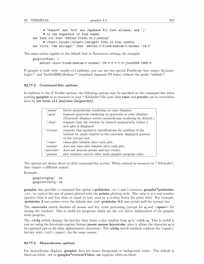
82 TERMINAL gnuplot 4.3 207
# ’kana14’ and ’k14’ are Japanese X11 font aliases, and ’;’# is the separator of font names.
set term x11 font ’mbfont:fixed,16,r,medium’# <font>,<size>,<slant>,<weight> form is also usable.
set title ’(mb strings)’ font ’mbfont:*-fixed-medium-r-normal--14-*’
The same syntax applies to the default font in Xresources settings, for example,
gnuplot*font: \mbfont:-misc-fixed-medium-r-normal--14-*-*-*-c-*-jisx0208.1983-0
If gnuplot is built with –enable-x11-mbfonts, you can use two special PostScript font names ’Ryumin-Light-*’ and ’GothicBBB-Medium-*’ (standard Japanese PS fonts) without the prefix "mbfont:".
82.77.2 Command-line options
In addition to the X Toolkit options, the following options may be specified on the command line whenstarting gnuplot or as resources in your ".Xdefaults" file (note that raise and persist can be overriddenlater by set term x11 [no]raise [no]persist):
‘-mono‘ forces monochrome rendering on color displays.‘-gray‘ requests grayscale rendering on grayscale or color displays.
(Grayscale displays receive monochrome rendering by default.)‘-clear‘ requests that the window be cleared momentarily before a
new plot is displayed.‘-tvtwm‘ requests that geometry specifications for position of the
window be made relative to the currently displayed portionof the virtual root.
‘-raise‘ raises plot window after each plot.‘-noraise‘ does not raise plot window after each plot.
‘-noevents‘ does not process mouse and key events.‘-persist‘ plot windows survive after main gnuplot program exits.
The options are shown above in their command-line syntax. When entered as resources in ".Xdefaults",they require a different syntax.
Example:
gnuplot*gray: ongnuplot*ctrlq: on
gnuplot also provides a command line option (-pointsize <v>) and a resource, gnuplot*pointsize:<v>, to control the size of points plotted with the points plotting style. The value v is a real number(greater than 0 and less than or equal to ten) used as a scaling factor for point sizes. For example,-pointsize 2 uses points twice the default size, and -pointsize 0.5 uses points half the normal size.
The -noevents switch disables all mouse and key event processing (except for q and <space> forclosing the window). This is useful for programs which use the x11 driver independent of the gnuplotmain program.
The -ctrlq switch changes the hot-key that closes a plot window from q to <ctrl>q. This is useful isyou are using the keystroke-capture feature pause mouse keystroke, since it allows the character q tobe captured just as all other alphanumeric characters. The -ctrlq switch similarly replaces the <space>hot-key with <ctrl><space> for the same reason.
82.77.3 Monochrome options
For monochrome displays, gnuplot does not honor foreground or background colors. The default isblack-on-white. -rv or gnuplot*reverseVideo: on requests white-on-black.
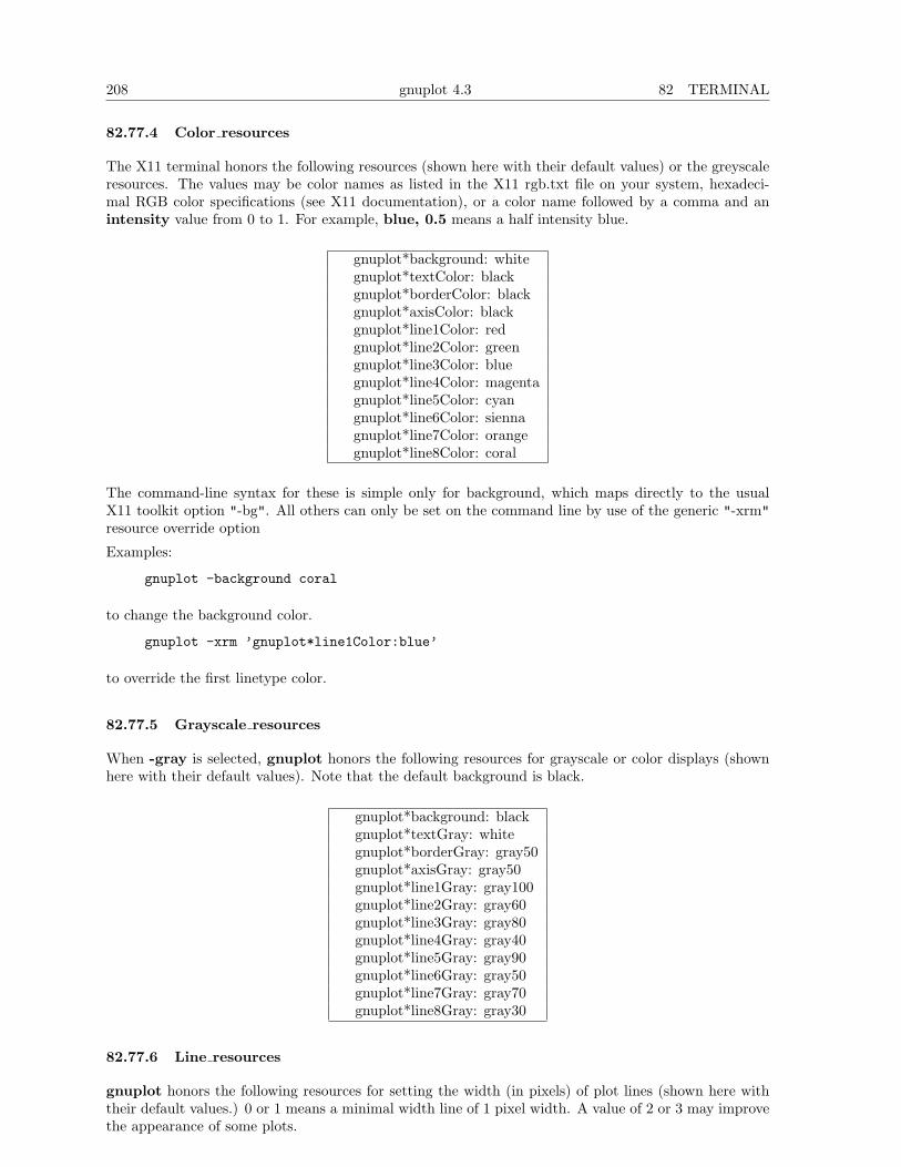
208 gnuplot 4.3 82 TERMINAL
82.77.4 Color resources
The X11 terminal honors the following resources (shown here with their default values) or the greyscaleresources. The values may be color names as listed in the X11 rgb.txt file on your system, hexadeci-mal RGB color specifications (see X11 documentation), or a color name followed by a comma and anintensity value from 0 to 1. For example, blue, 0.5 means a half intensity blue.
gnuplot*background: whitegnuplot*textColor: blackgnuplot*borderColor: blackgnuplot*axisColor: blackgnuplot*line1Color: redgnuplot*line2Color: greengnuplot*line3Color: bluegnuplot*line4Color: magentagnuplot*line5Color: cyangnuplot*line6Color: siennagnuplot*line7Color: orangegnuplot*line8Color: coral
The command-line syntax for these is simple only for background, which maps directly to the usualX11 toolkit option "-bg". All others can only be set on the command line by use of the generic "-xrm"resource override option
Examples:
gnuplot -background coral
to change the background color.
gnuplot -xrm ’gnuplot*line1Color:blue’
to override the first linetype color.
82.77.5 Grayscale resources
When -gray is selected, gnuplot honors the following resources for grayscale or color displays (shownhere with their default values). Note that the default background is black.
gnuplot*background: blackgnuplot*textGray: whitegnuplot*borderGray: gray50gnuplot*axisGray: gray50gnuplot*line1Gray: gray100gnuplot*line2Gray: gray60gnuplot*line3Gray: gray80gnuplot*line4Gray: gray40gnuplot*line5Gray: gray90gnuplot*line6Gray: gray50gnuplot*line7Gray: gray70gnuplot*line8Gray: gray30
82.77.6 Line resources
gnuplot honors the following resources for setting the width (in pixels) of plot lines (shown here withtheir default values.) 0 or 1 means a minimal width line of 1 pixel width. A value of 2 or 3 may improvethe appearance of some plots.
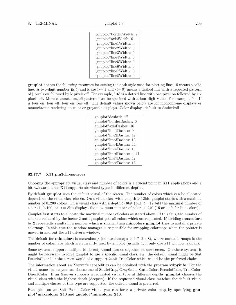
82 TERMINAL gnuplot 4.3 209
gnuplot*borderWidth: 2gnuplot*axisWidth: 0gnuplot*line1Width: 0gnuplot*line2Width: 0gnuplot*line3Width: 0gnuplot*line4Width: 0gnuplot*line5Width: 0gnuplot*line6Width: 0gnuplot*line7Width: 0gnuplot*line8Width: 0
gnuplot honors the following resources for setting the dash style used for plotting lines. 0 means a solidline. A two-digit number jk (j and k are >= 1 and <= 9) means a dashed line with a repeated patternof j pixels on followed by k pixels off. For example, ’16’ is a dotted line with one pixel on followed by sixpixels off. More elaborate on/off patterns can be specified with a four-digit value. For example, ’4441’is four on, four off, four on, one off. The default values shown below are for monochrome displays ormonochrome rendering on color or grayscale displays. Color displays default to dashed:off
gnuplot*dashed: offgnuplot*borderDashes: 0gnuplot*axisDashes: 16gnuplot*line1Dashes: 0gnuplot*line2Dashes: 42gnuplot*line3Dashes: 13gnuplot*line4Dashes: 44gnuplot*line5Dashes: 15gnuplot*line6Dashes: 4441gnuplot*line7Dashes: 42gnuplot*line8Dashes: 13
82.77.7 X11 pm3d resources
Choosing the appropriate visual class and number of colors is a crucial point in X11 applications and abit awkward, since X11 supports six visual types in different depths.
By default gnuplot uses the default visual of the screen. The number of colors which can be allocateddepends on the visual class chosen. On a visual class with a depth > 12bit, gnuplot starts with a maximalnumber of 0x200 colors. On a visual class with a depth > 8bit (but <= 12 bit) the maximal number ofcolors is 0x100, on <= 8bit displays the maximum number of colors is 240 (16 are left for line colors).
Gnuplot first starts to allocate the maximal number of colors as stated above. If this fails, the number ofcolors is reduced by the factor 2 until gnuplot gets all colors which are requested. If dividing maxcolorsby 2 repeatedly results in a number which is smaller than mincolors gnuplot tries to install a privatecolormap. In this case the window manager is responsible for swapping colormaps when the pointer ismoved in and out the x11 driver’s window.
The default for mincolors is maxcolors / (num colormaps > 1 ? 2 : 8), where num colormaps is thenumber of colormaps which are currently used by gnuplot (usually 1, if only one x11 window is open).
Some systems support multiple (different) visual classes together on one screen. On these systems itmight be necessary to force gnuplot to use a specific visual class, e.g. the default visual might be 8bitPseudoColor but the screen would also support 24bit TrueColor which would be the preferred choice.
The information about an Xserver’s capabilities can be obtained with the program xdpyinfo. For thevisual names below you can choose one of StaticGray, GrayScale, StaticColor, PseudoColor, TrueColor,DirectColor. If an Xserver supports a requested visual type at different depths, gnuplot chooses thevisual class with the highest depth (deepest). If the requested visual class matches the default visualand multiple classes of this type are supported, the default visual is preferred.
Example: on an 8bit PseudoColor visual you can force a private color map by specifying gnu-plot*maxcolors: 240 and gnuplot*mincolors: 240.
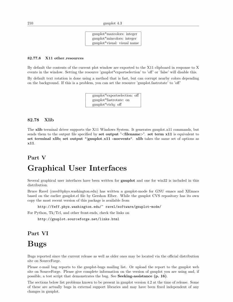
210 gnuplot 4.3
gnuplot*maxcolors: integergnuplot*mincolors: integergnuplot*visual: visual name
82.77.8 X11 other resources
By default the contents of the current plot window are exported to the X11 clipboard in response to Xevents in the window. Setting the resource ’gnuplot*exportselection’ to ’off’ or ’false’ will disable this.
By default text rotation is done using a method that is fast, but can corrupt nearby colors dependingon the background. If this is a problem, you can set the resource ’gnuplot.fastrotate’ to ’off’
gnuplot*exportselection: offgnuplot*fastrotate: ongnuplot*ctrlq: off
82.78 Xlib
The xlib terminal driver supports the X11 Windows System. It generates gnuplot x11 commands, butsends them to the output file specified by set output ’<filename>’. set term x11 is equivalent toset terminal xlib; set output "|gnuplot x11 -noevents". xlib takes the same set of options asx11.
Part V
Graphical User Interfaces
Several graphical user interfaces have been written for gnuplot and one for win32 is included in thisdistribution.
Bruce Ravel ([email protected]) has written a gnuplot-mode for GNU emacs and XEmacsbased on the earlier gnuplot.el file by Gershon Elber. While the gnuplot CVS repository has its owncopy the most recent version of this package is available from
http://feff.phys.washington.edu/~ ravel/software/gnuplot-mode/
For Python, Tk/Tcl, and other front-ends, check the links on
http://gnuplot.sourceforge.net/links.html
Part VI
Bugs
Bugs reported since the current release as well as older ones may be located via the official distributionsite on SourceForge.
Please e-mail bug reports to the gnuplot-bugs mailing list. Or upload the report to the gnuplot website on SourceForge. Please give complete information on the version of gnuplot you are using and, ifpossible, a test script that demonstrates the bug. See Seeking-assistance (p. 16).
The sections below list problems known to be present in gnuplot version 4.2 at the time of release. Someof these are actually bugs in external support libraries and may have been fixed independent of anychanges in gnuplot.
gnuplot 4.3 211
83 Gnuplot limitations
Floating point exceptions (floating point number too large/small, divide by zero, etc.) may occasionallybe generated by user defined functions. Some of the demos in particular may cause numbers to exceedthe floating point range. Whether the system ignores such exceptions (in which case gnuplot labels thecorresponding point as undefined) or aborts gnuplot depends on the compiler/runtime environment.
The gamma and bessel functions do not work for complex arguments.
Only one color palette at a time is active for any given x11 plot window. This means that multiplotswhose constituent plots use different palettes will not display correctly in x11.
Coordinates specified as "time" wrap at 24 hours, and have a precision limited to 1 second. This is inparticular a limitation in using time format to handle geographic coordinates.
Error bars are not handled properly in polar/spherical coordinate plot modes.
The ’nohidden3d’ option that is supposed to exempt individual plots from the global property ’sethidden3d’ does not work for parametric curves.
84 External libraries
External library GD (used by PNG/JPEG/GIF drivers): Versions of libgd through 2.0.33 contain variousbugs in mapping the characters of Adobe’s Symbol font. Also it is possible to trigger a library segfaultif an anti-aliased line crosses an upper corner of the canvas.
External library PDFlib (used by PDF driver): Gnuplot can be linked against libpdf versions 4, 5, or6. However, these versions differ in their handling of piped I/O. Therefore gnuplot scripts using pipedoutput to PDF may work only for some versions of PDFlib.
External library svgalib (used by linux and vgagl driver): Requires gnuplot to be suid root (bad!) andhas many bugs that are specific to the video card or graphics driver used in X11.
Internationalization (locale settings): Gnuplot uses the C runtime library routine setlocale() to controllocale-specific formatting of input and output number, times, and date strings. The locales available,and the level of support for locale features such as "thousands’ grouping separator", depend on theinternationalization support provided by your individual machine.
Part VII
Index
Index
.gnuplot, 34
abs, 24acos, 24acosh, 24acsplines, 72adobeglyphnames, 194aed512, 159aed767, 159aifm, 159amiga, 159angles, 86, 131apollo, 160Aqua, 160aqua, 160arg, 24arrow, 86, 134arrowstyle, 49, 133ascii, 156asin, 24asinh, 24atan, 24atan2, 24atanh, 24automated, 46autoscale, 79, 88avs, 68axes, 20, 29, 33, 64
backquotes, 35bars, 40, 41, 43, 49–51, 77, 78, 90batch/interactive, 15, 18, 54, 62, 85BE, 160be, 160besj0, 24besj1, 24bessel, 211besy0, 24besy1, 24bezier, 72binary, 66, 68, 98, 156binary examples, 69bind, 31, 85, 90, 116bitwise operators, 26bmargin, 90border, 90, 106, 139boxerrorbars, 38, 92boxes, 39, 40, 92boxwidth, 41, 91boxxyerrorbars, 40branch, 59bugs, 210
call, 53, 62candlesticks, 40, 43
canvas, 17, 162cbdata, 151cbdtics, 151cblabel, 152cbmtics, 152cbrange, 29, 30, 123, 125, 136, 153cbtics, 153cd, 52ceil, 24center, 46, 69cgi, 163cgm, 163circle, 18, 41, 120circles, 18, 41clabel, 92, 94, 96, 109clear, 53clip, 49, 92cntrparam, 34, 93, 96, 132, 157color resources, 208colorbox, 30, 94, 123, 125, 153colornames, 29, 30, 95, 136colors, 29, 30, 81, 127, 128, 136colorspec, 30, 112, 119, 136, 137, 141column, 25command line editing, 19command line options, 207command-line-editing, 84command-line-options, 33commands, 52comments, 16, 19, 62commentschars, 19, 98compatibility, 18contour, 34, 52, 92, 94, 95, 106, 137, 138, 157coordinates, 20, 87, 110–112, 119–121, 134, 139,
141, 144, 147copyright, 15corel, 166cos, 24cosh, 24csplines, 72cumulative, 18, 72
data, 48, 64, 96data file, 64datafile, 33, 54, 64, 88, 96, 106, 157datastrings, 20, 48, 80date specifiers, 104debug, 166decimalsign, 17, 98, 101, 103, 113defined, 25degrees, 86depthorder, 51, 124, 126dgrid3d, 18, 99, 132, 138, 157division, 23
212
INDEX gnuplot 4.3 213
dospc, 166dots, 41dpu414, 171dumb, 166dummy, 88, 100dxf, 167dxy800a, 167
edf, 68editing, 19editing postscript, 192eepic, 167egalib, 177egamono, 177ehf, 68ellipse, 18, 120elliptic integrals, 25emf, 168emtex, 180emxvesa, 168emxvga, 168encoding, 17, 21, 101, 113, 177, 187, 190, 204encodings, 101enhanced, 21, 160, 174, 179, 187, 189–191, 197, 201,
204, 205environment, 22epslatex, 169epson 180dpi, 171epson 60dpi, 171epson lx800, 171equal, 133erf, 24erfc, 24error estimates, 56error state, 27, 85errorbars, 65, 77errorlines, 65, 77errors, 27evaluate, 53every, 70example, 70examples, 75excl, 172exists, 25, 35exit, 54exp, 24exponentiation, 26expressions, 23, 82, 105
factorial, 26failsafe, 47fig, 172file, 64fill, 39–41, 44filledcurves, 41fillstyle, 17, 40, 41, 81, 119, 134, 137financebars, 40, 42
fit, 22, 27, 54, 56, 75, 159fit parameters, 55fitting, 56flipx, 46floating point exceptions, 96, 211floor, 24fontfile, 192–194fontpath, 102, 193fonts, 174, 179, 189, 206format, 102, 138, 141, 144, 145, 148format specifiers, 103fortran, 96fpe trap, 96frequency, 72fsteps, 43function, 105functions, 23, 28
gamma, 24, 211gamma correction, 130general, 66, 129, 154, 155ggi, 173gif, 174glossary, 28, 70gnugraph, 175gpbin, 154gpic, 175gpr, 176gprintf, 34, 103, 111graph menu, 201grass, 176grayscale resources, 208grid, 105grid data, 95, 99, 154, 157gui’s, 210guidelines, 57
hcgi, 163help, 60help desk, 16hercules, 177hidden3d, 51, 106, 108histeps, 43histograms, 43history, 61, 84historysize, 107hp2623a, 177hp2648, 177hp500c, 177hpdj, 178hpgl, 177hpljii, 178hppj, 178
ibeta, 24if, 32, 61, 84igamma, 24imag, 24
214 gnuplot 4.3 INDEX
image, 46, 49imagen, 178impulses, 47increment, 136index, 31, 65, 71int, 24internationalization, 211introduction, 15inverf, 24invnorm, 24isosamples, 33, 106, 108, 132, 157iteration, 45, 46, 62, 79, 86, 158
jpeg, 179
kdensity, 18, 73key, 80, 108kyo, 179
label, 47, 111, 116labels, 21, 47, 65, 112, 116lambertw, 24latex, 180lc, 30least squares, 54legend, 108lgamma, 24libgd, 211license, 15line, 30, 87, 95, 134line editing, 19line resources, 208linecolor, 30lines, 48linespoints, 48linestyle, 30, 48, 136linetype, 29, 48, 81linewidth, 48, 136linux, 180lmargin, 113load, 62loadpath, 113, 194locale, 17, 98, 101, 113, 211log, 24, 92log10, 24logscale, 113lower, 62lp, 48lua, 180
macintosh, 181macros, 28, 35, 54map, 52, 125mapping, 114, 131margin, 90, 113, 115, 117, 131, 141Marquardt, 54matrix, 66, 70, 156metafont, 181
metapost, 183mf, 181mgr, 182mif, 182missing, 96mixing macros backquotes, 36modulo, 26monochrome options, 207mouse, 31, 32, 115, 204mp, 183multi branch, 59multi-branch, 55, 59multiplot, 53, 117, 199mx2tics, 118mxtics, 118, 119my2tics, 119mytics, 119mztics, 119
NaN, 23, 28, 75nec cp6, 171negation, 26negative, 127new features, 17newhistogram, 46NeXT, 185next, 185noarrow, 86noautoscale, 88noborder, 90nocbdtics, 151nocbmtics, 152nocbtics, 153noclip, 92nocontour, 95nodgrid3d, 99nofpe trap, 96nogrid, 105nohidden3d, 106, 211nohistorysize, 107nokey, 108nolabel, 111nologscale, 113nomouse, 115nomultiplot, 117nomx2tics, 118nomxtics, 118nomy2tics, 119nomytics, 119nomztics, 119nooffsets, 121noparametric, 122nopolar, 131norm, 24nosurface, 137notimestamp, 140nox2dtics, 143
INDEX gnuplot 4.3 215
nox2mtics, 143nox2tics, 143nox2zeroaxis, 143noxdtics, 144noxmtics, 145noxtics, 146noxzeroaxis, 150noy2dtics, 150noy2mtics, 150noy2tics, 150noy2zeroaxis, 150noydtics, 150noymtics, 151noytics, 151noyzeroaxis, 151nozdtics, 151nozmtics, 152noztics, 152nozzeroaxis, 151
object, 119offsets, 121okidata, 171one’s complement, 26OpenStep, 186Openstep, 186openstep, 186operator precedence, 26operators, 26origin, 53, 117, 121output, 121
palette, 29, 81, 95, 112, 123, 125–127, 136, 137,141, 153
parametric, 88, 122pause, 63pbm, 186pcl5, 177pdf, 186, 211pdfcairo, 187pi, 28placement, 109plot, 63, 64, 84, 153, 154plotting, 33pm, 188pm3d, 51, 87, 95, 123, 125, 134, 137pm3d resources, 209png, 138, 188pngcairo, 190points, 48pointsize, 48, 81, 130polar, 33, 131polygon, 18, 120pop, 138positive, 127postscript, 138, 191, 192practical guidelines, 57
prescribe, 179print, 82printing, 202prologue, 22, 169, 191, 194, 195pseudocolumns, 31, 71, 75, 76pslatex, 170, 194pstex, 194pstricks, 196punctuation, 36push, 138pwd, 83
qms, 196quit, 83quotes, 16, 37
raise, 83, 205rand, 24random, 25range frame, 149rangelimited, 149ranges, 54, 78real, 24rectangle, 119refresh, 17, 64, 74, 83regis, 196replot, 74, 83reread, 61, 84reset, 85, 86restore, 145rgbalpha, 17, 46rgbcolor, 30rgbformulae, 127rgbimage, 46rgip, 197rmargin, 131rotate, 46, 69rrange, 132
samples, 71, 106, 108, 132, 138save, 85sbezier, 72seeking assistance, 16Seeking-assistance, 210separator, 75, 97set, 85sgn, 24shell, 153, 157show, 85sin, 24sinh, 24size, 53, 117, 122, 132skip, 69smooth, 18, 71, 132space, 31special filenames, 73special-filenames, 35specifiers, 103
216 gnuplot 4.3 INDEX
specify, 36splot, 63, 84, 106, 131, 153sprintf, 25, 34, 111sqrt, 24ssvgalib, 177starc, 171start, 34start-up, 22starting values, 59startup, 34statistical overview, 57steps, 49strcol, 25strftime, 25string operators, 26stringcolumn, 25strings, 34, 111strlen, 25strptime, 25strstrt, 25style, 75, 77, 78, 80, 112styles, 81, 133–135substitution, 35, 37, 114substr, 25substring, 25, 34sun, 197surface, 96, 137, 157svg, 197svga, 197svgalib, 177, 211syntax, 16, 36, 103, 109, 141, 145system, 25, 157
table, 138tan, 24tandy 60dpi, 171tanh, 24tc, 30tek40, 198tek410x, 198term, 85, 159terminal, 138, 159termoption, 138ternary, 27test, 81, 158texdraw, 198text, 37, 112, 188text menu, 202textcolor, 30tgif, 198thru, 74tics, 139ticscale, 139ticslevel, 20, 139, 143, 154time specifiers, 104Time/date, 141, 144time/date, 37
timecolumn, 25timefmt, 20, 79, 104, 112, 140, 144, 211timestamp, 140tips, 60title, 21, 108, 141tkcanvas, 199tm hour, 25tm mday, 25tm min, 25tm mon, 25tm sec, 25tm wday, 25tm yday, 25tm year, 25tmargin, 141tpic, 200trange, 141transparency, 47transparent, 135
unary, 26undefine, 158uniplex, 197unique, 72unixpc, 200unixplot, 200unset, 158update, 55, 158urange, 141user defined, 28user-defined, 64using, 21, 27, 38, 55, 74, 77, 78, 123UTF 8, 101, 194
valid, 25variable, 39, 40, 47, 48, 71variables, 27, 28, 31, 33, 56, 63vectors, 49vgagl, 200vgal, 168vgalib, 177vgamono, 177view, 142, 149, 154volatile, 17, 64vrange, 143vttek, 198VWS, 201vx384, 201
wgnuplot.ini, 203windows, 201with, 77, 78, 80, 108, 130, 133, 173word, 25words, 25writeback, 145wxt, 203
X resources, 206–210
INDEX gnuplot 4.3 217
X11, 205x11, 205x11 fonts, 206x11 mouse, 116x2data, 143x2dtics, 143x2label, 143x2mtics, 143x2range, 143x2tics, 143x2zeroaxis, 143xdata, 20, 112, 141, 143, 150, 151xdtics, 143, 144, 150, 151xerrorbars, 49xerrorlines, 50xfig, 172xlabel, 143, 144, 150, 152xlib, 210xmtics, 143, 145, 150–152xrange, 88, 131, 132, 141, 143, 145, 150–153xticlabels, 21, 76, 77xtics, 91, 103, 106, 118, 139, 143, 146, 150–153xyerrorbars, 50xyerrorlines, 51xyplane, 139, 149, 151xzeroaxis, 150
y2data, 150y2dtics, 150y2label, 150y2mtics, 150y2range, 150y2tics, 150y2zeroaxis, 150ydata, 150ydtics, 150yerrorbars, 50yerrorlines, 51ylabel, 150ymtics, 151yrange, 151ytics, 151yzeroaxis, 151
zdata, 151zdtics, 151zero, 151zeroaxis, 143, 149–152zlabel, 152zmtics, 152zrange, 152ztics, 152zzeroaxis, 151