Embed Size (px)
Citation preview

Global Risk Management
Ren-Raw Chen, Ph.D.c© Draft date April 15, 2018

i
Library of Congress Control Number 1234567890Chen, Ren-Raw Global Financial Risk Management – A Quantitative Guide /Ren-Raw ChenISBN 1234567890123
All rights reserved. This book, or parts thereof, may not be reproduced in any formor by any means, electronic or mechanical, including photocopying, recording orany information storage and retrieval system now known or to be invented, withoutwritten permission from the Publisher.

ii

Contents
Contents i
Preface xv
Acknowledgments xvii
I Introduction 1
1 Math Primer 3
1.1 Continuous and Discrete Returns . . . . . . . . . . . . . . . . . . . . 3
1.1.1 Definition . . . . . . . . . . . . . . . . . . . . . . . . . . . . . 3
1.1.2 Average Return . . . . . . . . . . . . . . . . . . . . . . . . . . 4
1.1.3 Annualization and Deannualization . . . . . . . . . . . . . . . 5
1.2 Linear Algebra . . . . . . . . . . . . . . . . . . . . . . . . . . . . . . 5
1.2.1 Addition/subtraction . . . . . . . . . . . . . . . . . . . . . . . 5
1.2.2 Multiplication/Division . . . . . . . . . . . . . . . . . . . . . . 6
1.2.3 Scaling . . . . . . . . . . . . . . . . . . . . . . . . . . . . . . . 6
1.2.4 Power . . . . . . . . . . . . . . . . . . . . . . . . . . . . . . . 6
1.3 Calculus . . . . . . . . . . . . . . . . . . . . . . . . . . . . . . . . . . 7
1.4 Statistics . . . . . . . . . . . . . . . . . . . . . . . . . . . . . . . . . . 8
1.4.1 Random Variable . . . . . . . . . . . . . . . . . . . . . . . . . 8
1.4.2 Stochastic Process . . . . . . . . . . . . . . . . . . . . . . . . 9
1.4.3 dS and ∆S . . . . . . . . . . . . . . . . . . . . . . . . . . . . 9
iii
iv CONTENTS
1.4.4 Normal Distribution . . . . . . . . . . . . . . . . . . . . . . . 9
2 Overview 13
2.1 Introduction . . . . . . . . . . . . . . . . . . . . . . . . . . . . . . . . 13
2.1.1 Business risks versus financial risks . . . . . . . . . . . . . . . 13
2.1.2 Financial risks . . . . . . . . . . . . . . . . . . . . . . . . . . . 14
2.1.3 Ways to measure and manage these risks . . . . . . . . . . . . 17
2.2 Review of Simple Hedging . . . . . . . . . . . . . . . . . . . . . . . . 17
2.3 Market Risk . . . . . . . . . . . . . . . . . . . . . . . . . . . . . . . . 18
2.3.1 Value at Risk . . . . . . . . . . . . . . . . . . . . . . . . . . . 19
2.3.2 Stress Test . . . . . . . . . . . . . . . . . . . . . . . . . . . . . 21
2.4 Credit Risk . . . . . . . . . . . . . . . . . . . . . . . . . . . . . . . . 21
2.4.1 Sources of credit risk . . . . . . . . . . . . . . . . . . . . . . . 22
2.4.2 Credit risk metrics . . . . . . . . . . . . . . . . . . . . . . . . 24
2.5 Liquidity Risk . . . . . . . . . . . . . . . . . . . . . . . . . . . . . . . 25
2.6 Operational Risk (Wiki) . . . . . . . . . . . . . . . . . . . . . . . . . 26
2.7 Risk Management Modeling Building Blocks . . . . . . . . . . . . . . 27
2.7.1 Basic Models by Asset Class . . . . . . . . . . . . . . . . . . . 27
2.7.2 Risk Management Tools available . . . . . . . . . . . . . . . . 28
2.8 Basel Accords . . . . . . . . . . . . . . . . . . . . . . . . . . . . . . . 28
2.8.1 Basel I . . . . . . . . . . . . . . . . . . . . . . . . . . . . . . . 29
2.8.2 Basel II . . . . . . . . . . . . . . . . . . . . . . . . . . . . . . 31
2.8.3 Basel III . . . . . . . . . . . . . . . . . . . . . . . . . . . . . . 33
2.9 Types of Capital . . . . . . . . . . . . . . . . . . . . . . . . . . . . . 34
2.9.1 Regulatory capital . . . . . . . . . . . . . . . . . . . . . . . . 34
2.9.2 Economic capital . . . . . . . . . . . . . . . . . . . . . . . . . 35
2.9.3 Risk-adjusted return on capital (RAROC) . . . . . . . . . . . 35
2.10 Appendix . . . . . . . . . . . . . . . . . . . . . . . . . . . . . . . . . 36
2.10.1 Report on Excite@Homes bankruptcy . . . . . . . . . . . . . . 36

CONTENTS v
3 Hedging 37
3.1 What Is Hedging? . . . . . . . . . . . . . . . . . . . . . . . . . . . . . 37
3.2 Static versus Dynamic Hedging . . . . . . . . . . . . . . . . . . . . . 38
3.2.1 Static Hedging . . . . . . . . . . . . . . . . . . . . . . . . . . 38
3.2.2 Dynamic Hedging . . . . . . . . . . . . . . . . . . . . . . . . . 39
3.2.3 Other Hedging Examples . . . . . . . . . . . . . . . . . . . . . 41
II Market Risk 43
4 Value At Risk 45
4.1 Introduction . . . . . . . . . . . . . . . . . . . . . . . . . . . . . . . . 45
4.1.1 An Example . . . . . . . . . . . . . . . . . . . . . . . . . . . . 47
4.1.2 Limitations of VaR . . . . . . . . . . . . . . . . . . . . . . . . 48
4.1.3 Stress Testing . . . . . . . . . . . . . . . . . . . . . . . . . . . 48
4.1.4 Risk Reporting . . . . . . . . . . . . . . . . . . . . . . . . . . 48
4.1.5 External Disclosure . . . . . . . . . . . . . . . . . . . . . . . . 49
4.1.6 The Basel Accord II . . . . . . . . . . . . . . . . . . . . . . . 49
4.1.7 Capital Regulation . . . . . . . . . . . . . . . . . . . . . . . . 50
4.2 Major Types of VaR . . . . . . . . . . . . . . . . . . . . . . . . . . . 50
4.2.1 Historical VaR . . . . . . . . . . . . . . . . . . . . . . . . . . 52
4.2.2 Parametric VaR . . . . . . . . . . . . . . . . . . . . . . . . . 59
4.2.3 Factor Model Based VaR . . . . . . . . . . . . . . . . . . . . . 64
4.3 Marginal and Component VaR . . . . . . . . . . . . . . . . . . . . . . 73
4.4 Decay . . . . . . . . . . . . . . . . . . . . . . . . . . . . . . . . . . . 75
4.5 Exercises . . . . . . . . . . . . . . . . . . . . . . . . . . . . . . . . . . 76
5 Fixed Income Risk Management 79
5.1 Interest Rates . . . . . . . . . . . . . . . . . . . . . . . . . . . . . . . 79
5.1.1 US Treasuries . . . . . . . . . . . . . . . . . . . . . . . . . . . 79
5.1.2 LIBOR (London Interbank Offer Rate) . . . . . . . . . . . . . 81

vi CONTENTS
5.1.3 Agencies . . . . . . . . . . . . . . . . . . . . . . . . . . . . . . 81
5.1.4 The Model . . . . . . . . . . . . . . . . . . . . . . . . . . . . . 82
5.2 Forward Expectation . . . . . . . . . . . . . . . . . . . . . . . . . . . 91
5.2.1 A Simple Concept . . . . . . . . . . . . . . . . . . . . . . . . . 91
5.2.2 More Formal Mathematics . . . . . . . . . . . . . . . . . . . . 92
5.3 IR Risk Management . . . . . . . . . . . . . . . . . . . . . . . . . . . 93
5.3.1 Conventions . . . . . . . . . . . . . . . . . . . . . . . . . . . . 93
5.3.2 Duration (delta) and Convexity (gamma) . . . . . . . . . . . . 96
5.3.3 IR Swaps . . . . . . . . . . . . . . . . . . . . . . . . . . . . . 99
5.4 FX Risk Management . . . . . . . . . . . . . . . . . . . . . . . . . . 102
5.4.1 FX Forward and Interest Rate Parity . . . . . . . . . . . . . . 102
5.4.2 FX Swaps . . . . . . . . . . . . . . . . . . . . . . . . . . . . . 104
5.4.3 Quanto . . . . . . . . . . . . . . . . . . . . . . . . . . . . . . 110
5.4.4 FX Option Formula . . . . . . . . . . . . . . . . . . . . . . . . 110
5.4.5 FX Basis . . . . . . . . . . . . . . . . . . . . . . . . . . . . . . 111
5.4.6 FX models . . . . . . . . . . . . . . . . . . . . . . . . . . . . . 111
5.5 Total Return Swap . . . . . . . . . . . . . . . . . . . . . . . . . . . . 113
5.6 Residential Mortgage . . . . . . . . . . . . . . . . . . . . . . . . . . . 113
5.6.1 Refinance Modeling . . . . . . . . . . . . . . . . . . . . . . . . 114
5.6.2 Prepayment Modeling . . . . . . . . . . . . . . . . . . . . . . 114
5.6.3 Default Modeling . . . . . . . . . . . . . . . . . . . . . . . . . 116
5.6.4 OAS – Option Adjusted Spread . . . . . . . . . . . . . . . . . 117
5.7 Combined with Other Assets . . . . . . . . . . . . . . . . . . . . . . . 117
5.8 Appendix . . . . . . . . . . . . . . . . . . . . . . . . . . . . . . . . . 118
5.8.1 FX Swap Curve and Fixed-Fixed FX Swaps . . . . . . . . . . 118
5.8.2 Commodities and Real Assets . . . . . . . . . . . . . . . . . . 119
6 P&L Attribution 125
6.1 Introduction . . . . . . . . . . . . . . . . . . . . . . . . . . . . . . . . 125
6.2 Taylor’s Series Expansion and Explanatory Risk Factors . . . . . . . 125

CONTENTS vii
6.3 Pictorial P&L Attribution . . . . . . . . . . . . . . . . . . . . . . . . 127
7 Value Adjustment 129
7.1 VA – Value Adjustment . . . . . . . . . . . . . . . . . . . . . . . . . 129
8 Parameter Estimation 131
8.1 Introduction . . . . . . . . . . . . . . . . . . . . . . . . . . . . . . . . 131
8.2 Regression estimation for the Vasicek model . . . . . . . . . . . . . . 131
8.3 The Cox-Ingersoll-Ross Model . . . . . . . . . . . . . . . . . . . . . . 135
8.4 The Ho-Lee Model . . . . . . . . . . . . . . . . . . . . . . . . . . . . 136
8.5 More sophisticated econometric methods . . . . . . . . . . . . . . . . 138
9 Simulation 139
9.1 Introduction . . . . . . . . . . . . . . . . . . . . . . . . . . . . . . . . 139
9.2 Random Numbers . . . . . . . . . . . . . . . . . . . . . . . . . . . . . 139
9.2.1 Normal/log Normal . . . . . . . . . . . . . . . . . . . . . . . . 139
9.2.2 Poisson . . . . . . . . . . . . . . . . . . . . . . . . . . . . . . 140
9.2.3 Non-central Chi-square . . . . . . . . . . . . . . . . . . . . . . 140
9.2.4 Multi-variate Gaussian . . . . . . . . . . . . . . . . . . . . . . 142
9.3 Examples . . . . . . . . . . . . . . . . . . . . . . . . . . . . . . . . . 144
9.3.1 Black-Scholes . . . . . . . . . . . . . . . . . . . . . . . . . . . 144
9.3.2 Two stocks . . . . . . . . . . . . . . . . . . . . . . . . . . . . 146
9.3.3 Stock with random interest rates . . . . . . . . . . . . . . . . 147
9.4 Homework . . . . . . . . . . . . . . . . . . . . . . . . . . . . . . . . . 149
9.5 Appendix . . . . . . . . . . . . . . . . . . . . . . . . . . . . . . . . . 149
10 Volatility and Extreme Value Theorem 151
10.1 Introduction . . . . . . . . . . . . . . . . . . . . . . . . . . . . . . . . 151
10.2 Implied Volatility and Risk-Neutral Density . . . . . . . . . . . . . . 152
10.3 GARCH . . . . . . . . . . . . . . . . . . . . . . . . . . . . . . . . . . 153
10.4 EWMA . . . . . . . . . . . . . . . . . . . . . . . . . . . . . . . . . . 153
viii CONTENTS
10.5 Extreme Value Theory (EVT) . . . . . . . . . . . . . . . . . . . . . . 154
10.5.1 Estimating Tails of Distributions . . . . . . . . . . . . . . . . 156
10.5.2 Estimating VaR . . . . . . . . . . . . . . . . . . . . . . . . . . 156
10.5.3 Estimating ES . . . . . . . . . . . . . . . . . . . . . . . . . . 157
11 Model Risk 159
11.1 Introduction . . . . . . . . . . . . . . . . . . . . . . . . . . . . . . . . 159
III Credit Risk 161
12 Introduction 163
12.1 Sources of Credit Risk . . . . . . . . . . . . . . . . . . . . . . . . . . 163
12.2 Types of Credit . . . . . . . . . . . . . . . . . . . . . . . . . . . . . . 164
12.2.1 Corporates . . . . . . . . . . . . . . . . . . . . . . . . . . . . . 164
12.2.2 Sovereigns ($ denominated) . . . . . . . . . . . . . . . . . . . 166
12.2.3 Munis . . . . . . . . . . . . . . . . . . . . . . . . . . . . . . . 167
12.2.4 Commercial Mortgages . . . . . . . . . . . . . . . . . . . . . . 168
12.2.5 Retail Credit . . . . . . . . . . . . . . . . . . . . . . . . . . . 168
12.3 Economic Default and Liquidity Default . . . . . . . . . . . . . . . . 170
12.4 Liquidation Process . . . . . . . . . . . . . . . . . . . . . . . . . . . . 170
12.5 Recovery (or Severity) and Loss Given Default (LGD) . . . . . . . . . 170
12.6 Probability of Default (PD) . . . . . . . . . . . . . . . . . . . . . . . 170
13 Reduced-Form Models 173
13.1 Introduction . . . . . . . . . . . . . . . . . . . . . . . . . . . . . . . . 173
13.2 Survival Probability . . . . . . . . . . . . . . . . . . . . . . . . . . . . 173
13.3 Zero Recovery Risky Bond . . . . . . . . . . . . . . . . . . . . . . . . 175
13.3.1 Risky Discount Factor . . . . . . . . . . . . . . . . . . . . . . 175
13.3.2 Zero Recovery Risky Bond . . . . . . . . . . . . . . . . . . . . 175
13.4 Positive Recovery Risky Bond . . . . . . . . . . . . . . . . . . . . . . 175

CONTENTS ix
13.4.1 Recovery of Face Value – The Jarrow-Turnbull Model . . . . . 176
13.4.2 Recovery of Market Value – The Duffie-Singleton Model . . . 177
13.5 Credit Default Swap . . . . . . . . . . . . . . . . . . . . . . . . . . . 180
13.6 Restructuring Definitions by ISDA . . . . . . . . . . . . . . . . . . . 182
13.7 Why Has the CDS Market Developed So Rapidly? . . . . . . . . . . . 183
13.8 Relationship between Default Probabilities and CDS Spreads – Useof the Jarrow-Turnbull Model . . . . . . . . . . . . . . . . . . . . . . 184
13.9 Back-of-the-envelope Formula . . . . . . . . . . . . . . . . . . . . . . 185
13.10Bootstrapping (Curve Cooking) . . . . . . . . . . . . . . . . . . . . . 186
13.11Poisson Assumption . . . . . . . . . . . . . . . . . . . . . . . . . . . . 186
13.12Simple Demonstration (annual frequency) . . . . . . . . . . . . . . . 186
13.13In Reality (quarterly frequency) . . . . . . . . . . . . . . . . . . . . . 191
14 Corporate Finance Approach of Modeling Default 193
14.1 Merton Model . . . . . . . . . . . . . . . . . . . . . . . . . . . . . . . 193
14.2 KMV Model . . . . . . . . . . . . . . . . . . . . . . . . . . . . . . . . 196
14.3 The Geske Model . . . . . . . . . . . . . . . . . . . . . . . . . . . . . 197
14.4 The Leland-Toft Model . . . . . . . . . . . . . . . . . . . . . . . . . . 203
14.5 Hybrid Models . . . . . . . . . . . . . . . . . . . . . . . . . . . . . . 204
15 Credit Portfolio and Credit Correlation 209
15.1 Introduction . . . . . . . . . . . . . . . . . . . . . . . . . . . . . . . . 209
15.2 Basics . . . . . . . . . . . . . . . . . . . . . . . . . . . . . . . . . . . 210
15.3 Default Baskets (First to default) . . . . . . . . . . . . . . . . . . . . 213
15.4 Copula and CDO Pricing . . . . . . . . . . . . . . . . . . . . . . . . . 215
15.4.1 Background . . . . . . . . . . . . . . . . . . . . . . . . . . . . 215
15.4.2 Basics . . . . . . . . . . . . . . . . . . . . . . . . . . . . . . . 216
15.4.3 Factor Copula . . . . . . . . . . . . . . . . . . . . . . . . . . . 218
15.4.4 The Vasicek Model . . . . . . . . . . . . . . . . . . . . . . . . 219
15.4.5 Fourier Inversion and Recursive Algorithm . . . . . . . . . . . 220
15.4.6 An Example . . . . . . . . . . . . . . . . . . . . . . . . . . . . 220
x CONTENTS
15.5 Monte Carlo Simulations . . . . . . . . . . . . . . . . . . . . . . . . . 222
15.5.1 Default Basket . . . . . . . . . . . . . . . . . . . . . . . . . . 222
15.5.2 CDO . . . . . . . . . . . . . . . . . . . . . . . . . . . . . . . . 224
16 Risk Management for Credit Risk 225
16.1 Introduction . . . . . . . . . . . . . . . . . . . . . . . . . . . . . . . . 225
16.2 Unexpected Loss . . . . . . . . . . . . . . . . . . . . . . . . . . . . . 225
16.3 Term Structure of Credit VaR . . . . . . . . . . . . . . . . . . . . . . 226
16.4 CVA – Credit Value Adjustment . . . . . . . . . . . . . . . . . . . . . 227
16.4.1 Exposure . . . . . . . . . . . . . . . . . . . . . . . . . . . . . 229
16.4.2 CCDS (contingent credit default swap) . . . . . . . . . . . . . 233
16.4.3 CVA Hedging . . . . . . . . . . . . . . . . . . . . . . . . . . . 234
16.4.4 CSA (credit support annex) . . . . . . . . . . . . . . . . . . . 234
16.4.5 Counterparty Credit Risk (CCR) as Market Risk . . . . . . . 236
16.4.6 Counterparty Credit Risk (CCR) as Credit Risk . . . . . . . . 237
16.4.7 Counterparty Credit Risk (CCR) Capital under Basel II & III 237
16.4.8 CVA Capital Charge and Basel III . . . . . . . . . . . . . . . 237
16.4.9 Advanced CVA Capital Charge . . . . . . . . . . . . . . . . . 238
16.5 Risky Funding . . . . . . . . . . . . . . . . . . . . . . . . . . . . . . . 239
16.6 Appendix . . . . . . . . . . . . . . . . . . . . . . . . . . . . . . . . . 240
16.6.1 Poisson Process of Defaults . . . . . . . . . . . . . . . . . . . 240
16.6.2 Equation 13.23 . . . . . . . . . . . . . . . . . . . . . . . . . . 243
IV Liquidity Risk 245
17 Liquidity Quantification 247
17.1 Introduction . . . . . . . . . . . . . . . . . . . . . . . . . . . . . . . . 247
17.1.1 Some Liquidity Squeeze Examples . . . . . . . . . . . . . . . . 248
17.2 Understanding Liquidity and Liquidity Risk . . . . . . . . . . . . . . 249
17.3 How to Measure Liquidity . . . . . . . . . . . . . . . . . . . . . . . . 249

CONTENTS xi
17.4 Liquidity and Liquidity Risk . . . . . . . . . . . . . . . . . . . . . . . 250
17.5 How to Measure Liquidity Risk . . . . . . . . . . . . . . . . . . . . . 251
17.5.1 Liquidity Discount as a Put Option . . . . . . . . . . . . . . . 251
17.5.2 The Model . . . . . . . . . . . . . . . . . . . . . . . . . . . . . 254
17.6 Some Analysis . . . . . . . . . . . . . . . . . . . . . . . . . . . . . . . 259
17.7 Liquidity Premium . . . . . . . . . . . . . . . . . . . . . . . . . . . . 269
18 Funding Value Adjustment 273
18.1 FVA in a Netshell . . . . . . . . . . . . . . . . . . . . . . . . . . . . . 273
18.1.1 What is FVA? . . . . . . . . . . . . . . . . . . . . . . . . . . . 273
18.1.2 FVA for Collateralized Trades . . . . . . . . . . . . . . . . . . 273
18.1.3 FVA for Collateralized Trades . . . . . . . . . . . . . . . . . . 275
18.1.4 Conclusion . . . . . . . . . . . . . . . . . . . . . . . . . . . . . 275
18.2 Modeling Risky Funding . . . . . . . . . . . . . . . . . . . . . . . . . 276
18.3 Notation and basic layout . . . . . . . . . . . . . . . . . . . . . . . . 277
18.4 Valuation of bullet loans . . . . . . . . . . . . . . . . . . . . . . . . . 279
18.4.1 The deal leg of a bullet loan . . . . . . . . . . . . . . . . . . . 279
18.4.2 The funding leg of a bullet loan . . . . . . . . . . . . . . . . . 280
18.4.3 An example when default times are independent . . . . . . . . 283
18.4.4 An example when default times are correlated . . . . . . . . . 285
18.5 Valuation of a general derivative contract . . . . . . . . . . . . . . . . 286
18.5.1 Valuation of the deal leg . . . . . . . . . . . . . . . . . . . . . 286
18.5.2 Valuation of the funding leg . . . . . . . . . . . . . . . . . . . 287
18.6 Liquidity . . . . . . . . . . . . . . . . . . . . . . . . . . . . . . . . . . 288
18.7 Summary and Future Research . . . . . . . . . . . . . . . . . . . . . 290
18.8 Collateral Management . . . . . . . . . . . . . . . . . . . . . . . . . . 290
18.9 Appendix . . . . . . . . . . . . . . . . . . . . . . . . . . . . . . . . . 292
18.9.1 Proof of Theorem 1 . . . . . . . . . . . . . . . . . . . . . . . . 292
18.9.2 Proof of Theorem 2 . . . . . . . . . . . . . . . . . . . . . . . . 293

xii CONTENTS
19 A Story about the Financial Crisis – A Case Study of LehmanBrothers 297
19.1 Introduction . . . . . . . . . . . . . . . . . . . . . . . . . . . . . . . . 297
19.2 Richard (Dick) Fuld . . . . . . . . . . . . . . . . . . . . . . . . . . . 298
19.3 Lehman Time Line . . . . . . . . . . . . . . . . . . . . . . . . . . . . 298
19.4 Lehman Default Probability . . . . . . . . . . . . . . . . . . . . . . . 301
19.5 Lehman Liquidity Problems . . . . . . . . . . . . . . . . . . . . . . . 304
19.6 Appendix . . . . . . . . . . . . . . . . . . . . . . . . . . . . . . . . . 304
19.6.1 Lehman Timeline . . . . . . . . . . . . . . . . . . . . . . . . . 304
V Others 309
20 Operational Risk Management 311
20.1 Introduction . . . . . . . . . . . . . . . . . . . . . . . . . . . . . . . . 311
20.2 Basel II event type categories . . . . . . . . . . . . . . . . . . . . . . 311
20.3 Methods of Operational Risk Management . . . . . . . . . . . . . . . 312
20.3.1 Basic Indicator Approach . . . . . . . . . . . . . . . . . . . . 313
20.3.2 Standardized Approach . . . . . . . . . . . . . . . . . . . . . . 313
20.3.3 Internal Measurement Approach . . . . . . . . . . . . . . . . . 315
21 Types of Capital 321
21.1 Introduction . . . . . . . . . . . . . . . . . . . . . . . . . . . . . . . . 321
21.2 Regulatory Capital (wiki) . . . . . . . . . . . . . . . . . . . . . . . . 321
21.2.1 Tier 1 capital . . . . . . . . . . . . . . . . . . . . . . . . . . . 321
21.2.2 Tier 2 (supplementary) capital . . . . . . . . . . . . . . . . . . 322
21.2.3 Common capital ratios . . . . . . . . . . . . . . . . . . . . . . 323
21.2.4 Capital adequacy ratio . . . . . . . . . . . . . . . . . . . . . . 323
21.3 Economic Capital (Wiki) . . . . . . . . . . . . . . . . . . . . . . . . . 326
21.3.1 E&Y Model . . . . . . . . . . . . . . . . . . . . . . . . . . . . 326
21.4 Risk Adjusted Return On Capital (RAROC) . . . . . . . . . . . . . . 331

CONTENTS xiii
21.4.1 Basic formula . . . . . . . . . . . . . . . . . . . . . . . . . . . 331
21.5 David Chow . . . . . . . . . . . . . . . . . . . . . . . . . . . . . . . . 332
21.5.1 Gap Analysis . . . . . . . . . . . . . . . . . . . . . . . . . . . 332
22 Stress Testing, DFAST, CCAR, and CVaR 333
22.1 Introduction . . . . . . . . . . . . . . . . . . . . . . . . . . . . . . . . 333
22.2 Stress Testing . . . . . . . . . . . . . . . . . . . . . . . . . . . . . . . 333
22.2.1 Historical Stress Testing . . . . . . . . . . . . . . . . . . . . . 333
22.2.2 Parametric Stress Testing . . . . . . . . . . . . . . . . . . . . 334
22.2.3 Conditional Stress Testing . . . . . . . . . . . . . . . . . . . . 334
22.2.4 Reverse Stress Testing . . . . . . . . . . . . . . . . . . . . . . 334
22.2.5 A Simple Demonstration . . . . . . . . . . . . . . . . . . . . . 335
22.3 Comprehensive Capital Analysis and Review (CCAR) . . . . . . . . . 336
22.4 Dodd-Frank Act Stress Testing (DFAST) . . . . . . . . . . . . . . . . 337
22.5 Credit VaR . . . . . . . . . . . . . . . . . . . . . . . . . . . . . . . . 338
Index 339

xiv CONTENTS

Preface
I have done risk management research for more than two decades. In fact, my firstindustry work was at JP Morgan (15 Broad Street – the legendary building) inFebruary of 1992 when Mr. Paul Morrison hired me to validate models used by JPMorgan at the time. Since then I had been mostly in the front office (including1997 ∼ 1999 at Lehman as the desk quant in the Structured Credit Desk where Mr.Ken Ulmazaki was the head). In January of 2005, I joined Morgan Stanley ModelReview Group and have been back on risk management till now.
In the summer of 2012, I was asked to teach this course for a group of talentedEMBA students from the Peking University (our first MSGF program) and I havebeen gradually collecting my past notes. That is how this book came to existence.I am extremely grateful to all the past students who took this course from meand hence discovered the numerous mistakes in the original drafts. I particularlywould like to thank the 2014 MSGF and 2015 MSQF classes who had made valuablesuggestions and corrections to this book.
Ren-Raw Chen
New York, New York, April, 2016
xv

xvi CONTENTS

Acknowledgments
I first need to thank my wife, Hsing-Yao, for her support for all these years. Withouther taking care of all the work at home, I would not have achieved not only thisbook, but any of my research. Her unconditional love and support is the main reasonI could accomplish anything at all.
I must thank Dr. Phelim Boyle and Dr. Louis Scott for their caring and sup-port for all these years. Without their patience, encouragement, and kind guidance,this book would never be possible.
As mentioned in Preface, former students from MSQF and MSGF have helpedin many tremendous ways in improving coverage, substances, and accuracy in thisbook. In particular, I would like to thank Yingqi Tian and Zhifang Sun (2015MSQF) who have discovered important mistakes in earlier manuscripts.
xvii

Part I
Introduction


Chapter 1
Math Primer
1.1 Continuous and Discrete Returns
It is quite conventional (almost universal) to use returns to measure the performance(and risks) of a financial investment. Yet, no consensus has been reached on howthey are calculated.
1.1.1 Definition
A discrete return is defined as:
rt =Pt+1 − Pt
Pt(1.1)
where P is price of an asset and t is time. Pt+1 and Pt are two consecutive prices(could be daily, weekly, monthly, etc.)
A continuous return is defined as:
rt = lnPt+1
Pt= lnPt+1 − lnPt (1.2)
The two returns are very close to each other when the prices are observedfrequently (e.g. daily) and start to deviate from each other over low frequencies(e.g. annually). Note that if the two consecutive dates are close to each other, likedaily, then equation (1.1) can be approximated as dP/P which is identical to d lnP ,which is the definition of the continuous return by equation (1.2).
For example, we take the FaceBook stock:

4 Chapter 1: Math Primer
FB ReturnsDate Price Disc. Cont.
12/23/2008 26.9312/25/2008 26.51 -0.0156 -0.015712/26/2008 26.05 -0.0174 -0.017512/27/2008 25.91 -0.0054 -0.005412/30/2008 26.62 0.0274 0.0270
1.1.2 Average Return
It is common that we take average returns. We often compute returns of a certainfrequency (e.g. daily) and store them in a database. Then we compute an averagereturn over a particular time horizon (e.g. one year). In such a case, we need toknow how an average is taken. There are two ways of “taking an average:
• geometrically and
• arithmetically
Theoretically, a geometric average is matched with discrete returns and anarithmetic average is matched with continuous returns, as demonstrated in the fol-lowing equations:
r = n
√(Pt+1
Pt
)(Pt+2
Pt+1
)· · ·(
Pt+nPt+(n−1)
)− 1
= n
√(Pt+nPt
)− 1
and
r =ln(Pt+1
Pt
)+ ln
(Pt+2
Pt+1
)· · ·+ ln
(Pt+n
Pt+(n−1)
)n
=1
nln
(Pt+nPt
)In terms of FB, the average discrete return is 4
√26.62/26.51 − 1 = −0.00289
and the average continuous return is ln[26.62/26.51]/4 = 0.002289. We see that thetwo averages are so close to each other (indistinguishable at the 6th decimal place).

Linear Algebra 5
1.1.3 Annualization and Deannualization
Usually returns are reported in a per annum term, known as annualization. Forexample, The daily return of FB between 12/26/2008 and 12/27/2008 is −0.0054.This one-day return needs to be “annualized” into a per annum return. Given thatthere are approximately 252 trading days in a year, this number is multiplied by252 to be −1.36 or −136%.
Reverse (deannualization) is used sometimes when we need raw returns. Forexample a 3-month return of 12% really is 3% for three months. Since someone elsedid the annualization, you must reverse it to get the raw return for the 3 months.
Standard deviations are annualized and deannualized as well. Instead of mul-tiplying (and dividing) by the same adjustment factor (e.g. 252 for daily), it ismultiplied by the square root of the factor (e.g.
√252). In other words, 1% daily
standard deviation is translated into 15.87% per annum standard deviation.
1.2 Linear Algebra
Matrix operations are important in performing calculations for risk management, aswe are dealing with portfolios of large numbers of assets. Furthermore, MicrosoftExcel now is equipped with matrix operation functions (via Ctrl-Shft-Enter as op-posed to Enter) that can be easily matched with mathematical expressions. As aresult, using matrices is extremely convenient and efficient.
Throughout this book, a matrix is symbolized as a bold non-italic letter. Usu-ally a subscript is given as the dimension (row by column) of the matrix. Formally,we define Am×n as an m-row, n-column rectangular matrix. For example,
[ ]2×3
is a matrix with 2 rows and 3 columns.
1.2.1 Addition/subtraction
Two matrices can be summed or subtracted only if they have identical dimensions.

6 Chapter 1: Math Primer
1.2.2 Multiplication/Division
Two matrices can be multiplied only if the second subscript (i.e. column) of thefirst matrix matches with the first subscript (i.e. row) of the second matrix.
3×2
[ ]2×4
=
3×4
and the resulting matrix has the dimension of the first subscript of the firstmatrix (row) and the second subscript of the second matrix, as the example aboveshows.
The rule of multiplication is the ith row of the first matrix “sumproduct” bythe jth column of the second matrix, as demonstrated below:
1 2 1 3 5 7 5 11 17 23
3 4 2 4 6 8 11 25 39 53
6 5 16 38 60 82
=××××
Figure 1.1: Matrix Multiplication
5 = 1× 1 + 2× 2.
Divisions are performed via matrix inversion. In other words, Am×n ÷ B =Am×n ×B−1. Given that only square matrices can be inversed, matrix Bn×n mustbe n rows and n columns.
1.2.3 Scaling
Any matrix can be scaled up or down by multiplying by a real number. When amatrix is multiplied by a real number, it is identical to each element of the matrixbeing multiplied by the real number.
1.2.4 Power
Matrices can be taken to a power, just like any real number. However, unlikescaling, it is NOT equal to each element raising to the power. Since, we do not usethis function often, we choose to ignore it.

Calculus 7
1.3 Calculus
Sensitivities of prices relative to risk factors are defined as partial derivatives. P&Lanalyses are leveraged upon total derivatives. As a result, some basic knowledge ofcalculus is helpful in understanding risk.
Under a single variable, partial derivatives are the same as total derivatives,as shown below:
y = f(x) = 3x2 + 2x+ 5
y′ =dy
dx= 6x+ 2
With two variables such as:
z = f(x, y) = 3x3 + 6y2 + 4x+ 2y + 5
partial derivatives and total derivatives are not the same. The partials (∂) are:
∂z
∂x= 9x+ 4
∂z
∂y= 12y + 2
The total derivative of z is (via Taylor’s series expansion):
dz =∂z
∂xdx+
∂z
∂ydy
In order to see the impact from x and y changes, we can divide dz by dx ordy, as follows:
dz
dx=∂z
∂x+∂z
∂y
dy
dx= 9x+ 4 + (12y + 2)
dy
dxdz
dy=∂z
∂x
dx
dy+∂z
∂y= (9x+ 4)
dx
dy+ (12y + 2)
where we can see the interaction between x and y. If x and y are unrelated (dx/dy =0 and vice versa), then totals equal partials.
Partial derivatives measure sensitivities of the price a financial asset (z) withrespective to risk factors (x and y). That is, how much is the price movement if one

8 Chapter 1: Math Primer
risk factor moves by a little while all else factors are held constant (usually 1 basispoint, known as DV01 or PV01).
Total derivatives measure price movements when all risk factors are consid-ered. As shown above, it needs the result of partial derivatives (i.e. Taylor’s seriesexpansion). Both risk factors (x and y) move by a little (1 basis point) and togetheris the total impact of price movement. Now we can regard dz and price change. Inrisk management, we try to explain why and how a price is moved up or down (i.e.price change).
Either total derivatives or partial derivatives measure sensitivities of the in-terested variable (i.e. P&L) with respect to risk factors. In other words, either dor ∂ represents a small change. In reality, as analytical derivatives (as those shownabove) do not exist, numerical derivatives are a must. For the sake of convenience,d or ∂ is often replaced by ∆. For example ∆P represents the price change.
1.4 Statistics
Statistics are a crucial tool in modeling risk. As we shall see, the most commonway to view risk is an asset’s price fluctuation. And the easiest way to modelprice fluctuation is the standard deviation of the price (or more precisely return)distribution. A very common choice of the distribution is the normal (i.e. Gaussian)distribution which is bell-shaped, symmetrical, and no upper or lower limits.
1.4.1 Random Variable
A distribution is applied to a “random variable” because a random variable is avariable that we do not know its value. Hence, a set of (possible) values are assigned,which form a distribution. In other words, a distribution is a collection of all possiblevalues of a random variable.
Usually we represent the price of a financial asset as a random variable as wedo not know its value in the future. For example, we do not know the price of theIBM a week from now. Hence, we collect all possible values of the price and forma distribution. Usually we say that the possible prices follow a normal (Gaussian)distribution.

Statistics 9
1.4.2 Stochastic Process
A stochastic process is a collection of the same random variables over time. Forexample, weekly future IBM stock prices form a stochastic process.
dS
S= µdt+ σdW
where dW ∼ N(0, dt). If dt is a week, then it is equal to 1/52 ∼ 0.019230769. Thismeans that the weekly return of a stock is normally distributed with mean µ × dtand variance σ2 × dt.
We shall see that this particular model (known as the Black-Scholes model)has no knowledge of time (known as stationarity). That is, all weekly returns of thestock no matter when have the same expected value and variance. While we canregard dW just as a normal random variable, we shall note that W is named afterNorbert Wiener.1
1.4.3 dS and ∆S
Sometimes, we use ∆S for price change, as opposed to dS.
Sometimes, we just use ∆ for price change.
1.4.4 Normal Distribution
Normal (Gaussian) distribution is used dominantly. Hence it is essential that onecan obtain normal probabilities quickly. One method is to use the lookup tablewhich is embedded in many investments texts.
The table only runs to the second digit for the critical value. To obtaina probability of, say, 1.2524, one usually uses a linear interpolation to approxi-mate. Since 1.2524 is in between 1.25 and 1.26, we just take a weighted aver-age of the two. N(1.25) = 0.8944 and N(1.26) = 0.8962. Hence, N(1.2524) =(76%) × 0.8944 + (24%) × 0.8962 = 0.8948. The other is to use the Excel functionNormSDist(x) where x is the critical value in the Normal distribution. For exampleNormSDist(1.2524) = 0.89478786.
The table usually presents results for only positive x. This is because Normalis symmetrical and any negative x value can be flipped to acquire the positive value.
1Norbert Wiener (November 26, 1894 – March 18, 1964) was an American mathematician andphilosopher. He was Professor of Mathematics at MIT.

10 Chapter 1: Math Primer
Normal Probability Table
0.00 0.01 0.02 0.03 0.04 0.05 0.06 0.07 0.08 0.09
0.0 0.5000 0.5040 0.5080 0.5120 0.5160 0.5199 0.5239 0.5279 0.5319 0.5359
0.1 0.5398 0.5438 0.5478 0.5517 0.5557 0.5596 0.5636 0.5675 0.5714 0.5753
0.2 0.5793 0.5832 0.5871 0.5910 0.5948 0.5987 0.6026 0.6064 0.6103 0.6141
0.3 0.6179 0.6217 0.6255 0.6293 0.6331 0.6368 0.6406 0.6443 0.6480 0.6517
0.4 0.6554 0.6591 0.6628 0.6664 0.6700 0.6736 0.6772 0.6808 0.6844 0.6879
0.5 0.6915 0.6950 0.6985 0.7019 0.7054 0.7088 0.7123 0.7157 0.7190 0.7224
0.6 0.7257 0.7291 0.7324 0.7357 0.7389 0.7422 0.7454 0.7486 0.7517 0.7549
0.7 0.7580 0.7611 0.7642 0.7673 0.7704 0.7734 0.7764 0.7794 0.7823 0.7852
0.8 0.7881 0.7910 0.7939 0.7967 0.7995 0.8023 0.8051 0.8078 0.8106 0.8133
0.9 0.8159 0.8186 0.8212 0.8238 0.8264 0.8289 0.8315 0.8340 0.8365 0.8389
1.0 0.8413 0.8438 0.8461 0.8485 0.8508 0.8531 0.8554 0.8577 0.8599 0.8621
1.1 0.8643 0.8665 0.8686 0.8708 0.8729 0.8749 0.8770 0.8790 0.8810 0.8830
1.2 0.8849 0.8869 0.8888 0.8907 0.8925 0.8944 0.8962 0.8980 0.8997 0.9015
1.3 0.9032 0.9049 0.9066 0.9082 0.9099 0.9115 0.9131 0.9147 0.9162 0.9177
1.4 0.9192 0.9207 0.9222 0.9236 0.9251 0.9265 0.9279 0.9292 0.9306 0.9319
1.5 0.9332 0.9345 0.9357 0.9370 0.9382 0.9394 0.9406 0.9418 0.9429 0.9441
1.6 0.9452 0.9463 0.9474 0.9484 0.9495 0.9505 0.9515 0.9525 0.9535 0.9545
1.7 0.9554 0.9564 0.9573 0.9582 0.9591 0.9599 0.9608 0.9616 0.9625 0.9633
1.8 0.9641 0.9649 0.9656 0.9664 0.9671 0.9678 0.9686 0.9693 0.9699 0.9706
1.9 0.9713 0.9719 0.9726 0.9732 0.9738 0.9744 0.9750 0.9756 0.9761 0.9767
2.0 0.9772 0.9778 0.9783 0.9788 0.9793 0.9798 0.9803 0.9808 0.9812 0.9817
2.1 0.9821 0.9826 0.9830 0.9834 0.9838 0.9842 0.9846 0.9850 0.9854 0.9857
2.2 0.9861 0.9864 0.9868 0.9871 0.9875 0.9878 0.9881 0.9884 0.9887 0.9890
2.3 0.9893 0.9896 0.9898 0.9901 0.9904 0.9906 0.9909 0.9911 0.9913 0.9916
2.4 0.9918 0.9920 0.9922 0.9925 0.9927 0.9929 0.9931 0.9932 0.9934 0.9936
2.5 0.9938 0.9940 0.9941 0.9943 0.9945 0.9946 0.9948 0.9949 0.9951 0.9952
2.6 0.9953 0.9955 0.9956 0.9957 0.9959 0.9960 0.9961 0.9962 0.9963 0.9964
2.7 0.9965 0.9966 0.9967 0.9968 0.9969 0.9970 0.9971 0.9972 0.9973 0.9974
2.8 0.9974 0.9975 0.9976 0.9977 0.9977 0.9978 0.9979 0.9979 0.9980 0.9981
2.9 0.9981 0.9982 0.9982 0.9983 0.9984 0.9984 0.9985 0.9985 0.9986 0.9986
3.0 0.9987 0.9987 0.9987 0.9988 0.9988 0.9989 0.9989 0.9989 0.9990 0.9990
Example: N(1.25)=0.8944 and N(-1.25)=1-N(1.25)=0.1056
Figure 1.2: Normal Probability Table

Statistics 11
In other words, N(−x) = 1−N(x). For example, NormSDist(1.64485) is 0.95 andNormSDist(-1.64485) is 1 − 0.95 = 0.05. Excel also provides an inverse functionto obtain the critical value once given the probability – NormSInv(p). For exampleNormSInv(0.05) is −1.64485.
While NormSDist(x) gives the probability of a standard normal (mean 0 andvariance 1), NormDist(µ, σ2, x), on the other hand, gives a normal probability withmean and variance.
Excel also provides various other statistical functions which are very helpful.

12 Chapter 1: Math Primer

Chapter 2
Overview
2.1 Introduction
Risk management is a crucial function in any corporation or business. And itssuccess relies on both scientific tools and human judgments. The former can bestandardized globally yet the latter depends on local cultures which vary from regionto region, religion to religion, and regulation to regulation.
Hence, the focus of this book is on the scientific side of risk management, thepart that can be globalized. Furthermore, while some of the tools introduced inthis book can be applied to all types of companies and businesses, they are mostlyused by financial companies. Examples given in this book are also mostly from thefinancial sector.
2.1.1 Business risks versus financial risks
In general, there are two broad types of risk any company or business faces thebusiness risk (the left-hand-side of the balance sheet) and the financial risk (theright-hand-side of the balance sheet). The business risk refers to the uncertaintyin the investments of the company, i.e. the assets. The financial risk refers tothe uncertainty the debt capacity (in other words, the instability of its financingcapability). For a financial institution, its assets consist of pre-dominantly financialsecurities and hence its business risk is also financial and the tools for managing thefinancial risk apply to managing its assets.
For an industrial company (i.e. non-financial), the business risk and the fi-nancial risk can be quite unrelated. Take Apple Inc. as an example, its assets areall the manufacturing facilities and its top-notch scientists, engineers, and workers.

14 Chapter 2: Overview
Its business risk comes mainly from it can maintain its superiority in the cell phoneand tablet businesses. The way to manage this risk is to keep innovating and beingthe dominant leader in these businesses. Hence the tools of managing the financialrisk have absolutely no connection to how it manages its business risk. In fact, inthe case of Apple Inc., the business risk is so important that it makes the financialrisk entirely trivial.
But history has taught us that financial risk could be crucial for industrialcompanies. In 2001, a company named Excite@Home filed bankruptcy due to itsfailure to fulfill a convertible bond obligation of near $30 million. During the inter-net bubble (late 1990s to early 2000s), many internet companies issued convertiblebonds as a new financial innovative tool to finance their large capital investments.Convertible bonds were popular then because mutual funds and especially pensionfunds can purchase (these companies cannot purchase stocks not listed in S&P 500list of constituents) and benefit from their fast growth. Excite@Home was majorityowned by AT&T (over 30%) and was the sole provider of internet services (combinedwith Comcast) in the tri-state area. It was perceived that Excite@Home to be one ofthe major internet services providers (especially because it was backed by AT&T).Hence, Excite@Homes bankruptcy was strictly a liquidity default (lack of cash) andnot an economic default. In other words, Excite@Home was one typical example ofhow a successful industry company can bankruptcy due to bad management of itsfinancial risk.
While the two sides of a companys risk must both be managed well to guaranteethe companys survival, it has not been possible to integrate these two sides well untilnow. The new concept of enterprise risk has emerged recently that both businessand financial risks are connected and need to be managed in an integrated manner.ERP (Enterprise Resource Planning) as a result becomes a standard for companies tofollow. However, the focus of this book is the tools for financial risk management.Yet, as mentioned above, these tools can also be applied to many aspects of thebusiness risk of the company. In fact, the overlap of the tools is why the reasonERP can be successfully applied in companies.
2.1.2 Financial risks
Financial risks are caused by fluctuations in prices of goods and financial securitiesgenerally called asset classes. The following are common asset classes:
• commodities: which are further categorized into:
• agriculture products such as corn, soy bean, oranges, sugar, cotton, etc.
– metallurgical products such as gold, silver, copper, etc.

Introduction 15
– livestock products such as cattle, lean hogs, pork belly, etc.
– energy products such as oil (various kinds), gas, etc.
• foreign currencies (euro, yen, yuan, etc.)
• equities
• interest rates (Treasuries, LIBOR , OIS , etc.)
• credit
• mortgage-backed securities
While each asset class (and its subclass) has its own risk, these risks are gen-erally group into four major categories, defined by Basel Accords that are the mostsophisticated bank regulation documentation available today. We shall describe thethree Basel Accords later. According to the Accords, financial risk can be catego-rized as:
• Market risk
• Credit risk
• Liquidity risk
• Operational risk
Market risk
Market risk refers to risk that should be monitored and managed on a very frequentbasis (at least daily) because as market conditions change, market prices move andhence profits and losses are generated. As a result, market risk is usually measuredby the degree of fluctuations in prices know as volatility, or in technical termsthe standard deviation of the price change (or return). In other words, the higheris the volatility (standard deviation), the higher is the risk. Market risk exists inevery asset class, but some are easier to monitor than others. For example, equitiesare transacted very frequently (many times a day) so their market risk is easier tocompute and measured. Fixed income securities, such as swaps, are not transactedfrequently and hence the market risk is not easy to compute. As a result, somescientific methods are necessary to estimate the market risk.

16 Chapter 2: Overview
Credit risk
Credit risk refers to losses due to credit events the most severe of which is bankruptcy.Credit default swaps (CDS) are the contract that provide the perfect hedge of thebankruptcy risk. CDS will be fully explored later in this book. In addition to thebankruptcy risk, market participants also transact bonds whose prices are basedupon the probability of bankruptcy (known as credit spreads). As the probabili-ties move up or down, bond prices (or spreads) move up or down as well. Finally,pension funds and selected mutual funds are regulated to only purchase bonds withinvestment grades. Hence, if a bond is downgraded out of the investment group, itwill be dumped in the marketplace immediately and huge losses can occur. This isknown as the migration risk that must be also managed.
Liquidity risk
Liquidity risk refers to losses of asset values due to lack of trading in the marketplace. Usually, lack of trading introduces higher bid/offer spreads. In a severesituation, the market becomes one-sided and offer (or bid) disappears. Then thebid price can skyfall and large liquidity discounts should occur. During the 2008crisis, we witnessed the exact same phenomenon. Banks were dumping subprimeportfolios to the market after they realized that they were too slow in reacting tothe defaults in subprime loans. Lack of buying (one-sided market) caused the pricesof subprime portfolio to skyfall and resulted in the liquidity crisis.
Operational risk
Operational risk refers to losses due to human mistakes or frauds. In early September2011, UBS announced that it had lost 2.3 billion dollars, as a result of unauthorizedtrading performed by Kweku Adoboli, a director of the bank’s Global SyntheticEquities Trading team in London. On 16 April 2008, The Wall Street Journalreleased a controversial article suggesting that some banks might have understatedborrowing costs they reported for the LIBOR during the 2008 credit crunch thatmay have misled others about the financial position of these banks. On 27 July2012, the Financial Times published an article by a former trader which statedthat LIBOR manipulation had been common since at least 1991. LIBOR underpinsapproximately $350 trillion in derivatives. On 27 June 2012, Barclays Bank wasfined $200 million by the Commodity Futures Trading Commission, $160 million bythe United States Department of Justice and 59.5 million by the Financial ServicesAuthority for attempted manipulation of the LIBOR and Euribor rates.

Review of Simple Hedging 17
Collateral risk
Collateral risk is not a Basel defined risk but it has been under the spotlight afterthe 2008 crisis. Prior to the crisis, most transactions were done naked, which is thatno collaterals were provided. During the crisis, such naked positions suffered hugeloss of value. Hence, after the crisis, more and more transactions were done covered,which is that equivalent value of assets were provided as collaterals. As a result,banks now hold a large pool of assets from collaterals which go up and down in valueconstantly. Furthermore, banks now try to efficiently manage these collaterals byloaning them out (known as rehypothecation). As a result, managing the collateralrisk is also part of the scope of risk management
2.1.3 Ways to measure and manage these risks
To manage risk effectively, we must quantify risk first. Profit or loss is a 0-1 eventeither you lose money or you make money. Risk represents the likelihood of losingmoney. As the likelihood rises, preventions must be taken (i.e. adjustments to theportfolio) in order to lose the minimum. Likewise, if the likelihood falls, more stakescan be taken to enhance the win. How to measure the likelihood of losing, i.e. risk,as a result, is a crucially important task. However, likelihood is just a concept. Tohave a concrete measure to represent it is highly difficult. Also, for different typesof risk, the representations can also differ. In the following, we see some standardrisk representations:
• market risk – VaR, stress test
• credit risk – JTD (jump to default), PD (probability of default), LGD (lossgiven default), EAD (exposure at default), EL (expected loss). UL (unex-pected loss), ES (expected shortfall), EC (economic capital), CVA (creditvalue adjustment), and CVaR (credit value at risk)
• liquidity risk – liquidity weights, liquidity Value at Risk (LaR)
• operational risk – data mining (indicative)
• collateral management – rehypothecation
2.2 Review of Simple Hedging
The extreme risk management is to eliminate risk completely. However, in the con-cept of efficient market, no risk implies no return (or the minimal risk-free return).

18 Chapter 2: Overview
As a result, the objective of risk management is not the removal of risk, but tocontrol risk under a desired level while the objective of returns is maintained.
In standard derivatives text books, the introduction of hedging is via riskelimination known as the risk-free arbitrage. The famous Black-Scholes model isbuilt on such a concept. There are two types of hedging static and dynamic. A statichedge is a buy-and-hold hedge, which is to engage a hedging trade and do nothingtill the end of the hedging or investment horizon. A typical example is hedgingwith forwards or futures. Buying an asset and hedging with its futures completelyeliminates the risk as the futures moves dollar-for-dollar with the underlying asset.As a result, there is no risk and in exchange there is no return. One could modifythe hedge with an option where some the downside risk is eliminated but the upsidepotential is retained. Given that there is no free lunch, such a hedge is costly. Inother words, an option hedge (usually puts) can be viewed as two separate hedgesone is to eliminate risk which is free, like futures, and the other is to pay for upsidereturns.
A dynamic hedge is the same idea except that frequent rebalancing is required.That is, the hedge is meant for just a very short period of time (e.g. day) and atthe end of the hedging period, re-hedging is necessary. Re-hedging implies buyingand selling of hedging securities. The math of the hedging quantity (known and thehedge ratio) is much more complex than that of the static hedging. Furthermore,the computation of the hedge ratios require various financial models.
The pros of using the dynamic hedging are that it costs less and in many casesstatic hedges are not available. The con is that it relies on financial models that canbe problematic and inaccurate.
The usual derivatives used for hedging (static or dynamic) are:
• options (puts)
• fowards and futures (dynamic)
• swaps
2.3 Market Risk
While there are many risk management tools, over the years a consensus has beenreached that the concept of value at risk is most desirable. After the recent crisis,various enhancements have been proposed and the most important of which is stresstesting.

Market Risk 19
2.3.1 Value at Risk
Value at Risk, abbreviated as VaR, was first developed by JP Morgan back in theearly 90s. The basic idea is that fund managers need to know at a certain percentage(say 5%) how much money will he or she lose over the next day (or any investmenthorizon). In plain language, how much value is at risk over the next day?
To answer this question, one must have a distribution. Not surprisingly themost common choice is the normal distribution. The following diagram demonstrateswhere the 5% probability loss is in a normal distribution.
Normal Distribution
Profits and Losses
x%
Figure 2.1: Normal Distribution

20 Chapter 2: Overview
The normal distribution is often criticized as having too thin tails, which arecontradictions to what researchers observe empirically. The following diagram com-pares a t distribution with the degrees of freedom of 2 and a normal distribution.As it is easily seen, the t distribution has much fatter tails than those of the normal.However, normal distributions are the only distribution that can be scaled by (thesquare root of) time. The details will be explored in the next chapter.
Figure 2.2: Fat-tailed (t with df=2) Distribution
Normal versus t (degrees of freedom = 2) Distributions There are three typesof VaR now used by the industry:
• historical
• parametric
• factor-based
The historical VaR does not use the normal distribution but just form his-tograms from the past data. Historical VaR is model-free and completely dependentupon data. The 5% VaR is simply the best of the worst 5% of the data. For example,for 120 past observations, the 6-th observation from the worst is the 5% VaR.
The parametric VaR is based upon the normal distribution. Historical data areused to estimate mean and variance of the portfolio and then the normal distributionis used.

Credit Risk 21
The factor-based VaR is the most comprehensive VaR of all. A linear fac-tor model is used to estimate how various assets are related. Factor loadings areestimated and then a distribution is formulated.
2.3.2 Stress Test
According to wikipedia, regulators devise hypothetical future adverse economic sce-narios to test banks. These established scenarios are then given to the banks intheir jurisdiction and tests are run, under the close supervision of the regulator.They evaluate if the bank could endure the given adverse economic scenario, sur-vive in business, and most importantly, continue to actively lend to households andbusiness. If it is calculated that the bank can absorb the loss, and still meet theminimum bank capital requirements to remain in active business, they are deemedto have passed.
According to 2012 Stress Test Release by the Federal Reserve Bank on 23February 2013, in the U.S. in 2012, an adverse scenario used in stress testing wasall of the following:
• Unemployment at 13 percent
• 50 percent drop in equity prices
• 21 percent decline in housing prices.
A historical stress test if often performed to examine realistic (as opposed tohypothetically defined) stress scenarios. A historical stress test takes a very longhistory of data (minimally 10 years) and examine the worst losses. If the data historyis not long enough, methods like benchmarking, extrapolations, indexing, etc. areused to estimate the worst losses. These worst losses are used as a guideline of howfuture potential losses can be. We shall discuss the details in the next chapter.
2.4 Credit Risk
Credit risk refers to losses occurred due to defaults. However, other derived creditrisks such as spread risk and rating change risk must also be managed. These arediscussed in details in a later chapter. Here, we first focus on two major sources ofrisk and various credit risk metrics.

22 Chapter 2: Overview
2.4.1 Sources of credit risk
There are two major sources of credit risk banks need to manage well asset creditrisk and counterparty credit risk. The first source refers to losses caused by defaultsof the assets bank hold. Banks invest in various securities originated by variouscompanies (e.g. corporate bonds), banks (swaps), and individuals (mortgage loans)which are all subject defaults. If these originators default, their securities will nothave full values and hence banks suffer losses. Hence, each asset must be analyzedby the following two important credit metrics:
• loss given default (LGD)
• probability of default (PD)
An LGD is the amount of loss should a default occur and a PD is the likelihoodof such loss occurring. The product of the two yields an expected loss (EL). Banksneed to monitor its EL closely in order to keep its credit risk under control.
In the Appendix, PD term structures of various European nations over thecrisis period are estimated and plotted to demonstrate how PDs skyrocketed duringthe crisis period. Not only were PDs shot higher, but the term structures alsochanged shapes during the crisis period.
The following diagram demonstrates empirically how in the past PD and LGDare correlated. This diagram is particularly important in that the highly positivecorrelation between PD and LGD reveals an understated risk when defaults happen.The Diagram indicates that as PD rises (firms are more likely to default) LGD risesas well (recoveries from defaults are little). As a result, EL is either very high whendefaults are likely or very low when defaults are unlikely. We cannot estimate PDand LGD independently.
The second source of credit risk focuses on the loss due to counterparty de-fault. Hence, securities that are subject to counterparty risks must be those that aretransacted in the OTC (over the counter) market. When the counterparty defaults,naked (i.e. uncollateralized), in-the-money (i.e. receiving cash flows from the coun-terpary) positions will lose money and hence suffer losses. Most of such positions areswap positions. Swaps are the most popular contractual form in the OTC market.Popular swap contracts are:
• interest rate swap (IRS)
• foreign currency swap
• total return swap (TRS)

Credit Risk 23
Figure 2.3: Negative Relation between PD and LGD

24 Chapter 2: Overview
• credit default swap (CDS)
Before the 2008 crisis, counterparty credit risk was not quantified. Bankscomputed counterparty exposures but no effective management was in place. Afterthe crisis, such risk has been quantified and incorporated into the cost of transacting,known as CVA (credit value adjustment). If a counterparty is credit riskier thanthe other counterparty, its CVA is higher and the cost of dealing this counterpartyis higher. Traders who deal with this counterparty must be able to generate extrareturns to offset the higher credit risk.
2.4.2 Credit risk metrics
The following diagrams depict the major credit risk metrics, which are:
• expected loss (EL)
• unexpected loss (UL)
• credit VaR
• expected shortfall (ES)
• economic capital (EC)
• jump to default or exposure at default (JTD/EAD)
• counterparty risk metrics
– counterparty exposure
– CVA (credit value adjustment)
Figure 16.2 depicts a typical loss distribution, usually highly positively skewed,and its related credit risk metrics. The expected loss (EL) is the mean value of thisdistribution, labeled by the left-most vertical bar in the Diagram. To find the meanvalue of a distribution one must carry out the convolution of loss function andprobability density function. However, it is often approximated by PD times LGDas the Diagram demonstrates. The distribution also provides a credit VaR whichis, similar to the market VaR, a tail critical value given a probability, labeled bythe middle bar in the Diagram. Finally the unexpected loss (UL) is defined as thedifference between the credit VaR (CVaR) and EL. Finally, expected shortfall (ES)is defined as the absolutely necessary capital to keep the company from default.Often, this is viewed as the worst-case loss (WCL), i.e. the worst tolerable loss

Liquidity Risk 25
which represents the case where all assets and counterparties default. Some riskmanagement practices define ES and WCL differently, as there is no consensus overcredit risk metrics. In other words, WCL can be viewed as JTD or EAD.
Expected Loss =
PD * LGDCVaR Expected Shortfall
Unexpected Loss
Economic Capital
Stress Loss
Figure 2.4: Credit Value at Risk
As far as counterparty risk goes, either a credit exposure is calculated andmonitored, or a CVA charge is implemented and collected from each trading deskthat is exposed to possible losses of counterparty default. These calculations will bediscussed in details in the Credit Risk Chapters.
2.5 Liquidity Risk
The 2008 financial crisis is known as liquidity crisis and the call for liquidity quantifi-cation has been paramount. So far the models for measuring liquidity (not liquidityrisk) are empirical and linear. The lack of theory (hence non-linearity) preventsthe liquidity risk from being measured. In a later chapter, a model for liquidityquantification is presented. Liquidity is an old topic. It has been studied in ac-counting and market microstructure areas for a long time. Bank liquidity is closerto the accounting than to market microstructure which focuses on trading volumeand bid-ask spreads. CPAs (certified public accountants) issue going concern auditsto reveal their opinions if a firm can survive in a short run of not more than a yearby looking at the firms short term liquidity. For a firm to survive in a short run,the only concern is the firms ability to meet its immediate cash flow obligations.

26 Chapter 2: Overview
Such a liquidity-driven audit process ignores the economic nuance of the firm andcan come to a different conclusion from an economically-driven default. In a crisissituation as the one we have been experiencing, such a point of view is more conser-vative as if a firm cannot survive the liquidity squeeze, the firm should default eventhough it is profitable. However, in a more normal situation where the liquiditysqueeze is less eminent, such an audit is less conservative, which is against account-ings Conservatism Principle. In a later chapter, we show that such a viewpoint haspotentially a significant economic impact on the value of the firm. An in-depth caseanalysis shows that a firm that is subject to economic default and yet passes themyopic going concern audit will ultimately default and then results in a greater lossof economic value.
2.6 Operational Risk (Wiki)
Operational risk is the broad discipline focusing on the risks arising from the people,systems and processes through which a company operates. It can also include otherclasses of risk, such as fraud, legal risks, physical or environmental risks. A widelyused definition of operational risk is the one contained in the Basel II regulations.This definition states that operational risk is the risk of loss resulting from inade-quate or failed internal processes, people and systems, or from external events.[1]Operational risk management differs from other types of risk, because it is not usedto generate profit (e.g. credit risk is exploited by lending institutions to createprofit, market risk is exploited by traders and fund managers, and insurance riskis exploited by insurers). They all however manage operational risk to keep losseswithin their risk appetite - the amount of risk they are prepared to accept in pursuitof their objectives. What this means in practical terms is that organizations acceptthat their people, processes and systems are imperfect, and that losses will arise fromerrors and ineffective operations. The size of the loss they are prepared to accept,because the cost of correcting the errors or improving the systems is disproportion-ate to the benefit they will receive, determines their appetite for operational risk.The Basel II Committee defines operational risk as: The risk of loss resulting frominadequate or failed internal processes, people and systems or from external events.However, the Basel Committee recognizes that operational risk is a term that hasa variety of meanings and therefore, for internal purposes, banks are permitted toadopt their own definitions of operational risk, provided that the minimum elementsin the Committee’s definition are included. Basel II and various Supervisory bodiesof the countries have prescribed various soundness standards for Operational RiskManagement for Banks and similar Financial Institutions. To complement thesestandards, Basel II has given guidance to 3 broad methods of Capital calculationfor Operational Risk:

Risk Management Modeling Building Blocks 27
• Basic Indicator Approach - based on annual revenue of the Financial Institu-tion
• Standardized Approach - based on annual revenue of each of the broad businesslines of the Financial Institution
• Advanced Measurement Approaches - based on the internally developed riskmeasurement framework of the bank adhering to the standards prescribed(methods include IMA, LDA, Scenario-based, Scorecard etc.)
The Operational Risk Management framework should include identification,measurement, monitoring, reporting, control and mitigation frameworks for Opera-tional Risk.
2.7 Risk Management Modeling Building Blocks
To build a VaR model for a portfolio of various assets that carry very different risksis a big challenge. The first VaR model by JP Morgan (known as Riskmetrics)proposed cash flow mapping. That is, different assets are aggregated via their cashflows. Then the total VaR can be calculated using the aggregated cash flows. Morerecently, a delta method is used. A delta is the partial derivative of an asset withrespective to a target risk factor. To use deltas, various assets must be priced usinga consistent set of pricing models. Hence, the delta method is not possible unless allassets can be priced consistently. The advances in numerical methods (lattice andMonte Carlo) and computing powers now make the delta method successful. Usingthe delta method, positions can be aggregated and the total VaR can be computed.Moreover, using deltas can provide the important VaR decomposition an importantconcept of incremental VaR. Given that VaR is just a standard deviation, VaRscannot be added. However, incremental VaRs can. In the next chapter, the detailswill be discussed.
2.7.1 Basic Models by Asset Class
To gain an integrated measure of all financial risks, properly evaluating variousfinancial products is essential. In other words, valuation models must be employedfor various asset classes:
• Equity – Black-Scholes/binomial, CAPM, local vol (implied binomial model)
• IR – Heath-Jarrow-Morton, Hull-White
28 Chapter 2: Overview
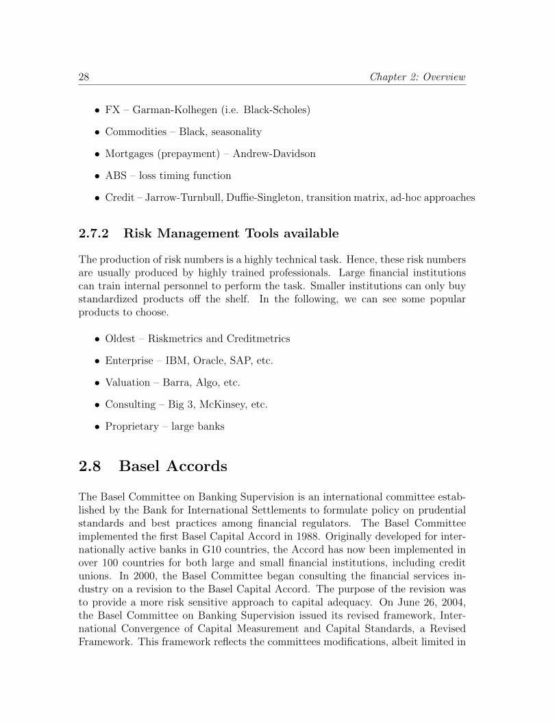
• FX – Garman-Kolhegen (i.e. Black-Scholes)
• Commodities – Black, seasonality
• Mortgages (prepayment) – Andrew-Davidson
• ABS – loss timing function
• Credit – Jarrow-Turnbull, Duffie-Singleton, transition matrix, ad-hoc approaches
2.7.2 Risk Management Tools available
The production of risk numbers is a highly technical task. Hence, these risk numbersare usually produced by highly trained professionals. Large financial institutionscan train internal personnel to perform the task. Smaller institutions can only buystandardized products off the shelf. In the following, we can see some popularproducts to choose.
• Oldest – Riskmetrics and Creditmetrics
• Enterprise – IBM, Oracle, SAP, etc.
• Valuation – Barra, Algo, etc.
• Consulting – Big 3, McKinsey, etc.
• Proprietary – large banks
2.8 Basel Accords
The Basel Committee on Banking Supervision is an international committee estab-lished by the Bank for International Settlements to formulate policy on prudentialstandards and best practices among financial regulators. The Basel Committeeimplemented the first Basel Capital Accord in 1988. Originally developed for inter-nationally active banks in G10 countries, the Accord has now been implemented inover 100 countries for both large and small financial institutions, including creditunions. In 2000, the Basel Committee began consulting the financial services in-dustry on a revision to the Basel Capital Accord. The purpose of the revision wasto provide a more risk sensitive approach to capital adequacy. On June 26, 2004,the Basel Committee on Banking Supervision issued its revised framework, Inter-national Convergence of Capital Measurement and Capital Standards, a RevisedFramework. This framework reflects the committees modifications, albeit limited in

Basel Accords 29
number, made in the Consultative Paper (CP3) issued in April 2003. In September2011, the Basel Committee revised its capital standards in what is referred to asBasel III.
2.8.1 Basel I
The bank must maintain capital (Tier 1 and Tier 2) equal to at least 8% of itsrisk-weighted assets.
• 0% - cash, central bank and government debt and any OECD government debt
• 0%, 10%, 20% or 50% - public sector debt
• 20% - development bank debt, OECD bank debt, OECD securities firm debt,non-OECD bank debt (under one year maturity) and non-OECD public sectordebt, cash in collection
• 50% - residential mortgages
• 100% - private sector debt, non-OECD bank debt (maturity over a year), realestate, plant and equipment, capital instruments issued at other banks OECD:Organisation for Economic Co-operation and Development
Tier 1 capital
Tier 1 capital is the core measure of a bank’s financial strength from a regulator’spoint of view. It is composed of core capital, which consists primarily of
• common stock and
• disclosed reserves (or retained earnings), but may also include
• non-redeemable non-cumulative preferred stock.
The Basel Committee also observed that banks have used innovative instru-ments over the years to generate Tier 1 capital; these are subject to stringent con-ditions and are limited to a maximum of 15% of total Tier 1 capital.
30 Chapter 2: Overview
Tier 2 capital (supplementary capital)
Tier 2 capital includes a number of important and legitimate constituents of a bank’scapital base. These forms of banking capital were largely standardized in the BaselI accord, issued by the Basel Committee on Banking Supervision and left untouchedby the Basel II accord. National regulators of most countries around the world haveimplemented these standards in local legislation. In the calculation of regulatorycapital, Tier 2 is limited to 100% of Tier 1 capital.
• Undisclosed reserves
• Revaluation reserves
• General provisions/general loan-loss reserves
• Hybrid debt capital instruments
• Subordinated term debt
Tier 3 capital
Tertiary capital held by banks to meet part of their market risks, that includes agreater variety of debt than tier 1 and tier 2 capitals. Tier 3 capital debts mayinclude a greater number of subordinated issues, undisclosed reserves and generalloss reserves compared to tier 2 capital. Tier 3 capital is used to support marketrisk, commodities risk and foreign currency risk.
• Banks will be entitled to use Tier 3 capital solely to support market risks.
• Tier 3 capital will be limited to 250% of a banks Tier 1 capital and have aminimum maturity of two years.
• This means that a minimum of about 28% of market risks needs to be sup-ported by Tier 1 capital that is not required to support risks in the remainderof the book;
http://www.bis.org/publ/bcbs128b.pdf
Capital Ratios
Capital ratios are various percentage measures that measure the financial health ofbanks. The use of ratios makes regulation a lot easier and ratios can be applied todifferent sizes of banks. The important capital ratios are given below.

Basel Accords 31
• Tier 1 capital ratio = Tier 1 capital / Risk-adjusted assets ≥ 6%
• Capital adequacy ratios (or total capital ratio) are a measure of the amountof a bank’s core capital expressed as a percentage of its risk-weighted asset.Capital adequacy ratio is defined as: Total capital (Tier 1 and Tier 2) / Risk-adjusted assets ≥ 10%
• Leverage ratio = Tier 1 capital / Average total consolidated assets ≥ 5%
• Common stockholders equity ratio = Common stockholders equity / Balancesheet assets
The following is the balance sheet of Lehman Brothers Inc. as of 2002 .
Lehman Brothers Inc.
as of 2002
Assets Liabilities
Cash 2,265 Short-term Debt 123
Securities 70,881 Other Securities 50,352
Coll Ag’mt 101,149 Coll ST Financing 121,844
Receivables 21,191 Payables 12,758
Real Estate 138 Long-Term Debt 7,990
Equity 3,152
Total 196,219 Total 196,219
million $
Figure 2.5: Balance Sheet of Lehman Brothers
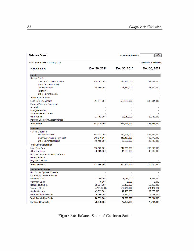
The following presents the balance sheet of Goldman from 2009 2011 (takenfrom Yahoo Finance). The equity ratio is 7.58%.
2.8.2 Basel II
Basel II is the second of the Basel Accords, (now extended and effectively supersededby Basel III), which are recommendations on banking laws and regulations issuedby the Basel Committee on Banking Supervision. Politically, it was difficult toimplement Basel II in the regulatory environment prior to 2008, and progress wasgenerally slow until that year’s major banking crisis caused mostly by credit defaultswaps, mortgage-backed security markets and similar derivatives. As Basel III was
32 Chapter 2: Overview
Figure 2.6: Balance Sheet of Goldman Sachs

Basel Accords 33
negotiated, this was top of mind, and accordingly much more stringent standardswere contemplated, and quickly adopted in some key countries including the USA.The main message of Basel II is the following three pillars:
Pillar 1: Capital Adequacy
Min. of 8% (but now credit, market & operational)
Pillar 2: Supervisory Review
Supervisors responsible for ensuring banks have sound internal processes toassess capital adequacy
Pillar 3: Market Discipline
Enhanced disclosure by banks
Sets out disclosure requirements
2.8.3 Basel III
Basel III is a comprehensive set of reform measures, developed by the Basel Com-mittee on Banking Supervision, to strengthen the regulation, supervision and riskmanagement of the banking sector. These measures aim to:
• improve the banking sector’s ability to absorb shocks arising from financialand economic stress, whatever the source
• improve risk management and governance
• strengthen banks’ transparency and disclosures.
The main message of Basel III is:
• Increased overall capital requirement: Between 2013 and 2019, the commonequity component of capital (core Tier 1) will increase from 2% of a banksrisk-weighted assets before certain regulatory deductions to 4.5% after suchdeductions. A new 2.5% capital conservation buffer will be introduced, as wellas a zero to 2.5% countercyclical capital buffer. The overall capital requirement(Tier 1 and Tier 2) will increase from 8% to 10.5% over the same period.
• Narrower definition of regulatory capital: Common equity will continue toqualify as core Tier 1 capital, but other hybrid capital instruments (upperTier 1 and Tier 2) will be replaced by instruments that are more loss-absorbingand do not have incentives to redeem. Distinctions between upper and lowerTier 2 instruments, and all of Tier 3 instruments, will be abolished. All

34 Chapter 2: Overview
non-qualifying instruments issued on or after 12 September 2010, and non-qualifying core Tier 1 instruments issued prior to that date, will both be dere-cognised in full from 1 January 2013; other non-qualifying instruments issuedprior to 12 September 2010 will generally be phased out 10% per year from2013 to 2023.
• Increased capital charges: Commencing 31 December 2010, re-securitisationexposures and certain liquidity commitments held in the banking book willrequire more capital. In the trading book, commencing 31 December 2010,banks will be subject to new stressed value-at-risk models, increased counter-party risk charges, more restricted netting of offsetting positions, increasedcharges for exposures to other financial institutions and increased charges forsecuritisation exposures.
• New leverage ratio: A minimum 3% Tier 1 leverage ratio, measured against abanks gross (and not risk-weighted) balance sheet, will be trialled until 2018and adopted in 2019.
• Two new liquidity ratios: A liquidity coverage ratio requiring high-qualityliquid assets to equal or exceed highly-stressed one-month cash outflows willbe adopted from 2015. A net stable funding ratio requiring available stablefunding to equal or exceed required stable funding over a one-year period willbe adopted from 2018.
2.9 Types of Capital
2.9.1 Regulatory capital
The Basel Committee on Banking Supervision (BCBS), on which the United Statesserves as a participating member, developed international regulatory capital stan-dards through a number of capital accords and related publications, which have col-lectively been in effect since 1988. In July 2013, the Federal Reserve Board finalizeda rule to implement Basel III in the United States, a package of regulatory reformsdeveloped by the BCBS. The comprehensive reform package is designed to help en-sure that banks maintain strong capital positions that will enable them to continuelending to creditworthy households and businesses even after unforeseen losses andduring severe economic downturns. This final rule increases both the quantity andquality of capital held by U.S. banking organizations. The Board also published theCommunity Banking Organization Reference Guide, which is intended to help small,non-complex banking organizations navigate the final rule and identify the changesmost relevant to them. The capital ratio is the percentage of a bank’s capital to its

Types of Capital 35
risk-weighted assets. Weights are defined by risk-sensitivity ratios whose calculationis dictated under the relevant Accord. Basel II requires that the total capital ratiomust be no lower than 8%. Under the Basel II guidelines, banks are allowed touse their own estimated risk parameters for the purpose of calculating regulatorycapital. This is known as the Internal Ratings-Based (IRB) Approach to capitalrequirements for credit risk. Only banks meeting certain minimum conditions, dis-closure requirements and approval from their national supervisor are allowed to usethis approach in estimating capital for various exposures.
2.9.2 Economic capital
As opposed to regulatory capital that is required by the governments or any regula-tory body, economic capital the firm needs to ensure that its realistic balance sheetstays solvent over a certain time period with a pre-specified probability. Therefore,economic capital is often calculated as value at risk. The balance sheet, in this case,would be prepared showing market value (rather than book value) of assets andliabilities. Economic capital is the amount of risk capital which a firm requires tocover the risks that it is running or collecting as a going concern, such as marketrisk, credit risk, and operational risk. Firms and financial services regulators shouldthen aim to hold risk capital of an amount equal at least to economic capital. It isthe amount of money which is needed to secure survival in a worst case scenario.Firms and financial services regulators should then aim to hold risk capital of anamount equal at least to economic capital.
2.9.3 Risk-adjusted return on capital (RAROC)
An adjustment to the return on an investment that accounts for the element ofrisk. Risk-adjusted return on capital (RAROC) gives decision makers the ability tocompare the returns on several different projects with varying risk levels. RAROCwas popularized by Bankers Trust in the 1980s as an adjustment to simple returnon capital (ROC). While there are many definitions of how RAROC should becalculated, one example provided by investopedia is: RAROC = (Revenue ExpensesExpected Loss + Income from Capital) / Capital where Income from Capital =(Capital Charges) (risk-free rate) and Expected loss = average anticipated lossover the measurement period.

36 Chapter 2: Overview
2.10 Appendix
2.10.1 Report on Excite@Homes bankruptcy
http://everything2.com/title/excite Excite (by then, Excite@Home) filed for bankruptcyon September 28, 2001. But let’s not start there, let’s start with 1999, when Excitewas second only to Yahoo as a pure web portal. Management calculated that theycould distinguish themselves by owning their own broadband pipes, and therebysurpass Yahoo and maybe even AOL in a few years. In a $6.7 billion deal, Excitemerged with @home, the leading provider of cable internet services. They estab-lished contracts with large cable companies making Excite the ’broadband portal’for most Americans with cable modems in 2000 and 2001. However, things wereturning ugly, as cash coming in from advertising contracts did not equal cash flow-ing out to employees and vendors. The company spent much of 2001 attempting toraise cash, selling divisions, selling convertible bonds (they raised $100 million fromPromethean Capital this way), and closing unprofitable units. Unfortunately, theycould not cut costs quickly enough to match the dropoff in advertising dollars. Evenafter firing half the staff, they were stuck with leases on the buildings those peoplehad worked from. From 2000q2 to 2001q2, ad revenue dropped more than 60%. Lotsof people were signing up for broadband, but the @home side of the business was toosmall to cover for the hemorrhaging Excite portal. The company needed to get cashfrom the outside, and they paid for it. Promethean Capital demanded immediaterepayment on the convertible bonds only a few months after buying them, claim-ing that Excite@Home had substantially misrepresented the state of their business.During the firesale, they sold Blue Mountain Arts, their online gift card unit, for$35 million to Gibson Greetings. Keep in mind that they had paid $780 million forBMA in late 1999. The fortunes of the company were closely tied to AT&T, andthey acted as AT&T’s broadband internet provider. This allowed them to negotiatean $85 million investment from AT&T in June 2001, but that was peanuts com-pared to the company’s burn rate, even after thousands of people had been fired. InAugust 2001, they fired their auditors, got a $50 million demand from Promethean,and had both Cox Cable and Comcast drop their service. Bankruptcy came thenext month. If you visit Excite.com today, you will see a website that looks like theold Excite portal, but it is an unrelated service that purchased the URL and logofrom Excite@Home after the bankruptcy filing. Business 2.0, August 28, 2001, USAToday, October 1, 2001, Various company press releases

Chapter 3
Hedging
3.1 What Is Hedging?
Hedging is the ultimate form of risk management. Hedging can be regarded as riskelimination. In other words, a perfect hedging should completely eliminate risk andresults in a risk-free portfolio. While hedging sounds pleasant, it is neither practical,nor necessary. In reality, even if perfect hedging did exist, nobody would want it,as no risk usually implies no return. If portfolio theory has taught us anything, itwould mean that we should maximize return at minimal risk.
Since hedging is risk elimination, it has become a perfect tool to develop pricingmodels. In an efficient market, the theory of hedging has been translated into pricingmodels. In other words, the cost of perfect hedging must be the price of the targetsecurity; otherwise arbitrage can take place and the efficient market is violated.Hence, by contradiction (which cannot exist), the cost of hedging must equal price ofthe target security. The most famous example is the Black-Scholes model developedin 1973.
Derivatives, namely options, futures (forwards), and swaps, are effective in-struments to eliminate risk. More interestingly, if used effectively, they can be usedto remove only the unwanted risk. This is known as the “static hedging”. Sincederivatives have maturity dates, once they expire, they need to be rolled over. Hencethey cannot be used for long term hedging purposes. For long term hedging needs,one can pursue “dynamic hedging” strategies. A dynamic hedging strategy requiresconstant trading and re-balancing the portfolio. The hedging is perfect only fora very short period of time (a day, an hour, or a few minutes) and then it mustbe redone in order to remain perfectly hedged. As a result, dynamic hedging canbe implemented only for securities that are very liquid. Over-the-counter (OTC)
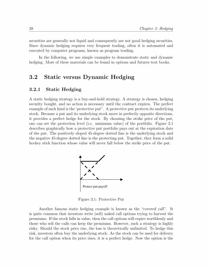
38 Chapter 3: Hedging
securities are generally not liquid and consequently are not good hedging securities.Since dynamic hedging requires very frequent trading, often it is automated andexecuted by computer programs, known as program trading.
In the following, we use simple examples to demonstrate static and dynamichedging. Most of these materials can be found in options and futures text books.
3.2 Static versus Dynamic Hedging
3.2.1 Static Hedging
A static hedging strategy is a buy-and-hold strategy. A strategy is chosen, hedgingsecurity bought, and no action is necessary until the contract expires. The perfectexample of such kind is the ‘protective put”. A protective put protects its underlyingstock. Because a put and its underlying stock move in perfectly opposite directions,it provides a perfect hedge for the stock. By choosing the strike price of the put,one can set the protection level (i.e. minimum value) of the portfolio. Figure 3.1describes graphically how a protective put portfolio pays out at the expiration dateof the put. The positively sloped 45-degree dotted line is the underlying stock andthe negative 45-degree dotted line is the protecting put. Together, they form a solidhockey stick function whose value will never fall below the strike price of the put.
Protect put payoff
Figure 3.1: Protective Put
Another famous static hedging example is known as the “covered call”. Itis quite common that investors write (sell) naked call options trying to harvest thepremiums. If the stock falls in value, then the call options will expire worthlessly andthose who sell the calls can keep the premiums. However, such a strategy is highlyrisky. Should the stock price rise, the loss is theoretically unlimited. To hedge thisrisk, investors often buy the underlying stock. As the stock can be used for deliveryfor the call option when its price rises, it is a perfect hedge. Now the option is the

Static versus Dynamic Hedging 39
target security and the stock is the hedging security. Figure 3.2 describes the payoffat the expiration date of the call option.
Covered call payoff
Figure 3.2: Covered Call
Buying the stock is expensive. An alternative is to buy another call optionwith a lower strike price. Since call prices are lower than stock prices, doing so cansave cost of hedging. It goes without saying that this cheaper hedging is not as idealas the hedging with stock. Figure 3.3 describes the result. As we can easily see thatthe payoff of this strategy (bull spread) is lower than the payoff of the covered call.
Bull spread w/ calls
Figure 3.3: Bull Spread
3.2.2 Dynamic Hedging
A dynamic strategy, as mentioned, requires constant trading and re-balancing theportfolio. A perfect example would be the covered call given earlier. In a staticstrategy, buying the stock can provide an effective hedge but it is very costly. Thereason why it is costly is that it keeps a very high payoff in the future (at theexpiration of the option). If we do not need such a high payoff, then the coveredcall strategy is not desirable. One can certainly go with an alternative which is a

40 Chapter 3: Hedging
bull spread to save cost (and give up high payoff). A really effective way is to dodynamic hedging using stock. This was first discovered by Fischer Black and MyronScholes in 1973.
Assume the stock price follows a stochastic process (see Chapter 1) as follows:
dS
S= µdt+ σdW
or
dS = µSdt+ σSdW
(3.1)
This is a very simple process for the stock. What it says is that the stock hasan expected return µ and volatility σ. dW is a Wiener process which is normallydistributed with mean 0 and variance dt. Since the option is a derivative contractwritten on the stock, it must be a function of the stock price. Hence, we can measurethe sensitivity of the option price change with respect to the stock price change:
∂C
∂S
For example, if ∂C/∂S is 0.25, which means any increase (or decrease) of thestock by $1 will result in a 25 cents increase (or decrease) in the option (or viceversa that every $1 change in option will result in $4 change in the stock), then wecan provide a very effective hedge by just doing a 1:4 hedge ratio. In other words,to protect a call option, we need to buy a quarter share of the stock. Of course theproblem is that the hedge ratio keeps changing as the stock price keeps changing.Consequently stock shares must be bought and sold constantly to match the hedgeratio. As a result, such hedging requires constant trading.1
As we can easily see, there is nothing that prevents us from using the samemethodology on other instruments. Indeed, such a method is proven to be universal.As long as there is an easy way to calculate ∂X/∂Y , one can effectively hedge Xwith Y or vice versa. In the above case, Black-Scholes has derived a closed-formformula for ∂C/∂S, which is “N(d1)” (details to be shown later) which is a standardnormal probability function.
1Note that the theory behind the strategy is actually quite profound. Black and Scholes firstshowed that such strategy is “self-financing”. That is, such a strategy does not incur any cost.Later, this is proven to follow the Martingale Representation Theorem.

Static versus Dynamic Hedging 41
Remarks
There are three remarks. First, such hedging is prefect, which it eliminates riskcompletely. If it eliminates all risk, then the portfolio is risk-free and should earnthe risk-free rate. If the portfolio requires no initial investment, then the portfolioshould not produce any return. This “no free lunch” or “arbitrage free” argumentis how pricing models are derived. In the case of the covered call, we can thenderive the pricing model for the call option. We can equally apply the same hedgingmethod for protective put and it will result in a put option model.
Second, if the risk is completely eliminated, then there is no purpose of doingany investment. One could easily just invest in the risk-free asset such as Treasurybills. As a result, the use of dynamic hedging is mostly for deriving pricing models,as opposed to finding the optimal hedging. Optimal hedging requires risk-returntradeoff which is not the purpose of dynamic hedging and hence is a different topic.
Third, when the market isn’t perfect, that is, the dynamic hedging cannotfully eliminate risk. In this situation, the dynamic hedging becomes a useful wayto eliminate the so-called “delta” risk. In other words, the dynamic hedging givesa “delta-neutral” portfolio. When the market isn’t perfect, frictions in the marketproduce what is known as the “gamma risk”. Without removing the delta risk,investors cannot see clearly how much the gamma risk is. By removing the deltarisk (via being delta-neutral), investors can now see clearly and then manage thegamma risk. Gamma risk cannot be hedged and often it produces attractive returns.Hence, Wall Street traders make money by taking gamma risk and managing it well.
3.2.3 Other Hedging Examples
Swaps/Forwards
Swaps are a very effective tool to hedge risk. The most commonly used hedgingstrategy is in the area of interest rate risk. A standard vanilla swap is a contractthat exchanges a set of fixed cash flows with a set of floating cash flows. Thesetwo legs of cash flows mimic fixed rate bond and floating rate bond. Given thatfloating rate bonds have almost no interest rate risk (i.e. duration), one can swapout interest rate risk by engaging in a fixed-floating interest rate swap.
Forwards are perfect hedges of the underlying assets. A forward contract canbe regarded as a long call and a short put. Previously we see how each can performa partial hedge. But together they become a forward contract which can guaranteea fixed cash flow (strike price) to the investor. In reality, there are very few liquid

42 Chapter 3: Hedging
forward markets but one can create one with calls and puts.2
Futures
Futures contracts can be effective in providing effective hedging. One application isknown as the “minimum variance hedging”. The idea is to use futures to hedge theunderlying. Often it is done with buying the underlying and shorting the futures.3
Let the hedge ratio be h and hence the portfolio value is:
V = S − hF
Then the change of the portfolio value is:
dV = dS − hdF
Given that such a hedge is not perfect, there is variance of the portfolio, whichcan be easily calculated as:
V[dV ] = σ2S + h2σ2
F − 2hρσSσF
The goal here is to minimize this portfolio variance with the best choice of thehedge ratio h. To achieve that, we simply take the derivative of the equation withrespect to the hedge ratio and set it to 0:
2hσ2F − 2ρσSσF = 0
which implies that:
h = ρσSσF
It turns out that this result is identical to the regression coefficient of dSrunning against dF .
2Foreign exchange and short term interest rate forward markets are liquid.3For commodity futures, it is difficult to short the underlying.

Part II
Market Risk


Chapter 4
Value At Risk
4.1 Introduction
Market risk is defined as the potential loss resulting from declining prices in thefinancial market. There are two dimensions to have a good overall grasp of themarket risk risk factors and drivers risk exposures.
Market risk consists of the following broad stochastic market risk factors (alsocan be regarded as asset classes):
• interest rates
• prepayment speeds (mortgage rates)
• credit spreads
• FX rates
• commodities
• equities
The two drivers of the market risk exposures are:
• investment position and
• volatility (including variances and co-variances)
It of great importance that we understand how to manage the size of invest-ment in each asset class (and hence the exposure to each risk factor) and the volatility

46 Chapter 4: Value At Risk
of each risk factor. It is of equal importance that we understand how the risk factorsmove over time and learn how to predict their movements. It is an on-going battlethat investors try to beat the markets while keep the risk under control.
Figure 4.10 is a simple organization chart that demonstrates how market riskis estimated.
Market Data Returns
Tests:
1. Visual
2. 2-std.dev.
Var-Covar
Matrix
Ω
Position Data DV01s (w) w’Ωw
Portfolio
VaR
Marginal
VaR
Component
VaR
Stress Tests
& Scenarios
Figure 4.1: Risk Management Flow Chart
As we can see from the diagram, the output of this system is a set of market riskmeasures, known as VaR (value at risk) lying at the bottom of the diagram. Thereare three types of VaR. The portfolio VaR (far right) is the final aggregated risknumber to be presented to the CEO of the company. Then, there is Absolute sub-portfolio VaR which is a number of VaR numbers of divisions of the company. As weshall demonstrate in details later, VaRs which are volatility based are not additive.Hence, the summation of all Absolute sub-portfolio VaRs is not the portfolio VaR.In order to force additivity, a series of Marginal sub-portfolio VaRs are created.These VaRs demonstrate how much each division of the company contributes to thetotal portfolio VaR.
Market Risk Management Toolbox:

Introduction 47
• Market Risk Factors Identification
• Sensitivity Analysis
• VaR for Market Risk: Riskmetrics (JP Morgan) 94
• Stress Testing and Scenario Analysis
• Economic Capital Adequacy Level
Relative VaR
• Report reveals important differences between VaR and Relative VaR
• Global Equities has the stand-alone VaR (11%), but relative to its benchmark,the smallest relative VaR (1%)
• Global FI Portfolio has smallest stand-alone VaR (5%) but highest relativeVaR (4%)
Marginal VaR measures how much risk a position adds to a portfolio or howmuch Portfolio VaR would change if a position is removed. Often the largest stand-alone risk positions are not the greatest contributors of risk hedges have a negativemarginal VaR. Identifies which position to eliminate entirely in order is most effectiveto reduce risk.
Component VaR is closely related to Marginal VaR. The sum of all componentVaRs add up to total Portfolio VaR. We should note that component VaR is liketo increase position weight by $1 and measure the change in overall portfolio VaRmultiply this change by position weighting.
4.1.1 An Example
Table 4.1 is a sample risk report. Note that Marginal VaRs add up to $946,078, notequal to the portfolio VaR. Although Asia ex Japan has the largest stand-alone VaR,it is the fourth largest contributor to risk, as measured by incremental VaR. Thebest 3 opportunities for reducing risk through hedges lie in US, Latam & Europe.
Diversification benefit = Overall Portfolio VaR – Sum of individual VaRs

48 Chapter 4: Value At Risk
Region Market Individual Marginal Component %
Value VaR VaR VaR Contribution
US 71.77 574,194 222,075 378,341 25.17%
S. Amer 10.26 512,944 220,114 369,626 24.59%
Europe 64.60 581,404 204,358 343,237 22.84%
Asia ex. Japan 12.69 589,734 196,046 317,346 21.11%
E. Europe 1.95 116,932 31,050 40,322 2.68%
Japan 19.57 195,694 48,012 30,068 2.00%
Africa 4.67 93,387 24,423 24,163 1.61%
Diversification (1,161,186)
Total 185.51 1,503,103 946,078 1,503,103 100.00%
Table 4.1: A Sample VaR Report
4.1.2 Limitations of VaR
Although VaR is the most widely used measure for market risk, it is far from perfectand presents many problems. First of all, VaRs are not additive. VaRs are trans-formations of standard deviations that are not additive. A fundamental assumptionthat future risk can be predicted from historical distribution is not realistic. Fur-thermore, it is vulnerable to regime shifts & sudden changes in market behavior.Finally, VaRs calculated by different methods have different limitations.
VaR gets me to 95% confidence. I pay my Risk Managers good salaries to lookafter the remaining 5% Dennis Weatherstone, former CEO, JP Morgan.
4.1.3 Stress Testing
Stress testing is designed to estimate potential economic losses in abnormal markets.It measures extreme market movements occur far more frequently than a normaldistribution suggest. It provides a more comprehensive picture of risk. Table 4.2presents a sample of what stress scenarios are.
4.1.4 Risk Reporting
An efficient risk reporting process is the final and the most important step of riskmanagement. An efficient risk reporting process is the foundation for clear and

Introduction 49
Standard Stress Test Scenario
Implied Volatility 20%
Equity Index 10%
Yield Curve Twist 25 bps
Parallel Yield Curve Shift 100bps
Table 4.2: Stress Test Scenarios
timely communication of risk across enterprise (Corporate, Business Unit, TradingDesk). What makes a good risk report?
• Timely
• Reasonably accurate
• Highlight portfolio risk concentrations
• Include a written commentary
• Be concise
4.1.5 External Disclosure
From Chase Manhattans Annual Report: Chase conducts daily VaR backtestingfor both regulatory compliance with the Basle Committee on Banking Supervisionmarket risk capital rules and for internal evaluation of VaR against trading revenue.
During the year, a daily trading loss exceeded that years trading VaR on 2days. This compares to an expected number of approximately 3 days. Consideringthe unsettled markets during the year, Chase believes its VaR model performed ata very high level of accuracy during the year.
4.1.6 The Basel Accord II
• Pillar 1: Capital Adequacy
– Min. of 8% (but now credit, market & operational)
• Pillar 2: Supervisory Review

50 Chapter 4: Value At Risk
– Supervisors responsible for ensuring banks have sound internal processesto assess capital adequacy
• Pillar 3: Market Discipline
– Enhanced disclosure by banks
– Sets out disclosure requirements
4.1.7 Capital Regulation
Figure 4.2 depicts the highlight of the capital adequacy ratio.
Capital
Required Exposure Risk Weight 8%
Market Risk Credit Risk
= ×××× ××××
Liquidity
Risk
(New) (Revised) (Unchanged)
Figure 4.2: Capital Adequacy
Risk Weighted Assets are computed by:
• RWA = Banking Book RWA + Trading Book RWA
• Banking Book RWA = Position × Risk Weighting
• Trading Book RWA = Market Risk Capital / 8%
4.2 Major Types of VaR
The concept of Value at Risk (or VaR) began with a thought that had been developedin JP Morgan in early 1990s about how their money managers can sleep well at night
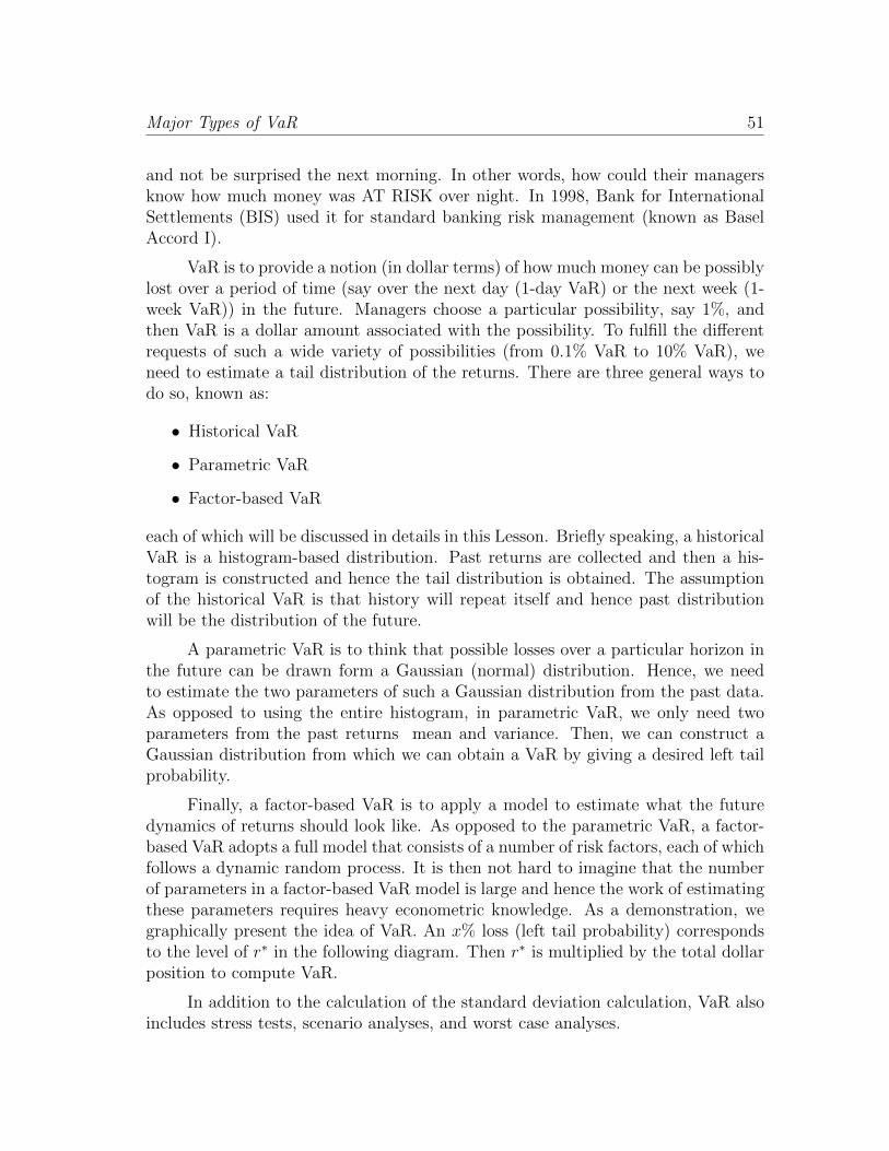
Major Types of VaR 51
and not be surprised the next morning. In other words, how could their managersknow how much money was AT RISK over night. In 1998, Bank for InternationalSettlements (BIS) used it for standard banking risk management (known as BaselAccord I).
VaR is to provide a notion (in dollar terms) of how much money can be possiblylost over a period of time (say over the next day (1-day VaR) or the next week (1-week VaR)) in the future. Managers choose a particular possibility, say 1%, andthen VaR is a dollar amount associated with the possibility. To fulfill the differentrequests of such a wide variety of possibilities (from 0.1% VaR to 10% VaR), weneed to estimate a tail distribution of the returns. There are three general ways todo so, known as:
• Historical VaR
• Parametric VaR
• Factor-based VaR
each of which will be discussed in details in this Lesson. Briefly speaking, a historicalVaR is a histogram-based distribution. Past returns are collected and then a his-togram is constructed and hence the tail distribution is obtained. The assumptionof the historical VaR is that history will repeat itself and hence past distributionwill be the distribution of the future.
A parametric VaR is to think that possible losses over a particular horizon inthe future can be drawn form a Gaussian (normal) distribution. Hence, we needto estimate the two parameters of such a Gaussian distribution from the past data.As opposed to using the entire histogram, in parametric VaR, we only need twoparameters from the past returns mean and variance. Then, we can construct aGaussian distribution from which we can obtain a VaR by giving a desired left tailprobability.
Finally, a factor-based VaR is to apply a model to estimate what the futuredynamics of returns should look like. As opposed to the parametric VaR, a factor-based VaR adopts a full model that consists of a number of risk factors, each of whichfollows a dynamic random process. It is then not hard to imagine that the numberof parameters in a factor-based VaR model is large and hence the work of estimatingthese parameters requires heavy econometric knowledge. As a demonstration, wegraphically present the idea of VaR. An x% loss (left tail probability) correspondsto the level of r∗ in the following diagram. Then r∗ is multiplied by the total dollarposition to compute VaR.
In addition to the calculation of the standard deviation calculation, VaR alsoincludes stress tests, scenario analyses, and worst case analyses.

52 Chapter 4: Value At Risk
Normal Distribution
Profits and Losses
x%
Figure 4.3: Value at Risk
4.2.1 Historical VaR
A historical VaR is one that is based upon only past return history and nothing else.A return history is called a histogram.
Histogram
A histogram is not necessarily Gaussian shape (usually not, known as the fat tails).To compute historical VaR is very simple. One simply sorts the possible losses in thepast (say 1 year which is roughly 250 observations) and choose from the worst tillthe pre-set percentage (say 4% VaR) is met (say the 10th observation). An exampleis given in Figure 4.4.
Historical VaR is very simple. When the asset mix of a firm is simple (e.g. onlystocks), historical VaR provides a somewhat reliable VaR number (if the process isstantionary that is past reflects future). When the asset mix is not so simple (e.g.stocks and bonds), then a histogram is easy to estimate (but may not be reliable toreflect the future).
However, historical VaR also suffers from a serious criticism. That is, historicalVaR is not forward looking. Past distributions may not be accurate representationsof the future. Other criticisms of historical VaR include:
• difficult to integrate VaRs of different securities (e.g. bond and stock)

Major Types of VaR 53
Figure 4.4: A Histogram Sample
• derivative assets have certain arbitrage-free relationship with its underlyingasset
• empirically very unstable
Examples
An ideal example for the historical VaR is the VaR of a single stock. An exampleof FaceBook (FB) 2008/5/17 ∼ 2009/1/2 has 157 stock prices which turn into 156returns. A histogram is summarized in Figure 4.5.
with the basic distribution statistics as in Table 4.3.
Historical VaR: there are 156 observations and 5% of that is 7.8 or 8. In otherwords, 5% historical VaR is the 8th worst observation which is 6.56%. This is oneday VaR. If we invest in 36,010 shares (or $1 million at 27.77 per share). Then thehistorical VaR is $65,620.
Some arguments are made against the above VaR number. Industry arguesthat return VaRs are not convenient to use and furthermore cannot be combined

54 Chapter 4: Value At Risk
0
0.05
0.1
0.15
0.2
0.25
0.3
0.35
-0.1244 -0.0944 -0.0645 -0.0345 -0.0046 0.0253 0.0553 0.0852 0.1152 0.1451 0.175
Series1
Series2
Figure 4.5: Facebook Example
Mean -0.002049130
Std.dev 0.040425118
Skew 0.204800858
Extra kurt 2.686877978
Table 4.3: Facebook Distribution Statistics
(known as the additive property). Hence, it is more conventional for the industry touse price changes as opposed to returns. The resulting VaR is known as the dollarVaR.
For the same example, the FB price change (∆S) histogram is plotted asfollows (as opposed to returns that is ∆S/S).
with the basic distribution statistics as in Table 4.4.
The 8th worst is $1.88. Say the number of shares is 36,010 (or $1 million at27.77 per share). Then the historical VaR is $67,699.
Historical VaR can work for any portfolio as long as there is data. In thefollowing I combine FB with WMT (Walmart) for the same period. Given thatboth FB and WMT are traded, the portfolio value (which is one share of FB andone share of WMT) can be computed and observed daily. Hence, for the same 157

Major Types of VaR 55
0
0.05
0.1
0.15
0.2
0.25
0.3
0.35
0.4
-4.2 -3.407 -2.614 -1.821 -1.028 -0.235 0.558 1.351 2.144 2.937 3.73
Series1
Series2
Figure 4.6: Facebook Example
Mean -0.06705130
Std.dev 1.02337596
Skew -0.50810290
Extra kurt 3.04349237
Table 4.4: Facebook Distribution Statistics
days, the return histogram for the portfolio is given in Figure 4.7.
with the basic distribution statistics in Table 4.5.
The eighth worst observation is 2.29%. This is the portfolio one-day VaR.Assuming $1 million investment, the historical VaR is $22,857.
Similarly, we can do the dollar VaR for the portfolio and the histogram is inFigure 4.8.
with the basic distribution statistics in Table 4.6.
The eighth worst observation is −2.14. This is the portfolio one-day VaR.Assuming $1 million investment, the historical VaR is $21,877.
The benefit of the historical VaR is that we do not need to compute the large

56 Chapter 4: Value At Risk
0
0.05
0.1
0.15
0.2
0.25
0.3
-0.039 -0.031 -0.023 -0.015 -0.007 0.0004 0.0083 0.0161 0.0239 0.0318 0.0396
Series1
Series2
Figure 4.7: Facebook and Walmart
Mean 9.5066E-05
Std.dev 0.01273587
Skew -0.08926460
Extra kurt 0.27394334
Table 4.5: Combined Distribution Statistics
variance-covariance matrix as the parametric VaR does (to be discussed in the nextsection). Historical VaR, we have seen, looks at only the 8th (i.e. the 5th percentile)observation of the history of the portfolio. However, to use the historical VaR, theremust be data for all the constituents in the portfolio.
Also to be noted is that historical VaR does not suffer from the criticism ofthe fat tails. Given that it takes a chosen percentile from the left tail, both skewnessand kurtosis are automatically incorporated and fat tails are supported.
The same principle can be applied to a stock (or any “primary” asset, or knownas a “basic asset class”) and its derivatives (or any derivative assets), such as anoption like call or put. But often the derivatives are traded in an illiquid market(over the counter) and its prices are not always available. In this case, we can use a

Major Types of VaR 57
0
0.05
0.1
0.15
0.2
0.25
0.3
-3.62 -2.879 -2.138 -1.397 -0.656 0.085 0.826 1.567 2.308 3.049 3.79
Series1
Series2
Figure 4.8: Facebook and Walmart (Dollar Change)
Mean 0.00923077
Std.dev 1.21440841
Skew -0.08985380
Extra kurt 0.23078100
Table 4.6: Combined Distribution Statistics (Dollar Change)
model to “fill in” any missing prices there are in the history. The reason that we cando so is because there is a strong functional relationship between derivatives andtheir underlying assets. In the past several decades, numerous pricing models havebeen developed to accurately estimate the derivative prices from their underlyingasset values. Later, we shall demonstrate several classical such pricing models. Here,we use the most famous Black-Scholes model for call option as a demonstration.
The Black-Scholes model for a call option on stock can be written as
Ct = StN(d1)− e−r(T−t)KN(d2) (4.1)
where St is the current stock price (assuming that t is the current time), K is thestrike price, r is the constant risk-free rate (which can be relaxed to be random

58 Chapter 4: Value At Risk
in order to match reality), σ is the volatility (which is standard deviation of stockreturns), T−t is the time till maturity of the option (assuming that T is the maturitytime), N(·) is the standard normal probability, and
d1 =lnSt − lnK + (r + σ2/2)(T − t)
σ√T − t
d2 = d1 − σ√T − t =
lnSt − lnK + (r − σ2/2)(T − t)σ√T − t
The standard normal probability N(·) can be found in Excel as NORMS-DIST(x) where x is either d1 or d2.
With model-generated option prices, we can do the historical VaR as follows.The following example is a histogram where the stock prices are collected historicallyand yet the call option prices are computed by the Black-Scholes model. The bluebars represent the distribution of the FB stock. The red bars represent the calloption. The hollow bars represent the portfolio that consists of one stock and oneoption. The bin for each histogram is given as follows (10 equal intervals). Notethat the histogram of the stock is the same as the one shown earlier.
bin FB FB call Portfolio
1 -4.2 -4.1522 -8.3438
2 -3.407 -3.4974 -6.8968
3 -2.614 -2.8426 -5.4499
4 -1.821 -2.1878 -4.0029
5 -1.028 -1.533 -2.556
6 -0.235 -0.8782 -1.109
7 0.558 -0.2234 0.33793
8 1.351 0.43136 1.78488
9 2.144 1.08615 3.23183
10 2.937 1.74094 4.67878
11 3.73 2.39573 6.12573
Table 4.7: Facebook and Call
We can see that the distribution of option price changes is highly skewed.Certainly this is no surprising as options are leveraged derivative contracts.
The 8th worst price change (5% of the histogram) of the portfolio is −3.46. Ifthe call option data are available, one could do a true historical VaR using actualoption data.

Major Types of VaR 59
0
0.05
0.1
0.15
0.2
0.25
0.3
0.35
0.4
0.45
1 2 3 4 5 6 7 8 9 10 11
FB Stock FB 20 6-mon Call Portfolio
Figure 4.9: Facebook and Call
4.2.2 Parametric VaR
Once not all securities have historical data, historical VaR cannot apply. As aresult, we can use parametric VaR. That is, we employ a model and no longer relyon history to compute VaR. The simplest parametric VaR model is the adoption ofthe Gaussian distribution.
Parametric VaR also has other advantages such as:
• all securities are modeled under a consistent framework (note that historicalVaR combines securities values brute-forced, which could combine apples withoranges)
• parametric VaRs are scalable (square root of time)
An early concept of parametric VaR was one standard deviation value. In otherwords, if the market swings by one standard deviation, how much money would belost. In a normal distribution, one standard deviation is the 16th percentile. Inother words, one standard deviation drop in value can happen with 16% probability.Similarly, a two-standard deviation loss is 2.3% probability. If the manager wantsto know what is 1% (or 5%) likely loss, under normal distribution, it is 2.326 (1.645)

60 Chapter 4: Value At Risk
standard deviations. If one standard deviation is $100,000, then with 1% probabilitythe portfolio will lose more than $233,000.
Example (continued)
Continue with the FB example, we know from the distribution statistics that themean return is −0.205% and the standard deviation is 0.0404. Hence the 95% VaRis:
−6.86% = −0.205%− 1.645× 0.0404
If position is $1 million, then VaR is $68,543 for parametric (compared with$65,620 for historical VaR). For the VaR of 1 week, we must do historical VaRseparately, but parametric VaR is simply 68, 543 ×
√7 = 181, 348. Under dollar
VaR, we have
−$1.75 = −0.067− 1.645× 1.0234
using the mean and standard deviation given in the previous section. For $1 millionposition (i.e. 36,010 shares), this is $63,030 (compared with $67,699 for historicalVaR). Certainly, this VaR can be scaled by the square root of the number of days.
Two-stock example
For two stocks (FB and WMT), the return parametric VaR is $20,854 (comparedwith the historical VaR of $22,857) and the dollar parametric VaR is $20,326 (com-pared with the historical VaR of $21,877).
A portfolio of two stocks, say 40%-60%. Historical VaR is fine as long as thehistory of two stocks exists. But if not (say one has a few missing values) then wecannot do historical VaR (of course we can back-fill these values but that is up tothe assumptions of back-filling.
We could do parametric VaR using the portfolio means and standard deviation,defined as follows:
µP = w1µ1 + w2µ2
σP =√w2
1σ21 + 2w1w2ρσ1σ2 + w2
2σ22
(4.2)

Major Types of VaR 61
where µ represents mean and σ represents standard deviation of stock returns. ρis the correlation coefficient between the two stocks. Note that ρσ1σ2 is the covari-ance between the two stocks (usually a notation σ12 is used). We can convenientlycompute the covariance from data using an Excel function COVAR(array1, array2)
without calculating the correlation coefficient.
Continue the same example in the previous section. The correlation betweentwo series of returns is -0.1399. Hence, we can compute the variance-co-variancematrix to be:
0.0000983 -0.0000560
-0.0000560 0.0016342
Table 4.8: Variance-Covariance Matrix for Returns
The portfolio consists of 10,223 shares of each stock (at $28.76 for FB and$69.06 for WMT) and hence $1 million in total. This represents 70% WMT and30% FB.
As a result, the portfolio mean and standard deviation (using equation (4.2))are: −0.0001561 and 0.0131 respectively and the 95% VaR is −0.021710, or $21,710(compared to $22,857 historical VaR).
For the price change VaR it is best to use number of shares as weights. To seethat:
∆V = n1∆S1 + n2∆S2
Compute the variance of the price change:
var[∆V ] = n21σ
21 + 2n1n2σ12 + n2
2σ22
= [n1 n2]
[σ2
1 σ12
σ12 σ22
][n1
n2
]
where σ presents dollar variances and covariances. The variance-covariance matrixfor the price change becomes Table 4.9.
As a result, the portfolio standard deviation is $11,824.63 and the 95% VaRis $19,452 (compared to $21,877), ignoring the mean.

62 Chapter 4: Value At Risk
0.4911838 -0.1016057
-0.1016057 1.0472983
Table 4.9: Variance-Covariance Matrix for Price Changes
n stock example
The portfolio is characterized by a set of portfolio weights: w1, · · · , wN . The ex-pected return of the portfolio is:
∑N
i=1wiµi = w′1×NMN×1 (4.3)
and the variance of the portfolio is:
(w′1×NΩN×NwN×1
)1×1
(4.4)
where Ω is the var-cov matrix of stocks. Hence the portfolio VaR is 1.645 (95%) or2.326 (99%) multiplied the square root of the following variance. Note that for theprice change VaR weights are shares.
An example of combining stock and option
It is quite common for a portfolio to contain derivative assets. This could be yieldenhancements (i.e. using derivatives to increase leverage) or hedging (i.e. usingderivatives to cancel exposures). As a result, we must know how a derivative assetrelates to its underlying asset.
In derivatives pricing, Black and Scholes, in their seminal work which wonthem the Nobel prize in 1997, show that delta hedging is a perfect way to reducethe risk of a derivative asset completely. In other words, one can build a portfoliowith a derivative asset and its underlying asset and reach 0 risk. However, in asituation of imperfect hedging or yield enhancement, there is still risk and VaR canstill be computed.
The parametric VaR can be computed easily. Assume a portfolio of 1 FB stockand 1 at-the-money call option (on the same stock). The information of the stockis: S = 27.77, K = 20, r = 0, σ = 0.4, T − t = 0.5. The option value is computedas:

Major Types of VaR 63
C = SN(d1)− e−r(T−t)KN(d2)
= 27.77× 0.9035− 1× 20× 0.8459
= 8.17
(4.5)
Now, you need to calculate (dollar) VaR of your portfolio. The change of valueof your portfolio can be computed as:
dV = dS + dC
= dS + ∆dS
= dS(1 + ∆)
(4.6)
where ∆ = N(d1) is the delta of your call. As a result, the volatility of dV is:
Std.Dev.(dV ) = Std.Dev.(dS)× (1 + ∆)
= S × σ × (1 + ∆)
= 27.77× 0.4× (1 + 0.9035)
= 21.14
(4.7)
As a result, the six-month portfolio VaR is 21.14× 1.645 = 34.78. One couldscale this parametric VaR to one-day to be 34.68/
√126 = 3.10 (half year is 126
business days.) Note that the historical VaR computed previously is $3.46 so thisparametric VaR is smaller. This is one share of stock and one share of option.If we have 100 shares of stock and 20 shares of option, then the VaR becomes27.77× 0.4× (100 + 20× 0.9035) = 1311.52.
Note that if we short the call option, then the option contract would serve as ahedge. In this way, we drastically reduce the risk. The standard deviation becomes:
Std.Dev.(dV ) = Std.Dev.(dS)× (1−∆)
= S × σ × (1−∆)
= 27.77× 0.4× (1− 0.9035)
= 1.07
(4.8)
and the 5% six-month portfolio VaR 1.07× 1.645 = 1.76. Scaling it to one-day (126days), we obtain 0.16. Now we know that using derivatives can completely removerisk by selecting proper shares of the option to buy (known as the hedge ratio).Assume that we buy 1,000 shares of the stock (which is worth $27,770 today) andwould like to find out how many shares of 20-strike call option to short. Then theprice change equation becomes:

64 Chapter 4: Value At Risk
Std.Dev.(dV ) = S × σ × (1, 000− nC∆)
= 0(4.9)
We would like the risk to be 0 and hence we can easily solve for the numberof shares nC to short which is equal to nC = 1000
∆= 1106.78, or roughly 1,107
shares. In other words, by shorting 1,107 shares of call option, the risk is completelyeliminated.
4.2.3 Factor Model Based VaR
Historical VaR is not very useful. When the asset mix of a firm is simple (e.g.only stocks), it is easier to estimate a historical probability distribution. But if theasset mix is not so simple (e.g. stocks and bonds), then a historical probabilitydistribution is not so easy to estimate. Especially if some assets are not liquidlytraded, then there is no history of these assets. Then the historical VaR methodwill fail.
Historical VaR also suffers from a serious criticism. That is, historical VaR isnot forward looking. Past distributions may not be accurate representations of thefuture. Hence, it is important that we forecast what future distribution should looklike. Other criticisms of historical VaR include:
• security returns are usually not normal
• assuming a correlation (again, this is normal-based) is inaccurate
• difficult to integrate VaRs of different securities (e.g. bond and stock)
• derivative assets have certain arbitrage-free relationship with its underlyingasset
• empirically very unstable
Given the above obvious reasons, VaR models have become parametric. Thatis, we employ a model and no longer rely on history to compute VaR. The stan-dard VaR model used by the financial industry is a linear factor model. Althoughthe details vary, a VaR model is typically a linear model in widely observed eco-nomic variables. As a result, the VaR models used today are connected with P&Lattributions.
From P&L attributions, we know that there are a number of explanatoryfactors, such as FX rates, interest rates, equity indicies, various volatilities, · · · , etc.

Major Types of VaR 65
To put all assets under one VaR umbrella, we need a flexible and yet manageablemodel. First of all the risks must be additive. Standard deviations are NOT additive.So we must use something else. We use delta, or more generally, the first ordersensitivity with respect to the underlying risk factor.
Principal Component Analysis
A PCA (Principal Component Analysis) is implemented to decide how many signif-icant factors that affect the equity market. Given N stocks, a PCA could extractonly a handful (say 3∼5) of factors (decided by the eigenvalues of the PCA). Theseare known as common factors. One can think of these common factors as macroeco-nomic variables such as inflation, GDP, exchange rates, etc. However, these factorsextracted using PCA do not have those interpretations (in fact, this the main draw-back of the PCA methodology, which is the factors are unintepretable.) Despite ofthis drawback, PCA is a “honest” methodology. In other words, PCA looks at thedata of equity returns and recognizes (from how highly or lowly these equity returnsare correlated) how many factors (K) are really needed to explain N stocks.1
To use PCA, one must assume a linear factor-based return generating modelof the following:
Ri,t = bi,1F1,t + bi,2F2,t + · · ·+ bi,NFN,t (4.10)
In matrix form (which is important when we use Excel to carry out calcula-tions), we can write this as:
R11 R12 · · · R1T
R21. . .
.... . .
RN1 RN2 · · · RNT
=
b11 · · · b1N...
...bN1 · · · bNN
F11 F12 · · · F1T
F21...
FN1 FN2 · · · FNT
RN×T = BN×N × FN×T
(4.11)
PCA takes the return matrix (i.e. R and returns a set of coefficients (eigen-vectors) which are the known as factor loadings or “factor betas”. In other words,a PCA outputs an N × N matrix B. Depending upon the matrix arrangement,sometimes it is convenient to arrange the return matrix as an T ×N matrix:
1That is, PCA can decide how many dimensions (K) are needed to expand the equity spacewhich is N dimensions.

66 Chapter 4: Value At Risk
R11 R21 · · · RN1
R12. . .
.... . .
R1T R2T · · · RNT
=
F11 F21 · · · FN1
F12...F1T F2T · · · FNT
b11 · · · bN1
......
b1N · · · bNN
R′T×N = F′T×N ×B′N×N
(4.12)
Hence, depending on what return matrix (either N×T or T×N) is fed to PCA,the corresponding factor loading matrix (either B or B′) will be generated. As aresult, we can obtain the factor time series by inverting the beta matrix as follows:
B−1N×N ×RN×T = FN×T
or
R′T×N × (B′)−1N×N = F′T×N
(4.13)
Note that factor loading matrix is an orthogonal matrix (i.e. inverse equalstranspose or B′ = B−1)). Hence, we can write R′ ×B = F′.
Let us have a simple 2×2 example where only two stocks are used. The returnsof the two stocks are given as follows:
2 Stock PCADate Stock 1 Stock 2
2/9/2006 4.32 4.522/10/2006 4.36 4.532/13/2006 4.38 4.552/14/2006 4.42 4.552/15/2006 4.39 4.55
· · · · · · · · ·
After running PCA, we obtain the factor loading matrix (B):
0.970203 -0.2422950.242295 0.970203
To solve for the factor values, we can solve for the following equations:
0.97× F11 − 0.24× F21 = 4.32
0.24× F11 + 0.97× F21 = 4.52

Major Types of VaR 67
and hence F11 = 5.29 and F21 = 3.34.
So when we pre-multiply the return matrix (R′) by the factor loading matrix,we should get the factor value matrix (R′ ×B = F′):
2 Stock PCADate Factor 1 Factor 2
2/9/2006 5.286448 3.3386022/10/2006 5.327679 3.3386122/13/2006 5.351929 3.3531712/14/2006 5.390737 3.3434792/15/2006 5.361631 3.350748
· · · · · · · · ·
This matrix operation is quite easy in Excel. MMULT(· · · , · · · ) can performthe above matrix multiplication easily. Note that the right area in Excel must beblocked and then use Ctrl-Shft-Entr.
If all N stocks are independent, then PCA will find identical eigenvalues andthere is no benefit of dimension reduction (i.e. K = N). However, if stocks arehighly correlated, then PCA will find fast-decaying eigenvalues, indicating that thefirst few factors can explain most of the returns (i.e. K < N). In this case, we findbenefits of using PCA.
Theoretically, this can be explained by the following equation:
Ri,t = bi,1F1,t + bi,2F2,t + · · ·+ bi,NFN,t
= µi + (bi,1f1,t + · · ·+ bi,KfK,t) + ei,t
or, dPi,t = ai +∑K
k=1bi,kfk,t + ei,t
(4.14)
with µi =∑K
k=1 bi,kE[Fk]. Note that fj = Fj − E[Fj] and hence E[f1] = 0, E[f2] = 0and E[ei] = 0.
As we can see, only K factors (out of potentially N factors) are chosen and therest are thrown into the “error term”. By making the assumptions that the errorterm (which consists of unimportant factors) is negligible, we only need part of thefactor loading matrix: BN×K and hence we have the variance-covariance matrix ofthe stocks being replaced with the variance-covariance of the factors as follows:
ΩP (N×N) = BN×KΩF (K×K)B′K×N (4.15)
where ΩP is the variance-covariance matrix of stocks. These factor values are alsoused for simulations. Note that only the significant factors will be used for predicting

68 Chapter 4: Value At Risk
stock returns. So out of N factors, only K actors are significant and used. The restare treated as errors (idiosyncratic).
Portfolio returns over time are computed as:
∑N
i=1wiRi,t (4.16)
so the entire time series of the portfolio returns can be computed as:
w′1×NRN×T (4.17)
Using PCA, the portfolio is:
w′1×NRN×T = w′1×NBN×KFK×T + w′1×NeN×T (4.18)
and hence the portfolio variance:
σ2P =
(w′1×NΩP (N×N)wN×1
)1×1
(4.19)
can be re-expressed in terms of factors as follows:
(w′1×NBN×KΩF (K×K)B
′K×NwN×1
)1×1
(4.20)
As a result, the VaR number (at α, say 5%) of the portfolio is the followingcalculation:
VaR = N−1(α)×√w′ΩPw
= N−1(α)×√w′BΩF B′w
(4.21)
This method reduces the computation complexity of an N × N variance-covariance matrix to a K ×K variance-covariance matrix. Furthermore, the factormodel can be estimated easily.
In simulations, factors are assumed normal with the means and variances esti-mated by the PCA. Error terms are also normal with mean 0 and variances estimatedby the PCA. This way, we can construct the simulated return series of the stocksand estimate the VaR that is forward-looking.

Major Types of VaR 69
Regression Model
PCA has a severe disadvantage that the factors carry no intuitive meaning. Oftenmodelers need to run analyses to investigate what these factors mean. The usualmethod is correlate factor values with known economic indicators (believing thatthese factors reflect fundamental economy).
An alternative is to directly use known economic indicators as factors. Thenwe simply run regressions with these observable economic indicators as independentvariables.
rj = aj + bj1rF1 + bj2rF2 + · · ·+ ej (4.22)
where variables in the regression can be any chosen economic variables. Or onecould use the popular Fama-French factors where the common factors are posted onthe French website. The Fama-French factors have gained tremendous popularityover the years and have become the standard of empirical asset pricing.
A More Complex Fixed Income Example
In this example, we limit ourselves to only interest rate risk. Let the instantaneousrate follow a three-factor model (where factors are independent of one another):
r = y1 + y2 + y3 (4.23)
where factors are independent and each factor yi is assumed to follow either theVasicek or the CIR model as follows:
dyk = αk(µk − yk)dt+ σkdWk Vasicekdyk = αk(µk − yk)dt+ σk
√ykdWk CIR
(4.24)
where k = 1, 2, 3. Under either model, we have a closed form solution to the discountfactor (for each k):
Yk(t, T ) = Et[exp
−∫ T
t
yk(u)du
]= Ak(t, T ) exp−Bk(t, T )yk(t)
(4.25)
Under the Vasicek model we have the following closed-form solutions to Akand BK :

70 Chapter 4: Value At Risk
− lnAk(t, T ) =
(µk −
σkλkαk− σ2
k
2α2k
)(T − t−Bk(t, T )) +
σ2kBk(t, T )2
4αk
Bk(t, T ) =1− e−αk(T−t)
αk
(4.26)
and under the CIR model we have:
Ak(t, T ) =
[2γke
(αk+λk+γk)(T−t)/2
(αk + λk + γk) (eγk(T−t) − 1) + 2γk
]2αkµk/σ2k
Bk(t, T ) =2(eγk(T−t) − 1
)(αk + λk + γk) (eγk(T−t) − 1) + 2γk
γk =√
(αk + λk)2 + 2σ2k
(4.27)
where λ is the market price of risk. The fundamental factors, yks, span the entirerisk free fixed income universe. Hence, the job now is to estimate these factors,namely we need to estimate αk, µk, σk, and λk for k = 1, · · · , K. To estimate this,we need to implement the MLE (maximum likelihood estimation). In an exerciseat the end of this Chapter, readers can practice these calculations with parametersgiven (estimated by Chen and Yeh and Chen and Scott).
Now because the factors are assumed independent, the risk-free discount factorcan be written as:
P (t, T ) = Et[exp
−∫ T
t
r(u)du
]= Y1(t, T )Y2(t, T )Y3(t, T )
= A1(t, T )A2(t, T )A3(t, T ) exp−B1(t, T )y1 −B2(t, T )y2 −B3(t, T )y3(4.28)
Then the price change can be easily derived as:
dP (t, T ) = (−B1(t, T )dy1 −B2(t, T )dy2 −B3(t, T )dy3)P (t, T ) (4.29)
Define an arbitrary coupon bond (symbolized as j where j = 1, · · · , J) as:
Πj = Π(cj, Tnj) = cj∑nj
i=1P (t, Ti) + P (t, Tnj) (4.30)

Major Types of VaR 71
where nj is the number of coupons paid by bond j and cj is same coupon at eachtime Ti.
Then, we can derive the price change of a coupon bond as:
dΠj = cj∑nj
i=1dP (t, Ti) + dP (t, Tn)
= cj∑nj
i=1(−B1(t, Ti)dy1 −B2(t, Ti)dy2 −B3(t, Ti)dy3)P (t, Ti)
+ (−B1(t, Tn)dy1 −B2(t, Tn)dy2 −B3(t, Tn)dy3)P (t, Tn)
= a1dy1 + a2dy2 + a3dy3
(4.31)
where for k = 1, 2, and 3,
ak = −cj∑nj
i=1Bk(t, Ti)P (t, Ti)−Bk(t, Tn)P (t, Tn)
Hence, we can easily compute variances and covariances as:
var[dP ] = P 2(B21v
21 +B2
2v22 +B2
3v23)
cov[dP, dΠ] = b1v21 + b2v
22 + b3v
23
var[dΠ] = a21v
21 + a2
2v22 + a3
3v23
(4.32)
where (for k = 1, 2, 3)
bk = ak(−Bk)P
v2k = var[dyk]
(4.33)
If we invest n1 units in P and n2 units in Π,2 then the 5% VaR is:
VaR5% = 1.645×
√√√√[n1, n2]
[var[dP ] cov[dP, dΠ]
cov[dP, dΠ] var[dΠ]
][n1
n2
](4.34)
To write it in a matrix form for the var-cov matrix:
2Note that the total investment amount is V = n1P + n2Π and weights are w1 = n1P/V andw2 = n2Π/V .
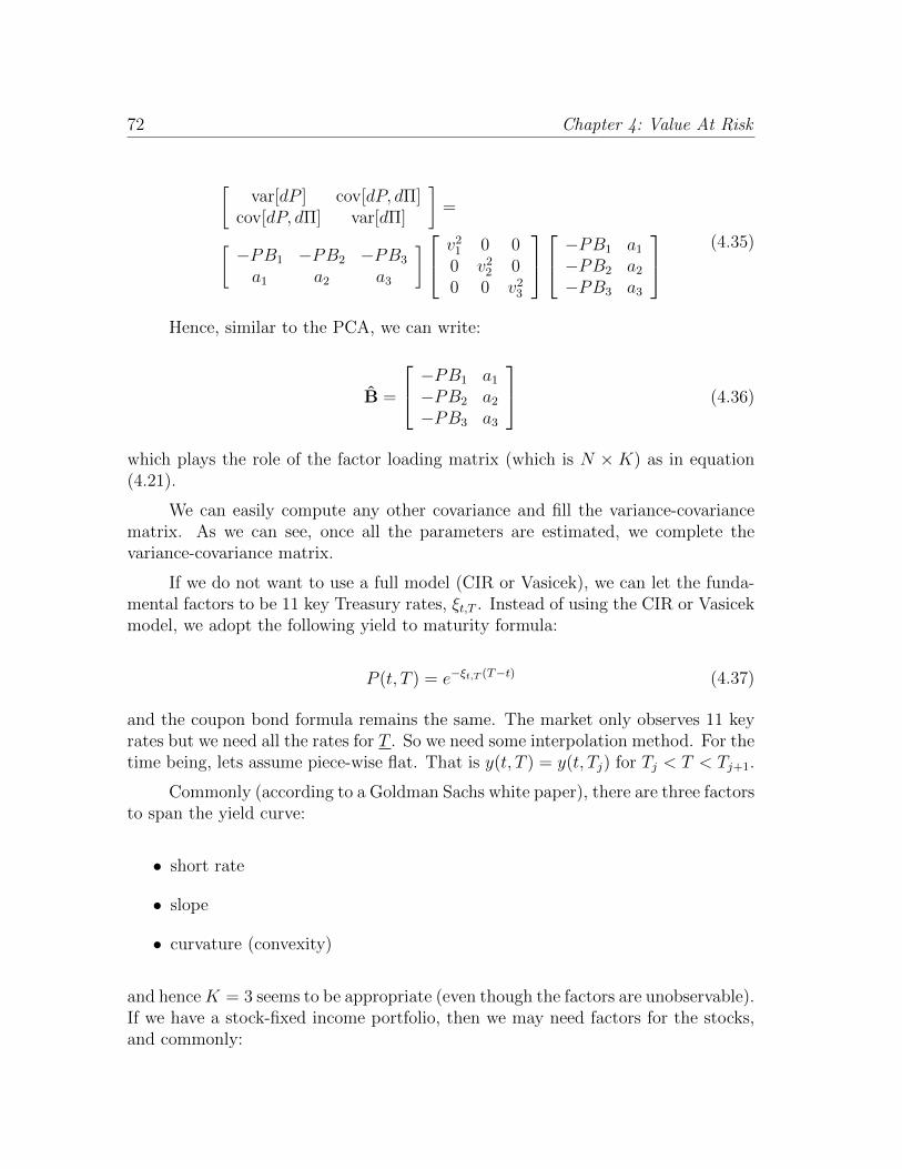
72 Chapter 4: Value At Risk
[var[dP ] cov[dP, dΠ]
cov[dP, dΠ] var[dΠ]
]=
[−PB1 −PB2 −PB3
a1 a2 a3
] v21 0 00 v2
2 00 0 v2
3
−PB1 a1
−PB2 a2
−PB3 a3
(4.35)
Hence, similar to the PCA, we can write:
B =
−PB1 a1
−PB2 a2
−PB3 a3
(4.36)
which plays the role of the factor loading matrix (which is N ×K) as in equation(4.21).
We can easily compute any other covariance and fill the variance-covariancematrix. As we can see, once all the parameters are estimated, we complete thevariance-covariance matrix.
If we do not want to use a full model (CIR or Vasicek), we can let the funda-mental factors to be 11 key Treasury rates, ξt,T . Instead of using the CIR or Vasicekmodel, we adopt the following yield to maturity formula:
P (t, T ) = e−ξt,T (T−t) (4.37)
and the coupon bond formula remains the same. The market only observes 11 keyrates but we need all the rates for T . So we need some interpolation method. For thetime being, lets assume piece-wise flat. That is y(t, T ) = y(t, Tj) for Tj < T < Tj+1.
Commonly (according to a Goldman Sachs white paper), there are three factorsto span the yield curve:
• short rate
• slope
• curvature (convexity)
and henceK = 3 seems to be appropriate (even though the factors are unobservable).If we have a stock-fixed income portfolio, then we may need factors for the stocks,and commonly:

Marginal and Component VaR 73
• market index (e.g., S&P 500)
• industry indices (e.g., SIC code 9 industries)
PCA can easily incorporate the factors in a augmented matrix. For parametricmodels, we may consider the Merton-Rabinovitch model (1973-1989) where bothstocks and interest rates can be random.
4.3 Marginal and Component VaR
Given that VaR is such a powerful and intuitive risk measure, it is then quite im-portant to break down this number into various divisions of the company in orderto see which division of the company is responsible for the most risk born by thecompany. This is understood as the component VaR.
A three-stock example in the following demonstrates how each component VaRis calculated.
σ2P =
[x1 x2 x3
] σ11 σ12 σ13
σ12 σ22 σ23
σ13 σ23 σ33
x1
x2
x3
=
x2
1σ11 + x1x2σ12 + x1x3σ13 → X1
x1x2σ12 + x22σ22 + x2x3σ23 → X2
x1x3σ13 + x2x3σ23 + x23σ33 → X3
(4.38)
Taking April 1, 2003 till October 6, 2009 weekly prices of JNJ (Johnson &Johnson), JPM (JP Morgan), and KO (Coke Cola), we obtain the following variance-co-variance matrix in Table 4.10.
JNJ JPM KO
JNJ 0.000514 0.000575 0.000372
JPM 0.000575 0.004493 0.000631
KO 0.000372 0.000631 0.000714
Table 4.10: JNJ, JPM, KO
We further assume that the investment amounts on these stocks are $10,000(35.71%), $6,000 (21.42%), and $12,000 (42.86%). The portfolio standard deviationin percent terms is 0.02685 and in dollar terms $751.852. As a result, the 5% VaRis $1,236.69.

74 Chapter 4: Value At Risk
To calculate the three component VaRs for JNJ, JPM, and KO, we first notethat x1 = 10, 000, x2 = 6, 000, and x3 = 12, 000. Hence, X1 = 130, 635, X2 =241, 674, and X3 = 192, 972, which sum to a total of 565,281.399. As a result,each X1 ∼ X3 accounts for 23.11%, 42.75%, and 34.14% respectively. Using thesepercentages to allocate the portfolio VaR of $1,236.69, we get the three componentVaRs as in Table 4.11 which by construction add up to the portfolio VaR of $1,236.69.
JNJ 285.795
JPM 528.720
KO 422.171
Table 4.11: Component VaRs
Note that from Table 4.10, we can directly obtain individual VaRs to be$372.987, $661.505, and $527.564 for JNJ, JPM, and KO respectively (as in Ta-ble 4.12), which totals to $1,562.06 – greater than the portfolio VaR of $1,236.69.The difference is of course known as the diversification effect. Given that individualVaRs do not add up to the portfolio VaR, we cannot see how much each stock iscontributed to the portfolio VaR. As a result we need component VaRs.
JNJ 372.987
JPM 661.505
KO 527.564
Table 4.12: Individual VaRs
Another useful concept is marginal VaR. Marginal VaRs measure the risk re-duction if one division of the company is eliminated. In our example, it is merelyVaRs with an elimination of one stock at a time.
Y1 =
√√√√√√[ x1 x2 x3
] σ11 σ12 σ13
σ12 σ22 σ23
σ13 σ23 σ33
x1
x2
x3
−√√√√[ x2 x3
] [ σ22 σ23
σ23 σ33
][x2
x3
]
Y2 =
√√√√√√[ x1 x2 x3
] σ11 σ12 σ13
σ12 σ22 σ23
σ13 σ23 σ33
x1
x2
x3
−√√√√[ x1 x3
] [ σ11 σ13
σ13 σ33
][x1
x3
]
Y3 =
√√√√√√[ x1 x2 x3
] σ11 σ12 σ13
σ12 σ22 σ23
σ13 σ23 σ33
x1
x2
x3
−√√√√[ x1 x2
] [ σ11 σ12
σ12 σ22
][x1
x2
](4.39)

Decay 75
and each marginal VaR is Yi × 1.645 (for 5% VaR). This way, we can see how byeliminating the first stock, how much VaR can be reduced. The marginal VaR forJNJ is $256.057 (note that the two-stock portfolio of KO and JPM has a VaR of$980.629). The marginal VaRs for JPM and KO are left for an exercise.
4.4 Decay
It is difficult to choose a proper window for VaR calculations. If the window is tooshort, then the results will miss important economic cycles. If the window is toolong, then the results lose the relevancy as recent history which is more relevant isweighted the same as distant history which is no so relevant.
To overcome this problem, it is quite common for a bank to adopt a set ofdecaying weights where more recent history is weighted more heavily than moredistant history. Also, in this regard, one can take as long historical data as possible.
To do this, we first remind the readers that an unweighted standard deviationformula is:
σ =
√1
n
∑n
i=1(rt−i − rt)2 (4.40)
where rt = 1nΣni=1rt−i is the average. In other words, each observation is weighted
by 1/n. We could weigh each observation differently. One popular method is anexponential decay where more recent data are weighted more heavily than moredistant data. Let θ < 1. Adjust each term in the above formula as follows:
θi−1(rt−i − rt)2 (4.41)
where the most recent term rt−1 is weighted 1. Note that,
1 + θ + · · ·+ θn−1 =1− θn
1− θ(4.42)
and hence we have:
σt =
√√√√ 1− θ1− θn
n∑i=1
θi−1(rt−i − rt)2 (4.43)

76 Chapter 4: Value At Risk
Note that as n → ∞, θn → 0 and the adjustment simplifies to 11−θ . Equation
(4.43), however, becomes an infinite sum. Luckily, we can work out a recursiveequation as follows. We can write equation (4.43) as follows:
σt =
√√√√(1− θ)∞∑i=1
θi−1(rt−i − rt)2
σt−1 =
√√√√(1− θ)∞∑i=1
θi−1(rt−1−i − rt−1)2
(4.44)
and hence we can then write:
σ2t = θσ2
t−1 + (1− θ)(rt−1 − rt)2 (4.45)
assuming that rt−1 ∼ rt. This recursive equation is convenient and avoids theinfinite sum. Note that this result is similar to EWMA (exponentially weight movingaverage) described in Chapter 10.
4.5 Exercises
Given the parameter values as follows (estimated by Chen and Yeh (2009) and Chenand Scott (1993)), compute the VaR number in equation (4.34). We use prices ofthe two bonds to solve for y1(t) and y2(t). Then, with the following parameter valueswe can proceed with the calculations.

Exercises 77
Chen-Scott Estimation New Estimation
factor 1 std.err. factor 2 std.err. factor 1 std.err. factor 2 std.err.
α 1.834100 0.222800 0.005212 0.115600 0.879967 0.001014 0.004423 0.000014
µ 0.051480 0.005321 0.030830 0.683300 0.043822 0.000009 0.029555 0.000097
σ 0.154300 0.005529 0.066890 0.002110 0.097855 0.001429 0.095974 0.000018
λ -0.125300 0.180600 -0.066500 0.115400 -0.146140 0.000151 -0.178846 0.000361
likelihood function = 7750.82 likelihood function = 11722.81
# of obs. 470 # of obs. 416
Figure 4.10: CIR parameters: 2-factor model

78 Chapter 4: Value At Risk

Chapter 5
Fixed Income Risk Management
5.1 Interest Rates
First of all, we must note that there are a large number of interest rates that allneed to be modeled. Usually we start with the least risky rate, which is a collectionof the U.S. Treasury rates. The U.S. economy is the worlds largest (its GDP isnearly three times as much as that of the second largest which is China) and henceits government bonds (Treasuries) are regarded as the least risky investments.
5.1.1 US Treasuries
There are plenty of popular interest rate models used by various financial institu-tions. The most popular one is perhaps the Heath-Jarrow-Morton model publishedin 1992 in Econometrica.
There are a variety of Treasuries outstanding:
• T bills zero coupon, up to 1 year
• T notes semi-annual coupon, 1 10 years
• T bonds semi-annual coupon, 10 30 years
• CMT (Constant Maturity Treasury)
• TIPS (Treasury Inflation Protected Security)
• STRIPS (Separate Trading of Registered Interest and Principal Securities)

80 Chapter 5: Fixed Income Risk Management
Treasury bills (T bills) are less than one year zero coupon Treasury securities.Three T bills are auctioned once a week on Thursdays 4 week (Monday auction),13 week, and 26 week T bills. Hence, these are “on-the-run” T bills.
Treasury notes (T notes) usually auctioned every month. The “on-the-run”T notes are currently 2, 5, and 10 year T notes. Only 30-year Treasury bonds (Tbonds) are auctioned right now, four times a year, in February, May, August, andNovember.
TIPS are inflation protected Treasuries and are auctioned for 5 and 10 yearsonly on an irregular basis. TIPS pay coupons that are inflation adjusted where theadjustment is tied to CPI (Consumer Price Index) that is published by the monthlyby the Bureau of Labor Statistics of the United States Department of Labor.
CMTs are interpolated (weighted average of Treasury yields) Treasury inter-est rates published on the fly by the Treasury department. Given that the actualTreasury issues have fixed maturities, and hence cannot provide good benchmarkingfor other interest rates (e.g. swap rates), the Treasury department compiles interestrates for “constant maturities”. Note that CMT rates are “semi-annual par rates”,which means, it is the coupon rate of a Treasury issue of the given tenor sold atthe face value. Currently, there are 1, 3, 6 month, and 1, 2, 3, 5, 7, 10, 20, 30 yearCMTs available.
STRIPS are T-Notes, T-Bonds and TIPS whose interest and principal portionsof the security have been separated, or “stripped; these may then be sold separatelyin the secondary market. The name derives from the notional practice of literallytearing the interest coupons off (paper) securities. The government does not directlyissue STRIPS; they are formed by investment banks or brokerage firms, but thegovernment does register STRIPS in its book-entry system. They cannot be boughtthrough TreasuryDirect, but only through a broker.
There are two interest rates controlled by the Federal Reserve Bank.
• FED fund rate
• Discount rate
The Fed funds rate is the interest rate at which banks lend their federal fundsat the Federal Reserve to banks, usually overnight. Hence, it is an interbank lendingrate. This rate is usually higher than the short term Treasury rates.
The discount rate is the interest rate at which member banks may borrowshort term funds directly from a Federal Reserve Bank. The discount rate is one ofthe two interest rates set by the Fed, the other being the Federal funds rate. TheFed actually controls this rate directly, but this fact does not really help in policy

Interest Rates 81
implementation, since banks can also find such funds elsewhere. This rate is lowerthan the short term Treasury rates.
5.1.2 LIBOR (London Interbank Offer Rate)
LIBOR stands for London InterBank Offer Rate and is an interbank rate betweenmajor commercial banks, led by the Bank of England, in London. LIBORs havebecome the benchmark interest rates in the financial industry (in place of Treasuryrates), mainly because these are the funding costs of most banks in the financialindustry. There are three popular LIBOR rates set by the major commercial banks:1 month, 3 month, and 6 month rates. However, there are long term LIBOR deriva-tives such as Eurodollar futures contracts and interest rate swaps.
• LIBOR (London Interbank Offer Rate)
• Eurodollar futures
• IRS (Interest Rate Swaps)
Given that U.K. has no central bank, unlike the U.S., the Bank of Englandserves the role of the central bank for the U.K. As a result, LIBOR symbolizes thegovernment rate. However, technically the Bank of England is not the central afterall, LIBOR as a result remains a private interest rate.
LIBOR is published by the British Bankers Association (BBA) after 11:00 am(and generally around 11:45 am) each day, London time, and is a filtered averageof inter-bank deposit rates offered by designated contributor banks, for maturitiesranging from overnight to one year. There are 16 such contributor banks and thereported interest is the mean of the 8 middle values. The shorter rates, i.e. up to6 months, are usually quite reliable and tend to precisely reflect market conditions.The actual rate at which banks will lend to one another will, however, continue tovary throughout the day.
Floating rate products use LIBORs as benchmarks, mainly because companiesthat issue floating rate bonds cannot borrow at the Treasury rates. Although theactual situations may change, by and large, LIBORs are in between AAA and AAcorporate yields.
5.1.3 Agencies
Agencies refer to three government supported financial institutions that underwriteand guarantee residential mortgages.

82 Chapter 5: Fixed Income Risk Management
corporate bonds of GNMA, FNMA, FHLMC
Government National Mortgage Association (GNMA, pronounced Gennie Mae),Federal National Mortgage Association (FNMA, pronounced Fannie Mae), and Fed-eral Home Loan Mortgage Corporation (FHLMC, pronounced Freddie Mac) arethree government agencies that underwrite residential mortgages to the secondarymarket.
These three agencies were set up after the World War II to help low incomeand military veterans to purchase homes. Recently the congress, after recognizingthe historical mission has been successfully accomplished, announced that they wereno longer government agencies but private financial institutions. Yet, investors stillbelieve that there is implicit government backing when these three agencies are introuble. As a result, they issue corporate bonds with lower yields. An informalrating for these three agencies is AAAA, one rating higher than the highest ratinggiven by rating agencies.
5.1.4 The Model
There are two broad branches of interest rate models, known as the reduced-form (orno-arbitrage) models and structural (or equilibrium) models. Reduced-form modelsfocus on market information and hence take market observables (such as interestrates and volatilities) as inputs. Structural models focus on economic fundamentalsand hence take economic drivers as inputs.
The most famous structural models for the interest rates are Vasicek (1977)and Cox-Ingersoll-Ross (1985) which can be written as follows:
drt = α(µ− rt)dt+ σdW Vasicekdrt = α(µ− rt)dt+ σ
√rtdW Cox - Ingersoll - Ross
(5.1)
and the risk-free discount factor can be derived as:
Pt,T = At,T e−rtBt,T (5.2)
− lnAt,T =
(µ− σλ
α− σ2
2α2
)(T − t−Bt,T ) +
σ2B2t,T
4α
Bt,T =1− e−α(T−t)
α
(5.3)
under the Vasicek model and

Interest Rates 83
At,T =
[2γe(α+λ+γ)(T−t)/2
(α + λ+ γ) (eγ(T−t) − 1) + 2γ
]2αµ/σ2
Bt,T =2(eγ(T−t) − 1
)(α + λ+ γ) (eγ(T−t) − 1) + 2γ
γ =√
(α + λ)2 + 2σ2
(5.4)
under the CIR model where λ is the market price of risk. A simple numericalexample is provided below.
For the Vasicek model, the parameters can be reasonably set as:1
Inputsα 0.2456µ 0.0648σ 0.0289λ -0.2718r(t) 0.0600
and the output yield curve is given below:
Term StructureT − t P (t, T ) y(T − t) T − t P (t, T ) y(T − t)
1 0.9380 0.0641 16 0.2639 0.08332 0.8740 0.0673 17 0.2413 0.08363 0.8106 0.07 18 0.2207 0.08404 0.7491 0.0722 19 0.2017 0.08425 0.6905 0.0741 20 0.1844 0.08456 0.6352 0.0756 21 0.1686 0.08487 0.5835 0.077 22 0.1541 0.0858 0.5354 0.0781 23 0.1409 0.08529 0.4908 0.0791 24 0.1288 0.085410 0.4497 0.0799 25 0.1177 0.085611 0.4118 0.0807 26 0.1076 0.085712 0.3769 0.0813 27 0.0984 0.085913 0.3449 0.0819 28 0.0899 0.08614 0.3155 0.0824 29 0.0822 0.086215 0.2886 0.0829 30 0.0751 0.0863
1This was estimated by Chen and Yang.

84 Chapter 5: Fixed Income Risk Management
For the CIR model, the parameters can be reasonably set as:2
Inputsα 0.2456µ 0.0648σ 0.14998λ -0.129r(t) 0.06
The resulting term structure by the CIR model is given as follows.
Term StructureT − t P (t, T ) y(T − t) T − t P (t, T ) y(T − t)
1 0.9379 0.0641 16 0.2641 0.08322 0.8738 0.0675 17 0.2417 0.08353 0.8099 0.0703 18 0.2212 0.08384 0.7481 0.0726 19 0.2025 0.08415 0.6891 0.0745 20 0.1853 0.08436 0.6336 0.0761 21 0.1696 0.08457 0.5818 0.0774 22 0.1552 0.08478 0.5337 0.0785 23 0.142 0.08499 0.4893 0.0794 24 0.1299 0.08510 0.4483 0.0802 25 0.1189 0.085211 0.4107 0.0809 26 0.1088 0.085312 0.3761 0.0815 27 0.0996 0.085413 0.3443 0.082 28 0.0911 0.085614 0.3152 0.0825 29 0.0834 0.085715 0.2886 0.0829 30 0.0763 0.0858
The most widely used reduced-form model is the Heath-Jarrow-Morton model.Here we introduce a “baby-version” of the model first derived by Ho and Lee (1986).The model we use for the “risk-free” rate (represented by the U.S. Treasuries) is theHo-Lee (HL) model. The HL model is a special case of the popular Heath-Jarrow-Morton (HJM) model and is very easy to implement.
The Ho-Lee model is a “forward rate” model and hence belongs to the HJMfamily (although the Ho-Lee model was published 6 years prior to the HJM model).However, the original version of the Ho-Lee model is a “forward price” model. Itwas Phil Dybvig who then extended the Ho-Lee model to continuous time, forwardrate model in 1989.
2This was estimated by Chen and Yang.

Interest Rates 85
Define the zero-coupon bond price as P (i, n, j) where i is current time, n ismaturity time, and j represents state of economy. The Ho-Lee model is a simpleformula as follows:
P (i, i+ k, j) =
P (i− 1, i+ k, j)
P (i− 1, i, j)d(k)
P (i, i+ k, j + 1) =P (i− 1, i+ k, j)
P (i− 1, i, j)u(k)
(5.5)
where
u(k) =1
p+ (1− p)δk
d(k) =δk
p+ (1− p)δk
and p is the risk-neutral probability and δ is the “volatility” parameter (that is,δ itself is not volatility but it is directly related to volatility.) As we can see,when δ = 1, then u(k) = d(k) for all k. Then there is no volatility. To maintainu(k) > d(k) > 0, it must be that 0 < δ < 1. As δ becomes small the volatilitybecomes large.
Take a four-year yield curve as an example:
Yield Curvetime to maturity discount factor yield to maturity
1 0.9524 0.0499792 0.8900 0.0599983 0.8278 0.0650214 0.7686 0.068009
Given the current term structure of discount factors, we then can compute theforward prices,
0.934481 =0.8900
0.9524
0.869173 =0.8278
0.9524
0.807014 =0.7686
0.9524
Note that forward rates are returns of forward prices. For example:

86 Chapter 5: Fixed Income Risk Management
f0,1,2 =1
0.934481− 1 =
(1 + 5.9998%)2
1 + 4.9979%− 1 = 7.0112%
f0,1,3 =
√1
0.869173− 1 =
√(1 + 6.5021%)3
1 + 4.9979%− 1 = 7.2623%
f0,1,4 =3
√1
0.807014− 1 =
3
√(1 + 6.8009%)3
1 + 4.9979%− 1 = 7.4088%
Different from the equity binomial that has only one pair of u and d. In ourexample, we set p = 0.6 and δ = 0.9 and we have:
Ho-Lee Pert Funcsk d(k) u(k)0 1.000000 1.0000001 0.937500 1.0416672 0.876623 1.0822513 0.817631 1.1215794 0.760749 1.159501
In the HL model, the next periods up term structure and down term structureare computed by applying the proper u and d on the forward price. For convenience,we introduce the following labeling system. P (i, n, j) represents the discount factorvalue at current time i, for maturity time n, and in state j. For convenience, wealso label the lowest state 0 and 1, 2, as we go up. So for today, we have fourdiscount factors P (0, 1, 0), P (0, 2, 0), P (0, 3, 0), P (0, 4, 0) which are 0.9524, 0.8900,0.8278, and 0.7686 respectively. For next year, we apply the forward prices computedabove and multiply them by corresponding us and ds. For example,

Interest Rates 87
0.9734 = P (1, 2, 1)︸ ︷︷ ︸up
=P (0, 2, 0)
P (0, 1, 0)u(1) =
0.8900
0.9524× 1.041667
0.8761 = P (1, 2, 0)︸ ︷︷ ︸down
=P (0, 2, 0)
P (0, 1, 0)d(1) =
0.8900
0.9524× 0.9375
0.9407 = P (1, 3, 1)︸ ︷︷ ︸up
=P (0, 3, 0)
P (0, 1, 0)u(2) =
0.8278
0.9524× 1.082251
0.7619 = P (1, 3, 0)︸ ︷︷ ︸down
=P (0, 3, 0)
P (0, 1, 0)d(2) =
0.8278
0.9524× 0.876623
0.9051 = P (1, 4, 1)︸ ︷︷ ︸up
=P (0, 4, 0)
P (0, 1, 0)u(3) =
0.8278
0.9524× 1.121579
0.6598 = P (1, 4, 0)︸ ︷︷ ︸down
=P (0, 4, 0)
P (0, 1, 0)d(3) =
0.7686
0.9524× 0.817631
Put in the table,
Year = 1current maturity state state state state state
time time 0 1 2 3 41 1 1 1
2 0.8761 0.97343 0.7619 0.94074 0.6598 0.9051
Now we have two term structures of the next year (time 1). The task continuesto time 2. For each term structure in time 1, we shall compute two term structuresin time 2 (up and down) by applying the same principle. The up and down termstructures of the left are:
0.9060 = P (2, 3, 1) =P (1, 3, 0)
P (1, 2, 0)u(1) =
0.7619
0.8761× 1.041667
0.8154 = P (2, 3, 0) =P (1, 3, 0)
P (1, 2, 0)d(1) =
0.7619
0.8761× 0.9375
0.8151 = P (2, 4, 1) =P (1, 4, 0)
P (1, 2, 0)u(2) =
0.6598
0.8761× 1.082251
0.6603 = P (2, 4, 0) =P (1, 4, 0)
P (1, 2, 0)d(2) =
0.6598
0.8761× 0.876623

88 Chapter 5: Fixed Income Risk Management
and of the right are:
1.0066 = P (2, 3, 2) =P (1, 3, 1)
P (1, 2, 1)u(1) =
0.9407
0.9734× 1.041667
0.9060 = P (2, 3, 1) =P (1, 3, 1)
P (1, 2, 1)d(1) =
0.9407
0.9734× 0.9375
1.0063 = P (2, 4, 2) =P (1, 4, 1)
P (1, 2, 1)u(2) =
0.9051
0.9734× 1.082251
0.8151 = P (2, 4, 1) =P (1, 4, 1)
P (1, 2, 1)d(2) =
0.9051
0.9734× 0.876623
and put in table,
Year = 2current maturity state state state state state
time time 0 1 2 3 42 2 1 1 1
3 0.8154 0.9060 1.00664 0.6603 0.8151 1.0063
It can be seen that from the left (applying u(k)) we arrive at P (2, 3, 1) = 0.9060which is the same from the right (applying d(k)). This also applies to P (2, 4, 1) =0.8151. This is known as the re-combination assumption. Note that this assumptionmust be maintained or the binomial model will explode.
Continuing this process going forward, we can derive the complete the 4-yeartable for the Ho-Lee model:

Interest Rates 89
Complete Ho-Lee Modelcurrent maturity state state state state state
time time 0 1 2 3 40 0 1
1 0.95242 0.893 0.82784 0.7686
1 1 1 12 0.8761 0.97343 0.7619 0.94074 0.6598 0.9051
2 2 1 1 13 0.8154 0.906 1.00664 0.6603 0.8151 1.0063
3 3 1 1 1 14 0.7592 0.8435 0.9372 1.0414
4 4 1 1 1 1 1
This concludes the discrete example.
There have been a huge number of term structure models in the literature.The following table roughly summarized (by no means exhaustive but hopefullyrepresentative). There is no clear way to classify interest models. Roughly we usethe following matrix:

90 Chapter 5: Fixed Income Risk Management
Term Structure ModelsFactor models (also called No-arbitrage models (also calledStru. / Eqm. models) Reduced-form models)
Single-factor
Vasicek (1977) Ho-Lee (1986)Cox-Ingersoll-Ross (1985) Black-Derman-Toy (1989)Dothan (1978) Black-Karasinzinsky (1990)Ball-Torous (1983) Bloomberg model (flat vol)Duffie-Kan (1996) Heath-Jarrow-Morton (1992)
Multi-factor
Cox-Ingersoll-Ross (1985) Hull-White (1990)Langetieg (1980) Heath-Jarrow-Morton (1992)Brennan-Schwartz (1978) Scott (1997)Longstaff and Schwartz (1992) Chen-Yang (2002)Duffie-Pan-Singleton (2000)
OthersQuadratic Random fieldConstantinides (1992) Goldstein (2000)Leippold-Wu (2002)
The no-arbitrage models are discussed in Chapter ??, yet only Ho-Lee, Black-Derman-Toy, and Heath-Jarrow-Morton models are covered. So far in this chapter,only Vasicek and CIR models are discussed. In this section, we try to bring insome practical flavor, given that Vasicek and CIR models while provide tremendousinsight into term structure theories, are too limited to be used in the real world.
The Dothan model is similar to the Vasicek and CIR models but assumes alognormally distributed short rate. It has been shown that this model could beunstable on the long end of the yield curve.
Ball and Torous model bonds with a Brownian Bridge process as the BBprocess is still Gaussian and yet the end of the variable can be pinned at any givenvalue (such as face value of the bond). However, as Cheng (1991) pointed out, thismodel is not arbitrage-free.
One factor models bring tremendous insight to the term structure theoriesand yet they are not useful in reality. Empirists have found that one factor modelsare too limited in explaining the curvature and dynamics and the term structure.Hence, researchers have developed multi-factor models. The first such proposal wasby Cox, Ingersoll, and Ross. In their paper where the seminal one factor model wasintroduced, they proposed the following multi-factor framework: r =
∑ni=1 yj where
r is the the short rate and it is a sum of multiple independent factors yj. However,no explicit solution is given by CIR.
Langetieg, using the CIR suggestion, derived an explicit solution to the Vasicekmodel. This is straighforward as the sum of Gaussian variables is still Gaussian.This is difficult to do in the CIR model as the sum of non-central chi-square variables

Forward Expectation 91
(unless they are independent) is not a non-central chi-square variable. The meanreverting processes used in Vasicek and CIR models are AR(1) processes and hencethey are not independent.
Brennan and Schwartz explicitly specify a separate long rate to build theirtwo factor model. This approach is better than the CIR suggestion in that thesefactors are observable (as opposed to unobservable yj). The model has no closedform solution and needs to be solved numerically (e.g. finite difference method).However, since term rates cannot be modeled directly by separate processes as theymay conflict each other, the Brennan-Schwartz model is not arbitrage-free.
The Duffie-Kan model broadened the scope and established the general solu-tion of the affine family of term structure models. The Duffie-Pan-Singleton modelextends the Duffie-Kan model to include credit risk. We shall discuss them sepa-rately.
Outside of the affine family, the solutions become unmanageable. There aretwo proposals in the literature. One is the quadratic approach where r =
∑nj=1 y
2j .
This approach is plausible as the short rate will not be negative and each factor yjcan be normally distributed. Constantinides first proposed this idea and then wasfollowed by other researchers, such as Leippold and Wu. The problem is that thesolution is expressed in terms of yj which are non-observable. Empirists have foundthat such models can explain the dynamics of the term structure better.
Lastly, Goldstein adopted the Random Field theory in physics to model theterm structure. In physics, a field is a physical quantity associated to each point ofspacetime. A field may be thought of as extending throughout the whole of space.The Random Field theory has given the term structure model infinite degrees offreedom so it is rich in nature. Yet the model is not practical and has not beentested empirically.
5.2 Forward Expectation
5.2.1 A Simple Concept
A forward expectation is an expected value taken under the “forward” probabilitymeasure. Under this probability measure the probability of greater than the meanis exactly half and same as the probability of lower than the mean.
We first take a look at the simple Black-Scholes model. The put-call paritystates that p + S = c + P (t, T )K. Since the ITM probability of the put is exactlythe same as the OTM probability of the call. As a result, for c = p, it must be that

92 Chapter 5: Fixed Income Risk Management
the in and out of money probabilities for both put and call are equal. From theparity, this means that S = P (t, T )K, or K = S/P (t, T ) which is the forward priceof the stock.
In other words, if we set the strike price as the forward price of the stock thenit precisely separates the distribution to be half and half.
In swap contracts, we set the swap rates so that the contract has no value.In other words, the swap rate must be the value which set the rate-rising and rate-falling probabilities equal to be 50%.
The forward probability measure can be derived rigorously just like the risk-neutral probability measure. One easy distinction between the two is that under therisk-neutral measure, the expectation of any future asset value is the future price ofthe asset today; and under the forward measure, the expectation of any future assetvalue is the forward price.
We also note that any forward price of an asset is not model-independent butonly the compound value of the current asset price:
F (t, T ) =S(T )
P (t, T )(5.6)
The forward measure is to show that the forward price can define a probabilitymeasure under which its expected value is also its median.
5.2.2 More Formal Mathematics
The forward measure is mainly used under stochastic interest rates, as it involvesdiscounting. Under deterministic interest rates, discounting stays fixed over timeand hence the forward measure does not exist. Under this circumstance, the futuresprice and the forward price are equal.3
X(t) = Et[exp
(−∫ T
t
r(u)du
)X(T )
]= P (t, T )F (t, T )
= P (t, T )E(T )t [X(T )]
(5.7)
We note that (without giving a proof) forward measure is maturity-dependent(superscript) and hence is not unique; unlike the risk-neutral measure which isunique. Given that:
3A formal proof is given by Cox, Ingersoll, and Ross (1981).
IR Risk Management 93
P (t, T ) = Et[exp
(−∫ T
t
r(u)du
)]it is clear that the change of measure can be performed on (5.7). See Chen (2013).
5.3 IR Risk Management
While VaR can be used in IR risk management, additional risk management mea-sures are introduced due to the specific nature of fixed income assets.
The sources of interest rate risk (very different from stocks) can come from:
• fed policies monetary
• inflation
• economy real rate
• reflect more macro risks and micro risks
• PCA = 3
• liquidity and credit are important
5.3.1 Conventions
One thing very unique about fixed income securities markets is the trading andquoting conventions. Fixed income securities have the most complex trading andquoting conventions than any other securities.
Trading Conventions
Accrued interest is a convention in trading fixed income securities. For reason givenbefore I was born, bonds are quoted by their “clean price” instead of the real price(called “dirty price”). Investors of bonds need to compute the price (dirty price)they have to pay by adding accrued interest to the clean price.
Hence, the dirty price is:
Dirty Price = Clean Price +60
182× cpn
2

94 Chapter 5: Fixed Income Risk Management
Previous
coupon
date
Next
coupon
date
Today
60
days
122
days
Figure 5.1: Accrued Interest
Tick size. Most fixed income securities are quoted on the thirty second basis.For example, a bond quoted at 100.16 does not mean the bond will be bought andsold at 100 dollars and 16 cents. But rather, the bond will be bought and sold at100 + 16/32, which is 100 dollars and 50 cents. One tick in fixed income securitiesis 1/32. Stocks used to have ticks too of 1/8 and 1/16 but they do not have thatanymore.
Rate quotes versus price quotes.
It is important to differentiate rate quotes, that are to determine transactionprices, and rates of return, that represent percentage return of an investment. Ratequotes are subject to day count conventions. For example, T bill quotes are subjectto Actual/360 convention. Hence, a quote of 3.24 of a bill 21 days to maturity hasa price of:
100− 3.24× 21
360= 99.81
The rate of return of this bill can be computed discretely as:
100− 99.81
99.81× 365
21= 3.285%
Hence 3.24 is not representing rate of return, 3.285 is. Note that 99.81 is apercent quote. It represents the price to pay for acquiring a bond is 99.81% of itsface value. If the face value is $100, it costs $99.81; if it is 100, 000, itcosts99,810. Ifit is $1, then it costs 0.9981. This is known as the discount factor.
Daycount Conventions
Daycount is a very special trading convention in the world of fixed income securities.Other markets have trading conventions (e.g. CBOE does not specify maturity dateas a fixed date but the Saturday of the third Friday of the expiration month). Thedaycount convention specifies how many days should be in a month and in a year.There are 5 popular daycount conventions:

IR Risk Management 95
1. 0: 30/360 (corporate fixed)
2. A/A (T notes/bonds)
3. A/360 (corporate floaters, T bills)
4. A/365
5. European 30/360
The code is what is used by the Excel function yearfrac(a,b,c) where a is thebeginning date, b is the ending date, and c is the code of the daycount convention .Lets first study 30/360 convention. This convention assumes that there are exactly30 days in a month for any fraction of a month. For example, from 1/2/2003 to2/28/2003, both months are not full months. In a normal calendar, January has29 days and February has 28 days. But under 30/360, there are only 28 days inJanuary (28 = 30 2) and 28 days in February. Hence, the period in years is:
0.155556 =
[30− 2
30+
28
30
]÷ 12
This implies that there will be 1 day in January if we count from 1/29/2003and 0 day if we count from 1/30/2003:
0.08055556 =
[30− 29
30+
28
30
]÷ 12
Interestingly, since there can be only 30 days in a month, it will be 0 day if wecount from 1/30/2003 and 1/31/2003:
0.07777778 =
[0
30+
28
30
]÷ 12
But on the other hand, if the ending date is 3/1/2003, then we will have a fullmonth for February. Hence, although there is only one day difference between 2/28and 3/1, the 30/360 daycount treats it as three days apart:
0.163888889 =
[30− 2
30+ 1 +
1
30
]÷ 12

96 Chapter 5: Fixed Income Risk Management
5.3.2 Duration (delta) and Convexity (gamma)
Duration and convexity are very close to delta and gamma in option. It is firstand second order derivatives of the bond price (or any fixed income security) withrespect to a specific interest rate (or a collection of interest rates). Depending onwhich interest rate(s) chosen, we have different durations and convexities. Thislesson introduces various duration and convexity calculations and how to use them.Finally, we shall talk about a very simple idea of immunization.
In the universe of fixed income, participants believe that the price of a fixedincome security (bond, swap, ...) is a function of the yield curve. Hence, the changein the price is then a result of the rate change. Taylor’s series expansion thenprovides a nice tool to analyze how the changes of various interest rates affect theprice of the fixed income security.
Let P be the price of a fixed income security and yi be the i-th interest rateon the yield curve that affects the price. Then Taylor’s series expansion gives:
dP (y1, y2, · · · yn, t) =∂P
∂tdt+
∑n
j=1
∂P
∂yjdyj +
1
2
∑n
i=1
∑n
j=1
∂2P
∂yi∂yjdyidyj + o(dt)
where o(dt) includes terms that are small and limdt→0
o(dt)dt
= 0. The first term is
similar to Theta in option and known as roll-down on the yield curve. As time goesby, the life of a fixed income security become shorter. If nothing else in the economychanges (hence, the yield curve stays exactly the same), the yield will become less (inan upward sloping situation). The second term is duration with respect to variousinterest rates, and the third is convexity with respect to various interest rates.
MaCaulay Duration
MaCaulay duration is to treat the bond as a function of only its own yield. Thatis, recall from the previous lesson the yield to maturity formula:
P =
[c/2
(1 + y)(T1−t)+
c/2
(1 + y)(T2−t)+ · · ·+ 1 + c/2
(1 + y)(Tn−t)
]N
=
[n∑j=1
c/2
(1 + y)(Tj−t)+
1
(1 + y)(Tn−t)
]N
where c is coupon rate, Tj is the coupon time, y is yield to maturity and N isnotional. We must solve for the yield y for the bond. Duration is the first order

IR Risk Management 97
derivative:
dP
dy=
[n∑j=1
− (Tj − t)c/2
(1 + y)Tj−t−1− (Tn − t)
1
(1 + y)Tn−t−1
]N
MaCaulay duration is “scaled” interest rate sensitivity measure:
DMaCaulay = −dPdy
1 + y
P=
1
P
[n∑j=1
(Tj − t)c/2
(1 + y)Tj−t+ (Tn − t)
1
(1 + y)Tn−t
]N
Interpretation 1: Note that it is also elasticity:
−dPdy
1 + y
P= −
dP/Pd(1+y)/1+y
= − %∆ in P
%∆ in 1 + y
Interpretation 2: Note that it is also weighted average of coupon paymenttimes:
1
P
[n∑j=1
(Tj − t)c/2
(1 + y)Tj−t+ (Tn − t)
1
(1 + y)Tn−t
]N
=n∑j=1
(Tj − t)wj
andn∑j=1
wj = 1
1T
2T
nT
t
Figure 5.2: Duration as Weighted Average of Coupon Payment Times
Interpretation 3: In physics, MaCaulay has an interpretation of mass center:

98 Chapter 5: Fixed Income Risk Management
Note that in text books and for the exams, we use integer periods to simplifythe calculation: annual coupons:
P =
[c
(1 + y)+
c
(1 + y)2+ · · ·+ 1 + c
(1 + y)n
]N
semi-annual coupons:
P =
[c/2
(1 + y/2)+
c/2
(1 + y/2)2+ · · ·+ 1 + c/2
(1 + y/2)2n
]N
any arbitrary frequency:
P =
[c/m
(1 + y/m)+
c/m
(1 + y/m)2+ · · ·+ 1 + c/m
(1 + y/m)mn
]N
MaCaulay duration:
DMaCaulay =1
m
1
P
[mn∑j=1
jc/m
(1 + y/m)j+mn
1
(1 + y)mn
]N
Fisher-Weil Duration
The Fisher-Weil duration is similar to the MaCaulay duration. The difference isthat Fisher-Weil duration allows the yield curve to be non-flat.
Partial Duration (Key Rate Duration)
Move one rate at a time. These are zero rates. To calculate a key rate duration,we simply bump up (or down) the key rate by 1 basis point and compute the priceimpact.
Effective Duration
Effective duration measures the price change of the entire yield curve change (parallelshift). The computation is a triangular method. It makes sure that the sum of allkey rate durations is equal to the effective duration.

IR Risk Management 99
Figure 5.3: Triangular Rule for Key Rate Duration
PV01 (DV01)
DV01 or PV01 simply means price impact of 1 basis point (01) move in “interestrate” whatever that “interest rate” is. Hence it is easier to interpreted it as the keyrate. In the case of fixed income securities, this can be interpreted as the key rateduration. (And if move all key rates, then same as effective duration.)
This can be used for other securities as well. In the case of an option this isthe Greek letter Rho.
Stochastic Duration
A stochastic duration is calculated when a specific interest rate model is employedto model the yield curve. The sensitivity is not measured with respect to a choseninterest rate from the yield curve but to the risk factor in the theoretical model.
Duration Calculation Using the Ho-Lee Model
See Excel.
5.3.3 IR Swaps
An IRS is (fixed-floating):
N∑n
i=1(`i − w0)P0,Ti
where ` is the LIBOR rate (usually the index rate in an IRS) and w0 is today’s swaprate.
A deal is made if the following equilibrium is reached:

100 Chapter 5: Fixed Income Risk Management
0 = N∑
(E[`i]− w0)P0,Ti (5.8)
Solving for the swap rate w0, we get:
w0 =
∑ni=1 P0,TiE[`i]∑n
i=1 P0,Ti
=
∑ni=1 P0,Tifi∑ni=1 P0,Ti
(5.9)
which indicates that the swap rate is a weighted average of future “forward rates”.An alternative formula is also often used (less intuitive, but easier to compute):
w0 =
∑ni=1 P0,Tifi∑ni=1 P0,Ti
=
∑ni=1 P0,Ti(1 + fi)∑n
i=1 P0,Ti
− 1
=
∑ni=1 P0,Ti
P0,Ti−1
P0,Ti∑ni=1 P0,Ti
− 1
=
∑ni=1 P0,Ti−1
−∑n
i=1 P0,Ti∑ni=1 P0,Ti
=1− P0,Tn∑ni=1 P0,Ti
(5.10)
A Two-Period Example
To get the result of the swap rate being a weighted average of forward rates, weexamine the following simple (2pd) example.
2-Period Examplenow one yr later two yrs laterlong swap: cost 0 `1 − w0 `2 − w0
short 1y fwd: cost 0 f1 − `1 nothing happensshort 2y fwd: cost 0 nothing happens f2 − `2
short (f1 − w0) of P0,1 −(f1 − w0) nothing happensshort (f2 − w0) of P0,2 nothing happens −(f2 − w0)(f1 − w0)× P0,1 0 0+(f2 − w0)× P0,2

IR Risk Management 101
Given that the portfolio generates no cash flow in the future, the value of theportfolio today must also be 0 to avoid arbitrage. As a result,
−(f1 − w0)× P0,1 − (f2 − w0)× P0,2 = 0
w0 =f1P0,1 + f2P0,2
P0,1 + P0,2
An alternative way to form a risk-free portfolio (better way because prices asopposed to rates are used):
2-Period Examplenow one yr later two yrs laterlong swap: cost 0 `1 − w0 `2 − w0
short (1 + `1 − w0) of P0,1 −(1 + `1 − w0) nothing happenslong (1 + w0) of P0,2 short (1/P1,2) of P1,2 (1 + w0)− (1 + `2)(1 + `1 − w0)× P0,1 − (1 + w0)× P0,2 0 0
Note that 1 + `1 = 1P0,1
and 1 + `2 = 1P1,2
. As a result, we have:
w0 =1− P0,2
P0,1 + P0,2
The term structure is such that :one-year rate is 5% and two-year rate is 7%(hence the forward rate is 9%) discount factors are:
P0,1 =1
1.05= 0.9524
P0,2 =1
1.072= 0.8734
Hence, the swap rate is:
w0 =P0,1`1 + P0,2f2
P0,1 + P0,2
=0.9524× 0.05 + 0.8734× 0.09
0.9524 + 0.8734=
0.1262
1.8258= 6.91%
PV01
An IRS is “at the money” at inception. But over time it can be either in or out ofthe money, as the swap rate moves up or down. The value is equal to:

102 Chapter 5: Fixed Income Risk Management
Vt = N∑
(wt − wt−1)Pt,Ti
which is a result of doing a reverse swap. Hence the PV01 is:
Vt = N∑
(wt − w0)Pt,Ti
∂Vt∂wt
= N∑
Pt,Ti
which is a risk-free annuity.
Take the HL model as an example, the PV01 of a 4-year swap is 0.9524 +0.8900 + 0.8278 + 0.7686 = 3.4388. This PV01 (and swap rate and swap value) canbe computed for the future as well. For example, the current swap rate is 6.73%(which is equal to (1 − 0.7686)/3.4388). The swap rate for the next year is either14.81% or 3.37% respectively. And hence the swap value is either 18.56% of thenotional (in the money) or −9.48% (out of the money).
5.4 FX Risk Management
So far we have only discussed interest rate risk within the domestic economy. Yetmany global conglomerates have exposures to other currencies. In an open economy(i.e. multiple nations), we have interest risks under various currencies. For simplic-ity, here we only discuss foreign exchange (FX hereafter) risk under two nations.
As before, we label domestic discount factors (or risk-free zero coupon bondprice) P (t, T ). In parallel, we now label foreign discount factors P ∗(t, T ). Notewithin each nation, it is a closed economy and hence analyses for P (t, T ) can readilyapply to P ∗(t, T ). Finally, the exchange rate is labeled as e(t) which is random.
The following are quick snapshots of the market.
5.4.1 FX Forward and Interest Rate Parity
Interest Rate Parity (IRP) states that a forward exchange rate must bring domesticand foreign discount factors in sync. In other words, a domestic deposit (whichearns the domestic interest – 1/P (t, T )) and a foreign deposit (which earns theforeign interest – 1/P ∗(t, T )) can jointly determine the forward FX rate (which is aforward contract on the FX rate).

FX Risk Management 103
2/2
2/2
01
3
4/2
2/2
013
6/2
2/2
013
8/2
2/2
013
10/2
2/2
013
12/2
2/2
01
3
2/2
2/2
014
4/2
2/2
014
6/2
2/2
01
4
8/2
2/2
014
10/2
2/2
014
12/2
2/2
01
4
2/2
2/2
015
ONTNSN1W
2W3W1M2M3M
4M5M6M9M12M2Y-50
0
50
100
150
200
250
300
ON
TN
SN
1W
2W
3W
1M
2M
3M
4M
5M
6M
9M
12M
2Y
fx
Figure 5.4: 3D Plot of Recent FX Swap Rates
-600
-500
-400
-300
-200
-100
0
100
200
300
400
10/10/2006 2/22/2008 7/6/2009 11/18/2010 4/1/2012 8/14/2013 12/27/2014 5/10/2016
ON
TN
SN
1W
2W
3W
1M
2M
3M
4M
5M
6M
9M
12M
2Y
Figure 5.5: 2D Plot of FX Swap Rates since the Lehman Crisis
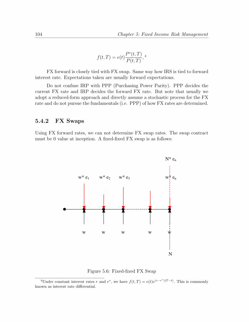
104 Chapter 5: Fixed Income Risk Management
f(t, T ) = e(t)P ∗(t, T )
P (t, T ), 4
FX forward is closely tied with FX swap. Same way how IRS is tied to forwardinterest rate. Expectations taken are usually forward expectations.
Do not confuse IRP with PPP (Purchasing Power Parity). PPP decides thecurrent FX rate and IRP decides the forward FX rate. But note that usually weadopt a reduced-form approach and directly assume a stochastic process for the FXrate and do not pursue the fundamentals (i.e. PPP) of how FX rates are determined.
5.4.2 FX Swaps
Using FX forward rates, we can not determine FX swap rates. The swap contractmust be 0 value at inception. A fixed-fixed FX swap is as follows:
w w w w
w* e1
w
w* e2 w* e3 w* en
N* en
N
Figure 5.6: Fixed-fixed FX Swap
4Under constant interest rates r and r∗, we have f(t, T ) = e(t)e(r−r∗)(T−t). This is commonly
known as interest rate differential.

FX Risk Management 105
Hence, traders must set w and w∗ in such a way that the following holds:
0 =∑n
i=1P (t, Ti) (w∗tN
∗E[e(Ti)]− wtN) + P (t, Tn) (N∗E[e(Tn)]−N)
where N is notional in domestic currency and N∗ is notional in foreign currency,similarly wt and w∗t are domestic fixed and foreign fixed rates respectively. Usuallynotionals are set by (N∗e(t)−N) = 0.
It turns out that (known as the forward expectation – see the Appendix for abrief discussion of the forward expectation):
Et[e(Ti)] = f(t, Ti)
which is the forward FX rate. Then:
∑n
i=1P (t, Ti) (w∗0N
∗f(t, Ti)− w0N) + P (t, Tn) (N∗f(t, Tn)−N) = 0
w0N = w∗0N∗∑n
i=1 P (t, Ti)f(t, Ti)∑ni=1 P (t, Ti)
+P (t, Tn) (N∗f(t, Tn)−N)∑n
i=1 P (t, Ti)
We can see that ifN∗f(t, Tn) = N , then the relative fixed rates, i.e. w0N/w∗0N∗,
are set as in IRS which is the weighted average of forward FX rates.
An Example – Fixed-Fixed FX Swap
A fixed-fixed FX swap is £100 for $150 as the current exchange rate is 1:1.5 (e0 =1.5). In each country the interest rate is 5% (w∗0 = w0). Note that
N∗e0 −N = £100× 1.5− $150 = 0
as the initial condition. The exchange of the currencies is 5 for $7.5 annually.
The actual cash flows (cash flows are fixed but exchange rates are random)are:
∑n
i=1(w∗0N
∗ei − w0N0)P1,Ti + (N∗en −N0)P1,Tn
One year later the exchange rate changes to 1:2 (e1 = 2). Then a new FXswap will be 5 for $10. In this case, N1 = e1N
∗ = $200. In this case, we can do areverse swap:

106 Chapter 5: Fixed Income Risk Management
−∑n
i=2(w∗0N
∗ei − w0N1)P2,Ti + (N∗en −N1)P2,Tn
which will cancel the previous swap on the pound leg and lead to the following net:
V1 =∑n
i=2w0(N1 −N0)P2,Ti + (N1 −N0)P2,Tn
=∑n
i=2w0(e1N
∗ − e0N∗)P2,Ti + (e1N
∗ − e0N∗)P2,Tn
= N∗∑n
i=2w0(e1 − e0)P2,Ti + (e1 − e0)P2,Tn
init 150 100 1.5
dollar leg pound leg ex rate
0
1 -7.5 5 200 100 2
2 -7.5 5 10 -5 2.5 0
3 -7.5 5 10 -5 2.5 0
4 -7.5 5 10 -5 2.5 0
5 -7.5 5 10 -5 2.5 0
6 -7.5 5 10 -5 2.5 0
7 -7.5 5 10 -5 2.5 0
8 -7.5 5 10 -5 2.5 0
9 -7.5 5 10 -5 2.5 0
10 -157.5 105 210 -105 52.5 0
yield 5% 5% 5% 5%
Figure 5.7: Same w
Fixed-Floating FX Swap
A fixed-floating FX swap is more popular but more complex as it involves bothrandom exchange rates and random foreign interest rates. Using the same derivationas in fixed-fixed, we have:

FX Risk Management 107
init 150 100 1.5
dollar leg pound leg ex rate
0
1 -12 5 150 100 1.5
2 -12 5 15 -5 3 0
3 -12 5 15 -5 3 0
4 -12 5 15 -5 3 0
5 -12 5 15 -5 3 0
6 -12 5 15 -5 3 0
7 -12 5 15 -5 3 0
8 -12 5 15 -5 3 0
9 -12 5 15 -5 3 0
10 -162 105 165 -105 3 0
yield 8% 5% 10% 5%
Figure 5.8: Different w and w*

108 Chapter 5: Fixed Income Risk Management
Et[∑n
i=1Λ(t, Ti) (x∗iN
∗ei − w0N) + Λ(t, Tn) (N∗en −N)]
=∑n
i=1P (t, Ti)
(N∗E(i)
t [x∗i ei]− w0N)
+ P (t, Tn)(N∗E(n)
t [en]−N)
= 0
where Et is risk-neutral expectation and Et is forward expectation.
But now we have to deal with the covariance between x∗i and ei. This is knownas the “quanto” effect in FX analyses. We shall discuss this effect later. Note that ifthe foreign interest rates (i.e. x∗) and the exchange rate (i.e. e) are not correlated,then the expectation can be separated, and then there is no quanto effect. Hence,quanto is a result of correlation between x∗ and e.
To avoid the problem, we keep all foreign cash flows in the foreign country andonly discount them once:
e0E∗t[∑n
i=1Λ∗(t, Ti)x
∗iN∗ + Λ∗(t, Tn)N∗
]− Et
[∑n
i=1Λ(t, Ti) (w0N) + Λ(t, Tn) (N)
]= 0
e0
[∑n
i=1P ∗(t, Ti)f
∗i + P ∗(t, Tn)
]N∗ −
[∑n
i=1P (t, Ti)w0 + P (t, Tn)
]N = 0
w0 =1∑n
i=1 P (t, Ti)
e0
∑n
i=1P ∗(t, Ti)f
∗i + [e0P
∗(t, Tn)N∗ − P (t, Tn)N ]
This way, we by pass the quanto issue.
Floating-Floating FX Swap
Usually there is a fixed spread on one of the sides of the swap so that the swapcontract has 0 value. If no spread is specified, then it is known as the differentialswap (or diff swap) and in such cases there WILL BE a cash amount exchanged atinception.
Et[∑n
i=1Λ(t, Ti) (x∗iN
∗ei − (xi + s)N) + Λ(t, Tn) (N∗en −N)]
=∑n
i=1P (t, Ti)
(N∗E(i)
t [x∗i ei]− (E(i)t [xi] + s)N
)+ P (t, Tn)
(N∗E(n)
t [en]−N)
= 0
This is too complicated. So we will not convert till end.
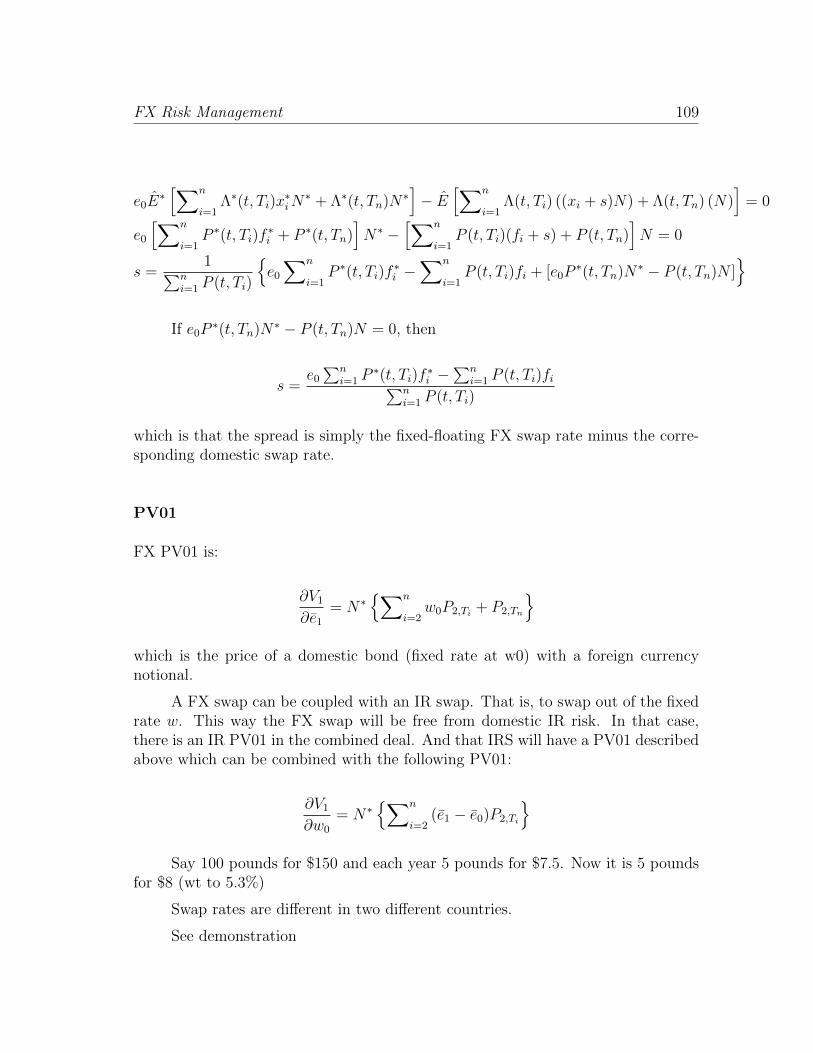
FX Risk Management 109
e0E∗[∑n
i=1Λ∗(t, Ti)x
∗iN∗ + Λ∗(t, Tn)N∗
]− E
[∑n
i=1Λ(t, Ti) ((xi + s)N) + Λ(t, Tn) (N)
]= 0
e0
[∑n
i=1P ∗(t, Ti)f
∗i + P ∗(t, Tn)
]N∗ −
[∑n
i=1P (t, Ti)(fi + s) + P (t, Tn)
]N = 0
s =1∑n
i=1 P (t, Ti)
e0
∑n
i=1P ∗(t, Ti)f
∗i −
∑n
i=1P (t, Ti)fi + [e0P
∗(t, Tn)N∗ − P (t, Tn)N ]
If e0P∗(t, Tn)N∗ − P (t, Tn)N = 0, then
s =e0
∑ni=1 P
∗(t, Ti)f∗i −
∑ni=1 P (t, Ti)fi∑n
i=1 P (t, Ti)
which is that the spread is simply the fixed-floating FX swap rate minus the corre-sponding domestic swap rate.
PV01
FX PV01 is:
∂V1
∂e1
= N∗∑n
i=2w0P2,Ti + P2,Tn
which is the price of a domestic bond (fixed rate at w0) with a foreign currencynotional.
A FX swap can be coupled with an IR swap. That is, to swap out of the fixedrate w. This way the FX swap will be free from domestic IR risk. In that case,there is an IR PV01 in the combined deal. And that IRS will have a PV01 describedabove which can be combined with the following PV01:
∂V1
∂w0
= N∗∑n
i=2(e1 − e0)P2,Ti
Say 100 pounds for $150 and each year 5 pounds for $7.5. Now it is 5 pounds
for $8 (wt to 5.3%)
Swap rates are different in two different countries.
See demonstration

110 Chapter 5: Fixed Income Risk Management
5.4.3 Quanto
The quanto effect exists when the exchange rate and the two interest rates are allrandom and correlated. To see this more clearly, we use the Nikkei option5 as anexample.
Define a “variable rate” call option that pays maxS∗T − K, 0 in yen. Thenin dollars, it is YT maxS∗T −K, 0 at time T . Now we can simply discount it backat the domestic rate r:
C∗t = e−r(T−t)Et[YT maxS∗T −K, 0]= e−r(T−t)e(r−r∗)(T−t)YtE(Y )
t [maxS∗T −K, 0]= e−r
∗(T−t)Yt[er∗(T−t)S∗tN(d+)−KN(d−)
]= Yt
[S∗tN(d+)− e−r∗(T−t)KN(d−)
] (5.11)
where
d± =lnS∗t − lnK + (r∗ ± 1/2v∗)(T − t)√
v∗(T − t)
and hence there is no quanto effect in the option price.
Define a “fixed rate” call that pays Y maxS∗T −K, 0. Then,
Ct = e−r(T−t)Y Et[maxS∗T −K, 0]= e−r
∗(T−t)Y[e(r∗+ρσY v
∗)(T−t)S∗tN(d+)−KN(d−)] (5.12)
where
d± =lnS∗t − lnK + (r∗ ± 1/2v∗2)(T − t)
v∗√T − t
and hence the quanto effect exists.
5.4.4 FX Option Formula
Consider the interest rate parity theorem and a simple Black-Scholes type model:
de
e= (r − r∗)dt+ σdWe
dr = κ(θ − r)dt+ γdW
dr∗ = κ∗(θ∗ − r∗)dt+ γ∗dW ∗
5The Nikkei index put option is ...

FX Risk Management 111
and dWidWj = ρijdt and i, j = e, r, ∗. The IRP theorem restricts the drift of theexchange rate to be the difference between the two rates. (Note alternatively wecan view the foreign interest rate as a “dividend” that takes away the return frominvesting in the domestic risk-free bond.)
We also modify the Black-Scholes option formula as follows:
Ct = P ∗t,T etN(d1)− Pt,TKN(d2)
where
d1 =ln et − lnK − lnPt,T + lnP ∗t,T + v2/2
√v
d2 = d1 − v√T − t
v2 = var[ln eT − lnDt,T + lnD∗t,T ]
Dt,T = exp
−∫ T
t
rudu
D∗t,T = exp
−∫ T
t
r∗udu
5.4.5 FX Basis
An FX basis is the discrepancy between the IRP and actual IR differential. In otherwords, an FX basis is where the market disagrees with the theory. In theory therewill exist arbitrage profits but due to market frictions, such profits are too small tobe worth taking.
One key aspect of FX bases is that they are random. This adds an additionalrisk to consider and hedge/manage.
5.4.6 FX models
First we review the Black-Scholes model. In the case of stocks, we have:
dS
S= (µ− `)dt+ σdW (5.13)
where µ is the expected return of the stock and ` is the (continuous) dividend yield.6
In a general case, d can be regarded as any leakage of return from the underlying
6We note that under discrete dollar dividends, the model is quite different.

112 Chapter 5: Fixed Income Risk Management
asset. In the case of FX, it is the foreign risk-free rate; in the case of real estate, itis rent; in the case of commodities, it is convenience yield; and finally in the case offutures, it is risk-free rate itself.
The FX rates are also modeled the same way as (5.13):
dX
X= (rD − rF )dt+ σdW (5.14)
where rD and rF are domestic and foreign risk-free rates respectively. Comparedwith equation (5.13), the above equation substitutes rD for µ and rF for `. Thisresult is a consequence of what is known as the interest parity theorem. An investorcan choose to put his or her money in a domestic risk-free account (making thedomestic risk-free return) or a foreign risk-free account (making the foreign risk-freereturn). Since the investor can only choose one or the other, by choosing one, he orshe has to let go of the other. For the domestic point of view, the foreign risk-freereturn is a “leak”.
Another way to look at this is the notion of opportunity cost. By investingdomestically, a foreign opportunity is let go and hence it must be considered as aloss (just like dividends) to the “return” on the exchange rate. Such a notion isapplied repeatedly in other asset classes (convenience yield in commodities and rentin real estate).
The FX option (e.g. call) hence is evaluated similar to the Black-Scholesformula as in equity as follows:
Ct = e−rF (T−t)XtN(d1)− e−rD(T−t)KN(d2) (5.15)
The binomial model needs to be modified as shown in Figure 5.9.
0X
11 0X uX=
10 0X dX=
Figure 5.9: Binomial Model for the FX Rate
where the probabilities are modified as:
p =e(rD−rF )∆t − d
u− d(5.16)

Total Return Swap 113
and rD and rF are domestic and foreign risk-free rates respectively.
5.5 Total Return Swap
A total return swap (TRS) is usually a floating-floating swap, or diff swap. A typicalexample is a swap between an equity index (e.g. S&P 500) and an interest rate index(e.g. LIBOR). As in any diff swap, there is a spread on the IR leg.
Another popular TRS can be a real estate index (e.g. NCREIF) for an IRindex.
5.6 Residential Mortgage
Residential mortgages (usually refer to Prime mortgages) are guaranteed by govern-ment agencies known as GNMA (Ginnie Mae), FNMA (Fannie Mae), and FHLMC(Freddie Mac).78
Residential mortgages are exposed to prepayment risk. Prepayment is an ac-tion taken by mortgage borrowers to pay pre-maturely full or partial amount of theloan. Prepayments affect the incomes of the lenders. Simply speaking, prepaymentsreduce the loan amounts and hence reduce the interests earned by the lenders. Asa result, prepayments represent a risk. However, not all prepayments are bad news.When prepayments occur in a time when interest rates are high, then banks can loanout the early payment amounts at a higher rate and make more interest incomes.On the contrary, when prepayments occur in a time when interest rates are low,banks directly lose interest earnings.
If the reason of a prepayment is non-economical, such as divorce, job change,addition to family, then prepayments can be either good or bad news. However, if aprepayment is due to re-finance of the mortgage, then it is surely bad for the bank.Hence, the models for mortgages are categorized into two big areas: prepaymentand refinance.
7They are Government National Mortgage Association, Federal National Mortgage Association,and Federal Home Loan Mortgage Corporation respectively.
8Note that there are a small number of residential mortgages that are not guaranteed by thethree agencies. These mortgages are not included in this section.

114 Chapter 5: Fixed Income Risk Management
5.6.1 Refinance Modeling
Refinancing is a decision directly linked to mortgage rates, which in turn related toTreasury interest rates (most commonly the 10-year rate). As rates drop, borrowerssubstitute new mortgages that have lower mortgage rates for existing mortgages thathave higher mortgage rates. And as borrowers refinance, banks lose future interestrevenues. In other words, the values of mortgages that banks make decrease.
As refinancing is a predictable event that happens when rates drop, we canthen run an interest rate model to forecast and gauge the impacts of future ratedrops. Then the impacts can be factored into today mortgage rate. For example,if rates are expected to fall and refinancing is highly expected, then banks shouldcharge a higher mortgage rate to compensate for the future loss. Figure 5.10 demon-strates how refinance actions are modeled in an interest rate model. As Figure 5.10demonstrates, the lower part of the model is the refinance area as rates are low.
low rates and refi likely
Figure 5.10: An Interest Rate Model
5.6.2 Prepayment Modeling
Prepayment is usually modeled with some kind of “response function” which isgraphically similar to an “S” curve. An “S” function is bounded between 0 and 1and can be modeled via a number of different functional forms such as arc-tangent,logit, and probit. In the mortgage area, the logit function is the most popular

Residential Mortgage 115
choice.9
The logit function is:
p =exp(α +
∑βkxk)
1 + exp(α +∑βkxk)
(5.17)
where the dependent variable p is the prepayment rate and the explanatory variablesare chosen as follows.
• Housing Turnover Rate (When a house is bought and sold, the existing mort-gage is usually prepaid completely and a new mortgage is taken (unless theexisting mortgage is assumable). As a result, higher turnover rates for a par-ticular housing sector implies higher prepayment rate and hence higher risk forinvestors. For example, apartments are turned over faster then single homes.)
• Seasonality (Housing markets present seasonality – more people are buyinghomes in summer than in winter. As mentioned above, housing turnover isdirectly linked to prepayment. Hence summer prepayment rate is higher thanthat in winter.)
• Cash-out (This is how much cash is left in the mortgage. As the propertyappreciates, the difference between house value and mortgage gets larger, andthe cash-out effect becomes stronger.)
• Refinance (This is to be discussed separately later. Basically, refinance occursin low interest rate times.)
• Age (This is the age of the mortgage, not the age of the borrower. The age ofa mortgage has a negative impact of prepayment. In other words, the longera homeowner holds on to the mortgage, the less likely he or she will prepayearly.)
• Burnout (In a mortgage-backed security, the percentage of mortgages under-lying the security that were not re-financed following a drop in interest rates.Historically, a mortgage that is not re-financed is less likely to re-finance at thenext drop in interest rates. As a result, potential investors in mortgage-backedsecurities often look for a high burnout rate because it reduces prepaymentrisk, or the risk that investors will be deprived of future interest paymentsbecause too many mortgages are prepaid.)
9OTS, or Office of Thrift Supervision, used to use an arc-tangent function for prepayment butit was dissolved in 2011.

116 Chapter 5: Fixed Income Risk Management
• Yield Curve (Interest rates have the most impacts on prepayments (or refi-nance).)
• Equity (As monthly payments are made, the equity of the house increases.The homeowner now can borrow more now as the LTV improves.)
• Credit (As mortgage is paid off gradually (FRM), credit is improved as LTVis improved.)
• Curtailment (As opposed to prepayment that pays off the mortgage in entirety,a curtailment is to pay more than the required monthly payment. Hence, theeffect of curtailments is similar to (but milder than) that of prepayment.)
The most common measure of prepayment speed is SMM (single month mor-tality) rate. SMM is used in interest rate models to evaluate mortgages. SMM isestimated empirically using the above factors. In other words, SMM is the dependentvariable (think of a regression) and the above factors are independent (explanatory)variables. The function used is a response function. The usual shape of a responsefunction is an S curve bounded between 0 and 1. Logit or probit functions (bothbounded between 0 and 1) are also plausible functions used for estimating SMM.Arc-tangent functions can be used as well.
The other two measures used in practice are:
• PSA (Public Securities Association) Standards
• CPR (constant prepayment rate)
These are measures of the speed of prepayment and not models of prepayment.However, by monitoring these measures one can gain a sense of how the prepaymentbehavior. Models of prepayment can be found in many fixed income textbooks.
5.6.3 Default Modeling
Since prime residential mortgages are usually underwritten by the Agencies, theyare default-protected by the Agencies. This is the credit-enhancement provided bythe Agencies so that investors do not need to worry about defaults. This is oneof the major functions the Agencies provide in order to facilitate secondary markettrading.
While defaults are not a concern in residential mortgages, they are a trueconcern for commercial mortgages. Since commercial mortgages are not protectedby the Agencies, they are subject to default risk.

Combined with Other Assets 117
However, commercial mortgages do not suffer from prepayment risk in thatall commercial loans have a “yield maintenance” clause which protects investors byhaving a guaranteed yield for a certain period (hence yield is “maintained”). In otherwords, there is a heavy prepayment penalty which is so high that borrowers haveno incentive to prepay. The period under protection is called the yield maintenanceperiod (or YM period)
5.6.4 OAS – Option Adjusted Spread
Spread01 or Spread PV01.
5.7 Combined with Other Assets
How do we compute IR risk for a portfolio of stocks and bonds. Stocks are affectedby interest rates but there are no clean models (both are “primary assets”). Thecommon practice is to run regression (one could do PCA but then each PC must beinvestigated to see if it is sensitive to interest rates) of stock on rates.
dS = b0 +∑K
k=1bkrk + · · ·+ e
Then, dS/drk = bk can be used in the portfolio VaR calculation.
A portfolio of a call and a bond. The call option must be evaluated with theRabinovitch model (1989) which takes into account of random interest rates. Thenwe have
dV = nCdC + n2dP
= n1mC + n2mP
where
mC = CSdS + 1/2CSSdS2 + Ctdt+ Crdr + 1/2Crrdr
2 + CSrdSdr
and
mP = Prdr + 1/2Prrdr2 + Ptdt
Then

118 Chapter 5: Fixed Income Risk Management
var[dV ] = n2C var[mC ] + n2
P var[mP ] + 2nCnP cov[mC ,mP ]
= n2C
C2S var[dS] + C2
r var[dr] + 2CSCr cov[dS, dr]
+ n2PP
2r var[dr]
+ 2nCnP CSPr cov[dS, dr] + CrPr var[dr]
A convertible bond is another good example. A CB is exposed to three im-portant risks – equity (convert), interest rate (coupons and principal), and credit(default). A convertible bond can be expressed as:
B =
maxΠ, ξS if survives
R if defaults
5.8 Appendix
5.8.1 FX Swap Curve and Fixed-Fixed FX Swaps
If we already know the coupons of domestic and foreign bonds, then we can solvefor the FX swap rate as follows.
V0 = 0 =∑
(w∗0N∗e0 − w0N)P0,Ti + (N∗e0 −N)P0,Tn
=∑
(w∗0N∗e0 − w0N
∗e0)P0,Ti + (N∗e0 −N∗e0)P0,Tn
= N∗∑
(w∗0 e0 − w0e0)P0,Ti + (e0 − e0)P0,Tn
The job is to solve for the FX swap rate. It is clear that the FX swap rate canbe solved the same way as the IR swap rate.
∑n
i=1w0e0P0,Ti + e0P0,Tn = e0
∑n
i=1w∗0P0,Ti + P0,Tn
e0 =
∑ni=1w0e0P0,Ti + e0P0,Tn∑ni=1w
∗0P0,Ti + P0,Tn
where the similarity remains. However, note that this is not to contradict the resultin the text where we solve for the relative coupon rates using the FX forward curve.

Appendix 119
5.8.2 Commodities and Real Assets
Some times commodities are included in the category of fixed income and so namedFICC (Fixed Income, Currencies and Commodities), although the risk characteris-tics of commodities are quite different from IR and FX.
Commodities are very difficult to price and also their derivatives. Unlike fi-nancial assets, commodities (or real assets) are:
• difficult to transact (hence liquidity is very low)
• require large storage cost (including funding cost)
• usually present cycles (including seasonality)
In commodities, two popular terminologies should be paid attention to:
• contango
• backwardation
Contango is defined as the futures price greater than the spot price: Φ(t, T ) >S(t) where T is the settlement date. This is a normal situation as storage costis high. For a buyer who wants a commodity in the future, he can either buyfutures contracts, or he can buy spot and store it, whichever is cheaper. As a result,Φ(t, T ) = S(t) + C(t, T ) > S(t).
Backwardation is defined as the futures price smaller than the spot price:Φ(t, T ) < S(t). Under the phenomenon of cost of carry, this is not possible asarbitrageurs of such commodities will just buy futures and sell short the spot to makeprofits. Hence the only logical explanation of backwardation existing must be thatshort-selling commodities is prohibitedly costly. Such a cost is termed convenienceyield.
Convenience yield happens (i.e. backwardation) when the spot is very rareand hence short-selling is difficult. To short sell, the seller must borrow the spot.When the spot is rare, then the cost of borrowing is consequently high. There aretwo kinds of rareness. The first is physical, which means the commodity is simplynot available. For example, during winter, agriculture products (e.g. corn) are rare,as farmlands cannot produce. Hence to borrow corn to short must pay a higherprice. The other kind is the spot is in high demand and its price is skyrocketing.Under this situation, the borrower must pay for the expected growth in price as partof the borrowing cost. For example, gold (or precious metals) is very expensive toborrow during a recession as everyone buys gold to hedge a recession.

120 Chapter 5: Fixed Income Risk Management
As we can see, convenience yield shares the same flavor as seasonality as spotprices of commodities can present cyclical patterns repeatedly. As the two examplesearlier, agricultural products present price cycles within a year (seasonality) andprecious metals present price cycles along with recessions. Should commodities beabsolutely liquid, such cycles cannot exist as one can buy and sell these goods easilyat no cost.
By now, we can understand the classical financial models cannot be appliedeasily to commodities. All financial models assume perfect liquidity that rules outcyclicality and seasonality. However, convenience yield can be regarded as leakage ofthe spot because it represents the cost of hold the spot. This is similar to dividendsof stocks, or foreign interest returns of exchange rates.
Equation (5.13) is then used as the best approximation to model commodities.Eduardo Schwartz (1979) uses equation (5.13) with a mean-reverting convenienceyield process:
dS
S= (µ− `)dt+ σdW1
d` = κ(θ − `)dt+ γdW2
(5.18)
where ` represents “convenience yield” and dW1dW2 = ρdt. The convenience yieldhere now can be either positive or negative. When it is substantially negative (largerthan µ so µ− ` < 0), then the futures price will be smaller than the spot price andwe have a backwardation. If ` is negative, then it is similar to having a contango.Given that ` is normally distributed, there is a closed-form solution to the futuresprice (and futures option):
Φ(t, T ) = E[ST ] = exp
E[lnST ] +
1
2V[lnST ]
where
E[lnST ] = lnSt + (µ− 12σ2)(T − t)−
[`t
1
κ
(e−κ(T−t) − 1
)+ θ
(T − t− 1
κ
(e−κ(T−t) − 1
))]V[lnST ] =
γ2
2κ
(e2κ(T−t) − 1
)+ σ2(T − t) +
2ργσ
κ
(eκ(T−t − 1
)Another important pricing question related to commodities (and not so much
for financial assets) is the level of inventory. As storing commodities suffers (enjoys)high storage costs (convenience yield), how much to store (level of inventory) is animportant decision. William J. Baumol (1952) has a simple model to explain the

Appendix 121
demand for inventory.10 Say farmers hold Q bushels of wheat of which Q1 to besold at time T1 and Q2 to be sold at time T2. P1 and P2 are prices respectively. IfP1 > PV[P2], then farmers will sell all Q at T1.
A marketing cost is assumed as ξQ2. Also PV[P2] = DP2. So the total revenuefrom both sales is (P1Q1 − ξQ2
1) + D(P2Q2 − ξQ22). Maximizing the total revenue
leads to (substituting Q − Q2 for Q1 and taking first order derivative with respectto Q2):
−P1 + 2ξ(Q−Q2) +D(P2 − 2ξQ2) = 0
and the optimal solution for Q2 is:
Q2 =DP2 − P1 + 2ξQ
2ξ(1 +D)
which implies a positive inventory (i.e. Q2 > 0) if:
DP2 − P1 > −2ξQ
that is the price differential must be larger enough to justify an inventory. Thelarger is the price in the second sale (P2), the higher is the inventory level (Q2).This is known as the transaction demand for inventory.
A second theory for inventory is known as the precautionary demand for in-ventory (S. C. Tsiang, 1969).11 Let z be amount arrived; I precautionary stock; xa unit loss from the shortage; K demand; and c cost of holding an inventory.12
If z is too low to operate at full capacity, then the firm will suffer a shortagecost:
(K − I − z)x
Expected shortage cost:∫ K−I
0
(K − I − z)xf(z)dz
10William J. Baumol, The Quarterly Journal of Economics, Vol. 66, No. 4 (Nov., 1952), pp.545-556.
11S. C. Tsiang, Journal of Political Economy, Vol. 77, No. 1 (Jan. - Feb., 1969).12The following derivation is taken from The Economic Function of Futures MarketsOct 27, 1989
by Jeffrey C. Williams.

122 Chapter 5: Fixed Income Risk Management
Cost of precautionary inventory is Ic so the total cost is:
Ic+
∫ K−I
0
(K − I − z)xf(z)dz
Optimal level of inventory I∗ is:
c−∫ K−I∗
0
xf(z)dz = 0
The higher is storage cost c, the less should be the inventory (i.e. I∗ is smallerand K−I∗ is larger). The higher is the opportunity cost x, the lower is the inventory.
Real estate is another real asset that follows the same model. In investing inreal estate, the buyer now needs not to rent and therefore return on the propertymust be reduced by the amount of rent. Now ` represents the percentage rent.Another way to look at this is that the buyer buys the property for purely rentalpurposes. He or she spends the money and expects to gain returns on the investment.Rental incomes therefore must be a part of the total (cum) return. Given that rentsare collected (leaked out) in cash, it must be deducted from the total return.
One thing particular to the real estate market is that properties need to bedepreciated. As a result, the minimum return for the property to generate is the de-preciate rate. Because of this, the convenience yield now ` is rent minus depreciationrate.

Appendix 123
0.0
001
0.0
001
0.0
001
0.0
001
0.0
001
0.0
001
0.0
001
0.0
001
0.0
001
0.0
001
10.0
89432
0.9
1791
0.0
89532
0.9
17825
0.0
89432
0.9
1791
0.0
89432
0.9
1791
0.0
89432
0.9
1791
0.0
89432
0.9
1791
0.0
89532
0.9
17825
20.0
92061
0.8
38506
0.0
92061
0.8
38506
0.0
92161
0.8
38353
0.0
92061
0.8
38506
0.0
92061
0.8
38506
0.0
92061
0.8
38506
0.0
92161
0.8
38353
30.0
50936
0.8
61533
0.0
50936
0.8
61533
0.0
50936
0.8
61533
0.0
51036
0.8
61287
0.0
50936
0.8
61533
0.0
50936
0.8
61533
0.0
51036
0.8
61287
40.0
59417
0.7
93838
0.0
59417
0.7
93838
0.0
59417
0.7
93838
0.0
59417
0.7
93838
0.0
59517
0.7
93539
0.0
59417
0.7
93838
0.0
59517
0.7
93539
50.0
57017
0.7
5786
0.0
57017
0.7
5786
0.0
57017
0.7
5786
0.0
57017
0.7
5786
0.0
57017
0.7
5786
0.0
57117
0.7
57502
0.0
57117
0.7
57502
0.9
66343
0.9
66339
0.9
66335
0.9
6633
0.9
66328
0.9
65966
0.9
65927
0.0
42124
0.0
76771
0.1
22943
0.1
49828
3.7
63077
4.1
54744
0.0
001
0.0
001
0.0
0005
0.0
0005
0.0
001
0.0
001
0.0
001
0.0
0005
0.0
0005
0.0
001
0.0
001
0.0
001
10.0
89432
0.9
1791
0.0
89532
0.9
17825
0.0
89432
0.9
1791
0.0
89432
0.9
1791
0.0
89432
0.9
1791
0.0
89432
0.9
1791
0.0
89532
0.9
17825
20.0
92061
0.8
38506
0.0
92111
0.8
38429
0.0
92061
0.8
38506
0.0
92111
0.8
38429
0.0
92061
0.8
38506
0.0
92061
0.8
38506
0.0
92161
0.8
38353
30.0
50936
0.8
61533
0.0
50936
0.8
61533
0.0
50936
0.8
61533
0.0
51036
0.8
61287
0.0
50936
0.8
61533
0.0
50936
0.8
61533
0.0
51036
0.8
61287
40.0
59417
0.7
93838
0.0
59417
0.7
93838
0.0
59417
0.7
93838
0.0
59467
0.7
93688
0.0
59417
0.7
93838
0.0
59467
0.7
93688
0.0
59517
0.7
93539
50.0
57017
0.7
5786
0.0
57017
0.7
5786
0.0
57017
0.7
5786
0.0
57017
0.7
5786
0.0
57017
0.7
5786
0.0
57117
0.7
57502
0.0
57117
0.7
57502
0.9
66343
0.9
66335
0.9
66343
0.9
66319
0.9
66343
0.9
65959
0.9
65927
0.0
80512
00.2
36254
03.8
38
4.1
54744
Fig
ure
5.11
:T
rian
gula
rR
ule
for
Key
Rat
eD
ura
tion

124 Chapter 5: Fixed Income Risk Management

Chapter 6
P&L Attribution
6.1 Introduction
The P&L attribution is to explain where the profits and losses come from. Due tothe fact that luck plays a critical role in trading, managers need to make sure thattheir traders make money not due to luck but due to skills (or talents). As a result,P&L attribution has become essential in trading and fund management business.
6.2 Taylor’s Series Expansion and Explanatory Risk
Factors
Greeks are key to explain relative importance of each risk factor. We define thebasic Greeks as follows:
∆ = ∂C∂S
= partial derivative of target (e.g. call) with respective to the under-lying (e.g. stock)
V = ∂C∂σ
= partial derivative of target (e.g. call) with respective to the volatility
P = ∂C∂r
= partial derivative of target (e.g. call) with respective to the theinterest rate
Θ = ∂C∂t
= partial derivative of target (e.g. call) with respective to time (knownas time decay)
Γ = ∂2C∂S2 = partial derivative of target (e.g. call) twice with respective to the
underlying
Cross Greeks can be defined, as a few examples, as follows:

126 Chapter 6: P&L Attribution
∆V = V ∆ =∂2C
∂S∂σ(Vanna)
ΓV =∂2C
∂σ∂σ(Volga)
∆P = P∆ =∂2C
∂S∂r
PV = V P =∂2C
∂r∂σ
where the first two are popular in FX.
Take a single product as an example (e.g. call option). The explanatory factorsare price, volatility, and time which translate to Delta, Gamma, Vega, and Theta.If the BS model is the correct model, then we know that:
dC =(µSCS + σ2S2CSS + Ct
)dt+ σSCSdW
=(µS∆ + σ2S2Γ + Θ
)︸ ︷︷ ︸explanatory factors
dt+ σS∆dW︸ ︷︷ ︸unexplained
(6.1)
and there is no Vega. If the volatility and the risk-free rate are both random, thenwe must first define the volatility and interest rate processes. Usually we write bothof them as mean-reverting square root processes:
dS = µSdt+√V SdW1
dV = α(β − V )dt+√V γdW2
dr = a(b− r)dt+√rgdW3
(6.2)
where dWidWj = ρijdt. Then the P&L attribution becomes:

Pictorial P&L Attribution 127
dC = CSdS + CV dV + Crdr + CSS(dS)2 + CV V (dV )2 + Crr(dr)2
+ CSV (dS)(dV ) + CSr(dS)(dr) + CV r(dV )(dr) + Ct
=
[µSCS + α(β − V )CV + a(b− r)Cr + Ct+
V S2CSS + γ2V CV V + g2rCrr + V Sγρ12CSV + rSgρ13CSr +√rV γgρ23CV r
]dt
+√V SCSdW1 + σ
√V CV dW2 + g
√rPdW3
=
[µS∆ + α(β − V )V + a(b− r)P + Θ+
V S2Γ + γ2V V V + g2rPP + V Sγρ12∆V + rSgρ13∆P +√rV γgρ23V P
]︸ ︷︷ ︸
explanatory factors
dt
+√V S∆dW1 + γ
√V V dW2 + g
√rPdW3︸ ︷︷ ︸
unexplained
(6.3)
As we can see, the model can expand to as many random factors as we wish. Asshown in the exhibit earlier, the random factors can include FX, multiple key interestrates, credit, prepayment, and any other risk factors. At the end, the equation canbe very long and the number of parameters can become quite unimaginable. Somesimplifications must be necessary.
The first simplification is as easy as just ignoring higher order (and cross)Greeks. We can assume that higher order Greeks such as Vega-Vega and Delta-Vega effects are small and ignore them. The second simplification is to adopt theVaR methodology and choose several key benchmark indices.
6.3 Pictorial P&L Attribution
Figure 6.1 is taken from http://www.pnlexplained.com/ on 12/15/2009 which de-scribes very well the concept of P&L attribution.
At the bottom layer, we see various first order Greeks such as Delta and Vega,and various higher order Greeks such as Gamma and cross Greeks (cross Gammaand Vega-Gamma).

128 Chapter 6: P&L Attribution
Figure 6.1: P&L Decomposition

Chapter 7
Value Adjustment
7.1 VA – Value Adjustment
As previously discussed, valuation is important in providing reliable risk manage-ment. This is particularly so when there are no liquidly observable prices. Whenprices are not always observable, models are used to estimate those prices. Modelsmake assumptions about the connections between observables in the market place(inputs to the model) to the prices and risk metrics (outputs of the model) of theassets. Complex models are believe to generate more accurate estimates for pricesbut require a comprehensive set of inputs and often need a long time to computeprices and risk metrics. As a result, these models cannot be used for day-to-day riskmanagement. Simpler models are therefore developed to quickly estimate pricesfor day-to-day risk management but these estimates can be inaccurate. To balancebetween the two, a concept of VA (value adjustment) is adopted by the industry.
The idea of a VA is to run simple models every day but periodically checkagainst more comprehensive models. In other words, simple models are “calibrate”to more complex models on a less frequent basis and then run on their own untilthe next calibration. This constant process of re-calibration has its own become animportant methodology which needs to be validated to insure the “calibration” eachtime is done properly. The complex models themselves are subject to extra scrutinyto insure absolute accuracy in providing proper valuation.
The complex models need to validated thoroughly. This always requires care-fully designed econometric methods for parameter estimation (see later), compre-hensive back tests and stress tests, sensitivity analyses on parameters, and a fullrevelation on model risk.
Take a CDO as an example. There are several simple models currently used

130 Chapter 7: Value Adjustment
such as:
• correlation skew
• binomial diversity score
and yet the full model is done over various stochatic input variables via Monte Carlo(with recursive algorithm and Fourier Inversion).

Chapter 8
Parameter Estimation
8.1 Introduction
To use a model, we must first obtain parameter values. There are two ways toestimate parameter values in a model. One is the reduced-form (familiar with theterm now?) approach and the other is the econometric approach.
The reduced-form approach is to use current market information to “back out”parameter values. The most famous example is the implied volatility of the option,using the Black-Scholes model. One equation (Black-Scholes option pricing formula)and one unknown (volatility). People use the same method to compute parametervalues of other models. For example, we can solve for four parameters of the Vasicekterm structure model using four bonds.
The second method is the econometric method. Historical data are collectedand the full time series behavior of the model is considered. Hence, theoretically, theeconometric method is definitely superior to the reduced-form method. However,given that the parameters are estimated by past prices, hence there is no guaranteethat the model can match the current price. This can be a problem for hedging asthe hedge ratios will then be incorrect.
8.2 Regression estimation for the Vasicek model
Recall that the Vasicek model is a one-factor mean reverting Gaussian model withthe following short rate dynamics
dr = α(µ− r)dt+ σdW (8.1)

132 Chapter 8: Parameter Estimation
under the real measure and the parameters are defined previously. The mean andvariance of r are given as follows:
E[rs|rt] =(1− e−α(s−t))µ+ e−α(s−t)rt (8.2)
and
V[rs|rt] = σ2 1− e−2α(s−t)
2α(8.3)
for s ≥ t.
We know that r is normally distributed. Hence, we can write an AR(1) processin discrete time for r:
rt =(1− e−αh
)µ+ e−αhrt−h + et (8.4)
where h is time interval and et has mean 0 and variance 1−e−2αh
2ασ2. This essentially
an OLS with normally distributed error terms:
rt = a+ brt−h + et (8.5)
with a =(1− e−αh
)µ and b = e−αh. We can then run an OLS to obtain the
parameters. The regression coefficient, b, can be used to estimate α, and then theconstant coefficient, a, can be used for µ. Finally the MSE of the regression modelcan be used to estimate σ. The t statistics of α and µ can be derived from the tstatistics of a and b. With Taylors series expansion, we have:
b ≈ 1− αha ≈ αµh
(8.6)
It then follows that:
var[b] ≈ h2 var[α]
var[a] ≈ (αh)2 var[µ](8.7)
and hence the t statistics can be easily calculated. Finally, the asymptotic standarderror of the SSE of the regression model is 1/(2σ4). Hence, the standard error ofthe MSE is 1/(2Nσ4) where N is the sample size.

Regression estimation for the Vasicek model 133
The problem of the above method is that it fails to estimate the market priceof risk. The chosen interest rate series are regarded as instantaneous rate andhence carries no risk premium. Certainly such a substitution, while convenient andoften times enough to obtain a major intuition of the interest rate dynamics, istheoretically flawed.
To include the market price of risk into the estimation process, we must realizethat any market interest rates are not the instantaneous rate but ”term rates” thatare usually converted to discount factors Pt,T before they can be used for any pricing.In the Vasicek model, this discount factor has a closed-form solution as follows:
Pt,T = e−rtFT−t−GT−t (8.8)
where
FT−t =1− e−α(T−t)
α
GT−t =(µ− σλ
α− σ2
2α2
)(T − t− FT−t) +
σ2F 2T−t
4α2
where λ is the market price of risk. Inverting the pricing formula gives the instan-taneous rate:
rt = − lnPt,T +GT−t
FT−t(8.9)
Note that the above formula must hold regardless of the choice of t. Also notethat at the next period, t+ h, we can write (8.9) as:
rt+h = − lnPt+h,T+h +GT−t
FT−t(8.10)
and the functions F and G remain the same as T + h− (t+ h) = T − t. This resultprovides tremendous convenience in data collection. We can choose CMT (constantmaturity Treasury) rates for the estimation. A 3-month CMT rate have a constantrolling maturity of 3 months. Hence T − t = 1/4. We can use daily (i.e. h = 1/365)CMT rates for estimation.
Substituting (8.9) and (8.10) back into (8.12), we obtain:
− lnPt+h,T+h
T − t=
(1− e−αh
T − t
)(µFT−t +GT−t) + e−αh
− lnPt,TT − t
+FT−tT − t
et (8.11)

134 Chapter 8: Parameter Estimation
An OLS can be performed to arrive at the following estimates:
Slope = e−αh
Intercept =
(1− e−αh
T − t
)(µFT−t +GT−t)
SSE =F 2T−t
(T−t)2σ2(1−e−2αh)
2α
(8.12)
where h is data frequency and T − t is the maturity of the bond. Note that (8.12)has three equations but has four unknowns. The market price of risk contained infunction G cannot be identified. As a result, we must choose another bond seriesand run a simultaneous regression as follows:
− lnPt+h,T+h
T − t=
(1− e−αh
T − t
)(µFT−t +GT−t) + e−αh
− lnPt,TT − t
+FT−tT − t
et
− lnPt+h,T ′+hT ′ − t
=
(1− e−αh
T ′ − t
)(µFT ′−t +GT ′−t) + e−αh
− lnPt,T ′
T ′ − t+FT ′−tT ′ − t
et
(8.13)
where T ′ represents a different maturity. In the simultaneous regression the regres-sors in the two separate equations must be restricted to have the same coefficient.This allows us to solve for a unique set of α, µ, and λ. However, there are two SSEsfrom separate regressions and the choice of σ is arbitrary.
From this exercise, we know that it is impossible to estimate market price ofrisk without crossectional data. A univariate time series data cannot be used toestimate market price of risk.
Finally, via Taylors series expansion, we can derive the standard errors of theparameters:
var[e−αh
]≈ var[1− αh] = h2 var[α]
var
[(1− e−αh
T − t
)(µFT−t +GT−t)
]≈ var
[(1− e−αh
T − t
)[µFT−t +
(µ− σ2
2α2
)(T − t− FT−t) +
σ2F 2T−t
4α
]]=
(1− e−αh
T − t
)2
var [µ(T − t)] =(1− e−αh
)2var[µ]
(8.14)

The Cox-Ingersoll-Ross Model 135
8.3 The Cox-Ingersoll-Ross Model
The CIR model is a one-factor mean-reverting square-root model with the followingshort rate dynamics:
dr = α(µ− r)dt+ σ√rdW (8.15)
under the real measure and the parameters are defined previously. This is a complexdistribution for r. The transition density for r is:
f(rs|rt) = ce−c(rs+ξ)(rsξ
)d/2Id(2c
√rsξ) (8.16)
where
c =2α
σ2 (1− e−α(s−t))
ξ = rte−α(s−t)
d =2αµ
σ2− 1
which after change of variable x = 2cr:
f(xs|xt) =1
2e−
1/2(xs+Λ)(xs
Λ
)d/2Id(√
Λxs) (8.17)
is a non-central chi-square distribution with Λ = 2cξ degrees of non-centrality andυ = 2d + 2 = 4αµ
σ2 degrees of freedom. We know that the mean and variance of anon-central chi-squared distribution are, respectively, υ + Λ and 2(υ + 2Λ), whichlead to (see Chapter ?? for details):
E[rs|rt] =(1− e−α(s−t))µ+ e−α(s−t)rt (8.18)
and
V[rs|rt] =σ2
2α
[(1− e−α(s−t))2
µ+ rt(e−2α(s−t) − e−α(s−t))] (8.19)
It is clear that the mean of r under the CIR model is the same as the meanunder the Vasicek model. However, unlike the Vasicek model, the variance of r isno longer independent of r. As a result, the instantaneous rate r under the CIR
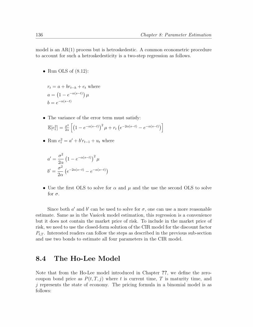
136 Chapter 8: Parameter Estimation
model is an AR(1) process but is hetroskedestic. A common econometric procedureto account for such a hetroskedesticity is a two-step regression as follows.
• Run OLS of (8.12):
rt = a+ brt−h + et where
a =(1− e−α(s−t))µ
b = e−α(s−t)
• The variance of the error term must satisfy:
E[e2t ] = σ2
2α
[(1− e−α(s−t))2
µ+ rt(e−2α(s−t) − e−α(s−t))]
• Run e2t = a′ + b′rt−1 + ut where
a′ =σ2
2α
(1− e−α(s−t))2
µ
b′ =σ2
2α
(e−2α(s−t) − e−α(s−t))
• Use the first OLS to solve for α and µ and the use the second OLS to solvefor σ.
Since both a′ and b′ can be used to solve for σ, one can use a more reasonableestimate. Same as in the Vasicek model estimation, this regression is a conveniencebut it does not contain the market price of risk. To include in the market price ofrisk, we need to use the closed-form solution of the CIR model for the discount factorPt,T . Interested readers can follow the steps as described in the previous sub-sectionand use two bonds to estimate all four parameters in the CIR model.
8.4 The Ho-Lee Model
Note that from the Ho-Lee model introduced in Chapter ??, we define the zero-coupon bond price as P (t, T, j) where t is current time, T is maturity time, andj represents the state of economy. The pricing formula in a binomial model is asfollows:

The Ho-Lee Model 137
P (u, s, j) =
P (t, s, j)
P (t, u, j)d(s− u)
P (u, s, j + 1) =P (t, s, j)
P (t, u, j)u(s− u)
(8.20)
where t < u < s and
u(τ) =1
p+ (1− p)δτ
d(τ) =δτ
p+ (1− p)δτ
The frequency of the data is u−t and the maturity is τ . Note that P (t, s, j)/P (t, u, j)is a forward price. If the yield curve is flat, then P (t, s, j)/P (t, u, j) becomes e−r(s−u)
under state j, which is P (t, t+ s− u, j). Note that this bond has the same time tomaturity as P (u, s, j) or P (u, s, j + 1). As a result, we can write (8.20) as:
P (u, u+ τ, j) = P (t, t+ τ, j)d(τ)
P (u, u+ τ, j + 1) = P (t, t+ τ, j)u(τ)(8.21)
Hence, we can collect a series of τ -maturity bond prices (CMT series would beideal). Write such bond series as Dt(τ). Then,
Dt+1(τ) =
Dt(τ)
δτ
p+ (1− p)δτif rate rises
Dt(τ)1
p+ (1− p)δτif rate falls
(8.22)
where Dt(τ) represents the zero-coupon bond price at time t for time to maturity τin data series. We can choose a liquid Treasury series, e.g. 3-month T bills, for theestimation. Equation (8.22) can be written as:
lnDt+1(τ)− lnDt(τ) = − ln[p+ (1− p)δτ ] + τ ln δIt+1 + ut+1 (8.23)
where the indicator function:
It =
1 if rate rises
0 if rate falls

138 Chapter 8: Parameter Estimation
and ut ∼ N(0, 1). In a simple regression as follows:
yt = a+ bxt + ut (8.24)
we can set δ = eb/τ and p = e−a−δτ1−δτ .
8.5 More sophisticated econometric methods
We can always use more sophisticated econometric methods such as Maximum Like-lihood Estimation (MLE) or Generalized Method of Moments (GMM) to estimateparameters. These methods are more robust and accurate. However, this goes be-yond the scope of this book. Interested readers are welcomed to study specializedbooks.

Chapter 9
Simulation
9.1 Introduction
So far we have been discussing how to calculate VaRs from historical data. TheseVaR numbers are historical and usually do not reflect what the future risk is. As aresult, forecasting VaR is crucial in managing market risk. This is where we needsimulations.
9.2 Random Numbers
9.2.1 Normal/log Normal
Simulating a normal distribution is the most basic. Although many software pack-ages have such random number generator, it is really easy to do it by oneself.
Inverse normal probability function has an accurate closed form approximationformula and its code is enclosed at the end of this Chapter. In Excel, simply useNORMSINV(RAND()) to obtain a normal random variable (as RAND() generatesa uniform random variable).
Log normal random numbers are simply exponential transforms of normalrandom numbers.
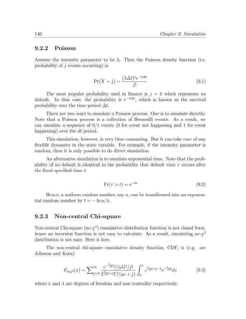
140 Chapter 9: Simulation
9.2.2 Poisson
Assume the intensity parameter to be λ. Then the Poisson density function (i.e.probability of j events occurring) is:
Pr(X = j) =(λ∆t)je−λ∆t
j!(9.1)
The most popular probability used in finance is j = 0 which represents nodefault. In that case, the probability is e−λ∆t, which is known as the survivalprobability over the time period ∆t.
There are two ways to simulate a Poisson process. One is to simulate directly.Note that a Poisson process is a collection of Bernoulli events. As a result, wecan simulate a sequence of 0/1 events (0 for event not happening and 1 for eventhappening) over the dt period.
This simulation, however, is very time consuming. But it can take care of anyflexible dynamics in the state variable. For example, if the intensity parameter israndom, then it is only possible to do direct simulation.
An alternative simulation is to simulate exponential time. Note that the prob-ability of no default is identical to the probability that default time τ occurs afterthe fixed specified time t.
Pr(τ > t) = e−λt (9.2)
Hence, a uniform random number, say u, can be transformed into an exponen-tial random number by t = − lnu/λ.
9.2.3 Non-central Chi-square
Non-central Chi-square (nc-χ2) cumulative distribution function is not closed form,hence an inversion function is not easy to calculate. As a result, simulating nc-χ2
distribution is not easy. Here is how.
The non-central chi-square cumulative density function, CDF, is (e.g. seeJohnson and Kotz):
Fncχ2(x) =∑∞
j=0
e−1/2λ(1/2λ)j/j!
21/2ν+jΓ(1/2ν + j)
∫ x
0
z1/2ν+j−1e−
1/2zdz (9.3)
where ν and λ are degrees of freedom and non centrality respectively.

Random Numbers 141
Note that a chi-square density is:
fχ2(z; k) =1
21/2kΓ(1/2k)
z1/2k−1e−
1/2zdz (9.4)
where k is the degrees of freedom. Also note that the Poisson density is:
fP (x;h) =∑∞
j=0
e−hhx
x!(9.5)
where h is the intensity parameter. Hence, we can write the CDF of the non-central,chi-square distribution as:
Fncχ2(x) =∑∞
j=0fP (j; 1/2λ)
∫ x
0
fχ2(z; ν + 2j)dz (9.6)
This implies that the CDF of a non-central, chi-square distribution is a CDFof Poisson weighted chi square distribution. Hence, to simulate the non-central,chi-square random variable, we follow the following steps:
• simulate Poisson random variable, x, with an intensity of 1/2λ
• simulate chi-square random variable, y, with the degrees of freedom as 2x +4αµ/σ2
• To simulate the short rate in the CIR model, r(t + ∆t), we first set λ =2cr(t)e−α∆t where c = 2α/σ2
(1− e−α∆t
). Then we note that in the CIR
model, the short term interest rate does not follow non-central, chi-square dis-tribution but a scaled non-central, chi-square distribution. The scaled amountis r(t+ ∆t) = y/(2c).
While the above algorithm always works, a simpler algorithm can be employedif the degrees of freedom is greater than 1. When ν > 1, the following recursive resultholds (see Johnson and Kotz):
Zncχ2(x; ν, λ) = (ZN +√λ)2 + Zχ2(x; ν − 1) (9.7)
where Zncχ2(x; ν, λ, ZN , and Zχ2(x; ν− 1) represent the random variables from non-central, chi-square, normal, and chi square respectively. In this case, we can simulatethe non-central, chi-square variable as follows:
• simulate standard normal

142 Chapter 9: Simulation
• simulate chi square with ν − 1
• degrees of freedom
• add them together.
9.2.4 Multi-variate Gaussian
To simulate multiple correlated random variables, it is important to understandCholesky decomposition. Cholesky decomposition makes it possible that we firstsimulate independent random variables and then correlate them. As a result, simu-lating many correlated random variables is extremely straightforward.
Given the correlation matrix, R, we perform the Cholesky decomposition asfollows:
CC′ = R (9.8)
where C is the Cholesky matrix. In other words, the Cholesky matrix decomposesthe correlation matrix. This is Cholesky decomposition. Let X (a vector) follow thediffusion:
dX = Mdt+ ΣCdW (9.9)
where M is the drift and Σ is a diagnal matrix of standard deviations. Then,
Ω = (dX)(dX′)
= (ΣCdW )(ΣCdW )′
= ΣCC′Σ′
= ΣRΣ′
(9.10)
To simulate the joint Gaussian distribution, it is straightforward:

Random Numbers 143
dX1
dX2
...
dXn
=
µ1
µ2
...
µn
dt+
σ1
σ2
. . .
σn
×
x1,1 · · · x1,n
0 x2,2 x2,n...
. . ....
0 0 0 xn−2,n−2 xn−2,n−1 xn−2,n
0 0 0 0 xn−1,n−1 xn−1,n
0 0 0 0 0 1
dW1
dW2
...
dWn−2
dWn−1
dWn
(9.11)
where
xj,n = ρj,n for all j 6 n (note that ρn,n = 1)
xi,j =ρi,j −
∑nk=j+1 xi,kxjk
xj,jfor i < j
xj,j =
√1−
∑n−j
k=1x2j,j+k for j < n
Take a 4-variable example and expand it as:
dX1
dX2
dX3
dX4
=
µ1
µ2
µ3
µ4
dt+
σ1
σ2
σ3
σ4
×
√
1− x212 − x2
13 − x214
ρ12−ρ14ρ24−x13x23√1−x223−x224
ρ13−ρ14ρ34√1−ρ234
ρ14
0√
1− x223 − x2
24ρ23−ρ24ρ34√
1−ρ234ρ24
0 0√
1− ρ234 ρ34
0 0 0 1
dW1
dW2
dW3
dW4
(9.12)
The model may not be Gaussian. It could be a different statistical distribution.

144 Chapter 9: Simulation
9.3 Examples
9.3.1 Black-Scholes
The most straightforward example to practice Monte Carlo is the Black-Scholesmodel, which we shall demonstrate here. The Black-Scholes model employs thefollowing log normal process for the stock price:
dS = rSdt+ σSdW (9.13)
One way to simulate the stock price is to simulate the following stochasticEuler equation:
∆S = rS∆t+ σS√
∆tε (9.14)
where ε ∼ N(0, 1). This equation can be written as:
St+∆t − St = rSt∆t+ σSt√
∆tε (9.15)
or
St+∆t = St(1 + r∆t) + σSt√
∆tε (9.16)
where ∆t is the small time step (e.g. 1/252 for one daily simulations). Note thatsubscripts here are time indexes. After a number of steps as the option reachesmaturity (e.g. 3 months, or 0.25 year), we can compute the option price as:
maxST −K, 0
for call and
maxK − ST , 0
for put. The option value today is:
C0 = e−rT Et[maxST −K, 0
= e−rT∑N
j=1
1
NmaxST,j −K, 0
(9.17)

Examples 145
The following table is an Excel exercise of 8 weekly Monte Carlo simulationresult. The basic information of this example is as follows:
Inputsinitial stock price (S0) 100∆t (week) 1/52risk-free rate (r) 0.04volatility (σ) 0.3strike (K) 98
The simulations of 1 path are done in Excel and shown below:
Outputs 1week rand num stock price
0 100.00001 -0.76519 96.89352 -0.70608 94.12183 1.41599 99.73884 -0.39640 98.17075 -0.42778 96.49916 -0.24764 95.57927 -0.58516 93.32598 -0.20290 92.6099
On this path, at the end of the 8th week, the stock price is $92.61 which is outof the money for the call option. Simulate a different path as follows:
Outputs 2week rand num stock price
0 100.00001 1.59777 106.72412 0.24837 107.90893 1.45871 114.54054 1.47683 121.66605 -1.20669 115.65186 0.26589 117.02007 -0.44651 114.93638 0.61087 117.9457
and the stock price at the end of the 8th week is $117.95 which is in the money ofthe call option, and the payoff is $17.95. Simulating a number of paths, say 1000, we
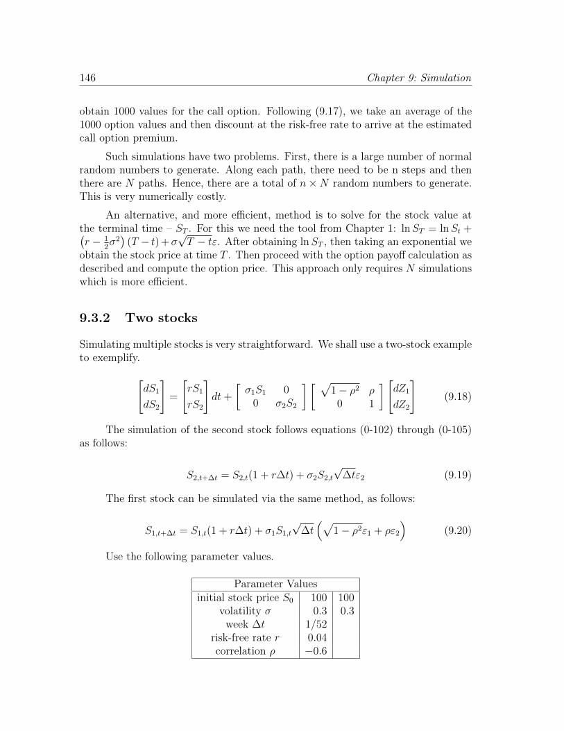
146 Chapter 9: Simulation
obtain 1000 values for the call option. Following (9.17), we take an average of the1000 option values and then discount at the risk-free rate to arrive at the estimatedcall option premium.
Such simulations have two problems. First, there is a large number of normalrandom numbers to generate. Along each path, there need to be n steps and thenthere are N paths. Hence, there are a total of n×N random numbers to generate.This is very numerically costly.
An alternative, and more efficient, method is to solve for the stock value atthe terminal time – ST . For this we need the tool from Chapter 1: lnST = lnSt +(r − 1
2σ2)
(T − t) +σ√T − tε. After obtaining lnST , then taking an exponential we
obtain the stock price at time T . Then proceed with the option payoff calculation asdescribed and compute the option price. This approach only requires N simulationswhich is more efficient.
9.3.2 Two stocks
Simulating multiple stocks is very straightforward. We shall use a two-stock exampleto exemplify.[
dS1
dS2
]=
[rS1
rS2
]dt+
[σ1S1 0
0 σ2S2
] [ √1− ρ2 ρ
0 1
][dZ1
dZ2
](9.18)
The simulation of the second stock follows equations (0-102) through (0-105)as follows:
S2,t+∆t = S2,t(1 + r∆t) + σ2S2,t
√∆tε2 (9.19)
The first stock can be simulated via the same method, as follows:
S1,t+∆t = S1,t(1 + r∆t) + σ1S1,t
√∆t(√
1− ρ2ε1 + ρε2
)(9.20)
Use the following parameter values.
Parameter Valuesinitial stock price S0 100 100
volatility σ 0.3 0.3week ∆t 1/52
risk-free rate r 0.04correlation ρ −0.6

Examples 147
We simulate 8 weeks of correlated stock prices as follows.
Outputsweek rand num norm r.n. stock price rand num norm r.n. stock price
0 100 1001 0.722067 0.588993 102.5273 0.698352 0.519665 100.33632 0.061049 -1.54603 96.01172 0.632405 0.33823 105.4153 0.435153 -0.16327 95.43343 0.771024 0.742223 108.52984 0.357303 -0.36568 94.055 0.853696 1.052417 113.40535 0.082638 -1.38754 88.698 0.288043 -0.55911 115.31016 0.742822 0.652071 91.17241 0.800278 0.842615 116.75567 0.823997 0.930706 94.77272 0.470177 -0.07482 113.84238 0.157892 -1.00316 90.89039 0.688519 0.491657 118.6433
9.3.3 Stock with random interest rates
We continue to use the Euler approximation for the stock (Black-Scholes):
dS = rSdt+ σSSdWS
St+∆t = St + rSt∆t+ σSt√
∆tεS,t+∆t
= St
(1 + r∆t+ σ
√∆tεS,t+∆t
) (9.21)
where ∆t = 1252
= 0.003968254.
But now the interest rates are random and we assume to follow the Vasicekmodel:
dr = α(µ− r)dt+ σrdWr
rt+∆t = rt + αµ∆t− αrt∆t+ σr√
∆tεr,t+∆t
= rt(1− α∆t) + αµ∆t+ σr√
∆tεr,t+∆t
(9.22)
where the two random processes are correlated with the correlation coefficient ρ :dWSdWr = ρdt.
Let (known as the Cholesky decomposition)[dWS
dWr
]=
[ √1− ρ2 ρ
0 1
] [dZS
dZr
](9.23)
Then dZSdZr = 0. Then,

148 Chapter 9: Simulation
[dS
dr
]=
[rS
α(µ− r)
]dt+
[σS 00 σr
][dWS
dWr
]
=
[rS
α(µ− r)
]dt+
[σSS 0
0 σr
] [ √1− ρ2 ρ
0 1
][dZS
dZr
] (9.24)
Hence,
St+∆t = St + rSt∆t+ σSSt√
∆tεS,t+∆t
= St
(1 + r∆t+
√∆tσS
(√1− ρ2εS,t+∆t + ρεr,t+∆t
)) (9.25)
and
rt+∆t = rt(1− α∆t) + αµ∆t+ σr√
∆tεr,t+∆t (9.26)
Use the following parameter values.
Parameter Valuesinitial value (S0/r0) 100 0.02volatility (σS/σr) 0.3 0.1
week ∆t 1/52correlation ρ −0.6
We simulate 8 weeks of correlated stock price and interest rates as follows.
Outputsweek rand num norm r.n. int. rate rand num norm r.n. stock price
0 0.02 1001 0.26516 -0.62751 0.01168 0.63801 0.35315 99.982572 0.35716 -0.36607 0.00715 0.14230 -1.07005 98.307913 0.85302 1.04946 0.02234 0.73532 0.62898 101.119234 0.68315 0.47651 0.02928 0.76893 0.73533 102.791985 0.38716 -0.28673 0.02551 0.88485 1.19960 107.228256 0.50613 0.01535 0.02600 0.34620 -0.39560 108.936297 0.87028 1.12771 0.04191 0.25562 -0.65691 100.229728 0.22975 -0.73966 0.03162 0.63994 0.35831 99.56878

Homework 149
9.4 Homework
1. VaR of one stock: Choose a stock and do the same analysis.
2. VaR of one stock and one option: Do the same analysis with the company ofyour choice.
9.5 Appendix
Theoretically, the var-cov matrix for the factors should be a diagonal matrix asfactors are orthogonal. However, in reality, we do not obtain orthogonal factorsfrom data using PCA. As a result, the following matrix is observed:

150 Chapter 9: Simulation
ΩF
=
σ11···
σ1n1
. ..
σn1n1
00
0
0
σn1+
1,n
1+
1···
σn1+
1,n
1+n2
. ..
σn1+n2,n
1+n2
00
0. .
.0
00
0
σn1+···
+nn−1,1···
σn1+···
+nn−1,nn
. ..
σn1+···
+nn,n
1+···
+nn
(9.2
7)
wher
en
1+···+
nn
=K
and
ΩF
isaK×K
mat
rix.
The
abov
em
atri
xim
plies
that
inte
r-in
dust
ryco
rrel
atio
ns
are
assu
med
0.N
ote
that
the
stan
dar
ddev
iati
ons
her
ear
efo
rth
ech
ange
sin
pri
cean
dnot
for
retu
rn.
Chapter 10
Volatility and Extreme ValueTheorem
10.1 Introduction
As we have learned so far, volatility is the key to risk management. The entire marketrisk (i.e. VaR) is based upon volatility. An inaccurate estimate of the volatility, asa result, can lead to very wrong risk management decisions. Hence, estimating theright levels of volatility is a very important job. In our analyses before, mostly thevolatility used is based upon historical estimates, which are not good reflections offuture levels of volatility. Consequently, volatility forecast is a key and importanttask.
The easiest way to obtain an estimate a future volatility is the implied volatilityfrom the options markets. As option prices are bets on future payoffs, their impliedvolatility estimates reflect what investors’ beliefs of future volatility. Unfortunately,we only have a very limited number of options contracts traded in the market place(limited tenors and most tenors are very short term, less than a year). Therefore,methods of forecasting volatility are adopted in risk management.
Another important risk management concept is to recognize the fact that rareevents are not rare. In other words, large losses are more than likely than whatpeople think. To over come this problem, probability distributions with fat tailsare proposed to replace the popular normal distribution. t distribution, Cauchydistribution, and so on are being proposed. Or alternatively, we can adopt theextreme value theory (EVT) to “fatten” the tails of a normal distribution.

152 Chapter 10: Volatility and Extreme Value Theorem
10.2 Implied Volatility and Risk-Neutral Density
The easiest and best forecast of future volatility is the implied volatility from optionand/or futures prices.1
With enough options and futures contracts we not only can estimate volatilityof any future date, we can also imply out the entire distribution of the underlyingasset. Options and futures can provide a “volatility surface” which can then be usedto imply out the risk-neutral distribution of the underlying asset.
Take the Black-Scholes model as an example. The call option formula is:
C = SN(d1)− e−r(T−t)KN(d2)
where
d1 =lnS − lnK + (r + 1/2σ2)(T − t)
σ√T − t
d2 = d1 − σ√T − t
Taking partial derivative of the call price with respect to the strike price (i.e.∂C/∂K), we arrive at:
N(d2)
which is the probability of in the money, or Pr[S > K] for a given maturity. Takinganother partial derivative with respect to the strike, we arrive at the probabilitydensity function of the underlying asset:
p.d.f. =∂N(d2)
∂K
In the Black-Scholes case, this is just a normal density. Yet this method canbe used with real options and the resulting p.d.f. is not necessarily normal. Tosummarize, the risk-neutral density of the stock can be computed as:
p.d.f =∂2C
∂K2
1Note that forwards and swaps are model-free, they do not embed volatility information (or anyother parameter). Futures and options are model dependent and hence can be used to estimatethe volatility which is one of the model parameters.

GARCH 153
Sometimes we do not have enough option contracts to derive a granular enoughdensity function and industry often uses smoothing techniques to generate “fake”option prices. The smoothing techniques vary from bank to bank.
10.3 GARCH
GARCH, or Generalized Auto Regressive and Conditional Heteroskedesticity, is amethodology to model time series of volatility. A GARCH(p, q) model specifies theevolution of the volatility as:
σ2t = ω +
∑p
i=1αiε
2t−i +
∑q
j=1βjσ
2t−j (10.1)
The estimation of GARCH is left to another chapter.
10.4 EWMA
EWMA (exponentially weight moving average) methodology for calculating thevolatility estimates.
σ2j,t = (1− λ)r2
j,t−1 + λσ2j,t−1 (10.2)
where λ is the decay factor (which is usually set between 0.99 and 0.97) and j rep-resents a tenor of choice (e.g. 3-month). EWMA is a special case of a GARCH(1,1)model as follows:
σ2t = α0 + α1σ
2t−1 + β1ε
2t−1 (10.3)
where α0 = 0, and α1 = 1− β1.
When the β’s are large and the α’s small, the volatility evolves more quickly asmore weight is placed on the most recent change in the underlying random variable,and less on the previous volatility levels. On the other hand, when the βs aresmall and the αs large, the volatility evolves more slowing resulting in a low level ofvolatility-of-volatility.
RiskMetricsTM estimated 2 the decay (λ) parameter for various regions and
2Technical Document. Document date unclear. Morgan Guaranty Trust Company Risk Man-agement Advisory Jacques Longerstaey (1-212) 648-4936 [email protected] Reuters LtdInternational Marketing Martin Spencer (44-171) 542-3260 [email protected]

154 Chapter 10: Volatility and Extreme Value Theorem
instruments as follows (their page 99, Table 5.8: Optimal decay factors based onvolatility forecasts):
Decay Parameter EstimatesCountry Fore Ex 5y Swap 10y Zero Eq Index 1y MMAustria 0.945Australia 0.980 0.955 0.975 0.975 0.970Belgium 0.945 0.935 0.935 0.965 0.850Canada 0.960 0.965 0.960 0.990Switzerland 0.955 0.835 0.970 0.980Germany 0.955 0.940 0.960 0.980 0.970Denmark 0.950 0.905 0.920 0.985 0.850Spain 0.920 0.925 0.935 0.980 0.945France 0.955 0.945 0.945 0.985Finland 0.995 0.960Great Britain 0.960 0.950 0.960 0.975 0.990Hong Kong 0.980Ireland 0.990 0.925Italy 0.940 0.960 0.935 0.970 0.990Japan 0.965 0.965 0.950 0.955 0.985Netherlands 0.960 0.945 0.950 0.975 0.970Norway 0.975New Zealand 0.975 0.980Portugal 0.940 0.895Sweden 0.985 0.980 0.885Singapore 0.950 0.935United States 0.970 0.980 0.980 0.965ECU 0.950
To estimate the parameter, one must use GARCH(1,1) with restrictions. Weleave all the econometric discussions to another chapter.
10.5 Extreme Value Theory (EVT)
The material in this section is taken from the master thesis of Krenar Avdulaj (2010)at the Charles University in Prague (p.15-19).
The Extreme Value Theory (EVT) is designed to model very large tails. Thisis know as black swans or rare events. The basic black swan or rare event story is

Extreme Value Theory (EVT) 155
that black swans or rare events are really rare. In other words, tail probabilities(probabilities for very large losses) are not as small as people think.
There are fatter tail distributions, such as t or Cauchy. Yet, a popular methodis to use EVT to model the tail probabilities. EVT is based upon the generalizedPareto distribution (cumulative density function) as given below:
Gξ,β,u(x) =
1−(
1 + ξβ(x− u)
)−1/ξ
ξ 6= 0
1− exp−x−u
β
ξ = 0
(10.4)
where u can be regarded as a high threshold, β > 0, x ≥ 0 and x ≤ −β/ξ. Further-more, x can be specified as:
x− u ≥ 0 ξ ≥ 00 ≤ x− u ≤ −β/ξ ξ < 0
The conditional distribution of excess losses over a high threshold u is definedto be:
Fu(y) = Pr[X 6 y + u|X > u] (10.5)
for 0 ≤ y ≤ v − u and v is the end point of the distribution which could be ∞ inmany cases. Then this conditional distribution of excess losses can be written interms of underlying distribution function F as:
Fu(y) =F (y + u)− F (u)
1− F (u)(10.6)
From the above expression, it seems that depending on the function shape ofF (u), the excess losses distribution can have infinite ways of asymptotic behaviors.But according to a key result in EVT, we have the following Theorem. For alarge class of underlying distributions we can find a function F (u) such that (D. V.Gnedenko 1943):
limu→v
sup06y6v−u
|Fu(y)−Gξ,β,u(x)| = 0 (10.7)
where generalized Pareto distribution Gξ,β,u(x) is a two parameter distribution func-tion as described in equation (10.4).

156 Chapter 10: Volatility and Extreme Value Theorem
10.5.1 Estimating Tails of Distributions
Using equations (10.4), (10.6), and (10.7), we can rewrite distribution function as:
F (x) = (1− F (u))Gξ,β,u(x− u) + F (u) (10.8)
To estimate the EVT tail probability Gξ,β(u)(x − u), we first need to have aproxy for F (u). For this purpose we take the obvious empirical estimator N−Nu/Nwhere N is the total number of simulation points and Nu is the number of pointslocated in the tail.3
Hence, we get the tail probability as (adjusted for the EVT):
1− F (x) =Nu
N
(1 + ξ
x− uβ
)−1/ξ
(10.9)
Note that when ξ = 0 (this is when the distribution is degenerated to Gaus-sian), the tail probability is precisely the sample statistic, which is Nu/N . If ξ 6= 0,then the tail probability is higher than Nu/N , basically adding an additional quan-tity to the tail.
A remark on the left tail estimation
The estimation of tail probability equation apparently gives the right tail. Whatwe need is the left tail estimation. To do that, we simply flip the tail from left toright. Note that losses are all negative, and hence by flipping them we satisfy x > 0.Consequently, equation (10.9) applies.
10.5.2 Estimating VaR
For a given probability α > F (x) the VaR estimate is calculated by inverting thetail estimation formula to get
∧V aR = u+
β
ξ
((N
Nu
(1− α)
)−ξ− 1
)(10.10)
Note that u = F−1(α), i.e. inverse function of F . The rationale behind theVaR equation is quite intuitive. If we adopt normal distribution for our parametric
3This is because, of course, the tail probability has a sampling statistic of Nu/N .

Extreme Value Theory (EVT) 157
VaR then the tail probability F (u) will be too small and u will be too small. As aresult, due to the reality of fat tails, we must add value to u. The amount to add isthe second term in equation (10.10). For this term to be positive, given both ξ andβ are positive, it must be that:
(N
Nu
(1− α)
)−ξ> 1
which means that:
N
Nu
<1
1− αor α < 1− Nu
N
This means that the tail probability of a real distribution must be greater(fatter) than the tail probability of a normal distribution. Otherwise, the tails areTHINNER rather than fatter. Now it is clear that the necessary condition for afatter tail using EVT is that the sampling of a real distribution must be fatterthan normal. Then the generalized Pareto distribution helps use its parameters toproperly estimate the accurate VaR.4
10.5.3 Estimating ES
Expected shortfall is related to VaR by
ESα = V aRα + E[X − V aRα|X > V aRα]
It can verified that
FV aRα(y) = Gξ,β+ξ(V aRα−u)(y)
By noting the mean of the above distribution is
(β + ξ(V aRα − u))/(1− ξ)
4For example, supposed there there are a total of 100 observations and α is 95%. Then a fattail suggest that Nu (the tail) should be more than 5 observations.

158 Chapter 10: Volatility and Extreme Value Theorem

Chapter 11
Model Risk
11.1 Introduction
Model risk has become one of the major risk management areas post-Lehman crisis.This is because too many positions (especially illiquid ones) have been marked tomodels that were either manipulated or incorrect. One obvious example is the lackof (il)liquidity discounts.
According to Wikipedia, sources of model risk are (https://en.wikipedia.org/wiki/Model-risk):
• Sources of model risk
• Uncertainty on volatility
• Time inconsistency
• Correlation uncertainty
• Complexity
• Illiquidity and model risk
famous cases in model risk are:
• Natwest – Interest rate options and swaptionsincorrect model specification.
• Bank of Tokyo-Mitsubishi – Interest rate options and swaptions.
• LTCM – lack of stress testing – Crouhy, Galai, and Mark (and over-estimatingmarket appetites – When Genius Failed by Roger Lowenstein)
160 Chapter 11: Model Risk
• Barclays de Zoete Wedd (BZW) – Mispriced currency options.
• National Australia Bank $3 Billion AUD loss on Homeside interest rate model.
• 2007-2012 global financial crisis – Over-reliance on David X. Li’s Gaussiancopula model misprices the risk of collateralized debt obligations.
quantitative approaches to model risk
• Model averaging vs worst-case approach
• Quantifying model risk exposure
• Position limits and valuation reserves
mitigating model risk
• Theoretical basis
• Implementation
• Testing
examples of model risk mitigation
• Parsimony
• Model risk premium
http://www.bostonfed.org/economic/neer/neer1997/neer697b.pdf
In March of 1997, NatWest Markets, an investment banking subsidiary of Na-tional Westminster Bank, announced a loss of £90 million due to mispriced sterlinginterest rate options. Shortly thereafter, BZW, an investment banking subsidiaryof Barclays, sustained a £15 million loss on mispriced currency options and Bankof Tokyo-Mitsubishi announced a loss of $83 million. In April of 1997, DeutscheMorgan Grenfell lost an undisclosed amount. Model errors have been blamed for allthese losses.

Part III
Credit Risk


Chapter 12
Introduction
12.1 Sources of Credit Risk
Simply speaking, credit risk is default risk. However, credit risk can be transferredin different ways. That is, there are different transactable instruments that cantransfer different parts of credit risk. Typically, there are three types of credit risk:
• bankruptcy
• migration
• spread
Bankruptcy is the ultimate default. The firm no longer operates and liquidatesits assets to pay off its debts. Debt holders lose some of their investment value(known as loss given default or severity) and stock holders lose all of their investmentvalue. Credit risk of this sort needs to evaluate the likelihood of bankruptcy (knownas probability of default, or PD) and loss given default (LGD).
Usually bankruptcies do not happen suddenly. Companies lose money andultimately lead to bankruptcy. Rating agencies monitor such transition and pro-vide their assessment of the fundamental financial healthiness of the firm via creditratings. Hence, rating migrations (especially from high to low) indicate how poorlythe firm is operating. As a result, when a firm is downgraded by rating agencies,its bond and stock prices are lowered. Empirical evidence has shown that ratingchanges have significant impacts on stock and bond prices.
Last but not least is the spread credit risk. Ratings reflect firms’ financialhealth. Yet, rating changes do not occur often. Furthermore, ratings are discrete

164 Chapter 12: Introduction
measures. Stocks and bonds are traded continuously in the marketplace. As a result,we can transfer credit risk much more quickly by trading spreads.
In this chapter, we only discuss the basic math of credit risk modeling. Thatis, we only evaluate the bankruptcy credit risk. There are models for just migrationand spread risks but are not covered here. Readers should be aware that manymigration and spread models are ad-hoc and do not relate back to default. Readersshould keep in mind that all three types of credit risk result from default becausewithout default risk, there are no migration or spread changes.
12.2 Types of Credit
The credit risk is usually modeled by the Jarrow-Turnbull model published in 1995by the Journal of Finance.
12.2.1 Corporates
Corporations borrow to finance their investment projects. There is a wide varietyof forms of how corporate borrowing ranging from short term borrowings like linesof credit, commercial papers (90 days and 180 days typically), and bank term loans(which themselves take various forms), to medium term corporate notes and bonds,to long term corporate bonds (some can be as long as 100 years!)
There is a wide variety of forms within corporate bonds fixed rate bonds,floating rate bonds (floaters), bonds with sinking funds, bonds with amortizingprincipals, convertible bonds, callable and puttable bonds, etc. Corporate bondsalso vary in terms of covenants, collaterals, and seniorities.
Rating agencies rate corporate bonds by their default likelihoods and recoveryvalues once defaults happen. Hence, ratings provide investors a rough idea of howrisky corporate bonds are in a general way. In other words, ratings summarize allthe information with a single letter to help investors understand the credit risk ofcorporate bonds. While ratings are very helpful, due to their simplicity, they areoften criticized to be inaccurate and behind market timing.
Despite many rating agencies that provide different rating systems, in generalwe have 9 rating groups:
• AAA
• AA

Types of Credit 165
• A
• BBB
• BB
• B
• CCC
• CC
• C
• D
where within each rating there could be multiple, usually three, sub-groups (callednotches).
Due to different business characteristics (business risk), we often classify com-panies into industry sectors. The highest level of classification is to divide companiesinto two groups: financial and industrial. Financial companies have high leverage ra-tios due the nature of the business, hence cannot be compared with other industrialfirms. Industrial companies are further divided into many groups. Different servicecompanies classify industrial companies differently. For example, Compustat, thelargest financial data source, classifies the companies as follows:
• Division 0: Agriculture, Forestry, And Fishing
• Division 1: Mining, and Construction
• Division 2,3: Manufacturing
• Division 4: Transportation, Communications, Electric, Gas, And SanitaryServices
• Division 5: Wholesale Trade, Retail Trade
• Division 6: Finance, Insurance, and Real Estate
• Division 7,8: Services
• Division 9: Public Administration
Combining every industry sector and every credit rating, we are able assigneach and every firm into a “cohort”. For example, 9 credit ratings (from AAA to C)and 9 industry sectors result in 81 cohorts. Within each cohort, companies shouldbe rather homogenous since they belong the same industry and rating. As a result,we can compute 81 cohort yield curves.
166 Chapter 12: Introduction
12.2.2 Sovereigns ($ denominated)
There are two major types of sovereign bonds traded in the United States (anddenominated in dollars):
• Yankee bonds
• Brady bonds
[www.investopedia.com]A Yankee bond is a bond denominated in U.S. dollarsand is publicly issued in the United States by foreign banks and corporations. Ac-cording to the Securities Act of 1933, these bonds must first be registered with theSecurities and Exchange Commission (SEC) before they can be sold. Yankee bondsare often issued in tranches and each offering can be as large as $1 billion.
Due to the high level of stringent regulations and standards that must beadhered to, it may take up to 14 weeks (or 3.5 months) for a Yankee bond tobe offered to the public. Part of the process involves having debt-rating agenciesevaluate the creditworthiness of the Yankee bond’s underlying issuer.
Foreign issuers tend to prefer issuing Yankee bonds during times when the U.S.interest rates are low, because this enables the foreign issuer to pay out less moneyin interest payments.
[wiki]Brady bonds are dollar-denominated bonds, issued mostly by Latin Amer-ican countries in the 1980s, named after U.S. Treasury Secretary Nicholas Brady.
Brady bonds were created in March 1989 in order to convert bonds issued bymostly Latin American countries into a variety or “menu” of new bonds after manyof those countries defaulted on their debt in the 1980’s. At that time, the market forsovereign debt was small and illiquid, and the standardization of emerging-marketdebt facilitated risk-spreading and trading. In exchange for commercial bank loans,the countries issued new bonds for the principal and, in some cases, unpaid interest.Because they were tradable and came with some guarantees, in some cases they weremore valuable to the creditors than the original bonds.
The key innovation behind the introduction of Brady Bonds was to allow thecommercial banks to exchange their claims on developing countries into tradableinstruments, allowing them to get the debt off their balance sheets. This reducedthe concentration risk to these banks.
The plan included two rounds. In the first round, creditors bargained withdebtors over the terms of these new claims. Loosely interpreted, the options con-tained different mixes of “exit” and “new money” options. The exit options weredesigned for creditors who wanted to reduce their exposure to a debtor country.

Types of Credit 167
These options allowed creditors to reduce their exposure to debtor nations, albeitat a discount. The new money options reflected the belief that those creditors whochose not to exit would experience a capital gain from the transaction, since thenominal outstanding debt obligation of the debtor would be reduced, and with itthe probability of future default. These options allowed creditors to retain theirexposure, but required additional credit extension designed to “tax” the expectedcapital gains. The principal of many instruments was collateralized, as were “rollinginterest guarantees”, which guaranteed payment for fixed short periods. The firstround negotiations thus involved the determination of the effective magnitude ofdiscount on the exit options together with the amount of new lending called forunder the new money options.
In the second round, creditors converted their existing claims into their choiceamong the “menu” of options agreed upon in the first round. The penalties forcreditors failing to comply with the terms of the deal were never made explicit.Nevertheless, compliance was not an important problem under the Brady Plan.Banks wishing to cease their foreign lending activities tended to choose the exitoption under the auspices of the deal.
By offering a “menu” of options, the Brady Plan permitted credit restructur-ings to be tailored to the heterogeneous preferences of creditors. The terms achievedunder these deals indicate that debtors used the menu approach to reduce the cost ofdebt reduction. Furthermore, it reduced the holdout problem where certain share-holders have an incentive to not participate in the restructuring in hopes of gettinga better deal.
The principal amount is usually but not always collateralized by speciallyissued U.S. Treasury 30-year zero-coupon bonds purchased by the debtor countryusing a combination of International Monetary Fund, World Bank, and the country’sown foreign currency reserves. Interest payments on Brady bonds, in some cases,are guaranteed by securities of at least double-A-rated credit quality held with theFederal Reserve Bank of New York.
Countries that participated in the initial round of Brady bond issuance wereArgentina, Brazil, Bulgaria, Costa Rica, Dominican Republic, Ecuador, Mexico,Morocco, Nigeria, Philippines, Poland, Uruguay.
12.2.3 Munis
¡wiki¿In the United States, a municipal bond (or muni) is a bond issued by a state,city or other local government, or their agencies. Potential issuers of municipal bondsinclude cities, counties, redevelopment agencies, school districts, publicly ownedairports and seaports, and any other governmental entity (or group of governments)

168 Chapter 12: Introduction
below the state level. Municipal bonds may be general obligations of the issueror secured by specified revenues. Interest income received by holders of municipalbonds is often exempt from the federal income tax and from the income tax of thestate in which they are issued, although municipal bonds issued for certain purposesmay not be tax exempt.
Muni bonds are as risky as corporate bonds. Rating agencies rate muni bondsas they rate corporate bonds.
12.2.4 Commercial Mortgages
Commercial mortgages have very low LTVs (loan-to-value ratios) and hence sufferfrom high default risk. Examples of commercial mortgages are:
• shopping centers
• casinos
• hotels
• rental apartments
• etc.
12.2.5 Retail Credit
The above credit risks are roughly categorized as corporate credits. That is, thecredit risk of an entity. In addition, there are also credit risks from individuals.Individuals borrow money just like corporations do and they can default on theirloans as well. This is known as retail credit risk. Due to a number of variousreasons, we must model retail credit risk different from corporate credit risk. Thereare a number retail loans that are transacted in the secondary market. We have thefollowing types of retail credit:
• Credit card
• Auto
• Student
• Home equity

Types of Credit 169
Mortgages The most important one of all is residential home mortgages. Homeowners borrow from banks to purchase their homes and use their homes as collaterals.These loans are called mortgages. Many mortgage banks lend home owners withthe deposits they receive from their depositors. Many others sell their mortgages tothe secondary market as mortgage-backed securities.
Regardless if a mortgage is lent directly by deposits or selling to the secondarymarket, the interest rate charged (called mortgage rate) on the borrower is a functionof the borrowers credit history, which is categorized as follows:
• prime
• Alt-A
• sub-prime
These mortgage rates reflect the credit quality of the borrowers and hence varywidely. Prime borrowers are the safest. They must meet many strict criteria suchas low LTV (loan to value ratio, typically less than 80%) and low PI (payment toincome ratio, usually less than 1/3). Alt-A borrowers are less safe. They may notbe high credit-risky but are classified as such due to lack of long credit history orlack of documentation. Sub-prime borrowers are regarded as unsafe or high risk,but they do not necessarily have bad credit history. Some may not have steady jobor regular income.
Credit cards Credit card loans are the money owed by card owners by notpaying the full amount each month. It is notoriously well known that credit cardinterest rates are extremely high (like 18% on a per annum basis). Credit cardloans, along with other retail lendings are packaged in “asset backed securities”and transacted in the secondary market. A credit card loan can be short or longdepending on the borrower’s consumption and financing habit. It can range from afew days to several months.
Auto loans Loans borrowed to purchase automobiles are packaged in assetbacked securities as well. However, unlike credit card loans, these auto loans arecollateralized (by the vehicles). As a result, they are much less risky than creditcard loans. In fact, the asset backed securities backed by auto loans are considerextremely safe and they often receive AAA ratings.
Student loans Student loans are government subsidized loans which are inmany cases guaranteed by the government. The student loans that are securitizedin the secondary market are performed by SLM Corporation (commonly known asSallie Mae; originally the Student Loan Marketing Association).

170 Chapter 12: Introduction
12.3 Economic Default and Liquidity Default
Economic defaults are those follow the structural models (e.g. Merton) where firmslose money over time and deplete the equity (so called “bleed to death”). Liquiditydefaults are those where firms are profitable on the accrued basis but are short ofcash to pay the immediate expenses (such as a large sum of debts due).1 This isa sudden death situation which is close to the reduced-form models. We shall seemore details in Chapter 17.
12.4 Liquidation Process
A liquidation process is a process of selling a firm’s assets under bankruptcy. Lawyersand accountants are involved in determining which debt holder should get what.This is a complex process and will take many years to finish in that all debt contractsmust be reviewed including all covenants and clauses of the debt contracts. Sellingassets can also itself be a lengthy process and many interested parties (usuallycompetitors) will pick and choose and negotiate prices.
12.5 Recovery (or Severity) and Loss Given De-
fault (LGD)
This is one of the two major building blocks of credit risk. The amount of recovery(or oppositely loss given default) severely and directly impact the credit risk. In anextreme case where recovery is 100%, the credit risk is 0 no matter how high theprobability of default (another building block) is. Recovery or LGD is also a majorplayer in portfolio risk analysis (i.e. portfolio loss function which is the foundationof all credit risk metrics.)
12.6 Probability of Default (PD)
This is another building block of credit risk. In many situations PD is more im-portant than LGD, especially when curve construction (because a preferable creditcurve is 0 recovery). There are two major approaches in constructing the credit
1This happened for Excite@Home where a convertible bond issue was due. The firm wasprofitable but short of cash. See the Appendix of Chapter 2 for details.

Probability of Default (PD) 171
curve – reduced-form approach and structural approach, to be discussed in detailsin Chapters 13 and 14.

172 Chapter 12: Introduction

Chapter 13
Reduced-Form Models
13.1 Introduction
There are two general approaches in modeling default – the structural approach andthe reduced-from approach. The reduced-form models for default, like any otherreduced-form models, take market information as given. Analogously, the structuralmodels, like many others, are built on economic fundamentals.
While details vary, the basic principle of the reduced-form models is that de-faults occur according to a Poisson process. In other words, a default event is aPoisson jump event. The representative reduced-form models for default are theJarrow-Turnbull and Duffie-Singleton models. When a Poisson jump event hap-pens, a firm is in default. Once a firm is in default, it is assumed that it will notbecome live again. As a result, a default here represent complete bankruptcy. Assetsof the company must be liquidated. The usual notion of default such as Chapter 11(bankruptcy protection) is not a default event by these models.
13.2 Survival Probability
We compute survival probabilities when we model default. The survival probabilitybetween now and some future time T for defaults is:
Q(t, T ) = e−λ(T−t) (13.1)
where λ is the “intensity” parameter of the Poisson process. This intensity parameterintuitively represents the likelihood of default. When the recovery is 0, then this

174 Chapter 13: Reduced-Form Models
value is almost identical (exactly identical in continuous time) to the “forward”probability of default.
As we can see, there is extreme similarity between the result of survival prob-ability and risk-free discount, which is P (t, T ) = e−r(T−t). In fact, we shall showthat they can be combined linearly if the recovery of a risky bond is 0. Due to thissimilarity, we shall proceed without proof (which is difficult in many situations) toborrow what we have known for the risk-free rate and use it for the intensity. In theinsurance literature, the intensity parameter is called the hazard rate.
If the intensity parameter (hazard rate) is non-constant, then we can expressthe survival probability as:
Q(t, T ) = exp
(−∫ T
t
λudu
)(13.2)
Furthermore, if the hazard rate is random, then we simply compute the riskneutral expectation:
Q(t, T ) = Et[exp
(−∫ T
t
λudu
)](13.3)
Finally, if the interest rate is random, then we must use the forward measure:
Q(t, T ) = E(T )t
[exp
(−∫ T
t
λudu
)](13.4)
Equation 13.2 represent the survival probability till a certain future time (T ).As a result, we can have a whole “curve” of survival probabilities, known as thesurvival probability curve.
Taking the derivative with respect to an arbitrary future time T of equation13.2, we get:
λT = −d lnQ(t, T )
dT(13.5)
Again, we remind the readers of the similarity between default probabilitiesand forward rates in the risk-free world.1
1The risk-free forward rate is ft,T = −d lnP (t, T )/dT .
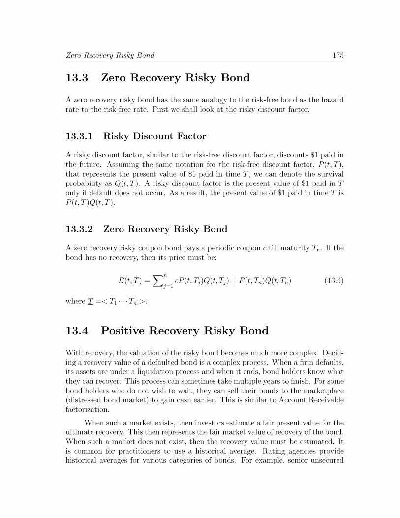
Zero Recovery Risky Bond 175
13.3 Zero Recovery Risky Bond
A zero recovery risky bond has the same analogy to the risk-free bond as the hazardrate to the risk-free rate. First we shall look at the risky discount factor.
13.3.1 Risky Discount Factor
A risky discount factor, similar to the risk-free discount factor, discounts $1 paid inthe future. Assuming the same notation for the risk-free discount factor, P (t, T ),that represents the present value of $1 paid in time T , we can denote the survivalprobability as Q(t, T ). A risky discount factor is the present value of $1 paid in Tonly if default does not occur. As a result, the present value of $1 paid in time T isP (t, T )Q(t, T ).
13.3.2 Zero Recovery Risky Bond
A zero recovery risky coupon bond pays a periodic coupon c till maturity Tn. If thebond has no recovery, then its price must be:
B(t, T ) =∑n
j=1cP (t, Tj)Q(t, Tj) + P (t, Tn)Q(t, Tn) (13.6)
where T =< T1 · · ·Tn >.
13.4 Positive Recovery Risky Bond
With recovery, the valuation of the risky bond becomes much more complex. Decid-ing a recovery value of a defaulted bond is a complex process. When a firm defaults,its assets are under a liquidation process and when it ends, bond holders know whatthey can recover. This process can sometimes take multiple years to finish. For somebond holders who do not wish to wait, they can sell their bonds to the marketplace(distressed bond market) to gain cash earlier. This is similar to Account Receivablefactorization.
When such a market exists, then investors estimate a fair present value for theultimate recovery. This then represents the fair market value of recovery of the bond.When such a market does not exist, then the recovery value must be estimated. Itis common for practitioners to use a historical average. Rating agencies providehistorical averages for various categories of bonds. For example, senior unsecured

176 Chapter 13: Reduced-Form Models
bonds recover on average 35% to 45% and junior unsecured bonds recover on average15% to 25%.
In the literature, there are two major approaches to model positive recovery.Jarrow and Turnbull (1995) assume recovery to be a fixed percentage of the facevalue of the bond and Duffie and Singleton (1997) assume the recovery to be a fixedpercentage of the market value of the bond immediately prior to default. As we shallshow later, the Jarrow-Turnbull model is particularly useful in building the creditcurve (i.e. bootstrapping) and the Duffie-Singleton model is useful in integratingwith the term structure models.
13.4.1 Recovery of Face Value – The Jarrow-Turnbull Model
When the recovery rate is a fixed amount, we can modify the pricing formula of(13.6) as follows:
B(t, T ) =∑n
j=1cP (t, Tj)Q(t, Tj) + P (t, Tn)Q(t, Tn)
+R∑n
j=1P (t, Tj)[Q(t, Tj−1)−Q(t, Tj)]
(13.7)
where c is coupon (or cash flow), P (t, T ) is risk-free discount factor between nowand time T , Q(t, T ) is survival probability between now and time T , and R is therecovery rate that is assumed constant. The last term is added due to recovery.Note that Q(t, Tj−1)−Q(t, Tj) is the default probability between Tj−1 and Tj. Notethat in continuous time, this is −dQ(t, T ) which is equal to π(t, T )dT . As a result,the above formula can be written in continuous time as:
B(t, T ) =∑n
j=1cP (t, Tj)Q(t, Tj) + P (t, Tn)Q(t, Tn)
+R
∫ Tn
t
P (t, u)[−dQ(t, u)](13.8)
The above equation is not a closed-form solution as it requires integrationover the default probability measure. One particularly easy way to keep the closed-form solution is to assume the recovery to be received at a fixed time (and notupon default). Then the above equation can be simplified assuming the recovery isreceived at Tn:
B(t, T ) =∑n
j=1cP (t, Tj)Q(t, Tj) + P (t, Tn)Q(t, Tn) +RP (t, Tn)[1−Q(t, Tn)]
(13.9)

Positive Recovery Risky Bond 177
The last term 1 − Q(t, Tn) is the cumulative default probability. This is theJarrow-Turnbull model.
We shall demonstrate numerically how the Jarrow-Turnbull model is used inpractice, which is known as “bootstrapping” or “curve cooking”. The model hasbecome the industry standard in retrieving survival probability information frommarket quotes (such as credit default swaps, or CDS). To do that the model needsto be slightly adjusted. We shall discuss this in a separate section later.
13.4.2 Recovery of Market Value – The Duffie-SingletonModel
Another easy way to arrive at a closed-form solution is to let the recovery be pro-portional to the otherwise undefaulted value. That is, upon default (at default timeu), the recovery value is Rt = δZ(t, T ) where Z(t, T ) is the price of a zero couponrisky bond as if it has not defaulted.
Under the Poisson process, for a very small time interval ∆t, we can write thebond equation as:
Z(t, T ) =Z(t+ ∆t, T )δλ∆t+ Z(t+ ∆t, T )(1− λ∆t)
1 + r∆t(13.10)
which then can be simplified to, assuming n periods between now t and maturity T :
Z(t, T ) =Z(t+ ∆t, T )(1− λ∆t(1− δ))
1 + r∆t
= Z(T, T )
[1− λ∆t(1− δ)
1 + r∆t
]n∼ Z(T, T )
[e−λ∆t(1−δ)
er∆t
]n∼ Z(T, T )e−(r+s)(T−t)
(13.11)
where s = λ(1 − δ) can be viewed as a spread over the risk-free rate. This is theDuffie-Singleton model. Z(T, T ) is the terminal value of the bond which is usuallythe face value.
A nice feature of the Duffie-Singleton model is that a coupon bond can then aportfolio of such zeros, as each coupon is treated as a zero bond it recovers marketvalue. That is:

178 Chapter 13: Reduced-Form Models
B(t, T ) =∑n
j=1cZ(t, Tj) + Z(t, Tn) (13.12)
This model is practically appealing in that it reflects the usual industry practicethat credit risk is reflected in spreads. This model is also convenient to be combinedwith existing term structure models. It simply adds a second state variable.
The drawback of the model is that the recovery parameter and the intensityparameter always are inseparable. This adds to difficulty in calibration this modelto the market.
Both the Jarrow-Turnbull and the Duffie-Singleton models assume defaults tobe unexpected like Poisson events. Different from the Jarrow-Turnbull model thatassumes fixed amount recovery (or known as recovery of face value), the Duffie-Singleton model assumes the recovery to be proportional to the market value of thedebt (known as recovery of market value) immediately prior to default.
The Jarrow-Turnbull model is suitable for bootstrapping and the Duffie-Singletonmodel is convenient to combine with term structure models. Following the similaranalysis for equations (13.2) ∼ (13.4), we can write (13.11) as:
Z(t, T ) = Et[exp
(−∫ T
t
(r(u) + s(u))du
)](13.13)
which allows us to directly model spread as another state variable. Note that s(t) =λ(t)(1 − δ) according to (13.11) and hence the spread process is similar to theintensity process. If the intensity and the risk-free rate are independent, then theDuffie-Singleton model of (13.12) is similar to (13.6) but with positive recovery.
We can easily conduct a CIR model with the Duffie-Singleton approach. Wecan have the following joint square-root process:
dr(t) = αr(µr − r(t))dt+ σr√r(t)dWr(t)
ds(t) = αs(µs − s(t))dt+ σs√s(t)dWs(t)
(13.14)
where dWr(t)dWs(t) = 0. Then (13.13) has a closed-form solution as each expecta-tion in the following equation is a CIR solution.
Z(t, T ) = Et[exp
(−∫ T
t
r(u)du
)]Et[exp
(−∫ T
t
s(u)du
)](13.15)
The following example is to demonstrate how the Duffie-Singleton model canbe easily combined with any interest rate model. In the following a simple binomial

Positive Recovery Risky Bond 179
model for the risk-free rate is given. The probabilities of the up and down branchesare 1
2and 1
2.
r=5% r+s=7.58%
$84.79
$100
$91.22
Annual Default Probability h=4% R=60%
r=7% r+s=9.63%
r=6% r+s=8.61%
$100
$100
$92.95
Figure 13.1: Duffie-Singleton Model
From the input information provided, we can compute the bond prices in thediagram, as follows:
91.215 =1
1.07[(1− 4%)× 100 + 4%× 40]
92.95 =1
1.05[(1− 4%)× 100 + 4%× 40]
84.79 =1
1.06
[(1− 4%)× 91.215 + 92.95
2+ 4%× 91.215 + 92.95
2× 0.4
]The spreads of these bonds are computed as follows:
100
91.215− 1− 7% = 9.63%− 7% = 2.63%
100
92.95− 1− 5% = 7.58%− 5% = 2.58%
92.0825
84.79− 1− 6% = 8.61%− 6% = 2.61%
where 92.0825 = 12(91.215 + 92.95). Note that these spreads are not (even though
close to) the continuous spread in the Duffie-Singleton model, which is computed as

180 Chapter 13: Reduced-Form Models
follows:1
Default Prob× Recovery + Survival Prob− 1
=1
4%× 0.4 + 96%− 1
= 2.46%
13.5 Credit Default Swap
A Credit Default Swap, or CDS, is a bilateral contract which allows an investor tobuy protection against the risk of default of a specified reference credit. The fee maybe paid up front, but more often is paid in a ”swapped” form as a regular, accruingcashflow. A CDS is a negotiated contract and there are a number of importantfeatures that need to be agreed between the counterparties and clearly defined inthe contract documentation.
First and foremost is the definition of the credit event itself. This is obviouslyclosely linked to the choice of the reference credit and will include such events asbankruptcy, insolvency, receivership, restructuring of debt and a material changein the credit spread. This last materiality clause ensures that the triggering eventhas indeed affected the price of the reference asset. It is generally defined in spreadterms since a fall in the price of the reference asset could also be due to an increasein the level of interest rates.
Many CDS contracts define the triggering of a credit event using a referenceasset. However, in many cases the importance of the reference asset is secondaryas the credit event may also be defined with respect to a class of debt issued bya reference entity. In this case the importance of the reference asset arises solelyfrom its use in the determination of the recovery price used to calculate the paymentfollowing the credit event.
The contract must specify what happens if the credit event occurs. Typically,the protection buyer will usually agree to do one of the following:
• Deliver the defaulted security to the protection seller in return for Par in cash.Note that the contract usually specifies a basket of securities which are rankedpari passu which may be delivered in place of the reference asset. In effect theprotection seller is long a “cheapest to deliver” option.
• Receive Par minus the default price of the reference asset settled in cash. Theprice of the defaulted asset is typically determined via a dealer poll conducted

Credit Default Swap 181
within a few weeks to months of the credit event, the purpose of the delaybeing to let the recovery price stabilize.
Some CDS have a different payoff from the standard Par minus recovery price.The main alternative is to have a fixed pre-determined amount which is paid outimmediately after the credit event. This is known as a binary default swap. In othercases, where the reference asset is trading at a significant premium or discount toPar, the payoff may be tailored to be the difference between the initial price of thereference asset and the recovery price.
The protection buyer automatically stops paying the premium once the creditevent has occurred, and this property has to be factored into the cost of the swappayments. It has the benefit of enabling both parties to close out their positionssoon after the credit event and so eliminates the ongoing administrative costs whichwould otherwise occur.
A CDS can be viewed as a form of insurance with one important advantage –efficiency. Provided the credit event in the default swap documentation is definedclearly, the payment due from the triggering of the credit event will be made quickly.Contrast this with the potentially long and drawn out process of investigation andnegotiation which may occur with more traditional insurance.
However it is possible to get a very good idea of the price of the CDS using asimple “static replication” argument. This involves recognizing that buying a CDSon a risky par floating rate asset which only defaults on coupon dates is exactlyequivalent to going long a default-free floating rate note and short a risky floatingrate note of the same credit quality. If no default occurs, the holder of the positionmakes a net payment equal to the asset swap spread of the asset on each coupondate until maturity. This spread represents the credit quality of the risky floater atissuance. If default does occur, and we assume that it can only occur on couponpayment dates, the position can be closed out by buying back the defaulted asset inreturn for the recovery rate and selling the par floater. The net value of the positionis equal to the payoff from the default swap. The following table summarizes.
CDS vs. FloaterEvent Riskless FRN Risky FRN CDSAt inception Pay par Pay par 0No default Receive LIBOR Receive LIBOR + spread Pay spreadUpon default Receive par Receive recovery + par − recoveryMaturity Receive par Receive par 0
From the above table, it is clear that the spread of a CDS must equal to thespread of the equivalent risky FRN to avoid arbitrage.

182 Chapter 13: Reduced-Form Models
13.6 Restructuring Definitions by ISDA
CDS contracts provide default protection. When a default occurs, CDS buyersstop paying the premium (spread), deliver the defaulted bond (cheapest if possible),and collect full face value as payment. However, default is hard to define. It isextremely rare for a company to file bankruptcy. What is usually happening isthat losses happen over the years and reduce the asset value of the company, toa point where the company is at the brink of bankruptcy. Then the managementof the company will start looking for alternatives to save the firm. One popularalternative to save the firm is to ask debt holders to change their debt contracts tothe company known as debt restructuring. Debt restructuring often means thatdebt holders convert parts of their debts into equity and participate in the operationof the firm. To protect their own interests, debt holders, especially large ones, willbe willing to agree to debt restructuring.
Hence debt restructuring is commonly regarded as a form of default. However,each restructuring can be very different. Some restructurings are major and equiva-lent to defaults. But some could be minor as precautionary actions to avoid furtherdeterioration of the firm, which are not equivalent to default.
To regulate if a CDS is triggered, ISDA (International Swaps and DerivativesAssociation) defines various restructuring standards:
• Full restructuring (FR), based on the ISDA 1999 Definition
• Modified restructuring (MR), based on the ISDA 2001 Supplement Definition
• Modified-modified restructuring (MMR), based on the ISDA 2003 Definition,
• No restructuring (NR).
• The definitions are as follows:
FR Any bond of maturity up to 30 years
MR T 6 T < T + 30 months
MMR Allow additional 30 months for the restructured bond.
For other obligations, same as MR.
CDS contracts traded in different regions follow different ISDA conventions.

Why Has the CDS Market Developed So Rapidly? 183
13.7 Why Has the CDS Market Developed So
Rapidly?
CDS is the most popular credit derivatives contract and has grown rapidly in late90’s and early 00’s. The following is a direct quote of Rene Stulz’s article on CDS(2010):2
Back in the mid-1990s, one of the first credit default swaps provided pro-tection on Exxon by the European Bank for Reconstruction and Development toJP Morgan (Tett, 2009). It took months to negotiate. By 1998, the total size ofthe credit default swap market was a relatively small $180 billion (Acharya, En-gle, Figlewski, Lynch, and Subrahmanyam, 2009). The credit default swap mar-ket has grown enormously since then, although there is no definite measure of howmuch. Based on survey data from the Bank for International Settlements (BIS) athttp://www.bis.org/statistics/derstats.htm, the total notional amount of the creditdefault swap market was $6 trillion in 2004, $57 trillion by June 2008, and $41trillion by the end of 2008. Credit-default swap contracts that insure default riskof a single firm are called single-name contracts; in contrast, contracts that provideprotection against the default of many firms are called multi-name contracts. 3
In addition to the efficiency in hedging and transferring credit risk, the poten-tial benefits of CDS include:
• A short positioning vehicle that does not require an initial cash outlay
• Access to maturity exposures not available in the cash market
• Access to credit risk not available in the cash market due to a limited supplyof the underlying bonds
• The ability to effectively exit credit positions in periods of low liquidity
• Off-balance sheet instruments which offer flexibility in terms of leverage
• To provide important anonymity when shorting an underlying credit
2“Credit Default Swaps and the Credit Crisis,” Journal of Economic Perspectives, Volume 24,Number 1, Winter 2010, pp. 73-92.
3Stulz noted that DTCC statics are a lot smaller.

184 Chapter 13: Reduced-Form Models
13.8 Relationship between Default Probabilities
and CDS Spreads – Use of the Jarrow-Turnbull
Model
There is a simple formula (using the Jarrow-Turnbull model) that relates the CDSspread, the risk-free rate, default/survival probabilities, and the fixed recovery rate.Due to the swap nature, CDS, similar to IRS (interest rate swap), has two legs –floating and fixed. The floating leg of a CDS contract is called the protection leg asit pays only if default occurs. The fixed leg of a CDS contract is called the premiumleg because the fixed payments (i.e. spreads) are like insurance premiums. As ina standard swap contract, at inception, the values of the two legs must equal eachother. This is how CDS spreads are calculated. Recently affected by the crisis, CDSpremiums have been split into an upfront and a spread (which is the index, suchas CDX, trading convention). As we shall see later, this extra calculation does notadd any complexity to the model. We simply deduct the upfront amount from theprotection value of the CDS. For now, we shall proceed with no upfront.
Using the formulation given earlier, the protection and premium values of aCDS are as follows:
Vprot(t, T ) = (1−R)∑n
i=1P (t, Ti)[Q(t, Ti−1)−Q(t, Ti)]
Vprem(t, T ) = s(t, T )∑n
i=1P (t, Ti)Q(t, Ti)
(13.16)
where Tn = T . As a result, the spread (known as par spread) can be computed as:
s(t, T ) =(1−R)
∑ni=1 P (t, Ti)[Q(t, Ti−1)−Q(t, Ti)]∑n
i=1 P (t, Ti)Q(t, Ti)(13.17)
Note that (13.17) (for CDS) and (13.7) (for bond) are very similar. Thenumerator of (13.17) is similar to the recovery value in (the second line of ) (13.7)and the denominator is similar to the (first line of (13.7) coupon value. This shouldnot be surprising as CDS is a natural hedge to the bond. In other words, buy a bondand a CDS is equivalent to buying a default-free bond. If we add the protectionvalue in (13.16) to the coupon bond value in (13.7), recovery disappears and thebond as a result becomes default-free.
Note that (13.17) assumes no accrued interest if default occurs in betweencoupons. In reality there are accrued interests on both legs and they may not beequal. If default is assumed to happen on cashflow days only, then there is noaccrued interest. Note that if there is an upfront, we simply deduct it from the

Back-of-the-envelope Formula 185
protection value, Vprot.
13.9 Back-of-the-envelope Formula
In a one-period model where default is a Bernulli event, as the following picturedemonstrates,
p
1 p− pay spread (s)
if survive
receive 1 - R
if default
Figure 13.2: One-period Default Diagram
We know that for the CDS to have 0 value it must be true that:
p(1−R) = (1− p)s (13.18)
Note that risk-free discount cancel from both sides. Hence, we arrive at thefamous back-of-the-envelope formula for the default probability (by ignoring theterm p× s which is small):
p =s
1−R(13.19)
This formula, while simple, provides a powerful intuition of spreads and defaultprobabilities. If the recovery is 0, then spread is (forward) default probability. Thisis not only true in (13.19) but also true in continuous time. Spreads are not equal to(i.e. smaller) forward default probabilities in that they are compensated by recovery.Note that CDS buyers acquire default protection by paying spreads as an insurancepremium. If recovery is high, the protection value is low, and so should be thespread. In an extreme case where the recovery is 100%, the spread should be 0,which is suggested by (13.19).

186 Chapter 13: Reduced-Form Models
13.10 Bootstrapping (Curve Cooking)
We need credit curves to price credit derivatives. Credit curves are obtained fromliquid cash products such as CDS or corporate bonds. Due to the liquidity concern,CDS is a better choice for curve cooking.
The basic bootstrapping idea of constructing a risky curve is the same as therisk-free curve. We use a pricing formula to back out the parameter(s). In thetraditional fixed income world (Treasuries and IRS), we back out spot and forwardrates from the market prices of bonds and swap rates. Here, we back out survivalprobabilities from a series of CDS contracts. As in the world of traditional fixedincome, we need a term structure of CDS spreads in order to back out the entiresurvival probability curve. A popular smoothing technique in LIBOR curves ispiece-wise flat.
The CDS market has been standardized over the years to have the followingon-the-run maturities: 1, 2, 3, 5, 7, and 10 years to maturities. As in the IRSmarket, these contracts are on-the-run which are issued periodically. In the earlyyears, only 5-year CDS contracts were issued. A few years ago, the market started totrade 10-year CDS contracts. The other maturities have gradually been introducedto the market but their liquidity is still a concern. Assume for now that we observemarket prices of these CDS spreads.
13.11 Poisson Assumption
From (13.2) ∼ (13.4), we know that if we assume piece-wise flat intensity values,then the survival probability can be approximated as follows:
Q(t, Tn) = exp−∑n
i=1λi(Ti − Ti−1)
(13.20)
where t = T0.
13.12 Simple Demonstration (annual frequency)
To make matters simple, we assume CDS spreads are paid annually. There are 6CDS spreads observed in the market (1, 2, 3, 5, 7, 10). Take Disney as an example.On 12/23/2005, we observe the following spreads (in basis points):

Simple Demonstration (annual frequency) 187
CDS quotesterm sprd
1 92 133 205 337 4710 61
Continue to assume fixed 0.4 recovery ratio under MR for Disney. The follow-ing binomial chart presents possible cash flows. Lets assume 5% risk-free rate.
1p
1 11Q p= − spread = 0.0009
if survive
1 - recovery rate = 0.6
if default
Figure 13.3: First period
CDS is a swap contract so there is no cash changed hands on day 1. Hence,it must be the case that the expected payment (9 basis points) equals the expectedcompensation (60%). In a single period, since both payment and compensation arediscounted, the risk-free does not matter. Note that the survival probability for oneyear is Q1 = 1− p1 (which is also equal to e−λ1 if we assume the Poisson process fordefaults). Hence, using 5% interest rate, we have:
0.6× (1−Q1)− 0.0009×Q1
1.05= 0
which is solved as:0.6× (1−Q1) = 0.0009×Q1
and Q1 = 0.9985. λ1 can be solved for as − lnQ1 to be 0.001499, or 14.99 basispoints. Hence, the survival and default probabilities are 99.85% and 0.15% respec-tively.
Now we proceed to bootstrap the second period.

188 Chapter 13: Reduced-Form Models
spread =
0.0013
10.0015p =
2p
21 p−
10.9985Q =
spread =
0.0013
1 - recovery =
0.6 1 - recovery =
0.6
2Q
Figure 13.4: Two-period Default Diagram
There are three scenarios. Either Disney defaults in period 1, or default inperiod 2, or survive in period 2 (note that to survive till period 2, Disney must firstsurvive period 1). We know the first default probability, which is p1 = 0.0015. Butwe do not know the other two probabilities. Using the same Poisson algorithm, wecan compute the second year present value as:
0.6× p2 − 0.0013× (1− p2)
1.05
Note that this quantity itself is not 0; but combining it with the first year cashflows is:
0.6× 0.0015 + 0.9985(−0.0013 + 0.6×p2−0.0013×(1−p2)
1.05
)1.05
= 0
Solve for p2 to get 28.62 basis points. Under the Poisson assumption, e−λ2 =1 − p2 and as a result, λ2 = − ln(1 − p2) = 0.002865 or 28.65 basis points. Theconditional survival probability is 1 − p2 = 99.7138%. The unconditional survivalprobability, Q2, equals (1−p1)(1−p2) which is 99.5645%. The unconditional defaultprobability is 1− 99.5645% = 0.4355%.
Similar process applies to all periods as the following figure depicts. Due tothe limitation of the space in the table, Q(t, v) is replaced with Q(τ) where τ = v−t.
The results are given as follows. The first three columns are taken from the

Simple Demonstration (annual frequency) 189
1 - recovery
1 - recovery
3p
4p
spread
1p
2p
spread
spread
spread
1 - recovery
1 - recovery
11 p−
21 p−
31 p−
41 p−
1Q
2Q
Figure 13.5: Multi-period Default Diagram
market. Columns A and B are the same spread input given earlier. Column C isthe risk-free discount factors that are computed using 5% flat in the example.
CDS BootstrappingA B C D E FTerm Market Risk-free Fwd. Surv.Pr. Def.Pr.τ Spread P (τ) λ(τ) Q(τ) −dQ(τ)1 0.0009 0.9512 0.0015 0.9985 0.00152 0.0013 0.9048 0.0029 0.9956 0.00293 0.0020 0.8607 0.0059 0.9898 0.00584 0.8187 0.0092 0.9808 0.00915 0.0033 0.7788 0.0092 0.9718 0.00906 0.7408 0.0150 0.9573 0.01447 0.0047 0.7047 0.0150 0.9431 0.01428 0.6703 0.0176 0.9267 0.01649 0.6376 0.0176 0.9106 0.016110 0.0061 0.6065 0.0176 0.8948 0.0158

190 Chapter 13: Reduced-Form Models
CDS Bootstrapping (cont’ed)G H I J K L
P (τ)× Prem. Prot. Model Cond.P (τ)Q(τ) [−dQ(τ)] Leg Leg Spread Def.Pr.0.9498 0.0014 0.9498 0.0009 0.0009 0.00150.9009 0.0026 1.8507 0.0024 0.0013 0.00290.8520 0.0050 2.7027 0.0054 0.0020 0.00580.8030 0.0074 3.5056 0.0099 0.0028 0.00920.7568 0.0070 4.2625 0.0141 0.0033 0.00920.7092 0.0107 4.9717 0.0205 0.0041 0.01480.6646 0.0100 5.6363 0.0265 0.0047 0.01480.6212 0.0110 6.2575 0.0331 0.0053 0.01740.5806 0.0103 6.8381 0.0393 0.0057 0.01740.5427 0.0096 7.3808 0.0450 0.0061 0.0174
Column E presents the survival probabilities that are computed sequentiallyas in equation (13.20):
Q(t, Tn) = exp−∑n
i=1λi(Ti − Ti−1)
= Q(t, Tn−1) exp −λn(Tn − Tn−1)
(13.21)
For example, Q(0, 2) = 0.9956 = 0.9985 × e−0.0029×(2−1). Column F is theunconditional default probabilities which is the differences are two consecutive sur-vival probabilities. For example, 0.0029 = 0.9985 − 0.9956. Column G is knownas the risky discount factor (introduecd earlier), or $1 present value with defaultrisk. These values are needed in order to compute the default swap spread, i.e. thedenominator of (13.17). Similarly, column H provides the values for the numeratorof (13.17). Columns I and J are accumulations of columns G and H respectively.Column K is the division of column J by column I, which is the spread of CDS.The values of this column must match the market quotes in column B. In fact, wesolve for column D so that values in column K are identical to values in column B.Finally, column L contains conditional default probabilities, each of which equals1−Q(t, Tj)/Q(t, Tj−1). We note that the conditional default probabilities are close tothe intensity values (λ), as they should, in that they are exactly equal in continuoustime.
The table presented here provides a nice algorithm for further automate thecalculations for more complex situations in reality, which we shall demonstrate later.Once all the λj values are bootstrapped out, we can then compute any survivalprobability of any future time, as follows:

In Reality (quarterly frequency) 191
Q(t, v) = Q(t, Tn−1) exp −λn(v − Tn−1) (13.22)
where Tn−1 < v < Tn. For example, the survival probability of 6.25 years is 0.9769×e−0.0098×(6.5−5) = 0.9627.
13.13 In Reality (quarterly frequency)
In the above example, we assume spreads are paid annually. As a result, the calcu-lation is quite simple. In reality, this is not the case. Spreads are paid by the swapmarket convention which is quarterly. In this case, default can occur at any quarter.We then need to alter the one period calculation shown above.
Note that within a year (for the first few spreads), all per-quarter defaultprobabilities are equal. This is because we have only one spread (e.g. 0.0009 in year1) to cover four quarters. The basic formula is still the same. Mainly we solve thefollowing equation for p (note that at each period, the interest rate is 1.25%):
xi = x0 + 0.6p1 + (1− p1)xi−1
xn = x0
(13.23)
where n represents the number of periods that shares the probability. For the firstyear, n = 4 and x0 = 0.000225. We then solve for p1 = 0.000375 or 3.75 basis pointsand λ1 = 0.0015. The full expansion of this equation is shown in the Appendix.
Note that while this equation is solvable by hand if proper re-arrangement ofterms is performed, it is much faster if we set up the equation and use the Solverin Excel. This equation can be set up recursively as the discounting and expectedvalues are nested. We can set up an Excel sheet to compute all the results. As ademonstration, we provide the results up the 3 years.
The layout of the table is the same as before. The frequency of the CDSpremium payments is now quarterly (see column A). Column B is still market CDSspreads that are available every four quarters. Column C is quarterly risk-freediscount factors (at 5%). Columns E ∼ H are computed similarly to the previoussection, only with quarterly frequency.
Columns, I, J, and K are computed similarly to the previous section but onlyevery year. Note that column K is column J ÷ column I × 4 in order to annualizeto match annual CDS market quotes in column B.
Readers should complete the table for the full 10 years.

192 Chapter 13: Reduced-Form Models
CDS BootstrappingA B C D E F
Market Risk-free Fwd. Surv.Pr. Fwd.Def.Pr.Term Spread P (τ) λ(τ) Q(τ) −dQ(τ)0.25 0.9876 0.0015 0.9996 0.0003750.5 0.9753 0.0015 0.9993 0.0003750.75 0.9632 0.0015 0.9989 0.0003751 0.0009 0.9512 0.0015 0.9985 0.0003741.25 0.9394 0.002868 0.9978 0.0007161.5 0.9277 0.002868 0.9971 0.0007151.75 0.9162 0.002868 0.9964 0.0007152 0.0013 0.9048 0.002868 0.9956 0.0007142.25 0.8936 0.00586 0.9942 0.0014572.5 0.8825 0.00586 0.9927 0.0014552.75 0.8715 0.00586 0.9913 0.0014533 0.002 0.8607 0.00586 0.9898 0.001451
CDS BootstrappingG H I J K L
premium protection computed cond.P (τ)Q(t) P (τ)[−dQ(τ)] leg leg spread surv.prob.0.9872 0.00040.9746 0.0004 0.99960.9621 0.0004 0.99960.9498 0.0004 3.8737 0.0009 0.0009 0.99960.9373 0.0007 0.99930.925 0.0007 0.99930.9129 0.0007 0.99930.9009 0.0006 7.5498 0.0025 0.0013 0.99930.8884 0.0013 0.99850.8761 0.0013 0.99850.8639 0.0013 0.99850.8519 0.0012 11.0302 0.0055 0.002 0.9985

Chapter 14
Corporate Finance Approach ofModeling Default
14.1 Merton Model
This approach of modeling default is called structural approach. It does not assumedefaults as an unexpected event but rather a firm’s failure to pay its debts. Theearliest model is Black-Scholes (1973) and Merton (1974) who regard the equity ofthe firm as a call option. This is because the equity of the firm has a residual claimof the firm’s assets. In a simple example where the firm has only one zero coupondebt, the face value of the debt is the strike of the call option. When the asset valueat the maturity of the debt is above the face value, the firm is able to pay off itsdebt and the equity receives the residual value of A(T ) − K where A is the assetvalue of the firm at the maturity date, T , of the debt and K is the face value ofthe debt. Otherwise (the asset value is smaller than the face value), the equity isworthless.
Figure 14.1 describes the payoffs graphically. The vertical axis is value of theassets of the firm. The horizontal axis is time. The horizontal line represents the facevalue of the debt, which is flat over time. In the example, a one-year horizon, weeklyintervals are used. In Figure 14.1, two samples of the asset value are presented – onegood and one bad. The good sample is a profitable sample where the firm does welland the asset value increases (and is higher than the debt face value at time T ). Thebad sample is where the firm loses money and the asset value ends up lower than thedebt face value. In the good sample, the debt is paid in full and the equity receivesthe residual amount A(T )−K. In the bad sample, the firm defaults anfd the debtholder receives a recovery value of A(T ) and the equity holder receives nothing. Onthe very right of the diagram is the log normal distribution that describes the asset

194 Chapter 14: Corporate Finance Approach of Modeling Default
0
50
100
150
200
250
300
350
400
0 4 8 12 16 20 24 28 32 36 40 44 48 52
Weeks
DD
PD
T
t
T
T T
T
A K
E A K
D K
>
⇓
= − =
0
T
T
T T
A K
E
D A
<
⇓
= =
tA
Figure 14.1: Merton Model
price. The area below the default barrier is the probability of default (commonlyabbreviated as PD). As a result, the equity value and equity volatility in this simplecase can be priced by the Black-Scholes model:E(t) = A(t)N(d1)− e−r(T−t)KN(d2)
σE = σN(d1)A
E
(14.1)
where σE is the equity volatility and:
d2 = lnA(t)−lnK+(r−σ2/2)(T−t)σ√T−t
d1 = d2 + σ√T − t
r is the risk-free rate, and σ is the asset return volatility. The debt value which isthe difference between asset and equity is then equal to:
D(t, T ) = A(t)− E(t)
= A(t)[1−N(d1)]︸ ︷︷ ︸Recovery value
+ e−r(T−t)KN(d2)︸ ︷︷ ︸Survival value
(14.2)
On the right hand side of the equation, the debt value is decomposed into twoparts – surivial value and recovery value. The survival value is the amount received

Merton Model 195
by the debt holders if the firm survives. In this case it is the face value weighted bythe survival (in-the-money) probability N(d2) and discounted at the risk-free rate.The recovery value is the amount received by the debt holders if the firm defaults.In this case it is the asset value weighted by the default probability and discountedat the risk-free rate. But since the asset value is random, we must compute thefollowing expected value: e−r(T−t)Et [A(T )IA<K ] which is equal to the recovery valuegiven above.
Asset Value
Risk-free Debt
Value Risky Debt
Value
Loss Given
Default
Asset Value
Asset Value
Figure 14.2: Risky Debt
Figure 14.2 describes the equation graphically. The upper-left panel is the risk-free debt whose payoff is fixed regardless of the value of the firm. The upper-rightpanel is the payoff of the risky debt. When the firm is doing well (i.e. survival), thepayment is full (i.e. face value) but when the firm is not doing well (i.e. default), thepayment is the recovery value (i.e. asset value). The bottom panel is the differencebetween the risk-free debt and the risky debt, which gives the result of the loss givendefault. The convolution of the area and the probabilities is the expected loss (EL).
Note that D(t, T ) < e−r(T−t)K which is the risk-free debt value. The (risk-neutral) default probability is p = 1 − N(d2). The following diagram is usually

196 Chapter 14: Corporate Finance Approach of Modeling Default
used to visualize how the Black-Scholes-Merton model works. The plotted are twopossible sample paths of the asset value, one drifts upward and the other driftsdownward. The asset value starts at 100 with the default barrier at 50. One samplepath stays above the default barrier and is a survival path and one crosses the barrierand is a default path. To be explored fully later, the log difference between the assetvalue and the default barrier is known as the distance to default, or DD.
14.2 KMV Model
In 1989 Stephen Kealhofer, John McQuown and Oldrich Vasicek founded companyKMV. They commercialize the Merton (Black-Scholes) model to provide quanti-tative credit ratings of companies. They coined the term EDF (expected defaultfrequency) using DD. They use equation (14.1) to compute the distance to default(DD) which is d2, because:
d2 =E[lnA(T )]− lnK√
V[lnA(T )](14.3)
Given that A(T ) follows a log normal process, this DD makes sense. Andnaturally the probability of default (PD) is 1 − N(d2), or N(−d2). The expectedrecovery (since actual recovery A(T ) is random) is A(t)[1−N(d1)].
The Merton model allows for only one single debt. To accommodate the multi-debt problem, KMV empirically estimated the one-year equivalent debt value to be:
One Year Equivalent Debt = Short Term Debt +Long Term Debt
2
=Short Term Debt + Total Debt
2
EDF is similar to PD (i.e. 1 − N(d2), or N(−d2)) (but the translation is aKMV secret) and used to decide a rating for the company. KMV also use the modelto predict defaults. See Stein (2002).
Recently, KMV also uses barrier option models (details later) to better capturemultiple debts and complex volatility forecast methods (such as GARCH) to improvethe historical equity volatility estimates that are not very reliable.

The Geske Model 197
14.3 The Geske Model
Although the Black-Scholes-Merton model reflects the reality that the only reasonfirms default is due to failure to pay, it is a one period model which is too limitedto be used for a regular firm that has multiple debts.
Geske extended the model to include multiple debts. Take a two-period ex-ample and assume the firm issues two zero coupon bonds, expiring at T1 and T2,with face values K1 and K2 respectively. Default at T1 is defined by Geske (1984)as the firm value less than the face value of the first debt plus the market value ofthe second debt, that is V1 < K1 +D(T1, T2) where D(T1, T2) is the market value ofK2 at time T1.
The solution to the equity value and equity volatility can be derived fromGeske’s compound call option (call on call) model:1
E(t) = A(t)M(h1+, h2+; ρ)− e−r(T2−t)K2M(h1−, h2−; ρ)− e−r(T1−t)K1N(h1−)
σE = σM(h1+, h2+; ρ)A
E(14.4)
where N(·) is the uni-variate standard normal probability and M(·, ·; ρ) is the bi-variate standard normal probability, and:
ρ =
√T1 − tT2 − t
hj± =lnA(t)− ln Aj + (r ± σ2/2)(Tj − t)
σ√Tj − t
(14.5)
Note that A2 = K2 is the critical value for the assets to trigger default at T2
and A1 is the solution to K1 = E(T1), as follows:
K1 = A(T1)N(x+)− e−r(T2−T1)K2N(x−)
x± =ln A(T1)− lnK2 + (r ± σ2/2)(T2 − T1)
σ√T2 − T1
which is the critical value for default at time T1; and . Recall that E(T1) is theBlack-Scholes value (due to the fact that in the last period, the equity is just a
1Note that the equation indicates that the survival probabilities are N(h1−) and M(h1−, h2−; ρ)for one year and two years respectively.

198 Chapter 14: Corporate Finance Approach of Modeling Default
simple call option). The two debt values are a bit complex to solve, but the closed-form solutions are given as follows:
D(t, T1) = A(t)[1−N(y1+)] + e−r(T1−t)K1N(y1−)
D(t, T2) = A(t)[N(y1+)−M(h1+, h2+; ρ)]− e−r(T1−t)K1[N(y1−)−N(h1−)]
+e−r(T2−t)K2M(h1−, h2−; ρ)
(14.6)
where
yj± =lnAj−1 − lnKj + (r ± σ2/2)(Tj − Tj−1)
σ√Tj − Tj−1
It is clear that the expected recover value is A(t)[1 − M(h1+, h2+; ρ)] forthe entire firm; A0[1 − N(y1+)] for debt K1; and A(t)[N(y1+) −M(h1+, h2+; ρ)] −e−r(T1−t)K1[N(y1−)−N(h1−)] for debt K2.
Note that Geske assumes each time the firm pays off its maturing debt withnew equity. As a result, the default condition becomes:
A1 < K1 +D(T1, T2)
A1 −D(T1, T2) < K1
E(a)1 < K1
(14.7)
which is, the equity value after paying off debt K1 must be greater than K1. Inother words, the equity value after paying off debt includes the new equity thatequals K1. Hence, this value must be equal to at least K1. If not, then it indicatesthat the firm cannot issue new equity, which implies obvious default. Table 14.1demonstrates the balance sheet before and after paying off K1.
At time 1T
Before 1K is paid off After 1K is paid off (with equity)
1A or 1( )AT 1K
1,2 1( )D A
( )1bE
1A or 1( )AT
1,2 1( )D A
( ) ( )11 1
a bE E K= +
Table 14.1: Balance Sheet at Time T1

The Geske Model 199
The default barrier can be calculated A1 = K1 +D1,2(A1) as D1,2 is a functionof A1. Note that A2 = K2 as this is a two period model and the firm liquidates atT2.
Suppose a company has two zero coupon debts, one and two years to maturityand each has $100 face value. Also suppose the assets are currently worth $400and the debts are together worth $170 on present value basis. This is graphicallyrepresented by the following balance sheet:2
Balance Sheet as of year 0
assets 400 Maturity 1t = debt 90
Maturity 2t = debt 80
Equity 130
total 400 Total 400note: both debts have face values of $100
Table 14.2: Balance Sheet at Year 0
First, assume that one year later, the asset grows to $450 and the firm facesthe first debt payment of $100. The firm at this time should raise equity to pay forthe first debt so that the asset value will not have to be decreased. The asset valueafter paying off the first debt is still $450. Assume that at this time (t = 1), thesecond debt, now only a year from maturity, has a value of $90. As a result, theequity should be $360 (= $450 − $90) that includes $100 new equity and $260 oldequity. The balance sheet becomes:
Now, instead of the assets being worth $450, suppose that the firm made somebad investment decisions and the asset’s value drops to $150. A bad economy andlower asset value imposes a higher default risk on the second debt so it is pricedlower at $75 due to its higher risk. Hence, the resulting equity value of old equityand of the should be raised equity, or debt due plus net equity, drops to $75 (150− $75 = $100 − $25) . The firm, as in the previous case, would like to raise equityto pay off the first debt. But the new equity value needs to be $100 to retire thedebt due which creates a clear contradiction. This means that the new equity ownerpays $100 in cash but in return receives a portion of $75. No rational investor wouldinvest equity in this firm.
Since the firm cannot raise equity capital to continue its operation, it shouldnot be considered a going concern. There is point where the potential new equity
2We assume the risk free rate to be about 10%. Since the company is extremely solvent, bothdebts are roughly priced at the risk free rate.

200 Chapter 14: Corporate Finance Approach of Modeling Default
Balance Sheet
as of year 1 before payment of first debt
assets 450 Maturity 1t = debt 100
Maturity 2t = debt 90
Equity 260
total 450 Total 450
Balance Sheet
at year 1 after payment of first debt
assets 450 maturity 2t = debt 90
old equity 260
new equity 100
total 450 Total 450
note: issue new equity to pay for the first debt
Table 14.3: Balance Sheet at Year 1
owner is indifferent and this is the going concern breakeven point for the company.Suppose the (break-even) asset value in one year is falls to $186.01. At this assetvalue, the second debt is worth $86. Consequently, the new equity owner has $100and the old equity has $0.01. And we know that the default point is $186.3
Table 14.4 shows the relationships between the market value of debt (two-yeardebt at year 1) and market value of equity in previous examples.
We can clearly see that any asset value lower than $186 will cause default andshould require other than a going concern opinion. However, with $186 of assets, thecompany can pay the first debt due and continue to operate. One could also considerselling assets to pay off the first debt without raising any new equity. However, thisapproach to claim dilution would cause the second debt to drop significantly in valueas in Table 14.5.
The reason is that the equity immediately has an option value at the cost ofthe remaining debt. In the above hypothetical tables, we assume $10 is transferredfrom debt to equity. At t = 0, the debt holders know about this even when there isno information asymmetry. As a result, they will pay less for the debt.
Usually, the company will roll over old debt to new debt instead of issuing
3This value is precisely the “implied strike price” in the Geske model. We should notice that$186.01 ∼ $186 in this example. We leave a minor amount, $0.01, to old equity holders in orderto make this example more reasonable.

The Geske Model 201
Balance Sheet
as of year 1 before payment of first debt
assets 186.01 one-year debt 100
two-year debt 86
Equity 0.01
total 186.01 Total 186.01
Balance Sheet
as of year 1 after payment of first debt
assets 186.01 two-year debt 86
old equity 0.01
new equity 100
total 186.01 Total 186.01
note: issue new equity to pay for the first debt
Table 14.4: Balance Sheet at Year 1
Balance Sheet
as of year 1 before payment of first debt
Assets 186 one-year debt 100
two-year debt 86
Equity 0
total 186 Total 186
Balance Sheet
as of year 1 after payment of first debt
assets 86 two-year debt 76
old equity 10
total 86 Total 86
note: selling asset to pay for the first debt
Table 14.5: Balance Sheet at Year 1

202 Chapter 14: Corporate Finance Approach of Modeling Default
equity. In the case of extreme solvency, this is not a problem. But in the case ofnear default, as described above, we have Table 14.6.
Balance Sheet
as of year 1 before payment of first debt
assets 186.01 one-year debt 100
two-year debt 86
Equity 0.01
total 186.01 Total 186.01
Balance Sheet
as of year 1 after payment of first debt
assets 186.01 two-year debt 86
new debt 100
old equity 0.01
total 186.01 Total 186.01
note: issue new debt to pay for the first debt
Table 14.6: Balance Sheet at Year 1
The principal of the new debt can be extremely high to reflect the very riskysituation in order to get a $100 to retire the first issue. Because the existing debtmatures earlier (and hence has a higher seniority) its value should be the samewhether there is new equity or debt. The equity will give a different claim whethernew equity is raised or new debt is issued. With new equity the original equity willreturn a small portion after the second debt issue is repaid. With new debt, theoriginal equity will get the entire return if the asset value increases after both debtissues are repaid. In the equilibrium, the original equity value should return to 0.01.It should not matter if the funds come from new equity or new debt at just overbreak-even point. Either way, the result holds and the old equity holders have a$0.01 value.
Under the current measurement for going concern status, companies will usu-ally receive a going concern opinion at $186 and probably at $150. The companycontinues to survive and operate. Now at $150 value, the company is not able toraise capital, but it is certainly able to pay the debt with its assets and leave thesecond debt with $50. Under this condition, the junior debt will be worth less than$50, possibly very little since debt holders do not have the safe covenant to preventmanagers/shareholders from selling assets to pay the senior debt. The transferringof wealth from debt owner to equity owner is what we define as the agency problem.

The Leland-Toft Model 203
As long as the company spends assets to pay the earlier maturing debt, the latermaturing debt holders will be hurt and shareholders will benefit.
We note that at the due date of the first debt, the company faces a decisionwhether to pay the debt obligation. This is a compound option question in that ifthe company decides to pay, the company continues to survive much like exercisingthe compound option to keep the option alive. The company’s survival criterionrelies upon whether the company can raise new equity capital. In this analysis, thetechnical condition of staying solvent (paying the coupon) is that the company mustuse new equity to pay for the coupon. If such new equity conceptually cannot beraised, then the company should go bankrupt. Interestingly, this condition translatesinto another equivalent condition that the market value of the assets of the companymust stay above the market value of the liabilities at the moment of the coupon.This condition is regarded as the no-arbitrage condition and should be the breakevenpoint in value for receiving a clean going concern audit.
14.4 The Leland-Toft Model
The Leland-Toft model (which is an extension of the Leland model) is anotherstructural model that extended the Black-Scholes-Merton model to include multipledebts. Different from the Geske model, the Leland-Toft model assumes continuouscoupons and continuous issuance and redemption of the debts. As a result, the firmhas a steady-state debt level that will not change, as the amount of debt issuedexactly cancels the amount of debt redeemed.
Note that in the Leland-Toft model, we remove tax shield and dead-weight costfrom the model to make it a fair comparison to other models. The model withouttax shield and deadweight cost is given as:
D =C
r+
(K − C
r
)(1− e−rT
rT− I)
+
(H − C
r
)J (14.8)
where C is the continuous coupon, K is the face value of debt that expires in timeT and:
I =1
rT
(G− e−rTF
)J =
1
zσA√T
(−(b−a+z)N [q−]q− + b−a−zN [q+]q+
)F = N [h−] + b−2aN [h+]
G = b−a+zN [q−] + b−a−zN [q+]
(14.9)
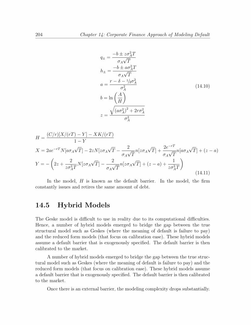
204 Chapter 14: Corporate Finance Approach of Modeling Default
q± =−b± zσ2
AT
σA√T
h± =−b± aσ2
AT
σA√T
a =r − δ − 1/2σ2
A
σ2A
b = ln
(A
H
)
z =
√(aσ2
A)2
+ 2rσ2A
σ2A
(14.10)
H =(C/r)[X/(rT )− Y ]−XK/(rT )
1− Y
X = 2ae−rTN [aσA√T ]− 2zN [zσA
√T − 2
σA√Tn[zσA
√T ] +
2e−rT
σA√Tn[aσA
√T ] + (z − a)
Y = −(
2z +2
zσ2AT
N [zσA√T ]− 2
σA√Tn[zσA
√T ] + (z − a) +
1
zσ2AT
)(14.11)
In the model, H is known as the default barrier. In the model, the firmconstantly issues and retires the same amount of debt.
14.5 Hybrid Models
The Geske model is difficult to use in reality due to its computational difficulties.Hence, a number of hybrid models emerged to bridge the gap between the truestructural model such as Geskes (where the meaning of default is failure to pay)and the reduced form models (that focus on calibration ease). These hybrid modelsassume a default barrier that is exogenously specified. The default barrier is thencalibrated to the market.
A number of hybrid models emerged to bridge the gap between the true struc-tural model such as Geskes (where the meaning of default is failure to pay) and thereduced form models (that focus on calibration ease). These hybrid models assumea default barrier that is exogenously specified. The default barrier is then calibratedto the market.
Once there is an external barrier, the modeling complexity drops substantially.

Hybrid Models 205
We can the use the First Passage Time mathematics. There are several barrier optionmodels that are popular. The first one is the flat barrier option model introducedfirst by Rubinstein and Reiner (1991).
A barrier option is an option whose payoff is activated (knocked in) and ter-minated (knocked out) when a barrier is reached by the stock price before maturity.Due the barrier can be higher or lower than the current stock price, barrier optionsare classified as down-and-in and down-and-out barrier options whose barrier liesbelow the current stock price; and up-and-in, and up-and-out barrier options whosebarrier lies above the current stock price.
Down-and-in and up-and-in barrier options become call or put options whenthe barrier is reached. Similarly, down-and-out and up-and-out barrier options be-come worthless when the barrier is reached.
The barrier option problem is the first passage time problem. Assume thestandard Black-Scholes model that the stock price follows the log normal process.Let the barrier be H and the strike be K. If the barrier is below the current stockprice, i.e. St > H, then the risk neutral probability that the stock price stays aboveboth H and K is either:
N
(lnSt − lnK + (r − 1/2σ2)(T − t)
σ√T − t
)
−(StH
)1− 2rσ2
N
(2 lnH − lnSt − lnK + (r − 1/2σ2)(T − t)
σ√T − t
)(14.12)
if H < K or
N
(lnSt − lnH + (r − 1/2σ2)(T − t)
σ√T − t
)−(StH
)1− 2rσ2
N
(lnH − lnSt + (r − 1/2σ2)(T − t)
σ√T − t
)(14.13)
if H > K. Note that the first part of equation (13-102) is just the probability ofST > K. The second part of equation (13-102) is the joint probability that ST > Kand Sτ < H. As a result, the difference is the joint probability that ST > K andSτ > H. When H > K, then staying above the barrier automatically guarantees inthe money for the option and we simply replace K by H.
As a result, the down-and-out barrier call option model (i.e. St > H) can bederived as:

206 Chapter 14: Corporate Finance Approach of Modeling Default
Cdo = e−r(T−t)Et[(ST −K)1ST>K∩Sτ>H ]
= e−r(T−t)Et[ST1ST>K∩Sτ>H ]− e−r(T−t)KEt[1ST>K∩Sτ>H ]
= StΠ+ − e−r(T−t)KΠ−
(14.14)
where
Π± = N
(lnS − lnK + (r ± 1/2σ2)(T − t)
σ√T − t
)−(S
H
)1− 2rσ2
N
(2 lnH − lnV − lnK + (r ± 1/2σ2)(T − t)
σ√T − t
)(14.15)
if H < K or
Π± = N
(lnSt − lnH + (r ± 1/2σ2)(T − t)
σ√T − t
)−(StH
)1− 2rσ2
N
(lnH − lnSt + (r ± 1/2σ2)(T − t)
σ√T − t
)(14.16)
if H > K. Note that the two results for Π− are just probability of first passagetime. The results for Π+ can be obtained via the change of measure.
The down-and-in barrier call option model can be derived by subtracting thedown-and-out option model from the Black-Scholes model: Cdi = CBS − Cdo.
If the barrier is above the current stock price, i.e. St < H, then the risk neutralprobability that the stock price stays above both H and K is either:
N
(lnSt − lnK + (r − 1/2σ2)(T − t)
σ√T − t
)
−(StH
)1− 2rσ2N
(2 lnH − lnSt − lnK + (r − 1/2σ2)(T − t)
σ√T − t
)−N
(lnSt − lnK + (r − 1/2σ2)(T − t)
σ√T − t
)(14.17)
if H < K or
N
(lnSt − lnH + (r − 1/2σ2)(T − t)
σ√T − t
)
−(StH
)1− 2rσ2N
(lnH − lnSt + (r − 1/2σ2)(T − t)
σ√T − t
)−N
(lnSt − lnH + (r − 1/2σ2)(T − t)
σ√T − t
)(14.18)

Hybrid Models 207
if H > K. Note that the first part of equation (13-105) is just the probability ofST > K. The second part of equation (13-105) is the joint probability that ST > Kand Sτ < H. As a result, the difference is the joint probability that ST > K andSτ > H. When H > K, then staying above the barrier automatically guarantees inthe money for the option and we simply replace K by H.
The second one is by Black and Cox (1976) where the barrier is not flat butexponentially decayed. The first passage time (survival probability) by Black andCox is given as follows:
N
(lnV − lnKe−γ(T−τ) + (r − a− 1/2σ2)(τ − t)√
σ2(T − t)
)−(
V
Ke−γ(T−t)
)1−2(r−a−γ)
σ2
×
N
(2 lnKe−γ(T−t) − lnV − lnKe−γ(T−τ) + (r − a− 1/2σ2)(τ − t)√
σ2(T − t)
)(14.19)
where K is the barrier amount, γ is the decay rate of the barrier (in other words,the barrier is smaller currently than close to maturity), τ is the default time (i.e.,the first passage time to the boundary), and V is the asset value. To put it plainly,if t∗ is the first passage time to the boundary, then the probability that t∗ ≥ τ isgiven by the above equation.
The last one is the CreditGrades model (2002) that was developed by GoldmanSachs, JP Morgan, Deutsche Bank, and RiskMetrics. This is essentially a randombarrier model. The technical document can be downloaded from creditgrades.com.The main equation is its approximation formula for the survival probability, asfollows:
Q(t) = N
(−A
2+
ln d
A
)− dN
(−A
2− ln d
A
)(14.20)
where
A =√σ2Sξ
2t+ λ2
d =1
1− ξeλ
2
ξ =E
E +D
and λ is the volatility parameter for the stochastic barrier, E is the equity value

208 Chapter 14: Corporate Finance Approach of Modeling Default
and D is the “target” debt value. Hence, it is logical to view ξ as the leverage ratio.With the survival probability function, we can proceed with CDS valuation.

Chapter 15
Credit Portfolio and CreditCorrelation
15.1 Introduction
So far we have been assessing single-name credit risk and how to model it. Thekey risk management factor – correlation has not been discussed. As in market riskmanagement, correlation is the key driving factor to lower the risk. Little or evennegative correlation among assets can dramatically reduce the risk of a portfolio.However, correlation in credit is much complex than it is in market risk. In marketrisk, especially in parametric VaR, correlation is used among normally distributedasset returns, and as a result a simple covariance matrix can describe very well howdiversification works and then VaR is easily inferred.
The reason why correlation in market risk so easily used is of course a resultof normally distributed asset returns. In market risk, although there are variouscriticisms on normally distributed asset returns, it is not a bad first order approxi-mation to regard asset returns as normal. Unfortunately, such an approximation istotally unsuitable in credit risk.
First of all, credit losses are only negative. That is, there is no gain in defaults– everyone suffers. Hence, symmetry in normality is out of question. Secondly, bothPD (probability of default) and LGD (loss given default) are both random and inter-related (see Introduction). These two variable add extra complexity to modeling thecredit risk, unlike in market risk there is only one variable – returns of assets.
Hence, here we first introduce the concept of credit correlation. We start withdefault correlation. We use a simple and yet powerful credit derivative contract –credit default basket to introduce the concept credit correlation. Briefly, we demon-

210 Chapter 15: Credit Portfolio and Credit Correlation
strate, via default basket, how correlation in credit risk can be misleading. Then,via the example, we show that why industry moves to copula to replace credit corre-lation. Finally, a full example of CDO (collateralized debt obligation) is introducedto utilize copula in its entirety.
15.2 Basics
The following Venn diagram helps explain the basic setup of portfolio credit riskvaluation.
A B
A&B
Figure 15.1: Venn Diagram for Default
where A and B represent the two default events for company A and company Brespectively. The area in the middle represents joint default.
In order to properly correlate default events, maintain the flexibility of freelyspecifying individual default probabilities, and be able to uniquely define a jointdistribution, we use conditional default probabilities to describe the dependencyof two default events (rather than specifying the correlation). In other words, wespecify the default probability of the second bond given that the first bond hasalready defaulted.
For a single period, the default event should follow a Bernoulli distributionwhere 0 represents no default and 1 represents default. Under the Bernoulli distri-bution, the specification of the conditional probability (given the marginal proba-bilities) uniquely defines the joint default probability. The joint default probabilitycan be formally delineated as:
p(A ∩B) =
p(A|B)p(B) orp(B|A)p(A)
(15.1)

Basics 211
where A and B represent default events, i.e. a short hand notation for A = 1 and B= 1.
This specification of the joint distribution is desirable in that it is realistic indefining the default relationship between two bonds. If two bonds have differentdefault probabilities (marginals) but they are extremely highly correlated, it means(in our model) that if the less risky one defaults, the riskier one will surely defaultbut not the other way around. Imagine a small auto part supplier whose sole clientis a large automobile manufacturer. If the manufacturer defaults, it is highly likelythat the small part supplier will eventually default as well. The small part sup-plier may also default on its own, independent of what happens to the automobilemanufacturer.
For example, we let A be default on the part of the manufacturer and Bbe the default on the part of the small supplier. Each has 10% and 20% defaultprobability for the period, respectively. The part supplier is completely dependentupon the manufacturer, i.e. the conditional default probability of the supplier onthe manufacturer is one. Then the joint probability of both firms defaulting is:
p(A ∩B) = p(B|A)p(A)
= p(A)
= 10%
(15.2)
Hence, we obtain the following joint distribution for the two companies:
Bivariate Bernulli Distribution0 1 A
0 80% 0% 80%1 10% 10% 20%B 90% 10% 100%
The survival of the small supplier depends completely on the large auto man-ufacturer:
p(B|A) =p(A ∩B)
p(A)= 100% (15.3)
The dependency of the manufacturer on the supplier can be calculated to be:
p(A|B) =p(A ∩B)
p(B)=
10%
20%= 50% (15.4)

212 Chapter 15: Credit Portfolio and Credit Correlation
which is equal to the ratio of the two individual default probabilities. The uncondi-tional correlation of the two companies is 0.6667. The two companies can also haveperfectly negative dependency: default of one company implies the survival of theother. In this case, the conditional probability is:
p(BC |A) = 1
or
p(B|A) = 0
(15.5)
Using the numbers in the previous example yields the following joint distribu-tion:
Bivariate Bernulli Distribution0 1 A
0 70% 10% 80%1 20% 0% 20%B 90% 10% 100%
Notice that, even though there is perfect negative dependency, the uncondi-tional correlation is only −0.1667.
The examples here show that perfect dependency does not translate to perfectcorrelation. This is because dependency is directional but correlation is not. In thefirst case, A defaults causes B defaults but not vice versa. Hence the dependencyof B on A is 100% but A on B is only 50%. The correlation is in between, 67%. Inthe second case, A can survive only if B defaults and vice versa. This is perfectlynegative dependency but the correlation is only −17%. The unconditional defaultcorrelation is calculated as follows:
ρ(A,B)either=
p(B|A)p(A)− p(A)p(B)√p(A)(1− p(A))p(B)(1− p(B))
or=
p(A|B)p(B)− p(A)p(B)√p(A)(1− p(A))p(B)(1− p(B))
(15.6)
So it is seen that it is not possible to reach 100% or -100% correlation unlessthe following conditions are satisfied:
• p(A) = p(B) for 100% correlation
• p(A) + p(B) = 1 for -100% correlation

Default Baskets (First to default) 213
When there is perfect dependency (i.e. p(B|A) = p(A|B) = 1), for ρ(A,B) =1, it must be true that:
1 =p(A)(1− p(B))√
p(A)(1− p(A))p(B)(1− p(B))
=
√p(A)(1− p(B))√(1− p(A))p(B)
(15.7)
in which the only solution is p(A) = p(B). When there is perfect negative de-pendency (i.e. p(BC |A) = 1, or equivalently p(B|A) = 0, and vice versa), forρ(A,B) = −1, it must be true that:
−1 =−p(A)p(B)√
p(A)(1− p(A))p(B)(1− p(B))
1 =
√p(A)p(B)√
(1− p(A))(1− p(B))
(15.8)
in which the only solution is p(A) + p(B) = 1.
15.3 Default Baskets (First to default)
Default baskets usually contain only a few credit names (individual bonds). Thefirst-to-default basket pays principal and accrued interest minus the recovery valueof the first defaulted bond in the basket.
For the sake of easy exposition, we examine a two-asset basket with no coun-terparty risk. The model can easily be extended to a multi-asset basket, but thevalue must be solved numerically. Following the previous discussion, the probabilityof the first-to-default in a two-asset case is p(A ∪ B). To find the value of such aprobability, we first need to find values of CDS spreads for A and B. Given that thisis a single period model, we can use 13.19 with 40% recovery rate. Then, we havethe CDS spread for A as 20%× (1− 40%) = 12% (or 1200 basis points) and for Bas 10% × (1 − 40%) = 6% (or 600 basis points). As a result, we can compute thespread for the first-to-default (FTD) as:
p(A ∪B) = p(A) + p(B)− p(A ∩B) = 10% + 20%− 10% = 20%
s(A ∪B) = p(A ∪B)× (1− 40%) = 12%(15.9)
We can also calculate the second-to-default (STD) as follows:

214 Chapter 15: Credit Portfolio and Credit Correlation
p(A) + p(B)− p(A ∪B) = p(A ∩B) = 10%
s(A ∩B) = 6%(15.10)
It is easy to demonstrate that the basket value is a (negatively) linear functionof the default correlation. When the default correlation is small (or even negative),the issuers tend to default alternately: this increases the basket risk. When thecorrelation is large, the issuers tend to default together: this decreases the basketrisk. As will be demonstrated below, the value of the default basket will vary betweenthat of a single default swap (when there is perfect dependency) and the sum of thetwo individual default swaps (when there is zero dependency).
Note that in the event of perfect dependency, i.e. p(B|A) = 1, then p(A∩B) =p(B|A)p(A) = p(A) and then p(A ∪ B) = p(B). As a natural result, the spread forthe FTD equals the spread for B (same can be said if p(A|B) = 1), which impliesthat the value of the basket is equal to the value of a single name default swap.
On the other hand, if the dependency is perfectly negative, i.e. p(BC |A) = 1or p(B|A) = 0, then p(A ∪ B) = p(A) + p(B). Then the spread of the FTD equalsthe sum of the spread for A and the spread for B, which implies that the value ofthe basket is equal to the sum of the two individual swaps. (Note that in this casethe value of the STD is 0, as one of the two must survive.)
Note that if there is no dependency and the two companies were to have defaultprobabilities that sum to exactly 100%, then the joint distribution would degenerateand result in an unconditional correlation of −1.
The results can be extended to multiple assets, though the calculations ofthe probabilities become multi-dimensional. We can use Monte-Carlo methods tocalculate the joint normal probabilities in high dimensions. We can write down thevaluation equation as follows:
V = Et[P (t,minuj)Iminuj<T (1−Rj(uj))Nj
](15.11)
where I is the indicator function, uj is the default time of the j-th bond, Rj isrecovery rate of the j-th bond, and Nj is the notional amount of the j-th bond. Thebasket pays when it experiences the first default, i.e. minuj.
Obviously, the above equation has no easy solution when the default events (ordefault times, uj) are correlated. Hence, in the following, we only solve the modelunder indepedent defaults. Under independence, we can write (15.11) as:
V =
∫ T
t
∑n
i=1P (t, u)
[−dΠi
j=1Qj(t, u) + dΠi−1j=0Qj(t, u)
](1−Ri(u)) (15.12)

Copula and CDO Pricing 215
where Q0(t, u) = 1 and hence dQ0(t, u) = 0. The above formula assumes that thelast bond (i.e. bond n) has the highest priority in compensation, i.e. if the last bondjointly defaults with any other bond, the payoff is determined by the last bond. Thesecond to last bond has the next highest priority in a sense that if it jointly defaultswith any other bond but the last, the payoff is determined by the second to lastbond. This priority prevails recursively to the first bond in the basket.
15.4 Copula and CDO Pricing
15.4.1 Background
A Collateral Debt Obligation, or CDO, is a set of securities known as tranches thatare backed by a pool (portfolio) of default-risky fixed income securities (e.g. cor-porate bonds, loans, default swaps, and asset backed securities). These obligations,or tranches, are then sold to investors. Commonly it is set up as a SPV (specialpurpose vehicle) as depicted in Figure 15.2.
CDO
(SPV)
Cash
Issued
Securities
Senior
Tranche
Mezz.
Tranche
Equity
Tranche
Loans
Bonds
Receivables Cash
Issued
Securities
Asset Manager
Hedge Provider
Figure 15.2: CDO Structure
These SPVs are “paper companies” set up by various financial institutions(most likely investment banks) and the assets are also acquired from these financialinstitutions. During the crisis, it had become apparent that many banks dumpedtheir bad assets to these SPVs and then issued very opaque tranches so that investorswould not find out how bad the quality of the assets is in the pool.
While frauds had been committed and lawsuits had been filed (e.g. JP Morgans$13 billion settlement with the U.S. Justice Department), efforts have been madeto resume the securitization market and try to make the market more healthy andtransparent.

216 Chapter 15: Credit Portfolio and Credit Correlation
15.4.2 Basics
A CDO is a collection of bonds (or loans and in that case it is called CLO) that areresold to the secondary market in tranches. The actual tranche structure is highlyflexible and takes no definite form but in general, it has a waterfall structure wheretranches are paid off in a sequential order. This structure is known as the n-th losstranche structure. For example, a CDX CDO is a CDO with 125 credit default swapswith US$ 10 million notional. The CDO is sliced up into the following tranches:0-3%, 3-7%, 7-10%, 10-15%, and 15-30%. Losses over 30% are extremely unlikely(due to collaterals ) and hence are not analyzed. The structure is the standardwaterfall structure that the first tranche (equity tranche) takes upon loss of defaultup to 3%, or $300,000, Then the following mezzanine tranche will take over the next4% loss (from 3 to 7%), or $400,000, and so on.
As we see above, the basic structure of a CDO is similar to that of a CMO(Collateral Mortgage Obligations) in that the waterfall defines the sequence of thepayoff to each tranche. The difference lies in tranche payoffs. A typical CMO uses allits revenues (mortgage payments) to pay its senior tranche. After the senior trancheis completely paid, the mezzanine tranche can take over. A CDO structure is to payevery tranche if there is enough revenue (coupons from bonds). Any reduction inrevenue due to defaults is taken from the junior tranche, and then the mezzaninetranche, and then the senior tranche.
The primary pricing objective of pricing CDOs is to compute the spreads of thetranches. However, an equally important objective is to study the loss distributionsof the tranches. As it will be clear later, even though spreads can be computedfor the investors to trade, risk managing these tranches require much more thanjust the spreads. Due to the extremely exotic loss distributions, without the wholedistribution, it is nearly impossible to do a good job in risk management.
A typical number of a CDOs constituents is in hundreds. And all constituentsare highly correlated. As a result, to understand the loss distribution of a CDOis difficult. Monte Carlo simulation is the usual technique to accomplish such agoal. However, for 125 bonds in a CDO, there will be 125×124
2= 7750 correlations
to estimate and simulations themselves take a large amount of time. As a result, afast approximation method is developed. The use of FI quickly reduces the multi-dimensional problem to uni-dimensional. However, some simplifications must bemade. While details are to be seen later, the major intuition is as follows. First, wemust assume a factor model (single factor to begin with) through which all bondsare correlated. This limits the flexibility of how assets are correlated and yet itprovides consistency (of correlation estimates) over time and a parametric structurethat makes FI possible. Secondly, we must assume a barrier structural model thatexplain how defaults occur.
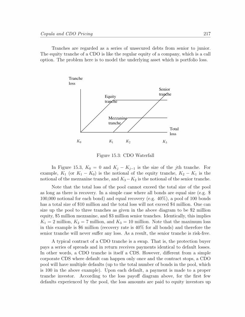
Copula and CDO Pricing 217
Tranches are regarded as a series of unsecured debts from senior to junior.The equity tranche of a CDO is like the regular equity of a company, which is a calloption. The problem here is to model the underlying asset which is portfolio loss.
Tranche
loss
Equity
tranche
Mezzanine
tranche
Senior
tranche
Total
loss
1K
2K
0K
3K
Figure 15.3: CDO Waterfall
In Figure 15.3, K0 = 0 and Kj − Kj−1 is the size of the jth tranche. Forexample, K1 (or K1 − K0) is the notional of the equity tranche, K2 − K1 is thenotional of the mezzanine tranche, and K3−K2 is the notional of the senior tranche.
Note that the total loss of the pool cannot exceed the total size of the poolas long as there is recovery. In a simple case where all bonds are equal size (e.g. $100,000 notional for each bond) and equal recovery (e.g. 40%), a pool of 100 bondshas a total size of $10 million and the total loss will not exceed $4 million. One cansize up the pool to three tranches as given in the above diagram to be $2 millionequity, $5 million mezzanine, and $3 million senior tranches. Identically, this impliesK1 = 2 million, K2 = 7 million, and K3 = 10 million. Note that the maximum lossin this example is $6 million (recovery rate is 40% for all bonds) and therefore thesenior tranche will never suffer any loss. As a result, the senior tranche is risk-free.
A typical contract of a CDO tranche is a swap. That is, the protection buyerpays a series of spreads and in return receives payments identical to default losses.In other words, a CDO tranche is itself a CDS. However, different from a simplecorporate CDS where default can happen only once and the contract stops, a CDOpool will have multiple defaults (up to the total number of bonds in the pool, whichis 100 in the above example). Upon each default, a payment is made to a propertranche investor. According to the loss payoff diagram above, for the first fewdefaults experienced by the pool, the loss amounts are paid to equity investors up

218 Chapter 15: Credit Portfolio and Credit Correlation
to K1 ($2 million in the example). Then losses of the next defaults are paid tomezzanine investors up to K2. The process continues until the either all bonds inthe pool default or the CDO contract expires, whichever earlier.
As a result, as long as we can model the total loss, we can easily compute thecumulative tranche loss and in turn the value of the protection leg and the value ofthe premium leg of each tranche. The valuation of a CDO (i.e. its tranches) is avery technical matter and hence beyond the scope of this book. Interested readerscan refer to, for example, Chen’s Mathematical Finance for full details.
15.4.3 Factor Copula
In the standard factor copula model used now as the industry standard, we writethe following:
xi =√ρWM +
√1− ρWi (15.13)
where xi is the factor that computes the default probability for firm i and ρ is thebase correlation. Both WM and Wi are normally distributed with 0 mean. Hencexi is normally distributed. For any given period (say a year), we can write theconditional default probability as follows:
pi|f = Pr (xi < Ki|WM = f) = Pr(√
ρf +√
1− ρWi < Ki
)= Pr
(Wi <
Ki−√ρf√
1−ρ
)= N
(Ki−√ρf√
1−ρ
)= N
(N−1(pi)−
√ρf√
1−ρ
)(15.14)
where Pr(xi < Ki) = N(Ki) = pi is the unconditional default probability. Naturally,∫Ω(f)
pi|fφ(f)df = pi (15.15)
where φ(f) is the standard normal distribution for the common factor, f . Con-ditional on the market factor f , firms default independently. Hence, under theconditional probability pi|f , defaults are independent. There are several methodsto model conditional loss distribution. Here we introduce the Vasicek method, theFourier inversion method, and the recursive algorithm.

Copula and CDO Pricing 219
The Vasicek method is a special case of the Fourier inversion method and therecursive algorithm. It assumes that the bond notionals and recoveries in the CDOpool are the same. The Fourier inversion method and the recursive algorithm haverelative advantages and disadvantages. Recursive algorithm is faster but it worksbest when the recoveries of the bonds are the same. Fourier inversion method is moregeneral but it is generally slower and it gives continuous loss distribution where thetrue loss distribution is discrete.
15.4.4 The Vasicek Model
If the exposures (notionals) are identical, then the percentage loss can be found bycarrying out the following equation,
Pr( L = i/m ) =
(m
i
)Pr(A1 < K1, · · · , Ai < Ki, Ai+1 > Ki+1, · · · , Am > Km)
=
(m
i
)∫ ∞−∞
Pr(A1 < K1, · · · , Ai < Ki, Ai+1 > Ki+1, · · · , Am
> Km|WM = f)dF (WM < f)(15.16)
Independence conditional on WM = f gives:
Pr(L = i/m) =
(m
i
)∫ ∞−∞
Pr(A1 < K1|WM = f) · · ·Pr(Ai < Ki|WM = f)
Pr(Ai+1 > Ki+1|WM = f) · · ·Pr(An > Kn|WM = f)dF (WM < f)
=
(m
i
)∫ ∞−∞
∏i
j=1N(N−1(pj)−
√ρf√
1−ρ
)∏m
j=i+1N(−N−1(pj)−
√ρf√
1−ρ
)dF (WM < f)
(15.17)
Note that “m choose i” or (m i)′, is only symbolic and not a real combinationfunction. Vasicek further simplifies by setting all probabilities equal, i.e. pj = p:
Pr(L = i/m) =
(m
i
)∫ ∞−∞
N(N−1(p)−√ρf√
1−ρ
)iN(−N−1(p)−√ρf√
1−ρ
)m−idF (WM < f)
(15.18)

220 Chapter 15: Credit Portfolio and Credit Correlation
Here (m i)′ is the combination function. The integral can be implementedeither via Riemman sum or Monte Carlo simulations. Cumulative loss is:
Pr(L 6 i/m) =∑i
`=0Pr(L = `/m) (15.19)
This can be very computationally expensive if probabilities are not equal, andstill quite expensive if probabilities are equal (sum over m-choose-i terms). Vasicek(Limiting Loan Loss Probability Distribution) proposes an asymptotic formula andSchonbucher presents the FFT method. The FFT method is more plausible becauseit is computationally possible and less limitation than the Vasicek method.
15.4.5 Fourier Inversion and Recursive Algorithm
To evaluate CDOs correctly, two alternative (competing) methods are commonlyused – Fourier Inversion and Recursive Algorithm. These methods can accuratelycalculate tranche values of a CDO. The Fourier Inversion method is more flexibleand the Recursive Algorithm method is faster. For the details of the these methodsand examples, see for example Chen’s Financial Mathematics.
15.4.6 An Example
In the following, we show an example where there are 100 bonds in the pool. Thisprobability is exaggerated so to magnify the behavior of the loss distribution. Therecovery rate is 40% for all bonds. Hence, the maximum loss of the pool is 60% ofthe total pool size.
The shape of the loss distribution is very sensitive to the correlation. In thefollowing several diagrams, we shall see how the loss distribution changes as thecorrelation increases. On the left is plotted the loss distribution for various correla-tion numbers when the default probability is 6%. On the right is plotted the samecorrelation scenarios when the default probability is 2%.
As we can see obviously, the lower is the default probability; the more right-skewed is the loss distribution, which implies the safer is the pool. Also we seethat distribution is multi-modal when the correlation is high. The multi-modalphenomenon is more pronounced when the default probability is high. This can beeasily seen from the two graphs when the correlation is 0.5. Figure 15.4 depicts theloss functions under various assumptions.
Once we obtain the loss distribution, we can then proceed to price variousCDO tranches. Figure 15.5 provides the pricing results under 2% and 6% (for

Copula and CDO Pricing 221
prob(rho=0)
-0.02
0
0.02
0.04
0.06
0.08
0.1
0.12
0.14
0.16
0 3 6 9 12 15 18 21 24 27 30 33 36 39 42 45 48 51 54 57 60
Loss
prob(rho=0)
-0.05
0
0.05
0.1
0.15
0.2
0.25
0.3
0 3 6 9 12 15 18 21 24 27 30 33 36 39 42 45 48 51 54 57 60
Loss
prob(rho=0.5)
0
0.02
0.04
0.06
0.08
0.1
0.12
0.14
0.16
0.18
0 3 6 9 12 15 18 21 24 27 30 33 36 39 42 45 48 51 54 57 60
Loss
prob(rho=0.5)
-0.05
0
0.05
0.1
0.15
0.2
0.25
0.3
0.35
0.4
0.45
0 3 6 9 12 15 18 21 24 27 30 33 36 39 42 45 48 51 54 57 60
Loss
prob(rho=0.9)
-0.1
0
0.1
0.2
0.3
0.4
0.5
0.6
0.7
0 3 6 9 12 15 18 21 24 27 30 33 36 39 42 45 48 51 54 57 60
Loss
prob(rho=0.9)
-0.1
00.1
0.2
0.3
0.40.5
0.6
0.7
0.80.9
1
0 3 6 9 12 15 18 21 24 27 30 33 36 39 42 45 48 51 54 57 60
Loss
6% default probability 2% default probability
Figure 15.4: Fourier Inversion Results

222 Chapter 15: Credit Portfolio and Credit Correlation
better visual) default probability of each name in the CDO with various correlationlevels. As we can see the equity tranche is negatively correlated with correlation.That is, the more clustering the defaults, the more risk associated with the equitytranche. This is because high correlation bring the risks of various tranches closer.In an extreme case where one defaults, all default (perfect correlation), then seniortranches suffer losses the same time as junior tranches. On the other hand, whendefaults are independent, the equity tranche is wiped out first and hence the risk ishigh.
Figure 15.5: Tranche Prices
The expected losses are then translated to spreads because often these tranchesare sold in a form of swap. In other words, there is no cash payment at inception.Over time investors receive fixed spreads and yet in the event of default the investormust replenish the loss.
One significant drawback of the copula model is that it is a single period model.It successfully incorporates multiple bonds and generates the loss distribution butit is not able to take into account defaults and losses over time. For this, we need tocombine the Merton model with the copula model. Also, in the factor copula model,is the correlation everybody has with the market. However, this is not necessarilythe case.
15.5 Monte Carlo Simulations
15.5.1 Default Basket
Default basket contracts (i.e. FTD (first to default) to NTD (nth to default)) haveno closed-form solutions. Hence, Monte Carlo simulations are the only method to

Monte Carlo Simulations 223
evaluate these deals. We want to simulate correlated defaults. Steps are as follows:
1. Get CDS spreads (for at least 4 names). Compute PDs (1y) using the back-of-envelope formula (i.e. one period model, equation 13.19 on page 175). Com-pute survival probabilities (1y), that is Q, for each of the four companies.
2. Compute lambdas from Q by λ = − lnQ (equation 13.1 on page 163).
3. Get a random number, u (i.e. u = RAND()), for each of the companies.
4. Compute z (normal random number) by z by inversing the uniform randomvariable u (i.e. z = NORMSINV(u)) for each of the companies.
5. Correlate z’s by Cholesky matrix (and get X’s) by doing the following calcu-lation (correlation numbers below can be arbitrary):
X1
X2
X3
X4
=
√
1− x212 − x2
13 − x214
ρ12−ρ14ρ24−x13x23√1−x223−x224
ρ13−ρ14ρ34√1−ρ234
ρ14
0√
1− x223 − x2
24ρ23−ρ24ρ34√
1−ρ234ρ24
0 0√
1− ρ234 ρ34
0 0 0 1
z1
z2
z3
z4
6. Compute u∗ by N(x) (i.e. u∗ = NORMSDIST(x))
7. Compute τ with the formula τ = − lnu∗/λ for each of the companies. Nowthese τ ’s (default time) are correlated.
8. Compute default (0 or 1) by comparing τ with 1
Ii =
0 τi > 11 τi < 1
9. FTD contracts pays if there is at least one default, that is: q1 =∑4
i=1 Ii > 1.2TD are those q2 =
∑4i=1 Ii > 2− q1.
10. Repeat 3∼9 N times.
11. Count the number of those that ΣIi > 1 and then divide it by N .

224 Chapter 15: Credit Portfolio and Credit Correlation
15.5.2 CDO
In the simulation, we simulate a market factor plus idiosyncratic factors, all normals.The simulation for each reference entity is a bivariate normal (or multi-variate nor-mal for multiple factors) and we run this normal for each reference entity throughthe normal probability function to transform the simulations for each normally dis-tributed xi into 0-1 random variables, which will be correlated. Then the 0-1 randomvariables are applied to the survival probability functions to determine default times.

Chapter 16
Risk Management for Credit Risk
16.1 Introduction
While there has been more a long history in VaR, the risk management technologyin credit risk management is very limited. People often are confused between marketcredit risk and default credit risk. Market credit risk refers to spread changes overtime. Spreads reflect how default probabilities and expected recoveries are priced.Hence changes in spreads reflect how default probabilities and expected recoverieschange over time. As default probabilities and expected recoveries are expectations,changes in spreads hence have nothing to do with actual defaults. As a result, spreadchanges are similar to any price changes of any financial securities.
Default credit risk is different. It measures losses caused by actual defaults.Banks have been computing “counterparty risk exposures” for a long time. Thisis usually understood as a call option. That is, if the counterparty defaults, thenall its debts to the bank will vanish (assuming no recovery). As a result, the lossis identical to the postive net exposure to the counterparty. If the net exposureis negative (i.e. the bank owes to its counterpary), then there is no risk. Hence,the loss mimics a call option. Banks usually simulate all possible scenarios of netexposures and sum those that have positive net exposure paths.
16.2 Unexpected Loss
Recovery of a debt is a lengthy process and the amount is highly unpredictable.For those distressed debts that are traded in the secondary market, recovery isoften assumed to be the fair market price of the debt. But for those who do nothave secondary market prices, rough estimates are applied. Rating agencies such as

226 Chapter 16: Risk Management for Credit Risk
Moodys and S & P provide rough statistics for senior unsecured and subordinateddebts. Often these constant statistics are used as the recoveries for these debts.Under constant recovery, we may compute the expected loss and unexpected lossfor a reduced form Bernoulli model:
Default => 1 R−
No default => 0
p
1 p−
Figure 16.1: Expected Loss and Unexpected Loss
Hence, we compute the expected loss as,
EL = p(1−R) (16.1)
and unexpected loss as,
UL =√p(1− p)(1−R) (16.2)
Note that the unexpected loss is the standard deviation of loss under theBernoulli distribution. Also note that the quantity of UL is at the maximum whenp = 1
2. Clearly this is when the uncertainty is the highest. When p is either high
(extremely likely to default) or low (extremely unlikely to default), the uncertaintyis low. Hence, there is little unexpected loss.
16.3 Term Structure of Credit VaR
ISDA in March 1998 published a manuscript entitled Credit Risk and RegulatoryCapital in which it calls for a term structure of Credit VaR. Returns that embedcredit risk are highly skewed. The standard nomality assumption for returns cannotapply. As a result, Credit VaR is not scalable by the square root of time. Credit-risky returns are affected by three major sources of risk:
• Market risk – over a short horizon where migration and defaults are not likelyto occur,

CVA – Credit Value Adjustment 227
• Migration risk – for medium horizon where actual defaults are not likely tooccur but the perception of default likelihood has changed (binned into thetransition matrix, Moodys 2001 one year average default rate for a BBB ratingis 15 basis points but the likelihood to be downgraded is 13%)
• Default loss risk – loss due to actual default over the long run.
which is described in the following diagram:
Term Structure of Credit RiskShort horizon Medium horizon Long horizon(< 1/4 year) (between 1/4 and 1 year) (over 1 year)Market risk Migration risk Default risk
Hence, Credit VaR is expressed as:
credit VaR = market risk weight×market risk VaR
+ migration risk weight×migration risk metrics
+ default loss weight× unexpected loss
+ idiosyncratic risk
(16.3)
As a result, a full term structure of Credit VaR must be considered. Recallin Lesson 1 where a loss distribution is presented, which is now used to computeCVaR. In this diagram, Credit VaR (CVaR) is the highest 5th percentile (or the 1stpercentile) of the loss distribution. We notice that the loss distribution is skewedand hence unlike normal distribution, it cannot be scaled. That is, a 5-day CVaRis not
√5 times of the 1-day CVaR. Hence, a CVaR must be separately calculated
for each time horizon.
16.4 CVA – Credit Value Adjustment
CVA, or credit value adjustment, is a method to compute proper value if a tradetakes on subtantial counterparty risk. If the trade has subsequent net cash inflows(so called in-the-money) from the counterparty but the counterparty is in default,then there is loss of unrealized gains. Under the requirement of marking to market(as investment banks), such unrealized gains have already been recognized at thetime of the trade (so called day-1 P&L). As a result, the loss of the unrealizedgains that have been recognized must be credited back and show in the current

228 Chapter 16: Risk Management for Credit Risk
Expected Loss =
PD * LGDCVaR Expected Shortfall
Unexpected Loss
Economic Capital
Stress Loss
Figure 16.2: Credit Value at Risk
financial statements as a loss. In order not to show lumpy P&L fluctuations dueto counterparty defaults, it has been a recent Wall Street trend that trading desksmust put up reserves over time to accomondate losses due to counterparty defaults.This is called Credit Value Adjustment, or CVA.
To operationalize such a reserve-charging process, investment banks start toestablish a CVA trading desk that sells protection on counterparty defaults. Asopposed to burdening each and every trading desk to compute its counterpartydefault reserve, the CVA trading desk computes the fair price of the protection andsell CDS on each counterparty. CVA traders are then responsible for their own P&Ltrading CDS on counterparties. This is another successful securitization move onWall Street that it securitizes default charges. Trading with CVA desk, each andevery other trading desk gains protection on its counterparties. As the protectionis provided in a form of swap, it is like an installment plan that requires a smallpayment periodically that is exactly like a reserve-charging system.
In a way, CVA is a mechanism of internal transfer pricing used widely in regularcorporations. Yet through securitization, it lets market decide what the correcttransfer price should be. This is consistent with the strong belief by Wall Streetersthat the free economy, via the Invisible Hand, will set the right equilibrium. WhileCDS and CDO have been widely studied (See Chapter ??) and powerful models havebeen developed, the modeling of CVA so far is still completely dependent on MonteCarlo, as no closed-form solutions exist and the correlation between counterparty

CVA – Credit Value Adjustment 229
default risk and the risk of the deal is hard to capture.
16.4.1 Exposure
The easiest way to understand the nature of counterparty risk is a concept of “ex-posure”. An exposure is a potential loss upon a counterparty’s default. Usually thishappens when our counterparty owes us money (i.e. our unrealized gain). Note thatif we owe our counterparty money, then the default of our counterparty is a goodnews for us as we do no longer need to pay our debt.
The concept of exposure is often described as a call option, as in Figure 16.3.The dotted line represents the “moneyness of the deal”. If the deal is in-the-money(i.e. our counterparty owes us money), then there is a positive exposure dollar-for-dollar. Otherwise, i.e. out-of-the-money, the exposure is 0. The solid line is the PVof such exposure. As we can see, the exposure is a call option and we can apply theBlack-Scholes model for it.
Exposure
Moneyness of Deal
Figure 16.3: Counterparty Credit Exposure
If a deal has multiple cash flows, then the exposure is a collection (sum) ofmany such call options. Certainly, the simple sum of call options is incorrect as theseexposures are inter-dependent. More precisely, later call options are dependent onearlier call options in that if a counterparty defaults at time t then there will be noexposure after t. A rough approximation is the probability-weigh each exposure butsuch an approximation still ignores inter-dependence. Furthermore, this exposuremethod ignores the correlation of the counterparty default risk and the underlyingrisks of the deal.

230 Chapter 16: Risk Management for Credit Risk
Lets now turn to CVA calculation. CVA is defined as:
Present Value of Expected [exposure × PD × LGD]
Before we write down the formal formula, lets take a look at a numericalexample. Often the typical example is an Interest Rate Swap (IRS). The swap rateof an IRS deal can be set using the yield curve (arbitrate-free valuation). Formally, aswap rate can be calculated as the weighted average of the forward rates (on coupondates). Lets have a four-year yield curve as follows (which has been used in thedemonstration of the Ho-Lee model):
Yield Curveterm yield
1 5.0%2 6.0%3 6.5%4 6.8%
The discount factors and forward rates can then be calculated as follows:
Yield Curvedisc. forward weighted
term yield fact. rate fwd rate1 5.0% 0.9512 5.0% 1.39%2 6.0% 0.8869 7.0% 1.81%3 6.5% 0.8228 7.5% 1.80%4 6.8% 0.7619 7.7% 1.71%
PV01 3.4228 swp rate 6.72%
where the numbers are calculated using the formulas as follows.
f(0, i, j) =y(0, j)j − y(0, i)i
j − i
w(0, k) =
∑ki=1 f(0, i− 1, i)P (0, i)∑k
i=1 P (0, i)
P (0, i) = exp−y(0, i)× iIn two years, the swap deal has two years remaining and hence the market
swap rate is determined by the current yield curve up to two years:

CVA – Credit Value Adjustment 231
Yield Curvedisc. forward weighted
term yield fact. rate fwd rate1 6.0% 0.9418 6.0% 3.12%2 7.0% 0.8694 8.0% 3.84%3 7.5% - - -4 7.8% - - -
PV01 1.8111 swp rate 6.96%
The swap rate has gone up in two years, from 6.72% (four-year swap rate)to 6.96% (two-year swap rate). In other words, the same deal (two-year swap)now investors have to pay a higher fixed rate to exchange for LIBOR. The exist-ing contract is thought of as “in-the-money”. Equivalently speaking, the existingcontract can be sold for a profit. Imagine that the holder of the existing contractcan do a reverse swap to receive 6.96% and pay LIBOR. As a result, the existinginvestor has no more LIBOR revenue but 6.96% (because LIBOR is netted out).Hence, the investor of the existing swap can pocket the difference between 6.96%and 6.72% for the next two years. Multiplying by the annuity factor (PV01), it is(6.96%− 6.72%)× 1.8111 = 43.44 basis points (per dollar notional). If the notionalis $10 million, then the existing swap is $43,436.34 in the money. When the coun-terparty defaults at this time, the investor will lose this profit. Hence, this is theexposure of the swap in two years. If the counterparty defaults but is able to paysome of this amount (i.e. recovery), then the lost is not the entire exposure butexposure times 1−R.
While this above simple example gives a concrete exposure number, the realityis that we never know what the yield curve is in two years. As a result, we do notknow the swap in two years, and hence we do not know the exposure amount in twoyears. To estimate future yield curves, we then must use Monte Carlo simulations.
To write down the exact valuation formula:
CVA = E[∑n
j=1exp
(−∫ tj
t
rudu
)XjItj−1<τ<tj(1−Rj)
]=∑n
j=1Pt,tjpj(1−Rj)E [Xj]
=∑n
j=1Pt,tj(Qtj−1
−Qtj)(1−Rj)E [Xj]
=∑n
j=1ξjE [Xj]
where pj is the default probability between time tj−1 and tj, which is equal toQtj−1
− Qtj (the difference of two survival probabilities), Xj is the exposure lost
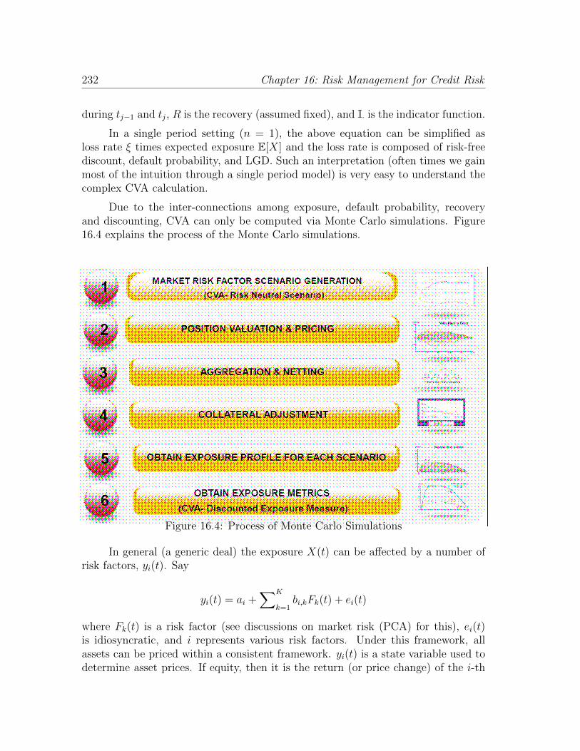
232 Chapter 16: Risk Management for Credit Risk
during tj−1 and tj, R is the recovery (assumed fixed), and I· is the indicator function.
In a single period setting (n = 1), the above equation can be simplified asloss rate ξ times expected exposure E[X] and the loss rate is composed of risk-freediscount, default probability, and LGD. Such an interpretation (often times we gainmost of the intuition through a single period model) is very easy to understand thecomplex CVA calculation.
Due to the inter-connections among exposure, default probability, recoveryand discounting, CVA can only be computed via Monte Carlo simulations. Figure16.4 explains the process of the Monte Carlo simulations.
Figure 16.4: Process of Monte Carlo Simulations
In general (a generic deal) the exposure X(t) can be affected by a number ofrisk factors, yi(t). Say
yi(t) = ai +∑K
k=1bi,kFk(t) + ei(t)
where Fk(t) is a risk factor (see discussions on market risk (PCA) for this), ei(t)is idiosyncratic, and i represents various risk factors. Under this framework, allassets can be priced within a consistent framework. yi(t) is a state variable used todetermine asset prices. If equity, then it is the return (or price change) of the i-th

CVA – Credit Value Adjustment 233
asset as described in Chapter 4. If interest rates, then it could be one of severalfactors such as: r(t) = ym(t)+ym+1(t)+· · ·+ym+h(t) assuming h factors that explainthe interest rate. Then a bond valuation model can be used to price risk-free bonds(such as Vasicek in Chapter 4) or risky bonds (such as the Jarrow-Turnbull modelin Chapter 13).1 This is step 2.
Step 3 is to aggregate all positions into a portfolio. Apparently the exposure atany time t, X(t), is a result of valuations of all assets owned and owed (netting). Step4 is related to risky funding, which is to incorporate liquidity risk (to be discussedlater). Step 5 is simulations and step 6 is taking the average.
Take the above swap as an example. Say the interest rates are results of atwo-factor model (see market risk). Then we evaluate fixed leg and floating leg(evaluation) to get exposure.
16.4.2 CCDS (contingent credit default swap)
Given that CVA is now formally incorporated in valuation, it is proposed that CVAto be securitized. This is CCDS. It is IRS + CVA. That is, the floating leg of aCCDS is the loss due to default of the IRS counterparty. As a result, CCDS is aperfect hedge to CVA.
WWR (wrong way risk) In general, the exposure with a counterparty is notindependent of the counterparty’s credit quality. Wrong Way Risk is cases wherethe exposure increases when the credit quality of the counterparty deteriorates – i.e.exposure tends to be high when PDs are high.
There are two types of WWR:
• General WWR: the counterparty’s credit quality is for non-specific reasons cor-related with macroeconomic factors which also affect the value of the deriva-tives (e.g. correlation between declining corporate credit quality and high (orlow) interest rates causing higher exposures
• Specific WWR: future exposure to a specific counterparty is highly correlatedwith counterparty’s PD. (e.g. a company writing put options on its own stock,derivatives collateralized by own shares)
WWR quantification is still an open challenge other than the self referencingspecific WWR due to:
• Difficulty to separate statistical noise from systematic correlation
1Jump intensities can also be functions of the factors.
234 Chapter 16: Risk Management for Credit Risk
• Challenge of dynamic forward looking adjustment to historical calibration
16.4.3 CVA Hedging
As CVA having become a real cost to trading desks, the hedging of CVA has becomean important task as the value of CVA is now part of the P&L of the trading desk.The hedges of the CVA incorporate hedges of the market risk factors driving theexposures and hedges of the credit spreads of the counterparties. As in any hedging,correlation among different risk factors is usually the most important feature eval-uating CVA. Empirical evidence has suggested that convexity and cross-convexity(gamma and cross-gamma) plays an important role in evaluating CVA, especiallywhen the changes in spreads and exposures are large.
If the bank marks to market its CVA and the bank does not hedge it, it willexperience P&L (and earnings) volatility. More importantly, in a trending or dete-riorating credit market environment, the bank could suffer a substantial cumulativeloss. The risk management of CVA requires dynamic rebalancing of the hedges.When counterparty exposures and credit spreads of the counterparties are large andvolatile, rebalancing requirements can be intense and costly.
In general, changes in the exposure can be hedged by taking positions on themarket risk factors that drive the exposure, but the hedging for its own credit spreadis more challenging to hedge. The systematic risk component can be hedged. Thebank-specific, idiosyncratic risk component is more difficult to hedge.
The ISDA Master Agreement lists two different tools to reduce exposure:
• Collateralization, the right of recourse to some asset of value that can be soldor the value that can be applied in the event of default on the transaction
• Close-out Netting rules, which state that if a default occurs, multiple obliga-tions between two parties are consolidated into a single net obligation
16.4.4 CSA (credit support annex)
Counterparty credit risk can also be mitigated by margining practice through incor-porating Credit Support Annex (CSA agreements). A CSA provides credit protec-tion by setting forth the rules governing the mutual posting of collateral.
CSAs are used in documenting collateral arrangements between two partiesthat trade privately negotiated (over-the-counter) derivative securities. The tradeis documented under a standard contract called a master agreement, developed by

CVA – Credit Value Adjustment 235
the International Swaps and Derivatives Association (ISDA). The two parties mustsign the ISDA master agreement and execute a credit support annex before theytrade derivatives with each other.
In addition to executing the ISDA master agreement and credit support annex,issuers must implement proper resolutions that give authorization to execute anyderivative transactions. Each issuer must also obtain an opinion from its respectivelegal counsel about whether both parties can enter into swap transactions. Issuersmust also ensure that such contracts are binding and enforceable, and obtain finalcredit approval from a bank.
ISDA Credit Support Annex (CSA)
• Permits posting one or several types of collateral with periodic rebalancingand interest paid by the receiving party based on collateral currency and type
• Permits thresholds, minimum transfer amounts, and rounding (to reduce op-erational costs)
• A new standard form of CSA (SCSA) is in development which will reduce thecomplexity due to the collateral type switch options embedded in traditionalCSA
• Fully collateralized counterparty is counterparty with a perfect CSA all thresh-olds, minimum transfer amounts, and rounding are zero, with daily rebalancing
• If the market moves against the trade and CSA is in place, massive additionalfunding will be required immediately to post collateral
• In the absence of CSA, expected future losses may cause immediate crisis ofconfidence causing creditors to pull funding from the firm
Key exposure / CVA affecting CSA terms include:
• Margin call frequency
• Threshold and Minimal Transfer Amount (MTA)
– At the end of period (day, week, etc.), if trade MTM value exceeds athreshold, collateral must be posted.
– Exposure is to the threshold plus the market moves between default andliquidation
– Symmetry and currency (one-way-in, one-way-out, two way)

236 Chapter 16: Risk Management for Credit Risk
• Initial Margin (IM): only affects claims at default and close-out
Clearing houses mitigate risk via netting, collateralization and reassignmentof contracts. Clearing houses charge initial and variation margins to make neededcash available in the event of a default. Furthermore,
• If that proves insufficient, coverage comes from backers of clearing house andequity of the firm itself
• Reassignment of contracts prevents losses due to market impact. But in areal crisis, reassignment might fail Another approach to risk mitigation is toinclude break clause (a.k.a, additional termination events)
• Contract can be close-out at replacement value if the counterpartys ratingdrops
• Contract can be closed out at market value prior to maturity
• Issues
– What exactly is replacement value?
– How is closing out of a swap early any different from entering into thereversing swap?
– By forcing a closeout upon a rating change, are you decreasing counter-party risk while increasing systemic risk?
– What if the market is illiquid?
16.4.5 Counterparty Credit Risk (CCR) as Market Risk
If CCR is actively managed and hedged, it is appropriate to treat CCR as part ofmarket risk. CCR can be incorporated in the trading book by adding to the tradingbook one defaultable exotic virtual trade per counterparty. For each counterparty,the virtual trade is defined according to:
• if the counterparty has not defaulted by time t , the virtual trades value attime t is equal to −CV A(t)
• no cash flows occur unless the counterparty defaults
• at the time of the counterpartys default at time τ , the bank pays a single cashflow equal to LGD multiplied by exposure, and the trade terminates

CVA – Credit Value Adjustment 237
16.4.6 Counterparty Credit Risk (CCR) as Credit Risk
Many banks do not actively manage CCR, but hold this risk to the portfolio matu-rity. For such banks, joint treatment of market risk and CCR may not be appropri-ate. Note that the time horizon used for market risk calculations is usually short,which can be justified only if the risk is actively managed. Hence, treating CCR ascredit risk (jointly with the banking book) may be more appropriate for such banks.
A primary challenge in treating CCR as credit risk is uncertain nature ofcounterparty credit exposure. Very often, this challenge is overcome by using loanportfolio models with deterministic loan equivalent exposures that are calculatedfrom counterparty exposure distributions.
16.4.7 Counterparty Credit Risk (CCR) Capital under BaselII & III
CCR capital under Basel II (BCBS, 2006) is treated as credit risk
• For default scenarios, asymptotic single risk factor (ASRF) model is used (seeGordy, 2003).
• Capitalization of no-default scenarios (credit migration risk) is done via cali-brating a maturity adjustment (MA) factor to a MTM credit risk model, sim-ilar to KMV Portfolio Manager and consistent with the ASRF model (BCBS,2004).
Basel III (BCBS, 2010) treats CCR in a mixed way:
• Default capital charge treats CCR as credit risk via ASRF framework (similarto Basel II, with minor changes).
• MA factor (same as in Basel II i.e., credit risk treatment) is still used forcapitalization against credit migration losses.
• A new CVA capital charge is used to capitalize against CVA losses due tocredit spread changes (EE is assumed to be fixed). CVA capital charge treatsCCR as stand-alone market risk
16.4.8 CVA Capital Charge and Basel III
Counterparty Credit Risk (CCR) is one of the primary focus points of Basel III(BCBS, 2010). Credit Valuation Adjustment (CVA) is part of the regulatory capital

238 Chapter 16: Risk Management for Credit Risk
calculations for CCR under Basel III. In addition to default capital charge, bankswill be required to calculate a CVA capital charge.
Default charge capitalizes against losses from counterparties defaults. CVAcharge capitalizes against losses from CVA increases for surviving counterparties.
Basel III motivation of CVA capital charge.
“Roughly two-thirds of CCR losses were due to CVA losses and only about one thirdwere due to actual defaults. The current framework addresses CCR as a default andcredit migration risk, but does not fully account for market value losses short ofdefault.”
Basel III CVA Capital Charge
CVA capital charge is calculated for the entire portfolio of OTC derivatives andallowable CVA hedges (securities financing transactions (SFT) are not included).Allowable CVA hedges include single-name and index credit default swaps (CDS)contracts (allowable hedges are removed from market risk calculations).
Two methods are available: advanced (based on simulations) and standardized(based on formula)
• Banks with Internal Models Method (IMM) approval for CCR and approvalto use the market risk internal models approach for the specific interest-raterisk of bonds must use advanced method
• All other banks must use the standardized method
16.4.9 Advanced CVA Capital Charge
Advanced CVA charge is based on stand-alone CVA VaR which is a VaR chargeresulted from CVA. Usually Monte Carlo simulations are used to compute this quan-tity. This is similar to the calculation of credit exposures that can only be simulated.In simulations, changes of credit spreads for all counterparties and of credit indexesare simulated for a 10-day horizon using internal models on a stand-alone basis. Foreach scenario, changes of CVA for each counterparty and those of MTM values ofallowable hedges are calculated. For each scenario, changes of counterparty CVAsand those of hedge MTMs are aggregated across counterparties and hedges, result-ing in a distribution of changes in portfolio-level hedged CVA. Then 99% VaR is

Risky Funding 239
calculated from the simulated distribution of changes in the portfolio-level hedgedCVA.
Next, CVA capital charge is obtained from CVA VaR according to marketrisk rules (BCBS, 2009). The calculation must include Stress VaR, but excludeIncremental Risk Charge (IRC).
Standardized CVA Capital Charge
Standardized CVA charge under Basel III, K, is calculated according to a formula:
K = β√TN−1(q)
where
β2 =
[1
2
∑N
i=1wi
(XiMi −B∗iM
(h)i
)− wB∗M (h)
]2
+3
4
∑N
i=1w2i
(XiMi −B∗iM
(h)i
)2
,
T = 1 year is the time horizon and q = 99.9% is the confidence level, wi is standard-ized “weight” based on credit rating of counterparty i, Xi and Mi are the exposureat default (EAD) and is effective maturity respectively for counterparty i, B∗i and
M(h)i are the discounted notional and the maturity of single-name CDS hedge re-
spectively on counterparty i, and B∗ and M (h) are the discounted notional and thematurity of index CDS hedge.
16.5 Risky Funding
The recent 2007-8 crisis has revolutionized what financial modeling has long believedin – the law of one price, a result achieved by no-arbitrage. No-arbitrage was thebasic principle Black and Scholes used to derive their option formula. No-arbitragegave birth to risk-neutral pricing that has dominated the quant finance area for halfof a decade. No-arbitrage guarantees the law of one price.
We should recall how Black and Scholes derived the pricing equation (i.e.the partical differential quation). This is known as “price by replication”. In otherwords, Black and Scholes taught us that the price of any security is equal to its cost ofhedging (or replicating). Later on, this was shown as the Martingale RepresentationTheorem (a.k.a. self-financing, which is the base of no-arbitrage). However, toachieve this result, one must have the same borrowing and lending rate. Well, this

240 Chapter 16: Risk Management for Credit Risk
is not a problem under no-arbitrage, since the only rate relavent under no-arbitrage(or risk-neutral pricing) is the risk-free rate.
Until the 2007-8 crisis, the paradigm seemed to work just fine. Everythingis calibrated to LIBOR which is regarded as the risk-free rate by the investmentcommunity. The crisis changed everything. During the crisis, deals that were safelycollaterized were priced very differently (at much higher prices) from those that werenot safely collaterized (either under-collaterized or un-callaterized). Buyers did nothave faith in their counterparties’s ability to fund the transactions (if the deals wereunder- or un-collaterized) and consequently demanded for lower prices. LIBOR andOIS rates started to diverge and LIBOR was no longer the risk-free rate anymore.This is the issue called Risky Funding.
There has not been any solution yet for this problem. Proposals have beenprovided but no conclusion has been drawn. This is a still very live and challengingproblem.
16.6 Appendix
16.6.1 Poisson Process of Defaults
A Poisson process, named after the French mathematician Simon-Denis Poisson(1781 - 1840), is the stochastic process in which events occur continuously andindependently of one another. The Poisson process is a continuous-time process: itsdiscrete-time counterpart is the Bernoulli process.
A homogeneous Poisson process is characterized by a rate parameter λ, alsoknown as intensity, such that the number of events in time interval (t, t+ τ ] followsa Poisson distribution with the associated parameter λτ . This relation is given as:
Pr[N(t+ τ)−N(t) = j] =(λτ)je−λτ
j!(16.4)
Hence,
Pr[N(t+ τ)−N(t) = 0] = e−λτ (16.5)
The Poisson process is an ideal way to model unexpected defaults as an eventoccurs with no prior memory. (16.5) describes the probability of no default between(t, t+ τ ]. The mean and variance of a Poisson distribution are:

Appendix 241
E[j] = V[j] = λτ (16.6)
Exponential Distribution
If an event occurs with a Poisson distribution, then it can be shown that the time ofthe event occurring follows an exponential distribution. The exponential distributionis (with parameter λ):
f(x) = λe−λx (16.7)
Hence, its cumulative density function is:
Pr[x < τ ] = F (τ)
=
∫ t
0
f(x)dx
= 1− e−λτ
(16.8)
or
Pr[x > τ ] = 1− F (τ)
= e−λτ(16.9)
which is the survival probability when t represents the default time. When the timeinterval is small, we can use Taylor’s series expansion to approximate the survivalprobability as:
Pr[x > τ ] = e−λτ ≈ 1− λτ (16.10)
or the default probability λτ . The mean and variance of the exponential distributionare:
E[x] =
1
λ
V[x] =1
λ2
(16.11)
Note that the Poisson process has no memory. Hence, the exponential distri-bution has the following property:

242 Chapter 16: Risk Management for Credit Risk
Pr[x > s+ t|x > s] =e−λ(s+t)
e−λs
= e−λt
= Pr[x > t]
(16.12)
In plain words, what this means is that the expected wait time (till the event)has nothing to do with how long one has waited. The event is not expected tohappen sooner even though you have already waited for a long time.
We compute survival probabilities when we model default. The survival prob-ability between now and some future time T if we adopt the Poisson process (i.e.default time τ) for defaults is:
Q(t, T ) = Pr[τ > T ] = Et[Iτ>T] = e−λ(T−t) (16.13)
where I is an indicator function.

Appendix 243
16.6
.2E
qu
ati
on
13.2
3
For
the
firs
tye
ar,
whic
hco
nta
ins
four
quar
ters
,n
=4
and
we
hav
e:
x1
=x
0+
0.6p
1+
(1−p 1
)x0
x2
=x
0+
0.6p
1+
(1−p 1
)x1
x3
=x
0+
0.6p
1+
(1−p 1
)x2
x4
=x
0=−
0.00
0225
Subst
itute
recu
rsiv
ely
intox
4to
get:
0=
0.6p
1+
(1−p 1
)
−0.0
0022
5+
0.6p1+
(1−p1) −0
.000225+
0.6p1+(1−p1)[ −0
.000225+
0.6p1−0.000225(1−p1)
1.0125
]1.0125
1.0
125
1.
0125
and
solv
efo
rp 1
=0.
0003
75or
3.75
bas
isp
oints
.

244 Chapter 16: Risk Management for Credit Risk

Part IV
Liquidity Risk


Chapter 17
Liquidity Quantification
17.1 Introduction
The default of Lehman Brothers Inc on September 15, 2008 marked the unprece-dented crisis in the global history. This crisis differed from the previous ones inthat:
• it caused the largest bankruptcy in the U.S. history (over $600 billion)
• it caused a global recession
• it recorded the longest recession in the U.S. history
• it started global awareness on regulation
And the trigger of Lehman default is liquidity. While the cause of the crisis, justline any other, is a bubble burst in the real estate market, and frauds committed inmaking unjust mortgage loans (so called subprime loans), the snowball of one defaultof Bear Sterns has been unprecedented and liquidity driven. As a result, liquidityrisk management has been the focal point of regulation reform in EU (Basel) andthe U.S. (Dodd-Frank).
During the last financial crisis (known as the liquidity crisis), a large numberof liquidity-squeezed events had occurred. These incredible events had caused WallStreet to consider abandoning its long proud tradition – marking to market. Foras long as Wall Street has existed, it has prided itself in respecting the marketprices. Wall Street had always regarded market prices to be a reflection of collectivewisdom of the entire investment community. The fact that there is a price reflectsan equilibrium. Wall Street is proud to be able to take the full advantage of such

248 Chapter 17: Liquidity Quantification
equilibriums and develop tools that are consistent with market prices. But duringthe crisis, such a belief had been put under a strong test. Here are some famousexamples.
17.1.1 Some Liquidity Squeeze Examples
Lone Starr-Merrill Lynch Deal
On July 28, 2008, a Monday, as the crisis of subprime gradually unfolded, MerrillLynch, in realizing huge toxic portfolios it owned, would like to sell a particularsubprime portfolio that had a face value of $31 billion to a private equity fundowned by Mr. Lone Star. The purchase price was rumored to be 22 cents on thedollar – a 78% discount. On top of that, Merrill Lynch needed to buy back anydefaulted asset in the portfolio. In other words, Merrill Lynch was implicitly sold aCDS (for free) to Star, which was worth about 15 cents on the dollar. As a result,Merrill Lynch sold Lone Star a portfolio of financial assets at a discount of 93%!
According to Reuters, the deal had prompted Merrill Lynch to write down allof its toxic assets by at least 75%, an unprecedented price discount seen on WallStreet.
Bear Stearn-JP Morgan Deal
On June 22, 2007, the problems of the two subprime portfolios managed by BearStearns Asset Management (BSAM) – Bear Stearns High-Grade Structured CreditEnhanced Leveraged Fund and Bear Stearns High-Grade Structured Credit Fund,started to surface. Its CEO James Cayne initially wanted to keep the two fundsseparate from the main Bear Stearn bank (as how deals are usually done on WallStreet – so called special purpose vehicle, or SPV). Yet the pressure from the in-vestors and the government forced Bear Stearns to take over. As losses graduallyunfolded, Richard A. Marin, a senior executive at Bear Stearns Asset Managementresponsible for the two hedge funds, was replaced on June 29 by Jeffrey B. Lane, aformer Vice Chairman of rival investment bank, Lehman Brothers.
On March 14, 2008, Bear Stearns finally reached to a point where it could nolonger operate. Either someone would have to buy it or else it would face liquidation.The Fed called in JP Morgan for the bail out. The price was at $30 per share onMarch 14, a Friday. After a weekend-long investigation and evaluation of Bear’sassets, JP Morgan offered $2 per share. Bear rejected and accused JP Morgan ofexploiting the liquidity situation. In fear of a bank run that Bear’s bankruptcy couldhave caused, the Fed yielded to JP Morgan for liquidity concern by agreeing a $30

Understanding Liquidity and Liquidity Risk 249
billion loan to J.P. Morgan. The final deal was $10 per share.
It is a consensus that Bear’s default would have been an economic consequence(that is, they lost money in their investments). Yet the bailout amount (from $2 pershare to $10 per share) is undoubtedly a consequence of a liquidity squeeze. Theliquidity discount here is 80%!
Other Examples
In addition to these two unprecedented liquidity events, there have been numerousexamples during the crisis period where asset prices were largely compressed due tourgent needs to unwind those positions (clear evidence of liquidity squeeze).
17.2 Understanding Liquidity and Liquidity Risk
Liquidity standards aim to ensure that a bank is able pay its liabilities on time byholding enough highly liquid assets that could be quickly converted to cash.
Ever since the recent financial crisis, liquidity has been the centerpiece inmany regulations. Basel III explicitly calls for liquidity regulations (LCR or Liq-uidity Coverage Ratio, and NSFR or Net Stable Funding Ratio). Dodd-Frank Sec-tion 165 directs the Federal Reserve Board (FRB) to establish heightened liquid-ity standards for both bank holding companies with over $50 billion in assets andFSOC-designated non-bank systemically important financial institutions (coveredcompanies).
17.3 How to Measure Liquidity
Liquidity is generally understood in the following three areas:
• market microstructure liquidity
– volume
– bid-offer spread
– price movement
• banking liquidity
– Basel III – LCR and NSFR
250 Chapter 17: Liquidity Quantification
– Dodd-Frank – to be determined
• accounting going concern liquidity (whether or not a firm has enough cash (orliquid assets that can turn into cash quickly) to pay of its expenses)
Accountants for centuries have played an essential in diagnosing the liquidityhealthiness of a firm. The so-called “going concern audit” is an audit opinion to tellthe stock holders if a firm is likely to survive through the next year (going concernis an annual audit).
In five accounting ratio groups – productivity (e.g. ROE), profitability (e.g.profit margin), market (e.g. PE ratio), efficiency (e.g. turnover ratios), and liquidity(acid ratio), liquidity measures take into account of if the firm has enough cash forthe coming year to pay for its short-term liabilities.
This is the most conservative measure of liquidity as only cash (or the ex-tremely marketables) is considered. Other assets that can be liquidated to pay forthe liabilities are not considered. However, if each asset can be measured with aliquidity discount, then the firm can remain liquid as long as the total asset valueis enough to cover the short-term liabilities. However, doing so requires a model toevaluate each asset with a liquidity discount.
17.4 Liquidity and Liquidity Risk
Liquidity is a static measure of how much should there be enough liquid assets (suchas cash) for a firm to survive in a specified period (usually a year). Liquidity risk,on the other hand, refers to future liquidity needs and the likelihood that the firmmay not be able to meet the needs. In other words, liquidity risk is about futureliquidity shortfalls. The following summarizes the difference between liquidity andliquidity risk:
• liquidity is static and liquidity risk is dynamic (probabilistic)
• liquidity is single period and liquidity risk is multiple periods
• liquidity risk requires models and liquidity does not
The diagram below depicts liquidity shortfalls (a.k.a. liquidity gaps). In thediagram the demand for liquidity on the asset side exceeds the supply of liquidity onthe liabilities side. Hence there is a liquidity gap. Liquidity risk is to study futuresuch gaps and compute the impact of these gaps.

How to Measure Liquidity Risk 251
Figure 17.1: Liquidity Risk Gap
17.5 How to Measure Liquidity Risk
17.5.1 Liquidity Discount as a Put Option
Liquidity discount occurs as supply reacts more sensitively to economy than demanddoes in a non-linear fashion. Liquidity discount reaches the extreme as demandreaches its maximum capacity. Figure 1 depicts this general idea. In Figure 1, weassume that demand and supply of a financial asset jointly determine the equilibriumprice of the asset at any given time. The economy is represented by a single statevariable (say wealth) symbolized by V . As the economy grows, the supply curvemoves to the right and so does the demand curve. To derive the liquidity discountmodel, we must assume that supply grows faster than demand does in that lesselastic demand function is the main reason to cause price discount.
As a result, the growth of economy results in an increased equilibrium quantityand a lower price. In the diagram, we assume that the demand is totally insensitive toeconomy growth and it has a maximum capacity at Q∗. Clearly, our model requiresonly demand be less sensitive to supply and such an exaggerated demonstration isjust for the purpose of easy exposition. At the maximum capacity of the demandfunction, the quantity can no longer increase and equilibrium can only draw theprice down.
In the diagram, the vertical axis represents price (by S) and the horizontal axisrepresents quantity (by Q). We let the liquidity-constrained price be S∗. In a usualsituation, S = S∗. In a liquidity-squeezed situation (represented by the situation

252 Chapter 17: Liquidity Quantification
S = S*
S ↓ S*
S ↓ S*
Q* ← Q
Q = Q*
V ↑
Figure 17.2: Demand-Supply Analysis of Liquidity Discount
where demand reaches its maximum capacity Q∗), S > S∗. Liquidity discount inthis setting is defined as the impact of the slower demand reaction (than supply) andbecomes dramatic as the maximum is approached. Based upon the above diagram,we can draw the following conclusion depicted in Figure 2.
On the left of Figure 17.3, we depict the relationship between the economy(represented by, say wealth V ) and perfectly liquidity price S. As shown in Figue17.2, this is a downward sloping curve. To be shown later, the curvature of S in Vmust be convex in order to obtain liquidity discount. If the relationship is linear(under which Q∗ cannot exist), then there can be no liquidity discount. ,
On the right, we depict the relationship between the perfectly liquidity price Sand the liquidity-constrained price S∗. The line ABC is a 45-degree line on which theilliquid price is equal to the liquid price. At point B where the quantity reaches itsmaximum capacity Q∗ the illiquid price starts to decrease rapidly due to problemsin liquidity and bends over toward point D. Again, the linear result (by BD line)is just a demonstration. In the next section where we derive the formal model, thegraph between points B and D is not linear and has a reflection point.
From the diagram where discount is depicted linearly, it can be seen thatliquidity can be explained by a put option. That is,
S∗ = S − put (17.1)
In the next section, we demonstrate that this is not a simple put due to con-vexity requirements. But intuitively, the simple put explanation serves the purpose

How to Measure Liquidity Risk 253
S
V S*
A
B (Q = Q*)
C
D
Figure 17.3: Liquidity Discount as a Put
well and can even be used as an approximation, which has already been discussed inthe industry. What is offered in this paper is an equilibrium model that is consistentwith the Merton model widely used in modeling credit risk. While we do not linkour liquidity model yet to credit risk in this paper, it is quite straightforward to doso.
Take the Black-Schole put formula as an example:
put = e−rTK[1−N(d2)]− S[1−N(d1)] (17.2)
where
d1 =lnS − lnK + (r + 0.5σ2)T
σ√T
d2 = d1 − σ√T
Assuming S = 100, K = 120, r = 0.04, σ = 0.3, T = 1, the discount forliquidity is $21.88, which means that the illiquid price is 100−21.88 = $78.12. Notethat K is a parameter in the model that decides critically the value of the discount.The larger is K, the more severe is the discount. When K is 0, then there is nodiscount. As K approaches infinity, the value of discount is approaching $100 andthe illiquid price becomes 0.
In this section, the demonstration is intuitive but not realistic. In reality, the

254 Chapter 17: Liquidity Quantification
left and the right panels are related. In other words, how the liquidity price reactsto the economy affects the magnitude of liquidity discount. Furthermore, it is notlikely to know the exact amount of Q∗. In the next section, we endogenize therelationships amount the economy V , the perfect liquid price S, and the liquidity-constrained price S∗. We let the liquid price be a convex function of the economyand derive the illiquid price directly. In doing so, we arrive an equilibrium withoutthe specification of Q∗.
17.5.2 The Model
In this section, we develop a formal pricing model for illiquidity which is defined asinability to transact. Inability to transact is the exact description of Figure 17.2 inwhich lack of demand leads to no transactions. In a perfect world where the Black-Scholes model holds, transactions can take place at any time and hence investorscan trade securities and rebalance their portfolios continuously. When transactionsare not permitted to be continuous, it presents an extra risk born by the buyer andhence the buyer, in return, should ask for compensation and lower the price of thesecurity.
Once continuous trading is not allowed, market is not (dynamically) completein the Duffie-Huang sense (1985) and the resulting model is not preference-free. As aresult, one must adopt a utility function to gauge the magnitude of the risk premium.We first present a model with the quadratic utility so the standard CAPM can beused. It is straightforward to extend the model to a broader class of utility functions.Using a more complex utility function is certainly better in terms of explaining thereality and providing model flexibility but it loses the closed-form CAPM formula.
The price of an arbitrary security at current time t when no trading is alloweduntil a future time T can be priced by the most fundamental discounted cash flowmethod:
X(t) = e−ξ(T−t)Et[X(T )] (17.3)
where X(t) is the cash flow of an arbitrary security at time t, Et[·] is the conditionalexpectation taken at time t, and ξ is the (continuously compounded) risk-adjustedreturn for the security. Such a discounted cash flow method requires further model-ing substances in order to be operational.
To build an explicit model for (17.3), we first assume the Black-Scholes/CAPMmodel where the underlying economy (represented by a single state variable, saywealth) obeys the following log normal process:

How to Measure Liquidity Risk 255
dV
V= µdt+ σdW (17.4)
where W (t) is the standard Wiener process and µ and σ are (continuous time) meanand standard deviation of the return of the state variable V .
A perfectly liquid price, S, is a contingent claim on the state variable. Theassumption of liquidity discount we make in this paper indicates that S must be amonotonic function in wealth V . In a theorem we shall prove later, the functionmust be convex in order to arrive at liquidity discount. There are a number ofways to construct such an explicit function. For simplicity, we choose a functionthat imitates a put option (as opposed to an arbitrary polynomial function) for thefollowing reasons. First, the maturity parameter in the put option can be madeequal to the liquidity discount horizon. This provides an extreme convenience inmodeling liquidity discount. Secondly, there is a closed form solution for the priceof a perfectly liquid asset, which allows us to compare with the price of an equalasset but constrained by liquidity. Lastly, the strike price in the put function ideallycharacterizes the strength of the liquidity squeeze. The higher is the strike price,the stronger is the liquidity discount and the zero strike price ideally representsperfect liquidity. However, the use of put function does suffer from one drawback.It exists a maximum value for the liquid stock price (at the strike level), whichcould be unrealistic as economy contracts the price of the security could becomeunboundedly high. Fortunately, this is the situation where the liquidity discount issmall and hence the impact would be small.
Given that S is the price of a security that can be continuously traded, it canbe easily computed with the Black-Scholes model when its payoff for a fixed timehorizon (time to maturity) mimics a put:
S(t) = e−r(T−t)Et[S(T )]
= e−r(T−t)Et[maxK − V (T ), 0]= e−r(T−t)KN(−d−)− V (t)N(−d+)
(17.5)
where K is the strike price that reflects the strength of the liquidity squeeze, Et[·]is the risk-neutral expectation, and
d± =lnV (t)− lnK + (r ± 1/2σ2)(T − t)
σ√T − t
Note that the adoption of the put payoff is just a convenience to incorporateconvexity. Due to the fact that the liquidity-constrained price does not have a

256 Chapter 17: Liquidity Quantification
closed-form solution (except for the extreme cases), we implement a binomial modelto approximate this Black-Scholes result. For the remainder of the paper, when werefer to the Black-Scholes model, it is actually the binomial approximation.
We also note that although the liquidity discount model has no closed formsolution, the binomial implementation is actually better in that the model can thenbe easily augmented to include credit risk proposed by Chen (2002), and Chen,Fabozzi, Pan, and Sverdlove (2008). In this broader model, interactions betweenliquidity and credit risks can be studied.
Let S∗ be the liquidity-constrained price where trading of the security is notpermitted until time T . Equation (17.3), as a result, can be replaced with thefollowing equation:
X(t) = e−ξ(T−t)Et[f(V (T ),Θ), 0] (17.6)
where Θ represents other parameters needed for the model, X(t) is either S or S∗
depending if the equation is used for an instantaneous period or a longer time period,respectively. Note that in an instantaneous period, the physical expectation as in(17.6) is identical to the risk-neutral expectation (details to be explored later inTheorem 1) and hence (17.6) provides the solution to the liquid price. The expectedreturn, ξ, must follow the Capital Asset Pricing Model (CAPM).
Note that S and S∗ are identical securities with just one difference: S∗ cannotbe transacted (or hedged) until time T . The purpose of the paper is to derive theprice difference between S and S∗. We shall prove that S∗ < S and this is the modelof liquidity discount. As we shall demonstrate in an analysis that such discount canbe substantial, even under very reasonable assumptions.
We begin our modeling of liquidity discount with the standard CAPM. Notethat the Black-Scholes model is consistent with the standard CAPM as follows:
ξ = E[dX
X
]= rdt+ η
[E[dV
V
]− rdt
](17.7)
where r is the risk-free rate and
η =∂X
∂V
V
X(17.8)
is the elasticity of the state contingent claim with respect to the underlying economicstate variable (similar to an option on its underlying stock). Note that this resultis exact only in continuous time. Black and Scholes (1973) prove that the option

How to Measure Liquidity Risk 257
price is a CAPM result with the underlying stock as the market. Note that η = βas shown in the following:
β = K[dX
X,dV
V
]/V[dV
V
]=V
X
K[XV dV, dV ]
dV
=V
XXV
= η
(17.9)
where XV = ∂X/∂V . Re-writing (17.7) in discrete time for a small interval h, wehave:
E[X(t+ h)]
X(t)= (1 + rh) + β
[E[V (t+ h)]
V (t)− (1 + rh)
](17.10)
As a result, we can derive a pricing model for the security as:
X(t) =1
R(t, t+ h)(E[X(t+ h)]−XV E[V (t+ h)]−RV (t)) (17.11)
where R(t, T ) = 1 + r(T − t) ≈ er(T−t). This result provides an alternative proof ofthe CAPM argument by Black and Scholes. Note that
XV =K[X(t+ h), V (t+ h)]
V[V (t+ h)]
= β$
(17.12)
is the “dollar beta” (that is, delta is dollar beta). Hence, (17.11) is also an alternativederivation to Jensen’s model (1972).
It is important to note that CAPM holds only under one of the two assump-tions: quadratic utility for the representative agent in the economy or normalityfor the returns of the risky assets. Consequently, the above CAPM result holds inthe Black-Scholes model without any utility assumption must be due to the factthat option returns and stock returns are both normally distributed. It is clearthat the stock return is normally distributed, as equation (17.4) postulates. Theoption return is normally distributed only under continuous time. This is becausein continuous time, the option value is linear in stock and must follow the samedistribution of that of the stock and hence its return is normally distributed.

258 Chapter 17: Liquidity Quantification
In a discrete time where h is large, the option return is no longer normallydistributed and the equation (17.11) can no longer hold without the assumptionof quadratic utility that guarantees the validity of the CAPM quadratic utilityfunction. The quadratic utility function is a bad assumption in that it has the wrongsign for the relative risk aversion. However, fortunately, the liquidity discount modelwe derive in this paper suffers very little from the second order effect of the utilityfunction. All the model requires is that investors are risk adverse.
Under quadratic utility, CAPM holds for all securities. Hence, equation (17.11)holds for an h that is not infinitesimally small as follows:
X(t) =1
R(t, T )(E[X(T )]− β$E[V (T )]−R(t, T )V (t)) (17.13)
where R(t, T ) = er(T−t) and the dollar beta is computed, for any T , as:
β$ =K[X(T ), V (T )]
V[V (T )](17.14)
Equation (17.13) is the main result of our model. It states that under quadraticutility, all assets must follow CAPM in determining their values. What we shalldemonstrate is that when liquidity discount is present, the value computed by equa-tion (17.13) is less than the perfectly liquid price computed by the Black-Scholesmodel.
To derive our liquidity discount model, we shall show first that if the rela-tionship between the economy (represented by the state variable V ) and the liquidprice (S) is linear, then the liquidity discount is nil. Then we show that liquiditydiscount can exist only if the relationship between the economy and the liquid priceis convex.
Theorem 1 When the payoff is linear, then liquidity discount is nil.
In continuous time, there are only two states in every infinitesimal time step(as described in Duffie and Huang (1985)) and hence no liquidity discount can exist.This indicates that if trading is continuous then at each infinitesimal step the payoffis linear and as a result Theorem 1 holds. In other words, continuous tradingbreaks up a fixed time horizon into small infinitesimal time steps, each of which isa linear payoff and hence liquidity discount does not exist. In the next section, weshall demonstrate this property in a numerical example and Theorem 1 is explicitlydemonstrated.
Theorem 2 in the following proves that if the payoff is not linear and is convex,then the equilibrium price is always less than the linear price which, by Theorem 1,

Some Analysis 259
is the risk-neutral price where continuous rebalancing is possible.
Although a general proof with any form of convexity is not available, a proofbased upon the binomial model that is consistent with our formulation of (17.4)is provided. In particular, as any three points define the convexity, we use a twoperiod binomial model for the proof. It can be referred that with more points (moreperiods) in the binomial model, the proof stays valid.
Theorem 2 If the payoff is not linear and convex, then Xcvx(t) < X lnr(t) whereX lnr(t) is defined in [Theorem 1] and identical to S(t) which is the perfectly liquidprice and Xcvx(t) is the same as S∗(t) which is the liquidity-constrained price.
From Theorem 1, we know that X lnr0 = S(t) as the liquid price. Here, Xcvx
0 =S∗(t) represents the illiquid price. Hence, in summary, S∗(t) < S(t) for all values offinite R(0, 2) and the theorem is proved.
Note that under linearity (between wealth and liquid price), there exists noliquidity discount, which is the same result as continuous trading. As a consequence,the price under linearity X lnr
0 is identical to the price under continuous trading S(t).Similarly, when the relationship between wealth and liquidity price is convex, thereexists liquidity discount. And the price Xcvx
0 represents the price under liquiditysqueeze, S∗(t).
17.6 Some Analysis
In this section, we provide a numerical example to demonstrate the enormity ofliquidity discount. The main model is equation (17.13). While the analysis inthis section is based upon an arbitrarily chosen set of parameter values, the resultholds in general. While equation (17.13) is closed-form, (13) needs to be computednumerically as:
β =
∑nj=1
(nj
)pj(1− p)(n−j)Vi(T )− V (T )Xj(T )− X(T )
∑nj=1
(nj
)pj(1− p)(n−j)[Vj(T )− V (T )]2
(17.15)
where
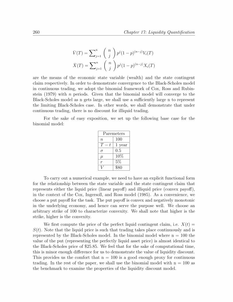
260 Chapter 17: Liquidity Quantification
V (T ) =∑n
j=1
(nj
)pj(1− p)(n−j)Vi(T )
X(T ) =∑n
j=1
(nj
)pj(1− p)(n−j)Xi(T )
are the means of the economic state variable (wealth) and the state contingentclaim respectively. In order to demonstrate convergence to the Black-Scholes modelin continuous trading, we adopt the binomial framework of Cox, Ross and Rubin-stein (1979) with n periods. Given that the binomial model will converge to theBlack-Scholes model as n gets large, we shall use a sufficiently large n to representthe limiting Black-Scholes case. In other words, we shall demonstrate that undercontinuous trading, there is no discount for illiquid trading.
For the sake of easy exposition, we set up the following base case for thebinomial model:
Paremetersn 100T − t 1 yearσ 0.5µ 10%r 5%V $80
To carry out a numerical example, we need to have an explicit functional formfor the relationship between the state variable and the state contingent claim thatrepresents either the liquid price (linear payoff) and illiquid price (convex payoff),in the context of the Cox, Ingersoll, and Ross model (1985). As a convenience, wechoose a put payoff for the task. The put payoff is convex and negatively monotonicin the underlying economy, and hence can serve the purpose well. We choose anarbitrary strike of 100 to characterize convexity. We shall note that higher is thestrike, higher is the convexity.
We first compute the price of the perfect liquid contingent claim, i.e. X(t) =S(t). Note that the liquid price is such that trading takes place continuously and isrepresented by the Black-Scholes model. In the binomial model where n = 100 thevalue of the put (representing the perfectly liquid asset price) is almost identical tothe Black-Scholes price of $25.85. We feel that for the sake of computational time,this is minor enough difference for us to demonstrate the value of liquidity discount.This provides us the comfort that n = 100 is a good enough proxy for continuoustrading. In the rest of the paper, we shall use the binomial model with n = 100 asthe benchmark to examine the properties of the liquidity discount model.

Some Analysis 261
Next we turn to computing the illiquid price, i.e. X(t) = S∗(t). We start ouranalysis with n = 1 where we demonstrate that in this case, the liquid price (whichis computed by the binomial model based upon the risk-neutral probabilities) isidentical to the illiquid price (which is computed by the CAPM based upon thephysical probabilities). In other words, when rebalancing is permitted at every nodein the binomial model, the illiquid price is identical to the liquid price.
In a one period model (i.e. n = 1), it is clear that the up and down movements
in the binomial model are u = eσ√
∆t = e0.5×1 = 1.6487 and d = 1/u = 0.6065. Thestate variable lattice and the stock payoff are given below (left and right respec-tively):
State Variable V State Contingent Claim Payoff S
131.9080
48.52
0 28.07
51.48
The risk-neutral probabilities are p = exp(r∆t)−du−d = exp(5%×1)−0.6065
1.6487−0.6065= 0.4267
and 1− p = 0.5733. The liquid price is (call): 0.5733× 51.48÷ e−5% = 28.07, as inthe above binomial tree.
The physical probabilities are p = exp(µ∆t)−du−d = exp(10%×1)−0.6065
1.6487−0.6065= 0.4785 and
1−p = 0.5215. Following (17.13), we arrive at the same exact price of $28.07 wherethe expected level of the state variable is $88.41; the dollar beta β$ is 0.6174; theexpected value of the illiquid price is $26.84; and the risk-free discount is 0.9512.
The fact that the price of the illiquid asset equals the price of the liquidasset suggests that the illiquid price is independent of the physical probability p(and also independent of µ). The reason is that in a single period binomial model,the option payoff is linear in the underlying asset and Theorem 1 applies. Thisresult is extremely crucial in our model in that once we approach continuous trad-ing/rebalancing, the binomial model suggests that the option price within a periodis linear in the underlying asset and as a result, the illiquid price must equal theliquid price the boundary condition it must satisfy by definition.
As n becomes large, liquidity discount becomes large. As in the base casewhere n = 100, the discount is substantial. The binomial value is $25.86 and theliquidity-constrained price, i.e. (17.13), is $24.47 representing a 5% discount.
To demonstrate the binomial implementation of our model, we let i be thetime index and j be the state index. At the end of the binomial lattice i = n. Ateach time i, the state j is labeled as 0 6 j 6 i. The level of the state variable, the

262 Chapter 17: Liquidity Quantification
Volatility and u and dσ 0.8 0.6 0.4 0.2u 1.083287 1.061837 1.040811 1.020201d 0.923116 0.941765 0.960789 0.980199
price of the liquid security, and the price of the illiquid security for the economy arethen labeled as Vij, Sij, and S∗ij respectively. The risk-neutral probability and thephysical probability are defined as usual and given above.
In the following, we present results when the risk preference represented bythe Sharpe ratio ranges from 0 (risk free case) to 1.6. Rebalancing frequency isrepresented by k. And k = n − 1 represents perfect rebalancing or continuoustrading (that is, for 100 periods, rebalancing 99 times in between is identical tocontinuous trading).
In the binomial model, the number of periods n must be divisible by one plusthe rebalancing frequency, i.e. k + 1, to avoid unnecessary numerical errors. In thebase case where n = 100, k can be 0, 1, 3, 4, 9, ..., 99. Take k = 3 as an example,rebalancing is allowed at i = 25, 50, and 75. At each of these times, equation (17.13)is used to compute the illiquid price at every node at the given time. Specifically, ati = 75, equation (17.13) is used to compute values at the nodes that are representedby j = 0 ∼ 75 (i.e. S∗75,0 till S∗75,75). Then at i = 50, equation (17.13) is again usedto compute values where j = 0 ∼ 50 (i.e. S∗50,0 till S∗50,50) using the prices from S∗75,0
till S∗75,75. This process repeats backwards until we reach todays price which is S∗0 .
We compute a number of liquid and illiquid prices under various scenarios.Unless otherwise mentioned, the values of the input variables are taken from thebase case. Note that liquidity discount is more severe as investors are more riskaverse. To measure the magnitude of risk aversion, we adopt the Sharpe ratio onthe underlying state variable, which is excess return scaled by the volatility. Wesimulate various degrees of Sharpe ratio from 0 (risk free case) to 1.6 with thevolatility scenarios from 0.2 to 0.8. At the risk-free rate of 5%, we obtain therequired rate of return (µ = r+λσ where λ is Sharpe ratio) from 5% (risk-free case)to 133% (λ = 1.6).
The results are summarized in Table 17.1. The top panel are binomial pa-rameter values where u = exp(σ
√∆t) and d = 1/u under n = 100. The middle
panel contains different expected returns) under different volatility scenarios foreach Sharpe ratio. The bottom panel presents physical probability values usingthe binomial formula p = [exp(µ∆t) − d]/[u − d]. Interestingly, each Sharpe ratiocorresponds to a physical probability value roughly.
Combine the information of the physical probabilities and other input values,

Some Analysis 263
µ (drift)0 0.05 0.05 0.05 0.05
0.4 0.37 0.29 0.21 0.130.8 0.69 0.53 0.37 0.211.2 1.01 0.77 0.53 0.291.6 1.33 1.01 0.69 0.37
p (physical probability)0 0.4831 0.4892 0.4963 0.5075
0.4 0.5032 0.5092 0.5163 0.52750.8 0.5232 0.5293 0.5363 0.54761.2 0.5434 0.5494 0.5564 0.56761.6 0.5636 0.5695 0.5765 0.5877
Table 17.1: Shapre Ratio and µ and p
we can then compute liquid and illiquid prices using equation (17.13). Note thatwhen the Sharpe ratio is 0, there is no liquidity discount and the liquid value equalsthe illiquid value, as proved by Theorem 1. This allows us to examine the magnitudeof the liquidity discount as a function of risk preference. Table 2 provides all theliquid (Sharpe ratio is 0) and illiquid prices. The strike price for the result is set at100 and the state variable is set at 80.
Reported in Table 17.2 are simulated liquid (Sharpe ratio is 0) and illiquidprices (Sharpe ratio is greater than 0). Note that by construction, our model forilliquid prices degenerates to liquid prices as the Sharpe ratio approaches 0. Alsoas required by the model, when continuous trading is reached (k = 99), we obtainliquid prices and risk preference does not matter (bottom panel). Liquidity discountis at maximum when no trading/rebalancing is allowed (k = 0).
To visualize the effect, we translate the values in Table 2 from dollar terms topercentage terms. In each case, the liquid price serves as the benchmark (namedBlack-Scholes value). This is the value consistent with continuous trading. Variouscomparisons are provided in Figure 17.4 and Figure 4 as follows.

264 Chapter 17: Liquidity Quantification
σ (volatility)k = 0 0.8 0.6 0.4 0.2
0 35.4303 29.0305 22.7066 16.98600.4 29.7751 25.1990 20.5670 16.27680.8 21.9833 19.2094 16.5282 14.38711.2 14.1540 12.734 11.6111 11.44281.6 7.8894 7.2781 7.0476 8.0259
k = 9 0.8 0.6 0.4 0.20 35.4303 29.0305 22.7066 16.9860
0.4 34.8789 28.6789 22.5240 16.93340.8 33.9291 28.0265 22.1478 16.80681.2 32.5311 27.0385 21.5570 16.59931.6 30.6061 25.6581 20.7160 16.2998
k = 19 0.8 0.6 0.4 0.20 35.4303 29.0305 22.7066 16.9860
0.4 35.1880 28.8759 22.6264 16.96300.8 34.7790 28.5946 22.4642 16.90871.2 34.1950 28.1806 22.2166 16.82221.6 33.4223 27.6247 21.8784 16.7021
k = 49 0.8 0.6 0.4 0.20 35.4303 29.0305 22.7066 16.9860
0.4 35.3702 28.9921 22.6867 16.98030.8 35.2700 28.9231 22.6469 16.96701.2 35.1297 28.8233 22.5871 16.94611.6 34.9489 28.6925 22.5073 16.9176
k = 99 0.8 0.6 0.4 0.20 35.4303 29.0305 22.7066 16.9860
0.4 35.4303 29.0305 22.7066 16.98600.8 35.4303 29.0305 22.7066 16.98601.2 35.4303 29.0305 22.7066 16.98601.6 35.4303 29.0305 22.7066 16.9860
Table 17.2: Liquidity Discount Results

Some Analysis 265
Liquidity Discount
vol = 0.2
0
0.2
0.4
0.6
0.8
1
0 0.5 1 1.5 2
Risk Preference
% o
f B
S P
rice k=0
k=9
k=19
k=49
k=99
Liquidity Discount
vol = 0.8
0
0.2
0.4
0.6
0.8
1
0 0.5 1 1.5 2
Risk Preference
% o
f B
S P
rice k=0
k=9
k=19
k=49
k=99
Figure 17.4: A Liquidity Discount Under Various Rebalancing Frequencies
In the upper panel of Figure 17.4, we present the result of liquidity discountunder various trading frequencies. The binomial model of n = 100 is used as thebenchmark and regard as the perfectly liquid price which, in the limiting case,converges to the Black-Scholes model. As a result, in the perfectly liquid case wheren = 100, the number of rebalancing times is k = 99. Under no rebalancing, k = 0

266 Chapter 17: Liquidity Quantification
and this represents the case of extreme illiquidity where investors hold their securitiesto maturity. Panel A of Figure 17.4 plots the result using σ = 0.2. The horizontalaxis is the expected rate of return of the stock, used to represent risk preference.
It is clear that as the model allows for continuous rebalancing (represented byk = 99 in the case of n = 100), the price should be the same as the Black-Scholesprice where continuous rebalancing is part of the assumption. In Figure 17.4, wedo see that the price ratio (of equilibrium over Black-Scholes) is 1 through out thewhole range of risk preference. When k = 0, the discount because of illiquidity canbe severe. We can see from Figure 17.4 that the discount is as bad as 40% as theSharpe ratio reaches 1.6 and no rebalancing is permitted.
The lower panel of Figure 17.4 is similar to Panel A with a higher volatilityvalue (0.8). As we can see, the liquidity discount is more severe as the volatility ishigher. We recall that during the 2007-8 crisis, the volatility was high. For example,in the case of Lehman (see Chen, Chiddi, Imerman, and Soprazetti (2010)) thevolatility in many months of 2008 exceeded 100%.
Liquidity Discount
under various volatilities
0
0.2
0.4
0.6
0.8
1
0 0.2 0.4 0.6 0.8 1 1.2 1.4 1.6 1.8
Risk Preference
% o
f B
S P
rice
0.8
0.6
0.4
0.2
Figure 17.5: A Liquidity Discount Under Various Volatility Levels
Figure 17.5 presents the same result as Figure 17.4 but examines how vari-ous volatility levels affect the liquidity discount. Figure 17.5 sets k to be 0 for themaximum amount of liquidity discount. As we can see from the diagram, the deteri-oration of the asset price is rather fast. As the volatility is higher, the deteriorationis faster.
The next necessary step is to test the model against liquid prices. In other

Some Analysis 267
Convergence Result
0
0.1
0.2
0.3
0.4
0.5
0.6
0.7
0.8
0.9
1
0 20 40 60 80 100 120
Rebalancing Frequency (k)
% o
f B
S P
rice
0.8
0.6
0.4
0.2
Figure 17.6: A Liquidity Discount Under Various Rebalancing Frequencies
words, when we permit perfect liquidity, i.e. k = n − 1, At this situation theequilibrium price must equal to the Black-Scholes (or binomial) price. Figure 17.6presents the result of convergence under various volatility levels. As we can see,convergence is faster when the volatility is smaller.
In Figure 17.7, we provide the result of our model on the relationship betweenliquid and illiquid prices. This is the main result of our model which describesthe illiquid price (S∗) as a function of the liquid price S. Figure 17.7 is similar toFigure 17.3 but presented with our model. The physical probability is set at 0.6 toexaggerate the result for the visual presentation.
We see in Figure 17.7 that as the liquid price decreases, the illiquid pricedecreases but at a much faster rate. This is consistent with the description inFigure 17.3 where B-D line bends over to touch the vertical axis.
When the liquid price is high, liquidity discount is small and the two pricesare equal to each other. In the numerical example plotted in Figure 17.7, towardthe right where the prices are both high, liquidity discount disappears and the curveapproaches the 45-degree line asymptotically.
Note that in our model, there is no explicit put option as in Figure 17.3. Ourliquidity discount model is derived by limiting trading/rebalancing in a binomialmodel. Our liquidity discount is computed by assuming a quadratic utility functionso that pricing can be achieved via the Capital Asset Pricing Model. Nevertheless,

268 Chapter 17: Liquidity Quantification
Liquid vs. Illiquid Prices
0.0000
20.0000
40.0000
60.0000
80.0000
100.0000
120.0000
0.0000 20.0000 40.0000 60.0000 80.0000 100.0000 120.0000
Illiquid Price
Liq
uid
Pri
ce
High K
Low K
S*
S
Figure 17.7: Relationship between Liquid and Illiquid Prices

Liquidity Premium 269
the result of our model describes liquidity discount as a put option.
We also note that the liquidity discount model derived in this paper is closelyconnected how the relationship between the economy (represented by a single statevariable: wealth) and the perfectly liquid price. As a result, the convexity of therelationship determines the severity of the liquidity discount.
17.7 Liquidity Premium
One immediate extension to our model is that we can analyze assets with liquiditypremiums. While there are a number of financial assets that suffer from liquiditydiscount (i.e. lower prices due to limited trading), other assets, not necessarilyfinancial, enjoy liquidity premium. Gold, oil, and even real estate are good examplesof assets of such kind.
Symmetrical to the cause of liquidity discount, the cause of liquidity premiumis the limited capacity of supply. Parallel to the model of liquidity discount, whenan agent is risk adverse and the payoff of a security is concave, limited supply shallcause such an asset to enjoy liquidity premium. The analysis is straightforward asfollows.
S = S*
S ↑ S*
Q*←Q Q = Q*
V ↑
Figure 17.8: Demand-Supply Analysis of Liquidity Premium
Similar to Figure 17.2, Figure 17.8 depicts a situation where demand is moresensitive to economic changes than supply is and supply is bounded by a fixedquantity Q∗. As economy grows, it approaches the maximum capacity and liquiditysqueeze (supply-driven) takes place. Contrary to the demand-driven squeeze, nowthe price under liquidity squeeze is higher with squeeze than without squeeze. Inthis situation, equilibrium price rises but quantity falls.

270 Chapter 17: Liquidity Quantification
A counterpart of Figure 17.3 is shown in Figure 17.9. The left panel of Figure17.9 describes the relationship between the economy V and perfectly liquid price S.The right panel describes the relationship between liquid price S and illiquid priceS∗.
S
V S*
Figure 17.9: Liquidity Premium as a Call
From Figure 17.9, it is clear that liquidity premium can be described as a calloption:
S∗ = S + call (17.16)
As in the liquidity discount case, in our model, there is no need to explicitlymodel the call option. As long as the liquid price is concave in the state variable ofeconomy, the call-option-like result will be naturally derived.
The following theorem shows that in such a case, the liquidity-squeezed priceS∗, is higher than the perfectly liquid price S when the liquid price is a concavefunction of the economy.
Theorem 3 If the payoff concave, then Slnr(t) < Scav(t) where Slnr(t) is definedin Theorem 1 as S(t) which is the perfectly liquid price and Scav(t) is the same asS∗(t) which is the liquidity-constrained price.
Proof Repeat the same procedure of the proof of Theorem 2 and the result follows.

Liquidity Premium 271
The model for liquidity premium is a result that represents the case wheresupply of the asset is less sensitive than demand to the underlying economy. Thisis useful in explaining prices of several commodities in the current situation suchas gold and oil. These commodities are assets with very limited supply. As thedemand of such assets grow stronger, prices rise dis-proportionally to the rest of theeconomy, resulting in liquidity premiums. Our model argues that if the liquid priceis linear in the state variable, then the price of the asset will rise, but there is noliquidity premium. If the liquid price is concave in the state variable, then there isliquidity premium. Similar to liquidity discount, such a liquidity premium can besubstantial even the fundamental economy does not change materially.
Liquidity Premium
under various volatilities
0
0.2
0.4
0.6
0.8
1
0 0.2 0.4 0.6 0.8 1 1.2 1.4 1.6 1.8
Risk Preference
% o
f B
S P
rice
0.8
0.6
0.4
0.2
Figure 17.10: A Liquidity Premium Under Various Volatility Levels
A counterpart of Figure 17.5 is plotted in Figure 17.10. As the expected returnbecomes lower, the impact of liquidity premium is more profound. This diagram isgenerated with the same inputs as the base case with the relationship between theliquid price and the economic state variable as S = minV,K.
Remark
There are a number of applications of the liquidity premium model. Any asset thatis under supply squeeze will enjoy a liquidity premium. Obvious recent examplesinclude oil, precious metals like gold, silver and platinum, and agriculture products.In a squeeze situation, these commodity prices deviate from their “fundamental”

272 Chapter 17: Liquidity Quantification
values and highly inflated prices. As in the analysis for the liquidity discount cases,these situations disappear once the liquidity pressure disappears.

Chapter 18
Funding Value Adjustment
18.1 FVA in a Netshell
18.1.1 What is FVA?
Fair value of a derivative portfolio is related to the discounting of the derivativeportfolio which depends on
• Counterparty default – CVA
• Own default – DVA
• The collateral posted for this transaction – FVA
FVA is Funding Valuation Adjustment, which is similar concept to CVA butreflects the market value of the cost to fund a derivative instrument. FVA can bepositive or negative depending on whether there is a net funding cost or benefit.
Collateral posted to a bank has 2 main benefits:
• Mitigates counterparty credit risk (CVA)
• Reduce funding requirement (FVA)
18.1.2 FVA for Collateralized Trades
For uncollateralized trades, any future positive cash flow is equivalent to investorsare purchasing a bond issued by the counterparty, hence its value should simply be

274 Chapter 18: Funding Value Adjustment
given by
TV = maxZ, 0e−(r+sc)(T−t)
For uncollateralized trades, any future negative cash flow is equivalent to in-vestors are issuing a bond to the counterparty, hence its value should simply begiven by
TV = minZ, 0e−(r+su)(T−t)
When netting is allowed, then
TV
= maxZ, 0e−(r+sc)(T−t) + minZ, 0e−(r+su)(T−t)
= Ze−r(T−t) −maxZ, 0e−r(T−t)(1− e−sc(T−t)
)+ minZ, 0e−r(T−t)
(1− e−su(T−t))
= RV − CV A+DV A− FV A+ e
where
FV A = Ze−r(T−t)(1− e−b(T−t)
)and b is cash-synthetic basis (assumed to be same for both counterparty and in-vestor).
In general, FVA can be approximated through:
CV A =
∫VC(t)Pc(t)cc(t)dt
DV A =
∫VDPu(t)cu(t)dt
FV A =
∫VF b(t)dt
where
VC(t) = N0E
[maxVt − Ct, 0
Nt
]VD(t) = N0E
[minVt − Ct, 0
Nt
]VF (t) = N0E
[Vt − CtNt
]

FVA in a Netshell 275
18.1.3 FVA for Collateralized Trades
For collateralized trades, the formula remains the same, but with collateral put intoconsideration for VC(t) EEPV, VD(t) RevEEPV and VF (t) MEPV:
TV = RV − CV A+DV A− FV A+ e
where
FV A =
∫VF (t)b(t)dt−
∫V ∗F (t)α(t)dt
V ∗F (t) = N0E
[CtNt
]where α is collateral basis (collateral difference between collateral investor postedand collateral counterparty posted)
For fully collateralized trades (V = C), the fair value would reduced to
TV = RV +
∫V ∗F (t)α(t)dt
One-way-in CSA
TV = RV +DV A+
∫VD(t)b(t)dt+
∫VC(t)α(t)dt > RV
One-way-out CSA
TV = RV − CV A−∫VC(t)b(t)dt−
∫VD(t)α(t)dt < RV
18.1.4 Conclusion
CVA and counterparty risk is a challenging hybrid. This is probably the mostcomplex instrument we have ever priced!
CVA and counterparty risk is an enormous challenge, it has the most combinedand extended modeling challenge
• Compared to Market risk, MTM, and traditional credit risk
• Wrong-way risk
276 Chapter 18: Funding Value Adjustment
CVA can be evaluated through CCDS
CVA can be mitigated through collateralization, netting, CSA, break clauseetc.
CVA capital charge is the main focus of latest Basel regulatory capital require-ment
FVA is the latest development of fair value for derivatives to consider fundingcost besides credit risk
18.2 Modeling Risky Funding
Risky funding has become a significant problem since the 2007-08 financial crisis.Not only has it posed a challenge on the long-time Wall Street golden rule of “lawof one price” but also has brought out an important academic problem in economiccosts of capital.
Various funding costs in different banks pose a significant problem in decidingwhat the true cost of a financial security is. If a bank is asked to incorporate its ownfunding costs into pricing the securities it buys and sells, then these prices will likelydeviate from its competitors’ and the market prices cannot be determined withouta clearing (market microstructure) mechanism and a general equilibrium theory.In a classical microeconomic theory, in equilibrium, those banks who benefit fromsuperior funding costs will enjoy consumer (buyer) or production (seller) surplus.
The justification of adopting funding costs can come rightfully from the con-sideration of the bank’s costs of capital. Banks need to allocate its cost of equity andcost of debt (two broad types of cost of funding) across its assets in order to mea-sure profitability and if an asset can generate a positive net present value. Withoutconsideration of cost of funding, banks may purchase assets that are not profitableeven though the “prices are right”.
While these problems are profoundly important, in this article we simply ad-dress a small issue which is how various funding costs can be used in pricing. Inparticular, we extend the Morini–Prampolini model [12] when the funding cost isexplicitly considered.1
To our knowledge, to date, the literature has assumed exogenous funding costs.This “reduced-form” approach is convenient to derive models that can be easilyimplemented. More importantly, such an approach is consistent with the current
1We note that in an equilibrium framework, funding costs must be endogenously determinedand cannot be exogeneously given. Funding costs must be a function of credit and liquidity risksthat are in turn results of various capital structures.

Notation and basic layout 277
curve methodology already widely adopted by the industry and hence adoption ofsuch as approach seems natural.2
Morini and Prampolini [12] argue that in order to properly model risky funding,each trade should be decomposed into two legs – a funding leg and a deal leg. Wefollow the same strategy in this paper. Yet we want to price general derivativecontracts. In order to do so, we first evaluate the simple bullet loan assuming aspecific close-out convention that is common in the OTC market. We derive anumber of closed-form solutions for bullet loans under some simplifying assumptionsand semi-closed-form solutions for the general derivative contracts. In doing so, wepave the way to evaluating generic derivative contracts. Furthermore, we propose ageneral equilibrium framework in which funding costs are incorporated into pricingendogenously.
18.3 Notation and basic layout
In general we consider a derivative contract between two counterparties B and Lwith maturity T . We let CFX(s) denote the cash-flow, possibly stochastic, whereX ∈ B,L received at time s.
Let r be the spot interest rate, and define the risk-free discount factor D as3
D(t, s) = exp
(−∫ s
t
r(u)du
). (18.1)
If t ≤ t′ ≤ t′′, then we denote by VX(t; t′, t′′) the risk-free value at time t of allcash-flows between time t′ and t′′ from X’s perspective as agreed in the contract,i.e.
VX(t; t′, t′′) =
∫ t′′
t′Et (D(t, s)CFX(s)) ds, (18.2)
where Et denotes the expectation under the risk-neutral measure conditional on allthe information available at time t.
Finally we denote by τX the default time of X and we make the followingassumptions:
2The literature includes, for example, Piterbarg [13], Fries [6], and Burgard and Kjaer [2] and[3].
3The spot interest rate can be stochastic and the main results will remain the same.

278 Chapter 18: Funding Value Adjustment
Following the Jarrow-Turnbull model [9] where the recovery rate RX is assumedto be fixed4 (so-called “recovery of face”), we assume that if X defaults, then afraction RX of the risk-free value of the contract at time τX can be recovered by X’scounterparty, i.e. the recovered amount at time τX is equal to −RXVX(τX ; τX , T ),provided VX(τX ; τX , T ) is negative. Following the ISDA Close-Out Protocol [8] weassume that if X defaults during the duration of the contract and VX(τX ; τX , T ) ispositive, then X’s counterparty has to pay X the full risk-free value of the contractat time t = τX . Combining this with assumption i) we have for instance from B’sperspective that:
CFB(τB) = RBVB(τB; τB, T )− + VB(τB; τB, T )+, (18.3)
CFB(τL) = RLVB(τL; τL, T )+ + VB(τL; τL, T )−, (18.4)
where x+ = maxx, 0 and x− = minx, 0. This is in agreement with the standardliterature on counterparty credit risk, see for instance Gregory [7].
We define the hazard rate curve λX(t) of X by
P(τX > t) = e−λX(t)t, (18.5)
where P denotes the risk-neutral measure. The hazard rate curve of X can be de-termined from X’s CDS prices. For simplicity we also do not consider simultaneousdefault of B and L.
Also we assume that the funding spread sX is constant. This assumptioncan be relaxed to include more complex funding structures. This however makesthe valuation of the funding leg more complicated and could potentially lead to anoptimization problem.
Finally, we assume that all thefunding is done in the debt mar-ket. In Figure 18.1, we highlightthe funding structure where bothB and L fund their transactionsthrough the “market” which fol-lows a different convention thanthe deal leg between the twocounterparties. In the fundingleg, neither B nor L takes into ac-count the default risk of the mar-ket.
Debt market
with OTC close out conventions
Derivative contract
fundingfunding
LB
i
Figure 18.1: Funding in the debt market
...4This is opposed to the Duffie-Singleton [5] assumption of the recovery to be proportional to
the market value.

Valuation of bullet loans 279
18.4 Valuation of bullet loans
In this section, we derive results for a bullet loan. While simple, the result containsall the intuition sufficient for understanding risky funding. Following Morini andPrampolini, we valuate the loan with two legs – funding leg and deal leg. However,in contrast, we provide valuation of a bullet loan as opposed to an issuance of azero-coupon bond.5
In the contract L, to be called the Lender hereafter, lends B, to be called theBorrower hereafter, an amount equal to P at time t = 0 and B promises to repayL the amount K at time t = T , the maturity of the contract. Using the notationfrom the previous section we have from B’s perspective that
CFB(s) = Pδ(s)−Kδ(s− T ), (18.6)
where δ(s) denotes the Dirac delta function. We find that
VB(0; 0, T ) =
∫ T
0
(D(0, s)Pδ(s)−D(0, s)Kδ(s− T )
)ds = P −D(0, T )K, (18.7)
as expected.
In the next two subsections we will value the deal leg and funding leg of thisloan contract in the spirit of Morini and Prampolini.
18.4.1 The deal leg of a bullet loan
The deal leg of a general derivative contract is by definition the risk-neutral expec-tation of all possible future cash-flows. Notice that in the case of a loan betweentwo risky counterparties the cash-flows at time t = 0 are deterministic and all futurecash-flows are stochastic, since they depend on the default times of both counter-parties.
We now figure out all the possible future cash-flows in the loan contract be-tween B and L from B’s perspective. Clearly B receives an amount equal to P attime t = 0 and, when neither party defaults during the duration of the contract,then B pays L an amount equal to K at time t = T . The net-present value of thesepotential future cash-flows is equal to
P − E(D(0, T )KIτB>T,τL>T
), (18.8)
5Note that the two are the same when the conventions of the deal and funding legs are thesame.

280 Chapter 18: Funding Value Adjustment
where IA represents the indicator of the event A.
It remains to consider the possible cash-flows when one of the parties defaultsduring the duration of the contract. Let us first consider the case when the BorrowerB defaults during the duration of the contract and before L does. In this case, Lretrieves a fraction RB of the risk-free value of the contract at time t = τB. Thecash-flow at time t = τB from B’s perspective is −RBD(τB, T )K and the net-presentvalue of this potential future cash-flow is equal to
− E(
RBD(0, T )KIτB<τL,τB≤T). (18.9)
Finally we consider the case where L defaults during the duration of the con-tract and before B does. In this case the contract will be closed out at the risk-freevalue, i.e. B has to pay L an amount equal to D(τL, T )K at time t = τL. Thenet-present value of this potential future cash-flow is equal to
− E(D(0, T )KIτL<τB ,τL≤T
). (18.10)
Summing equations, we find that the value of the deal leg, V dealB (0), from B’s
perspective at time t = 0 is
V dealB (0) = P − E
(D(0, T )KIτB>T,τL>T
)− E
(RBD(0, T )KIτB<τL,τB≤T
)− E
(D(0, T )KIτL<τB ,τL≤T
).
(18.11)
Note that there are six permutations for the order of T , τB, and τL, twoof which represent the survival of both counterparties (first term), two of whichrepresent the situations where Borrower defaults before maturity and before theLender does (second term), and two of which represent the situations where Lenderdefaults before maturity and the Borrower does (last term).
If we denote by V dealL (0) the value of the deal leg from L’s perspective, then
it readily follows from the definition of the deal leg that V dealL (0) = −V deal
B (0) andthe value of L’s deal leg directly follows from above equation.
18.4.2 The funding leg of a bullet loan
We now discuss the valuation of the funding leg. The value of the funding leg willgive us a measure of the funding advantages/disadvantages that B and L have from

Valuation of bullet loans 281
entering the loan contract. The underlying idea of the valuation of the funding legis as in Morini and Prampolini [12].
Since the 2007-08 crisis, uncollateralized trades must pay a higher funding costthan those that are collateralized. In order to provide a positive NPV, any trademust be evaluated with its relevant cost of funding, which is a result of the use ofcapital – debt or equity.
The cost of debt or equity is a result of the profitability (i.e. market risk)and the capital structure (i.e. credit risk) of the firm. We assume, for the moment,that the credit risk of the firm is represented by the credit spread sδ of its debts inaggregate with δ being the current value of all the debts.
Further let α and ε denote the total value of the firm and equity value of thefirm. Then, by WACC (weighted average of cost of capital), we have:
cα =δ
δ + εcδ +
ε
δ + εcε (18.12)
where cε is cost of equity, cδ = r + sδ is cost of debt, and cα is cost of asset. As wecan see, the cost of funding (either cδ or cε) is closely tied to the credit risk of thefirm and must be determined endogenously. In a structural modeling framework,cost of equity cε and cost of debt cδ are jointly modeled (as equity is a call optionand debt is a covered call (short put)) and both are closely tied to the credit risk ofthe firm. We note that this cost of funding is also closely tied to the deal leg, viacredit risk.
In a real situation, a bank buys a number of assets in wide varieties. Themodel for each transaction can certainly be quite complex. This is the reason whybanks adopt reduced-form approaches to obtain quick solutions.
Equation (18.12) also indicates that if liquidity must be priced into cost offunding, it must go through δ, ε, cε, and sδ. In general, we believe that equity, ε, isrelatively liquid and hence ε and cε should contain little liquidity impact. In otherwords, the cε of an illiquid firm should be the same as that of a liquid firm, afterthe adjustment of the market risk of course. In the simplest Merton argument [10],investors are indifferent if two stocks yield the same risk-adjusted excess return in aperfectly liquid stock market despite that one firm’s assets can be more liquid thanthe other’s.6 As a result, bond δ and its spread sδ should carry the weight of theliquidity impact. In an equilibrium setting, equity investors correctly price in extradiscount due to liquidity in assets and migrate the impact over to debts.
6We can write the equation as (c(i)ε − r)/σ(i)
ε = (c(j)ε − r)/σ(j)
ε where i and j represent twodifferent stocks, σε represents the volatility of the stock, and r represent the risk-free rate whichis assumed constant for the sake of simplicity.

282 Chapter 18: Funding Value Adjustment
From equation (18.12), we know that no transaction can be completely fundedby debt. This is so because then sδ → ∞ as the credit risk of the firm goes toinfinity. Unfortunately reduced form approaches assume such an assumption andlet cα = cδ = r+sδ. The implication behind this is that some other deals are fundedby the more expensive equity. Hence, we can see that reduced form models usedtoday violate equilibrium.
While a more complete result will be derived (see [1]) where all risks are prop-erly and endogenously evaluated, in this paper, we assume sL (Lender spread) andsB (Borrower spread) to be exogenously given and constant.
We begin with the valuation of B’s funding leg, and let us assume for themoment that L is risk-free. By receiving P at time t = 0, B has a funding advantagesince it allows him to reduce his funding by an amount equal to P . In fact, if Bwould not enter the loan contract with L and receive the amount P at time t = 0,he would have to issue a bond with principal e(r+sB)TP at time t = 0. By issuingsuch a bond, B would receive a premium P at time t = 0. If B has not defaultedbefore maturity, he would have to repay the principal to the market at time t = T .
We can now quantify the funding advantage that B has from entering the loancontract by
− P + E(esBTP IτB>T
)+ E
(esBτBP IτB≤T
). (18.13)
So far we have assumed for simplicity that L is risk-free. However, B canenjoy its funding advantage only if L stays alive, and therefore the valuation ofB’s funding leg must depend on B’s credit exposure to L. If L defaults during theduration of the loan contract and before B does, then B has to close out the loancontract with L and has to repay the risk-free value of the contract. Therefore Bhas only a funding advantage until time t = τL. The cash-flow in the case where Ldefaults during the duration of the loan contract and before B does is equal to
E(esBτLP IτL<τB ,τL≤T
)(18.14)
and therefore it follows that the value of B’s funding leg is
V fundB (0) =− P + E
(esBTP IτB>T,τL>T
)+ E
(esBτBP IτB<τL,τB≤T
)+ E
(esBτLP IτL<τB ,τL≤T
).
(18.15)
Next we consider the value of the funding leg from L’s perspective. As beforelet us first assume that the Borrower B is risk-free. When entering the loan contract

Valuation of bullet loans 283
with B, L has to raise an amount equal to P by issuing bonds at time t = 0 and hasto repay an amount e(r+sL)TP at time t = T if he has not defaulted by that time.Therefore, when we assume that B is risk-free, the value of L’s funding leg at timet = 0 is
V fundL (0) =P − E
(esLTP IτL>T
)+ E
(esLτLP IτL≤T
). (18.16)
Now we need to include the possibility of B defaulting during the duration ofthe loan contract. The same arguments as in the valuation of B’s funding leg thenimply that the value of L’s funding leg is
V fundL (0) =P − E
(esLTP IτB>T,τL>T
)− E
(esLτLP IτL<τB ,τL≤T
)− E
(esLτBP IτB<τL,τB≤τL
).
(18.17)
In the next two sub-sections, we derive a closed-form solution under the in-dependence assumption of the default times and a semi-closed-form solution underthe correlated assumption.
18.4.3 An example when default times are independent
We define the value VX(0) of the loan contract to X at time t = 0 by
VX(0) = V dealX (0) + V fund
X (0). (18.18)
For our first numerical example we assume that the default times of B and Lare independent, and further we assume that r, λB and λL, sB and sL, and RB areconstant. In this case equation simplifies to
V dealB (0) =P − e−(r+λB+λL)TK − e−rTKRBλB + λL
λB + λL
(1− e−(λB+λL)T
). (18.19)
In a similar way we can simplify equation and show that
V fundB (0) = P
(1− e−(λB+λL−sB)T
) sBλB + λL − sB
. (18.20)
Since V dealL (0) = −V deal
B (0) we further find from equation
V dealL (0) =− P + e−(r+λB+λL)TK + e−rTK
RBλB + λLλB + λL
(1− e−(λB+λL)T
), (18.21)

284 Chapter 18: Funding Value Adjustment
and finally from equation we conclude that the value of the Lenders funding leg is
V fundL (0) = −P
(1− e−(λB+λL−sL)T
) sLλB + λL − sL
. (18.22)
Let us now consider an explicit numerical example. We consider a bullet loanwith T = 1year, K =£100.00, and r = 5%. We further assume that λB = 5% andλL = 3%, sB = 10% and sL = 7%, and that RB = 40%.
Figure 18.2 plotsequation (18.18) forboth the Borrowerand Lender as func-tions of the premiumP (the amount paidby the Lender to theBorrower at time t =0). Both are lin-ear but with oppo-site slopes. The con-tract value for theBorrower VB is a pos-itive function of pre-mium and that ofthe Lender
-£15.00
-£10.00
-£5.00
£0.00
£5.00
£10.00
£15.00
£20.00
£83.
00
£85.
00
£87.
00
£89.
00
£91.
00
£93.
00
£95.
00
£97.
00Valu
e of
con
trac
t
Premium
Value of contract to B
Value of contract to L
Figure 18.2: Contract value as a function of premium
function. The two lines cross at P =£85.12. This diagram indicates that it ispossible for the two counterparties to successfully engage in a trade. In fact thepremium can be set in such a way that VB(0), VL(0) ≥ 0.
This analysis indicates that the law of one price that has prevailed since thediscovery of the Black-Scholes model must be adjusted. There must be a marketclearing condition that decides what the market price (i.e. P ) should be.
We notice that in a risk-free world, i.e. in a world without counterparty creditrisk and funding costs at the risk-free rate, the breakeven premium is given byP =£95.12 and the NPV for both parties is £0. Looking at the figure we cansee that pricing under the risk-free assumption leads to severe mispricing. Moreprecisely, in this case the premium paid by L to B at time t = 0 is too large and theNPV for L is negative. The premium is not large enough to compensate L for thethe risk that B defaults during the duration of the contract and the costs incurredon L from raising money in the market in order to be able to enter the contract.
In a similar way, if we consider a world with counterparty credit risk but withfunding costs at the risk-free rate, then we find that the breakeven premium is givenby P =£92.38. As before we can see that in our model, where funding costs differ

Valuation of bullet loans 285
from the risk-free rate, this premium leads to a negative NPV for L. It makeseconomic sense for B and L to enter the contract as long as it has a positive NPV.If the premium is sufficiently large then it makes sense for B to enter the deal, andif the premium is sufficiently small then it makes economic sense for L to enterthe deal. We can see from the figure that there is a whole range of values for thepremium P which causes the deal to have a positive NPV for B and L.
It is now interesting to think about the breakeven premium in a world in whichinformation is freely available. In this case B will know the hazard and funding curveof L and L will know the hazard and funding curve of B. Both parties will agreeto enter the contract at the breakeven premium P =£85.12, where the lines in thegraph cross. Entering the contract at this premium will cause the contract to havethe same positive NPV for both parties.
18.4.4 An example when default times are correlated
Again we assume that r, λB and λL, sB and sL, and RB are constant. However,we now consider the case where τB and τL are correlated under the risk-neutralprobability measure according to a Gaussian copula with correlation parameter ρ ∈(−1, 1). More precisely, we assume that
P(τB ≤ t, τL ≤ s) = Cρ(P(τB ≤ t),P(τL ≤ s)), (18.23)
where Cρ is the Gaussian copula function with parameter ρ defined by
Cρ(t, s) = Φρ
(Φ−1(t),Φ−1(s)
), (18.24)
where Φ and Φρ denote the normal distribution and the bivariate normal distributionwith parameter ρ.
Using the Gaussian copula model and equation we find that
V dealB (0) = P − e−rTKCρ
(e−λBT , e−λLT
)− λBλLe−rTK
∫ T
0
∫ ∞t
cρ(1− e−λBs, 1− e−λLt)e−λBse−λLtds dt
− λBλLRBe−rTK
∫ T
0
∫ ∞t
cρ(1− e−λBt, 1− e−λLs)e−λBte−λLsds dt,
(18.25)
where cρ denotes the density of Cρ. Similarly we find from equation that

286 Chapter 18: Funding Value Adjustment
V fundB (0) = −P + esBTPCρ(e
−λBT , e−λLT )
+ λBλLP
∫ T
0
∫ ∞t
cρ(1− e−λBt, 1− e−λLs)e−(λB−sB)te−λLsds dt
+ λBλLP
∫ T
0
∫ ∞t
cρ(1− e−λBs, 1− e−λLt)e−λBse−(λL−sB)tds dt.
(18.26)
The value of L’sdeal leg and L’sfunding leg can befound in the sameway. Similar toFigure 18.2, weplot the Borrower’sand the Lender’scontract values eachas a function ofthe default correla-tion in Figure 18.3.Again we assumethat T = 1year,K =£100, r = 5%,λB = 5% andλL = 3%, and
£0.90
£1.10
£1.30
£1.50
£1.70
-0.9 -0.8 -0.7 -0.6 -0.5 -0.4 -0.3 -0.2 -0.1 0 0.1 0.2 0.3 0.4 0.5 0.6 0.7 0.8
Valu
e of
con
trac
t
Default correlation
Value of contract to B
Value of contract to L
Figure 18.3: Contract value as a function of correlation
that sB = 10% and sL = 7%. Finally we assume that RB = 40%. In the figure, thepremium is set at the P =£85.12 which is the equilibrium value of the Borrowerand the Lender shown in Figure 18.2.
18.5 Valuation of a general derivative contract
In this section we extend the result of the previous section and derive results forgeneral derivative contracts. While we lose closed-form solution, the results remainsemi-analytical and computations can be performed fairly efficiently.
18.5.1 Valuation of the deal leg
Recall that the value of the deal leg from X’s perspective is, by definition, equal tothe present value of all possible future cash-flows agreed in the contract. Therefore

Valuation of a general derivative contract 287
the value of the deal leg from X’s perspective at time t = 0 is given by
V dealX (0) =
∫ T
0
E(D(0, s)CFX(s)IτB>s,τL>s
)ds
+ E(D(0, τB)CFX(τB)IτB<τL,τB≤T
)+ E
(D(0, τL)CFX(τL)IτL<τB ,τL≤T
).
(18.27)
A straightforward calculation shows that the above equation is equivalent to
V dealX (0) = VX(0; 0, T )− CVAX + DVAX , (18.28)
where CVAX is the credit value adjustment and DVAX is the debit value adjust-ment from X’s perspective. Our valuation of the deal leg therefore agrees with thestandard literature on counterparty credit risk, see for instance Gregory [7].
18.5.2 Valuation of the funding leg
The valuation of the funding leg for the general derivative contract follows the sameideas that we used in the valuation of the funding leg for bullet loans in the abovesection (FundingLegBulletLoan).
After decomposing a general derivative contract into a series of expected futurecash-flows we are only left with the valuation of the funding advantage/disadvantageof a forward starting bullet loan with a possibly stochastic premium.
Let us assume that today, at time t = 0, we expect to receive a cash-flowCFX(t) at time t. Receiving this cash-flow is conditional on neither party defaultingby that time. In particular this cash-flow yields a funding advantage/disadvantageonly if neither party has defaulted by time t. Moreover, when neither party hasdefaulted by time t, then we can understand this cash-flow simply as a bullet loan.Therefore, when we condition on B and L not defaulting by time t, then the fundingadvantage/disadvantage from receiving CFX(t) is equivalent to the funding advan-tage/disadvantage from a bullet loan initiated at time t and with maturity T . Thuswe can understand every expected future cash-flow as a forward starting bullet loanwith a possibly stochastic premium. In particular, following the valuation procedurefor bullet loan from section FundingLegBulletLoan, we find that the funding advan-tage/disadvantage from receiving the cash-flow CFX(t) at time t has value today

288 Chapter 18: Funding Value Adjustment
equal to
E((esX(T−t)D(0, t)CFX(t)IτB>T,τL>T
−D(0, t)CFX(t) + esX(τB−t)D(0, t)CFX(t)IτB<τL,τB≤T
+ esX(τL−t)D(0, t)CFX(t)IτL<τB ,τL≤T)IτB>t,τL>t
).
(18.29)
Adding all the cash-flows together we therefore find that the value of the fundingleg for the general derivative contract is given by
V fundX (0) =
∫ T
0
E((esX(T−t)D(0, t)CFX(t)IτB>T,τL>T
−D(0, t)CFX(t) + esX(τB−t)D(0, t)CFX(t)IτB<τL,τB≤T
+ esX(τL−t)D(0, t)CFX(t)IτL<τB ,τL≤T)IτB>t,τL>t
)dt.
(18.30)
18.6 Liquidity
So far we have not considered liquidity. In Morini and Prampolini [12], a constantliquidity spread is added to discounting exogenously. We recognize that liquiditydiscount is often combined with credit (at least very high correlation). While it isconvenient to include liquidity as an extra discounting factor exogenously, it couldlead to severe mispricing. The literature on liquidity has argued that liquidity is anendogenous result of economic conditions.
To model liquidity risk along with credit risk (so that they can be endogenouslycorrelated), a structural approach such as the Merton model (adopted by KMV) [11]or its extensions must be employed. Recently Chen [4] argued that liquidity discountcan be viewed as a put option on the traded asset and as a result is directly linkedto all the risks the traded asset inherits. In other words, both deal leg and fundingleg are affected by the liquidity discount. Equation (18.12) explains why liquiditycannot be modeled separately from the credit risk.
A liquidity default is a situation where the firm has not enough assets topay for its current cash-flow obligations. This is different from an economic defaultwhere the firm’s assets become unproductive and ultimately are not enough to coverthe firm’s debt (not just cash-flow) obligations. Equity investors observe everyfundamental factor of the firm and assign the right value to the equity. If a firmsuffers from a liquidity squeeze (as in the recent crisis) then its assets are highlydiscounted so that it faces a possible liquidity-driven default. Then the equity valuewill properly reflect such an evaluation and then, liquidity risk dominates and is

Liquidity 289
priced (in a form of spread). As a result, using a fixed spread (in particular, usinga bond-CDS basis) is not accurate.
While developing a full model that incorporates all risks– market, credit andliquidity is beyond the scope of this paper, we shall lay out the framework of howthese risks should interact and why that can severely dictate how a model shouldbe designed. Taking equation (18.12) as an example. In a “normal” situation wheresecurities are priced with perfect liquidity (we ignore, for the sake of exposition,normal/minor liquidity discounts that exist all the time), as described in Section18.4.2, the equity value ε reflects a perfectly liquid value for the assets. The debtvalue δ which is just the difference of asset value and equity value then reflectsonly credit risk. In a dramatic situation (such as the recent crisis) where assetsare discounted heavily due to liquidity concerns, the equity that is transacted withperfect liquidity, will properly reflect the lowered asset value. In such a situation,the debt value δ must reflect both liquidity and credit risks. As a result, sδ embedsthe liquidity risk.
Continue with equation (18.12) which is an accounting identity, we argue thatunder the liquidity squeeze, the same equation holds but with different values ofdebt and equity:
c∗α∗ =δ∗
δ∗ + ε∗c∗δ∗ +
ε∗
δ∗ + ε∗c∗ε∗ (18.31)
where the asterisk superscripts represent values under the liquidity squeeze. Chen[4] demonstrates how to link α with α∗ via a put option analogy. As α∗ < α, c∗α > cαand the difference is a liquidity spread `α = c∗α − cα. Similarly, c∗δ = cδ + `δ andc∗ε = cε + `ε. Recall that cδ = r + sδ.
For the sake of argument, we simplify the problem by making the assumptionthat `α = `δ = `ε and furthermore δ∗/(δ∗ + ε∗) = δ/(δ + ε). Then equation (18.31)differs from equation (18.12) by the liquidity spread. As a result, the current industrypractice of using the CDS-bond basis as a proxy for liquidity risk is an acceptableapproximation, in that cδ is represented by CDS and c∗δ is represented by bond whichis justified by equation (18.31).
Funding costs should reflect credit risk and liquidity risk. Note that liquidityrisk can be driven by the general economy as well as market-specific (or product-specific) factors, and as a natural result market microstructure mechanism can beintroduced and general equilibrium prices (market prices) can be identified.
However, while the idea of liquidity risk valuation is intuitive and straightfor-ward, details need to be worked out. As argued in Chen [4], each case is different andhence it requires further research to bring about how liquidity risk can be explicitly

290 Chapter 18: Funding Value Adjustment
incorporated in the various derivatives contracts.
18.7 Summary and Future Research
In this paper, we study risky funding. We price general derivative contracts inthe context of risky funding. We first evaluate the simple bullet loan assuming aspecific close-out convention where we arrive at a closed-form solution. We thenderive semi-closed-form solutions for the general derivative contracts. Lastly, wepropose a general equilibrium framework in which funding costs are incorporatedinto pricing endogenously.
Following Morini and Prampolini [12], we continue to assume an exogenousfunding discount rate. Note that with funding costs explicitly considered in pricing,each bank will generate different valuation results. As mentioned earlier, this violatesthe law of one price. Market microstructure mechanisms and equilibrium theoriesmust be introduced in order to arrive at market prices.
The confusion arises in the literature as whether or not risky funding shouldbe part of evaluation in that risky funding often is used in conjunction with liquidityrisk which is part of deal evaluation. While risky funding indeed should incorporateliquidity risk, such liquidity risk should be separated from the liquidity risk used incalculating prices of assets.
To reconcile different views in the literature and avoid the confusion of riskyfunding and evaluation, a fundamental pricing theory needs to be developed whereliquidity risk, costs of capital, and valuation can be simultaneously assessed withina consistent framework, which is beyond the scope of this paper and requires furtherresearch.
18.8 Collateral Management
To discuss collateral management, we must first define rehypothecation. The prac-tice by banks and brokers of using, for their own purposes, assets that have beenposted as collateral by their clients. Clients who permit rehypothecation of theircollateral may be compensated either through a lower cost of borrowing or a rebateon fees.
The recent crisis has changed how OTC trading is conducted. Prior to thecrisis, most of the trades were naked, or uncollateralized. This means that the twoparties that trade with each other (counterparties) trust each other. If one partydefaults, then the other party must suffer from the consequences (i.e. LGD). As

Collateral Management 291
trades and trade parties became convoluted, the defaults of counterparties havebecome magnified. And that was the cause of the crisis. Basically the defaults ofBear Sterns and Lehman had spiraled. All banks had been affected at the end.
A collateralized trade is different. The out-of-money counterparty must postassets that equal (or at least a big percentage of) the value of the trade. For example,a 5-year, $10 million IRS is transacted between JP Morgan and Goldman Sachs.At inception, there is no value of this IRS (known as par). A fixed swap rate issigned between JP Morgan and Goldman Sachs (say 5%). In the next five years, JPMorgan will pay Goldman Sachs 1.25% of the notional (or $125,000) every quarterand Goldman Sachs will pay JP Morgan the LIBOR rate. Afterwards, the swap rategoes up or down. If it goes up, then JP Morgan makes profits out of this swap so JPMorgan is in-the-money and if Goldman Sachs defaults now, then JP Morgan wouldlose the money it makes. However, if Goldman Sachs posts a collateral that equalsthe value of the trade, then JP Morgan can liquidate the collateral and its profit isretained. Similarly, if the swap rate goes down, then JP Morgan would have to posta collateral for the value of the trade so if JP Morgan defaults, Goldman Sachs willnot suffer any loss.
After the crisis, most trades are collateralized and the size of the collateralizedassets grows. These assets that are used for collaterals, if no default, still belong tothe banks that post them. Any interests or dividends still belong to the banks thatpost them. These assets are generally be managed by a third-party bank knownas a custodian bank. This is similar to any stock investor who wants to do margintrades or short sales. Stocks in his or her account will be used as collaterals for suchtrades. These stocks are already with the broker under his or her account so it isvery convenient. It is well-known that these stock brokers lend these securities outto make additional profits. Such an action is legally allowed as long as these brokersoperate under the limits by the regulation.
Similarly, these custodian banks can do the same thing. They can loan thesecollaterals out via their securities lending business to make additional profits. Oftenthese profits are shared with the banks who post them so it is a win-win strategy.As the amount the collaterals grows substantially after the crisis, the profits fromrehypothecation become substantial.
Different from stocks held by stock brokers as collaterals, these assets are notliquid. As a result, lending them out for profits is tricky. That is, they cannot beeasily bought back when a delivery due to default becomes necessary. As a result,managing these illiquid assets is difficult. The illiquid nature of these assets reducesthe amount that can be rehypothencated. As a result, banks seek aggressively howthey can evaluate and manage these assets more effectively.
There are two major tasks in managing collaterals:

292 Chapter 18: Funding Value Adjustment
• maintaining a good inventory of assets
• accurately liquidity pricing all assets
Note that billions of dollars of assets covering a huge variety are used forcollaterals. These assets must be properly and accurately priced and categorized.This is as important as a valuation task as an IT task.
18.9 Appendix
18.9.1 Proof of Theorem 1
Note that if payoff is linear, X(T ) = aV (T ) + b, then the following results hold:
(i) E[X(T )] = aE[V (T )] + b(ii) V[X(T )] = a2V[V (T )](iii) K[V (T ), X(T )] = aV[V (T )](iv) β$ = a
where the expectation, variance, and covariance operations are taken under thephysical measure. As a result, following (17.13), we have:
X(t) =1
R(t, T )E[X(T )]− a(E[V (T )]−R(t, T )V (t) (18.32)
where R(t, T ) = er(T−t) and
E[X(T )]−R(t, T )X(t) = aE[V (T )]− aR(t, T )V (t) (18.33)
which gives rise to the following result:
X(t) =1
R(t, T )aR(t, T )V (t) + b (18.34)
Note that this is exactly the result of risk neutral pricing (expected value witha “E”), i.e.,
X(t) =1
R(t, T )E[aV (T ) + b]
= aV (t) + b1
R(t, T )
(18.35)

Appendix 293
This is also the result described by the Martingale Representation Theoremwhich indicates that any contingent claim under continuous trading can be repli-cated by the underlying asset and the risk-free asset. The result shown in (18.35)states that equation (17.13) computes also the liquid price, i.e. X(t) = S(t) if therelationship between economy and the asset price is linear.
18.9.2 Proof of Theorem 2
We use a two-period binomial model to demonstrate the proof. We let Vij representthe level of the state variable at time period i and state j respectively. In a two-period binomial model, the three state variable values at time 2 are V20, V21, and V22
representing low, medium, and high prices respectively. Without loss of generality,we also let V21 = V0. Similarly, we also let Xij represent the state contingent claimprice at time period i and state j respectively where X20, X21, and X22 representlow, medium, and high prices respectively.
We let the convex payoff differ from the linear one by slightly altering themiddle one as follows: Xcvx
21 = X lnr21 −ε where ε is an arbitrary small positive amount
to create the convexity of X in V . The real probability per period is p which is timeinvariant. Consistent with the notation above, we symbolize compounding at therisk-free rate in two periods as R(0, 2). Our goal is to prove that:
Xcvx0 =
1
R(0, 2)
E[Xcvx
2· ]− β$(E[V2·]−R(0, 2)V0)
<1
R(0, 2)
E[X lnr
2· ]− β$(E[V2·]−R(0, 2)V0)
= X lnr0
(18.36)
where the symbol “2 in the subscript represents the three states in period 2, andcvx or lnr in the superscript represent convex or linear payoffs respectively. In thebinomial model, the three physical probabilities are p, 2p(1 − p), and (1 − p)2 forhigh, medium, and low states respectively. Hence, we have:
(i) E[V2·Xcvx2· ] = E[V2·X
lnr2· ]− εV212p(1− p)
(ii) E[Xcvx2· ] = E[X lnr
2· ]− 2εp(1− p)(iii) E[V2·]E[Xcvx
2· ] = E[V2·]E[X lnr2· ]− 2E[V2·]εp(1− p)
(iv) cov[V2·, Xcvx2· ] = cov[V2·, X
lnr2· ] + 2εp(1− p)(E[V2·]− V21)
and then the dollar beta under the convex function can be derived as:
βcvx = βlnr +ε2p(1− p)(E[V2·]− V21)
var[V2·](18.37)

294 Chapter 18: Funding Value Adjustment
As a result,
βcvxE[V2·]−RV0 =
βlnrE[V2·]−R(0, 2)V0+2p(1− p)ε(E[V2·]− V21)(E[V2·]−R(0, 2)V0)
var[V2·]
(18.38)
and
Xcvx0 = E[Xcvx
2· ]− βcvxE[V2·]−R(0, 2)V0= E[X lnr
2· ]− 2p(1− p)ε− βlnrE[V2·]−R(0, 2)V0
− 2p(1− p)ε(E[V2·]− V21)(E[V2·]−R(0, 2)S0)
var[V2·]
= X lnr0 − 2p(1− p)ε
1 +
(E[V2·]− V21)(E[V2·]−R(0, 2)V0)
var[V2·]
< X lnr
0
(18.39)
This is because, clearly,
E[V2·] > V21 = V0
(the expected payoff should be larger than todays value) and
E[V2·] > R(0, 2)V0
(the expected return should be more than the risk-free rate) to avoid arbitrage.

Bibliography
[1] T. Behrndt, R.-R. Chen, in preparation, 2012.
[2] C. Burgard and M. Kjaer, In the Balance, Risk, October 2011.
[3] C. Burgard and M. Kjaer, PDE Representations of Options with BilateralCounterparty Risk and Funding Costs, Journal of Credit Risk, Volume 7, Num-ber 3, 2011.
[4] R.-R. Chen, Valuing Liquidity Discount, Journal of Fixed Income, forthcoming,2011.
[5] D. Duffie and K. Singleton, Modeling Term Structures of Defaultable Bonds,Review of Financial Studies, 12, 687–720, 1999.
[6] C. P. Fries, Discounting Revisited: Valuation Under Funding, CounterpartyRisk and Collateralization, http://ssrn.com/abstract=1609587, August 2010.
[7] J. Gregory, Being two faced over counterparty credit risk, Risk, February 2009.
[8] International Swaps and Derivatives Association, Inc., ISDA Close-out AmountProtocol, 27 February 2009.
[9] R. A. Jarrow and A. M. Turnbull, Pricing Derivatives on Financial SecuritiesSubject to Credit Risk, The Journal of Finance, Vol 50, 53–85, 1995.
[10] R. Merton, Option Pricing when Underlying Stock Returns are Discontinuous,Journal of Financial Economics, 3, 125–144, 1976.
[11] R. Merton, On the Pricing of Corporate Debt: The Risk Structure of InterestRates, Journal of Finance, 29, 449–470, 1974.
[12] M. Morini and A. Prampolini, Risky funding: a unified framework for coun-terparty and liquidity risk, Risk, March 2011.
[13] V. Piterbarg, Funding beyond discounting: collateral agreements and derivativepricing, Risk, February 2010.

296 Bibliography
Chapter 19
A Story about the Financial Crisis– A Case Study of LehmanBrothers
19.1 Introduction
The 2008 financial crisis shocked the whole world. It all began with Lehman default.The default of Lehman Brothers Inc. on September 15, 2008 (Monday) shook thewhole world in many ways. Not only was it the largest bankruptcy case in theUnited States, it started an enormous chain effect around the world and started abank run unseen before. A new type of systemic risk was witnessed.
To provide a little background of how connected Lehman default is to theentire crisis – known as systemic risk, European Central Bank in 2000 defines threetypes of systemic risk:
• bank run
• contagion
• failure in interbank systems
However, the recent 2008 crisis defines a new systemic risk in our financialsystems. Allen and Carletti (2013) view this new systemic risk as banking crisesdue to asset price falls. They further define such a problem as “mispricing due toinefficient liquidity provision and limits to arbitrage.” Shin (2009) explicitly char-acterizes this liquidity-driven crisis as a new type of bank run. He contends thatilliquidity, together with excess leverage and credit risk, ultimately affects nearly

298Chapter 19: A Story about the Financial Crisis – A Case Study of Lehman
Brothers
every financial institution. In summary, Lehman default has caused a bank-runtype of phenomenon unseen before. And for the first time in the banking history,Lehman default brings out awareness of a new type of systemic risk that is drivenby (lack of) liquidity. This liquidity driven systemic risk has been the focus of therecent regulation. Basel III explicitly highlights the need of liquidity regulation viatwo liquidity ratios – LCR and NSFR, which we will discuss in details in the nextpart. In this chapter, we take materials from Chen, Chidambaran, Imerman, andSoprazetti (2014) and introduce the risk Lehman faced back in 2008.
19.2 Richard (Dick) Fuld
Fuld began his career at Lehman Brothers in 1969 and had stayed with Lehmantill its bankruptcy in 2008. Lehman was his only employer. In 1969, the leaderof the company, Robert Lehman died and for the first time it was succeeded by anon-family member, Pete Peterson. Lehman had gone through many transitions.Most notably was the merger with Shearson, an American Express-owned securitiescompany in 1984 and then with Hutton in 1988. It was the time of the Shearson-Lehman-Hutton. In 1994, American Express spun off Lehman in an initial publicoffering as Lehman Brothers Holding Inc. Fuld was elected as the CEO then andstayed at the position till its bankruptcy.
Throughout his term as the CEO, Fuld has experienced the Asian financialcrisis. The company was near bankruptcy.
19.3 Lehman Time Line
As the documentary movie “Too Big To Fail” shows, the default of Lehman wasmore or less a government decision to reflect the regret of Bear Sterns bailout. Thegovernment realized the damage of the Bear Sterns bailout (see Chen, Chidambaran,Imerman, and Soprazetti (2014)) and decided to reverse the trend. The governmentfelt that the market should learn the consequence of extra risk taking. Accordingto the movie, the government then decided to let Lehman default but to save theeconomy by putting a sound policy around the next bank – Merrill Lynch. Thegovernment arranged for Bank of America to bail out Merill Lynch.
A detailed Lehman timeline in 2008 is provided in the Appendix. We can seethat when the bailout of Bear Sterns is underway, Lehman obtained a $2 billioncredit line from a consortium of 40 banks in March and $4 billion in capital in Aprilto improve its liquidity situation. Because of this, the price of Lehman stock surged

Lehman Time Line 299
by almost 50%. After the bailout of Bear Sterns, Lehman decided not to raiseanymore capital, although there was a loss for the second quarter. In the entiremonths of July and August, Lehman did not continue to strengthen its financialsituation. By the time Lehman realized the seriousness of the situation and its CEORichard (Dick) Fuld announced a spin-off of its real estate assets in September, itwas too late. In Figure 19.1, we can see clearly how stock price reacts to actionstaken by Lehman.

300Chapter 19: A Story about the Financial Crisis – A Case Study of Lehman
Brothers
Price
0
10
20
30
40
50
60
70
11/5/2007
11/19/2007
12/3/2007
12/17/2007
12/31/2007
1/14/2008
1/28/2008
2/11/2008
2/25/2008
3/10/2008
3/24/2008
4/7/2008
4/21/2008
5/5/2008
5/19/2008
6/2/2008
6/16/2008
6/30/2008
7/14/2008
7/28/2008
8/11/2008
8/25/2008
9/8/2008
9/22/2008
Lehm
an s
how
s
$886 m
illio
n in
quart
erly
earn
ing
s
3/1
4
Lehm
an o
bta
ins
a $
2 b
illio
n,
thre
e-y
ear
cre
dit lin
e f
rom
a
conso
rtiu
m o
f 40 b
anks
3/1
6
JP M
org
an a
nno
unces a
deal
to p
urc
ha
se B
ea
r
Ste
arn
s for
$2 p
er
share
4/1
Lehm
an looks
to r
ais
e $
4
bill
ion i
n n
ew
capit
al vi
a
an o
ffering o
f perp
etu
al
conve
rtib
le p
refe
rred
sto
ck
. 20
08 Q
2:
Le
hm
an s
how
s a
$2
.8 b
illio
n loss,
the firs
t
loss i
n its
his
tory
as a
pu
blic
firm
.
6/9
Lehm
an
announ
ces p
lan
to
rais
e a
n a
dditio
nal
$6 b
illio
n
9/9
: M
ark
ets
pu
nis
h L
eh
man
for
not
rais
ing c
apital
more
aggre
ssiv
ely
; Lehm
an’s
share
price falls
45%
9/1
5:
Lehm
an
offi
cia
lly file
s
bankru
ptc
y
Fig
ure
19.1
:L
ehm
anT
imel
ine
and
Sto
ckP
rice
s

Lehman Default Probability 301
19.4 Lehman Default Probability
Chen, Chidambaran, Imerman, and Soprazetti (2014), CCIS for short from now on,take a novel approach to estimate the default probability of Lehman. They usethe Geske model (an extension of Merton) to estimate the default probabilities ofvarious tenors of Lehman over time.

302Chapter 19: A Story about the Financial Crisis – A Case Study of Lehman
Brothers
Table
3:
Lehm
an
Bro
thers
Debt
Term
Str
uct
ure
($M
illi
on)
Yea
rsto
Dec
emb
erJan
uar
yF
ebru
ary
Marc
hA
pri
lM
ayJun
eJu
lyA
ugu
stS
epte
mb
erM
ean
Med
ian
Sta
nd
ard
Mat
uri
ty20
0720
0820
082008
2008
2008
2008
2008
2008
200
8D
evia
tion
120
,628
19,1
7216
,893
16,2
71
14,3
89
11,4
53
10,6
95
10,3
16
8,5
97
8,0
69
13,6
48
12,9
21
4,4
53
221
,202
22,1
3827
,527
27,6
78
27,8
39
28,1
73
28,3
15
28,3
06
28,3
08
28,3
08
26,7
79
28,0
06
2,7
17
315
,478
15,7
9216
,030
16,1
93
16,3
33
16,5
49
16,6
77
16,6
95
16,6
95
16,6
95
16,3
13
16,4
41
433
417
,508
17,5
7717
,662
17,8
12
17,8
17
17,8
59
20,0
21
20,0
29
20,0
30
20,0
30
18,6
34
17,8
38
1,2
03
517
,408
17,3
8517
,473
17,5
87
17,5
70
17,5
99
17,6
05
17,6
08
17,6
10
17,6
10
17,5
45
17,5
93
88
611
,532
15,5
6015
,817
16,0
78
16,1
52
16,2
08
16,3
53
16,7
02
16,7
88
16,7
98
15,7
98
16,1
80
1,5
53
79,
896
9,81
59,
833
9,9
16
9,8
71
9,8
80
9,9
11
9,9
84
9,9
91
9,9
93
9,9
09
9,9
03.5
63
810
,665
10,6
8510
,675
10,7
21
10,6
73
10,6
87
10,6
88
10,6
96
10,6
96
10,6
96
10,6
88
10,6
87
15
95,
886
5,89
35,
971
5,9
71
5,9
70
5,9
75
5,9
75
5,9
78
5,9
78
5,9
78
5,9
58
5,9
73
36
109,
003
8,99
98,
999
9,0
22
9,0
20
9,0
20
9,0
66
9,0
66
9,0
66
9,0
66
9,0
33
9,0
21
29
1154
871
673
6867
3,4
11
4,4
27
4,4
71
4,4
71
4,4
80
4,4
80
2,8
61
3,9
19
1,8
74
121,
778
1,77
81,
778
1,7
78
1,7
78
1,7
78
1,7
78
1,7
78
1,7
78
1,7
78
1,7
78
1,7
78
013
465
493
510
514
545
545
561
577
577
577
536.4
545
39
1426
930
534
8348
348
348
348
348
348
348
335.8
348
27
151,
281
1,23
31,
233
1,1
73
1,1
52
1,1
42
1,1
33
1,1
28
1,1
28
1,1
28
1,1
73
1,1
47
55
1628
744
166
9884
950
971
1,0
16
1,0
17
1,0
17
1,0
17
826
960
268
1729
2929
29
29
29
29
29
29
2929
29
018
1313
1313
13
13
13
13
13
1313
13
019
427
427
427
427
427
427
427
427
427
427
427
427
020
+21
,769
21,8
2022
,635
22,4
04
22,4
69
24,3
11
24,3
11
24,3
09
24,3
09
24,3
09
23,2
64
23,4
72
1,1
33
Tot
alP
ub
lic
Deb
t16
6,07
217
0,27
117
5,25
8175,6
86
176,7
56
177,3
94
179,3
93
179,4
77
177,8
65
177,3
49

Lehman Default Probability 303
Table 4: Lehman Brothers Collateralized Transactions
This table presents data related to Lehman Brothers’ collateralized transactions including repur-chase agreements and reverse repurchase agreements, loaned securities and borrowed securities(cash collateral borrowed and lent, respectively), as well as the amount and sources of collateralpledged. Amounts are in millions of dollars. Data are from Lehman Brothers’ 10-K and 10-Qfilings and the accompanying footnotes.
2007:Q4 2008:Q1 2008:Q2Repo $181,732 $197,128 $127,846Reverse Repo $162,635 $210,166 $169,684
Net $19,097 ($13038) ($41838)
Loaned Securities $55,420.0 $54,847.0 $53,307Securities Borrowed $124,842.0 $158,515.0 $138,599.0
Net ($69,422.0) ($103,668.0) ($85,292)
Own Collateral Pledged $150,000 $155,000 $123,031Collateral Permitted to Re-pledge $798,000 $929,000 $518,000Collateral Actually Re-pledged $725,000 $852,000 $427,000
Percentage 90.85% 91.71% 82.43%

304Chapter 19: A Story about the Financial Crisis – A Case Study of Lehman
Brothers
19.5 Lehman Liquidity Problems
While subprime portfolios were the main cause for the fall of Bear Sterns andLehman Brothers, the bankruptcy of Lehman was clearly a liquidity event. Notethat the 1998 Q1 profit was positive for Lehman. Even Q2 was a loss, the amountwas only $2.8 billion; while the market capitalization of Lehman were $9.1 and $8.4billion in July and August respectively. Hence economic default could have been in-evitable for Lehman ultimately, the September default had been no doubt triggeredby lack of liquidity.
The press has reported that Lehman was still hopeful on Thursday (September11) that it could survive. Yet a $3 billion margin call by JP Morgan removed thathope and Lehman had to finally file bankruptcy.
19.6 Appendix
19.6.1 Lehman Timeline
2007 to January 2008: Lehman scales back its mortgage business, cutting thousandsof mortgage-related jobs and closing mortgage origination units.
2007 Q4: Lehman shows $886 million in quarterly earnings (at compared to thirdquarter ) and reported earnings of $4.192 billion for fiscal year 2007 (a 5% increasefrom the previous fiscal year).
January 29, 2008: Lehman announces an increase in dividends and plans to repur-chase up to 100 million shares of common stock.
2008 Q1: Lehman increases holding of Alt-A mortgages despite the prevailing trou-bles in the real estate market.
March 14, 2008: Lehman obtains a $2 billion, three-year credit line from a consor-tium of 40 banks, including JPMorgan Chase and Citigroup. On the same day, theFederal Reserve and JPMorgan Chase begin to put together a deal to bail out BearStearns.
March 16, 2008: JP Morgan announces a deal to purchase Bear Stearns for $2 pershare.
March 18, 2008: Lehman shares surged up almost 50% after the Federal Reservegives investment banks access to the discount window.
April 1, 2008: Lehman looks to raise $4 billion in new capital via an offering ofperpetual convertible preferred stock.

Appendix 305
Figure 8: Lehman Brothers Default Probability Term Structure
30.00%
40.00%
50.00%
60.00%
70.00%
80.00%
90.00%
100.00%
1/31/2008
3/31/2008
4/30/2008
6/30/2008
8/31/2008
Figure 8 shows the cumulative default probabilities, or the term structure of defaultprobabilities, for Lehman Brothers as of January 2008, March 2008, April 2008, June2008, and August 2008. Each curve depicts the probability, at that date, of LehmanBrothers defaulting between then and the end every year from 2008 to 2032.

306Chapter 19: A Story about the Financial Crisis – A Case Study of Lehman
Brothers
L E H
0
50
100
150
200
250
300
350
400
Jan-04
May-04
Sep-04
Jan-05
May-05
Sep-05
Jan-06
May-06
Sep-06
Jan-07
May-07
Sep-07
Jan-08
May-08
B illion
Figure 19.2: Lehman Asset Values (Liquid and Illiquid)
2008 Q2: Lehman shows a $2.8 billion loss, the first loss in its history as a publicfirm. It admits the losses came not only from mortgage-related positions but alsofrom hedges against those positions.
June 9, 2008: Lehman announces plan to raise an additional $6 billion in new capital($4 billion in common stock, $2 billion in mandatory convertible preferred stock).
July 7 to July 11, 2008: Lehman shares plunge more than 30% for the week amidrumors that the firm’s assets have not been priced appropriately to reflect the truevalue.
September 9, 2008: Markets punish Lehman for not raising capital more aggressively;Lehman’s share price falls 45% to $7.79 on fears that the firm’s capital levels areinsufficient to support exposure to deteriorating real estate investments.
September 10, 2008: Lehman CEO Dick Fuld reveals plans to spin off real estateassets and sell a portion of the asset management division, insisting that the firm issolvent enough to survive.
September 11, 2008: Talks of a Lehman takeover permeate the markets as Lehmanshares fall further, closing at $4.22.
September 12, 2008: Lehman approaches several potential buyers, including Bankof America and Barclays.
September 15, 2008: Lehman officially files bankruptcy after Treasury Secretary

Appendix 307
Paulson refuses to back any takeover; Shares close at $0.21.
September 16, 2008: Lehman is dropped from the S&P 500 Index.
September 18, 2008: Lehman shares close at $0.052 in over-the-counter trading aseffects of the biggest bankruptcy in history ripple through the financial markets.
September 22, 2008: Lehman’s U.S. operations reopen for business under BarclaysCapital after approval for the acquisition was granted by the federal bankruptcycourt presiding over the liquidation.

308Chapter 19: A Story about the Financial Crisis – A Case Study of Lehman
Brothers

Part V
Others


Chapter 20
Operational Risk Management
20.1 Introduction
Events such as the September 11 terrorist attacks, rogue trading losses at SocitGnrale, Barings, AIB and National Australia Bank serve to highlight the fact thatthe scope of risk management extends beyond merely market and credit risk.
The list of risks (and, more importantly, the scale of these risks) faced by bankstoday includes fraud, system failures, terrorism and employee compensation claims.These types of risk are generally classified under the term ’operational risk’.
The identification and measurement of operational risk is a real and live issuefor modern-day banks, particularly since the decision by the Basel Committee onBanking Supervision (BCBS) to introduce a capital charge for this risk as part ofthe new capital adequacy framework (Basel II).
20.2 Basel II event type categories
The following lists the official Basel II defined event types with some examples foreach category:
• Internal Fraud - misappropriation of assets, tax evasion, intentional mismark-ing of positions, bribery
• External Fraud- theft of information, hacking damage, third-party theft andforgery

312 Chapter 20: Operational Risk Management
• Employment Practices and Workplace Safety - discrimination, workers com-pensation, employee health and safety
• Clients, Products, & Business Practice- market manipulation, antitrust, im-proper trade, product defects, fiduciary breaches, account churning
• Damage to Physical Assets - natural disasters, terrorism, vandalism
• Business Disruption & Systems Failures - utility disruptions, software failures,hardware failures
• Execution, Delivery, & Process Management - data entry errors, accountingerrors, failed mandatory reporting, negligent loss of client assets. The P&Lattribution is to explain where the profits and losses come from. Due to thefact that luck plays a critical role in trading, managers need to make sure thattheir traders make money not due to luck but due to skills (or talents). As aresult, P&L attribution has become essential in trading and fund managementbusiness.
20.3 Methods of Operational Risk Management
(The content of this section is taken from a BIS document bcbsca07.pdf entitled“Consultative Document: Operational Risk”)
Basel II and various Supervisory bodies of the countries have prescribed var-ious soundness standards for Operational Risk Management for Banks and similarFinancial Institutions. To complement these standards, Basel II has given guidanceto 3 broad methods of Capital calculation for Operational Risk
• Basic Indicator Approach - based on annual revenue of the Financial Institu-tion
• Standardized Approach - based on annual revenue of each of the broad businesslines of the Financial Institution
• Internal Measurement Approaches - based on the internally developed riskmeasurement framework of the bank adhering to the standards prescribed(methods include IMA, LDA, Scenario-based, Scorecard etc.)
The Operational Risk Management framework should include identification,measurement, monitoring, reporting, control and mitigation frameworks for Opera-tional Risk.

Methods of Operational Risk Management 313
20.3.1 Basic Indicator Approach
The most basic approach allocates operational risk capital using a single indicatoras a proxy for an institution’s overall operational risk exposure. Gross income isproposed as the indicator, with each bank holding capital for operational risk equalto the amount of a fixed percentage, α, multiplied by its individual amount of grossincome. The Basic Indicator Approach is easy to implement and universally appli-cable across banks to arrive at a charge for operational risk. Its simplicity, however,comes at the price of only limited responsiveness to firm-specific needs and charac-teristics. While the Basic Indicator Approach might be suitable for smaller bankswith a simple range of business activities, the Committee expects internationallyactive banks and banks with significant operational risk to use a more sophisticatedapproach within the overall framework.
The calibration of this approach is on a similar basis to that outlined in Annex3 for the Standardized Approach. The current provisional estimate is that be setat around 30% of gross income. This figure needs to be treated with caution as it iscalibrated on a limited amount of data. Also, it is based on the same proportion ofcapital (20%) for operational risk as the Standardized Approach and may need tobe reviewed in the light of wider calibration.
For instance, in order to provide an incentive to move towards more sophisti-cated approaches, it may be desirable to set at a higher level, although alternativemeans of generating such an incentive are also available, for instance under Pillar 2or by making the Standardized Approach the entry point for internationally activebanks. It is also worth noting that a sample of internationally active banks hasformed the basis of this calibration. As it is anticipated that the Basic IndicatorApproach will mainly be used by smaller, domestic banks, a wider sample base maybe more appropriate.
20.3.2 Standardized Approach
The Standardized Approach represents a further refinement along the evolutionaryspectrum of approaches for operational risk capital. This approach differs from theBasic Indicator Approach in that a bank’s activities are divided into a number ofstandardized business units and business lines. Thus, the Standardized Approachis better able to reflect the differing risk profiles across banks as reflected by theirbroad business activities. However, like the Basic Indicator Approach, the capitalcharge would continue to be standardized by the supervisor.
The proposed business units and business lines of the Standardized Approachmirror those developed by an industry initiative to collect internal loss data in a con-

314 Chapter 20: Operational Risk Management
sistent manner. Working with the industry, regulators will specify in greater detailwhich business lines and activities correspond to the categories of this framework,enabling each bank to map its structure into the regulatory framework. Annex 2presents such a mapping. This mapping exercise is yet to be finalized and furtherwork, in consultation with the industry, will be needed to ensure that businesses areslotted into the appropriate broad categories to avoid distortions and the potentialfor arbitrage.
Within each business line, regulators have specified a broad indicator that isintended to reflect the size or volume of a bank’s activity in this area. The indicatoris intended to serve as a rough proxy for the amount of operational risk within eachof these business lines. The table below presents the business units, business linesand size/volume indicators of the Standardized Approach.
Business Units Business Lines Indicator
Corporate Finance Gross Income Investment Banking
Sales and Trading Gross Income
Retail Banking Annual Average Assets
Commercial Banking Annual Average Assets Banking
Payment and Settlement Annual Settlement
Throughout
Retail Brokerage Gross Income
Others Asset Management
Total Funds under
Management
Table 20.1: Standardized Approach
Within each business line, the capital charge is calculated by multiplying abank’s broad financial indicator by a .beta. factor. The beta factor serves as a roughproxy for the relationship between the industry’s operational risk loss experiencefor a given business line and the broad financial indicator representing the banks.activity in that business line, calibrated to a desired supervisory soundness standard.For example, for the Retail Brokerage business line, the regulatory capital chargewould be calculated as follows:
K(Retail Brokerage) = β(Retail Brokerage) × (Gross Income)1
where K(Retail Brokerage) is the capital requirement for the retail brokerage busi-ness line, β(Retail Brokerage) is the capital factor to be applied to the retail broker-age business line (each business line has a different beta factor), and Gross Income
1An alternative to Gross Income may be VaR.

Methods of Operational Risk Management 315
is the indicator for this business line.
The total capital charge is calculated as the simple summation of the capitalcharges across each of the business lines. Annex 3 outlines a possible calibrationmechanism based on existing data and 20% of current minimum regulatory capital.
The primary motivation for the Standardized Approach is that most banks arein the early stages of developing firm-wide data on internal loss by business linesand risk types. In addition, the industry has not yet been able to show a causalrelationship between risk indicators and loss experience. As a result, banks thathave not developed internal loss data by the time of the implementation periodof the revised New Basel Capital Accord and/ or do not meet the criteria for theInternal Measurement Approach will require a simpler approach to calculate theirregulatory capital charge. In addition, certain institutions may not choose to makethe investment to collect internal loss data for all of their business lines, particularlythose that present less material operational risk to the institution. A final importantfeature of the Standardized Approach is that it provides a basis for moving, on abusiness line by business line basis, towards the more sophisticated approaches andas such will help encourage the development of better risk management within banks.
20.3.3 Internal Measurement Approach
Methodology
The Internal Measurement Approach provides discretion to individual banks on theuse of internal loss data, while the method to calculate the required capital is uni-formly set by supervisors. In implementing this approach, supervisors would imposequantitative and qualitative standards to ensure the integrity of the measurementapproach, data quality, and the adequacy of the internal control environment. TheCommittee believes that, as the Internal Measurement Approach will give banksincentives to collect internal loss data step by step, this approach is positioned as acritical step along the evolutionary path that leads banks to the most sophisticatedapproaches. However, the Committee also recognizes that the industry is still in astage of developing data necessary to implement this approach.
Currently, there is not sufficient data at the industry level or in a sufficientrange of individual institutions to calibrate the capital charge under this approach.The Committee is laying out, in some detail, the elements of this part of the approachand the key issues that need to be resolved (discussed below). In particular, in orderfor this approach to be acceptable, the Committee will have to be satisfied that acritical mass of institutions have been able individually and at an industry level toassemble adequate data over a number of years to make the approach workable.

316 Chapter 20: Operational Risk Management
Structure of Internal Measurement Approach
Under the Internal Measurement Approach, a capital charge for the operationalrisk of a bank would be determined using the following procedures.
• A banks activities are categorized into a number of business lines, and a broadset of operational loss types is defined and applied across business lines.
• Within each business line/loss type combination, the supervisor specifies anexposure indicator (EI) which is a proxy for the size (or amount of risk) ofeach business lines operational risk exposure.
• In addition to the exposure indicator, for each business line/loss type combina-tion, banks measure, based on their internal loss data, a parameter represent-ing the probability of loss event (PE) as well as a parameter representing theloss given that event (LGE). The product of EI*PE*LGE is used to calculatethe Expected Loss (EL) for each business line/loss type combination.
• The supervisor supplies a factor (the gamma term) for each business line/losstype combination, which translates the expected loss (EL) into a capital charge.The overall capital charge for a particular bank is the simple sum of all theresulting products. This can be expressed in the following formula:
Required capital = Σi Σj [γ (i,j) * EI(i,j) * PE(i,j) * LGE(i,j)] (where i is thebusiness line and j is the risk type.)
• To facilitate the process of supervisory validation, banks supply their supervi-sors with the individual components of the expected loss calculation (i.e. EI,PE, LGE) instead of just the product EL. Based on this information, super-visors calculate EL and then adjust for unexpected loss through the gammaterm to achieve the desired soundness standard.
Business lines and loss types
The Committee proposes that the business lines will be the same as thoseused in the Standardized Approach. It is also proposed that operational risk in eachbusiness line then be divided into a number of non-overlapping and comprehensiveloss types based on the industry’s best current understanding of loss events. Byhaving multiple loss types, the scheme can better address differing characteristics ofloss events, while the number of loss types should be limited to a reasonable numberto maintain the simplicity of the scheme. The Committee’s provisional proposal onthe grid for business lines, loss types and exposure indicators, which has reflectedconsiderable discussion with the industry, is shown in Annex 4. Whilst further workwill be needed to specify the indicators for each risk type per business line, the Com-mittee has more confidence that the business lines and loss types are those which
Methods of Operational Risk Management 317
will form the basis of the new operational risk framework. The Committee believesthat there should be continuity between approaches, and that the indicators un-der the Standardised Approach and Internal Measurement Approach should, wherepossible, be similar. The Committee therefore welcomes comment on the choice ofindicators under both approaches, including whether a combination of indicatorsmight be used per business line in the Standardised Approach, and if so, what thesemight be. The Committee also welcomes comment on the proposed loss categories.
Parameters
The exposure indicator (EI) represents a proxy for the size of a particularbusiness lines operational risk exposure. The Committee proposes to standardiseEIs for business lines and loss types, while each bank would supply its own EI data.Supervisory prescribed EIs would allow for better comparability and consistencyacross banks, facilitate supervisory validation, and enhance transparency.
Probability of loss event (PE) represents the probability of occurrence of lossevents, and Loss given event (LGE) represents the proportion of transaction or ex-posure that would be expensed as loss, given that event. PE could be expressedeither in “number” or “value” term, as far as the definitions of EI, PE and LGEare consistent with each other. For instance, PE could be expressed as .the numberof loss events / the number of transactions. and LGE parameters can be definedas .the average of (loss amount / transaction amount).. While it is proposed thatthe definitions of PE and LGE are determined and fixed by the Committee, theseparameters are calculated and supplied by individual banks (subject to Committeeguidance to ensure the integrity of the approach). A bank would use its own his-torical loss and exposure data, perhaps in combination with appropriate industrypooled data and public external data sources, so that PE and LGE would reflecteach banks own risk profile.
Risk weight and gamma (scaling factor)
The product of EI*PE*LGE produces an Expected Loss (EL) for each businessline/risk type. The term γ represents a constant that is used to transform EL intorisk or a capital charge, which is defined as the maximum amount of loss per aholding period within a certain confidence interval. The scale of γ will be determinedand fixed by supervisors for each business line/loss type. In determining the specificfigure of γ that will be applied across banks, the Committee plans to develop anindustry wide operational loss distribution in consultation with the industry, anduse the ratio of EL to a high percentile of the loss distribution (e.g. 99%).
Correlations
Current industry practice and data availability do not permit the empiricalmeasurement of correlations across business lines and risk types. The Committee

318 Chapter 20: Operational Risk Management
is therefore proposing a simple summation of the capital charges across businessline/loss type cells. However, in calibrating the gamma factors, the Committeewill seek to ensure that there is a systematic reduction in capital required by theInternal Measurement Approach compared to the Standardized Approach, for anaverage portfolio of activity.
Further evolution
While the Committee believes that the definitions of business lines/loss typesand parameters should be standardized at least in an early stage, the Committeealso recognizes such standardization may limit banks. ability to use the operationalrisk measures that they believe most accurately represent their own operational risk(although banks could map their internal approaches into regulatory standards).As banks and supervisors gain more experience with the Internal Measurement Ap-proach and as more data is collected, the Committee will examine the possibility ofallowing banks greater flexibility to use their own business lines and loss types.
Key issues
The committee should pay close attention to the following key issues:
1. In order to use a bank’s internal loss data in regulatory capital calculation, har-monisation of what constitutes an operational risk loss event is a prerequisitefor a consistent approach.
2. In order to calibrate the capital calculation, an industry wide distribution willbe used.
3. The historical loss observation may not always fully capture a bank’s true riskprofile.
4. As noted previously, a regulatory specified gamma term γ, which is determinedbased on an industry wide loss distribution, will be used across banks to trans-form a set of parameters, such as EI, PE and LGE, into a capital charge foreach business line and risk type.
5. More work is needed to determine if there is a stable relationship between ELand UL and what the role of external data (to include severity) should be inassessing this relationship.
Loss Distribution Approach (LDA)
A more advanced version of an .internal methodology. is the Loss DistributionApproach. Under the LDA, a bank, using its internal data, estimates two probability

Methods of Operational Risk Management 319
distribution functions for each business line (and risk type); one on single eventimpact and the other on event frequency for the next (one) year. Based on thetwo estimated distributions, the bank then computes the probability distributionfunction of the cumulative operational loss. The capital charge is based on thesimple sum of the VaR for each business line (and risk type). The approach adoptedby the bank would be subject to supervisory criteria regarding the assumptionsused. At this stage the Committee does not anticipate that such an approach wouldbe available for regulatory capital purposes when the New Basel Capital Accordis introduced. However, this does not preclude the use of such an approach in thefuture and the Committee encourages the industry to engage in a dialogue to developa suitable validation process for this type of approach. The LDA is discussed furtherin Annex 6.

320 Chapter 20: Operational Risk Management

Chapter 21
Types of Capital
21.1 Introduction
21.2 Regulatory Capital (wiki)
Capital requirement (also known as Regulatory capital or Capital adequacy) is theamount of capital a bank or other financial institution has to hold as required by itsfinancial regulator. This is in the context of fractional reserve banking and is usuallyexpressed as a capital adequacy ratio of liquid assets that must be held comparedto the amount of money that is lent out. These requirements are put into placeto ensure that these institutions are not participating or holding investments thatincrease the risk of default and that they have enough capital to sustain operatinglosses while still honoring withdrawals.
In the Basel II accord bank capital has been divided into two tiers [6] , eachwith some subdivisions.
21.2.1 Tier 1 capital
Tier 1 capital, the more important of the two, consists largely of shareholders’ equityand disclosed reserves. This is the amount paid up to originally purchase the stock(or shares) of the Bank (not the amount those shares are currently trading foron the stock exchange), retained profits subtracting accumulated losses, and otherqualifiable Tier 1 capital securities (see below). In simple terms, if the originalstockholders contributed $100 to buy their stock and the Bank has made $10 inretained earnings each year since, paid out no dividends, had no other forms of
322 Chapter 21: Types of Capital
capital and made no losses, after 10 years the Bank’s tier one capital would be $200.Shareholders equity and retained earnings are now commonly referred to as CoreTier 1 capital, whereas Tier 1 is core Tier 1 together with other qualifying Tier 1capital securities.
Owned funds stand for paid up equity capital, preference shares which arecompulsorily convertible into equity, free reserves, balance in share premium ac-count and capital reserves representing surplus arising out of sale proceeds of asset,excluding reserves created by revaluation of asset, as reduced by accumulated lossbalance, book value of intangible assets and deferred revenue expenditure, if any.
21.2.2 Tier 2 (supplementary) capital
Tier 2 capital, or supplementary capital, comprises undisclosed reserves, revaluationreserves, general provisions, hybrid instruments and subordinated term debt.
Undisclosed Reserves
Undisclosed reserves are not common, but are accepted by some regulators where aBank has made a profit but this has not appeared in normal retained profits or ingeneral reserves. Most of the regulators do not allow this type of reserve because itdoes not reflect a true and fair picture of the results.
Revaluation reserves
A revaluation reserve is a reserve created when a company has an asset revaluedand an increase in value is brought to account. A simple example may be where abank owns the land and building of its headquarters and bought them for $100 acentury ago. A current revaluation is very likely to show a large increase in value.The increase would be added to a revaluation reserve.
General provisions
A general provision is created when a company is aware that a loss may have occurredbut is not certain of the exact nature of that loss. Under pre-IFRS accountingstandards, general provisions were commonly created to provide for losses that wereexpected in the future. As these did not represent incurred losses, regulators tendedto allow them to be counted as capital.

Regulatory Capital (wiki) 323
Hybrid debt capital instruments
They consist of instruments which combine certain characteristics of equity as wellas debt. They can be included in supplementary capital if they are able to supportlosses on an on-going basis without triggering liquidation. Sometimes, it includesinstruments which are initially issued with interest obligation (e.g. Debentures) butthe same can later be converted into capital.
Subordinated-term debt
Subordinated debt is classed as Lower Tier 2 debt, usually has a maturity of aminimum of 10 years and ranks senior to Tier 1 debt, but subordinate to seniordebt. To ensure that the amount of capital outstanding doesn’t fall sharply once aLower Tier 2 issue matures and, for example, not be replaced, the regulator demandsthat the amount that is qualifiable as Tier 2 capital amortises (i.e. reduces) on astraight line basis from maturity minus 5 years (e.g. a 1bn issue would only countas worth 800m in capital 4years before maturity). The remainder qualifies as seniorissuance. For this reason many Lower Tier 2 instruments were issued as 10yr non-call 5 year issues (i.e. final maturity after 10yrs but callable after 5yrs). If notcalled, issue has a large step - similar to Tier 1 - thereby making the call more likely.
21.2.3 Common capital ratios
Common capital ratios are:
• Tier 1 capital ratio = Tier 1 capital / Risk-adjusted assets ≥ 6%
• Total capital (Tier 1 and Tier 2) ratio = Total capital (Tier 1 + Tier 2) /Risk-adjusted assets ≥ 10%
• Leverage ratio = Tier 1 capital / Average total consolidated assets ≥ 5%
• Common stockholders equity ratio = Common stockholders equity / Balancesheet assets
21.2.4 Capital adequacy ratio
Capital Adequacy Ratio (CAR), also called Capital to Risk (Weighted) Assets Ratio(CRAR), is a ratio of a bank’s capital to its risk. National regulators track a bank’s

324 Chapter 21: Types of Capital
CAR to ensure that it can absorb a reasonable amount of loss and complies withstatutory Capital requirements.
Capital adequacy ratios (CARs) are a measure of the amount of a bank’s corecapital expressed as a percentage of its risk-weighted asset.
Capital adequacy ratio is defined as:
CAR =Tier 1 capital + Tier 2 capital
Risk weighted assets
• TIER 1 CAPITAL = (paid up capital + statutory reserves + disclosed freereserves) - (equity investments in subsidiary + intangible assets + current &b/f losses)
• TIER 2 CAPITAL = A) Undisclosed Reserves + B) General Loss reserves +C) hybrid debt capital instruments and subordinated debts
where Risk can either be weighted assets ( a) or the respective national regulator’sminimum total capital requirement. If using risk weighted assets,
CAR =T1 + T2
a≥ 10%
The percent threshold varies from bank to bank (10% in this case, a commonrequirement for regulators conforming to the Basel Accords) is set by the nationalbanking regulator of different countries.
Two types of capital are measured: tier one capital (T1 above), which canabsorb losses without a bank being required to cease trading, and tier two capital(T2 above), which can absorb losses in the event of a winding-up and so provides alesser degree of protection to depositors.
Risk weights
Since different types of assets have different risk profiles, CAR primarily adjustsfor assets that are less risky by allowing banks to discount lower-risk assets. Thespecifics of CAR calculation vary from country to country, but general approachestend to be similar for countries that apply the Basel Accords. In the most basicapplication, government debt is allowed a 0% risk weighting - that is, they aresubtracted from total assets for purposes of calculating the CAR. Risk weightedassets - Fund Based : Risk weighted assets mean fund based assets such as cash,

Regulatory Capital (wiki) 325
loans, investments and other assets. Degrees of credit risk expressed as percentageweights have been assigned by RBI to each such assets.
Non-funded (Off-Balance sheet) Items : The credit risk exposure attached tooff-balance sheet items has to be first calculated by multiplying the face amount ofeach of the off-balance sheet items by the Credit Conversion Factor. This will thenhave to be again multiplied by the relevant weightage.
Local regulations establish that cash and government bonds have a 0% riskweighting, and residential mortgage loans have a 50% risk weighting. All other typesof assets (loans to customers) have a 100% risk weighting.
Bank “A” has assets totaling 100 units, consisting of:
• Cash: 10 units
• Government bonds: 15 units
• Mortgage loans: 20 units
• Other loans: 50 units
• Other assets: 5 units
Bank “A” has debt of 95 units, all of which are deposits. By definition, equityis equal to assets minus debt, or 5 units.
Bank A’s risk-weighted assets are calculated as follows:
• Cash 10 * 0% = 0
• Government securities 15 * 0% = 0
• Mortgage loans 20 * 50% = 10
• Other loans 50 * 100% = 50
• Other assets 5 * 100% = 5
• Total risk
• Weighted assets 65
• Equity 5
• CAR (Equity/RWA) 7.69%
Even though Bank “A” would appear to have a debt-to-equity ratio of 95:5,or equity-to-assets of only 5%, its CAR is substantially higher. It is considered lessrisky because some of its assets are less risky than others.

326 Chapter 21: Types of Capital
21.3 Economic Capital (Wiki)
In finance, mainly for financial services firms, economic capital is the amount of riskcapital, assessed on a realistic basis, which a firm requires to cover the risks thatit is running or collecting as a going concern, such as market risk, credit risk, andoperational risk. It is the amount of money which is needed to secure survival in aworst case scenario. Firms and financial services regulators should then aim to holdrisk capital of an amount equal at least to economic capital.
Typically, economic capital is calculated by determining the amount of capitalthat the firm needs to ensure that its realistic balance sheet stays solvent over acertain time period with a pre-specified probability. Therefore, economic capital isoften calculated as value at risk. The balance sheet, in this case, would be preparedshowing market value (rather than book value) of assets and liabilities.
The first accounts of economic capital date back to the ancient Phoenicians,who took rudimentary tallies of frequency and severity of illnesses among ruralfarmers to gain an intuition of expected losses in productivity. These calculationswere advanced by correlations to predictions of climate change, political outbreak,and birth rate change.
The concept of economic capital differs from regulatory capital in the sensethat regulatory capital is the mandatory capital the regulators require to be main-tained while economic capital is the best estimate of required capital that financialinstitutions use internally to manage their own risk and to allocate the cost of main-taining regulatory capital among different units within the organization.
21.3.1 E&Y Model
Economic Capital (EC) is calculated to measure the amount of capital that an in-surer should hold to withstand all risks it undertakes on the economic basis. Capitaladequacy is the core use of EC for most insurers providing a measure of capital thattruly captures the risk of the insurers own portfolio. Besides, EC is frequently fea-tured as an important component of an insurers risk appetite framework to facilitaterisk measurement and monitoring processes.
Moreover, EC plays an important role in performance management, risk-baseddecision making, risk-based pricing and business strategic planning. In short, ECserves as a key tool for insurance companies to adjust their risk-taking behaviorsand to improve capital efficiency within the defined risk and capital framework.
In recent years, EC has drawn increasing attention from the Chinese and otherAsia-Pacific insurers. The emergence of the new financial reporting standards, reg-

Economic Capital (Wiki) 327
ulatory capital requirements and business value measurements continue to drive theprinciple-based and market-consistent framework. We are experiencing a structuralevolution in the global insurance industry and are moving towards the Solvency IIand IFRS 4 Phase II regimes. Within the context of the global regulatory environ-ment changes, China Insurance Regulatory Commission (CIRC), has published aset of guidelines on risk management and governance for life and health insurancecompanies in 2010, requiring insurers to set up an EC framework as the risk man-agement tool before 2014. Recently, Monetary Authority of Singapore (MAS) haspublished consultation papers on insurer Enterprise Risk Management (ERM) andinvestment activities requirements as well. MAS encouraged insurance companiesin Singapore to compute EC in their Own Risk and Solvency Assessment (ORSA)report.
The proposed ERM and investment activities requirements would be effectivefrom 1 January 2014 (subject to approval by the Board). Meanwhile, at the otherend of Eurasia, the credit and sovereign crises continue to ferment and drive upglobal market volatility. In such a market, the capability to manage an insurancebusiness in a risk-sensitive EC framework becomes necessary, particularly in Asia.
Economic capital refers to the required capital under an economic accountingframework, where assets and liabilities are measured using a market-consistent ap-proach. EC is commonly defined as the amount of capital required to withstanda maximum loss under the market-consistent basis, over a one-year time horizon,with a certain confidence level (e.g. 99.5In other words, EC is calculated based oneconomic principles and linked to the companys own risk profile. From a risk mea-surement point of view, EC can be interpreted as a one-year Value-at-Risk (VaR)of the companys Market-consistent Value of Surplus (MVS).
The starting point for EC is an economic, market consistent approach to valu-ing both assets and liabilities. In an economic framework, there is a clear distinc-tion between the role of capital and the role of Market-consistent Value of Liability(MVL). Capital is used to buffer risks during a given, defined time horizon, whileprovisions cover the expected liability. In other words, expected liability is coveredby MVL, whereas any deviations from the expected liability are covered by capital.For most Asian insurers, economic capital is disjointed with its actual operations,as the assets are not marked to market and liabilities are still based on the NetLevel Premium reserve approach. As we are moving towards the market-consistentenvironment, such disjoints will eventually be eliminated. The MVL is the valueat which the liability could be transferred to a willing, rational, diversified counter-party in an arms length transaction under normal business conditions. The MVLconsists of:
• The Best Estimate Liability (BEL): this is the expected present value of future

328 Chapter 21: Types of Capital
Figure 21.1: MVS
liability cash flows, and
• The Risk Margin (RM) this is an additional, explicit cost for non-hedgeablerisks
There are three approaches: Confidence Level; Conditional Tail Expectation;and Cost of Capital.
Approach 1: Confidence Level
Under this approach, the MVL is considered to be the highest estimate liabilitywithin a specified confidence interval. This view of MVL presumes that the liabilityholder is reasonably confident that the costs due to liability are less than the pay-ments to be received for holding the liability (under certain confidence level) Underthis view, the RM is actually implied by the MVL because RM is the differencebetween MVL and BEL. To calculate RM under the confidence level approach, thefollowing steps are required: Calculate best estimate liability stochastically Plota probability distribution of the best estimate liability Calculate the risk marginbased on the best estimate liability at the desired percentiles on the distribution Inpractice, the confidence level approach is usually simplified to the Provision of Ad-verse Deviation (PAD) approach. PAD will be added to the insurance and operationassumptions when calculating MVL, while BEL is calculated under best estimateassumptions. In this case, the RM is measured as the difference between the BELwith and without the PAD. When implementing such an approach, the PAD should

Economic Capital (Wiki) 329
Figure 21.2: Framework
be calibrated to the required confidence level for each assumption. The calculationof this approach is straightforward and easy to explain. However, it has the draw-backs that the required confidence interval is subjective and the associated PADparameters are difficult to calibrate. Also, the approach requires insurance shockcalibration and inter-risk correlation.
Approach 2: Conditional Tail Expectation (CTE)
This approach is similar to the confidence level approach, except the risk measure isreplaced by Conditional Tail Expectation (CTE). The RM is thereby the differencebetween the CTE (e.g. at 60 percentile) and the mean of the BEL distribution.
Approach 3: Cost-of-capital (CoC)
The cost-of-capital approach sets RM equal to the present value of the required riskpremiums for each period, where the risk premiums are assumed to be proportionalto the amount of capital required to support the liability. In order to calculate theRM, the following steps are required.
The CoC approach requires the projection of capital requirements across thewhole projection period. The capital requirement is the amount required to be ableto withstand a maximum loss over a one year period, which is consistent with theEC calculation horizon. It is less subjective than the confidence level approach. The

330 Chapter 21: Types of Capital
CoC approach is also the CRO Forum recommended approach. The main drawbackof the CoC approach is that it is computationally intensive. Furthermore, there isno consensus on what cost-of-capital rate to use.
To calculate EC, the distribution of future (one year horizon) MVS under realworld scenarios (outer scenarios) is required. Each MVS in the distribution willneed to be calculated based on the simulated risk neutral scenarios (inner scenarios)if contractual options and guarantees exist. EC therefore requires stochastic onstochastic (SOS) calculations.
There is a widespread concern in the industry regarding the intensive compu-tation of SOS. For example, assume there are (1) 1000 outer scenarios; (2) 1000 innerscenarios; (3) 1000 liability model points; and (4) 100 CPUs (running 2 model pointsper second per CPU). Under such a situation, it would take 58 days to complete thecalculation. Below are three common approaches used to avoid the intensive SOScalculation.
Replicating Portfolio
The Replicating Portfolio approach matches the cash flows (magnitude andtiming) of a standard asset portfolio (which may include derivatives) with the assetand liability cash flows of the insurer. The MVS under the outer scenarios canbe determined by the market value of the replicating portfolio (normally closedform formula is available). The valuation of liabilities under inner scenarios on thestochastic basis is therefore not required when quantifying EC at each time period.
Curve Fit Model
The Curve fit model finds a polynomial to fit the asset and liability changescorresponding to the variation of risk factors, where the variation of risk factors areinput variables of the polynomial. The regression method is used to determine thecoefficients of the polynomial based on results of calibration points. The MVS underthe outer scenarios can therefore be determined by the polynomial with changes inthe risk factors in the scenario. Under this approach, the calculation under riskneutral scenarios is only required for a limited number of calibration points
Stress Test
Under the stress test approach, future MVS is estimated within two outer sce-narios: (1) best estimate scenario and (2) stress test scenario. EC is then determinedbased on the difference between the MVS under these two scenarios. Usually, thestress test method is used to derive EC of the individual risk factor and a correlationmatrix is used to aggregate the individual risk factor EC to derive the overall EC.

Risk Adjusted Return On Capital (RAROC) 331
21.4 Risk Adjusted Return On Capital (RAROC)
Risk-adjusted return on capital (RAROC) is a risk-based profitability measurementframework for analysing risk-adjusted financial performance and providing a consis-tent view of profitability across businesses. The concept was developed by BankersTrust and principal designer Dan Borge in the late 1970s. Note, however, that moreand more return on risk adjusted capital (RORAC) is used as a measure, wherebythe risk adjustment of Capital is based on the capital adequacy guidelines as outlinedby the Basel Committee, currently Basel III.
21.4.1 Basic formula
Two alternative and yet identical formulas:
• RAROC = (Expected Return)/(Economic Capital) or
• RAROC = (Expected Return)/(Value at risk)
Broadly speaking, in business enterprises, risk is traded off against benefit.RAROC is defined as the ratio of risk adjusted return to economic capital. Theeconomic capital is the amount of money which is needed to secure the survivalin a worst case scenario, it is a buffer against expected shocks in market values.Economic capital is a function of market risk, credit risk, and operational risk, andis often calculated by VaR. This use of capital based on risk improves the capitalallocation across different functional areas of banks, insurance companies, or anybusiness in which capital is placed at risk for an expected return above the risk-freerate.
RAROC system allocates capital for two basic reasons:
• Risk management
• Performance evaluation
For risk management purposes, the main goal of allocating capital to indi-vidual business units is to determine the bank’s optimal capital structure – that iseconomic capital allocation is closely correlated with individual business risk. Asa performance evaluation tool, it allows banks to assign capital to business unitsbased on the economic value added of each unit.

332 Chapter 21: Types of Capital
21.5 David Chow
The United States passed the Gramm-Leach-Billy Act in 1999 (a.k.a the FinancialServices Modernization Act of 1999) to repeal the 1933 GlassSteagall Act that lim-ited commercial bank securities activities and affiliations between commercial banksand securities firms. This article deals with that limited meaning of the GlassStea-gall Act. A separate article describes the entire Banking Act of 1933. With thepassage of the Gramm-Leach-Bliley Act, commercial banks, investment banks, se-curities firms, and insurance companies were allowed to consolidate. The legislationwas signed into law by President Bill Clinton. Citi Bank is a typical recent example.
Large international banks started the one-stop service in 1990. The rise ofthese large international banks was a consequence of globalization in the bankingindustry. These banks offer integrated services in the following areas: (1) mergersand acquisitions, (2) private equity funds, (3) brokerage, (4) consulting, and (5)risk management. These large international banks expand via acquiring specializedfinancial institutions like brokerage firms, small banks, insurance companies, etc.These acquisitions can be multi-national. The major benefit is two-fold: (1) eco-nomical scale and (2) diversification. The former is reflected in securities tradingand asset management. Theatrically, managing $10 billion and managing $100 mil-lion require similar resources. Yet $10 billion investment can generate 100 times ofthe returns. The latter is obvious that diversification can be most effective with theinclusion of the entire investment universe.
21.5.1 Gap Analysis
EVA (economic value added) and SVA (shareholder value added)
EVA=NOPAT-(Invested Capital x WACC)

Chapter 22
Stress Testing, DFAST, CCAR,and CVaR
22.1 Introduction
While stress testing has been a long- and well-discussed topic since Basel II, itonly becomes mandatory and part of the regulation by many governments after therecent crisis. Now, all BHCs (bank holding companies) must perform stress tests ona regularly basis. Those that fail must provide remedies timely or penalties will beapplied.
22.2 Stress Testing
A stress test, as the name suggests, is to simulate an extreme (bad) economic envi-ronment and see if a bank (BHC, or bank holding company) can survive under theextreme condition. Usually, there are three ways to conduct such a test – historical,parametric, and
22.2.1 Historical Stress Testing
A historical stress test is to look back in (a very long) history and find historicallythe worst cases and use those scenarios as the stress tests. For example, for a stock,a stress test can be its 10 worst returns in the past 10 years. These 10 worst returnsare the stress scenarios used today.

334 Chapter 22: Stress Testing, DFAST, CCAR, and CVaR
22.2.2 Parametric Stress Testing
A parametric stress test is to use a model to calibrate to the target portfolio andthen stress the parameters of the model. For example, for a fixed income portfolio,we can fit the value with an Heath-Jarrow-Morton model for the term structure andJarrow-Turnbull model for the credit spreads. Then we stress the yield curve, thespreads, and the correlations between them.
Scenarios
• A 100-basis-point parallel shift (up or down) in a yield curve.
• Increasing or decreasing all the implied volatilities by 20% of current values.
• Increasing or decreasing an equity index by 10%.
• Increasing or decreasing the exchange rate for a major currency by 6%.
• Increasing or decreasing the exchange rate for a minor currency by 20%.
Regression
Historical data and linear.
Option-theoretic
Forward-looking and non-linear.
Liquidity discount model is one example.
22.2.3 Conditional Stress Testing
Let peripheral variables be functions of core variables
22.2.4 Reverse Stress Testing
While stress testing addresses the concern of extreme events and their impacts ona bank’s assets/portfolios. How it is implemented is often subject to question.Basically, models that are used to generate stressed losses are the same models thatare used to measure non-catastrophic risks. The behaviors of these models are wellunderstood and as a result the stressed losses are highly predicted. [A simple analogy

Stress Testing 335
is basically that if a daily VaR is $20 million then a stressed loss, after shocking thescenarios by 5 times, will be simply $100 million. So what is there to learn and whatis the purpose of doing such a stress test?!]
Hence a result-driven analysis is proposed. Instead of shocking the economicvariables and see how the impacts are, regulators ask the following question: underwhat scenarios the bank is in default?
As a result, banks need to find out where the vulnerabilities lie. This is a muchmore efficient stress test than shocking the economic variables. Once the vulnera-bilities are found, banks can then focus on those vulnerable areas and enhance riskmanagement in those areas.
22.2.5 A Simple Demonstration
The simplest stress test can be done in the following manner. We run regression(linear) of a target portfolio on all chosen economic variables. Once the regressioncoefficients are estimated, we shock the coefficients by the defined scenarios.
y = a+Xβ
where y is a time series of portfolio returns (% or $), X contains time series ofeconomic variables (hence a matrix), and β is the coefficients that need to be shockedby defined stressed scenarios.
Of course, such a model is too simplistic. Furthermore, the regression coef-ficients may not be economically or even statistically significant. So what is themeaning of such a model!
Hence, more advanced methodologies must be used. One such methodology iscombine pricing models and regressions. From the pricing models we know clearlyand confidently how much input variables impact asset values. Then we try tofind using regressions to investigate how these input variables are affected by macroeconomic variables.
This two-step method is more desirable in that not only is it able to measuremore accurately the relationships between asset values and economic variables, but itcan incorporate nonlinearities of the relationships because pricing models are usuallynon-linear.
For example, if we run option values (meaning returns) against VIX (oneof the chosen economic variables in CCAR), we may not be able to find significantcoefficient. But if we run the implied volatility against VIX and then use the shockedVIX coefficient to compute the implied volatility and then compute the option value

336 Chapter 22: Stress Testing, DFAST, CCAR, and CVaR
(return), we can much better measure the impact of shocked VIX on option value,as the implied volatility and VIX must be highly related and implied volatility cancapture the true of the option well. That is:
σ = a+ bv
c = SN(d1)− P (t, T )KN(d2)
where σ is implied volatility and v is VIX. The second line is the Black-Scholesmodel for the option.
22.3 Comprehensive Capital Analysis and Review
(CCAR)
CCAR is an exercise includes a supervisory stress test to evaluate whether firmswould have sufficient capital in times of severe economic and financial stress to con-tinue to lend to households and businesses. The Federal Reserve estimated revenueand losses under the stress scenario based on detailed data provided by the firmsand verified by supervisors. The CCAR draws on the expertise of hundreds of staffthroughout the Federal Reserve System, including supervisors, economists, marketsanalysts, and others.
Scenarios
• Five measures of economic activity and prices:
• Real and nominal Gross Domestic Product (GDP),
• unemployment rate of the civilian non-institutional population aged 16 andover,
• nominal disposable personal income, and the Consumer Price Index (CPI);
Four aggregate measures of asset prices or financial conditions:
• CoreLogic National House Price Index,
• National Council for Real Estate Investment Fiduciaries Commercial Real Es-tate Price Index
• Dow Jones Total Stock Market Index,
• Chicago Board Options Exchange Market Volatility Index;

Dodd-Frank Act Stress Testing (DFAST) 337
Four measures of interest rates:
• rate on the three-month Treasury bill,
• yield on the 10-year Treasury bond,
• yield on a 10-year BBB corporate security,
• the interest rate associated with a conforming, conventional, fixed-rate, 30-yearmortgage.
For the international variables,
• Three variables in four countries/country blocks.
• percent change in real GDP,
• Percent change in the Consumer Price Index or local equivalent,
• U.S./foreign currency exchange rate.
The four countries/country blocks included:
• Euro area
The euro area is defined as the 17 European Union member states thathave adopted the euro as their common currency
• United Kingdom,
• developing Asia
The developing Asia is defined as the aggregate of China, India, HongKong, and Taiwan
• Japan
22.4 Dodd-Frank Act Stress Testing (DFAST)
Dodd-Frank regulation asks banks (BHCs) to conduct CCAR to examine requiredcapital. CCAR is based upon results from the stress tests.
Supervisory scenarios
• base line

338 Chapter 22: Stress Testing, DFAST, CCAR, and CVaR
• adverse
• severely adverse
28 variables (16 on economy and GDP growth, inflation, and FX of 4 countries)
Models and methodology -31 participating BHCs -Project revenues, expenses,etc. -How b/s, rwa, n/i, of BHC are affected by economy changes -Loss = PD *LGD * EAD
More than a dozen individual models
• Wholesale loans
• commercial and industrial (C&I) loans, commercial real estate (CRE) loans
• Retail loans
• residential mortgages, credit cards, student loans, auto loans, small businessloans, and other consumer lending.
• Subcategories
22.5 Credit VaR
A CVaR in an intuitive way is the necessary capital for the firm to survive its mostharsh possible economic conditions. As a result, many regard CVaR as an outputof CCAR.

Index
CCAR, 333CDO, 215copula, 218Credit Correlation, 209credit default swap, 180Credit Portfolio, 209CVaR, 333
DFAST, 333Duffie-Singleton model, 177
exponential distribution, 241Extreme Value Theorem, 151
FIRM, 79Fourier inversion, 220FTFTFXS, 108Funding Value Adjustment, 273
Geske, 193Geske model, 197
hazard rate, 174Hedging, 37
ISDA, 182
Jarrow-Turnbull model (bond), 176Jarrow-Turnbull model (CDS), 184
Lehman Brothers, 297Lehman Brothers Inc., 266Leland-Toft model, 203liquidity Quantification, 247
Merton model, 193model risk, 159
multi-variate normal distribution, 142
non-central-chi-square distribution, 140
OAS, 117Operational Risk Management, 311
P&L Attribution, 125Parameter Estimation, 131Poisson process, 140, 240
R-R Chen, 90Recursive algorithm, 220Reduced-form models, 173restructuring, 182
Simulation, 139Stress testing, 333Survival Probability Curve, 174
Types of Capital, 321
VA: Value Adjustment, 129Value At Risk, 45Vasicek model, 219Volatility, 151