Embed Size (px)
Citation preview

Louisiana Law ReviewVolume 77 | Number 2Louisiana Law Review - Winter 2016
Giving Credit Where Credit is Due: ReducingInequality with a Progressive State Tax CreditEric Kades
This Article is brought to you for free and open access by the Law Reviews and Journals at LSU Law Digital Commons. It has been accepted forinclusion in Louisiana Law Review by an authorized editor of LSU Law Digital Commons. For more information, please contact [email protected].
Repository CitationEric Kades, Giving Credit Where Credit is Due: Reducing Inequality with a Progressive State Tax Credit, 77 La. L. Rev. (2016)Available at: https://digitalcommons.law.lsu.edu/lalrev/vol77/iss2/8

Giving Credit Where Credit is Due: Reducing
Inequality with a Progressive State Tax Credit
Eric Kades*
TABLE OF CONTENTS
Introduction .................................................................................. 360
I. Income Inequality, Federal Tax Progressivity, and State Tax Regressivity .................................................................. 363
A. The Inequality Revolution Since 1980 .................................. 363 B. The Normative Case for Progressive Taxation ...................... 368 C. Federal Tax Progressivity ...................................................... 373 D. State Tax Regressivity ............................................................. 377
II. Deductions and Credits, Progressive or Regressive, and Interactions Between National and State Taxation ....................... 386
III. Modeling a Progressive State Tax Credit (“PSTC”) .................... 389 A. An Overview .......................................................................... 390 B. Computing Aggregate State Tax Payments ........................... 393 C. Constructing the PSTC .......................................................... 395 D. Explaining Key Choices Made in Constructing
the PSTC ................................................................................ 398 1. Choosing the Income Level at Which the
100% Credit Begins to Phase Out ................................... 398 2. Choosing the Rate of the Phase Out ................................ 399 3. Ensuring Revenue Neutrality .......................................... 401
IV. Estimating the Impact of the PSTC Across the 50 States ............. 402
V. The PSTC and the Constitution’s Uniformity Clause .................. 408
Copyright 2016, by ERIC KADES. * Thomas Jefferson Professor of Law at William & Mary Law School. Thanks to Eric Chason, Brian Galle, Mark Gergen, Edward Kleinbard, Daniel Shaviro, Kirk Stark, Bill Richardson, Ted Sims, and Ed Zelinksy for comments on earlier iterations of this Article. Thanks also to other participants at meetings of the American Law & Economics Association, the Canadian Law & Economics Association, and the National Tax Association; and thanks to the University of Minnesota Law School workshop participants.

360 LOUISIANA LAW REVIEW [Vol. 77
Conclusion .................................................................................... 414
Appendix A. Credit in Dollar Amount and as Percent of State Taxes and Income, by State ............................................. 417
Appendix B. Comparing Effective Tax Rates: Current v. Under the PSTC, by State ............................................................. 420
INTRODUCTION
Anyone not living in a cave knows that since about 1980, income inequality in America has exploded. Top incomes have soared while middle and lower class paychecks have stagnated.1 Just as income inequality has exploded, so too has the scholarly literature surrounding inequality.2 Commentators have proposed a number of stock policy measures to deal with inequality, from increasing the minimum wage to reinvigorating unions to imposing a global tax on capital.3 This Article, by contrast, takes a new tack. First, it identifies a key driver of today’s income inequality entirely within the control of governments: unfair, regressive state taxation. Second, it proposes a novel means of ameliorating that inequality through the use of a federal income tax credit.
Simply put, the tax regimes of all 50 states4 are unfair. From the perspective of fairness and equity, tax systems come in three flavors. If the percent of income paid in taxes—the “average” or “effective” tax rate—increases with income, the tax is progressive; if this percent is equal across all incomes, it is a “flat” tax; and if percent tax burdens fall as income rises, the tax is regressive. The federal income tax is and always has been
1. See infra Figure 1 (charting sharp rise in top incomes since 1980) and Figure 2 (showing essentially no real incomes gains for middle and lower classes). 2. The literature on income and other forms of inequality is growing prodigiously. Perhaps the most pathbreaking work on the current inequality trend is Thomas Piketty & Emmanuel Saez, Income Inequality in the United States, 1913-1998, 118 Q. J. ECON. 1 (2003). 3. Paul Krugman, Liberals and Wages, N.Y. TIMES, July 17, 2015, at A27 (making the case for raising minimum wage); ROBERT REICH, SAVING CAPITALISM: FOR THE MANY, NOT THE FEW 183–92 (2015) (arguing for legal change to reinvigorate unions); THOMAS PIKETTY, CAPITAL IN THE TWENTY-FIRST CENTURY 447–67 (Arthur Goldhammer trans., 2014) (advocating global tax on capital). 4. Throughout this Article, “state taxation” is used as a shorthand for “state and local taxation.”
2016] GIVING CREDIT WHERE CREDIT IS DUE 361
progressive—the percent of total income paid in federal taxes rises with income.5
Although the flat tax rate structure has advocates,6 it is hard to find friends of regressive taxation. Yet, despite the almost complete absence of express support for regressive taxation, it turns out that every single state in the United States taxes regressively.7 This regression occurs primarily because widely used, highly regressive sales taxes and potentially regressive property taxes outweigh slightly progressive state income taxes—for those states that tax income. States that lack income taxes and rely almost exclusively on sales and property taxes have the most regressive overall tax systems.8 One of the most egregious examples is the state of Washington, where the lowest-income households must devote 16.8% of their income to state taxes while those at the top pay less than 2.8%.9 This is an astounding level of regressivity, and many states have only modestly less regressive tax systems.10
Regressive state tax schemes gratuitously contribute to inequality. Some of the market forces driving the divergence between the top 1% and everyone else are so elemental that governments can do little to counteract them.11 Taxation, however, is an animal entirely of government creation and entirely under government control. It is disturbing and perverse that
5. See TAX FOUND., FEDERAL INDIVIDUAL INCOME TAX RATES HISTORY (2013), http://taxfoundation.org/sites/taxfoundation.org/files/docs/fed_ individual _rate_hhistory_nominal.pdf [https://perma.cc/Q7BD-FMMR]. Marginal tax rates that increase with income ensure the progressivity of a tax, and the federal income tax has always had such a structure. This was true even for precursors of the modern federal income tax, enacted in 1913, which had relatively high exemptions—that is, a marginal tax rate of 0% for most taxpayers. Id. 6. The most influential version of a flat tax proposed a flat tax on consumption—income less savings. ROBERT HALL & ALVIN RABUSHKA, THE FLAT TAX, at xiv–xvi (1995). Republican presidential candidate Steve Forbes did much to popularize the flat tax during the 1996 Republican primaries and continues to advocate for such a tax. Steve Forbes, The Tax Code: Make It Flat, FORBES (Mar. 7, 2014, 9:00 AM), http://www.forbes.com/sites/steveforbes /2014/03/07/the-tax-code-make-it-flat/ [https://perma.cc/YW73-4LHR]. 7. CARL DAVIS ET AL., INST. ON TAXATION & ECON. POLICY, WHO PAYS? A DISTRIBUTIONAL ANALYSIS OF THE TAX SYSTEMS IN ALL 50 STATES 1 (5th ed. 2015). 8. Id. 9. Id. at 123. 10. Id. at 4 (Table, “ITEP’s Terrible 10 Most Regressive State and Local Tax Systems”). 11. See infra text accompanying notes 33–40 (describing skill-biased technical change and winner-take-all markets).

362 LOUISIANA LAW REVIEW [Vol. 77
state tax codes are “piling on” to inequality instead of offsetting it, as the federal income tax does.
However, tax codes, both state and federal, are notoriously difficult to amend. Their fundamental features reflect major ideological battles, such as between the wealthy and the poor, the owners of capital and the laborers, or the city dwellers and the rural inhabitants, to give just three common examples. Their details contain provisions of vital importance to special interest groups large and small. This political fact would seem to make the lament of the previous paragraph about state tax regressivity pointless. Serious tax reform is very difficult to effectuate at the state level, and so it is unlikely that more than a few states will remedy, even partially, their regressive tax systems. Indeed, the trend has been in the other direction: state tax codes are becoming more regressive, rather than less.12
This Article proposes an innovative federal tax solution that offers a maneuver around state roadblocks that would eliminate unfair taxation across every state in one fell swoop: the progressive state tax credit (“PSTC”). The basic idea is to give poorer households a 100% credit for all of their estimated state tax payments, including income, sales, and property taxes. As income rises, the percent of the credit would decline, and the most affluent households would pay a “negative credit” or surcharge to fund the tax relief for their lower income counterparts. The PSTC is especially well-suited to counteract, at least partially, growing American income inequality.
Two important, novel facets of the PSTC bear highlighting in this introduction. First, some of its effects vary from state to state. Although the 100% credit for the poorest households would operate symmetrically across states, the rates at which the credit phases out and the surcharge increases with income in each state would depend on the extent of regressivity in the state’s tax system. Second, to prevent states from exploiting the credit by raising their taxes and shifting the burden onto the federal government, and thus in substance, onto all Americans, the PSTC is designed so that it raises the same amount of revenue as the current tax code in each state—that is, it is “revenue neutral” at the level of each state and thus nationally as well. To reiterate, the PSTC was designed from the ground up to ensure that first, it does not reduce federal income tax revenue, and second, states cannot use the credit to foist off their citizens’ state tax burden on out-of-state citizens.
By way of introduction to the primary motivation for this Article, Part I documents America’s growing income inequality and further demonstrates the progressivity of the federal income tax and the
12. See infra Figure 7 and text accompanying note 98.
2016] GIVING CREDIT WHERE CREDIT IS DUE 363
regressivity of total state taxes. Part II then explains why the current federal income tax deduction for state tax payments, which on its face does not differ from a credit, actually makes the federal income tax more regressive—hence the need for the PSTC. Part III introduces the basic mechanics of the PSTC with some simple numerical examples and then develops a relatively comprehensive model for the proposed federal tax credit. Part IV applies this model to data on taxpayers and estimates the bottom-line effect of the PSTC over a range of incomes in all 50 states. Part V switches the focus from tax policy to constitutional law and argues that the PSTC does not violate the Uniformity Clause of the United States Constitution.
I. INCOME INEQUALITY, FEDERAL TAX PROGRESSIVITY, AND STATE TAX REGRESSIVITY
A. The Inequality Revolution Since 1980
Historically, economics has been concerned at least as much with inequality, the distribution of the pie, as it has been with efficiency, the size of the pie. Founding fathers of the discipline devoted at least as much attention to inequality as they did to efficiency and growth. Adam Smith wrote extensively on topics such as “Inequalities [A]rising from the Nature of the Employments Themselves,”13 progressive taxation,14 a fair wage,15 the unfairness of dynastic wealth preserved through entails,16 and the fairness of taxing rents on land owned by the idle rich.17 David Ricardo
13. ADAM SMITH, AN INQUIRY INTO THE NATURE AND CAUSES OF THE WEALTH OF NATIONS 63 (1776), http://www.ifaarchive.com/pdf/smith_-_an_in quiry_into_the_nature_and_causes_of_the_wealth_of_nations[1].pdf [https://perma.cc/AT6T-JBCL]. 14. Id. at 463. (“It is not very unreasonable that the rich should contribute to the public expense, not only in proportion to their revenue, but something more than in that proportion.”). 15. Id. at 51–52 (“It is but equity, besides, that they who feed, clothe, and lodge the whole body of the people, should have such a share of the produce of their own labour [sic] as to be themselves tolerably well fed, clothed, and lodged.”). 16. Id. at 210 (“Entails are thought necessary for maintaining this exclusive privilege of the nobility to the great offices and honours [sic] of their country; and that order having usurped one unjust advantage over the rest of their fellow citizens, lest their poverty should render it ridiculous, it is thought reasonable that they should have another.”). 17. With respect to the idle rich, Smith wrote:

364 LOUISIANA LAW REVIEW [Vol. 77
attacked import duties on grain—the “Corn Laws”—as much for their distributive benefits to the landed leisure class as for their inefficient protectionist effects.18 He also devoted considerable attention to modeling the distribution of income between landowners, capitalists, and laborers.19 Indeed, Ricardo placed the theory of income distribution front and center. His masterpiece On the Principles of Political Economy and Taxation opens with the following:
The produce of the earth—all that is derived from its surface by the united application of labour [sic], machinery, and capital, is divided among three classes of the community; namely, the proprietor of the land, the owner of the stock or capital necessary for its cultivation, and the labourers [sic] by whose industry it is cultivated. . . . To determine the laws which regulate this distribution, is the principal problem in Political Economy . . . .20
Interest in the distribution of income continued in the 19th century, with John Stuart Mill devoting considerable ink to the topic.21 Karl Marx, of course, wrote of little else, and wrote quite a bit.22 Even at the birth of
Both ground rents and the ordinary rent of land are a species of revenue which the owner, in many cases, enjoys without any care or attention of his own. Though a part of this revenue should be taken from him in order to defray the expenses of the state, no discouragement will thereby be given to any sort of industry. The annual produce of the land and labour [sic] of the society, the real wealth and revenue of the great body of the people, might be the same after such a tax as before. Ground rents and the ordinary rent of land are, therefore, perhaps, the species of revenue which can best bear to have a peculiar tax imposed upon them.
Id. at 464–65. 18. DAVID RICARDO, ESSAY ON THE INFLUENCE OF A LOW PRICE OF CORN ON THE PROFITS OF STOCK 36 (2d ed. 1815). 19. DAVID RICARDO, ON THE PRINCIPLES OF POLITICAL ECONOMY AND TAXATION, 49–76 (“On Rent”), 90–115 (“Of Wages”), 116–45 (“On Profits”) (1st ed. 1817), http://www.econlib.org/library/Ricardo/ricP1.html [https://perma.cc/RB9P-SKP5]. 20. Id. at 1. 21. For a useful summary of Mill’s writing on inequality, see Hans E. Jensen, John Stuart Mill’s Theory of Wealth and Income Distribution, 59 REV. SOC. ECON. 491, 497504 (2001) (finding, inter alia, that Mill felt that legal and political institutions skewed economic outcomes in favor of the upper classes). 22. See generally KARL MARX, WAGE-LABOUR AND CAPITAL (Int’l Pub. Co., Inc., 1933) (1847); KARL MARX, A CONTRIBUTION TO THE CRITIQUE OF POLITICAL ECONOMY (N.I. Stone trans., Int’l Lib. Pub. Co., 1904) (1857); KARL MARX, CAPITAL:

2016] GIVING CREDIT WHERE CREDIT IS DUE 365
the “modern science” of economics, Alfred Marshall’s extraordinarily influential Principles of Economics devoted one of six volumes to “The Distribution of the National Income.”23
During the 1900s, however, distributional concerns faded into the background and efficiency issues came to predominate, despite the growing inequalities coming out of the Gilded Age at the turn of the century.24 And no doubt the Great Depression refocused the economics profession’s focus on issues of macroeconomic performance,25 which has everything to do with the size of the pie and little to do with dividing it up. The sharp decline in income inequality in the wake of the Great Depression and World War II26 no doubt gave further impetus for economists to give short shrift to distributionary concerns. During the 1960s and 1970s, inequality had declined to historic lows.27 It became a non-issue.
Times have changed dramatically in the last four decades. Since about 1980, income inequality in the U.S., and to a lesser extent in most developed economies, has exploded.28 The following graph by Piketty and Saez,29 in any number of variations, has perhaps done more than anything else to revive scholarly and popular interest in the distribution of income.
A CRITIQUE OF POLITICAL ECONOMY (David Fernbach trans., Penguin Books 1992) (1894). 23. 6 ALFRED MARSHALL, PRINCIPLES OF ECONOMICS (8th ed. 1920). 24. Paul Krugman, Why We’re in a New Gilded Age, N. Y. REV. OF BOOKS (May 8, 2014), http://www.nybooks.com/articles/2014/05/08/thomas-piketty-new-gilded-age/ [https://perma.cc/8DZN-3SJP] (reviewing THOMAS PIKETTY, CAPITAL IN THE TWENTY-FIRST CENTURY (2014)). 25. The signal evidence of this refocus is the astonishing and continuing influence of Keynes’s treatise on the causes of depressions. See generally JOHN M. KEYNES, THE GENERAL THEORY OF EMPLOYMENT, INTEREST, AND MONEY (1936). 26. See infra Figure 1. 27. Id. 28. Id. 29. Piketty & Saez, supra note 2, at 11–12 figs.I & II. The combination of the two figures was updated with data available at http://eml.berkeley.edu/~saez/Tab Fig2013prel.xls [https://perma.cc/8L7A-DGMU].
366 LOUISIANA LAW REVIEW [Vol. 77
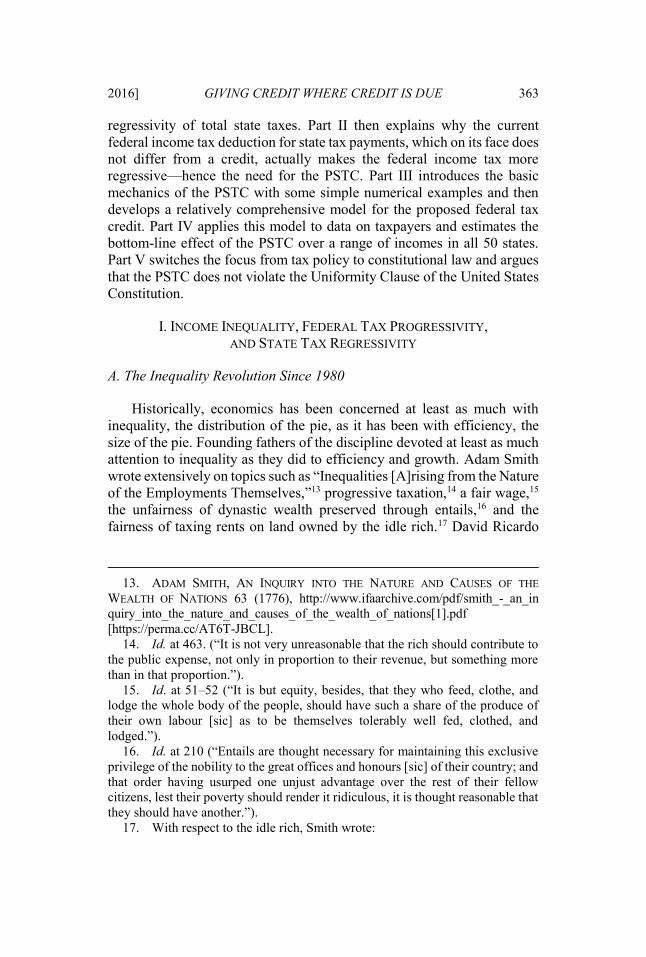
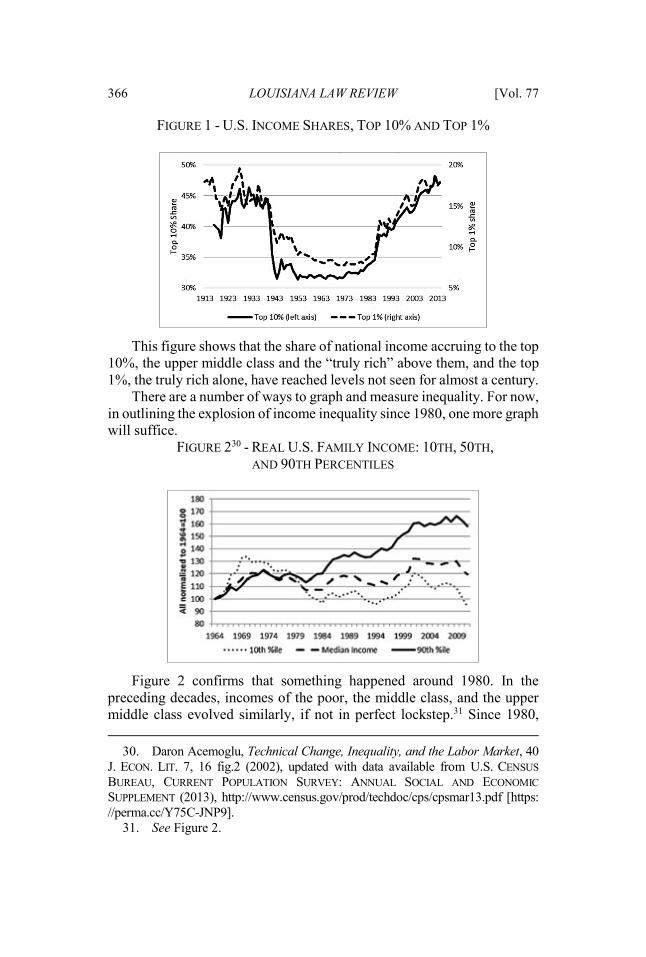
FIGURE 1 - U.S. INCOME SHARES, TOP 10% AND TOP 1%
This figure shows that the share of national income accruing to the top 10%, the upper middle class and the “truly rich” above them, and the top 1%, the truly rich alone, have reached levels not seen for almost a century.
There are a number of ways to graph and measure inequality. For now, in outlining the explosion of income inequality since 1980, one more graph will suffice.
FIGURE 230 - REAL U.S. FAMILY INCOME: 10TH, 50TH, AND 90TH PERCENTILES
Figure 2 confirms that something happened around 1980. In the preceding decades, incomes of the poor, the middle class, and the upper middle class evolved similarly, if not in perfect lockstep.31 Since 1980, 30. Daron Acemoglu, Technical Change, Inequality, and the Labor Market, 40 J. ECON. LIT. 7, 16 fig.2 (2002), updated with data available from U.S. CENSUS BUREAU, CURRENT POPULATION SURVEY: ANNUAL SOCIAL AND ECONOMIC SUPPLEMENT (2013), http://www.census.gov/prod/techdoc/cps/cpsmar13.pdf [https: //perma.cc/Y75C-JNP9]. 31. See Figure 2.
2016] GIVING CREDIT WHERE CREDIT IS DUE 367
however, the fortunes of the classes have diverged: poor and middle class households have experienced little if any income growth while wealthier Americans have enjoyed robust and consistent increases.32
The forces driving inequality vary across the income distribution. The stagnation in lower and middle incomes and the simultaneous rise in upper middle class incomes seems driven by what economists have labeled “skills-based technical change” (“SBTC”).33 Computers play a central role in this story. They have transformed the economy and the workplace; in particular, SBTC proponents argue that computers have markedly increased the productivity and hence the value of workers best able to use this new tool.34 Labor markets have responded as one would expect, by bidding up the price of those with the education and the intellectual aptitude to make the most productive use of computers.35 This response seems to explain why upper middle class incomes have fared so well since about 1980.
SBTC cannot explain the more spectacular income increases enjoyed by the top 1% over the same period. Increased productivity when working with computers cannot explain the stratospheric incomes now enjoyed by corporate executives, professional athletes, and entertainment stars. The leading explanation is “winner-take-all” (“WTA”) markets in which almost all of the gains flow to a very small group of top performers.36
Robert Frank’s example from the music industry nicely illustrates the WTA phenomenon. In 1900, Iowa had 1,300 opera houses.37 Iowans of
32. Id. 33. See generally David H. Autor, Lawrence F. Katz & Melissa S. Kearney, Trends in U.S. Wage Inequality: Revisiting the Revisionists, 90 REV. ECON. & STATISTICS 300, 300–02 (2008); CLAUDIA GOLDIN & LAWRENCE F. KATZ, THE RACE BETWEEN EDUCATION & TECHNOLOGY 287323 (2008). 34. See generally David Card & John E. DiNardo, Skill-Biased Technical Change and Rising Wage Inequality: Some Problems and Puzzles, 20 J. LAB. ECON. 733 (2002). 35. Id. 36. See ROBERT FRANK & PHILIP COOK, THE WINNER TAKE ALL SOCIETY (1996) (popularizing the term “winner take all”). Some seminal contributions to the literature on WTA markets are Thomas C. Schelling, Hockey Helmets, Concealed Weapons, and Daylight Savings: A Study of Binary Choices with Externalities, 17 J. CONFLICT RESOL. 381, 38182 (1973); Edward P. Lazear & Sherwin Rosen, Rank-Order Tournaments as Optimal Labor Contracts, 89 J. POL. ECON. 841, 84142 (1981); Sherwin Rosen, The Economics of Superstars, 71 AM. ECON. REV. 845, 84547 (1981); Sherwin Rosen, Prizes and Incentives in Elimination Tournaments, 76 AM. ECON. REV. 701, 701–02 (1986). 37. Interdisciplinary Program Series, The Wages of Stardom: Law and the Winner-Take-All Society: A Debate, 6 U. CHI. L. SCH. ROUNDTABLE 1, 3 (1999).
368 LOUISIANA LAW REVIEW [Vol. 77
that age could enjoy music only locally.38 Performers of only modest talent in the national or international pool of singers or musicians could earn a modest living if they were at or near the top of their local labor market.39 The record industry, television, computers, and the internet have changed everything. Today, Iowa no doubt has some local music venues, but surely nothing approaching 1,300. Iowans, along with New Yorkers, Oklahomans, Californians, Japanese, Russians, and just about all others can now enjoy the very best in any genre of entertainment. Jay Z doing hip-hop, Taylor Swift singing country or pop, Tom Cruise acting, Aaron Rodgers throwing touchdown passes—all are but a few remote control or mouse clicks away. These “winners” rake in the lion’s share of entertainment revenues, squeezing all but world-class talent out of these labor markets.40
The force of the two explanations for rising inequality, SBTC and WTA, seems unlikely to weaken any time soon. Computers and other innovations continue to enhance the value of smarts and education. Globalization continues apace, enabling tip-top talent to reach an even greater share of all Earth’s denizens. Thus, market forces cannot be expected to reduce the currently high levels of income inequality and indeed it seems likely that SBTC and WTA will continue to widen income gaps. One of the most obvious and effective tools for reducing market incomes is tax policy.
B. The Normative Case for Progressive Taxation
Section A presents stark facts suggesting that the U.S. faces a critical social policy question: should the government intervene to offset the effects of SBTC and WTA and reduce inequality from its historically high and still-rising levels? Is income inequality in fact a bad thing? Asked in this bald, unqualified fashion, the answer has to be “yes.” Given the option to choose government economic policies that yield very little income inequality, few would choose a different regime that yields much greater
38. Id. 39. Id. 40. WTA only partly explains the skyrocketing pay of top corporate executives. There is evidence that the market for top executives has become increasingly global. Xavier Gabaix & Augustin Landier, Why Has CEO Pay Increased So Much?, 123 Q. J. ECON. 49, 93–94 (2008). There is, however, other evidence suggesting that growing “agency problems”—too-cozy relationships between executives and the boards of directors that set their pay—explain a significant portion of rising compensation packages for corporate bigwigs. Lucian A. Bebchuk et al., The CEO Pay Slice, 102 J. FIN. ECON. 199, 199201 (2011).
2016] GIVING CREDIT WHERE CREDIT IS DUE 369
inequality with no concomitant increase in societal wealth. The following figure illustrates the idea behind this intuition.
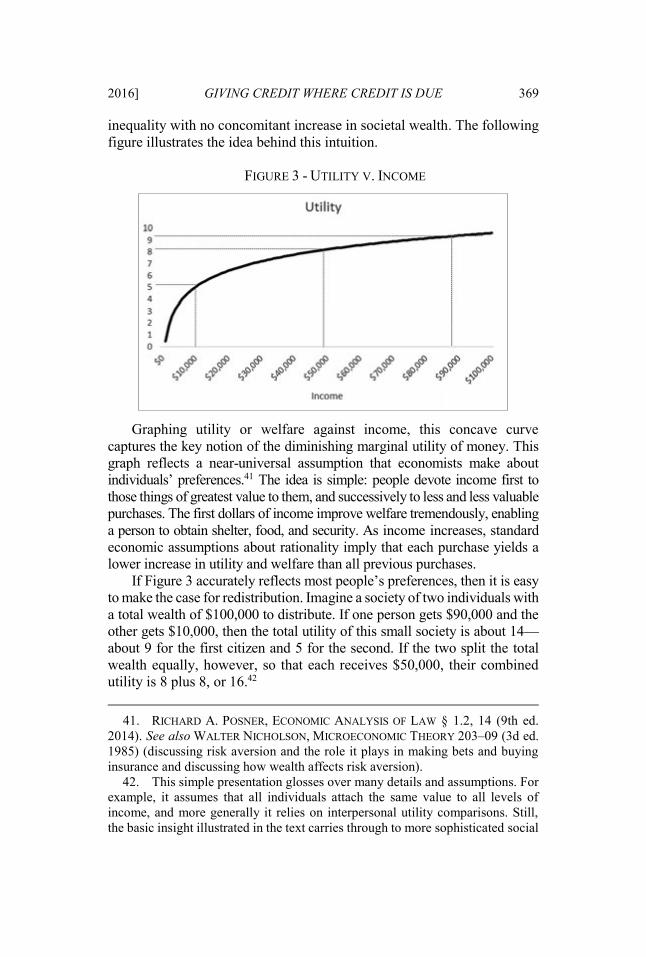
FIGURE 3 - UTILITY V. INCOME
Graphing utility or welfare against income, this concave curve captures the key notion of the diminishing marginal utility of money. This graph reflects a near-universal assumption that economists make about individuals’ preferences.41 The idea is simple: people devote income first to those things of greatest value to them, and successively to less and less valuable purchases. The first dollars of income improve welfare tremendously, enabling a person to obtain shelter, food, and security. As income increases, standard economic assumptions about rationality imply that each purchase yields a lower increase in utility and welfare than all previous purchases.
If Figure 3 accurately reflects most people’s preferences, then it is easy to make the case for redistribution. Imagine a society of two individuals with a total wealth of $100,000 to distribute. If one person gets $90,000 and the other gets $10,000, then the total utility of this small society is about 14—about 9 for the first citizen and 5 for the second. If the two split the total wealth equally, however, so that each receives $50,000, their combined utility is 8 plus 8, or 16.42 41. RICHARD A. POSNER, ECONOMIC ANALYSIS OF LAW § 1.2, 14 (9th ed. 2014). See also WALTER NICHOLSON, MICROECONOMIC THEORY 203–09 (3d ed. 1985) (discussing risk aversion and the role it plays in making bets and buying insurance and discussing how wealth affects risk aversion). 42. This simple presentation glosses over many details and assumptions. For example, it assumes that all individuals attach the same value to all levels of income, and more generally it relies on interpersonal utility comparisons. Still, the basic insight illustrated in the text carries through to more sophisticated social
370 LOUISIANA LAW REVIEW [Vol. 77
This relationship between utility and income, then, is the fundamental economic logic behind redistribution. Transferring income so that there are fewer yachts and mansions but more simple sedans and modest homes yields a net increase in total social utility and welfare. This scenario, however, is a radically incomplete story. If taken to its logical extreme, this ideal calls for taxes and transfer payments that leave everyone in the economy with equal after-tax-and-transfer income. Such a system fundamentally undermines effort and risk-taking—the size of the equally shared pie will be very small indeed.43
Starting with the path-breaking work of Nobel Prize winner James Mirrlees, economists have developed relatively sophisticated models to find the efficient trade-off between the benefits and the costs of redistributionary taxation.44 As one might suspect, the optimal tax structure depends on assumptions about the proper weight to place on relative equality and on the disincentive effect of income taxes at different levels of income.45 The former is entirely a value judgment; the latter is in theory determinable by empirical work, but in practice the range of estimates is quite wide. Thus, there is no consensus regarding the calculation of optimal tax rate structures. That said, a significant body of work suggests that a flat tax rate with a lump-sum transfer payment—a “demogrant”—of equal size to all taxpayers may closely approximate the tax system that best balances the tension between fairness and productivity.46
Accounting for the incentive effects of taxes and transfers weakens the “pure” case for redistribution embodied in Figure 3. Focusing only on income before and after taxes and transfers, however, is far too narrow a perspective. Examining a wider array of the deleterious effects of income inequality substantially buttresses the case for a more progressive tax system.
A burgeoning literature, largely from epidemiologists, argues that all citizens—be they poor, middle income, or rich—in regions and nations with higher income inequality experience poorer health outcomes than
welfare function models. See generally ROBIN W. BROADWAY & NEIL BRUCE, WELFARE ECONOMICS 137–94 (1991). 43. See generally RICHARD A. MUSGRAVE & PEGGY B. MUSGRAVE, PUBLIC FINANCE IN THEORY AND PRACTICE (5th ed. 1989). 44. See generally James A. Mirrlees, An Exploration in the Theory of Optimal Income Taxation, 38 REV. ECON. STUD. 175, 207–08 (1971); Nicholas Stern, On the Specification of Models of Optimum Taxation, 6 J. PUB. ECON. 123 (1976); Emmanuel Saez, Using Elasticities to Derive Optimal Income Tax Rates, 69 REV. ECON STUD. 205 (2001). 45. Mirrlees, supra note 44. 46. See id.
2016] GIVING CREDIT WHERE CREDIT IS DUE 371
citizens from similar regions or nations that exhibit less inequality.47 This hypothesis—the “relative income” hypothesis—is controversial, and a number of studies by economists have cast doubt upon it.48 If, however, there is any truth to this insight, the wealthy would have an affirmative reason to support the redistribution of some of their income to the less fortunate.
Even more disturbing than society-wide adverse health outcomes, increasing income inequality is stifling intergenerational economic mobility. Relatively wealthy parents are investing ever-growing sums to give their children a competitive advantage in school and in launching their careers; moreover, the gap between their outlays and what the middle class can afford has grown dramatically. In the early 1970s, parents in the top decile of incomes spent slightly more than two times what parents at the median spent on enriching their children’s educations and experiences; by 2007, they were spending four times as much.49 In our information age, education is the key to economic success, at least for those without winner-take-all talents that yield truly spectacular incomes.50 Recall that SBTC increasingly tilts income in favor of those best educated to use the wondrous new tools that technology keeps generating.51 The growing gap in expenditures on children by income level is projecting today’s inequality into future generations.
Thomas Piketty, in a recent book that has made a great impact on both sides of the Atlantic, raises another major concern with growing income inequality. Fundamental economic forces have been favoring returns to wealth, such as interest, dividends, and capital gains, over returns to labor, such as wages and salaries.52 He posits that those earning large incomes today and consequently accumulating great wealth will enjoy investment incomes that will grow at a faster rate than the labor incomes of the great
47. For an accessible recent summary of this hypothesis, see RICHARD WILKINSON & KATE PICKETT, THE SPIRIT LEVEL: WHY GREATER EQUALITY MAKES SOCIETIES STRONGER 1–12 (2009). See also S.V. Subramanian & Ichiro Kawachi, The Association Between State Income Inequality & Worse Health is not Confounded by Race, 32 INT’L J. EPIDEMIOLOGY 1022, 102228 (2003). 48. Angus Deaton, Health, Inequality, and Economic Development, 41 J. ECON LIT. 113, 115–16 (2003). 49. Sabino Kornitch & Frank Furstenberg, Investing in Children: Changes in Parental Spending on Children, 1972-2007, 50 DEMOGRAPHY 1, 13 tbl.2 (2012). 50. Employment Projections, BUREAU OF LAB. STAT., http://www.bls.gov/emp /ep_chart_001.htm [https://perma.cc/E5BD-RFFM] (last updated Mar. 15, 2016). 51. See supra Part I.A. 52. PIKETTY, supra note 3, at 198 fig.6.5.
372 LOUISIANA LAW REVIEW [Vol. 77
majority who lack significant wealth.53 This scenario is a prescription for overweening political power by a small circle of ever-wealthier families able to shape the law to protect their privileged positions. When combined with the rapid fading of the “rule against perpetuities”54 and the continued assault on the estate tax,55 America faces the possibility of dynastic wealth not seen for centuries.
There is widespread agreement among economists and tax scholars that income and perhaps wealth56 taxation and transfer policies are the best tools to reduce inequality.57 Income taxation reaches all citizens and precisely targets the source of inequality—unequal incomes. Other policy tools used to remedy inequality are much less suited to the task. Private law, such as contract, tort, and property, reaches a relatively small portion of the population in any given year, and shaping rules to redistribute income in these domains raises incentive concerns likely more costly than the modest disincentives created by the income tax.58 Minimum wage legislation and labor laws might help bolster lower and middle incomes to
53. Id. 54. As of 2012, almost half of the states in the U.S. had abolished the rule against perpetuities. William C. Spaulding, Rule Against Perpetuities: Modern Trend, THIS MATTER (Feb. 27, 2015), http://thismatter.com/money/wills-estates-trusts/rule-against-perpetuities-modern-trend.htm [https://perma.cc/J5PJ-5EZT]. 55. See, e.g., PUB. CITIZEN’S CONG. WATCH, SPENDING MILLIONS TO SAVE BILLIONS, THE CAMPAIGN OF THE SUPER WEALTHY TO KILL THE ESTATE TAX (2006), https://www.citizen.org/documents/EstateTaxFinal.pdf [https://perma.cc/4UVQ-HQ 8H]. 56. PIKETTY, supra note 3, at 447–67. 57. Walter J. Blum & Harry Kalven, Jr., The Uneasy Case for Progressive Taxation, 19 U. CHI. L. REV. 417, 417–19 (1952); Louis Kaplow & Steven Shavell, Why the Legal System is Less Efficient than the Income Tax in Redistributing Income, 23 J. LEGAL STUD. 667 (1994); Borys Grochulski, Distortionary Taxation for Efficient Redistribution, 95 ECON. Q. 235 (2009). 58. Kaplow & Shavell, supra note 57, at 667–69. For a response and subsequent rebuttals, see Chris Sanchirico, Taxes versus Legal Rules as Instruments for Equity: A More Equitable View, 29 J. LEGAL STUD. 797, 797–803 (2000); Louis Kaplow & Steven M. Shavell, Should Legal Rules Favor the Poor? Clarifying the Role of Legal Rules and the Income Tax in Redistributing Income, 29 J. LEGAL STUD. 821, 821–26 (2000); Chris Sanchirico, Deconstructing the New Efficiency Rationale, 86 CORNELL L. REV. 1003, 1069–70 (2001). Despite continual hue and cry to the contrary, longitudinal international data shows that there is essentially no evidence that higher marginal income tax rates have any adverse effect on economic growth. See, e.g., Thomas Piketty et al., Optimal Taxation of Top Labor Incomes: A Tale of Three Elasticities, 6 AM. ECON. J.: ECON. POL’Y 230, 256 fig.4A (2014).
2016] GIVING CREDIT WHERE CREDIT IS DUE 373
some extent, but they do nothing—at least not directly—to slow the explosion of income and wealth in the top 1% or 10%.
Reducing inequality in any serious way requires progressive income and wealth taxation. Progressive means that average tax rates—or effective tax rates (“ETRs”)—increase with income, and therefore the more a person makes, the higher the percent of income the person pays in taxes.59 Progressive taxation can redistribute income and reduce inequality without any transfer payments from rich to poor by imposing the lion’s share of the cost of public goods on those with the greatest capacity to pay.
C. Federal Tax Progressivity
This Article concentrates on the tax side of the redistribution toolkit. Before laying out the PSTC schema, it is helpful to tell a tale of contrasting tax regimes: the progressive federal system and the regressive state tax systems. Although there are many unfortunate regressive features of the federal income tax system,60 the rate structure has been progressive since the inception of the modern income tax in 1913.61 The degree of progressivity in federal income tax rates has varied widely over time.62 This progression is illustrated in Figure 4.
59. Progressive Tax in GRAHAM BANNOCK, R.E. BAXTER & EVAN DAVIS, THE PENGUIN DICTIONARY OF ECONOMICS (2003) (defining “progressive tax” as “[a] tax that takes an increasing proportion of income as income rises”). 60. Two examples: (1) capital gains on wealth are taxed at a lower rate than ordinary labor income despite the fact that wealth is distributed even more unevenly than income, and (2) corporations with significant profits are able to avoid income taxes altogether by using creative accounting and sham transactions. Stephen Moore, Capital Gains Taxes, in CONCISE ENCYCLOPEDIA OF ECONOMICS (David R. Henderson ed., 2d ed. 2008), http://www.econlib.org/library/Enc/CapitalGainsTaxes .html [https://perma.cc/47D8-L3BX]; ROBERT S. MCINTYRE ET AL., CITIZENS FOR TAX JUSTICE & INST. ON TAXATION AND ECON. POLICY, CORPORATE TAXPAYERS & CORPORATE TAX DODGERS 2008-2010, at 1–9 (2011). 61. See FEDERAL INDIVIDUAL INCOME TAX RATES HISTORY, supra note 5, at 1–68. In 1913, the marginal rate structure started at 1% for income under $20,000 and topped out at 7% for incomes over $500,000. U.S. Federal Individual Income Tax Rates History, 1862-2013, TAX FOUND. (Oct. 17, 2013), http://taxfoundation.org/arti cle/us-federal-individual-income-tax-rates-history-1913-2013-nominal-and-inflation -adjusted-brackets [https://perma.cc/F9H7-5KUV]. 62. Id.

374 LOUISIANA LAW REVIEW [Vol. 77
FIGURE 463 - U.S. TOP MARGINAL TAX RATES ON ORDINARY INCOME
Using the top marginal rate as an approximation of the progressivity
of the entire tax structure, progressivity peaked during and after World War II, with a top marginal rate of just over 90%. It began to decline with President Kennedy’s “Keynesian” tax cuts in the early 1960s; the fall in top marginal rates accelerated in the mid-1970s and has varied since then. As of 2014, the top marginal rate is 39.6%, less than half of its peak value. Still, given deductions and exemptions, federal income taxation retains a significant level of progressivity.64
Federal and state income taxes invariably define tax rates in terms of such marginal rates.65 To understand the meaning of a marginal tax rate, consider the following table of such rates for the U.S. in 2014.
63. Id. 64. CITIZENS FOR TAX JUSTICE, TOP FEDERAL INCOME TAX RATES SINCE 1913 (2011), http://www.ctj.org/pdf/regcg.pdf [https://perma.cc/R4GY-8T5N]. Note that these rates include some small substantive adjustments to the “official” rates listed in the statutes. 65. Federal marginal tax rates appear at 26 U.S.C. § 1 (2012) (“Taxes imposed”). For an example of marginal state income tax rates, see VA. CODE ANN. § 58.1-320 (West 2016).
2016] GIVING CREDIT WHERE CREDIT IS DUE 375
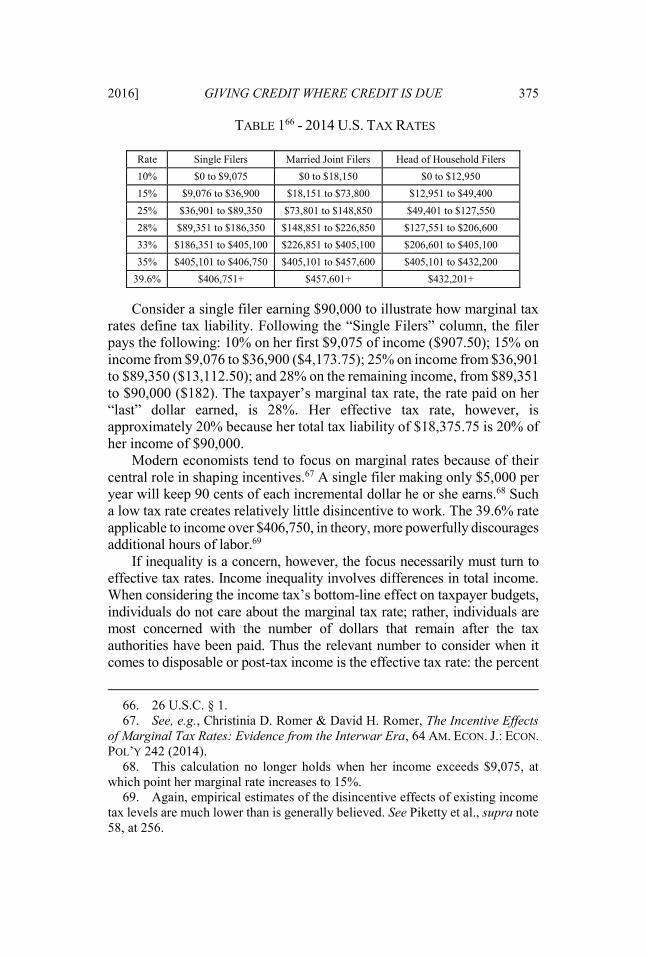
TABLE 166 - 2014 U.S. TAX RATES
Rate Single Filers Married Joint Filers Head of Household Filers 10% $0 to $9,075 $0 to $18,150 $0 to $12,950 15% $9,076 to $36,900 $18,151 to $73,800 $12,951 to $49,400 25% $36,901 to $89,350 $73,801 to $148,850 $49,401 to $127,550 28% $89,351 to $186,350 $148,851 to $226,850 $127,551 to $206,600 33% $186,351 to $405,100 $226,851 to $405,100 $206,601 to $405,100 35% $405,101 to $406,750 $405,101 to $457,600 $405,101 to $432,200
39.6% $406,751+ $457,601+ $432,201+
Consider a single filer earning $90,000 to illustrate how marginal tax
rates define tax liability. Following the “Single Filers” column, the filer pays the following: 10% on her first $9,075 of income ($907.50); 15% on income from $9,076 to $36,900 ($4,173.75); 25% on income from $36,901 to $89,350 ($13,112.50); and 28% on the remaining income, from $89,351 to $90,000 ($182). The taxpayer’s marginal tax rate, the rate paid on her “last” dollar earned, is 28%. Her effective tax rate, however, is approximately 20% because her total tax liability of $18,375.75 is 20% of her income of $90,000.
Modern economists tend to focus on marginal rates because of their central role in shaping incentives.67 A single filer making only $5,000 per year will keep 90 cents of each incremental dollar he or she earns.68 Such a low tax rate creates relatively little disincentive to work. The 39.6% rate applicable to income over $406,750, in theory, more powerfully discourages additional hours of labor.69
If inequality is a concern, however, the focus necessarily must turn to effective tax rates. Income inequality involves differences in total income. When considering the income tax’s bottom-line effect on taxpayer budgets, individuals do not care about the marginal tax rate; rather, individuals are most concerned with the number of dollars that remain after the tax authorities have been paid. Thus the relevant number to consider when it comes to disposable or post-tax income is the effective tax rate: the percent
66. 26 U.S.C. § 1. 67. See, e.g., Christinia D. Romer & David H. Romer, The Incentive Effects of Marginal Tax Rates: Evidence from the Interwar Era, 64 AM. ECON. J.: ECON. POL’Y 242 (2014). 68. This calculation no longer holds when her income exceeds $9,075, at which point her marginal rate increases to 15%. 69. Again, empirical estimates of the disincentive effects of existing income tax levels are much lower than is generally believed. See Piketty et al., supra note 58, at 256.
376 LOUISIANA LAW REVIEW [Vol. 77
of gross income paid to the government to satisfy tax liabilities. In light of this notion, this Article will examine effective tax rates instead of marginal tax rates. Specifically, this Article chooses to use effective tax rates because they more directly capture the fairness considerations that motivate progressive taxation.
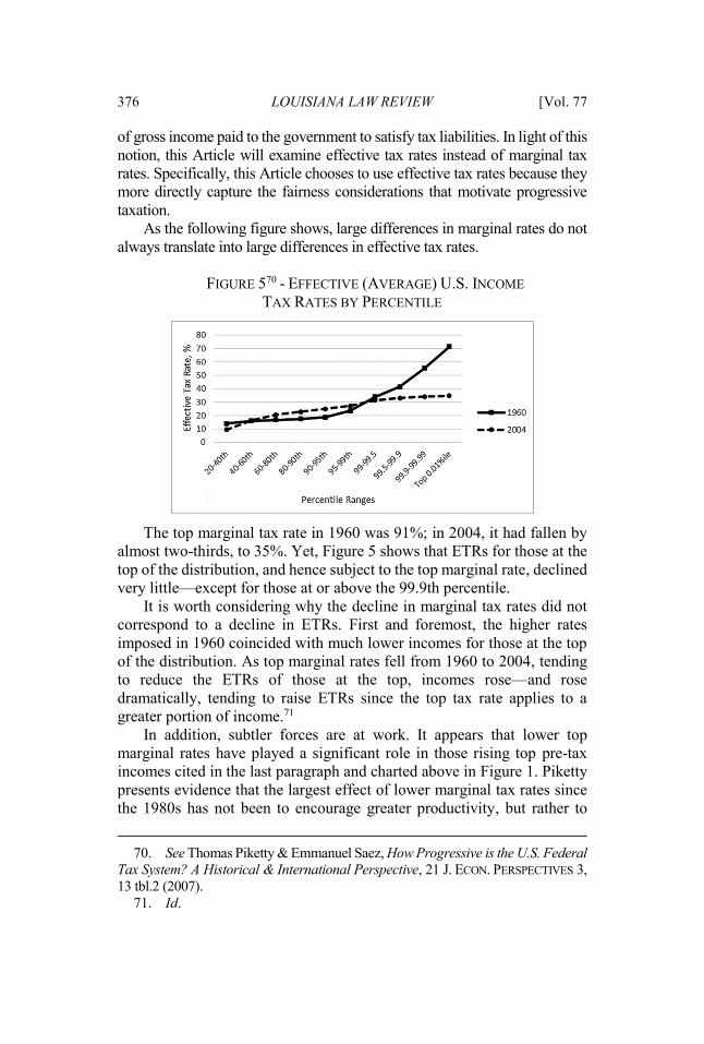
As the following figure shows, large differences in marginal rates do not always translate into large differences in effective tax rates.
FIGURE 570 - EFFECTIVE (AVERAGE) U.S. INCOME
TAX RATES BY PERCENTILE
The top marginal tax rate in 1960 was 91%; in 2004, it had fallen by almost two-thirds, to 35%. Yet, Figure 5 shows that ETRs for those at the top of the distribution, and hence subject to the top marginal rate, declined very little—except for those at or above the 99.9th percentile.
It is worth considering why the decline in marginal tax rates did not correspond to a decline in ETRs. First and foremost, the higher rates imposed in 1960 coincided with much lower incomes for those at the top of the distribution. As top marginal rates fell from 1960 to 2004, tending to reduce the ETRs of those at the top, incomes rose—and rose dramatically, tending to raise ETRs since the top tax rate applies to a greater portion of income.71
In addition, subtler forces are at work. It appears that lower top marginal rates have played a significant role in those rising top pre-tax incomes cited in the last paragraph and charted above in Figure 1. Piketty presents evidence that the largest effect of lower marginal tax rates since the 1980s has not been to encourage greater productivity, but rather to
70. See Thomas Piketty & Emmanuel Saez, How Progressive is the U.S. Federal Tax System? A Historical & International Perspective, 21 J. ECON. PERSPECTIVES 3, 13 tbl.2 (2007). 71. Id.
2016] GIVING CREDIT WHERE CREDIT IS DUE 377
create incentives for top earners, especially corporate executives, to raise their compensation.72 Lower top marginal tax rates create clear incentives for managers to exploit agency problems and informational advantages when they bargain for compensation.73 Thus although high marginal rates may not increase average tax rates, they may serve the salutary purpose of substantially muting the incentives of executives to work their boards of directors for exorbitant pay and perks.
Finally, Figure 5 shows that effective federal tax rates at the bottom of the income distribution have become lower, increasing progressivity. The earned income tax credit and higher exemption levels explain most of this reduction in the federal tax burden imposed on the poorest households.74 Combining this tilt in favor of those at the bottom with the previous discussion of rates at the top, the current federal income tax earns relatively high marks for progressivity—effective rates increase steadily and noticeably with income.
D. State Tax Regressivity
The states’ individual tax regimes, in stark contrast, earn dreadful marks for progressivity. In every state, the combined effect of all taxes is actually regressive. When looking at federal taxation, this Article considers only the income tax, as it accounts for an overwhelming share of revenue.75 Almost every state, however, imposes other taxes that account for a significant share of total state revenue, often a majority. Indeed, some states have no income
72. Piketty et al., supra note 58, at 251. 73. After all, if a manager’s marginal tax rate falls from 50% to 25%, she will take home 75 instead of 50 cents of each incremental dollar for which she successfully bargains. Any informational advantages that she has over the board of directors that enable her to bargain for greater compensation rise in value by one-third (from 50 cents per marginal dollar to 75 cents), and this greater payoff gives her strong incentives to exploit all such informational asymmetries. 74. See Nada Eissa & Hilary Hoynes, Redistribution and Tax Expenditures: The Earned Income Tax Credit, 64 NAT. TAX J. 689, 689–91 (2011). 75. Social Security and Medicare payroll taxes are excluded. Social Security payments in theory are contributions returned as retirement benefits later in life, though in substance it is not clear that this result is the case. SOC. SEC. ADMIN., SOCIAL SECURITY: UNDERSTANDING THE BENEFITS 45 (2015), http://www.ssa.gov/pubs/EN -05-10024.pdf [https://perma.cc/7D6E-99E7]. Additionally, Medicare taxes can be thought of as payments by workers to fund health care on retirement. Katherine Baicker & Michael E. Chernew, The Economics of Financing Medicare, 365 NEW ENGLAND J. MED. 1056, 1056–59 (2011), http://www.nejm.org/doi/full/10.1056 /NEJMp1107671#t=article [https://perma.cc/S836-Y5YF].
378 LOUISIANA LAW REVIEW [Vol. 77
tax.76 Thus, to assess accurately the progressivity or regressivity of state taxation overall, one must consider the combined effect of multiple taxes that contribute significant amounts to states’ revenue. The effective rates of sales and property taxes must be estimated from taxpayers’ incomes and consumption patterns.
The basic reason that state taxes are so regressive is simple: sales taxes are a major source of revenue in most states.77 Sales taxes apply only to consumption, and the higher a household’s income, the smaller the fraction of that income the household spends on consumption.78 Although state income taxes provide some progressivity to counter the regressive nature of state taxes, it is not much. The marginal rate structures tend to be only mildly progressive and have many deductions and exemptions favorable to higher income households.79 The real property tax is the murkiest component of state taxation, as there is significant uncertainty about whether tenants pay higher rent because of property taxes or whether their landlords must absorb this cost.80 Therefore, there is considerable uncertainty about the incidence of the property tax. The bottom line, however, is that overall effective tax rates vary inversely with income in every single state—and thus rates are regressive. A comprehensive survey of the tax system of all 50 states provides evidence of this conclusion:
76. Alaska, Florida, Nevada, South Dakota, Texas, Washington, and Wyoming have no state income taxes. Liz Malm & Ellen Kant, The Sources of State and Local Tax Revenues, TAX FOUND. (Jan. 28, 2013), http://taxfoundation.org/article/sources-state-and-local-tax-revenues [https://perma.cc/ZBU5-JNBV]. In addition, Tennessee and New Hampshire have almost no income tax; however, both states impose a small tax (5% or 6%) on interest and dividend income. TENN. CODE ANN. § 67-2-102 (West 2016); N.H. REV. STAT. ANN. § 77:4 (2016); see also Frequently Asked Questions – Interest & Dividend Tax, N.H. DEP’T OF REVENUE ADMIN, http://revenue.nh.gov/faq /interest-dividend.htm [https://perma.cc/CU8Z-C7KQ] (last visited Oct. 18, 2016). Admittedly, these small taxes are highly progressive as wealthy households’ share of interest and dividend income is even higher than their share of labor income. 77. State Sales Tax Rates, SALES TAX INST., http://www.salestaxinstitute.com/re sources/rates [https://perma.cc/34DK-WDNC] (last updated Sept. 1, 2016) (rates); State Government Tax Collections: 2015, AM. FACT FINDER (Sept. 23, 2016), http://factfinder.census.gov/faces/tableservices/jsf/pages/productview.xhtml?src=bk mk [https://perma.cc/857M-P48A] (revenues). Only four states have no state or local sales tax: Delaware, Montana, New Hampshire, and Oregon. Alaska has no state sales tax but permits localities to impose one. Id. 78. Regressive Tax, INVESTOPEDIA, http://www.investopedia.com/terms/r /regressivetax.asp [https://perma.cc/28CP-UEVJ] (last visited Oct. 18, 2016) (explaining why sales taxes are regressive). 79. DAVIS ET AL., supra note 7, at 8–12. 80. See infra text accompanying notes 93–98.
2016] GIVING CREDIT WHERE CREDIT IS DUE 379
Virtually every state’s tax system is fundamentally unfair, taking a much greater share of income from low- and middle-income families than from wealthy families . . . . Combining all state and local income, property, sales and excise taxes that Americans pay, the nationwide average effective state and local tax rates by income group are 10.9 percent for the poorest 20 percent of individuals and families, 9.4 percent for the middle 20 percent and 5.4 percent for the top 1 percent.81
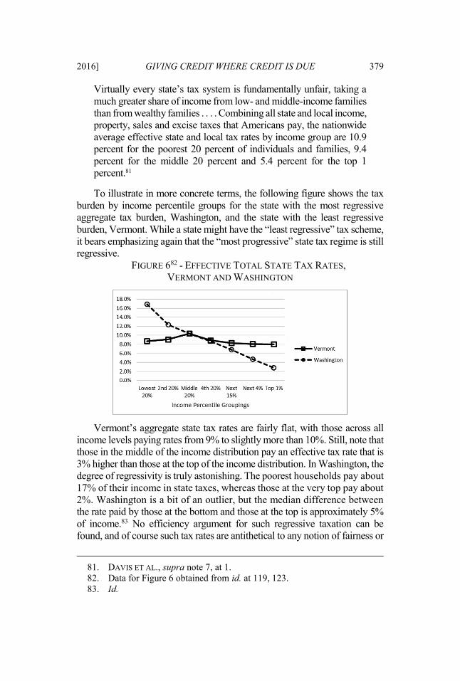
To illustrate in more concrete terms, the following figure shows the tax burden by income percentile groups for the state with the most regressive aggregate tax burden, Washington, and the state with the least regressive burden, Vermont. While a state might have the “least regressive” tax scheme, it bears emphasizing again that the “most progressive” state tax regime is still regressive.
FIGURE 682 - EFFECTIVE TOTAL STATE TAX RATES, VERMONT AND WASHINGTON
Vermont’s aggregate state tax rates are fairly flat, with those across all income levels paying rates from 9% to slightly more than 10%. Still, note that those in the middle of the income distribution pay an effective tax rate that is 3% higher than those at the top of the income distribution. In Washington, the degree of regressivity is truly astonishing. The poorest households pay about 17% of their income in state taxes, whereas those at the very top pay about 2%. Washington is a bit of an outlier, but the median difference between the rate paid by those at the bottom and those at the top is approximately 5% of income.83 No efficiency argument for such regressive taxation can be found, and of course such tax rates are antithetical to any notion of fairness or
81. DAVIS ET AL., supra note 7, at 1. 82. Data for Figure 6 obtained from id. at 119, 123. 83. Id.

380 LOUISIANA LAW REVIEW [Vol. 77
equity. These rates are reminiscent of the allocation of tax burdens in feudal societies.84
Regressive state taxation has inevitable effects on lower income households. Consider the state of Washington as an example. A family with an annual income of $20,000 pays 17% of that income to the state, or about $3,400. If Washington adopted even a flat tax system, each household would have to pay about 7% of its income in state taxes.85 For a family with an income of $20,000, that comes to $1,400—$2,000 less than under current Washington law. A couple with one child earning $20,000 a year falls below the poverty line.86 An extra $2,000 would make a huge difference to such a family, funding necessities like food, safe housing, and the purchase of a car. In the abstract, regressive taxation sounds like another obscure and complex policy issue. In reality, regressive state taxation unfairly deprives poor and middle class families of basic commodities and opportunities.
Consistent with many other major policy shifts over the last few decades, state taxation has become more regressive. There is no readily available data before 1995, but over the last two decades the following figure shows the trend.
FIGURE 787 - AVERAGE STATE TAX RATE BY INCOME PERCENTILES
84. Eric Kades, The New Feudalism (unpublished manuscript) (on file with author). See also MEHRDAD VAHABI, THE POLITICAL ECONOMY OF PREDATION: MANHUNTING AND THE ECONOMICS OF ESCAPE 267 (2015) (“The tax system in the feudal age was highly regressive and put a heavy tax burden on peasants while allowing privileges and personal exemption to members of the upper classes.”) (internal quotation omitted) (citation omitted). 85. Based on author’s calculations using data appearing in Figure 6. 86. U.S. DEP’T OF HEALTH & HUMAN SVCS., 2015 POVERTY GUIDELINES 2 (2015), https://aspe.hhs.gov/2015-poverty-guidelines#threshholds [https://perma.cc /99M4-JBJR]. 87. MICHAEL P. ETTLINGER ET AL., CITIZENS FOR TAX JUSTICE & THE INST. ON TAXATION & ECON. POLICY, WHO PAYS? A DISTRIBUTIONAL ANALYSIS OF THE TAX SYSTEMS IN ALL 50 STATES 1 (1st ed. 1996); DAVIS ET AL., supra note 7, at 3.

2016] GIVING CREDIT WHERE CREDIT IS DUE 381
As Figure 7 illustrates, rates fell across the board, reflecting a slight
reduction in state taxes from 1995 to 2015. The bottom 20% actually fared better than most higher income groups, with a decline in their effective tax rate of 1.6%.88 The middle percentiles saw their total state tax rate fall by a modest 0.6% to 0.8%.89 Those in the top 1% of incomes, however, experienced a 2.5% decrease in their effective aggregated state tax rate,90 by far the largest decline of any group. Given that tax rates on these households did not noticeably increase, much of this decrease can only be explained by soaring incomes at the top of the distribution. These taxpayers save high proportions of incremental earnings, and thus this income escapes sales and other excise taxes.91 Still, even if this outsized state tax cut is not the result of express legislation and regulation favoring wealthy households since 1996, the fact that state political actors have apparently felt no need to restructure their tax regimes to reduce regressivity during an era of sharply rising inequality is itself an implicit policy choice to increase rather than decrease inequality in relative tax burdens.
As this analysis suggests, the centerpiece of regressive state taxation is the sales tax. This consumption tax ends up being significantly regressive because the poor consume essentially all of their income, and thus all of their income is taxed, while the portion of income saved by wealthier households is either not taxed at all, if a state has no income tax, or is taxed at a relatively low rate.92 Averaged over all 50 states, “[p]oor families pay almost eight times more of their incomes in [sales] taxes than the best-off families,93 and middle-income families pay more than five times the rate of the wealthy.”94 In Washington, for example, the poorest 20% of households pay 12.6% of their income to sales taxes, while the wealthiest 1% pay a rate of only 1.6%.95 Thus the appearance of sales taxes as “flat” taxes is deceptive because in practice, the taxes are extremely regressive.
Some states fail to take even the simplest measures to make their sales tax less regressive. For instance, one simple way to avoid regressive is to 88. Id. 89. Id. 90. Id. 91. Karen E. Dynan, Jonathan Skinner, & Stephen P. Zeldes, Do the Rich Save More?, 112 J. POL. ECON. 397 (2004) (finding savings rate increases with income). 92. Id. 93. Poor families pay approximately 7% while best-off pay 0.9%. DAVIS ET AL., supra note 7, at 6. 94. Id. 95. Id. at 123.

382 LOUISIANA LAW REVIEW [Vol. 77
exempt necessities from the sales tax. The poor by definition spend a greater share of their incomes on necessities, and so taxing such goods is inherently regressive. The most obvious example is food. “Taxing food is a particularly regressive strategy because poor families spend most of their income on groceries and other necessities.”96 Expanding on the theme, sales taxes on gasoline, beer, and cigarettes fall disproportionately, in terms of ETRs, on lower income households.97 In keeping with trending inequality, Kansas and South Dakota recently eliminated tax credits and refunds for food purchases, tilting their tax systems further in the direction of regressivity.98
Property taxes, although usually assessed by localities rather than states, are likely regressive. Under some assumptions, however, property taxes might be mildly progressive. To start, in virtually all localities the real property tax is assessed at a flat rate, called the “millage.”99 For reasons that are not entirely clear, progressive real property tax rates are extremely rare in the U.S.,100 despite the fact that some of the most prominent Founding Fathers ardently advocated such regimes. Thomas Jefferson lauded a progressive property tax, stating that “a means of silently lessening the inequality of property is to exempt all from taxation below a certain point, and to tax the higher portions of property in geometrical progression as they rise.”101 Despite residing on the other side
96. Id. at 12. 97. Id. at 13. 98. KAN. LEGISLATIVE RESEARCH DEP’T, TAX REDUCTION AND REFORM; SENATE SUB. FOR HB 2117, at 1 (2012) http://kslegislature.org/li_2012/b2011_12 /measures/documents/summary_hb_2117_2012.pdf [https://perma.cc/56TX-6KR9]; Joy Smolnisky, Should SD Repeal the Grocery Tax with a Revenue Neutral Sales Tax Increase?, S.D. BUDGET & POL’Y INST. (Feb. 5, 2013), http://www.sdbpi.org/should-sd-repeal-the-grocery-sales-tax-with-a-revenue-neutral-sales-tax-increase [https://per a.cc/C3VC-NJQ7]. The law was enacted and codified at S.D. CODIFIED LAWS § 10-45-2 (2016). 99. Millage Rate, INVESTOPEDIA, http://www.investopedia.com/terms/m/mil agerate.asp [https://perma.cc/59PC-222E] (last visited Oct. 21, 2016) (explaining why sales taxes are regressive). 100. See, e.g., VIRGINIA DEP’T OF TAXATION, LOCAL TAX RATES 2014, http://www.tax.virginia.gov/sites/tax.virginia.gov/files/Local%20Tax%20Rates%20 TY%202014_March%2024th%202016.pdf [https://perma.cc/GX68-6RDX] (flat tax on real estate by locality); Benchmarking New York: Property Taxes in New York Communities, EMPIRE CTR., http://www.empirecenter.org/wp-content/uploads/2016 /06/Benchmarking2014 rates.pdf [https://perma.cc/AG8W-63E6] (last visited Nov. 11, 2016) (same). 101. Letter from Thomas Jefferson to James Madison, in 3 THE PAPERS OF THOMAS JEFFERSON 681, 682 (Julian P. Boyd ed., 1785) (1953).
2016] GIVING CREDIT WHERE CREDIT IS DUE 383
of the political spectrum, Alexander Hamilton agreed and proposed a property tax rate structure with rates starting at 20 cents per room for log cabins and rising to $1 per room for homes with more than six rooms.102 In 1791, Congress actually passed a different progressive property tax that imposed a rate of 0.2% for homes valued up to $1,000 and maxed out at 1% for homes worth $30,000 or more.103
Although a flat tax gives property taxation the appearance of straddling the line between progressive and regressive taxes, the pattern of asset ownership in America introduces a distinct regressive bias. If the share of families’ wealth in the form of houses did not vary with income, a flat property tax rate would translate into a truly flat property tax—the effective tax rate would not vary with household income. The premise in the previous sentence assuming no income-based differences in housing as a percentage of wealth, however, does not hold.
For average families, a home represents the lion’s share of their total wealth. At high income levels, however, homes are only a small share of total wealth. Because the property tax usually applies mainly to homes and exempts most other forms of wealth, the tax applies to most of the wealth of middle income families, and hits a smaller share of the wealth of high-income families.104
Just as flat sales taxes are regressive in practice because of the negative correlation between income and the percent of income spent on consumption, flat property taxes are presumptively regressive because they impact a form of wealth that declines as a percent of total wealth as income rises.
This presumption, however, may be rebuttable. Attempts to discern who exactly pays the property tax have proven extremely difficult. One important issue is the extent to which landlords, formally required to cut property tax checks to the government as owners, can pass along the increase to lessees in the form of higher rents. If, for example, landlords can raise rents to cover their entire property tax bill, then the tax in substance is paid for by renters even if landlords formally make the tax
102. GLENN W. FISHER, THE WORST TAX?: A HISTORY OF THE PROPERTY TAX IN AMERICA 40 (1996). 103. 1 HENRY CARTER ADAMS, TAXATION IN THE UNITED STATES, 1789-1816, at 5456 (Burt Franklin ed., 1970) (1884). Singapore recently enacted a progressive property tax to make home ownership more feasible for middle-income households. Jessica Cheam, Singapore Shifting to New Progressive Property Tax System, CHINA POST (Feb. 24, 2010), http://www.chinapost.com.tw/print/245733.htm [https://per ma.cc/X4AV-CCZ4]. 104. DAVIS ET AL., supra note 7, at 13.

384 LOUISIANA LAW REVIEW [Vol. 77
payment. The issue is critical to determining the regressivity or progressivity of the property tax because renting households on average have significantly lower income than landlords and spend a large portion of their income on rent.105 If renters bear the lion’s share of property taxes, the taxes will be markedly regressive.
Most agree that landlords can cover some portion, rather than all, of their property taxes with higher rent.106 To assess the tax’s regressivity or progressivity, however, it is important to know how much of the property tax falls on tenants. Unfortunately, assumptions rather than data drive results. Under one set of assumptions, “[p]roperty taxes . . . are usually somewhat regressive . . . poor homeowners and renters pay more of their incomes in property taxes than do any other income group—and the wealthiest taxpayers pay the least.”107 In support of this perspective, one study found that “apartment residents pay a property tax 39 percent higher than that of homeowners of the same long-run income.”108 Seemingly contradictory, another study found that tenants bear only 15% of property taxes.109 If we follow this estimate and assume that property taxes fall largely on owners, property taxes might be progressive enough to offset the considerable regressivity of state sales taxes.110
Unlike sales taxes and with greater certainty than property taxes, state income taxes generally have modestly progressive rates and serve as a counterweight to regressive sales taxes.111 States without income taxes,
105. Id. at 13–14. 106. See, e.g., George Zodrow, Who Pays the Property Tax?, 18 LAND LINES 14 (2006). The general proposition here is that only under unusual circumstances does the true incidence of a tax fall 100% on the buyer or the seller. Tax Incidence: How the Tax Burden is Shared between Buyers and Sellers, THIS MATTER, http://thismatter .com/economics/tax-incidence.htm [https://perma.cc/XPQ9-8NPU] (last visited Oct. 18, 2016) (“Only if either demand or supply was either completely elastic or inelastic will the tax burden fall entirely on either the buyer or the seller. Between these 2 extremes, tax incidence varies continuously from a perfectly inelastic supply or perfectly elastic demand, where the sellers assume the entire burden of the tax to the perfectly elastic supply or perfectly inelastic demand where the buyers bear the entire burden.”). 107. Zodrow, supra note 106, at 16. 108. Jack Goodman, Houses, Apartments, and Property Tax Incidence 16 (Harvard Univ. Joint Ctr. for Hous. Studies, Paper No. W05-2) (2005), http://www .jchs.harvard.edu/sites/jchs.harvard.edu/files/w05-2.pdf [https://perma.cc/95HL-H VJZ]. 109. Robert J. Carroll & John Yinger, Is the Property Tax a Benefit Tax? The Case of Rental Housing, 47 NAT. TAX J. 295, 310–11 (1994). 110. JOSEPH A. PECHMAN, WHO PAID THE TAXES: 1966-85?, at 29–34 (1985). 111. DAVIS ET AL., supra note 7, at 8–11.

2016] GIVING CREDIT WHERE CREDIT IS DUE 385
such as Washington, Florida, and Texas, tend to have the most regressive overall state tax burdens;112 “these states’ disproportionate reliance on sales and excise taxes make their taxes among the highest in the entire nation on low-income families.”113 In Washington, the bottom 20% pay an aggregate state tax rate of 16.9% of income, in Florida 12.9%, and in Texas 12.5%.114 Even in states with some progressivity in their income tax rates, the regressivity of sales taxes more than offsets the modest progressivity of these state income taxes.115
The final element of regressive state taxation involves a subtle interaction with the federal tax code—the ability to deduct state taxes from the measure of income used to compute federal tax liability.116 The taxpayer must elect to itemize deductions to take advantage of this deduction.117 Most low-income and many middle-income households, however, cannot use this deduction, as they often elect the standard deduction.118 Therefore, the deductibility of state tax payments hardly benefits those at the bottom or in the middle of the income distribution but significantly and increasingly benefits those at the top—which is essentially the definition of a regressive tax rule.
Reforming regressive state tax systems seems like a nearly impossible political task. The reform would involve taking on powerful interest groups in all 50 states and would require the introduction of, or a major overhaul to, multiple taxes in most states. To correct the regressive tax structure of even one state would be an impressive accomplishment; to fix ten states seems virtually impossible; and to undo the regressive tax systems in all 50 states seems patently impossible. Yet, correcting regressivity is precisely the promise of the PSTC.
112. Id. at 4. 113. Id. at 15. 114. Id. at 47, 115, 123. 115. Id. at 1. 116. 26 U.S.C. § 164 (2012). 117. Topic 501 - Should I Itemize?, INTERNAL REVENUE SERV. (Oct. 20, 2016), https://www.irs.gov/taxtopics/tc501.html [https://perma.cc/J6VL-BL4P]. 118. Kay Bell, Tax Loopholes That Mainly Benefit the Rich, BANKRATE, http://www.bankrate.com/finance/taxes/tax-loopholes-mainly-benefit-rich-1.aspx [https://perma.cc/HE8X-JE2V] (last visited Oct. 21, 2016) (noting that only a third of households file itemized deductions with their federal tax returns).
386 LOUISIANA LAW REVIEW [Vol. 77
II. DEDUCTIONS AND CREDITS, PROGRESSIVE OR REGRESSIVE, AND INTERACTIONS BETWEEN NATIONAL AND STATE TAXATION
The United States tax code has long permitted taxpayers to deduct state tax payments from income subject to the federal income tax.119 Although it might seem that the PSTC will have the same progressive impact as the current deductibility of state taxes, that is unequivocally false. Understanding this difference in effect depends upon understanding the difference between an income tax deduction and an income tax credit.
A deduction for state income taxes means that a taxpayer can deduct his or her state tax payments120 from pre-tax income, which lowers income for federal tax purposes and thus lowers the total federal income tax bill. A credit, on the other hand, applies after a taxpayer has calculated his or her tax bill.121 Thus a tax credit reduces tax liability dollar for dollar.
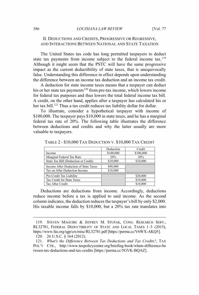
To illustrate, consider a hypothetical taxpayer with income of $100,000. The taxpayer pays $10,000 in state taxes, and he has a marginal federal tax rate of 20%. The following table illustrates the difference between deductions and credits and why the latter usually are more valuable to taxpayers.
TABLE 2 - $10,000 TAX DEDUCTION V. $10,000 TAX CREDIT
Deduction Credit Income $100,000 $100,000 Marginal Federal Tax Rate 20% 20% State Tax Bill (Deduction or Credit) $10,000 $10,000
Income After Deduction of State Taxes $90,000 Tax on After Deduction Income $18,000 Pre-Credit Tax Liability
$20,000
Tax Credit for State Taxes $10,000 Tax After Credit $10,000
Deductions are deductions from income. Accordingly, deductions reduce income before a tax is applied to said income. As the second column indicates, the deduction reduces the taxpayer’s bill by only $2,000. His taxable income falls by $10,000, but a 20% tax rate translates into
119. STEVEN MAGUIRE & JEFFREY M. STUPAK, CONG. RESEARCH SERV., RL32781, FEDERAL DEDUCTIBILITY OF STATE AND LOCAL TAXES 1–3 (2015), https://www.fas.org/sgp/crs/misc/RL32781.pdf [https://perma.cc/V6WX-AKQ5]. 120. 26 U.S.C. § 164 (2012). 121. What's the Difference Between Tax Deductions and Tax Credits?, TAX POL’Y CTR., http://www.taxpolicycenter.org/briefing-book/whats-difference-be tween-tax-deductions-and-tax-credits [https://perma.cc/5GVK-BQAZ].
2016] GIVING CREDIT WHERE CREDIT IS DUE 387
bottom-line savings of only 20% of $10,000, or $2,000. In contrast, a tax credit applies after total tax liability has been calculated. As the third column shows, the credit reduces the tax liability by the full $10,000. In this example, the credit is five times more valuable to the taxpayer than the deduction because the credit yields tax savings of $10,000, whereas the deduction yields savings of only $2,000.
As currently implemented, the federal deduction for state tax payments is surprisingly regressive, benefitting high-income taxpayers more than others. There are two reasons for this regression. First and foremost, deductions are valuable only to relatively high-income taxpayers; others are better off taking their standard deduction, which is a fixed amount that does not vary with state tax payments. Only one-third of all households itemize, and this group is “a population that consists primarily of high-income, high-wealth taxpayers.”122 Second, as suggested by the simple example above, the value of the state tax deduction, like all deductions, varies directly with marginal tax rates. If one’s marginal rate is 50%, a $100 deduction saves $50; but if the marginal rate is 10%, the deduction saves only $10.123 Given the progressive marginal rate structure of the federal income tax, along with the Earned Income Tax Credit available to lower income households, the ability to deduct state tax payments in practice benefits the wealthy much more than middle- and low-income taxpayers.124 Thus, the deduction for state and local taxes does an abysmal job of allocating the federal income tax burden so that it more closely aligns with ability to pay. Indeed, it amounts to a tax break for wealthier households that is of no value to their lower income counterparts.
A simple 100% federal tax credit for all taxpayers suffers from neither of these two regressive features. First, with an important caveat, credits are equally valuable to low- and high-income households. The caveat is that the credit must be one that a taxpayer may use even if applying the credit results
122. Kirk Stark, Fiscal Federalism & Tax Progressivity: Should the Federal Income Tax Encourage State & Local Redistribution?, 51 U.C.L.A. L. REV. 1389, 1394 (2004). 123. Id. at 1416 (“The value of any federal deduction is equal to the amount of the deduction multiplied by the taxpayer's marginal tax rate.”). 124. Congress has gyrated over the years on the deductibility of state sales taxes. They were deductible until 1986, but were not from then until 2004. Since 2004, Congress has reauthorized sales tax deduction every few years, but each time they have done so for a relative short horizon of one or two years. MAGUIRE & STUPAK, supra note 119, at 1–4. Permitting deduction of state income and property taxes while denying deduction of sales taxes of course biases federal tax incidence in favor of wealthy households that pay relatively high income and property rates but relatively low sales tax ETRs.
388 LOUISIANA LAW REVIEW [Vol. 77
in a negative tax due—such that the government writes the taxpayer a check instead of vice versa. Many, though not all, federal tax credits allow for this tax benefit.125 This caveat is important because most low-income taxpayers have zero or negative federal income tax liability before considering their state tax payments. For a credit to benefit these households, the credit for state tax payments must entitle taxpayers to a check from the U.S. Treasury. In contrast, it is difficult to construct a case in which deductions benefit poorer households. Deductions generally cannot exceed total income, and so they cannot give rise to a governmental obligation to make a “negative” tax payment.126
Second, unlike a deduction, the benefit of a credit in an environment of regressive state taxation is actually progressive. To illustrate, consider a state with a tax system that imposes a 20% burden on incomes below $50,000 and a 5% burden on higher incomes.127 Under a 100% federal income tax credit for state tax payments, taxpayers earning $10,000 would get a credit of $2,000—20% of their income. Taxpayers earning $100,000 would get a credit of $5,000—only 5% of their income. Indeed, the more regressive a state’s tax regime, the more progressive a federal credit for state taxes.
Although a credit for state tax payments would be free from the current deduction’s regressive drawbacks, both share problems. First and most obviously, neither is revenue neutral. Enacting either without offsetting tax increases would result in lower federal tax revenue. With a deduction or a credit that reduces federal revenue, a national government with a fixed need for revenue must tax elsewhere or borrow. How the federal government would reduce taxes elsewhere if it jettisoned the current regressive deduction for state tax payments is unknown. A natural baseline assumption is that the government would decrease income taxes across the board. This means that the federal income tax would tend to be more progressive without the state tax deduction. Less affluent households would enjoy an unadulterated tax cut, while the benefit of the general tax cut to wealthier households would be offset significantly by the elimination of the valuable state tax deduction.
125. See, e.g., 26 U.S.C. § 24 (2012), “Child Tax Credit” (partially refundable); id. § 25A, “American Opportunity Credit (partially refundable); id. § 25D, “Residential Energy Efficient Property Credit” (not refundable). 126. Limits on Itemized Deductions, INTERNAL REVENUE SERV., https://www .irs.gov/publications/p17/ch29.html [https://perma.cc/7GY6-2D6L] (last visited Oct. 18, 2016). 127. This example is not that unrealistic; it approximates the state tax regimes in the state of Washington and others with highly regressive reliance on sales taxation.
2016] GIVING CREDIT WHERE CREDIT IS DUE 389
Deductions and credits share another problem. Both create incentives for states and taxpayers to engage in perverse and wasteful behavior. They encourage states to “export” their aggregate tax liability to other states by choosing taxes that maximize the total deductions created for their citizens on their federal income tax returns. Given the fixed revenue need of the national government, less tax revenue from one state because of larger deductions or credits for state taxes means that more revenue must be raised from other states. Citizens in states declining to maximize deductions and credits will end up paying, in the aggregate, more federal taxes. However, if every state chooses to decline, the effects are offset. Ultimately, all states have incentives to engage in wasteful efforts to export federal income tax liability to each other.128 Taxes chosen for this reason are unlikely to be the most fair and efficient way for states to raise revenue.
Given progressive federal income tax rates, maximizing federal income tax deductions or credits over all state taxpayers will occur if states elect a state income tax scheme with very progressive rates. This scheme will provide wealthier taxpayers with disproportionately large deductions on their federal returns. Citizens and their incomes, however, are fairly mobile, and this mobility imposes severe constraints on a state’s ability to impose progressive, redistributive tax and spending policies.129 High-income households unhappy with a heavier tax burden in a state with progressive taxation can relocate to a state with a regressive tax system. Finding a balance between exporting federal tax liability in this way and potentially losing wealthy taxpayers is difficult.
III. MODELING A PROGRESSIVE STATE TAX CREDIT (“PSTC”)
Unlike the current deduction or a non-progressive state tax credit, the PSTC entirely prevents the export of tax liability to other states. The PSTC sets the credit on lower incomes and the surcharge on higher incomes such that the credit’s net federal income tax revenue effect for each state is zero. In effect, each state’s total federal income tax liability is a function of the income of all the state’s taxpayers. There is nothing a state government can do to reduce the statewide federal tax bill. Thus, there is no incentive to warp state tax regimes to reduce dollars sent to the federal government. 128. Stark, supra note 122, at 1411. As Stark puts it, under the current deductibility rules, “certain tax structures are ‘rewarded’ or ‘subsidized’ (and therefore encouraged) while other tax structures are ‘penalized’ or ‘taxed’ (and therefore discouraged).” Id. 129. See, e.g., Etienne Lehmann et al., Tax Me if You Can! Optimal Nonlinear Income Tax Between Competing Governments, 129 Q.J. ECON. 1995 (2014).

390 LOUISIANA LAW REVIEW [Vol. 77
Also in contrast with the current deductibility rule for state taxes, the PSTC actually aligns tax liability with ability to pay. Its benefits are not limited to those wealthy enough to itemize deductions, and the benefits are in no way magnified for those paying higher rates. By its very nature, the PSTC provides relief from regressive state taxation for lower income households and surcharges higher income households to correct the unfair windfall taxpayers enjoy from those same regressive state taxes.
This Part presents in detail the design of the PSTC. First, Section A provides an overview of relevant tax policies. Then, Section B provides an explanation of calculating the aggregate state tax payments paid by individual taxpayers. Section C then outlines the mechanics of the PSTC. Finally, Section D explains the key factors used in constructing the PSTC.
A. An Overview
The basic idea of the PSTC is simple—give a 100% credit for state tax payments on the federal tax returns for lower income households, gradually reduce the percent of the credit for middle-income households, and assess a “negative credit,” or an additional tax, on higher income households. There are several reasons to use the federal income tax to ameliorate the inequities of regressive state taxation.
This Article proposes that the federal government aim to maintain some target level of progressivity in combined state and federal taxation.130 This presumes that the federal government, in providing myriad public goods, wishes to impose tax burdens in at least a moderately progressive fashion. Although this results in some redistribution of income, it is far from a comprehensive program—which might include measures like increased transfer payments and more progressive funding of education—imposed to reach a desired reduction in inequality. The PSTC has a
130. There are, of course, a host of alternative objectives we might pursue, even if limited to redistributionary ends. We could use tax law to achieve a targeted level of reduction in societal income inequality, as measured by a standard metric such as the Gini or the Atkinson index. See, e.g., R.R. Schutz, On the Measurement of Income Inequality, 41 AM. ECON. REV. 107, 110–13 (1951) (Gini Index); Anthony B. Atkinson, On the Measurement of Inequality, 2 J. ECON. THEORY 244, 250 (1970) (Atkinson Index). For a rigorous, but accessible, introduction to these and other inequality metrics, see generally FRANK A. COWELL, MEASURING INEQUALITY (Oxford 3d ed. 2011). The desirable level of income inequality or even the existence vel non of such a level is an important, complex, and highly contentious ideological issue. This Article aims to address a somewhat easier, though still admittedly contentious, issue.

2016] GIVING CREDIT WHERE CREDIT IS DUE 391
humbler goal. It is a measured policy focused only on ameliorating regressive state taxation.
A foundational principle of tax federalism is the notion that political subdivisions cannot tax progressively.131 The reasoning for this principle is explained by the mobility of taxpayers. Because labor is relatively mobile between states and localities, any attempt to redistribute will cause high earners to migrate to lower-tax jurisdictions.132 The empirical evidence on this theory, however, is mixed. Feldstein and Wrobel find strong evidence that high-income taxpayer mobility undermines the ability of states to tax progressively or otherwise redistribute income.133 In a more recent study, however, Leigh finds quite to the contrary that wages generally do not adjust to changes in state income taxes, and that state taxation plays little—if any—role in driving migration between states.134
Strong evidence against the view that taxpayers are highly mobile is the dramatic state-to-state variability in state tax regimes, as illustrated in Figure 8 below. If high-wage workers could actually change jurisdictions at little to no cost, no state could maintain a tax regime that was significantly less favorable to these affluent taxpayers. Yet, as shown in Figure 6, states have radically different ETR schedules.135 The following map of state tax regressivity captures the perplexing nature of variability in state tax regressivity. The darker gray indicates greater regressivity.
131. See MUSGRAVE & MUSGRAVE, supra note 43, 454–55. 132. Id. Pauly argues that there may be sufficient incentives for local redistribution because wealthy citizens might value seeing the beneficiaries of such programs in their local communities, and that reductions in crime because of assisting the poor also can be captured locally. Mark V. Pauly, Income Redistribution as a Local Public Good, 2 J. PUB. ECON. 35, 3538 (1973). Musgrave and Musgrave, however, contend that this perspective has gained little traction. MUSGRAVE & MUSGRAVE, supra note 43, at 455. 133. Martin Feldstein & Marian V. Wrobel, Can State Taxes Redistribute Income?, 68 J. PUB. ECON. 369, 39192 (1998). 134. Andrew Leigh, Do Redistributive State Taxes Reduce Inequality?, 61 NAT. TAX J. 81, 9597 (2008). 135. See supra Figure 6.

392 LOUISIANA LAW REVIEW [Vol. 77
FIGURE 8136 - EFFECTIVE TAX RATE, BOTTOM 20% TO TOP 1%
7–17% 6–7% 3–6% -1–3%
As is readily apparent, even adjacent states with similar demographics, political leanings, and history have widely divergent ETRs. For example, Oregon’s state taxes are among the least regressive, whereas Washington’s are among the most regressive; Kentucky is only mildly regressive, but Tennessee is quite regressive; South Dakota is quite regressive, Minnesota much less so; New Hampshire is regressive, Vermont only barely.
Making sense of state-to-state variation in tax regressivity is almost impossible. In the most comprehensive and sophisticated analysis of the issue to date, Chernick found only a few statistically significant relationships, most of modest practical size.137 States with a higher percentage of federal taxpayers that itemize deductions tend to have more progressive state tax systems, whereas states with progressive-taxing neighbors tend to have more regressive taxes, contrary to any intuition that states mimic their neighbors. Republican control of state legislatures tends to decrease progressivity, and southern states tend to have more regressive tax regimes.138 These effects, however, are quite small in practical terms, and moreover, they appear to be quite sensitive to the measure of progressivity used.139
The fact that the degree of regressivity is barely, if at all, correlated to a state’s political leanings, average income, level of inequality, or geography lends some credence to the notion that the phenomenon of state
136. DAVIS ET AL., supra note 7, at 21–22 (Appendix A, Table). 137. See Howard Chernick, On the Determinants of Subnational Tax Progressivity in the U.S., 58 NAT. TAX J. 93 (2005). 138. Id. at 102. 139. Id.

2016] GIVING CREDIT WHERE CREDIT IS DUE 393
tax regressivity does not have a simple ideological or economic explanation. Rather, state tax regimes seem largely random—perhaps the product of special conditions at some key juncture in a state’s history, such as the time of entrance to U.S. or the time of drafting the state’s current constitution. There seemingly are no rational policies behind state tax policy.
This Article views the seemingly randomness of state tax regimes as prima facie evidence that there is something seriously wrong with state tax lawmaking—specifically, some failure of the political process at the state and local levels. If this were not the case, and state democracy worked perfectly to reflect popular preference, then one would be hard-pressed to reasonably argue that state tax regressivity was undesirable. This Article does not address this question of political science in any serious way; however, the inexplicability and perhaps universal regressivity of state taxation suggest some fundamental flaw in the politics of state tax law.
For example, the wealthy in some states might be able to exert overwhelming influence on state taxation policy, but at the national level, even the combined power of state elites runs up against countervailing interests favoring progressivity. At base, this is an economies of scale story.140 The power of the wealthy can increase rapidly with relatively few members, but then the marginal benefit of increasing the size of their coalition quickly tails off.141 Conversely, the power of the less affluent may be very weak in small numbers, but as its numbers swell, this group’s political clout increases. At some point it will surpass the political influence of the wealthy. This is but one among many theories that might explain the puzzling pattern of variation in state tax regressivity. Nevertheless, this Article proceeds on the assumption that something is wrong and that state tax regressivity is a disease worth curing.
B. Computing Aggregate State Tax Payments
To compute the PSTC, it is necessary to calculate the state tax payments made by each taxpayer. For state income taxes, this is trivial; taxpayers must file returns, and those returns reveal their state income tax liability. For property and sales tax payments, computation is not so facile. Owner-occupied property tax bills are transparent. As discussed in Part I.D, however, determining the substantive division of property taxes between renters and landlords is complicated. Sales taxes raise yet greater 140. Economies of Scale, INVESTOPEDIA, http://www.investopedia.com/terms /e/economiesofscale.asp [https://perma.cc/3CDG-NRPL] (last visited Oct. 21, 2016). 141. See id.

394 LOUISIANA LAW REVIEW [Vol. 77
complications, as statisticians must infer sales tax payments because there is no direct measure of an individual’s sales tax payments over a year. To complicate matters further, a person’s sales tax payments depend in large part on consumption patterns, and consumption patterns vary significantly with income. The poor spend very large fractions of their meager incomes on food, and so a sales tax that applies to food translates into very high effective tax rates for the poor.142 Rates decline quickly for those higher up in the income distribution because as wealth increases, the share of income devoted to food drops steadily.143
Thus, there is no way to “back out” total state tax bills from any of the standard economic surveys, such as the Census Bureau’s Current Population Survey data, which is used to estimate federal income tax payments with relatively few errors.144 Instead, one must rely on empirical work that estimates state sales tax rates based on the best available data on consumption patterns across different incomes. The best, most current work on this topic is the report Who Pays? A Distributional Analysis of the Tax Systems in All 50 States, prepared by the Institute on Taxation and Economic Policy (“ITEP”).145 This study uses a wide variety of data to model the incidence of state taxation by income.146 The ITEP study covers all major state and local taxes, including sales taxes, income taxes, and property taxes.147 By including details on each of these taxes for all 50 states and survey data on consumer expenditures, the ITEP model provides the best available estimates of households’ state tax payments. ITEP publishes its results in aggregated percentile groupings,148 and the empirical estimates of the effects of the PSTC in Part IV perforce are presented at this same level of aggregation.
142. DAVIS ET AL., supra note 7, at 6. 143. Id. 144. See generally Current Population Survey (CPS), U.S. CENSUS BUREAU, http://www.census.gov/programs-surveys/cps.html [https://perma.cc/99CE-ZCTB] (last visited Oct. 18, 2016). 145. DAVIS ET AL., supra note 7, at 21–22. 146. None of the prominent government tax models cover state taxation. Id. at 129 (stating that models of United States Joint Committee on Taxation, the United States Treasury Department, and the Congressional Budget Office do not cover state taxation). 147. See generally id. 148. ITEP reports state effective tax rates in seven percentile categories: lowest 20%, second 20%, middle 20%, fourth 20%, next 15%, next 4%, and top 1%. Id. at 2122, app.A.

2016] GIVING CREDIT WHERE CREDIT IS DUE 395
C. Constructing the PSTC
The construction of the PSTC starts with a simple 100% credit for all state tax payments. Then, by successively refining the model, the PSTC introduces progressivity and ensures revenue neutrality. At the center of the explication is the following simple table, showing the impact at each stage of the argument on three typical taxpayers: low, middle, and high income.
TABLE 3 - BASIC FACTS FOR ILLUSTRATING THE PSTC
Low Middle High Income $ 20,000 $ 50,000 $ 200,000 State Tax Rate 15% 10% 5% State Tax Paid $ -3,000 $ -5,000 $ -10,000
These first three lines of data on the three hypothetical taxpayers are shaded to highlight the fact that they remain unchanged as successively more nuanced versions of the PSTC are developed. Note that the state tax structure is regressive—the percent of state tax payments decreases as income increases.
To start with the simplest case, every taxpayer receives a 100% credit for state tax payments on their federal tax return. Table 4 summarizes the relevant impact of this initial model.
TABLE 4 - 100% PSTC
Low Middle High Federal government revenues
Income $ 20,000 $ 50,000 $ 200,000 State Tax Rate 15% 10% 5% State Tax Paid $ -3,000 $ -5,000 $ -10,000 Federal Credit % 100% 100% 100% Federal Credit $ 3,000 $ 5,000 $ 10,000 $ -18,000 % Tax Reduction -15% -10% -5%
There are three problems with this simple, across-the-board 100% credit. First, it is not revenue neutral. The federal government will raise $18,000 less in revenue from this state. As a result, the federal government will have to raise taxes in some other fashion or borrow more money to overcome the reduction in revenue. Second, this credit is progressive, but only mildly so. Moreover, in tandem with the lack of revenue neutrality, over half of the reduction in federal revenue is due to the tax cut for the high-income taxpayer. There is no reason to shift taxes or force more borrowing for a group that already enjoys disproportionate income gains and gets a bargain on their state tax bill. Finally, this credit creates an
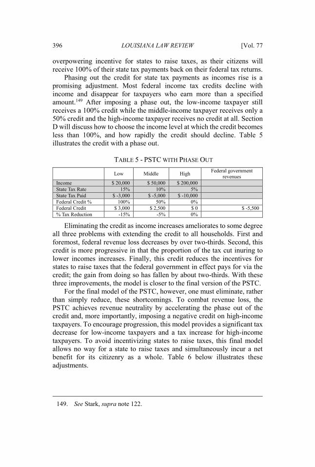
396 LOUISIANA LAW REVIEW [Vol. 77
overpowering incentive for states to raise taxes, as their citizens will receive 100% of their state tax payments back on their federal tax returns.
Phasing out the credit for state tax payments as incomes rise is a promising adjustment. Most federal income tax credits decline with income and disappear for taxpayers who earn more than a specified amount.149 After imposing a phase out, the low-income taxpayer still receives a 100% credit while the middle-income taxpayer receives only a 50% credit and the high-income taxpayer receives no credit at all. Section D will discuss how to choose the income level at which the credit becomes less than 100%, and how rapidly the credit should decline. Table 5 illustrates the credit with a phase out.
TABLE 5 - PSTC WITH PHASE OUT
Low Middle High Federal government revenues
Income $ 20,000 $ 50,000 $ 200,000 State Tax Rate 15% 10% 5% State Tax Paid $ -3,000 $ -5,000 $ -10,000 Federal Credit % 100% 50% 0% Federal Credit $ 3,000 $ 2,500 $ 0 $ -5,500 % Tax Reduction -15% -5% 0%
Eliminating the credit as income increases ameliorates to some degree all three problems with extending the credit to all households. First and foremost, federal revenue loss decreases by over two-thirds. Second, this credit is more progressive in that the proportion of the tax cut inuring to lower incomes increases. Finally, this credit reduces the incentives for states to raise taxes that the federal government in effect pays for via the credit; the gain from doing so has fallen by about two-thirds. With these three improvements, the model is closer to the final version of the PSTC.
For the final model of the PSTC, however, one must eliminate, rather than simply reduce, these shortcomings. To combat revenue loss, the PSTC achieves revenue neutrality by accelerating the phase out of the credit and, more importantly, imposing a negative credit on high-income taxpayers. To encourage progression, this model provides a significant tax decrease for low-income taxpayers and a tax increase for high-income taxpayers. To avoid incentivizing states to raise taxes, this final model allows no way for a state to raise taxes and simultaneously incur a net benefit for its citizenry as a whole. Table 6 below illustrates these adjustments.
149. See Stark, supra note 122.

2016] GIVING CREDIT WHERE CREDIT IS DUE 397
TABLE 6 - PSTC WITH PHASE OUT AND SURCHARGES
Low Middle High Federal government revenues
Income $ 20,000 $ 50,000 $200,000 State Tax Rate 15% 10% 5% State Tax Paid $ -3,000 $ -5,000 $-10,000 Federal Credit % 100% 20% -40% Federal Credit $ 3,000 $ 1,000 $-4,000 $ 0 % Tax Reduction -15% -2% +2%
In this final model, middle-income taxpayers receive a federal income credit for only 20% percent of their state tax payment, as opposed to 50% in the previous iteration. For high-income taxpayers, the “credit” switches from positive to negative. Therefore, instead of receiving a credit on their federal tax returns, these taxpayers will pay an extra tax as part of their federal tax bill. The surcharge will be higher in states that tax the wealthy at relatively low rates.150
As indicated in the last column of Table 6, this version of the PSTC is revenue neutral. Additionally, this final version is also meaningfully progressive. It provides a serious tax cut for low-income taxpayers, a modest one for middle-income payers, and a tax hike for high-income payers. In effect, the PSTC funds a tax cut for low-income households to counteract regressive state taxation and funds this tax cut by raising taxes on high-income households benefiting inequitably from regressive state taxation.
Some might argue that the PSTC goes too far in offsetting regressive state taxation, pointing to the 40% federal tax surcharge imposed on high-income households. This percentage, however, does not apply to total income. Rather, it applies only to state tax payments. The $4,000 tax surcharge imposed on high-income taxpayers amounts to only 2% of their income.
Finally, the final PSTC removes all incentives for states to raise taxes under the belief that the federal tax credit will fully reimburse their citizens. Unlike the 100% PSTC or the phased-out PSTC, the final version offers states no such incentives. Precisely because it is revenue neutral, raising state taxes cannot yield one cent in net benefit to a state’s citizenry as a whole. If a state raises taxes on low-income residents, the PSTC will give those citizens a larger credit but will impose an offsetting tax increase on high-income taxpayers. If a state raises taxes on wealthy residents, the PSTC will remain the same for low- and middle-income households while higher income households will pay the same surcharge in dollar terms, though it will be a lower percent of their state taxes. Even with other, more
150. See discussion infra Part III.D.

398 LOUISIANA LAW REVIEW [Vol. 77
complicated tax increases, the results under the PSTC will always be the same. By design, the final model of the PSTC leans in the direction of progressivity while ensuring that the total tax bills of all state citizens remain unchanged.
D. Explaining Key Choices Made in Constructing the PSTC
To further understand the final PSTC, there are three important factors that require explanation: first, choosing the highest income level to which the PSTC gives a 100% credit; second, calculating the rate at which the credit decreases from 100% to 0% and thereafter into a surcharge; and third, making a final adjustment to achieve a revenue-neutral result. There are multiple ways to determine these factors. Competing demands of efficiency, equity, and ease of administration, among others, make most decisions, such as these, in tax policy contestable. Nevertheless, there are normative justifications for the three choices made regarding the PSTC.
1. Choosing the Income Level at Which the 100% Credit Begins to Phase Out
The PSTC ends the 100% federal income tax credit for state taxes at the income level below which, on average, taxpayers have no net federal tax liability. Because of the federal tax code’s progressive rates along with features like the Earned Income Tax Credit,151 the income at which taxpayers begin paying federal taxes is surprisingly high—approximately at $31,500.152 The idea behind granting a 100% credit up to this income level is that citizens adjudged by Congress too poor to pay even a cent in federal taxes should not pay any state taxes either. One fairly strong, yet valid, assumption behind this choice is that the federal government pays no attention to taxpayers’ state tax payments in setting federal tax rates. The evidence for this assumption is that federal tax law in substance makes no real effort to adjust federal taxes based on taxpayers’ state tax obligations.153 As discussed in Part I, the current deduction for state tax payments, far from aligning federal tax bills with ability to pay, primarily inures to the benefit of wealthier households. Under regressive state tax systems, wealthy households pay less than their fair share of state taxes
151. 26 U.S.C. § 32 (2012). 152. Author’s calculations based on Current Population Survey data. CURRENT POPULATION SURVEY, supra note 30. 153. See discussion supra Part I (arguing that the existing deduction for state taxes on federal tax returns is not at all tied to income or ability to pay).
2016] GIVING CREDIT WHERE CREDIT IS DUE 399
and so have greater ability to pay higher federal taxes; yet, the current federal deduction for state taxes reduces their federal tax liability.
2. Choosing the Rate of the Phase Out
Having determined where the PSTC begins phasing out, the next step is to figure how rapidly the credit percentage should decrease as income increases. In making this determination, the final PSTC model gives ability to pay center stage. The basic idea starts with the observation that the more regressive a state’s tax system, the lower the state tax bill of middle-income and wealthier taxpayers. Lower state tax bills give these subpopulations more financial capacity to receive a lower credit or, for higher incomes, to pay a surcharge on their federal tax return.
This streamlined description conceals a nontrivial issue—that is, measuring the degree of regressivity of a state’s tax regime. One natural way to gauge the regressivity of a tax system is to specify an ideal progressive schedule of rates across income levels and then see how far actual tax rates deviate from this ideal. This method is used in developing the PSTC.
The PSTC phases out the state tax credit in each state based on the difference between the actual and the ideal state tax rates. Starting at the relatively low income where the 100% credit ends, actual rates in every state will exceed the ideal rate because of state tax regressivity. The percent credit for state tax payments declines with rising income based on the convergence of actual and ideal tax rates; the credit reaches zero at the point where the actual rate equals the ideal rate. Those with higher incomes, for which actual state tax rates are less than the ideal rates, pay a surcharge that increases in proportion to the gap between the ideal tax rate the taxpayer should be paying and the lower actual rate the payer pays as a result of regressive state taxation.
This scheme depends on specification of the ideal state tax rate schedule. Again, there are multiple ways to make this choice. For example, one could start with some axioms about fair distribution and derive an ideal rate deductively. In contrast, one could estimate empirically the marginal value of one dollar across incomes and set the ideal rate to maximize the total value of national income.154
154. This does sound fairly close to performing interpersonal utility comparisons, a taboo for many efficiency-fixated economists. Many other economists, however, and perhaps most laymen lose little sleep claiming that an additional dollar for a starving child has greater individual, and of course greater social, utility than an additional dollar for a billionaire’s bequest to her children. See generally John C.
400 LOUISIANA LAW REVIEW [Vol. 77
The PSTC takes a different, political economy tack to selecting an ideal state tax schedule. As discussed in Part I, the mobility of citizens and their income imposes at least some constraints on states’ abilities to impose progressive taxes. Changing national citizenship is much more expensive, however, and so the federal government faces a much weaker mobility constraint on its ability to tax progressively. If one has even a moderate belief in the ability of elected governments to reflect the electorate’s preferences, the current and fairly progressive federal income tax schedule possesses an imprimatur of democratic legitimacy. On this basis, the PSTC uses a modified version of the current federal income tax schedule as the ideal state tax schedule.
Modification is necessary due to the difference in the revenue raised from each state by the federal government and by the state itself. If a state raised exactly as much revenue from its citizens as the federal government raised, then the ideal state tax schedule would be exactly the same as the federal tax rate schedule. If, however, a state raises less tax revenue than its citizens pay in federal income taxes, the ideal tax rates for the state must be scaled down in order to match its lower revenue needs. Conversely, if a state raises more revenue from its citizens than the national government raises, the state’s ideal rates must be a scaled-up version of federal rates.
One solution takes care of both problems. To determine a state’s ideal rate structure, one can multiply federal rates by the ratio of state tax revenues to federal income tax revenues from a state’s citizens. For example, if a state’s total tax revenue was $3 billion and the federal government raised $4 billion in income taxes from the state’s citizens, then the ideal state tax rate at a given income level would equal 75% of the federal income tax rate. Furthermore, this would mean that if the effective federal income tax rate for those with incomes of $100,000 was 40%, the ideal state tax rate for purposes of computing the PSTC would be three-fourths of 40%, or 30%. This methodology yields lower ideal rate schedules in states with lower overall tax revenues, and higher ideal rate schedules in states with higher overall taxes. Thus in effect, if not in form, tax rates will vary from state to state. Questions concerning the constitutionality of such a tax system are addressed in Part V.
Before the final step, it is helpful to summarize the steps described so far to delineate the PSTC. First, a state’s taxpayers who are at or below the income level at which a household pays no federal income taxes receive a 100% credit for state taxes paid. Second, between this relatively low income level and the much higher income level at which declining actual
Harsanyi, Interpersonal Utility Comparisons, in 4 THE NEW PALGRAVE DICTIONARY OF ECONOMICS 529 (Steven N. Durlauf & Lawrence E. Blume eds., 2d ed. 2008).

2016] GIVING CREDIT WHERE CREDIT IS DUE 401
state tax rates fall to the level of ideal state rates, the PSTC phases out from 100% to 0%. Finally, at higher incomes, for which actual state tax rates are below ideal rates, households pay a surcharge, calculated as a percent of their state tax payments, based on the positive gap between their ideal and their actual tax rates.
3. Ensuring Revenue Neutrality
The PSTC as constructed does an excellent job of eliminating most of states’ incentives to increase their taxes and have the federal government pay some portion of these taxes indirectly via the credit. It is also significantly more progressive than either the current deduction or a simple 100% credit for all taxpayers. There is, however, no guarantee that the PSTC, crafted up to this point, is revenue neutral. Indeed, calculations behind the empirical estimates of the PSTC’s impact across states and income levels presented in Part IV and the Appendices show that there would be a revenue shortfall in every state.155
Raising revenue requires some combination of decreasing the credit for lower income earners and increasing the surcharge for higher income earners. The now decades-long rise in inequality weighs heavily in favor of higher surcharges at the top of the income distribution. As documented in Figure 1 and Figure 2, real incomes for the lower and middle classes have remained essentially flat for decades. In contrast, incomes in the top 10% and the top 1% have grown spectacularly. To paraphrase bank robber Willie Sutton, we should impose higher surcharges on the wealthy because that is where most income is going.156
To achieve revenue neutrality, then, the PSTC increases the surcharge rate on higher incomes in each state proportionally so that the proposal is revenue neutral. This extra dose of taxation at the top of the income distribution is justified based on the sharp increase in those incomes over the last few decades. Note that the PSTC has a symmetric, converse bend at the bottom of the income distribution. Progressivity suggests that a household with $5,000 needs more tax relief than one with $10,000, but the PSTC gives them the same percent benefit as percent of state taxes
155. Intermediate results obtained in calculating the data appear in Appendices A & B. 156. Sutton supposedly replied, when asked why he robbed banks, “Because that is where the money is.” Willie Sutton, WIKIPEDIA, https://en.wikipedia.org /wiki/Willie_Sutton [https://perma.cc/EM67-ML97] (last visited Nov. 18, 2016). Sutton, however, denies having ever made this statement. See generally WILLIE SUTTON & EDWARD LINN, WHERE THE MONEY WAS: THE MEMOIRS OF A BANK ROBBER 160 (1976).
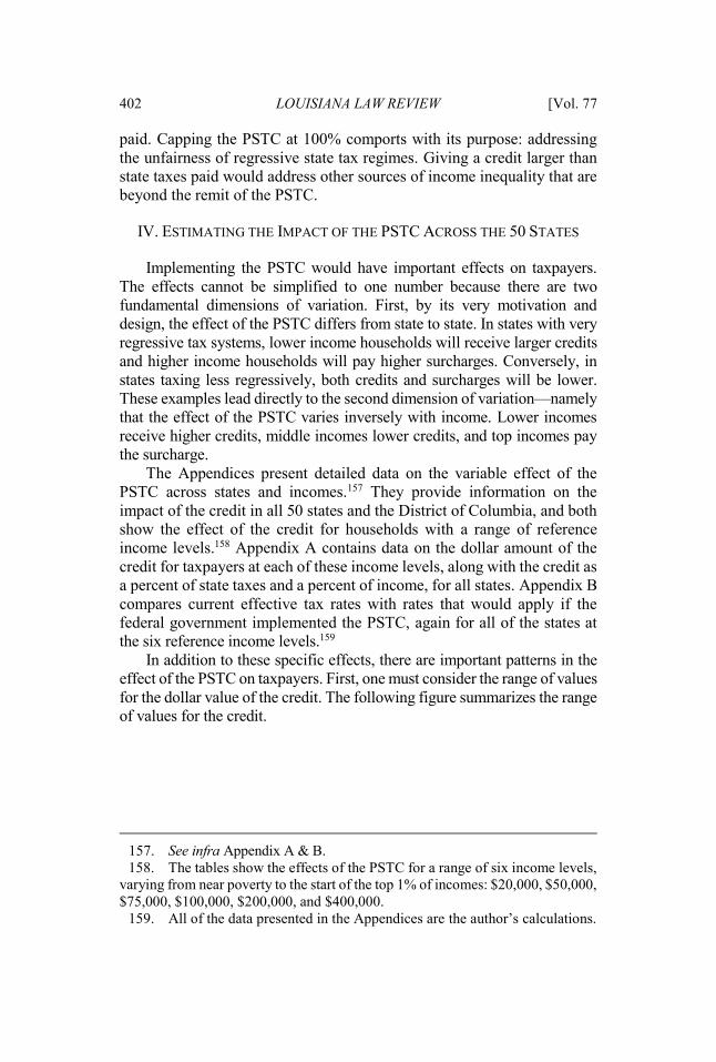
402 LOUISIANA LAW REVIEW [Vol. 77
paid. Capping the PSTC at 100% comports with its purpose: addressing the unfairness of regressive state tax regimes. Giving a credit larger than state taxes paid would address other sources of income inequality that are beyond the remit of the PSTC.
IV. ESTIMATING THE IMPACT OF THE PSTC ACROSS THE 50 STATES
Implementing the PSTC would have important effects on taxpayers. The effects cannot be simplified to one number because there are two fundamental dimensions of variation. First, by its very motivation and design, the effect of the PSTC differs from state to state. In states with very regressive tax systems, lower income households will receive larger credits and higher income households will pay higher surcharges. Conversely, in states taxing less regressively, both credits and surcharges will be lower. These examples lead directly to the second dimension of variation—namely that the effect of the PSTC varies inversely with income. Lower incomes receive higher credits, middle incomes lower credits, and top incomes pay the surcharge.
The Appendices present detailed data on the variable effect of the PSTC across states and incomes.157 They provide information on the impact of the credit in all 50 states and the District of Columbia, and both show the effect of the credit for households with a range of reference income levels.158 Appendix A contains data on the dollar amount of the credit for taxpayers at each of these income levels, along with the credit as a percent of state taxes and a percent of income, for all states. Appendix B compares current effective tax rates with rates that would apply if the federal government implemented the PSTC, again for all of the states at the six reference income levels.159
In addition to these specific effects, there are important patterns in the effect of the PSTC on taxpayers. First, one must consider the range of values for the dollar value of the credit. The following figure summarizes the range of values for the credit.
157. See infra Appendix A & B. 158. The tables show the effects of the PSTC for a range of six income levels, varying from near poverty to the start of the top 1% of incomes: $20,000, $50,000, $75,000, $100,000, $200,000, and $400,000. 159. All of the data presented in the Appendices are the author’s calculations.
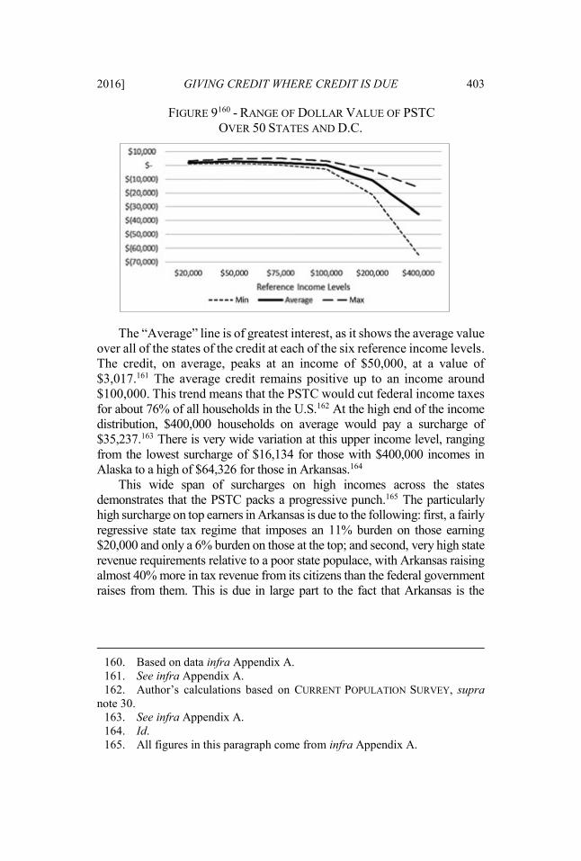
2016] GIVING CREDIT WHERE CREDIT IS DUE 403
FIGURE 9160 - RANGE OF DOLLAR VALUE OF PSTC OVER 50 STATES AND D.C.
The “Average” line is of greatest interest, as it shows the average value over all of the states of the credit at each of the six reference income levels. The credit, on average, peaks at an income of $50,000, at a value of $3,017.161 The average credit remains positive up to an income around $100,000. This trend means that the PSTC would cut federal income taxes for about 76% of all households in the U.S.162 At the high end of the income distribution, $400,000 households on average would pay a surcharge of $35,237.163 There is very wide variation at this upper income level, ranging from the lowest surcharge of $16,134 for those with $400,000 incomes in Alaska to a high of $64,326 for those in Arkansas.164
This wide span of surcharges on high incomes across the states demonstrates that the PSTC packs a progressive punch.165 The particularly high surcharge on top earners in Arkansas is due to the following: first, a fairly regressive state tax regime that imposes an 11% burden on those earning $20,000 and only a 6% burden on those at the top; and second, very high state revenue requirements relative to a poor state populace, with Arkansas raising almost 40% more in tax revenue from its citizens than the federal government raises from them. This is due in large part to the fact that Arkansas is the
160. Based on data infra Appendix A. 161. See infra Appendix A. 162. Author’s calculations based on CURRENT POPULATION SURVEY, supra note 30. 163. See infra Appendix A. 164. Id. 165. All figures in this paragraph come from infra Appendix A.

404 LOUISIANA LAW REVIEW [Vol. 77
poorest state in the U.S., based on either average or median income.166 Under the PSTC, surcharges on a relatively small pool of wealthy Arkansans must match the subsidy due to a very large group of lower income households. At the other extreme, the low surcharge on high-income Alaskans is due largely to the fact that over 91% of the state’s revenue comes not from taxes on citizens, but rather from taxes on the extraction of gas, oil, and minerals and taxes on the corporations that engage in extraction.167 Thus, light state revenue needs mean that Alaskans pay very little in state taxes, and thus the PSTC provides small credits for low-income households and imposes correspondingly low surcharges on high-income households.
Figure 9 seems to suggest that the PSTC has very small effects on the vast majority of American households with incomes below $100,000. That data, however, is in raw dollars. The burdens of taxes usually are measured in percent terms. This gives a more accurate gauge of a tax’s real impact, as using percentages adjusts for income differences. A $1,000 tax on someone with an income of $20,000 has a much different effect than the same $1,000 tax on someone with a $200,000 income. A 5% tax on both seems a better, if still imperfect, way to produce nearly equivalent burdens. On this percent of income basis, the benefits of the PSTC at the low and high ends of the income distribution, on average, are mirror images of one another. For example, those making $20,000 enjoy a tax benefit of about 10%, while those making $400,000 suffer about a 9% tax increase.
166. Arkansas has an average income of about $61,300 and a median income of $44,300. The national averages are $78,255 and $57,040. Author’s calculations based on the CURRENT POPULATION SURVEY, supra note 30. 167. TAX DIV., ALASKA DEP’T OF REVENUE, ANNUAL REPORT 9 (2014), http: //www.tax.alaska.gov/programs/documentviewer/viewer.aspx?1139r [https://perma .cc/HK2S-AHMX].

2016] GIVING CREDIT WHERE CREDIT IS DUE 405
FIGURE 10168 - RANGE OF PSTC AS PERCENT OF INCOME OVER 50 STATES AND D.C.
This figure shows that in percentage terms, the burden imposed by the PSTC on wealthy taxpayers is roughly equal to the benefit conferred on poorer taxpayers. Moreover, the variation in these benefits and burdens across states is fairly consistent at all reference income levels, as indicated by the “Min” and “Max” lines closely sandwiching the “Average” line in Figure 10.
For households earning $20,000, the PSTC ranges only from 5.7% in Delaware to a maximum of 16.6% in Washington.169 The appearance of these two states at the extremes should come as no surprise. Delaware has one of the least regressive state tax regimes in the nation, and hence there is relatively little work for the PSTC to do.170 Recall that Washington, on the other hand, has by some measures the most regressive state tax system, and so the PSTC provides a large benefit to low-income taxpayers in the state.171
At the other extreme, the surcharge on $400,000 incomes ranges from 4% in Alaska to 16% in Arkansas.172 This range is almost precisely equal to the range of effects at $20,000, again suggesting that the PSTC has nearly equal impacts on high and low incomes. Inspecting Figure 10 at intermediate incomes shows much the same phenomenon, and the figures
168. Based on data infra Appendix A. 169. See infra Appendix A. 170. See supra Figure 8. 171. See supra Figure 6 & Figure 8. 172. See infra Appendix A.
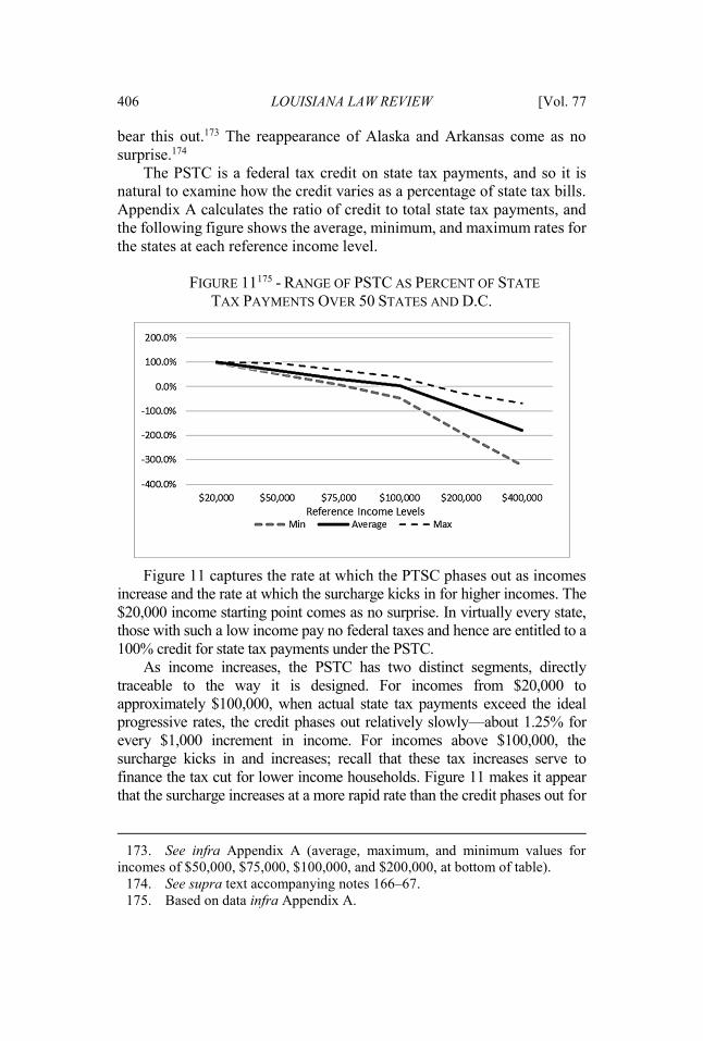
406 LOUISIANA LAW REVIEW [Vol. 77
bear this out.173 The reappearance of Alaska and Arkansas come as no surprise.174
The PSTC is a federal tax credit on state tax payments, and so it is natural to examine how the credit varies as a percentage of state tax bills. Appendix A calculates the ratio of credit to total state tax payments, and the following figure shows the average, minimum, and maximum rates for the states at each reference income level.
FIGURE 11175 - RANGE OF PSTC AS PERCENT OF STATE
TAX PAYMENTS OVER 50 STATES AND D.C.
Figure 11 captures the rate at which the PTSC phases out as incomes increase and the rate at which the surcharge kicks in for higher incomes. The $20,000 income starting point comes as no surprise. In virtually every state, those with such a low income pay no federal taxes and hence are entitled to a 100% credit for state tax payments under the PSTC.
As income increases, the PSTC has two distinct segments, directly traceable to the way it is designed. For incomes from $20,000 to approximately $100,000, when actual state tax payments exceed the ideal progressive rates, the credit phases out relatively slowly—about 1.25% for every $1,000 increment in income. For incomes above $100,000, the surcharge kicks in and increases; recall that these tax increases serve to finance the tax cut for lower income households. Figure 11 makes it appear that the surcharge increases at a more rapid rate than the credit phases out for
173. See infra Appendix A (average, maximum, and minimum values for incomes of $50,000, $75,000, $100,000, and $200,000, at bottom of table). 174. See supra text accompanying notes 166–67. 175. Based on data infra Appendix A.

2016] GIVING CREDIT WHERE CREDIT IS DUE 407
lower incomes. This appearance, however, is misleading. The reference income values on the horizontal axis are not spaced proportionally. There is, for example, as much space between $20,000 and $50,000 as there is between $200,000 and $400,000. In fact, the surcharge on higher incomes rises by only about 0.6% on average over all states.
The data presented in Appendix B gives a broader, more “bottom line” summary of the effect of the PSTC. It compares effective tax rates under the credit to current prevailing rates, providing the best summary measure of the differential benefits bestowed by and burdens imposed by the PSTC.
FIGURE 12176 - AVERAGE FEDERAL INCOME TAX RATES
OVER ALL STATES, CURRENT V. PSTC
In Figure 12, first note that the average tax rate curve for the PSTC
has a steeper slope than its counterpart under the current tax code. This means that it has lower rates at low incomes and higher rates at high incomes. In a word, the PSTC is more progressive. This progressivity, of course, is by design, but it is worth studying in a bit more detail. Averaging across all jurisdictions, the PSTC reduces the tax bill of those earning $20,000 by slightly more than 10%. At the other extreme, it increases the tax bill of those earning $400,000 by about 6.3% averaged across the states. Finally, note again that the “crossover” income level is $100,000, and those making less enjoy a tax cut under the PSTC, while those making more pay more in federal income taxes. As the four preceding figures show, 76% of American households earning less than $100,000 would get some relief from regressive state taxation under the PSTC.177
176. Based on data infra Appendix B. 177. See supra text accompanying note 162.

408 LOUISIANA LAW REVIEW [Vol. 77
V. THE PSTC AND THE CONSTITUTION’S UNIFORMITY CLAUSE
The calculations and illustrations discussed above highlight the fact that under the PSTC, effective tax rates will differ from state to state. The fact that the federal income tax surcharge for state income tax payments will vary from state to state, in proportion to the regressivity of the state’s tax code, means that otherwise similarly situated individuals who live in states with different tax rates will not face equal federal tax liability. The goal of the PSTC is progressivity, and so higher income taxpayers from those states that tax most regressively will face higher tax bills—in effect higher tax rates, in both marginal and average terms. Such taxpayers might think of challenging the PSTC under the Uniformity Clause of the Constitution, which provides that “Congress shall have Power To lay and collect Taxes, Duties, Imposts and Excises . . . but all Duties, Imposts and Excises shall be uniform throughout the United States.”178
Perhaps the easiest defense of the PSTC would be its formal similarity to the current deduction for state tax payments. Although the deduction is regressive, it in effect makes federal tax liability and tax rates a function of state taxes. The deduction has existed since the beginning of the modern federal income tax,179 and one cannot find even a single argument that it violates the Uniformity Clause. Credits do not seem to differ from deductions in constitutional dimensions, and so the long acceptance of the state tax deduction provides a safe harbor for the PSTC from a Uniformity Clause challenge.
In substance, however, the PSTC is quite different from the deduction. In particular, the surcharge on higher incomes has no analog in the current deduction. Although packaged within the structure of what is labeled a “credit,” a court applying substance over form might well label it a tax. As such, it would be a tax that varied from state to state, arguably a violation of the Uniformity Clause.
This Part ultimately concludes that as a matter of constitutional doctrine, there is no problem with the PSTC. The argument proceeds in a somewhat unorthodox fashion. Instead of demonstrating the constitutionality of the PSTC itself, this Part shows that a federal income tax with rates that vary from state to state in service of progressivity does not generally violate the
178. U.S. CONST. art. I, § 8, cl. 1. 179. See TAX POL’Y CTR., THE TAX POLICY BRIEFING BOOK: A CITIZENS’ GUIDE FOR THE 2012 ELECTION AND BEYOND IV, at 1–18 (“State and local taxes have been deductible since the inception of the federal income tax in 1913 . . . .”).

2016] GIVING CREDIT WHERE CREDIT IS DUE 409
Uniformity Clause.180 The constitutionality of the PSTC then follows as a special case of this general result.
Uniformity Clause precedents are few. In the first substantive discussion of the Uniformity Clause, The Head Money Cases,181 shipping lines transporting immigrants from Europe to the U.S. objected to paying “head” tax on each immigrant whom they brought into the U.S.182 They argued that because the tax fell disproportionately on a few states with busy ports, and because it did not apply to inland immigrants, it violated the Uniformity Clause.183 The Court dismissed the challenge in rather curt fashion, noting that “[p]erfect uniformity and perfect equality of taxation, in all the aspects in which the human mind can view it, is a baseless dream.”184 As brief and cryptic as it is, the Court’s standard for applying the Uniformity Clause has survived: “[A] tax is uniform when it operates with the same force and effect in every place where the subject of it is found.”185 To oversimplify, this geographic rule seems to say federal taxes comply with the Uniformity Clause even if the base of the tax is not distributed uniformly across the nation, as long as the rate charged to taxpayers does not depend on their state of residence.
Taken at face value, The Head Money Cases do seem in tension with state-varying tax rates. Imagine Taxpayer A from Alabama and Taxpayer W from Wyoming have the same income in each category, number of dependents, size of deductions, and credits. Any regime that imposed different taxes on these two individuals does not seem “uniform.”
The legal standard articulated in Knowlton v. Moore,186 the next and still-leading Uniformity Clause case, seems only to reinforce the geography rule of The Head Money Cases. Knowlton involved a Uniformity Clause challenge to a federal estate tax under which variations in state law would lead to differential tax liability for similarly situated individuals in different states.187 The Court declared that during the Founding Era, the phrase “uniform throughout the United States” was used “always with reference purely to a geographical uniformity and as
180. This argument is developed in another more technical paper, which proposes varying federal income tax rates from state to state to undo the regressivity of state taxation. Eric Kades, Corrective Progressivity (forthcoming 2016), https://papers .ssrn.com/sol3/papers.cfm?abstract_id=2621356 [https://perma.cc/92C8-S58C]. 181. Edye v. Robertson, 112 U.S. 580 (1884). 182. Id. at 588. 183. Id. at 594–95. 184. Id. at 595. 185. Id. at 594. 186. 178 U.S. 41 (1900). 187. Id. at 43.

410 LOUISIANA LAW REVIEW [Vol. 77
synonymous with the expression ‘to operate generally throughout the United States.’”188 The Court reiterated that this geographic uniformity does not require taxing only those sources that were spread evenly across the states; “what the Constitution commands is the imposition of a tax by the rule of geographical uniformity, not that in order to levy such a tax objects must be selected which exist uniformly in the several states.”189
Although this standard sounds antithetical to state-varying tax rates, the facts and the outcome of Knowlton suggest less of a dissonance. The opinion offers precious few hints about the exact nature of state laws that would have caused tax consequences to differ by state; however, those details do not seem important. Regardless, the parallel between the federal estate tax at issue in Knowlton and state-varying federal income tax rates is striking: varying state laws drive varying federal tax consequences. Knowlton held that such state-law-driven variation in federal tax liability does not violate the Uniformity Clause.190 The Court did not see fit to focus on this facet of the case, but the holding nonetheless suggests that a federal tax can impose differential tax consequences based on state law.
Perhaps of even greater import, Knowlton explained the policy reason for the uniformity requirement—and the PSTC is entirely consistent with the purpose of the clause. The Court said the geographic test from The Head Money Cases “look[s] to the forbidding of discrimination as between the states, by the levying of duties, imposts, or excises upon a particular subject in one state and a different duty, impost, or excise on the same subject in another.”191 In summarizing debates over the Uniformity Clause and related provisions of the draft Constitution, the Court asserted that the “sole and the only question” was “discrimination as regards states which might arise from a greater or lesser proportion of any tax being paid within the geographical limits of a particular state.”192 In a manner of speaking, the Knowlton Court describes the Uniformity Clause as a sort of taxation equal protection clause for states, a provision to prevent a majority block of states from imposing a disproportionate share of federal revenue needs on an outvoted minority.
The Supreme Court’s most recent Uniformity Clause decision, U.S. v. Ptasynski,193 reaffirms this theme and simultaneously grants Congress wide discretion to enact tax laws. Ptasynski upheld provisions of the Windfall Profits Tax on Oil that exempted Alaskan oil extracted from 188. Id. at 96. 189. Id. at 108. 190. Id. at 106–09. 191. Id. at 89. 192. Id. at 96. 193. 462 U.S. 74 (1983).

2016] GIVING CREDIT WHERE CREDIT IS DUE 411
within the Arctic Circle.194 The Court cited Justice Story at length on the anti-discriminatory purpose of the Uniformity Clause:
[The purpose of the Clause] was to cut off all undue preferences of one State over another in the regulation of subjects affecting their common interests. Unless duties, imposts, and excises were uniform, the grossest and most oppressive inequalities, vitally affecting the pursuits and employments of the people of different States, might exist. The agriculture, commerce, or manufactures of one State might be built up on the ruins of those of another; and a combination of a few States in Congress might secure a monopoly of certain branches of trade and business to themselves, to the injury, if not to the destruction, of their less favored neighbors.195
When deciding if a federal tax helps one group of states at the expense of another, Congress can entirely avoid the application of the Uniformity Clause simply by not defining the subject of the tax in geographic terms.196 Moreover, even if Congress chooses to define a tax geographically, the levy will run afoul of the Uniformity Clause only if a court finds “actual geographic discrimination.”197 On the facts of the case, the Court found that the exemption granted for oil pumped from the most northern wells of Alaska was justified based on “the disproportionate costs and difficulties” incurred in harvesting oil in such a cold and remote region.198 It emphasized that Congress created geographically driven differential tax treatment based on “neutral factors” and also evidenced no intent to “offend the purpose of the [Uniformity] Clause.”199
Both of these rationales provide strong reasons to find that a federal income tax with rates that vary from state to state based on “neutral factors” does not violate the Uniformity Clause. Starting with the purpose of the Clause, federal tax provisions in the service of progressivity are not inconsistent or even in tension with the “tax equal protection” rationale for including the Clause in the Constitution. To use the PSTC as an example, it in no way discriminates against any particular state. It is revenue neutral, so it does not impose an additional tax burden on any state. Moreover, it
194. Id. at 86. 195. Id. at 81 (quoting 1 JOSEPH STORY, COMMENTARIES ON THE CONSTITUTION OF THE UNITED STATES § 957 (T. Cooley ed. 1873)). 196. Id. at 84. 197. Id. at 85. 198. Id. 199. Id.
412 LOUISIANA LAW REVIEW [Vol. 77
does not single any state out for differential treatment. States that do not like the effect of the PSTC on their citizen’s federal tax bills are entirely free to abandon their tax regime and adopt that of another state that they think is treated more favorably under the PSTC, or to adopt an entirely novel state tax system—perhaps one that is actually progressive.
Second, the motivation for enacting progressive federal tax provisions is simply fairness in taxation. “Ability to pay” is a common element of general tax fairness norms, and the Supreme Court has said that it is a legitimate reason for disparate treatment of taxpayers. In Knowlton, the Court cited English precedents dating back to 1643 that justified taxes on a wide variety of items and asserted that in the early Republic “taxes were frequently laid from a consideration of the presumed ability of the owner to pay the tax.”200 Thus one of the core motives for progressive taxation is older than the nation itself, providing a “neutral” foundation that should immunize such levies from a Uniformity Clause challenge. The Supreme Court has repeatedly stated that ability to pay is a legitimate ground for imposing disparate tax burdens.201
Both legislation202 and case law offer precedents for measures that make federal tax liability depend on state law. Three examples provide illustrations. First, in Florida v. Mellon,203 the Court upheld a federal income tax that granted a deduction of up to 80% for any state inheritance tax paid on a legacy. Florida’s constitution contained a clause barring the state legislature from adopting an inheritance tax,204 but this made no difference to the Supreme Court. The Court rejected the contention that Congress was coercing states into enacting their own inheritance tax205 and without reservation accepted the notion that differing state laws could cause differing federal tax liability without running afoul of the
200. Id. at 89–91. 201. See, e.g., Greenough v. City of Newport, 331 U.S. 486 (1947) (upholding tax on out-of-state intangible assets in part based on ability to pay); New York ex rel. Cohn v. Graves, 300 U.S. 308, 313 (1937) (upholding tax on rents earned out of state, in part on grounds that tax was “apportioned to the ability of the taxpayer to pay it”); Fox v. Standard Oil Co., 294 U.S. 87, 101 (1935) (upholding higher tax rate for chains of gasoline retailers based in part on “the capacity to pay”). 202. Other Internal Revenue Code provisions that create tax burdens that vary based on a taxpayer’s state of residence include the deductibility of property taxes, 26 U.S.C. § 164(a)(1) (2012), and the deductibility of interest on state and local bonds given that interest rates vary across the states. Id. § 103. 203. 273 U.S. 12 (1927). 204. Id. at 15. 205. Id. at 16.

2016] GIVING CREDIT WHERE CREDIT IS DUE 413
Uniformity Clause.206 The Court voiced a wide tolerance for disparate impact of federal tax provisions across the several states:
The contention that the federal tax is not uniform, because other states impose inheritance taxes while Florida does not, is without merit. Congress cannot accommodate its legislation to the conflicting or dissimilar laws of the several states, nor control the diverse conditions to be found in the various states, which necessarily work unlike results from the enforcement of the same tax.207
The tax at issue in Mellon is not exactly analogous to issues surrounding the PSTC, but it shares the core similarity of reducing a federal tax liability based on a state tax liability. The opinion stands as a strong precedent for the constitutionality of varying effective federal tax rates based on divergent state tax provisions.
The second precedent, Poe v. Seaborn,208 provides additional helpful language. Poe held that federal tax authorities could assert substance over form and impute half of the income from a married couple’s community property to the wife even though formally the husband held title to the assets.209 In upholding the federal government’s approach against a Uniformity Clause challenge, the Court said that “differences of state law, which may bring a person within or without the category designated by Congress as taxable, may not be read into the Revenue Act to spell out a lack of uniformity.”210 The Court cited Florida v. Mellon on this point, buttressing the argument that federal tax liability may vary with state law.211
Next, there is the aforementioned longstanding practice212 of making state tax payments deductible on federal tax returns. The usual rationale for permitting taxpayers to deduct state and local tax payments from their federal taxable income is ability to pay—a taxpayer cannot use the same dollars to pay both federal and state taxes. As misguided as this perspective might be, it nonetheless has stood the test of time and has never been subject to constitutional challenge.
206. Id. at 17. 207. Id. 208. 282 U.S. 101 (1930). 209. Id. at 118. 210. Id. at 117–18. 211. Id. 212. Deductibility of state and local taxes from federal income taxation dates back to the Civil War era. William Turner, Evaluating Personal Deductions in an Income Tax—The Ideal, 66 CORNELL L. REV. 262, 264–65 (1981).

414 LOUISIANA LAW REVIEW [Vol. 77
More generally, the effects of other federal legal regimes vary based on state law. Perhaps most prominent is bankruptcy law, in which a foundational principle is that federal bankruptcy law looks to state law to define property rights—and these property rights vary from state to state.213 To give a more specific example, the Bankruptcy Code gives debtors the choice to protect “exempt” property from creditors based on either a federal definition of exemptions or their state’s definition.214 The Supreme Court upheld this regime to a challenge under the Bankruptcy Code’s Uniformity Clause.215
Indeed, a moment’s reflection makes clear that state and local law have myriad differential effects on federal income tax liability. To give but one very widespread example, some local zoning laws contain severe limitations on the development of property.216 These restrictions can have a huge effect on both income and capital gains from the property, yet no one has questioned the constitutionality of zoning ordinances on Uniformity Clause grounds. Though it may not be widely recognized, federal income taxes vary from state to state based on an unexpectedly large array of state laws. Unless courts intend to subject these myriad laws to Uniformity Clause review, the constitutionality of the PSTC is an easy call.
CONCLUSION
Although the PSTC does not pose any serious constitutional questions, it is difficult to deny that it proposes a significant change to the federal income tax code. Major innovations should address major problems. When the total state tax burden on poor households in the states are on average
213. Butner v. U.S., 440 U.S. 48 (1979) (holding that state law, not federal equity rule, determined rights to rents collected between declaration of bankruptcy and foreclosure sale). 214. 11 U.S.C. § 522 (2012). Note all states permit debtors to elect the federal exemptions. 215. Hanover Nat’l Bank v. Moyses, 186 U.S. 181 (1902); see also Stellwagen v. Clum, 245 U.S. 605 (1918). The Bankruptcy Clause gives Congress the power “[t]o establish a uniform Rule of Naturalization, and uniform Laws on the subject of Bankruptcies throughout the United States.” U.S. CONST. art. I, § 8, cl. 4. For a convincing argument that the Framers intended to attach a similar uniformity requirement to Congress’s power under the commerce clause, see Thomas B. Colby, Revitalizing the Forgotten Uniformity Constraint on the Commerce Power, 91 VA. L. REV. 249, 301–24 (2005). 216. See, e.g., Village of Euclid v. Ambler Realty Co., 272 U.S. 365 (upholding local zoning ordinance despite 38% reduction in property’s value).

2016] GIVING CREDIT WHERE CREDIT IS DUE 415
twice as high as on wealthy households and range as high as eight times higher, there is a strong indication of unfairness in state taxation.217
The states are indeed laboratories of democracy,218 but sometimes their experiments fail, and those star-crossed programs can persist for decades and even centuries. Perhaps the most prominent example is the regime of racial segregation imposed by whites throughout the South after the end of the Reconstruction Era in 1876. The “Jim Crow” laws discriminating against African Americans maintained their vitality for almost 100 years, and there were few signs that normal political forces in southern states would solve the problem. It was only with the intervention of the federal government, via a string of path-breaking civil rights statutes,219 that de jure segregation began to disappear.
The civil rights legislation of the 1960s is far from a perfect analogy for the regressive condition of state taxation. In particular, the political failure that produced racial segregation—white majority oppression of the black minority—was transparent; the explanation for widespread regressive state taxation is far from clear. The best study to date found precious little correlation between suspected explanatory variables like a state’s political leanings or a state’s income inequality.220 In at least some states, it appears that nothing more than sticky old court rulings that a state’s constitution bars an income tax explain regressive tax systems.221
It was conceivable, though highly unlikely, that all of the Jim Crow states would have ended de jure segregation via normal political processes. Even if this would have happened eventually, segregation inflicted great injustices across a broad swathe of the population on a daily basis. Here 217. DAVIS ET AL., supra note 7, at 3. The state of Washington has the largest difference between rates paid by the bottom 20% and the top 1%: 16.8% versus 2.4% (16.8/2.4 ≈ 7). Id. at 123. 218. New State Ice Co. v. Liebmann, 285 U.S. 262, 311 (1932) (Brandeis, J., dissenting) (“It is one of the happy incidents of the federal system that a single courageous state may, if its citizens choose, serve as a laboratory; and try novel social and economic experiments without risk to the rest of the country.”). 219. See, e.g., Civil Rights Act of 1964, Pub. L. No. 88-352, 78 Stat. 241 (codified in scattered sections of 42 U.S.C.); Voting Rights Act of 1965, Pub. L. No. 89-110, 79 Stat. 437 (codified at 52 U.S.C. § 10101 et seq.); Civil Rights Act of 1968, Pub. L. No. 90-284, 82 Stat. 73 (codified in scattered sections of 42 U.S.C.). 220. Chernick, supra note 137, at 102. 221. See Culliton v. Chase, 25 P.2d 81 (Wash. 1933) (finding income tax adopted by popular vote violated the Washington State Constitution’s Uniformity Clause); Evans v. McCabe, 52 S.W.2d 159 (Tenn. 1932) (holding income tax violated provision of Tennessee Constitution that expressly permitted a tax on income from stocks and bond, thus impliedly disallowing an income tax on any other type of income).

416 LOUISIANA LAW REVIEW [Vol. 77
there are strong parallels to regressive state taxation. There is little if any evidence that even a single state is focusing on serious reform of its regressive tax system; indeed, the problem is getting worse.222 Moreover, the injustice is flagrant. Families below the poverty line in many states face state tax rates at least twice as high as the state’s wealthiest households. Rates paid by middle-class families are only modestly less extreme. Nobody has proffered a justification for allocating the burden of funding public goods so disproportionately on the poor. This is not surprising, as there is no justification.
It is against this background that the PSTC has elements of civil rights legislation, for the poor and middle classes instead of for oppressed minorities. It offers a federal solution to what appears to be fundamental political failings in state politics. Every state taxes regressively despite the fact that regressive taxation has no friends anywhere on the political spectrum. There is neither rhyme nor reason to the pattern of regressivity in state taxation. State political leanings, inequality in state incomes, history, and all other plausible explanatory variables explain precious little of the variations in state tax policy.
The PSTC is an innovative measure for fixing the regressivity of every state tax system. It uses a well-established federal income tax tool, a tax credit, and deploys the credit in a way consistent with many other existing tax credits—progressively. Perhaps of greatest moment, it simultaneously fixes the broken regressive tax schemes in all 50 states and the District of Columbia. Finally, it is politically feasible. It does not seem a fantasy to imagine a majority of non-wealthy voters embracing a tax measure that benefits the 76% of American households with incomes below $100,000.223
222. See supra Figure 7 (showing on average state taxes became more regressive between 1996 and 2014). 223. See supra text accompanying note 162.

2016] GIVING CREDIT WHERE CREDIT IS DUE 417
APPENDIX A. CREDIT IN DOLLAR AMOUNT AND AS PERCENT OF STATE TAXES AND INCOME, BY STATE
A = Credit/surcharge B = Credit as percent of state taxes C = Credit as percent of income
$ 20,000 $ 50,000 $ 75,000 $ 100,000 $ 200,000 $ 400,000
AL
A $ 2,044 $ 3,136 $ 1,738 $ 54 $ (13,364) $ (37,713) B 100.0% 66.0% 28.0% 0.7% -130.4% -243.2% C 10.2% 6.3% 2.3% 0.1% -6.7% -9.4%
AK
A $ 1,429 $ 1,699 $ 944 $ 35 $ (4,844) $ (16,134) B 100.0% 66.7% 29.8% 1.0% -93.8% -167.7% C 7.1% 3.4% 1.3% 0.0% -2.4% -4.0%
AZ
A $ 2,534 $ 3,495 $ 2,279 $ 606 $ (11,066) $ (37,203) B 100.0% 73.9% 35.9% 7.9% -89.2% -187.7% C 12.7% 7.0% 3.0% 0.6% -5.5% -9.3%
AR
A $ 2,391 $ 3,736 $ 997 $ (2,765) $ (21,013) $ (64,926) B 100.0% 67.5% 13.6% -30.1% -162.7% -268.0% C 12.0% 7.5% 1.3% -2.8% -10.5% -16.2%
CA
A $ 2,105 $ 2,764 $ 1,792 $ 603 $ (4,883) $ (24,011) B 100.0% 64.8% 30.4% 8.0% -29.6% -68.4% C 10.5% 5.5% 2.4% 0.6% -2.4% -6.0%
CO
A $ 1,779 $ 2,813 $ 2,160 $ 1,190 $ (6,984) $ (26,166) B 100.0% 65.0% 36.1% 15.8% -56.9% -138.4% C 8.9% 5.6% 2.9% 1.2% -3.5% -6.5%
CT
A $ 2,230 $ 2,603 $ 3,594 $ 3,037 $ (5,903) $ (30,808) B 100.0% 56.0% 45.8% 29.3% -34.0% -115.9% C 11.2% 5.2% 4.8% 3.0% -3.0% -7.7%
DE
A $ 1,134 $ 1,753 $ 1,168 $ 179 $ (6,568) $ (24,189) B 100.0% 65.3% 29.2% 3.4% -66.0% -144.6% C 5.7% 3.5% 1.6% 0.2% -3.3% -6.0%
DC
A $ 1,286 $ 5,011 $ 5,303 $ 3,449 $ (4,640) $ (31,015) B 95.4% 96.4% 69.2% 37.2% -28.1% -105.6% C 6.4% 10.0% 7.1% 3.4% -2.3% -7.8%
FL
A $ 2,553 $ 2,677 $ 1,235 $ (294) $ (12,477) $ (30,139) B 100.0% 61.6% 23.4% -4.8% -140.5% -279.1% C 12.8% 5.4% 1.6% -0.3% -6.2% -7.5%
GA
A $ 2,235 $ 3,380 $ 2,017 $ (136) $ (14,335) $ (40,793) B 100.0% 68.8% 29.2% -1.6% -97.8% -211.3% C 11.2% 6.8% 2.7% -0.1% -7.2% -10.2%
HI A $ 2,616 $ 3,456 $ 2,096 $ 299 $ (11,380) $ (39,630) B 100.0% 56.8% 25.7% 3.0% -74.5% -123.8% C 13.1% 6.9% 2.8% 0.3% -5.7% -9.9%
ID
A $ 1,634 $ 3,073 $ 2,076 $ (25) $ (12,078) $ (43,657) B 100.0% 78.8% 34.8% -0.3% -88.2% -170.1% C 8.2% 6.1% 2.8% 0.0% -6.0% -10.9%
IL
A $ 2,738 $ 3,537 $ 2,656 $ 1,349 $ (11,551) $ (38,905) B 100.0% 62.3% 33.6% 13.5% -72.3% -175.3% C 13.7% 7.1% 3.5% 1.3% -5.8% -9.7%
IN
A $ 2,457 $ 3,415 $ 1,891 $ (985) $ (17,101) $ (48,920) B 100.0% 62.4% 24.6% -10.7% -129.2% -230.7% C 12.3% 6.8% 2.5% -1.0% -8.6% -12.2%

418 LOUISIANA LAW REVIEW [Vol. 77
IA
A $ 2,179 $ 3,467 $ 2,390 $ 457 $ (13,589) $ (45,404) B 100.0% 68.2% 32.8% 5.0% -95.9% -183.7% C 10.9% 6.9% 3.2% 0.5% -6.8% -11.4%
KS
A $ 2,042 $ 2,954 $ 1,752 $ (530) $ (15,862) $ (40,737) B 100% 67% 27% -7% -138% -260% C 10.2% 5.9% 2.3% -0.5% -7.9% -10.2%
KY
A $ 1,894 $ 3,429 $ 1,358 $ (1,683) $ (17,826) $ (51,919) B 100.0% 64.2% 18.7% -18.8% -127.3% -227.6% C 9.5% 6.9% 1.8% -1.7% -8.9% -13.0%
LA
A $ 2,114 $ 3,218 $ 2,446 $ 748 $ (10,878) $ (34,934) B 100.0% 64.5% 35.2% 9.1% -91.7% -179.0% C 10.6% 6.4% 3.3% 0.7% -5.4% -8.7%
ME
A $ 1,915 $ 2,584 $ 1,913 $ 694 $ (9,212) $ (34,539) B 100.0% 55.6% 27.9% 7.7% -58.8% -123.3% C 9.6% 5.2% 2.6% 0.7% -4.6% -8.6%
MD
A $ 1,945 $ 3,113 $ 3,158 $ 1,955 $ (6,095) $ (28,623) B 100.0% 64.6% 43.1% 21.2% -37.5% -104.2% C 9.7% 6.2% 4.2% 2.0% -3.0% -7.2%
MA
A $ 2,001 $ 3,132 $ 2,976 $ 2,445 $ (3,812) $ (23,974) B 100.0% 65.0% 43.3% 27.7% -25.6% -99.3% C 10.0% 6.3% 4.0% 2.4% -1.9% -6.0%
MI A $ 1,937 $ 3,262 $ 2,488 $ 721 $ (11,798) $ (40,463) B 100.0% 68.5% 35.4% 8.1% -80.0% -168.5% C 9.7% 6.5% 3.3% 0.7% -5.9% -10.1%
MN
A $ 1,759 $ 3,214 $ 2,827 $ 1,881 $ (8,888) $ (35,575) B 100.0% 67.0% 39.3% 19.6% -54.1% -138.7% C 8.8% 6.4% 3.8% 1.9% -4.4% -8.9%
MS
A $ 2,080 $ 3,782 $ 1,673 $ (1,070) $ (14,974) $ (48,443) B 100.0% 72.1% 24.9% -13.6% -128.6% -217.4% C 10.4% 7.6% 2.2% -1.1% -7.5% -12.1%
MO
A $ 1,914 $ 3,121 $ 2,428 $ 937 $ (10,515) $ (36,624) B 100.0% 68.8% 36.7% 11.2% -76.8% -166.7% C 9.6% 6.2% 3.2% 0.9% -5.3% -9.2%
MT
A $ 1,277 $ 1,666 $ 992 $ (132) $ (7,289) $ (25,497) B 100.0% 53.0% 21.9% -2.3% -71.5% -134.9% C 6.4% 3.3% 1.3% -0.1% -3.6% -6.4%
NE
A $ 2,169 $ 2,845 $ 1,458 $ (547) $ (12,548) $ (38,981) B 100.0% 56.0% 20.9% -6.3% -81.2% -169.6% C 10.8% 5.7% 1.9% -0.5% -6.3% -9.7%
NV
A $ 1,748 $ 2,298 $ 1,198 $ (201) $ (11,015) $ (27,413) B 100.0% 68.1% 27.0% -3.8% -143.0% -280.1% C 8.7% 4.6% 1.6% -0.2% -5.5% -6.9%
NH
A $ 1,742 $ 2,230 $ 1,652 $ 872 $ (6,426) $ (18,289) B 100.0% 61.2% 33.5% 14.2% -69.5% -179.2% C 8.7% 4.5% 2.2% 0.9% -3.2% -4.6%
NJ
A $ 2,260 $ 3,359 $ 2,608 $ 1,767 $ (4,731) $ (25,282) B 100.0% 68.7% 38.6% 20.1% -28.6% -80.9% C 11.3% 6.7% 3.5% 1.8% -2.4% -6.3%
NM
A $ 2,088 $ 2,976 $ 2,250 $ 684 $ (10,984) $ (36,482) B 100.0% 62.2% 32.9% 8.1% -83.2% -171.1% C 10.4% 6.0% 3.0% 0.7% -5.5% -9.1%
NY
A $ 2,001 $ 4,296 $ 4,221 $ 2,751 $ (8,768) $ (47,321) B 100.0% 75.9% 48.5% 24.3% -39.9% -142.4% C 10.0% 8.6% 5.6% 2.8% -4.4% -11.8%

2016] GIVING CREDIT WHERE CREDIT IS DUE 419
NC
A $ 1,942 $ 2,785 $ 1,851 $ 92 $ (11,010) $ (38,440) B 100.0% 59.4% 27.1% 1.1% -70.5% -150.1% C 9.7% 5.6% 2.5% 0.1% -5.5% -9.6%
ND
A $ 1,868 $ 2,095 $ 1,490 $ 553 $ (7,780) $ (24,530) B 100.0% 55.0% 28.4% 8.5% -82.0% -165.1% C 9.3% 4.2% 2.0% 0.6% -3.9% -6.1%
OH
A $ 2,302 $ 3,159 $ 1,910 $ 13 $ (13,713) $ (45,071) B 100.0% 61.2% 26.1% 0.1% -87.2% -175.4% C 11.5% 6.3% 2.5% 0.0% -6.9% -11.3%
OK
A $ 2,060 $ 3,239 $ 1,943 $ 208 $ (13,160) $ (41,300) B 100.0% 69.4% 30.7% 2.7% -115.1% -215.9% C 10.3% 6.5% 2.6% 0.2% -6.6% -10.3%
OR
A $ 1,667 $ 2,231 $ 1,546 $ 177 $ (8,452) $ (33,106) B 100.0% 58.4% 26.7% 2.3% -57.2% -118.4% C 8.3% 4.5% 2.1% 0.2% -4.2% -8.3%
PA
A $ 2,378 $ 2,868 $ 2,112 $ 667 $ (10,341) $ (30,985) B 100.0% 56.1% 29.4% 7.6% -72.2% -172.3% C 11.9% 5.7% 2.8% 0.7% -5.2% -7.7%
RI A $ 2,396 $ 3,152 $ 2,701 $ 1,233 $ (8,111) $ (33,075) B 100.0% 61.2% 35.6% 13.0% -46.9% -125.5% C 12.0% 6.3% 3.6% 1.2% -4.1% -8.3%
SC
A $ 1,414 $ 2,211 $ 1,400 $ (293) $ (11,836) $ (38,262) B 100.0% 60.8% 25.2% -4.0% -100.3% -187.5% C 7.1% 4.4% 1.9% -0.3% -5.9% -9.6%
SD
A $ 2,301 $ 2,289 $ 1,296 $ 120 $ (10,986) $ (26,790) B 100.0% 53.5% 23.5% 1.9% -132.2% -250.3% C 11.5% 4.6% 1.7% 0.1% -5.5% -6.7%
TN
A $ 2,208 $ 2,662 $ 441 $ (2,645) $ (14,822) $ (33,966) B 100.0% 60.0% 8.8% -46.6% -189.0% -321.6% C 11.0% 5.3% 0.6% -2.6% -7.4% -8.5%
TX
A $ 2,467 $ 3,251 $ 1,627 $ (463) $ (14,284) $ (36,629) B 100.0% 73.5% 28.5% -6.9% -145.5% -280.6% C 12.3% 6.5% 2.2% -0.5% -7.1% -9.2%
UT
A $ 1,888 $ 4,170 $ 2,648 $ 156 $ (14,582) $ (43,457) B 100.0% 94.2% 41.3% 1.9% -109.8% -225.2% C 9.4% 8.3% 3.5% 0.2% -7.3% -10.9%
VT
A $ 1,733 $ 3,225 $ 2,385 $ 342 $ (9,163) $ (35,785) B 100.0% 65.2% 33.4% 3.9% -56.4% -111.5% C 8.7% 6.4% 3.2% 0.3% -4.6% -8.9%
VA
A $ 1,731 $ 2,603 $ 2,460 $ 1,699 $ (5,748) $ (24,574) B 100.0% 63.5% 40.1% 21.3% -42.1% -124.2% C 8.7% 5.2% 3.3% 1.7% -2.9% -6.1%
WA
A $ 3,329 $ 3,314 $ 2,367 $ 1,215 $ (9,360) $ (28,260) B 100.0% 58.4% 32.7% 14.4% -82.1% -192.3% C 16.6% 6.6% 3.2% 1.2% -4.7% -7.1%
WV
A $ 1,739 $ 3,331 $ 2,208 $ 96 $ (13,041) $ (44,961) B 100.0% 75.2% 33.7% 1.1% -94.8% -179.1% C 8.7% 6.7% 2.9% 0.1% -6.5% -11.2%
WI A $ 1,915 $ 3,696 $ 3,056 $ 1,406 $ (12,345) $ (45,109) B 100.0% 69.1% 38.3% 13.6% -72.7% -155.8% C 9.6% 7.4% 4.1% 1.4% -6.2% -11.3%
WY
A $ 1,632 $ 2,073 $ 1,027 $ (361) $ (9,002) $ (18,077) B 100.0% 64.5% 25.1% -7.6% -162.1% -296.1% C 8.2% 4.1% 1.4% -0.4% -4.5% -4.5%
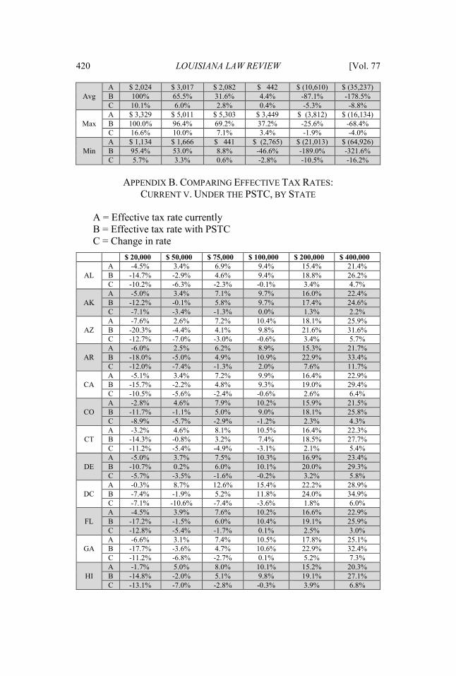
420 LOUISIANA LAW REVIEW [Vol. 77
Avg
A $ 2,024 $ 3,017 $ 2,082 $ 442 $ (10,610) $ (35,237) B 100% 65.5% 31.6% 4.4% -87.1% -178.5% C 10.1% 6.0% 2.8% 0.4% -5.3% -8.8%
Max
A $ 3,329 $ 5,011 $ 5,303 $ 3,449 $ (3,812) $ (16,134) B 100.0% 96.4% 69.2% 37.2% -25.6% -68.4% C 16.6% 10.0% 7.1% 3.4% -1.9% -4.0%
Min
A $ 1,134 $ 1,666 $ 441 $ (2,765) $ (21,013) $ (64,926) B 95.4% 53.0% 8.8% -46.6% -189.0% -321.6% C 5.7% 3.3% 0.6% -2.8% -10.5% -16.2%
APPENDIX B. COMPARING EFFECTIVE TAX RATES: CURRENT V. UNDER THE PSTC, BY STATE
A = Effective tax rate currently B = Effective tax rate with PSTC C = Change in rate
$ 20,000 $ 50,000 $ 75,000 $ 100,000 $ 200,000 $ 400,000
AL
A -4.5% 3.4% 6.9% 9.4% 15.4% 21.4% B -14.7% -2.9% 4.6% 9.4% 18.8% 26.2% C -10.2% -6.3% -2.3% -0.1% 3.4% 4.7%
AK
A -5.0% 3.4% 7.1% 9.7% 16.0% 22.4% B -12.2% -0.1% 5.8% 9.7% 17.4% 24.6% C -7.1% -3.4% -1.3% 0.0% 1.3% 2.2%
AZ
A -7.6% 2.6% 7.2% 10.4% 18.1% 25.9% B -20.3% -4.4% 4.1% 9.8% 21.6% 31.6% C -12.7% -7.0% -3.0% -0.6% 3.4% 5.7%
AR
A -6.0% 2.5% 6.2% 8.9% 15.3% 21.7% B -18.0% -5.0% 4.9% 10.9% 22.9% 33.4% C -12.0% -7.4% -1.3% 2.0% 7.6% 11.7%
CA
A -5.1% 3.4% 7.2% 9.9% 16.4% 22.9% B -15.7% -2.2% 4.8% 9.3% 19.0% 29.4% C -10.5% -5.6% -2.4% -0.6% 2.6% 6.4%
CO
A -2.8% 4.6% 7.9% 10.2% 15.9% 21.5% B -11.7% -1.1% 5.0% 9.0% 18.1% 25.8% C -8.9% -5.7% -2.9% -1.2% 2.3% 4.3%
CT
A -3.2% 4.6% 8.1% 10.5% 16.4% 22.3% B -14.3% -0.8% 3.2% 7.4% 18.5% 27.7% C -11.2% -5.4% -4.9% -3.1% 2.1% 5.4%
DE
A -5.0% 3.7% 7.5% 10.3% 16.9% 23.4% B -10.7% 0.2% 6.0% 10.1% 20.0% 29.3% C -5.7% -3.5% -1.6% -0.2% 3.2% 5.8%
DC
A -0.3% 8.7% 12.6% 15.4% 22.2% 28.9% B -7.4% -1.9% 5.2% 11.8% 24.0% 34.9% C -7.1% -10.6% -7.4% -3.6% 1.8% 6.0%
FL
A -4.5% 3.9% 7.6% 10.2% 16.6% 22.9% B -17.2% -1.5% 6.0% 10.4% 19.1% 25.9% C -12.8% -5.4% -1.7% 0.1% 2.5% 3.0%
GA
A -6.6% 3.1% 7.4% 10.5% 17.8% 25.1% B -17.7% -3.6% 4.7% 10.6% 22.9% 32.4% C -11.2% -6.8% -2.7% 0.1% 5.2% 7.3%
HI A -1.7% 5.0% 8.0% 10.1% 15.2% 20.3% B -14.8% -2.0% 5.1% 9.8% 19.1% 27.1% C -13.1% -7.0% -2.8% -0.3% 3.9% 6.8%

2016] GIVING CREDIT WHERE CREDIT IS DUE 421
ID
A -7.1% 1.9% 5.9% 8.7% 15.5% 22.4% B -15.3% -4.2% 3.1% 8.7% 21.7% 33.6% C -8.2% -6.1% -2.8% 0.0% 6.2% 11.2%
IL
A -4.0% 4.1% 7.7% 10.3% 16.5% 22.6% B -17.7% -3.0% 4.1% 8.9% 19.7% 28.1% C -13.7% -7.2% -3.6% -1.4% 3.2% 5.5%
IN
A -4.6% 3.7% 7.4% 10.0% 16.3% 22.7% B -16.9% -3.2% 4.9% 10.7% 21.9% 30.6% C -12.3% -6.9% -2.5% 0.6% 5.5% 7.9%
IA
A -5.2% 3.5% 7.4% 10.1% 16.7% 23.2% B -16.1% -3.5% 4.1% 9.6% 21.5% 31.3% C -10.9% -7.0% -3.2% -0.5% 4.8% 8.0%
KS
A -4.8% 3.5% 7.2% 9.8% 16.1% 22.4% B -15.0% -2.4% 4.9% 10.2% 21.5% 29.4% C -10.2% -5.9% -2.3% 0.4% 5.4% 7.0%
KY
A -4.9% 3.7% 7.5% 10.2% 16.7% 23.2% B -14.4% -3.2% 5.7% 11.4% 23.3% 32.8% C -9.5% -6.9% -1.8% 1.2% 6.6% 9.6%
LA
A -3.0% 4.2% 7.3% 9.6% 15.0% 20.4% B -13.6% -2.3% 4.0% 8.8% 18.0% 25.2% C -10.6% -6.5% -3.3% -0.8% 3.0% 4.9%
ME
A -1.8% 4.5% 7.2% 9.2% 13.9% 18.7% B -11.4% -0.8% 4.6% 8.5% 17.8% 25.9% C -9.6% -5.2% -2.6% -0.7% 3.8% 7.2%
MD
A -2.7% 4.7% 7.9% 10.3% 15.8% 21.4% B -12.4% -1.7% 3.7% 8.3% 18.2% 27.1% C -9.7% -6.4% -4.3% -2.0% 2.4% 5.7%
MA
A -2.1% 5.1% 8.2% 10.5% 15.8% 21.2% B -12.1% -1.5% 4.1% 7.9% 17.0% 24.9% C -10.0% -6.5% -4.1% -2.5% 1.2% 3.7%
MI A -4.8% 3.5% 7.2% 9.8% 16.1% 22.4% B -14.5% -3.0% 3.9% 9.1% 20.7% 30.2% C -9.7% -6.5% -3.3% -0.7% 4.6% 7.8%
MN
A -3.1% 4.4% 7.6% 10.0% 15.6% 21.2% B -11.9% -2.2% 3.8% 8.1% 19.1% 28.3% C -8.8% -6.5% -3.8% -1.9% 3.6% 7.2%
MS
A -4.6% 3.0% 6.3% 8.7% 14.3% 20.0% B -15.0% -4.6% 4.1% 9.3% 19.2% 27.9% C -10.4% -7.5% -2.2% 0.7% 4.9% 7.9%
MO
A -4.9% 3.6% 7.4% 10.0% 16.4% 22.8% B -14.4% -2.7% 4.1% 9.1% 20.2% 29.4% C -9.6% -6.3% -3.3% -0.9% 3.8% 6.6%
MT
A -1.9% 4.7% 7.6% 9.7% 14.6% 19.6% B -8.3% 1.3% 6.3% 9.8% 17.7% 25.0% C -6.4% -3.4% -1.4% 0.1% 3.1% 5.4%
NE
A -2.3% 4.5% 7.5% 9.6% 14.7% 19.8% B -13.1% -1.2% 5.5% 10.0% 19.4% 27.0% C -10.8% -5.7% -1.9% 0.4% 4.7% 7.2%
NV
A -5.1% 3.8% 7.7% 10.5% 17.2% 23.9% B -13.9% -0.9% 6.1% 10.6% 20.0% 27.4% C -8.7% -4.6% -1.6% 0.1% 2.8% 3.5%
NH
A -2.8% 4.2% 7.4% 9.6% 14.9% 20.3% B -11.5% -0.3% 5.1% 8.7% 16.6% 22.7% C -8.7% -4.5% -2.2% -0.9% 1.7% 2.4%

422 LOUISIANA LAW REVIEW [Vol. 77
NJ
A -5.1% 3.5% 7.3% 10.1% 16.6% 23.1% B -16.4% -3.4% 3.8% 8.2% 18.6% 28.5% C -11.3% -6.9% -3.6% -1.8% 2.0% 5.4%
NM
A -3.1% 4.0% 7.2% 9.4% 14.7% 20.1% B -13.5% -1.9% 4.2% 8.7% 18.2% 25.8% C -10.4% -6.0% -3.0% -0.7% 3.4% 5.7%
NY
A -4.6% 4.1% 7.9% 10.6% 17.2% 23.8% B -14.6% -4.7% 2.2% 7.8% 20.6% 32.9% C -10.0% -8.8% -5.7% -2.8% 3.4% 9.1%
NC
A -2.9% 4.0% 7.1% 9.3% 14.6% 19.9% B -12.6% -1.5% 4.7% 9.2% 19.1% 27.7% C -9.7% -5.6% -2.5% -0.1% 4.5% 7.9%
ND
A -2.5% 4.5% 7.6% 9.8% 15.1% 20.4% B -11.8% 0.2% 5.6% 9.2% 17.2% 23.8% C -9.3% -4.3% -2.0% -0.6% 2.2% 3.4%
OH
A -3.9% 3.9% 7.4% 9.8% 15.8% 21.7% B -15.4% -2.5% 4.8% 9.8% 20.8% 30.0% C -11.5% -6.4% -2.6% 0.0% 5.0% 8.3%
OK
A -4.7% 3.2% 6.6% 9.1% 15.0% 21.0% B -15.0% -3.4% 4.0% 8.9% 19.0% 27.1% C -10.3% -6.5% -2.6% -0.2% 3.9% 6.2%
OR
A -3.9% 3.9% 7.3% 9.7% 15.5% 21.4% B -12.2% -0.6% 5.2% 9.5% 19.8% 29.7% C -8.3% -4.5% -2.1% -0.2% 4.3% 8.3%
PA
A -2.2% 4.8% 7.8% 10.0% 15.3% 20.5% B -14.1% -1.0% 5.0% 9.3% 18.4% 25.1% C -11.9% -5.8% -2.8% -0.7% 3.1% 4.6%
RI A -3.1% 4.3% 7.6% 9.9% 15.5% 21.1% B -15.1% -2.1% 3.9% 8.6% 18.6% 27.4% C -12.0% -6.4% -3.6% -1.2% 3.1% 6.3%
SC
A -3.7% 4.0% 7.3% 9.7% 15.5% 21.3% B -10.8% -0.5% 5.5% 10.0% 20.7% 29.6% C -7.1% -4.4% -1.9% 0.3% 5.1% 8.3%
SD
A -2.8% 4.3% 7.4% 9.6% 15.0% 20.3% B -14.3% -0.3% 5.7% 9.5% 17.1% 22.9% C -11.5% -4.6% -1.7% -0.1% 2.1% 2.6%
TN
A -4.9% 3.5% 7.2% 9.8% 16.1% 22.4% B -15.9% -1.8% 6.6% 11.1% 19.6% 26.5% C -11.0% -5.3% -0.6% 1.3% 3.5% 4.0%
TX
A -7.5% 2.4% 6.8% 9.9% 17.4% 24.9% B -19.9% -4.1% 4.6% 10.1% 21.2% 29.8% C -12.3% -6.5% -2.2% 0.2% 3.8% 4.9%
UT
A -9.9% 0.5% 5.1% 8.4% 16.3% 24.2% B -19.4% -7.8% 1.6% 8.2% 22.9% 34.0% C -9.4% -8.3% -3.5% -0.2% 6.6% 9.9%
VT
A -1.8% 4.9% 7.9% 9.9% 15.0% 20.0% B -10.4% -1.7% 4.6% 9.6% 19.1% 28.1% C -8.7% -6.6% -3.2% -0.4% 4.1% 8.0%
VA
A -3.1% 4.8% 8.3% 10.8% 16.8% 22.8% B -11.8% -0.5% 5.0% 9.1% 19.0% 27.5% C -8.7% -5.3% -3.3% -1.7% 2.2% 4.7%
WA
A -3.4% 4.1% 7.4% 9.8% 15.4% 21.1% B -20.1% -2.7% 4.2% 8.5% 17.1% 23.6% C -16.6% -6.7% -3.2% -1.2% 1.6% 2.5%

2016] GIVING CREDIT WHERE CREDIT IS DUE 423
WV
A -6.5% 2.7% 6.8% 9.7% 16.7% 23.7% B -15.2% -4.0% 3.8% 9.6% 22.5% 33.8% C -8.7% -6.7% -3.0% -0.1% 5.9% 10.1%
WI A -4.5% 4.2% 8.0% 10.7% 17.3% 23.8% B -14.0% -3.3% 3.9% 9.3% 22.1% 32.7% C -9.6% -7.5% -4.1% -1.4% 4.8% 8.8%
WY
A -5.6% 3.4% 7.4% 10.2% 17.0% 23.8% B -13.8% -0.8% 6.0% 10.4% 19.1% 25.9% C -8.2% -4.2% -1.4% 0.2% 2.1% 2.1%
Max Current
Rate -0.3% 8.7% 12.6% 15.4% 22.2% 28.9%
Avg Current
Rate -4.2% 3.9% 7.4% 10.0% 16.0% 22.1%
Min Current
Rate -9.9% 0.5% 5.1% 8.4% 13.9% 18.7%
Max
PSTC Rate
-7.4% 1.3% 6.6% 11.8% 24.0% 34.9%
Avg Current
Rate -14.3% -2.2% 4.6% 9.4% 19.7% 28.4%
Min PSTC Rate
-20.3% -7.8% 1.6% 7.4% 16.6% 22.7%
Largest Change -16.6% -10.6% -7.4% -3.6% 7.6% 11.7%
Avg Change -10.1% -6.1% -2.8% -0.5% 3.7% 6.3%