Embed Size (px)
Citation preview

1
Faculty of Science and Technology
MASTER’S THESIS
Study program/ Specialization:
Petroleum Engineering/ Petroleum
Geosciences Engineering
Fall semester, 2012
Open
Writer:
Karina del R. Gil González
…………………………………………
(Writer’s signature)
Faculty supervisor: Dr Christopher Townsend
External supervisor(s): Dr Christopher Townsend
Title of thesis: 3D Geological Modelling of Kilve Beach SW England: normally faulted
Liassic limestones and shales.
Credits (ECTS): 30
Key words:
Normal Fault, Fault Zone, Major and Minor
Structures, Lower Liassic age.
Pages: 84
+ enclosure: 0…………
Stavanger, 02.01.2013

2
Abstract
This study is based on the outcrops examples on Kilve Beach area, which is the onshore
continuation of the Bristol Channel Basin, South of England, U.K. Kilve is a fault zone going
into Lower Jurassic age limestones and mudrocks. The faults are well exposed on the Limestone
bedding and related with the development of the Bristol Channel Basin during the Mesozoic
(Beach, 1989). None of the Faults described on this project have showed evidence of strike-slip
or reverse-reactivation that occurred in the Bristol Channel during the Tertiary (Beach, 1989).
The interpretation and understanding of the faults & horizons geometries are based on
measurements, photographs, maps and GPS data taken on the field.
The localities were divided in three (Kilve Pill, Major fault 1 (Syncline 1) and After Red House
or Major Fault 2 (Syncline 2)) in order to make a small scale interpretation due to the quality of
the exposure. Two master faults have been identified as Normal presenting E-W striking with dip
variable depending on the localities.
The three localities studied were dominated by E-W striking normal faults. The beddings exposed
on the beach and cliff section consist of limestone and organic-rich shale interbedded. In general
the dipping of these beddings was towards to the South-west.
The stratigraphic sequences and structural data were measured in the area and loaded in the
Petrel ™ software to build a 3D geological model. 18 faults were interpreted on the outcrops,
only 11 faults were included in the model (excluding the small reverse faults and those exposed
only in the cliff section). The results show a good matching between the faults and horizons in
the photographs digitized, also with the interpretations done in the field. The normal and reverse
faults and horizons presented the same behaviour as well as those which were interpreted
previously.
In addition, facies (i.e. sand and shale), petrophysical (i.e. porosity) and fluid properties (i.e.
water saturation) were generated to get the volume calculations.
The structural model built in this study, may be used to improve the understanding of the large
number of fields in the North Sea, which its developments are linked to the fault behaviour.

3
INDEX OF CONTENTS
1 Introduction ............................................................................................................................ 10
1.1 Study Area ................................................................................................................................. 11
1.2 Objectives .................................................................................................................................. 12
1.3 Previous works ........................................................................................................................... 12
2 Geological Context ................................................................................................................. 15
2.1 Outcrop Structural Review......................................................................................................... 17
2.2 Outcrop Stratigraphy Review ..................................................................................................... 17
3 Fault Description: Theory review .......................................................................................... 21
4 Measurements and Notation ................................................................................................... 24
5 Data Collection and field Observations ................................................................................. 26
5.1 Outcrop data ............................................................................................................................... 26
5.1.1 Locality 1 (Kilve Pill) .......................................................................................................................... 29
5.1.2 Locality 2 (2 Major Structural Elements –F5-Syncline1 and F12) ...................................................... 37
5.1.3 Locality 3 (F15- Syncline 2) ................................................................................................................ 42
6 Geological Modeling Process ................................................................................................ 48
6.1 Images Geo-referencing ............................................................................................................. 48
6.2 Surface reference data ................................................................................................................ 51
6.3 Structural Framework ................................................................................................................ 56
6.4 Fault diagnosis ........................................................................................................................... 58
6.5 Model Segmentation .................................................................................................................. 61
6.6 Zone Properties and Layering Process ....................................................................................... 64
6.7 Property Modeling ..................................................................................................................... 67
6.7.1 Geometrical Modeling .......................................................................................................................... 67
6.7.2 Facies Modelling .................................................................................................................................. 67

4
6.7.3 Petrophysical Modeling ........................................................................................................................ 69
6.7.4 Contacts and Volumens ........................................................................................................................ 69
7 Discussions ............................................................................................................................. 73
8 Conclusions ............................................................................................................................ 76
9 Recommendations for further work ........................................................................................ 77
10 References .............................................................................................................................. 78
10.1 Maps References ........................................................................................................................ 82
10.2 Manual references ...................................................................................................................... 82
11 Appendix ................................................................................................................................. 83
11.1 Raw data collected-GPS points .................................................................................................. 83
11.2 Fault data collected on the cliff section...................................................................................... 84

5
INDEX OF FIGURES
FIGURE 1.1 COMBINATION OF TOPOGRAPHIC MAP OF THE SOUTHWEST OF ENGLAND AND SATELLITE
IMAGE, SHOWING THE LOCATION OF KILVE BEACH AND THE THREE LOCALITIES WHERE THE
FIELDWORK WAS CARRIED OUT. BASED ON A SMALL PART OF ORDNANCE SURVEY FROM ANQUET
MAPS 2011, ORIGINALLY 1:25,000 SCALES. ............................................................................... 14
FIGURE 2.1 STRATIGRAPHIC CORRELATION OF THE LOWER LIASSIC EXPOSURE AT KILVE BEACH,
COMPARED TO PUBLISHED ACCOUNTS (MODIFIED BY BRODAHL, E. (1993) AND KELLY ET AL,
1998) ....................................................................................................................................... 18
FIGURE 2.2 OUTCROP AND SUBCROP LIAS GROUP IN ENGLAND AND WALES SHOWING THE KILVE
LOCATION AND MAIN SEDIMENTARY BASIN. AFTER COX ET AL. (1999) AND SIMMS ET AL.(2004) .. 19
FIGURE 2.3 MAJOR GEOLOGICAL FEATURES OF SOUTH WALES AND THE BRISTOL CHANNEL BASED ON
BRITISH GEOLOGICAL SURVEY MAPS AND TAPPIN ET AL. (1994). A = VARISCAN FRONT THRUST, B
= CENTRAL BRISTOL CHANNEL FAULT ZONE. ............................................................................ 20
FIGURE 3.1 EXAMPLE OF NORMAL FAULT WITH ITS DIMENSIONS ........................................................ 21
FIGURE 3.2 FIELD EXAMPLE SHOWING MAYOR AND MINOR STRUCTURES. ............................................ 23
FIGURE 4.1 TOOLS USED IN THE MEASUREMENTS AND NOTATION ....................................................... 25
FIGURE 5.1 A) PROFILE ON THE CLIFF AND B) THE BEACH EXPOSURE, FAULTS INTERPRETED (2 MAJOR
FAULTS (IN RED), INTO THE MINORS FAULTS ARE 2-REVERSE FAULTS (IN WHITE) AND 9 NORMAL
FAULTS (IN YELLOW)) ................................................................................................................ 28
FIGURE 5.2 FAULT 1 OVERVIEW ON THE LOCALITY 1 .......................................................................... 29
FIGURE 5.3 MEASUREMENTS ON THE CLIFF SECTION -LOCALITY 1 ..................................................... 32
FIGURE 5.4 NORMAL FAULTS F1 AND F2A SEEN ON THE CLIFF SECTION. ............................................ 33
FIGURE 5.5 ZOOM ON THE NORMAL FAULT F4. .................................................................................. 34

6
FIGURE 5.6 A) LOCALITY 1 CLIFF SECTION AND BEACH EXPOSURE- F1 &F2AND B) EXAMINATION IN
THE STRIKE, DIP AND THICKNESS DIMENSION DUE TO THE PRESENCE OF A CAVE AND IN THE LOWER
PART OF THE HANGING WALL GOOD EXPOSURE THE FAULT CORE SEGMENTED ............................. 36
FIGURE 5.7 LOCALITY 2-A) FAULT INTERPRETATIONS ON THE BEACH MNF (F5) AND OTHERS FAULTS, B)
THE SYNCLINE 1 SEEN FROM THE CLIFF, C) NORMAL FAULTS RELATED TO THE MNF (F5). ........ 38
FIGURE 5.8 OVERVIEW BETWEEN F7 & F8 INTERPRETATION ON THE CLIFF ........................................ 40
FIGURE 5.9 OVERVIEW BETWEEN F12 INTERPRETATION ON THE CLIFF ............................................... 41
FIGURE 5.10 RELAY RAMP SEEN IN THE LOCALITY 3 AND DIAGRAM TAKEN IN ACCOUNT IN THE
INTERPRETATION. ..................................................................................................................... 44
FIGURE 5.11 TO 1.3 KM EAST TO KILVE PILL, DIRECTION LILSTOCK, DOMES STRUCTURES AND
AMMONITES. ............................................................................................................................ 45
FIGURE 5.13 LOCALITY 3: FAULTS INTERPRETATION ON THE BEACH AND CLIFF SECTION; ONLY 3 FAULTS
WERE INTEGRATED IN THE 3D GEOLOGICAL MODEL.(F13, F14 AND F15). ................................. 47
FIGURE 6.1 GEOREFRENCING PROCESS OVERVIEW. ........................................................................... 49
FIGURE 6.2 OVERVIEW THE GEO-REFERENCING INTO PETREL ............................................................ 50
FIGURE 6.3 SCHEME SHOWING THE INPUT DATA FILTERED IN ORDER TO GENERATED THE HORIZONS AND
FAULT SURFACE ........................................................................................................................ 51
FIGURE 6.4 MAPPING WORKFLOW USED ............................................................................................ 52
FIGURE 6.5 PETREL OVERVIEW OF THE LAYER AND FAULT SURFACE PROCEDURE ................................ 53
FIGURE 6.6 MAKE SURFACE PROCESS ............................................................................................... 54
FIGURE 6.7 OVERVIEW ISOCHORS SURFACES PROCESS BY BLOCK ....................................................... 55
FIGURE 6.8 FAULT MODELLING PROCESS ......................................................................................... 56
FIGURE 6.7 FAULT MODELLING PROCESS: FAULTS (SURFACES AND PILLARS), CONNECTION AND
CONSISTENCY BETWEEN THEM ................................................................................................... 57
FIGURE 6.10 PILLAR GRIDDING PROCESS .......................................................................................... 58

7
FIGURE 6.11 PILLAR GRIDDING PROCESS: SKELETON GRID GENERATION BASE ON THE KEY PILLAR
DEFINED IN THE PREVIOUS PROCESS. ......................................................................................... 59
FIGURE 6.12 FAULT INTERPRETATIONS: GOOD COMPARISON BETWEEN FIELDWORK AND PETREL.
(CHECKING THE GOD MATCHING) ............................................................................................. 60
FIGURE 6.13 MAKE HORIZON PROCESS ............................................................................................. 61
FIGURE 6.14 MAKE HORIZONS PROCESS INCLUDES INTERPRETED HORIZONS AND QC IN THE
STRATIGRAPHY SHOW IN 3D BY INTERSECTION (GRID I-DIRECTION). ........................................... 62
FIGURE 6.15 MAKE HORIZON PROCESS: OVERVIEW OF SEGMENTATION ( DONE BY BLOCKS). .............. 63
FIGURE 6.16MAKE ZONES PROCESS SHOWING FROM TOP-L8 AND TOP-L19 INSERTED GEOLOGICAL
ZONES IN THE STRATIGRAPHIC INTERVALS. ................................................................................. 66
FIGURE 6.17 PROPERTY MODELING SCHEME .................................................................................... 67
TABLE 6.1 VARIOGRAM SETTING FOR THE SAND FACIES. .................................................................... 68
FIGURE 6.18 QC THE FACIES MODELS GENERATED............................................................................ 68
FIGURE 6.19 GEOMETRICAL MODELLING SHOWING IN 3D VIEW: CONNECTED VOLUME AND FACIES
PROPERTY GENERATED.............................................................................................................. 70
FIGURE 6.20 PETROPHYSICAL AND FLUID PROPERTIES ...................................................................... 71
FIGURE 6.21VOLUME RESULTS ......................................................................................................... 72

8
INDEX OF TABLES
TABLE 2.1 DISCRETE PHASES ______________________________________________________ 15
TABLE 5.1 COMPARISON OF THE DIPS OF THE SOUTH-DIPPING AND NORTH-DIPPING NORMAL AND
REVERSE FAULTS ___________________________________________________________ 39
TABLE 6.1 VARIOGRAM SETTING FOR THE SAND FACIES. __________________________________ 68
TABLE 11.1 GPS POINTS COLLECTED IN THE AREA ACCORDING TO THE FAULT BLOCK ____________ 83
TABLE 11.2 DIP AND STRIKE VALUES TAKEN IN THE CLIFF SECTION __________________________ 84

9
Acknowledgments
This project of the Master Thesis has been performed with the Department of Petroleum
Engineering, University of Stavanger (UiS), Norway, in cooperation with Total E&P Norge AS
during fall term 2012.
It was supervised by Dr. Christopher Townsend whom I would like to convey sincere Thanks for
his supervise and support on this project, adding enjoyable discussions on the field and useful tips
regarding Petrel Software that served in enriching my knowledge.
I am really grateful with the Department of Petroleum Engineering, University of Stavanger for
giving me the financial support on the field trip that was the occasion of fruitful exchanges
between the field experience in addition with the interpretation of the structures seen and finally
to build a proper 3D model of the area in study of my master thesis.
A Special Thanks to Lisa Bingham for her assistance in ArcGis tool and to Dr Alejandro
Escalona for giving the opportunity be part/student of the Petroleum Geosciences specialization
and provide to me the solid knowledge in sedimentation and key ideas in subsurface
interpretation.
I would like to thanks to my husband, Freddy Oliveira for his patience, support, useful
suggestions and critical remarks through the text. In Addition, I am very grateful with my God,
family and friends who with enthusiasm and continue support helped me developing my thesis
project.

10
1 Introduction
The trapping, the hydrocarbons’ migration, and the evolution of the basins come from the normal
faults systems. Recent works (Walsh et al; 1991) have demonstrated the evolution and
geometries in well exposed areas, which provide a guide for the interpretation of the larger fault
zones, as well as understanding the formation of oil and gas fields.
In addition to describing fault style and fault mechanism, much has been published in recent
literature about the applicability technique to extensional basins. (Freeman et al, 1990)
The Faults and horizons geometries have been mapped from Lower Jurassic sequences on the
cliff sections, and a well exposed wave-cut platform on Kilve Beach which lies on the south side
of the Bristol Channel, England; UK.
The Kilve Beach area has been interpreted as normal fault system; their geometry and evolution
play an important role for hydrocarbon reservoirs because oil and/or gas are frequently trapped in
normal fault systems. Detailed studies of faulted outcrops help the understanding and
interpretation of seismic data as they provide real geometrical examples to hang interpretations
on. Additionally, they contribute in the understanding of how geological structures trap oil and
gas. The Kilve Beach area was the influenced by faults and linkage between each other.
Strike and dip measurements were taken on the fault surfaces and limentones beds, adding to the
last ones, thickness measurements. The beds correlations were generated according to the
stratigraphic column in the cliff section generated by Brodahl, E. (1993), and for the tidal
exposure that mapped by Kelly et al., 1998. The area is still subject to multiple interpretations
and studies due to the complexity in the structures present on the outcrops.
The field data have been used to construct a 3D structural-stratigraphic model (into a 3D
geological reservoir model) using the Petrel 3D modeling software.
A difference between this study and the previous studies (e.g. Brodhal 1985 and Øyvin 1995) is
that the field data collected from the outcrops was interpreted to support a 3D geological model
building of the area.

11
The detailed level in 3D geological modeling was constrained by the input and process time of
the data (representing the horizon and faults as they were seen on the field).
1.1 Study Area
This study is based on outcrops examples from Kilve Beach area, which are situated on the
southern of Bristol Channel basin, England. The Bristol Channel Basin belongs to a series of
Mesozoic extensional grabens between Wales and Somerset (Lindanger, et al 2007). This Area is
localised about 2 km from the centre of Kilve’s town (Figure 1.1). The study area is characterised
by Normal Faulting with fold geometries. From previous work realised (Brodahl, 1993) the rocks
exposed on the Tidal platform and in the cliffs belong to the Lower Liassic age (Lower Jurassic).
The Fault zones have been described in small-scale at Kilve going into Lower Jurassic Limestone
and mudrocks age (the grid references ST314-144-145 and ST315-144-145 shown on the
Ordnance survey-Quantock Hills and Bridgwater-1:25000 scale) (Figure 1.2). These faults are
well exposed on the Limestone bedding and related with the development of the Bristol Channel
Basin during the Mesozoic (Beach, 1989). According to Beach (1989), one of the fault showes
evidence of strike-slip or reverse-reactivation that occurred in the Bristol Channel during the
Tertiary. As mentioned above, the beddings exposed in the beach consists of limestone benches,
whereas on the cliffs, these are formed by organic-rich shale interbedded with argillaceous
limestone. The area is dominated by E-W striking normal faults, and small reverse movements
identified on the Fault planes. The dip dimensions have been taken on the field over the faults
and beddings (in the cliffs and the beach surface respectively).
The Field interpretation was done based on the maps (from the Ordnance survey-Quantock Hills
and Bridgwater maps -1:25000 scale), Photographs (taken on the Field), satellite images
(digitized from Anquet map 2011software in combination with those given by Google earth) GPS
measurements points. The data and interpretation were used to build the 3D geological Model in
Petrel.
These localities have been mentioned above by Elizabeth Brodahl in 1993, Steen Øyvind in 1995,
and other researchers. The fieldwork was carried out in three locations (location 1-Kilve Pill,
location 2- starts in F5 identified as major fault 1 (overview of syncline 1) - and location 3- starts

12
in F13 (overview of syncline 2)-). This area represents approximately 1, 5 Km from Kilve Pill to
the east part direction Lilstock, where the beach is facing towards the north. (Figure 1.3)
1.2 Objectives
The purpose of this study is to describe the behavior of the faults and horizons on the Kilve
Beach outcrops (a faulted area with Liassic limestone and shale beds), in the Southwest of
England by using field work data collection and the construction of 3D structural model of the
area. (Figure 1.4)
The field work objectives included the mapping of the key horizons and structural elements
(faults), using detailed stratigraphic correlation
The structures were mapped by making outcrops observations and the acquisition of relevant
field data using GPS measurements, as well as air photos and satellite images.
Finally, a 3D model of the fault blocks interpreted was built by using Petrel ™ software. This
model may be used as an analogue for oil and gas fields.
1.3 Previous works
Most of the references on this study come from previous data, taken in the Kilve Outcrops studies
which are unpublished Msc theses (such as Brodahl, E. 1993 and Steen, Ø. 1995). These studies
presented detailed stratigraphic correlations, and field observations using dip meter logs which
were used to recognize in small and big scale, the main structures and major faults of the area.
Brodahl, E. (1993), mapped the structures location which extends around 6 km along the Kilve
Beach. The cliff exposures projections were taken by measuring the length, displacements,
thickness, lithology and the fault planes. She claimed that the Kilve location was dominated by a
fractal extensional deformation where the main faults were normal faults, including the antithetic
faults found in the East of Bristol Channel Basin. In addition, she documented a detailed profile
of the cliff, and showed a map of stratigraphic framework of the sections helped with
photographs, which were taken during the fieldwork in combination with the aerial photographs
from the territory

13
Steen, Ø. (1995), tested the reliability of fault interpretations by studying the geometry of the
faults and their associated fold outcrops of Kilve Beach. The deformation related to normal faults
in Kilve include normal drags fold, reverse drag folds and roll-over anticlines above listric faults.
Steen claimed that the width and accentuation of normal drags folds in Kilve tend to saturate for
faults displacement from 10 m up to 60 m.
The tectonic influence on deposition and stratigraphy framework was described by Tankard et. al
(1989),who included the Bristol Channel as part of Celtic Sea Basin and claimed that it had been
subjected to three discrete phases of extension and fault controlled subsidence, each phase was
followed by a period of thermally controlled passive subsidence. The outcrops studied belong to
Lias, which has extensive subcrop in England. Their thick successions have been proven by
boreholes in the North Sea, Hebrides Sea, Irish Sea, Bristol Channel and Cardigan Bay (Simms et
al., 2004). Moreover, the Lower Lias stratigraphy was used from the Palmer’s interpretation in
1972 and Whittaker and Green, (1983), followed in detail by Brodahl, E., (1993). That was
treated in combination with Peacock’s paper (1998) about the tectonic evolution of the Bristol
Channel Basin, the linkage and interaction in normal fault systems, has been taken into account to
understand the geometries and evolution of Normal Faults in the Jurassic sedimentary rocks of
the Somerset coast.
A study from Peacock and Sanderson (1994) interpreted the relay ramp in the east of Kilve Pill.
They described the relay ramp as open and continuous structure that maintains the continuity
between the footwall and hanging wall. In suitable outcrops, fault tips involved in the relay ramp
can be observed directly, whereas in seismic data there is an inherent resolution limit below
which discrete fault geometries cannot be imaged (Townsend et al., 1998).
Conford (2003), interpreted the presence of domes structures to 1.3 km east to Kilve Pill in the
direction Lilstock. The domes structures were uplifted in the carbonate and were prominent as a
result of erosion overlying mudstones unit. In addition, these structures were shown in the
hanging wall of the relay ramp interpreted by Peacock and Sanderson (1994).

14
Figure 1.1 Combination of Topographic Map of the Southwest of England and satellite image, showing the location of Kilve Beach and the three localities where the fieldwork
was carried out. Based on a small part of Ordnance Survey from Anquet maps 2011, originally 1:25,000 scales.

15
2 Geological Context
The study area is located in the Kilve Beach, southern margin of the eastern branch in the Bristol
Channel Basin (Figure 2.1 and 2.2). It belongs to the Mesozoic Grabens in southern England
(Glen & Whittaker, 2005) and Celtic Sea basins (Figure 2.2). The area is of a normal fault series
outcrops. The basin has been subject to three discrete phases of extension and fault controlled
subsidence which could be recognized, each phase was followed by a period of thermally
controlled passive subsidence (Tankard et. al 1989) as shown below:
Table 2.1 Discrete phases
Phase Extension Passive Subsidence
1 Permian to Triassic (Synrift I) Hettagian to Oxfordian
2 Late Jurassic (Synrift II) Tithonian to Berriassian
3 Early Cretaceous (Synrift III) Aptian to Maestrichtian
The first phase, Synrift (I) is a series of northeast-southwest trending controlled by small faults,
and isolated basins probably developed in the Late Permian (Van Hoorn 1987). The facies
development in the axis of Bristol Channel basin were dominated by evaporitic mudstones,
grading upward into massive halite and later on, these mudstones grade upward into a restricted
marine latest Triassic sequence of anhydritic mudstones, sandstones and limestones, reflecting
the start of the major marine transgression.
The first passive subsidence was associated with a combination of local variations in subsidence
rates, and more widespread changes in sea level (Millson 1987). The deposition during this
period was characterized by a series of regressive-transgressive cycles, within a gently subsiding
basin. It started in the Hettagian with an initial regression, followed quickly by a transgression in
the Late Triassic, resulting in dominant mudstone facies and thin cycles of micritic limestone.
Just before the Sinemurian, a basin wide transgression started characterized for open-marine

16
conditions where the sedimentation process was dominated by mudstone and thin limestones. The
late Oxfordian was assigned as unconformity (Millson 1987).
The Synrift (II) was the result of the faults reactivation controlled by subsidence in the pre-
existing Triassic rift basins, and initiation of further basins (Masson and Miles 1986a). The
structural response, uplift and erosion were associated with an extensional episode where the
Bristol Channel basin was actively subsiding. Fluvio-lacustrine and lagoonal to marginal-marine
facies were developed.
In the second passive subsidence, it was active extension and fault controlled subsidence
continued, which was associated with substantial uplift of the basins ended. The marine influence
over the interbedded coarse clastic and limestone was developed (Tankard et. al 1989).
The Synrift (III) phase is a series of northeast-to-southwest and east-west trending extensional
faults, which were reactivated in a translational sense in the Celtic Sea basins (Van Hoorn 1987).
One of the Celtic Sea Basins, The Bristol Channel basin, was dominated by transgressions
through the Early Cretaceous. The facies were developed in a marine transgression.
During the third passive subsidence, uplift resulted from local changes in subsidence rates and
possible regional changes in sea level. Transgressive clastic facies units were developed (Tankard
et. al 1989).
The local structural Framework was given by extensional faults behavior, exposed on the
outcrops. These outcrops belong to the Lower Jurassic series in Britain, and unbroken strips of
different thickness, extending from East Devon and West Dorset Coast, north-northeast through
Somerset, Gloucestershire, the east Midlands and Humberside, in the coast of Cleveland and
North Yorkshire (Simms et al., 2004).
The Eastern of the Kilve Area (locality 3, Figure 4.XX) is characterised of the Early Lias
formations (started in the Triassic) with several metres of beds above the Penarth Group, and
identified as younger formation. From here it runs through the Hettangian Stage of the Lower
Jurassic, and into the Semicostatum Zone of the Sinemurian Stage, where the cycles of limestone
and shale gradually change into the predominantly mudstone. In addition, a variety of fossils

17
record is preserved on beds in the Kilve area. Additionally, the large ammonites were found in
the area, which is visited by several research groups due to the fantastic exposures and easy
access to the beach.
2.1 Outcrop Structural Review
The outcrops studied belong to the Lias, which has extensive sub-crop in England (Figure 2.2). A
series of investigation of both onshore and offshore outcrops/sub-crop by drilling and
geophysical methods, in association with hydrocarbon exploration, has revealed the nature, extent
and structure of Lower Jurassic in Britain. Their thick successions have been proven by boreholes
in the North Sea, Hebrides Sea, Irish Sea, Bristol Channel and Cardigan Bay (Simms et al., 2004).
2.2 Outcrop Stratigraphy Review
The lower Jurassic rocks of Great Britain are predominantly marine mudstones that have been
grouped together under the name “Lias” since the early part of the 19th
century. They form a
distinctive succession of marine carbonates where the Lias was deposited in a series of
interconnected sedimentary basins and shelf areas, producing local differences in the sedimentary
successions (Simms et al., 2004). Nonetheless the local successions were correlated, and some
stratigraphic levels have been recognized across the largest outcrops studied in Kilve Beach.
Stratigraphic framework of the Lower Lias for the cliff section used in this study was mapped by
Brodahl, E. (1993) ( the measurements were taken in 109 beds in the cliff at the west of Lilstock
and 39 beds on the foreshore east of Kilve) , following the Palmer (1972) and interpretation and
Whittaker and Green, (1983), where the sequences were correlated to the biostratigraphy;
combining with that mapped by Kelly et al, (1998) on the foreshore taking in account the
stratigraphy generated by Whittaker and Green, (1983) in order to generate a good correlation
between outcrops. In addition, the resolution of the images allowed accurate placement of the
stratigraphic boundaries. (Figure 2.1).

18
LO
WE
R J
UR
AS
SIC
Lo
wer
Lia
s
Het
tan
gia
nS
inem
uri
an
AgeBed no of base and
Divisions (Thickness)
257+
Division 5 (80 m)
204
203
Division 4 (40 m)
147
146
Division 3 (50 m)
69
68
Division 2 (20 m)40
1-39 Division 1 (13 m)
Whittaker & Green (1983)
Aldergrove Beds
St. Audries
Shales
Blue Lias
Kilve Shales
Quantock’s Beds
Doniford Shales
Helwell Marls
PALMER (1972)
Brodahl, E. (1993).
Quantock’sBeds
( From L3 to LA)
0 m
50 m
100 m
150 m
Kilve Shales
( From base L7 to top L4)
Blue Lias
(From Base
L25 to L7)
St. Audries
Shales
+ L25
Doniford Shales
(LB1-LA1)
This Study
Divisions
Early Lias
Divisions
Figure 2.1 Stratigraphic correlation of the Lower Liassic exposure at Kilve Beach, compared to
published accounts (modified by Brodahl, E. (1993) and Kelly et al, 1998)

19
Figure 2.2 Outcrop and subcrop Lias Group in England and Wales showing the Kilve location and main sedimentary basin. After Cox
et al. (1999) and Simms et al.(2004)

20
Figure 2.3 Major geological features of South Wales and the Bristol Channel based on British Geological Survey maps and Tappin et
al. (1994). A = Variscan Front Thrust, B = Central Bristol Channel Fault Zone.

21
3 Fault Description: Theory review
For the geoscientist, it is important to get an overview about the structural geology concerning
the faults analysis. A fault can be transmitter or barrier to fluid flow and pressure communication.
The understanding of the fault behavior is fundamental for hydrocarbon fields drilling,
exploration and development.
According to the data collected in the field, analysing the major structures (dominated by normal
faulting), and recent works developed in Kilve Beach area, the area is presented as an extensional
settings. The small reverse faults interpreted on the outcrops will be shown as overview but not
described in detail.
Key definitions and drawings are shown in order to explain different components that should be
taken in account in fault analysis.
Foot Wall
Hanging Wall
121
2
Displacement
Throw
Heave
Fault Plane
Figure 3.1 Example of Normal fault with its dimensions
Fault zone: a zone containing a number of sub-parallel or anastomosing fault surfaces.
Fault: a surface along which appreciable displacement has taken place; this surface may be
planar or curviplanar (listric).

22
Footwall: the body of rock immediately below a non-vertical fault. The body of rock itself is
called the footwall block.
Hanging wall:the body of rock immediately above a non-vertical fault. The body of rock itself is
called the hanging wall block.
Throw: vertical component of fault displacement.
Heave: horizontal component of fault displacement.
Fault displacement: The offset of segments or points those were once continuous or adjacent.
Rocks beds that have been moved by the action of faults showing displacement on either side of
fault surface.
Extensional Fault: a fault which produces horizontal lengthening as measured across the trace of
the fault.
In the study area, it was identified two major structures and minor structures associated which
help in the evolution of the normal faulting. These played an important role in the faults
correlation minimizing the risk in the regional context. Figure 3.2 shows these structures on the
cliff.
Major Structure: is the largest observed size (fault with most important throw, largest structure)
Minor structure: is the lower size compared to major one and/or which development is directly
related to the major structure.

23
SWNE Locality 2: Major and minors Structures
Direction
Lilstock
Layer 7
1 m
Kilve Shale Formation
Kilve Shale Formation Blue Lias Formation
F8
F7
F11
76
65 89
47 45 42
52
a) Cross section of a fault with 2-hard linked
splays as show in the Major Normal Fault-
F12 and b) Block diagram showing the
geometry in 3D
Figure 3.2 Field example showing mayor and minor structures.

24
4 Measurements and Notation
The devices used consist of a ruler, measuring tape (10 m), GPS (Garmin-using Waypoints
indicating the latitude and longitude coordinates even in degree or cardinal letters (N,S,E,W),
the accuracy of this device is <10 m (33 feet) 95% typically), Compass Burton and Camera
(with a small tripod).
Fault displacements were measured using the ruler and the measuring tape (the errors are
subject to the irregular nature of the bedding planes)
The faults interpretation and mapping were produced using photographs taken in situ and
maps from Anquet maps (a program commercially available on the Ordenance Survey in UK)
helped with the Google Earth photos as base maps. In order to have good resolution and
vision in different angles of the land exposures, the photos were taken from the top of cliffs to
visualize the tidal platform and around 5m from the beach exposure to show the cliff sections.
On the faults, it was measured the strike-dip (using compass brunton), the limestone bedding
planes related to these with the bed height measurement respectively.

25
A&B) strike /Dip measurements and
interpretation according to the bed plane
C
C. – Acquisition of GPS points and D.- Measuring tape of 10 m.
D
Figure 4.1 Tools used in the measurements and notation

26
5 Data Collection and field Observations
The fault zones (to be described later on this report), are located on the Onshore-Lower Jurassic
limestone and shale at Kilve Beach in Bristol Channel, South of England. The faults were well
exposed on the cliffs (up to 40 m high) and on the tidal flat (up to 500 meter wide) (Øyvind,
1995).
The Kilve Beach is facing towards the north and the E-W oriented Bristol Channel Basin. The
area is dominated by normal faults probably related to a series of events occurred in the Bristol
Channel basin during the late Jurassic- Early Cretaceous.
5.1 Outcrop data
The layers’ surfaces on Kilve Beach outcrops were continue on the cliff, and around 80%-90% of
exposure on the beach, most of them were parallel to each other (sandstone-shale-sandstone) and
very distinctive. The sandstone surfaces were easy to recognize and be followed across the
outcrops and faults.
The thicknesses were measured using measuring tape. For those cases where the thickness was
not exposed, the strike and dip values were estimated. The length of some faults accessible, and
well exposed were also measured. The dip and strike measurements were taken with a compass
on the beddings and fault surfaces.
The major sedimentary and structural elements in the outcrop were identified. All faults and
beddings were mapped at a scale of 1:25000, both in plane and profile/cross-section. These
beddings were inside an extensional system composed by several normal faults where 14 of them
were identified as normal where 2 were selected as major normal faults due to the length
dimension and several branches (both identified on the locality 2) and 4 small reverse (Figure
5.1). These were also named as MNF1 (F5 in Figure 5.8) is related to the Syncline 1 and MNF2
(F12 in Figure 5.9) respectively.
27
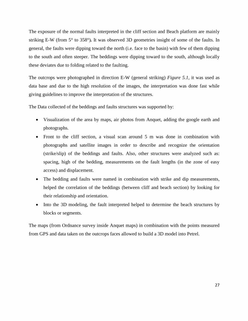
The exposure of the normal faults interpreted in the cliff section and Beach platform are mainly
striking E-W (from 5° to 358°). It was observed 3D geometries insight of some of the faults. In
general, the faults were dipping toward the north (i.e. face to the basin) with few of them dipping
to the south and often steeper. The beddings were dipping toward to the south, although locally
these deviates due to folding related to the faulting.
The outcrops were photographed in direction E-W (general striking) Figure 5.1, it was used as
data base and due to the high resolution of the images, the interpretation was done fast while
giving guidelines to improve the interpretation of the structures.
The Data collected of the beddings and faults structures was supported by:
Visualization of the area by maps, air photos from Anquet, adding the google earth and
photographs.
Front to the cliff section, a visual scan around 5 m was done in combination with
photographs and satellite images in order to describe and recognize the orientation
(strike/slip) of the beddings and faults. Also, other structures were analyzed such as:
spacing, high of the bedding, measurements on the fault lengths (in the zone of easy
access) and displacement.
The bedding and faults were named in combination with strike and dip measurements,
helped the correlation of the beddings (between cliff and beach section) by looking for
their relationship and orientation.
Into the 3D modeling, the fault interpreted helped to determine the beach structures by
blocks or segments.
The maps (from Ordnance survey inside Anquet maps) in combination with the points measured
from GPS and data taken on the outcrops faces allowed to build a 3D model into Petrel.

28
Locality 1 (Kilve Pill)
Locality 2Start Point F5
Locality 3Start Point F13
E Wa)
Beach Level
F1
F4
F7
F8
F9F10
F10-AF11
RED HOUSETop of the cliff
F7
4
1111
F5
b)
RELAY RAMP
N
Loc 1Loc 2
Loc 3
Dome structures
F13
F1F2A
F3-RF
& F4
F14
F15
F8 F7F10-RF
F11
F9 F2-RF
Syncline 1
Syncline 2
12
4
77
Kilve Shale
Formation
Blue Lias
Formation
Layer 7- limestone bed Layer 1 - limestone bed Layer 11- limestone bed
Quantock’s
Beds
St. Audries
Shales
Figure 5.1 a) Profile on the Cliff and b) the Beach exposure, Faults interpreted (2 major Faults (in red), into the minors faults are 2-reverse faults
(in white) and 9 normal faults (in yellow))

29
5.1.1 Locality 1 (Kilve Pill)
It is the coastal path along the northern flanks of the Quantock hills. This section is characterised
by an excellent outcrop exposed on the cliff (Figure 5.2), which is pointing to the North showing
a normal fault (Identified as the Major fault) where the bedding/rocks above the fault surface
have slipped down-wards and the limestone bands in the cliff foot have been faulted down about
3, 5 m, below the beach level in the block forming the head land. The fault is striking N15°W
presenting a dip of 45° towards to the North.
3
2
F1
11
23
4
E W
9
10
88
015/45
Figure 5.2 Fault 1 overview on the locality 1

30
5.1.1.1 Locality 1 Layers Description
On the first Cliff section, six layer (limestone beds) were identified as oldest deposition, from
layer 6 on the base of the cliff and layer A on the top of the cliff following the stratigraphic
sequences generated by Brodahl, E. (1993) and the author interpretations (Figure 5.3). The
youngest ones in place are in the eastern part of the area, near to the last study location (locality
3). (Figure 5.4)
The limestone beds shows on the cliff have been correlated across the faults (F1 and F2 defined
as the big ones). Some Normal drags structures on the footwall and hanging wall shown that
effectively it was a normal fault. Towards the eastern of the cliff, there are indicators of small
reverse movements (Figure 5.4). But these are not shown in the west side of the cliff studied on
this location 1. In general, the rocks associated to the fault and interbedded shale with limestone
benches.
On the cliff section, the thickness of limestone beds in the hanging wall varies between 15 cm
and 35cm while in the footwall varies between 22 cm to 44 cm, for the shale beds it could vary
between 43 cm to 1.2 m (Figure 5.5). The dipping of these layers is towards to the south-west
with an average of 19° in the footwall and 13° in the hanging wall .
The fault (F1) damage zone was around 80 cm thick in the footwall and 1.2 m in the hanging wall
observed as small tension fractures varying in orientation east-west most of them without any
measurement in displacement. In the fault plane was observed a thin fault core with a small
thickness around 6 cm in the upper part (up the limestone layer 1) and the lower part (near to the
beach level) and around 60 cm in the middle part (close to the limestone layer 1 and 2); in
addition, the fault core consists of predominant limestone and the thickest shale fabric parallel to
the fault surface.
On the beach, there was a well exposure of which block is the footwall and hanging wall, also a
good orientation of the fault surface and beds which basically present the same type of rock
shown on the cliff. (Figure 5.6, 5.5 and 5.6)
On the beach exposures, the thickness of limestone beds (marked as numbers on the section) in
the footwall are between 14 cm to 50 cm, in the hanging wall varies between 20 cm and 40 cm,
and for the shale beds it could vary between 17 cm to 3 m. The dipping of these layers are

31
towards to the south-west with an average of 13° in the footwall and 10° in the hanging wall, also
no significant rotation anticlockwise during the faulting. (Figure 5.5)
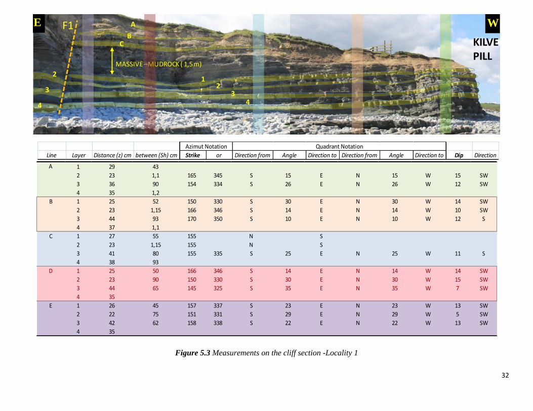
After the second fault (F2A) seen in the cliff, a long cliff section with parallel layers were
observed where three thick limestone layers were identified close to the beach level separating
with a massive mud rock around 2 m the youngest layers (identified as A,B and C respectively)
and later on those disappear. (Figure 5.1)
On the beach section a third fault was interpreted named F3, start in the layer 6 and die out on
the fault F2, the layers are also parallel showing a dip average of 10 ° toward to the south and
N84W then it was linked with the F4 and the end of the long cliff section. (Figure 5.4)
32
Line Layer Distance (z) cm between (Sh) cm Strike or Direction from Angle Direction to Direction from Angle Direction to Dip Direction
Azimut Notation Quadrant Notation
A 1 29 43
2 23 1,1 165 345 S 15 E N 15 W 15 SW
3 36 90 154 334 S 26 E N 26 W 12 SW
4 35 1,2
B 1 25 52 150 330 S 30 E N 30 W 14 SW
2 23 1,15 166 346 S 14 E N 14 W 10 SW
3 44 93 170 350 S 10 E N 10 W 12 S
4 37 1,1
C 1 27 55 155 N S
2 23 1,15 155 N S
3 41 80 155 335 S 25 E N 25 W 11 S
4 38 93
D 1 25 50 166 346 S 14 E N 14 W 14 SW
2 23 90 150 330 S 30 E N 30 W 15 SW
3 44 65 145 325 S 35 E N 35 W 7 SW
4 35
E 1 26 45 157 337 S 23 E N 23 W 13 SW
2 22 75 151 331 S 29 E N 29 W 5 SW
3 42 62 158 338 S 22 E N 22 W 13 SW
4 35
34
21
A
BC
MASSIVE –MUDROCK ( 1,5 m)
KILVEPILL
F1
3
4
2
E W
Figure 5.3 Measurements on the cliff section -Locality 1
33
43
2
1
3
F2A
F1-cont.
F1
AB
C
Layers:A,B &C
12
KILVEPILL W
E
Kilve Shale
FormationBlue Lias
FormationLimestone bedsQuantock’s
Beds
1 m
Locality 1: F1 and F2A-normal faults
Figure 5.4 Normal faults F1 and F2A seen on the cliff section.

34
5
67
98
1
2
89
7
Locality 1: F4-Normal Fault SWNE
Kilve Shale
FormationBlue Lias
Formation
Limestone beds
Quantock’s
Beds
1 m
Figure 5.5 Zoom on the normal fault F4.

35
5.1.1.2 Locality 1 Faults Description
The geometries of the faults can control whether a fault zone act as a fluid conduit or barrier (e.g.
Caine et al. 1996).
Five faults have been identified on the location. Three normal faults were interpreted on the cliff
section (as normal F1-F2A and F4) and two on the tidal exposure (as reverse F2-F3) probably
linked to the reverse movements caused by the faulting. The faults interpreted were orientated
towards the north.
Through the fault surface (F1) on the hanging wall the strike and dip dimension of one layer
could be measured due to the presence of a cave close to two limestone layers (named 1 and 2).
(Figure 5.1.3 ).The outcrop is sub vertical where the fault displacement shows along a 10, 2 m
high and 12 m long section. (Figure 5.1.1)
On the eastern part of the cliff close to Kilve Pill, the first normal fault (F1) was continued
presenting a different dip measurement 48° also toward the north. A second fault (F2A) was
interpreted close to the F1-continuation, in the field, the F2A and F2 (seen in the beach exposure)
could be interpreted as the same fault, but it was not the case, because the F2A was a normal fault
presenting 58° of dip and N20W striking while that exposed in the beach F2 was interpreted as
small reverse fault according to the layers displacement presenting 61° of dip and N10W striking.
After the second normal fault (F2A), long section cliff shown good exposure of parallel layers
(Figure 5.4), the dip of the layers presented an average of 11° toward to the south and N75W
striking. A third fault was interpreted as reverse on the beach section, named F3, not seen in the
cliff and dies out on the F2 with 52° of dip toward to the north and N25W striking.

36
2
4
Layer 8
Layer 8
Layer 8
12
N S
Layer 9
Layer 11
N S
Cave
a)
b)
010/61
015/45
025/53
015/45
F1
Figure 5.6 a) Locality 1 Cliff section and beach exposure- F1 &F2and b) Examination in the strike, dip and thickness dimension due to the presence
of a cave and in the lower part of the hanging wall good exposure the fault core segmented

37
5.1.2 Locality 2 (2 Major Structural Elements –F5-Syncline1 and F12)
This area is about 300 m towards the east (Figure 5.1). On the cliff and beach 9 faults have been
interpreted, two of them as reverse (F10 and F10 A), Three as minor normal faults (F7, F8 and
F11) and two as main normal faults (F5 and F12 respectively- Figure 5.9) and near to the one
major normal fault (F5) is found a small normal fault (F6) only visible on the beach including
that was seen the first Syncline, also, other small normal fault was visualized only on the Beach
between 2 minor normal faults (F7 & F8) named F7A . (Figure 5.8)
This location was characterized by dominants normal faults E-W striking with an average dip of
65° toward to the north.
5.1.2.1 Locality 2 Layers Description
The rocks hosting the fault exposed on the outcrops consist of organic-rich shale interbedded
with limestone, as location 1.
On the cliff, the layers are oriented E-W with a dip average measured between the 12° to 20°
towards south in both cases footwall and hanging wall respectively, in addition, some continuity
on the bedding was observed related with the fault displacement (Figure 5.7).
Multiple Formations of extensional faults, general restricted to 3 steep bedding (dips of 13°-20°,
compared with normal dips of less than 10°). The early and listric normal faults are cut by
younger steeply dipping normal faults. (Figure 5.9)

38
Dip direction of the
fault
F10
F7
F8
F4
a)Kilve Pill
Locality 2
S N
F1
811 19
F2F1
1196
5
3
19
25
19
19
25
25
25
A1
2
11
4
F7 F8
Locality2:
MNF (F5) on the Beach b)S N
F4
9
9
5
3
194
Fault plane on
the Beach
on the cliff section
c)
N S
020/43
F11
F1
Figure 5.7 Locality 2-a) Fault interpretations on the beach MNF (F5) and others faults, b) The Syncline 1 seen from the cliff, c) Normal Faults
related to the MNF (F5).

39
5.1.2.2 Locality 2 Faults Description
Six normal faults were oriented towards the north and two reverse faults with one small normal
fault towards the south respectively. Table 5.1 shows the faults numbers and dip measurements on
the location.
Table 5.1 Comparison of the dips of the south-dipping and north-dipping normal and reverse faults
Range Mean SD
Normal North 6 43-72 54 12.3
South 1 - 84 -
Reverse North - - - -
South 2 52-78 63 13
Dips (°)Faults Dip Direction Fault numbers
The average dip’s faults oriented to the north is between 43° and 73°, and the average dip of the
ones oriented to the south is between 52° and 84°. The general striking is NW-SE.
In the fault zone at east of Kilve pill, one of the minor normal fault displacement was measured
around 4 m (F7); this was composed of small parallel normal faults (Figure 5.8)
In the second major structural element identified as F12 on the East of Kilve pill, the length of
the main normal drag was measured using hand tools (i.e. GPS, measuring tape and compass) in
the top and base of the cliff section, additionally some the synthetic branches were seen and the
measurements were taken from the work done by Kelly, P.G. (1998) (Figure 5.9).

40
N S
003/65
005/76
080/22
Locality 2
F8F7
F97
89
7
7
Kilve Shale
Formation
Kilve Shale
Formation
Blue Lias Formation
Kilve Shale Formation Blue Lias Formation
Layer 7- limestone bed Layer 8 - limestone bed Layer 9- limestone bed
1 m
Figure 5.8 Overview between F7 & F8 interpretation on the cliff

41
025/42
1 m
N SLocality 2
Cliff top
Normal drags
Kilve Shale Formation Blue Lias Formation
Kilve Shale Formation
Layer 7- limestone bed Layer 11- limestone bed
Fault core
MASSIVE
MUDROCK
Blue Lias Formation
Figure 5.9 Overview between F12 interpretation on the cliff

42
5.1.3 Locality 3 (F15- Syncline 2)
This location is situated about 1.3 Km east of Kilve Pill (locality 1). The location is defined by
the main faults F12 (north-dipping) and F15 (south-dipping). The fault and beddings surfaces
studied on this locality were well exposed on the outcrops.
In addition, a relay ramp was observed, which was probably broken by normal faults segments (2
faults were interpreted), and previously discussed by Peacock and Sanderson, 1994. They are
linked to these symmetric normal fault segments and propagated. The breakage is controlled by
bending (curvature), torsion (twisting) and effective tension studied before by Bartley and
Glazner (1991) (Figure 5.8). From previous works discussed by Peacock and Sanderson, 1994,
this relay ramp in the east of Kilve Pill is characterized as stage 3, it involves geometries
characterized by fractures ( faults and /or veins) cutting across the relay ramp to connect the two
overstepping fault segments (Figure 5.10).
The bed on the relay ramp observed on the east of Kilve was rotated toward the hanging wall,
causing torsion of the ramp, and the displacement seen could cause stresses and in the ramp
represented by fold and small fractures. The faults development represents “bookshelf” faulting,
accommodating rotation of the axis toward the hanging wall and allowing the extension bedding,
also discussed in the literature by Mandl, (1988)
In the location, domes structures were uplifted and according to Conford (2003) these dome in
the carbonate pavement were prominent as a result of erosion overlying mudstones unit, but no
cross-sections have been found in the current cliff line.
The visible domes structures run towards the north-northeast. These were within the hanging wall
of the relative major fault (interpreted as F13) and close to the relay ramp studied by Peacock and
Sanderson, (1999) and Bowyer and Kelly, (1995) showing that east-west normal faults cutting
the Lias on this coast representing the earliest phase of extension.
According to the observations in/on site of the structures (Figure 5.9), Fig. B and C, the dome
comprise limestone outer shells covering mudstone cores which shows contorned limestones and

43
shale features without any calcite veins. No macrofossils were seen in the domes. However, some
of them were found around the locality (Figure D).

44
77
7
9
911Fault Plane-1
Fault Plane-2
Dip direction11
Kilve Shale Formation
Kilve Shale Formation
Locality 3: Relay Ramp RED HOUSETop of the cliff
Beach Level
Beach Level
Top of layer11Top of layer11
Normal Faults
Interpreted
only in the cliff
section without
measurements
SE NW
A. Block diagram of two overstepping fault segments after displacement has
occurred Both lines have been extended, so effective tension has occurred in
the ramp. The rotation of the relay (anticlockwise in this case) about a
subvertical axis involves torsion (Bartley and Glazner, 1991)
B. Cross section of line
A'B' showing the bending
of the line in the vertical
plane.
C. Crosssection of line C'D' showing that the ramp has
been rotated; this deformation involves torsion about
an approximately horizontal axis. The original length
of the portion of CD within the ramp (l0) is less than
the new length (l1), so bed length tends to increase
perpendicular to the strike of the faults, which can be
accommodated by veining and/or minor faulting.
A B C D
D. Block diagram of the possible spatial distribution of relay
ramps (Peacock and Sanderson, 1994)
DIP
Tip
Normal
fault
Footwall
Hanging-wall
Conecting
fault
Fault plane
5 m
Figure 5.10 Relay ramp seen in the locality 3 and diagram taken in account in the interpretation.

45
2
Locality 3: Dome structures and Ammonites
A B
C D
NS
Figure 5.11 To 1.3 km east to Kilve Pill, direction Lilstock, domes structures and Ammonites.

46
5.1.3.1 Locality 3 Layers description
The rocks consist of limestone and shale, in accordance with the description of the previous
localitions. From previous works, this locality is characterised by the youngest layers exposure
from the Early Liassic sequences.
In the cliff section, the limestone beds were seen as deformed and the thickness was limited
(between 5 cm to 20 cm), with predominant shale content, the displacement and dip was difficult
to reach and measure.
5.1.3.2 Locality 3 Faults Description
The architecture of the faults on this locality is less complex compared to locality 1 & 2. They
were exposed on the cliff and tidal section. (Figure 5.11)
The fault planes and fault tips were typically associated with complex zones of fracturing (i.e. on
the Relay ramp seen in the locality). The fracturing plays a crucial role in fault development.
Three faults were identified on the area, which could be described by dominants normal faults,
striking E-W, and dipping between 55° to 80°. The faults are mainly toward the north, but the the
fault interpreted as F15 is toward the south and was used in the model as boundary margin in
order to separate with the locality of Early Lias sequences. In addition, the Fault F15 was linked
to the second syncline seen in the area (Figure 5.1)

47
Kilve Shale Formation Blue Lias Formation Layer 7-
limestone bed
Layer 9 –
limestone bed
RELAY
RAMP
Layer 11 –
limestone bed
Direction Lilstock
NE SW
2m
9
11
Locality 3
F13F14
F15
7
F15
007/56010/72
005/75
003/45
169/68
011/65
Figure 5.12 Locality 3: faults interpretation on the beach and cliff section; only 3 faults were integrated in the 3D geological model.(F13, F14 and F15).

48
6 Geological Modeling Process
The Petroleum Geologist should organize and interpret the well data, seismic and geological
information in order to build a 3D reservoir model. This case study involved data and information
taken from outcrops, combined with maps and photographs in order to build a structural and
stratigraphy interpretation. In addition, previous works (published and unpublished) realized on
the area were taken in account to build a 3D model of the area.
In the structural framework, there are 13 horizons and 12 faults. Information about stratigraphy
was included in order to define facies distribution.
6.1 Images Geo-referencing
Fly photographs and satellite images sometimes do not match their location data and information,
the same may happen with the maps dataset. For this reason, it is important to match them to real-
world coordinates system to be used as base map and visual displays purposes.
The Figure 6.1 shows the process overview used for geo-referencing. The fly photographs and
satellite images were carefully examined and geo-referenced in ARcGIS. The geo-refencing
process determined control points that were found in the digital images and helped as guide. The
control points were identified on the images and assigned their real-world coordinates (GPS
measurements), taking two points in the four corners on the figure as X, Y coordinates, and some
more in the middle of the images.
As Resulted, five Images were geo-referenced with appropriate coordinates system for the area in
study. (WGS_1984_Complex_UTM_Zone_30N- in PETREL)

49
Figure 6.1 Georefrencing process overview.

50
Kilve Pill
GPS Points collected in the field in UTM coordinates
Images georeferenced with the values given by ArcGis Software (ArcMap)
Figure 6.2 Overview the geo-referencing into Petrel

51
6.2 Surface reference data
This section started with the figures geo-referenced which were used as base map. One of them
was the contour map which was digitized in Petrel, including its elevation to generate a contour
map in 3D and the images to visualize later on, the layers and fault surfaces.
Strike and dip data collected on the field (layer and fault planes) were imported, documented and
named according to the fault blocks interpreted on the three locations. The strike and dip data
were included in the map. In addition, to build the surface, some dummy points were generated
using trigonometry in order to fix the high and orientation of the bedding surface towards to the
south, and the fault surface towards to the north. The Figure 6.2 shows the general schematic of
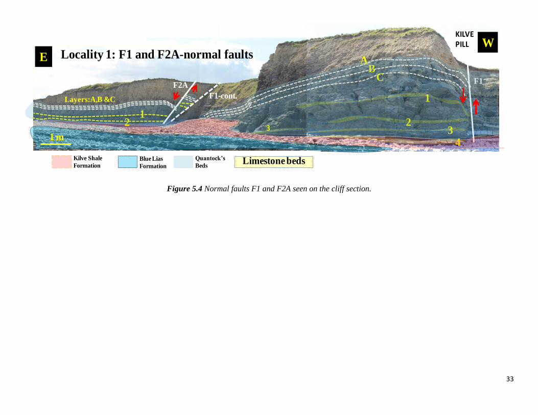
the process followed, while Figure 6.3 shows the detailed workflow used.
Figure 6.3 scheme showing the input data filtered in order to generated the horizons and fault surface
52
Figure 6.4 mapping workflow used
The Figure 6.6 (taken from Petrel), shows on the top, the fly photo of the locality 1 and 2, the dip
of the faults 2 and 5, and the layer 8 dip which goes across both faults. On the bottom left, it is
shown the use of the dummy point to generate surfaces, and on the bottom right, the faults 2 and
5 surface, as well as the layer 8 surface.

53
Dip measurements:1 layer and 2 faults (F2 and F5)
(Photo as basemap)
Dummy
points
Result= L8 surface in the faul block 2 and 2 fault surfacesMaking/edit
surface process
Legend
Strike
Dip
F5
F2
L8 surface generated
Locality 1 Locality 2
Figure 6.5 Petrel overview of the layer and fault surface procedure

54
The Isochors 3D modeling process was linked together to the layer surfaces previously done.
These isochors were checked according to the thickness measured on the field, and their
geological relationship following the stratigraphic framework defined above. A dominant
horizons and adding isochors with the high respective was done throw all segments in order to
visualize the 3D model and the behavior of the correlation between faults and horizons in the
Area. The Figure 6.4 shows the overview of the process used which generate 13 horizons by
block.
Figure 6.6 Make surface process
The Figure 6.8 shows on the top left the layer 8 surface and the contour map including the fly
photograph digitalized, On the top right, the layer 8 surface, the layer 11 isochrones generated the
fly photograph digitalized On the bottom left, the layers 8 and 11 surfaces, the fly photograph
digitalized and the contour map. And finally at the bottom right, the fly photograph digitalized,
indicating the locality 1 and 2, the layer 8 and 11 surface, and the contour map.

55
A) Take one layer surface by block B) Generate the isochors surfaces
C) View in 3D= L8 surface
and L11 isochors surfaces
D) Quality Check= consistency and match with the
base map (Photograph on this case)
L8 surface
L11 isochore surface
F2F5
L8 surface
Locality 1 Locality 2
Figure 6.7 Overview Isochors surfaces process by block

56
6.3 Structural Framework
This process enables faults and horizons to be modelled base on the inputs data given. (Petrel
Geology-2011). An overview in the volume calculations was included.
The horizon surfaces were chosen from top to down according to the stratigraphic sequences, in
addition, strike and dip measured were included. The faults were taken according to the general
striking (E-W) and dipping (most of them to the north) and three small reverse faults were
integrated to the model.
The fault model was built according to the input data using the grid points imported into Make
surfaces after these were imported in the “Fault Modeling” as straight fault pillars. The overview
of the process is shown in the Figure 6.5.
The faults surfaces were corrected in terms of faults length, orientation and matching with their
respective location into maps and photographs (Figure 6.6)
Figure 6.8 Fault Modelling Process
The Figure 6.10 shows on the top left the F2-F5 and F12 strike/dip measurements digitized on
the photographs with their respective surfaces created during the Make surface process, On the
top right, The 13 faults pillar generated and merged these with the photographs digitized showing
the F3 and F4 connection which was treated as one faults in the structural framework. On the
bottom , the two windows’ correspond to the quality check on the length and orientation of the
fault merged on the photographs digitized.

57
A) From strike/dip measurements= planar
surfaces were generated (F2, F5 and F12
respectively)C) 13 Fault Pillars ( with 2 faults connected=
F3 & F4 respectively)
B) Quality check= fault lengths, orientation and match with the photographs
Conection=
F3 & F4
F3
F4
F2 F5 F12
F2F5
F12F2
F5
F2
F5
F12
Figure 6.7 Fault modelling process: Faults (surfaces and pillars), connection and consistency between them

58
6.4 Fault diagnosis
In this study the fault diagnosis means to build and checked the quality of the faults as soon as
possible in order to speed the QC process. This process involved the fault data as input and its
modeling. The fault data point is converted in fault surface and then converted as fault stick or
fault polygon.
Into the pillar construction, the fault stick previously generated is the primary input doing a
conversion to key pillars that were displayed as X, Y and Z values (point location), it was
checked the faults individually passing for the fault block behavior and then verifying the
consistency on the all fault modeled in order to gridding these. In the group of fault models, it
was checked possible connection between them. Once finalized the QC of all faults a Pillar
gridding process as described in the Figure 6.12 was started resulting a skeleton in 3D with top-
mid and base surfaces.
Figure 6.10 Pillar gridding process
The Figure 6.12 shows on the top left the pillar gridding process where the faults interpreted
previously were merged in the fly photos checking the trend and connection of the fault on the fly
photographs, On the top right, verifying the 13 faults pillar consistency. On the bottom left, the
faults saving a good matching with the countour map and photographs digitized. On the bottom
right, the model skeleton showing the 3 surfaces that will define the model.

59
A) Pillar gridding process
B) QC in the fault modeling process in the contour map
D) Model Skeleton
D) Verify the fault pillars consistency
Top skeleton
Mid skeleton
Base skeleton
C) QC in the fault modeling process in the photograph
F14
F13F12
F11
F7F5F2
F1F3&F4
F8
Figure 6.11 Pillar gridding process: skeleton grid generation base on the key pillar defined in the previous process.

60
Locality 1 (Kilve Pill)
Locality 2Start Point F5
Locality 3Start Point F13
E Wa)
Beach Level
F1
F4
F7
F8
F9F10
F10-AF11
RED HOUSETop of the cliff
F7
4
1111
F5
b)
RELAY
RAMP
N
Loc 1Loc 2
Loc 3
Dome structures
F13
F1F2A
F3-RF
& F4
F14
F15
F8 F7F10-RF
F11
F9 F2-RF
Syncline 1
Syncline 2
12
4
77
Kilve Shale
FormationBlue Lias
Formation
Layer 7- limestone bed Layer 1 - limestone bed Layer 11- limestone bed
Quantock’s
Beds St. Audries
Shales
From Fieldwork
From Petrel
Figure 6.12 Fault interpretations: good comparison between fieldwork and Petrel. (Checking the god matching)

61
6.5 Model Segmentation
The stratigraphic horizons were inserted previously into the 3D model, and the layer surfaces
were projected near the faults according to establish in the make horizon process. The layers
projections realized by block, was used to show the fault displacement, keeping in mind that the
displacements data were not acquired in the fieldwork.
The horizons were selected according to the stratigraphy section (13 horizon surfaces generated
by block) and imported into Make horizons process, taking into account the fault modeling and
quality check in the input data. The output of the process mentioned above and showed in the
Figure 6.8 were eleven segments
Figure 6.13 Make horizon process
The Figure 6.15 shows on the top, 13 input horizons were identified and located according to
their fault block in the input selection. On the bottom, verifying if those input were sorted by the
stratigraphy sequences and gave the colour stratigraphy set defined before.
The Figure 6.16 shows two figures with an overview about the segmentation according to the
faults interpreted on the fly photographs digitized.

62
B) Quality check= Input horizons were sorted in the
correct stratigraphic order in the input pane
A) 13 horizons surfaces into 12 input horizon
defined according to the fault block
Surfaces Input horizons
Figure 6.14 Make horizons process includes interpreted horizons and QC in the stratigraphy show in 3D by intersection (Grid I-direction).

63
Segments legend
Locality 1
Locality 2
Locality 3
B0
B1
B2-3
B2
B5
B11
Figure 6.15 Make horizon process: Overview of Segmentation ( done by blocks).

64
6.6 Zone Properties and Layering Process
This process was realized in order to create the zones between the horizons and define the
vertical resolution in the model. The zones were added according to the thickness of the layer
collected on the field (Figure 6.3 and Figure 6.9 )
It was observed that the thickness of the beds increase towards to eastern (Early Lias formations)
Figure 6.17show in detail the Zones and layer distribution. The author made a review in the fault
modeling process to visualize the behavior of the layers. In addition, it was checked the pillar
gridding process to improve the model.
The quality check of the final 3D model was made by comparing the horizons the ones simulated
and the input data.
The final step of the structural framework was the layering process. It was implemented in order
to refine the grid by specifying the number of layers by zone division, following the top of the
zone (not included input data). The table 6.1 show a statistic for Kilve Beach 3D model.
The Figure 6.17shows on the left, an example the layer list to make zones with their respective
thickness value. On the right, verifying if those zone input was divided according to the
stratigraphy.

65
Table 6.2 Kilve grid Statistics
Axis Min Max Delta
X 483759.21 485024.96 1265.75
Y 5671179.64 5671645.38 465.74
Elevation depth [m] -59.43 121.58 181.00
Lat ~51°11'N ~51°11'N ~0°00'
Long ~3°13'W ~3°12'W ~0°01'
Description Value
Number of iconized horizons: 60
Number of iconized zones: 14
Number of faults: 12
Number of segments: 11
Number of properties: 13
Grid cells (nI x nJ x nGridLayers) 235 x 79 x 59
Grid nodes (nI x nJ x nGridLayers) 236 x 80 x 60
Total number of 3D grid cells: 1095335
Total number of 3D grid nodes: 1132800
Number of geological horizons: 60
Number of geological layers: 59
Geometry overview:
Vertical pillars: 0.00%
Linear pillars: 56.55%
Listric pillars: 43.45%

66
From top-L8 to top- L19
Make zones process
Figure 6.16Make zones process showing from top-L8 and top-L19 inserted geological zones in the stratigraphic intervals.

67
6.7 Property Modeling
This process was the distribution of the continuous (petrophysic) and discrete (facies) properties
in the 3D grid. The process was split in three sections
Geometrical Modeling
Facies Modeling
Petrophysical Modeling
Figure 6.17 Property Modeling scheme
6.7.1 Geometrical Modeling
Zones and segmentations were the properties generated on this section. These properties were
important for the volume calculation, also, in the facies and petrophysical properties operations.
6.7.2 Facies Modelling
A basic facies model was built conditioned to the outcrops observations (Limestone and shale)
represented by two models using the method sequential indicator simulation (SIS) in Petrel.
Model 1: Sand and shale only
Model 2: Using fine Sand, Coarse sand and shale facies
The variogram setting for both models was specified with the parameters show in the table below
for the sand facies while that for shale was assigned “0” value.

68
Table 6.1 Variogram setting for the sand facies.
Major dir. Range Minor Dir. Range Vertical Range Azimuth
Sand 50 50 10 16
Facies Models
A) Sand and Shale only
B) Sand: fine and Coarse
And shale
Figure 6.18 QC the facies models generated

69
6.7.3 Petrophysical Modeling
According to the facies properties, porosity, permeability and water saturations were assigned.
6.7.4 Contacts and Volumens
The GOC were defined at -10 m below to the base map surface and the volume in place was
calculated.
The Figure 6.20 shows on the left, the connected volume visualization distributed by colour
according to the number of layer assigned in the layering process. On the right, the facie property
using the model-2 for the visualization.
The Figure 6.21 shows the petrophysical and fluid properties generated and merged on the fly
photograps.
The Figure 6.22 shows the volume result spread sheet

70
A) Connected Volume
B) Facies: sand and shale
Figure 6.19 Geometrical modelling showing in 3D view: connected volume and facies property generated

71
A) Porosity property B) Permeability property C) Water Saturation property
Figure 6.20 Petrophysical and fluid properties

72
Petrel 2011.2 (64-bit) Schlumberger
User name l0281703
Date Fall semestre, 2012
Project kilve_VOLUMENS.pet
Model MODEL_KILVE BEACH
Grid Kilve_Grid
Input XY unit m
Input Z unit m
HC intervals Includes gas interval only.
Upper gas contact: Contact set\GWC
General properties
Porosity: PORO
Net gross: 1.00000000
Properties in gas interval
Sat. water: SW
Sat. gas: 1-Sw-So
Sat. oil: 0.00000000
Bg (formation vol. factor): 0.00020000 [rm3/sm3]
Rv (vaporized oil/gas ratio): 0.00000000 [sm3/sm3]
Recovery factor gas: 1.00000000
Properties in oil interval
Bo (formation vol. factor): 1.00000000 [rm3/sm3]
Rs (solution gas/oil ratio): 0.00000000 [sm3/sm3]
Recovery factor oil: 1.00000000
Case Bulk volume[*10^6 m3]Net volume[*10^6 m3]Pore volume[*10^6 rm3]HCPV oil[*10^6 rm3]HCPV gas[*10^6 rm3]STOIIP (in oil)[*10^6 sm3]STOIIP (in gas)[*10^6 sm3]STOIIP[*10^6 sm3]GIIP (in gas)[*10^6 sm3]GIIP (in oil)[*10^6 sm3]GIIP[*10^6 sm3]Recoverable oil[*10^6 sm3]Recoverable gas[*10^6 sm3]
Case 3 3 0 0 0 0 0 0 668 0 668 0 668
Segments
B1 0 0 0 0 0 0 0 0 9 0 9 0 9
B0 1 1 0 0 0 0 0 0 133 0 133 0 133
B8 0 0 0 0 0 0 0 0 24 0 24 0 24
B2 0 0 0 0 0 0 0 0 12 0 12 0 12
B2-3 1 1 0 0 0 0 0 0 83 0 83 0 83
B7 0 0 0 0 0 0 0 0 0 0 0 0 0
B5 0 0 0 0 0 0 0 0 21 0 21 0 21
B14 1 1 0 0 0 0 0 0 264 0 264 0 264
B13 0 0 0 0 0 0 0 0 65 0 65 0 65
B12 0 0 0 0 0 0 0 0 1 0 1 0 1
B11 0 0 0 0 0 0 0 0 56 0 56 0 56
Figure 6.21Volume results

73
7 Discussions
The technical framework from fault model was gotten from the data collected on the Kilve Beach
outcrops, Southwest of England. 18 faults were interpreted between cliff and beach exposures,
resulted of a correlation done by fault blocks added in the 3D geological model in Petrel. Below
in the Table 7.1, it is shown the number of faults interpreted in the area.
Table 7.1 Faults interpretation summary
Cliff Beach Both
Normal North 1 2 10
South 1
Reverse North 2
South 2
Fault interpretation numbersFaults Dip Direction
The stratigraphy framework was based on the limestone and shale beddings, they were dipping
towards the south following the stratigraphy sequences mapped by Brodahl, E. (1993), and
confirmed by the author according to the observations. (Figure 7.1 and Figure 6.14)
The fault analysis was done identifying the major faults (according to the measurements and fault
trough) and the faults associated to these combined with a view of the fault well exposed on the
outcrops in the zone. This combination resulted a better understanding of the structural
development of the area. (Figure 7.2, 5.9 and 6.12 respectively)
The strike and dip measurements in the faults and beds played an important role in the
consistency of the mapping result during the interpretation and understanding the fault behaviour.
The measurements and interpretation confirmed that the area is extensional. It confirms the
tectonic influence on deposition and stratigraphy framework was described by Tankard et. al
(1989).
In the mapping a minimum displacement was taken in the F1 (well exposed fault in the locality
1) giving 12 m as result, and recognized as planar fault in initiation stage due to the dip angle 45°
(fault initiation are typically in the range 45° and 60° according to Walsh et al., 1991).

74
Detailed interpretation on the bedding was done taking measurements on the strike, dip and
thickness in those places with good exposed and easily access. These values were performed
according to their stratigraphy and taken one horizon by block resulted of best matching with the
beach exposure photographs, the major number of the point or references acquired by GPS and
adding manually where was necessary in order to have more control points to build their surfaces
in Petrel.
In Petrel, the 10 most important fault blocks were defined, one was used as boundary on the east
of the area, and the fault defined was F15 which was dipping to the south. The beddings were
chosen by blocks as well and ideal model built in petrel suggested generate all surfaces as planar
due to the inconsistency that could be presented when the dip/strike measurements were loaded in
the surface. (Figure 7.15)
From the block-0 to block-5, the beding-8 was taken as main horizon where on the upper part
seven isochors were generated and in the lower part five isochors were generated. These horizons
and isochors were displayed and matched with the photographs. Only one measurement was
taken as fault displacement on the field. (Figure 7.5)
From the block-7 to block-15, the bedding-11 played as main horizon, generating 9 isochors on
the upper part and 3 isochors on the lower part. In terms to build an ideal model, the bedding
surfaces were assumed as flat plane (mentioned above) but in the reality were playing the dip and
strike over all bedding structures. Taking in account this condition in Petrel, the result was a good
matching between the beds and faults (Figure 7.5, 6.7 and 6.11 respectively). In addition the beds
thickness varies in the reality, the author took an average and saved it in order to generate in
Petrel for all the blocks and verify the consistency between them. In general terms, the horizons
had a good matching with the photographs taken as base map.
For the fault modelling, they were treated separately due to the different values in dip/strike and
direction exposed on the outcrops. The orientation consistency was checked with the faults pillar
into the pillar gridding process, also the visualizing if all of them were planar faults adding that
some of the small reverse faults interpreted on the reality were not taken into account in the 3D
model, only those one were easily to connect manually and finally gave an added value in the

75
structural development of the area. In the model, effectively the orientation of the faults towards
to the north was with striking variable according to the localities; and the orientation of the beds
towards to the south; the striking was matched E-W as the interpretations on the field.
Into the 3D model the facies distribution were divided by two models, one with only sand and
shale ( Model 1- assigned values) and where the facies were mixed as sand fine, sand coarse and
shale going through the horizons defined according to the stratigraphy framework generated
previously (Figure 7.18). In addition, a connected volume facies was generated in order to see
which package of sand or sand bodies were connected between the fault blocks.
The petrophysical properties were taken assigning parameters, varying the porosity beet 0-shales
and 25% -sand and permeability between 0 mD shale, 100mD for sand fine and 1000 mD for
sand facies.
In the area of the study, it was located a relay ramps, which can be important location for
hydrocarbon migration because they link the hanging walls and footwalls of fault systems
(Larsen, 1988; Peacock and Sanderson 1994). Flow can occur from the hanging wall, which may
be a basin, up the ramp to the footwall. They can be also important location of hydrocarbon traps
because of the folding and networks of small-scale faults that occur in ramps (Gawthorpe, R. L.,
and J. M. Hurst, 1993, Peacock and Sanderson 1994)
This project is a good example where by integrating the data collected in the field, pass through
the fault and horizon processes with the objective the create a 3D model that allow to understand
the structural behaviour of the locality, and predict or search an approach which could generate
the hydrocarbons traps.

76
8 Conclusions
The Kilve outcrops have been characterized as natural laboratory due to their complexity of the
normal fault systems. In the area of the study, it was located a relay ramps which could be used as
guideline for hydrocarbons traps prediction. The relay ramps can reorient strata that connect the
hanging wall and footwall of normal fault system. The strike and dip measurements in the faults
and beds played an important role in the consistency of the mapping result during the
interpretation and understanding the fault behaviour. The measurements and interpretation
confirmed that the area is extensional
The Kilve Beach area is dominated lithologically by mudstones and interbedded with limestones
beds. From Observations in the locality 3 we can say that the Early Jurassic Blue Lias Formation
is dominated structurally by WNW trending. Tthickness of the beds increase towards to eastern
(Early Lias formations)
The stratigraphy framework was based on the limestone and shale beddings, they were dipping
towards the south following the stratigraphy sequences mapped by Brodahl, E. (1993), and
confirmed by the author according to the observations.
18 faults were interpreted on the outcrops and 11 faults (8 were interpreted as normal and 3 as
reverse) were included in 3D geological model using Petrel ™ software (small reverse faults and
those exposed only in the cliff section were exclude), in addition, 13 horizons were generated
taking in account the stratigraphic sequences. The fault and horizons gave a good matching on
the photographs digitized and with the interpretations done in the field.
Facies and petrophysical properties were added given as result volume calculation simulating a
gas field (GIIP (in gas) = 668[*10^6 sm3])

77
9 Recommendations for further work
Increase the density of data collected by km2
in order to improve the resolution of the model.
Extend the study area to the surrounding of Kilve Beach, and integrate the seismic, logs and
petrophysics interpretations available from the area.
Include a facies approach in the fault zone with high content of fractures, where the vertical
component plays an important role providing certain constrain in 3D geological model.
Build a reservoir simulation model by using data from the North Sea fields. The simulation
model should include sensitivities in order to correlate the faults modeled and the transmissibility
computed by the reservoir simulator. This is especially important because of the large number of
fields in the North Sea which its developments are linked to the fault behavior.

78
10 References
Antonellini M., Aydin A., 1994, Effect of faulting on fluid flow in porous sandstones:
petrophysical properties: The American Association of Petroleum Geologists Bulletin, v. 78,
p 335–377
Bartley, J. M., and A. F. Glazner, 1991, En echelon Miocene rifting in the southwestern United
States and model for vertical-axis rotation in continental extension: Geology, v. 19, p. 1165–
1168
Beach, A., 1989 the geometry of normal faults—examples from the Jurassic of Somerset (abs.):
Geological Society of London Meeting, The Geometry of Normal Faults, London, June 14–
15.
Bowyer, M.O.N., and Kelly, P.G. 1995. Strain and scaling relationships of faults and veins in
Kilve, Somerset . Proceeding of the Ussher Society, v.8, p 411-416.
Brodahl, E. (1993). Fault Pattern in nord Somerset . Unpublished thesis for candidature of
Geology and rocks mechanics . University of Trondheim, 72 p .
Caine, J. S., James, P. E. & Forster, G. B., 1996. Fault zone architecture and permeability
structure. Geology 24 (11), p 1025-1028.
Cornford, C.,1986, The Bristol Channel Graben: organic geochemical limits on subsidence and
speculation on the origin of inversion. Proceeding of the Ussher Society, v.6, p 360-367.
Cornford, C.,2003, Triassic palaeo-pressure and Liassic mud volcanoes near Kilve, West
Somerset. Geoscience in south-west England, v.10, p 430-434.

79
Cox, B.M., Sumbler, M.G. & Ivimey-Cook, 1999. A formational framework for the Lower
Jurassic of England and Wales (on shore area). BGS research report RR/99/01
Edwards, R.A., 1999, The Minehead district—a concise account of the geology, Memoir for
1:50,000 Geological Sheet 278 and part of sheet 294 (England and Wales). British
Geological Survey, the Stationery. Office, London.
Engelder, T. and Peacock D. C. P. 2001. Join development normal to regional compression
during flexure-flow folding: the Lilstock buttress anticline, Somerset, England. Journal of
Structural Geology 23, p 259-277
Fredman, Niclas; Tveranger, Jan; Cardozo, Nestor; Braathen, Alvar; Soleng, H. H.; Røe, P.;
Skorstad, A.; Syversveen, A. R.; 2008. Fault facies modelling; technique and approach for
3D conditioning and modelling of faulted grids AAPG Bulletin 92, no. 11, p. 1457-1478.
Gawthorpe, R. L., and J. M. Hurst, 1993, Transfer zones in extensional basins: their structural
style and influence on drainage development and stratigraphy: Journal of the Geological
Society of London, v. 150, p. 1137–1152.
Glen, R.A., hancock, P.L. and Wittaker, A., 2005, Basin inversion by distributed deformation: the
southern margin of the Bristol Channel Bassin, England: Journal of Structural Geology,
v.27, p 2113-2134.
Jones, G., Fisher, Q.J., and Knipe, R.J., eds., 1998,Faulting, Fault Sealing and Fluid Flow
inHydrocarbon Reservoirs: Geological Society of London Special Publication 147, 319 p.
Kamerling, P. 1979. The geology and hydrocarbon habitat of the Bristol Channel Basin. Journal
of Petroleum Geology 2 (1), p 75-93.

80
Kelly, P.G., 1998. Development and Interaction of Segmented Fault Systems. Unpublished Ph.D.
thesis, University of Southampton, 167 p.
Kim, Y.S., Peacock D. C. P., Sanderson D. J. 2004. Fault damage zones. Journal of Structural
Geology, v.26, p 503-517.
Knipe R. J., Fisher Q. J., Jones G., 1997.In Hydrocarbon Seals: Importance for Exploration and
Production, Fault seal analysis: successful methodologies, application and future directions,
NPF Special Publication, eds Moller-Pedersen P., Koestler A. G. 7, p 15–40
Knott S. D. 1993 Fault seal analysis in the North Sea. American Association of Petroleum
Geologists Bulletin 77, p 778–792
Larsen, P.-H., 1988. Relay structures in a Lower Permian basement- involved extension system,
East Greenland: Journal of Structural Geology, v. 10, p. 3–8.
Lindanger, M., 2003. A study of rock lenses in extensional faults, focusing on factors controlling
shapes and dimensions. Unpublished thesis for Candidatus Scientiarum degree. University of
Bergen, 166 pp.
Mandl, G., 1988. Mechanics of tectonic faulting: Models and basics concepts, Amsterdam,
Elseiver, 407 p
Masson, D.G., and P.R. Miles, 1986a, Development and hydrocarbon potential of Mesozoic
sedimentary basins around margins of North Atlantic: American Association of Petroleum
Geologists Bulletin, v. 70, p. 721-729.
Millson, J., 1987, The Jurassic evolution of the Celtic Sea basins, in J. Brooks and K.W. Glennie,
eds., Petroleum geology of North West Europe: London, Graham and Trotman, p. 599-610

81
Palmer, C.P. 1972. The Lower Lias (Lower Jurassic) between Watchet and Lilstock in North
Somerset (United Kingdom). Newsletter of Stratigraphy, v.2, p 1-30.
Peacock D. C. P., Sanderson D. J. 1994. Geometry and development of relay ramps in normal
fault systems. American Association of Petroleum Geologists Bulletin 78, p 147–165.
Peacock D. C. P., Sanderson D. J. 1995. Strike-slip ramps. Journal of Structural Geology, v.7, p
1351-1360
Peacock D. C. P., Sanderson D. J. 1999. Deformation history and basin-controlling faults in the
Mesozoic sedimentary rocks of Somerset coast. Proceeding of the Geological Association,
110, p 41-52.
Roberts, A.M, Yielding, G., and Freeman, B., 1991. The geometry of normal faults. Journal of
the Geological Society, London, Special Publications v.147, p. 185-187.
Simms, M.J., Chidlaw, N., Morton, N. & Page, K.N., 2004, British Lower Jurassic Stratigraphy,
Geological Conservation Review Series, No. 30, Joint Nature Conservation Committee,
Peterborough, 458 p
Steen Øyvind, 1995. Field observations to test methods for identification of faults using dipmeter
logs; examples from Kilve in South England. Reservoir Techn. Report. 17 p
Tankard, A.J. and Balkwill, H.R. 1989. Mesozoic History of the Celtic Sea Basins: Chapter 28:
Extensional Tectonics and Stratigraphy of the North Atlantic Margins. Tulsa, American
Association of Petroleum Geologists . p 433-444

82
Tappin, D.R., Ciiadwick, R.A., Jacson, A.A., Wingfielo, R. T.R and Smith, N.J.P., 1994.The
Geology of Cardigan Bay and The Bristol Channel. United Kingdom Offshore Regional
Report. British Geology Survey.
Townsend, C., Firth, I., Westerman, R., Kirkevollen, L., Harde, M., Andersen, T., 1998. Small
seismic-scale fault identification and mapping, In: Jones, G., Fisher, Q.J., Knipe, R.J. (Eds.),
Faulting, fault sealing and fluid flow in hydrocarbon reservoirs. Geological Society, London,
Special Publications, pp. 1-25.
Van der Zee W., Urai J.L., 2005. Processes of normal fault evolution in a siliciclastic sequence: a
case study from Miri, Sarawak, Malaysia. Journal of Structural Geology 27, p. 2281–2300
Van Hoorn, B., 1987, The South Celtic Sea/Bristol Channel basin: origin, deformation and
inversion history, in P.A. Ziegler, ed., Compressional intraplate deformations in the Alpine
foreland: Tectonophysics, v. 137, p. 309-334.
Walsh J. J., Watterson J. 1992. Populations of faults and fault displacements and their effects on
estimates of fault-related regional extension. Journal of Structural Geology 14, p 701–712
Walsh J. J., Watterson J. (1991) in The Geometry of Normal Faults, Geometric and Kinematic
coherence and scale effects in normal fault systems, Geological Society, London, Special
Publications, eds Roberts A. M., Yielding G., Freeman B. 56, p 193–203
10.1 Maps References
Quantock Hills and Bridgwater maps -1:25000 scale digitized in ANQUET MAPS 2011 (a
program commercially available on the Ordnance Survey in UK)
10.2 Manual references
Petrel Geology course. 2011. Schlumberger.

83
11 Appendix
11.1 Raw data collected-GPS points
Table 11.1 GPS points collected in the area according to the fault block
NAME X Y Fault Block
F1 484267,481 5671435 1
F1D 484261,55 5671437,91 1
F2C1 484330,007 5671406 2
F2D 484310,157 5671450,66 2
F2D1 484323,92 5671449,51 2
F2D2 484340,89 5671445,67 2
F2L9 484228,624 5671456,69 2
F3D1- 484348,435 5671444,87 3
F3D2- 484370,515 5671444,25 3
F3D3- 484383,99 5671440,09 3
F3L6A 484333,069 5671447,48 3
F3L6AB 484326,991 5671448,27 3
F3L7A 484322,456 5671450,4 3
F3L7AB 484318,053 5671450,53 3
F3L8A 484310,511 5671451,99 3
F3L8AB 484302,826 5671452,91 3
F3L9U 484258,199 5671461,83 3
F3U 484450,828 5671450,46 3
F4D1 484508,938 5671463,07 4
F4D2 484494,483 5671466,56 4
F4D3L9 484473,312 5671467,63 4
F4D4L10 484450,753 5671471,81 4
F4D5L10&3 484419,035 5671474,46 4
F4D6L10 484389,347 5671478,11 4
F4DL1 484514,322 5671464,05 4
F4L2 484501,69 5671469,43 4
F4U 484543,756 5671468,86 4
F5end 484515,114 5671471,95 5
F5L1 484527,137 5671473,02 5
F5U 484582,746 5671490,76 5
F6U 484598,561 5671498,17 6
F6U2 484613,27 5671509,35 6
F7AL2 484554,451 5671516,2 7
F7BL1 484567,29 5671486,58 7
F7D 484595,488 5671545,33 7
F7D1 484588,926 5671547,35 7
F15-1 484706,862 5671610,61 14
F15-2 484725,954 5671615,67 14
F15-3 484737,697 5671616,64 14
NAME X Y Fault Block
AftRH 484902,1 5671578 13
AftRH2 484915,3 5671592 13
AftRH3 485006,5 5671641 13
AftRH4 485052,5 5671706 15
AftRH5 485079,8 5671741 15
DC1L8 484224,3 5671434 1
DC2L6 484245,7 5671435 1
DC3L3 484270,6 5671433 1
DC4L4 484292,6 5671435 1
DC5L4 484304 5671437 5
DC6L3 484330,4 5671430 7
L10D1 484253,2 5671454 1
L10D10 484540,8 5671484 1
L10D11 484541,4 5671489 1
L10D2 484281,7 5671462 1
L10D3 484322,7 5671469 1
L10D4 484349 5671468 1
L10D5 484405,4 5671468 1
L10D6 484460,2 5671461 1
L10D7 484479,7 5671462 1
L10D8 484505,6 5671459 1
L10D9 484525,1 5671456 1
L10F6-1 484540,4 5671481 1
L10Rev 484567,7 5671494 1
L11-1 484228,2 5671457 1
L11F1AR 484193,6 5671446 1
L11F2ARR 484198,2 5671447 1
L11F3AB 484255,9 5671457 2
L11F3AR 484259 5671458 2
L11F6 484529 5671488 5
L11F6B 484539,2 5671484 5

84
11.2 Fault data collected on the cliff section.
Table 11.2 Dip and strike values taken in the cliff section
Fault name Dip Angle Direction
F1
CLIFF3
F2 61N N12W
F3 52N N55W
F4-A 43N N15W
F4 43N N75W
F5 61N N10W
F7 48N N20W
F8-A 20N N10E
F8 68N N10W
F9 89NE N2W
F10 76N N5W
F12 65N N3W
F13 89N N5W
F14 47S N3W
43N N15W