In preparation for Journal of Climate

GFDL’s CM2 global coupled climate models-Part 2: The baseline ocean

simulation

Anand Gnanadesikan♦∗, Keith W. Dixon♦, Stephen M. Griffies♦, V. Balaji♣, Marcelo

Barreiro♣, J. Anthony Beesley♣, William F. Cooke♥, Thomas L. Delworth♦, Rudiger

Gerdes ♠, Matthew J. Harrison♦, Isaac M. Held♦, William J. Hurlin♦, Hyun-Chul Lee♥,

Zhi Liang♥, Giang Nong♥, Ronald C. Pacanowski♦, Anthony Rosati♦, Joellen Russell♣,

Bonita L. Samuels♦, Qian Song♣, Michael J. Spelman♦, Ronald J. Stouffer♦, Colm O.

Sweeney♣ Gabriel Vecchi♣, Michael Winton♦, Andrew T. Wittenberg♦, Fanrong Zeng♥,

Rong Zhang♣

♦NOAA Geophysical Fluid Dynamics Laboratory

PO Box 308, Forrestal Campus, Princeton, New Jersey, 08542 USA

♣Program in Atmospheric and Oceanic Sciences

Princeton University, Princeton, New Jersey, 08542 USA

♥RS Information Systems

McLean, Virginia, presently at GFDL

♠ Alfred Wegener Insitute for Polar and Marine Research

Bremerhaven, Germany

(Draft 8 December 2004)

ABSTRACT

The current generation of coupled climate models run at the Geophysical Fluid Dynamics Laboratory as partof the Climate Change Science Program contain ocean components that differ in almost every respect from thosecontained in previous generations of GFDL climate models. This paper summarizes the new physical features ofthe models and examines the simulations that they produce. Of the two new coupled models, the CM2.1 modelrepresents a major improvement over CM2.0 in most of the major oceanic features examined, with strikingly lowerdrifts in hydrographic fields such as temperature and salinity, more realistic ventilation of the deep ocean, andcurrents that are closer to their observed values. Regional analysis of the differences between the models highlightsthe importance of wind stress in determining the circulation, particularly in the Southern Ocean. At present,major errors are associated with Northern Hemisphere Mode Waters and outflows from overflows, particularly theMediterranean Sea.

1 Introduction

A major part of developing a ”realistic” model ofthe climate system is the development of a model

∗Corresponding author: Anand.Gnanadesikan@noaa.gov

of ocean circulation. The ocean circulation playsan important role in earth’s climate. By transport-ing heat to polar latitudes, it plays a major role inmaintaining the habitability of such regions (Man-

1

2 GFDL Ocean Model Development Team

abe and Bryan,1969). Indeed, recent work by Win-ton (2003) suggested that in the absence of oceanheat transport, the planet would glaciate. Manabeet al. (1991) and Stouffer (2004) show that theocean determines the spatial pattern and temporalscale of response to changes in the surface radia-tion balance. However, despite many decades of re-search different ocean general circulation models stillyield solutions that differ in important ways. Recentwork as part of the Ocean Carbon Model Intercom-parison Project (OCMIP), which involved compar-isons between ocean-only models run by 13 groups,showed large differences in overturning streamfunc-tion (Doney et al. 2004) and the rate of ventilation inthe Southern Ocean (Matsumoto et al., 2004). Suchdifferences have important implications for climatechange. Models with weak Northern Hemisphereoverturning circulations would be expected to havetoo large a response to changes in hydrological cy-cling (Stommel, 1961, though as the companion pa-per by Stouffer et al. shows this is not always thecase). Models which maintain high levels of convec-tion in the Southern Ocean may also have too stronga response to an increase in the hydrological cycle,cutting off convection that does not exist in the realworld. Such differences could have major implica-tions for ocean ecosystems, which are very dependenton the rate of vertical exchange (Gnanadesikan et al.,2002) and for the response of the carbon cycle to cli-mate change (Sarmiento et al., 1998).

Understanding such issues is particularly challeng-ing in ocean models because of questions aboutthe impact of numerics. Processes known to havean important impact on vertical exchange in level-coordinate models include numerical diffusion result-ing from truncation errors associated with advection(Griffies et al., 2001), truncation errors associatedwith isopycnal mixing (Griffies et al., 1998), convec-tive entrainment in overflows (Winton et al., 1998),and high levels of background lateral diffusion. Thepast decade has seen sustained effort in the mod-eling community at large to address some of themore egregious numerical shortcomings in models.At GFDL, we have developed a new ocean code, theModular Ocean Model Version 4.0 (MOM4, Griffieset al., 2003) in which almost every aspect of the ocean

model from the free surface to the bottom boundarywas revisited.

This new code has been used to configure two mod-els which are run as part of the coupled models CM2.0and CM2.1 (Delworth et al., this issue). The twomodels are very similar, differing only in a few sub-gridscale parameterizations and in the timesteppingscheme. While the ocean-only versions of these mod-els are referred to at GFDL by the nomenclatureOM3.0 (for the model used in CM2.0) and OM3.1 (forthe model used in CM2.1) in this paper we will sim-ply identify the ocean models by the coupled model ofwhich they are a part (since we will only be presentingsolutions from these coupled models). This paper ex-amines the ocean circulation produced by the CM2.0and CM2.1 coupled models. In particular, it looks atthe following questions:

1. How well does the model simulate the large-scalehydrography and flow fields?

2. What are the principal errors in hydrographyand flow fields made by the models?

3. How do these differ between CM2.0 and CM2.1?

Our goal is both to document lessons learned fromrunning the pair of models and to highlight areaswhere the model circulation is greatly in error. Inthe latter case, we note that it would be unwise forother investigators to draw strong conclusions aboutthe effects of climate change based on features thatare not well simulated. Section 2 gives a brief de-scription of the numerical formulation of the oceanmodel. Section 3 looks at global diagnostics of thesimulation. Section 4 examines some diagnostics ofthe circulation in five regions; the Southern Ocean,the North Atlantic, the North Pacific, the NorthernIndian and the Arctic. The tropical Pacific (which iswell represented in both models) is discussed in detailin the companion paper of Wittenberg et al. (2005)and the tropical Atlantic will be discussed in a paperby Barreiro et al. (in prep.). Section 5 concludes thispaper.

3

2 Model formulation

a. Common features of the models

The GFDL ocean model presented here differs sig-nificantly from that used in previous assessments. Asummary of the differences is provided below. Fora more detailed discussion of the model formulationthe reader is referred to Griffies et al. (in prep.).

The ocean model is of significantly higher resolu-tion than the 4 degree, 12-level model (Manabe andStouffer, 1991) used in the IPCC First AssessmentReport and the 2 degree, 18-level model (Delworth etal.,2003) used in the Third Assessment Report. Thelongititudinal resolution of the CM2 series is 1 degreeand the latitudinal resolution varies between 1 de-gree in the mid latitudes and 1/3 degree in the trop-ics, where higher resolution was needed to resolve theequatorial wave guide. A tripolar grid (Murray, 1996)is used to move the polar singularity onto the land,allowing for resolved cross-polar flow and eliminatingthe necessity to filter fields near the pole. There are50 vertical levels with 22 uniformly spaced over thetop 220m. Below this depth, the thickness increasesgradually to a value of 366.6m at the ocean bottom,which is located at a depth of 5500m.

In contrast to previous models which used therigid-lid approximation to solve for the surface pres-sure, the CM2 models use an explicit free surface(Griffies et al., 2001). This allows for real fluxesof freshwater, in contrast to the ”virtual salt fluxes”used by most ocean models. However, the use of realfreshwater fluxes introduces a number of new prob-lems. The first is that the free surface thins whenwater freezes into sea ice. This can result in numeri-cal instability when sea ice approaches the thicknessof the top box. In the CM2 models this is solved bylimiting the ice weight on the ocean to 4m of ice evenwhen the ice thickness exceeds 4m. Second, riversbe handled in a special way, inserting fluid into theocean instead of fluxing salt. Third, narrow pas-sages that connect marginal seas to the main bodyof the ocean, which in past models were representedby stirring fluid between boxes separated by land,must allow for a net flow of mass to prevent exces-sive buildup or drawdown of water in these marginal

basins. Finally, using a real freshwater flux can resultin nonconservation of certain tracers when traditionalleapfrog timestepping schemes are used. More discus-sion of these issues is provided in Griffies et al. (inprep.).

The models also incorporate a number of improve-ments in upper ocean physics. The mixed layer is pre-dicted using the KPP mixed layer scheme of Large etal. (1994). Shortwave radiation absorption is repre-sented using the optical model of Morel and Antoine(1994) with a yearly climatological concentration ofchlorophyll from the SeaWIFS satellite. The princi-pal impact of including variable penetration of short-wave radiation is found in the tropics in ocean-onlymodels (Sweeney et al., in press).

The representation of near-bottom processes hasalso been improved in the CM2 model series. Bot-tom topography is represented using the method ofpartial cells (Adcroft et al., 1997; Pacanowski andGnanadesikan, 1998), and is thus much less sensitiveto the details of vertical resolution. Better repre-sentation of the details of bottom topography doesnot, however, solve one of the most persistent prob-lems of level-coordinate models, namely the tendencyto dilute sinking plumes of dense water (Winton etal., 1998). In order to ameliorate the effects of this”convective entrainment” a primitive representationof bottom boundary layer processes (following Beck-mann and Doscher, 1998) has been added in whichfluid is mixed along the slope when dense water isfound upslope of light water. This parameterizationhas relatively little effect on the magnitude of theoverturning and heat transport, but its effects can beseen in tracer fields such as salinity and age.

The interaction of tides with the ocean bottom canserve as a major driver of mixing. In shallow regions,large tidal velocities can directly generate high levelsof turbulence. In the CM2 model series this effectwas parameterized by adding a source of turbulentkinetic energy based on a global model of tides tothe bottom-most level in the KPP scheme. More de-tails are presented in Lee et al., (subm.). As dicussedin this paper, tidal mixing resulted in a substantialreduction in Arctic stratification and helps reduce ex-cessively low salinities at certain river mouths. How-ever, it did not have a major impact on the overturn-

4 GFDL Ocean Model Development Team

ing circulation or on temperature drifts.The interaction of tides with the ocean bottom can

also produce internal waves which propogate upwardsin the water column and break. Because the deepocean is less stratified than the pycnocline, this pro-duces relatively high levels of vertical dissipation inthe deep ocean (Polzin et al., 1997). For many years,GFDL models have attempted to represent this effectby having the vertical diffusion transition between arelatively low value (0.15-0.3 cm2/s) in the pycnoclineand a relatively high value (1.0-1.3 cm2/s) in the deepocean (Bryan and Lewis, 1979). The present modeluses the same pycnocline value of 0.3 cm2/s as pre-vious models polewards of 40◦ in both hemispheres,with a lower value of 0.15 cm2/s in the low latitudes.The lower tropical value is clearly justified by theresults of the North Atlantic Tracer Release Exper-iment (Ledwell et al., 1993), by turbulence profilingalong the equator (Peters et al., 1989), and by sim-ulations showing that such a high value of turbulentdiffusion can lead to excessive deep upwelling at theequator (Gnanadesikan et al., 2002). An even highervalue of vertical diffusion than the one we have usedmay be justified within the Southern Ocean where in-ternal wave activity is known to be enhanced (Polzin,1997), but the value used in the Arctic is likely stilltoo high, given that internal wave activity is knownto be very low there (Levine et al., 1984). A valueof 1.2 cm2/s is used in the deep ocean. While somerecent schemes (Simmons et al., 2004) allow for deepmixing to be spatially variable, they were not judgedmature enough for inclusion into this version of thecoupled model when the model was frozen.

In addition to lowering the vertical mixing in thesubtropical thermocline, a number of other changeswere made to the physics in the model interior. Oneis that the advection scheme was changed from thecentered-difference scheme used in previous versionsof the model to the flux-corrected scheme utilized inthe MIT general circulation model. This scheme isbased on the third-order upwind-biased approach ofHunsdorfer and Trompert (1994) which employs theflux limiters of Sweby (1984) to ensure that tracers donot go out of bounds. Additionally, the lateral mixingof both tracers and momentum is considerably moresophisticated than in previous versions of the model.

Because there are important differences in how thelateral mixing is implemented between CM2.0 andCM2.1, we discuss these separately in two sectionsbelow.

b. Isoneutral mixing parameterization

There are two key characteristics of the mixing as-sociated with eddies. First, eddies within the oceaninterior tend to homogenize tracers along surfaces ofconstant neutral density (Ledwell et al., 2001). In nu-merical models of ocean circulation one of the tracersthat tends to be homogenized in this way is potentialvorticity (Rhines and Young, 1982). On a flat f-plane,the PV homogenization corresponds to an advectiveflow that homogenizes interface heights. Such flowsare parameterized in CM2 according to the parame-terization of Gent and McWilliams (1990) as imple-mented by Griffies (1998). Essentially, one can thinkof eddies as leading to an advective flow given by

M = (∂/∂z)(κS) (1)

where κ is a diffusive coefficient and S is the isopycnalslope. Completing the closure requires a closure fordealing with κ, particularly as S goes to infinity inthe mixed layer.

In CM2.0 and CM2.1 κ is a function of the horizon-tal density gradient averaged over the depth range of100 to 2000m. The formula for κ is

κ = α |∇zρ|z

(

L2 g

ρo No

)

. (2)

Here, α is a dimensionless tuning constant set to0.07, L is a constant length scale set to 50km, No

is a constant buoyancy frequency set to 0.004 s−1,g = 9.8 ms−1 is the acceleration of gravity, ρo =1035 kgm−3 is the reference density for the Boussi-nesq approximation, and |∇zρ|

zis the average of

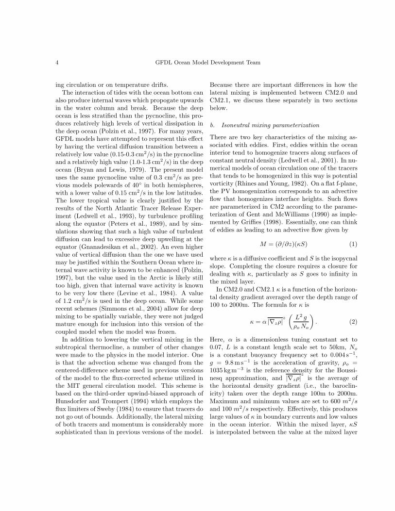
the horizontal density gradient (i.e., the baroclin-icity) taken over the depth range 100m to 2000m.Maximum and minimum values are set to 600 m2/sand 100 m2/s respectively. Effectively, this produceslarge values of κ in boundary currents and low valuesin the ocean interior. Within the mixed layer, κSis interpolated between the value at the mixed layer

5

base and a value of 0 at the surface. Figure 1 showsa map of κ in CM2.0.

In CM2.0 the isopycnal mixing coeffficient AI isidentical to κ. In CM2.1 it is maintained at a valueof 600 m2s−1 throughout the ocean. This differencewas found to reduce sea ice biases, particularly inthe North Pacific. While it has a relatively smalleffect (documented in more detail in Griffies et al.,in prep.) this choice represents an attempt to tuneaway a model bias, rather than an attempt to makea poorly represented process more physical.

Figure 1: Isoneutral diffusion coefficient κ in m2s−1 inCM2.0.

c. Lateral viscosity parameterization

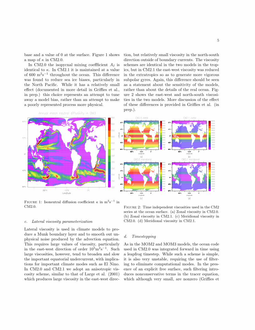
Lateral viscosity is used in climate models to pro-duce a Munk boundary layer and to smooth out un-physical noise produced by the advection equation.This requires large values of viscosity, particularlyin the east-west direction of order 105m2s−1. Suchlarge viscosities, however, tend to broaden and slowthe important equatorial undercurrent, with implica-tions for important climate modes such as El Nino.In CM2.0 and CM2.1 we adopt an anisotropic vis-cosity scheme, similar to that of Large et al. (2001)which produces large viscosity in the east-west direc-

tion, but relatively small viscosity in the north-southdirection outside of boundary currents. The viscosityschemes are identical in the two models in the trop-ics, but in CM2.1 the east-west viscosity was reducedin the extratropics so as to generate more vigoroussubpolar gyres. Again, this difference should be seenas a statement about the sensitivity of the models,rather than about the details of the real ocean. Fig-ure 2 shows the east-west and north-south viscosi-ties in the two models. More discussion of the effectof these differences is provided in Griffies et al. (inprep.).

Figure 2: Time independent viscosities used in the CM2series at the ocean surface. (a) Zonal viscosity in CM2.0.(b) Zonal viscosity in CM2.1. (c) Meridional viscosity inCM2.0. (d) Meridional viscosity in CM2.1.

d. Timestepping

As in the MOM2 and MOM3 models, the ocean codeused in CM2.0 was integrated forward in time usinga leapfrog timestep. While such a scheme is simple,it is also very unstable, requiring the use of filter-ing to eliminate computational modes. In the pres-ence of an explicit free surface, such filtering intro-duces nonconservative terms in the tracer equation,which although very small, are nonzero (Griffies et

6 GFDL Ocean Model Development Team

al., 2001). Moreover, using a leapfrog timestep re-quires keeping track of two sets of solutions (on oddand even timesteps). However, the maximum al-lowable timestep is that which results in instabilitywhen integrating the equations on the odd (or even)timesteps using forward integration. By switchingto a more sophisticated forward integration one caneliminate one set of solutions, greatly increasing thespeed of the model. This was done in CM2.1. Chang-ing the timestepping scheme has a small impact onthe solution in most parts of the model, though somechanges are seen right on the equator. More dicussionof this issue is provided in Griffies et al. (in prep.).

e. Simulation protocol

The simulations are initialized from the World OceanAtlas (2001) data for temperature and salinity. Twosets of control runs are done, one using 1990s radia-tive conditions with a net ocean heating of around 1Wm−2 and one using 1860s radiative conditions witha net ocean heating of 0.3 Wm−2 (see Figure 3 ofDelworth et al., this issue ). In previous versions ofthe GFDL coupled model the atmosphere was spunup for many years using prescribed sea surface tem-peratures, the ocean was spun up over many yearsusing the output of the atmospheric model, and fluxadjustments were computed by restoring the surfacetemperatures and salinities to observations within theocean-only model. The combined model was thencoupled. In the present series of models this is notdone. Instead, the models are essentially initializedfrom initial conditions and allowed to drift withoutflux adjustments.

One of the drawbacks of this approach is that itis not clear how to compare the model with observa-tions. Modern observations have been taken during aperiod when the climate has a trend. The model mayor may not be in a similar balance. Since the datais largely modern, we decided to present simulationsfrom our 1990 control runs, which as documented inDelworth et al. (this issue) have relatively little driftin sea surface temperatures. Data is presented fromthe years 101-200 of these control runs, with the ex-ception of ideal age, where years 65-70 are used tofacilitate comparison with observations.

3 Global-scale diagnostics

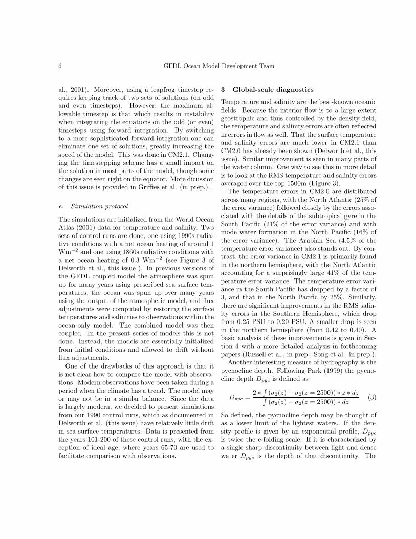
Temperature and salinity are the best-known oceanicfields. Because the interior flow is to a large extentgeostrophic and thus controlled by the density field,the temperature and salinity errors are often reflectedin errors in flow as well. That the surface temperatureand salinity errors are much lower in CM2.1 thanCM2.0 has already been shown (Delworth et al., thisissue). Similar improvement is seen in many parts ofthe water column. One way to see this in more detailis to look at the RMS temperature and salinity errorsaveraged over the top 1500m (Figure 3).

The temperature errors in CM2.0 are distributedacross many regions, with the North Atlantic (25% ofthe error variance) followed closely by the errors asso-ciated with the details of the subtropical gyre in theSouth Pacific (21% of the error variance) and withmode water formation in the North Pacific (16% ofthe error variance). The Arabian Sea (4.5% of thetemperature error variance) also stands out. By con-trast, the error variance in CM2.1 is primarily foundin the northern hemisphere, with the North Atlanticaccounting for a surprisingly large 41% of the tem-perature error variance. The temperature error vari-ance in the South Pacific has dropped by a factor of3, and that in the North Pacific by 25%. Similarly,there are significant improvements in the RMS salin-ity errors in the Southern Hemisphere, which dropfrom 0.25 PSU to 0.20 PSU. A smaller drop is seenin the northern hemisphere (from 0.42 to 0.40). Abasic analysis of these improvements is given in Sec-tion 4 with a more detailed analysis in forthcomingpapers (Russell et al., in prep.; Song et al., in prep.).

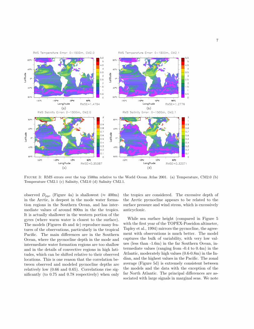
Another interesting measure of hydrography is thepycnocline depth. Following Park (1999) the pycno-cline depth Dpyc is defined as

Dpyc =2 ∗

∫

(σ2(z) − σ2(z = 2500)) ∗ z ∗ dz∫

(σ2(z) − σ2(z = 2500)) ∗ dz(3)

So defined, the pycnocline depth may be thought ofas a lower limit of the lightest waters. If the den-sity profile is given by an exponential profile, Dpyc

is twice the e-folding scale. If it is characterized bya single sharp discontinuity between light and densewater Dpyc is the depth of that discontinuity. The

7

Figure 3: RMS errors over the top 1500m relative to the World Ocean Atlas 2001. (a) Temperature, CM2.0 (b)Temperature CM2.1 (c) Salinity, CM2.0 (d) Salinity CM2.1.

observed Dpyc (Figure 4a) is shallowest (≈ 400m)in the Arctic, is deepest in the mode water forma-tion regions in the Southern Ocean, and has inter-mediate values of around 800m in the the tropics.It is actually shallower in the western portion of thegyres (where warm water is closest to the surface).The models (Figures 4b and 4c) reproduce many fea-tures of the observations, particularly in the tropicalPacific. The main differences are in the SouthernOcean, where the pycnocline depth in the mode andintermediate water formation regions are too shallowand in the details of convective regions in high lati-tudes, which can be shifted relative to their observedlocations. This is one reason that the correlation be-tween observed and modeled pycnocline depths arerelatively low (0.66 and 0.65). Correlations rise sig-nificantly (to 0.75 and 0.78 respectively) when only

the tropics are considered. The excessive depth ofthe Arctic pycnocline appears to be related to thesurface pressure and wind stress, which is excessivelyanticyclonic.

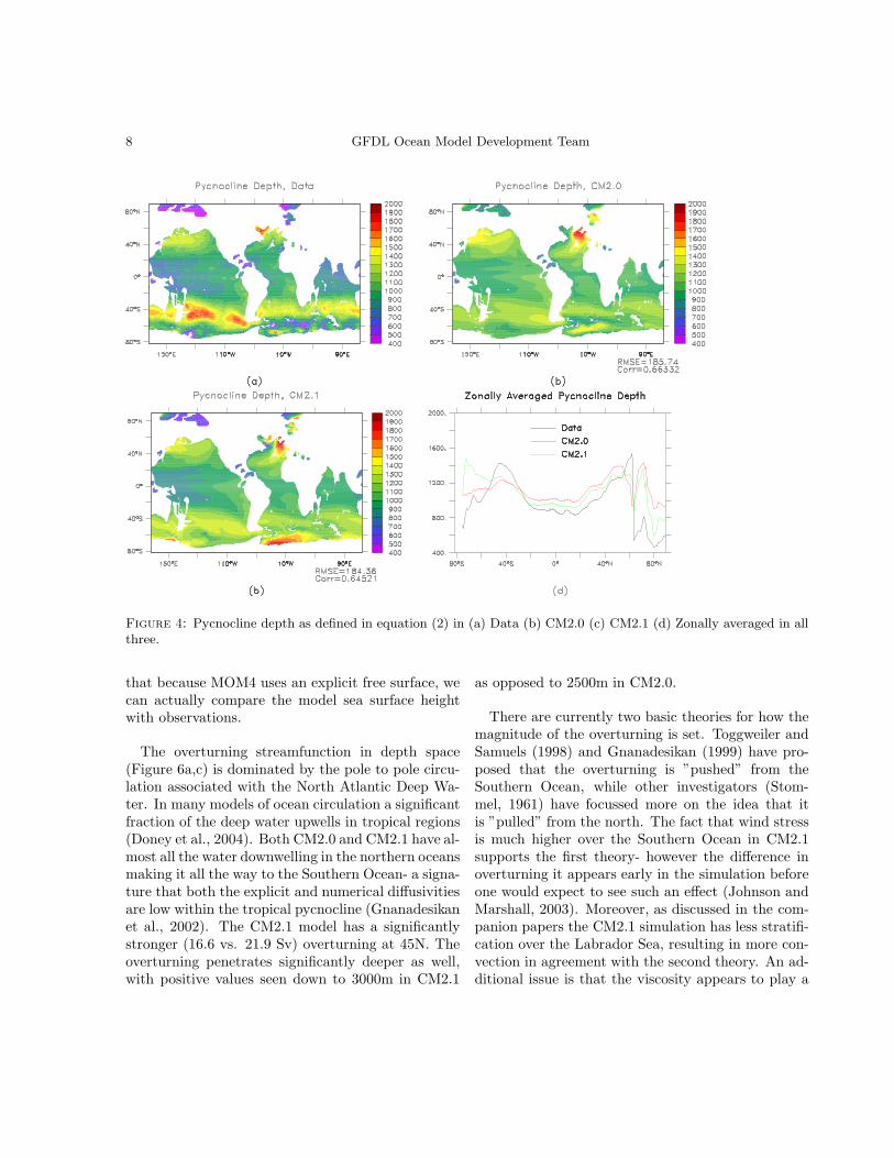
While sea surface height (compared in Figure 5with the first year of the TOPEX-Poseidon altimeter,Tapley et al., 1994) mirrors the pycnocline, the agree-ment with observations is much better. The modelcaptures the bulk of variability, with very low val-ues (less than -1.6m) in the far Southern Ocean, in-termediate values (ranging from -0.4 to 0.4m) in theAtlantic, moderately high values (0.6-0.8m) in the In-dian, and the highest values in the Pacific. The zonalaverage (Figure 5d) is extremely consistent betweenthe models and the data with the exception of thefar North Atlantic. The principal differences are as-sociated with large signals in marginal seas. We note

8 GFDL Ocean Model Development Team

Figure 4: Pycnocline depth as defined in equation (2) in (a) Data (b) CM2.0 (c) CM2.1 (d) Zonally averaged in allthree.

that because MOM4 uses an explicit free surface, wecan actually compare the model sea surface heightwith observations.

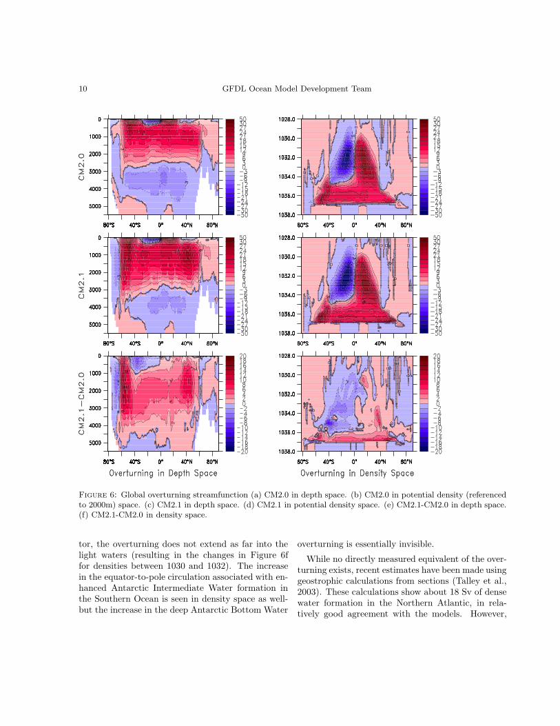
The overturning streamfunction in depth space(Figure 6a,c) is dominated by the pole to pole circu-lation associated with the North Atlantic Deep Wa-ter. In many models of ocean circulation a significantfraction of the deep water upwells in tropical regions(Doney et al., 2004). Both CM2.0 and CM2.1 have al-most all the water downwelling in the northern oceansmaking it all the way to the Southern Ocean- a signa-ture that both the explicit and numerical diffusivitiesare low within the tropical pycnocline (Gnanadesikanet al., 2002). The CM2.1 model has a significantlystronger (16.6 vs. 21.9 Sv) overturning at 45N. Theoverturning penetrates significantly deeper as well,with positive values seen down to 3000m in CM2.1

as opposed to 2500m in CM2.0.

There are currently two basic theories for how themagnitude of the overturning is set. Toggweiler andSamuels (1998) and Gnanadesikan (1999) have pro-posed that the overturning is ”pushed” from theSouthern Ocean, while other investigators (Stom-mel, 1961) have focussed more on the idea that itis ”pulled” from the north. The fact that wind stressis much higher over the Southern Ocean in CM2.1supports the first theory- however the difference inoverturning it appears early in the simulation beforeone would expect to see such an effect (Johnson andMarshall, 2003). Moreover, as discussed in the com-panion papers the CM2.1 simulation has less stratifi-cation over the Labrador Sea, resulting in more con-vection in agreement with the second theory. An ad-ditional issue is that the viscosity appears to play a

9

Figure 5: Sea surface height in (a) Data (TOPEX-Poseidon altimeter) (b) CM2.0 (c) CM2.1 (d) Zonally averagedin all three.

role in determining the rate of overturning, account-ing for about half of the change between CM2.0 andCM2.1 as discussed in more detail in Griffies et al. (inprep.). Regardless of the ultimate cause of the changein Northern Hemisphere overturning, the wind stresschanges over the Southern Ocean are likely importantin permitting this increase in overturning to connectto an increase in Southern Hemisphere upwelling.Without this increase, one would expect more adjust-ment in the density structure at depth than is seen inthese simulations. Note that the NADW circulationis not the only one that is stronger in CM2.1 thanCM2.0- the Antarctic Bottom Water Circulation isalso significantly stronger. It is not clear, however,whether this is only a transient effect.

Overturning in depth space tends to emphasize dif-ferences in deep circulations, which are quite impor-

tant for the chemical and biological properties of theocean. However, when it comes to heat transport, thesurface wind-driven circulation plays a much moreimportant role (Gnanadesikan et al., 2005, Bocalettiet al., 2005). The overturning in σ2 space (Figures6b,d) shows that most of the watermass transfor-mation crossing lines of constant density takes placein the tropics, associated with equatorial upwelling,poleward flow in the mixed layer and downwellingin somewhat surprisingly high latitudes (40 degreesin both hemispheres, i.e. the mode water forma-tion regions at the poleward edge of the subtropi-cal gyres). The somewhat stronger equatorial windsin CM2.1 have two effects on this circulation. Firstthey tend to intensify it, particularly in the South-ern Hemisphere. However, as the increased upwellingresults in a somewhat increased cold bias at the equa-

10 GFDL Ocean Model Development Team

Figure 6: Global overturning streamfunction (a) CM2.0 in depth space. (b) CM2.0 in potential density (referencedto 2000m) space. (c) CM2.1 in depth space. (d) CM2.1 in potential density space. (e) CM2.1-CM2.0 in depth space.(f) CM2.1-CM2.0 in density space.

tor, the overturning does not extend as far into thelight waters (resulting in the changes in Figure 6ffor densities between 1030 and 1032). The increasein the equator-to-pole circulation associated with en-hanced Antarctic Intermediate Water formation inthe Southern Ocean is seen in density space as well-but the increase in the deep Antarctic Bottom Water

overturning is essentially invisible.

While no directly measured equivalent of the over-turning exists, recent estimates have been made usinggeostrophic calculations from sections (Talley et al.,2003). These calculations show about 18 Sv of densewater formation in the Northern Atlantic, in rela-tively good agreement with the models. However,

11

Current name Observed CM2.0 CM2.1(Sv) (Sv) (Sv)

NADW formation 18 16.9 21.3ACC 97/134 116 132(Drake Passage)Indonesian ≈ 10 15.6 13.9ThroughflowFlorida Current 28.7-34.7 19.0 26.8Kuroshio (24N) 29-40 48.3 41.7Bering Strait 0.83 0.60 0.87EUC (155W) 24.3-35.7 38.0 34.6Atlantic DWBC (5S) 19.6-33.8 19.6 21.7Samoa Passage 3.3-8.4 -0.2 1.4

Table 1: Transports at key locations in the model.NADW formation is from Talley et al. (2003). High ob-served value of ACC at Drake Passage is from Cunning-ham et al., (2003), lower value from Orsi et al. (1995).Higher value of ACC transport is likely to be more accu-rate as it includes an (observed) barotropic component.Indonesian throughflow is from Gordon et al., (2003),Florida Current from Leaman et al. (1987), Kuroshio isfrom Lee et al. (2001), using current meters off of Taiwanand consensus estimates of flow east of the Ryukyu islands(which are not resolved in the models). Bering Strait ob-servations are from Roach et al., (1995), High value forEquatorial Undercurrent at 155W is ADCP data from theTahiti Shuttle Experiment (Lukas and Firing, 1984), lowvalue from inverse model of Sloyan et al., (2003). SamoaPassage transport is defined as net transport of water lessthan 1.2C (Johnson et al., 1994, Freeland, 2001). TheAtlantic Deep Western Boundary Current at 5S is takenfrom Rhein et al., (1995).

these calculations differ substantially from the mod-els in the Southern Ocean, where the observationalestimates have a massive formation of Antarctic Bot-tom Waters (21.8-27.3 Sv) while the models all showa significant transformation of deep waters to lighterwaters. As in many models which have low diapycnaldiffusion (Toggweiler and Samuels, 1998; Gnanade-sikan et al., 2002), our models show the SouthernOcean as a region of net lightening of surface waters.This picture is in agreement with the observationalpicture put forth by Speer et al., (2000), higher-resolution models (Hallberg and Gnanadesikan, 2005)and previously published coupled models (Doney et

al., 1998). Hallberg and Gnanadesikan (2005) suggestthat the difference between these observational syn-theses based on hydrography and the numerical mod-els may lie in the neglect of the effects of mesoscaleeddies and the strong interaction between the flowand topography.

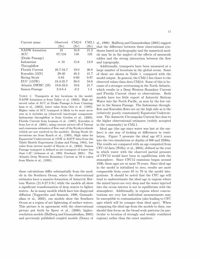
Additionally, transports have been measured at alarge number of locations in the global ocean. Someof these are shown in Table 1, compared with themodel output. In general, the CM2.1 lies closer to theobserved values than does CM2.0. Some of this is be-cause of a stronger overturning in the North Atlantic,which results in a Deep Western Boundary Currentand Florida Current closer to observations. Bothmodels have too little export of Antarctic BottomWater into the North Pacific, as seen by the low val-ues in the Samoa Passage. The Indonesian through-flow and Kuroshio flows are on the high side as is the(relatively poorly constrained) Equatorial Undercur-rent. The Antarctic Circumpolar Current lies close tothe higher observational estimates (widely acceptedin the community) in CM2.1.

Ideal age (the age since water was last at the sur-face) is one way of looking at differences in venti-lation. Figure 7 presents the ideal age 67.5 yearsinto the two simulations at depths of 800 and 2500m.The results are compared with an age computed fromCFC-12 data (Willey et al., 2004), defined as the yearin which water with the observed partial pressureof CFC12 would have been in equilibrium with theatmosphere. Since CFC12 emissions began around1930, these ages are at most 70 years. Since ideal agein the model is initialized to zero, results are mostcomparable from years 65 to 70 in the model inte-grations. It should be noted that the CFC age willtend to underestimate the ideal age in regions wherethe mixed layers are very deep and the water injectedinto the ocean interior is not in equilibrium with theatmosphere. Additionally, in regions where concen-trations are very low individual measurements maybe susceptible to contamination (also leading to CFCages which will be younger than ideal ages). Whencomparing the ideal age from the models to data, oneshould thus focus on the broad scale patterns (in par-ticular to location of strongly and weakly ventilatedregions) rather than the exact numbers.

12 GFDL Ocean Model Development Team

Figure 7: Age (a) CFC-12 age (from the dataset of Willey et al. (2004) at 800m. (b) CFC-12 age at 2500m. (c)Ideal age at 800m, CM2.0. (d) Ideal age at 2500m, CM2.0. (e) Ideal age at 800m, CM2.1. (f) Ideal age at 2500m,CM2.1.

The data shows ventilation occurring in theLabrador Sea, a band of high ventilation in the South-ern Ocean in the latitudes of the Circumpolar Cur-rent, a band of weakly ventilated water to the south(corresponding to upwelling Circumpolar Deep Wa-ter) and ventilation around the Antarctic Continent.There is also a clear signal at this depth of ventilation

in the North Pacific and a weak (though clear) signalof ventilation from the Red Sea. The boundaries ofthe poorly ventilated areas the tropical regions showup as waters older than 45 years old. These ”shadowzones” have long been known to be regions of lowoxygen are not directly ventilated from the surfacebecause their potential vorticity is too low to connect

13

with thick mixed layers in the mid-latitudes (Luytenet al., 1983). At 2500m the signal is significantlydifferent. There are two main regions of ventilation,the North Atlantic and around the Southern Ocean.Signals from the Weddell and Ross Seas can be dis-tinguished.

CM2.0 presents a picture that is qualitatively simi-lar at 800m, but quite different at 2500m. The modelrepresents most of the gross-scale features of the ven-tilation with signals from the North Atlantic, South-ern Ocean mode and intermediate waters, and NorthPacific mode water. The boundaries between recentlyventilated waters and older waters in the shadowzones are well-captured. However, there is no ven-tilation around the Antarctic boundary. This is evenmore clearly seen at 2500m, where the North AtlanticDeep Water represents the only signal of ventilation.Such a lack of ventilation has important implicationsfor the carbon cycle (Toggweiler et al., 2003; Mari-nov, 2004), implying that the venting of deep wa-ters rich in carbon dioxide is essentially capped offby stratification in the Southern Ocean.

Many, though by no means all, of the model-data differences are less pronounced in CM2.1. At800m, there is a clear banded structure in the South-ern Hemisphere, (particularly in the Atlantic sector)where one can distiguish young waters near the conti-nent, older, upwelling Circumpolar Deep Water awayfrom the continent, and young intermediate watersfurther to the north. The ventilation around the con-tinent makes it to significant depths, as seen in theideal age at 2500m. Analysis of CM2.0 and CM2.1at subsequent times shows that this difference per-sists. Although CM2.0 does occasionally ventilatethe deep waters of the Southern Ocean, such ventila-tion is much weaker than in CM2.1.

The age structure in CM2.1 also exhibits other im-provments relative to CM2.0. For example, the NorthPacific waters are clearly younger at 800m in CM2.1.In the North Atlantic there is a clear signal of convec-tion in the Labrador Sea, implications of which arediscussed in more depth in the companion paper byStouffer et al. (this volume). However, there are cer-tain features (excessive ventilation in the NortheastAtlantic, lack of ventilation in the Red Sea) that donot change between the models.

4 Regional diagnostics

a. Southern Hemisphere

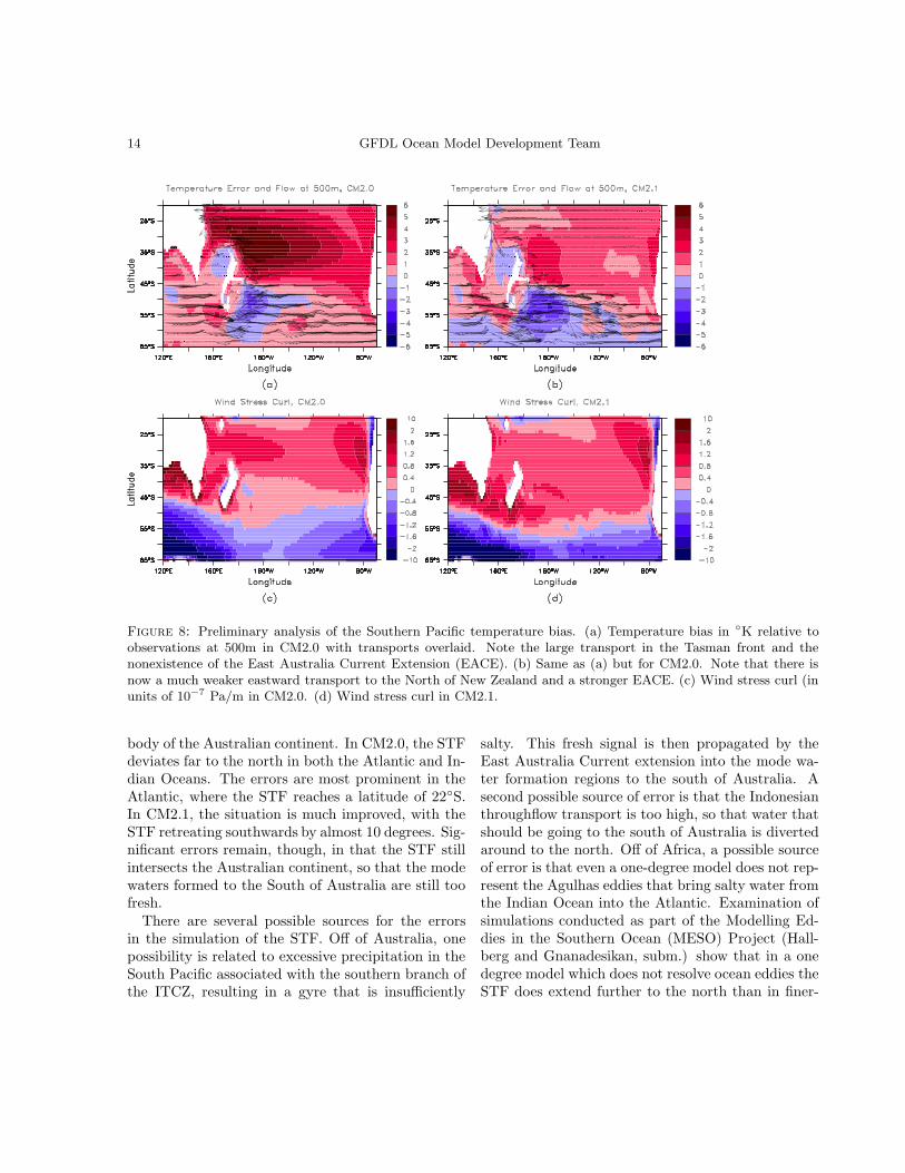
Since it has already been shown that the largest dif-ferences in temperature and salinity errors betweenthe models occur in the Southern hemisphere, we be-gin our analysis in this region. One of the strikingdifferences between CM2.0 and CM2.1 is the differ-ence in the RMS temperature error seen in Figure3a and b. Interestingly, the largest errors in CM2.0do not show up at the surface, but rather reach theirmaximum at a depth of around 500m. Figure 8 showsa closeup of the temperature error and circulation at500m in the two models. Observations (Ridgewayand Dunn, 2003) and high-resolution numerical mod-els (Tilburg et al., 2001) suggest that the real EastAustralia Current splits at a latitude of 30S with theTasman front striking off to the east and the EastAustralia Current extension continuing to the south.In CM2.0, the East Australia Current extension es-sentially feeds all its transport into the Tasman front,carrying warm subtropical water deep into the SouthCentral Pacific. In CM2.1 by contrast the East Aus-tralia current continues to the south, and feeds theFlinders Current south of Tasmania.

The difference between the two circulations canlargely be explained in terms of the wind stress curl.In CM2.0 strong positive wind stress curl is onlyfound northwards of 42-44◦ S in the South Pacific,so that the bulk of the subtropical gyre lies to thenorth of New Zealand. In CM2.1 the wind stress curlbetween New Zealand and South America remainspositive down to 55◦S, so that all of New Zealandlies within the Subtropical Gyre. Russell et al. (inprep.) discuss this issue in more detail.

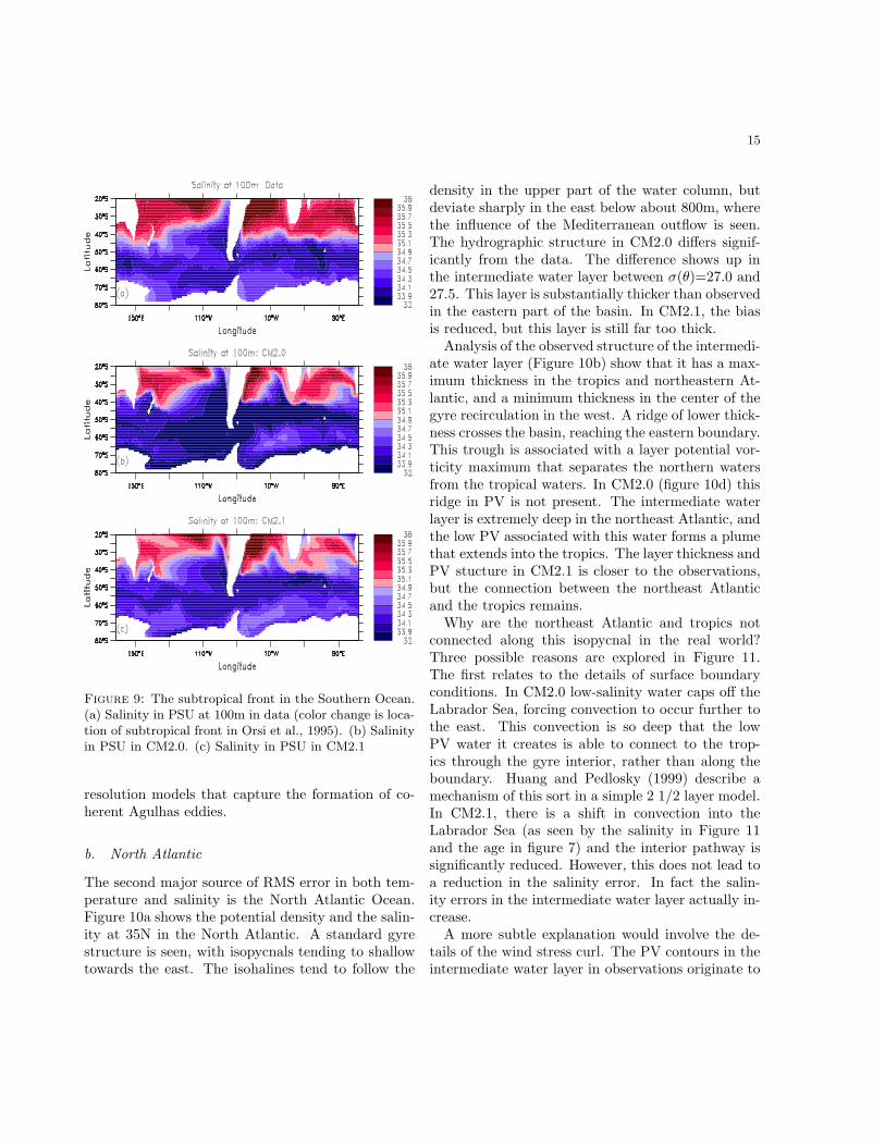
The big improvement in RMS salinity error be-tween CM2.0 and CM2.1 is seen in the South AtlanticOcean. The source of the error is the position of thesubtropical front (STF). Figure 9 shows the locationof the subtropical front (defined, as in Orsi et al.,(1995) as where the 34.9 isohaline surface is found ata depth of 100m). In the observations, the subtropi-cal front crosses the South Atlantic and South IndianOceans between the latitudes of 36◦S and 40◦S, wellto the south of the Cape of Good Hope and the main

14 GFDL Ocean Model Development Team

� � �

�

�

�

���

�

�

�

�

�

�

� �

�

� �

�

�

�

�

�

�

�

�

�

�

�

�

�

�

�

�

�

�

�

�

�

�

�

�

�

�

�

�

�

�

�

�

�

�

�

�

�

�

�

�

�

�

�

�

�

�

�

�

�

�

�

�

�

�

�

�

�

� � � �

�

�

�

�

�

�

�

�

�

�

�

�

�

�

�

�

Figure 8: Preliminary analysis of the Southern Pacific temperature bias. (a) Temperature bias in ◦K relative toobservations at 500m in CM2.0 with transports overlaid. Note the large transport in the Tasman front and thenonexistence of the East Australia Current Extension (EACE). (b) Same as (a) but for CM2.0. Note that there isnow a much weaker eastward transport to the North of New Zealand and a stronger EACE. (c) Wind stress curl (inunits of 10−7 Pa/m in CM2.0. (d) Wind stress curl in CM2.1.

body of the Australian continent. In CM2.0, the STFdeviates far to the north in both the Atlantic and In-dian Oceans. The errors are most prominent in theAtlantic, where the STF reaches a latitude of 22◦S.In CM2.1, the situation is much improved, with theSTF retreating southwards by almost 10 degrees. Sig-nificant errors remain, though, in that the STF stillintersects the Australian continent, so that the modewaters formed to the South of Australia are still toofresh.

There are several possible sources for the errorsin the simulation of the STF. Off of Australia, onepossibility is related to excessive precipitation in theSouth Pacific associated with the southern branch ofthe ITCZ, resulting in a gyre that is insufficiently

salty. This fresh signal is then propagated by theEast Australia Current extension into the mode wa-ter formation regions to the south of Australia. Asecond possible source of error is that the Indonesianthroughflow transport is too high, so that water thatshould be going to the south of Australia is divertedaround to the north. Off of Africa, a possible sourceof error is that even a one-degree model does not rep-resent the Agulhas eddies that bring salty water fromthe Indian Ocean into the Atlantic. Examination ofsimulations conducted as part of the Modelling Ed-dies in the Southern Ocean (MESO) Project (Hall-berg and Gnanadesikan, subm.) show that in a onedegree model which does not resolve ocean eddies theSTF does extend further to the north than in finer-

15

Figure 9: The subtropical front in the Southern Ocean.(a) Salinity in PSU at 100m in data (color change is loca-tion of subtropical front in Orsi et al., 1995). (b) Salinityin PSU in CM2.0. (c) Salinity in PSU in CM2.1

resolution models that capture the formation of co-herent Agulhas eddies.

b. North Atlantic

The second major source of RMS error in both tem-perature and salinity is the North Atlantic Ocean.Figure 10a shows the potential density and the salin-ity at 35N in the North Atlantic. A standard gyrestructure is seen, with isopycnals tending to shallowtowards the east. The isohalines tend to follow the

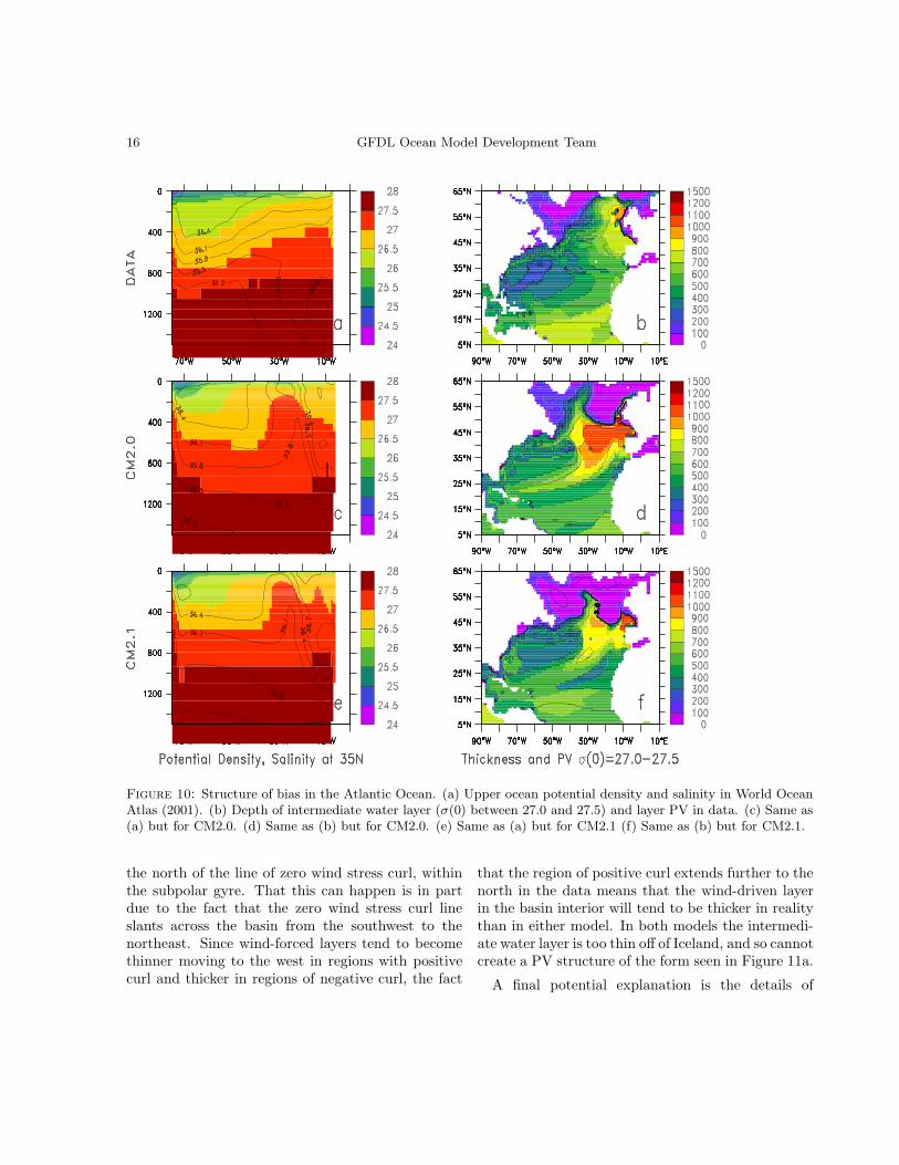
density in the upper part of the water column, butdeviate sharply in the east below about 800m, wherethe influence of the Mediterranean outflow is seen.The hydrographic structure in CM2.0 differs signif-icantly from the data. The difference shows up inthe intermediate water layer between σ(θ)=27.0 and27.5. This layer is substantially thicker than observedin the eastern part of the basin. In CM2.1, the biasis reduced, but this layer is still far too thick.

Analysis of the observed structure of the intermedi-ate water layer (Figure 10b) show that it has a max-imum thickness in the tropics and northeastern At-lantic, and a minimum thickness in the center of thegyre recirculation in the west. A ridge of lower thick-ness crosses the basin, reaching the eastern boundary.This trough is associated with a layer potential vor-ticity maximum that separates the northern watersfrom the tropical waters. In CM2.0 (figure 10d) thisridge in PV is not present. The intermediate waterlayer is extremely deep in the northeast Atlantic, andthe low PV associated with this water forms a plumethat extends into the tropics. The layer thickness andPV stucture in CM2.1 is closer to the observations,but the connection between the northeast Atlanticand the tropics remains.

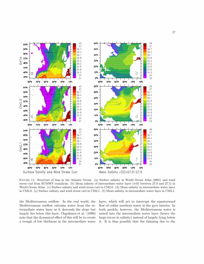
Why are the northeast Atlantic and tropics notconnected along this isopycnal in the real world?Three possible reasons are explored in Figure 11.The first relates to the details of surface boundaryconditions. In CM2.0 low-salinity water caps off theLabrador Sea, forcing convection to occur further tothe east. This convection is so deep that the lowPV water it creates is able to connect to the trop-ics through the gyre interior, rather than along theboundary. Huang and Pedlosky (1999) describe amechanism of this sort in a simple 2 1/2 layer model.In CM2.1, there is a shift in convection into theLabrador Sea (as seen by the salinity in Figure 11and the age in figure 7) and the interior pathway issignificantly reduced. However, this does not lead toa reduction in the salinity error. In fact the salin-ity errors in the intermediate water layer actually in-crease.

A more subtle explanation would involve the de-tails of the wind stress curl. The PV contours in theintermediate water layer in observations originate to

16 GFDL Ocean Model Development Team

Figure 10: Structure of bias in the Atlantic Ocean. (a) Upper ocean potential density and salinity in World OceanAtlas (2001). (b) Depth of intermediate water layer (σ(0) between 27.0 and 27.5) and layer PV in data. (c) Same as(a) but for CM2.0. (d) Same as (b) but for CM2.0. (e) Same as (a) but for CM2.1 (f) Same as (b) but for CM2.1.

the north of the line of zero wind stress curl, withinthe subpolar gyre. That this can happen is in partdue to the fact that the zero wind stress curl lineslants across the basin from the southwest to thenortheast. Since wind-forced layers tend to becomethinner moving to the west in regions with positivecurl and thicker in regions of negative curl, the fact

that the region of positive curl extends further to thenorth in the data means that the wind-driven layerin the basin interior will tend to be thicker in realitythan in either model. In both models the intermedi-ate water layer is too thin off of Iceland, and so cannotcreate a PV structure of the form seen in Figure 11a.

A final potential explanation is the details of

17

Figure 11: Structure of bias in the Atlantic Ocean. (a) Surface salinity in World Ocean Atlas (2001) and windstress curl from ECMWF reanalysis. (b) Mean salinity of intermediate water layer (σ(0) between 27.0 and 27.5) inWorld Ocean Atlas. (c) Surface salinity and wind stress curl in CM2.0. (d) Mean salinity in intermediate water layerin CM2.0. (e) Surface salinity and wind stress curl in CM2.1. (f) Mean salinity in intermediate water layer in CM2.1.

the Mediterranean outflow. In the real world, theMediterranean outflow entrains water from the in-termediate water layer as it descends the slope butlargely lies below this layer. Ozgokmen et al. (1999)note that the dynamical effect of this will be to createa trough of low thickness in the intermediate water

layer, which will act to interrupt the equatorwardflow of colder northern water in the gyre interior. Inboth models, however, the Mediterranean water ismixed into the intermediate water layer (hence thelarge errors in salinity) instead of largely lying belowit. It is thus possible that the thinning due to the

18 GFDL Ocean Model Development Team

Mediterranean beta-plume is underestimated.

c. North Pacific

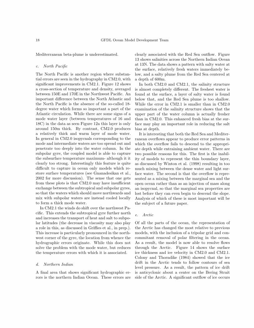
The North Pacific is another region where substan-tial errors are seen in the hydrography in CM2.0, withsignificant improvements in CM2.1. Figure 12 showsa cross-section of temperature and density, averagedbetween 150E and 170E in the Northwest Pacific. Animportant difference between the North Atlantic andthe North Pacific is the absence of the so-called 18-degree water which forms so important a part of theAtlantic circulation. While there are some signs of amode water layer (between temperatures of 16 and18C) in the data as seen Figure 12a this layer is onlyaround 150m thick. By contrast, CM2.0 producesa relatively thick and warm layer of mode water.In general in CM2.0 isopycnals corresponding to themode and intermediate waters are too spread out andpenetrate too deeply into the water column. In thesubpolar gyre, the coupled model is able to capturethe subsurface temperature maximum- although it itclearly too strong. Interestingly this feature is quitedifficult to capture in ocean only models which re-store surface temperatures (see Gnanadesikan et al.,2002 for more discussion). The sense that one getsfrom these plots is that CM2.0 may have insufficientexchange between the subtropical and subpolar gyres,so that the waters which should move northwards andmix with subpolar waters are instead cooled locallyto form a thick mode water.

In CM2.1 the winds do shift over the northwest Pa-cific. This extends the subtropical gyre further northand increases the transport of heat and salt to subpo-lar latitudes (the decrease in viscosity may also playa role in this, as discussed in Griffies et al., in prep.).This increase is particularly pronounced in the north-west corner of the gyre, the location from whence thehydrographic errors originate. While this does notsolve the problem with the mode water, but reducesthe temperature errors with which it is associated.

d. Northern Indian

A final area that shows significant hydrographic er-rors is the northern Indian Ocean. These errors are

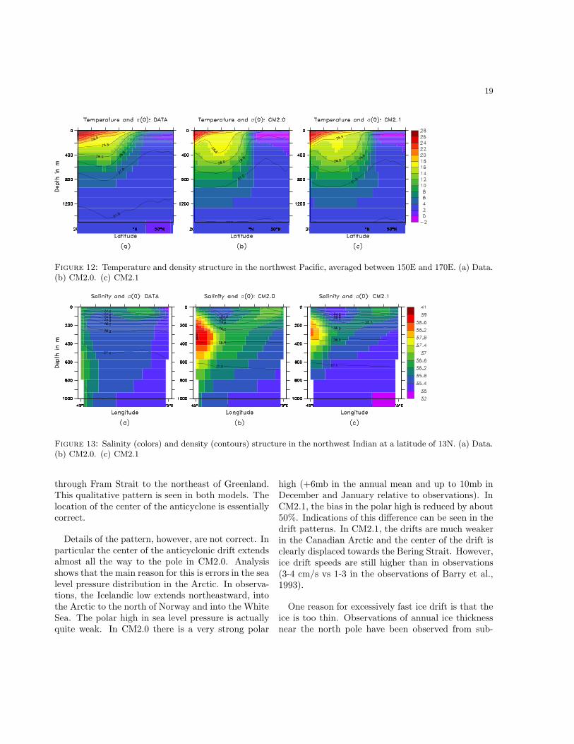
clearly associated with the Red Sea outflow. Figure13 shows salinities across the Northern Indian Oceanat 13N. The data shows a pattern with salty water atthe surface, relatively fresh waters immediately be-low, and a salty plume from the Red Sea centered ata depth of 600m.

In both CM2.0 and CM2.1, the salinity structureis almost completely different. The freshest water isfound at the surface, a layer of salty water is foundbelow that, and the Red Sea plume is too shallow.While the error in CM2.1 is smaller than in CM2.0examination of the salinity structure shows that theupper part of the water column is actually fresherthan in CM2.0. This enhanced fresh bias at the sur-face may play an important role in reducing the saltbias at depth.

It is interesting that both the Red Sea and Mediter-ranean overflows appear to produce error patterns inwhich the overflow fails to descend to the appropri-ate depth while entraining ambient water. There aretwo possible reasons for this. The first is the inabil-ity of models to represent the thin boundary layer,as discussed by Winton et al. (1998) resulting in toomuch mixing between the dense water and light sur-face water. The second is that the overflow is repre-sented as a mixing between the marginal sea and theopen ocean rather than as an injection of mass alongan isopycnal, so that the marginal sea properties arelost before they can even begin to descend the slope.Analysis of which of these is most important will bethe subject of a future paper.

e. Arctic

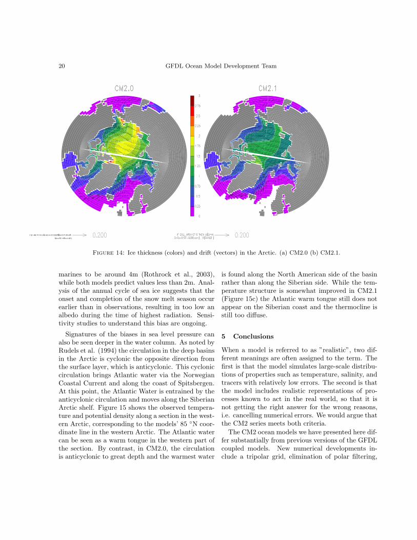
Of all the parts of the ocean, the representation ofthe Arctic has changed the most relative to previousmodels, with the inclusion of a tripolar grid and con-commitant removal of polar filtering in the ocean.As a result, the model is now able to resolve flowsthrough the Arctic. Figure 14 shows the surfaceice thickness and ice velocity in CM2.0 and CM2.1.Colony and Thorndike (1984) showed that the icedrift in the Arctic tends to follow contours of sealevel pressure. As a result, the pattern of ice driftis anticyclonic about a center on the Bering Straitside of the Arctic. A significant outflow of ice occurs

19

Figure 12: Temperature and density structure in the northwest Pacific, averaged between 150E and 170E. (a) Data.(b) CM2.0. (c) CM2.1

Figure 13: Salinity (colors) and density (contours) structure in the northwest Indian at a latitude of 13N. (a) Data.(b) CM2.0. (c) CM2.1

through Fram Strait to the northeast of Greenland.This qualitative pattern is seen in both models. Thelocation of the center of the anticyclone is essentiallycorrect.

Details of the pattern, however, are not correct. Inparticular the center of the anticyclonic drift extendsalmost all the way to the pole in CM2.0. Analysisshows that the main reason for this is errors in the sealevel pressure distribution in the Arctic. In observa-tions, the Icelandic low extends northeastward, intothe Arctic to the north of Norway and into the WhiteSea. The polar high in sea level pressure is actuallyquite weak. In CM2.0 there is a very strong polar

high (+6mb in the annual mean and up to 10mb inDecember and January relative to observations). InCM2.1, the bias in the polar high is reduced by about50%. Indications of this difference can be seen in thedrift patterns. In CM2.1, the drifts are much weakerin the Canadian Arctic and the center of the drift isclearly displaced towards the Bering Strait. However,ice drift speeds are still higher than in observations(3-4 cm/s vs 1-3 in the observations of Barry et al.,1993).

One reason for excessively fast ice drift is that theice is too thin. Observations of annual ice thicknessnear the north pole have been observed from sub-

20 GFDL Ocean Model Development Team

Figure 14: Ice thickness (colors) and drift (vectors) in the Arctic. (a) CM2.0 (b) CM2.1.

marines to be around 4m (Rothrock et al., 2003),while both models predict values less than 2m. Anal-ysis of the annual cycle of sea ice suggests that theonset and completion of the snow melt season occurearlier than in observations, resulting in too low analbedo during the time of highest radiation. Sensi-tivity studies to understand this bias are ongoing.

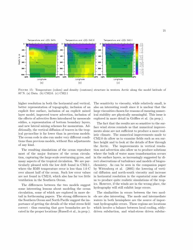
Signatures of the biases in sea level pressure canalso be seen deeper in the water column. As noted byRudels et al. (1994) the circulation in the deep basinsin the Arctic is cyclonic the opposite direction fromthe surface layer, which is anticyclonic. This cycloniccirculation brings Atlantic water via the NorwegianCoastal Current and along the coast of Spitsbergen.At this point, the Atlantic Water is entrained by theanticyclonic circulation and moves along the SiberianArctic shelf. Figure 15 shows the observed tempera-ture and potential density along a section in the west-ern Arctic, corresponding to the models’ 85 ◦N coor-dinate line in the western Arctic. The Atlantic watercan be seen as a warm tongue in the western part ofthe section. By contrast, in CM2.0, the circulationis anticyclonic to great depth and the warmest water

is found along the North American side of the basinrather than along the Siberian side. While the tem-perature structure is somewhat improved in CM2.1(Figure 15c) the Atlantic warm tongue still does notappear on the Siberian coast and the thermocline isstill too diffuse.

5 Conclusions

When a model is referred to as ”realistic”, two dif-ferent meanings are often assigned to the term. Thefirst is that the model simulates large-scale distribu-tions of properties such as temperature, salinity, andtracers with relatively low errors. The second is thatthe model includes realistic representations of pro-cesses known to act in the real world, so that it isnot getting the right answer for the wrong reasons,i.e. cancelling numerical errors. We would argue thatthe CM2 series meets both criteria.

The CM2 ocean models we have presented here dif-fer substantially from previous versions of the GFDLcoupled models. New numerical developments in-clude a tripolar grid, elimination of polar filtering,

21

Figure 15: Temperature (colors) and density (contours) structure in western Arctic along the model latitude of85◦N. (a) Data. (b) CM2.0. (c) CM2.1

higher resolution in both the horizontal and vertical,better representation of topography, inclusion of anexplicit free surface, inclusion of an explicit mixedlayer model, improved tracer advection, inclusion ofthe effects of advective flows introduced by mesoscaleeddies, a representation of bottom boundary layers,and new lateral mixing schemes for momentum. Ad-ditionally, the vertical diffusion of tracers in the trop-ical pycnocline is far lower than in previous models.The ocean code is also run under very different condi-tions than previous models, without flux adjustmentsof any kind.

The resulting simulations of the ocean reproducemost of the major features of the ocean circula-tion, capturing the large-scale overturning gyres, andmany aspects of the tropical circulation. We are par-ticularly pleased with the low drift found in CM2.1,where the RMS temperature error is less than 1.0 Cover almost half of the ocean. Such low error valuesare not found in CM2.0, which also has far too littleventilation in the Southern Ocean.

The differences between the two models suggestsome interesting lessons about modeling the oceancirculation, some of which are explored in more de-tail in forthcoming papers. The strong differences inthe Southern Ocean and North Pacific suggest the im-portance of getting the details of the wind stress fieldcorrect - thus ensuring that gyre boundaries are lo-cated in the proper locations (Russell et al., in prep.).

The sensitivity to viscosity, while relatively small, isalso an interesting result since it is unclear that thelarge viscosities chosen for reasons of ensuring numer-ical stability are physically meaningful. This issue isexplored in more detail in Griffies et al. (in prep.).

The fact that the results are so sensitive to the sur-face wind stress reminds us that numerical improve-ments alone are not sufficient to produce a more real-istic climate. The numerical improvements made toCM2.0 do allow us to examine fields such as sea sur-face height and to look at the details of flow throughthe Arctic. The improvements in vertical resolu-tion and advection also allow us to produce solutionswhere the bulk of water mass transformation occursin the surface layers, as increasingly suggested by di-rect observations of turbulence and models of biogeo-chemistry. As can be seen in the companion paperby Wittenberg et al. (2005) the lowering of verti-cal diffusion and north-south viscosity and increasein horizontal resolution in the equatorial zone allowus to produce quite realistic simulations of the trop-ics. However, if the winds are in the wrong place, thehydrography will still exhibit large errors.

The similarities in errors between the two mod-els are also interesting. The mode and intermediatewaters in both hemisphere are the source of impor-tant hydrographic errors. These regions are locationswhich involve a balance between local cooling, eddy-driven subduction, and wind-stress driven subduc-

22 GFDL Ocean Model Development Team

tion. Additionally, both models have significant er-rors in hydrographic structure in both the Mediter-ranean Sea and northern Indian Ocean, which ap-pear to be associated with the representation of denseoverflows. The similarities in these errors in particu-lar point to overflows as a key process which can beimproved in future generations of the ocean model.

Acknowledgments

We would like to thank the entire laboratory, es-pecially our director Ants Leetmaa, for making avail-able the support and computational resources to com-plete this model. We thank Robbie Toggweiler andSonya Legg for their reviews of this paper, and Ge-off Vallis, Bob Hallberg, Alistair Adcroft, and BrianArbic for useful discussions during the developmentprocess. Chloroflourocarbon data was made availablethrough the GLODAP Project.

23

References

Adcroft, A., C. Hill and J. Marshall, 1997: Rep-resentation of topography by shaved cells ina height coordinate ocean model, Mon. Wea.

Rev., 125, 2293-2315.

Barry, R.G., M.C. Serreze, J.A. Maslanik, and R.H.Preller, 1993: The Arctic sea ice-climate system:Observations and modeling, Rev. Geophys., 31,397-422.

Beckman, A. and R. Doscher, 1997: A method forimproved representation of dense water spread-ing over topography in geopotential-coordinatemodels, J. Phys. Oceanogr., 27, 581-591.

Bocaletti,G., R. Ferrari, A. Adcroft and J. Marshall,2005: The vertical structure of ocean heat trans-port, subm. manuscript.

Bryan, K, and L.J. Lewis, 1979: A water massmodel of the world ocean, J. Geophys. Res., 84,2503-2517.

Colony, R.L. and A.S. Thorndike, 1984: An estimateof the mean field of Arctic sea ice motion, J.

Geophys. Res., 89, 623-629.

Cunningham, S.A., S.G. Alderson, B.A. King andM.A. Brandon, 2003: Transport and variabilityof the Antarctic Circumpolar Current in DrakePassage, J. Geophys. Res., 108, Art. 8084.

Delworth, T. L., R. J. Stouffer, K. W. Dixon, M.J. Spelman, T. R. Knutson, A. J. Broccoli, P.J. Kushner, and R. T. Wetherald, 2002: Reviewof simulations of climate variability and changewith the GFDL R30 coupled climate model. Cli-

mate Dynamics, 19, 555-574.

Delworth, T., et al., 2005: GFDL’s CM2 CoupledClimate Models: Part I- Formulation and simu-lation characteristics, subm. J. Climate.

Doney, S.C., W.G. Large and F.O. Bryan, 1998:Surface ocean fluxes and water-mass transforma-tion rates in the coupled NCAR Climate SystemModel, J. Clim., 11, 1420-1441.

Doney, S.C., et al., 2004: Evaluating global oceancarbon models: The importance of realisticphysics, Global Biogeochem. Cyc., 18, GB3017,doi:10.1029/2003GB002150.

Freeland, J., 2001: Observations of the flow ofabyssal water through the Samoa Passage, J.

Phys. Oceanogr., 31, 2283-2279.

Gent, P. and J.C. McWilliams, 1990: Isopycnalmixing in ocean circulation models, J. Phys.

Oceanogr., 20, 150-155.

Gnanadesikan, A., 1999: A simple predictive modelfor the structure of the oceanic pycnocline, Sci-

ence, 283, 2077-2079.

Gnanadesikan, A., R.D. Slater, N. Gruber andJ.L. Sarmiento, 2002: Oceanic vertical exchangeand new production: A model-data comparison,Deep Sea Res. II, 43, 363-401.

Gnanadesikan, A., R.D. Slater, P.S. Swathi andG.K. Vallis, 2005: The energetics of ocean heattransport, subm. J. Climate.

Gordon, A.L., R.D. Susanto and K. Vranes, 2003:Cool Indonesian throughflow as a consequenceof restricted surface layer flow, Nature, 425, 824-828, doi:10.1038/nature02038.

Griffies, S.M., 1998: The Gent-McWilliams skew-flux, J. Phys. Oceanogr., 28, 831-841.

Griffies, S.M., A. Gnanadesikan, R.C. Pacanowski,V.D. Larichev, J.K. Dukowicz, and R.D. Smith,1998: Isopycnal mixing in a z-coordinate oceanmodel, J. Phys. Oceanogr., 28, 805-830.

Griffies, S.M., R. C. Pacanowski and R.W. Hallberg,2000: Spurious diapycnal mixing associated withadvection in a z-coordinate ocean model, Mon.

Wea. Rev., 128, 538-564.

Griffies, S.M., R.C. Pacanowski, R.M. Schmidt, andV. Balaji, 2001: Tracer conservation with an ex-plicit free surface m,ethod for z-coordinate oceanmodels, Mon. Wea. Rev., 129, 1081-1098.

24 GFDL Ocean Model Development Team

Griffies, S.M., et al., 2005: Formulation of an oceanmodel for a coupled climate simulation, in prep.,Ocean Modelling.

Hallberg, R.W., and A. Gnanadesikan, 2005: Therole of eddies in determining the structure andresponse of the wind-driven Southern Hemi-sphere overturning: Initial results from the Mod-eling Eddies in the Southern Ocean Project.,subm. J. Phys. Oceanogr..

Huang, R.X. and J. Pedlosky, 2000: Climate vari-ability induced by anomalous buoyancy forcingin a multilayer model of the ventilated thermo-cline, J. Phys. Oceanogr., 30, 3009-3021.

Hundsdorfer, W. and R. Trompert, 1994: Method oflines and direct discretization: a comparison forlinear advection, Appl. Num. Math., 469-490.

Johnson, G.C., D.L. Rudnick and B.A. Taft, 1994:Bottom water variability in the Samoa Passage,Deep Sea Res., 52, 177-196.

Johnson, H.L., D.P. Marshall, 2004: Global tele-connections of meridional overturning circula-tion anomalies, J. Phys. Oceanogr., 34, 1702-1722.

Large, W., G. Danasbogulu, J.C. McWilliams, P.R.Gent, and F.O. Bryan, 2001: Equatorial cir-culation of a global ocean climate model withanisotropic viscosity, J. Phys. Oceanogr., 31,518-536.

Large, W., J.C. McWilliams, and S.C. Doney, 1994:Oceanic vertical mixing: A review and a modelwith a nonlocal boundary mixing parameteriza-tion, Rev. Geophys., 32, 363-403.

Leaman, K.D., R.L. Molinari, P.S. Vertes, 1987:Structure and variability of the Florida Cur-rent at 27N: April 1982- July 1984, J. Phys.

Oceanogr., 17, 565-583.

Ledwell, J.R., A.J. Watson, and C.S. Law, 1993:Evidence for slow mixing across the pycnoclinefrom an open-ocean tracer-release experiment,Nature, 364, 701-703.

Ledwell, J.R., A.J. Watson, and C.S. Law, 1998:Mixing of a tracer in the pycnocline, J. Geophys.

Res.,103, 21499-21530.

Lee, T.N., W.E. Johns, C.T. Liu, D. Zhand, R. Zan-topp, Y.Yang, 2001: Mean transport and sea-sonal cycle of the Kuroshio east of Taiwan withcomparison to the Florida Current, J. Geophys.

Res., 106, 22143-22158.

Lee, H.-C., A. Rosati, M. Spelman and T. Delworth,2005: Barotropic tidal mixing impact in a cou-pled climate model: ocean condition and merid-ional overturning circulation in the the northernAtlantic, in prep.

Levine,M.D., C.A. Paulson and J.H. Morison, 1984:Internal waves in the Arctic Ocean: Compar-ison with lower-latitude observations, J. Phys.

Oceanogr., 15, 800-809.

Lukas, R., and E. Firing, 1984: The geostrophicbalance of the Pacific equatorial undercurrent,Deep Sea Res., 31, 61-66.

Luyten, J.R., J. Pedlosky, H. Stommel, 1983: Theventilated thermocline, J. Phys. Oceanogr., 13,292-309.

Manabe, S. and K. Bryan, 1969: Climate calcua-tions with a combined ocean-atmosphere model,J. Atmos. Sci., 26, 786-789.

Manabe, S., R. Stouffer, M. Spelman and K. Bryan,1991: Transient responses of a coupled ocean-atmosphere model to gradual changes of atmo-sphere CO2. Part 1: Annual mean response, J.

of Climate, 4, 785-818.

Marinov, I., 2004: Controls on the air-sea balance ofCO2, Ph.D. Dissertation, Princeton University.

Matsumoto, K., et al., 2004: Evaluation ofocean carbon cycle models with data-basedmetrics, Geophys. Res. Lett., 31, L07303,doi:10.1029/2003GL018970.

Morel, A. and D. Antoine, 1994: Heating rate withinthe upper ocean in relation to its bio-opticalstate, J. Phys. Oceanogr., 24, 1652-1665.

25

Murray, R.J., 1996: Explicit generation of orthog-onal grids for ocean models, J. Comput. Phys.,126, 251-273.

Orsi, A.H., T. Whitworth and W.D. Nowlin, 1995:On the meridional extent and fronts of theAntarctic Circumpolar Current, Deep Sea Res.

I, 42, 641-673.

Ozgokmen, T.M., E.P. Chassignet and C.G.H.Rooth, 2001: On the connection between theMediterranean Outflow and the Azores Current,J. Phys. Oceanogr., 31, 461-480.

Pacanowski, R.C. and A. Gnanadesikan, 1998:Transient response in a z-level ocean modelthat resolves topography with partial cells, Mon.

Wea. Rev., 126, 3248-3270.

Park, Y.-G. and K. Bryan, 2000: Comparisonof thermally-driven circulations from a depth-coordinate model and an isopycnal-layer model.Part 1: Scaling-law sensitivity to vertical diffu-sivity, J. Phys. Oceanogr., 30, 590-605.

Polzin, K., 1999: A rough recipe for the energybalance of quasi-steady lee waves, ’Aha Huliko’a

Winter Workshop: Dynamics of internal gravity

waves II, 117-128.

Polzin, K., J.M. Toole, J.R. Ledwell and R.W.Schmitt, 1997: Spatial variability of turbulentmixing in the abyssal ocean, Science, 276, 93-96.

Rhein, M., L. Stramma, U. Send, 1995: The At-lantic Deep Western Boundary Current: Watermasses and transports near the equator, J. Geo-

phys. Res., 100, 2441-2457.

Rhines, P.B. and W.R. Young, 1982: Potentialvorticity homogenization in planetary gyres, J.

Fluid Mech., 122, 347-367.

Ridgway, K.R. and J.R. Dunn, 2003: Mesoscalestructure of the mean East Australian CurrentSystem and its relationship with topography,Prog. Oceanogr., 56, 189-222.

Roach,A.T., K. Aagard, C.H. Pease, S.A. Salo,T. Weingartner, V. Pavlov, M. Kulakov, 1995:Direct measurements of transport and waterproperties through Bering Strait, J. Geophys.

Res.,100, 18443-18457

Rudels, B., E.P. Jones, L.G. Anderson and G. Kat-tner, 1994: On the intermediate depth waters ofthe Arctic Ocean, in The Polar Oceans and their

role in shaping the global environment, O.M. Jo-hannsessen, R.D. Muench and J.E. Overland,(eds.), Geophysical Monograph, 85, AmericanGeophysical Union, Washington, DC, 33-46.

Russell, J.E., A. Gnanadesikan and J.R. Toggweiler,in prep., Impact of the annular mode on the cir-culation of the Southern Ocean, in prep.

Sarmiento, J.L., T.M.C. Hughes, R.J. Stouffer, andS. Manabe, 1998: Ocean carbon cycle responseto future greenhouse warming, Nature, 393, 245-249.

Simmons, H.L., S.R. Jayne, L.C. St. Laurent, andA.J. Weaver, 2004: Tidally driven mixing in anumerical model of the ocean general circulation,Ocean Modelling, 6, 245-263.

Sloyan, B.M., G.C. Johnson and W.S. Kessler, 2003:The Pacific Cold Tongue: A pathway for inter-hemispheric exchange, J. Phys. Oceanogr., 33,1027-1043.

Speer, K.G., S.R. Rintoul and B. Sloyan, 2000: Thediabatic Deacon Cell, J. Phys. Oceanogr., 30,3212-3222.

Stommel, H., 1961: Thermohaline convection withtwo stable regimes of flow, Tellus, 13, 224-228.

Stouffer, R.J., 2004: Time scales of climate re-sponse, J. Clim., 17, 209-217.

Stouffer, R.J., et al., 2005: GFDL’s CM2 coupledclimate models- Part 4: Idealized climate re-sponse, subm. J. Climate

Sweby, P., 1984: High-resolution schemes using fluxlimiters for hyperbolic conservation laws, SIAM

J. Num. Anal., 21, 995-1011.

26 GFDL Ocean Model Development Team

Sweeney, C., A. Gnanadesikan, S.M. Griffies, M.Harrison, A. Rosati and B. Samuels, 2004: Im-pacts of shortwave penetration depth on large-scale ocean circulation and heat transport, J.

Phys. Oceanogr., in press.

Talley, L.D., J.L. Reid and P.E. Robbins, 2003:Data-based meridional overturning streamfunc-tions for the Global Ocean, J. Climate 16, 3213-3226.

Tapley, B.D., D.P. Chambers, C.K. Shum, R.J.Eanes, J.C. Ries and R.H. Stewart, 1994: Accu-racy assessment of the large-scale dynamic oceantopography from TOPEX/Poseidon altimetry,J. Geophys. Res., 99 (C12), 24605-24617.

Tilburg, C.E., H.E. Hurlburt, J.J. O’Brien and J.F.Shriver, 2001: The dynamics of the East Aus-tralia Current system: The Tasman Front, theEast Auckland Current, and the East Cape Cur-rent, J. Phys. Oceanogr., 31, 2917-2943.

Toggweiler, J.R., and B. Samuels, 1998: On theocean’s large-scale circulation near the limit ofno vertical mixing, J. Phys. Oceanogr., 28,1832-1852.

Toggweiler, J.R., R. Murnane, S. Carson, A.Gnanadesikan and J.L. Sarmiento, 2003: Repre-sentation of the carbon cycle in box models andGCMs: 2. Organic pump, Global Biogeochem.

Cyc., 17, doi:10.1029/2001GB001841.

Willey, D.A., R.A. Fine, R.E. Sonnerup, J.L.Bullister, W.M. Smethie, and M.J. Warner,2004: Global oceanic chloroflourocarbon in-ventory, Geophys. Res. Lett., 31, L1303,doi:10.1029/2003GL018816.

Winton, M., 2003: On the climatic impact of oceancirculation, J. Clim., 16, 2875-2889.

Winton, M., R.W. Hallberg, and A. Gnanadesikan,1998: Simulation of density-driven frictionaldownslope flow in z-coordinate ocean models, J.

Phys. Oceanogr., 28, 2163-2174.

Wittenberg,A., et al., 2005: GFDL’s CM2 ClimateModels- Part 3: Tropical Pacific climate andENSO, subm. J. Clim..