Embed Size (px)
Citation preview
C© The Journal of Risk and Insurance, 2009, Vol. 76, No. 2, 385-417
GETTING FEEDBACK ON DEFINED CONTRIBUTIONPENSION PLANSBonnie-Jeanne MacDonaldAndrew J. G. Cairns
ABSTRACT
With the growth of private and public defined contribution (DC) pensionplans around the world, market rates of return should increasingly play alarge role in the retirement patterns of individuals. The reverse could, how-ever, also be true—i.e., a country’s population demographics could influencethe financial markets. In this article, we model the potential impact of ag-gregate retirement patterns on macroeconomic variables with the goal offurther understanding the implications of a traditional DC pension becom-ing the predominant source of retirement income for an entire society. Wefind that the economic-system feedback dampens fluctuations in the size ofthe working population.
INTRODUCTION
With the growth of defined contribution (DC) pension plans around the world, inboth the private pensions and public systems, market rates of return are increasinglylikely to play a large role in the retirement patterns of individuals; however, thereverse could also be true (MacDonald and Cairns, in press). A variety of existingtheoretical economic models claim that “demographics matter” (Poterba, 2004); i.e.,the demographic structure of a population could affect financial markets. The benefitof this article is that we model, for a populationwide DC pension system, the dynamicinteraction among the retirement patterns of the population, aggregate demand for
Bonnie-Jeanne MacDonald is in the Department of Statistics and Actuarial Science, Uni-versity of Waterloo. Andrew J. G. Cairns is at the Maxwell Institute for MathematicalSciences and Heriot-Watt University. The authors can be contacted via e-mail: [email protected] and [email protected], respectively. Both authorswould like to thank David Wilkie for his ideas on how to model feedback and his commentson the article. This research was completed during the PhD of Bonnie-Jeanne MacDonaldat Heriot-Watt University and while she occupied a postdoctoral position at the Universityof Waterloo. She wishes to acknowledge the financial support of Heriot-Watt University, theBritish Council, the Spencer Education Foundation, the American Society for Quality, the NorthAmerican Society of Actuaries, and the Natural Sciences and Engineering Research Council ofCanada.
385
386 THE JOURNAL OF RISK AND INSURANCE
assets and financial market returns, as well as between the aggregate supply of work-ers and general wage growth. We refer to this as “modeling feedback.”
This is a companion article to MacDonald and Cairns (in press), which examinedthe labor force implications of a nationwide pure DC pension system. Using thesimulated output from a modeled society populated by DC plan participants, theyfound that market performance plays an important role in the retirement pattern ofworkers and creates instability in the ratio of retirees to workers (dependency ratio)from one year to the next. The objective of this article was to incorporate a simplemacroeconomic feedback feature into the stochastic simulation model of MacDonald(2007) and investigate its effects. If the population’s retirement patterns do indeedimpact the financial rates of return and wages, this feedback could potentially dampenor exacerbate the swings in the dependency ratio.
There has been a growing interest in the relationship between changing demographicsand the impact on financial market returns. The focus of the majority of the literaturehas been the response of the financial market to the baby-boom; more precisely, it hasexplored how changing age cohort sizes create a change in asset demand and the asso-ciated impact on the financial returns. Such studies are motivated by the demographictransition occurring in the United States and in many other developed countries.
Unlike these previous studies, we assume a stationary and stable population model.Rather than the age structure, it is the level of labor force participation in our popu-lation that varies and affects the financial asset demand, which could then affect theequilibrium of the financial market. Although modeling changes in the populationsize and age structure distribution is an interesting topic for future work, this articleexamines only a stationary population model in order to clarify the implications ofa pure DC pension system on interaction between the workforce demographics andeconomic variables, and to distinguish this impact from the effects of shifts in thedemographic age structure.
Despite the constant age structure in our model, previous age structure studies haveprovided several insights that have contributed to our feedback model and our gen-eral analysis. In the coming section, we provide a brief review of the findings thathave helped us in our investigation.
We divide our article into four parts. “Previous Literature on the Aggregate Impactof Asset Demand on Financial Markets” discusses past research on the relationshipbetween financial market returns, demographics, and asset demand in the contextof our analysis. “Model and Assumptions” outlines the stochastic economic model,which is a summary of the model described in MacDonald and Cairns (in press) withthe addition of a few new elements. We then describe the features of the new modelin “Feedback Model” and discuss the outcome of its simulation in “Simulated Resultswith Feedback.”
PREVIOUS LITERATURE ON THE AGGREGATE IMPACT OF ASSET DEMANDON FINANCIAL MARKETS
This section discusses previous literature whose aim was to examine the potentialimpact of demographic shocks on the equilibrium asset returns. Although the studiesare not completely applicable to our analysis, they provide insight into:
GETTING FEEDBACK ON DEFINED CONTRIBUTION PENSION PLANS 387
• the theoretical effect of retirement savings behavior on financial market returns,
• other retirement-related feedback that could dampen the financial market impact,and
• the potential influence on the types of assets in demand.
These findings shape our analysis, as we elaborate on at the end of this section.
Numerous studies have examined the relationship among demographic variables, thedemand for assets, and financial market returns. A summary of both empirical andmodel-based attempts can be found in Poterba, Venti, and Wise (2005). This type ofresearch is similar to our objectives since it investigates the possible repercussions inthe financial market returns caused by shocks in the aggregate asset demand, whichis measured by the proportion of the population in their asset accumulation years andthose in their draw-down years. Our model attributes an individual’s savings profileto their retirement status, whereas the previous studies mostly linked it to his/her age.For example, ages 40–60 years are treated as prime saving years, while any individualabove this age is considered “retired” and is expected to reduce their asset holdings.This age pattern of asset ownership follows what is called a “life-cycle” behavior.During the baby boom generation’s transition from one age class to another, it issuggested that there would be significant changes in their demand for assets, withcorresponding effects on market returns. These baby-boom studies have includedpopulation age structure simulations that resemble the demographic transition in theUnited States during the last four decades. An example of this type is Brooks (2002)who simulated the asset-market response to recent changes in the U.S. populationstructure. There also exist a number of empirical studies on the demographic shocksthat have occurred in one or several countries. Ang and Maddaloni (2003) carriedout such a study and examined U.S. time series data, along with 14 other developedcountries, to explore the potential impact of demographic changes on asset returns.
There are helpful portions of these studies and parts not applicable. First, we areunable to make use of the feedback models developed in previous studies since theygenerally measure the financial market’s response to a changing age structure. Inour stable and stationary population model, we assume a member’s ability to saveis linked to their employment status and not their age. Having a flexible retirementage model, it is the instability between age and retirement status for a member in aDC plan that is the cornerstone of our study. Second, although the choice to continueparticipating in the labor market is certainly age related, the age and labor forceparticipation structures of a population could potentially not have the same influenceon returns in the economy. Had the previous studies investigated the effects of theworking and retired portions of the population rather than the age demographics,the findings could have been different since:
• Employment status is often linked to age in a simple fashion as, for example,in Ang and Maddaloni (2003) where age classes above 60 are classified as beingretired. In practice, however, employment status could be linked to a variety ofother factors. In fact, the participation rates for 55- to 64-year-olds in the laborforce vary widely at present across G10 countries, from the high 20s (percent) tothe low 70s (percent), according to a report prepared at the request of the Deputies
388 THE JOURNAL OF RISK AND INSURANCE
of the Group of Ten by an experts group chaired by Ignazio Visco (Organisationfor Economic Co-Operation and Development (OECD), 2005).
• As explained by Poterba, Venti, and Wise (2005), there would be some degree offoresight regarding demographic age structure shifts. If associated sharp changesin asset prices could be anticipated, traders could profit by going long or shortin advance depending on the direction of the shift. Since demographic shocks inthe age structure of wealth holdings occur gradually and with long lead times,it is doubtful that there would be a sharp change in asset price over a shortperiod of time. In our model, however, retirement patterns are quite unpredictable,making it difficult for traders to have foresight regarding the shifts in the financialasset demand linked to the wealth holdings of a changing labor force size. Thisdifference leads to the possibility that sharp changes in asset prices could occur inour economic system.
Despite the differences, this previous literature provides crucial insights into the re-lationship between retirement patterns and the financial market. The widespreadtheoretical effect would suggest a rise in asset prices as more members of the popu-lation save for retirement and, conversely, the retirement of a significant share of thepopulation would put a downward pressure on asset prices (Poterba, 2004). Never-theless, studies have also pointed to other sources of feedback that could potentiallyalleviate this impact by moving the supply of assets in the same direction as demandwithout necessarily affecting their pricing. These include:
• a flexible supply of capital, which means that the price of capital goods wouldaffect the growth of capital stock (Poterba, 2004);
• international capital flows, which allows for a more elastic supply of capital(Poterba, 2004); and
• the correlation between domestic investment opportunities and labor forcegrowth.
The last point, explained by Bosworth, Bryant, and Burtless (2004), suggests that asmore individuals retire and draw down their retirement savings, the declining rate oflabor force growth would reduce domestic investment opportunities since employerswould have less need to provide new equipment and facilities for additional workers.The reverse could also occur. The availability of domestic investments associatedwith the growth in the labor, therefore, move to partly mirror the growth in nationalsavings.
A second point raised in this body of research is the change in the types of financialassets that individuals would demand owing to new retirement patterns (Poterba,2004). That is, a large working portion of the population could place an emphasis onequity assets and then, upon their retirement, the emphasis could shift to a demandfor financial assets that preserve wealth, such as bonds and annuity contracts. Ifindividuals adjust their investment strategies, however, on account of their age ratherthan their retirement status, then asset ownership preferences among age groupsis the leading cause behind the demand for the various financial assets and theassociated effects on the financial market returns. This particular concern would thusbe less of an issue in our economy model since we are assuming a stationary and

GETTING FEEDBACK ON DEFINED CONTRIBUTION PENSION PLANS 389
stable population model where annuitization at retirement is not obligatory. If anindividual’s investment strategy is linked to their retirement status, however, thenour study should take this possible repercussion into consideration.
The remarks above help to shape our analysis. The widespread theoretical effect isthe basis of our feedback model that “Feedback Model” will outline. In “SimulatedResults With Feedback,” the potential sources of feedback that could help to maintainthe asset equilibrium prompts an examination of multiple feedback scenarios:
• fixed supply of capital and
• two levels of flexibility in the supply.
Testing various levels of feedback is further justified by the uncertainty and inconsis-tency of the conclusions drawn from previous studies. Poterba (2004) explained thatthe magnitude of the suggested relationship between the population’s demograph-ics and asset returns has been mixed among previous empirical studies and variesamong the mathematical models that have been developed.
Furthermore, the possibility that individuals would choose to revise their portfolios atretirement by adopting a less risky investment strategy leads us to consider two assetinvestment scenarios. In the first case, we will specify that all members move theiraccumulated pension funds to a less risky asset at retirement. The second scenariowill assume that the member’s investment proportions remain fixed throughout theirlifetime. We will refer to these as the static and nonstatic investment strategies:
• nonstatic investment strategy: the workers’ assets are reallocated to index-linkedbonds on retirement, irrespective of their investment strategy during employmentand
• static investment strategy: the investment strategies of the participants are un-changing throughout their lifetimes.
MODEL AND ASSUMPTIONS
To model the macroeconomic feedback in a society populated by DC plan participants,we build on the stochastic simulation model developed in MacDonald and Cairns (inpress). The details of the model and the parameter estimation process were given inthat article. We refer to this initial model, which is without the feedback feature, asthe “original” model. We review here the key assumptions:
• Every individual in the population is a member of the same DC pension system,which is their only source of retirement income.
• The DC pension system has a “pure” design, so there are no ancillary benefits suchas a minimum pension guarantee. There are also no constraints on the members,such as a minimum period of enrollment for vesting, a mandatory retirement age,or annuitization requirement after retirement.
• The economic processes in the financial model are stochastic and are underpinnedby the Vasicek model (1977). The economic model integrates the workers’ salarygrowth, inflation, annuitization rates, and financial asset returns.

390 THE JOURNAL OF RISK AND INSURANCE
• In the original model, an individual’s wage growth is made up of inflation, realwage growth, and a merit component. The first two items are modeled stochasti-cally as a part of the economic model, while the last item is a deterministic functionof age.
• Each individual in the population begins employment at age 20, enters the pensionplan at age 25, then makes an annual 10 percent salary contribution to their DCplan.
• There are neither taxes, expenses, nor allowances for profit in the financial assets’pricing and the management of the DC plan.
• The gender structure of the DC population is implicitly irrelevant since the detailsof the model are gender neutral. We assume blended mortality rates: 50 percentmale and 50 percent female based on the U.S. Life Tables 2002 for females and males(Arias, 2004). The change in the results from the added complication of sex-specificmortality would be modest and inconsequential to our general conclusions. Inaddition, a member’s approach to the retirement decision is not affected by theirgender.
• We consider retirement to be an absorbing state and retired members cannotreenter the workforce.
In the original model, the workers invested across five assets. To simplify the illustra-tion of the feedback, we assume that workers allocate their wealth between a riskyand a low-risk asset. Thus, we choose equities and index-linked bonds as the availableassets for investment. MacDonald and Cairns (in press) came to the same conclusionsas Lachance (2003) in showing equity to be an extremely beneficial pension invest-ment for a worker with a flexible retirement age. MacDonald and Cairns also foundthat a homogeneous index-linked bond investment strategy for a population of DCmembers generates the least amount of risk in the dependency ratio (ratio of workersto retirees), and therefore is the lowest risk investment from an aggregate perspective.Furthermore, index-linked bonds benefit the retired member not only by preservingwealth owing to the low volatility of their returns, but they also help to maintainthe retired member’s standard of living since the coupon and principal payments areadjusted to compensate for changes in inflation. In other words, they preserve wealthin real terms. We test each of the two assets at 10 percent increments, creating a totalof 11 portfolios available for investment.
As we explain above, we test two asset-allocation strategies among the participants.In the first scenario, the funds are moved to the less risky asset at retirement, whereasthe second scenario assumes a static investment strategy. A member with a staticinvestment strategy maintains constant proportions of each asset in their portfoliothroughout their lifetime, thus rebalancing the portfolio at the end of each year. Thisis important to note since the movement of assets from rebalancing is a source of assetdemand in the feedback model. In addition, the change of asset strategy on retirementin the first scenario also creates a source of asset demand, thereby generating feedback.While the funds are invested, we assume the members will continuously reinvest anypayments earned from their investments.
GETTING FEEDBACK ON DEFINED CONTRIBUTION PENSION PLANS 391
Some features of our model are simplistic while others are more sophisticated. For ex-ample, in each scenario of this study, we assume a homogeneous investment strategyacross the population. This feature could seem unrealistic since there exists tremen-dous diversity among the portfolios of investors in the real world. A large part of theanalysis in MacDonald and Cairns (in press) was the search for realistic model im-provements that would successfully dampen the severe dependency ratio volatilitythat they observed when simulating the dynamics of a population of DC membersover time. They had found that assuming various investment strategies did little toimprove the dependency ratio’s volatility owing to the high correlation between thesmoothed long-term rates of return on different asset classes. They had experimentedwith nonhomogeneous asset-allocation decisions across the population, as well asdynamic investment strategies that change over the participants’ lifetimes—both de-terministic and stochastic—such as the popular “lifestyle” asset-allocation strategy(see MacDonald, 2007, for more details on this last analysis). In addition to the invest-ment strategy, heterogeneity was introduced into the participants’ contribution rate,plan enrollment age, and career flight path, but none of this diversity was found toreduce volatility to any significant extent.
In the course of this article’s analysis, we also investigated two other retirementdecision-making models for the population members. They were the two-thirds andthe option-value (Stock and Wise, 1990) retirement models, whose parameters anddetails were given in MacDonald (2007). The influence of the feedback model on thepopulation dynamics was nearly identical across all three models.
Retirement Decision ModelWe assume the population’s retirement decision-making follows the myopic retire-ment model. Below is a brief summary—this retirement decision model was exploredin more detail in MacDonald (2007).1
At retirement, the pension that a worker can purchase is set to equal the accumulatedpension wealth, W(t), divided by a fixed life annuity factor, ax(t):
ax(t) =∞∑
s=tP1(x1(t), t, s)s−tpx , (1)
wheret = current time;
x = member’s current age;
s−tpx = probability of survival in the next s − t years for someone aged x;
P1(x1(t), t, s) = the price at time t of a risk-free zero-coupon bond that matures attime s; and
x1(t) = the instantaneous risk-free rate of interest at time t.
1 This model was slightly altered in later work but the main features of the model remain thesame.
392 THE JOURNAL OF RISK AND INSURANCE
The stochastic state variable, x1(t), follows the Vasicek model (1977), as does the bond-pricing formula for P 1(x1(t), t, t + s). A full description of the stochastic asset-returnmodel and salary model, including the parameter estimates and the sources of data,were given in MacDonald and Cairns (in press).
In the myopic retirement model, retirement occurs once the discounted utility valueof immediate retirement at time t,
Vt(t) = L +∞∑
s=tβ(t, s)s−tpxUr
(Ct(s)Y(t)
), (2)
outweighs the discounted utility value of retiring at time t + 1,
Vt+1(t) = Uw
(C(t)Y(t)
)+
∞∑s=t+1
β(t, s)s−tpxUr
(Ct+1(s)
Y(t)
)+ β(t, t + 1)1pxL, (3)
where
t = current time;
Y(t) = the worker’s salary at time t;
VR(t) = discounted utility value function at time t conditional on retirement at timeR;
β(t, s) = personal discount factor between times t and s (=P 1(x1(t), t, s));
C(s) = consumption at time s while working (=(1 − π )Y(s), where π represents thecontribution rate);
CR(s) = pension consumption at time s conditional on retirement at time R();
Uw(c) = utility function of future wage income;
Ur(c) = utility function of future retirement benefit income and
L = utility value of retirement leisure (fixed parameter).
The power utility function of consumption both during employment and after retire-ment are parameterized as:
Uw
(C(s)Y(t)
)= (C(s)/Y(t))γ
γ(4)
and
Ur
(C R(s)Y(t)
)= (C R(s)/Y(t))γ
γ, (5)
GETTING FEEDBACK ON DEFINED CONTRIBUTION PENSION PLANS 393
where 1 − γ is the relative risk aversion (fixed parameter). The utility of futureconsumption is considered relative to current salary, Y(t) (i.e., Ct+1 (s)/Y(t), Ct(s)/Y(t),and C(s)/Y(t) rather than Ct+1(s), Ct(s), and C(s)). This emphasizes the importanceof preserving the worker’s standard of living at retirement and, from a modelingperspective, prevents salary inflation from corroding the fixed utility gained fromleisure, L, with the passing of time. The parameter estimates are L = 23 and γ = −0.75.
Population ModelThe age structure of the population is stable and stationary. There are 81 age groups inthe population at all times, ranging from the age of employment (xe = 20) to age 100,which is taken to be the ultimate age in the mortality table (xu = 100). The relativesize of each age group x, whose members are age x, is labeled l x :
lx = x−xe pxe .
lxu+1 = 0.
The retirement dynamics of the population are measured by the dependency ratio.Of the many definitions for dependency ratio, the one used in this study is the ratioof the number of retirees to the number of workers.
Dependency ratio = No. of retired populationNo. of working population
.
The dependency ratio is calculated for every year of simulation and is based on theproportional sizes of the groups. In the context of our model, a high dependency ratioindiates that workers are able to afford an early retirement with their DC pensionfunds. Conversely, a low dependency ratio signifies that poor historical investmentreturns have been causing older workers to defer retirement.
Let Wx(t) be the accumulated pension wealth of an individual aged x and, accordingly,in age group x. From year to year, the members move from one age group to the next.The proportional total fund of all 81 age groups at time t is then:
x=xu∑x=xe
Wx(t)lx.
We use this last formula to compare the aggregate invested wealth between years.
Decumulation of AssetsWe require an assumption regarding pension wealth decumulation after retirementto track the member’s asset demand after exiting the workforce. It is common forDC style accounts in the state pension system to have maximum and minimumannual withdrawals to prevent pensioners from running out of funds or evadingtaxes. One method of calculating the maximum in each retirement year is to dividethe total wealth by a level life annuity based on the pensioner’s current age. If apensioner were to withdraw according to the maximum, however, the pension in
394 THE JOURNAL OF RISK AND INSURANCE
each consecutive year would decrease by inflation and mortality in addition to anygains or losses on the fund’s rate of return. To help compensate for the otherwise largedecrements in the pension income, we assume the pensioners withdraw an amountequal to having purchased an annuity with inflation protection. With this assumption,the next formula describes the wealth decumulation in each year of retirement.
Wx(t) = Wx−1(t − 1) (1 + i(t))(1 − 1
/a x3(t−1)
x−1 (t − 1)),
where i(t) is the investment return earned on the fund between times t − 1 and t. Attime t − 1, the value of an annuity factor that incorporates the provision to index apensioner’s income by inflation is represented by
a x3(t−1)x−1 (t − 1) =
∞∑s=0
P3(x3(t − 1), t − 1, t − 1 + s)spx−1.
P 3(x3(t), t, T) is similar to P 1(x1(t), t, T), except yielding a real rate of interest. CPI(t) ×P 3(x3(t), t, T) is the price at time t of a zero-coupon index-linked bond that paysCPI(T), the consumer price index, at time T. The stochastic state variable, x3(t), isthe instantaneous real risk-free rate of interest at time t and, like x1(t), it follows theVasicek (1977) model.
There has been a near absence of voluntary annuitization in the United States (Brownand Warshawsky, 2001; Davidoff, Brown, and Diamond, 2005), justifying why wedo not make this assumption here. For those who do not annuitize, Poterba, Venti,and Wise (2005) reported that there has been little empirical analysis on the timingor frequency of pension account balance draw-downs. Similar to our study, Poterba,Venti, and Wise aimed to understand the impact of future demographic trends onthe demand for assets. To do so, they also made a withdrawal assumption to projectthe future pension funds in 401(k) DC pension accounts of U.S. citizens. Admittingit to be a crude withdrawal scheme, they assumed that the annual withdrawal was2 percent of the member’s account balance between ages 65 and 71.5 years, becoming(1/remaining life expectancy) times the 401(k) balance at older ages. This withdrawalscheme took into account both the size of the remaining fund and the expected lifespan of the participants. On top of these two considerations, our model also incor-porates current economic conditions through the use of the prevailing real interestrate. This stochastic component both integrates the pension withdrawal level withthe rest of the asset model, as well as adds variety in the proportion of pension with-drawal from year to year among the age groups. Finally, the pension income of ourdecumulation model is expected to decline somewhat in real terms as the individualages owing to the mortality decrement, which could be a reasonable assumption sincefinancial needs are thought to decline with age. Several examples of such expenseswere provided in the retirement needs model of McGill et al. (1996).
Withdrawals From DeathTo model the possible link among the retirement patterns, associated asset demand,and financial market returns, we must account for all assets at all times so that they arefactored into the change in demand. We require an assumption, therefore, concerning
GETTING FEEDBACK ON DEFINED CONTRIBUTION PENSION PLANS 395
the disposal of assets belonging to the deceased. We assume that the deceased have abequest motive and we consider two inheritance decision models.
In the first inheritance decision model, the assets of the deceased are simply dis-tributed evenly across their respective age groups, who then add this inheritanceto their pension savings. To allow for this, each surviving member’s savings are in-creased by 1/1px between ages x and x + 1. This is equivalent to the concept ofsurvivor credits proposed by Blake, Cairns, and Dowd (2003).2 It is also equivalentto the pooling achieved by full annuitization at the time of retirement.
In the second scenario, the assets of the deceased are distributed evenly to thesurvivors aged 20 to age 55 years. From their inheritance, the recipients allocate10 percent to their retirement accounts; thus, there is a 90 percent leakage of bequests.In other words, recipients of bequests liquidate 90 percent of their inherited assets touse for other purposes, such as the repayment of debt or taking a vacation. To illus-trate using notation given in “Population Model” and “Withdrawals From Death,”the proportional total inheritance of all 81 age groups that becomes available betweentimes t − 1 and t is
x=xu∑x=xe
Wx(t − 1) (1 + i(t)) lx1qx.
Between years t − 1 and t, each member in age groups x = 20 to 55 at time t equallyreceive a portion of the wealth of the deceased—this portion equals
x=xu∑x=xe
Wx(t − 1) (1 + i(t)) lx1qx
/ x=55∑x=20
lx ,
10 percent of which is added to the recipient’s retirement savings.
As was specified in MacDonald and Cairns (in press), a feature of the model is thatindividuals make the same plans for retirement across all scenarios; i.e., the averageretirement age remains relatively consistent. This enables us to compare the results.Since the retirement funds of the older members of the population are significantlylarger than those of the younger members, we find that moving pieces of the oldermembers’ funds into the younger members’ funds decreases the average retirementage. To compensate for this change, we reduce the average contribution rate of allmembers from 10 percent to 8.5 percent in this scenario.
In the first scenario, the assets simply change hands at the time of death betweenindividuals of the same age; thus, the transfer is not treated as a cash flow thatchanges the level of demand for a particular asset, such as pension benefit payouts,investment contributions, and asset reallocations. In the second scenario, however, the
2 The extent to which actual survivorship differs from 1px means that there is some leakage ofassets in the real world. In a large population, however, this leakage is small in comparisonto the general movement of money. Irrespective, there is no leakage in our simulations sincewe assume a fixed mortality table for the population members.

396 THE JOURNAL OF RISK AND INSURANCE
leakage creates a change in asset demand that must be accounted for in our feedbackmodel.
FEEDBACK MODEL
We now introduce a basic model as a starting point to understanding the retirementpatterns’ circular relationship with asset prices and wage growth. In “Introductionand Notation,” we define the relevant notation from the original model. We alsointroduce some further notation that is necessary to describe the feedback model, andwe show how it incorporates into the original model. We proceed to explain the detailsof the feedback model in “Feedback Model Formulas,” where we also present a flowchart that illustrates the full feedback model that we explain throughout this section.“Estimates for κS, κH , and κY” gives the feedback model’s parameter estimates.
Introduction and NotationThe purpose of this section is to present clearly the timing of the feedback systemwithin the evolving levels of wages, financial asset prices and wealth. We accomplishthis by describing the original model and incorporating further “feedback” notation.We begin by presenting the wage formulas, then move to the asset price dynamicsand finish with the wealth accumulation equations.
To express the methodology of the feedback model, we require two new instants intime to accompany t.
t−−: instant in time immediately prior to the exiting of the newly retired participantsfrom the workforce and the addition of new workers.
t−: instant in time:
• after the salaries have been adjusted on account of the change in labor forceparticipation and
• immediately prior to the change in asset demand.
t: instant in time after:
• bequests have been paid out and any associated asset leakage occurs,
• contributions and pension payments have been made, and
• the value of assets have been adjusted on account of excess demand.
The following list of notation represents the economic processes, x1(t) , . . . , x5(t), inthe asset accumulation model. This list was given in MacDonald and Cairns (in press)to describe the dynamics of the original model.
x1(t) = instantaneous risk-free nominal rate of interest at time t;
x2(t) = the log total return on equities from time 0 to time t;
x3(t) = instantaneous risk-free real rate of interest at time t;
x4(t) = the consumer price index (CPI) log growth from time 0 to time t and
x5(t) = the log real return on wages from time 0 to time t.
GETTING FEEDBACK ON DEFINED CONTRIBUTION PENSION PLANS 397
We let S(t) represent the value at time t of an investment of S(0) in equities at time0. Similarly, H(t) represents the value at time t of an investment of H(0) at time 0 inperpetual index-linked bonds with reinvestment of coupon payments. The proportionof wealth invested in the risky asset, S(t), is represented by α, leaving a proportion(1 − α) allocated to the low risk asset, H(t).
To present the dynamics of feedback model in the clearest manner, we will present astatic investment strategy scenario where all bequests are distributed among surviv-ing members of the deceased’s age group. This scenario requires the fewest formulae.We will comment in “Wealth and Asset Price Feedback Formulas,” however, how theequations would have been altered if the individuals elected to move their assets atretirement or if the deceased had left their inheritance to only age groups 20 through55 years.
The Original Wage Dynamics. We first describe the wage growth of the original modelin relation to the three dates: t−−, t−, and t. In the absence of feedback, the wagegrowth is made up of general wage inflation, and merit increases. General wageinflation comprises two parts: price inflation and real wage growth. The salary ofa participant in age group x before any retirements is defined as Yx(t−−). The nextformula describes the change in salary from times t − 1 to t−−.
Yx(t−−) = Yx−1 (t − 1)m(x − xe )
m(x − xe − 1)ex4(t−−)+x5(t−−)−(x4(t−1)+x5(t−1))
= Yx−1 (t − 1)m(x − xe )
m(x − xe − 1)CPI(t−−)CPI(t − 1)
ex5(t−−)−x5(t−1), (6)
where merit growth, represented by m(x − xe ), is a function of the worker’s length ofemployment since entry at age xe .
Retirements and the employment of new workers are assumed to occur betweentimes t−− and t−. Without the feedback model, Yx(t) = Yx(t−) = Yx(t−−). With thefeedback model, as will be given in “Wage Feedback Formulas,” salaries are adjustedto reflect the change in the size of the labor force between times t−− and t− (i.e.,there is no affect between times t− and t, so x5(t) = x5(t−) and x4(t) = x4(t−)). Ifwe assume that CPI growth is not affected by the feedback (x4(t−) − x4(t−−) = 0),then x5(t−) − x5(t−−) represents the wage adjustment due to feedback created by achange in the labor force size. “Wage Feedback Formulas” will explain our methodof modeling the feedback associated with the fluctuating size of the labor force.
The Original Dynamics of Equity and Index-Linked Bonds. We next describe the dynam-ics of the financial asset prices, as they occurred in the original model, but using thethree new dates t−−, t−, and t. The value of equities, S(t), changes according to theformula
S(t−−) = S(t − 1)ex2(t−−)−x2(t−1). (7)
In addition, the total return on index-linked bonds, H(t), is given by
398 THE JOURNAL OF RISK AND INSURANCE
H(t−−) = H(t − 1)CPI(t−−)CPI(t − 1)
⎛⎜⎜⎜⎜⎜⎝
1 +∞∑
T=t+1
P3(x3(t−−), t, T)
∞∑T=t
P3(x3(t − 1), t − 1, T)
⎞⎟⎟⎟⎟⎟⎠ . (8)
In our model, any fund account activity occurs between times t− and t, such as pen-sion benefit payouts, investment contributions, asset leakage, and asset reallocations.We model the financial market feedback so that the excess demand for each assetinfluences its price between times t− and t.
Assuming the asset prices respond to feedback only between times t− and t(i.e., x2(t−) = x2(t−−), x3(t−) = x3(t−−) and x4(t−) = x4(t−−)), we can rewriteEquations (7) and (8) as
S(t−) = S(t − 1)ex2(t−)−x2(t−1) (9)
and
H(t−) = H(t − 1)CPI(t−)
CPI(t − 1)
⎛⎜⎜⎜⎜⎜⎝
1 +∞∑
T=t+1
P3(x3(t−), t, T)
∞∑T=t
P3(x3(t − 1), t − 1, T)
⎞⎟⎟⎟⎟⎟⎠ . (10)
In the original model, S(t) = S(t−) and H(t) = H(t−), but neither are equal underthe feedback model unless there is no change in the demand for that particularasset. “Wealth and Asset Price Feedback Formulas” will describe the formulas thatdetermine the magnitude of the feedback.
The Original Dynamics of Pension Wealth. We assume the member’s decision to retireor not depends on the provisional pension wealth at time t−−, which is made up ofassets before their prices are adjusted on account of excess demand. Combining S(t)and H(t), along with the two instants in time, t−− and t−, the following equationexplains the pension account accumulation from time t − 1 to t−− for a participant inage group x:
Wx(t−−) = Wx−1(t − 1)[α
S(t−−)S(t − 1)
+ (1 − α)H(t−−)H(t − 1)
]1
1px−1, (11)
where 1/1px−1 in Equation (11) represents the redistribution of bequests amongsurviving members of each age group (see “Withdrawals From Death”).
Members decide to retire between times t−− and t− if their provisional wealth, givenin Equation (11), exceeds the threshold for retirement according to the retirementmodel (see “Retirement Decision Model”). Otherwise, they remain in the workforce.
GETTING FEEDBACK ON DEFINED CONTRIBUTION PENSION PLANS 399
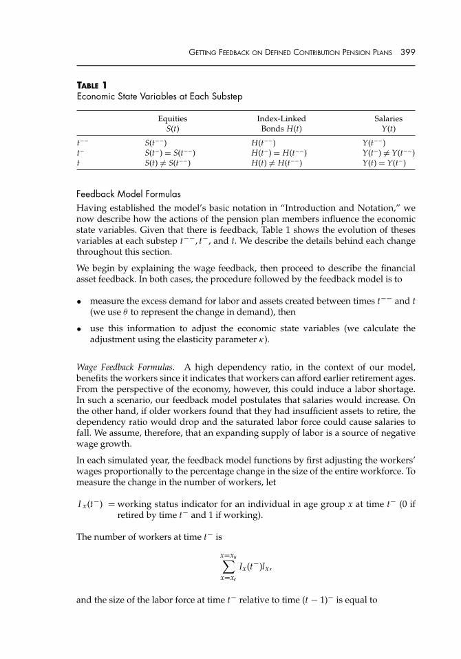
TABLE 1Economic State Variables at Each Substep
Equities Index-Linked SalariesS(t) Bonds H(t) Y(t)
t−− S(t−−) H(t−−) Y(t−−)t− S(t−) = S(t−−) H(t−) = H(t−−) Y(t−) �= Y(t−−)t S(t) �= S(t−−) H(t) �= H(t−−) Y(t) = Y(t−)
Feedback Model FormulasHaving established the model’s basic notation in “Introduction and Notation,” wenow describe how the actions of the pension plan members influence the economicstate variables. Given that there is feedback, Table 1 shows the evolution of thesesvariables at each substep t−−, t−, and t. We describe the details behind each changethroughout this section.
We begin by explaining the wage feedback, then proceed to describe the financialasset feedback. In both cases, the procedure followed by the feedback model is to
• measure the excess demand for labor and assets created between times t−− and t(we use θ to represent the change in demand), then
• use this information to adjust the economic state variables (we calculate theadjustment using the elasticity parameter κ).
Wage Feedback Formulas. A high dependency ratio, in the context of our model,benefits the workers since it indicates that workers can afford earlier retirement ages.From the perspective of the economy, however, this could induce a labor shortage.In such a scenario, our feedback model postulates that salaries would increase. Onthe other hand, if older workers found that they had insufficient assets to retire, thedependency ratio would drop and the saturated labor force could cause salaries tofall. We assume, therefore, that an expanding supply of labor is a source of negativewage growth.
In each simulated year, the feedback model functions by first adjusting the workers’wages proportionally to the percentage change in the size of the entire workforce. Tomeasure the change in the number of workers, let
I x(t−) = working status indicator for an individual in age group x at time t− (0 ifretired by time t− and 1 if working).
The number of workers at time t− is
x=xu∑x=xe
Ix(t−)lx ,
and the size of the labor force at time t− relative to time (t − 1)− is equal to
400 THE JOURNAL OF RISK AND INSURANCE
θY =
x=xu∑x=xe
Ix(t−)lx
x=xu∑x=xe
Ix((t − 1)−)lx
. (12)
In Equation (12), the numerator includes new entrants and takes account of retire-ments between times t−− and t−.
If we assume that, between times t−− and t−, the incremental percentage change inwages is proportional to the incremental percentage change in labor supply, then wecan define κY(<0) as the elasticity of wages with respect to labor supply and:
κY ln θY = lnYx(t−)
Yx(t−−).
Adding this to Equation (6), the feedback model revises the salary for each workingparticipant in age group x between times t−− and t− according to the next formula:
Yx(t−) = Yx(t−−)θκYY
= Yx−1 (t − 1)m(x − xe )
m(x − xe − 1)CPI(t−−)
CPI ((t − 1)−)ex5(t−−)−x5((t−1)−)θκY
Y
= Yx−1 (t − 1)m(x − xe )
m(x − xe − 1)CPI(t−)
CPI ((t − 1)−)ex5(t−)−x5((t−1)−), (13)
where CPI(t−) = CPI(t−−) and x5(t−) − x5(t−−) = κY ln θ Y.
Wealth and Asset Price Feedback Formulas. The process of calculating the feedbackadjustment for equity and index-linked bond prices is similar to the feedback modelfor wages, but somewhat more complicated. According to the widespread theoreticaleffect given in “Previous Literature on the Aggregate Impact of Asset Demand onFinancial Markets,” a greater demand for either asset would increase the value of anyportfolio holding it and vice versa. The feedback model adjusts the prices of equitiesand bonds based on their respective change in demand. Our task is to first determinethe change in asset demand. Let
WSx (t) = total invested in equities by an individual in age group x at time t and
WHx (t) = total invested in index-linked bonds by an individual in age group x at
time t.
Referring back to Equation (11), the equity and index-linked bond wealth for anindividual in age group x at time t−−, based on the provisional returns from timest − 1 to t, are
WSx (t−−) = αWx−1(t − 1)
S(t−−)S(t − 1)
1
1px−1(14)

GETTING FEEDBACK ON DEFINED CONTRIBUTION PENSION PLANS 401
and
WHx (t−−) = (1 − α) Wx−1(t − 1)
H(t−−)H(t − 1)
1
1px−1. (15)
To determine the change in asset demand, we must measure the cash flows into andout of the equity and bond pension accounts. The cash flows are
• the payment of pension benefits for retired members (I x(t−) = 0, which includesthe new retirees at time t−);
• the investment of contributions by working members (I x(t−) = 1);
• in the case of the second inheritance decision scenario, the receipt of inheritance forage groups 20 to 55, and the associated asset liquidation and increase to pensionaccounts;
• the rebalancing of assets to maintain a static investment strategy; and
• in the case of a shift to the less risky asset at retirement in the second invest-ment scenario, the reallocation of funds among assets according to a changinginvestment strategy.
Note that the upcoming formulae reflect the static investment strategy scenario whereall bequests are distributed among surviving members of the deceased’s age group;the formulae do not, therefore contain the third and fifth cash flows. We will presentthe other scenarios and their formulae at the end of this section.
The cash flows occur between times t− and t and they are based on the newly adjustedasset prices. This creates a circular dependence between the actual change in demandand the level of feedback since they are both calculated from the other. Owing tothis circular dependance, we measure each asset’s provisional change in demand tocalculate the feedback. We do so by basing the cash flows that should occur betweentimes t− and t on
• the provisional asset values that have not yet been adjusted by the change indemand (S(t−) and H(t−)) and
• the provisional annuitization interest rate (x3(t−)).
We determine the asset supply at time t−− using Equations (14) and (15). The provi-sional wealth at time t− for a member of age group x is:
Wx(t−) = Wx−1(t − 1)[α
S(t−)S(t − 1)
+ (1 − α)H(t−)
H(t − 1)
]1
1px−1
×[
1 − (1 − Ix(t−))
a x3(t−)x (t)
]+ πYx(t−)Ix(t−). (16)
402 THE JOURNAL OF RISK AND INSURANCE
In Equation (16), the provisional pension wealth for each DC participant accumu-lates forward between times t − 1 and t− with the return on their investment(αS(t−)/S(t − 1) + (1 − α) H(t−)/H(t − 1)), by the bequests of the deceased (1/1px−1)and any provisional cash flows. That is, if the member is employed (I x(t−) = 1), thentheir provisional wealth also increases with a contribution of πYx(t−). Otherwise, fora member who is retired (1 − I x(t−) = 1), their provisional pension income payment
reduces their accumulated provisional pension wealth by a rate of 1/a x3(t−)x (t).
The provisional wealth invested in equities and bonds by an individual in age groupx at time t− is then
WSx (t−) = αWx(t−) (17)
and
WHx (t−) = (1 − α) Wx(t−), (18)
respectively. It follows that, across the population of 81 age groups, we can define theprovisional demand for equities at time t− as a proportion of its supply at time t−−as:
θS =
x=xu∑x=xe
WSx (t−)lx
x=xu∑x=xe
WSx (t−−)lx
. (19)
Similarly, the ratio of the provisional demand for index-linked bonds at time t− as aproportion of its supply at time t−− is:
θH =
x=xu∑x=xe
WHx (t−)lx
x=xu∑x=xe
WHx (t−−)lx
. (20)
If we let κS(>0) represent the elasticity of the equity price with respect to its demand,then equity prices change in the following way, given a provisional change in demandratio of θS:
S(t) = S(t−)θκSS
= S(t − 1)ex2(t−)−x2(t−1)θκSS
= S(t − 1)ex2(t)−x2(t−1), (21)
where x2(t) − x2(t−) = κS ln θS.
GETTING FEEDBACK ON DEFINED CONTRIBUTION PENSION PLANS 403
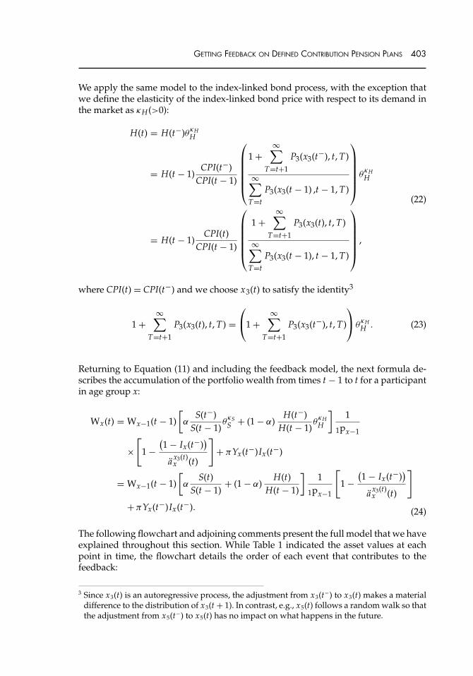
We apply the same model to the index-linked bond process, with the exception thatwe define the elasticity of the index-linked bond price with respect to its demand inthe market as κH(>0):
H(t) = H(t−)θκHH
= H(t − 1)CPI(t−)
CPI(t − 1)
⎛⎜⎜⎜⎜⎜⎝
1 +∞∑
T=t+1
P3(x3(t−), t, T)
∞∑T=t
P3(x3(t − 1) ,t − 1, T)
⎞⎟⎟⎟⎟⎟⎠ θ
κHH
= H(t − 1)CPI(t)
CPI(t − 1)
⎛⎜⎜⎜⎜⎜⎝
1 +∞∑
T=t+1
P3(x3(t), t, T)
∞∑T=t
P3(x3(t − 1), t − 1, T)
⎞⎟⎟⎟⎟⎟⎠ ,
(22)
where CPI(t) = CPI(t−) and we choose x3(t) to satisfy the identity3
1 +∞∑
T=t+1
P3(x3(t), t, T) =⎛⎝1 +
∞∑T=t+1
P3(x3(t−), t, T)
⎞⎠ θ
κHH . (23)
Returning to Equation (11) and including the feedback model, the next formula de-scribes the accumulation of the portfolio wealth from times t − 1 to t for a participantin age group x:
Wx(t) = Wx−1(t − 1)[α
S(t−)S(t − 1)
θκSS + (1 − α)
H(t−)H(t − 1)
θκHH
]1
1px−1
×[
1 −(1 − Ix(t−)
)a x3(t)
x (t)
]+ πYx(t−)Ix(t−)
= Wx−1(t − 1)[α
S(t)S(t − 1)
+ (1 − α)H(t)
H(t − 1)
]1
1px−1
[1 −
(1 − Ix(t−)
)a x3(t)
x (t)
]
+πYx(t−)Ix(t−). (24)
The following flowchart and adjoining comments present the full model that we haveexplained throughout this section. While Table 1 indicated the asset values at eachpoint in time, the flowchart details the order of each event that contributes to thefeedback:
3 Since x3(t) is an autoregressive process, the adjustment from x3(t−) to x3(t) makes a materialdifference to the distribution of x3(t + 1). In contrast, e.g., x5(t) follows a random walk so thatthe adjustment from x5(t−) to x5(t) has no impact on what happens in the future.
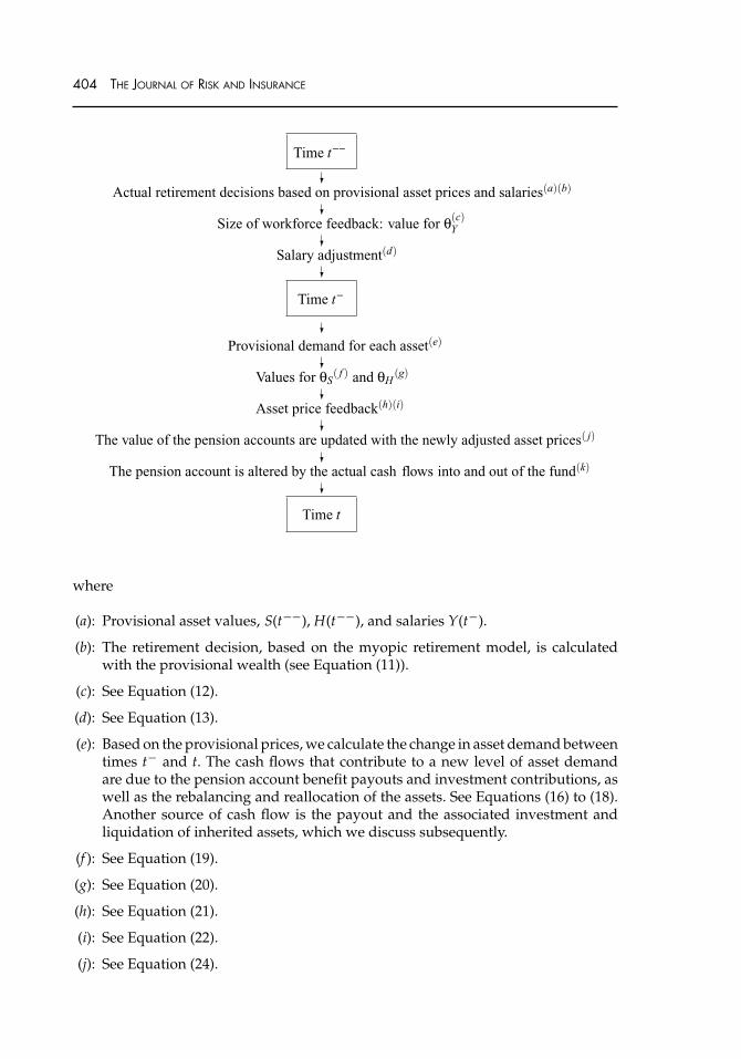
404 THE JOURNAL OF RISK AND INSURANCE
Time t
Actual retirement decisions based on provisional asset prices and salaries(a)(b)
Size of workforce feedback: value for θ(c)Y
Salary adjustment(d)
Time t
Provisional demand for each asset(e)
Values for θS( f ) and θH
(g)
Asset price feedback(h)(i)
The value of the pension accounts are updated with the newly adjusted asset prices( j)
The pension account is altered by the actual cash flows into and out of the fund(k)
Time t
where
(a): Provisional asset values, S(t−−), H(t−−), and salaries Y(t−).
(b): The retirement decision, based on the myopic retirement model, is calculatedwith the provisional wealth (see Equation (11)).
(c): See Equation (12).
(d): See Equation (13).
(e): Based on the provisional prices, we calculate the change in asset demand betweentimes t− and t. The cash flows that contribute to a new level of asset demandare due to the pension account benefit payouts and investment contributions, aswell as the rebalancing and reallocation of the assets. See Equations (16) to (18).Another source of cash flow is the payout and the associated investment andliquidation of inherited assets, which we discuss subsequently.
(f ): See Equation (19).
(g): See Equation (20).
(h): See Equation (21).
(i): See Equation (22).
(j): See Equation (24).
GETTING FEEDBACK ON DEFINED CONTRIBUTION PENSION PLANS 405
(k): The pension fund contributions and benefit payouts are based on the adjustedasset prices (see Equation (24)).
We will now comment on the formula modifications required for other scenarios.First, the use of a fixed α in the preceding formulas implies that the investmentstrategy is static. If the investment strategy changes at retirement, then the α notationwould be replaced by αIx(t−1) in Equations (14) to (18) and (24) so that α1 is the riskyasset allocation before retirement and α0 is the allocation after retirement.
Second, had we wished to change the inheritance decision model so that the bequestswere left only to survivors between ages 20 and 55 years, then Equation (16) wouldchange to
Wx(t−) =⎛⎝Wx−1(t − 1) + 0.1 ×
{x=xu∑x=xe
Wx(t − 1)lx 1qx
}/x=55∑x=20
lx
⎞⎠
×[α
S(t−)S(t − 1)
+ (1 − α)H(t−)
H(t − 1)
]
×[
1 −(1 − Ix(t−)
)a x3(t−)
x (t)
]+ πYx(t−)Ix(t−)
if x = 20 to 55, otherwise
Wx(t−) = Wx−1(t − 1)[α
S(t−)S(t − 1)
+ (1 − α)H(t−)
H(t − 1)
]
×[
1 −(1 − Ix(t−)
)a x3(t−)
x (t)
]+ πYx(t−)Ix(t−).
Equation (24) would be altered with the same changes. In addition, 1/1px−1 would beremoved from Equations (14) and (15). Finally, the denominators of Equations (19) and(20) would be altered to include the total bequests before they are distributed—i.e.,before any asset leakage occurs:
θS =
x=xu∑x=xe
WSx (t−)lx
x=xu∑x=xe
(WS
x (t−−)lx + αWx(t − 1)lxS(t−−)S(t − 1) 1qx
)
=
x=xu∑x=xe
WSx (t−)lx
x=xu∑x=xe
WSx (t−−)lx−1

406 THE JOURNAL OF RISK AND INSURANCE
and
θH =
x=xu∑x=xe
WHx (t−)lx
x=xu∑x=xe
(WH
x (t−−)lx + (1 − α) Wx(t − 1)lxH(t−−)H(t − 1) 1qx
)
=
x=xu∑x=xe
WHx (t−)lx
x=xu∑x=xe
WHx (t−−)lx−1
.
Estimates for κ S, κ H , and κY
We experiment with three levels of feedback. In the first and most extreme scenario,we assume that there is a fixed supply of capital in the index-linked bond and equitymarket, and that our population is living in a closed economy where there are neitheroverseas nor government sectors. This implies unit elasticity (κS = κ H = 1). Forexample, if the aggregate funds directed towards equity doubles (θ S = 2), so toowould the price
S(t)S(t−)
= θκSS
= 2,
so that the total number of units of equity does not change.
Similarly, in our extreme scenario, we let κY = −1 so that there is a fixed level ofproduction and revenue.4 If the labor force suddenly doubled (θ Y = 2), then thewages would need to be halved to accommodate the increased supply of workerswith jobs:
Yx(t−)Yx(t−−)
= θκYY
= 2−1
= 0.5
The likelihood of unit elasticity in the financial market was disputed in “PreviousLiterature on the Aggregate Impact of Asset Demand on Financial Markets.” It is alsoreasonable to suppose that elasticity exists in the level of productivity and revenue.
4 Production is not part of our model, but lower production per worker is implied by lowerwages.

GETTING FEEDBACK ON DEFINED CONTRIBUTION PENSION PLANS 407
If the size of the workforce increases, output and revenue are also likely to increase,suggesting that unit elasticity of wages with respect to labor supply is an excessiveassumption.
We work away from this extreme scenario and first assume that κ S = κH = −κY = 0.5,then = 0.25. If the demand for equity, index-linked bonds, and employment doubledin the 0.5 feedback scenario, then the price of equity and index-linked bonds wouldincrease by 41 percent while wages would decrease in value by 29 percent. At 0.25,the price of equity and index-linked bonds would increase by 19 percent and wageswould decrease by 16 percent. We refer to these three scenarios as low, medium, andhigh feedback, although they could possibly all be considered high in reality. We willalso consider the scenario of no feedback for the purpose of comparison.
SIMULATED RESULTS WITH FEEDBACK
This section presents the simulated results. Our analysis includes four levels of feed-back that we specified in “Estimates for κS, κH , and κY.” Following from our discus-sion in “Previous Literature on the Aggregate Impact of Asset Demand on FinancialMarkets,” we also consider a static and nonstatic investment strategy. Finally, we in-vestigate two inheritance decision models as discussed in “Withdrawals From Death.”In total, we simulate 12 scenarios—four levels of feedback for each of the followingthree populations (A, B, and C):
Population A: the population homogeneously holds a nonstatic investment strategyand inheritance arising from the deceased is redistributed to the survivors withintheir respective cohorts.
Population B: the population homogeneously holds a static investment strategythroughout their lifetimes and inheritance arising from the deceased is redis-tributed to the survivors within their respective cohorts.
Population C: the population homogeneously holds a nonstatic investment strategyand inheritance is distributed evenly across members in cohorts aged 20 to55 years.
Beginning in “Preliminary Results,” the initial outcome of the simulation indicate thatthe feedback model creates lower wage returns and consequently applies an upwardpressure on the mean dependency ratio. For fairer comparison between the feedbackand original model results, we will make an adjustment to the asset-accumulationmodel parameters to realign the rates with their original average. In “Results forPopulation A,” we will analyze the population dependency ratio results at the fourlevels of feedback for Population A. “Dependency Ratio Dynamics for PopulationA” examines this population’s retirement dynamics over time. “Dependency RatioDynamics for Population B” presents the same four scenarios, but for Population B.Finally, “Dependency Ratio Dynamics for Population C” tests the second inheritancedecision model in Population C.
These upcoming sections reveal that incorporating feedback has a smoothing effecton the dependency ratio volatility. The best results occur when the supply of capital
408 THE JOURNAL OF RISK AND INSURANCE
and production is fixed (θ S = θ H = θ Y = 1). Despite the substantial improvement,however, there still remains instability in the dependency ratio.
Preliminary ResultsThis section contains the feedback model’s initial effects on the results. We explainhow the feedback alters the economic processes in the asset-accumulation model sothat they no longer match their historical averages. We consequentially recalibratethe original model to compensate for this side effect.
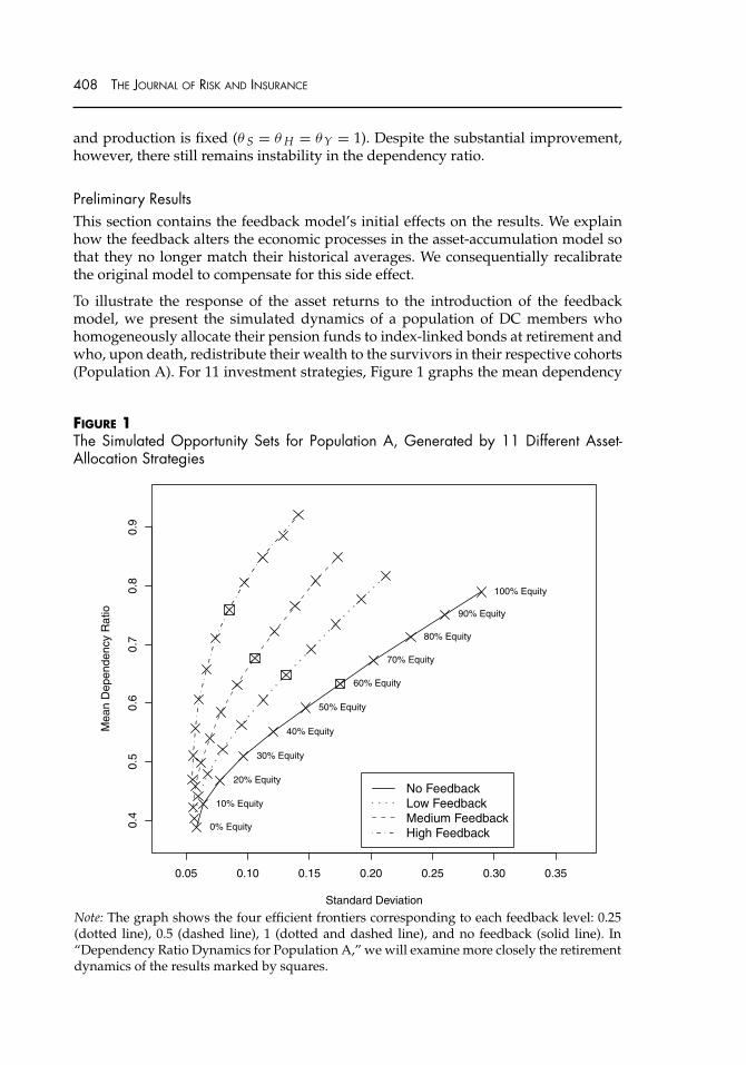
To illustrate the response of the asset returns to the introduction of the feedbackmodel, we present the simulated dynamics of a population of DC members whohomogeneously allocate their pension funds to index-linked bonds at retirement andwho, upon death, redistribute their wealth to the survivors in their respective cohorts(Population A). For 11 investment strategies, Figure 1 graphs the mean dependency
FIGURE 1The Simulated Opportunity Sets for Population A, Generated by 11 Different Asset-Allocation Strategies
0.05 0.10 0.15 0.20 0.25 0.30 0.35
0.4
0.5
0.6
0.7
0.8
0.9
Standard Deviation
Mean D
ependency R
atio
No FeedbackLow FeedbackMedium FeedbackHigh Feedback
0% Equity
10% Equity
20% Equity
30% Equity
40% Equity
50% Equity
60% Equity
70% Equity
80% Equity
90% Equity
100% Equity
Note: The graph shows the four efficient frontiers corresponding to each feedback level: 0.25(dotted line), 0.5 (dashed line), 1 (dotted and dashed line), and no feedback (solid line). In“Dependency Ratio Dynamics for Population A,” we will examine more closely the retirementdynamics of the results marked by squares.
GETTING FEEDBACK ON DEFINED CONTRIBUTION PENSION PLANS 409
ratio over a 4,500 year simulation against its standard deviation. We choose a longerrun as opposed to several shorter ones so that the results are less influenced byinitial conditions. The best outcomes are those with a high mean dependency ratiowith low volatility, indicating early retirement ages among happy citizens while stillmaintaining a stable labor force participation in the population. We plot the efficientfrontier for each feedback scenario, creating four efficient frontiers in total: one foreach of the three levels of feedback and another for the model without the inclusionof feedback. To avoid clutter, only the scenario without feedback has its 11 portfolios,indicated by an “X” marked by its equity content (and the remaining portion of eachportfolio is invested in index-linked bonds).
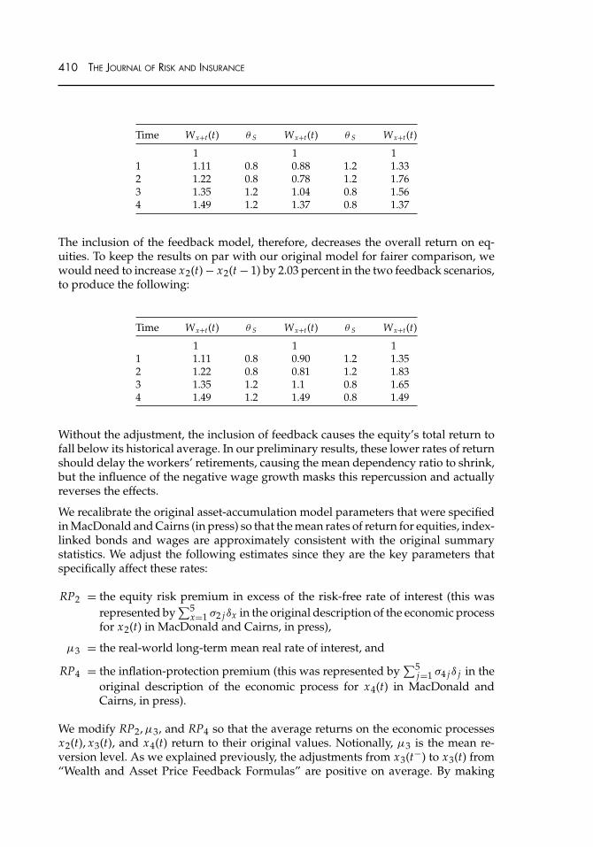
Our first observation is that feedback drives up the mean dependency ratio for allinvestment strategies. This occurs as a result of the the annual recalculation of theinstantaneous risk-free real rate of return (x3(t)), as previously discussed in a footnote.The adjustments from x3(t−) to x3(t) are positive on average. The altered dynamicsof x3(t) affects x4(t) (the CPI process), generating slower wage growth since wagesare primarily moved by inflation in our economic model. In fact, in the high feedbackscenario, the average wage growth drops from over 3 percent to nearly −6 percentwhen funds are initially only invested in equities and to −5.25 percent when they areinitially only invested in index-linked bonds. In our stochastic model, reduced salarygrowth gives rise to earlier retirement ages and, consequently, higher dependencyratios. This reaction is on account of the enhanced appeal of the retirement pensionrelative to the slowly growing salary.5
There are several forces affecting the index-linked bond return—it is both dampenedby the lower inflation as well as boosted by the overall higher real rate of return (x3(t)).Another influence is the feedback itself, which dampens the returns on index-linkedbonds and equities. For example, consider a pension account completely investedin equities where κ S = 1, x2(t) − x2(t − 1) = 0.10 for 4 years, and there are neithercontributions nor pension payments. Without the feedback feature, the original modelwould produce the following progression of wealth, Wx(t), for a participant in agegroup x at t = 0:
Time Wx+t(t)
0 11 1.112 1.223 1.354 1.49
If we include the feedback feature and assume a 20 percent decline in equity demandfor 2 years, followed by 2 years of 20 percent increases (and vice versa), the wealthaccumulation is modified as the next table demonstrates:
5 See Section 4.7 in MacDonald (2007) for a more complete explanation.
410 THE JOURNAL OF RISK AND INSURANCE
Time Wx+t(t) θ S Wx+t(t) θ S Wx+t(t)
1 1 11 1.11 0.8 0.88 1.2 1.332 1.22 0.8 0.78 1.2 1.763 1.35 1.2 1.04 0.8 1.564 1.49 1.2 1.37 0.8 1.37
The inclusion of the feedback model, therefore, decreases the overall return on eq-uities. To keep the results on par with our original model for fairer comparison, wewould need to increase x2(t) − x2(t − 1) by 2.03 percent in the two feedback scenarios,to produce the following:
Time Wx+t(t) θ S Wx+t(t) θ S Wx+t(t)
1 1 11 1.11 0.8 0.90 1.2 1.352 1.22 0.8 0.81 1.2 1.833 1.35 1.2 1.1 0.8 1.654 1.49 1.2 1.49 0.8 1.49
Without the adjustment, the inclusion of feedback causes the equity’s total return tofall below its historical average. In our preliminary results, these lower rates of returnshould delay the workers’ retirements, causing the mean dependency ratio to shrink,but the influence of the negative wage growth masks this repercussion and actuallyreverses the effects.
We recalibrate the original asset-accumulation model parameters that were specifiedin MacDonald and Cairns (in press) so that the mean rates of return for equities, index-linked bonds and wages are approximately consistent with the original summarystatistics. We adjust the following estimates since they are the key parameters thatspecifically affect these rates:
RP2 = the equity risk premium in excess of the risk-free rate of interest (this wasrepresented by
∑5x=1 σ2 jδx in the original description of the economic process
for x2(t) in MacDonald and Cairns, in press),
μ3 = the real-world long-term mean real rate of interest, and
RP4 = the inflation-protection premium (this was represented by∑5
j=1 σ4 jδ j in theoriginal description of the economic process for x4(t) in MacDonald andCairns, in press).
We modify RP2, μ3, and RP4 so that the average returns on the economic processesx2(t), x3(t), and x4(t) return to their original values. Notionally, μ3 is the mean re-version level. As we explained previously, the adjustments from x3(t−) to x3(t) from“Wealth and Asset Price Feedback Formulas” are positive on average. By making
GETTING FEEDBACK ON DEFINED CONTRIBUTION PENSION PLANS 411
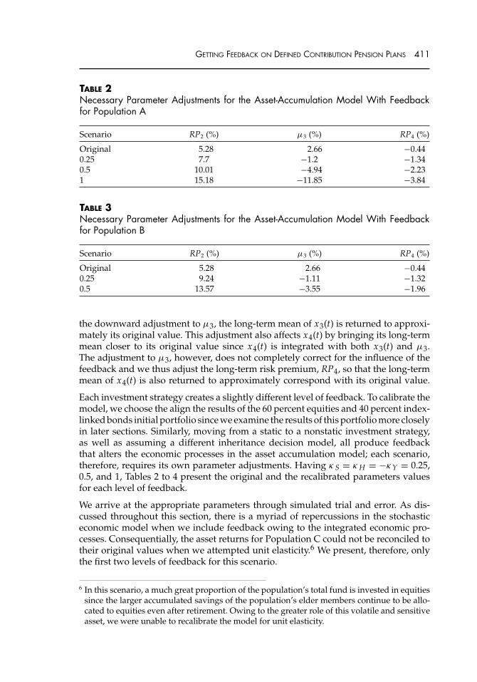
TABLE 2Necessary Parameter Adjustments for the Asset-Accumulation Model With Feedbackfor Population A
Scenario RP2 (%) μ3 (%) RP4 (%)
Original 5.28 2.66 −0.440.25 7.7 −1.2 −1.340.5 10.01 −4.94 −2.231 15.18 −11.85 −3.84
TABLE 3Necessary Parameter Adjustments for the Asset-Accumulation Model With Feedbackfor Population B
Scenario RP2 (%) μ3 (%) RP4 (%)
Original 5.28 2.66 −0.440.25 9.24 −1.11 −1.320.5 13.57 −3.55 −1.96
the downward adjustment to μ3, the long-term mean of x3(t) is returned to approxi-mately its original value. This adjustment also affects x4(t) by bringing its long-termmean closer to its original value since x4(t) is integrated with both x3(t) and μ3.The adjustment to μ3, however, does not completely correct for the influence of thefeedback and we thus adjust the long-term risk premium, RP4, so that the long-termmean of x4(t) is also returned to approximately correspond with its original value.
Each investment strategy creates a slightly different level of feedback. To calibrate themodel, we choose the align the results of the 60 percent equities and 40 percent index-linked bonds initial portfolio since we examine the results of this portfolio more closelyin later sections. Similarly, moving from a static to a nonstatic investment strategy,as well as assuming a different inheritance decision model, all produce feedbackthat alters the economic processes in the asset accumulation model; each scenario,therefore, requires its own parameter adjustments. Having κ S = κ H = −κY = 0.25,0.5, and 1, Tables 2 to 4 present the original and the recalibrated parameters valuesfor each level of feedback.
We arrive at the appropriate parameters through simulated trial and error. As dis-cussed throughout this section, there is a myriad of repercussions in the stochasticeconomic model when we include feedback owing to the integrated economic pro-cesses. Consequentially, the asset returns for Population C could not be reconciled totheir original values when we attempted unit elasticity.6 We present, therefore, onlythe first two levels of feedback for this scenario.
6 In this scenario, a much great proportion of the population’s total fund is invested in equitiessince the larger accumulated savings of the population’s elder members continue to be allo-cated to equities even after retirement. Owing to the greater role of this volatile and sensitiveasset, we were unable to recalibrate the model for unit elasticity.
412 THE JOURNAL OF RISK AND INSURANCE
TABLE 4Necessary Parameter Adjustments for the Asset-Accumulation Model With Feedbackfor Population C
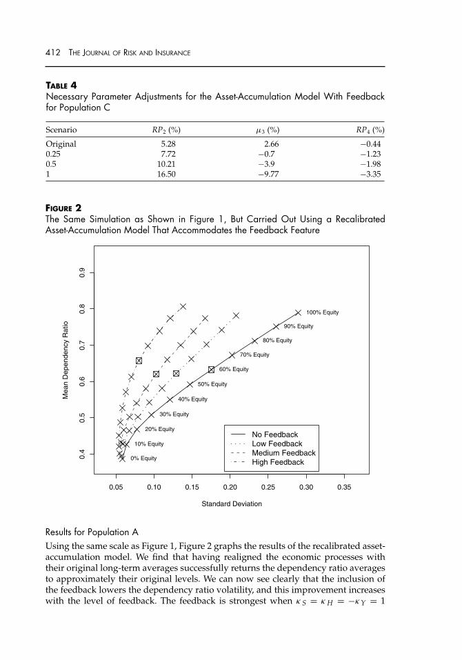
Scenario RP2 (%) μ3 (%) RP4 (%)
Original 5.28 2.66 −0.440.25 7.72 −0.7 −1.230.5 10.21 −3.9 −1.981 16.50 −9.77 −3.35
FIGURE 2The Same Simulation as Shown in Figure 1, But Carried Out Using a RecalibratedAsset-Accumulation Model That Accommodates the Feedback Feature
0.05 0.10 0.15 0.20 0.25 0.30 0.35
0.4
0.5
0.6
0.7
0.8
0.9
Standard Deviation
Mean D
ependency R
atio
No FeedbackLow FeedbackMedium FeedbackHigh Feedback
0% Equity
10% Equity
20% Equity
30% Equity
40% Equity
50% Equity
60% Equity
70% Equity
80% Equity
90% Equity
100% Equity
Results for Population AUsing the same scale as Figure 1, Figure 2 graphs the results of the recalibrated asset-accumulation model. We find that having realigned the economic processes withtheir original long-term averages successfully returns the dependency ratio averagesto approximately their original levels. We can now see clearly that the inclusion ofthe feedback lowers the dependency ratio volatility, and this improvement increaseswith the level of feedback. The feedback is strongest when κ S = κ H = −κY = 1
GETTING FEEDBACK ON DEFINED CONTRIBUTION PENSION PLANS 413
and the investment strategy is 100 percent equities. The volatility in the dependencyratio is impressively halved in this extreme scenario, reducing it from approximately29 percent to 14 percent. The 14 percent standard deviation, however, could potentiallynot be low enough.
It is possible that a by-product of the feedback model is a reduction in the equityreturn risk, thus explaining the decline in the dependency ratio volatility. This is,however, not the cause since the volatility of the log equity returns actually lowersonly slightly after the inclusion of feedback when the feedback is strongest. Thenoteworthy reduction in the dependency ratio fluctuations is indeed attributable tothe feedback.
Dependency Ratio Dynamics for Population AIn this section, we wish to get a fuller picture of the impact of the feedback model andthe remaining dependency ratio fluctuation. This section ascertains that, although thefeedback mitigates the extreme results that were originally produced, the dependencyratio still remains unstable.
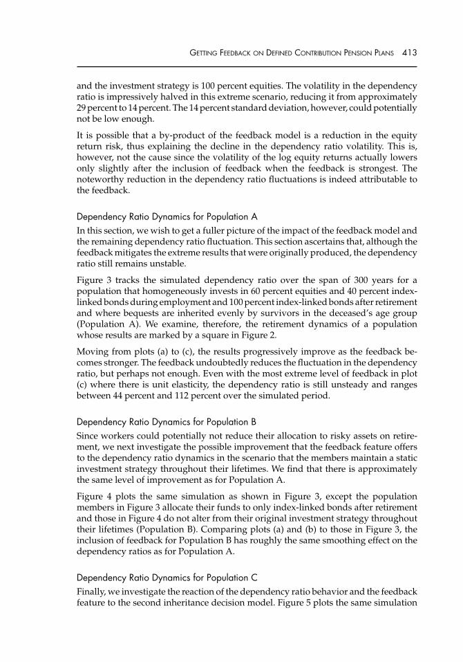
Figure 3 tracks the simulated dependency ratio over the span of 300 years for apopulation that homogeneously invests in 60 percent equities and 40 percent index-linked bonds during employment and 100 percent index-linked bonds after retirementand where bequests are inherited evenly by survivors in the deceased’s age group(Population A). We examine, therefore, the retirement dynamics of a populationwhose results are marked by a square in Figure 2.
Moving from plots (a) to (c), the results progressively improve as the feedback be-comes stronger. The feedback undoubtedly reduces the fluctuation in the dependencyratio, but perhaps not enough. Even with the most extreme level of feedback in plot(c) where there is unit elasticity, the dependency ratio is still unsteady and rangesbetween 44 percent and 112 percent over the simulated period.
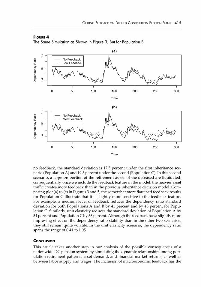
Dependency Ratio Dynamics for Population BSince workers could potentially not reduce their allocation to risky assets on retire-ment, we next investigate the possible improvement that the feedback feature offersto the dependency ratio dynamics in the scenario that the members maintain a staticinvestment strategy throughout their lifetimes. We find that there is approximatelythe same level of improvement as for Population A.
Figure 4 plots the same simulation as shown in Figure 3, except the populationmembers in Figure 3 allocate their funds to only index-linked bonds after retirementand those in Figure 4 do not alter from their original investment strategy throughouttheir lifetimes (Population B). Comparing plots (a) and (b) to those in Figure 3, theinclusion of feedback for Population B has roughly the same smoothing effect on thedependency ratios as for Population A.
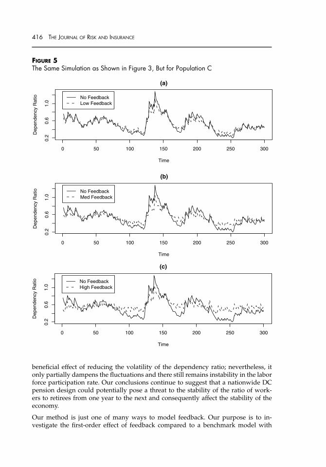
Dependency Ratio Dynamics for Population CFinally, we investigate the reaction of the dependency ratio behavior and the feedbackfeature to the second inheritance decision model. Figure 5 plots the same simulation
414 THE JOURNAL OF RISK AND INSURANCE
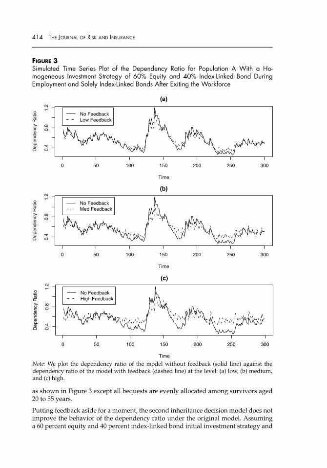
FIGURE 3Simulated Time Series Plot of the Dependency Ratio for Population A With a Ho-mogeneous Investment Strategy of 60% Equity and 40% Index-Linked Bond DuringEmployment and Solely Index-Linked Bonds After Exiting the Workforce
0 50 100 150 200 250 300
0.4
0.8
1.2
(a)
Time
De
pe
nd
en
cy R
atio No Feedback
Low Feedback
0 50 100 150 200 250 300
0.4
0.8
1.2
(b)
Time
De
pe
nd
en
cy R
atio No Feedback
Med Feedback
0 50 100 150 200 250 300
0.4
0.8
1.2
(c)
Time
De
pe
nd
en
cy R
atio No Feedback
High Feedback
Note: We plot the dependency ratio of the model without feedback (solid line) against thedependency ratio of the model with feedback (dashed line) at the level: (a) low, (b) medium,and (c) high.
as shown in Figure 3 except all bequests are evenly allocated among survivors aged20 to 55 years.
Putting feedback aside for a moment, the second inheritance decision model does notimprove the behavior of the dependency ratio under the original model. Assuminga 60 percent equity and 40 percent index-linked bond initial investment strategy and
GETTING FEEDBACK ON DEFINED CONTRIBUTION PENSION PLANS 415
FIGURE 4The Same Simulation as Shown in Figure 3, But for Population B
0 50 100 150 200 250 300
0.4
0.8
1.2
(a)
Time
Dependency R
atio No Feedback
Low Feedback
0 50 100 150 200 250 300
0.4
0.8
1.2
(b)
Time
Dependency R
atio No Feedback
Med Feedback
no feedback, the standard deviation is 17.5 percent under the first inheritance sce-nario (Population A) and 19.3 percent under the second (Population C). In this secondscenario, a large proportion of the retirement assets of the deceased are liquidated;consequentially, once we include the feedback feature in the model, the heavier assettraffic creates more feedback than in the previous inheritance decision model. Com-paring plot (a) to (c) in Figures 3 and 5, the somewhat more flattened feedback resultsfor Population C illustrate that it is slightly more sensitive to the feedback feature.For example, a medium level of feedback reduces the dependency ratio standarddeviation for both Populations A and B by 41 percent and by 43 percent for Popu-lation C. Similarly, unit elasticity reduces the standard deviation of Population A by54 percent and Population C by 56 percent. Although the feedback has a slightly moreimproving effect on the dependency ratio stability than in the other two scenarios,they still remain quite volatile. In the unit elasticity scenario, the dependency ratiospans the range of 0.41 to 1.05.
CONCLUSION
This article takes another step in our analysis of the possible consequences of anationwide DC pension system by simulating the dynamic relationship among pop-ulation retirement patterns, asset demand, and financial market returns, as well asbetween labor supply and wages. The inclusion of macroeconomic feedback has the
416 THE JOURNAL OF RISK AND INSURANCE
FIGURE 5The Same Simulation as Shown in Figure 3, But for Population C
0 50 100 150 200 250 300
0.2
0.6
1.0
(a)
Time
De
pe
nd
en
cy R
atio No Feedback
Low Feedback
0 50 100 150 200 250 300
0.2
0.6
1.0
(b)
Time
De
pe
nd
en
cy R
atio No Feedback
Med Feedback
0 50 100 150 200 250 300
0.2
0.6
1.0
(c)
Time
De
pe
nd
en
cy R
atio No Feedback
High Feedback
beneficial effect of reducing the volatility of the dependency ratio; nevertheless, itonly partially dampens the fluctuations and there still remains instability in the laborforce participation rate. Our conclusions continue to suggest that a nationwide DCpension design could potentially pose a threat to the stability of the ratio of work-ers to retirees from one year to the next and consequently affect the stability of theeconomy.
Our method is just one of many ways to model feedback. Our purpose is to in-vestigate the first-order effect of feedback compared to a benchmark model with
GETTING FEEDBACK ON DEFINED CONTRIBUTION PENSION PLANS 417
no feedback. Alternative formulations might, for example, allow potential retireesto review their retirement decisions once asset prices have been adjusted for feed-back. Future work could improve on our DC population modeling by tying togetherconsumption, production, and income. In addition, since our feedback model is acrude first approximation to find market equilibrium, future work could incorpo-rate a feedback model that finds the market equilibrium—where the asset prices areadjusted until the supply is equal to the demand.
REFERENCES
Ang, A., and A. Maddaloni, 2003, Do Demographic Changes Affect Risk Premiums?Evidence From International Data, NBER Working Paper No. 9677.
Arias, E., 2004, United States Life Tables, 2002, National Vital Statistics Reports, 53(6):1-39.
Blake, D., A. J. G. Cairns, and K. Dowd, 2003, PensionMetrics 2: Stochastic PensionPlan Design During the Distribution Phase, Insurance: Mathematics and Economics,33: 29-47.
Bosworth, B. P., R. C. Bryant, and G. Burtless, 2004, The Impact of Aging on FinancialMarkets and the Economy: A Survey, Working Paper, The Brookings Institution.
Brooks, R. J., 2002, Asset Market Effects of the Baby-Boom and Social Security Reform,American Economic Review, 92: 402-406.
Brown, J. R., and M. J. Warshawsky, 2001, Longevity-Insured Retirement Distributionsfrom Pension Plans: Market and Regulatory Issues, NBER Working Paper No. 8064.
Davidoff, T., J. R. Brown, and P. A. Diamond, 2005, Annuities and Individual Welfare,American Economic Review, 95(5): 1573-1590.
Lachance, M.-E., 2003, Optimal Investment Behavior as Retirement Looms, WorkingPaper, Wharton School, University of Pennsylvania.
MacDonald, B.-J., 2007, The Impact of Defined Contribution Pension Plans on Popu-lation Retirement Dynamics, PhD thesis, Heriot-Watt University, Edinburgh, UK.
MacDonald, B.-J., and A. J. G. Cairns, in press, The Impact of DC Pension Systems onPopulation Dynamics. North American Actuarial Journal.
McGill, D. M., K. N. Brown, J. J. Haley, and S. J. Schieber, 1996, Fundamentals of PrivatePensions, 7th edition (Philadelphia, PA: University of Pennsylvania Press).
Organisation for Economic Co-Operation and Development, 2005, Ageing and PensionSystem Reform: Implications for Financial Markets and Economic Policies (Paris: OECD).
Poterba, J. M., 2004, The Impact of Population Ageing on Financial Markets, NBERWorking Paper No. 10851.
Poterba, J. M., S. F. Venti, and D. A. Wise, 2005, Demographic Change, RetirementSaving, and Financial Market Returns: Part 1, National Bureau of Economic ResearchPapers on Retirement Research Center Projects NB05-01 (Cambridge, MA: NBER).
Stock, J. H., and D. A. Wise, 1990, Pensions, the Option Value of Work, and Retirement,Econometrica, 58(5): 1151-1180.
Vasicek, O. E., 1977, An Equilibrium Characterisation of the Term Structure, Journalof Financial Economics, 5(2): 177-188.