Geophysical Journal International - ISTerre · 1G´eoazur, Universit e Nice-Sophia Antipolis, CNRS, IRD, ... Mora 1987, 1988; Neves & Singh 1996), the beneﬁts of wide apertures

Geophys. J. Int. (2011) 187, 1495–1515 doi: 10.1111/j.1365-246X.2011.05209.x

GJI

Sei

smol

ogy

On the footprint of anisotropy on isotropic full waveform inversion:the Valhall case study

Vincent Prieux,1 Romain Brossier,2 Yaser Gholami,1 Stephane Operto,3 Jean Virieux,2

O. I. Barkved4 and J. H. Kommedal41Geoazur, Universite Nice-Sophia Antipolis, CNRS, IRD, Observatoire de la Cote d’Azur, Valbonne, France.2ISTerre, Observatoire des Sciences de l’Univers de Grenoble, Universite Joseph Fourier, BP 53, 38041 Grenoble, Cedex 9, France.3Geoazur, Universite Nice-Sophia Antipolis, CNRS, IRD, Observatoire de la Cote d’Azur, Villefranche-sur-mer, France. E-mail: [email protected] Norge, Stavanger, Norway

Accepted 2011 August 26. Received 2011 August 3; in original form 2011 March 28

S U M M A R YThe validity of isotropic approximation to perform acoustic full waveform inversion (FWI) ofreal wide-aperture anisotropic data can be questioned due to the intrinsic kinematic inconsis-tency between short- and large-aperture components of the data. This inconsistency is mainlyrelated to the differences between the vertical and horizontal velocities in vertical-transverseisotropic (VTI) media. The footprint of VTI anisotropy on 2-D acoustic isotropic FWI is illus-trated on a hydrophone data set of an ocean-bottom cable that was collected over the Valhallfield in the North Sea. Multiscale FWI is implemented in the frequency domain by hierar-chical inversions of increasing frequencies and decreasing aperture angles. The FWI modelsare appraised by local comparison with well information, seismic modelling, reverse-timemigration (RTM) and source-wavelet estimation. A smooth initial VTI model parameterizedby the vertical velocity V 0 and the Thomsen parameters δ and ε were previously developedby anisotropic reflection traveltime tomography. The normal moveout (VNMO = V0

√1 + 2δ)

and horizontal (Vh = V0√

1 + 2ε) velocity models were inferred from the anisotropic modelsto perform isotropic FWI. The V NMO models allows for an accurate match of short-spreadreflection traveltimes, whereas the V h model, after updating by first-arrival traveltime tomog-raphy (FATT), allows for an accurate match of first-arrival traveltimes. Ray tracing in thevelocity models shows that the first 1.5 km of the medium are sampled by both diving wavesand reflections, whereas the deeper structure at the reservoir level is mainly controlled byshort-spread reflections. Starting from the initial anisotropic model and keeping fixed δ and ε

models, anisotropic FWI allows us to build a vertical velocity model that matches reasonablywell the well-log velocities. Isotropic FWI is performed using either the NMO model or theFATT model as initial model. In both cases, horizontal velocities are mainly reconstructed inthe first 1.5 km of the medium. This suggests that the wide-aperture components of the datahave a dominant control on the velocity estimation at these depths. These high velocities inthe upper structure lead to low values of velocity in the underlying gas layers (either equal orlower than vertical velocities of the well log), and/or a vertical stretching of the structure at thereservoir level below the gas. This bias in the gas velocities and the mispositioning in depth ofthe deep reflectors, also shown in the RTM images, are required to match the deep reflectionsin the isotropic approximation and highlight the footprint of anisotropy in the isotropic FWI oflong-offset data. Despite the significant differences between the anisotropic and isotropic FWImodels, each of these models produce a nearly-equivalent match of the data, which highlightsthe ill-posedness of acoustic anisotropic FWI. Hence, we conclude with the importance ofconsidering anisotropy in FWI of wide-aperture data to avoid bias in the velocity reconstruc-tions and mispositioning in depth of reflectors. Designing a suitable parameterization of theVTI acoustic FWI is a central issue to manage the ill-posedness of the FWI.

Key words: Inverse theory; Controlled source seismology; Seismic anisotropy; Seismictomography; Computational seismology; Wave propagation.

C© 2011 The Authors 1495Geophysical Journal International C© 2011 RAS

Geophysical Journal International

1496 V. Prieux et al.

I N T RO D U C T I O N

Full waveform inversion (FWI) is a multiscale data-fitting approachfor velocity-model building from wide-aperture/wide-azimuth ac-quisition geometries (Pratt 1999). Since the pioneering works onFWI in the eighties (Gauthier et al. 1986; Mora 1987, 1988; Neves& Singh 1996), the benefits of wide apertures or long offsets toreconstruct long and intermediate wavelengths of a medium, andhence, to improve FWI resolution, have been recognized. In theframework of frequency-domain FWI, Pratt & Worthington (1990);Pratt et al. (1996); Pratt (1999); Sirgue & Pratt (2004) also showhow the redundant wavenumber coverage provided by wide-aperturesurveys can be taken advantage of in the design of efficient FWIalgorithms, as applied to decimated data sets that correspond to afew discrete frequencies. On the other hand, wide apertures andlong offsets increase the non-linearity of the inversion, because thewave fronts integrate the medium complexity over many propa-gated wavelengths, and then make the local optimization subject tocycle-skipping artefacts (Sirgue 2006; Pratt 2008). Cycle skippingartefacts will arise when the relative traveltime error, namely, the ra-tio between the traveltime error and the duration of the simulation,exceeds half of the inverse of the number of propagated wave-lengths (Pratt 2008; Virieux & Operto 2009). The most efficientapproach to mitigate these non-linearities consists of the recordingand inverting of sufficiently low frequencies. For typical hydrocar-bon exploration surveys with a few kilometres penetration depth,maximum recording distances 10–20 km and maximum recordingtimes 10–20 s, these frequencies can be as low as 1.5–2 Hz, andcorrespond to few propagated wavelengths (Plessix 2009; Plessixet al. 2010; Plessix & Perkins 2010). These quite low frequenciescan allow the FWI to be started from a crude laterally-homogeneousinitial model (Plessix et al. 2010). Alternatively, several multiscalestrategies have been proposed to mitigate the non-linearity of theFWI. The most usual one consists of hierarchical inversions of sub-datasets of increasing high-frequency content (Bunks et al. 1995).In the frequency-domain, these sub-datasets generally correspondto a few discrete frequencies, which are inverted sequentially fromthe lower frequencies to the higher frequencies (e.g. Ravaut et al.2004; Sirgue & Pratt 2004; Operto et al. 2006; Jaiswal et al. 2009).A second level of multiscaling can be implemented by hierarchi-cal inversions of decreasing aperture angles through time damping(Brenders & Pratt 2007; Brossier et al. 2009a; Shin & Ha 2009) ordouble beam-forming (Brossier & Roux 2011), or by using offsetwindows in the framework of layer-stripping approaches (Shipp &Singh 2002; Wang & Rao 2009).

Most of the recent applications of FWI to real wide-aperture datahave been performed in isotropic acoustic approximations, whereonly the reconstruction of the P-wave velocity is sought (e.g. Ravautet al. 2004; Operto et al. 2006; Bleibinhaus et al. 2007; Jaiswal et al.2009). In this framework, it is possible to question the real meaningof the reconstructed velocity, and therefore, of the validity of theisotropic approximation for the inversion of wide-aperture data,which potentially contain a significant footprint of anisotropy. Ananalysis of this footprint is presented by Pratt & Sams (1996), whoapply isotropic and anisotropic first-arrival traveltime tomography(FATT) to cross-hole data recorded in a fractured, highly-layeredmedium. They show the need to incorporate anisotropic effects intothe tomography, to reconcile cross-hole seismic velocities with wellinformation. A FWI case study is also presented by Pratt et al.(2001), who show that isotropic and anisotropic FWI of cross-hole data allow them to match the data equally well. However,the anisotropic velocity model is significantly smoother than its

isotropic counterpart, which suggests some layer-induced extrinsicanisotropy in the isotropic reconstruction. More recent case studiesof mono-parameter anisotropic FWI are briefly presented by Plessix& Perkins (2010) and Vigh et al. (2010).

In this study, we have addressed the validity of the isotropic ap-proximation in the framework of FWI of surface wide-aperture datathrough a case study of real data from the Valhall field in the NorthSea. This case study clearly highlights the footprint of vertical-transverse isotropic (VTI) anisotropy on the velocity reconstructionperformed by isotropic FWI of the wide-aperture data.

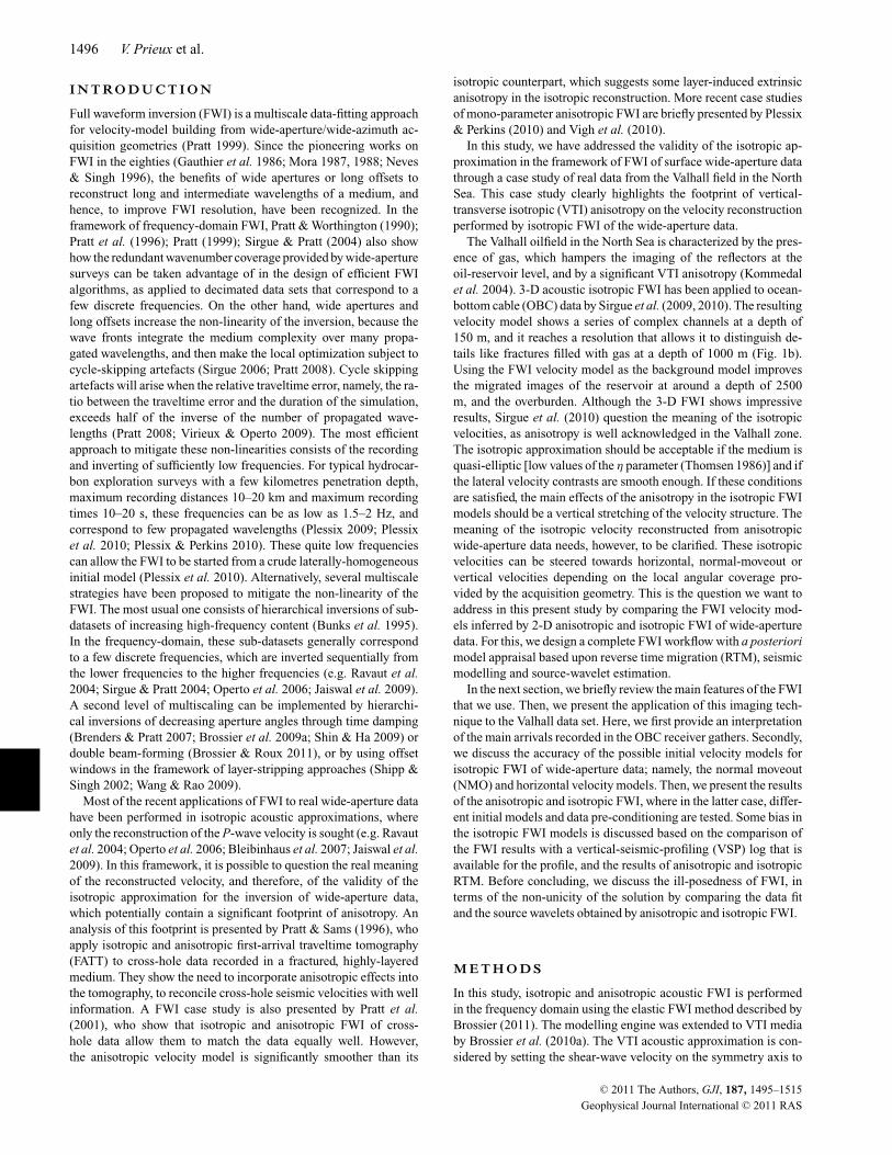
The Valhall oilfield in the North Sea is characterized by the pres-ence of gas, which hampers the imaging of the reflectors at theoil-reservoir level, and by a significant VTI anisotropy (Kommedalet al. 2004). 3-D acoustic isotropic FWI has been applied to ocean-bottom cable (OBC) data by Sirgue et al. (2009, 2010). The resultingvelocity model shows a series of complex channels at a depth of150 m, and it reaches a resolution that allows it to distinguish de-tails like fractures filled with gas at a depth of 1000 m (Fig. 1b).Using the FWI velocity model as the background model improvesthe migrated images of the reservoir at around a depth of 2500m, and the overburden. Although the 3-D FWI shows impressiveresults, Sirgue et al. (2010) question the meaning of the isotropicvelocities, as anisotropy is well acknowledged in the Valhall zone.The isotropic approximation should be acceptable if the medium isquasi-elliptic [low values of the η parameter (Thomsen 1986)] and ifthe lateral velocity contrasts are smooth enough. If these conditionsare satisfied, the main effects of the anisotropy in the isotropic FWImodels should be a vertical stretching of the velocity structure. Themeaning of the isotropic velocity reconstructed from anisotropicwide-aperture data needs, however, to be clarified. These isotropicvelocities can be steered towards horizontal, normal-moveout orvertical velocities depending on the local angular coverage pro-vided by the acquisition geometry. This is the question we want toaddress in this present study by comparing the FWI velocity mod-els inferred by 2-D anisotropic and isotropic FWI of wide-aperturedata. For this, we design a complete FWI workflow with a posteriorimodel appraisal based upon reverse time migration (RTM), seismicmodelling and source-wavelet estimation.

In the next section, we briefly review the main features of the FWIthat we use. Then, we present the application of this imaging tech-nique to the Valhall data set. Here, we first provide an interpretationof the main arrivals recorded in the OBC receiver gathers. Secondly,we discuss the accuracy of the possible initial velocity models forisotropic FWI of wide-aperture data; namely, the normal moveout(NMO) and horizontal velocity models. Then, we present the resultsof the anisotropic and isotropic FWI, where in the latter case, differ-ent initial models and data pre-conditioning are tested. Some bias inthe isotropic FWI models is discussed based on the comparison ofthe FWI results with a vertical-seismic-profiling (VSP) log that isavailable for the profile, and the results of anisotropic and isotropicRTM. Before concluding, we discuss the ill-posedness of FWI, interms of the non-unicity of the solution by comparing the data fitand the source wavelets obtained by anisotropic and isotropic FWI.

M E T H O D S

In this study, isotropic and anisotropic acoustic FWI is performedin the frequency domain using the elastic FWI method described byBrossier (2011). The modelling engine was extended to VTI mediaby Brossier et al. (2010a). The VTI acoustic approximation is con-sidered by setting the shear-wave velocity on the symmetry axis to

C© 2011 The Authors, GJI, 187, 1495–1515

Geophysical Journal International C© 2011 RAS

Effects of anisotropy on full waveform inversion 1497

Figure 1. The Valhall experiment. (a) Layout of the Valhall survey. Points and lines denote the positions of shots and the 4C-OBC, respectively. Cable 21 isthe 2-D line considered in this study. (b) Horizontal slice at a depth of 1000 m across the gas cloud extracted from the 3D-FWI model of Sirgue et al. (2010)(from Sirgue et al. (2009)). The black line matches the position of cable 21. The black circle gives the position of the well log. (c) Vertical-velocity well logextracted at position x = 9500 m (courtesy of BP).

zero and the pressure wavefield is approximated by the average ofthe normal stresses (Brossier et al. 2010a). The seismic modellingis performed in the frequency domain with a velocity-stress dis-continuous Galerkin (DG) method on unstructured triangular mesh,which allows for accurate positioning of the sources and receivers,and accurate parameterization of the bathymetry in the frameworkof the shallow-water environment of Valhall (Brossier et al. 2008;Brossier 2011). In the frequency domain, seismic modelling can berecast in matrix form as

Au = s, (1)

where A is the sparse impedance matrix, which is also known as theforward problem operator. This depends on the frequency, the meshgeometry, the DG interpolation order of each cell and the physicalproperties. The monochromatic wavefield vector is denoted by uand contains the pressure and particle velocity components at eachdegree of freedom of the mesh. The source vector is denoted bys. We solve eq. (1) with the Multifrontal Massively Parallel Sparse(MUMPS) direct solver (MUMPS-team 2009).

The inverse problem is recast as a local optimization where anorm of the data residual vector �d = dobs − dcal(m) in the vicinityof an initial model should be minimized iteratively. The vectors dobs

and dcal(m) denote the observed and modelled data, respectively,

where dcal(m) = S u(m), and the restriction operator S extracts thevalues of the modelled wavefield u at the receiver positions.

In this study, the misfit function is defined by the weighted least-absolute-value (L1) norm of the data residual vector. We choose theL1 norm in the data space because it has been shown to be lesssensitive to noise in the framework of efficient frequency-domainFWI (Brossier et al. 2010b), leading us to the following definitionof the misfit function,

C =∑

i=1,N

|sdi �di |, (2)

where |x| = (xx∗)1/2 and N is the dimension of the data residualvector. In eq. (2), the coefficients sdi of a diagonal weighting operatorWd controls the relative weight of each element of the data residualvector. The updated model at iteration (n + 1) is related to the initialmodel [i.e., the final model of iteration (n)] and to the perturbationmodel δm(n) by

m(n+1) = m(n) + α(n)δm(n), (3)

where α(n) denotes the step length estimated by line search. Min-imization of the misfit function, eq. (2), leads to the followingexpression of the perturbation model δm

δm(n) = −B(n)−1∇C (n), (4)

C© 2011 The Authors, GJI, 187, 1495–1515



where the operator B(n) denotes the Hessian matrix (e.g. Tarantola2005). In this study, we shall use only the diagonal terms of theso-called approximate Hessian matrix (i.e. the linear part of thefull Hessian) damped by a pre-whitening factor (Ravaut et al. 2004,their eq. 15), as a pre-conditioner of the Polak & Ribiere (1969) pre-conditioned conjugate-gradient method, where the diagonal termsof the approximate Hessian are aimed at correcting for geometricalspreading of the data residuals and the partial derivative wavefields.Moreover, the descent direction is steered towards smooth modelsby filtering out the high-wavenumber components of the gradientby 2-D Gaussian smoothing (e.g. Sirgue & Pratt 2004; Ravaut et al.2004; Guitton et al. 2010). The gradient ∇C of the misfit functionC is computed using the adjoint-state method (Plessix 2006), whichgives the following expression for the gradient,

∇Cmi = −�{

ut ∂AT

∂miλ}, (5)

where the real part of a complex number is denoted by �, theconjugate of a complex number by the sign −, and the so-calledadjoint wavefield by λ. In eq. (5), the gradient is given for onefrequency and one source. The gradient that corresponds to multiplesources and frequencies is computed as the sum of the elementarygradients associated with each source–frequency couple. For theL1 norm, the adjoint wavefield is computed by back-propagatingthe weighted data residuals that are normalized by their modulus(Brossier et al. 2010b),

Aλ = S t r, (6)

where r i = sdi �di/|�di |. The operator ∂A/∂mi, eq. (5), describesthe radiation pattern of the virtual secondary source of the partialderivative wavefield with respect to the model parameter mi (Prattet al. 1998).

To increase the quadratic-well-posedness of the inverse problem(Chavent 2009, p. 162), the FWI algorithm is designed into a multi-scale reconstruction of the targeted medium (Brossier et al. 2009a;Brossier 2011). The first level of multiscaling is controlled by theouter loop over the frequency groups, where a frequency groupdefines a subset of simultaneously-inverted frequencies. The multi-scale algorithm proceeds over frequency groups of higher-frequencycontent, with possible overlap between frequency groups. A secondlevel of multiscaling is implemented within a second loop over ex-ponential time-damping applied from the first-arrival times t0. Thetime-damping is implemented in the frequency domain by meansof complex-valued frequencies, where the imaginary part of thefrequency controls the amount of damping (Brenders & Pratt 2007;Brossier et al. 2009a; Shin & Ha 2009). A damped wavefield u canbe written in the frequency domain as

u

(ω + i

τ

)e

t0τ =

∫ +∞

−∞u(t)e− (t−t0)

τ eiωt dt, (7)

where τ is the time-damping factor (s). The time-dampingpre-conditioning injects in progressively more data during onefrequency-group inversion: specifically shorter-aperture seismic ar-rivals are progressively involved as the time-damping factor τ

increases. During the early stages of the frequency-group inver-sion, the early-arriving phases are mainly used to favour the long-wavelength reconstructions in the framework of the multiscaleimaging (Sheng et al. 2006). Frequency-domain FWI algorithmsbased upon the two loops over the real part and the imaginary partsof the frequency domain were also referred to as Fourier–Laplaceinversion by Shin & Ha (2009).

In real-data application, the source-wavelet signature s(ω) is gen-erally unknown, and so it must be estimated for each frequency. Asthe source is linearly related to the wavefield (see eq. 1), the source-wavelet signature can be estimated by solving a least-squares linearinverse problem, assuming that the medium is known. FollowingPratt (1999), we reconstructed the source function s in the frequencydomain through the expression

s(ω) = gcal(ω)Td∗obs(ω)

gcal(ω)Tg∗cal(ω)

, (8)

where gcal denotes the Green functions at the receiver positionsthrough the relationship dcal(ω) = s(ω)gcal(ω). In the frameworkof the adjoint-state method, for consistency with the model updateperformed with an L1 norm minimization, the source signature canalso be estimated alternatively with an L1 norm minimization (R.-E. Plessix, personal communication, 2010). Such optimization hasbeen implemented with a non-linear optimization scheme basedon the very fast simulated annealing (VFSA). Our experience withsource-wavelet estimation shows that for both synthetic and realdata sets, non-linear L1 and linear L2 optimizations give similarresults. The source signatures are updated for each source gather ateach iteration once the incident Green functions gcal are computed,and they are subsequently used for the gradient computation andmodel update.

A P P L I C AT I O N T O VA L H A L L

Geological context and acquisition geometry

Geological context

The Valhall oilfield in the North Sea has been producing oil since1982. This is a shallow-water environment (water depth 70 m) that islocated in the central zone of an old Triassic graben, which enteredinto compression during the late Cretaceous (Munns 1985). Thesubsequent inversion of stress orientations led to the formation of ananticlinal that now lies at a depth of 2.5 km, creating a high-velocitycontrast respect to overlying layers. An extension regime occurredin the tertiary age, allowing for a thick deposit of sediments withgas trapped in some layers. In rising from the underlying Jurassiclayers, oil was trapped underneath the cap rock of the anti-clinal.The oil migration reaches a peak nowadays, by means of numerousfractures that were induced by the different tectonic phases. Ofnote, these fluid are the cause of the high porosity preservation ofthe Valhall reservoir: a distinctive feature even though this field isaffected by subsidence, which is likely to be due to production.

Ocean-bottom-cable (OBC) acquisition geometryand initial models

The layout of the 3-D wide-aperture/azimuth acquisition designedby the company BP is shown in Fig. 1(a), where the black pointsand the lines represent the locations on the sea floor of the shotsat 5 m depth and of the permanent OBC-four-component arraysat around 70 m depth, respectively. One cable contains 220 4-Creceivers. In this study, 2-D acoustic FWI is applied to the OBC lineindicated as cable 21 in Fig. 1(a). This line corresponds to 320 shotsrecorded by 220 4-C receivers for a maximum offset of 13 km. Thiscable is located outside the gas cloud, as shown on the horizontalcross-section that was extracted at a depth of 1000 m from the 3-DFWI model of Sirgue et al. (2010) (Fig. 1b). A VSP log for vertical

C© 2011 The Authors, GJI, 187, 1495–1515



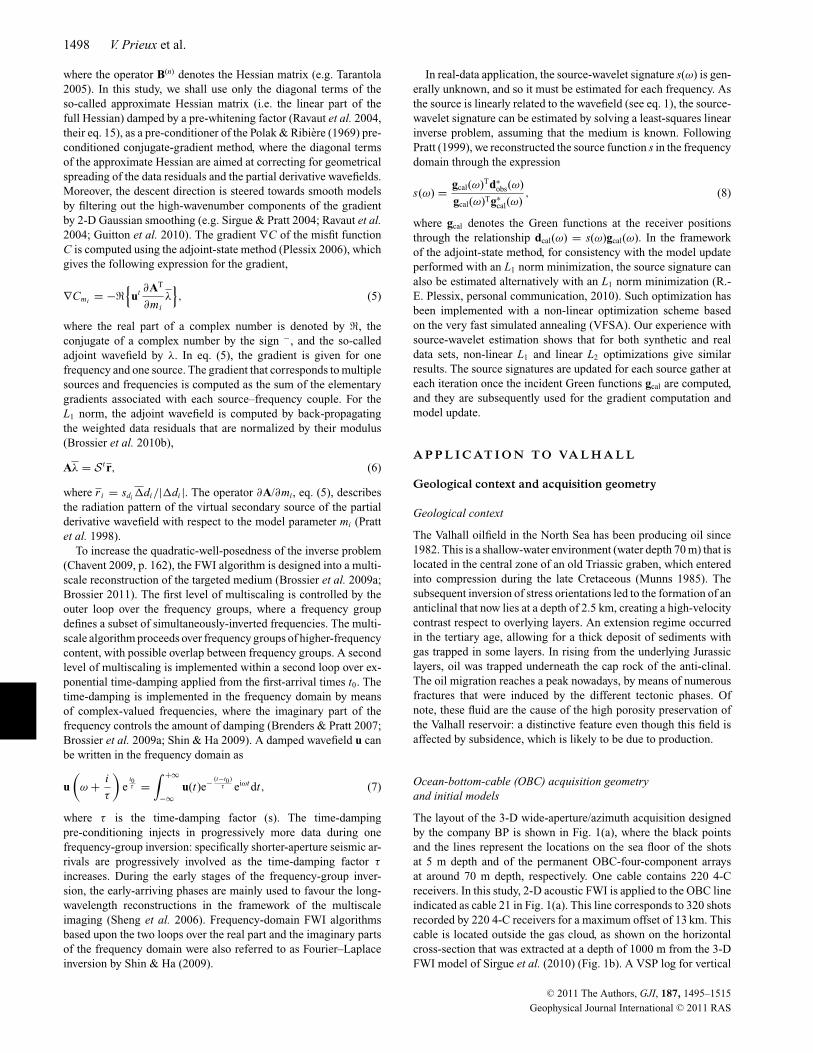
Figure 2. Two-dimensional sections along position of cable 21 through anisotropic 3-D models of the Valhall field. (a) Vertical velocity (V 0), (b) Thomsenparameter ε, (c) Thomsen parameter δ, (d) anellipticity parameter η, (e) density ρ, (f) NMO velocity (V NMO), (g) horizontal velocity (V h) and (h) horizontalvelocity updated by the first-arrival traveltime tomography (FATT model). The V 0, δ and ε models were built by reflection tomography (courtesy of BP). Thedensity model was inferred from the V NMO model using the Gardner law.

velocity is available on line 21 and it will be used to locally assessthe FWI results (Fig. 1c). A low-velocity zone that results from thepresence of gas layers is clearly seen on the VSP log, between 1.5and 2.5 km in depth.

A 3-D model for the vertical velocity V 0 and the Thomsen param-eters δ and ε (Thomsen 1986) has been developed by anisotropicreflection traveltime tomography in VTI media, and is providedby BP (Figs 2a–c). The vertical velocity model shows the low-velocity zone associated with the gas layers between 1.5 and 2.5 kmin depth, above the reservoir level (Fig. 2a). The correspondingnormal moveout (NMO) and horizontal velocity models are shownin Figs 2(f–g). In this study, by NMO velocity is meant the wavespeed given by VNMO = V0

√1 + 2δ (Tsvankin 1995), whereas the

horizontal velocity is given by Vh = V0

√1 + 2ε = VNMO

√1 + 2η,

respectively, where the anellipticity coefficient η is given by η =(ε − δ)/(1 + 2δ) (Alkhalifah & Tsvankin 1995). The NMO velocitiesshould allow the short-spread reflection traveltimes in VTI mediato be matched (Tsvankin 2001), whereas the horizontal velocitiesshould allow the refraction and long-spread reflection traveltimes tobe matched. Both velocity models can be viewed as initial models ofisotropic FWI of wide-aperture seismic data, as both short-aperturereflections and diving waves are recorded by long-offset acquisi-tion and are involved in this FWI processing. The 3-D FWI modeldeveloped by Sirgue et al. (2010) is obtained using the NMO veloc-ity model as the initial model (L. Sirgue, personal communication,2010). The percentage of the anisotropy in Valhall is shown by η ≈(V h − V NMO)/(V NMO), and it reaches a maximum value of 16 percent (Fig. 2d).

Anatomy of the data and starting-model appraisal

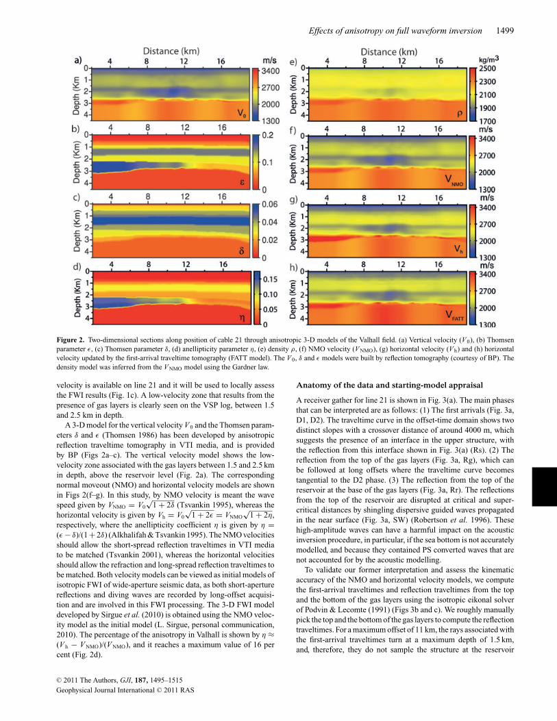
A receiver gather for line 21 is shown in Fig. 3(a). The main phasesthat can be interpreted are as follows: (1) The first arrivals (Fig. 3a,D1, D2). The traveltime curve in the offset-time domain shows twodistinct slopes with a crossover distance of around 4000 m, whichsuggests the presence of an interface in the upper structure, withthe reflection from this interface shown in Fig. 3(a) (Rs). (2) Thereflection from the top of the gas layers (Fig. 3a, Rg), which canbe followed at long offsets where the traveltime curve becomestangential to the D2 phase. (3) The reflection from the top of thereservoir at the base of the gas layers (Fig. 3a, Rr). The reflectionsfrom the top of the reservoir are disrupted at critical and super-critical distances by shingling dispersive guided waves propagatedin the near surface (Fig. 3a, SW) (Robertson et al. 1996). Thesehigh-amplitude waves can have a harmful impact on the acousticinversion procedure, in particular, if the sea bottom is not accuratelymodelled, and because they contained PS converted waves that arenot accounted for by the acoustic modelling.

To validate our former interpretation and assess the kinematicaccuracy of the NMO and horizontal velocity models, we computethe first-arrival traveltimes and reflection traveltimes from the topand the bottom of the gas layers using the isotropic eikonal solverof Podvin & Lecomte (1991) (Figs 3b and c). We roughly manuallypick the top and the bottom of the gas layers to compute the reflectiontraveltimes. For a maximum offset of 11 km, the rays associated withthe first-arrival traveltimes turn at a maximum depth of 1.5 km,and, therefore, they do not sample the structure at the reservoir

C© 2011 The Authors, GJI, 187, 1495–1515



Figure 3. OBC data set. (a) Example of pre-processed recorded receiver gather, at position x = 14 100 m. The vertical axis is plotted with a reduction velocityof 2.5 km s−1. Phase nomenclature: D1, D2, diving waves; Rs, shallow reflection; Rgss/Rgls, short-spread and long-spread reflections from the top of the gas;Rrss/Rrls, short-spread and long-spread reflections from the top of the reservoir; SW, shingling waves. (b) Top panel: ray tracing in the NMO velocity modelfor the first arrival (white rays), and the reflections from the top of the gas (red) and the reservoir (blue). Top of the gas and the reservoirs are delineated by redand blue solid lines, respectively. Bottom panel: receiver gather shown in (a) with superimposed traveltime curves computed in the NMO model for these threephases. (c) As (b) for the V h model. (d) As (c) for the FATT model. See text for details.

level below the gas layers. This implies that the first 1.5-km of thestructure are constrained by both diving waves and reflected waves,whereas the deeper structure is mostly constrained by short-spreadreflected waves. Superimposition of the computed traveltime curveson the receiver gather shows that the NMO velocities do not allowthe traveltimes at long offsets of diving waves and the long-spreadreflection Rg to be matched (Fig. 3b). The mismatch between theobserved and computed first-arrival traveltimes reaches around 0.3 sat 11 km of offset. Cycle skipping artefacts will occur when thistraveltime error exceeds half the period of the signal, that is fora frequency as low as roughly 1.7 Hz. In the following, we usean initial frequency of 3.5 Hz for inversion, which allows for amaximum traveltime error of 0.14 s, which is reached for an offsetof the order of 6 km. We conclude that FWI might be affected bycycle skipping artefacts that result from the inversion of the divingwaves and long-spread reflection recorded at offsets greater than 6km, when the NMO velocity model is used as an initial model. Incontrast, the NMO velocity model is expected to make the short-spread reflection traveltimes of the phases Rg and Rr to be matched,that is supported by Fig. 3(b). Unlike the Rg phase, the NMO

velocity model reasonably predicts the slope of the long-spreadreflection traveltimes of the Rr phase. Indeed, the reflection-angleillumination of the reflectors decreases with depth, which shouldmake the reflection traveltime curve associated with the top of thereservoir less sensitive to anisotropy (i.e. the difference betweenvertical and horizontal velocities) within the recorded offset range.The horizontal velocity model allows for a much better agreementof the first-arrival traveltimes (Fig. 3c). The reflection traveltimes ofthe phase Rr computed in this model are lower than the traveltimescomputed in the NMO model. The mismatch between the NMOand horizontal velocity reflection traveltimes at zero offset is ofthe order of 0.075 and 0.1 s for the Rg and Rr phases, respectively.Assuming that the NMO traveltimes accurately predict the observedreflection traveltimes, it is worth mentioning that these traveltimemismatches remain below the cycle-skipping limit of 0.14 s becauseshort-offset reflection data involve fewer propagated wavelengthsthan long-spread reflections and diving waves. We might concludefrom this analysis that the horizontal velocity model should providea more suitable initial model than the NMO velocity model forisotropic FWI because the traveltime errors remains always below

C© 2011 The Authors, GJI, 187, 1495–1515



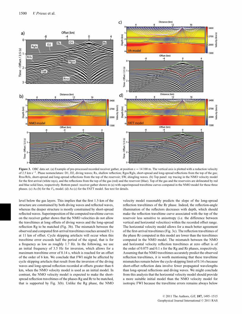
Figure 4. Seismic modelling. Close-up of the hybrid P1-P0 triangular mesh on which seismic modelling was performed using the DG method.

the cycle-skipping limit whatever the offsets. However, the NMOvelocity model is expected to provide the most accurate match ofthe short-aperture reflection traveltimes.

The horizontal-velocity model does not accurately match thefirst-arrival traveltimes at intermediate offsets (with a maximumerror of the order of 0.1 s at 5.5-km offset). This highlights thatseismic reflection data are not suitable for accurate reconstructionof horizontal velocities. This prompted us to update the horizontal-velocity model by FATT to improve the match of the first-arrivaltraveltimes before FWI (Figs 2h and 3d). This updated velocitymodel will be referred to as the FATT model in what follows.

In continuing this study, we use the NMO model and the FATTmodels as initial models for isotropic FWI, and we compare theisotropic FWI models with the results of anisotropic FWI for verticalvelocity.

FWI pre-processing and experimental setup

FWI pre-processing

Among the available 4-C receiver data, only the hydrophone com-ponent is considered as we are dealing with acoustic FWI. Acousticinversion was applied to the hydrophone component of the fully elas-tic data computed in the synthetic elastic Valhall model (Brossieret al. 2009b): a successful image of the V P structure has been ob-tained because converted P-SV waves have a minor footprint on thehydrophone component. Therefore, Valhall should provide a suit-able framework for the successful application of acoustic FWI toelastic data (see Barnes & Charara (2009), for a more general dis-cussion on the validity of the acoustic approximation in the marineenvironment). As the receivers are around 2/3-fold less numerousthan the shots, the data are sorted in receiver gathers by virtue of thesource–receiver reciprocity holding between an explosion sourceand a pressure component of the data, to reduce the computationalcost.

The FWI data pre-processing first consists of minimum-phasewhitening followed by Butterworth filtering of a [4–20] Hz band-width. The whitening is designed to preserve the geometricalspreading of the data, by normalizing the spectral amplitudes ofthe deconvolution operator associated with each trace according toits maximum amplitude. The bandwidth of the Butterworth filter ischosen heuristically to provide the best trade-off between the signal-to-noise ratio and the flattening of the amplitude spectrum. We thenapply FK filtering to remove as much S-wave energy as possible,and spectral matrix filtering (Mari et al. 1999, page 386) to enhancethe lateral coherency of events (Ravaut et al. 2004). We also applieda mute to remove noise before the first-arrival time, and after a timeof 4 s following the first-arrival excluding late arrivals. Finally, thedata are multiplied by the function

√t to roughly transform the 3-D

geometrical spreading of real amplitude data into a 2-D amplitudebehaviour. An example of a fully pre-processed receiver gather isshown in Fig. 3(a).

Experimental set-up: seismic modelling

The 18 000 × 5000 m velocity, density and attenuation models arediscretized on unstructured triangular meshes for seismic modellingwith the DG method, where the medium properties are piecewiseconstant per element (Brossier et al. 2008; Brossier 2011). Accuratepositioning of the seismic devices is allowed by the use of a finemesh in the first 160 m of the medium, where the linear interpolationorder (P1) is used to describe the acoustic wavefield (Fig. 4). Be-low, a regular triangular mesh is used with piecewise-constant (P0)representation of the wavefield in each cell to reduce the cost of themodelling in terms of memory and computation. A discretizationrule of 10 elements per wavelength is used in the regular mesh,which leads to 20-m-long triangle edges. The hybrid P1–P0 meshcontains around 585 × 103 cells. The mesh includes 500-m-thickperfectly matched layers on the right, left and bottom sides of themodel for the absorbing boundary conditions (Berenger 1994). Afree-surface boundary condition is implemented on top of the mod-els, which implies that free-surface multiples are involved duringthe FWI. Although the real depth of the receivers varies between 67and 73 m, we choose for convenience the design of a flat bathymetryat a depth of 70 m within the mesh: all receivers are put at a depthof 71 m, just below the sea bottom. This approximation has a minorimpact on the modelling accuracy given the shortest propagatedwavelength of 215 m.

Experimental set-up: inversion

Only the P-wave velocity is reconstructed during the inversion pro-cedure we perform. An attenuation model is set as homogeneousbelow the sea bottom to the realistic value of the attenuation factorQp = 150. This value of attenuation is chosen by trial-and-error,such that the root-mean-squares amplitudes of the early-arrivingphases computed in the initial model roughly matches those of therecorded data, following the approach of Pratt (1999, his Fig. 6).The density model is inferred from the starting FWI velocity mod-els using the Gardner law (Gardner et al. 1974) and is kept constantover iterations of the inversion (Fig. 2e).

We sequentially invert five increasing frequency groups between3.5 and 6.7 Hz ([3.5, 3.78, 4], [4, 4.3, 4.76], [4.76, 5, 5.25],[ 5.25,5.6, 6] and [6, 6.35, 6.7] Hz). We have verified that a sufficientlyhigh signal-to-noise ratio is inside the traces at the lowest frequencyof 3.5 Hz, as already used in the 3-D FWI application of Sirgue et al.(2010). The spectral amplitude of the 3.5-Hz frequency represents45 per cent of that of the dominant 7-Hz frequency after whitening

C© 2011 The Authors, GJI, 187, 1495–1515



and Butterworth filtering. The maximum frequency of 6.7 Hz issimilar to that used in Sirgue et al. (2010). We do not investigateyet whether the FWI can be pushed towards higher frequenciesfor this case study. We design our frequency groups with threefrequencies per group, with one-frequency overlapping between thegroups.

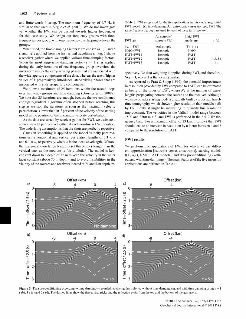
When used, the time-damping factors τ are chosen as 1, 3 and 5s, and were applied from the first-arrival traveltime t0. Fig. 5 showsa receiver gather where we applied various time-damping factors.When the most aggressive damping factor (τ = 1 s) is appliedduring the early iterations of one frequency-group inversion, theinversion favours the early-arriving phases that are associated withthe wide-aperture components of the data, whereas the use of highervalues of τ progressively introduces later-arriving phases that areassociated with shorter-aperture components.

We allow a maximum of 25 iterations within the nested loopsover frequency groups and time damping (Brossier et al. 2009a).We note that 25 iterations are enough, because the pre-conditionedconjugate-gradient algorithm often stopped before reaching thisstep as we stop the iterations as soon as the maximum velocityperturbation is lower that 10−3 per cent of the velocity of the startingmodel at the position of the maximum velocity perturbation.

As the data are sorted by receiver gather for FWI, we estimate asource wavelet per receiver gather at each non-linear FWI iteration.The underlying assumption is that the shots are perfectly repetitive.

Gaussian smoothing is applied to the model velocity perturba-tions using horizontal and vertical correlation lengths of 0.3 × λ

and 0.1 × λ, respectively, where λ is the local wavelength. Of note,the horizontal correlation length is set three-times longer than thevertical one, as the medium is fairly tabular. The model is keptconstant down to a depth of 77 m to keep the velocity in the waterlayer constant (above 70 m depth), and to avoid instabilities in thevicinity of the sources and receivers located at 71 and 5-m depth, re-

Table 1. FWI setup used for the five applications in this study; m0, initialFWI model; τ (s), time damping; A/I, anisotropic versus isotropic FWI. Thesame frequency groups are used for each of these tests (see text).

Anisotropic/ Initial FWIFWI test isotropic FWI model m0 τ (s)

V 0 + FWI Anisotropic (V 0, δ, ε) –NMO+FWI Isotropic NMO –FATT+FWI 1 Isotropic FATT –FATT+FWI 2 Isotropic FATT 1, 3, 5 sFATT+FWI 3 Isotropic FATT 1 s

spectively. No data weighting is applied during FWI, and, therefore,Wd = I, where I is the identity matrix.

As reported by Pratt & Shipp (1999), the potential improvementin resolution provided by FWI compared to FATT, can be estimatedas being of the order of

√Nλ, where Nλ is the number of wave-

lengths propagating between the source and the receiver. Althoughwe also consider starting models originally built by reflection travel-time tomography, which shows higher resolution than models builtby FATT only, it might be interesting to quantify this resolutionimprovement. The velocities in the Valhall model range between1500 and 3500 m s−1, and FWI is performed in the 3.5–7 Hz fre-quency band. For a maximum offset of 13 km, it follows that FWIshould lead to an increase in resolution by a factor between 4 and 8compared to the resolution of FATT.

FWI results

We perform five applications of FWI, for which we use differ-ent approximation [isotropic versus anisotropic], starting models((V 0,δ,ε), NMO, FATT models), and data pre-conditioning (with-out and with time dampings). The main features of the five inversionapplications are outlined in Table 1.

Figure 5. Data pre-conditioning according to time damping—recorded receiver gathers plotted without time damping (a), and with time damping using τ = 1s (b), 3 s (c) and 5 s (d). The dashed lines show the first-arrival picks and the reflection picks from the top and the bottom of the gas layers.

C© 2011 The Authors, GJI, 187, 1495–1515



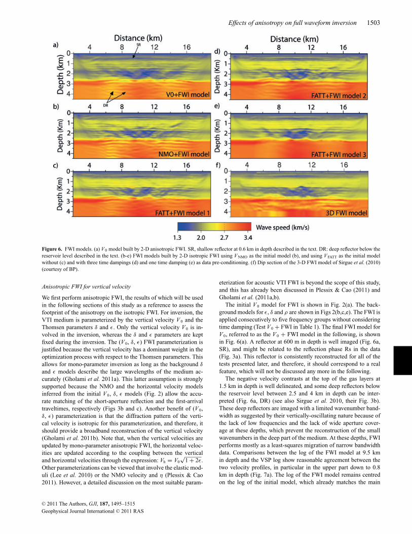
Figure 6. FWI models. (a) V 0 model built by 2-D anisotropic FWI. SR, shallow reflector at 0.6 km in depth described in the text. DR: deep reflector below thereservoir level described in the text. (b-e) FWI models built by 2-D isotropic FWI using V NMO as the initial model (b), and using V FATT as the initial modelwithout (c) and with three time dampings (d) and one time damping (e) as data pre-conditioning. (f) Dip section of the 3-D FWI model of Sirgue et al. (2010)(courtesy of BP).

Anisotropic FWI for vertical velocity

We first perform anisotropic FWI, the results of which will be usedin the following sections of this study as a reference to assess thefootprint of the anisotropy on the isotropic FWI. For inversion, theVTI medium is parameterized by the vertical velocity V 0 and theThomsen parameters δ and ε. Only the vertical velocity V 0 is in-volved in the inversion, whereas the δ and ε parameters are keptfixed during the inversion. The (V 0, δ, ε) FWI parameterization isjustified because the vertical velocity has a dominant weight in theoptimization process with respect to the Thomsen parameters. Thisallows for mono-parameter inversion as long as the background δ

and ε models describe the large wavelengths of the medium ac-curately (Gholami et al. 2011a). This latter assumption is stronglysupported because the NMO and the horizontal velocity modelsinferred from the initial V 0, δ, ε models (Fig. 2) allow the accu-rate matching of the short-aperture reflection and the first-arrivaltraveltimes, respectively (Figs 3b and c). Another benefit of (V 0,δ, ε) parameterization is that the diffraction pattern of the verti-cal velocity is isotropic for this parameterization, and therefore, itshould provide a broadband reconstruction of the vertical velocity(Gholami et al. 2011b). Note that, when the vertical velocities areupdated by mono-parameter anisotropic FWI, the horizontal veloc-ities are updated according to the coupling between the verticaland horizontal velocities through the expression: Vh = V0

√1 + 2ε.

Other parameterizations can be viewed that involve the elastic mod-uli (Lee et al. 2010) or the NMO velocity and η (Plessix & Cao2011). However, a detailed discussion on the most suitable param-

eterization for acoustic VTI FWI is beyond the scope of this study,and this has already been discussed in Plessix & Cao (2011) andGholami et al. (2011a,b).

The initial V 0 model for FWI is shown in Fig. 2(a). The back-ground models for ε, δ and ρ are shown in Figs 2(b,c,e). The FWI isapplied consecutively to five frequency groups without consideringtime damping (Test V 0 + FWI in Table 1). The final FWI model forV 0, referred to as the V 0 + FWI model in the following, is shownin Fig. 6(a). A reflector at 600 m in depth is well imaged (Fig. 6a,SR), and might be related to the reflection phase Rs in the data(Fig. 3a). This reflector is consistently reconstructed for all of thetests presented later, and therefore, it should correspond to a realfeature, which will not be discussed any more in the following.

The negative velocity contrasts at the top of the gas layers at1.5 km in depth is well delineated, and some deep reflectors belowthe reservoir level between 2.5 and 4 km in depth can be inter-preted (Fig. 6a, DR) (see also Sirgue et al. 2010, their Fig. 3b).These deep reflectors are imaged with a limited wavenumber band-width as suggested by their vertically-oscillating nature because ofthe lack of low frequencies and the lack of wide aperture cover-age at these depths, which prevent the reconstruction of the smallwavenumbers in the deep part of the medium. At these depths, FWIperforms mostly as a least-squares migration of narrow bandwidthdata. Comparisons between the log of the FWI model at 9.5 kmin depth and the VSP log show reasonable agreement between thetwo velocity profiles, in particular in the upper part down to 0.8km in depth (Fig. 7a). The log of the FWI model remains centredon the log of the initial model, which already matches the main

C© 2011 The Authors, GJI, 187, 1495–1515



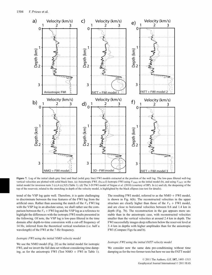
Figure 7. Log of the initial (dash grey line) and final (solid grey line) FWI models extracted at the position of the well log. The low-pass filtered well-logvertical velocities are plotted with solid black lines. (a) Anisotropic FWI. (b,c,e,f) Isotropic FWI using V NMO as the initial model (b), and using V FATT as theinitial model for inversion tests 3 (c),4 (e),5(f) (Table 1). (d) The 3-D FWI model of Sirgue et al. (2010) (courtesy of BP). In (c) and (d), the deepening of thetop of the reservoir, related to the stretching in depth of the velocity model, is highlighted by the black ellipses (see text for details).

trend of the VSP log quite well. Therefore, it is quite challengingto discriminate between the true features of the FWI log from theartificial ones. Rather than assessing the match of the V 0 FWI logwith the VSP log in an absolute sense, we shall rather use the com-parison between the V 0 + FWI log and the VSP log as a reference tohighlight the differences with the isotropic FWI results presented inthe following. Of note, the VSP log is low-pass filtered in the timedomain after depth-to-time conversion with a cut-off frequency of14 Hz, inferred from the theoretical vertical resolution (i.e. half awavelength) of the FWI at the 7-Hz frequency.

Isotropic FWI using the initial NMO velocity model

We use the NMO model (Fig. 2f) as the initial model for isotropicFWI, and we invert the full data set without considering time damp-ing, as for the anisotropic FWI (Test NMO + FWI in Table 1).

The resulting FWI model, referred to as the NMO + FWI model,is shown in Fig. 6(b). The reconstructed velocities in the upperstructure are clearly higher than those of the V 0 + FWI model,and are close to horizontal velocities between 0.6 and 1.4 km indepth (Fig. 7b). The reconstruction in the gas appears more un-stable than in the anisotropic case, with reconstructed velocitiessmaller than the vertical velocities at around 2.4 km in depth. TheFWI successfully images deep reflectors below the reservoir level at3–4 km in depths with higher amplitudes than for the anisotropicFWI (Compare Figs 6a and b).

Isotropic FWI using the initial FATT velocity model

We consider now the same data pre-conditioning without timedamping as for the two former tests but here we use the FATT model

C© 2011 The Authors, GJI, 187, 1495–1515



as the initial model for the isotropic FWI (Test FATT + FWI 1 inTable 1). The resulting FWI model, which is referred to as the FATT+ FWI model 1, is shown in Fig. 6(c). Compared to the NMO +FWI model, the FATT + FWI model 1 has slightly higher velocitiesbetween 0.6 and 1.6 km in depth, that highlights the footprint on theinitial model (Fig. 7c). These velocities remained centered aroundthe horizontal velocities of the initial model at these depths. Thevelocities within the gas layers between 2 and 2.5 km in depth areclose to the vertical velocities along the well, and are higher thanthose of the NMO + FWI model. We note also a high-velocity per-turbation at 3 km in depth, where the velocity reaches a maximumvalue of 3.3 km s−1 (Fig. 7b). This velocity perturbation is absent inthe NMO + FWI model, where the maximum velocity is reached ata depth of 2.7 km (Fig. 7b). This deep velocity perturbation mightindicate a vertical stretching of the deep structure to balance thehigh horizontal velocities reconstructed in the upper structure, andthe velocities in the gas layers higher than those of the NMO model.

During a second test with the FATT model, we use three timedampings in cascade during the inversion of each frequency group(τ = 1, 3, 5 s) (Test FATT + FWI 2 in Table 1). Note that thewide-aperture components associated with strong time dampingsare injected first during one frequency group. On one hand, thisis consistent as these aperture components are those that are ac-curately predicted by the starting FATT model. On the other hand,this hierarchical strategy is consistent with the multiscale approach,where the long wavelengths constrained by the wide apertures mustbe first reconstructed. The final FWI model, referred to as FATT +FWI model 2, is shown in Fig. 6(d). As for the FATT + FWI model1, the horizontal velocities are mainly reconstructed down to 1.5km in depth, where the top of the gas layers is well delineated by asharp negative velocity contrast (Fig. 7e). Overall, the velocities inthe gas are lower than the vertical velocities along the well below1.8 km in depth. The maximum velocity at the reservoir level isreached at 2.7 km in depth as for the NMO model.

During the third test performed with the FATT model, we consideronly a time-damping factor of 1 s (Test FATT + FWI 3 in Table 1). Atime-damping factor of 1 s favours the aperture components of thedata which are well predicted by the FATT model from a kinematicviewpoint, and it heavily damps the contribution of the deep short-aperture reflections in the data. The final FWI model, referred to asFATT + FWI model 3, is shown in Fig. 6(e). The velocity structureof the FATT + FWI model 3 is similar to the one of the FATT + FWImodel 2. However, the velocities in the gas are in overall lower andthe deep part of the model is less perturbed and shows a smootherpattern due to the use of a more limited subdataset during inversion(compare Figs 7e and f).

For possible identification of artefacts relating to the 3-D prop-agation effects, we show the dip section of the 3-D isotropic FWImodel of Sirgue et al. (2010) along cable 21 (Fig. 6f). Interestingly,the velocities above the gas between 0.5 and 1.5 km in depth arequite close to those of the FATT + FWI model 1 (compare Figs 7dand c). The vertical stretching between 2.5 and 3 km in depth ofthe 3-D FWI model might have a similar origin than the one hy-pothesized for the FATT + FWI model 1 (compare Figs 7c and d).The consistency between the dip section of the 3-D FWI model ofSirgue et al. (2010) and the FATT + FWI model 1 strongly supportsthat 3-D effects have a minor impact on the 2-D FWI results.

Model appraisals

Model appraisal is a key issue in FWI as uncertainty analysis is quitechallenging to perform in a Bayesian framework (Gouveia & Scales

1998). In this study, the FWI models are evaluated based upon fourcriteria: the local match with the VSP log, the flatness of the commonimage gathers (CIG) computed by RTM, the synthetic seismogrammodelling, and the repeatability of source-wavelet estimation.

Reverse time migration and common image gathers

We compute 2-D RTM and CIGs in the offset-depth domain. RTMis performed in the frequency domain using the acoustic VTI finite-difference frequency-domain modelling method of Operto et al.(2009) and the gradient of the FWI program of Sourbier et al.(2009a,b), where the data residuals are replaced by the data. Each ofthe common-offset migrated images was computed independentlyto generate CIGs before stacking. The range of offsets that is con-sidered for migration ranges from −5 to 5 km. For migration, weuse a suitable pre-processed data set, where free-surface multiplesare removed. The migrated images are displayed with an automaticgain control.

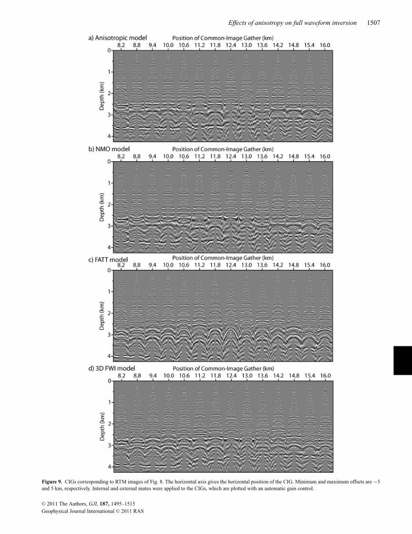
The anisotropic RTM performed in the initial (V 0, δ, ε) modelprovides a good image of the subsurface, with a good continuity ofthe top of the reservoir beneath the gas layers at 2.5 km in depth andof a deep reflector between 3 and 3.5 km in depth (Fig. 8a, DR) (seealso Fig. 3 in Sirgue et al. (2010)). The quality of the anisotropicmigrated image is further confirmed by the overall flatness of thereflectors in the CIGs (Fig. 9a). The isotropic RTM computed inthe NMO model produces an acceptable image, although the imageof the top of the reservoir is slightly less focused than the one ob-tained by anisotropic RTM (Fig. 8b). The deep reflector below thereservoir level is shifted downwards by around 250 m with respectto its position in the anisotropic image because the NMO migra-tion velocities in isotropic RTM are on average faster than thoseof anisotropic RTM when short-spread data are considered. On theother hand, the reflectors are slightly smiling in the CIGs, whichsuggest too slow velocities at long offsets (Fig. 9b). The migratedimage computed in the FATT model shows a severe misfocusingof the top of the reservoir with a significant deepening of the deepreflector below the reservoir level, due to the high migration veloc-ities associated with horizontal velocities (Fig. 8c). These too highvelocities are clearly highlighted by frowning reflectors in the CIGs(Fig. 9c).

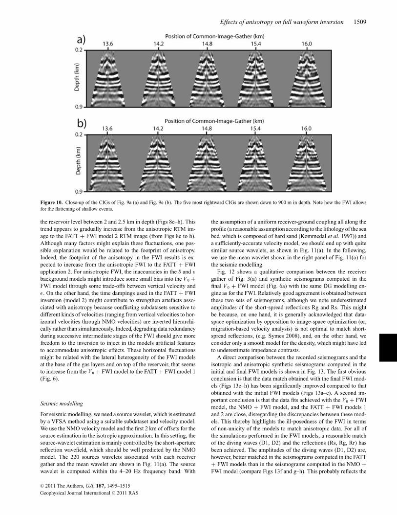
The migrated images computed in the FWI models are shown inFigs 8(e–h). Overall, the anisotropic FWI model does not allow usto improve the RTM image of the deep structure obtained from theanisotropic reflection traveltime tomography (compare Figs 8a ande). This is, to some extent, expected because the workflow, whichcombines the traveltime reflection tomography (or, migration-basedvelocity analysis) with the RTM, is more consistent than the onecombining FWI with RTM. In the first case, the same subset of data,that is the short-spread reflections, is used during both the velocitymodel building and RTM, and the scale separation underlying thesetwo tasks contributes to make the workflow well posed. In contrast,the FWI is a more ill-posed problem, where significant errors canbe propagated in depth as longer offsets are processed. We note,however, that the reflectors in the CIGs inferred from the FWImodel are significantly flatter in the shallow part (the first 1 km)than the ones inferred from the anisotropic reflection traveltimetomography model (Fig. 10). This highlights the capability of FWIfor exploiting shallow reflections over the full aperture range, unlikereflection traveltime tomography. The improvement in the imagingof the shallow structure is observed for all of the migration testsdescribed later. The NMO + FWI model produces CIGs, for whichthe smiling effects are slightly reduced (compare Figs 9b and f).

C© 2011 The Authors, GJI, 187, 1495–1515



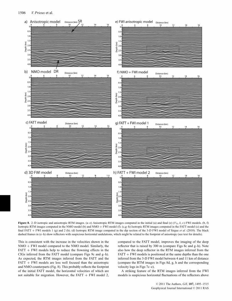
Figure 8. 2–D isotropic and anisotropic RTM images. (a–e) Anisotropic RTM images computed in the initial (a) and final (e) (V 0, δ, ε) FWI models. (b, f)Isotropic RTM images computed in the NMO model (b) and NMO + FWI model (f). (c,g–h) Isotropic RTM images computed in the FATT model (c) and thefinal FATT + FWI models 1 (g) and 2 (h). (d) Isotropic RTM image computed in the dip section of the 3-D FWI model of Sirgue et al. (2010). The blackdashed frames in (e–h) show reflectors with suspicious horizontal undulations, which might be related to the footprint of anisotropy (see text for details).

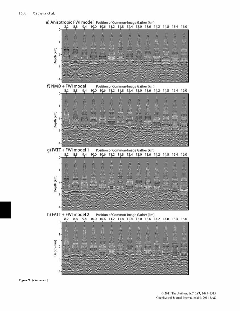
This is consistent with the increase in the velocities shown in theNMO + FWI model compared to the NMO model. Similarly, theFATT + FWI models help to reduce the frowning effects in theCIGs inferred from the FATT model (compare Figs 9c and g–h).As expected, the RTM images inferred from the FATT and theFATT + FWI models are less well focused than the anisotropicand NMO counterparts (Fig. 8). This probably reflects the footprintof the initial FATT model, the horizontal velocities of which arenot suitable for migration. However, the FATT + FWI model 2,

compared to the FATT model, improves the imaging of the deepreflector that is raised by 300 m (compare Figs 8c and g–h). Notealso how the deep reflector in the RTM images inferred from theFATT + FWI models is positioned at the same depths than the oneinferred from the 3-D FWI model between 4 and 11 km of distance(compare the RTM images in Figs 8d, g, h and the correspondingvelocity logs in Figs 7c–e).

A striking feature of the RTM images inferred from the FWImodels is suspicious horizontal fluctuations of the reflectors above

C© 2011 The Authors, GJI, 187, 1495–1515



Figure 9. CIGs corresponding to RTM images of Fig. 8. The horizontal axis gives the horizontal position of the CIG. Minimum and maximum offsets are −5and 5 km, respectively. Internal and external mutes were applied to the CIGs, which are plotted with an automatic gain control.

C© 2011 The Authors, GJI, 187, 1495–1515



Figure 9. (Continued.)

C© 2011 The Authors, GJI, 187, 1495–1515



Figure 10. Close-up of the CIGs of Fig. 9a (a) and Fig. 9e (b). The five most rightward CIGs are shown down to 900 m in depth. Note how the FWI allowsfor the flattening of shallow events.

the reservoir level between 2 and 2.5 km in depth (Figs 8e–h). Thistrend appears to gradually increase from the anisotropic RTM im-age to the FATT + FWI model 2 RTM image (from Figs 8e to h).Although many factors might explain these fluctuations, one pos-sible explanation would be related to the footprint of anisotropy.Indeed, the footprint of the anisotropy in the FWI results is ex-pected to increase from the anisotropic FWI to the FATT + FWIapplication 2. For anisotropic FWI, the inaccuracies in the δ and ε

background models might introduce some small bias into the V 0 +FWI model through some trade-offs between vertical velocity andε. On the other hand, the time dampings used in the FATT + FWIinversion (model 2) might contribute to strengthen artefacts asso-ciated with anisotropy because conflicting subdatasets sensitive todifferent kinds of velocities (ranging from vertical velocities to hor-izontal velocities through NMO velocities) are inverted hierarchi-cally rather than simultaneously. Indeed, degrading data redundancyduring successive intermediate stages of the FWI should give morefreedom to the inversion to inject in the models artificial featuresto accommodate anisotropic effects. These horizontal fluctuationsmight be related with the lateral heterogeneity of the FWI modelsat the base of the gas layers and on top of the reservoir, that seemsto increase from the V 0 + FWI model to the FATT + FWI model 1(Fig. 6).

Seismic modelling

For seismic modelling, we need a source wavelet, which is estimatedby a VFSA method using a suitable subdataset and velocity model.We use the NMO velocity model and the first 2 km of offsets for thesource estimation in the isotropic approximation. In this setting, thesource-wavelet estimation is mainly controlled by the short-aperturereflection wavefield, which should be well predicted by the NMOmodel. The 220 sources wavelets associated with each receivergather and the mean wavelet are shown in Fig. 11(a). The sourcewavelet is computed within the 4–20 Hz frequency band. With

the assumption of a uniform receiver-ground coupling all along theprofile (a reasonable assumption according to the lithology of the seabed, which is composed of hard sand (Kommedal et al. 1997)) anda sufficiently-accurate velocity model, we should end up with quitesimilar source wavelets, as shown in Fig. 11(a). In the following,we use the mean wavelet shown in the right panel of Fig. 11(a) forthe seismic modelling.

Fig. 12 shows a qualitative comparison between the receivergather of Fig. 3(a) and synthetic seismograms computed in thefinal V 0 + FWI model (Fig. 6a) with the same DG modelling en-gine as for the FWI. Relatively good agreement is obtained betweenthese two sets of seismograms, although we note underestimatedamplitudes of the short-spread reflections Rg and Rs. This mightbe because, on one hand, it is generally acknowledged that data-space optimization by opposition to image-space optimization (or,migration-based velocity analysis) is not optimal to match short-spread reflections, (e.g. Symes 2008), and, on the other hand, weconsider only a smooth model for the density, which might have ledto underestimate impedance contrasts.

A direct comparison between the recorded seismograms and theisotropic and anisotropic synthetic seismograms computed in theinitial and final FWI models is shown in Fig. 13. The first obviousconclusion is that the data match obtained with the final FWI mod-els (Figs 13e–h) has been significantly improved compared to thatobtained with the initial FWI models (Figs 13a–c). A second im-portant conclusion is that the data fits achieved with the V 0 + FWImodel, the NMO + FWI model, and the FATT + FWI models 1and 2 are close, disregarding the discrepancies between these mod-els. This thereby highlights the ill-posedness of the FWI in termsof non-unicity of the models to match anisotropic data. For all ofthe simulations performed in the FWI models, a reasonable matchof the diving waves (D1, D2) and the reflections (Rs, Rg, Rr) hasbeen achieved. The amplitudes of the diving waves (D1, D2) are,however, better matched in the seismograms computed in the FATT+ FWI models than in the seismograms computed in the NMO +FWI model (compare Figs 13f and g–h). This probably reflects the

C© 2011 The Authors, GJI, 187, 1495–1515



Figure 11. Source-wavelets estimation. (a) Using isotropic modeling for a maximum offset of 2 km and the NMO velocity model. (b, f) Using anisotropicmodeling for the full offset range and the initial (b) and final (f) (V 0, δ, ε) FWI models. (c, g) Using isotropic modeling and the NMO model (c) and NMO +FWI models (g). (d, h) As (c, g) for the FATT model (d) and the FATT + FWI model 1 (h). (e) Using isotropic modeling for the full offset range and the dipsection of the 3D FWI model of Sirgue et al. (2010). Note the improved focusing of the wavelets when using the FWI models.

kinematic accuracy of the FATT model to match first-arrival trav-eltimes. However, the seismograms computed in the NMO + FWImodel do not show obvious evidence of cycle skipping artefactsat large offsets for the diving waves, as the first-arrival traveltimescomputed in the NMO + FWI model accurately match the observedfirst-arrival traveltimes (Fig. 13f). The match of the first arrivals isconsistent with our showing that the FWI converged towards veloci-ties close to the horizontal velocities in the upper structure when theNMO model is used as the initial model (Fig. 7b). The successfulmatch of the diving waves recorded at long offsets is unexpectedwhen the NMO model is used as the initial FWI model because thetraveltime mismatch between the recorded and the computed first-arrival traveltimes (0.3 s) exceeds the cycle-skipping limit at longoffsets for a starting frequency of 3.5 Hz. This successful matchcan be interpreted on the basis that the FWI has performed a hierar-chical layer-stripping reconstruction of the velocity structure overiterations, where the shallow part of the medium constrained bythe high-amplitude short-offset early arrivals are reconstructed firstfollowed by the reconstruction of the deeper part. This hierarchicalreconstruction of the velocity structure according to depth mighthave contributed to the progressive absorption of the traveltimemisfit with the offset, as the shallow part of the medium is improvedby the FWI. The match of the short-spread reflection phases is al-most equivalent in all of the seismograms, which is consistent withthe concept that all of the initial models allow the prediction of thetraveltimes within the cycle-skipping limit.

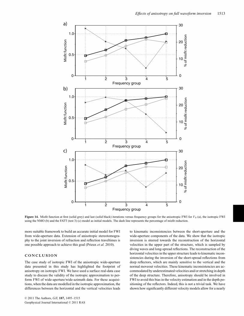
The data match is also shown by the plot of the misfit functions atthe first and last FWI iterations as a function of the frequency group.The curves show essentially similar trends for the anisotropic FWIand the isotropic FWI using the NMO and FATT models as initialmodels (Fig. 14).

Source-wavelet estimation as a tool for model appraisal

We use the source-wavelet estimation as a tool to appraise the rel-evance of the FWI models (Jaiswal et al. 2009). We estimate thesource wavelets by considering the full offset range, to make thewavelet estimation more sensitive to the model quality (Fig. 11).

The sensitivity of the wavelet estimation to the amount of data usedin eq. (8) can be assessed by comparing the wavelets estimated inthe NMO model using maximum offsets of 2000 m (Fig. 11a) and13 000 m (Fig. 11c). If the velocity model is not accurate enough, therepeatability of the wavelets is strongly affected when all of the aper-ture components of the data are involved in the inversion process.The collection of the source wavelets and the corresponding meanwavelet inferred from the initial and final FWI models when the fulloffset range is involved in the estimation is shown in Figs 11(b–d)and (f–h). Comparisons between the wavelets computed in the ini-tial and the final FWI models show how the source-wavelet esti-mation is improved when a FWI model is used, hence validatingthe relevance of the FWI results. The wavelet inferred from the dipsection of the 3D FWI model of Sirgue et al. (2010) is shown inFig. 11(e). This has a similar shape and amplitude to that obtained by2D FWI.

D I S C U S S I O N

We have presented here the application of VTI anisotropic andisotropic acoustic FWI to wide-aperture OBC data from the Valhallfield. We used both NMO and FATT models as initial models forthe isotropic FWI, where the FATT model roughly represents thehorizontal velocities of the VTI medium. The results highlight thefootprint of anisotropy on isotropic FWI.

Although there are significant differences between the kinematicproperties of the initial models we used, the final isotropic FWImodels show some overall common features. The most obvious oneis that the horizontal velocities are mainly reconstructed in the upperstructure, whatever the initial model and the data pre-conditioning.Therefore, the isotropic velocities in the upper structure are sig-nificantly higher than the velocities reconstructed by the mono-parameter anisotropic FWI for the vertical velocity. The horizontalvelocities are also reconstructed in the 3-D isotropic FWI modelof Sirgue et al. (2010), and, therefore they cannot be interpreted asthe footprint of the 3D effects. The reconstruction of the horizon-tal velocities in the upper structure shows that the FWI imaging is

C© 2011 The Authors, GJI, 187, 1495–1515



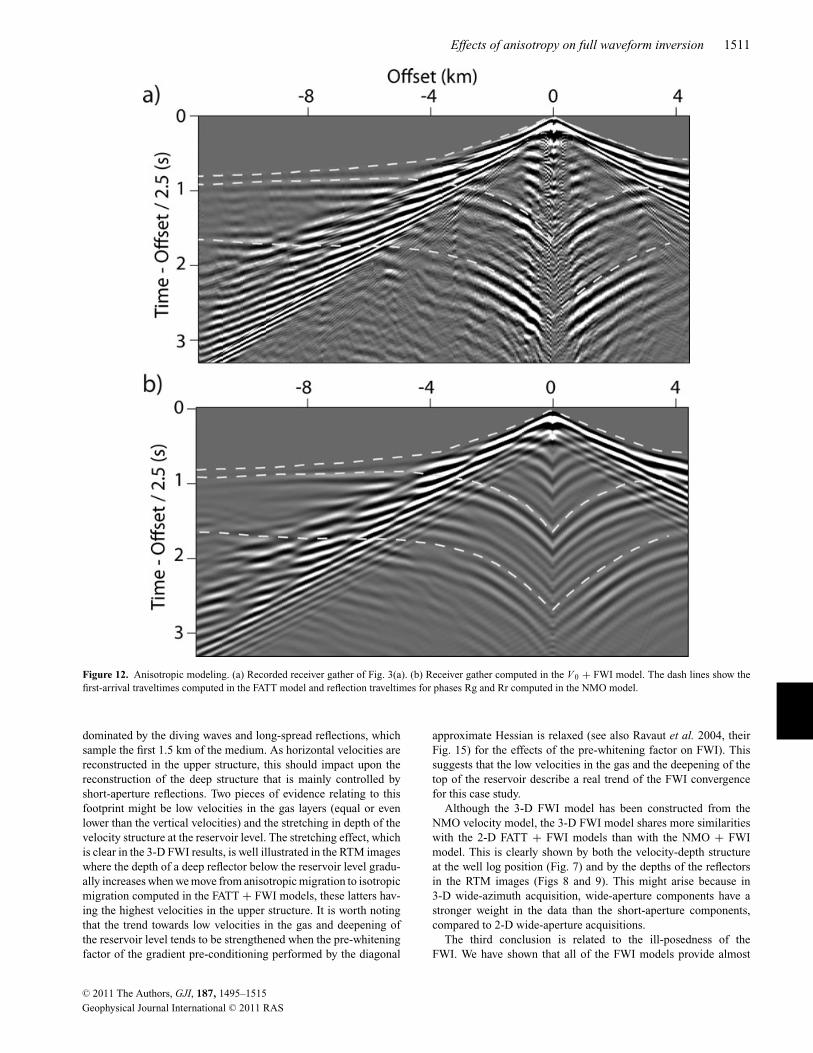
Figure 12. Anisotropic modeling. (a) Recorded receiver gather of Fig. 3(a). (b) Receiver gather computed in the V 0 + FWI model. The dash lines show thefirst-arrival traveltimes computed in the FATT model and reflection traveltimes for phases Rg and Rr computed in the NMO model.

dominated by the diving waves and long-spread reflections, whichsample the first 1.5 km of the medium. As horizontal velocities arereconstructed in the upper structure, this should impact upon thereconstruction of the deep structure that is mainly controlled byshort-aperture reflections. Two pieces of evidence relating to thisfootprint might be low velocities in the gas layers (equal or evenlower than the vertical velocities) and the stretching in depth of thevelocity structure at the reservoir level. The stretching effect, whichis clear in the 3-D FWI results, is well illustrated in the RTM imageswhere the depth of a deep reflector below the reservoir level gradu-ally increases when we move from anisotropic migration to isotropicmigration computed in the FATT + FWI models, these latters hav-ing the highest velocities in the upper structure. It is worth notingthat the trend towards low velocities in the gas and deepening ofthe reservoir level tends to be strengthened when the pre-whiteningfactor of the gradient pre-conditioning performed by the diagonal

approximate Hessian is relaxed (see also Ravaut et al. 2004, theirFig. 15) for the effects of the pre-whitening factor on FWI). Thissuggests that the low velocities in the gas and the deepening of thetop of the reservoir describe a real trend of the FWI convergencefor this case study.

Although the 3-D FWI model has been constructed from theNMO velocity model, the 3-D FWI model shares more similaritieswith the 2-D FATT + FWI models than with the NMO + FWImodel. This is clearly shown by both the velocity-depth structureat the well log position (Fig. 7) and by the depths of the reflectorsin the RTM images (Figs 8 and 9). This might arise because in3-D wide-azimuth acquisition, wide-aperture components have astronger weight in the data than the short-aperture components,compared to 2-D wide-aperture acquisitions.

The third conclusion is related to the ill-posedness of theFWI. We have shown that all of the FWI models provide almost

C© 2011 The Authors, GJI, 187, 1495–1515



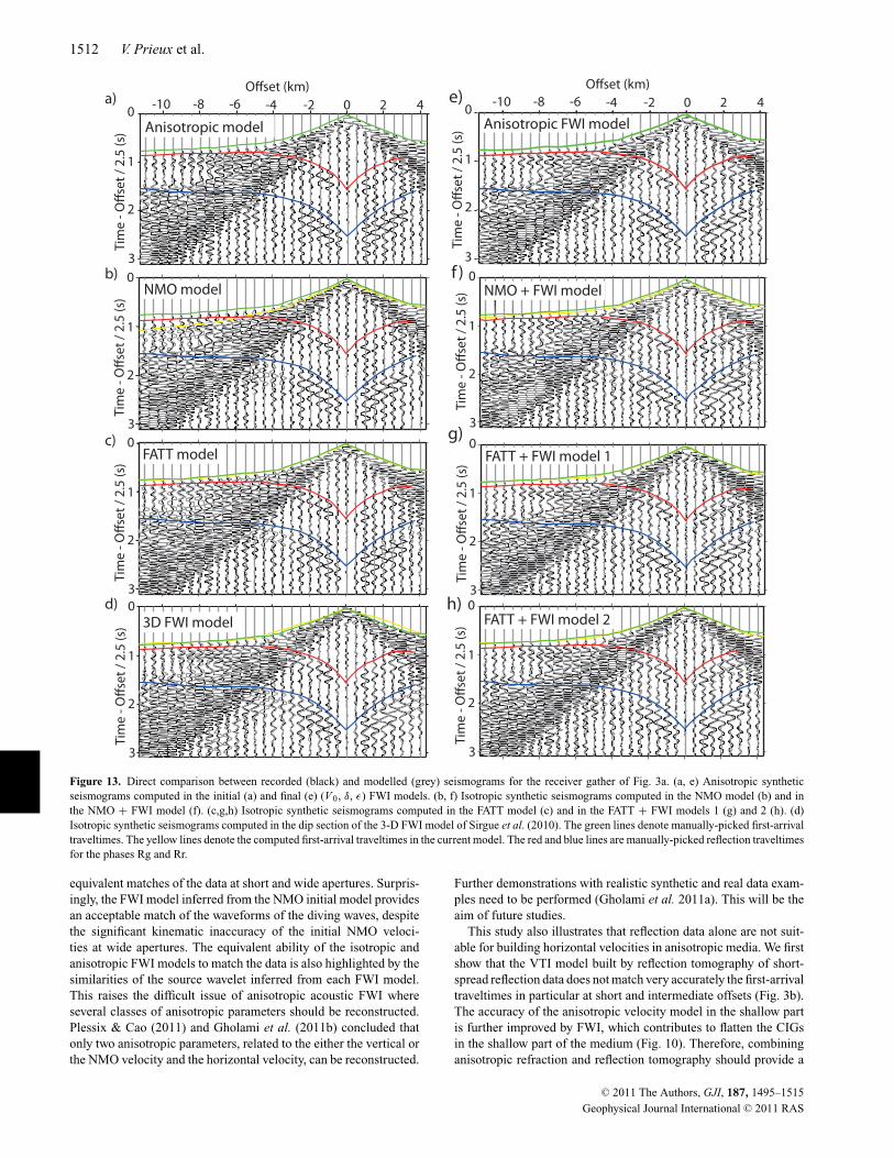
Figure 13. Direct comparison between recorded (black) and modelled (grey) seismograms for the receiver gather of Fig. 3a. (a, e) Anisotropic syntheticseismograms computed in the initial (a) and final (e) (V 0, δ, ε) FWI models. (b, f) Isotropic synthetic seismograms computed in the NMO model (b) and inthe NMO + FWI model (f). (c,g,h) Isotropic synthetic seismograms computed in the FATT model (c) and in the FATT + FWI models 1 (g) and 2 (h). (d)Isotropic synthetic seismograms computed in the dip section of the 3-D FWI model of Sirgue et al. (2010). The green lines denote manually-picked first-arrivaltraveltimes. The yellow lines denote the computed first-arrival traveltimes in the current model. The red and blue lines are manually-picked reflection traveltimesfor the phases Rg and Rr.

equivalent matches of the data at short and wide apertures. Surpris-ingly, the FWI model inferred from the NMO initial model providesan acceptable match of the waveforms of the diving waves, despitethe significant kinematic inaccuracy of the initial NMO veloci-ties at wide apertures. The equivalent ability of the isotropic andanisotropic FWI models to match the data is also highlighted by thesimilarities of the source wavelet inferred from each FWI model.This raises the difficult issue of anisotropic acoustic FWI whereseveral classes of anisotropic parameters should be reconstructed.Plessix & Cao (2011) and Gholami et al. (2011b) concluded thatonly two anisotropic parameters, related to the either the vertical orthe NMO velocity and the horizontal velocity, can be reconstructed.

Further demonstrations with realistic synthetic and real data exam-ples need to be performed (Gholami et al. 2011a). This will be theaim of future studies.

This study also illustrates that reflection data alone are not suit-able for building horizontal velocities in anisotropic media. We firstshow that the VTI model built by reflection tomography of short-spread reflection data does not match very accurately the first-arrivaltraveltimes in particular at short and intermediate offsets (Fig. 3b).The accuracy of the anisotropic velocity model in the shallow partis further improved by FWI, which contributes to flatten the CIGsin the shallow part of the medium (Fig. 10). Therefore, combininganisotropic refraction and reflection tomography should provide a

C© 2011 The Authors, GJI, 187, 1495–1515



Figure 14. Misfit function at first (solid grey) and last (solid black) iterations versus frequency groups for the anisotropic FWI for V 0 (a), the isotropic FWIusing the NMO (b) and the FATT (test 3) (c) model as initial models. The dash line represents the percentage of misfit reduction.

more suitable framework to build an accurate initial model for FWIfrom wide-aperture data. Extension of anisotropic stereotomogra-phy to the joint inversion of refraction and reflection traveltimes isone possible approach to achieve this goal (Prieux et al. 2010).

C O N C LU S I O N

The case study of isotropic FWI of the anisotropic wide-aperturedata presented in this study has highlighted the footprint ofanisotropy on isotropic FWI. We have used a surface real-data casestudy to discuss the validity of the isotropic approximation to per-form FWI of wide-aperture/wide-azimuth data. For these acquisi-tions, when the data are modelled in the isotropic approximation, thedifferences between the horizontal and the vertical velocities leads

to kinematic inconsistencies between the short-aperture and thewide-aperture components of the data. We show that the isotropicinversion is steered towards the reconstruction of the horizontalvelocities in the upper part of the structure, which is sampled bydiving waves and long-spread reflections. The reconstruction of thehorizontal velocities in the upper structure leads to kinematic incon-sistencies during the inversion of the short-spread reflections fromdeep reflectors, which are mainly sensitive to the vertical and thenormal moveout velocities. These kinematic inconsistencies are ac-commodated by underestimated velocities and/or stretching in depthof the deep structure. Therefore, anisotropy should be involved inFWI to avoid this bias in the velocity estimation and in the depth po-sitioning of the reflectors. Indeed, this is not a trivial task. We haveshown how significantly different velocity models allow for a nearly

C© 2011 The Authors, GJI, 187, 1495–1515



equivalent match of the data. This highlights the ill-posedness ofmultiparameter acoustic anisotropic FWI. Therefore, future workwill require a careful sensitivity analysis of the anisotropic FWI todefine the number and type of parameter classes that can be reliablyreconstructed by anisotropic FWI of wide-aperture data, as well asto design efficient strategies to constrain the inversion with suitableprior information coming from well logs.

A C K N OW L E D G M E N T S

This study was funded by the SEISCOPE consortiumhttp://seiscope.oca.eu, sponsored by BP, CGG-VERITAS, ENI,EXXON-MOBIL, SAUDI ARAMCO, SHELL, STATOIL and TO-TAL. The linear systems were solved with the MUMPS package,which is available on http://graal.ens-lyon.fr/MUMPS/index.html.The mesh generation was performed with the help of TRIANGLE,which is available on http://www.cs.cmu.edu/∼quake/triangle.html.This study was granted access to the high-performance computingfacilities of the SIGAMM (Observatoire de la Cote d’Azur) and tothe HPC resources of [CINES/IDRIS] under the allocation 2010-[project gao2280] made by GENCI (Grand Equipement National deCalcul Intensif). We gratefully acknowledge both of these Facilitiesand the support of their staff. We thank BP Norge and Hess Norgefor providing us the 2-D raw Valhall data set as well as the data setpre-processed by PGS for migration, the initial anisotropic models,the well log velocities and the 2-D section of the 3-D FWI model ofSirgue et al. (2010). We would like to thank the associated Editor,Jeannot Trampert, an anonymous reviewer and R.-E. Plessix, fortheir very constructive comments.

R E F E R E N C E S

Alkhalifah, T. & Tsvankin, I., 1995. Velocity analysis for transverselyisotropic media, Geophysics, 60, 1550–1566.

Barnes, C. & Charara, M., 2009. The domain of applicability of acous-tic full-waveform inversion for marine seismic data, Geophysics, 74,WCC91–WCC103.

Berenger, J.-P., 1994. A perfectly matched layer for absorption of electro-magnetic waves, J. Comput. Phys., 114, 185–200.

Bleibinhaus, F., Hole, J.A., Ryberg, T. & Fuis, G.S., 2007. Structure ofthe California Coast Ranges and San Andreas Fault at SAFOD fromseismic waveform inversion and reflection imaging, J. geophys. Res.,112, doi:10.1029/2006JB004611.

Brenders, A.J. & Pratt, R.G., 2007. Full waveform tomography for litho-spheric imaging: results from a blind test in a realistic crustal model,Geophys. J. Int., 168, 133–151.

Brossier, R., 2011. Two-dimensional frequency-domain visco-elastic fullwaveform inversion: parallel algorithms, optimization and performance,Comput. Geosci., 37, 444–455.

Brossier, R. & Roux, P., 2011. Seismic imaging by frequency-domain double-beamforming full-waveform inversion, 73rd EAGEConference & Exhibition, available at http://www.earthdoc.org/detail.php?pubid=50200.

Brossier, R., Virieux, J. & Operto, S., 2008. Parsimonious finite-volumefrequency-domain method for 2-D P-SV-wave modelling, Geophys. J.Int., 175, 541–559.

Brossier, R., Operto, S. & Virieux, J., 2009a. Seismic imaging of com-plex onshore structures by 2D elastic frequency-domain full-waveforminversion, Geophysics, 74, WCC63–WCC76.

Brossier, R., Operto, S. & Virieux, J., 2009b. Two-dimensional seismicimaging of the Valhall model from synthetic OBC data by frequency-domain elastic full-waveform inversion, SEG Expanded Abstracts, 28,2293–2297.

Brossier, R., Gholami, Y., Virieux, J. & Operto, S., 2010a. 2D frequency-domain seismic wave modeling in VTI media based on a Hp-adaptive

discontinuous Galerkin method, 72nd EAGE Conference & Exhibition,available at http://www.earthdoc.org/detail.php?pubid=39193.

Brossier, R., Operto, S. & Virieux, J., 2010b. Which data residual norm forrobust elastic frequency-domain full waveform inversion?, Geophysics,75, R37–R46.

Bunks, C., Salek, F.M., Zaleski, S. & Chavent, G., 1995. Multiscale seismicwaveform inversion, Geophysics, 60, 1457–1473.

Chavent, G., 2009. Nonlinear Least Squares for Inverse Problems, Springer,Dordrecht.

Gardner, G.H.F., Gardner, L.W. & Gregory, A.R., 1974. Formation velocityand density—the diagnostic basics for stratigraphic traps, Geophysics,39, 770–780.

Gauthier, O., Virieux, J. & Tarantola, A., 1986. Two-dimensional nonlin-ear inversion of seismic waveforms: numerical results, Geophysics, 51,1387–1403.

Gholami, Y., Brossier, R., Operto, S., Prieux, V., Ribodetti, A. & Virieux,J., 2011a. Two-dimensional acoustic anisotropic (VTI) full waveforminversion: the Valhall case study, SEG Expanded Abstracts, 30, 2543.

Gholami, Y., Brossier, R., Operto, S., Ribodetti, A. & Virieux, J., 2011b.Acoustic anisotropic full waveform inversion: sensitivity analysis andrealistic synthetic examples, SEG Expanded Abstracts, 30, 2465.

Gouveia, W.P. & Scales, J.A., 1998. Bayesian seismic waveform inversion:parameter estimation and uncertainty analysis, J. geophys. Res., 103,2579–2779.

Guitton, A., Ayeni, G. & Gonzales, G., 2010. A preconditioning scheme forfull waveform inversion, SEG Expanded Abstracts, 29, 1008–1012.

Jaiswal, P., Zelt, C., Dasgupta, R. & Nath, K., 2009. Seismic imaging of theNaga Thrust using multiscale waveform inversion, Geophysics, 74(6),WCC129–WCC140.

Kommedal, J.H., Barkved, O.I. & Howe, D.J., 2004. Initial experience op-erating a permanent 4C seabed array for reservoir monitoring at Valhall,SEG Expanded Abstracts, 23, 2239–2242.

Kommedal, J.H., Barkved, O.I. & Thomsen, L.A., 1997. Acquisitionof 4 component obs data—a case study from the Valhall field, 59thEAGE Conference & Exhibition, available at http://www.earthdoc.org/detail.php?pubid=24627.

Lee, H.-Y., Koo, J.M., Min, D.-J., Kwon, B.-D. & Yoo, H.S., 2010.Frequency-domain elastic full-waveform inversion for VTI media, Geo-phys. J. Int., 183, 884–904.

Mari, J.L., Glangeaud, F. & Coppens, F., 1999. Signal Processing for Geolo-gists & Geophysicists, Institut Francais du Petrole Publications, EditionsTechnip, Paris, 480pp.

Mora, P.R., 1987. Nonlinear two-dimensional elastic inversion of multi-offset seismic data, Geophysics, 52, 1211–1228.

Mora, P.R., 1988. Elastic wavefield inversion of reflection and transmissiondata, Geophysics, 53, 750–759.

MUMPS-team, 2009. MUMPS - MUltifrontal Massively Parallel SolverUsers’ Guide - Version 4.9.2, ENSEEIHT-ENS Lyon, available athttp://www.enseeiht.fr/apo/MUMPS/ or http://graal.ens-lyon.fr/MUMPS(last accessed 2009 November 5).

Munns, J.W., 1985. The Valhall field: a geological overview, Mar. Petrol.Geol., 2, 23–43.

Neves, F.A. & Singh, S.C., 1996. Sensitivity study of seismic reflec-tion/refraction data, Geophys. J. Int., 126, 470–476.

Operto, S., Virieux, J., Dessa, J.X. & Pascal, G., 2006. Crustal imagingfrom multifold ocean bottom seismometers data by frequency-domainfull-waveform tomography: application to the eastern Nankai trough, J.geophys. Res., 111, B09306, doi:10.1029/2005JB003835.

Operto, S., Virieux, J., Ribodetti, A. & Anderson, J.E., 2009. Finite-difference frequency-domain modeling of visco-acoustic wave propaga-tion in two-dimensional TTI media, Geophysics, 74(5), T75–T95.

Plessix, R.-E., 2006. A review of the adjoint-state method for computing thegradient of a functional with geophysical applications, Geophys. J. Int.,167, 495–503.

Plessix, R.-E., 2009. Three-dimensional frequency-domain full-waveforminversion with an iterative solver, Geophysics, 74, WCC53–WCC61.

Plessix, R.-E., Baeten, G., de Maag, J.W., Klaassen, M., Rujie, Z. &Zhifei, T., 2010. Application of acoustic full waveform inversion to a

C© 2011 The Authors, GJI, 187, 1495–1515



low-frequency large-offset land data set, SEG Expanded Abstracts, 29,930–934.

Plessix, R.E. & Perkins, C., 2010. Full waveform inversion of a deep waterocean bottom seismometer dataset, First Break, 28, 71–78.

Plessix, R.E. & Cao, Q., 2011. A parameterization study for surface seis-mic full waveform inversion in an acoustic vertical transversely isotropicmedium, Geophys. J. Int., 185, 539–556.

Podvin, P. & Lecomte, I., 1991. Finite difference computation of traveltimesin very contrasted velocity model: a massively parallel approach and itsassociated tools, Geophys. J. Int., 105, 271–284.

Polak, E. & Ribiere, G., 1969. Note sur la convergence de methodes dedirections conjuguees, Revue Francaise d’Informatique et de RechercheOperationnelle, 16, 35–43.

Pratt, R.G., 1999. Seismic waveform inversion in the frequency domain,Part I: theory and verification in a physic scale model, Geophysics, 64,888–901.

Pratt, R.G., 2008. Waveform tomography—successes, cautionary tales,and future directions, 70th EAGE Conference & Exhibition, availableat http://www.earthdoc.org/detail.php?pubid=9827.

Pratt, R.G. & Worthington, M.H., 1990. Inverse theory applied to multi-source cross-hole tomography. Part I: acoustic wave-equation method,Geophys. Prospect., 38, 287–310.

Pratt, R.G. & Sams, M.S., 1996. Reconciliation of crosshole seismic veloc-ities with well information in a layered sedimentary environment, Geo-physics, 61, 549–560.

Pratt, R.G. & Shipp, R.M., 1999. Seismic waveform inversion in the fre-quency domain, Part II: Fault delineation in sediments using crossholedata, Geophysics, 64, 902–914.

Pratt, R.G., Shin, C. & Hicks, G.J., 1998. Gauss-Newton and full Newtonmethods in frequency-space seismic waveform inversion, Geophys. J. Int.,133, 341–362.

Pratt, R.G., Plessix, R.E. & Mulder, W.A., 2001. Seismic waveform tomog-raphy: the effect of layering and anisotropy, 63rd EAGE Conference &Exhibition, available at http://www.earthdoc.org/detail.php?pubid=4414.

Pratt, R.G., Song, Z.M. & Warner, M., 1996. Two-dimensional velocitymodels from wide angle seismic data by wavefield inversion, Geophys. J.Int., 124, 323–340.

Prieux, V., Operto, S., Lambare G. & Virieux, J., 2010. Building startingmodel for full waveform inversion from wide aperture data by stereoto-mography, SEG Expanded Abstracts, 29, 988–992.

Ravaut, C., Operto, S., Improta, L., Virieux, J., Herrero, A. & dell’Aversana,P., 2004. Multi-scale imaging of complex structures from multi-fold wideaperture seismic data by frequency-domain full-wavefield inversions: ap-plication to a thrust belt, Geophys. J. Int., 159, 1032–1056.

Robertson, J.O.A., Holliger, K., Green, A.G., Pugin, A. & Iaco, R.D., 1996.Effects of near-surface waveguides on shallow high-resolution seismicrefraction and reflection data, Geophys. Res. Lett., 23, 495–498.

Sheng, J., Leeds, A., Buddensiek, M. & Schuster, G.T., 2006. Early arrivalwaveform tomography on near-surface refraction data, Geophysics, 71(4),U47–U57.

Shin, C. & Ha, Y.H., 2009. Waveform inversion in the Laplace-Fourierdomain, Geophys. J. Int., 177, 1067–1079.

Shipp, R.M. & Singh, S.C., 2002. Two-dimensional full wavefield inversionof wide aperture marine seismic streamer data, Geophys. J. Int., 151,325–344.

Sirgue, L., 2006. The importance of low frequency and large offset inwaveform inversion, 68th EAGE Conference & Exhibition, available athttp://www.earthdoc.org/detail.php?pubid=187.

Sirgue, L. & Pratt, R.G., 2004. Efficient waveform inversion and imag-ing: a strategy for selecting temporal frequencies, Geophysics, 69,231–248.

Sirgue, L., Barkved, O.I., Dellinger, J., Etgen, J., Albertin, U. & Kommedal,J.H., 2010. Full waveform inversion: the next leap forward in imaging atValhall, First Break, 28, 65–70.

Sirgue, L., Barkved, O.I., Gestel, J.P.V., Askim, O.J. & Kommedal,J.H., 2009. 3D waveform inversion on Valhall wide az-imuth OBC, 71st EAGE Conference & Exhibition, available athttp://www.earthdoc.org/detail.php?pubid=24070.

Sourbier, F., Operto, S., Virieux, J., Amestoy, P. & L’Excellent, J.-Y.,2009a. Fwt2d: A massively parallel program for frequency-domain full-waveform tomography of wide aperture seismic data—part 1: algorithm,Comput. Geosci., 35, 487–495.

Sourbier, F., Operto, S., Virieux, J., Amestoy, P. & L’Excellent, J.-Y., 2009b.Fwt2d: a massively parallel program for frequency-domain full-waveformtomography of wide aperture seismic data–part 2: numerical examples andscalability analysis, Comput. Geosci., 35, 496–514.

Symes, W.W., 2008. Migration velocity analysis and waveform inversion,Geophys. Prospect., 56, 765–790.

Tarantola, A., 2005. Inverse Problem Theory and Methods for Model Pa-rameter Estimation, SIAM, Philadelphia, PA.

Thomsen, L.A., 1986. Weak elastic anisotropy, Geophysics, 51, 1954–1966.Tsvankin, I., 1995. Normal moveout from dipping reflectors in anisotropic

media, Geophysics, 60, 268–284.Tsvankin, I., 2001. Seismic signature and analysis of reflection data

in anisotropic media, Seismic Exploration, Handbook of GeophysicalExploration Vol. 29, eds. Helbig, K. & Treitel, S., Pergamon Press,Oxford.

Vigh, D., Starr, B., Kapoor, J. & Li, H., 2010. 3d full waveform inversionon a Gulf of Mexico Waz data set, SEG Technical Program ExpandedAbstracts, 29, 957–961.

Virieux, J. & Operto, S., 2009. An overview of full waveform inversion inexploration geophysics, Geophysics, 74(6), WCC127–WCC152.

Wang, Y. & Rao, Y., 2009. Reflection seismic waveform tomography, J.geophys. Res., 114, doi:10.1029/2008JB005916.

C© 2011 The Authors, GJI, 187, 1495–1515


Documents

Geophysical Journal International - ISTerre · 1G´eoazur, Universit e Nice-Sophia Antipolis, CNRS, IRD, ... Mora 1987, 1988; Neves & Singh 1996), the beneﬁts of wide apertures