GEOMETRY OF PARAVECTOR SPACE,WITH APPLICATIONS TORELATIVISTIC PHYSICS

William E. BaylisPhysics Dept., University of WindsorWindsor, ON, Canada N9B 3P4

baylis@uwindsor.ca

Abstract Clifford’s geometric algebra, in particular the algebra of physical space(APS), lubricates the paradigm shifts from the Newtonian worldviewto the post-Newtonian theories of relativity and quantum mechanics.APS is an algebra of vectors in physical space, and its linear subspacesinclude a 4-dimensional space of paravectors (scalars plus vectors). Themetric of the latter has the pseudo-Euclidean form of Minkowski space-time, with which APS facilitates the transition from Newtonian me-chanics to relativity without the need of tensors or matrices. APS alsoprovides tools, such as spinors and projectors, for solving classical prob-lems and for smoothing the transition to quantum theory. This lectureconcentrates on paravectors and applications to relativity and electro-magnetic waves. A following lecture will extend the treatment to thequantum/classical interface.

Keywords: algebra of physical space, Clifford algebra, paravectors, instruction inthe quantum age, quantum/classical interface, relativity

Introduction

Devices such as single-electron transistors and switches, single photonmasers, and quantum computers are hot topics. Not only is it difficult toignore quantum and relativistic effects in such devices; these effects mayoften be dominant. Indeed, the theory of electromagnetic phenomena isinherently relativistic, and impetus behind quantum computation is toemploy quantum superposition to make a new breed of computer vastlysuperior to current ones for certain tasks.Relativity and quantum theory were introduced roughly a century ago.

They both entail paradigm shifts from the assumptions made by Newton,but our teaching has not fully adapted. Undergraduate instruction still

2

begins with Newtonian mechanics, and only after Newton’s worldview isingrained does it progress to the more difficult and abstract mathematicsof quantum theory and relativity. In this lecture, I suggest that muchof the apparent dichotomy between the mathematics of Newtonian me-chanics and that of both quantum theory and relativity arises becausewe have not been using the best formulation to describe the physics.Clifford’s geometric algebra, in particular the algebra of physical space

(APS), empowers classical physics with geometric tools that lead to acovariant formulation of relativity and are strikingly similar to toolscommon in quantum theory.[1, 2] With APS, quantum theory and rela-tivity can be taught with the same mathematics as Newtonian physics,and this permits an earlier, smoother introduction to post-Newtonianphysics. This, in turn, encourages students to build intuition consistentwith relativistic and quantum phenomena and properly prepares themfor the quantum age of the 21st century.The principal purpose of this lecture is to demonstrate that the struc-

ture and geometry of APS makes it a natural and minimal model forboth Newtonian and relativistic mechanics. It is natural in that it as-sociates quantities much in the same way that humans usually do, andit is minimal in that it avoids the assumption of additional structurethat is not relevant to the physics. I start by reviewing the Cliffordalgebras commonly used in physics and their relation to APS, which Iintroduce as an algebra of spatial vectors. However, we quickly notethat APS contains a 4-dimensional paravector space with the metricof spacetime, and it can be used to formulate a covariant approach torelativity. Multiparavectors and their Lorentz transformations are alsodiscussed and interpreted. The relation of APS to the spacetime algebra(STA) is discussed in detail with an emphasis on the difference betweenabsolute and relative formulations of relativity. The quantum-like toolsof eigenspinors and projectors are introduced, along with applications tothe electrodynamics of Maxwell and Lorentz, including a study of Stokesparameters and light polarization.

1. Clifford Algebras in Physics

The importance of Clifford algebras to physics and engineering is in-creasingly recognized,[3—8] and most physicists have encountered Cliffordalgebras in some guise. The three most commonly employed in physicsare the quaternion algebra H =C 0,2, the algebra of physical space (APS)C 3, and the spacetime algebra (STA) C 1,3 . They are closely related.We use the common notation[9] C p,q for the Clifford algebra of a vectorspace of metric signature (p, q) , and C p ≡ C p,0 .

Geometry of Paravector Space 3

When Hamilton introduced vectors in 1843, they were part of analgebra of quaternions.[10] The superiority of H for matrix-free andcoordinate-free computations of rotations in physical space has beenrecently rediscovered by space programs, the computer-games industry,and robotics engineering. Furthermore, H has been investigated as areplacement of the complex field in an extension of Dirac theory.[11]Quaternions were used by Maxwell and Tait to express Maxwell’s equa-tions of electromagnetism in compact form, and they motivated Cliffordto find generalizations based on Grassmann theory.Hamilton’s biquaternions (complex quaternions) are isomorphic to

APS: H⊗C ' C 3 , familiar to physicists as the algebra of the Pauli spinmatrices. The even subalgebra C +

3 is isomorphic to H over the reals, andthe correspondences i↔ e3e2, j↔ e1e3, k↔ e2e1 identify pure quater-nions with bivectors in APS. APS distinguishes cleanly between vectorsand bivectors, in contrast to most approaches with complex quaternions.The identification of the volume element e1e2e3 = i (see next section)endows the unit imaginary with geometrical significance and helps ex-plain the widespread use of complex numbers in physics. [12] The signof i is reversed under parity inversion, and imaginary scalars and vectorscorrespond to pseudoscalars and pseudovectors, respectively.APS is also isomorphic to the even part of STA: C 3 ' C +

1,3. STA isfamiliar as the algebra of Dirac’s gamma matrices, where each matrixγµ, µ = 0, 1, 2, 3, represents a unit vector in spacetime. To be sure,Dirac’s electron theory (1928) was based on a matrix representation ofC 1,3 over the complex field, whereas STA, pioneered by Hestenes[13—15]for use in many areas of physics, is C 1,3 over the reals.Clifford algebras of higher-dimensional spaces have also been used in

robotics[16], many-electron systems, and elementary-particle theory[17].This lecture focuses on APS, although generalizations to C n are madewhere convenient, and one section is devoted to the relation of APS toSTA. A full study of APS is beyond the scope of this lecture and canbe found elsewhere[6], but the algebra is sufficiently simple that we caneasily present its foundation and structure.

APS: an Algebra of Vectors

To form any algebra, we need elements and an associative productamong them. The elements of APS are the vectors of physical spaceu,v,w, and all their products uv,uvw,uu, . . .. If we start with vectorsin an n-dimensional Euclidean space, then only one axiom is needed todefine the algebraic product: the square of any vector u is its square

4

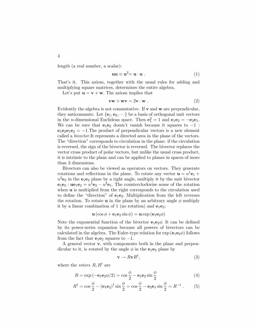
length (a real number, a scalar):

uu ≡ u2= u · u . (1)

That’s it. This axiom, together with the usual rules for adding andmultiplying square matrices, determines the entire algebra.Let’s put u = v +w. The axiom implies that

vw+wv = 2v ·w . (2)

Evidently the algebra is not commutative. If v and w are perpendicular,they anticommute. Let e1, e2, · · · be a basis of orthogonal unit vectorsin the n-dimensional Euclidean space. Then e21 = 1 and e1e2 = −e2e1.We can be sure that e1e2 doesn’t vanish because it squares to −1 :e1e2e1e2 = −1.The product of perpendicular vectors is a new elementcalled a bivector.It represents a directed area in the plane of the vectors.The “direction” corresponds to circulation in the plane: if the circulationis reversed, the sign of the bivector is reversed. The bivector replaces thevector cross product of polar vectors, but unlike the usual cross product,it is intrinsic to the plane and can be applied to planes in spaces of morethan 3 dimensions.Bivectors can also be viewed as operators on vectors. They generate

rotations and reflections in the plane. To rotate any vector u = u1e1 +u2e2 in the e1e2 plane by a right angle, multiply it by the unit bivectore1e2 : ue1e2 = u1e2 − u2e1. The counterclockwise sense of the rotationwhen u is multiplied from the right corresponds to the circulation usedto define the “direction” of e1e2. Multiplication from the left reversesthe rotation. To rotate u in the plane by an arbitrary angle φ multiplyit by a linear combination of 1 (no rotation) and e1e2:

u (cosφ+ e1e2 sinφ) = u exp (e1e2φ)

Note the exponential function of the bivector e1e2φ. It can be definedby its power-series expansion because all powers of bivectors can becalculated in the algebra. The Euler-type relation for exp (e1e2φ) followsfrom the fact that e1e2 squares to −1.A general vector v, with components both in the plane and perpen-

dicular to it, is rotated by the angle φ in the e1e2 plane by

v→ RvR†, (3)

where the rotors R,R† are

R = exp (−e1e2φ/2) = cos φ2− e1e2 sin φ

2(4)

R† = cosφ

2− (e1e2)† sin φ

2= cos

φ

2− e2e1 sin φ

2= R−1 . (5)

Geometry of Paravector Space 5

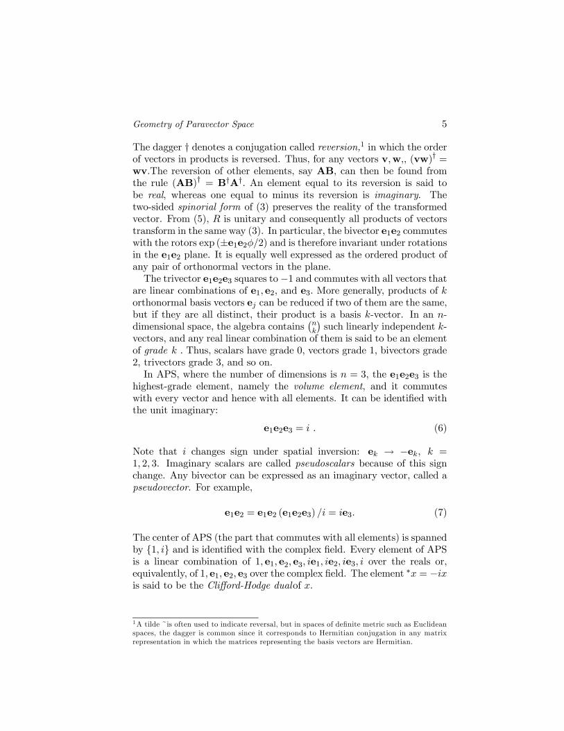
The dagger † denotes a conjugation called reversion,1 in which the orderof vectors in products is reversed. Thus, for any vectors v,w,, (vw)† =wv.The reversion of other elements, say AB, can then be found fromthe rule (AB)† = B†A†. An element equal to its reversion is said tobe real, whereas one equal to minus its reversion is imaginary. Thetwo-sided spinorial form of (3) preserves the reality of the transformedvector. From (5), R is unitary and consequently all products of vectorstransform in the same way (3). In particular, the bivector e1e2 commuteswith the rotors exp (±e1e2φ/2) and is therefore invariant under rotationsin the e1e2 plane. It is equally well expressed as the ordered product ofany pair of orthonormal vectors in the plane.The trivector e1e2e3 squares to−1 and commutes with all vectors that

are linear combinations of e1, e2, and e3. More generally, products of korthonormal basis vectors ej can be reduced if two of them are the same,but if they are all distinct, their product is a basis k-vector. In an n-dimensional space, the algebra contains

¡nk

¢such linearly independent k-

vectors, and any real linear combination of them is said to be an elementof grade k . Thus, scalars have grade 0, vectors grade 1, bivectors grade2, trivectors grade 3, and so on.In APS, where the number of dimensions is n = 3, the e1e2e3 is the

highest-grade element, namely the volume element, and it commuteswith every vector and hence with all elements. It can be identified withthe unit imaginary:

e1e2e3 = i . (6)

Note that i changes sign under spatial inversion: ek → −ek, k =1, 2, 3. Imaginary scalars are called pseudoscalars because of this signchange. Any bivector can be expressed as an imaginary vector, called apseudovector. For example,

e1e2 = e1e2 (e1e2e3) /i = ie3. (7)

The center of APS (the part that commutes with all elements) is spannedby 1, i and is identified with the complex field. Every element of APSis a linear combination of 1, e1, e2, e3, ie1, ie2, ie3, i over the reals or,equivalently, of 1, e1, e2, e3 over the complex field. The element ∗x = −ixis said to be the Clifford-Hodge dualof x.

1A tilde ~is often used to indicate reversal, but in spaces of definite metric such as Euclideanspaces, the dagger is common since it corresponds to Hermitian conjugation in any matrixrepresentation in which the matrices representing the basis vectors are Hermitian.

6

Existence

We should check that our algebra exists. It is possible to define struc-tures that are not self-consistent. The existence of a matrix represen-tation is sufficient to prove existence. The canonical one replaces unitvectors by Pauli spin matrices. There are an infinite number of validrepresentations. They share the same algebra and that is all that mat-ters.

2. Paravector Space as Spacetime

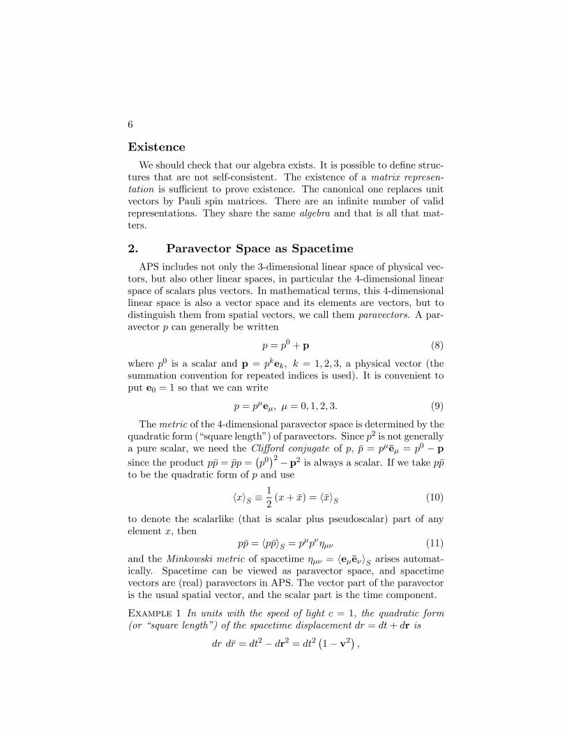
APS includes not only the 3-dimensional linear space of physical vec-tors, but also other linear spaces, in particular the 4-dimensional linearspace of scalars plus vectors. In mathematical terms, this 4-dimensionallinear space is also a vector space and its elements are vectors, but todistinguish them from spatial vectors, we call them paravectors. A par-avector p can generally be written

p = p0 + p (8)

where p0 is a scalar and p = pkek, k = 1, 2, 3, a physical vector (thesummation convention for repeated indices is used). It is convenient toput e0 = 1 so that we can write

p = pµeµ, µ = 0, 1, 2, 3. (9)

Themetric of the 4-dimensional paravector space is determined by thequadratic form (“square length”) of paravectors. Since p2 is not generallya pure scalar, we need the Clifford conjugate of p, p = pµeµ = p0 − psince the product pp = pp =

¡p0¢2 −p2 is always a scalar. If we take pp

to be the quadratic form of p and use

hxiS ≡1

2(x+ x) = hxiS (10)

to denote the scalarlike (that is scalar plus pseudoscalar) part of anyelement x, then

pp = hppiS = pµpνηµν (11)

and the Minkowski metric of spacetime ηµν = heµeνiS arises automat-ically. Spacetime can be viewed as paravector space, and spacetimevectors are (real) paravectors in APS. The vector part of the paravectoris the usual spatial vector, and the scalar part is the time component.

Example 1 In units with the speed of light c = 1, the quadratic form(or “square length”) of the spacetime displacement dr = dt+ dr is

dr dr = dt2 − dr2 = dt2¡1− v2¢ ,

Geometry of Paravector Space 7

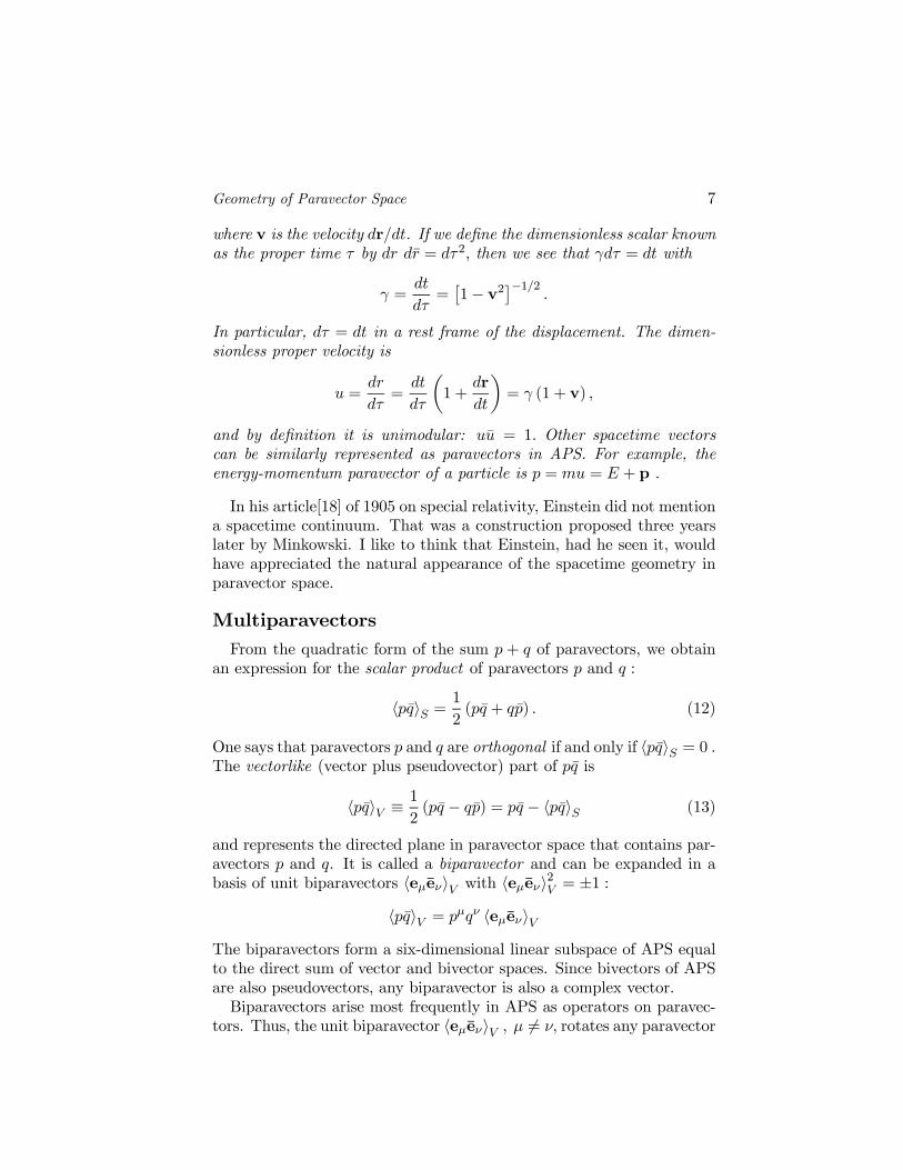
where v is the velocity dr/dt. If we define the dimensionless scalar knownas the proper time τ by dr dr = dτ2, then we see that γdτ = dt with

γ =dt

dτ=£1− v2¤−1/2 .

In particular, dτ = dt in a rest frame of the displacement. The dimen-sionless proper velocity is

u =dr

dτ=

dt

dτ

µ1 +

dr

dt

¶= γ (1 + v) ,

and by definition it is unimodular: uu = 1. Other spacetime vectorscan be similarly represented as paravectors in APS. For example, theenergy-momentum paravector of a particle is p = mu = E + p .

In his article[18] of 1905 on special relativity, Einstein did not mentiona spacetime continuum. That was a construction proposed three yearslater by Minkowski. I like to think that Einstein, had he seen it, wouldhave appreciated the natural appearance of the spacetime geometry inparavector space.

Multiparavectors

From the quadratic form of the sum p + q of paravectors, we obtainan expression for the scalar product of paravectors p and q :

hpqiS =1

2(pq + qp) . (12)

One says that paravectors p and q are orthogonal if and only if hpqiS = 0 .The vectorlike (vector plus pseudovector) part of pq is

hpqiV ≡1

2(pq − qp) = pq − hpqiS (13)

and represents the directed plane in paravector space that contains par-avectors p and q. It is called a biparavector and can be expanded in abasis of unit biparavectors heµeνiV with heµeνi2V = ±1 :

hpqiV = pµqν heµeνiVThe biparavectors form a six-dimensional linear subspace of APS equalto the direct sum of vector and bivector spaces. Since bivectors of APSare also pseudovectors, any biparavector is also a complex vector.Biparavectors arise most frequently in APS as operators on paravec-

tors. Thus, the unit biparavector heµeνiV , µ 6= ν, rotates any paravector

8

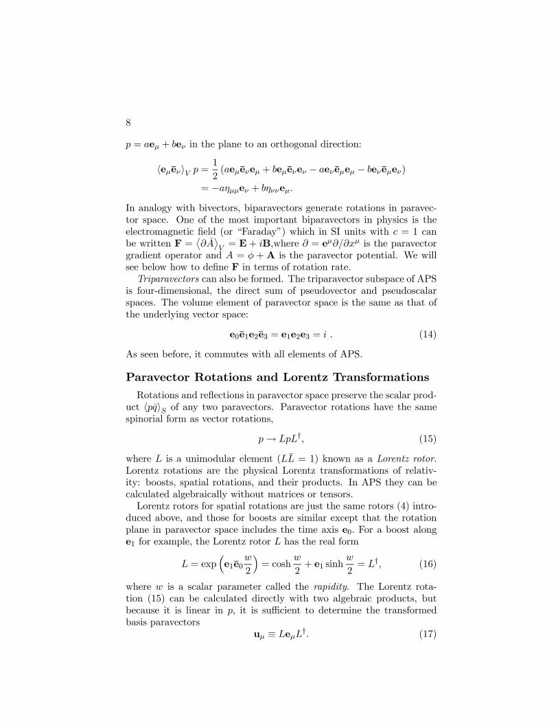
p = aeµ + beν in the plane to an orthogonal direction:

heµeνiV p =1

2(aeµeνeµ + beµeνeν − aeν eµeµ − beν eµeν)

= −aηµµeν + bηννeµ.

In analogy with bivectors, biparavectors generate rotations in paravec-tor space. One of the most important biparavectors in physics is theelectromagnetic field (or “Faraday”) which in SI units with c = 1 canbe written F =

­∂A®V= E+ iB,where ∂ = eµ∂/∂xµ is the paravector

gradient operator and A = φ +A is the paravector potential. We willsee below how to define F in terms of rotation rate.Triparavectors can also be formed. The triparavector subspace of APS

is four-dimensional, the direct sum of pseudovector and pseudoscalarspaces. The volume element of paravector space is the same as that ofthe underlying vector space:

e0e1e2e3 = e1e2e3 = i . (14)

As seen before, it commutes with all elements of APS.

Paravector Rotations and Lorentz Transformations

Rotations and reflections in paravector space preserve the scalar prod-uct hpqiS of any two paravectors. Paravector rotations have the samespinorial form as vector rotations,

p→ LpL†, (15)

where L is a unimodular element (LL = 1) known as a Lorentz rotor.Lorentz rotations are the physical Lorentz transformations of relativ-ity: boosts, spatial rotations, and their products. In APS they can becalculated algebraically without matrices or tensors.Lorentz rotors for spatial rotations are just the same rotors (4) intro-

duced above, and those for boosts are similar except that the rotationplane in paravector space includes the time axis e0. For a boost alonge1 for example, the Lorentz rotor L has the real form

L = exp³e1e0

w

2

´= cosh

w

2+ e1 sinh

w

2= L†, (16)

where w is a scalar parameter called the rapidity. The Lorentz rota-tion (15) can be calculated directly with two algebraic products, butbecause it is linear in p, it is sufficient to determine the transformedbasis paravectors

uµ ≡ LeµL†. (17)

Geometry of Paravector Space 9

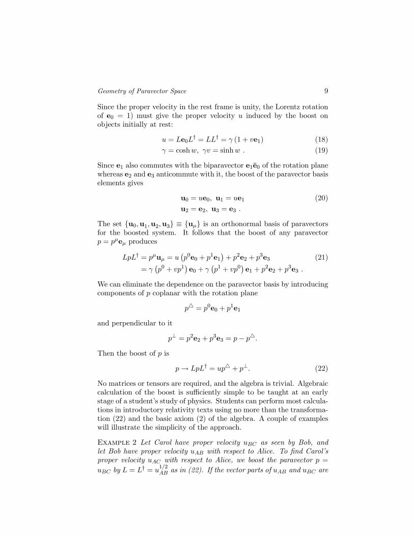
Since the proper velocity in the rest frame is unity, the Lorentz rotationof e0 = 1) must give the proper velocity u induced by the boost onobjects initially at rest:

u = Le0L† = LL† = γ (1 + ve1) (18)

γ = coshw, γv = sinhw . (19)

Since e1 also commutes with the biparavector e1e0 of the rotation planewhereas e2 and e3 anticommute with it, the boost of the paravector basiselements gives

u0 = ue0, u1 = ue1 (20)

u2 = e2, u3 = e3 .

The set u0,u1,u2,u3 ≡ uµ is an orthonormal basis of paravectorsfor the boosted system. It follows that the boost of any paravectorp = pµeµ produces

LpL† = pµuµ = u¡p0e0 + p1e1

¢+ p2e2 + p3e3 (21)

= γ¡p0 + vp1

¢e0 + γ

¡p1 + vp0

¢e1 + p2e2 + p3e3 .

We can eliminate the dependence on the paravector basis by introducingcomponents of p coplanar with the rotation plane

p4 = p0e0 + p1e1

and perpendicular to it

p⊥ = p2e2 + p3e3 = p− p4.

Then the boost of p is

p→ LpL† = up4 + p⊥. (22)

No matrices or tensors are required, and the algebra is trivial. Algebraiccalculation of the boost is sufficiently simple to be taught at an earlystage of a student’s study of physics. Students can perform most calcula-tions in introductory relativity texts using no more than the transforma-tion (22) and the basic axiom (2) of the algebra. A couple of exampleswill illustrate the simplicity of the approach.

Example 2 Let Carol have proper velocity uBC as seen by Bob, andlet Bob have proper velocity uAB with respect to Alice. To find Carol’sproper velocity uAC with respect to Alice, we boost the paravector p =uBC by L = L† = u

1/2AB as in (22). If the vector parts of uAB and uBC are

10

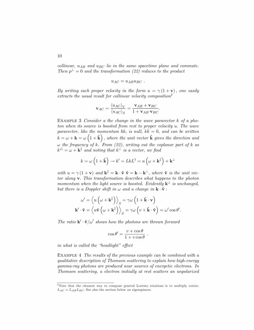
collinear, uAB and uBC lie in the same spacetime plane and commute.Then p⊥ = 0 and the transformation (22) reduces to the product

uAC = uABuBC .

By writing each proper velocity in the form u = γ (1 + v) , one easilyextracts the usual result for collinear velocity composition2

vAC =huACiVhuACiS

=vAB + vBC1 + vAB·vBC .

Example 3 Consider a the change in the wave paravector k of a pho-ton when its source is boosted from rest to proper velocity u. The waveparavector, like the momentum ~k, is null, kk = 0, and can be writtenk = ω + k = ω

³1 + k

´, where the unit vector k gives the direction and

ω the frequency of k. From (22), writing out the coplanar part of k ask4 = ω + kk and noting that k⊥ is a vector, we find

k = ω³1 + k

´→ k0 = LkL† = u

³ω + kk

´+ k⊥

with u = γ (1 + v) and kk = k · v v = k− k⊥, where v is the unit vec-tor along v. This transformation describes what happens to the photonmomentum when the light source is boosted. Evidently k⊥ is unchanged,but there is a Doppler shift in ω and a change in k · v :

ω0 =Du³ω + kk

´ES= γω

³1 + k · v

´k0 · v =

Duv³ω + kk

´ES= γω

³v + k · v

´= ω0 cos θ0.

The ratio k0 · v/ω0 shows how the photons are thrown forward

cos θ0 =v + cos θ

1 + v cos θ.

in what is called the “headlight” effect

Example 4 The results of the previous example can be combined with aqualitative description of Thomson scattering to explain how high-energygamma-ray photons are produced near sources of energetic electrons. InThomson scattering, a electron initially at rest scatters an unpolarized

2Note that the cleanest way to compose general Lorentz rotations is to multiply rotors:LAC = LABLBC . See also the section below on eigenspinors.

Geometry of Paravector Space 11

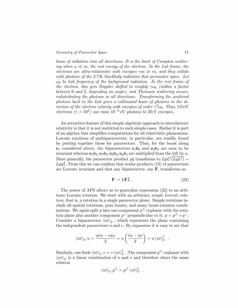
beam of radiation into all directions. It is the limit of Compton scatter-ing when ω ¿ m, the rest energy of the electron. In the Lab frame, theelectrons are ultra-relativistic with energies γm À m, and they collidewith photons of the 2.7K blackbody radiation that permeates space. Letω0 be Lab frequency of the background radiation. In the rest frame ofthe electron, this gets Doppler shifted to roughly γω0 (within a factorbetween 0 and 2, depending on angle), and Thomson scattering occurs,redistributing the photons in all directions. Transforming the scatteredphotons back to the Lab gives a collimated beam of photons in the di-rection of the electron velocity with energies of order γ2ω0. Thus, 5GeVelectrons (γ = 104) can raise 10−2 eV photons to MeV energies.

An attractive feature of this simple algebraic approach to introductoryrelativity is that it is not restricted to such simple cases. Rather it is partof an algebra that simplifies computations for all relativistic phenomena.Lorentz rotations of multiparavectors, in particular, are readily foundby putting together those for paravectors. Thus, for the boost alonge1 considered above, the biparavectors e1e0 and e2e3 are seen to beinvariant whereas e1e2, e1e3, e0e2, e0e3 are multiplied from the left by u.More generally, the paravector product pq transforms to LpL†(LqL†) =LpqL. From this we can confirm that scalar products (12) of paravectorsare Lorentz invariant and that any biparavector, say F, transforms as

F→ LFL . (23)

The power of APS allows us to generalize expression (22) to an arbi-trary Lorentz rotation. We start with an arbitrary simple Lorentz rota-tion, that is, a rotation in a single paravector plane. Simple rotations in-clude all spatial rotations, pure boosts, and many boost-rotation combi-nations. We again split p into one component p4 coplanar with the rota-tion plane plus another component p⊥ perpendicular to it: p = p4+p⊥.Consider a biparavector huviV , which represents the plane containingthe independent paravectors u and v. By expansion it is easy to see that

huviV u =uvu− vuu

2= u

µvu− uv

2

¶= u huvi†V .

Similarly, one finds huviV v = v huvi†V .The component p4 coplanar withhuviV is a linear combination of u and v and therefore obeys the samerelation

huviV p4 = p4 huvi†V .

12

On the other hand, the component p⊥ is orthogonal to u and v,­up⊥

®S=

0 =­up⊥

®Sand similarly for u replaced by v. Consequently,

huviV p⊥ =uvp⊥ − vup⊥

2= −p⊥ huvi†V .

It follows that if L is any Lorentz rotation in the huviV plane, then

p4L† = Lp4, p⊥L† = Lp⊥,

and the rotation (15) reduces to

p→ Lp4L† + Lp⊥L† = L2p4 + p⊥. (24)

Expression (22) is a special case of this relation for a pure boost. We cannow generalize the result further to include compound Lorentz rotations.Any rotor can be expressed as

L = ± expµ1

2W

¶, (25)

and the arbitrary biparavectorW can always be expanded as a sum ofsimple biparavectors W =W1 +W2 = (1 + iα)W1, where α is a realscalar. The relation W2 = iαW1 means that W2 is proportional tothe dual ofW1 so thatW1 andW2 represent orthogonal planes: everyparavector in W1 is orthogonal to every paravector in W2. Since W1

andW2 commute, L can be written as a product of commuting simpleLorentz rotations:

L = L1L2, L1 = eW1/2, L2 = eW2/2.

Every paravector p can be split into one component, p1, coplanar withW1 and another, p2, coplanar withW2 . Two applications of the simpletransformation result (24) gives its generalization

p→ LpL† = L1L2 (p1 + p2)L†2L

†1 = L21p1 + L22p2 . (26)

Note that the Lorentz transformations of paravectors p and p† are thesame, as are those of biparavectors F and F. However, p and p havedistinct transformations as do F and F†. As a consequence, Lorentztransformations mix time and space components of p, but not its real andimaginary parts, whereas such transformations of F leave F vectorlikebut mix vector (real) and bivector (imaginary) parts.

Geometry of Paravector Space 13

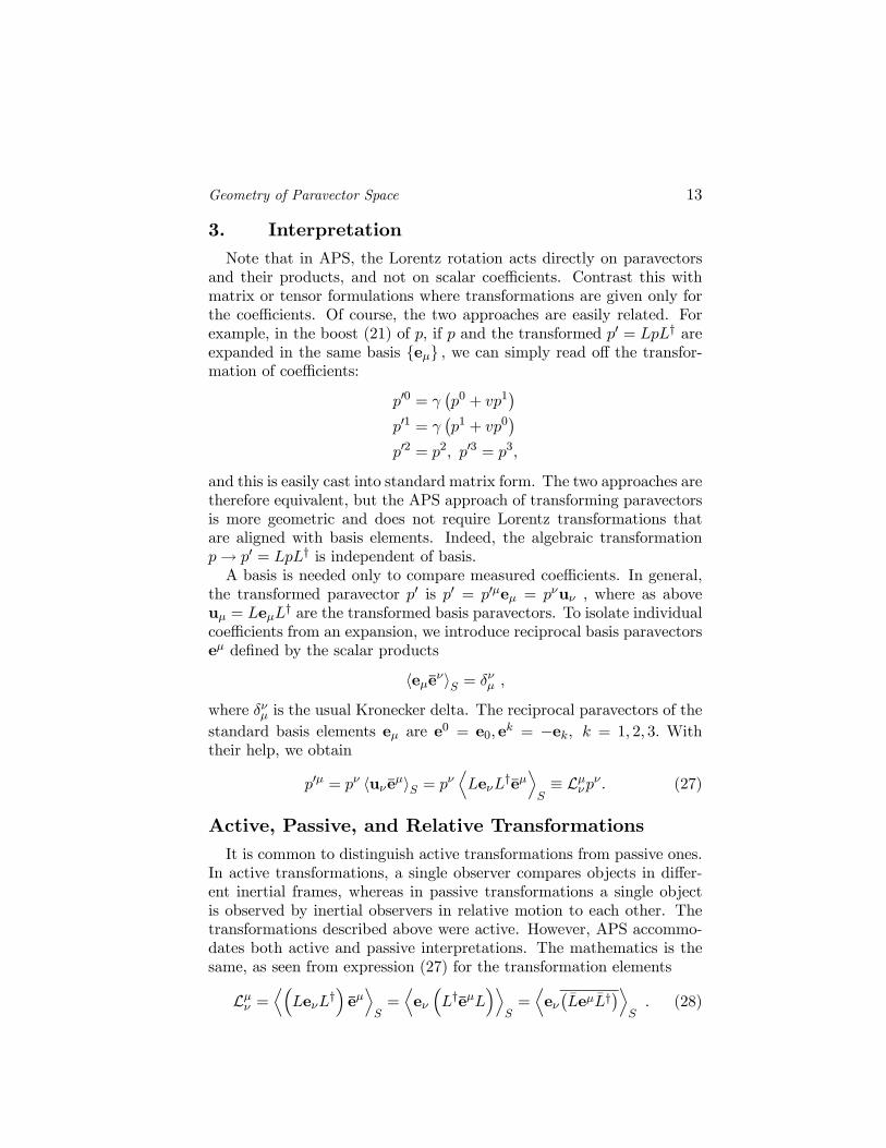
3. Interpretation

Note that in APS, the Lorentz rotation acts directly on paravectorsand their products, and not on scalar coefficients. Contrast this withmatrix or tensor formulations where transformations are given only forthe coefficients. Of course, the two approaches are easily related. Forexample, in the boost (21) of p, if p and the transformed p0 = LpL† areexpanded in the same basis eµ , we can simply read off the transfor-mation of coefficients:

p00 = γ¡p0 + vp1

¢p01 = γ

¡p1 + vp0

¢p02 = p2, p03 = p3,

and this is easily cast into standard matrix form. The two approaches aretherefore equivalent, but the APS approach of transforming paravectorsis more geometric and does not require Lorentz transformations thatare aligned with basis elements. Indeed, the algebraic transformationp→ p0 = LpL† is independent of basis.A basis is needed only to compare measured coefficients. In general,

the transformed paravector p0 is p0 = p0µeµ = pνuν , where as aboveuµ = LeµL

† are the transformed basis paravectors. To isolate individualcoefficients from an expansion, we introduce reciprocal basis paravectorseµ defined by the scalar products

heµeνiS = δνµ ,

where δνµ is the usual Kronecker delta. The reciprocal paravectors of thestandard basis elements eµ are e0 = e0, e

k = −ek, k = 1, 2, 3. Withtheir help, we obtain

p0µ = pν huν eµiS = pνDLeνL

†eµES≡ Lµνpν . (27)

Active, Passive, and Relative Transformations

It is common to distinguish active transformations from passive ones.In active transformations, a single observer compares objects in differ-ent inertial frames, whereas in passive transformations a single objectis observed by inertial observers in relative motion to each other. Thetransformations described above were active. However, APS accommo-dates both active and passive interpretations. The mathematics is thesame, as seen from expression (27) for the transformation elements

Lµν =D³

LeνL†´eµES=Deν

³L†eµL

´ES=Deν¡LeµL†

¢ES. (28)

14

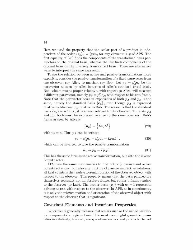
Here we used the property that the scalar part of a product is inde-pendent of the order hxyiS = hyxiS for any elements x, y of APS. Thefirst equality of (28) finds the components of the transformed basis par-avectors on the original basis, whereas the last finds components of theoriginal basis on the inversely transformed basis. These are alternativeways to interpret the same expression.To see the relation between active and passive transformations more

explicitly, consider the passive transformation of a fixed paravector fromone observer, say Alice, to another, say Bob. Let pA = pµAeµ be theparavector as seen by Alice in terms of Alice’s standard (rest) basis.Bob, who moves at proper velocity u with respect to Alice, will measurea different paravector, namely pB = pµBeµ, with respect to his rest frame.Note that the paravector basis in expansions of both pA and pB is thesame, namely the standard basis eµ , even though pA is expressedrelative to Alice and pB relative to Bob. The reason is that the standardbasis eµ is relative; it is at rest relative to the observer. To relate pAand pB, both must be expressed relative to the same observer. Bob’sframe as seen by Alice is

uµ =nLeµL

†o

(29)

with u0 = u. Thus pA can be written

pA = pµAeµ = pνBuν = LpBL† , (30)

which can be inverted to give the passive transformation

pA → pB = LpAL†. (31)

This has the same form as the active transformation, but with the inverseLorentz rotor.APS uses the same mathematics to find not only passive and active

Lorentz rotations, but also any mixture of passive and active rotations:all that counts is the relative Lorentz rotation of the observed object withrespect to the observer. This property means that the basis paravectorsthemselves represent not an absolute frame, but rather a frame relativeto the observer (or Lab). The proper basis eµ with e0 = 1 representsa frame at rest with respect to the observer. In APS, as in experiments,it is only the relative motion and orientation of the observed object withrespect to the observer that is significant.

Covariant Elements and Invariant Properties

Experiments generally measure real scalars such as the size of paravec-tor components on a given basis. The most meaningful geometric quan-tities in relativity, however, are spacetime vectors and products thereof

Geometry of Paravector Space 15

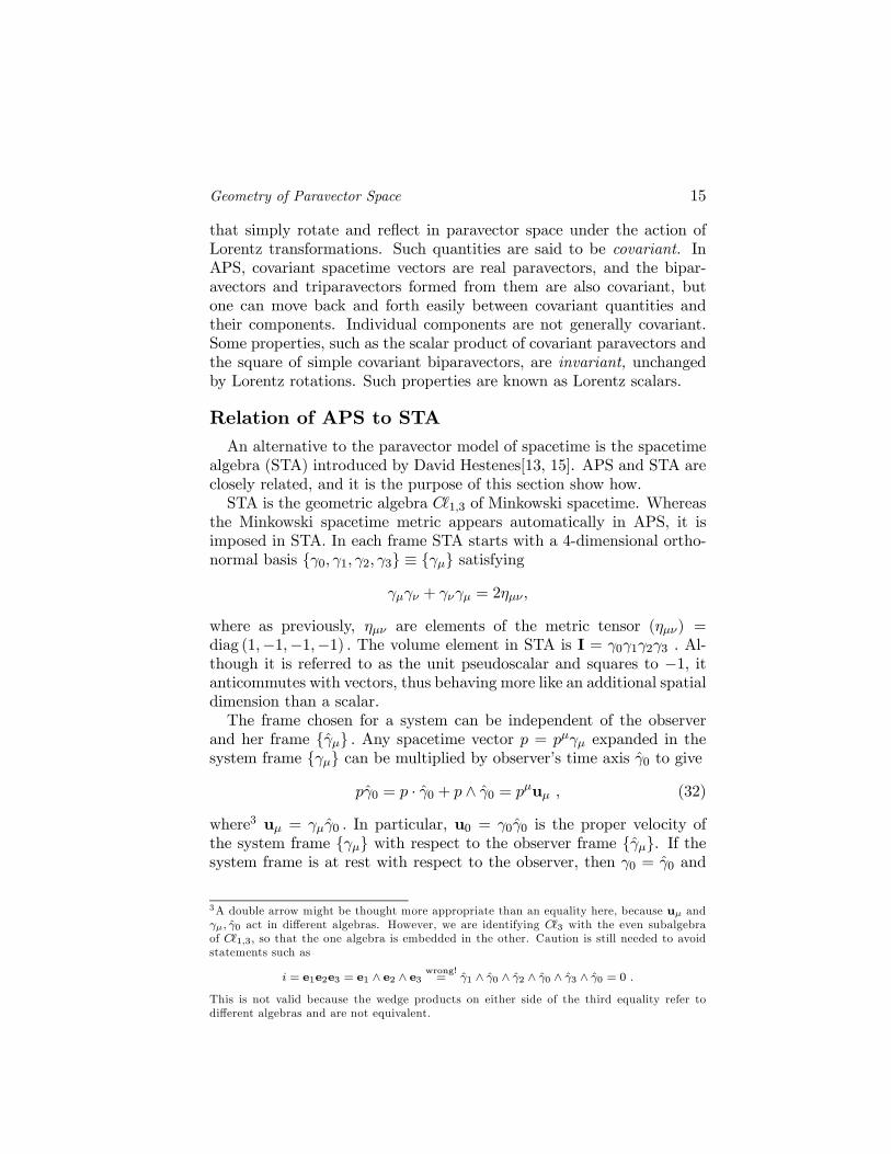
that simply rotate and reflect in paravector space under the action ofLorentz transformations. Such quantities are said to be covariant. InAPS, covariant spacetime vectors are real paravectors, and the bipar-avectors and triparavectors formed from them are also covariant, butone can move back and forth easily between covariant quantities andtheir components. Individual components are not generally covariant.Some properties, such as the scalar product of covariant paravectors andthe square of simple covariant biparavectors, are invariant, unchangedby Lorentz rotations. Such properties are known as Lorentz scalars.

Relation of APS to STA

An alternative to the paravector model of spacetime is the spacetimealgebra (STA) introduced by David Hestenes[13, 15]. APS and STA areclosely related, and it is the purpose of this section show how.STA is the geometric algebra C 1,3 of Minkowski spacetime. Whereas

the Minkowski spacetime metric appears automatically in APS, it isimposed in STA. In each frame STA starts with a 4-dimensional ortho-normal basis γ0, γ1, γ2, γ3 ≡ γµ satisfying

γµγν + γνγµ = 2ηµν ,

where as previously, ηµν are elements of the metric tensor (ηµν) =diag (1,−1,−1,−1) . The volume element in STA is I = γ0γ1γ2γ3 . Al-though it is referred to as the unit pseudoscalar and squares to −1, itanticommutes with vectors, thus behaving more like an additional spatialdimension than a scalar.The frame chosen for a system can be independent of the observer

and her frame γµ . Any spacetime vector p = pµγµ expanded in thesystem frame γµ can be multiplied by observer’s time axis γ0 to give

pγ0 = p · γ0 + p ∧ γ0 = pµuµ , (32)

where3 uµ = γµγ0 . In particular, u0 = γ0γ0 is the proper velocity ofthe system frame γµ with respect to the observer frame γµ. If thesystem frame is at rest with respect to the observer, then γ0 = γ0 and

3A double arrow might be thought more appropriate than an equality here, because uµ andγµ, γ0 act in different algebras. However, we are identifying C 3 with the even subalgebraof C 1,3, so that the one algebra is embedded in the other. Caution is still needed to avoidstatements such as

i = e1e2e3 = e1 ∧ e2 ∧ e3 wrong!= γ1 ∧ γ0 ∧ γ2 ∧ γ0 ∧ γ3 ∧ γ0 = 0 .

This is not valid because the wedge products on either side of the third equality refer todifferent algebras and are not equivalent.

16

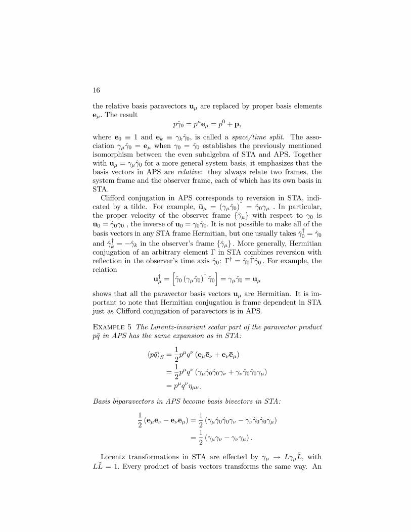
the relative basis paravectors uµ are replaced by proper basis elementseµ. The result

pγ0 = pµeµ = p0 + p,

where e0 ≡ 1 and ek ≡ γkγ0, is called a space/time split. The asso-ciation γµγ0 = eµ when γ0 = γ0 establishes the previously mentionedisomorphism between the even subalgebra of STA and APS. Togetherwith uµ = γµγ0 for a more general system basis, it emphasizes that thebasis vectors in APS are relative: they always relate two frames, thesystem frame and the observer frame, each of which has its own basis inSTA.Clifford conjugation in APS corresponds to reversion in STA, indi-

cated by a tilde. For example, uµ = (γµγ0)˜ = γ0γµ . In particular,

the proper velocity of the observer frame γµ with respect to γ0 isu0 = γ0γ0 , the inverse of u0 = γ0γ0. It is not possible to make all of thebasis vectors in any STA frame Hermitian, but one usually takes γ†0 = γ0and γ†k = −γk in the observer’s frame γµ . More generally, Hermitianconjugation of an arbitrary element Γ in STA combines reversion withreflection in the observer’s time axis γ0: Γ† = γ0Γγ0 . For example, therelation

u†µ =hγ0 (γµγ0)

˜ γ0

i= γµγ0 = uµ

shows that all the paravector basis vectors uµ are Hermitian. It is im-portant to note that Hermitian conjugation is frame dependent in STAjust as Clifford conjugation of paravectors is in APS.

Example 5 The Lorentz-invariant scalar part of the paravector productpq in APS has the same expansion as in STA:

hpqiS =1

2pµqν (eµeν + eν eµ)

=1

2pµqν (γµγ0γ0γν + γν γ0γ0γµ)

= pµqνηµν .

Basis biparavectors in APS become basis bivectors in STA:

1

2(eµeν − eν eµ) = 1

2(γµγ0γ0γν − γν γ0γ0γµ)

=1

2(γµγν − γνγµ) .

Lorentz transformations in STA are effected by γµ → LγµL, withLL = 1. Every product of basis vectors transforms the same way. An

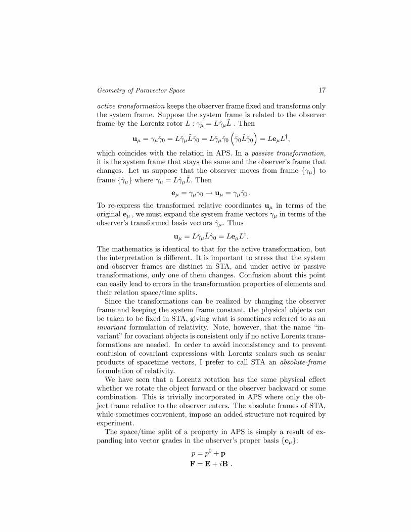
Geometry of Paravector Space 17

active transformation keeps the observer frame fixed and transforms onlythe system frame. Suppose the system frame is related to the observerframe by the Lorentz rotor L : γµ = LγµL . Then

uµ = γµγ0 = LγµLγ0 = Lγµγ0

³γ0Lγ0

´= LeµL

†,

which coincides with the relation in APS. In a passive transformation,it is the system frame that stays the same and the observer’s frame thatchanges. Let us suppose that the observer moves from frame γµ toframe γµ where γµ = LγµL. Then

eµ = γµγ0 → uµ = γµγ0 .

To re-express the transformed relative coordinates uµ in terms of theoriginal eµ , we must expand the system frame vectors γµ in terms of theobserver’s transformed basis vectors γµ. Thus

uµ = LγµLγ0 = LeµL†.

The mathematics is identical to that for the active transformation, butthe interpretation is different. It is important to stress that the systemand observer frames are distinct in STA, and under active or passivetransformations, only one of them changes. Confusion about this pointcan easily lead to errors in the transformation properties of elements andtheir relation space/time splits.Since the transformations can be realized by changing the observer

frame and keeping the system frame constant, the physical objects canbe taken to be fixed in STA, giving what is sometimes referred to as aninvariant formulation of relativity. Note, however, that the name “in-variant” for covariant objects is consistent only if no active Lorentz trans-formations are needed. In order to avoid inconsistency and to preventconfusion of covariant expressions with Lorentz scalars such as scalarproducts of spacetime vectors, I prefer to call STA an absolute-frameformulation of relativity.We have seen that a Lorentz rotation has the same physical effect

whether we rotate the object forward or the observer backward or somecombination. This is trivially incorporated in APS where only the ob-ject frame relative to the observer enters. The absolute frames of STA,while sometimes convenient, impose an added structure not required byexperiment.The space/time split of a property in APS is simply a result of ex-

panding into vector grades in the observer’s proper basis eµ:p = p0 + p

F = E+ iB .

18

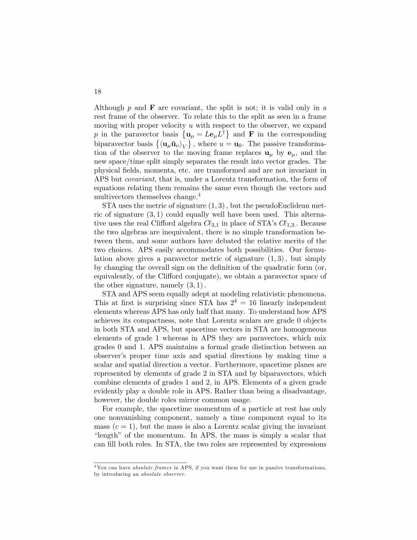
Although p and F are covariant, the split is not; it is valid only in arest frame of the observer. To relate this to the split as seen in a framemoving with proper velocity u with respect to the observer, we expandp in the paravector basis

©uµ = LeµL

†ª and F in the correspondingbiparavector basis

©huµuνiV ª , where u = u0. The passive transforma-tion of the observer to the moving frame replaces uµ by eµ, and thenew space/time split simply separates the result into vector grades. Thephysical fields, momenta, etc. are transformed and are not invariant inAPS but covariant, that is, under a Lorentz transformation, the form ofequations relating them remains the same even though the vectors andmultivectors themselves change.4

STA uses the metric of signature (1, 3) , but the pseudoEuclidean met-ric of signature (3, 1) could equally well have been used. This alterna-tive uses the real Clifford algebra C 3,1 in place of STA’s C 1,3.. Becausethe two algebras are inequivalent, there is no simple transformation be-tween them, and some authors have debated the relative merits of thetwo choices. APS easily accommodates both possibilities. Our formu-lation above gives a paravector metric of signature (1, 3) , but simplyby changing the overall sign on the definition of the quadratic form (or,equivalently, of the Clifford conjugate), we obtain a paravector space ofthe other signature, namely (3, 1) .STA and APS seem equally adept at modeling relativistic phenomena.

This at first is surprising since STA has 24 = 16 linearly independentelements whereas APS has only half that many. To understand how APSachieves its compactness, note that Lorentz scalars are grade 0 objectsin both STA and APS, but spacetime vectors in STA are homogeneouselements of grade 1 whereas in APS they are paravectors, which mixgrades 0 and 1. APS maintains a formal grade distinction between anobserver’s proper time axis and spatial directions by making time ascalar and spatial direction a vector. Furthermore, spacetime planes arerepresented by elements of grade 2 in STA and by biparavectors, whichcombine elements of grades 1 and 2, in APS. Elements of a given gradeevidently play a double role in APS. Rather than being a disadvantage,however, the double roles mirror common usage.For example, the spacetime momentum of a particle at rest has only

one nonvanishing component, namely a time component equal to itsmass (c = 1), but the mass is also a Lorentz scalar giving the invariant“length” of the momentum. In APS, the mass is simply a scalar thatcan fill both roles. In STA, the two roles are represented by expressions

4You can have absolute frames in APS, if you want them for use in passive transformations,by introducing an absolute observer.

Geometry of Paravector Space 19

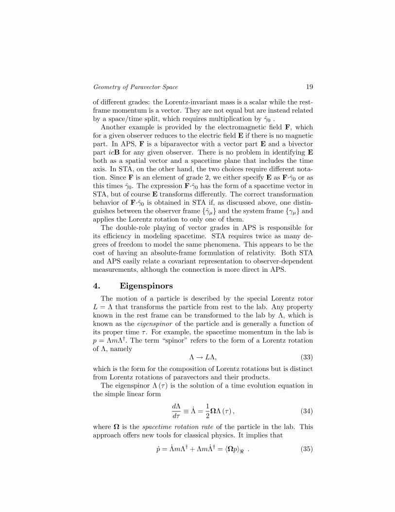
of different grades: the Lorentz-invariant mass is a scalar while the rest-frame momentum is a vector. They are not equal but are instead relatedby a space/time split, which requires multiplication by γ0 .Another example is provided by the electromagnetic field F, which

for a given observer reduces to the electric field E if there is no magneticpart. In APS, F is a biparavector with a vector part E and a bivectorpart icB for any given observer. There is no problem in identifying Eboth as a spatial vector and a spacetime plane that includes the timeaxis. In STA, on the other hand, the two choices require different nota-tion. Since F is an element of grade 2, we either specify E as F·γ0 or asthis times γ0. The expression F·γ0 has the form of a spacetime vector inSTA, but of course E transforms differently. The correct transformationbehavior of F·γ0 is obtained in STA if, as discussed above, one distin-guishes between the observer frame γµ and the system frame γµ andapplies the Lorentz rotation to only one of them.The double-role playing of vector grades in APS is responsible for

its efficiency in modeling spacetime. STA requires twice as many de-grees of freedom to model the same phenomena. This appears to be thecost of having an absolute-frame formulation of relativity. Both STAand APS easily relate a covariant representation to observer-dependentmeasurements, although the connection is more direct in APS.

4. Eigenspinors

The motion of a particle is described by the special Lorentz rotorL = Λ that transforms the particle from rest to the lab. Any propertyknown in the rest frame can be transformed to the lab by Λ, which isknown as the eigenspinor of the particle and is generally a function ofits proper time τ . For example, the spacetime momentum in the lab isp = ΛmΛ†. The term “spinor” refers to the form of a Lorentz rotationof Λ, namely

Λ→ LΛ, (33)

which is the form for the composition of Lorentz rotations but is distinctfrom Lorentz rotations of paravectors and their products.The eigenspinor Λ (τ) is the solution of a time evolution equation in

the simple linear form

dΛ

dτ≡ Λ = 1

2ΩΛ (τ) , (34)

where Ω is the spacetime rotation rate of the particle in the lab. Thisapproach offers new tools for classical physics. It implies that

p = ΛmΛ† + ΛmΛ† = hΩpi< . (35)

20

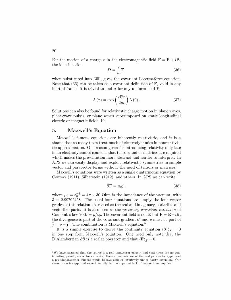
For the motion of a charge e in the electromagnetic field F = E + iB,the identification

Ω =e

mF, (36)

when substituted into (35), gives the covariant Lorentz-force equation.Note that (36) can be taken as a covariant definition of F, valid in anyinertial frame. It is trivial to find Λ for any uniform field F:

Λ (τ) = exp

µeFτ

2m

¶Λ (0) . (37)

Solutions can also be found for relativistic charge motion in plane waves,plane-wave pulses, or plane waves superimposed on static longitudinalelectric or magnetic fields.[19]

5. Maxwell’s Equation

Maxwell’s famous equations are inherently relativistic, and it is ashame that so many texts treat much of electrodynamics in nonrelativis-tic approximation. One reason given for introducing relativity only latein an electrodynamics course is that tensors and or matrices are requiredwhich makes the presentation more abstract and harder to interpret. InAPS we can easily display and exploit relativistic symmetries in simplevector and paravector terms without the need of tensors or matrices.Maxwell’s equations were written as a single quaternionic equation by

Conway (1911), Silberstein (1912), and others. In APS we can write

∂F = µ0j , (38)

where µ0 = ε−10 = 4π × 30 Ohm is the impedance of the vacuum, with3 ≡ 2.99792458. The usual four equations are simply the four vectorgrades of this relation, extracted as the real and imaginary, scalarlike andvectorlike parts. It is also seen as the necessary covariant extension ofCoulomb’s law ∇·E = ρ/ε0. The covariant field is not E but F = E+iB,the divergence is part of the covariant gradient ∂, and ρ must be part ofj = ρ− j . The combination is Maxwell’s equation.5It is a simple exercise to derive the continuity equation h∂jiS = 0

in one step from Maxwell’s equation. One need only note that theD’Alembertian ∂∂ is a scalar operator and that hFiS = 0.

5We have assumed that the source is a real paravector current and that there are no con-tributing pseudoparavector currents. Known currents are of the real paravector type, anda pseudoparavector current would behave counter-intuitively under parity inversion. Ourassumption is supported experimentally by the apparent lack of magnetic monopoles.

Geometry of Paravector Space 21

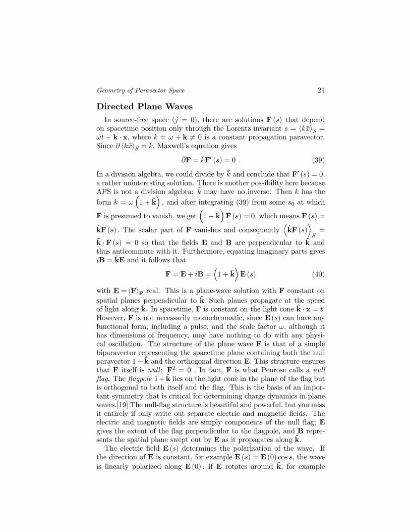
Directed Plane Waves

In source-free space (j = 0), there are solutions F (s) that dependon spacetime position only through the Lorentz invariant s = hkxiS =ωt − k · x, where k = ω + k 6= 0 is a constant propagation paravector.Since ∂ hkxiS = k, Maxwell’s equation gives

∂F = kF0 (s) = 0 . (39)

In a division algebra, we could divide by k and conclude that F0 (s) = 0,a rather uninteresting solution. There is another possibility here becauseAPS is not a division algebra: k may have no inverse. Then k has theform k = ω

³1 + k

´, and after integrating (39) from some s0 at which

F is presumed to vanish, we get³1− k

´F (s) = 0, which means F (s) =

kF (s) . The scalar part of F vanishes and consequentlyDkF (s)

ES=

k · F (s) = 0 so that the fields E and B are perpendicular to k andthus anticommute with it. Furthermore, equating imaginary parts givesiB = kE and it follows that

F = E+ iB =³1 + k

´E (s) (40)

with E = hFi< real. This is a plane-wave solution with F constant onspatial planes perpendicular to k. Such planes propagate at the speedof light along k. In spacetime, F is constant on the light cone k · x = t.However, F is not necessarily monochromatic, since E (s) can have anyfunctional form, including a pulse, and the scale factor ω, although ithas dimensions of frequency, may have nothing to do with any physi-cal oscillation. The structure of the plane wave F is that of a simplebiparavector representing the spacetime plane containing both the nullparavector 1+ k and the orthogonal direction E. This structure ensuresthat F itself is null : F2 = 0 . In fact, F is what Penrose calls a nullflag. The flagpole 1+ k lies on the light cone in the plane of the flag butis orthogonal to both itself and the flag. This is the basis of an impor-tant symmetry that is critical for determining charge dynamics in planewaves.[19] The null-flag structure is beautiful and powerful, but you missit entirely if only write out separate electric and magnetic fields. Theelectric and magnetic fields are simply components of the null flag; Egives the extent of the flag perpendicular to the flagpole, and B repre-sents the spatial plane swept out by E as it propagates along k.The electric field E (s) determines the polarization of the wave. If

the direction of E is constant, for example E (s) = E (0) cos s, the waveis linearly polarized along E (0) . If E rotates around k, for example

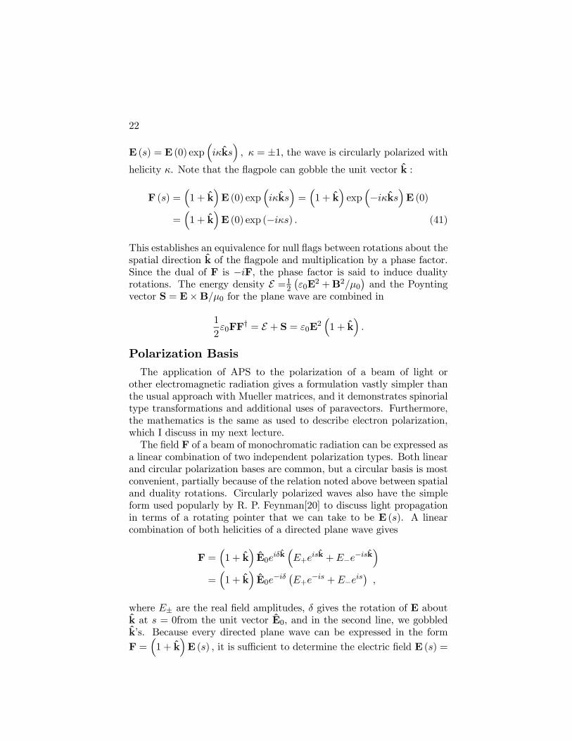
22

E (s) = E (0) exp³iκks

´, κ = ±1, the wave is circularly polarized with

helicity κ. Note that the flagpole can gobble the unit vector k :

F (s) =³1 + k

´E (0) exp

³iκks

´=³1 + k

´exp

³−iκks

´E (0)

=³1 + k

´E (0) exp (−iκs) . (41)

This establishes an equivalence for null flags between rotations about thespatial direction k of the flagpole and multiplication by a phase factor.Since the dual of F is −iF, the phase factor is said to induce dualityrotations. The energy density E =1

2

¡ε0E

2 +B2/µ0¢and the Poynting

vector S = E×B/µ0 for the plane wave are combined in

1

2ε0FF

† = E + S = ε0E2³1 + k

´.

Polarization Basis

The application of APS to the polarization of a beam of light orother electromagnetic radiation gives a formulation vastly simpler thanthe usual approach with Mueller matrices, and it demonstrates spinorialtype transformations and additional uses of paravectors. Furthermore,the mathematics is the same as used to describe electron polarization,which I discuss in my next lecture.The field F of a beam of monochromatic radiation can be expressed as

a linear combination of two independent polarization types. Both linearand circular polarization bases are common, but a circular basis is mostconvenient, partially because of the relation noted above between spatialand duality rotations. Circularly polarized waves also have the simpleform used popularly by R. P. Feynman[20] to discuss light propagationin terms of a rotating pointer that we can take to be E (s). A linearcombination of both helicities of a directed plane wave gives

F =³1 + k

´E0e

iδk³E+e

isk +E−e−isk´

=³1 + k

´E0e

−iδ ¡E+e−is +E−eis¢,

where E± are the real field amplitudes, δ gives the rotation of E aboutk at s = 0from the unit vector E0, and in the second line, we gobbledk’s. Because every directed plane wave can be expressed in the formF =

³1 + k

´E (s) , it is sufficient to determine the electric field E (s) =

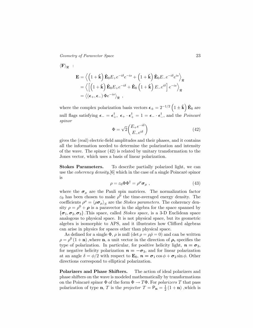
Geometry of Paravector Space 23

hFi< :

E =D³1 + k

´E0E+e

−iδe−is +³1 + k

´E0E−e−iδeis

E<

=Dh³

1 + k´E0E+e

−iδ + E0³1 + k

´E−eiδ

ie−is

E<

=­(²+, ²−)Φe−is

®< ,

where the complex polarization basis vectors ²± = 2−1/2³1± k

´E0 are

null flags satisfying ²− = ²†+, ²+ · ²†+ = 1 = ²− · ²†−, and the Poincaréspinor

Φ =√2

µE+e

−iδ

E−eiδ

¶(42)

gives the (real) electric-field amplitudes and their phases, and it containsall the information needed to determine the polarization and intensityof the wave. The spinor (42) is related by unitary transformation to theJones vector, which uses a basis of linear polarization.

Stokes Parameters. To describe partially polarized light, we canuse the coherency density,[6] which in the case of a single Poincaré spinoris

ρ = ε0ΦΦ† = ρµσµ , (43)

where the σµ are the Pauli spin matrices. The normalization factorε0 has been chosen to make ρ0 the time-averaged energy density. Thecoefficients ρµ = hρσµiS are the Stokes parameters. The coherency den-sity ρ = ρ0 + ρ is a paravector in the algebra for the space spanned byσ1,σ2,σ3 .This space, called Stokes space, is a 3-D Euclidean spaceanalogous to physical space. It is not physical space, but its geometricalgebra is isomorphic to APS, and it illustrates how Clifford algebrascan arise in physics for spaces other than physical space.As defined for a single Φ, ρ is null (det ρ = ρρ = 0) and can be written

ρ = ρ0 (1 + n) ,where n, a unit vector in the direction of ρ, specifies thetype of polarization. In particular, for positive helicity light, n = σ3,for negative helicity polarization n = −σ3, and for linear polarizationat an angle δ = φ/2 with respect to E0, n = σ1 cosφ+ σ2 sinφ. Otherdirections correspond to elliptical polarization.

Polarizers and Phase Shifters. The action of ideal polarizers andphase shifters on the wave is modeled mathematically by transformationson the Poincaré spinor Φ of the form Φ→ TΦ. For polarizers T that passpolarization of type n, T is the projector T = Pn =

12 (1 + n) ,which is

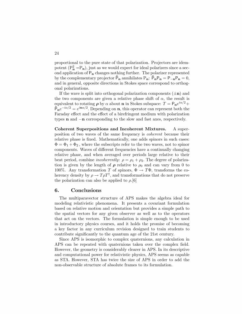
24

proportional to the pure state of that polarization. Projectors are idem-potent (P2n =Pn), just as we would expect for ideal polarizers since a sec-ond application of Pn changes nothing further. The polarizer representedby the complementary projector Pn annihilates Pn: PnPn = P−nPn = 0,and in general, opposite directions in Stokes space correspond to orthog-onal polarizations.If the wave is split into orthogonal polarization components (±n) and

the two components are given a relative phase shift of α, the result isequivalent to rotating ρ by α about n in Stokes subspace: T = Pneiα/2+Pne

−iα/2 = einα/2. Depending on n, this operator can represent both theFaraday effect and the effect of a birefringent medium with polarizationtypes n and −n corresponding to the slow and fast axes, respectively.

Coherent Superpositions and Incoherent Mixtures. A super-position of two waves of the same frequency is coherent because theirrelative phase is fixed. Mathematically, one adds spinors in such cases:Φ = Φ1+Φ2 , where the subscripts refer to the two waves, not to spinorcomponents. Waves of different frequencies have a continually changingrelative phase, and when averaged over periods large relative to theirbeat period, combine incoherently : ρ = ρ1 + ρ2. The degree of polariza-tion is given by the length of ρ relative to ρ0 and can vary from 0 to100%. Any transformation T of spinors, Φ → TΦ, transforms the co-herency density by ρ→ TρT †, and transformations that do not preservethe polarization can also be applied to ρ.[6]

6. Conclusions

The multiparavector structure of APS makes the algebra ideal formodeling relativistic phenomena. It presents a covariant formulationbased on relative motion and orientation but provides a simple path tothe spatial vectors for any given observer as well as to the operatorsthat act on the vectors. The formulation is simple enough to be usedin introductory physics courses, and it holds the promise of becominga key factor in any curriculum revision designed to train students tocontribute significantly to the quantum age of the 21st century.Since APS is isomorphic to complex quaternions, any calculation in

APS can be repeated with quaternions taken over the complex field.However, the geometry is considerably clearer in APS. In its descriptiveand computational power for relativistic physics, APS seems as capableas STA. However, STA has twice the size of APS in order to add thenon-observable structure of absolute frames to its formulation.

Geometry of Paravector Space 25

Acknowledgement

Support from the Natural Sciences and Engineering Research Councilof Canada is gratefully acknowledged.

References

[1] R. Abłamowicz and G. Sobczyk, eds., Lectures on Clifford Geometric Algebras,Birkhäuser, Boston, 2003.

[2] D. Hestenes, Am. J. Phys. 71:104—121, 2003.

[3] W. E. Baylis, editor, Clifford (Geometric) Algebra with Applications to Physics,Mathematics, and Engineering, Birkhäuser, Boston 1996.

[4] J. Snygg, Clifford Algebra, a Computational Tool for Physicists, Oxford U. Press,Oxford, 1997.

[5] K. Gürlebeck and W. Sprössig, Quaternions and Clifford Calculus for Physicistsand Engineers, J. Wiley and Sons, New York, 1997.

[6] W. E. Baylis, Electrodynamics: A Modern Geometric Approach, Birkhäuser,Boston, 1999.

[7] R. Abłamowicz and B. Fauser, eds., Clifford Algebras and their Applications inMathematical Physics, Vol. 1: Algebra and Physics, Birkhäuser, Boston, 2000.

[8] R. Abłamowicz and J. Ryan, editors, Proceedings of the 6th International Con-ference on Applied Clifford Algebras and Their Applications in MathematicalPhysics, Birkhäuser Boston, 2003.

[9] P. Lounesto, Clifford Algebras and Spinors, second edition, Cambridge Univer-sity Press, Cambridge (UK) 2001.

[10] W. R. Hamilton, Elements of Quaternions, Vols. I and II, a reprint of the 1866edition published by Longmans Green (London) with corrections by C. J. Jolly,Chelsea, New York, 1969.

[11] S. Adler, Quaternion Quantum Mechanics and Quantum Fields, Oxford Univer-sity Press, Oxford (UK), 1995.

[12] W. E. Baylis, J. Wei, and J. Huschilt, Am. J. Phys. 60:788—797, 1992.

[13] D. Hestenes, Spacetime Algebra, Gordon and Breach, New York 1966.

[14] D. Hestenes, New Foundations for Classical Mechanics, 2nd edn., Kluwer Aca-demic, Dordrecht, 1999.

[15] C. Doran and A. Lasenby, Geometric Algebra for Physicists, Cambridge Univer-sity Press, Cambridge (UK), 2003.

[16] G. Somer, ed., Geometric Computing with Clifford Algebras: Theoretical Foun-dations and Applications in Computer Vision and Robotics, Springer-Verlag,Berlin, 2001.

[17] G. Trayling and W. E. Baylis, J. Phys. A 34:3309-3324, 2001.

[18] A. Einstein, Annalen der Physik 17:891, 1905.

[19] W. E. Baylis and Y. Yao, Phys. Rev. A60:785—795, 1999.

[20] R. P. Feynman, QED: The Strange Story of Light and Matter, Princeton Science,1985.