Embed Size (px)
Citation preview
Utrecht UniversityDepartment of Mathematics
Master’s thesis
Geometric quantization ofsymplectic and Poisson manifolds
Stephan Bongers
Supervisors:dr. G. Cavalcantidr. U. Schreiber
Second reader:prof. M. Crainic
January 28, 2014
Abstract
The first part of this thesis provides an introduction to recent development in geometric quan-tization of symplectic and Poisson manifolds, including modern refinements involving Lie groupoidtheory and index theory/K-theory. We start by giving a detailed treatment of traditional geometricquantization of symplectic manifolds, where we cover both the quantization scheme via polarizationand via push-forward in K-theory. A different approach is needed for more general Poisson manifolds,which we treat by the geometric quantization of Poisson manifolds via the geometric quantization oftheir associated symplectic groupoids, due to Weinstein, Xu, Hawkins, et al. In the second part of thethesis we show that this geometric quantization via symplectic groupoids can naturally be understoodas an instance of higher geometric quantization in higher geometry, namely as the boundary theory ofthe 2d Poisson sigma-model. This thesis closes with an outlook on the implications of this change ofperspective.

Acknowledgements
This thesis wouldn’t have been possible without the support of several people. First and foremost,I would like to thank dr. Urs Schreiber for suggesting this topic and supervising the thesis, but mostimportant for investing so much time in patiently guiding, advising and bearing with me as the write-up took longer than expected. It has been a great pleasure, to discuss all the issues that I encounteredand how dr. Urs Schreiber always encouraged me to discuss the problems when I got stuck during theprocess. I would like to thank dr. Gil Cavalcanti for giving me the opportunity of doing this masterthesis. I would like to thank Joost Nuiten for discussing and helping me with various aspects of thisthesis and Domenico Fiorenza for reading my thesis and giving me helpful feedback. Furthermore,I would like to thank my friends and family for supporting me and for the fun times we had duringthe writing of this thesis. But most importantly, this thesis wouldn’t have been possible without thesupport of my parents.

Contents
Chapter 1. Introduction 1
Chapter 2. Geometric Quantization of Symplectic Manifolds 71. What is geometric quantization all about? 72. Prequantization of a symplectic manifold 83. Geometric quantization by polarization 124. Geometric quantization by Spinc-structures 19
Chapter 3. Geometric Quantization of Poisson manifolds 251. Integration of a Poisson manifold 262. Prequantization of a symplectic groupoid 263. Twisted convolution algebra 304. Polarization of a symplectic groupoid 325. Twisted polarized convolution algebra 376. Real polarization and Bohr-Sommerfeld condition 397. C∗-algebra 408. Examples 41
Chapter 4. Higher geometric perspective 471. Motivating examples 472. Higher prequantum geometry 533. Higher symplectic geometry 724. Higher geometric quantization 97
Chapter 5. Outlook 101
Appendix A. Lie groupoids, Lie algebroids and integrability 1051. Poisson Geometry 1082. Morita equivalent Lie groupoids 110
Appendix. Bibliography 113

CHAPTER 1
Introduction
1. Motivation
The idea of quantization has evolved through time. At the beginning of the twentieth century arevolutionary change in our understanding of microscopic phenomena took place with the idea that atthis scale certain physical quantities assume only discrete values. This discreteness was later under-stood within the Hilbert space formalism of quantum mechanics, where certain self-adjoint operatorscan have a discrete spectrum. As the understanding of this physics developed, it proved to be moreabout non-commutativity than discreteness. In 1925 Heisenberg recognized that the quantum me-chanical observables should form a non-commutative algebra, which led to the Heisenberg uncertaintyrelation as a physical basis for quantum mechanics. A general formalism incorporating this idea wasgiven in 1930 by Dirac [9]. His formalism was simple and beautiful but did not satisfy the requirementof mathematical rigor. A mathematical rigorous formalism of quantum mechanics, which still standstoday, is due to von Neumann. He created a fully-fledged theory of Hilbert spaces and self-adjointoperators for this pupose. His theory is nowadays slightly generalized to allow also other C∗-algebarsthan B(H), the algebra of all bounded operators on a Hilbert space H. We will see that these C∗-algebras that do not come from observables acting on a certain Hilbert space H correspond to certainPoisson manifolds that are not symplectic in the underlying classical theory.
There are two mathematical formulations of quantization, on the one hand deformation quanti-zation and on the other hand geometric quantization. Deformation quantization, corresponds to theHeisenberg picture and focuses on the algebra of observables of the classical system. The commutativealgebra of classical observables can be deformed to a non-commutative algebra of quantum observables,with a parameter ~ in such a way that the commutator is to leading order in ~ by the Poisson bracketon the observables
(1.1) [f, g]− = −i~f, g+O2(~).
Traditionally, deformation quantization refers to formal deformation quantization, in the sense that itproduces a formal power series expansion in the formal parameter ~ of the product in the deformedalgebra of observables, as is suggested by the notation in Eq. 1.1. In formal deformation quantizationit is in general not possible to insert a specific value of ~ since it is just a formal power series. Thisis a drawback from the physical perspective where ~ is Planck’s constant. So formal deformationquantization alone does not really describe what it was originally intended to. However deformationquantization is a systematic formal procedure and can be applied to any Poisson manifold, this canbe done in a way that, up to natural automorphism, does not depend on any auxiliary choice (suchas the choices need in geometric quantization)[38]. Deformation quantization can be interpreted asdescribing the infinitesimal aspects of a more concrete structure, as that produced by geometric quan-tization. Any result concerning deformation quantization should then have implication for geometricquantization. In principle, geometric quantization can be viewed in terms of formal expansion in de-formation quantization[40].
1
2 1. INTRODUCTION
Geometric quantization, corresponds to the Schrodinger picture and focuses on the space of statesof the classical system. It gives a concrete procedure for constructing a C∗-algebra for each allowedvalue of ~. In the limit as ~→ 0, each of the these algebras can be linearly identified with the ordinaryalgebra of continuous functions. It is this approximate sense that the elements of the algebra can bethought of as being fixed while the product changes and satisfy Eq. 1.1. (See [40]). This programmewas developed by Kostant and Souriau, with the aim to find a way of formulating the relationship be-tween classical and quantum mechanics in a concrete way. Given a so called prequantizable symplecticmanifold M , regarded as a classical phase space, the first step is constructing a prequantum line bundleover M , the second step is then to choose a polarization, which is splitting of the abstract phase spaceinto ”coordinates’ and ”momenta”. After this quantization is carried out via tensoring the prequantumline bundle with the half-form bundle over M and choosing only those section that are polarized viaour chosen polarization. This gives us a Hilbert space H that depends only on the ”coordinates”. Tocertain functions of the Poisson algebra C∞(M) we can associate an operator acting on this Hilbertspace H. There are several drawbacks to this approach, first of all the symplectic manifold should beprequantizable, secondly the polarization may not exist, and if it exist it may not be unique. It isalso not clear when quantization carried out with two different polarizations give equivelant results.Thirdly, the choice of a half-form bundle is equivalently to a choice of a metaplectic correction, whichhas similar existence and uniqueness conditions.
These ad hoc choices make geometric quantization less systematic than one would hope. This stateof affairs has become widely known in the mathematical community and is expressed in the famoussaying about quantization due to Nelson:
”First quantization is a mystery, but second quantization is a functor” (E. Nelson)
The second quantization is a construction to get from quantum description of a single-particle systemto a non-interacting many-particle system, using Fock spaces. This second quantization is functorialand the deep problem suggested by this quote is the possible functoriality of first quantization, thatis the quantization of Poisson manifolds. What is missing is a deeper mathematical understanding ofwhat quantization is naturally supposed to be. In [38], Gukov and Witten hinted that the geometricquantization of a symplectic manifold can be formulated in terms of the quantization of a 2d quantumfield theory, called the A-model, for which the symplectic manifold is a boundary. Gukov and Wittennoted that
”The goal is to get closer to a systematic theory of quantization” (Gukov-Witten)
In the end of this thesis we will consider a similar situation, when we realize a Poisson manifold as aboundary of the 2d quantum field theory called, called the non-perturbative Poisson sigma-model.
2. Overview
In this thesis we will give a detailed review of geometric quantization, including the modern co-homological formulation of that. We will start by reviewing geometric quantization of symplecticmanifolds due to Kostant and Souriau. This traditional quantization scheme via polarization andmetaplectic corrections has the disadvantage that it is not very natural from a mathematical pointof view. A more modern and natural approach is the formulation of geometric quantization in termsof Spinc-structures, due to Bott. This notion of a Spinc-structure is closely related to the notion ofa metaplectic correction. The choice of such a structure together with a connection define an ellipticoperator, which is called the Spinc-Dirac operator. The Spinc-quantization is then the index of the cor-responding Spinc-Dirac operator. This Spinc-quantization is independent of the choice of Spinc-Dirac
3. OUTLOOK 3
operator. The choices of Spinc-structures are in a way much less choices than the choices of metaplec-tic structures and polarizations, and the space of all possible choices of Spinc-structures is very wellunderstood. More importantly Spinc-quantization is completely determined by the cohomology classof the symplectic form and hence the Spinc-structure plays a purely auxiliary role in it. A drawbackis that we must assume that we work on compact manifold, which is needed in order for the indexof the Spinc-Dirac operator to be well-defined. This definition of Spinc-quantization is equivalent togeometric quantization via push-forward in complex K-theory of the prequantum line bundle to thepoint.
These constructions work only for symplectic manifolds and not for Poisson manifolds in general.As mentioned before, formal deformation quantization is a systematic formal procedure that can beapplied to Poisson manifolds. Weinstein had already proposed that a more proper strict C∗-algebraicdeformation quantization should proceed via geometric quantization of the symplectic groupoid thatLie integrates the Poisson Lie algebroid associated to the Poisson manifold. This program was finallybrought close to completion by Hawkins.
”A C∗-algebra A quantizes a Poisson manifold M if the Poisson algebra of functionson M approximates A” (E. Hawkins)
He showed that an integrable Poisson manifold may be quantized by the polarized convolution algebraof the corresponding symplectic groupoid, twisted by its multiplicative prequantum bundle. In the casethat the Poisson manifold is symplectic, we recover the standard C∗-algebra of geometric quantizationof symplectic manifolds, namely the C∗-algebra of compact operators.
The geometric quantization of symplectic groupoid can be reinterpreted in terms of higher sym-plectic geometry and hence is a good test case of higher geometric quantization. The symplecticgroupoid may be identified with the moduli stack of the 2d Chern-Simons theory, whose perturbativepart is the Poisson sigma-model. In particular, the geometric quantization of Poisson manifolds canbe seen as the boundary theory of the Poisson sigma-model. Not a long time ago a similar perspectivehas already been conceived by Gukov and Witten[38]. They pointed out that geometric quantizationis more fundamentally understood as being a boundary theory of the quantization of a 2d quantumfield theory. This may be a blueprint for the analogous situation in one dimension higher, where the2d WZW theory via the holographic principle arises as the boundary of the 3d Chern-Simons theory.With this perspective in mind, the higher geometric quantization of a 2d theory yields a 2-vector spaceof quantum 2-states. Under the identification of 2-vector spaces with categories of modules over anassociative algebra, the 2-basis of this space of quantum 2-states identifies, up to Morita equivalence,with an algebra. In this case, the algebra we get from Hawkins’ solution to strict C∗-deformationquantization does only have meaning up to Morita equivalence. But for the case that the Poissonmanifold is symplectic, the C∗-algebra of compact operators is Morita equivalent to the ground field,which reflects the fact that the symplectic groupoid is Morita equivalent to the point. The problem isthat Hawkins’ strict C∗-deformation quantization is not Morita faithful, in the sense that it distinguishMorita equivalent groupoids and Morita equivalent algebras.
3. Outlook
This thesis closes with the further implication of this change of perspective, which will be exploredin more detail in the companion thesis[67] by Joost Nuiten, called ”Cohomological quantization oflocal prequantum boundary field theory”. The problem that Hawkins’ strict C∗-deformation quanti-zation is not Morita faithful, can be solved by quantizing the whole morphism i : M → SymplGpd,call it the atlas, from the Poisson manifold (M,π) into its symplectic groupoid SymplGpd. We cancorrect Hawkins’ convolution quantization under Morita equivalence, not by assigning just the twisted
4 1. INTRODUCTION
convolution algebra C∗∇0(SymplGpd) to the multiplicative prequantum line bundle, but assigning
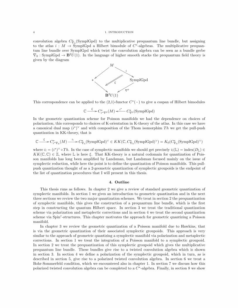
to the atlas i : M → SymplGpd a Hilbert bimodule of C∗-algebras. The multiplicative prequan-tum line bundle over SymplGpd which twist the convolution algebra can be seen as a bundle gerbe∇0 : SymplGpd → B2U(1). In the language of higher smooth stacks the prequantum field theory isgiven by the diagram
M
i
&&∗
""
SymplGpd
∇0xxB2U(1)
ξu
This correspondence can be applied to the (2,1)-functor C∗(−) to give a cospan of Hilbert bimodules
Cξ // C∗i∗∇0(M) C∗∇0(SymplGpd)
i∗oo
In the geometric quantization scheme for Poisson manifolds we had the dependence on choices ofpolarization, this corresponds to choices of K-orientation in K-theory of the atlas. In this case we havea canonical dual map (i∗)∨ and with composition of the Thom isomorphim Th we get the pull-pushquantization in KK-theory, that is
Cξ // C∗i∗∇0
(M)i! // C∗∇0
(SymplGpd)∨ ∈ KK(C, C∗∇0(SymplGpd)∨) = K0(C∗∇0
(SymplGpd)∨)
where i! = (i∗)∨ Th. In the case of symplectic manifolds we should get precisely i!(L) = index(DL) ∈KK(C,C) ∈ Z, where L is here ξ. That KK-theory is a natural codomain for quantization of Pois-son manifolds has long been amplified by Landsman, but Landsman focused mainly on the issue ofsymplectic reduction, while here the point is to define the quantization of Poisson manifolds. This pull-push quantization thought of as a 2-geometric quantization of symplectic groupoids is the endpoint ofthe list of quantization procedures that I will present in this thesis.
4. Outline
This thesis runs as follows. In chapter 2 we give a review of standard geometric quantization ofsymplectic manifolds. In section 1 we gives an introduction to geometric quantization and in the nextthree sections we review the two major quantization schemes. We treat in section 2 the prequantizationof symplectic manifolds, this gives the construction of a prequantum line bundle, which is the firststep in constructing the quantum Hilbert space. In section 3 we treat the traditional quantizationscheme via polarization and metaplectic corrections and in section 4 we treat the second quantizationscheme via Spinc-structures. This chapter motivates the approach for geometric quantizing a Poissonmanifold.
In chapter 3 we review the geometric quantization of a Poisson manifold due to Hawkins, thatis via the geometric quantization of their associated symplectic groupoids. This approach is verysimilar to the approach of geometric quantizing a symplectic manifold via polarization and metaplecticcorrections. In section 1 we treat the integration of a Poisson manifold to a symplectic groupoid.In section 2 we treat the prequantization of this symplectic groupoid which gives the multiplicativeprequantum line bundle. These bundles give rise to a twisted convolution algebra which is shownin section 3. In section 4 we define a polarization of the symplectic groupoid, which in turn, as isdescribed in section 5, give rise to a polarized twisted convolution algebra. In section 6 we treat aBohr-Sommerfeld condition, which we encountered also in chapter 1. In section 7 we discuss how thispolarized twisted convolution algebra can be completed to a C∗-algebra. Finally, in section 8 we show
4. OUTLINE 5
that this approach due to Hawkins reproduce the geometric quantization of symplectic manifolds andgive rise to the Moyal quantization of Poisson vector spaces.
In chapter 4 we discuss how the results of chapter 2 and 3 can be reinterpreted in terms of highergeometric quantization. To place us in the right setting we treat in section 1 3d Chern-Simons theoryas a motivating example. In section 2 we give a brief outline of the basic constructions and factsabout higher geometry and show how the prequantization steps of chapter 2 and 3 can be interpretedin higher prequantum geometry. In section 3 we show how this can interpreted in higher symplecticgeometry. We will show how the symplectic groupoid give rise to a degree 3-cocycle in the simplicialde Rham cohomology, how the non-degeneracy of this cocycle is encoded in the associated symplecticLie algebroid and how this gives rise to a Poisson σ-model. We will see also that this Poisson σ-modelcan be Lie integrated to a 2d Poisson-Chern-Simons theory which has the Poisson manifold as itsboundary theory. In section 4 we show that the higher geometric quantization of a 2d field theoryyields a 2-vector space of quantum 2-states, which has as 2-basis the algebra that we found in chapter3. These algebras make only sense up to Morita equivalence which reflects the fact that in highergeometry Lie groupoids make only sense up to Morita equivalence. This shows that the geometricquantization of Poisson manifolds as described in chapter 3 is not Morita faithful.
In chapter 5, we discuss the implications of this change of perspective and hint at a solution tothe problem that the results of chapter 3 are not Morita faithful. We conclude with an outlook forfurther research.

CHAPTER 2
Geometric Quantization of Symplectic Manifolds
In this chapter we give a review of standard geometric quantization of symplectic manifolds. Westart by explaining what geometric quantization is all about and what its difficulties are. There aretwo major quantization schemes which geometrically quantize symplectic manifolds and which dealwith these difficulties each in their own manner. The first step in both quantization schemes is theconstruction of some prequantum line bundle over the symplectic manifold, which one need in orderto define the actual quantum Hilbert space. In the first quantization scheme we review the traditionalquantization scheme via polarization and metaplectic corrections and in the second quantization schemewe review the more modern approach via Spinc-structures.
1. What is geometric quantization all about?
Traditionally, ”quantization” refer to the process which associates to a classical system its corre-sponding quantum system. The classical system is described by the commutative algebra of functionson the phase space of the system. Quantization associates to each classical system a Hilbert space H ofquantum states and defines a map Q from a subset of this commutative algebra to the space of opera-tors on H. Usually, the phase space is described by a symplectic manifold (M,ω) and the commutativealgebra is the Poisson algebra C∞(M). For a certain sub-algebra S ⊂ C∞(M) the quantization is theassignment
Q : S → Op(H)
mapping smooth functions f : M → R to operators Q(f) : H → H. One would like the following Diracaxioms to hold:
Q1: R-linearity: Q(rf + g) = rQ(f) +Q(g) ∀r ∈ R, f, g ∈ SQ2: Normalization: Q(1) = 1, where 1 is the constant function and 1 the identity operator on H.Q3: Hermiticity: Q(f)∗ = Q(f)Q4: Diracs quantum condition: [Q(f),Q(g)] = −i~Q(f, g)Q5: Irreducibility condition: If f1, ..., fk is a complete set of observables, then Q(f1), ...,Q(fk)
is a complete set of operators.
A set of observables f1, ..., fk is defined to be complete if the only observables which Poisson commutewith every element of f1, ..., fk are the constant functions. The set of operators is called completeif it acts irreducibly on H. By Schur’s lemma, this means in complete analogy that the only set ofoperators that commute with all of them are multiples of the identity (See [2, 9] for more detail).
There are many known examples of representations of Poisson subalgebras which do not complywith the irreducibility condition, for instance the so called prequantizations obtained through thegeometric quantization scheme. It is generally acknowledged that these examples are manifestations ofa general obstruction to quantization: it is impossible to quantize the entire Poisson algebra C∞(M)while satisfying simultaneously the Dirac quantum condition on the whole algebra and the irreducibilitycondition. This was first proved for R2n by the no-go theorem of Groenewald and van Hove [36, 44, 45]and later similar no-go results were proven for other symplectic manifolds [35].
Example 1.0.1. Let Q = Rn, M = T ∗Q with the standard symplectic form ω =∑dqj ∧ dpj ,
where qj are the coordinates of the configuration space Q and pj the corresponding momentum
7

8 2. GEOMETRIC QUANTIZATION OF SYMPLECTIC MANIFOLDS
coordinates in the fibers. Note that these coordinate functions qk and pl form a complete set ofobservables. Using the corresponding Poisson bracket
f, g =
n∑j=1
∂f
∂qj
∂g
∂pj− ∂f
∂pj∂g
∂qj
we require according to (Q4) the canonical commutation relations:
[Q(qk),Q(ql)] = [Q(pk),Q(pl)] = 0
[Q(qk),Q(pl)] = i~δkl
This means that the operators form the Heisenberg algebra and, by Schur’s lemma, (Q5) implies thatwe need to find an irreducible representation of this algebra. By the Stone-Von Neumann Theorem,any such representation (that exponentiates to a representation of the Heissenberg group) is unitarilyequivalent to L2(Q) = L2(Rn) with
Q(qk)ψ(x) = xkψ(x)
Q(pl)ψ(x) = −i~ ∂ψ∂xl
(x)
This gives us the famous Schrodinger representation.The fact that the wave function ψ(x) of the Hilbertspace L2(Q) depends only on the configuration space is a consequence of representation theory.
The kinetic energy p2 =∑pjpj can be represented by
Q(p2) = ~2∑ ∂2
∂xj∂xj= ~2∆
By imposing (Q3) and (Q4) one finds
Q(pkql) =
1
2
(Q(pk)Q(ql) +Q(ql)Q(pk)
)Which is known in quantum physics as operator ordening of Q(pkq
l) ∼ Q(pk)Q(ql). Note that ingeneral we have Q(fg) 6= Q(f)Q(g). It turns out that the quadratic observables form a closed Liealgebra under Poisson brackets, the symplectic Lie algebra sp(n). When we quantize a symplecticvector space, we always obtain a representation of the symplectic Lie algebra. We have now quantizedall the linear and quadratic observables in a consistent way. Unfortunately, we are unable to quantizecubic observables, hence even in the simplest case, no full quantization is possible[3].
Therefore the quantization procedure requires the selection of a preferred sub-algebra of C∞(M).There are no specific rules that tells us which complete set of observables to choose, nor is it ruled outthat different choices of complete sets will lead to different quantum theories with different physicalresults. It is here, where extraneous information and requirements enter the construction of a quantumtheory. Certain symmetries or geometric properties of the classical system make one complete set more’preferred’ than another. Geometric quantization is a procedure that addresses the question of existenceand classification of quantizations satisfying (Q1) through (Q5) in general.
2. Prequantization of a symplectic manifold
Geometric quantization is a quantization scheme which construct the Hilbert space H and themap Q from a symplectic manifold in a geometric way. This Hilbert space H will be defined as acertain subspace of the space of sections of a complex line bundle L over the symplectic manifold M .The construction of this line bundle is the first step towards geometric quantization, and is calledprequantization.

2. PREQUANTIZATION OF A SYMPLECTIC MANIFOLD 9
2.1. Line bundles and the first Chern characteristic class. We start by recalling a numberof standard definitions and results concerning line bundles and their first Chern characteristic classes.
Definition 2.1.1. Let M be a manifold. By a complex line bundle L over M , we mean a vectorbundle π : L→M with C, the complex numbers, as fibers.
Thus L is a manifold and the projection map π is smooth, and if for any p ∈ M one putsLp = π−1(p), then Lp is a one dimensional vector space over C. Moreover there exists a open coveringU = Ui|i ∈ I of M and nowhere vanishing smooth sections si : Ui → L on Ui, i ∈ I, such that themap ηi : C× Ui → π−1(Ui) given by ηi((z, q)) = zsi(q), is a diffeomorphism.
The set of pairs (Ui, si)|i ∈ I is called a local system for L. Given such local system, thecorresponding set of transition functions are the elements cij ∈ C∞(Ui ∩ Uj), i, j ∈ I defined bycijsi = sj on Ui ∩ Uj . This gives the relations
cij = c−1ji and cijcjk = cjk on Ui ∩ Uj ∩ Uk
We denote by Γ(L) the space of all smooth sections s : M → L, which form under pointwise multipli-cation a C∞(M)-module.
Two complex line bundles L1 and L2 over M are called equivalent if there exists a diffeomorphismτ : L1 → L2 such that for any p ∈ M , τ induces a linear isomorphism L1
p → L2p. This gives an equiv-
alence relation on the set of all line bundle over M and let L = L(M) be the set of these equivalenceclasses.
Let M be a smooth manifold and let U = Ui|i ∈ I be a open contractible cover of M , that iseach of the open sets Ui, Ui ∩Uj , Ui ∩Uj ∩Uk, ... is either empty or can be smoothly contracted to apoint.
A k-simplex is any k + 1-tuple (i0, i1, ..., ik) ∈ Ik+1 such that Ui0 ∩ Ui1 ∩ ... ∩ Uik 6= ∅. Let A bean abelian group. A k-cochain relative to U is any totally skew map
a : (i0, i1, ..., ik) 7→ a(i0, i1, ..., ik) ∈ Afrom the set of k-simplices into A. The set of all k-cochains form a abelian group Ck(U , A) underaddition of functions, and one obtains a group homomorphism δ : Ck(U , A)→ Ck+1(U , A) defined by
δa(i0, i1, ..., ik+1) =
k+1∑i=0
(−1)ja(i0, i1, ..., ij , ..., ik+1)
This δ is called the coboundary operator. Note that δ2 is trivial.A cochain a ∈ Ck(U ;A) such that δa = 0 is called a k-cocycle. If, in addition, a = δb for some
b ∈ Ck−1(U ;A) then a is called a k-coboundary. The set of k-cocycles is denoted by Zk(U ;A). Thek-coboundaries form a subgroup of Zk(U ;A) and the quotient
Hk(U ;A) =Zk(U ;A)
δ(Ck−1(U ;A))
is called the kth-cohomology group and defines the Cech cohomology of U , denoted by H(U ;A). If V is arefinement of U , then there is a homomorphism Hk(U ;A)→ Hk(V;A). Taking the inductive limit overall coverings under refinement, gives us the cohomology group Hk(M ;A). For any particular coveringU one has the natural homomorphism Hk(U ;A)→ Hk(M ;A), which is happens to be an isomorphismif U is contractible [33]. Thus we can identify Hk(U ;A) with Hk(M ;A), when U is contractible.
Now suppose that π : L → M is a complex line bundle and that Ui, si is a local system for L,with every Ui contractible. The transition functions cij : Ui∩Uj → C× form a Cech 1-cocycle, and thusL determines an equivalence class [c] ∈ H1(U ;C×). Furthermore if π1 : L1 →M and π2 : L2 →M are

10 2. GEOMETRIC QUANTIZATION OF SYMPLECTIC MANIFOLDS
two equivalent complex line bundles, with corresponding transition functions cij and bij respectively.
These two cocycles will be related by functions gi : Ui → C×, such that cij = gibijg−1j . This means
that cij and bij differ by the 0-coboundary, which shows that equivalent complex line bundles definethe same equivalence class in H1(M ;C×). Conversely, it can easily be shown that every one-cocycle in[c], will lead to equivalent complex line bundles[48]. The fact that the group H1(M ;C×) is isomorphicto H2(M ; 2πZ), follows from the long exact sequences in cohomology, coming from the short exactsequence of group homomorphisms
0→ 2πZ→ C→ C× → 0
where the map 2πZ → C is inclusion and the map C → C∗ is given by z 7→ eiz. With induced longexact sequence
...→ H1(M ;C)→ H1(M ;C×)ε→ H2(M ; 2πZ)→ H2(M ;C)→ ...→
implying H1(M ;C×) ∼= H2(M ; 2πZ), since H1(M ;C) = H2(M ;C) = 0 (C is contractible). If L iscomplex line bundle over M and β(L) is the corresponding element of H1(M ;C×), then the equivalenceclass c1(L) = 1
2π εβ(L) ∈ H2(M ;Z) is called the first Chern characteristic class of L[48].
Consider a complex line bundle π : L→M . For any k ∈ N, let
Ωk(M,L) = Γ(M,L⊗ ∧k(T ∗M))
be the space of k-forms with values in L.
Definition 2.1.2. A Hermitian metric on L is an Hermitian inner product 〈·, ·〉 on each fiber withthe property that, for any s, t ∈ Γ(L), the function 〈s, t〉 : M → C defined by m 7→ 〈s(m), t(m)〉 issmooth.
Definition 2.1.3. A connection of L is a linear map ∇ : Ω0(M,L)→ Ω1(M,L) satisfying
∇(fs) = df ⊗ s+ f∇sfor any section s ∈ Γ(M,L) and function f ∈ C∞(M).
These two structures are required to be compatible if we have
d〈s, t〉 = 〈∇s, t〉+ 〈s,∇t〉, ∀s, t ∈ Γ(M,L)
Definition 2.1.4. A complex line bundle with connection ∇ and a compatible Hermitian metricis called a Hermitian line bundle with connection and is denoted by (L, 〈·, ·, 〉,∇).
Example 2.1.5. Let L be the trivial bundle M × C, so that Ωk(M,L) = Ωk(M). Then for anyβ ∈ Ω1(M), we can define a connection ∇ by
∇f = df + fβ, f ∈ C∞(M)
Conversely, all the connections of the trivial bundle have this form, since we can set β = ∇1 andcompute ∇(f 1) = df + f∇1.
Given a connection ∇ of a complex line bundle L on M and a vector field X of M , then thecovariant derivative with respect to X is defined by
∇X : Γ(M,L)→ Γ(M,L) ∇Xs = ∇s(X)
If (U, s) is a pair of a local system and β = ∇ss , then ∇X(fs) = Xf ⊗ s+β(X)⊗ s. Furthermore there
exist an ω ∈ Ω2(M) such that for any vector fields X,Y we have
ω(X,Y ) = ∇x∇Y −∇Y∇X −∇[X,Y ]
which is called the curvature of ∇.

2. PREQUANTIZATION OF A SYMPLECTIC MANIFOLD 11
Let M be a smooth manifold with an open contractible cover U , then it can be shown that the Cechcohomology H(M ;R) is precisely isomorphic to the de Rham cohomology HdR(M ;R)[83]. Considerin addition an Hermitian line bundle with connection (L, 〈·, ·, 〉,∇) on M , then the curvature of thisconnection ∇ defines a 2-form which de Rham class is an element of H2
dR(M ;R). This de Rham classof the curvature of the Hermitian line bundle L is closely related to the first Chern charactersitic classof L. The first Chern class c1(L) maps to 1
2π [ω] under the natural homomorphism
i : H2(M ;Z)→ H2(M ;R)
Consequently 12π [ω] has to be integral[83]. For the converse we have the following result due to Weil
(see [48]).
Theorem 2.1.6. (Weil’s theorem) Let σ be a closed 2-form on smooth manifold M such that itsde Rham cohomology class lies in the image of i : H2(M ;Z) → H2(M ;R). Then there exists anHermitian line bundle with connection (L, 〈·, ·, 〉,∇) on M such that its curvature equals 2πσ.
The ker i is exactly the torsion subgroup of H2(M ;Z), that is the Hermitian line bundle withconnection (L, 〈·, ·, 〉,∇) is determined by [σ] uniquely up to torsion element of H2(M ;Z).
2.2. Prequantum line bundle. This theorem of Weil gives us a prequantization condition for asymplectic manifold (M,ω). A symplectic manifold (M,ω) is called prequantizable if 1
2π [ω] is integral.Which gives the following definition:
Definition 2.2.1. A prequantization of (M,ω) is a Hermitian line bundle with connection (L, 〈, 〉,∇)such that the curvature of the connection ∇ is ω. We call L a prequantum line bundle on (M,ω).
This formulation is due to Kostant, an equivalent formulation is made by Souriau by using principalU(1)-bundles associated to L. Recall that a principal U(1)-bundle consists of a fiber bundle π :P → M with fiber U(1) and for any x ∈ M , an action of U(1) on Px which is free and transitive.Furthermore P need to be locally trivializable, that is for any x ∈ M there exists a neighborhood Uand a diffeomorphism φ : π−1(U)→ U ×U(1) such that φ(p) = (π(p), τ(p)), where τ : π−1(U)→ U(1)satisfy τ(θ · p) = θ + τ(p) for θ ∈ U(1). For any θ ∈ U(1) we denote the action by Lθ : P → P , thenthe vector field ∂θ of P is given by
∂θ|p =d
dt|t=0Lt(p)
for p ∈ P . A connection on a principal U(1)-bundle π : P → M is a 1-form Θ ∈ Ω1(P,R) whichis U(1)-invariant, i.e. L∗θΘ = Θ for any θ ∈ U(1), and satisfies ι∂θΘ = 1. These two conditions onΘ imply that there exist a unique 2-form ω ∈ Ω2(M ;R) such that π∗ω + dΘ = 0, which is calledthe curvature of Θ. Given an Hermitian line bundle (L, 〈, 〉), the associated principal U(1)-bundleis given by P = v ∈ L|〈v, v〉 = 1. Conversely, to a principal U(1)-bundle P we can associatethe Hermitian line bundle L = P ×U(1) C. The prequantization (L, 〈, 〉,∇) uniquely determines the
prequantization (P,Θ) and vice verse, via the equation ∇ss =
√−1s∗Θ for every s ∈ Γ(P ) ⊂ Γ(L).
Hence a prequantization of (M,ω) is a principal U(1)-bundle π : P →M equipped with a connectionθ on P such that the curvature of this connection is ω.
Example 2.2.2. Let ω be an exact 2-form on M and let β be a 1-form on M such that dβ = −ω.Then (M,ω) can always be prequantized by the trivial U(1)-bundle P = M × U(1) and connectionΘ = dθ + π∗β, where θ : P → U(1) is the the angle coordinate on U(1).
A map of Hermitian line bunles τ : L′ → L, is a diffeomorphism which, (i) commutes with theprojection π τ = π′, (ii) it restricts to a linear isomorphism τm : L′m → Lm for each m ∈M and (iii)the functions H ′ : L′ → R, H : L→ R defined by H ′(s) = 〈s, s〉′, H(s) = 〈s, s〉 satisfy H τ = H ′. IfL′ = L, then we call τ a gauge transformation/equivalence. If in addition ∇ is a connection on L, thenwe require that τ∗(∇) = ∇ in order for τ to be an gauge transformation of (L, 〈, 〉,∇). Analogously,

12 2. GEOMETRIC QUANTIZATION OF SYMPLECTIC MANIFOLDS
a map of principal U(1)-bundles φ : P ′ → P , is a smooth map of manifolds which commutes withthe U(1)-action. If P ′ = P , then we call φ a gauge transformation/equivalence. If in addition Θ is aconnection on P , then we require that φ∗(Θ) = Θ in order for φ to be an gauge transformation of (P,Θ).Two prequantization (L, 〈, 〉,∇) are gauge equivalent if and only if the corresponding prequantizations(P,Θ) are gauge equivalent. Since a gauge equivalence is an isomorphism of bundles that respectsadditional structures, we will be interested in prequantum line bundles up to gauge equivalence. Dueto Kostant we have the following result:
Proposition 2.2.3. [48] Let (M,ω) be a symplectic manifold, such that the cohomology class1
2π [ω] is integral. Let (L, 〈, 〉,∇) be a prequantum line bundle. Then for every Hermitian structure 〈, 〉′on L there is a prequantization (L, 〈, 〉′,∇′) for (M,ω). If M is simply connected, the prequantizationstructure on L is unique up to gauge equivalence. More generally the prequantization structures on Lare classified by H1(M ;R)/H1(M ;Z), up to gauge equivalence.
A consequence is that if M is simply connected ,then all connections Θ with dΘ = −π∗ω areequivalent by gauge transformations.
Remark 2.2.4. If the classical system has a symmetry group G, then it is natural to require thatthe quantum system obtained also posses this symmetry. A Hamiltonian G-action on a symplecticmanifold (M,ω) with associated moment map Φ, gives rise to a linear group action on the associatedHilbert space H. The irreducibility condition can be reformulated by saying that the quantizationof a transitive Hamiltonian G-action is an irreducible G-representation. This leads to the famousOrbit method, developed by Kirillov and Kostant [47, 48], which gives a quantization procedurefor constructing an irreducible unitary representation of the group G starting from a G-orbit in thecoadjoint representation. For more details, see [32].
3. Geometric quantization by polarization
The space of smooth sections of L is too large for geometric quantization. As we saw in example1.0.1, the Hilbert space L2(Q) depends only on the configuration space Q, and not on the state spaceT ∗Q. This Hilbert space space can be thought of as functions on T ∗Q which are independent of thefiber variables. To cut down the variable dependency of the functions by half, is known as polarization.A choice of polarization is what in physics is called a choice of ”canonical coordinates” and ”canonicalmomenta”, where the canonical momenta are the coordinates along a leaf and the canonical coordi-nates are the coordinates on the leaf space. The advantage of restricting to a smaller class of sections,namely the ”polarized sections”, is that the resulting prequantization may satisfy the ”irreducibilityaxiom” of section 1. The space of smooth sections of L is just too big for this axiom to hold. In thelanguage of physics these polarized sections are called ”wave functions” and the polarization condi-tion says precisely that these wave functions are functions on the phase space which depend only oncanonical coordinates and not on canonical momenta.
3.1. Polarization. Recall that a complex distribution is a complex subbundle F ⊂ TCM =TM⊗C. If (M,ω) is symplectic, F is called Lagrangian if for every p ∈M the subspace Fp ⊂ TpM⊗Cis Lagrangian, i.e. dimC Fp = 1
2 dimM and the complex-valued two-form induced from ω vanishes onFp. A distribution F is said to be involutive if for any two vector fields u and v of F , the Lie bracket[u, v] is also a vector field of F . A distribution F is said to be integrable if for all p ∈ M there is asubmanifold S ⊂ M such that p ∈ S and for all q ∈ S we have TqS = Fq. By Frobenius theorem adistribution F is involutive if and only if it is integrable.
Definition 3.1.1. A polarization of a symplectic manifold (M,ω) is a complex involutive La-grangian distribution F ⊂ TCM .

3. GEOMETRIC QUANTIZATION BY POLARIZATION 13
Definition 3.1.2. A real polarization is an involutive Lagrangian real distribution F ⊂ TM . Apolarization F is called totally complex (or Kahler) if F ∩F = 0.
If a polarization satisfies F = F , then it is the complexification of a real polarization and hencewe regard a real polarization as a special case of complex polarization.
Example 3.1.3. A real polarization F is an integrable subbundle of TM . Frobenius theoremstates that it defines a foliation of M , whose leaves are Lagrangian submanifolds of M . Conversely,every Lagrangian foliation defines a real polarization.
A real polarization may not exist in general. For example, on a two-dimensional surface a realpolarization corresponds to a nowhere vanishing vector field, thus if the two-sphere S2 has a realpolarization then it has a nowhere vanishing vector field, which contradicts the well-known Hairy balltheorem. This is why we consider involutive Lagrangian distributions of the complexified tangentbundle.
Example 3.1.4. For (M,J) an almost complex manifold. The almost complex structure J : TM →TM extends to a C-linear bundle isomorphism on TCM and has eigenvalues ±i. The ±i eigenspaces ofJ are denoted by T1,0M and T0,1M and are spanned by vectors of the form X ∓ iJX. These bundlesare complex conjugate of each other and satisfy T1,0M ∩ T0,1M = 0, hence TCM = T1,0M ⊕ T0,1M .The distribution T0,1M is Lagrangian if and only if the symplectic form ω is of type (1,1), that isω ∈ Ω1,1(M). The fact that ω is a (1,1)-form implies that 〈u, v〉 := ω(u, Jv) is a symmetric metric.If we require in addition that this symmetric metric is positive definite, then we say that the almostcomplex structure J is compatible with ω. By the Newlander-Nirenberg theorem, the distributionT0,1M is integrable if and only if J comes from a complex structure on M . In this case we call (M,J, ω)a Kahler manifold, which is a symplectic manifold with an integrable almost complex structure whichis compatible with the symplectic form. For Kahler manifolds we have the natural polarization T0,1M ,which is called the Kahler polarization. Conversely, every Kahler polarization F give rise to an almostcomplex structure J on M , with the property that at a point x ∈ M , the vector X + iJX, forall X ∈ TxM , span the space Fx. By Newlander-Nirenberg theorem this J comes from a complexstructure on M , and if in addition this J is compatible with ω, then it defines a Kahler manifold(M,J, ω) (See [90]).
In general for a polarization F , the real part F ∩TM is not necessarily of constant rank. Byrequiring that it is of constant rank ensures us that it is an involutive distibution, i.e. a foliation. Butthe subbundle F +F ⊂ TCM is still not necessarly involutive. Imposing the following conditions on Fensures us that the polarization is well behaved.
Definition 3.1.5. For a polarization F ⊂ TCM , the distributions D,E ⊂ TM are defined byDC := F ∩F and EC := F +F . The polarization F is strongly admissible if there exist manifolds andsurjective submersions
MpM/D
qM/E
such that D and E are the kernel foliations D = kerTp and E = kerT (q p).
Example 3.1.6. A polarization satisfying F = F is the complexification of a real polarization.For such a polarization D = E, so that F = DC is strongly admissible if the space of leaves of theunderlying real polarization D are smooth manifolds. For a Kahler polarization we have F ∩F = 0so D = 0 and hence E = TM , since D⊥p = Ep for all p ∈ M , so that any Kahler polarization isstrongly admissible.
In geometric quantization, one starts with a symplectic manifold (M,ω), together with a prequan-tization (L, 〈, 〉,∇) and a polarization F . Further we assume that F is strongly admissible. A sections ∈ Γ(L) is covariantly constant along F if ∇Xs = 0 for all X ∈ Γ(F). We denote the space of sections

14 2. GEOMETRIC QUANTIZATION OF SYMPLECTIC MANIFOLDS
of L covariantly constant along a polarization F by ΓF (L), which is also called the space of polarizedsections.
Example 3.1.7. (Vertical polarization) Let Q be a manifold, and M = T ∗Q be its cotangentbundle, with projection map πQ : T ∗Q → Q. The tautological one-form τ can locally be defined asτ =
∑pidqi, with the canonical symplectic form ω = −dτ =
∑dqi ∧ dpi. Let F ⊂ TCM be the
subbundle
F := kerTCπQ ∼= TCQ → TCM
Then F is a polarization of (M,ω), called the vertical polarization. In fact it is a real polarization,which is strongly admissible. Now M can be quantized by the trivial Hermitian line bundle L = M×C,with Hermitian metric (α, β) = α∗β for α, β ∈ Γ(L) and connection ∇ = d + iτ ,where ∇X = ιX∇.The curvature of this connection is ω = −dτ . The sections of L are functions s : T ∗Q → C and foreach vertical vector field X ∈ Γ(F), we have that ∇Xs = ιXds = LX s = 0. Hence the polarizedsections are functions on T ∗Q which are constant on the fibers. i.e. the pullback of functions on Q toT ∗Q.
Example 3.1.8. (Kahler polarization) Let (M,J, ω) be a Kahler manifold. We saw in example3.1.4 that we have a natural Kahler polarization T0,1M . If we have in addition a prequantum linebundle (L, 〈, 〉,∇) for M , then L becomes a holomorphic line bundle and its polarized sections areexactly the holomorphic sections. To see this, first note that ω is of type (1,1) and closed, we haveby the local exactness of the Dolbeault complex (see [90]) that there exists a (1,0)-form τ such thatω = ∂τ on some neighborhood around p ∈ M . This τ satisfies ∂τ = 0, since ∂(∂τ) = −∂ω = 0and again by local exactness there exists a form α such that ∂τ = ∂α on some neighborhood aroundp. Since ∂τ is of type (2,0) and ∂α is of type (1,1), we must have that ∂τ = 0. This means thatdτ = ∂τ + ∂τ = ω. Locally we can trivialize the prequantum bundle L, by passing to a smaller openU around p, such that the connection has the form ∇ = d− iτ , where ω = dτ . By taking a constantsection s of L, i.e. LX s = ds(X) = 0 for X ∈ Γ(TM), we have that
∇ss
= −iτ(3.1)
This section s is unique, since an arbitrary section of L is of the form fs, where f ∈ C∞(M), and forthis section condition (3.1) implies that df = 0, and hence f is constant. By assuming without lossof generality that U is a simply connected, proposition 2.2.3 implies that for every prequantum linebundle (L, 〈, 〉,∇) on M we have a unique trivializing section s of L such that condition (3.1) holds.Since τ is op type (1,0) we have that
∇ ∂∂zi
s = −iτ(∂
∂zi)s = 0
on U , with local coordinates zi where i = 1, ..., n. Hence this s is a local holomorphic section of L overU and this gives a well-defined holomorphic structure on L, which makes L a holomorphic line bundle.Furthermore the polarized sections of L over U is the product of s with a holomorphic function, hencethe polarized sections are exactly the holomorphic sections.
By polarization we restricted to a smaller class of sections, namely the polarized sections. Toobtain a Hilbert space we might be tempted to define this Hilbert space as the densely spanned spaceof polarized sections. The pitfall is that these polarized sections are covariantly constant along theleaves of D and if these leaves are noncompact, then these polarized sections are not square integrablewith respect to the volume form ωn. A remedy to this problem is to integrate the polarized sectionsnot over M but over the space M/D of leaves of the polarization. However there is no natural volumeform on M/D. You can tackle this problem by working with ”half-densities” or with ”half-forms”.

3. GEOMETRIC QUANTIZATION BY POLARIZATION 15
3.2. Half-form bundle. We will tackle this problem by using the approach via ”half-forms”.Normally, if we want to integrate a volume form over a smooth manifold, we know that the ”change ofvariables” formula for integration involves absolute values of Jacobians, hence integration of n-formson M require the choice of orientation. The use of densities will circumvent this need, however in morecomplex systems the use of n-forms seems more suitable.
Let M be a manifold of dimension n. We can think of an n-form ν on M as a function which atx ∈M assigns to each basis e1, ..., en of TxM a number that satisfies
ν(eg) = det(g) · ν(e)
for all g ∈ GL(n,R) and where e = e1 ∧ ...∧ en. Similarly, an α-density is defined as an object ν whichchanges according to
ν(eg) = |det(g)|α · ν(e)
We would like to define a half-form as an object which changes according to
ν(eg) = det(g)1/2 · ν(e)
The problem is that det(g)1/2 is not a well-defined function on GL(n,R) and to remedy this we needto pass to a double covering of GL(n,R) and a corresponding double covering of the bundle of bases ofTM . This double covering of the frame bundle is called a metalinear frame bundle. But before we con-struct this bundle let us first start with the definition of the double covering of the general linear group.
The general linear group GL(n,R) has two components, namely the matrices of positive andnegative determinants. We expect that the double covering we are looking for should have fourcomponent and that det(g)1/2 should take values in the half lines R+, iR+, −R+ and −iR+. It willbe convenient to regard GL(n,R) as a subgroup of real matrices lying in GL(n,C).
Consider the group isomorphism
π : (C× SL(n,C))/Z∼=→ GL(n,C)
given by (z,A) 7→ ezA, where the action of k ∈ Z on (z,A) is given by (z + 2πikn , e−
2πikn A). We
have the map det : GL(n,C) → C∗ and this pulls back to the map det π on C × SL(n,C), wheredet π(z,A) = enz and this has a well-defined holomorphic square root
χ(z,A) :=√
det π(z,A) = enz2
which is defined on the group ML(n,C) := (Z× SL(n,C))/2Z, which we call the complex metalineargroup. It is a double cover of GL(n,C), with as double covering map r : ML(n,C) → GL(n,C) theprojection of ML(n,C) to GL(n,C), so that
χ2(z,A) = det r(z,A)
If we regard GL(n,R) → GL(n,C) as the real matrices, then we obtain the real metalinear groupML(n,R) as a double cover of GL(n,R). Indeed it follows that χ can take on values in the four halflines R+, iR+, −R+ and −iR+ and thus the group ML(n,R) has four components[37].
Definition 3.2.1. Let p : P → M be a vector bundle of finite rank n. Its frame bundle is thebundle F (P ) → M over the same base, whose fiber over x ∈ M is the set of all ordered bases ofPx = p−1(x).
The frame bundle has a natural action of GL(n,K), where K denotes the ground field, given byan ordered change of basis which is free and transitive, i.e. the frame bundle is a principal GL(n,K)-bundle.
16 2. GEOMETRIC QUANTIZATION OF SYMPLECTIC MANIFOLDS
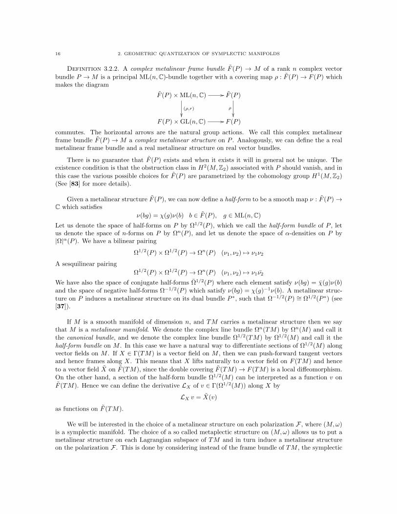
Definition 3.2.2. A complex metalinear frame bundle F (P ) → M of a rank n complex vector
bundle P →M is a principal ML(n,C)-bundle together with a covering map ρ : F (P )→ F (P ) whichmakes the diagram
F (P )×ML(n,C)
(ρ,r)
// F (P )
ρ
F (P )×GL(n,C) // F (P )
commutes. The horizontal arrows are the natural group actions. We call this complex metalinearframe bundle F (P )→M a complex metalinear structure on P . Analogously, we can define the a realmetalinear frame bundle and a real metalinear structure on real vector bundles.
There is no guarantee that F (P ) exists and when it exists it will in general not be unique. Theexistence condition is that the obstruction class in H2(M,Z2) associated with P should vanish, and in
this case the various possible choices for F (P ) are parametrized by the cohomology group H1(M,Z2)(See [83] for more details).
Given a metalinear structure F (P ), we can now define a half-form to be a smooth map ν : F (P )→C which satisfies
ν(bg) = χ(g)ν(b) b ∈ F (P ), g ∈ ML(n,C)
Let us denote the space of half-forms on P by Ω1/2(P ), which we call the half-form bundle of P , letus denote the space of n-forms on P by Ωn(P ), and let us denote the space of α-densities on P by|Ω|α(P ). We have a bilinear pairing
Ω1/2(P )× Ω1/2(P )→ Ωn(P ) (ν1, ν2) 7→ ν1ν2
A sesquilinear pairing
Ω1/2(P )× Ω1/2(P )→ Ωn(P ) (ν1, ν2) 7→ ν1ν2
We have also the space of conjugate half-forms Ω1/2(P ) where each element satisfy ν(bg) = χ(g)ν(b)and the space of negative half-forms Ω−1/2(P ) which satisfy ν(bg) = χ(g)−1ν(b). A metalinear struc-ture on P induces a metalinear structure on its dual bundle P ∗, such that Ω−1/2(P ) ∼= Ω1/2(P ∗) (see[37]).
If M is a smooth manifold of dimension n, and TM carries a metalinear structure then we saythat M is a metalinear manifold. We denote the complex line bundle Ωn(TM) by Ωn(M) and call itthe canonical bundle, and we denote the complex line bundle Ω1/2(TM) by Ω1/2(M) and call it thehalf-form bundle on M . In this case we have a natural way to differentiate sections of Ω1/2(M) alongvector fields on M . If X ∈ Γ(TM) is a vector field on M , then we can push-forward tangent vectorsand hence frames along X. This means that X lifts naturally to a vector field on F (TM) and hence
to a vector field X on F (TM), since the double covering F (TM)→ F (TM) is a local diffeomorphism.On the other hand, a section of the half-form bundle Ω1/2(M) can be interpreted as a function v on
F (TM). Hence we can define the derivative LX of v ∈ Γ(Ω1/2(M)) along X by
LX v = X(v)
as functions on F (TM).
We will be interested in the choice of a metalinear structure on each polarization F , where (M,ω)is a symplectic manifold. The choice of a so called metaplectic structure on (M,ω) allows us to put ametalinear structure on each Lagrangian subspace of TM and in turn induce a metalinear structureon the polarization F . This is done by considering instead of the frame bundle of TM , the symplectic

3. GEOMETRIC QUANTIZATION BY POLARIZATION 17
frame bundle Bp(M) consisting of all symplectic frames of TM . A symplectic frame at each x ∈ Mis an ordered basis e1, ..., en, f1, ..., fn such that ω(ei, ej) = ω(fi, fj) = 0 and ω(ei, fj) = δij for alli, j ≤ n. The collection of symplectic frames at x ∈M is equivalent to the symplectic group Sp(n,R),i.e. the group of real 2n× 2n-matrices of the block form
S =
(A BC D
)with A,B,C,D n× n-matrices and satisfying STσS = σ, where σ =
(0 1−1 0
). Notice that GL(n,R)
is naturally embedded in Sp(n,R) via the map sending g ∈ GL(n,R) to(g 00 (g−1)T
)in Sp(n,R). As is explained in [37] Sp(n,R) is diffeomorphic to the product of the unitary groupU(n) and an Euclidean space. Therefore the fundamental group of Sp(n,R) is Z so that Sp(n,R)has a unique double covering, which we denote by Mp(n,R) and we call the metaplectic group. Notethat the symplectic frame bundle Bp(M) has a canonical right action of Sp(n,R) and similar to theconstruction of the metalinear frame bundle we can now construct the metaplectic frame bundle.
Definition 3.2.3. A metaplectic frame bundle Mp(M) → M is a principal Mp(n,R)-bundletogether with a covering map ρ : Mp(M)→ Bp(M) which makes the diagram
Mp(M)×Mp(n,R)
(ρ,r)
// Mp(M)
ρ
Bp(M)× Sp(n,R) // Bp(M)
commutes. The horizontal arrows are the natural group actions. We call this metaplectic frame bundleMp(M) → M a metaplectic structure on M . The choice of a metaplectic structure on a symplecticmanifold (M,ω) is also called a metaplectic correction.
Of course, such a lifting may not exist and if it exist it may not be unique. A symplectic manifold(M,ω) together with a metaplectic structure determines a metalinear structure for each Lagrangiansubbundle of TM and hence on each polarization of M (See [37] for more details).
Now if we consider symplectic manifold (M,ω) together with a metaplectic structure and a realpolarization F ⊂ TM that is strongly admissible, then we have a surjective submersion p : M →M/D,where M/D is the space of integral surfaces. Now if we pull-back T ∗(M/D) to M along p, we get the
annihilator bundle of F , which we denote by F⊥. That is
F⊥ := ξ ∈ T ∗M : ∀X ∈ F , 〈X, ξ〉 = 0
At each x ∈M we have that Fx is the annihilator space of F⊥x and since Fx is Lagrangian, it is alsothe annihilator space of its image under the isomorphism of TM with T ∗M given by the symplecticform ω, hence this gives an isomorphism F (F)x with F (T ∗(M/D))p(x). The metaplectic structure onM induces a metalinear structure on Fx, which in turn induce a metalinear structure on T ∗(M/D)p(x)
The metalinear structure on T ∗(M/D)p(x) is obtained by covering the frame bundle F (T ∗(M/D))p(x)
by the bundle F (F)x, via the isomorphism of Fx with T ∗(M/D)p(x). This is independent of the choice
of a point in the fiber p−1(y), y ∈M/D, and does give a bundle covering of F (T ∗(M/D)). A smooth
section v of F (F) is constant along a section X of F if it satisfies LX v = 0. These sections gives a
section of F (T ∗(M/D)) and in this way we get a metalinear structure on M/D. Hence we can identifythe half-forms Ω1/2(M/D) with those sections of Ω−1/2(F) that are constant along F (See [37] for
18 2. GEOMETRIC QUANTIZATION OF SYMPLECTIC MANIFOLDS
more details). Since F is in particular an involutive distribution, we have a Bott connection on F⊥,that is the flat F-connection which equals the Lie derivative, i.e. ∇BXv := LX v for any X ∈ Γ(F)
and v ∈ Γ(F⊥). This Bott connection extends to any bundle constructed from F⊥. By duality the
half-form Ω1/2(F⊥) is equal to Ω−1/2(F) and hence the induced Bott connection on Ω1/2(F⊥) inducesa connection on Ω−1/2(F), which correspond to our previous defined Lie derivative along F . Hence
we can identify the half-forms of Ω1/2(M/D) with those sections of Ω1/2(F⊥) that are F-constant bythe Bott connection.
Combining the connection ∇ of a prequantum line bundle L and the Bott connection gives a flatF-connection ∇ on L⊗Ω1/2(F⊥). Define a section of L⊗Ω1/2(F⊥) to be polarized if it is F-constant
by this connection, i.e. a sections s ⊗ v ∈ Γ(L ⊗ Ω1/2(F⊥)) needs to satisfy ∇Xs = 0 and LX v = 0for all X ∈ Γ(F). The inner product of two polarized sections gives a volume form, which can beintegrated over M/D. This gives the pre-Hilbert space, consisting of all square integrable polarized
sections of L⊗Ω1/2(F⊥). The completion of this space gives us the quantum Hilbert space L2F (M,L).
[83].Now if we consider a polarization F ⊂ TCM that is not real, then the inner product is valued in
Ω1/2(F⊥)⊗ Ω1/2(F⊥), rather than Ωn(D⊥C ). Instead one has the natural isomorphism[39]
Ωn(F⊥)⊗ Ωn(F⊥) ∼= Ωn(E⊥C )⊗ Ωn(D⊥C )
and the exterior product with ωk
k! , with 2k := rkE−rkD, defines a canonical isomorphism Ωn/2(D⊥) ∼=Ωn/2(E⊥). With these isomorphisms we can correct the inner product and define L2
F (M,L) for everypolarization F .
3.3. Bohr-Sommerfeld variety. There are some complications involved if the leaves of the po-larization are not simply connected, which lead to the notion of a Bohr-Sommerfeld variety. Let Λ bean integral manifold of D. Then the flat F-connection ∇ on L⊗Ω1/2(F⊥) induces a flat F-connection
on the restriction of L ⊗ Ω1/2(F⊥) to Λ. The holonomy group GΛ of this connection is a subgroupof C×. Now if Λ is not simply connected, then it is possible to have non-trivial holonomy along thenon-contractible loops in Λ. Now since a section s⊗ v|Λ is a covariantly constant section, it does notchange under parallel transport, and in particular, cannot pick up a phase from the non-trivial holo-nomy group GΛ. Therefore either s⊗ v|Λ is the zero section or the holonomy group GΛ is trivial, i.e.GΛ = 1. Now we call the union of all integral manifolds of D such that GΛ = 1 the Bohr-Sommervariety MB-S . Hence in practice we restrict M to the Bohr-Sommerfeld variety MB-S . In the case thatall Λ are simply connected we have that M = MB-S [3].
Another difficulty is that it seems that our constructed quantum Hilbert space could be zero,depending on the topology of the integral surfaces of F . A solution may be given using ”cohomologicalwave functions”, where the local polarized section of Ω1/2(F⊥) form a sheaf (see [93]). The globalpolarized sections corresponds to the zeroth sheaf cohomology space, but the higher sheaf cohomologyspaces may not be zero. This hints to a relation between the quantum Hilbert space and highercohomology spaces. In Spinc-quantization, which we treat in the next section, we will consider thequantum Hilbert space as the index of a Spinc-Dirac operator acting on a certain chain complex. ForSpinc-quantization you need instead of the choice of a metaplectic structure, the choice of a Spinc-structure. The notion of a metaplectic structure is closely related to the notion of Spinc-structure, theadvantage of Spinc-structures is that the space of all choice is very well understood. Furthermore, thismay also allow us to describe the quantization of a symplectic manifold with a Hamiltonian G-action asa G-representation on a virtual vector space. In this setting Spinc-quantization can also be describedby a pushforward map in equivariant K-theory, as was first observed by [61].
4. GEOMETRIC QUANTIZATION BY Spinc-STRUCTURES 19
4. Geometric quantization by Spinc-structures
In the previous section we constructed the Hilbert space of quantum states as a certain subspaceof the space of polarized sections of L⊗Ω1/2(F⊥). There is a second quantization scheme, that seemsto be more natural and general from a mathematical point of view. In this case we need to choose,instead of a metaplectic structure, a Spinc structure. This define the Hilbert space of quantum statesas the index of a corresponding Dirac operator twisted by L. Let us start with the case of Kahlerpolarization, since this fits completely within the framework of complex geometry.
4.1. Quantization of the Dolbeault-Dirac operator. Let (M,ω) be a compact symplecticmanifold and let (L, 〈, 〉,∇) be a prequantization of (M,ω). Let J be an almost complex structureon TM that is compatible with ω, i.e. the symmetric bilinear form g := ω(−, J−) is a Riemannianmetric on M . Notice that every symplectic manifold admits an almost complex structure J that iscompatible with the symplectic form[32]. This defines the Hermitian metric h := g + iω on M andgive rise to an Hermitian inner product h0,1 on the vector bundle T 0,1M := T ∗0,1M . Remember fromexample 3.1.4, that the almost complex structure J give rise to a splitting TCM = T1,0M ⊕ T0,1M .This Hermitian inner product is constructed using the composition of the induced complex linearisomorphism h : TxM → T ∗xM and i : T ∗xM → T 0,1M , from where we can construct a unitary framelocally on T 0,1M . This in turn gives us a Hermitian inner product on T 0,qM := ∧qT 0,1M . Similarly wehave an Hermitian inner product on T p,0M . The choice of a metaplectic structure on M gives us also aHermitian inner product on Ω1/2(T 1,0M). Since L is by construction equipped with a Hermitian inner
product, one has a Hermitian inner product hL⊗T 0,qM on L ⊗ T 0,qM , where L = L ⊗ Ω1/2(T 1,0M).
These Hermitian inner products and the volume form ωn give an Hermitian L2-inner product of twosections u and v of L⊗ T 0,qM , which is defined as
(u, v) =
∫M
hL⊗T 0,qM (u, v)ωn
The connection ∇ on L and the Bott connection on Ω1/2(T1,0M) gives the flat T0,1M -connection
∇ on L and defines a differential operator
∇ : Ωk(M ; L)→ Ωk+1(M ; L)
such that for all s ∈ Γ(M ; L) and α ∈ Ωk(M) , ∇(s⊗ α) = ∇s⊗ α+ s⊗ dα. Consider the projection
π0,∗ : Ω∗C(M ; L)→ Ω0,∗(M ; L)
according to the decomposition ΩkC(M ; L) =⊕
p+q=k Ωp,q(M ; L). Define the differential operator
∂ : Ω0,q(M ; L)→ Ω0,q+1(M ; L)
by
∂ := π0,∗ ∇The formal adjoint ∂
∗of ∂ is the differential operator
∂∗
: Ω0,q(M ; L)→ Ω0,q−1(M ; L)
defined by the above Hermitian L2-inner product as
(∂(u), v) = (u, ∂∗(v)), u ∈ Ω0,q(M ; L), v ∈ Ω0,q+1(M ; L)
Definition 4.1.1. The Dolbeault-Dirac operator is the elliptic differential operator
∂ + ∂∗
: Ω0,∗(M ; L)→ Ω0,∗(M ; L)
which maps even degree forms to odd degree, and vice versa.

20 2. GEOMETRIC QUANTIZATION OF SYMPLECTIC MANIFOLDS
The Dolbeault-quantization of (M,ω) is defined as the virtual vector space[10]
Q(M) =∑
(−1)kH0,k(M ; L)
which is by Hodge theory, the index of the Dolbeault-Dirac operator
∂ + ∂∗
: Ω0,even(M ; L)→ Ω0,odd(M ; L)
. In other words,
Q(M) = ker(∂ + ∂∗)− coker(∂ + ∂
∗)
This index is well-defined, because this operator is elliptic and M is compact. Note that we have
coker((∂ + ∂∗)|Ω0,even(M ;L))
∼= ker((∂ + ∂∗)|Ω0,odd(M ;L)) hence
Q(M) = ker((∂ + ∂∗)|Ω0,even(M ;L))− ker((∂ + ∂
∗)|Ω0,odd(M ;L))
Remark 4.1.2. When M is compact the Dolbeault quantization is independent of the choice of J(See [32]).
This definition of quantization is a slight generalization of our first quantization scheme. To see thiswe consider a compact Kahler manifold (M,J, ω) and we fix a prequantization (L, 〈, 〉,∇). This Kahlermanifold has the natural Kahler polarization given by T0,1M . In this case L is a holomorphic line bundleand the space of polarized sections are the holomorphic sections. The choice of a metaplectic structureon M and the Kahler polarization induce the half-form bundle Ω1/2(T 1,0M), since T0,1M
⊥ = T 1,0M .
Now if the curvature of L is positive, then the higher cohomology spaces H0,k(M ; L) vanishes for k > 0,
and the defined Hilbert space becomes Q(M) = H0,0(M ; L) (See [90]). But the zeroth cohomology
space H0,0(M ; L) is the space of global holomorphic section of L, which we defined to be the Hilbertspace of quantum states. But Dolbeault quantization refines this quantization even for the case whereH0,0(M ; L) is trivial, which happens for example if the curvature of the bundle L⊗ Ω−1/2(T 1,0M) isnegative. This follows also from Kodaira vanishing theorem[90], which states that for a holomorphicline bundle L on M with negative curvature, we have
H0,0(M ;L⊗ Ωn(M)) = 0
If L := L ⊗ Ω−1/2(T 1,0M) and has a negative curvature, then there are no non-zero holomorphic
section of L.
4.2. Spinc-quantization. The prequantum line bundle and the complex structure of the Kahlermanifold together with a metaplectic structure give, as we will see, a Spinc-structure on M . Thisstructure together with a connection define an elliptic operator, the Spinc-Dirac operator, which inSpinc-quantization will play the role of the Dolbeault-Dirac opertor in Dolbeault quantization. Webegin by introducing the notion of Spinc-structures on manifolds.
Definition 4.2.1. The Clifford algebra Cl(V, q) associated to a real vector space V with quadraticform q can be defined as
Cl(V, q) = T (V )/I(V, q)
where T (V ) is the tensor algebra of V and I(V, q) is the ideal in T (V ) generated by elements v⊗v−q(v)for v ∈ V . Note the tensor algebra T (V ) is Z-graded, and since the ideal I(V, q) is generated by aquadratic elements, the quotient Cl(V, q) has a Z2-grading, i.e. Cl(V, q) = Cleven(V, q)⊕ Clodd(V, q).
In case that V = Rn and q(x1, ..., xn) = −x21− ...−x2
n, we will denote the Clifford algebra as Cl(n).Rn is itself a linear subspace of Cl(n), Rn ⊂ Cl(n). For every x ∈ Rn, the equality x ⊗ x = −‖x‖2holds in Cl(n) and hence the inverse element is given by x−1 = −x/‖x‖2.
4. GEOMETRIC QUANTIZATION BY Spinc-STRUCTURES 21
Definition 4.2.2. Pin(n) ⊂ Cl(n) is the group which is multiplicatively generated by all vectorsx ∈ Sn−1. Therefore, the elements of Pin(n) are the products x1 ⊗ ... ⊗ xm with xi ∈ Rn, ‖xi‖ = 1.The spin group, Spin(n), is defined as Spin(n) = Pin(n) ∩ Cleven(n). The elements of of Spin(n) arethe products x1 ⊗ ...⊗ x2m with xi ∈ Rn, ‖xi‖ = 1.
The group Spin(n) is for n > 2 the simply connected double cover of SO(n) (See [25]). Hence Z2
is embedded into Spin(n) as the kernel of the covering map λ : Spin(n)→ SO(n), which gives exactlya spin group extension of the special orthogonal group of dimension n. Furthermore Z2 is embeddedinto U(1) as the subgroup ±1.
Definition 4.2.3. The group Spinc(n) = (Spin(n) × U(1))/±1 = Spin(n) ×Z2 U(1). Theelements are thus classes [s, z] of pairs (s, z) ∈ Spin(n)× U(1) under the equivalence relation (s, z) ∼(−s,−z).
The projection onto its two factors gives rise to the maps
π : Spinc(n)→ SO(n), [s, z] 7→ λ(s)
anddet : Spinc(n)→ U(1), [s.z] 7→ z2
which give rise to short exact sequences
1→ U(1)→ Spinc(n)π→ SO(n)→ 1
and
1→ Spin(n)→ Spinc(n)det→ U(1)→ 1
Definition 4.2.4. A Spinc-structure on an oriented n-dimensional real vector bundle E → M isa principal Spinc(n)-bundle
P →M
together with Spinc(n)-equivariant bundle map
p : P → F (E)
Where F (E) denote the frame bundle of E, i.e. the principal GL(n)-bundle whose fiber over p ∈M isthe set of bases of the vector space Ep, and the group Spinc(n) acts on F (E) through the composition
Spinc(n)π→ SO(n) → GL(n). We denote a Spinc-structure on E by (P, p). A Spinc-structure on
a manifold M is a Spinc-structure on its tangent bundle E = TM . A manifold equipped with aSpinc-structure is called a Spinc-manifold.
Since the Spinc(n) acts on Rn via the homomorphim π, we have that the map p determines anisomorphism of vector bundles,
P ×π Rn ∼= E,
and vice versa, such an isomorphism determines an equivariant map p : P → F (E). The Spinc-structure on a vector bundle E → M induces a metric and orientation on E, obtained from thestandard metric and orientation on Rn, via the above isomorphism. If E was already equipped withthese structures, then the isomorphism is supposed to be an isometric isomorphism of oriented vectorbundles.
A Spinc-structure (P, p) on a manifold M , together with the choice of a connection on P , give riseto a Spinc-Dirac operator D acting on the space of sections of a certain vector bundle, which as wewill see next is the spinor bundle. We define the quantization to be the index of this operator.
Now assume that the underlying manifold M has even dimension n ∈ N. We denote the canonicalrepresentation of Cl(n) by c : Cl(n) → End(∆n) (see [25]). The vector space of complex n-spinors
∆n is naturally isomorphic to C2n/2 . The restriction to Spin(n) of this representation decomposes into
22 2. GEOMETRIC QUANTIZATION OF SYMPLECTIC MANIFOLDS
two irreducible subrepresentation ∆n = ∆+n ⊕∆−n of equal dimension. For x ∈ Rn ⊂ Cl(n) we have
the so-called Clifford multiplication with spinors
x∆+n := c(x)∆+
n ⊂ ∆−n
x∆−n := c(x)∆−n ⊂ ∆+n
The representation c of Spin(n) extends to the group Spinc(n) via the formula [s, z] · δ = z(s · δ) fors ∈ Spin(n), z ∈ U(1) and δ ∈ ∆n. The Spinc-Dirac operator acts on sections of the spinor bundleassociated to the Spinc-structure on M .
Definition 4.2.5. Let (P, p) be a Spinc-structure on an n-dimensional manifold M , with n even.The spinor bundle on M associated to this Spinc-structure is the vector bundle
S := P ×Spinc(n) ∆n
The isomorphism ∆n∼= C2n/2
induces a Hermitian metric on S and the decomposition ∆n =∆+n ⊕∆−n induces a natural decomposition of the spinor bundle S = S+⊕S−.
Since p gives a vector bundle isomorphism
TM ∼= P ×Spinc(n) Rn
we can define an action of TM on S, which we call the Clifford action and we denote by
cTM : TM ⊗ S → S .Let [p, x] ∈ P ×Spinc(n) Rn ∼= TM and δ ∈ ∆n, the Clifford action is defined by
cTM ([p, x])[p, δ] := [p, x · δ]By definition of Clifford multiplication we see that the Clifford action interchanges the sub-bundlesS+ and S−. This induces an action of vector fields on sections of the spinor bundle, which we alsodenote by cTM .
Choose a connection on P , then this induces a connection on the spinor bundle S which we denoteby
∇ : Γ(S)→ Γ(T ∗M ⊗ S)
The metric allows us to identify T ∗M = TM . Then we can compose the maps cTM and ∇ to get theSpinc-Dirac operator.
Definition 4.2.6. The Spinc-Dirac operator D on M , associated to the Spinc-structure (P, p) andthe connection on P , is defined by
D = cTM ∇ : Γ(S)→ Γ(T ∗M ⊗ S) = Γ(TM ⊗ S)→ Γ(S)
Where ∇ is the induced connection on the spinor bundle S. With respect to local orthonormal framee1, ..., en of TM ,
D =
n∑i=1
cTM (ei)∇ei
This operator is a first order differential operator that maps sections of S+ to sections of S− and viceversa.
Its principal symbol σ(D)(ξ) : S → S for every ξ ∈ T ∗M/0 is given by the Clifford action
σ(D)(ξ)ψ = cTM (ξ∗)ψ
Where ψ ∈ S and ξ∗ ∈ TM/0 is the tangent vector associated to ξ via the metric on M . Thesquare of this principle symbol is given by scalar multiplication by −‖ξ‖2, so that σ(D) is invertible,and hence the Spinc-Dirac operator is elliptic. For elliptic operators on compact manifolds we cancalculate the index which is essential in order to define the Spinc-quantization. But in order to definea Spinc-prequantization we need to consider the following line bundle.
4. GEOMETRIC QUANTIZATION BY Spinc-STRUCTURES 23
Definition 4.2.7. The determinant line bundle associated with the Spinc-structure (P, p) on M ,is the line bundle
Ldet = P ×det Cover M , associated through the homomorphism det : Spinc(n)→ U(1).
In order to define Spinc-quantization we first take a look at our previous notion of quantization.Previously for (M,J, ω) a compact Kahler manifold we had to choose beside the compatible complexstructure J , a metaplectic structure in order to define the square root Ω1/2(T 1,0M) of the bundleΩ(T 1,0M) := Ωn(T 1,0M). Together with a prequantum line bundle L we can define the line bundle
L = L⊗ Ω1/2(T1,0M). Moreover these structures together induce naturally a Spinc-structure on M .
Proposition 4.2.8. [68] Let (M,J, ω) a Kahler manifold, then the existence of a line bundle Lsuch that L2 ⊗Ω−1(T 1,0M) is a prequantum line bundle over (M, 2ω) is equivalent to the existence ofa Spinc-structure (P, p) such that its determinant line bundle Ldet is a prequantum line bundle over(M, 2ω).
Note that L2 ⊗ Ω−1(T 1,0M) = L2 which has a curvature of 2ω and hence we have that it is aprequantum line bundle over (M, 2ω). From the proposition 4.2.8 we can indeed conclude that thesestructures together give a Spinc-structure which has the determinant line bundle Ldet as prequantumline bundle over (M, 2ω). The converse is not automatically true, since for the existence of the half-form bundle Ω1/2(T 1,0M) we need a metaplectic structure. Actually the existence of a Spin-structureis enough.
Proposition 4.2.9. [42] A Spin-structure on a Kahler manifold (M,J, ω) exists if and only ifthere exists a holomorphic square root of the bundle Ωn(T 1,0M).
Since we have the inclusion i : Spin(n)→ Spin(n)c, the converse is only true if the Spinc-structurecomes from a Spin-structure.
Proposition 4.2.10. [25] Let (M,J, ω) be a Kahler manifold with a fixed Spin-structure. Then
the spinor bundle is isomorphic to S = Ω0,∗(M, L), with L := L ⊗ Ω1/2(T 1,0M). Furthermore theDolbeault-Dirac operator and the Spinc-Dirac operator have the same principal symbol and hence thesame index.
In light of proposition 4.2.8 we can now give the definition of Spinc-quantization.
Definition 4.2.11. A Spinc-prequantization of (M,ω) is a Spinc-structure (P, p) together with aconnection ∇ on P such that the induced connection on its determinant line bundle has a curvaturethat is half of [ω]. The Spinc-quantization of (M,ω) is then the index of the corresponding Spinc-Diracoperator
D : Γ(S+)→ Γ(S−)
on the spinor bundle S. That isQ(M) := kerD − cokerD
Remember the definition of the Spinc-Dirac operator depends on the choice of a connection on theprinciplal Spinc(n)-bundle P →M . Since the space of such connections is connected, the choice of dif-ferent connections give rise to homotopic Spinc-Dirac operators. These operators have the same index,by the Fredholm homotopy invariance of the index[32]. Hence the index associated to a Spinc-structureis well defined and does not depend on the choice of connection. Furthermore, the Spinc-quantizationis completely determined by the cohomology class [ω] and hence the Spinc-structure plays a purelyauxiliary role in it.
We see that in the case of a Kahler manifold (M,J, ω) with a fixed Spin-structure, the Dolbeault-quantization equals the Spinc-quantization. The assumption that we have a Spin-structure is only

24 2. GEOMETRIC QUANTIZATION OF SYMPLECTIC MANIFOLDS
needed for the comparison with the Dolbeault-quantization of Kahler manifolds, this is not necessaryfor Spinc-quantization. This definition of Spinc-quantization does not assume any choice of polariza-tion, nor any choice of complex structure. On the other hand, every choice of almost complex structure,and in particular every Kahler polarization, does induce a Spinc-structure[32].
The above construction can be generalized to the case where we have a Hamiltonian G-action onM and the index of the Spinc-Dirac operator, viewed as a virtual vector space, is a space on whichG acts, and this virtual representation of G is the Spinc-quantization of the Spinc G-manifold. Wewill refer the reader to [32] for more details about this. Furthermore these results can in turn beinterpreted as a push-forward in G-equivariant K-theory of the prequantum line bundle to the point,which was observed by [61] and further worked out in [67].
CHAPTER 3
Geometric Quantization of Poisson manifolds
In this chapter we give a review of geometric quantization of Poisson manifolds. Since a symplecticmanifold is a special type of Poisson manifold this generalizes the geometric quantization scheme forsymplectic manifolds. In particular we review the geometric quantization of Poisson manifolds viathe geometric quantization of their associated symplectic groupoids, due to Weinstein, Xu [89] andHawkins [39]. This is most rigorously done by Hawkins [39], where he considers instead of the formaldeformation quantization approach, the more concrete approach via strict C∗-deformation quantiza-tion, which was initiated by Rieffel[71]. His main objective was to systematically construct a singlenatural C∗-algebra from a Poisson manifold.
In section 2.1 we said that we associate to a symplectic manifold (M,ω) a Hilbert space H and toa certain subalgebra S of its associated Poisson algebra C∞(M) an algebra of operators acting on H.We know that for standard geometric quantization this algebra is the C∗-algebra of compact operators.We will see that a general Poisson manifold can be geometrically quantized to a certain C∗-algebraand this construction will give us the right C∗-algebra of compact operators for the symplectic case.
In Hawkins’ approach to geometric quantization of Poisson manifolds, elements of geometric quan-tization are lifted from manifolds to Lie groupoids. This is done by integrating the associated PoissonLie algebroid of the Poisson manifold to a symplectic groupoid, which is only possible if the Poissonmanifold is integrable. The passage of the Poisson manifold to its associated Poisson Lie algebroiddoubles the dimension, since we need to pass to the cotangent bundle of the Poisson manifold. Thisdoubling has to be undone by introducing a symplectic groupoid polarization. In the case of sym-plectic manifolds, this symplectic groupoid polarization is precisely related to the polarization thatwe encountered in the geometric quantization of symplectic manifolds. In the geometric quantizationprocedure of symplectic manifolds, we introduced also a prequantization step by considering a pre-quantum line bundle over the symplectic manifold. This line bundle can be lifted to the symplecticgroupoid in order to get a multiplicative line bundle over the symplectic groupoid, which is a linebundle that carries a twist. Such a twisted line bundle will define a prequantization for the symplecticgroupoid. Together with the polarization we can construct a twisted polarized convolution algebra ofthe symplectic groupoid. In summary we have the following procedure:
(i) Find an integrating symplectic groupoid Σ of the Poisson manifold (M,π).(ii) Construct a prequantization of Σ with data (L,∇, σ), where L is the multiplicative prequan-
tum line bundle with connection ∇ and σ is a cocycle twist.(iii) Choose a symplectic groupoid polarization P of Σ.
(iv) Construct a half-density bundle Ω1/2P .
(v) Construct the C∗-algebra of Σ/P as a twisted polarized convolution algebra.
This construction entails some existence and uniqueness issues and hence there exist a similar pre-quantization criteria as was the case in geometric quantization of symplectic manifolds. In order fora Poisson manifold to be prequantizable in the symplectic groupoid sense, it needs to be integrable
25

26 3. GEOMETRIC QUANTIZATION OF POISSON MANIFOLDS
and it needs to satisfy some integrality condition. In the next sections we will review this procedurein more detail.
1. Integration of a Poisson manifold
The first step towards geometric quantization of Poisson manifolds is its integration. In appendixA we show that we can integrate every Poisson manifold M by integrating their associated PoissonLie algebroid B and by theorem A.1.0.22 this integrated Lie algebroid can be taken to be a s-simplyconnected symplectic groupoid Σ(M). We know that a symplectic groupoid integrating a Poissonmanifold M is unique modulo covering and isomorphism. The Poisson structure can be thought of asan infinitesimal structure that is integrated by the groupoid.
Take for example the case where M is a symplectic manifold. Example A.1.0.23 shows us thatthe s-simply connected integration of M is isomorphic to the fundamental groupoid Π1(M). The factthat the fundamental groupoid Π1(M) is the connected cover of of the pair groupoid Pair(M), impliesthat Pair(M) also integrates M . But the pair groupoid Pair(M) is not isomorphic to Π1(M) unlessM is simply connected.
Hence the first obstruction to quantization is integrability of the Poisson manifold and the non-uniqueness of integration is an ambiguity in the quantization process. For a clear account on theintegrability of Poisson manifolds, see [16, 17]. Besides this obstruction and ambiguity, the next stepwill be to prequantize this integrated symplectic groupoid.
2. Prequantization of a symplectic groupoid
In this section we recall the relevant results of the prequantization of symplectic groupoids accord-ing to Weinstein and Xu [89], Crainic [15], Crainic and Zhu [19] and Hawkins [39]. Remember that aprequantization of a symplectic manifold was defined as a Hermitian line bundle with a curvature equalto the symplectic form. Rather than regarding the symplectic groupoid Σ as a symplectic manifold,the prequantization of Σ as a symplectic groupoid involves a little more structure. We will view theprequantization of a symplectic groupoid again in the Souriau picture, that is in terms of circle bundlesand equivalently in the Konstant picture, that is in terms of line bundles, which is more suited for theconstruction of the C∗-algebra.
2.1. Multiplicative prequantum line bundle. Before we define the extra structure that isneeded for the prequantization of a symplectic groupoid, we start with an example, where we considerthe pair groupoid. That is let M be a symplectic manifold and consider the integrated symplecticgroupoid Pair(M). For geometric quantization of a symplectic manifold we first need to prequantizeM by constructing a prequantum line bundle L→M , which is a Hermitian line bundle with curvatureequal to the symplectic form of M . We know that a Hermitian line bundle is equivalent to a (principal)circle bundle. The following example shows how this circle bundle over M gives a natural circle bundleover Pair(M) but with some additional structure.
Example 2.1.1. Consider a circle bundle π : P →M (remember every circle bundle is a principalS1-bundle) and letGauge(P ) be the induced gauge groupoid overM , as is explained in example A.0.1.7.Then (s, t) : Gauge(P ) → M ×M is induced by the surjective submersion (π, π) : P × P → M ×M ,and hence it is itself a surjective submersion. This gives us a surjective groupoid morphism between thegroupoids Gauge(P ) and Pair(M), with an identity morphism on the base manifolds. Moreover thetrivial bundle of Lie groups with fiber S1, that is S1×M , is a groupoid. The source and target maps arethe projection maps and the multiplication is defined by (z1, x)(z2, x) = (z1z2, x). This groupoid canbe embedded in Gauge(P ), that is ι : S1 ×M → P ×S1 P is an embedding, such that im ι = ker(s, t).In order for ι to be a groupoid morphism with an identity morphism on the base manifolds, it needs

2. PREQUANTIZATION OF A SYMPLECTIC GROUPOID 27
to satisfy the condition ι((z, t(p)))p = p(ι((z, s(p)))) for all z ∈ S1 and p ∈ P ×S1 P . Altogether thisgives us diagrammatically:
S1 ×M //
P ×S1 P //
M ×M
M
∼ // M∼ // M
Which is precisely a central extension of the groupoid Pair(M) by the Abelian group S1. The actionof S1 on P ×S1 P is given by z · p = ι((z, t(p)))p ∈ P ×S1 P where p ∈ P ×S1 P . Since P ×S1 P is anextension of the Lie groupoid M ×M by S1, S1 is mapped diffeomorphically onto each orbit by theaction. Hence this makes P ×S1 P a circle bundle over M ×M .
This construction gives us a circle bundle over Pair(M), but with the extra structure of a groupoid,which is what we need in order to define the convolution product. This construction can be formalizedin the following definition.
Definition 2.1.2. A S1-central extension or a twist of a Lie groupoid G is a sequence of Liegroupoids and smooth mappings
S1 ×M ι→ R
π G
where ι and π are injective immersion and surjective submersion groupoid morphisms over the diffeo-morphism M
∼→ R0 and its inverse respectively, satisfying conditions
(i) im(ι) = ker(π),(ii) ι((z, t(r)))r = r(ι((z, s(r)))) for all z ∈ S1 and r ∈ R.
This last condition makes the extension central. We denote the action by z · r := ι((z, t(r)))r for anyz ∈ S1 and r ∈ R.
Lemma 2.1.3. [85] The central extension R of a Lie groupoid G by S1 is a circle bundle over G.
Since R|M is trivial, one can choose a locally smooth section τ of π such that τ |M coincides with
the identifying map M∼→ R0 and that is smooth in a neighborhood of M . A simple calculation shows
that this map τ commutes with the source and target maps of R and G. From this it follows that forg, h ∈ G2 the product τ(g)τ(h)τ(gh)−1 is well-defined in R. Since we have
π(τ(g)τ(h)τ(gh)−1) = (π τ(g))(π τ(h))(π τ(gh)−1)
= gh(π τ(gh))−1
= gh(gh)−1
= s(g) ∈M
and since R is a central extension of G, it follows that
τ(g)τ(h)τ(gh)−1 ∈ ι(s(g) × S1) ⊂ R
This determines an element σ(g, h) ∈ S1. By direct computation it is shown that σ : G2 → S1 is a2-cocycle on the groupoid G with coefficients in S1 and the cohomology class [σ] ∈ H2
es(G;S1) doesnot depend on the choice of the section τ : G → R. We call two S1-central extensions (R1, ι1, π1)and (R2, ι2, π2) of G equivalent, if there exists an isomorphism φ : R1 → R2 such that ι2 = φ ι1and π1 = π2 φ. Under this equivalence, one gets the following result on the classification on centralextensions of a groupoid G which is s-connected
Theorem 2.1.4. [85] If G is s-connected, then the isomophism classes of S1-central extensions ofG are mapped isomorphically to the cohomology group H2
es(G;S1).
28 3. GEOMETRIC QUANTIZATION OF POISSON MANIFOLDS
We denote this cohomology group by Tw(G) := H2es(G;S1) and for an extension R with 2-cocycle
σ we denote R := Gσ.
Given a S1-central extension Gσ, we can apply the Lie algebroid functor A to the extension
S1 ×M ι→ Gσ
π G to get a Lie algebroid extension (See [58])
0→ R×M ι→ A(Gσ)
π A(G)→ 0
Here R ×M is the trivial line bundle over M , viewed as a bundle of abelian Lie algebras, hence analgebroid with zero anchor map. It is central, since it satisfies [ι(r), α] = 0 for all r ∈ Γ(R ×M) andα ∈ Γ(A(Gσ)). This central extension can be split, since any short exact sequence of vector bundlessplits, hence we can identify A(Gσ) ∼= A(G) ⊕ (R ×M) as vector bundles. The Lie bracket on A(Gσ)with this identification is
[(α, f), (β, g)]A(Gσ) = ([α, β]A(G),Lρ(α)(g)− Lρ(β)(f) + c(α, β)),
with the anchor (α, f) 7→ ρ(α). This term c is a Lie algebroid 2-cocycle. This defines a characteristicclass map Ψ : Tw(G)→ H2
Lie(A(G)), [σ] 7→ [c] to Lie algebroid cohomology (See [39, 15, 85] for moredetails).
Theorem 2.1.5. [39] Let G be any s-simply connected Lie groupoid, then Ψ : Tw(G)→ H2Lie(A(G))
is injective.
Remark 2.1.6. We stress here that the cohomology group of a central extension depend on theactual Lie groupoid, up to isomorphism of S1-central extensions, and not on their associated Moritaequivalence class, and hence the differentiable stack which they represent. For instance the Moritaequivalence class of the pair groupoid is that of the trivial groupoid, that is the point, as is explainedin example A.2.0.31. Therefore the only Morita equivalent S1-central extensions of the pair groupoid,should be the trivial one. But by the above discussion, there are non-trivial S1-central extensions ofthe pair groupoid. As is explained in example A.2.0.32, we will see indeed that Gauge(P ) of example2.1.1 is Morita equivalent to the trivial S1-central extension of the point. This will be important inthe higher geometric picture of geometric quantization, but for the moment one can neglect this.
A S1-central extension is the Souriau picture of a twist of a Lie groupoid, which is needed in orderto construct the convolution product of the C∗-algebra. But there is an equivalent Konstant pictureof the twist in terms of Hermitian line bundles. Let Σ be a symplectic groupoid. For Σσ a S1-centralextension of Σ, we have the corresponding circle bundle Σσ over Σ. Let L = Σσ×S1 C be the associatedHermitian line bundle over Σ. The 2-cocycle σ that characterizes the extension, can also be seen as themultiplication on L, that is the structure for multiplying fibers of L over different points in Σ. Hencewe can think of σ as a section of ∂∗L∗ := pr∗1L∗ ⊗m∗L ⊗ pr∗2L∗ over Σ2. This means that for anycomposable morphism (g, h) ∈ Σ2 we have a bilinear map σ(g, h) : Lg × Lh → Lgh. It is furthermoreassociative, since the multiplicative coboundary of σ equals 1, remember σ is a cocycle. In order toconstruct a C∗-algebra we also need a norm and an involution. The norm on the Hermitian line bundleL is given by the Hermitian inner product, which makes this Hermitian line bundle a Banach bundle.Since a Hermitian line bundle is equivalent to the circle bundle, the cocycle σ must have a norm 1everywhere. Futhermore, the involution on L is defined by complex conjugation. This extra structureof a multiplication, norm, and involution on a line bundle over a groupoid can also be summarizedinto the notion of a Fell bundle. Hence this Hermitian line bundle L with a norm 1 cocycle σ is a Fellbundle. Fell bundles were first defined by Yamagami in [94] where he called them C∗-algebras overgroupoids, (see [49]).
Now we can turn to prequantization of symplectic groupoids. As said before a prequantization ofthe symplectic groupoid Σ gives in particular a prequantization of Σ as a symplectic manifold, hence
2. PREQUANTIZATION OF A SYMPLECTIC GROUPOID 29
the Hermitian line bundle L should give a prequantum line bundle over Σ. These structures of aconnection and a twist on a Hermitian line bundle should satisfy a compatibility condition in orderfor the convolution to be compatible with polarization, which we explain in section 4. For now weonly need to know that the compatibility condition means that the cocycle σ should be a covariantlyconstant section of ∂∗L∗ over Σ2.
Definition 2.1.7. [39] A prequantization of a symplectic groupoid Σ is a Hermitian line bundle(L, 〈, 〉) over Σ equipped with Hermitian connection ∇ and a section σ ∈ Γ(Σ2, ∂
∗L∗) such that
(i) The curvature of ∇ equals the symplectic form,(ii) σ is a cocycle and has norm 1 at every point,(iii) σ is covariantly constant
We call L a multiplicative prequantum line bundle on Σ.
Remark 2.1.8. The definition of a multiplicative prequantum bundle can also be defined using abundle gerbe with connective structure, whose base space is a Lie groupoid instead of just a manifold. Abundle gerbe over a manifold is equivalently a central extension of the Cech groupoid of the manifold.But here we are centrally extending Lie groupoids that are in general not Cech groupoid and notMorita equivalent to a manifold. We will come back to this in section 2.4.
The base manifold of a symplectic groupoid is always a Poisson manifold. But for a Poisson mani-fold (M,π), the Lie algebroid cohomology of T ∗M is canonically isomorphic to the Poisson cohomologyof (M,π), that is H∗Lie(T
∗M) = H∗π(M) (See [89]). Together with theorem 2.1.5, the problem of pre-quantization of a symplectic groupoid, comes down to finding an element of Tw(Σ) in the preimageof Ψ−1[π]. Crainic and Zhu [19] improved on this by proving a prequantization condition for Poissonmanifolds.
First we note that a Poisson manifold M can be split into a collection of symplectic leaves. Thissplitting arises as from the foliation of M into leaves where the Poisson bivector has a constant rank.Each leaf of the foliation is itself a symplectic manifold (see [88]). Now suppose that φ : S2 → Mis a smooth map whose image lies in a single symplectic leaf of a Poisson manifold M . Denote thesymplectic form on this symplectic leaf by ωLeaf . The monodromy of φ is the first order variation ofthe integral
∫S2 φ
∗ωLeaf . The map φ has trivial monodromy if this integral is unchanged to first orderif φ is perturbed (See [39]).
Definition 2.1.9. [18] The periods of a Poisson manifold M are the integrals∫S2
φ∗ωLeaf
for such smooth maps φ : S2 →M with trivial monodromy.
Theorem 2.1.10. [15, 19] For an integrable Poisson manifold M , the symplectic groupoid Σ(M) isprequantizable if and only if all the periods of M are integer multiples of 2π. If so, the prequantizationof Σ(M) is unique.
Hence the prequantization condition of an integrable Poisson manifolds M is equivalent to whatwe call the integrality condition, that is all the periods of M need to be integer multiples of 2π. Thisintegrality condition holds only for s-simply connected symplectic Lie groupoids. For the case thatthe symplectic groupoid is not s-simply connected, the prequantization may not be unique. Thisnon-uniqueness is described as follows.
Theorem 2.1.11. [39] Let Σ be a prequantizable symplectic groupoid over M . Any prequantizationof Σ determines a bijection from H1(Σ,M ;S1) to the set of isomorphism classes of prequantizationsof Σ.
For further (less general) prequantization conditions, we refer the reader to the results of Weinsteinand Xu [89] and Crainic [15].

30 3. GEOMETRIC QUANTIZATION OF POISSON MANIFOLDS
3. Twisted convolution algebra
Now that we have defined the multiplicative prequantum line bundle over a symplectic groupoid,we can twist the convolution algebra by its cocycle. There are two standard ways of constructinga twisted convolution algebra of a Lie groupoid, using either a Haar system or half-densities. Inthis section we use the half-density approach because it is closer to the Hilbert space construction ingeometric quantization of symplectic manifolds. But first we need to define a convolution algebra ona Lie groupoid G.
3.1. The convolution algebra of a Lie groupoid. Let G be a Lie groupoid. Rememberthat T tC G := kerTt ⊗ C and T sC G := kerTs ⊗ C. We will define the half-densities on the bundle∧max(T t∗C G ⊕T s∗C G), that is
Ω1/2 := |Ω|1/2(∧max(T t∗C G ⊕T s∗C G))
over G.
Remark 3.1.1. The fact that we use half-densities instead of half-forms is that for the case thatT t G ⊕T s G is orientable, then we have a choice of positivity for the square root, in which the half-formsare equivalent to half-densities. This orientability condition is satisfied if the Lie algebroid A(G) isorientable or if G is s-simply connected. See [39].
Denote Γc(G,Ω1/2) for the space of smooth compactly supported sections of Ω1/2, then the convolu-tion product between two sections f, g ∈ Γc(G,Ω1/2) should give us another section f ∗g ∈ Γc(G,Ω1/2).This section is defined by integrating pr∗1f pr
∗2g over the fibers of m. Explicitly for γ ∈ G a fiber of m
is given by m−1(γ) = (η, η−1γ)|η ∈ t−1(t(γ)).
Definition 3.1.2. The convolution algebra of a Lie groupoid G is the space Γc(G; Ω1/2) of smoothcompactly supported sections of Ω1/2, with the convolution product f ∗ g of f, g ∈ Γc(G; Ω1/2) definedby
(f ∗ g)(γ) =
∫η∈t−1(t(γ))
f(η)g(η−1γ)
and the involution is given by
f∗(γ) = f(γ−1)
.
To show that this definition is well-defined, we first we note that we have the isomorphism
Tm G2∼= pr∗1T
t G
To see this we note that the sections of Tm G2 = kerTm are tangent to fibers of m, that is for eachγ ∈ G tangent to m−1(γ) = (η, η−1γ)|η ∈ t−1(t(γ)). But this is parametrized by η and together withpr∗1T
t G(η,η−1γ) = T tpr1(η,η−1γ) G = Tηt−1(t(η)) = Tηt
−1(t(γ)) this gives us fiberwise an isomorphism
of vector bundles. Note that we used that for each γ ∈ G we have T tγ G = Tγt−1(t(γ)). Similarly,
by the reparametrization m−1(γ) = (γη−1, η)|η ∈ s−1(s(γ)) and pr∗2Ts G(γη−1,η) = T spr2(γη−1,η) G =
Tηs−1(s(η)) = Tηs
−1(s(γ)) we have the isomorphism
Tm G2∼= pr∗2T
s G
Furthermore have the isomorphism
m∗T t G ∼= pr∗2Tt G
since we have fiberwise for each (γ1, γ2) ∈ G2 that (m∗T t G)(γ1,γ2) = T tm(γ1,γ2) G = Tγ1γ2t−1(t(γ1))
and (pr∗2Tt G)(γ1,γ2) = T tpr2(γ1,γ2) G = Tγ2
t−1(s(γ1)) which are isomorphic by the tangent map of left
multiplication. That is the left multiplication map Lγ1: t−1(s(γ1))→ t−1(t(γ1)) for γ1 ∈ G induce the

3. TWISTED CONVOLUTION ALGEBRA 31
map Tγ1γ2Lγ−1
1: Tγ1γ2
t−1(t(γ1)) → Tγ2t−1(s(γ1)), which gives us the fiberwise isomorphism between
m∗T t G and pr∗2Tt G. Similarly we by using right multiplication we get the isomorphism
m∗T s G ∼= pr∗1Ts G
Now remember that ∧max(T t∗C G ⊕T s∗C G) = ∧maxT t∗C G) ⊗ ∧maxT s∗C G and hence we can calculate
the pullback of Ω1/2 = |Ω|1/2(∧max(T t∗C G ⊕T s∗C G)) = |Ω|1/2(∧maxT t∗C G) ⊗ |Ω|1/2(∧maxT s∗C G) alongprojection maps pr1 and pr2. That is
pr∗1Ω1/2 = pr∗1 |Ω|1/2(∧maxT t∗C G)⊗ pr∗1 |Ω|1/2(∧maxT s∗C G)
= |Ω|1/2(∧max(pr∗1TtC G)∗)⊗ |Ω|1/2(∧max(pr∗1T
sC G)∗)
= |Ω|1/2(∧max(TmC G2)∗)⊗ |Ω|1/2(∧max(m∗T sC G)∗)
= |Ω|1/2(∧maxTm∗C G2)⊗m∗|Ω|1/2(∧maxT s∗C G)
and
pr∗2Ω1/2 = pr∗2 |Ω|1/2(∧maxT t∗C G)⊗ pr∗2 |Ω|1/2(∧maxT s∗C G)
= |Ω|1/2(∧max(pr∗2TtC G)∗)⊗ |Ω|1/2(∧max(pr∗2T
sC G)∗)
= |Ω|1/2(∧max(m∗T tC G)∗)⊗ |Ω|1/2(∧max(TmC G2)∗)
= m∗|Ω|1/2(∧maxT t∗C G)⊗ |Ω|1/2(∧maxTm∗C G2)
Which gives us
pr∗1Ω1/2 ⊗ pr∗2Ω1/2 ∼= m∗Ω1/2 ⊗ |Ω|1(∧maxTm∗C G2)
∼= m∗Ω1/2 ⊗ pr∗1 |Ω|1(∧maxT t∗C G)
But |Ω|1(∧maxTm∗C G2) ∼= pr∗1 |Ω|1(∧maxT t∗C G) is exactly the bundle of volume forms along the fibers of
m in G2. With this isomorphism, the product pr∗1f pr∗2g as a section of m∗Ω1/2⊗ pr∗1 |Ω|1(∧maxT t∗C G),
can be integrated over t−1(t(γ)) as in the definition of the convolution algebra.The involution is well-defined since we have the isomorphism
i∗Ω1/2 ∼= Ω1/2
where i is the inversion morphism of G.
3.2. Twisted convolution. In order to define the twisted convolution algebra of a Lie groupoidG we need a twist, that is a S1-central extension of a G. This twist determines a Hermitian line bundleL over the the groupoid G with a norm 1 cocycle σ with coefficients in L.
Definition 3.2.1. Let L be a Hermitian line bundle over the groupoid G with a norm 1 cocycleσ ∈ Γ(G2, ∂
∗L∗). The twisted convolution algebra is the space Γc(G;L ⊗ Ω1/2) of smooth compactlysupported sections of L ⊗ Ω1/2, with the twisted convolution product f ∗ g of f, g ∈ Γc(G;L ⊗ Ω1/2)defined by
(f ∗ g)(γ) =
∫η∈t−1(t(γ))
σ(η, η−1γ)f(η)g(η−1γ)
and involution given by
f∗(γ) = σ(γ, γ−1)f(γ−1)
Although this is constructed with a cocycle σ, the algebra only depends upon the cohomologyclass of [σ] ∈ Tw(G) (See [39]).
32 3. GEOMETRIC QUANTIZATION OF POISSON MANIFOLDS
4. Polarization of a symplectic groupoid
Now that we have defined the prequantization we can, similar to the case of polarizing a symplecticmanifold, polarize the symplectic groupoid. This polarization, due to Hawkins [39], will give a polarizedtwisted convolution algebra, which can be completed to a C∗-algebra.
4.1. Polarization. Underlying this polarization of a symplectic groupoid lies a weaker notion andthat is the polarization of Lie groupoid in general. Before we define a polarization of a Lie groupoid,let us first motivate its properties.
Let G be a Lie groupoid and P ⊂ TC G an involutive distribution. Suppose that we have a P-connection ∇ on the bundle L⊗ Ω1/2 over G. Later we will slightly modify this bundle together withits convolution product, but for the moment it suffice to motivate the definition of a polarization ofa Lie groupoid. Take two polarized sections f and g of L ⊗ Ω1/2, that is for all X ∈ P we have0 = ∇Xf = ∇Xg. It would be natural to require that the convolution product f ∗ g is also a polarizedsection, since a C∗-algebra is closed under convolution.
The convolution product f ∗ g is defined by integrating pr∗1f pr∗2g over the fibers of m : G2 → G.
Taking the derivative ∇X(f ∗g), for X ∈ P, corresponds to taking the derivative of pr∗1f pr∗2g by some
vector X ∈ TC G2 such that Tm(X) = X, assuming here that there exists such a vector X. Actually
it suffice to take X modulo TmC G2, since the integration absorbs differentiation along TmC G2. Theequality
0 = ∇X(pr∗1f pr∗2g) = pr∗1(∇Tpr1(X)f) pr∗2g + pr∗1f pr
∗2(∇Tpr2(X)g)
is now satisfied if Tpr1(X), Tpr2(X) ∈ P. This gives the condition that, if X exists then it expresses
X ∈ P as a product of two other vectors in P, in other words X = (Tpr1(X), Tpr2(X)) ∈ (P ×P) ∩TC G2 if Tm(X) = X ∈ P.
On the other hand, let X = (X1, X2) ∈ (P ×P) ∩ TC G2. Suppose that for any two polarizedsection f and g of L⊗ Ω1/2 we have
∇X(f ∗ g) = 0
where X = Tm(X). Now since any element of a C∗-algebra is a finite sum of products, we have forany polarized section h of L⊗ Ω1/2 that
∇Xh = 0
Hence this suggests that X ∈ P. This gives the condition that any product of vectors from P is also inP. These two conditions lead to the following definition for compatibility between P and the groupoidmultiplication, which we call multiplicativity.
Definition 4.1.1. Let P ⊂ TC G be a distribution and denote P2 := (P × P ) ∩ TC G2, then P ismultiplicative if for any (γ, η) ∈ G2 we have
Tm(P2(γ,η)) = Pγη ⊂ TC,γη G
In order to construct a C∗-algebra we also need compatibility with the groupoid inverse. Rememe-ber the adjoint was defined by f∗ := i∗f , where i : G → G is the groupoid inverse map and f is thecomplex conjugate. For f a polarized section of L⊗Ω1/2, we require that f∗ is also a polarized section.This implies that for all X ∈ P the equality
0 = ∇Xf∗ = i∗∇TiXfis satisfied if Ti(X) ∈ P and this condition lead to the following definition
Definition 4.1.2. A distribution P ⊂ TC G is Hermitian if Ti(P) = P.
With these two properties we can define the polarizatoin of a Lie groupoid and a symplecticgroupoid.
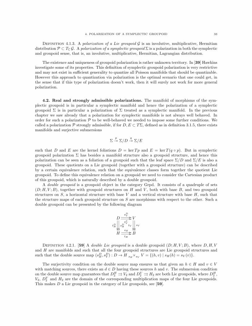
4. POLARIZATION OF A SYMPLECTIC GROUPOID 33
Definition 4.1.3. A polarization of a Lie groupoid G is an involutive, multiplicative, Hermitiandistribution P ⊂ TC G. A polarization of a symplectic groupoid Σ is a polarization in both the symplecticand groupoid sense, that is, an involutive, multiplicative, Hermitian, Lagrangian distribution.
The existence and uniqueness of groupoid polarization is rather unknown territory. In [39] Hawkinsinvestigate some of its properties. This definition of symplectic groupoid polarization is very restrictiveand may not exist in sufficient generality to quantize all Poisson manifolds that should be quantizable.However this approach to quantization via polarization is the optimal scenario that one could get, inthe sense that if this type of polarization doesn’t work, then it will surely not work for more generalpolarization.
4.2. Real and strongly admissible polarizations. The manifold of morphisms of the sym-plectic groupoid is in particular a symplectic manifold and hence the polarization of a symplecticgroupoid Σ is in particular a polarization of Σ treated as a symplectic manifold. In the previouschapter we saw already that a polarization for symplectic manifolds is not always well behaved. Inorder for such a polarization P to be well-behaved we needed to impose some further conditions. Wecalled a polarization P strongly admissible, if for D,E ⊂ TΣ, defined as in definition 3.1.5, there existsmanifolds and surjective submersions
Σp Σ/D
q Σ/E
such that D and E are the kernel foliations D = kerTp and E = kerT (q p). But in symplecticgroupoid polarization Σ has besides a manifold structure also a groupoid structure, and hence thispolarization can be seen as a foliation of a groupoid such that the leaf space Σ/D and Σ/E is also agroupoid. These quotients on a Lie groupoid (together with a groupoid structure) can be describedby a certain equivalence relation, such that the equivalence classes form together the quotient Liegroupoid. To define this equivalence relation on a groupoid we need to consider the Cartesian productof this groupoid, which is naturally described by a double groupoid.
A double groupoid is a groupoid object in the category Grpd. It consists of a quadruple of sets(D;H,V ;B), together with groupoid structures on H and V , both with base B, and two groupoidstructures on S, a horizontal structure with base V and a vertical structure with base H, such thatthe structure maps of each groupoid structure on S are morphisms with respect to the other. Such adouble groupoid can be presented by the following diagram
DsDV //tSV
//
sDH
tDH
V
sV
tV
H
sH //tH// B
Definition 4.2.1. [59] A double Lie groupoid is a double groupoid (D;H,V ;B), where D,H, Vand H are manifolds and such that all the four groupoid structures are Lie groupoid structures andsuch that the double source map (sDH , s
DV ) : D → H ×sH sV V = (h, v) | sH(h) = sV (v).
The surjectivity condition on the double source map ensures us that given an h ∈ H and v ∈ Vwith matching sources, there exists an d ∈ D having these sources h and v. The submersion conditionon the double source map guarantees that DH
2 ⇒ V2 and DV2 ⇒ H2 are both Lie groupoids, where DH
2 ,V2, DV
2 and H2 are the domain of the corresponding multiplication maps of the four Lie groupoids.This makes D a Lie groupoid in the category of Lie groupoids, see [59].

34 3. GEOMETRIC QUANTIZATION OF POISSON MANIFOLDS
Example 4.2.2. Let G ⇒ M be a Lie groupoid. Then the pair groupoid of G is a double Liegroupoid Pair(G) := G ×G, which can be presented by the diagram
G ×G // //
G
M ×M //// M
A double Lie subgroupoid of a double Lie groupoid (D;H,V ;B) is a double Lie groupoid (D′;H ′, V ′;B′)such that D′ ⇒ H ′, D′ ⇒ V ′, H ′ ⇒ B′, V ′ ⇒ B′ are respectively Lie subgroupoids of D ⇒ H, D ⇒ V ,H ⇒ B, V ⇒ B.
Definition 4.2.3. A smooth congruence of a Lie groupoid G is a closed, embedded sub double Liegroupoid of Pair(G) that is wide over G.
Hence a smooth congruence on G consisting of a pair (S,R) can be described by the followingdiagram
S
R
⊆
⊆
G ×G // //
G
M ×M //// M
For any such smooth congruence (S,R) on a Lie groupoid G ⇒ M , there exist a unique Lie groupoidstructure on the the quotients sets G′ = G /S, M ′ = M/R, such that the natural projections F : G → G′,f : M →M ′ form a morphism of Lie groupoids. In fact (F, f) form a fibration.
Definition 4.2.4. A fibration of Lie groupoids is a morphism of Lie groupoids F : G → G′,f : M →M ′ such that the base map f and the map
(F, s) : G → G′ ×t f M = (g, x) | t(g) = f(x)
are surjective submersions.
In this way the smooth congruence (S,R) defines a quotient Lie groupoid G /S ⇒M/R such thatthe natural projections (F, f) from the Lie groupoid G ⇒M is a fibration. Conversely every fibrationF : G → G′, f : M →M ′ of Lie groupoids determines a smooth congruence (R(F ), R(f)) on G. Hencethe notion of a smooth congruence and fibration are equivalent, which is proven in detail in [41].
Definition 4.2.5. A real polarization (of a symplectic manifold, groupoid, or symplectic groupoid)is a real distribution P whose complexification PC is a polarization.
Remember any polarization that satisfies P = P is the complexification of a real polarization andhence we regard a real polarization as a special case of complex polarization.
A real polarization P ⊂ T G is in particular a foliation of G and we want that the leaf spaceof this foliation has beside a manifold structure also a groupoid structure. Now we first notice thatT G can be seen as a Lie algebroid-groupoid associated to a the double Lie groupoid Pair(G). A Liealgebroid-groupoid arises from a single application of the Lie functor to a double Lie groupoid.

4. POLARIZATION OF A SYMPLECTIC GROUPOID 35
Definition 4.2.6. [60] A Lie algebroid-groupoid is given by the following data
Ω
qΩ
ρΩ
!!
tΩ //sΩ
// AρA
""
qA
T G
πG~~
TtG //TsG
// TM
πMG
tG //sG
// M
where G is a Lie groupoid on M and A is a Lie algebroid on M , and where Ω has both a Lie algebroidstructure on base G and a Lie groupoid structure on base A, such that the structure maps of the Liegroupoid structure on Ω are Lie algebroid morphisms and such that the double source map (qΩ, sΩ) :Ω→ G ×qA sA A is a surjective submersion.
Now consider a double Lie groupoid (D;H,V,B) then we can apply the Lie functor A to thevertical groupoid structure on D and V to get a vertical Lie algebroid-groupoid
A(D)
qA(D)
ρA(D)
##
sA(D) //tA(D)
// A(V )ρA(V )
##
qA(V )
TH
πH
TsH //TtH
// TB
πB
HsH //tH
// B
Similarly we can apply the Lie functor A to the horizontal groupoid structure on D and H to get ahorizontal Lie algebroid-groupoid[60]
A(D)qA(D) //
ρA(D)
''sA(D)
tA(D)
V
sV
tV
TV
πV
88
TtV
TsV
A(H)qA(H) //
ρA(H)
''
B
TB
πB
88
Example 4.2.7. Let G be a Lie groupoid on M and consider the double Lie groupoid Pair(G) asin the example above. Then the vertical Lie algebroid-groupoid and horizontal Lie algebroid-groupoid
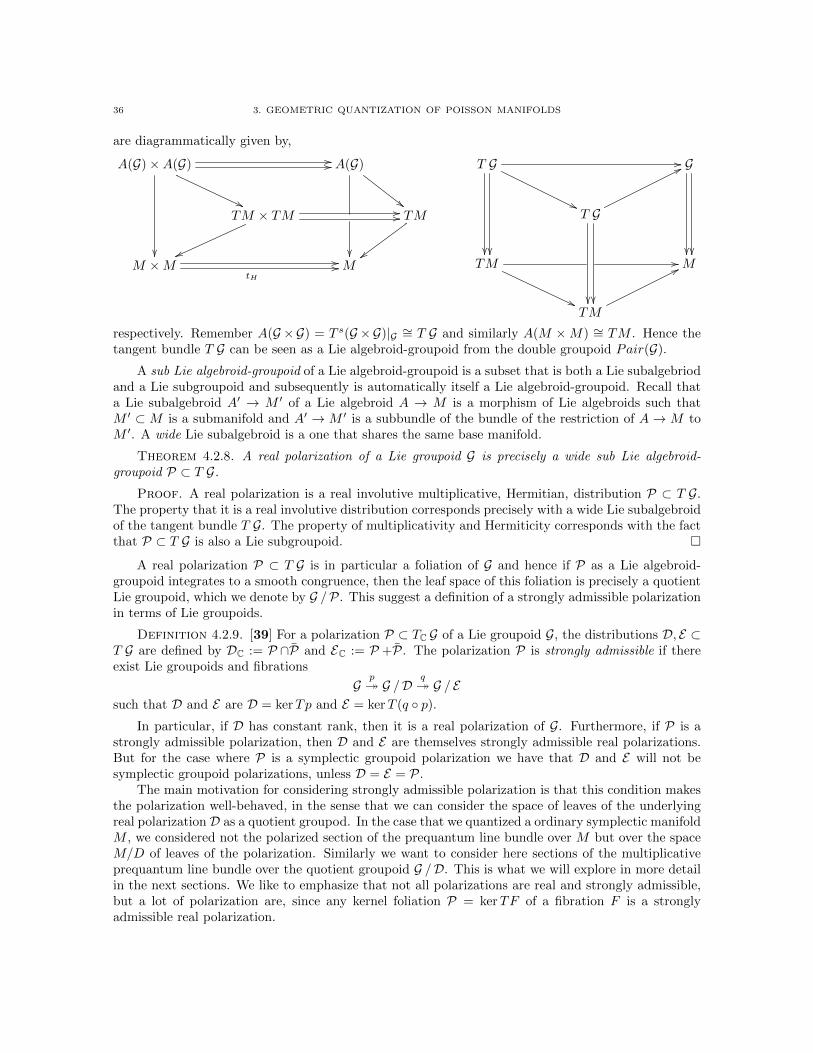
36 3. GEOMETRIC QUANTIZATION OF POISSON MANIFOLDS
are diagrammatically given by,
A(G)×A(G)
''
//// A(G)
##
TM × TM
vv
//// TM
M ×M //
tH// M
T G //
''
G
T G
77
TM //
''
M
TM
77
respectively. Remember A(G ×G) = T s(G ×G)|G ∼= T G and similarly A(M ×M) ∼= TM . Hence thetangent bundle T G can be seen as a Lie algebroid-groupoid from the double groupoid Pair(G).
A sub Lie algebroid-groupoid of a Lie algebroid-groupoid is a subset that is both a Lie subalgebriodand a Lie subgroupoid and subsequently is automatically itself a Lie algebroid-groupoid. Recall thata Lie subalgebroid A′ → M ′ of a Lie algebroid A → M is a morphism of Lie algebroids such thatM ′ ⊂ M is a submanifold and A′ → M ′ is a subbundle of the bundle of the restriction of A → M toM ′. A wide Lie subalgebroid is a one that shares the same base manifold.
Theorem 4.2.8. A real polarization of a Lie groupoid G is precisely a wide sub Lie algebroid-groupoid P ⊂ T G.
Proof. A real polarization is a real involutive multiplicative, Hermitian, distribution P ⊂ T G.The property that it is a real involutive distribution corresponds precisely with a wide Lie subalgebroidof the tangent bundle T G. The property of multiplicativity and Hermiticity corresponds with the factthat P ⊂ T G is also a Lie subgroupoid.
A real polarization P ⊂ T G is in particular a foliation of G and hence if P as a Lie algebroid-groupoid integrates to a smooth congruence, then the leaf space of this foliation is precisely a quotientLie groupoid, which we denote by G /P. This suggest a definition of a strongly admissible polarizationin terms of Lie groupoids.
Definition 4.2.9. [39] For a polarization P ⊂ TC G of a Lie groupoid G, the distributions D, E ⊂T G are defined by DC := P ∩P and EC := P +P. The polarization P is strongly admissible if thereexist Lie groupoids and fibrations
Gp G /D
q G / E
such that D and E are D = kerTp and E = kerT (q p).In particular, if D has constant rank, then it is a real polarization of G. Furthermore, if P is a
strongly admissible polarization, then D and E are themselves strongly admissible real polarizations.But for the case where P is a symplectic groupoid polarization we have that D and E will not besymplectic groupoid polarizations, unless D = E = P.
The main motivation for considering strongly admissible polarization is that this condition makesthe polarization well-behaved, in the sense that we can consider the space of leaves of the underlyingreal polarization D as a quotient groupod. In the case that we quantized a ordinary symplectic manifoldM , we considered not the polarized section of the prequantum line bundle over M but over the spaceM/D of leaves of the polarization. Similarly we want to consider here sections of the multiplicativeprequantum line bundle over the quotient groupoid G /D. This is what we will explore in more detailin the next sections. We like to emphasize that not all polarizations are real and strongly admissible,but a lot of polarization are, since any kernel foliation P = kerTF of a fibration F is a stronglyadmissible real polarization.

5. TWISTED POLARIZED CONVOLUTION ALGEBRA 37
5. Twisted polarized convolution algebra
In section 3 we constructed a twisted convolution algebra of a general Lie groupoid G, using half-densities. The convolution algebra was defined for certain sections of the half-density bundle Ω1/2 overG and the twisted convolution algebra was defined for certain section of the bundle L ⊗ Ω1/2 whereL was the Hermitian line bundle of the twist of the Lie groupoid. In the presence of a strongly ad-missible polarization of G, we can restrict this to sections that are polarized, which we will turn to now.
Let G be a Lie groupoid and P ⊂ T G a strongly admissible real polarization of G. Then we havethat P is the kernel foliation of the fibration
p : G → G /P
Instead of considering the convolution algebra of G we want to consider the convolution algebra of thequotient Lie groupoid G /P. In [39] Hawkins defines the polarized convolution algebra of any stronglyadmissible real polarization as the convolution algebra
C∗P(G) := C∗(G /P)
An element of this polarized convolution algebra is a section of the half-density bundle Ω1/2 over G /P,which should correspond to a polarized section of p∗Ω1/2. Remember that the half-density bundle onG /P was defined by Ω1/2 = |Ω|1/2(∧max(T t∗C (G /P)⊕T s∗C (G /P))). The pullback of this bundle alongp gives
p∗Ω1/2 ∼= Ω1/2P := |Ω|1/2(∧max(T t G /(T t G ∩P)⊕ T s G /(T s G ∩P))∗C)
Where we used that p∗T t(G /P) ∼= T t G /(T t G ∩P) and p∗T s(G /P) ∼= T s G /(T s G ∩P). Similarly tothe result in section 3 we have that
pr∗1Ω1/2P ⊗ pr∗2Ω
1/2P∼= m∗Ω
1/2P ⊗ pr∗1 |Ω|1(∧max(T t G /(T t G ∩P))∗C)
where on the left we tensor with the pullback pr1∗ of the bundle of volume forms along the t-fibers that
are transverse to P. Hence for two global polarized sections f, g ∈ Γ(G,Ω1/2P ), meaning the pullbacks of
sections over G /P, that are compactly supported modulo P, the polarized convolution can be definedsimilarly to the integral of definition 3.1.2, only we do not integrate over the fiber t−1(t(γ)) but overthe quotient space, since the integrand is constant along P-fibers.
We can extend this definition of Ω1/2P to an arbitrary strongly admissible polarization P, by defining
the half-density bundle as
Ω1/2P := |Ω|1/2(∧max(T tC G /(T tC G ∩P)⊕ T sC G /(T sC G ∩P))∗)
provided that T t G ∩P has constant rank. If it does not have constant rank then T t G ∩P is not a
bundle, and hence Ω1/2P is not defined. Furthermore we require that Ω
1/2P satisfies
i∗Ω1/2P∼= Ω
1/2P
where i is the groupoid inverse.
Remark 5.0.10. This half-density bundle Ω1/2P may not be unique, since there is a choice of square
root involved. Any other choice is obtained by tensoring the bundle Ω1/2P with a real line bundle which
is isomorphic to its pullback by the groupoid inverse (see [39]).
This half-density bundle Ω1/2P also carries a natural flat P-connection and our previous definition,
for the case of a strongly admissible real polarization, of polarized section as the pullback by p of asection of G /P can be expressed in terms of this connection. Due to Hawkins we have the following
38 3. GEOMETRIC QUANTIZATION OF POISSON MANIFOLDS
Theorem 5.0.11. [39] If P is a polarization of a Lie groupoid G, then the P-Bott connection
induces a natural flat P-connection ∇ on Ω1/2P whenever this bundle is defined.
With this connection we can speak of polarized sections of Ω1/2P in the ordinary sense, that is
if U ⊂ G is an open subset, then f ∈ Γ(U,Ω1/2P ) is polarized if ∇Xf = 0 for any X ∈ Γ(U,P).
This definition recovers our previous definition in terms of pullback and extends to arbitrary stronglyadmissible polarizations.
However, for arbitrary strongly admissible polarizations there is a pitfall in defining the polarizedconvolution of two polarized sections, since we do not have in general that P = D = E , as in the real
case. For two polarized sections f, g ∈ Γ(U,Ω1/2P ) the polarized convolution should be defined by some
integral over the integrand of definition 3.1.2
f(η)g(η−1γ)
where η ∈ t−1(t(γ)). Since the sections f and g are polarized, the integrand is covariantly constantalong the foliation D restricted to t−1(t(γ)), and hence we should integrate over the quotient by D,instead of the quotient by P as in the real case. In order to integrate over the quotient one would liketo have an isomorphism
pr∗1Ω1/2P ⊗ pr∗2Ω
1/2P∼= m∗Ω
1/2P ⊗ pr∗1 |Ω|1(∧max(T t G /(T t G ∩D))∗C)
Instead one has the natural isomorphism[39]
pr∗1Ω1/2P ⊗ pr∗2Ω
1/2P∼= m∗Ω
1/2P ⊗ pr∗1 |Ω|1(∧max(T t G /(T t G ∩D))∗C)⊗ pr∗1 |Ω|1(∧max(T t G /(T t G ∩E))∗C)
This may not always reduce to the isomorphism we would like to have, but in the case that we have asymplectic structure on the Lie groupoid it does reduce, by the following result.
Theorem 5.0.12. [39] If P is a polarization of a symplectic groupoid Σ and T tCΣ∩P has a constant
rank, then for some k ∈ N the contraction with ωk
k! gives an isomorphism
∧max(T tΣ ∩ E)∼→ ∧max(T tΣ ∩ D)
This isomorphism will induce the isomorphism
pr∗1Ω1/2P ⊗ pr∗2Ω
1/2P∼= m∗Ω
1/2P ⊗ pr∗1 |Ω|1(∧max(T tΣ/(T tΣ ∩ D))∗C)
which would make the integration meaningful.However in order to define the polarized convolution on the symplectic groupoid, we need to have
suitable global polarized sections, which in general may not exist, this is illustrated by the followingexample.
Example 5.0.13. Consider the pair groupoid Pair(T2) of the complex torus T2 where we takethe reversed complex structure on the second factor. Take for the polarization the antiholomorphictangent bundle, that is P = T0,1T2⊕T1,0T2 ⊂ TCPair(T2). Explicitly we have T tCPair(T2) = TCT2⊕0and T sCPair(T2) = 0⊕TCT2 and hence T tCPair(T2)∩P = T0,1T2⊕0 and T sCPair(T2)∩P = 0⊕T1,0T2,which gives
Ω1/2P = |Ω|1/2 ∧max (T1,0T2 ⊕ T0,1T2)∗
A global section of this bundle is equivalent to a holomorphic function on T4. By an implication ofLiouville’s theorem, there are no non-constant global section of a holomorphic functions on a compact
complex manifold, hence every global sections of Ω1/2P has to be a constant, which implies that Ω
1/2P is
the trivial bundle. Thus global polarized sections of Ω1/2P are not suitable for defining a convolution
algebra. However if Ω1/2P is twisted by a line bundle with positive curvature, there will exist many
suitable holomorphic sections[39].
6. REAL POLARIZATION AND BOHR-SOMMERFELD CONDITION 39
This lead to the twisted polarized convolution algebra, which we denote by C∗P(Σ, σ). Let P bea strongly admissible polarization of a symplectic groupoid Σ and (σ,L,∇) a prequantization. The
connection on L with the partial connection on Ω1/2P give together a flat P-connection on L ⊗ Ω
1/2P ,
which defines locally the polarized sections. In the definition 2.1.7 of a prequantization of Σ we addedthe compatibility condition of the connection ∇ with the twist σ. This compatibility condition wasneeded in order for
σ(η, η−1γ)f(η)g(η−1γ)
to be covariantly D-constant as a function of η ∈ t−1(t(γ)), where f, g ∈ Γ(Σ,L⊗ Ω1/2P ) are polarized
sections. The twisted convolution f ∗ g is now defined as the integration of σ(η, η−1γ)f(η)g(η−1γ) overthe quotient, whenever it make sense. The integration only make sense by choosing a suitable fall-offcondition. Remember that without a polarization the convolution algebra was defined with compactlysupported sections. For a strongly admissible polarization, compactly supported sections will onlyexist if the leaves of the foliation E are compact. In some cases a weaker fall-off condition may also besuitable for producing the same C∗-algebra, but a general prescription for this weaker fall-off conditionis still not at hand. Furthermore the space of polarized sections for a strongly admissible polarizationmay be too small in some cases. This may be resolved by taking the total sheaf cohomology of polarized
sections of L⊗Ω1/2P into account as is suggested by the idea of ”cohomological wave functions”, however
the lack of the inner product of cohomological wave functions has to be resolved first. In any case if Pis strongly admissible with Ω
1/2P a bundle such that the higher degree cohomology of polarized sections
of L⊗ Ω1/2P vanishes, then the convolution algebra should consist of global polarized sections[39].
6. Real polarization and Bohr-Sommerfeld condition
Let P be a strongly admissible real polarization of a symplectic groupoid Σ, with p : Σ → Σ/Pthe quotient fibration and let (σ,L,∇) be a prequantization of Σ. In the case that the leaves of P aresimply connected we have that the connection trivializes L along these leaves, which means that thereis a line bundle L0 over Σ/P such that L ∼= p∗L0. Since the line bundle L carries a twist σ the linebundle L0 carries also a twist σ0 such that
C∗P(Σ, σ) ∼= C∗(Σ/P, σ0)
This cocycle with coefficients in L0 we call the reduced cocycle. If furthermore the line bundle Lis trivializable, which happens in a lot of examples, then the connection can be given by a 1-formθ ∈ Ω1(Σ) as ∇ = d + iθ. There exists a particular interesting class of 1-forms which makes it veryeasy to compute the reduced cocycles for the corresponding prequantization.
Definition 6.0.14. [39] A symplectic potential is a 1-form θ ∈ Ω1(Σ) such that dθ = −ω and
1∗θ = 0. It is adapted if it is conormal to the polarization, i.e. θ ∈ Γ(Σ,P⊥).
Lemma 6.0.15. [39] Let P be a strongly admissible real polarization of a symplectic groupoid Σ,with p : Σ→ Σ/P the quotient fibration. If θ is an adapted symplectic potential, then L0 is trivial andthe reduced cocycle σ0 ∈ Γ([Σ/P]2, U(1)) is given (up to a locally constant phase) by
p∗(σ−10 dσ0) = i∂∗θ
Usually there exists a real function φ ∈ C∞([Σ/P]2) such that
dp∗φ = ∂∗θ
and σ0 = eiφ.
Remark 6.0.16. To compute the algebra up to isomorphism we only need the cohomology classof [σ0] ∈ Tw(Σ/P) such that Tw(p)[σ0] ' [σ].
40 3. GEOMETRIC QUANTIZATION OF POISSON MANIFOLDS
Similar to the situation encountered in the construction of a Hilbert space, if the leaves of thepolarizations are not simply connected, then L will typically have non-trivial holonomy around non-contractable loops in these leaves. In this case, there is an open set over which the smooth polarized
sections of L⊗ Ω1/2P must vanish. This leads to the following definition.
Definition 6.0.17. The Bohr-Sommerfeld subgroupoid ΣB−S ⊂ Σ is the set of points through
which L⊗ Ω1/2P has trivial holonomy. The reduced groupoid it the quotient ΣB−S/P.
More generally, if P is a strongly admissible polarization, that is not necessarily real, then the Bohr-Sommerfeld conditions come from holonomy around the leaves of D. We have also a Bohr-Sommerfeldsubgroupoid ΣB−S and a reduced groupoid ΣB−S/D.
7. C∗-algebra
The final step is to complete the twisted polarized convolution algebra C∗P(Σ, σ) to a C∗-algebra.This algebra is a generalization of the convolution algebra of a groupoid, and hence we expect thatthere will be more than one natural way of completing it. We explain here that we can construct boththe maximal and the reduced C∗-algebras from the twisted polarized convolution algebra, which mightgive a suitable quantization.
Assume from now on that the algebras are defined over the field C.
Definition 7.0.18. A Banach algebra is a Banach space (A, ‖‖) with an associative algebra struc-ture, such that for all x, y ∈ A one has: ‖xy‖ ≤ ‖x‖‖y‖.
A morphism of Banach algebras A and B is a bounded linear map φ : A → B satisfying φ(ab) =φ(a)φ(b).
Definition 7.0.19. Let A be an algebra. An involution on A is an antilinear operator ∗ : A → A(i.e. for x, y ∈ A, λ, µ ∈ C, one has (λx + µy)∗ = λx∗ + µy∗), such that for all x, y ∈ A, one has(xy)∗ = y∗x∗, and x∗∗ = x. An algebra equipped with an involution is called a ∗-algebra.
Definition 7.0.20. A C∗-algebra is a Banach algebra A with an involution ∗, such that for allx ∈ A, ‖x‖2 = ‖x∗x‖. This norm ‖‖ satisfying this condition is also called a C∗-norm.
A morphism of C∗-algebras A and B is a morphism of Banach algebras φ : A → B satisfyingφ(a∗) = φ(a)∗, which is also called a ∗-homomorphism.
Example 7.0.21. Suppose X is a locally compact Hausdorff space. The space C0(X) of continuousfunctions on X that vanish at infinity, form a commutative C∗-algebra under pointwise multiplicationof functions and involution given by f∗(x) := f(x). The norm is the supremum norm of functions(i.e. ‖f‖ = sup|f(x)| : x ∈ X). Conversely, it is known that if A is a commutative C∗-algebra thenthere is a locally compact Hausdorff space X, such that A is isometrically isomorphic to the algebraC0(X). In fact it can be shown that the correspondence X 7→ C(X) is a faithful contravariant functorfrom the category of compact Hausdorff spaces (with morphisms being continuous maps) to that ofcommutative C∗-algebras with unit.
Example 7.0.22. An example of noncommutative C∗-algebra is B(H), the algebra of boundedlinear operators on a Hilbert space H. The multiplication is given by composition, the involution isgiven by taking the the adjoint, and the norm is the operator norm (i.e. ‖P‖ := sup‖P (h)‖ : h ∈H, ‖h‖ = 1 for all P ∈ B(H)).
Definition 7.0.23. For A a ∗-algebra and H a Hilbert space, a ∗-representation of A on H is a∗-homomorphism π : A→ B(H). A ∗-representation π is said to be faithful if ker(π) = 0.
For A a C∗-algebra we call a ∗-representation of A just a representation.

8. EXAMPLES 41
Theorem 7.0.24. (The Gelfand-Naimark representation theorem) Any C∗-algebra has a faithfulrepresentation.
Example 7.0.25. SupposeH is a Hilbert space. For elements h, h′ ∈ H one can define the operatorh〈h′, .〉 : H → H. All the operators of this form generate a ∗-subalgebra of B(H). The norm-closure ofthis algebra is the C∗-algebra K(H) of compact operators. A given operator T ∈ B(H) is compact iffT maps the unit ball in H to a set with compact closure.
Let C∗P(Σ, σ) be the twisted polarized convolution algebra, which is in particular a ∗-algebra. Tomake it a C∗-algebra we need to define a C∗-norm on C∗P(Σ, σ). LetR be the set of all ∗-representationsπ for which π is continuous when C∗P(Σ, σ) has the inductive limit topology and B(H) the weak operatortopology and such that the linear span π(f)ξ : f ∈ C∗P(Σ, σ), ξ ∈ H is dense in H. One defines themaximal C∗-norm of f ∈ C∗P(Σ, σ) by [69]
‖f‖max := supπ∈R‖π(f)‖
Definition 7.0.26. The completion of C∗P(Σ, σ) with respect to the norm ‖‖max is the maximalC∗-algebra, which we denote also by C∗P(Σ, σ).
The reduced C∗-algebra should be defined using a (left) regular representation of the twistedpolarized convolution algebra C∗P(Σ, σ). Since P is a strongly admissible polarization of the symplecticgroupoid Σ we have a fibration p : Σ → Σ/D. For each point in the leaf in the base of Σ/D one hasa natural ∗-representation of the ∗-algebra. Fix a point x ∈ Σ0 such that p(x) ∈ (Σ/D)0, we define arepresentation πx of C∗P(Σ, σ) on the Hilbert space L2(s−1(x)∩Σ/D, σ) of square integrable (twisted)half-densities on the s-fiber of x intersected with Σ/D by
(πx(f)ξ)(γ) =
∫η∈t−1(t(γ))∩Σ/D
σ(η, η−1γ)f(η)ξ(η−1γ)
where f ∈ C∗P(Σ, σ) and ξ ∈ L2(s−1(x) ∩ Σ/D, σ). This representation is called a (left) regularrepresentation with respect to x, since πx(f)ξ(γ) = f ∗ ξ(γ).The inner-product on the Hilbert spaceL2(s−1(x) ∩ Σ/D, σ) is defined by
〈ξ, ξ〉 = ξ∗ ∗ ξ(x) =
∫y∈t−1(t(x))∩Σ/D
σ(y, y−1x)ξ∗(y)ξ(y−1x)
=
∫y∈s−1(x)∩Σ/D
σ(y−1, y)σ(y−1, y)ξ(y)ξ(y) <∞
Definition 7.0.27. [14] The completion of C∗P(Σ, σ) with respect to the norm ‖f‖red = supx∈Σ0‖πx(f)‖is
the reduced C∗-algebra, which we denote by C∗P(Σ, σ)red.
Hawkins studied several examples and it is not yet known which completion will fit a reasonabledefinition of quantization. Some examples in [39] suggest that both the maximal and reduced C∗-algebras are quantizations, some suggest that only the reduced C∗-algebra is a natural quantizationand the results in [43] suggests that the maximal C∗-algebra is most suitable.
8. Examples
At last we will give two examples to illustrate the above quantization procedure for Poisson man-ifolds, which can also be found in [39]. We will start with the motivating example where we considerthe quantization of symplectic manifold and show how we reproduce the C∗-algebra of compact opera-tors. The second example concerns the quantization of a linear Poisson manifold, and we will see howthis reproduce the usual Moyal quantization of Poisson vector spaces. For more examples we refer thereader to [39].

42 3. GEOMETRIC QUANTIZATION OF POISSON MANIFOLDS
8.1. Symplectic manifold. Let (M,ωM ) be a symplectic manifold with a polarization F ⊂ TCMand a prequantization (L, 〈, 〉,∇). Then we have the pair groupoid Σ := Pair(M) as the integratedsymplectic groupoid, with multiplicative symplectic form ω := t∗ωM−s∗ωM , as is explained in example1.0.23 of appendix A. The polarization F of M induces a symplectic groupoid polarization P := F ×Fon Pair(M). To see this we mention first that the set of composable pairs can be identified asΣ2∼= M × M × M and the multiplication map m : Σ2 → Σ simply forgets the middle factor.
Hence P2 = (P ×P) ∩ TCΣ2 = F ×(F ∩F) × F from which one sees that P is multiplicative andTi(P) = Ti(F ×F) = F × F = P implies that P is Hermitian, the fact that P is an involutiveLagrangian distribution is immediate and hence P is a symplectic groupoid polarization of Pair(M).In particular, if F is a real polarization of M , the polarization P = F ×F is just a pairs of vectorsfrom F where two such pairs are composable if the second of the first pair and the first of the secondpair coincide, that is P2 = F ×F ×F .
Example 8.1.1. (Vertical polarization) Let Q be a compact manifold, and M = T ∗Q be itscotangent bundle, with as polarization the vertical polarization which, as is explained in example3.1.7, is just the kernel foliation of the projection down to Q. Similarly the pair groupoid Pair(T ∗Q) ∼=T ∗(Pair(Q)) and hence the induced polarization P is just the kernel foliation of the projection downto Pair(Q), which is itself the reduced groupoid. As in example 3.1.7 one has also a tautological1-form θ = t∗τ − s∗τ on the cotangent bundle T ∗(Pair(Q)) which is a symplectic potential. Thissymplectic potential is adapted since for any element of the polarization P the form vanishes and it ismultiplicative, that is ∂∗θ = 0, since θ = ∂∗τ . But multiplicativity means that dp∗φ = 0 and hence wehave that σ0 = eiφ is locally constant from which can conclude that the reduced cocycle is trivial. Thisgives C∗P(Pair(T ∗Q), σ) ∼= C∗(Pair(Q), σ0), which is precisely equivalent to the untwisted groupoidconvolution algebra C∗(Pair(Q)). The completion of this to the reduced C∗-algebra is equivalentto the C∗-algebra of compact operators K(L2(Q)). For every x ∈ M one has that s−1(x) ∩ Σ/P ∼=T ∗Q⊕0∩Pair(Q) ∼= Q, which gives precisely the Hilbert space L2(Q) of square integrable half-densitieson Q. The (left) regular representation is given by
(πx(f)ξ)(γ) =
∫η∈Q
f(η)ξ(η−1γ)
=
∫η1∈Q
f(η1η−12 )ξ(η2)
where f ∈ C∗P(Pair(T ∗Q), σ) and ξ ∈ L2(Q). But if we define k(η1, η2) = f(η1η−12 ) for every η1, η2 ∈
Q, then it is immediate that k is the smoothing kernel of the operator πx(f) with a finite L2-norm andhence πx(f) defines a compact operator on L2(Q)[14]. Which gives the expected quantization[39]
C∗P(Pair(T ∗Q), σ) ∼= K(L2(Q))
Example 8.1.2. (Kahler polarization) Let (M,J, ω) be a compact Kahler manifold together withthe antiholomorphic tangent bundle F := T0,1M as the natural Kahler polarization, as in example3.1.4. The induced polarization P := F ×F on Pair(M) is just a pair of vectors, where two suchpairs are composable if the second of the first and the first of the second pair both vanish, that isP2 = F ×0 × F . This polarization P of Pair(M) is equivalent to a Kahler structrure on Pair(M)itself. For a prequantization (L, 〈, 〉,∇) on M we had that the polarized sections of L are precisely theholomorphic sections. Similarly one finds that the convolution product between polarized sections ofthe line bundle over Pair(M) is precisely the convolution product between holomorphic sections ofthis line bundle.
More generally, let M be a (compact) symplectic manifold with polarization F and prequantization(L, 〈, 〉,∇). We have Σ := Pair(M) and the symplectic groupoid polarization P := F ×F . In the
case that P is strongly admissible we can construct the half-density bundle Ω1/2P . First note that
8. EXAMPLES 43
T tCΣ = kerTCt = 0× TCM = s∗TCM and T tCΣ ∩ P = 0× F = s∗F , and hence
T tCΣ/(T tCΣ ∩ P) = s∗(TCM/F) = s∗(F⊥)∗
Remember F⊥ := ξ ∈ T ∗M : ∀X ∈ F , 〈X, ξ〉 = 0. Similarly we find
T sCΣ/(T sCΣ ∩ P) = t∗(F⊥)∗
which gives
Ω1/2P = |Ω|1/2(∧max(T tCΣ/(T tCΣ ∩ P)⊕ T sCΣ/(T sCΣ ∩ P))∗)
= |Ω|1/2 ∧max (t∗ F⊥⊕s∗F⊥)
= |Ω|1/2 ∧max (t∗ F⊥)⊗ |Ω|1/2 ∧max (s∗F⊥)
For the prequantization of Σ we consider the line bundle ∂∗L = t∗L ⊗ s∗L together with a twistσ. Then the algebra C∗P(Σ, σ) is constructed from the polarized sections of
t∗(L⊗ |Ω|1/2 ∧max F⊥)⊗ s∗(L⊗ |Ω|1/2 ∧max F⊥)
This space of polarized sections over Σ = M ×M is just a tensor product of the space of polarizedsections of L ⊗ |Ω|1/2 ∧max F⊥ over M with its complex conjugate. The completion of this twistedpolarized convolution algebra C∗P(Σ, σ) to the reduced C∗-algebra is equivalent to the C∗-algebra ofcompact operators K(L2(M/F , σ)). For every x ∈ M one has that s−1(x) ∩ Σ/P ∼= M ⊕ 0 ∩ (M ×M)/(F ×F) ∼= M/F , which gives precisely the Hilbert space L2(M/F , σ) of twisted square integrablehalf-densities on M/F . The (left) regular representation is given by
(πx(f)ξ)(γ) =
∫η∈M/F
σ(η, η−1γ)f(η)ξ(η−1γ)
where f ∈ C∗P(Σ, σ) and ξ ∈ L2(M/F , σ). These operators precisely form the algebra of boundedsmoothing kernels on M/F [14]. This algebra can be completed to the C∗-algebra K(L2(M/F , σ))of compact operators[39]. This example shows that Hawkins’ strict C∗-deformation quantizationrecovers the standard geometric quantization of symplectic manifolds, which in this particular casegives explicitly the Hilbert space of square integrable sections. From the physics perspective we havein well-behaved cases that, the Hilbert space L2(M/F , σ) is densely spanned by polarized sections
of L ⊗ |Ω|1/2 ∧max F⊥. The algebra K(L2(M/F , σ)) is densely spanned by the tensor product overPair(M) of a section and a complex conjugate section, which in physics is denoted by ”ket-bras”.But not all cases are well-behaved and the issues that one must be consider in constructing the innerproduct over M translates into issues in the construction of the convolution product over the groupoidΣ[39].
8.2. Poisson vector space with constant Poisson bivector. Here we consider a first non-trivial example of the strict C∗-deformation quantization. Let our Poisson manifold be a vector spaceV with a constant Poisson bivector π ∈ ∧2V . The cotangent bundle T ∗V is turned into a Lie algebroidas discussed in appendix A. This Lie algebroid can be integrated to the the symplectic groupoidΣ = T ∗V ∼= V ⊕ V ∗, where all the structure maps are linear. To see this let xi be coordinateson V and yi coordinates on V ∗, and let the symplectic 2-form ω in these coordinates be given byω = dxi ∧ dpi. The groupoid structure on Σ depends on the constant Poisson bivector π, which inthese coordinates is just a matrix (πij) and can be regarded as a map π : V ∗ → V . The inclusion mapof i : V → Σ is given by i(x) : (xi) 7→ (xi, pi). A morphism of γ ∈ Σ is given by a pair (xi, pi) and canbe described using Bopp shifts
xi − 12π
ijpj
γ++xi + 1
2πijpj
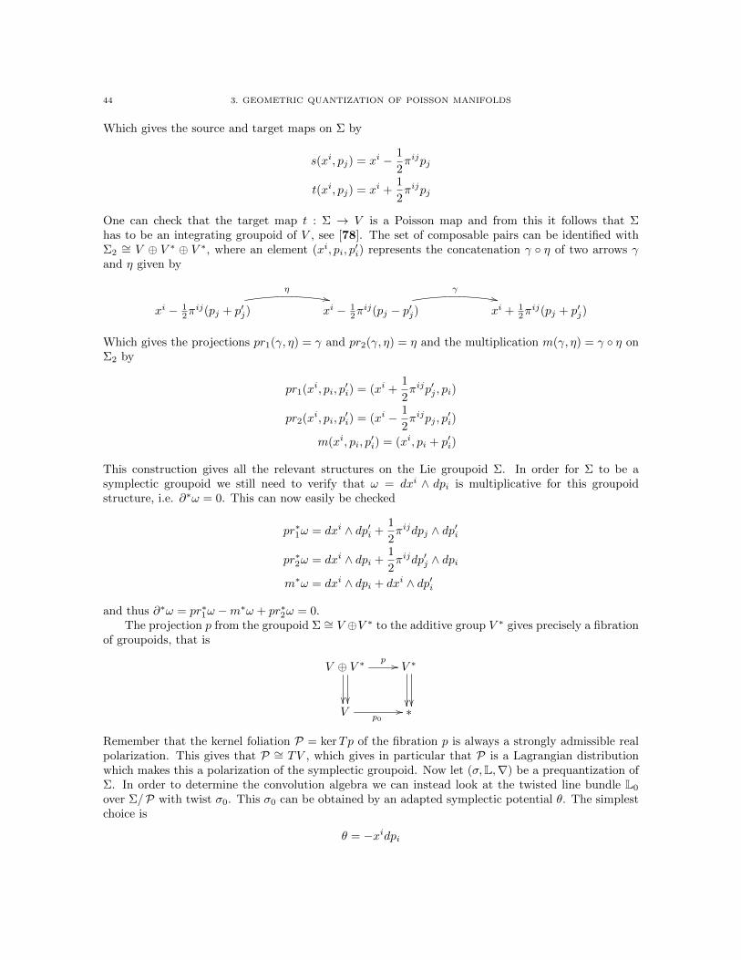
44 3. GEOMETRIC QUANTIZATION OF POISSON MANIFOLDS
Which gives the source and target maps on Σ by
s(xi, pj) = xi − 1
2πijpj
t(xi, pj) = xi +1
2πijpj
One can check that the target map t : Σ → V is a Poisson map and from this it follows that Σhas to be an integrating groupoid of V , see [78]. The set of composable pairs can be identified withΣ2∼= V ⊕ V ∗ ⊕ V ∗, where an element (xi, pi, p
′i) represents the concatenation γ η of two arrows γ
and η given by
xi − 12π
ij(pj + p′j)
η,,xi − 1
2πij(pj − p′j)
γ,,xi + 1
2πij(pj + p′j)
Which gives the projections pr1(γ, η) = γ and pr2(γ, η) = η and the multiplication m(γ, η) = γ η onΣ2 by
pr1(xi, pi, p′i) = (xi +
1
2πijp′j , pi)
pr2(xi, pi, p′i) = (xi − 1
2πijpj , p
′i)
m(xi, pi, p′i) = (xi, pi + p′i)
This construction gives all the relevant structures on the Lie groupoid Σ. In order for Σ to be asymplectic groupoid we still need to verify that ω = dxi ∧ dpi is multiplicative for this groupoidstructure, i.e. ∂∗ω = 0. This can now easily be checked
pr∗1ω = dxi ∧ dp′i +1
2πijdpj ∧ dp′i
pr∗2ω = dxi ∧ dpi +1
2πijdp′j ∧ dpi
m∗ω = dxi ∧ dpi + dxi ∧ dp′i
and thus ∂∗ω = pr∗1ω −m∗ω + pr∗2ω = 0.The projection p from the groupoid Σ ∼= V ⊕V ∗ to the additive group V ∗ gives precisely a fibration
of groupoids, that is
V ⊕ V ∗
p // V ∗
V
p0
// ∗
Remember that the kernel foliation P = kerTp of the fibration p is always a strongly admissible realpolarization. This gives that P ∼= TV , which gives in particular that P is a Lagrangian distributionwhich makes this a polarization of the symplectic groupoid. Now let (σ,L,∇) be a prequantization ofΣ. In order to determine the convolution algebra we can instead look at the twisted line bundle L0
over Σ/P with twist σ0. This σ0 can be obtained by an adapted symplectic potential θ. The simplestchoice is
θ = −xidpi

8. EXAMPLES 45
This symplectic potential is adapted since it is perpendicular to the polarization P. The twist σ0 canbe obtained by computing
∂∗θ = (xi +1
2πijp′j)dpi − xi(dpi + dp′i) + (xi − 1
2πijpj)dp
′i
= −1
2πijp′jdpi −
1
2πijpidp
′j
= d(−1
2πijpip
′j)
Hence
dp∗φ = d(−1
2πijpip
′j)
implies precisely that the reduced group cocycle σ0 : V ∗×V ∗ → U(1) is given by σ0(p, p′) = e−i2π(p,p′).
Alltogether, the twisted polarized convolution algebra C∗P(Σ, σ) is equivalent to the twisted convolutionalgebra C∗(V ∗, σ0), which is determined by the convolution product
(f ∗ g)(p) =
∫p′∈V ∗
e−i2π(p′,p−p′)f(p′)g(p− p′)
for functions f, g on V ∗, which is precisely the Moyal ?-product, which is usually written as a powerseries expansion of the exponential. The strict C∗-deformation quantization procedure of the Poissonvector space (V, π) gives precisely the twisted group algebra C∗(V ∗, σ0) and hence reproduces thefamous Moyal quantization of Poisson vector spaces, see [39, 72].


CHAPTER 4
Higher geometric perspective
Traditional geometric quantization applies to symplectic manifolds and not to Poisson manifolds.We saw in the previous chapter that there is a similar geometric quantization route via polarization forPoisson manifolds. Both geometric quantization procedures constructed a prequantum bundle. Overthe symplectic manifold we constructed a prequantum circle bundle and over the symplectic groupoidwe constructed a multiplicative prequantum circle bundle, which is a higher analog of a circle bundlewith connection and can be interpreted as a circle 2-bundle with connection. This is an instance ofhigher geometric prequantization, where the notion of prequantum circle bundle is refined to that of aprequantum circle n-bundle with connection for all n ∈ N.
To motivate higher geometric prequantization, it is helpful to look first at one of the fundamentalexamples of quantum field theory which is the 3-dimensional Chern-Simons theory as introduced in[92]. We will give a short review in the perpsective of higher stacks and treat the basic constructionsin classical Chern-Simons theory. This will give a blueprint along which we will interpreted theprequantization of the symplectic groupoid in terms of higher stacks. At the same time, this stackyperspective of the prequantization of a symplectic groupoid shows how it can be interpreted in highersymplectic geometry. This makes the geometric quantization of symplectic groupoids a good test caseagainst which to check notions of higher geometric quantization.
It turns out that the geometric prequantization of a Poisson manifold can be seen as the geometricprequantization of the 2d Chern-Simons theory, which here specifically is the case induced by a non-degenerate binary invariant polynomial, namely the Lie integrated version of the Poisson σ-model.This statement that there should be such a relation was already contained in Cattaneo and Felder[8], which identified the construction by Kontsevich of the algebraic deformation quantization of anyPoisson manifold, with the limiting case of the 3-point function in the perturbative quantization ofthe corresponding 2d Poisson σ-model. But at that time the geometric quantization of symplecticgroupoids as in [39] had yet to be fully understood. This shows that the geometric prequantization ofa Poisson manifold can be seen as the boundary of the Poisson σ-model.
The higher geometric quantization of a 2d field theory yields a 2-vector space of quantum 2-states.We will see that the 2-basis of this space of quantum 2-states is, up to Morita equivalence, an algebra.This algebra is precisely the algebra produced via strict C∗-deformation quantization by Hawkins.In the case that the Poisson manifold is a symplectic manifold, this algebra was the C∗-algebra ofcompact operators. But the C∗-algebra of compact operators are Morita equivalent to the groundfield, which precisely reflects the fact that in higher geometry Lie groupoids are considered up toMorita equivalence and that the pair groupoid is Morita equivalent to the point. This shows thatHawkins’ strict C∗-deformation quantization is not Morita faithful, in the sense that it distinguishMorita equivalent Lie groupoids and Mortia equivalent algebras.
1. Motivating examples
1.1. 3d Chern-Simons theory. To motivate higher geometric prequantization, it is helpful tolook first at one of the fundamental examples of quantum field theory which is the 3-dimensionalChern-Simons theory as introduced in [92]. See [23] for a comprehensive account and [29] for a higher
47

48 4. HIGHER GEOMETRIC PERSPECTIVE
stacky perspective. The reader who is uncomfortable reading this section, may read first section 2about smooth higher stacks.
First consider a compact connected and simply connected simple Lie group G and a 3-dimensionalsmooth (paracompact) manifold Σ3. Then there exist a classifying space BG, such that gauge equiv-alence classes of principal G-bundles over Σ3 are in natural bijective correspondence with the setH(Σ3, BG) of homotopy classes of maps from Σ3 to BG. Since BG is homotopically trivial in degreeless or equal to 3, any principal G-bundle on Σ3 can be trivialized. Now similarly write H(Σ3,BGconn)for the set of gauge equivalence classes of principal G-bundles with connection on Σ3. Since any prin-cipal G-bundle on Σ3 can be trivialized, for any gauge equivalence class of connections there existsa representative, which is given by a smooth g-valued 1-form A on Σ3. The action functional of 3dChern-Simons theory over Σ3 is a function of sets
exp(iS(−)) : H(Σ3,BGconn)→ U(1)
A 7→ exp(2πi
∫Σ3
CS(A))
Where CS(A) ∈ Ω3(Σ3) is the Chern-Simons 3-form of A, where CS is called the Lagrangian of thetheory. This action functional is well-defined since for every gauge transformation g : A → Ag forg ∈ C∞(Σ3, G) both A and its gauge transform Ag are mapped to the same element of U(1).
There are two important properties that is not immediatly seen from this action functional interms of sets. It has the property of being invariant under gauge transformation and it has theproperty of being smooth. A natural way to express the gauge invariance is to consider the groupoidH(Σ3,BGconn), whose objects are gauge fields A and whose morphisms are gauge transformations gas above. The gauge invariance of the action functional can then be expressed by functoriality, thatis by a morphism of groupoids exp(iS(−)) : H(Σ3,BGconn)→ U(1), where here U(1) is regarded as agroupoid with only identity morphisms. Furthermore the property of being smooth can be formulatedin terms of stacks, which we will explain in the next section in more detail. A stack on the site ofCartesian spaces maps to every Cartesian space U a groupoid, as above, of smooth U -families of gaugefields and a smooth U -family of gauge transformations between, in a consistent way. We will denotethe groupoid H(Σ3,BGconn) as a smooth stack by the same symbol and call it the smooth modulistack of gauge fields on Σ3. In fact Σ3 and BGconn can both be interpreted as stacks. Alltogether theChern-Simons action functional refines to a morphism of smooth stacks
exp(iS(−)) : H(Σ3,BGconn)→ U(1)
Where the groupoid U(1) is here regarded as a smooth stack. This refined action functional makes itexplicit that Chern-Simons theory is actually a gauge theory.
Remark 1.1.1. In the literature one usually distinguish between ”external hom” and ”internalhom”. Where one use the external hom for denoting H(Σ3,BGconn) as a groupoid and where one usethe internal hom , which is denoted by [Σ,BGconn], for the actual stack of fields. This stack is definedby the assignment
[Σ,BGconn] : U 7→ H(Σ× U,BGconn)
We will for simplicity not distinguish between these notations and we will use throughout this thesisonly the notation for the external hom. From the context it should be clear whether one needs tointerpreted it is a external or internal hom.
The smooth structure on the action functional allows us to define the differential d exp(iS(−)) of theaction functional and hence its critical locus, which is characterized by the Euler-Lagrange equationsof motion. In Chern-Simons theory this critical locus happens to be H(Σ3, [BG) the groupoid of
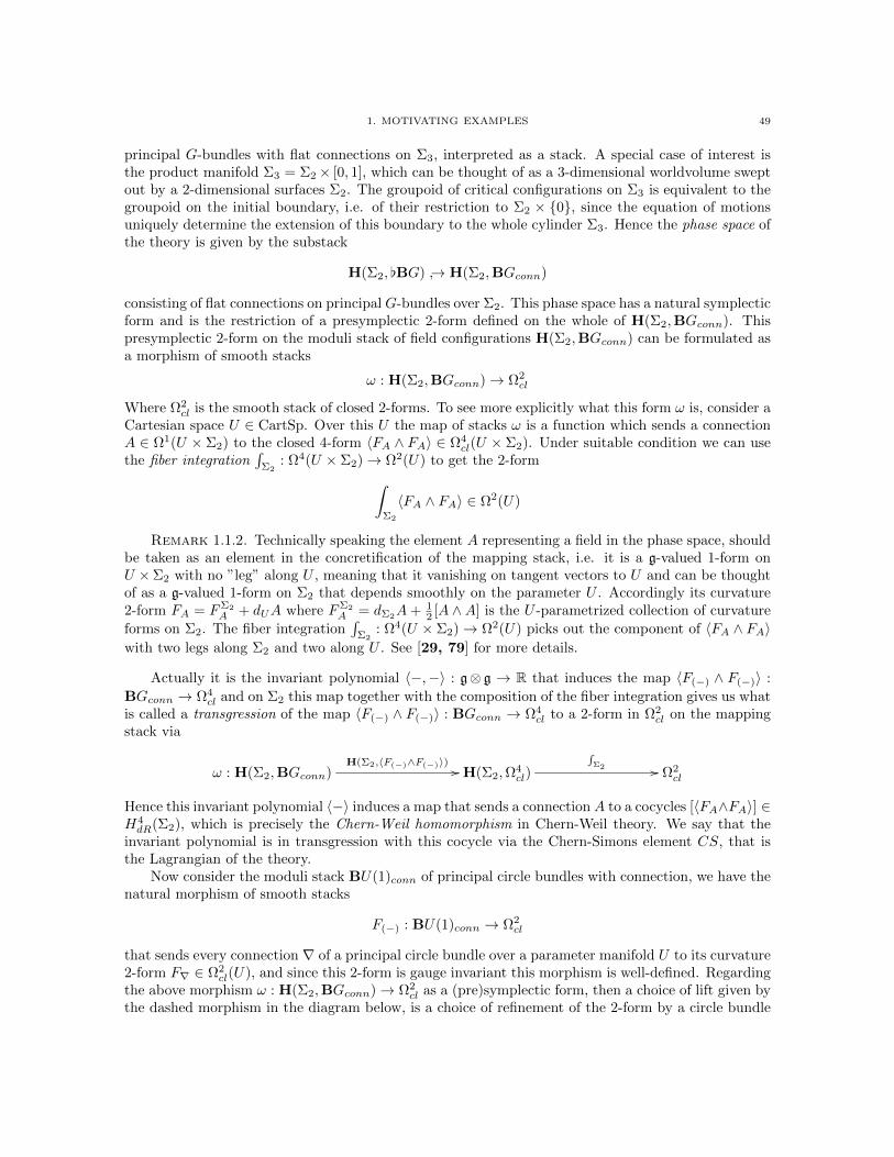
1. MOTIVATING EXAMPLES 49
principal G-bundles with flat connections on Σ3, interpreted as a stack. A special case of interest isthe product manifold Σ3 = Σ2× [0, 1], which can be thought of as a 3-dimensional worldvolume sweptout by a 2-dimensional surfaces Σ2. The groupoid of critical configurations on Σ3 is equivalent to thegroupoid on the initial boundary, i.e. of their restriction to Σ2 × 0, since the equation of motionsuniquely determine the extension of this boundary to the whole cylinder Σ3. Hence the phase space ofthe theory is given by the substack
H(Σ2, [BG) → H(Σ2,BGconn)
consisting of flat connections on principal G-bundles over Σ2. This phase space has a natural symplecticform and is the restriction of a presymplectic 2-form defined on the whole of H(Σ2,BGconn). Thispresymplectic 2-form on the moduli stack of field configurations H(Σ2,BGconn) can be formulated asa morphism of smooth stacks
ω : H(Σ2,BGconn)→ Ω2cl
Where Ω2cl is the smooth stack of closed 2-forms. To see more explicitly what this form ω is, consider a
Cartesian space U ∈ CartSp. Over this U the map of stacks ω is a function which sends a connectionA ∈ Ω1(U × Σ2) to the closed 4-form 〈FA ∧ FA〉 ∈ Ω4
cl(U × Σ2). Under suitable condition we can usethe fiber integration
∫Σ2
: Ω4(U × Σ2)→ Ω2(U) to get the 2-form∫Σ2
〈FA ∧ FA〉 ∈ Ω2(U)
Remark 1.1.2. Technically speaking the element A representing a field in the phase space, shouldbe taken as an element in the concretification of the mapping stack, i.e. it is a g-valued 1-form onU ×Σ2 with no ”leg” along U , meaning that it vanishing on tangent vectors to U and can be thoughtof as a g-valued 1-form on Σ2 that depends smoothly on the parameter U . Accordingly its curvature2-form FA = FΣ2
A + dUA where FΣ2
A = dΣ2A+ 1
2 [A ∧A] is the U -parametrized collection of curvature
forms on Σ2. The fiber integration∫
Σ2: Ω4(U × Σ2)→ Ω2(U) picks out the component of 〈FA ∧ FA〉
with two legs along Σ2 and two along U . See [29, 79] for more details.
Actually it is the invariant polynomial 〈−,−〉 : g⊗ g → R that induces the map 〈F(−) ∧ F(−)〉 :
BGconn → Ω4cl and on Σ2 this map together with the composition of the fiber integration gives us what
is called a transgression of the map 〈F(−) ∧ F(−)〉 : BGconn → Ω4cl to a 2-form in Ω2
cl on the mappingstack via
ω : H(Σ2,BGconn)H(Σ2,〈F(−)∧F(−)〉) // H(Σ2,Ω
4cl)
∫Σ2 // Ω2
cl
Hence this invariant polynomial 〈−〉 induces a map that sends a connection A to a cocycles [〈FA∧FA〉] ∈H4dR(Σ2), which is precisely the Chern-Weil homomorphism in Chern-Weil theory. We say that the
invariant polynomial is in transgression with this cocycle via the Chern-Simons element CS, that isthe Lagrangian of the theory.
Now consider the moduli stack BU(1)conn of principal circle bundles with connection, we have thenatural morphism of smooth stacks
F(−) : BU(1)conn → Ω2cl
that sends every connection ∇ of a principal circle bundle over a parameter manifold U to its curvature2-form F∇ ∈ Ω2
cl(U), and since this 2-form is gauge invariant this morphism is well-defined. Regardingthe above morphism ω : H(Σ2,BGconn)→ Ω2
cl as a (pre)symplectic form, then a choice of lift given bythe dashed morphism in the diagram below, is a choice of refinement of the 2-form by a circle bundle

50 4. HIGHER GEOMETRIC PERSPECTIVE
with connection and hence the choice of a prequantum circle bundle in the language of prequantization.
BU(1)conn
F(−)
H(Σ2,BGconn)
66
ω// Ω2cl
In summary we have the following table
dimension description moduli stackk = 3 action functional H(Σ3,BGconn)→ U(1)k = 2 prequantum circe bundle H(Σ2,BGconn)→ BU(1)conn
In dimension k the Chern-Simons theory appears as a circle (3−k)-bundle with connection at leastfor k = 2, 3. Indeed for the case k = 3, the action functional can be interpreted as a circle 0-bundlewith connection and for the case k = 2 the prequantum circle bundle is precisely a circle 1-bundle withconnection. In ordinary geometric quantization of Chern-Simons theory we construct a vector spacefrom this prequantum circle bundle over a closed manifold Σ2 by considering the polarized sections(holomorphic sections) of the line bundle associated to the this circle 1-bundle on Σ2. Hence this givesan assignment of a vector space to a closed manifold Σ2. According to the definition of a extendedtopological quantum field theory of dimension n, due to Lurie in [55], we can roughly assign a (n−k)-categorical analog of a vector space of quantum states to every closed k dimensional manifold afterquantization. Interpreting 3d Chern-Simons theory as an extended topological quantum field theorysuggests that for every closed oriented manifold of dimension 0 ≤ k ≤ 3 we can assigns a prequantumcircle (3− k)-bundle on the moduli stack of field configuration over Σk, that is a morphism
H(Σk,BGconn)→ B(3−k)U(1)conn
In particular for the case k = 0, we can take Σ0 the space ∗ consisting of a single point together withthe fact that H(∗,BGconn) ' BGconn, the geometric prequantization of the morphism 〈F(−) ∧ F(−)〉 :
BGconn → Ω4cl is a choice of refinement of the 4-form given by the dashed morphism
B3U(1)conn
BGconn
c
88
〈F(−)∧F(−)〉// Ω4cl
The vertical arrow is the higher analog of the curvature morphism and c is called the universal charac-teristic morphism and we call it also the extended Lagrangian. This morphism of smooth higher stacksis the differential refinement of a smooth refinement of the topological characteristic map, which de-termine what is called the level of the theory. By forgetting the connections and only rememberingthe underlying higher bundles, we have a morphism of smooth higher stacks c : BG→ B3U(1), whichis the smooth refinement of the continuous map of topological spaces c : BG → B3U(1) ' K(Z, 4),where K(Z, 4) is the Eilenberg-Maclane space, which represents the level as a class of the integralcohomology H4(BG,Z) ' Z. So c is the smooth refinement of c and c is the differential refinement ofc, where [c] ∈ H4(BG,Z) determines the level.
Now for a closed (i.e., compact and without boundary) oriented manifold Σk of dimension k ≤ 3we can form the morphism of mapping stacks
H(Σk, c) : H(Σk,BGconn)→ H(Σk,B3U(1)conn)
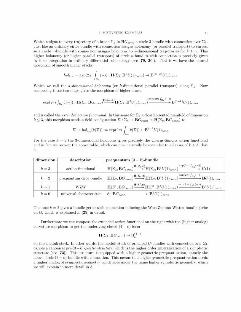
1. MOTIVATING EXAMPLES 51
Which assigns to every trajectory of a brane Σk in BGconn a circle 3-bundle with connection over Σk.Just like an ordinary circle bundle with connection assigns holonomy (or parallel transport) to curves,so a circle n-bundle with connection assigns holonomy to k-dimensional trajectories for k ≤ n. Thishigher holonomy (or higher parallel transport) of circle n-bundles with connection is precisely givenby fiber integration in ordinary differential cohomology (see [79, 30]). That is we have the naturalmorphism of smooth higher stacks
holΣk := exp(2πi
∫Σk
(−)) : H(Σk,BnU(1)conn)→ B(n−k)U(1)conn
Which we call the k-dimensional holonomy (or k-dimensional parallel transport) along Σk. Nowcomposing these two maps gives the morphism of higher stacks
exp(2πi∫
Σkc(−)) : H(Σk,BGconn)
H(Σk,c)// H(Σk,B3U(1)conn)
exp(2πi∫Σk
(−))// B(3−k)U(1)conn
and is called the extended action functional. In this sense for Σk a closed oriented manifold of dimensionk ≤ 3, this morphism sends a field configuration ∇ : Σk → BGconn in H(Σk,BGconn) to
∇ 7→ holΣk(c(∇)) := exp(2πi
∫Σk
c(∇)) ∈ B3−kU(1)conn
For the case k = 3 the 3-dimensional holonomy gives precisely the Cherns-Simons action functionaland in fact we recover the above table, which can now naturally be extended to all cases of k ≤ 3, thatis
dimension description prequantum (3− k)-bundle
k = 3 action functional H(Σ3,BGconn)H(Σ3,c)// H(Σ3,B
3U(1)conn)exp(2πi
∫Σ3
(−))// U(1)
k = 2 prequantum circe bundle H(Σ2,BGconn)H(Σ2,c)// H(Σ2,B
3U(1)conn)exp(2πi
∫Σ2
(−))// BU(1)conn
k = 1 WZW H(S1,BGconn)H(S1,c)// H(S1,B3U(1)conn)
exp(2πi∫S1 (−))
// B2U(1)conn
k = 0 universal characteristic c : BGconn // B3U(1)conn
The case k = 2 gives a bundle gerbe with connection inducing the Wess-Zumino-Witten bundle gerbeon G, which is explained in [29] in detail.
Furthermore we can compose the extended action functional on the right with the (higher analog)curvature morphism to get the underlying closed (4− k)-form
H(Σk,BGconn)→ Ω(4−k)cl
on this moduli stack. In other words, the moduli stack of principal G-bundles with connection over Σkcarries a canonical pre-(3−k)-plectic structure, which is the higher order generalization of a symplecticstructure (see [73]). This structure is equipped with a higher geometric prequantization, namely theabove circle (3− k)-bundle with connection. This means that higher geometric prequantization needsa higher analog of symplectic geometry which goes under the name higher symplectic geometry, whichwe will explain in more detail in 3.
52 4. HIGHER GEOMETRIC PERSPECTIVE
1.2. σ-models. A σ-model is supposed to be a type of model for quantum field theory. The basicidea is that we have some kind of space X, which we call the target space, and a space Σ, called theworldvolume, mapping into this target space. These fields φ : Σ→ X form together the configurationspace of fields or the trajectories of the brane Σ in X, which is the mapping stack H(Σ, X). Theσ-model describes the propagation of the worldvolume on the target space by a gauge field on X underwhich the worldvolume is charged. This is called the background gauge field of the σ-model.
The example of 3d Chern-Simons theory is a particular example of a σ-model, where the targetspace is BGconn and the worldvolume is closed oriented manifold Σk for k ≤ 3. The configuration spaceof fields on Σk is the mapping stack H(Σk,BGconn) and can be seen as the trajectories of the braneΣk in BGconn. The propagation of the worldvolume on the target space is given by the backgroundgauge field of the 3d Chern Simons theory, which is here given by the extended Lagrangian via theholonomy map
c : BGconn → B3U(1)conn
For example we have the notion of higher parallel transport over a worldvolume Σ3, which is given bythe holonomy map
∇ 7→ holc(∇)(Σ3) := exp(2πi
∫Σ3
c(∇)) ∈ U(1)
Which sends the trajectory ∇ : Σ3 → BGconn to elements in U(1) and which corresponds precisely tothe (exponentiated) action functional of 3d Chern-Simons theory.
This example of 3d Chern-Simons theory as a σ-model is also a blueprint for a more generalconstruction. For this one takes for the target space the universal moduli stack of field configurationsitself which we denote by Fields. For every closed oriented worldvolume Σk we have the mappingstack H(Σk,Fields) which is the configuration space of fields on Σk and the background gauge field isgiven by the extended Lagrangian, that is the map
L : Fields→ BnU(1)conn
of the universal higher stack to the n-stack of prinicpal circle n-bundles with connections. The La-grangian L induces Lagrangian data in arbitrary codimension, that is for every closed oriented world-volume Σk of dimension k ≤ n there is a transgressed Lagrangian
H(Σk,Fields)H(Σk,L)// H(Σk,B
nU(1)conn)exp(2πi
∫Σk
(−))// B(n−k)U(1)conn
defining the prequantum circle (n−k)-bundle of the given field theory. The curvature of these bundlesinduce the canonical pre-(n−k)-plectic structure on the moduli stack of field configurations on Σk. Incodimension 0, that is for k = n one has the holonomy map which is given by the morphism of stacks
exp(2πi
∫Σn
(−)) : H(Σn,Fields)→ U(1)
which reduce to the (exponentiated) action functional by taking global sections over the point andpassing to equivalence classes
exp(2πi
∫Σn
(−)) : Field configurations/equiv→ U(1)
Furthermore by postcomposing with the curvature morphism we get
ω : FieldsL→ BnU(1)conn
F(−)→ Ωn+1cl
2. HIGHER PREQUANTUM GEOMETRY 53
which shows that the stack of field configurations is naturally equipped with a pre-n-plectic structure,hence these are examples of σ-models with (pre)-n-plectic targets.
We saw above that in 3d Chern-Simons theory as a σ-model, we had an action functional with astarget the stack BGconn. This target space is equipped with the pre-3-plectic form
〈F(−) ∧ F(−)〉 : BGconn → Ω4cl
This binary dependence of the invariant polynomial 〈−,−〉 is an important feature of a whole tower ofσ-models. This tower of σ-models goes under the name AKSZ σ-models (see [26]) and are determinedby binary non-degenerate invariant polynomials. These AKSZ σ-models form a large class of σ-modelsand include ordinary 3d Chern-Simons theory, the Poisson σ-model, the Courant σ-model and higherdimensional abelian Chern-Simons theory. The Poisson σ-model can be seen as the perturbative partof the 2d Chern-Simons theory, which we will see later in this chapter.
2. Higher prequantum geometry
In the first section we indicated how higher prequantum geometry has a natural formulation interms of stacks. This section will give you a brief outline of the basic construction and facts abouthigher geometry, which can be read in full detail in [79]. We will start by describing the fields assmooth higher stacks.
2.1. Fields as smooth higher stacks. A field theory associates to a spacetime Σ the config-uration space of fields on Σ. We saw already in the above case that this configuration space of fieldsis richer than just a plain set. It needs to carry some smooth structure, which allows us to considersmooth maps from certain test spaces into Fields. This smooth structure allows us to perform vari-antional calculus on the configuration space of fields in order to find the critical locus of the actionfunctional. But actually there is more structure and that is that the action functional should also beinvariant under gauge transformation of the field configurations. One would like to have a configurationspace of fields that also contains all the information of the gauge transformations. This is achieved byconsidering the configuration space of fields on Σ as a smooth (Lie) groupoid, that is a groupoid withsmooth structure, instead of a manifold. A field theory where the configurations spaces of fields carrysuch a notion of gauge transformations is called a gauge theory. It is precisely this extra structurewhich allows us to treat the symplectic groupoid as a configuration space of fields over the point,instead of just the Poisson manifold. The objects of a symplectic groupoid can be seen as the fieldconfigurations on the point and the morphisms between these objects are the gauge transformationsbetween the fields.
More generally, there may also be gauge transformations between gauge transformations, and soon, meaning that there are higher groupoids. In mathematical terms, these data define an∞-category,where the objects are the fields, the 1-morphisms are the gauge transformations, the 2-morphisms arethe gauge of gauge transfomrations, and so on, and since gauge transformations are always invertiblewe have that every k-morphism is invertible for k ≥ 1 and hence one has that the ∞-category of fieldsis an ∞-groupoid. These ∞-groupoids can be seen as the particular simplicial sets, known as Kancomplexes[24]. This gives us the following assignment
Fields : Smooth manifolds→∞-groupoids
The fields and their gauge transformations between them can be restricted to smaller regions of space-time and more generally, they can be pulled back along smooth maps between different spacetimes.This means that this assignment is contravariant, which makes Fields a simplicial presheaf on the siteof smooth manifolds taking values in Kan complexes.
These ∞-groupoids we described so far are all discrete and do not have any smooth structure. Inthe previous case we treated the smooth manifold M secretly as the (simplicial) presheaf Fields which

54 4. HIGHER GEOMETRIC PERSPECTIVE
assigns to a smooth manifold Σ the set of smooth maps from Σ into M . In this way a smooth manifoldM can be realized as a (simplicial) presheaf on the category of smooth manifolds. Now suppose thatΣ is a manifold with a open cover Ui, then by definition the smooth map Σ → M can be obtainedby gluing smooth maps Ui →M that agrees on the overlap. This makes the presheaf
M : SmoothMfdop → Set
U 7→ C∞(U,M)
into a sheaf on the category of smooth manifolds. Moreover, since every manifold can be obtained bygluing Cartesian spaces, i.e. those smooth manifolds diffeomorphic to Rn for some n, we see that allthe information about M is in fact already encoded in the restriction of the sheaf to the category ofCartesian spaces and smooth maps between them
M : CartSpop → Set
In the case where Fields is a groupoid or a higher groupoid , we want a similar gluing construction. Inthe groupoid case, we should really glue by specifying gauge transformations on overlapping regions,and in the case of 2-groupoids, we should glue by specifying also gauge transformation between gaugetransformations on triple overlaps, and so on. A presheaf of∞-groupoids satisfying such a gluing law iscalled a simplicial sheaf or a∞-stack. This gluing condition precisely means that a field theory can becompletely described in terms of local data, since Fields can be probed by local patches diffeomorphicto Cartesian spaces.
2.2. Smooth ∞-stacks. Actually the precise formulation of the intuitive notion of a∞-stack onthe site of Cartesian space requires a bit of work and can be found in [79, 28], we will briefly recallhere the important concepts to place us in the right setting. To begin, we recall that a sheaf on thesite of Cartesian spaces is a presheaf M : CartSpop → Set such that for each Cech nerve C(Ui)→ Uthe morphism A(U) ' [CartSpop,Set](U,A) 7→ [CartSpop,Set](C(Ui, A) is an isomorphism, whereC(Ui) is the colimit of C(Ui), this is called the descent condition or sheaf condition. The higheranalog of this should give us the simplicial sheaf or the ∞-stack.
This may be achieved by equipping the category of simplicial presheaves [CartSpop, sSet], that isthe category whose objects are simplicial presheaves over Cartesian spaces, and whose morphisms arenatural transformations between them, with a model category structure. The notion of a model categorystructure provide a way to study∞-categories. A model category structure is a category equipped withthree classes of morphisms, the weak equivalences, fibrations and cofibrations, which satisfy certainconditions (see [54]). The fundamental example is the presentation of ∞-groupoids in terms of Kancomplexes by the standard Quillen model structure sSetQuillen on the category of simplicial sets. Weare interested in the so called simplicial model categories, which are the sSetQuillen-enriched modelcategories. The simplicial localization of a simplicial model category gives us a ∞-category. Notethat not every ∞-category comes from a simplicial model category. Now the category of simplicialpresheaves [CartSpop, sSet] is naturally a sSet-enriched category and together with a model structureit becomes a (combinatorial) simplicial model category, which is called the global projective modelcategory structure [CartSpop, sSet]proj , that is
(i) the fibrations are those morphisms whose components over each object U ∈ CartSp is a Kanfibration of simplicial sets;
(ii) the weak equivalences are those morphisms whose component over each object is a weakequivalence in the Quillen model structure on simplicial sets;
(iii) the cofibrations are the morphisms having the right lifting property against the morphismsthat are both fibrations as well as weak equivalences.
This model structure presents the ∞-category of ∞-presheaves on the category of Cartesian spaces.We impose now an ∞-sheaf condition, in terms of another model structure on [CartSpop, sSet]. Write
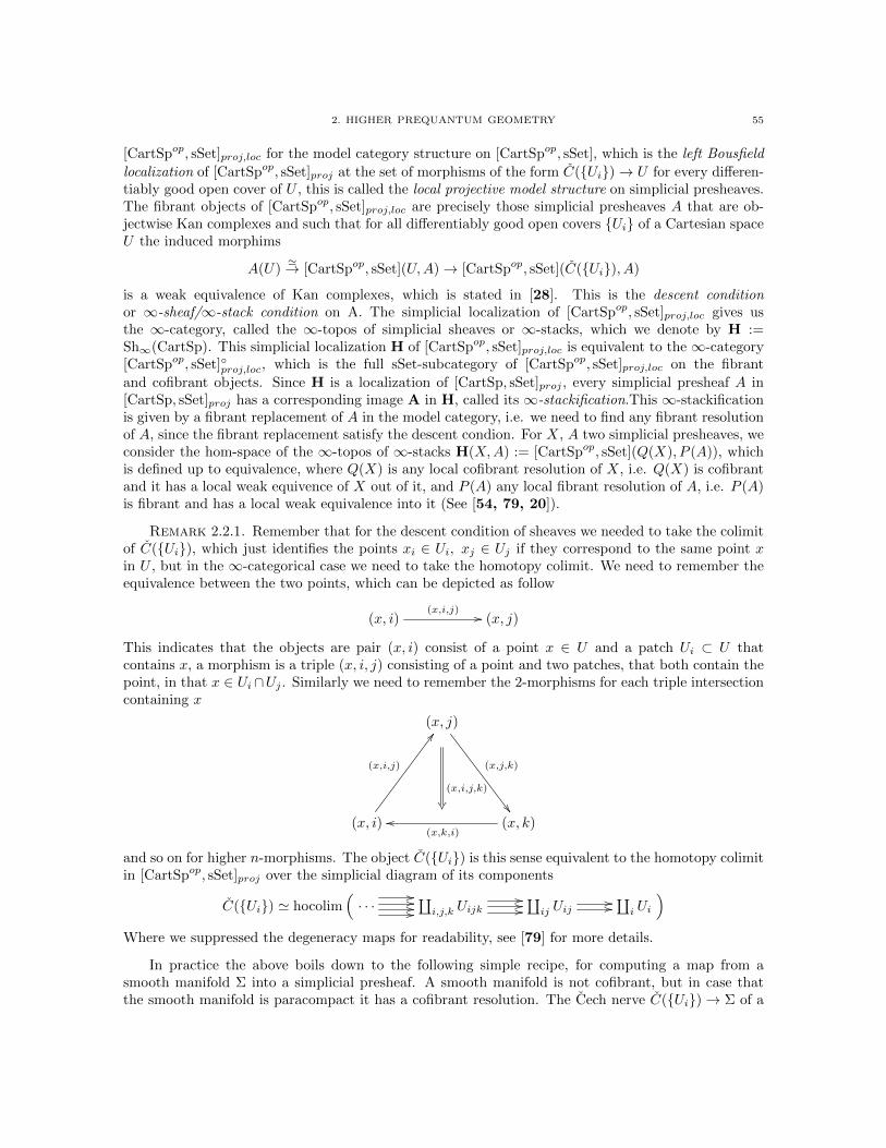
2. HIGHER PREQUANTUM GEOMETRY 55
[CartSpop, sSet]proj,loc for the model category structure on [CartSpop, sSet], which is the left Bousfield
localization of [CartSpop, sSet]proj at the set of morphisms of the form C(Ui)→ U for every differen-tiably good open cover of U , this is called the local projective model structure on simplicial presheaves.The fibrant objects of [CartSpop, sSet]proj,loc are precisely those simplicial presheaves A that are ob-jectwise Kan complexes and such that for all differentiably good open covers Ui of a Cartesian spaceU the induced morphims
A(U)'→ [CartSpop, sSet](U,A)→ [CartSpop, sSet](C(Ui), A)
is a weak equivalence of Kan complexes, which is stated in [28]. This is the descent conditionor ∞-sheaf/∞-stack condition on A. The simplicial localization of [CartSpop, sSet]proj,loc gives usthe ∞-category, called the ∞-topos of simplicial sheaves or ∞-stacks, which we denote by H :=Sh∞(CartSp). This simplicial localization H of [CartSpop, sSet]proj,loc is equivalent to the ∞-category[CartSpop, sSet]proj,loc, which is the full sSet-subcategory of [CartSpop, sSet]proj,loc on the fibrant
and cofibrant objects. Since H is a localization of [CartSp, sSet]proj , every simplicial presheaf A in[CartSp, sSet]proj has a corresponding image A in H, called its ∞-stackification.This ∞-stackificationis given by a fibrant replacement of A in the model category, i.e. we need to find any fibrant resolutionof A, since the fibrant replacement satisfy the descent condion. For X, A two simplicial presheaves, weconsider the hom-space of the ∞-topos of ∞-stacks H(X,A) := [CartSpop, sSet](Q(X), P (A)), whichis defined up to equivalence, where Q(X) is any local cofibrant resolution of X, i.e. Q(X) is cofibrantand it has a local weak equivence of X out of it, and P (A) any local fibrant resolution of A, i.e. P (A)is fibrant and has a local weak equivalence into it (See [54, 79, 20]).
Remark 2.2.1. Remember that for the descent condition of sheaves we needed to take the colimitof C(Ui), which just identifies the points xi ∈ Ui, xj ∈ Uj if they correspond to the same point xin U , but in the ∞-categorical case we need to take the homotopy colimit. We need to remember theequivalence between the two points, which can be depicted as follow
(x, i)(x,i,j) // (x, j)
This indicates that the objects are pair (x, i) consist of a point x ∈ U and a patch Ui ⊂ U thatcontains x, a morphism is a triple (x, i, j) consisting of a point and two patches, that both contain thepoint, in that x ∈ Ui∩Uj . Similarly we need to remember the 2-morphisms for each triple intersectioncontaining x
(x, j)
(x,j,k)
(x, i)
(x,i,j)
CC
(x, k)(x,k,i)
oo
(x,i,j,k)
and so on for higher n-morphisms. The object C(Ui) is this sense equivalent to the homotopy colimitin [CartSpop, sSet]proj over the simplicial diagram of its components
C(Ui) ' hocolim(· · ·
////////∐i,j,k Uijk
//////∐ij Uij
////∐i Ui
)Where we suppressed the degeneracy maps for readability, see [79] for more details.
In practice the above boils down to the following simple recipe, for computing a map from asmooth manifold Σ into a simplicial presheaf. A smooth manifold is not cofibrant, but in case thatthe smooth manifold is paracompact it has a cofibrant resolution. The Cech nerve C(Ui)→ Σ of a

56 4. HIGHER GEOMETRIC PERSPECTIVE
differentiably good open cover over a paracompact smooth manifold Σ is a cofibrant resolution of Σ in[CartSpop, sSet]proj,loc and so we write
C(Ui)∼loc // Σ
This follows from a cofibrancy criterion by Dugger[20]. From now on, we assume that the smoothmanifold Σ is paracompact and has a cofibrant resolution, which leaves us with the task of finding aversion Fields of a simplicial presheaf that is fibrant over CartSp. For describing the morphisms ofsimplicial sheaves from the smooth manifold Σ to Fields, we need to choose a differentiably good opencover Ui of Σ, form the Cech nerve simplicial presheaf C(Ui) and then consider spans of ordinarymorphisms of simplicial presheaves of the form
C(Ui)
∼loc
g // Fields
Σ
This diagram of simplicial presheaves presents an object in H(Σ,Fields) ' Fields(Σ), the hom-spaceof the ∞-topos of ∞-stacks. We call g : C(Ui) → Fields also a Fields-cocycle on Σ and on localdata it is given by a diagram
...
...
∐i,j,k Uijk
g(2)
//
Fields2
∐i,j Uij
g(1)
//
Fields1
∐i Ui
g(0)
// Fields0
of simplicial sets, where Fieldsk denote the set of k-simplices of Fields. This diagram gives a collection(gi, gij, gijk, · · · ), where
• gi is a 0-simplex in Fields(Ui)0 for any i;• gij is an 1-simplex in Fields(Uij)1 for any i, j, whose boundary 0-simplices are the restrictions
of gi and gj to Uij
gi|Uijgij // gj |Uij
• gijk is an 2-simplex in Fields(Uijk)2 for any i, j, k, whose boundary 1-simplices are therestrictions of gij ,gjk and gkl to Uijk
gj |Uijk
gjk|Uijk
gi|Uijk
gij |Uijk
BB
gk|Uijkgkl|Uijkoo
gijk

2. HIGHER PREQUANTUM GEOMETRY 57
• gijkl is a 3-simplex in Fields(Uijkl)3 for any i, j, k, l, which is of the form
gj |Uijklgjk|Uijkl // gk|Uijkl
gkl|Uijkl
gj |Uijklgjl|Uijkl
""
gjk|Uijkl // gk|Uijkl
gkl|Uijkl
gi|Uijkl
gik|Uijkl
<<
gij |Uijkl
OO
gil|Uijkl// gl|Uijkl gi|Uijkl
gij |Uijkl
OO
gil|Uijkl// gl|Uijkl
gijkl //
gijk|Uijkl
!)gikl|Uijkl
(
gjkl|Uijkl~
gijl|Uijkl~
• and so on
This description only gives the objects (i.e. the 0-morphism) of the ∞-groupoid Fields(Σ).The description of 1-morphisms in Fields(Σ) is straightforward. Let g and g′ be two objects of
Fields(Σ), then a 1-morphism h between them is the data of
• hi is a 1-simplex in Fields(Ui)1 for any i, whose boundary 0-simplices are gi and g′i, respec-tively
gihi // g′i
• hij is a ”square”, which can be thought of as pairs of 2-simplices in Fields(Uij)2 with acommon edge, whose boundary 1-simplices are as in the following diagram
gi|Uijgij
hi // g′i|Uijg′ij
gj |Uij hj
// g′j |Uij
hij
• and so on.
Similarly, one describes k-morphisms for any k ≥ 1.
2.3. Smooth higher stacks presented by Lie groupoids. A large class of examples of ∞-stacks are given by a presheaf of Kan complexes which sends a Cartesian space to the nerve of someLie groupoid.
Example 2.3.1. Let M be a smooth manifold. As said before M induces a sheaf, and in particulara presheaf, on CartSp, mapping a Cartesian space U to the set of smooth functions from U to M . Thissheaf can be seen as a stack or even more a ∞-stack in the above sense. To see this we may regardthis smooth manifold M as a Lie groupoid M with precisely one identity morphism for every objectin M , that is
M :=(M ×t sM
////// M//// M
)which can be depicted by
xId // x
for all x ∈ M . Now consider another smooth manifold Σ with differentiably good open cover Uithen we can associate canonically the Cech-groupoid C(Ui) to it, that is
C(Ui) =( ∐
i,j,k Uijk//////∐ij Uij
////∐i Ui
)

58 4. HIGHER GEOMETRIC PERSPECTIVE
which can be depicted by
(x, j)
(x,j,k)
(x, i)
(x,i,j)
CC
(x,i,k)// (x, k)
This Cech-groupoid inherits a smooth structure from the fact that Ui are smooth manifolds and theinclusions Ui → Σ are smooth functions, hence C(Ui) is a Lie groupoid. Then we have the canonicalprojection functor
C(Ui)→ Σ
(x, i) 7→ x
The notion of good open cover is needed in order to make this smooth functor a weak equivalence ofLie groupoids, in the sense that C(Ui) is cofibrant in a suitable model category structure on thecategory of Lie groupoids, this will be discussed later in more detail. To see that the Lie groupoid Mpresents a smooth stack follows from the fact that M give rise to a presheaf of groupoids on CartSpgiven by
U 7→ C∞(U,M)
To see that this serves as a presentation of the stack associated to this presheaf of groupoids, weconsider the functor C(Ui)→M which gives following diagram∐
i,j,k Uijkg(2)
//
M ×t sM
∐i,j Uij
g(1)
//
M
∐i Ui
g(0)
// M
Specifically this diagram gives a collection (gi, gij) where we have local maps gi : Ui → M forall i such that gij : Uij → M for every i, j is subject to the condition gi|Uij = sgij = tgij = gj |Uij(remember s = Id = t). This can be visualized by the simplicial diagram
gi|Uij= // gj |Uij
The condition for the 2-simplices are completely determined by this condition and hence the smoothmanifold M can be seen as a smooth stack M. This presentation of this Lie groupoid as a smoothstack can naturally be seen as a ∞-stacks, by taking the nerve over the presheaf of groupoids, sinceevery groupoid is mapped by the nerve functor N : Grpd → KanCplx to a Kan complex (see [54]).This gives us the presheaf of Kan complexes
U 7→ N(C∞(U,M))
that sends each Cartesian space U to the∞-groupoid N(C∞(U,M)). To describe the∞-stackification,which is also denoted by M, of this simplicial presheaf we need to say what the∞-groupoid associatedto a smooth manifold Σ is. By the above recipe we need take the Cech nerve as cofibrant resolution ofΣ, but this Cech nerve is precisely the nerve of the Cech-groupoid, hence applying the nerve functor
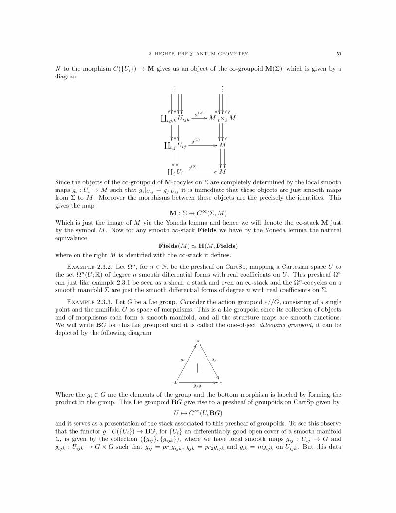
2. HIGHER PREQUANTUM GEOMETRY 59
N to the morphism C(Ui) → M gives us an object of the ∞-groupoid M(Σ), which is given by adiagram
...
...
∐i,j,k Uijk
g(2)
//
M ×t sM
∐i,j Uij
g(1)
//
M
∐i Ui
g(0)
// M
Since the objects of the∞-groupoid of M-cocyles on Σ are completely determined by the local smoothmaps gi : Ui → M such that gi|Uij = gj |Uij it is immediate that these objects are just smooth mapsfrom Σ to M . Moreover the morphisms between these objects are the precisely the identities. Thisgives the map
M : Σ 7→ C∞(Σ,M)
Which is just the image of M via the Yoneda lemma and hence we will denote the ∞-stack M justby the symbol M . Now for any smooth ∞-stack Fields we have by the Yoneda lemma the naturalequivalence
Fields(M) ' H(M,Fields)
where on the right M is identified with the ∞-stack it defines.
Example 2.3.2. Let Ωn, for n ∈ N, be the presheaf on CartSp, mapping a Cartesian space U tothe set Ωn(U ;R) of degree n smooth differential forms with real coefficients on U . This presheaf Ωn
can just like example 2.3.1 be seen as a sheaf, a stack and even an ∞-stack and the Ωn-cocycles on asmooth manifold Σ are just the smooth differential forms of degree n with real coefficients on Σ.
Example 2.3.3. Let G be a Lie group. Consider the action groupoid ∗//G, consisting of a singlepoint and the manifold G as space of morphisms. This is a Lie groupoid since its collection of objectsand of morphisms each form a smooth manifold, and all the structure maps are smooth functions.We will write BG for this Lie groupoid and it is called the one-object delooping groupoid, it can bedepicted by the following diagram
∗
gj
∗
gi
FF
gjgi// ∗
Where the gi ∈ G are the elements of the group and the bottom morphism is labeled by forming theproduct in the group. This Lie groupoid BG give rise to a presheaf of groupoids on CartSp given by
U 7→ C∞(U,BG)
and it serves as a presentation of the stack associated to this presheaf of groupoids. To see this observethat the functor g : C(Ui)→ BG, for Ui an differentiably good open cover of a smooth manifoldΣ, is given by the collection (gij, gijk), where we have local smooth maps gij : Uij → G andgijk : Uijk → G × G such that gij = pr1gijk, gjk = pr2gijk and gik = mgijk on Uijk. But this data
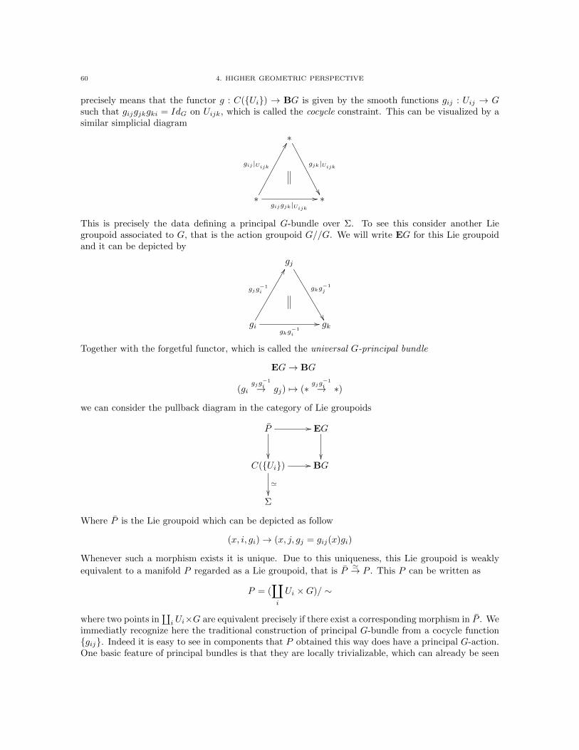
60 4. HIGHER GEOMETRIC PERSPECTIVE
precisely means that the functor g : C(Ui) → BG is given by the smooth functions gij : Uij → Gsuch that gijgjkgki = IdG on Uijk, which is called the cocycle constraint. This can be visualized by asimilar simplicial diagram
∗
gjk|Uijk
∗
gij |Uijk
FF
gijgjk|Uijk// ∗
This is precisely the data defining a principal G-bundle over Σ. To see this consider another Liegroupoid associated to G, that is the action groupoid G//G. We will write EG for this Lie groupoidand it can be depicted by
gj
gkg−1j
gi
gjg−1i
FF
gkg−1i
// gk
Together with the forgetful functor, which is called the universal G-principal bundle
EG→ BG
(gigjg−1i→ gj) 7→ (∗
gjg−1i→ ∗)
we can consider the pullback diagram in the category of Lie groupoids
P
// EG
C(Ui)
'
// BG
Σ
Where P is the Lie groupoid which can be depicted as follow
(x, i, gi)→ (x, j, gj = gij(x)gi)
Whenever such a morphism exists it is unique. Due to this uniqueness, this Lie groupoid is weakly
equivalent to a manifold P regarded as a Lie groupoid, that is P'→ P . This P can be written as
P = (∐i
Ui ×G)/ ∼
where two points in∐i Ui×G are equivalent precisely if there exist a corresponding morphism in P . We
immediatly recognize here the traditional construction of principal G-bundle from a cocycle functiongij. Indeed it is easy to see in components that P obtained this way does have a principal G-action.One basic feature of principal bundles is that they are locally trivializable, which can already be seen
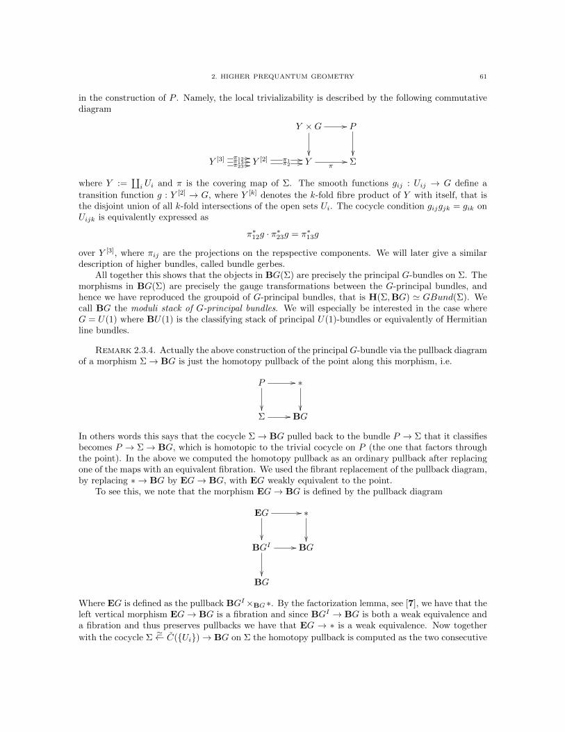
2. HIGHER PREQUANTUM GEOMETRY 61
in the construction of P . Namely, the local trivializability is described by the following commutativediagram
Y ×G
// P
Y [3] π12 //π13 //π23 // Y
[2] π1 //π2 // Y
π// Σ
where Y :=∐i Ui and π is the covering map of Σ. The smooth functions gij : Uij → G define a
transition function g : Y [2] → G, where Y [k] denotes the k-fold fibre product of Y with itself, that isthe disjoint union of all k-fold intersections of the open sets Ui. The cocycle condition gijgjk = gik onUijk is equivalently expressed as
π∗12g · π∗23g = π∗13g
over Y [3], where πij are the projections on the repspective components. We will later give a similardescription of higher bundles, called bundle gerbes.
All together this shows that the objects in BG(Σ) are precisely the principal G-bundles on Σ. Themorphisms in BG(Σ) are precisely the gauge transformations between the G-principal bundles, andhence we have reproduced the groupoid of G-principal bundles, that is H(Σ,BG) ' GBund(Σ). Wecall BG the moduli stack of G-principal bundles. We will especially be interested in the case whereG = U(1) where BU(1) is the classifying stack of principal U(1)-bundles or equivalently of Hermitianline bundles.
Remark 2.3.4. Actually the above construction of the principalG-bundle via the pullback diagramof a morphism Σ→ BG is just the homotopy pullback of the point along this morphism, i.e.
P
// ∗
Σ // BG
In others words this says that the cocycle Σ→ BG pulled back to the bundle P → Σ that it classifiesbecomes P → Σ→ BG, which is homotopic to the trivial cocycle on P (the one that factors throughthe point). In the above we computed the homotopy pullback as an ordinary pullback after replacingone of the maps with an equivalent fibration. We used the fibrant replacement of the pullback diagram,by replacing ∗ → BG by EG→ BG, with EG weakly equivalent to the point.
To see this, we note that the morphism EG→ BG is defined by the pullback diagram
EG
// ∗
BGI
// BG
BG
Where EG is defined as the pullback BGI×BG∗. By the factorization lemma, see [7], we have that theleft vertical morphism EG→ BG is a fibration and since BGI → BG is both a weak equivalence anda fibration and thus preserves pullbacks we have that EG → ∗ is a weak equivalence. Now together
with the cocycle Σ'← C(Ui)→ BG on Σ the homotopy pullback is computed as the two consecutive
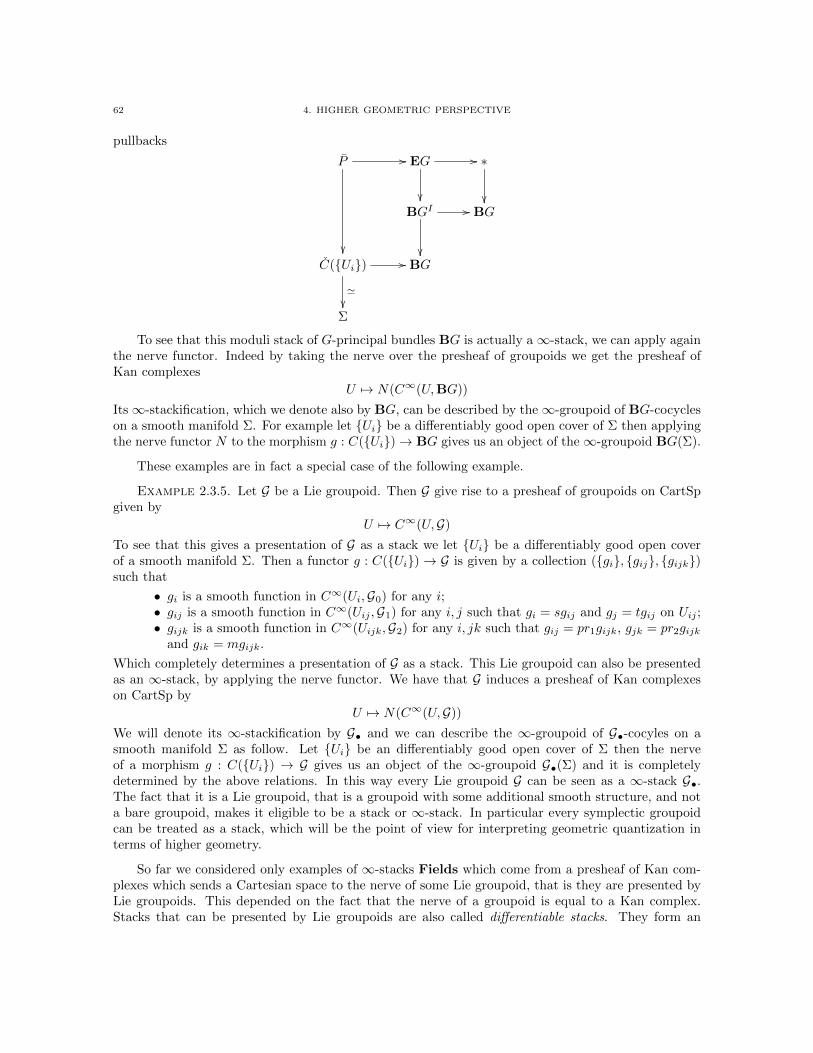
62 4. HIGHER GEOMETRIC PERSPECTIVE
pullbacks
P //
EG
// ∗
BGI
// BG
C(Ui)
'
// BG
Σ
To see that this moduli stack of G-principal bundles BG is actually a∞-stack, we can apply againthe nerve functor. Indeed by taking the nerve over the presheaf of groupoids we get the presheaf ofKan complexes
U 7→ N(C∞(U,BG))
Its∞-stackification, which we denote also by BG, can be described by the∞-groupoid of BG-cocycleson a smooth manifold Σ. For example let Ui be a differentiably good open cover of Σ then applyingthe nerve functor N to the morphism g : C(Ui)→ BG gives us an object of the∞-groupoid BG(Σ).
These examples are in fact a special case of the following example.
Example 2.3.5. Let G be a Lie groupoid. Then G give rise to a presheaf of groupoids on CartSpgiven by
U 7→ C∞(U,G)
To see that this gives a presentation of G as a stack we let Ui be a differentiably good open coverof a smooth manifold Σ. Then a functor g : C(Ui) → G is given by a collection (gi, gij, gijk)such that
• gi is a smooth function in C∞(Ui,G0) for any i;• gij is a smooth function in C∞(Uij ,G1) for any i, j such that gi = sgij and gj = tgij on Uij ;• gijk is a smooth function in C∞(Uijk,G2) for any i, jk such that gij = pr1gijk, gjk = pr2gijk
and gik = mgijk.
Which completely determines a presentation of G as a stack. This Lie groupoid can also be presentedas an ∞-stack, by applying the nerve functor. We have that G induces a presheaf of Kan complexeson CartSp by
U 7→ N(C∞(U,G))
We will denote its ∞-stackification by G• and we can describe the ∞-groupoid of G•-cocyles on asmooth manifold Σ as follow. Let Ui be an differentiably good open cover of Σ then the nerveof a morphism g : C(Ui) → G gives us an object of the ∞-groupoid G•(Σ) and it is completelydetermined by the above relations. In this way every Lie groupoid G can be seen as a ∞-stack G•.The fact that it is a Lie groupoid, that is a groupoid with some additional smooth structure, and nota bare groupoid, makes it eligible to be a stack or ∞-stack. In particular every symplectic groupoidcan be treated as a stack, which will be the point of view for interpreting geometric quantization interms of higher geometry.
So far we considered only examples of ∞-stacks Fields which come from a presheaf of Kan com-plexes which sends a Cartesian space to the nerve of some Lie groupoid, that is they are presented byLie groupoids. This depended on the fact that the nerve of a groupoid is equal to a Kan complex.Stacks that can be presented by Lie groupoids are also called differentiable stacks. They form an
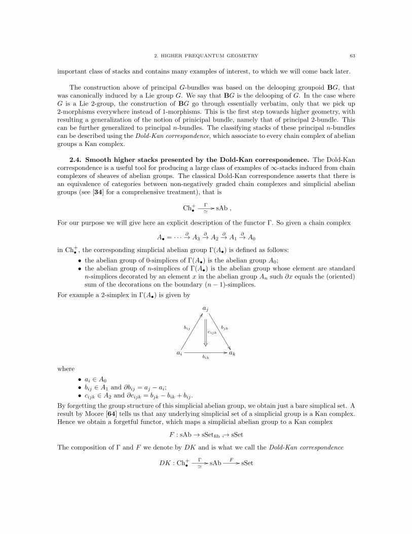
2. HIGHER PREQUANTUM GEOMETRY 63
important class of stacks and contains many examples of interest, to which we will come back later.
The construction above of principal G-bundles was based on the delooping groupoid BG, thatwas canonically induced by a Lie group G. We say that BG is the delooping of G. In the case whereG is a Lie 2-group, the construction of BG go through essentially verbatim, only that we pick up2-morphisms everywhere instead of 1-morphisms. This is the first step towards higher geometry, withresulting a generalization of the notion of prinicipal bundle, namely that of principal 2-bundle. Thiscan be further generalized to principal n-bundles. The classifying stacks of these principal n-bundlescan be described using the Dold-Kan correspondence, which associate to every chain complex of abeliangroups a Kan complex.
2.4. Smooth higher stacks presented by the Dold-Kan correspondence. The Dold-Kancorrespondence is a useful tool for producing a large class of examples of ∞-stacks induced from chaincomplexes of sheaves of abelian groups. The classical Dold-Kan correspondence asserts that there isan equivalence of categories between non-negatively graded chain complexes and simplicial abeliangroups (see [34] for a comprehensive treatment), that is
Ch+•
Γ
'// sAb ,
For our purpose we will give here an explicit description of the functor Γ. So given a chain complex
A• = · · · ∂→ A3∂→ A2
∂→ A1∂→ A0
in Ch+• , the corresponding simplicial abelian group Γ(A•) is defined as follows:
• the abelian group of 0-simplices of Γ(A•) is the abelian group A0;• the abelian group of n-simplices of Γ(A•) is the abelian group whose element are standardn-simplices decorated by an element x in the abelian group An such ∂x equals the (oriented)sum of the decorations on the boundary (n− 1)-simplices.
For example a 2-simplex in Γ(A•) is given by
aj
bjk
ai
bij
FF
bik
// ak
cijk
where
• ai ∈ A0
• bij ∈ A1 and ∂bij = aj − ai;• cijk ∈ A2 and ∂cijk = bjk − bik + bij .
By forgetting the group structure of this simplicial abelian group, we obtain just a bare simplical set. Aresult by Moore [64] tells us that any underlying simplicial set of a simplicial group is a Kan complex.Hence we obtain a forgetful functor, which maps a simplicial abelian group to a Kan complex
F : sAb→ sSetfib → sSet
The composition of Γ and F we denote by DK and is what we call the Dold-Kan correspondence
DK : Ch+•
Γ
'// sAb
F // sSet
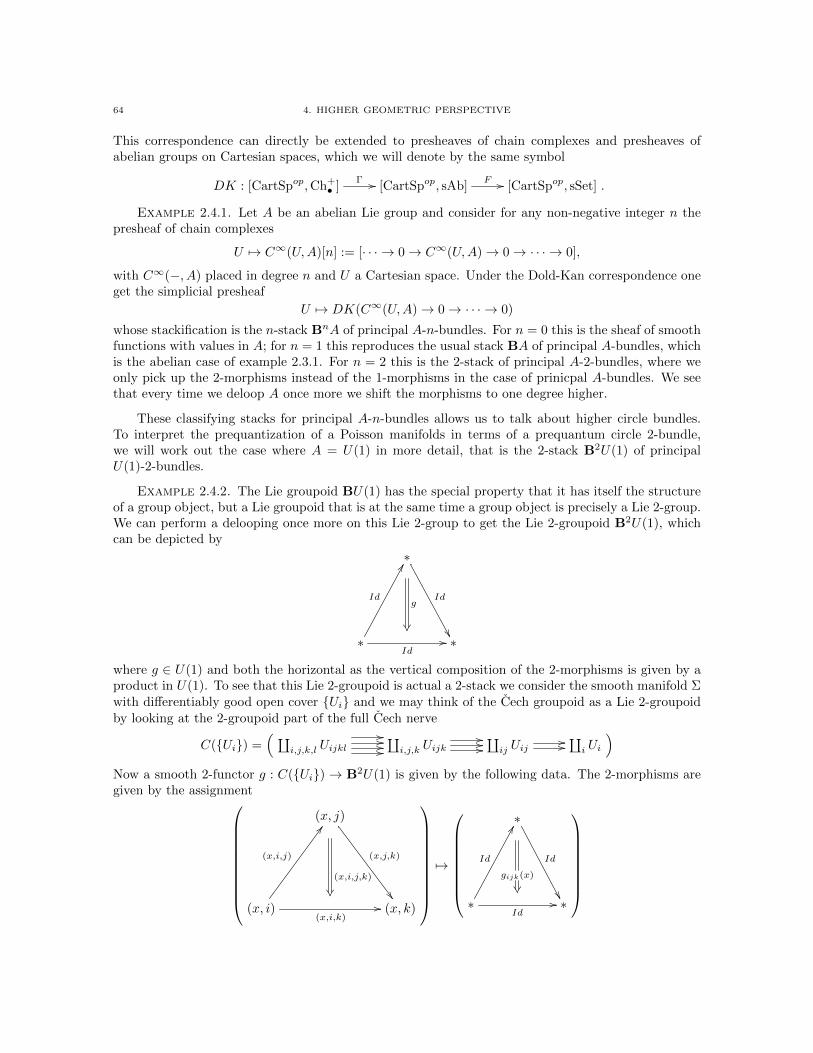
64 4. HIGHER GEOMETRIC PERSPECTIVE
This correspondence can directly be extended to presheaves of chain complexes and presheaves ofabelian groups on Cartesian spaces, which we will denote by the same symbol
DK : [CartSpop,Ch+• ]
Γ // [CartSpop, sAb]F // [CartSpop, sSet] .
Example 2.4.1. Let A be an abelian Lie group and consider for any non-negative integer n thepresheaf of chain complexes
U 7→ C∞(U,A)[n] := [· · · → 0→ C∞(U,A)→ 0→ · · · → 0],
with C∞(−, A) placed in degree n and U a Cartesian space. Under the Dold-Kan correspondence oneget the simplicial presheaf
U 7→ DK(C∞(U,A)→ 0→ · · · → 0)
whose stackification is the n-stack BnA of principal A-n-bundles. For n = 0 this is the sheaf of smoothfunctions with values in A; for n = 1 this reproduces the usual stack BA of principal A-bundles, whichis the abelian case of example 2.3.1. For n = 2 this is the 2-stack of principal A-2-bundles, where weonly pick up the 2-morphisms instead of the 1-morphisms in the case of prinicpal A-bundles. We seethat every time we deloop A once more we shift the morphisms to one degree higher.
These classifying stacks for principal A-n-bundles allows us to talk about higher circle bundles.To interpret the prequantization of a Poisson manifolds in terms of a prequantum circle 2-bundle,we will work out the case where A = U(1) in more detail, that is the 2-stack B2U(1) of principalU(1)-2-bundles.
Example 2.4.2. The Lie groupoid BU(1) has the special property that it has itself the structureof a group object, but a Lie groupoid that is at the same time a group object is precisely a Lie 2-group.We can perform a delooping once more on this Lie 2-group to get the Lie 2-groupoid B2U(1), whichcan be depicted by
∗
Id
∗
Id
FF
Id// ∗
g
where g ∈ U(1) and both the horizontal as the vertical composition of the 2-morphisms is given by aproduct in U(1). To see that this Lie 2-groupoid is actual a 2-stack we consider the smooth manifold Σwith differentiably good open cover Ui and we may think of the Cech groupoid as a Lie 2-groupoidby looking at the 2-groupoid part of the full Cech nerve
C(Ui) =( ∐
i,j,k,l Uijkl////////∐i,j,k Uijk
//////∐ij Uij
////∐i Ui
)Now a smooth 2-functor g : C(Ui) → B2U(1) is given by the following data. The 2-morphisms aregiven by the assignment
(x, j)
(x,j,k)
(x, i)
(x,i,j)
CC
(x,i,k)// (x, k)
(x,i,j,k)
7→
∗
Id
∗
Id
FF
Id// ∗
gijk(x)

2. HIGHER PREQUANTUM GEOMETRY 65
which is nothing more than a collection of smooth functions gijk : Uijk → U(1) for all i, j, k. On thesefunction a constraint is given by the 3-morphisms, since the only 3-morphism is the identity element,which is depicted by
(x, j) // (x, k)
(x, i)
<<OO
// (x, l)
'
'
⇒
(x, j)
""
// (x, k)
(x, i)
OO
// (x, l)
~
~
7→
∗ // ∗
∗
??OO
// ∗
gijk(x)
#
gikl(x) "
=
∗
// ∗
∗
OO
// ∗
gjkl(x)
gijl(x)
This gives the relation
gijk · gikl = gijl · gjklwhich is called the degree 2-cocycle constraint. These cocycles classify principal circle 2-bundles andto find such a principal circle 2-bundle, we need to construct the 2-functor EBU(1)→ B2U(1), whichis called the universal principal circle 2-bundle. Analogous to the case of example 2.3.3, we have thatEBU(1) can be depicted by
∗
cjk
∗
cij
FF
cik=cijcjkg// ∗
g
where cij , cjk, cik, g ∈ U(1) and all possible composition operations are given by the group product ofU(1). The universal principal circle 2-bundle is just the forgetful functor EBU(1) → B2U(1), whichforgets the labels ci of the 1-morphisms and just remembers the label g of the 2-morphism. Nowconsider the pullback diagram in the category of Lie 2-groupoids
P
// EBU(1)
C(Ui)
'
// B2U(1)
Σ
Where P is the Lie 2-groupoid whose objects are that of C(Ui), whose morphisms are morphismsin C(Ui) each equipped with a label c ∈ U(1), and whose 2-morphisms can be depicted as follow
(x, j)
cjk
(x, i)
cij
CC
cik// (x, k)
gijk(x)
which is subject to the condition
cjk = gijk(x)cijcjk

66 4. HIGHER GEOMETRIC PERSPECTIVE
Remark 2.4.3. More generally for arbitrary n ∈ N, this constuction models the homotopy pullbackof the point along a morphism Σ→ BnU(1), i.e.
P
// ∗
Σ // BnU(1)
Which together with the cofibrant replacement Σ'← C(Ui) → BnU(1) can be presented by the
ordinary pullback diagram
P
// EBn−1U(1)
' // ∗
C(Ui)
'
// BnU(1)
Σ
Where EBn−1U(1) is given by the image under DK of the complex of sheaves of abelian groups
U 7→ [· · · → 0→ C∞(U,U(1))Id→ C∞(U,U(1))→ 0→ · · · → 0]
and we have the obvious morphism EBn−1U(1) → BnU(1). To see that EBn−1U(1)'→ ∗ is a weak
equivalence, we note that the Dold-Kan correspondence takes quasi-isomorphisms to weak equivalencesin [CartSpop, sSet]proj , see[28], where a chain map is a quasi-isomorphism if it induces isomorphismson all homology groups. Since the above chain-complex has only trivial homology groups it is quasi-
isomorphic to the trivial chain-complex. Hence we have that EBn−1U(1)'→ ∗ (remember ∗ is given by
the image of DK of the complex of sheaves of trivial groups). For the case n = 2, this gives preciselythe above construction.
We saw before in example 2.3.3, that the pullback Lie 1-groupoid P was equivalent to the theprincipal 1-bundle P , as a Lie 0-groupoid, since whenever a morphism existed it was unique. Here wehave a similar situation, where every 2-morphism is unique if it exist, and hence here the Lie 2-groupoidP is equivalent to the Lie 1-groupoid
P =(C(Ui)2 × U(1)
// //// C(Ui)1 × U(1) //// C(Ui)0
)where the multiplication is given by
(x, i)cij→ (x, j)
cjk→ (x, k) = (x, i)cik=gijk(x)cijcjk→ (x, k)
But this precisely defines a groupoid central extension
BU(1)→ P → C(Ui) ' Σ
which are known in the literature as bundle gerbes over Σ with surjective submersion Y =∐i Ui → Σ.
A bundle gerbe is defined analogous to what remains of the locally trivialized principal U(1)-bundlein example 2.3.3, only we move up one step since we have delooped once more. Instead of a transitionfunction on Y [2] we take a principal U(1)-bundle P → Y [2] and since we cannot multiply U(1)-bundleslike the pullback of the transition function, the cocycle condition has to be relaxed to an isomorphismπ∗12P ⊗ π∗23P → π∗13P of U(1)-bundles over Y [3], which capture the groupoid multiplication on P ,which we demand to be associative. Explicitly, the above groupoid central extension is equivalently

2. HIGHER PREQUANTUM GEOMETRY 67
a bundle gerbe over a smooth manifold Σ together with a surjective submersion π : Y → Σ, which isdefined by a (principal) U(1)-bundle
P
p
Y [4]π123 //π124 //π134 //π234 // Y
[3] π12 //π13 //π23 // Y [2] π1 //
π2 // Y
π
Σ
over the the fiber product Y [2] := Y ×Σ Y = C(Ui)1 of morphisms, together with a bundle gerbemultiplication which is an isomorphism
σg : π∗12P ⊗ π∗23P → π∗13P
of U(1)-bundles on Y [3] = C(Ui)2, such that it is associative, in the sense that on Y [4] = C(Ui)3
the diagram
π∗12P ⊗ π∗23P ⊗ π∗34P
Id⊗π∗234σg
π∗123σg⊗Id // π∗13P ⊗ π∗34P
π∗134σg
π∗12P ⊗ π∗24P π∗124σg
// π∗14P
commutes. This bundle gerbe multiplication can be rephrased as a section σg of the U(1)-bundle
∂∗P ∗ → Y [3] (remember that ∂∗P ∗ = π∗12P∗⊗π∗13P ⊗π∗23P
∗). Moreover ∂∗σg is a section of ∂∗2P ∗ →Y [4], but ∂∗2P ∗ = π∗123∂
∗P ∗ ⊗ π∗124∂∗P ⊗ π∗134∂
∗P ∗ ⊗ π∗234∂∗P is canonically trivial so we have that
∂∗σg = 1, which is precisely the condition of associativity, see [65] . This bundle gerbe multiplicationσg is equivalent to the multiplication on P and the associativity condition is precisely the 2-cocyclecondition on g. So we find that bundle gerbes are presentations that are the total spaces of principalcircle 2-bundles.
In this example we considered a bundle gerbe over a smooth manifold Σ by considering Σ 'C(Ui) → B2U(1) as a central extension of the Cech groupoid over Σ by BU(1). But we areinterested in the case where we have a bundle gerbe over a symplectic groupoid Σ, which can beconsidered as a central extension of the symplectic groupoid Σ by BU(1). Let Σ be a symplecticgroupoid, which as in example 2.3.5 can be presented as a 2-stack. A morphism χ : Σ → B2U(1) of2-stack can similarly be described by a central groupoid extension
BU(1)→ P → Σ
And since U(1)-bundles are equivalent to Hermitian line bundles we have that this is eqiuvalent to aHermitian line bundle
L
p
Σ2
pr1 //m //pr2// Σ1
t //s// Σ0
over the space Σ1 of morphisms, together with an isomorphism
σ : pr∗1L⊗ pr∗2L→ m∗L

68 4. HIGHER GEOMETRIC PERSPECTIVE
of line bundles on Σ2, that is σ ∈ Γ(Σ2, ∂∗L∗) of norm 1 at every point, such that it satisfies the
associativity condition, which precisely is the cocycle condition on σ, as is stated in the definition 2.1.7of a prequantization of symplectic groupoid, that is ∂∗σ = 1.
2.5. Prequantization in terms of smooth higher stacks. So far we have classified the prin-cipal circle n-bundles by the ∞-stack BnU(1). For higher geometric prequantization we are moreinterested in principal n-bundles with the additional structure of a connection, in order to describe thethe prequantization of a symplectic groupoid. We will begin with the case of ordinary prequantizationof symplectic manifolds, where we need a differential refinement of BU(1) in order to describe theprincipal circle-bundle with connection.
Example 2.5.1. Let G be a Lie group with Lie algebra g. Consider the presheaf of groupoidswhich sends a Cartesian space U to the action groupoid Ω1(U ; g)//C∞(U,G), i.e. the 1-groupoid withthe set Ωn(U ; g) of g-valued 1-forms on U as objects and the group of smooth functions C∞(U,G)acting on Ω1(U ; g) via the gauge transformation
g : A 7→ g−1Ag + g−1dg
as set of morphisms, where here g−1Ag denotes pointwise the adjoint action of G on g and g−1dg isthe pullback g∗(θ) of the Maurer-Cartan form θ ∈ Ω1(G, g). This serves as a presentation of a stack,which we denote by BGconn, since for a smooth manifold Σ with a differentiably good open cover Uiit can be described by a collection (Ai, gij) consisting of
• Ai is a 1-form in Ω1(Ui, g) for any i;• gij is a smooth function in C∞(Uij , G) for any i, j such that Aj = g−1
ij Aigij +g−1ij dgij on Uij ;
• we have the cocycle constraint gijgjkgki = IdG on Uijk for any i, j, k.
Which corresponds to the simplicial diagram
Aj |Uijk
gjk|Uijk
Ai|Uijk
gij |Uijk
AA
gijgjk|Uijk// Ak|Uijk
These are readily seen to be the data defining a g-connection on a principal G-bundle over Σ. We findthat BGconn is the moduli stack of G-principal bundles with connection and we have H(Σ,BGconn) 'GBundconn(Σ). Furthermore we have an evident morphism of presheaves of groupoids
Ω1(−; g)//C∞(−;G)→ ∗//C∞(−;G)
which induces a forgetful morphism of stacks BGconn → BG which just forgets the connection.As a particular case of interest we consider G = U(1). In this case the ∞-stack BU(1)conn classifiesprincipal U(1)-bundles with connection. The presheaf of groupoids defining BU(1)conn can then beidentified with the presheaf of groupoids Ω1//C∞(−;U(1)) where the gauge transformation are givenby
g : A 7→ A+1
2πid log g
As in example 2.3.3 this describes precisely the connection ∇ on a U(1)-bundle P → Σ. For a coveringmap π : Y :=
∐i Ui → Σ, this connection ∇ defines a 1-from A ∈ Ω1(Y ), which is related to the
transition function g : Y [2] → U(1) by
π∗2A− π∗1A =1
2πid log g
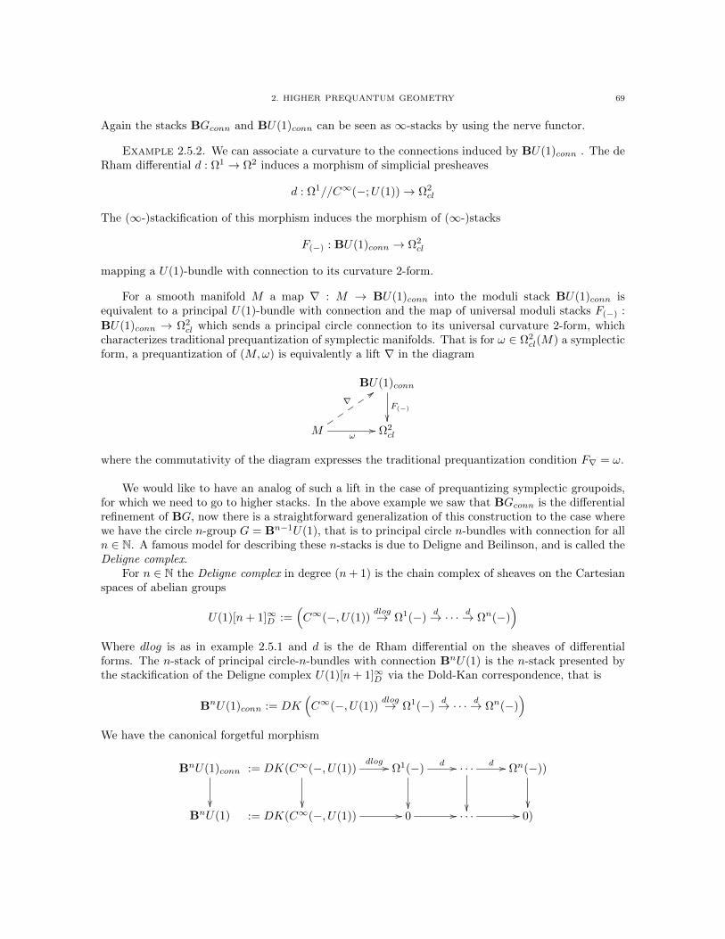
2. HIGHER PREQUANTUM GEOMETRY 69
Again the stacks BGconn and BU(1)conn can be seen as ∞-stacks by using the nerve functor.
Example 2.5.2. We can associate a curvature to the connections induced by BU(1)conn . The deRham differential d : Ω1 → Ω2 induces a morphism of simplicial presheaves
d : Ω1//C∞(−;U(1))→ Ω2cl
The (∞-)stackification of this morphism induces the morphism of (∞-)stacks
F(−) : BU(1)conn → Ω2cl
mapping a U(1)-bundle with connection to its curvature 2-form.
For a smooth manifold M a map ∇ : M → BU(1)conn into the moduli stack BU(1)conn isequivalent to a principal U(1)-bundle with connection and the map of universal moduli stacks F(−) :
BU(1)conn → Ω2cl which sends a principal circle connection to its universal curvature 2-form, which
characterizes traditional prequantization of symplectic manifolds. That is for ω ∈ Ω2cl(M) a symplectic
form, a prequantization of (M,ω) is equivalently a lift ∇ in the diagram
BU(1)conn
F(−)
M
∇::
ω// Ω2cl
where the commutativity of the diagram expresses the traditional prequantization condition F∇ = ω.
We would like to have an analog of such a lift in the case of prequantizing symplectic groupoids,for which we need to go to higher stacks. In the above example we saw that BGconn is the differentialrefinement of BG, now there is a straightforward generalization of this construction to the case wherewe have the circle n-group G = Bn−1U(1), that is to principal circle n-bundles with connection for alln ∈ N. A famous model for describing these n-stacks is due to Deligne and Beilinson, and is called theDeligne complex.
For n ∈ N the Deligne complex in degree (n+ 1) is the chain complex of sheaves on the Cartesianspaces of abelian groups
U(1)[n+ 1]∞D :=(C∞(−, U(1))
dlog→ Ω1(−)d→ · · · d→ Ωn(−)
)Where dlog is as in example 2.5.1 and d is the de Rham differential on the sheaves of differentialforms. The n-stack of principal circle-n-bundles with connection BnU(1) is the n-stack presented bythe stackification of the Deligne complex U(1)[n+ 1]∞D via the Dold-Kan correspondence, that is
BnU(1)conn := DK(C∞(−, U(1))
dlog→ Ω1(−)d→ · · · d→ Ωn(−)
)We have the canonical forgetful morphism
BnU(1)conn
BnU(1)
:= DK(C∞(−, U(1))
dlog // Ω1(−)
d // · · ·
d // Ωn(−))
:= DK(C∞(−, U(1)) // 0 // · · · // 0)
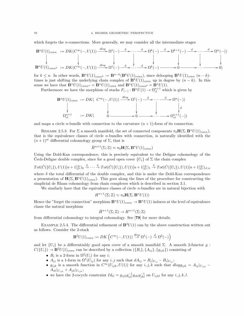
70 4. HIGHER GEOMETRIC PERSPECTIVE
which forgets the n-connections. More generally, we may consider all the intermediate stages
BnU(1)conn
BnU(1)connk
:= DK(C∞(−, U(1))
dlog // Ω1(−)
d // · · ·
d // Ωk(−)
d // Ωk+1(−)
d // · · ·
d // Ωn(−))
:= DK(C∞(−, U(1))
dlog // Ω1(−)d // · · · d // Ωk(−) // 0 // · · · // 0)
for k ≤ n. In other words, BnU(1)connk := Bn−k(BkU(1)conn), since delooping BkU(1)conn (n − k)-times is just shifting the underlying chain complex of BkU(1)conn up in degree by (n − k). In thissense we have that BnU(1)connn = BnU(1)conn and BnU(1)conn0 = BnU(1).
Furthermore we have the morphism of stacks F(−) : BnU(1)→ Ωn+1cl which is given by
BnU(1)conn
Ωn+1cl
:= DK(
:= DK(
C∞(−, U(1))
dlog // Ω1(−)
d // · · ·
d // Ωn(−))
d
0 // 0 // · · · // Ωn+1
cl (−))
and maps a circle n-bundle with connection to the curvature (n+ 1)-form of its connection.
Remark 2.5.3. For Σ a smooth manifold, the set of connected components π0H(Σ,BnU(1)conn),that is the equivalence classes of circle n-bundles with connection, is naturally identified with the(n+ 1)st differential cohomology group of Σ, that is
Hn+1(Σ;Z) ' π0H(Σ,BnU(1)conn)
Using the Dold-Kan correspondence, this is precisely equivalent to the Deligne cohomology of theCech-Deligne double complex, since for a good open cover Ui of Σ the chain complex
Tot(C(Ui), U(1)[n+ 1]∞D )0δ→ · · · δ→ Tot(C(Ui), U(1)[n+ 1]∞D )1
δ→ Tot(C(Ui), U(1)[n+ 1]∞D )cl,n
where δ the total differential of the double complex, and this is under the Dold-Kan correspondencea presentation of H(Σ,BnU(1)conn). This goes along the lines of the procedure for constructing thesimplicial de Rham cohomology from chain complexes which is described in section 3.1.
We similarly have that the equivalence classes of circle n-bundles are in natural bijection with
Hn+1(Σ;Z) ' π0H(Σ,BnU(1))
Hence the ”forget the connection” morphism BnU(1)conn → BnU(1) induces at the level of equivalenceclasse the natural morphism
Hn+1(Σ;Z)→ Hn+1(Σ;Z)
from differential cohomology to integral cohomology. See [79] for more details.
Example 2.5.4. The differential refinement of B2U(1) can by the above construction written outas follows. Consider the 2-stack
B2U(1)conn := DK(C∞(−, U(1))
dlog→ Ω1(−)d→ Ω2(−)
)and let Ui be a differentiably good open cover of a smooth manifold Σ. A smooth 2-functor g :C(Ui)→ B2U(1)conn can be described by a collection (Bi, Aij, gijk) consisting of
• Bi is a 2-form in Ω2(Ui) for any i;• Aij is a 1-form in Ω1(Uij) for any i, j such that dAij = Bj |Uij −Bi|Uij ;• gijk is a smooth function in C∞(Uijk, U(1)) for any i, j, k such that dloggijk = Aij |Uijk −Aik|Uijk +Ajk|Uijk ;
• we have the 2-cocycle constraint IdG = gijkg−1ijl giklg
−1jkl on Uijkl for any i, j, k, l.

2. HIGHER PREQUANTUM GEOMETRY 71
Which can be depicted by the simplicial diagram
Bj
Ajk
Bi
Aij
EE
Aik
// Bk
gijk
This data defines what is called a connective structure on the bundle gerbe from example 2.4.2. Itconsists of a connection on the U(1)-bundle P → Y [2] which defines a 1-form A ∈ Ω1(Y [2]) such thatthe isomorphism σg respects the connection, and of a 2-form B ∈ Ω2(Y ), called the curving, whichhas to be related to the connection on P by FA = π∗2B − π∗1B, where FA is the curvature of A.More precisely the connection A is called a bundle gerbe connection if it repsects the bundle gerbemultplication, that is if the section σg ∈ Γ(Y [3], ∂∗P ∗) satisfies σ∗g(∂∗A) = 0. If A is a bundle gerbe
connection, which always exists for bundle gerbes, then the curvature FA ∈ Ω2(Y [2]) satisfies ∂∗FA = 0and by exactness it follows that there must be a B ∈ Ω2(Y ) such that FA = ∂∗B = π∗2B − π∗1B. Thecollection (Bi, Aij, gijk) satisfying the above conditions gives precisely the local description ofthis. Consider a good open cover Ui of Σ with local sections si : Ui → Y and sections over the doubleoverlaps cij of (si, sj)
∗(P ) → Uij . Over triple overlaps we have that the bundle gerbe multiplicationdetermines the smooth functions gijk by σg(cij(x), cjk(x)) = gijk(x)cik(x). The 2-cocycle constraintcorresponds to the associativity condition on σg. The 1-form Aij is defined by Aij = (si, sj)
∗(A) andthe above condition on the Aij ’s is the fact that σg preserves the connection. The 2-form Bi is definedby Bi = s∗i (B) and the condition on the Bi’s is precisely the curvature condition. (See [65]).
Example 2.5.5. Consider the 2-stack
B2U(1)conn1 := DK(C∞(−, U(1))
dlog→ Ω1(−)→ 0)
By the forgetful morphims B2U(1)conn → B2U(1)conn1 we see that it gives the same data as theprevious example, only we need to forget everything about the 2-forms Bi, that is we just need toforget the curving. That is for a differentiably good open cover Ui of a smooth manifold Σ we havethat the smooth 2-functor g : C(Ui)→ B2U(1)conn1 can be described by a collection (Aij, gijk)consisting of
• Aij is a 1-form in Ω1(Uij) for any i, j• gijk is a smooth function in C∞(Uijk, U(1)) for any i, j, k such that dloggijk = Aij |Uijk −Aik|Uijk +Ajk|Uijk ;
• we have the 2-cocycle constraint IdG = gijkg−1ijl giklg
−1jkl on Uijkl for any i, j, k, l.
In this last example we recognize all the data that is needed for defining the prequantization ofa symplectic groupoid as defined in definition 2.1.7. Consider the symplectic groupoid Σ as a 2-stackand the morphism ∇1 : Σ → B2U(1)conn1 := B(BU(1)conn) of 2-stacks, which can be described by aHermitian line bundle
L
p
Σ2
pr1 //m //pr2// Σ1
t //s// Σ0
over the space Σ1 of morphisms, together with an element σ ∈ Γ(Σ2, ∂∗L∗), such that it is a cocycle
on σ and has a norm 1 at every point. The bundle gerbe connection gives a Hermitian connection ∇on the line bundle L such that it satisfies σ∗(∂∗∇) = 0, which precisely means that the cocycle σ is
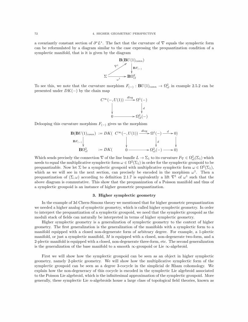
72 4. HIGHER GEOMETRIC PERSPECTIVE
a covariantly constant section of ∂∗L∗. The fact that the curvature of ∇ equals the symplectic formcan be reformulated by a diagram similar to the case expressing the prequantization condition of asymplectic manifold, that is it is given by the diagram
B(BU(1)conn)
BF(−)
Σ
∇199
ω1// BΩ2
cl
To see this, we note that the curvature morphism F(−) : BU(1)conn → Ω2cl in example 2.5.2 can be
presented under DK(−) by the chain map
C∞(−, U(1))
dlog // Ω1(−)
d
0 // Ω2
cl(−)
Delooping this curvature morphism F(−) gives us the morphism
B(BU(1)conn)
BF(−)
BΩ2
cl
:= DK(
:= DK(
C∞(−, U(1))
dlog // Ω1(−)
d
d // 0)
0 // Ω2
cl(−) // 0)
Which sends precisely the connection ∇ of the line bundle L→ Σ1 to its curvature F∇ ∈ Ω2cl(Σ1) which
needs to equal the multiplicative symplectic form ω ∈ Ω2(Σ1) in order for the symplectic groupoid to beprequantizable. Now let Σ be a symplectic groupoid with multiplicative symplectic form ω ∈ Ω2(Σ1),which as we will see in the next section, can precisely be encoded in the morphism ω1. Then aprequantization of (Σ, ω) according to definition 2.1.7 is equivalently a lift ∇1 of ω1 such that theabove diagram is commutative. This show that the prequanization of a Poisson manifold and thus ofa symplectic groupoid is an instance of higher geometric prequantization.
3. Higher symplectic geometry
In the example of 3d Chern-Simons theory we mentioned that for higher geometric prequantizationwe needed a higher analog of symplectic geometry, which is called higher symplectic geometry. In orderto interpret the prequantization of a symplectic groupoid, we need that the symplectic groupoid as themoduli stack of fields can naturally be interpreted in terms of higher symplectic geometry.
Higher symplectic geometry is a generalization of symplectic geometry to the context of highergeometry. The first generalization is the generalization of the manifolds with a symplectic form to amanifold equipped with a closed non-degenerate form of arbitrary degree. For example, a 1-plecticmanifold, or just a symplectic manifold, M is equipped with a closed, non-degenerate two-form, and a2-plectic manifold is equipped with a closed, non-degenerate three-form, etc. The second generalizationis the generalization of the base manifold to a smooth ∞-groupoid or Lie ∞-algebroid.
First we will show how the symplectic groupoid can be seen as an object in higher symplecticgeometry, namely 2-plectic geometry. We will show how the multiplicative symplectic form of thesymplectic groupoid can be seen as a degree 3-cocycle in the simplicial de Rham cohomology. Weexplain how the non-degeneracy of this cocycle is encoded in the symplectic Lie algebroid associatedto the Poisson Lie algebroid, which is the infinitesimal approximation of the symplectic groupoid. Moregenerally, these symplectic Lie n-algebroids house a large class of topological field theories, known as
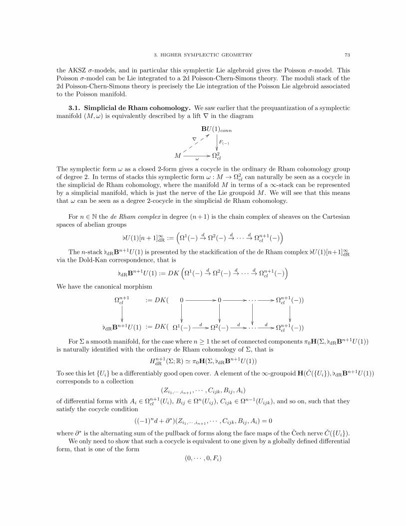
3. HIGHER SYMPLECTIC GEOMETRY 73
the AKSZ σ-models, and in particular this symplectic Lie algebroid gives the Poisson σ-model. ThisPoisson σ-model can be Lie integrated to a 2d Poisson-Chern-Simons theory. The moduli stack of the2d Poisson-Chern-Simons theory is precisely the Lie integration of the Poisson Lie algebroid associatedto the Poisson manifold.
3.1. Simplicial de Rham cohomology. We saw earlier that the prequantization of a symplecticmanifold (M,ω) is equivalently described by a lift ∇ in the diagram
BU(1)conn
F(−)
M
∇::
ω// Ω2cl
The symplectic form ω as a closed 2-form gives a cocycle in the ordinary de Rham cohomology groupof degree 2. In terms of stacks this symplectic form ω : M → Ω2
cl can naturally be seen as a cocycle inthe simplicial de Rham cohomology, where the manifold M in terms of a ∞-stack can be representedby a simplicial manifold, which is just the nerve of the Lie groupoid M . We will see that this meansthat ω can be seen as a degree 2-cocycle in the simplicial de Rham cohomology.
For n ∈ N the de Rham complex in degree (n+ 1) is the chain complex of sheaves on the Cartesianspaces of abelian groups
[U(1)[n+ 1]∞dR :=(
Ω1(−)d→ Ω2(−)
d→ · · · d→ Ωn+1cl (−)
)The n-stack [dRBn+1U(1) is presented by the stackification of the de Rham complex [U(1)[n+1]∞dR
via the Dold-Kan correspondence, that is
[dRBn+1U(1) := DK(
Ω1(−)d→ Ω2(−)
d→ · · · d→ Ωn+1cl (−)
)We have the canonical morphism
Ωn+1cl
[dRBn+1U(1)
:= DK(
:= DK(
0 //
0 //
· · · //
Ωn+1cl (−))
Ω1(−)
d // Ω2(−)d // · · · d // Ωn+1
cl (−))
For Σ a smooth manifold, for the case where n ≥ 1 the set of connected components π0H(Σ, [dRBn+1U(1))is naturally identified with the ordinary de Rham cohomology of Σ, that is
Hn+1dR (Σ;R) ' π0H(Σ, [dRBn+1U(1))
To see this let Ui be a differentiably good open cover. A element of the∞-groupoid H(C(Ui), [dRBn+1U(1))corresponds to a collection
(Zi1,··· ,in+1 , · · · , Cijk, Bij , Ai)of differential forms with Ai ∈ Ωn+1
cl (Ui), Bij ∈ Ωn(Uij), Cijk ∈ Ωn−1(Uijk), and so on, such that theysatisfy the cocycle condition
((−1)nd+ ∂∗)(Zi1,··· ,in+1, · · · , Cijk, Bij , Ai) = 0
where ∂∗ is the alternating sum of the pullback of forms along the face maps of the Cech nerve C(Ui).We only need to show that such a cocycle is equivalent to one given by a globally defined differential
form, that is one of the form
(0, · · · , 0, Fi)
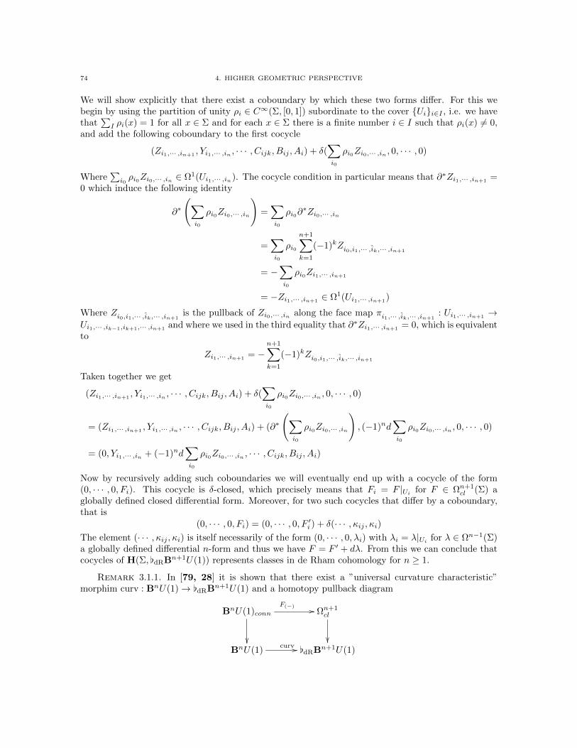
74 4. HIGHER GEOMETRIC PERSPECTIVE
We will show explicitly that there exist a coboundary by which these two forms differ. For this webegin by using the partition of unity ρi ∈ C∞(Σ, [0, 1]) subordinate to the cover Uii∈I , i.e. we havethat
∑I ρi(x) = 1 for all x ∈ Σ and for each x ∈ Σ there is a finite number i ∈ I such that ρi(x) 6= 0,
and add the following coboundary to the first cocycle
(Zi1,··· ,in+1 , Yi1,··· ,in , · · · , Cijk, Bij , Ai) + δ(∑i0
ρi0Zi0,··· ,in , 0, · · · , 0)
Where∑i0ρi0Zi0,··· ,in ∈ Ω1(Ui1,··· ,in). The cocycle condition in particular means that ∂∗Zi1,··· ,in+1 =
0 which induce the following identity
∂∗
(∑i0
ρi0Zi0,··· ,in
)=∑i0
ρi0∂∗Zi0,··· ,in
=∑i0
ρi0
n+1∑k=1
(−1)kZi0,i1,··· ,ik,··· ,in+1
= −∑i0
ρi0Zi1,··· ,in+1
= −Zi1,··· ,in+1 ∈ Ω1(Ui1,··· ,in+1)
Where Zi0,i1,··· ,ik,··· ,in+1is the pullback of Zi0,··· ,in along the face map πi1,··· ,ik,··· ,in+1
: Ui1,··· ,in+1 →Ui1,··· ,ik−1,ik+1,··· ,in+1
and where we used in the third equality that ∂∗Zi1,··· ,in+1= 0, which is equivalent
to
Zi1,··· ,in+1= −
n+1∑k=1
(−1)kZi0,i1,··· ,ik,··· ,in+1
Taken together we get
(Zi1,··· ,in+1 , Yi1,··· ,in , · · · , Cijk, Bij , Ai) + δ(∑i0
ρi0Zi0,··· ,in , 0, · · · , 0)
= (Zi1,··· ,in+1 , Yi1,··· ,in , · · · , Cijk, Bij , Ai) + (∂∗
(∑i0
ρi0Zi0,··· ,in
), (−1)nd
∑i0
ρi0Zi0,··· ,in , 0, · · · , 0)
= (0, Yi1,··· ,in + (−1)nd∑i0
ρi0Zi0,··· ,in , · · · , Cijk, Bij , Ai)
Now by recursively adding such coboundaries we will eventually end up with a cocycle of the form(0, · · · , 0, Fi). This cocycle is δ-closed, which precisely means that Fi = F |Ui for F ∈ Ωn+1
cl (Σ) aglobally defined closed differential form. Moreover, for two such cocycles that differ by a coboundary,that is
(0, · · · , 0, Fi) = (0, · · · , 0, F ′i ) + δ(· · · , κij , κi)The element (· · · , κij , κi) is itself necessarily of the form (0, · · · , 0, λi) with λi = λ|Ui for λ ∈ Ωn−1(Σ)a globally defined differential n-form and thus we have F = F ′ + dλ. From this we can conclude thatcocycles of H(Σ, [dRBn+1U(1)) represents classes in de Rham cohomology for n ≥ 1.
Remark 3.1.1. In [79, 28] it is shown that there exist a ”universal curvature characteristic”morphim curv : BnU(1)→ [dRBn+1U(1) and a homotopy pullback diagram
BnU(1)conn
F(−) // Ωn+1cl
BnU(1)
curv // [dRBn+1U(1)

3. HIGHER SYMPLECTIC GEOMETRY 75
of higher moduli stacks, which induces in cohomology the commutative diagram
Hn+1(Σ;Z)
F(−) // Ωn+1cl
Hn+1(Σ;Z)
curv // Hn+1dR (Σ;R)
Which shows that an integral cohomology class together with a closed differential form representingthe same class in de Rham cohomology can naturally be refined to a single object in differentialcohomology.
Analogous to the de Rham complex of differential forms of an ordinary manifold we have thesimplicial de Rham complex of a simplicial manifold. A simplicial manifold is a simplicial object in thecategory of smooth manifolds. We will here particularly be interested in simplicial manifolds that comefrom the nerve of a Lie groupoid G, which we will denote by G•. The de Rham complex of ordinarymanifolds can naturally be generalized to simplicial manifolds. Consider a simplicial manifold, say G•,then we have the double complex Ω•(G•), which is given by
· · · · · · · · ·
Ω1(G0)
d
OO
∂∗ // Ω1(G1)
d
OO
∂∗ // Ω1(G2)
d
OO
∂∗ // · · ·
Ω0(G0)
d
OO
∂∗ // Ω0(G1)
d
OO
∂∗ // Ω0(G2)
d
OO
∂∗ // · · ·
The boundary maps d : Ωk(Gn) → Ωk+1(Gn) are the usual derivatives of differential forms and ∂∗ :Ωk(Gn)→ Ωk(Gn+1), is the alternating sum of the pullback maps along the face maps of the simplicialmanifold. The total complex Tot(Ω•(G•)) of the double complex Ω•(G•) is the chain complex
Tot(Ω•(G•))0δ→ Tot(Ω•(G•))1
δ→ · · ·
whose components are the direct sums Tot(Ω•(G•))n =⊕
k+l=n Ωk(Gl) and whose total differential isgiven by δ = (−1)nd+ ∂∗, is called the simplicial de Rham complex. Under the Dold-Kan correspon-dence, this simplicial de Rham complex gives precisely a presentation of H(G•, [dRBnU(1))[79]. Thecohomology groups of this total complex are
HndR(G•;R) = Hn(Tot(Ω•(G•)))
and are called the simplicial de Rham cohomology groups of G. A cocycle [ω] ∈ HdR(G•;R) of degree nis a collection ω = (ω0
n, ω1n−1, · · · , ωn0 ) with ωkl ∈ Ωk(Gl) for k+ l = n, such that δω = 0. In particular
this means that dωn0 = 0 and ∂∗ω0n = 0, which means that similar to the argument above we can
add a coboundary such that we get a collection of the form ν = (0, ν1n−1, · · · , νn0 ) with νkl ∈ Ωk(Gl)
for k + l = n, which represents the same cocycle [ω] in the simplicial de Rham cohomology and wehave that ν is naturally an element in Ω1(Gn−1)⊕ · · · ⊕ Ωn−1(G1)⊕ Ωncl(G0). Here we recognize thata cocycle of the simplicial de Rham cohomology Hn
dR(G•;R) is precisely a cocycle in the ∞-groupoidH(G•, [dRBnU(1)), where we interpreted the simplicial manifold G• as a∞-stack. From which we canconclude that
HndR(G•;R) ' π0H(G•, [dRBnU(1))
In this sense for a symplectic manifold (M,ω), we can represent the symplectic form by themorphism of stacks ω : M → Ω2
cl → [dRB2U(1) and this morphism defines obviously a degree 2-cocycle in the simplicial de Rham cohomology.

76 4. HIGHER GEOMETRIC PERSPECTIVE
Similarly, the prequantization of a symplectic groupoid (Σ, ω) was equivalently a lift ∇1 of ω1 suchthat the following diagram commutes
B(BU(1)conn)
BF(−)
Σ
∇199
ω1// BΩ2
cl
This ω1 can be seen as a degree-3 cocycle in the simplicial de Rham cohomology. Since we haveobviously the map
ω1 : Σ→ BΩ2cl → [dRB3U(1)
which is equivalently an element
(0, ω, 0) ∈⊕
n=0,1,2
Ω3−n(Σn)
where ω ∈ Ω2(Σ1) is a symplective form, which is multiplicative, that is ∂∗ω = 0, but this preciselymeans that this element is a cocycle of degree 3 in the simplicial de Rham complex of Σ, instead ofa degree 2 cocycle for the case of a symplectic manifold. This observation shows that the symplecticgroupoid is really an object in higher symplectic geometry, namely 2-plectic geometry.
In order for these cocycles to be symplectic cocycles, we need to have a non-degeneracy condi-tion. The non-degeneracy condition of a symplectic form ω on a smooth manifold M means thatthe contraction map ι(−)ω : Γ(TM) → Ω1(M) is injective. Similarly a n-plectic form on a smooth
manifold M is a closed (n + 1)-form ω ∈ Ωn+1(M), which is non-degenerate, which means that thecontraction map ι(−)ω : Γ(TM) → Ωn(M) is injective (see [73]). This is the first generalization ofhigher symplectic geometry, where we generalize a 1-plectic manifold, that is a symplectic manifold,to a n-plectic manifold for arbitrary n ∈ N. The second generalization is the generalization of the basemanifold to a smooth ∞-stack or a Lie ∞-algebroid.
Remember that the infinitesimal approximation of a symplectic groupoid is the Poisson Lie al-gebroid associated to the Poisson manifold which integrates the symplectic groupoid. The cocyclefrom above has also an infinitesimal variant which is an invariant polynomial, which together form asymplectic Lie algebroid. Conversely, this invariant polynomial of the symplectic Lie algebroid can beintegrated to the above cocycle of the symplectic groupoid, see [79]. This is what we will treat in thenext sections.
3.2. Lie ∞-algebroids. A Lie algebroid serve the same role in the theory of Lie groupoidsthat Lie algebras serve in the theory of Lie groups. A Lie groupoid can be thought of as a Liegroup with many objects, similarly a Lie algebroid is like a Lie algebra with many objects. It is theinfinitesimal approximation to the Lie groupoid. We described a way to integrate a Lie algebroid to aparticular smooth groupoid, called a Lie groupoid. This integration can naturally extended to smooth∞-groupoids or smooth ∞-stacks, which we call the differential integration of an Lie ∞-algebroid toa smooth ∞-stack.
In these terms a n-plectic form on a Lie ∞-algebroid a can be described as an invariant poly-nomial ω on a which is (n + 1)-linear, that is ω ∈ Wn+1(a), and non-degenerate, which means thatι(−)ω : T a → Wn(a) is injective, where Wn(a) are the elements of the Weil algebra of a of degree n.In the case where a is a Lie 0-algebroid, a is just a smooth manifold X and W (a) = Ω•(X) the deRham algebra and an invariant polynomial is just a closed differential of positive degree n. Hence an-plectic form on a is just a closed (n+ 1)-form on X, such that ι(−)ω : Γ(TX)→ Ωn(X) is injective,which recovers our previous definition of a n-plectic form on a smooth manifold X.

3. HIGHER SYMPLECTIC GEOMETRY 77
A Lie ∞-algebroid is an infinitesimal approximation of a smooth ∞-groupoid.
Definition 3.2.1. The category of Lie∞-algebroids is the opposite category of the full subcategoryof cdgAlgopR
CE : L∞Algd → cdgAlgopRon graded-commutative cochain dg-algebras in non-negative degree whose underlying graded algebrais an exterior algebra over its degree-0 algebra, and this degree-0 algebra is the algebra of smoothfunctions on a smooth manifold.
Remark 3.2.2. This definition is in fact that of an affine C∞(X) Lie ∞-algebroid over a smoothmanifold X. But for this introductory discussion the above definition will suffice for the cases wetreat in this thesis and we don’t need to refine this to something more encompassing. For a fullcomprehensive account see [79].
In practice an object a ∈ L∞Algd may be identified (non-canonically) with a pair (CE(a), X),
(i) X is a smooth manifold, called the base space of the Lie ∞-algebroid;(ii) a is a non-positively graded C∞(X)-module degreewise of finite rank(iii) CE(a) = (∧•C∞(X) a
∗, dCE(a)) is a differential graded commutative algebra, called the Chevalley-
Eilenberg algebra of the Lie ∞-algebroid, where
∧•C∞(X) a∗ = C∞(X)⊕ a∗0⊕((a∗0 ∧C∞(X) a
∗0)⊕ a∗1)⊕ · · ·
with the kth summand on the right being in degree k and
dCE(a) : ∧•C∞(X) a∗ → ∧•C∞(X) a
∗
is a degree +1 derivation linear over the ground field such that d2CE(a) = 0.
If a is concentrated in degree 0 throught −(n− 1), then we speak of a Lie n-algebroid and if the basespace X = ∗ the point we speak of a Lie n-algebra.
Remark 3.2.3. An Lie ∞-algebroid with base space X = ∗ the point is an Lie ∞-algebra, orrather is the delooping of an Lie ∞-algebra. We write b g for Lie∞-algebroids over the point and theyform the full subcategory
b : L∞Alg → L∞Algd
of the traditional category of Lie ∞-algebras into that of Lie ∞-algebroids.
Example 3.2.4. For X = ∗ and a concentrated in degree 0 the finite dimensional Lie algebra g,we have that CE(a), where the underlying graded commutative algebra is the Grassmann algebra ong∗, that is
∧• g∗ = R⊕ g∗⊕(g∗ ∧ g∗)⊕ · · ·and where the Chevalley-Eilenberg differential dCE(g) of degree +1 is on g∗ the dual of the Lie bracket
dCE(g) := [−,−]∗ : g∗ → g∗ ∧ g∗
extended uniquely as a graded derivation on ∧• g∗. The fact that the Lie bracket satisfies the Jacobiidentity means precisely that the differential dCE(g) squares to 0, i.e. d2
CE(g) = 0. This CE(a) =
(∧• g∗, dCE(g)) is precisely the ordinary Chevalley-Eilenberg algebra. The Lie ∞-algebroid arising thisway can be written as a = b g, which is the delooping of g. This notation is the infinitesimal analog ofthe notation BG for the one-object delooping groupoid corresponding to the Lie group G.
Example 3.2.5. For X an arbitrary smooth manifold and a concentrated in degree 0, this isequivalent to the usual definition of a Lie algebroids as vector bundle E → X with anchor mapρ : E → TX, where we have CE(a) = (∧•C∞(X)Γ(E)∗, dCE(a)) and the anchor is encoded in the
map dCE(a) : C∞(X) → Γ(E)∗ which sends f 7→ ρ(−)(f) and can uniquely be extended to a gradedderivation on ∧•C∞(X)Γ(E)∗. For X = ∗ this definition indeed reproduces the previous example.
78 4. HIGHER GEOMETRIC PERSPECTIVE
Example 3.2.6. For n ∈ N the delooping of the line Lie n-algebra is the Lie ∞-algebroid bn−1Rdefined by the fact that CE(bn−1R) is generated over R from a single generator in degree n withvanishing differential.
Example 3.2.7. For X a smooth manifold and TX the tangent Lie algebroid, the correspondingChevalley-Eilenberg algebra is precisely the de Rham algebra of X, that is
CE(TX) = (Ω•(X), ddR)
Notice that Ω•(X) := ∧•C∞(X)Γ(T ∗X) and the anchor map ρ = Id.
Example 3.2.8. For (M,π) a Poisson manifold, where π ∈ ∧2Γ(TM) is the Poisson bivector, wehave the corresponding Poisson Lie algebroid B(M,π), see appendix A.0.1.13. The CE(B(M,π)),where the underlying graded commutative algebra is the Grassmann algebra on Γ(TM), that is∧•Γ(TM) the multivectors on M . Notice that the Poisson bivector π is an element of degree 2 in∧•Γ(TM). The Lie bracket on tangent vectors in Γ(TM) extends uniquely to a bracket [−,−]Sch onmultivector fields, called the Schouten bracket. It can be checked, see [75], that the Poisson bracket πsatisfies the Jacobi identity precisely if and only if π satisfies
[π, π]Sch = 0
This makes the Chevalley-Eilenberg differential
dCE(B := [π,−]Sch : ∧•Γ(TM)→ ∧•Γ(TM)
into a differential of degree +1 on multivector fields, that squares to 0. Hence the Poisson Lie algebroidis defined by
CE(B(M,π)) = (∧•Γ(TM), [π,−]Sch)
where π is the Poisson bivector.
For simplicity we assume for the moment that g is a Lie ∞-algebra. The generalization to Lie ∞-algebroids should be straightforward. ForX a smooth manifold, we can think ofHomdgAlg(CE(g),Ω•(X))as the set of Lie ∞-algebroid valued differential 1-forms, whose curvature form vanishes. We can seethis by first forgetting the differential structure and denoting
Ω•(X, g) := HomgrAlg(CE(g),Ω•(X)) ⊂ HomgrVect(CE(g),Ω•(X))
for the space of graded algebra homomorphisms from CE(g) to Ω•(X), which is a subspace of linearmaps (in particular of degree 0) from CE(g) to Ω•(X) as graded vector spaces. By definition CE(g)is freely generated generated algebra and is degreewise of finite rank and hence this is isomorphic tothe space of linear grading preserving maps HomgrVect(g
∗,Ω•(X)) from graded vector space g∗ of dualgenerators to Ω•(X) as a graded vector space. Since these maps are of degree 0 and recalling that gis non-positvely graded, this is is isomorphic to the space of elements of total degree 1 in elements ofΩ•(X) tensored with g
HomgrVect(g∗,Ω•(X)) ' (Ω•(X)⊗ g)1
The dg-algebra homomorphisms form a subspace of this space on those elements that respect thedifferential and is denoted by
Ω•(X, g)flat := HomdgAlg(CE(g),Ω•(X)) → HomgrAlg(CE(g),Ω•(X)) ' (Ω•(X)⊗ g)1
Under this equivalence these elements A in (Ω•(X) ⊗ g)1 satisfy a certain condition. By a simplecomputations, one finds that this condition is precisely the flatness constraint, namely we have theMauer-Cartan equation
dA+ ∂A+ [A ∧A] + [A ∧A ∧A] + · · · = 0
where the differential d and ∧ are the operations in Ω•(X) and where [., ., · · · ] are the n-ary bracketsin the Lie ∞-algebra g and ∂ is the differential in the chain complex g. For g an ordinary Lie algebra

3. HIGHER SYMPLECTIC GEOMETRY 79
we only have the binary bracket and A ∈ Ω1(X) ⊗ g satisfies the ordinary Maurer-Cartan equationdA+ [A ∧A] = 0.
In order to describe the non-flat g-valued differential 1-forms by homomorphism of differentialgraded algebras we need to pass from the Chevalley-Eilenberg algebra to the Weil algebra, which wewill construct now. Consider the Lie∞-algebroid a with base space X, then we can form the Grassmanalgebra over C∞(X) on the graded C∞(X)-module Γ(T ∗X)⊕a∗⊕ a∗[1], where a∗[1] is the shifted copyof a∗, that is
∧•(Γ(T ∗X)⊕ a∗⊕ a∗[1])
This is equipped with the differential d defined on generators as follows
(i) d|C∞(X) = ddR is the ordinary de Rham differential with values in Ω1(X) := Γ(T ∗X);(ii) d|a∗ : a∗ → a∗[1] is the degree-shift isomorphism;(iii) and d vanishes on all remaining generators.
which can be extended uniquely as a graded derivation. This defines the tangent Lie ∞-algebroid Taof a by CE(Ta) = (∧•(Γ(T ∗X)⊕ a∗⊕ a∗[1]),d).
Example 3.2.9. Let X be a smooth manifold, as a Lie 0-algebroid it can be seen as a Lie ∞-algebroid. The tangent Lie ∞-algebroid TX, that is
CE(TX) = (∧•(Γ(T ∗X), ddR)
corresponds precisely to the tangent Lie algebroid TX as defined in example 3.2.7.
Example 3.2.10. For g an ordinary finite dimensional Lie algebra. The tangent Lie ∞-algebroidTg is given by
CE(Tg) = (∧•(g∗⊕ g∗[1]),d)
where d : g∗ → g∗[1] is the grade shifting isomorphism on the generators, which can be extended asa graded derivation. The notion of the ordinary Weil algebra W (g), see [12], can be defined as theChevalley-Eilenberg algebra of this tangent Lie ∞-algebroid, it has
• as underlying graded algebra the graded algebra of the tangent Lie ∞-algebroid Tg, that is
∧•(g∗⊕ g∗[1])
• equipped with a differential on the copy g∗
dW (g)|g∗ = dCE(g) + d
where dCE(g) acts on g∗ as the differential of the Chevalley-Eilenberg algebra of g and isextended uniquely to the shifted generators g∗[1] by the graded commutativity
dCE(g)d = −ddCE(g)
which in turn can be extended as a graded derivation to ∧•(g∗⊕ g∗[1]).
This defines the ordinary Weil algebra
W (g) = CE(Tg) = (∧•(g∗⊕ g∗[1]), dW (g))
Remark 3.2.11. This abstract construction of the Weil algebra W (g) looks a bit arbitrary, butin fact it is the unique dg-algebra free on the underlying graded vector space such that the projectionmorphism i∗ : g∗⊕ g∗[1] → g∗ of graded vector spaces extends to a dg-homomophism i∗ : W (g) →CE(g) (see [28, 76, 77]).
This notion of the ordinary Weil algebra for Lie algebras can be extended to Lie ∞-algebras andLie ∞-algebroids. Analogous to the previous example we define the Weil algebra of a Lie ∞-algebroida as the Chevalley-Eilenberg algebra of the tangent Lie ∞-algebroid Ta.
80 4. HIGHER GEOMETRIC PERSPECTIVE
Definition 3.2.12. The Weil algebra of an Lie∞-algebroid a with base space X, is the differentialgraded commutative algebra
W (a) := (∧•(Γ(T ∗X)⊕ a∗⊕ a∗[1]), dW (a))
where the differential is the sum
dW (a) = dCE(a) + d
of two degree +1 graded derivations, where d acts on the generators as above and dCE(a) acts on theunshifted elements in a∗ as the differential of the Chevalley-Eilenberg algebra of a and is extendeduniquely to shifted generators by the graded commutativity
dCE(g)d = −ddCE(g)
Furthermore dCE(a) vanishes on C∞(X)
Remark 3.2.13. The correct definition of the Weil algebra of a Lie∞-algebroid, as stated in [26],should be over Lie∞-algebroids with in degree 0 an arbitrary R-algebra A. The Weil algebra is definedas a representative of the free smooth dg-algebra on the underlying graded A-modules such that theprojection morphism i∗ : Ω•(A)⊕a∗⊕ a∗[1]→ a∗ of graded A-modules extends to a dg-homomorphismi∗ : W (a) → CE(a) (see [28, 76, 77]). We will focus here on the special case where the R-algebrais the smooth algebra C∞(X) of smooth functions over a smooth manifold X, for which we gave theexplicit definition.
Example 3.2.14. Let g be a Lie algebra, then the definition of W (b g) recovers precisely theordinary definition of the Weil algebra as in example 3.2.10.
Example 3.2.15. Let a = X be an ordinary smooth manifold, then W (X) = Ω•(X), that is theordinary de Rham algebra of X.
Example 3.2.16. Let a = bn−1R be the delooping of the line Lie n-algebra, then W (bn−1R) isthe free dg-algebra on a single generator c in degree n. In other words it is the graded algebra of twogenerators c and γ, with c in degree n and γ in degree n + 1 together with a differential dW (bn−1R)
defined by sending c to γ.
For g a Lie ∞-algebra, W (g) is the unique dg-algebra free on the underlying graded vector spaceg∗ such that the canonical projection i∗ : W (a)→ CE(a) is a dg-homomorphism. Due to the freenessof W (g) we have an isomorphism
Ω•(X, g) = HomgrAlg(CE(g),Ω•(X)) ' HomdgAlg(W (g),Ω•(X))
from which we conclude that HomdgAlg(W (g),Ω•(X)) is the collection of total degree 1 differentialform with values in the Lie ∞-algebra g. Consider a morphism
(A,FA) : W (g)→ Ω•(X)
Then by similar computation as for finding the Maurer-Cartan equations one finds that
FA = dA+ ∂A+ [A ∧A] + [A ∧A ∧A] + · · ·
and precisely if the curvature vanish, that is FA = 0, then this morphism factors through the Chevalley-Eilenberg algebra
CE(g)
∃AflatzzΩ•(X) W (g)
Aoo
OO
in which case we call A flat.
3. HIGHER SYMPLECTIC GEOMETRY 81
3.3. Cocycles, invariant polynomials and Chern-Simons elements.
Definition 3.3.1. For a a Lie ∞-algebroid and n ∈ N, a cocycle in degree n on a is an elementµ ∈ CE(a) which is dCE(a)-closed, i.e. dCE(a)µ = 0.
Since bn−1R is the Lie ∞-algebroid whose Chevalley-Eilenberg algebra has a single generator indegree n and a trivial differential, a cocycle µ in degree n on a is presicely given by a morphism ofdg-algebras µ : CE(bn−1R)→ CE(a) or dually by a morphism of Lie ∞-algebroids µ : a→ bn−1R.
Example 3.3.2. Let a = b g be the delooping of a Lie algebra g, a cocycle on a of degree ncorresponds precisely with a traditional Lie algebra cocycle on g of degree n.
Example 3.3.3. Let X be a smooth manifold, a cocycle in degree n of the tangent Lie∞-algebroidTX is precisely a closed n-form on X.
Definition 3.3.4. An invariant polynomial on a is an dW (a)-closed element 〈−〉 in ∧•(Γ(T ∗X)⊕a∗[1]) ⊂W (a).
The property 〈−〉 ∈ ∧•(Γ(T ∗X) ⊕ a∗[1]) says that for any v ∈ a and ιv : W (a) → W (a) thecontraction derivation, we have
ιv〈−〉 = 0 (horizontality)
Together with the second property dW (a)〈−〉 = 0 this implies that for the Lie derivative
Lv := [dW (a), ιv]
in W (a) along v ∈ a, which encodes the coadjoint action of a on W (a), we have
Lv〈−〉 = 0 (ad-invariance)
Example 3.3.5. Let a = b g be the delooping of an ordinary Lie algebra g. The above encodesprecisely the classical definition of adg-invariant polynomials. Indeed, for a Lie algebra g, the conditiondW (a)〈−〉 = 0 implies precisely the adg-invariance of an element 〈−〉 ∈ ∧•(g∗[1]).
Example 3.3.6. Let a = X be a smooth manifold, seen as a Lie 0-algebroid, an invariant polyno-mial of degree n is a closed differential form of degree n.
Definition 3.3.7. Let 〈−〉 ∈ W (a) be an invariant polynomial on a Lie ∞-algebroid, we say acocycle µ ∈ CE(a) is in transgression with 〈−〉 if there exists an element cs ∈W (a) such that
(i) dW (a)cs = 〈−〉;(ii) i ∗ cs = µ
We say that cs is a Chern-Simons element witnessing this transgression.
The above ingredients can be summarized in the following diagram
CE(a) CE(bn−1R)µoo
W (a)
OO
W (bn−1R)
OO
(cs,〈−〉)oo
inv(a)
OO
inv(bn−1R)
OO
〈−〉oo
For the full construction of this commuting diagram we refer the reader to [28, 79].
Remember from the motivating example 1 of 3d Chern-Simons theory that we talked about trans-gressing an cocycle via a Chern-Simons element to an invariant polynomial. There the Chern-Simons
82 4. HIGHER GEOMETRIC PERSPECTIVE
element played the role of the Lagrangian of the theory, which maps a g-valued 1-form A to a differen-tial form CS(A). Actually the above transgression encodes precisely this information, remember thatthe dg-algebra morphisms Ω•(Σ)←W (g) : (A,FA) are in natural bijection with the degree 1 g-valueddifferential forms. Hence we write
Ω•(Σ)A←W (g)
cs←W (bn+1R) : cs(A)
for the differential form associated by the Chern-Simons element cs to the degree 1 g-valued differentialform A, and call this the Chern-Simons differential form associated to A. This differential formcs(A) ∈ Ω•(Σ) can be integrated to the corresponding (higher) Chern-Simons action functional
S〈−〉 : A 7→∫
Σ
cs(A)
Similarly, for 〈−〉 an invariant polynomial on g, we write
Ω•(Σ)clA←W (g)
〈−〉← inv(bn+1R) : 〈FA〉Which we call the curvature characteristic form of A with repspect to 〈−〉.
Since we can pick g any Lie ∞-algebroid, the above constitute not only 3d Chern-Simons theory,but a whole class of action functionals which go under name of∞-Chern-Simons theory. We will see inthe next section how this construction secretly encodes the generalization of the ordinary Chern-Weilhomomorphism to the full ∞-Chern-Weil homomorphism in ∞-Chern-Weil theory.
Remark 3.3.8. The degree 1 g-valued differential form on Σ should be thought of a (non-trivial)g-valued connection on a trivial principal ∞-bundle on Σ. Remember in our example of 3d Chern-Simons theory the principal G-bundle on a 3-dimensional smooth manifold Σ can always be trivialized.This principal G-bundle on Σ can be obtained via universal integration of g, which we will treat in thesection 3.5.
In the case of 3d Chern-Simons theory we transgressed a cocycle to a binary invariant polynomial.For our purpose it suffice to consider only a certain class of binary invariant polynomials, namely theclass of binary invariant polynomials that constitute what we call a symplectic Lie n-algebroid.
Definition 3.3.9. A symplectic Lie n-algebroid (B, ω) is a Lie n-algebroid B that is equippedwith a quadratic non-degenerate invariant polynomial ω ∈W (B) of degree n+ 2.
This definition means that for each chart U → X where X is the base manifold of B, there is abasis xi for CE(B |U ) such that
ω =1
2ωijdx
i ∧ dxj
with ωij ∈ R → C∞(X) and deg(xi) + deg(xj) = n. The non-degeneracy condition precisely meansthat the coefficient matrix ωij has an inverse and furthermore we have that dW (B)ω = 0. Thesesymplectic Lie n-algebroids (B, ω) are important for us, since these invariant polynomials ω are non-degenerate and hence they are (n + 1)-plectic forms on the Lie n-algebroid B. We will give now twoexamples that are important for us.
Example 3.3.10. (Symplectic manifold: n = 0) A Lie 0-algebroid is just a smooth manifold M . Aquadratic non-degenerate invariant polynomial of degree 2 on M is precisely a non-degenerate closed2-form ω ∈ Ω2(M), that is a symplectic 2-form. Hence a symplectic manifold being a pair (M,ω) is asymplectic Lie 0-algebroid.
Example 3.3.11. (Poisson manifold: n = 1) For a Poisson manifold (M,π), with Poisson bivectorπ ∈ ∧2Γ(TX), we have the corresponding Poisson Lie algebroid B(M,π). The Chevalley-Eilenbergalgebra of the Poisson Lie algebroid is given by
CE(B(M,π)) = (∧•Γ(TM), dCE(B) = [π,−]Sch)

3. HIGHER SYMPLECTIC GEOMETRY 83
which is explained in example 3.2.8. Now if we work locally, that is if we consider a chart U →M , thenthe underlying graded algebra of CE(B(M,π)|U ) is generated from degree 0 elements xi and degree1 elements ∂i, since the underlying graded algebra is free over C∞(U) (remember it is a Grassmannalgebra).The Poisson bivector can be written as
π = −1
2πij∂i ∧ ∂j
which is evidently a Lie algebroid cocycle since
dCE(B)π = [π, π]Sch = 0
Acting with the differential dCE(B) on the generators gives us
dCE(B)xi = [π, xi]Sch = −1
2[πjk∂j ∧ ∂k, xi]Sch
=1
2∂j ∧ ∂k ∧ [πjk, xi]− 1
2πjk∂k ∧ [∂j , x
i] +1
2πjk∂j ∧ [∂k, x
i]
= −πij∂jWhere we used that [∂j , x
i] = L∂j xi = dxi(∂j) is the Lie derivative of ∂j along the smooth function
xi. Similarly
dCE(B)∂i = [π, ∂i]Sch = −1
2[πjk∂j ∧ ∂k, ∂i]Sch
=1
2∂j ∧ ∂k ∧ [πjk, ∂i]−
1
2πjk∂k ∧ [∂j , ∂i] +
1
2πjk∂j ∧ [∂k, ∂i]
=1
2
∂πjk
∂xi∂j ∧ ∂k = 0
Where [∂j , ∂i] = 0. By definition, the Weil algebra W (B(M,π)) is generated from elements xi and ∂i,together with their shifted partners dxi and d∂i, and it has the differential
dW (B) = [π,−]Sch + d
Which acts on the generators xi and ∂i as
dW (B)xi = −πij∂j + dxi
dW (B)∂i = d∂i
Now consider element
cs = ∂i ∧ dxi + π ∈W (B)
We will show that this element cs is a Chern-Simons element transgressing the cocycle π to an invariantpolynomial, say ω. First we have obviously the property that
i∗cs = cs|∧•Γ(TM) = π
For the second property of a Chern-Simons element, lets rewrite cs in terms of dW (B) instead of d,this is
cs = ∂i ∧ dW (B)xi − π
Then
dW (B)cs = dW (B)∂i ∧ dW (B)xi − dW (B)π
= d∂i ∧ (−πij∂j) + d∂i ∧ dxi − dπ
= d∂i ∧ dxi
= dxi ∧ d∂i =: ω

84 4. HIGHER GEOMETRIC PERSPECTIVE
Where in the second equality we used that dW (B)π = dπ, since π is cocycle, in the third equality weused that
dπ = −1
2
∂πjk
∂xi∂j ∧ ∂k ∧ dxi − πjkd∂j ∧ ∂k
And in the last equality we used that W (B) has an underlying commutative algebra and since thedegree of d∂i and dxi is 2 and 1 respectively, they have to commute like this. Furthermore thisω is an non-degenerate invariant polynomial of degree 3, since it is a dW (B)-closed element ω ∈∧•(Γ(T ∗M) ⊕ Γ(TM)[1]) that is obviously non-degenerate. We conclude that for a Poisson manifold(M,π) with Poisson bivector π = πij∂i ∧ ∂j , the pair
(B(M,π), ω = dxi ∧ d∂i)
consisting of the Poisson Lie algebroid B(M,π) and of the invariant polynomial ω that is in transgres-sion with the cocycle π, is a symplectic Lie algebroid.
3.4. Poisson σ-model. We saw in the example of previous section that there are certain sym-plectic Lie algebroids where the invariant polynomial is in transgression with a cocycle, via a Chern-Simons element. More generally, if a symplectic Lie n-algebroid (B, ω) give rise to a triple (π, cs, ω),consisting of a Chern-Simons element transgressing an invarient polynomial ω to a cocycle π, then thisdefines an AKSZ σ-model action, see for the full proof of this result [26]. The AKSZ constuction is amathematical formulation to unify a large class of topological field theories, known as AKSZ σ-models[1].
This AKSZ σ-model has as target space the tangent Lie∞-algebroid TB. The configuration spaceof fields is the space of maps Maps(TΣ,TB) from the worldsheet Σ to TB. Dually, this is space ofdg-morphisms from W (B) to Ω•(Σ), i.e. the space of degree 1 B-valued differential forms on Σ. As wesaw before, a degree 1 B-valued differential form A on Σ maps the Chern-Simons element cs ∈W (B)to a differential form cs(A) on Σ. Integrating this differential form on Σ will give an AKSZ σ-modelaction
Maps(TΣ,TB)→ R
A 7→∫
Σ
cs(A)
Example 3.4.1. (Poisson σ-model) Let (M,π) be a Poisson manifold, with Poisson bivector π =πij∂i ∧ ∂j and let (B(M,π), ω = dxi ∧ d∂i) be the corresponding symplectic Lie algebroid. Then theinvariant polynomial ω is in transgression with the cocycle π via the Chern-Simons element
cs = ∂i ∧ dW (B)xi − π
Let Σ a 2-dimensional oriented compact manifold and consider the dg-morphism
Ω•(Σ)←W (B) : (X, η)
which is a Poisson Lie algebroid valued differential form on Σ.This is just given by a vector bundlemorphism TΣ → T ∗M from the tangent bundle TΣ to the cotangent bundle T ∗M . Such a map isin components a smooth function X : Σ → M and a 1-form η ∈ Ω1(Σ, X∗(T ∗M)) with values in thepullback of the tangent bundle of M along X. The AKSZ action is∫
Σ
cs(X, η) =
∫Σ
η ∧ ddRX +1
2πij(X)ηi ∧ ηj
where ηi = η(∂i) and we used that X(dW (B)xi) = ddRX
i, since (X, η) is a dg-algebra homomorphism.This gives us precisely the Lagrangian of the Poisson σ-model (see [46, 8, 26]). The Poisson σ-modelis a 2-dimensional topological field theory with target a Poisson manifold (M,π), or rather the PoissonLie algebroid B(M,π) corresponding to that.
3. HIGHER SYMPLECTIC GEOMETRY 85
Similar to the construction of the Poisson σ-model Lagrangian on a 2-dimensional manifold, theordinary Chern-Simons theory action functional on a 3-dimensional manifold can also be constructedthis way. Here one takes the symplectic Lie 2-algebroid (b g, 〈−,−〉) where g is a semisimple Lie algebraand 〈−,−〉 the Killing form invariant polynomial. This invariant polynomial is in transgression withthe cocycle µ = − 1
6 〈−, [−,−]〉, via a Chern-Simons element cs ∈ W (b g). Under a g-valued formΩ•(Σ3)←W (b g) : A this element cs maps to the ordinary degree 3 Chern-Simons form
cs(A) = 〈A ∧ dA〉+1
3〈A ∧ [A ∧A]〉
For the full construction we refer the reader to [26, 23]. This ordinary Chern-Simons theory actionfunctional is in fact a special case of the Courant σ-model Lagrangian where the Lie 2-algebroid has asbase manifold the point. Besides these Poisson σ-model and Courant σ-model Lagrangians this AKSZσ-model construction contains higher abelian Chern-Simons functionals and many more examples ofinterest.
As said before these AKSZ σ-model actions form a special case of a larger class of action functionalswhich goes under the name of ∞-Chern-Simons theory. The AKSZ σ-model actions arise only fromthose triples (π, cs, ω) that come from a symplectic Lie n-algebroid. For the more general case, thesetriples form the infinitesimal data of the construction of the ∞-Chern-Weil homomorphism, whichgeneralizes the ordinary Chern-Weil homomorphism for ordinary Chern-Simsons theory. In the nextsection we show, how this infinitesimal data can be integrated to a morphisms of higher stacks, in thesame way as ordinary Chern-Simons theory is enhanced to a morphism from the stacks of principalG-bundles with connection to the 3-stack of circle 3-bundles with connections. In this way we willsee that the Poisson σ-model is the infinitesimal (or perturbative) versions of the Lie integrated 2dChern-Simons theory.
3.5. Lie ∞-integration. Ordinary Lie integration assigns to a Lie algebra g a Lie group G thatis infinitesimally modelled by g. We explained in appendix A how this is generalized to Lie algebroidsand Lie groupoids. In this section we discuss briefly the construction of Lie ∞-integration, that sendsa Lie ∞-algebroid to a smooth ∞-groupoid of which it is a infinitesimal approximation. For a morecomprehensive account, see [79, 28].
Definition 3.5.1. For a a Lie algebroid, let exp(a) ∈ H(CartSpop, sSet) be the simplicial presheaf,which for U ∈ CartSp and k ∈ N is given by the assignment
exp(a) : (U, [k]) 7→ Ω•(U ×∆k)vert,siAvert← CE(a)
where ∆k is the standard realization of the k-simplex as a smooth manifold with boundary and cornersand where Ω•(U ×∆•)vert,si is the dg-algebra of vertical differential forms on U ×∆k → U , that havesitting instants toward the boundary faces of the simplex. See [28] for details.
This simplicial presheaf presents the universal Lie integration of the Lie algebroid a. This Lieintegration of a always exists and in fact it is a smooth ∞-groupoid as in 2.2.
Proposition 3.5.2. [26, 28] For a an Lie ∞-algebroid, the simplicial presheaf exp(a) is a smooth∞-groupoid (is objectwise a Kan complex).
Example 3.5.3. Let G be the simply-connected Lie group integrating the Lie algebra g and BGits delooping Lie groupoid as in example 2.3.3. The simplicial presheaf exp(g) that we get by universalintegrating g can be truncated to the presheaf of groupoids BG. We denote by τ1(−) the truncationoperation that quotients out 2-morphisms in a simplicial presheaf to obtain a preseheaf of groupoids.Then we have an isomorphism
BG = τ1 exp(g)
To see this remember that the dg-algebra morphisms Ω•(∆k)← CE(g) are in natural bijection with theg-valued 1-forms that are flat, that is they have a curvature form that vanish. Now the 1-morphisms in

86 4. HIGHER GEOMETRIC PERSPECTIVE
exp(g) are U -parametrized families of flat g-valued 1-forms Avert on the interval ∆1, and 2-morphismsare U -parametrized families of flat g-valued 1-forms on the disk ∆2, interpolating between these 1-morphisms. By identifying theses 1-forms with the pullback of the Mauer-Cartan form θ on G wecan equivalently think of a 1-morphism as a based smooth path in G, i.e. there is a smooth pathγ : ∆1 → G such that Avert = γ∗θ ∈ Ω1(∆1, g). In this way we can think of 2-morphisms as smoothhomotopies relative endpoints between these smooth paths. Since G is simply-connected this meansthat after dividing out 2-morphisms only the endpoints of these paths γ remain, which we identifywith the point in G.
Example 3.5.4. Let a be a Lie algebroid A over a smooth manifold M , then this constructionapplied to a reproduces the integration method by A-paths of Crainic and Fernanded (see [17]). Thesimplicial presheaf exp(a) that we get by univeral integrating a can be truncated to the presheaf ofgroupoids G(A). We denote by τ1(−) again the truncation operation that quotients out 2-morphismsin a simplicial presheaf to obtain a presheaf of groupoids. Then we want to show that
G(A) = τ1 exp(a)
A 1-morphism in exp(a) is just an U -parametrized family of dg-algebra morphisms between theChevalley-Eilenberg algebra CE(a) and Ω•(∆1). But since Ω•(∆1) = CE(T∆1), where T∆1 is thetangent Lie algebroid of ∆1, we have that a dg-algebra morphism Ω•(∆1) ← CE(a) is dually a Liealgebroid morphism T∆1 → a. Now such a morphism of Lie algebroids is precisely equivalent to whatCrainic and Fernandes defined as an A-path a : ∆1 → A in the Lie algebroid a, see [16, 17] andappendix A for more details.
Analogous to the above situation for 1-morphisms, a 2-morphism in exp(a) is an U -parametrizedfamily of dg-algebra morphisms Ω•(∆2) ← CE(a), which is precisely a variation of A-paths, that in-terpolates between these 1-morphisms. The 2-morphims are precisely homotopies relative endpointsbetween these 1-morphisms. By applying the trunction τ1(−) to exp(a) we divide out the 2-morphismsand thus we divide out the homotopies between A-paths, which is precisely equivalent to the construc-tion of the Weinstein groupoid G(A). Furthermore the Weinstein groupoid G(A) is a topologicalgroupoid and we need to impose the condition integrability on a in order for G(A) to be a s-simplyconnected Lie groupoid.
Remark 3.5.5. There are some technicalities involved concerning composition of A-paths. InCrainic and Fernandes approach in [17] we needed to introduce some cut-off function in order for thecomposition of A-paths to be smooth instead of piecewise smooth. By universal Lie integration ofthe Lie algebroid, this is accomplished by concerning differential forms on U × ∆1 that have sittinginstants, as is explained in [28].
Remark 3.5.6. Although exp(a) is a smooth∞-groupoid, it is in general not degreewise a smoothmanifold. In order for this to be true, we need impose some extra integrability condition on a, which ingeneral are not known. For the case that a is a Lie algebroid, the integrability condition to integrate itto a Lie groupoid are studied by Crainic and Fernandes in [17], and we call the Lie algebroid integrableif it integrates to a Lie groupoid.
Example 3.5.7. Let n ≥ 1 and consider the line Lie n-algebra bn−1R. Then fiber integration oversimplices induces an equivalence ∫
∆•: exp(bn−1R)
'→ BnR
Which is proven in [28].
For a a a Lie ∞-algebroid, a dg-algebra homomorphism CE(a) ← CE(bn−1R) : µ is precisely acocycle, i.e. an element µ ∈ CE(a) that is dCE(a)-closed. Such a cocycle µ induces a morphism ofsimplicial presheaves
exp(µ) : exp(a)→ exp(bn−1R)
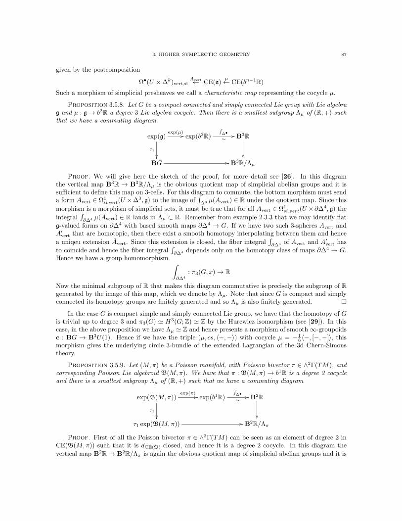
3. HIGHER SYMPLECTIC GEOMETRY 87
given by the postcomposition
Ω•(U ×∆k)vert,siAvert← CE(a)
µ← CE(bn−1R)
Such a morphism of simplicial presheaves we call a characteristic map representing the cocycle µ.
Proposition 3.5.8. Let G be a compact connected and simply connected Lie group with Lie algebrag and µ : g→ b2R a degree 3 Lie algebra cocycle. Then there is a smallest subgroup Λµ of (R,+) suchthat we have a commuting diagram
exp(g)
τ1
exp(µ) // exp(b2R)
∫∆•
∼// B3R
BG // B3R/Λµ
Proof. We will give here the sketch of the proof, for more detail see [26]. In this diagramthe vertical map B3R → B3R/Λµ is the obvious quotient map of simplicial abelian groups and it issufficient to define this map on 3-cells. For this diagram to commute, the bottom morphism must senda form Avert ∈ Ω1
si,vert(U ×∆3, g) to the image of∫
∆3 µ(Avert) ∈ R under the quotient map. Since this
morphism is a morphism of simplicial sets, it must be true that for all Avert ∈ Ω1si,vert(U ×∂∆4, g) the
integral∫∂∆4 µ(Avert) ∈ R lands in Λµ ⊂ R. Remember from example 2.3.3 that we may identify flat
g-valued forms on ∂∆4 with based smooth maps ∂∆4 → G. If we have two such 3-spheres Avert andA′vert that are homotopic, then there exist a smooth homotopy interpolating between them and hence
a uniqeu extension Avert. Since this extension is closed, the fiber integral∫∂∆4 of Avert and A′vert has
to coincide and hence the fiber integral∫∂∆4 depends only on the homotopy class of maps ∂∆4 → G.
Hence we have a group homomorphism ∫∂∆4
: π3(G, x)→ R
Now the minimal subgroup of R that makes this diagram commutative is precisely the subgroup of Rgenerated by the image of this map, which we denote by Λµ. Note that since G is compact and simplyconnected its homotopy groups are finitely generated and so Λµ is also finitely generated.
In the case G is compact simple and simply connected Lie group, we have that the homotopy of Gis trivial up to degree 3 and π3(G) ' H3(G;Z) ' Z by the Hurewicz isomorphism (see [29]). In thiscase, in the above proposition we have Λµ ' Z and hence presents a morphism of smooth∞-groupoidsc : BG → B3U(1). Hence if we have the triple (µ, cs, 〈−,−〉) with cocycle µ = − 1
6 〈−, [−,−]〉, thismorphism gives the underlying circle 3-bundle of the extended Lagrangian of the 3d Chern-Simonstheory.
Proposition 3.5.9. Let (M,π) be a Poisson manifold, with Poisson bivector π ∈ ∧2Γ(TM), andcorresponding Poisson Lie algebroid B(M,π). We have that π : B(M,π)→ b1R is a degree 2 cocycleand there is a smallest subgroup Λµ of (R,+) such that we have a commuting diagram
exp(B(M,π))
τ1
exp(π) // exp(b1R)
∫∆•
∼// B2R
τ1 exp(B(M,π)) // B2R/Λπ
Proof. First of all the Poisson bivector π ∈ ∧2Γ(TM) can be seen as an element of degree 2 inCE(B(M,π)) such that it is dCE(B)-closed, and hence it is a degree 2 cocycle. In this diagram the
vertical map B2R→ B2R/Λπ is again the obvious quotient map of simplicial abelian groups and it is
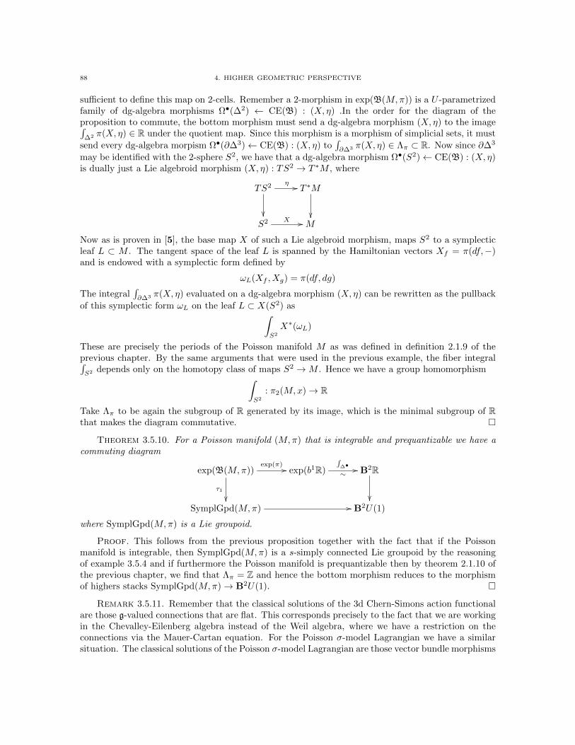
88 4. HIGHER GEOMETRIC PERSPECTIVE
sufficient to define this map on 2-cells. Remember a 2-morphism in exp(B(M,π)) is a U -parametrizedfamily of dg-algebra morphisms Ω•(∆2) ← CE(B) : (X, η) .In the order for the diagram of theproposition to commute, the bottom morphism must send a dg-algebra morphism (X, η) to the image∫
∆2 π(X, η) ∈ R under the quotient map. Since this morphism is a morphism of simplicial sets, it must
send every dg-algebra morpism Ω•(∂∆3)← CE(B) : (X, η) to∫∂∆3 π(X, η) ∈ Λπ ⊂ R. Now since ∂∆3
may be identified with the 2-sphere S2, we have that a dg-algebra morphism Ω•(S2)← CE(B) : (X, η)is dually just a Lie algebroid morphism (X, η) : TS2 → T ∗M , where
TS2
η // T ∗M
S2 X // M
Now as is proven in [5], the base map X of such a Lie algebroid morphism, maps S2 to a symplecticleaf L ⊂ M . The tangent space of the leaf L is spanned by the Hamiltonian vectors Xf = π(df,−)and is endowed with a symplectic form defined by
ωL(Xf , Xg) = π(df, dg)
The integral∫∂∆3 π(X, η) evaluated on a dg-algebra morphism (X, η) can be rewritten as the pullback
of this symplectic form ωL on the leaf L ⊂ X(S2) as∫S2
X∗(ωL)
These are precisely the periods of the Poisson manifold M as was defined in definition 2.1.9 of theprevious chapter. By the same arguments that were used in the previous example, the fiber integral∫S2 depends only on the homotopy class of maps S2 →M . Hence we have a group homomorphism∫
S2
: π2(M,x)→ R
Take Λπ to be again the subgroup of R generated by its image, which is the minimal subgroup of Rthat makes the diagram commutative.
Theorem 3.5.10. For a Poisson manifold (M,π) that is integrable and prequantizable we have acommuting diagram
exp(B(M,π))
τ1
exp(π) // exp(b1R)
∫∆•
∼// B2R
SymplGpd(M,π) // B2U(1)
where SymplGpd(M,π) is a Lie groupoid.
Proof. This follows from the previous proposition together with the fact that if the Poissonmanifold is integrable, then SymplGpd(M,π) is a s-simply connected Lie groupoid by the reasoningof example 3.5.4 and if furthermore the Poisson manifold is prequantizable then by theorem 2.1.10 ofthe previous chapter, we find that Λπ = Z and hence the bottom morphism reduces to the morphismof highers stacks SymplGpd(M,π)→ B2U(1).
Remark 3.5.11. Remember that the classical solutions of the 3d Chern-Simons action functionalare those g-valued connections that are flat. This corresponds precisely to the fact that we are workingin the Chevalley-Eilenberg algebra instead of the Weil algebra, where we have a restriction on theconnections via the Mauer-Cartan equation. For the Poisson σ-model Lagrangian we have a similarsituation. The classical solutions of the Poisson σ-model Lagrangian are those vector bundle morphisms
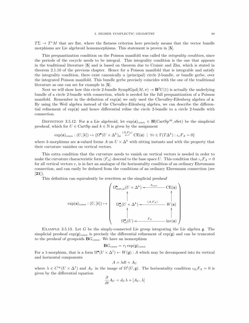
3. HIGHER SYMPLECTIC GEOMETRY 89
TΣ → T ∗M that are flat, where the flatness criterion here precisely means that the vector bundlemorphisms are Lie algebroid homomorphisms. This statement is proven in [5].
This prequantization condition on the Poisson manifold was called the integrality condition, sincethe periods of the cocycle needs to be integral. This integrality condition is the one that appearsin the traditional literature [5] and is based on theorem due to Crainic and Zhu, which is stated intheorem 2.1.10 of the previous chapter. Hence for a Poisson manifold that is integrable and satisfythe integrality condition, there exist canonically a (principal) circle 2-bundle, or bundle gerbe, overthe integrated Poisson manifold. This bundle gerbe precisely coincides with the one of the traditionalliterature as one can see for example in [5].
Next we will show how this circle 2-bundle SymplGpd(M,π)→ B2U(1) is actually the underlyingbundle of a circle 2-bundle with connection, which is needed for the full prequantization of a Poissonmanifold. Remember in the definition of exp(a) we only used the Chevalley-Eilenberg algebra of a.By using the Weil algebra instead of the Chevalley-Eilenberg algebra, we can describe the differen-tial refinement of exp(a) and hence differential refine the circle 2-bundle to a circle 2-bundle withconnection.
Definition 3.5.12. For a a Lie algebroid, let exp(a)conn ∈ H(CartSpop, sSet) be the simplicialpresheaf, which for U ∈ CartSp and k ∈ N is given by the assignment
exp(a)conn : (U, [k]) 7→ Ω•(U ×∆k)si
(A,FA)← CE(a) | ∀v ∈ Γ(T∆k) : ιvFA = 0
where k-morphisms are a-valued forms A on U ×∆k with sitting instants and with the property thattheir curvature vanishes on vertical vectors.
This extra condition that the curvature needs to vanish on vertical vectors is needed in order tomake the curvature characteristic form 〈FA〉 descend to the base space U . This condition that ιvFA = 0for all vertical vectors v, is in fact an analogue of the horizontality condition of an ordinary Ehresmannconnection, and can easily be deduced from the conditions of an ordinary Ehresmann connection (see[21]).
This definition can equivalently be rewritten as the simplicial presheaf
exp(a)conn : (U, [k]) 7→
Ω•vert,si(U ×∆k) CE(a)Avertoo
Ω•si(U ×∆k)
OO
W (a)
OO
(A,FA)oo
Ω•cl(U)
OO
inv(a)
OO
FAoo
Example 3.5.13. Let G be the simply-connected Lie group integrating the Lie algebra g. The
simplicial presheaf exp(g)conn is precisely the differential refinement of exp(g) and can be truncatedto the presheaf of groupoids BGconn. We have an isomorphism
BGconn = τ1 exp(g)conn
For a 1-morphism, that is a form Ω•(U ×∆1)←W (g) : A which may be decomposed into its verticaland horizontal components
A = λdt+AU
where λ ∈ C∞(U × ∆1) and AU in the image of Ω1(U, g). The horizontality condition ι∂tFA = 0 isgiven by the differential equation
∂
∂tAU = dUλ+ [AU , λ]

90 4. HIGHER GEOMETRIC PERSPECTIVE
Take as initial condition AU (t = 0) = A0 then this gives the unique solution
AU (t) = g(t)−1A0g(t) + g(t)−1dUg(t)
where g(t) ∈ G is the parallel transport for the connection λdt along the path [0, t] in the 1-simplex∆1. This is easily seen since
∂
∂tAU (t) = g(t)−1(A0 + dU )λg(t)− g(t)−1λ(A0 + dU )g(t) = dUλ+ [AU (t), λ]
Evaluating this solution at t = 1, and writing g(1) = g and AU (t = 1) = A1 we find
A1 = g−1A0g + g−1dg
which are precisely the gauge transformation between 1-forms A0, A1 ∈ Ω1(U, g). These computationcarry on without substantial modification to higher simplices. The claim then follows from the previousstatement of Lie integration that τ1 exp(g) = BG. Furthermore we the obvious forgetful morpismexp(g)conn → exp(g) can be truncated to the forgetful morphism of stack BGconn → BG.
Example 3.5.14. Let n ≥ 1 and consider the line Lie n-algebra bn−1R. Then fiber integrationover simplices induces an equivalence
∫ conn
∆•: exp(bn−1R)conn → BnRconn
Which is proven in [26].
Remember that for a cocycle µ : a → bn−1R we obtained the morphism of presheaves exp(µ)by postcomposition of k-cells in exp(a) with this cocycle µ. Similarly we can postcompose k-cells inexp(a)conn by postcomposing it with a diagram, which in our case can precisely be done by a diagramof a transgressive cocycle
CE(a) CE(bn−1R)µoo
W (a)
OO
W (bn−1R)
OO
(cs,〈−〉)oo
inv(a)
OO
inv(bn−1R)
OO
〈−〉oo
where 〈−〉 is an invariant polynomial in transgression with the cocycle µ and cs is a Chern-Simonselement witnessing the transgression, which we will also denote by the triple (µ, cs, 〈−〉).
Definition 3.5.15. For every triple (µ, cs, 〈−〉) we can define the morphism of simplicial presheaves
exp(cs) : exp(a)conn → exp(bn−1R)conn
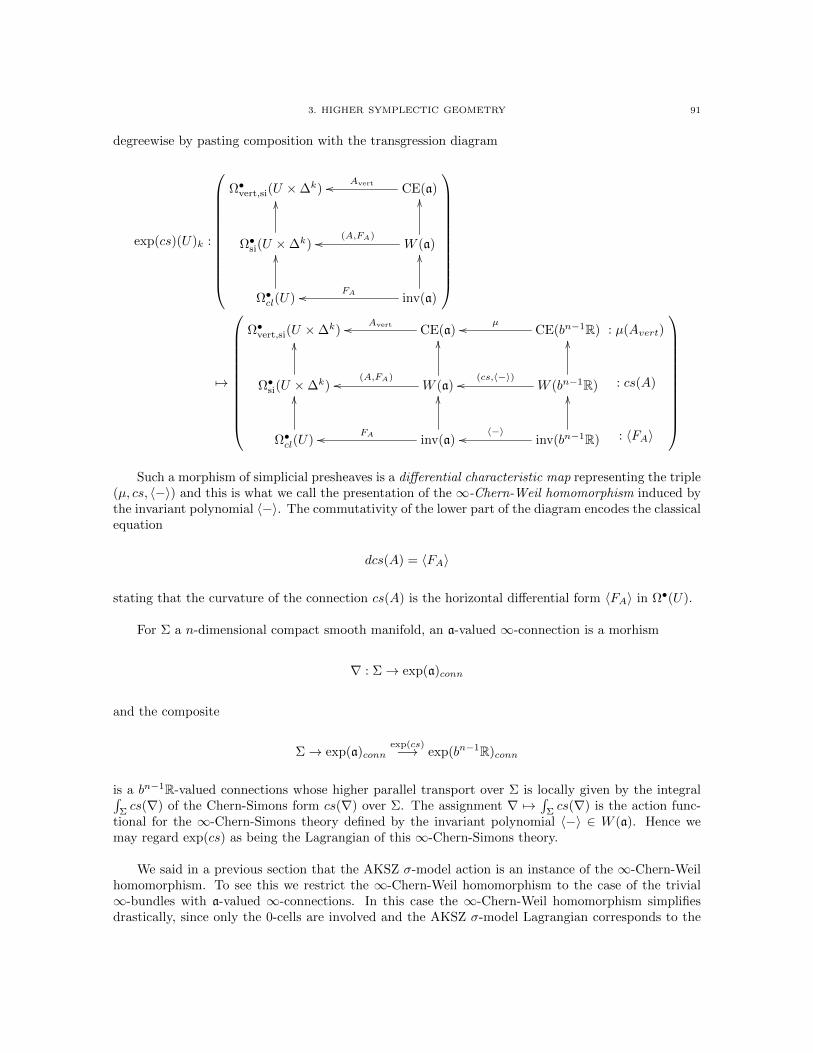
3. HIGHER SYMPLECTIC GEOMETRY 91
degreewise by pasting composition with the transgression diagram
exp(cs)(U)k :
Ω•vert,si(U ×∆k) CE(a)Avertoo
Ω•si(U ×∆k)
OO
W (a)
OO
(A,FA)oo
Ω•cl(U)
OO
inv(a)
OO
FAoo
7→
Ω•vert,si(U ×∆k) CE(a)Avertoo CE(bn−1R)
µoo
Ω•si(U ×∆k)
OO
W (a)
OO
(A,FA)oo W (bn−1R)
OO
(cs,〈−〉)oo
Ω•cl(U)
OO
inv(a)
OO
FAoo inv(bn−1R)
OO
〈−〉oo
: µ(Avert)
: cs(A)
: 〈FA〉
Such a morphism of simplicial presheaves is a differential characteristic map representing the triple
(µ, cs, 〈−〉) and this is what we call the presentation of the ∞-Chern-Weil homomorphism induced bythe invariant polynomial 〈−〉. The commutativity of the lower part of the diagram encodes the classicalequation
dcs(A) = 〈FA〉
stating that the curvature of the connection cs(A) is the horizontal differential form 〈FA〉 in Ω•(U).
For Σ a n-dimensional compact smooth manifold, an a-valued ∞-connection is a morhism
∇ : Σ→ exp(a)conn
and the composite
Σ→ exp(a)connexp(cs)−→ exp(bn−1R)conn
is a bn−1R-valued connections whose higher parallel transport over Σ is locally given by the integral∫Σcs(∇) of the Chern-Simons form cs(∇) over Σ. The assignment ∇ 7→
∫Σcs(∇) is the action func-
tional for the ∞-Chern-Simons theory defined by the invariant polynomial 〈−〉 ∈ W (a). Hence wemay regard exp(cs) as being the Lagrangian of this ∞-Chern-Simons theory.
We said in a previous section that the AKSZ σ-model action is an instance of the ∞-Chern-Weilhomomorphism. To see this we restrict the ∞-Chern-Weil homomorphism to the case of the trivial∞-bundles with a-valued ∞-connections. In this case the ∞-Chern-Weil homomorphism simplifiesdrastically, since only the 0-cells are involved and the AKSZ σ-model Lagrangian corresponds to the

92 4. HIGHER GEOMETRIC PERSPECTIVE
following commutative diagram
Ω•vert,si(U) CE(a)Avertoo CE(bn−1R)
πoo
Ω•si(U)
OO
W (a)
OO
(A,FA)oo W (bn−1R)
OO
(cs,〈−〉)oo
Ω•cl(U)
OO
inv(a)
OO
FAoo inv(bn−1R)
OO
ωoo
: π(Avert)
: cs(A)
: ω(FA)
Example 3.5.16. Consider G a compact simple and simply connected Lie group, with Lie algebrag. Let (b g, 〈−,−〉) be the symplectic Lie 2-algebroid with 〈−,−〉 the Killing form invariant polynomial,transgressing the cocycle µ = − 1
6 〈−, [−,−]〉 via the Chern-Simons element cs ∈ W (b g). We recallthat for a g-valued form Ω•(Σ3)←W (b g) : A this element cs maps to
cs(A) = 〈A ∧ dA〉+1
3〈A ∧ [A ∧A]〉
Now similar to proposition 3.5.8 we have that the triple (µ, cs, 〈−,−〉) defines a commuting diagram
exp(g)conn
τ1
exp(cs)// exp(b2R)conn
∫ conn∆•
∼// B3Rconn
BGconn
c// B3U(1)conn
Where the bottom morphism c : BGconn → B3U(1)conn is the universal characteristic morphism,which is the extended Lagrangian of the 3d Chern-Simons theory. Now take as worldvolume a 3-dimensional closed oriented smooth manifold Σ and consider the mapping stack H(Σ,BGconn) as theconfiguration space, which can be seen as the trajectories of the brane Σ in the target space BGconn.The background gauge field is precisely given by the extended Lagrangian c : BGconn → B3U(1)conn,which can be transgressed to the morphism
H(Σ,BGconn)H(Σ,c)// H(Σ,B3U(1)conn)
exp(2π∫Σ
(−))// U(1)
Since the morphisms in H(Σ,BGconn) are gauge transformations between field configurations, andsince U(1) has no non-trivial morphisms, this map gives necessarily gauge invariant U(1)-valued func-tion on field configurations. Evaluating over the point and passing to equivalence classes, this inducesthe Chern-Simons actions functional
exp(2π
∫Σ
c(−)) : principal G-bundles with connection on Σ/equiv→ U(1)
Now since π3(G) ' H3(G;Z) ' Z we have that the principal G-bundle P → Σ is trivializable andfrom the construction of c we have
exp(2π
∫Σ
c(P,∇)) = exp(2π
∫Σ
cs(A))
where A ∈ Ω1(Σ, g) is the g-valued 1-form on Σ representing the connection ∇ in a chosen trivializationof P . See [29] for more details.

3. HIGHER SYMPLECTIC GEOMETRY 93
This morphism c is the differential refinement of c, and by forgetting the connection we haveobviously the commuting diagram
BGconn
c // B3U(1)conn
BG
c// B3U(1)
which gives precisely the underlying circle 3-bundle of the extended Lagrangian. By forgetting theconnection on both sides of the morphism we loose more information than needed. Actually themorphism c does descend according to the commuting diagram (See [87, 27])
BGconn
c // B3U(1)conn
BG
c// B(B2U(1)conn)
This kind of phenomenon we will see later again.
3.6. 2d Poisson-Chern-Simons theory. Let (M,π) be an integrable Poisson manifold thatsatisfy the integrality condition, and let (B(M,π), ω) be the corresponding symplectic Lie algebroid.In local coordinates the Poisson bivector π = πij∂i ∧ ∂j , the invariant polynomial ω = dxi ∧ d∂i andthe Chern-Simons element that transgresses the cocycle to the invariant polynomial is given by
cs = ∂i ∧ dW (B)xi − π
. Let Σ be a 2-dimensional oriented compact manifold and recall that for a dg-morphism Ω•(Σ) ←W (B) : (X, η) the elements cs maps to
cs(X, η) = η ∧ ddRX +1
2πij(X)ηi ∧ ηj
Which gives the Lagrangian of the Poisson σ-model. The Lie integration of this data gives the extendedLagrangian of an 2d Poisson-Chern-Simons theory. Since similar to proposition 3.5.9 we have that thistriple (π, cs, ω) defines the commuting diagram
exp(B)conn
τ1
exp(cs) // exp(b1R)conn
∫ conn∆•
∼// B2Rconn
SymplGpdconn ∇
// B2U(1)conn
Where SymplGpdconn can be seen as the smooth moduli stack of fields of the 2d Poisson-Chern-Simonstheory and the bottom morphism ∇ : SymplGpdconn → B2U(1)conn is the extended Lagrangian of the2d Poisson-Chern-Simons theory. The non-degenerate and binary invariant polynomial ω, induces byLie integration a pre-2-plectic structure on this moduli stack SymplGpdconn of the 2d Poisson-Chern-Simons theory
ω(F(−), F(−)) : SymplGpdconn → Ω3cl
This curvature morphism we also denote by ω and gives the following prequantization[27]
B2U(1)conn
F(−)
SymplGpdconn
∇66
ω// Ω3cl
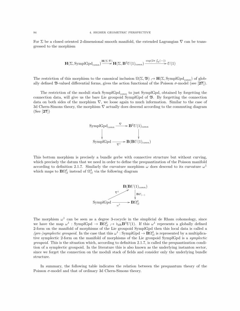
94 4. HIGHER GEOMETRIC PERSPECTIVE
For Σ be a closed oriented 2-dimensional smooth manifold, the extended Lagrangian ∇ can be trans-gressed to the morphism
H(Σ,SymplGpdconn)H(Σ,∇)// H(Σ,B2U(1)conn)
exp(2π∫Σ
(−))// U(1)
The restriction of this morphism to the canonical inclusion Ω(Σ,B) → H(Σ,SymplGpdconn) of glob-ally defined B-valued differential forms, gives the action functional of the Poisson σ-model (see [27]).
The restriction of the moduli stack SymplGpdconn to just SymplGpd, obtained by forgetting theconnection data, will give us the bare Lie groupoid SymplGpd of B. By forgetting the connectiondata on both sides of the morphism ∇, we loose again to much information. Similar to the case of3d Chern-Simons theory, the morphism ∇ actually does descend according to the commuting diagram(See [27])
SymplGpdconn
∇ // B2U(1)conn
SymplGpd
∇1// B(BU(1)conn)
This bottom morphism is precisely a bundle gerbe with connective structure but without curving,which precisely the datum that we need in order to define the prequantization of the Poisson manifoldaccording to definition 2.1.7. Similarly the curvature morphism ω does descend to its curvature ω1
which maps to BΩ2cl instead of Ω3
cl via the following diagram
B(BU(1)conn)
BF(−)
SymplGpd
∇177
ω1// BΩ2
cl
The morphism ω1 can be seen as a degree 3-cocycle in the simplicial de Rham cohomology, sincewe have the map ω1 : SymplGpd → BΩ2
cl → [dRB3U(1). If this ω1 represents a globally defined2-form on the manifold of morphisms of the Lie groupoid SymplGpd then this local data is called a(pre-)symplectic groupoid. In the case that this ω1 : SymplGpd→ BΩ2
cl is represented by a multiplica-tive symplectic 2-form on the manifold of morphisms of the Lie groupoid SymplGpd is a symplecticgroupoid. This is the situation which, according to definition 2.1.7, is called the prequantization condi-tion of a symplectic groupoid. In the literature this is also known as the underlying instanton sector,since we forget the connection on the moduli stack of fields and consider only the underlying bundlestructure.
In summary, the following table indicates the relation between the prequantum theory of thePoisson σ-model and that of ordinary 3d Chern-Simons theory.

3. HIGHER SYMPLECTIC GEOMETRY 95
2d Poisson-Chern-Simonstheory
3d Chern-Simonstheory
Field ConfigurationsB-valued differential form X, η
on a symplectic groupoidg-valued differential form A
on a principal G-bundle(Perturbative) Lagrangian η ∧ ddRX + 1
2πijηi ∧ ηj 〈A ∧ dA〉+ 1
3 〈A ∧ [A ∧A]〉Extended (non-perturbative)
LagrangianSymplGpdconn → B2U(1)conn BGconn → B3U(1)conn
Underlying bundle onthe instanton sector
SymplGpd→ B2U(1)conn1 BG→ B3U(1)conn2
3.7. Boundary field theory. A (codimension 1) boundary theory to a prequantum field theoryL : Fields→ BnU(1)conn is given by a diagram of the form
Fields∂
i
&&yy∗
%%
Fields
LxxBnU(1)conn
t|
That is a choice of boundary fields Fields∂ , a choice of map from boundary fields into bulk fieldsFields, and a choice of trivialization of the extended Lagrangian after restriction to the boundaryfields, see for more details [80, 67]. A famous example of a boundary theory is the Wezz-Zumino-Witten theory as a boundary theory of the 3d Chern-Simons theory. Often these boundary theories oftopological field theories are themselves not topological, but require some extra geometric structure,for example the Wezz-Zumino-Witten theory is a conformal field theory and hence need the choice of aconformal structure. The phenomenon that the bulk fields may be identified with the boundary fieldsin the correlation functions of the boundary theory, is known as the holographic principle. One instanceof the holographic principle in quantum field theory is the relation between the space of quantum statesof 3d Chern-Simons theory may be identified with the correlators of Wezz-Zumino-Witten theory (see[31]).
If we ignore in the above diagram the connection data and write
Fields∂
i∗L
i
%%∗
##
Fields
LyyBnU(1)
ξjr ks
where the right 2-cell is the trivial cell that witness the composition of i and L and the left 2-cellξ is the trivialization of the circle n-bundle i∗L : Fields∂ → BnU(1). The 2-cell ξ that trivializes
the diagram, is in fact a circle (n − 1)-bundle on the boundary fields Fields∂ . This follows from thefact that i∗L is homotopic to the trivial circle n-bundle on M , and morphisms between trivial circlen-bundles are equivalent to circle (n− 1)-bundles.
To see this we first note that the loop space object of the pointed object BnU(1) with point∗ → BnU(1) is equivalent to Bn−1U(1), where the loop space object is defined as the homotopy

96 4. HIGHER GEOMETRIC PERSPECTIVE
pullback ΩBnU(1) of this point along itself
Bn−1U(1) ' ΩBnU(1)
// ∗
∗ // BnU(1)
This follows from the fact that we have the weak equivalence ∗ '→ EBn−1U(1) and the homotopypullback can be computed as an ordinary pullback after replacing one of the morphism by an equivalentfibration
DK(0→ C∞(−, U(1))→ 0 · · · → 0)
// DK(C∞(−, U(1))→ C∞(−, U(1))→ 0 · · · → 0)
DK(0→ 0→ 0 · · · → 0) // DK(C∞(−, U(1))→ 0→ 0 · · · → 0)
which shows that ΩBnU(1) ' Bn−1U(1). Now since i∗L : Fields∂ → BnU(1) is a trivial circlen-bundle it has to factor through the point and by the universal property of the homotopy pullback
Fields∂
ξ
Bn−1U(1)
$$zz∗
$$
∗
zzBnU(1)
we have that ξ : Fields∂ → Bn−1U(1) is a unique circle (n−1)-bundle on the boundary fields. The ex-tended Lagrangian on the bulk fields determines the equation of motion of the fields φ : Σn → Fields,where Σn can be seen as as a n-dimensional closed oriented manifold that propagates through thetarget space Fields. If Σn has a boundary ∂Σn such that φ(∂Σn) ⊆ Fields∂ , then the equation ofmotion of the boundary fields is determined by the extended Lagrangian on the boundary, which isprecisely given by this circle (n− 1)-bundle ξ : Fields∂ → Bn−1U(1).
The extended Lagrangian of the 2d Poisson-Chern-Simons theory given by the prequantum circle2-bundle ∇1 can be interpreted in these terms. Notice that the integration of the Poisson manifoldM also gave us the inclusion i : M → SymplGpd, which we call the atlas. The pullback of thisprequantum circle 2-bundle ∇1 along this atlas gives the following trivialization
M
i
((yy∗
$$
SymplGpd
∇1wwB2U(1)conn1
s

4. HIGHER GEOMETRIC QUANTIZATION 97
Which means that the pullback of the underlying circle 2-bundle is trivializable, and that the cor-responding 2-connection is trivial. To see this remember that ∇1 can be described by a line bundleL over the manifold of morphisms of SymplGpd together with a connection ∇ and a cocycle σ thathas norm 1 and which is compatible with the connection. The cocycle σ makes the pullback i∗L overM into a trivial line bundle over M . Hence there exist a unit section of i∗L over M , and since σ iscompatible with the connection this unit section has to be covariantly constant from which it followsthat the connection has to be trivial.
The instanton sector SymplGpd can be seen as the phase space of the open string 2d Poisson-Chern-Simons theory. An open string moving in SymplGpd can have some of its endpoints confinedto the boundary M . These confined endpoints are forced to move inside the boundary M , which inthe physics literature is also called a D-brane. These endpoints behave as particles moving in M . Themotion of these open strings in SymplGpd are determined by the equation of motion of the actionfunctional of the extended Lagrangian ∇1. By the above this extended Lagrangian ∇1 also give acircle bundle on ξ on M , which in particular determines the equation of motion of the particles thatmove in M . In this way, the geometric quantization procedure of Hawkins[39] secretly quantizes notonly the Poisson manifold with its prequantum circle bundle, but als the 2d Poisson-Chern-Simonstheory with its prequantum circle 2-bundle.
Remark 3.7.1. This point of view was already suggested by Cattaneo and Felder [8], where theystudied the Poisson σ-model via the Hamiltonian formalism. They constructed a canonical momentmap via which the symplectic groupoid as the phase space of the Poisson σ-model is obtained bysymplectic reduction.
4. Higher geometric quantization
The geometric quantization of the prequantum circle 2-bundle ∇1 over the symplectic groupoid,was done by interpreting ∇1 as the multiplicative prequantum line bundle over the space of morphismsof the symplectic groupoid. We constructed the convolution C∗-algebra A(∇0) of sections of theunderlying multiplicative prequantum line bundle ∇0 (tensored with half-densities) and we consideredthe subalgebra
A(∇0)P → A(∇0)
of polarized sections, after choosing a suitable polarization. This convolution subalgebra of the pre-quantum circle 2-bundle ∇1 can naturally be interpreted in higher geometry by considering bundlegerbe modules.
For every ordinary central extension of Lie groups U(1)→ U(n)→ PU(n) we have the delooping
sequence BU(1) → BU(n) → BPU(n)ddn→ B2U(1), where the last map is the universal Dixmier-
Douady class of smooth PU(n)-principal bundles (see [27]). For ∇0 : SymplGpd → B2U(1) theunderlying bundle of ∇1, a section σ of the associated BU(n)-fiber 2-bundle is a dashed lift
BPU(n) ' BU(n)//BU(1)
ddn
SymplGpd
σ
55
∇0// B2U(1)
The lift σ of the bundle gerbe ∇0 is equivalent to what is called a bundle gerbe module or rank n twistedunitary bundle. These sections σ, as ∇0-twisted unitary bundles, are equivalent to the (pre-)quantum2-states of ∇1 regarded as a prequantum 2-bundle (see [11]). By section 5 of [11], we find that a bundlegerbe module of the bundle gerbe ∇0 is precisely a module over C∗-algebra A(∇0)P . These modulesover A(∇0)P form together the category ModA(∇0)P of modules, which can be interpreted as a 2-vector

98 4. HIGHER GEOMETRIC PERSPECTIVE
space. Notice that the category of k-vector spaces is the category of k-modules Vectk = k-Mod andthe 2-category of 2-vector spaces is
2Vect = VectVect = Vect-Mod
that is the 2-category of abelian categories equipped with a (Vect,⊗)-action. The strict 2-categoryof Algebras of algebras, algebra homomorphisms and intertwiners (that is the 2-category for algebrasregarded as one-object Vect-enriched categories) are sitting inside 2Vect according to (see appendix of[81])
Algebras // 2Vect
A
N
N ′
BBBφ
7→ ModA
−⊗AN
−⊗AN ′
>>ModB−⊗Aφ
Hence the quantum 2-states of the prequantum 2-bundle ∇1, that are the ∇0-twisted unitary bundlesare naturally interpreted as an instance of a 2-vector space
quantum 2-states ofprequantum 2d Poisson-Chern-Simons theory
' ModA(∇0)P ∈ 2Vect
In this way the geometric quantization of the Poisson manifold M can be seen as the higher geomet-ric quantization of the 2d Poisson-Chern-Simons theory. We can think of the Poisson manifold as aquantum mechanical system, hence a 1-dimensional quantum field theory, which in the case it is asymplectic manifold yields a vector space of quantum states. Where similarly the higher geometricquantization of the 2d Poisson-Chern-Simons theory yields a 2-vector space of quantum 2-states. Thisindicates a holographic relation between higher geometric quantization of the 2d Poisson-Chern-Simonstheory and quantum mechanics as a 1d quantum field theory.
These category of modules ModA(∇0)P can naturally be interpreted as 2-vector spaces with a 2-basis. Just like an ordinary k-vector space V has as basis a set S such that V ' HomSet(S, k), a2-basis for a 2-vector space V has to be a category S such that V ' Hom(S,Vect). If S is a Vect-enriched category and we see Vect as a Vect-enriched over itself, then V ' Hom(S,Vect) correspondsto the Vect-enriched functors from S to Vect. A Vect-enriched category S is just a linear category (oralgebroid) and if it has a single object it is an algebra and we have
ModA(∇0)P = Hom(BA(∇0)P ,Vect)
where the algebra A(∇0)P is here regarded as the one-object Vect-enriched category BA(∇0)P . Hencethe linear category BA(∇0)P can be regarded as the 2-basis of the 2-vector space ModA(∇0)P . In this
sense the we can interpreted the algebra A(∇0)P in higher geometry as the 2-basis for the 2-space ofquantum 2-states.
From the point of view of ordinary geometric quantization, we produced a space of states from thespace of sections of the prequantum bundle, and the constructions of the algebra of operators actingon this space of states required some work. From the point of view of the geometric quantizationor strict C∗-deformation quantization of Hawkins[39], we produced immediately the algebra. The 2-space of 2-states we got from taking sections of the associated BU(n)-fiber 2-bundle associated to theprequantum 2-bundle, which has the algebra as 2-basis. The construction of the 2-algebra of higheroperators acting on these 2-states is still an open question.
This strict C∗-deformation quantization approach of Hawkins[39] has a infinitesimal analogue,which is the formal deformation quantization of the Poisson manifold, which was studied by Konstevich,
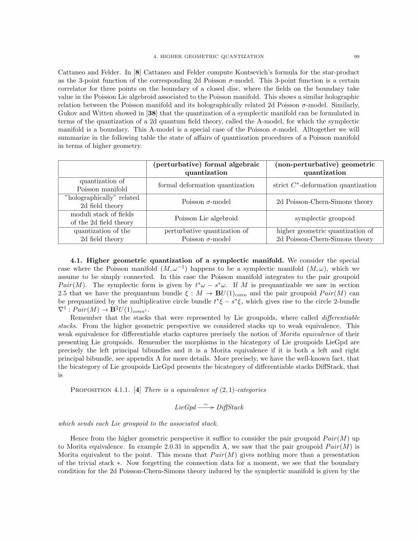
4. HIGHER GEOMETRIC QUANTIZATION 99
Cattaneo and Felder. In [8] Cattaneo and Felder compute Kontsevich’s formula for the star-productas the 3-point function of the corresponding 2d Poisson σ-model. This 3-point function is a certaincorrelator for three points on the boundary of a closed disc, where the fields on the boundary takevalue in the Poisson Lie algebroid associated to the Poisson manifold. This shows a similar holographicrelation between the Poisson manifold and its holographically related 2d Poisson σ-model. Similarly,Gukov and Witten showed in [38] that the quantization of a symplectic manifold can be formulated interms of the quantization of a 2d quantum field theory, called the A-model, for which the symplecticmanifold is a boundary. This A-model is a special case of the Poisson σ-model. Alltogether we willsummarize in the following table the state of affairs of quantization procedures of a Poisson manifoldin terms of higher geometry.
(perturbative) formal algebraicquantization
(non-perturbative) geometricquantization
quantization ofPoisson manifold
formal deformation quantization strict C∗-deformation quantization
”holographically” related2d field theory
Poisson σ-model 2d Poisson-Chern-Simons theory
moduli stack of fieldsof the 2d field theory
Poisson Lie algebroid symplectic groupoid
quantization of the2d field theory
perturbative quantization ofPoisson σ-model
higher geometric quantization of2d Poisson-Chern-Simons theory
4.1. Higher geometric quantization of a symplectic manifold. We consider the specialcase where the Poisson manifold (M,ω−1) happens to be a symplectic manifold (M,ω), which weassume to be simply connected. In this case the Poisson manifold integrates to the pair groupoidPair(M). The symplectic form is given by t∗ω − s∗ω. If M is prequantizable we saw in section2.5 that we have the prequantum bundle ξ : M → BU(1)conn and the pair groupoid Pair(M) canbe prequantized by the multiplicative circle bundle t∗ξ − s∗ξ, which gives rise to the circle 2-bundle∇1 : Pair(M)→ B2U(1)conn1 .
Remember that the stacks that were represented by Lie groupoids, where called differentiablestacks. From the higher geometric perspective we considered stacks up to weak equivalence. Thisweak equivalence for differentiable stacks captures precisely the notion of Morita equivalence of theirpresenting Lie groupoids. Remember the morphisms in the bicategory of Lie groupoids LieGpd areprecisely the left principal bibundles and it is a Morita equivalence if it is both a left and rightprincipal bibundle, see appendix A for more details. More precisely, we have the well-known fact, thatthe bicategory of Lie groupoids LieGpd presents the bicategory of differentiable stacks DiffStack, thatis
Proposition 4.1.1. [4] There is a equivalence of (2, 1)-categories
LieGpd∼ // DiffStack
which sends each Lie groupoid to the associated stack.
Hence from the higher geometric perspective it suffice to consider the pair groupoid Pair(M) upto Morita equivalence. In example 2.0.31 in appendix A, we saw that the pair groupoid Pair(M) isMorita equivalent to the point. This means that Pair(M) gives nothing more than a presentationof the trivial stack ∗. Now forgetting the connection data for a moment, we see that the boundarycondition for the 2d Poisson-Chern-Simons theory induced by the symplectic manifold is given by the

100 4. HIGHER GEOMETRIC PERSPECTIVE
diagram
M
i
''||∗
""
Pair(M) ' ∗
∇0xxB2U(1)
ξt|
Where we immediately see that ξ is given by the unique map to the loop space object of B2U(1), thatis
M
ξ
BU(1)
##∗
##
∗
B2U(1)
and so is equivalent to the prequantum circle bundle ξ : M → BU(1). Remember from the exampleof section 8.1, that the strict C∗-deformation quantization of a symplectic manifold together with acertain polarization P is taken to be the C∗-algebra of compact operators on the leaf space M/P . Wefound that the C∗-algebra of compact operators is the twisted polarized convolution algebra of the thesymplectic groupoid Pair(M/P ) carrying a circle 2-bundle. The fact that we consider Lie groupoids upto Morita equivalence is also reflected in their associated convolution algebras. In [50, 52] Landsmanproved that Morita equivalent Lie groupoids have Morita equivalent convolution algebras. Hence theMorita equivalence of the pair groupoid Pair(M/P ) and the point ∗ is reflected by the well-knownfact that the compact operators are Morita equivalent to the base algebra of complex numbers.
In this sense Hawkins’ strict C∗-deformation quantization is not Morita faithful, meaning that itdistinguishes Morita equivalent Lie groupoids and Morita equivalent C∗-algebras. The above exampleshows us that Hawkins’ solution of the strict C∗-deformation problem does not have intrinsic meaningunder Morita equivalence, since for the symplectic manifold case, one just arrives at a trivial quan-tization. Hence in this higher geometric perspective Hawkins’ strict C∗-deformation quantization ofsymplectic manifolds contains a conundrum: either one breaks with the Morita equivalence or else onearrives at trivial quantization.

CHAPTER 5
Outlook
In the previous chapter we saw that in the higher geometric perspective Hawkins’ strict C∗-deformation quantization of symplectic manifolds contains a conundrum, that is either one breakswith the Morita equivalence or else one arrives at trivial quantization. This conundrum is resolvedby quantizing more than just the symplectic groupoid itself. From the Lie groupoid perspectiveone sees that the convolution algebra is only sensitive to the underlying differentiable stack and theinformation missing in the latter is precisely the induced atlas, given by the epimorphism of smoothstacks M → SymplGpd, which is given by the inclusion of the manifold of objects into the Lie groupoid.Together with the trivial stack ∗ as terminal object, this is equivalent to the datum of a correspondence
∗ Mi //oo SymplGpd
which exhibits the original as a boundary of the corresponding 2d Chern-Simons theory if there existsa lift to the prequantum field theory given by the diagram
M
i
&&∗
""
SymplGpd
∇0xxB2U(1)
ξu
We do not only assign to the differentiable stack SymplGpd carrying a circle 2-bundle SymplGpd →B2U(1) a twisted convolution algebra as a C∗-algebra, but we can assign to a morphism of differentiablestacks carrying circle 2-bundles a Hilbert bimodule of C∗-algebras. In [67] Nuiten shows that forminggroupoid twisted convolution algebras naturally extends to a functor of (2,1)-categories
(DiffStacksprop)op/B2U(1)
C∗(−) // C∗Algprop
from differentiable stacks over B2U(1) to C∗-algebras with (proper) Hilbert bimodules between them.Appyling this functor to the above span of differentiable stacks over B2U(1) gives us a co-span ofHilbert bimodules
Cξ // C∗i∗∇0(M) C∗∇0(SymplGpd)
i∗oo
These are Hilbert bimodules of twisted convolution algebras and for Hawkins’ strict C∗-deformationquantization we needed a twisted polarized convolution algebra, which were constructed from a con-nection on the circle 2-bundles over the groupoid together with the choice of a certain polarizition. Inthe symplectic manifold case, this connection and polarization were induced from the connection andpolarization of its traditional geometric quantization scheme via polarization. But remember that fortraditional geometric quantization of symplectic manifolds, we also had the Spinc-geometric quanti-zation scheme. In this quantization scheme we only needed to choose a Spinc-structrure such that itsassociated determinant line bundle is a prequantum line bundle. The actual Spinc-quantization was
101

102 5. OUTLOOK
the index of its corresponding Spinc-Dirac operator. This index is precisely described by a pushforwardmap in K-theory, which was already observed by [61].
The description of maps in K-theory via elliptic operators is nicely captured in KK-theory, whichis a bivariant generalization of operator K-theory and K-homology. The KK-groups in KK-theory arenatural homotopy equivalence classes of Hilbert bimodules equipped with some Fredholm operator andthe famous Kasparov product gives the composition operation between these KK-groups and henceinduces the KK-category. Furthermore there is a natural functor
C∗Algprop // KK
from the bicategory of C∗-algebras with (proper) bimodules to the category KK. Hence the abovecospan of Hilbert bimodules can be regarded as a cospan in KK-theory. And in order to push-forwardin K-theory we need to turn the right map around, that is instead of pulling back along the map i, wepush along it. For the full construction we refer the reader to [67], but we will give here the main idea.We begin by noting that the choice of Spinc-structure in Spinc-quantization, precisely corresponds toa choice of what is called a K-orientation of the atlas, which is in our case the inclusion map i. Thischoice of Spinc-structure does only not restrict to symplectic manifold and in our case can be definedfor any compact Poisson manifold M . Assuming that C∗∇0
(SymplGpd) is dualizable in KK then wehave a canonical dual map
(i∗)∨ : C∗i∗∇0(M)∨ // C∗∇0
(SymplGpd)∨
The choice of a K-orientation determines a Thom isomorphism
Th(M) : C∗i∗∇0(M) // C∗i∗∇0
(M)∨
and composing these two maps gives what is called the Umkehr map
i! : C∗i∗∇0(M)
Th // C∗i∗∇0(M)∨
(i∗)∨ // C∗∇0(SymplGpd)∨
Now the pull-push quantization in KK-theory is given by the composition
Cξ // C∗i∗∇0
(M)i! // C∗∇0
(SymplGpd)∨ ∈ KK(C, C∗∇0(SymplGpd)∨) = K0(C∗∇0
(SymplGpd)∨)
Which describes precisely a K-theory class of C∗∇0(SymplGpd)∨. Notice that the symplectic groupoid
SymplGpd of a Poisson manifold behaves roughly like the symplectic leaf space of the Poisson manifold.In particular if the Poisson manifold happens to be a symplectic manifold, then the symplectic groupoidis equivalent to the point. In this case the above yields an element of the K-theory of the point and asis proven in [67] we get precisely the traditional Spinc-quantization for symplectic manifolds, that isi!(L) = index(DL) ∈ KK(C,C) ∈ Z, where L is here ξ. In this sense a class in K0(C∗∇0
(SymplGpd)∨)may be thought of as providing one (virtual) vector space for each symplectic leaf, to be thougth of asthe space of quantum states.
That KK-theory is a natural codomain for quantization of Poisson manifolds has long been ampli-fied by Landsman[53], but Landsman focused mainly on the issue of symplectic reduction, while herethe point is to define the quantization of Poisson manifolds. This pull-push quantization thought ofas a 2-geometric quantization of Poisson manifolds should fix the issue that the strict C∗-deformationquantization of Hakwins is not Morita faithful.
The general framework for pull-push quantization is treated in [67] where several other applica-tions are covered. For example the extension of geometric quantization of symplectic manifold thatcarry a Hamiltonian G-action by pushing forward in equivariant K-theory, the D-brane charges as thequantization of a particle at the boundary of a string, the M9-brane charge as the quantization of astring moving at the boundary of a 2-brane, to name a few. This pull-push quantization is a first step

5. OUTLOOK 103
in the direction of a full description of geometric quantization for every prequantum field theory. Weonly treated the case where we lifted a correspondence of the form
∗ Mi //oo SymplGpd
to a diagram
M
i
&&∗
""
SymplGpd
xxB2U(1)
u
But in the full n-dimensional prequantum field theory we want to consider more generally any n-foldcorrespondence by a monoidal functor
BordnFields // Corrn(H)
from the (∞, n)-category of cobordisms to the (∞, n)-category of n-fold correspondences in H and anaction functional on this field as a lift of monoidal functors
Corrn(H/BnU(1))
Bordn
exp(iS)77
Fields // Corrn(H)
where the morphism exp(iS) maps to n-fold correspondences in the slice topos over the moduli stack ofcircle n-bundles. This datum together is called a n-dimensional prequantum field theory (see [80, 67]).We have only treated the quantization of a single correspondence diagram of the above specific form. Asingle correspondence diagram of a more general form is treated in [67]. Since the n-fold correspondencediagrams are built up from single spans, one hopes that this is a first step in right direction for thequantization of n-fold correspondences. Furthermore the pull-push quantization works mainly for thecase where one considers spans of differentiable stacks over B2U(1), where one can apply the twisted K-theory for differentiable stacks. But for arbitrary stacks over BnU(1) there is still no general procedure.The well-understood geometric quantization of 3d Chern-Simons theory should at least give a blueprintfor the case n = 3. Eventually one would like to have a fully extended geometric quantization of allprequantum field theories, but this requires still some work.

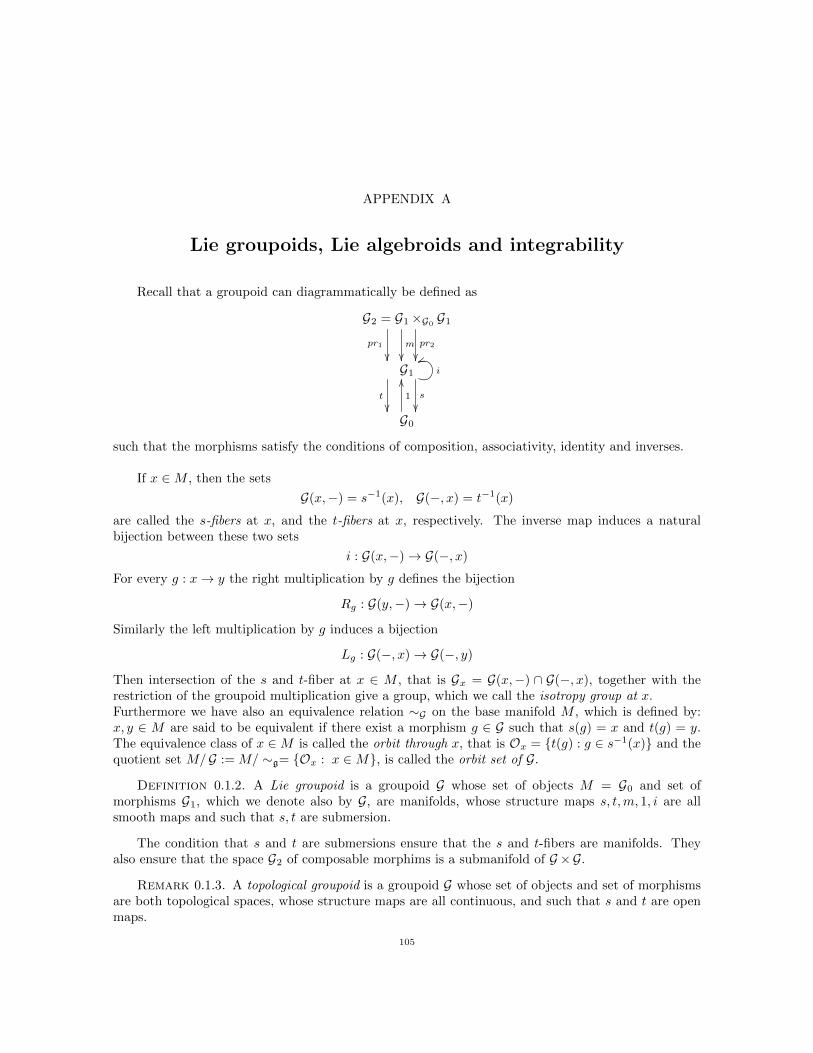
APPENDIX A
Lie groupoids, Lie algebroids and integrability
Recall that a groupoid can diagrammatically be defined as
G2 = G1×G0G1
pr2
m
pr1
G1 ivv
s
t
G0
1
OO
such that the morphisms satisfy the conditions of composition, associativity, identity and inverses.
If x ∈M , then the sets
G(x,−) = s−1(x), G(−, x) = t−1(x)
are called the s-fibers at x, and the t-fibers at x, respectively. The inverse map induces a naturalbijection between these two sets
i : G(x,−)→ G(−, x)
For every g : x→ y the right multiplication by g defines the bijection
Rg : G(y,−)→ G(x,−)
Similarly the left multiplication by g induces a bijection
Lg : G(−, x)→ G(−, y)
Then intersection of the s and t-fiber at x ∈ M , that is Gx = G(x,−) ∩ G(−, x), together with therestriction of the groupoid multiplication give a group, which we call the isotropy group at x.Furthermore we have also an equivalence relation ∼G on the base manifold M , which is defined by:x, y ∈ M are said to be equivalent if there exist a morphism g ∈ G such that s(g) = x and t(g) = y.The equivalence class of x ∈M is called the orbit through x, that is Ox = t(g) : g ∈ s−1(x) and thequotient set M/G := M/ ∼g= Ox : x ∈M, is called the orbit set of G.
Definition 0.1.2. A Lie groupoid is a groupoid G whose set of objects M = G0 and set ofmorphisms G1, which we denote also by G, are manifolds, whose structure maps s, t,m, 1, i are allsmooth maps and such that s, t are submersion.
The condition that s and t are submersions ensure that the s and t-fibers are manifolds. Theyalso ensure that the space G2 of composable morphims is a submanifold of G ×G.
Remark 0.1.3. A topological groupoid is a groupoid G whose set of objects and set of morphismsare both topological spaces, whose structure maps are all continuous, and such that s and t are openmaps.
105

106 A. LIE GROUPOIDS, LIE ALGEBROIDS AND INTEGRABILITY
We call G s-connected if the s-fibers are connected, G is called s-simply connected if they are simplyconnected and G is called s-locally trivial if they form a bundle. Any Lie groupoid G has an associateds-connected groupoid G0, the s-connected component of the identities.
A morphism between two Lie groupoids G over M and H over N is a morphism between groupoids,i.e. it consists of a map F : G → H between the set of arrows and a map f : M → N between the set ofobjects, which are compatible with all the structure maps, and in addition these two morphism needsto be smooth. The Lie groupoids together with there morphisms form the category of Lie groupoids.
A Lie subgroupoid of a groupoid G is a pair (H, i), where H is a groupoid and i : H → G is aninjective immersive groupoid morphism. A wide Lie subgoupoid is a Lie subgroupoid H ⊂ G which hasthe same space of units as G.
Let F : G → H, f : M → N be a morphism of groupoids. Then the kernel of F is the setker(F ) := g ∈ G : F (g) = 1(x), ∃x ∈ N.
Example 0.1.4. (Groups) A group is nothing more then a groupoid for which the set of objectscontains a single element. Obviously Lie groups are examples of Lie groupoids.
Example 0.1.5. (The pair groupoid) Let M be any set. The Cartesian product Pair(M) := M ×M is the pair groupoid over M where the set of objects is M and where we take a pair (x, y) ∈M ×Mas a morphism x→ y. Composition is defined by:
(z, y) (y, x) = (z, x)
If M is a manifold, then the pair groupoid is a Lie groupoid.
Example 0.1.6. (The fundamental groupoid) Let M be a manifold. The fundamental groupoid ofM , denoted by Π1(M) is the groupoid whose set of objects is M and whose morphisms from x to y arethe homotopy classes [γ] of continuous maps γ : [0, 1]→M with γ(0) = 1 and γ(1) = y. Compositionis defined by concatenation and reparametrization of representative maps. The homotopy-equivalencerelation makes it a groupoid. Note also that, when M is connected and simply-connected, Π1(M) isisomorphic to the pair groupoid Pair(M), since a homotopy class of a path is determined by its endpoints. In general the fundamental groupoid Π1(M) is the connected cover of Pair(M).
Example 0.1.7. (The gauge groupoid) Let G be a Lie group and π : P → M be a left principalG-bundle. Remember that a smooth map of principal G-bundle φ : P → P that commutes with theG-action is called a gauge transformation. Then we define Gauge(P ) to be the gauge groupoid thatis the groupoid P ×G P over M , where P ×G P is the orbit space of the diagonal action of G onP × P . It obtains a groupoid structure from the pair groupoid Pair(P ) over P , that is s := π pr2,t := π pr1 and composition is given by [p, q][q′, r] = [p, q][q, g · r] = [p, g · r] where p, q, q′, r ∈ P suchthat π(q) = π(q′) and g ∈ G is unique such that g · q′ = q. The unit is defined by 1(x) =: [p, p] for anyp ∈ π−1(x) and the inverse is given by [p, q]−1 := [q, p] for p, q ∈ P .
We saw that a Lie groupoid is a generalization of a Lie group, and we know that the infinitesimalobjects corresponding to a Lie group is a Lie algebra. Now similarly the infinitesimal object thatcorrespond to a Lie groupoid is a Lie algebroid. A Lie algebra consists of a vector space that correspondsto the tangent space of the group at the unit element, hence we expect that a Lie algebroid is a vectorbundle over M , since we have a unit for each point in M . Secondly the vector space of a Lie algebracan be identified with the space of left invariant vector field on the group and this space of left invariantvector fields is closed under the Lie bracket of vector fields. Now since left multiplication on a Liegroupoid G is only defined on the t-fibers, the left invariant vector fields on G should be those vectorfields which are tangent to the t-fibers, i.e. the sections of the subbundle T t G of T G defined by
T t G = ker(dt) ⊂ T GHence the corresponding vector bundle A of a G should have for each fiber at x ∈M the tangent spaceat the unit of the t-fiber at x, i.e. A := T t G |M . It turns out the there exists here also an isomorphism
A. LIE GROUPOIDS, LIE ALGEBROIDS AND INTEGRABILITY 107
between the space of left invariant vector fields and the space of sections of A, which we denote byΓ(A). The Lie bracket [·, ·])A on A is the Lie bracket on Γ(A) obtained from the Lie bracket on thespace of left invariant vector fields under this isomorphism. To describe the entire structure underlyingA we need also an anchor map of A, which is a bundle map ρA : A → TM obtained by restrictingds : T G → TM to A ⊂ T G. This defined Lie bracket and anchor map are related by the Leibnizidentity. Let α, β ∈ Γ(A) and f ∈ C∞(M), then
[α, fβ]A = f [α, β]A + ρA(α)(f)β
For more details we refer the reader to [16]. Summarizing the above gives us the following definition:
Definition 0.1.8. The Lie algebroid of the Lie groupoid G is the vector bundle A := T t G |M ,together with the anchor ρA : A→ TM and the Lie bracket on [·, ·]A on Γ(A).
Proposition 0.1.9. For any Lie groupoid, G0 is an open subgroupoid of G. Hence, G0 is thes-connected Lie groupoid that has the same Lie algebroid as G.
We arrive at the abstract notion of a Lie algebroid:
Definition 0.1.10. A Lie algebroid over a manifold M consists of a vector bundle A together witha bundle map ρA : A→ TM , called the anchor map, and a Lie bracket [·, ·]A on the space of sectionsΓ(A), satisfying the Leibniz identity:
[α, fβ]A = f [α, β]A + ρA(α)(f)β
for α, β ∈ Γ(A) and f ∈ C∞(M).
A morphism between two Lie algebroids A1 →M1 and A2 →M2 is a vector bundle map
A1
F // A2
M1
f// M2
which is compatible with the anchors, that is
df(ρA1(a)) = ρA2(F (a))
and is compatible with the Lie bracket, that is
F ([α, β]A1) = [α′, β′]A2 f
for α, β ∈ Γ(A1) and where α′, β′ ∈ Γ(A2) are defined by F (α) = α′ f and F (β) = β′ f .The Lie algebroids together with there morphisms form the category of Lie algebroids. Every
morphism of Lie groupoids induce a morphism between their associated Lie algebras, hence thereexists a Lie functor A from the category of Lie groupoids to the category of Lie algebroids (see [58]).
Example 0.1.11. (Lie algebras) Any Lie algebra g is a Lie algebroid over the singleton. The abovefunctor A restricts to the classical functor from Lie groups to Lie algebras.
Example 0.1.12. (Tangent bundles) The tangent bundle A = TM is an example of a Lie algebroid,with the identity map as anchor, and the usual Lie bracket of vector fields.
Example 0.1.13. (Poisson manifolds) Let M be a manifold. The space of smooth functions on M ,denoted by C∞(M) is a vector space and forms an algebra by pointwise multiplication of functions. APoisson bracket on a manifold M is a Lie bracket ·, · on the algebra C∞(M) satisfying the derivationproperty:
fg, h = ff, h+ gf, h ∀f, g, h ∈ C∞(M)
108 A. LIE GROUPOIDS, LIE ALGEBROIDS AND INTEGRABILITY
We call the algebra C∞(M) together with the Poisson bracket ·, · a Poisson algebra, which we denoteby (C∞(M), ·, ·). A Poisson manifold is a manifold M equipped with a Poisson bracket ·, · on thealgebra C∞(M) such that (C∞(M), ·, ·) is a Poisson algebra. We call this Poisson algebra also thePoisson structure on M . Alternatively a Poisson structure on a manifold M is given by a choice ofsmooth antisymmetric bivector, called a Poisson bivector, π ∈ Γ(∧2TM) such that
f, gπ = π(df, dg)
and ·, ·π satisfy Jacobi identity. Let π be a Poisson bivector on a manifold M . This Poisson structureinduces a Lie algebroid structure on T ∗M as follows. Define the map
π] : T ∗M → TM
by β(π](α)) = π(α, β). The Lie algebroid structure on T ∗M has π] as anchor map, and the Lie bracket,also called the Koszul bracket, is defined by
[α, β] = Lπ](α)(β)− Lπ](β)(α)− d(π(α, β))
We call this the Poisson Lie algebroid of the Poisson manifold (M,π).
We saw that any Lie groupoid has an associated Lie algebroid.
Definition 0.1.14. A Lie algebroid A is called integrable if it is isomorphic to the Lie algebroidof a Lie groupoid G. For such a G, we say that G integrates A.
We introduce this definition since not every Lie algebroid is integrable, the obstructions to integratea Lie algebroid are discussed in detail in [17]. Suppose A is a Lie algebroid over M , then we canconstruct a topological groupoid G(A). It turns out that whenever A is integrable, this topologicalgroupoid G(A) admits smooth structure, which makes it a Lie groupoid, such that it integrates A. Themain idea is as follows: Suppose π : A→ M is an integrable Lie algebroid. Define an A-path a to bea curve a : [0, 1] → A with the property that ρA(a(t)) = d
dtπ(a(t)). Denote by P (A) the space of A-paths. We can compose two A-paths if they have the same end-points. In order for these compositionto be smooth we need to introduce some cut-off function and reparametrization which defines themultiplication of composable A-paths. Under the equivalence relation of homotopy of A-paths we canconstruct our groupoid G(A) as G(A) = P (A)/ ∼, which is called the Weinstein groupoid.
Theorem 0.1.15. If A is integrable, then there exists an unique (up to isomorphism) s-simplyconnected Lie groupoid G(A) integrating A.
Theorem 0.1.16. Let φ : A → B be a morpism of integrable Lie algebroids, and let G(A) andH(B) be integrations of A and B. If G(A) is s-simply connected, then there exists a (unique) morphismof Lie groupoids Φ : G(A)→ H(H) integrating φ.
Hence there exists an inverse functor G of A, which has as domain the full subcategory of integrableLie algebroids. For more details see [17].
Remark 0.1.17. The notion of integrability does not include the assumption of Hausdorfness. Inthe theory of Lie groupoids, it is often necessary to consider non-Hausdorff groupoids. We will assumethat the base manifold, algebroids, and the s- and t-fibers are Hausdorff. The non-Huasdorff case willnot be addressed in this thesis.
1. Poisson Geometry
We are especially interested in the integration of Poisson manifolds, since a Lie algebroid integratinga Poisson manifold has a natural symplectic structure, which will be usefull for developing variousquantization schemes.
1. POISSON GEOMETRY 109
Definition 1.0.18. Let G be a Lie groupoid and ω ∈ Ω∗(G1). Let ∂∗ω := pr∗1ω −m∗ω + pr∗2ω,then we call ω multiplicative if
∂∗ω = 0
A symplectic groupoid is a groupoid Σ with a multiplicative symplectic form ω ∈ Ω2(Σ1).
Remark 1.0.19. The nerve G∗ of a groupoid G has a natural structure of a simplicial manifold. Thisstructure gives a boundary operator ∂∗ on differential forms on the double complex Ω∗(G∗), which is thesimplicial de Rham complex of the nerve G∗. That is for θ ∈ Ω∗(M) we have ∂∗θ := t∗θ− s∗θ ∈ Ω∗(G)and for ω ∈ Ω∗(G) we have ∂∗ω := pr∗1ω −m∗ω + pr∗2ω ∈ Ω∗(G2). The simplicial coboundary extendsto line bundle, since for a line bundle L over M we have the line bundle ∂∗L := t∗L ⊗ s∗L∗ overG. Similarly a line bundle L over G gives a line bundle ∂∗L := pr∗1L ⊗m∗L∗ ⊗ pr∗2L over G2, whichcontinuous this way for higher Gk. The coboundary of a coboundary, that is ∂∗∂∗L is canonically atrivial line bundle, since curv ∂∗∂∗L = ∂∗∂∗(curv L). A section of a line bundle σ ∈ Γ(Gk, L) has amultiplicative coboundary ∂∗σ ∈ Γ(Gk, ∂∗L).
The base manifold of a symplectic groupoid has a canonical Poisson bracket.
Proposition 1.0.20. Let (Σ, ω) be a symplectic groupoid over M . Then there exists a uniquePoisson structure on M such that s is Poisson and t is anti-Poisson and the Lie algebroid of Σ iscanonically isomorphic to T ∗M .
Remark 1.0.21. Recall a map φ : M → N between Poisson manifolds is called a Poisson map ifit preserves the Poisson brackets.
We saw in example 0.1.13 that Poisson manifolds form a nice class of Lie algebroid structures. Wecan integrate a Poisson manifold by integrating their associated Poisson Lie algebroid. In this case thePoisson Lie algebroid A = T ∗M and we will denote G(T ∗M) =: Σ(M). Here the of T ∗M -paths andT ∗M -homotopies are known as cotangent paths, and cotangent homotopies. Then one should think ofΣ(M) as the fundamental groupoid of the Poisson manifold and it can be described as the quotient
Σ(M) = cotangent paths/cotangent homotpies.
Theorem 1.0.22. Let M be a Poisson manifold. If the associated Poisson Lie algebroid T ∗Mis integrable, then there exists an unique (up to isomorphism) s-simply connected symplectic groupoidΣ(M) integrating M .
Example 1.0.23. (Symplectic manifolds) Let M be a symplectic manifold with symplectic form ω.For each smooth function f ∈ C∞(M), we have an associated Hamiltonian vector field Xf ∈ V ect(M)such that
df = ω(Xf ,−)
This determines Xf uniquely, since ω is non-degenerate. The Poisson bracket is defined by
f, g := Xf (g) = ω(Xg, Xf ) = −Xg(f)
for f, g ∈ C∞(M) and hence a symplectic manifold is a particular example of a Poisson manifold. Thesymplectic form induce the isomorphism ω] : TM → T ∗M with inverse, the anchor map π] : T ∗M →TM of the Poisson Lie algebroid associated to the Poisson manifold. Hence the Poisson (or cotangent)Lie algebroid T ∗M is isomorphic to the tangent Lie algebroid TM and a cotangent path is determineda path in the base manifold M . Hence the symplectic groupoid is the fundamental groupoid of M ,that is Σ(M) ' Π1(M). When M is simply connected, the Σ(M) is just the pair groupoid Pair(M),and in this case the symplectic form on Pair(M)1 is just ω ⊕ −ω. The minus sign comes from thesimplicial coboundary operator ∂∗ acting on ω, that is ∂∗ω = t∗ω − s∗ω = ω ⊕−ω.
Remark 1.0.24. Note that any symplectic groupoid integrating M is a quotient of Σ(M).
110 A. LIE GROUPOIDS, LIE ALGEBROIDS AND INTEGRABILITY
2. Morita equivalent Lie groupoids
In higher geometry we need to consider Lie groupoids only up to Morita equivalence. In thissection we will define this equivalence and give some examples of interest.
Remark 2.0.25. Most of the constructions in this sections can be adapted to locally compactHausdorff groupoids.
Definition 2.0.26. Let M be a manifold and G a Lie groupoid. A left action of G on M consistsof a smooth map τ : M → G0, called the moment map, and a smooth map G ×s τM →M , (g, x) 7→ gxsuch that
(i) τ(gx) = t(g),(ii) τ(x)x = x and
(iii) (gh)x = g(hx) for all (g, h) ∈ G2 and (g, x) ∈ G ×G0M .
Similarly the notion of a right action is obtained with the smooth map σ : M → G0 and by switchings and t and considering M ×σ t G.
Example 2.0.27. (The action groupoid) Let G be a Lie groupoid, acting smoothly from the left ona manifold M . The corresponding action groupoid GnM over M in which (GnM)1 = G ×s τ M . Fora morphism (g, x) ∈ G ×s τM we have for the source map s(g, x) = x, for the target map t(g, x) = g ·xand the multiplication map is defined by (h, y)(g, x) = (hg, x). This groupoid is a Lie groupoid .Wedefine the quotient G \M as the space of orbits of the groupoid GnM but this space is in general not amanifold. Similarly the right action of G on M is defined analogously which gives the action groupoidM o G and space of orbits M/G.
The notion of principal G-bundle for Lie groups can with this definition easily be extended to thecase of Lie groupoids.
Definition 2.0.28. Let G be a Lie groupoid. A left G-bundle over a manifold M is a manifoldP equipped with a smooth map π : P → M and a smooth left G-action on P that is invariant underthe G-action, i.e. π(gp) = π(g) for any (g, p) ∈ G ×s τ P . The notion of a right G-bundle is definedsimilarly.
The left G-bundle is called left principal if τ is a surjective submersion and the map
G ×s τ P → P ×π π P
(g, p) 7→ (gp, p)
is a diffeomorphism. In other words, the action is free, that is xp = p iff x ∈ G0, and transitive alongthe fibers of π, and one has G \P ' X through π (See [51]). Similarly we have the notion of rightprincipal G-bundle.
Note that the case where G is a Lie group we recover the usual notion of principal G-bundle.
Let G and H be Lie groupoids. Then we can define a principal G-bundle over H as a left principalG-bundle π : P → H0 over the manifold H0,
G0τ← P
π→ H0
which is equipped with a right H-action on P along the moment map τ , which commutes with the leftG-action, i.e. τ(ph) = τ(p) and (gp)h = g(ph) for all (g, p) ∈ G ×s τ P , (p, h) ∈ P ×π t H.
These principal bundles can be thought of as objects which represent abstract morphisms betweenLie groupoids, which are called generalized morphisms or also sometimes called Hilsum-Skandalis maps,which can be written as P : G → H.
2. MORITA EQUIVALENT LIE GROUPOIDS 111
A morphism between two generalized morphisms (See [4, 63]) P, P ′ : G → H, that is a mapP → P ′ between the two principal G-bundles over H, is a smooth biequivariant map f : P → P ′ suchthat
(i) π′(f(p)) = π(p)(ii) τ ′(f(p)) = τ(p)(iii) f(gp) = gf(p) for all (g, p) ∈ G ×s τ P(iv) f(ph) = f(p)h for all (p, h) ∈ P ×π t HThese generalized morphisms can also be formulated in the language of bibundles, which we will
turn to now.
Definition 2.0.29. A G-H-bibundle P carries a left G- and a right H-action such that theycommute, that is
(i) (gz)h = g(zh) for all (g, z) ∈ G ×s τ Z, (z, h) ∈ Z ×σ t H,(ii) τ(gz) = τ(z) for all (g, z) ∈ G ×s τ Z,(iii) σ(zh) = σ(z) for all (z, h) ∈ Z ×σ t H.
A G-H-bibundle P is called left principal when it is left principal for the G-action with respects toM = H0 and π = σ. Similarly it is called right principal when it is right principal for the H-actionwith respect to M = G0 and π = τ . With this terminology a generalized morphism P : G → H isequivalently a left principal G-H-bibundle P .
Generalized morphisms have identity morphisms and can be composed. Let G be a Lie groupoid,then the identity morphism is the natural left principal G-bundle Id(G) := G1 over G and it has anatural right G-action, given by composition, and it is a pricipal G-bundle over G. Here we haveP = G1, π = s and τ = t. We denote this bundle by Id(G) : G → G.
Let G, H and K be Lie groupoids. Suppose P : G → H and Q : H → K are two generalized
morphisms, which we write as G0τP← P
πP→ H0 and H0τQ← Q
πQ→ K0. There exits a pullback over H0,which we denote by P ×πP τQ Q and it carries a diagonal left H action, given by h(m,n) 7→ (mh, h−1n)whenever defined. The composition of the generalized morphisms P and Q is defined as the tensorproduct over H, which is simply the orbit space
P ⊗H Q = P ×πP τQ Q/H
Since Q is a left principal H-bundle over K we have that P ⊗H Q is a smooth manifold (see [62]).Moreover the pullback P ×πP τQ Q carries a left G-action and right K-action, which respects the H-action, this induce a well-defined commuting action on P ⊗H Q by G from the left and K from theright
g(p⊗ q)k = gp⊗ qkThe left G-action is principal over K0 since the left G-bundle over H0 is principal and the left H-bundleover K0 is left principal. (See[63]).
In terms of bibundles we have thus a identity left principal G-G-bibundle Id(G) and we can composea left principal G-H-bibundle P with a left principal H-K-bibundle Q to form the left principal G-K-bibundle P ⊗H Q. This tensor product P ⊗H Q is also called the Hilsum-Skandalis tensor product.
Alltogether we have the following proposition
Proposition 2.0.30. [4] Lie groupoids, generalized morphisms, and smooth biequivariant maps ofgeneralized morphisms form a weak 2-category denoted by LieGpd.
Note that a weak 2-category is also called a bicategory. Now let P : G → H be a generalizedmorphim, it is called a Morita equivalence if τ : P → G0 is right principal as an G-bundle over H0.The name Morita equivalence stems from the fact that in this case there exist a generalized morphismQ : H → G such that P ⊗HQ ' Id(G) and Q⊗G P ' Id(H) (see [63]). If such a P exists, we say that
112 A. LIE GROUPOIDS, LIE ALGEBROIDS AND INTEGRABILITY
G and H are Morita equivalent. In terms of bibundles we say that a G-H-bibundle is a equivalencebibundle, if it is both left- and right-principal. Hence two groupoids G, H are Morita equivalent if thereexists such an equivalence G-H-bibundle.
Here are some examples
Example 2.0.31. Let π : X → Y be a smooth map between smooth manifolds and considerthe groupoid X ×π π X over X which has the same structure maps as the pair groupoid of X, onlyhere X ×X is restricted to X ×π π X, and consider the unit groupoid Y over Y , where all structuremaps, except m, are identities. This smooth map π : X → Y induces a (X ×π π X)-Y -bibundle X,since X carries a left (X ×π π X)-action and a right Y -action such that they commute. Indeed, wecan take the obvious left (X ×π π X)-action on X and for the right Y -action on X we can take thetrivial one X ×π id Y → X. This (X ×π π X)-Y -bibundle X is left- and right- principal, and thus aequivalence bibundle, if and only if π : X → Y is a surjective submersion. Hence for the map smoothmap π : X → ∗, which maps everything to the point, we have an equivalence Pair(X)-∗-bibundle andhence Pair(X) is Morita equivalent to the point.
Example 2.0.32. Let G be a Lie group and π : P →M be a left principal G-bundle and considerthe gauge groupoid Gauge(P ) as defined in example 0.1.7. Then we have a G-Gauge(P )-bibundle P ,since P carries an obvious left G-action and a right Gauge(P )-action such that they commute. Theright Gauge(P )-action on P is defined by p · [p, q] = q. This G-Gauge(P )-bibundle P is left- and right-principal, and thus a equivalence bibundle. Hence Gauge(P ) is Morita equivalent to G (See [6]).
Example 2.0.33. (Cech groupoid) For X a smooth manifold and Uii∈I an open cover of X. Let∐i Ui be the disjoint union with the surjective submersion π :
∐i Ui → X. By the previous example,
we have the groupoid∐i Ui ×π π
∐i Ui, the object of this groupoid are the covering patches of
∐i Ui,
and the morphisms is the interstection Ui ∩Uj of these patches. This is precisely the definition of the
Cech groupoid, which we denote by
C(Uii∈I) :=∐I×I
Uij ⇒∐I
Ui
Since π is an surjective submersion we have that the Cech groupoid C(Uii∈I) is Morita equivalentto the unit groupoid X
Bibliography
[1] M. Alexandrov, M. Konstevich, A. Schwarz and O. Zaboronsky, The geometry of the master equation and topologicalquantum field theory, Int. J. Modern Phys. A 12(7):1405-1429 (1997), arXiv:hetp-th/9502010.
[2] S. Bates and A. Weinstein, Lectures on the geometry of quantization, Berkeley Mathematics Lecture Notes, v. 8,
American Mathematical Society, Providence, R.I., 1997.[3] M. Blau, Symplectic geometry and geometric quantization, available at authors’ website:
http://www.blau.itp.unibe.ch/.
[4] C. Blohmann, Stacky Lie groups, Int. Math. Res. Not., 51 (2008).[5] F. Bonechi, A.S. Cattaneo and M. Zabzine, Geometric quantization and non-perturbative Poisson sigma model,
Adv. Theor. Math. Phys. 10, 683-712 (2006), arXiv:math/0507223.
[6] R.D. Bos, Groupoids in geometric quantization, PhD Thesis, Radboud Universiteit Nijmegen, 2007.[7] K.S. Brown, Abstract homotopy theory and generalized sheaf cohomology, Transaction of the American Mathematical
Society, Vol. 186 (1973), 419-458.
[8] A. Cattaneo and G. Felder, Poisson sigma models and symplectic groupoids, K. Landsman, M. Pflaum, M. Schlichen-meier (eds.) Quantization of Singular Symplectic Quotients, Progress in Mathematics 198 (Birkhauser, 2001), 61-93.
arXiv:math/0003023.[9] P.A.M. Dirac, The Principles of Quantum Mechanics, Clarendon Press, Oxford, 1930.
[10] J.J. Duistermaat, The Heat Kernel Lefschetz Fixed Point formula for the Spin-c Dirac Operator, Progr. Nonlinear
Differential Equations Appl., vol. 18, Birkhauser, Basel and Boston, MA.[11] A. Carey, S. Johnson and M. Murray, Holonomy and D-Branes, J. Geom. Phys. 52 (2004) 186-216, arXiv:hep-
tp/0204199.
[12] H. Cartan, Cohomologie reelle dun espace fibre principal diffrentielle I, In Sminaire Henri Cartan;1949/50, pages19-01 - 19-20. CBRM, 1950.
[13] A.S. Cattaneo and F. Schatz, Introduction to supergeometry, Lecture notes, Poisson 2012 (IMPA).
[14] A. Connes, A survey of foliations and operator algebras, 2013, available at author’s website:http://www.alainconnes.org/.
[15] M. Crainic, Prequantization and Lie bracket., J. Symplectic Geom. 2 (2004), no. 4, 579602. math.DG/0403269.
MR2197220.[16] M. Crainic and R.L. Fernandes, Lectures on Integrability of Lie brackets, Geometry and Topology Monographs 17,
2011, pp.1-107, arXiv:math/0611259.[17] M. Crainic and R.L. Fernandes, Integrability of Lie bracketss, Annals of Mathematics 157, 2003, pp. 575-620,
arXiv:math/0105033.
[18] M. Crainic and R.L. Fernandes, Integrability of Poisson brackets, Ann. of Math. (2), Vol. 157 (2003), no. 2, 575-620,arXiv:math/0210152v2.
[19] M. Crainic and C. Zhu, Integrability of Jacobi Structures, Ann. Inst. Fourier (Grenoble) 57 (2007), no. 4, 1181–1216,arXiv:math/0403268.
[20] D. Dugger, Universal homotopy theories, Adv. Math. 164(1), 144-176 (2001).
[21] C. Ehresmann, Les connexions infinitesimale dans une espace fibre differentiable, colloque de Topologie, Bruxelles
(1950), 29-55, MR0042768.[22] D.S. Freed, Dirac Charge Quantization and Generalized Dierential Cohomology, 2000, arXiv:hep-th/0011220
[23] D.S. Freed, Classical Chern-Simons theory Part I, Adv. Math. 113 (1995), 237-303;Classical Chern-Simons theory Part II, Houston J. Math. 28 (2002), 293-310; andRemarks on Chern-Simons theory, Bull. AMS (New Series) 46 (2009), 221-254.
[24] G. Friedman, An elementary illustrated introduction to simplicial sets, Rocky Mountain J. Math. 42 (2012), no. 2,
353-423, arXiv:0809.4221.[25] T. Friedrich, Dirac Operators in Riemannian Geometry, Graduate Studies in Mathematics 25, 2000.
[26] D. Fiorenza, C.L Rogers and U. Schreiber, A higher Chern-Weil derivation of AKSZ σ-models, Int. J. Geom.Methods Mod. Phys. 10 (2013), no. 1, 1250078, 36 pp, arXiv:1108.4378.
[27] D. Fiorenza, C.L. Rogers and U. Schreiber, Higher geometric prequantum theory, 2013, arXiv:1304.0236.
113
114 BIBLIOGRAPHY
[28] D. Fiorenza, U. Schreiber and J. Stasheff, Cech cocycles for differential characteristic classes - An ∞-Lie theoretic
construction, Adv. Theor. Math. Phys. 16 (2012) 149-250, arXiv:1011.4735.
[29] D. Fiorenza, H. Sati and U. Schreiber, A higher stacky perspective on Chern-Simons theory, 2013, arXiv:1301.2580.[30] D. Fiorenza, H.Sati and U. Schreiber, Extended higher cup-product Chern-Simons theories, Journal of Geometry
and Physics (2013), pp. 130-163, arXiv:1207.5449.[31] K. Gawedzki, Conformal field theory: a case study, 1999, arXiv:hep-th/9904145.
[32] V. Ginzburg, V. Guillemin and Y. Karshon, Moment maps, cobordisms, and Hamiltonian group actions, American
Mathematical Society, IV, Mathematical surveys and monographs, no. 98.[33] R. Godement, Theorie des faisceaux, Herman, Paris. p.213.
[34] P. Goerss and J. Jardine, Simplicial Homotopy Theory, Progress in Mathematics 174 (Birkhauser, 1999).
[35] M. J. Gotay, J. Grabowski, and H. B. Grundling, An obstruction to quantizing compact symplectic manifolds, Proc.Amer. Math. Soc. 128 (2000), no. 1, 237-243.
[36] H. J. Groenewald, On the principles of elementary quantum mechanics, Physics 12 (1946), 405-460.
[37] V. Guillermin and S. Sternberg, Geometric Asymtotics American Mathematical Society, Mathematical surveys 14(1970) 251-276.
[38] S. Gukov and E. Witten, Branes and Quantization, 2008, arXiv:0809.0305.
[39] E. Hawkins, A groupoid approach to quantization, 2007, arXiv:math/0612363.[40] E. Hawkins, The correspondence between geometric quantization and formal deformation quantization, 1998,
arXiv:math/9811049.
[41] P.J. Higgins and K.C.H. Mackenzie, Fibrations and quotients of differentiable groupoids, J. London Math. Soc. (2)42 (1990), no. 1, 101-110. MR1078178.
[42] N. Hitchin, Harmonic spinors, Adv. Math. 14 (1974), 1-55.[43] P. Hochs and N.P. Landsman, The Guillemin-Sternberg conjecture for noncompact groups and spaces, Journal of
K-theory 1 (2008), pp. 473-533, arXiv:math-ph/0512022.
[44] L. von Hove, Sur le probleme des relations entre les transformations unitaires de la mecanique quantique et lestransformations canonique de la mecanique classique, Acad. Roy. Belgique Bull. Cl. Sci. (5) 37 (1951), 610-620.
[45] L. von Hove, Sur certaines representations unitaires d’un groupe infini de transformations, Mem. Acad. Roy.
Belgique Cl. Sci. 26 (1951), 61-102.[46] N. Ikeda, Two-dimensional gravity and nonlinear gauge theory, Annals Phys. 235 (1994) 435-464, arXiv:hep-
th/9312059.
[47] A. A. Kirillov, Merits and demerits of the orbit method, Bull. Amer. Math. Soc. 36 (1999), 433-488.[48] B. Kostant, Quantization and unitary representations, in Modern Analysis and Applications, Springer Lecture
Notes in Mathematics 170, p. 87-187, New York, Springer-Verlag, 1970.
[49] A. Kumjian, Fell bundles over groupoids, Proc. Amer. Math. Soc. 126 (1998), 1115-1125, arXiv:math/9607230.[50] N.P. Landsman and B. Ramazan, Quantization of Poisson algebras associated to Lie algebroids, 2000, arXiv:math-
ph/0001005.[51] N.P. Landsman, Bicategories of operator algebras and Poisson manifolds, 2000, arXiv:math-ph/0008003.
[52] N.P. Landsman, The Muhly-Renault-Williams theorem for lie groupoids and its classical counterpart, 2000,
arXiv:math-ph/0008005.[53] N.P. Landsman, Quantization as a functor, 2002, arXiv:math-ph/0107023.
[54] J. Lurie, Higher topos theory, Annals of Mathematics Studies, Princeton University Press, Princeton, NJ, 2009.
[55] J. Lurie, On the classification of topological field theories, 2009, arXiv:0905.0465.[56] S. Mac Lane, Natural associativity and commutativity, Rice Univ. Studies 49(1963), 28-46.
[57] S. Mac Lane, Categories for the working mathematician, 2nd ed., Graduate Texts in Mathematics, vol. 5, Springer
Verlag, 1998.[58] K.C.H. Mackenzie, General theory of Lie groupoids and Lie algebroids, Cambridge Univ. Press, Cambridge, 2005,
MR2157566.
[59] K.C.H. Mackenzie, Determination of a double Lie groupoid by its core diagram, J. Pure Appl. Algebra, 80, (1992),no. 3, 237-272.
[60] K.C.H. Mackenzie, Double Lie algebroids and second-order geometry, I, Advances in Mathematics, 94(2), 1992,180-239.
[61] D. Metzler, A K-theoretic note on geometric quantization, 1998, arXiv:math:9809031.[62] I. Moerdijk and J. Mrcun, Introduction to Foliations and Lie Groupoids, Cambridge University Press, Cambridge
(2003).[63] I. Moerdijk and J. Mrcun, Lie groupoids, sheaves and cohomology to appear in Proceedings of the Euroschool
PQR2003.[64] J. Moore, Homotopie des complexes monoideaux, I, Seminaire Henri Cartan, 1954-55.[65] M.K. Murray, An introduction to bundle gerbes, 2007, arXiv:0712.1651.
[66] T. Nikolaus, U. Schreiber and D. Stevenson, Principal infinity-bundles - General theory, 2012, arXiv:1207.0248.
BIBLIOGRAPHY 115
[67] J. Nuiten, Cohomological quantization of local prequantum boundary field theory. Master’s Thesis, Universiteit
Utrecht, 2013.
[68] P. Paradan, Spin-quantization commutes with reduction, 2009, arXiv:0911.1067.[69] J. Renault, A groupoid approach to C∗-algebras, Lecture notes in mathematics 793, Springer Verlag, 1980.
[70] J. Renault, The ideal structure of groupoid crossed product C∗-algebras, J. Operator Theory, 25 (1991), 3-36.[71] M. Rieffel, Quantization and C∗-algebras Contemp. Math. 167, 67-97 (1994). MR1292010.
[72] M. Rieffel, Deformation quantization for actions of Rd Mem. Amer. Math. Soc. 106 (1993), no. 506. MR1184061.
[73] C.L. Rogers, Higher symplectic geometry, Ph.D. thesis (2011), arXiv:1106.4068.[74] D. Roytenberg, On the structure of graded symplectic supermanifolds and Courant algebroids, Quantization, Poisson
Brackets and Beyond, Theodore Voronov (ed.), Contemp. Math., Vol. 315, Amer. Math. Soc., Providence, RI, 2002,
arXiv:math/0203110.[75] D. Roytenberg, Courant algebroids, derived brackets and even symplectic supermanifolds, Ph.D. thesis (1999),
arXiv:math/9910078.
[76] H. Sati, U. Schreiber and J. Stasheff, Twisted differential string and fivebrane structures, Commun. Math. Phys.315 (2012), 169-213, arXiv:0910.4001.
[77] H. Sati, U. Schreiber and J. Stasheff, L∞-algebra connections and applications to String- and Chern-Simons n-
transport, Quantum Field Theory, (2009) 303-424, arXiv:0801.3480.[78] C. Samann and R. Szabo, Groupoids, loop spaces and quantization of 2-plectic manifolds, Rev. Math. Phys. 25
(2013) 1330005, arXiv:1211.0395.[79] U. Schreiber, Differential cohomology in a cohesive ∞-topos, 2013, arXiv:1310.7930.
[80] U. Schreiber, Local prequantum field theory, 2013, available at author’s website: http://ncatlab.org/schreiber/.
[81] U. Schreiber, AQFT from n-functorial QFT , Commun.Math.Phys.291:357-401, 2009, arXiv:0806.1079.[82] P. Severa, Some title containing the words ”homotopy” and ”symplectic”, e.g. this one, 2001, arXiv:math/0105080.
[83] D.J. Simms and N.M.J. Woodhouse, Lectures on Geometric Quantization, Springer Lecture Notes in Physics 53.
[84] P. Skoufranis, Hilbert C∗-bimodules, 2013, available at author’s website: http://www.math.ucla.edu/ pskoufra/.[85] H. Suzuki, Central S1-extensions of symplectic goupoids and the Poisson classes, Pacific Journal of Mathematics.
Vol. 203, No. 2, 2002.
[86] J. Tu, P. Xu and C. Laurent-Gengoux, Twisted K-theory of Differentiable Stacks, 2004, arXiv:math/0306138.[87] K. Waldorf, Multiplicative bundle gerbes with connection, Differential Geom. Appl. 28(3), 313-340 (2010),
arXiv:0804.4835.
[88] J. Watts, An introduction to Poisson manifolds, 2007, website: http://www.math.toronto.edu/karshon/grad/2006-07/poisson.pdf.
[89] A. Weinstein and P. Xu, Extensions of symplectic groupoids and quantization., J. Reine Angew. Math. 417 (1991),
159189. MR1103911.[90] R. Wells, Differential analysis on complex manifolds, Graduate Texts in Mathematics 65, New York, Springer-
Verlag, 1980.[91] J. Westman, Nontransitive groupoid algebras, Univ. of California at Irvine, 1967.
[92] E. Witten, Quantum field theory and the Jones polynomial, Commun. Math. Phys. 121 (3) (1989), 351-399.
[93] N. Woodhouse, Geometric quantization, Oxford University Press, New York, 1992. MR1183739.[94] S. Yamagami, On primitive ideal spaces of C∗-algebras over certain locally compact groupoids, Mappings of operator
algebras(Philadelphia, PA, 1988), Progress in Math. 84, Birkhauser Boston, Boston, MA, (1990) 199-204.


 found the symplectic/Poisson structure](https://img.dokumen.tips/doc/110x75/6121e0d5fe59fd0c625f46c6/symplectic-semiclassical-wave-packet-mleokpdfohle2013semiclassicalpdf-2014.jpg)


![Symplectic and Poisson derived geometry and deformation …vezzosi/papers/pspm.pdf · 2018. 5. 30. · aprioriunrelatedproblemsincludingtheGeometricLanglandsProgram([Kap]), the study](https://img.dokumen.tips/doc/110x75/61176c84941186168d1031b8/symplectic-and-poisson-derived-geometry-and-deformation-vezzosipaperspspmpdf.jpg)


