Geodatabase-assisted storm surge modeling

Louisiana State UniversityLSU Digital Commons

LSU Doctoral Dissertations Graduate School

2013

Geodatabase-assisted storm surge modelingSait Ahmet BinselamLouisiana State University and Agricultural and Mechanical College

Follow this and additional works at: https://digitalcommons.lsu.edu/gradschool_dissertations

Part of the Engineering Science and Materials Commons

This Dissertation is brought to you for free and open access by the Graduate School at LSU Digital Commons. It has been accepted for inclusion inLSU Doctoral Dissertations by an authorized graduate school editor of LSU Digital Commons. For more information, please [email protected].

Recommended CitationBinselam, Sait Ahmet, "Geodatabase-assisted storm surge modeling" (2013). LSU Doctoral Dissertations. 2061.https://digitalcommons.lsu.edu/gradschool_dissertations/2061

https://digitalcommons.lsu.edu?utm_source=digitalcommons.lsu.edu%2Fgradschool_dissertations%2F2061&utm_medium=PDF&utm_campaign=PDFCoverPages

https://digitalcommons.lsu.edu/gradschool_dissertations?utm_source=digitalcommons.lsu.edu%2Fgradschool_dissertations%2F2061&utm_medium=PDF&utm_campaign=PDFCoverPages

https://digitalcommons.lsu.edu/gradschool?utm_source=digitalcommons.lsu.edu%2Fgradschool_dissertations%2F2061&utm_medium=PDF&utm_campaign=PDFCoverPages

https://digitalcommons.lsu.edu/gradschool_dissertations?utm_source=digitalcommons.lsu.edu%2Fgradschool_dissertations%2F2061&utm_medium=PDF&utm_campaign=PDFCoverPages

http://network.bepress.com/hgg/discipline/279?utm_source=digitalcommons.lsu.edu%2Fgradschool_dissertations%2F2061&utm_medium=PDF&utm_campaign=PDFCoverPages

https://digitalcommons.lsu.edu/gradschool_dissertations/2061?utm_source=digitalcommons.lsu.edu%2Fgradschool_dissertations%2F2061&utm_medium=PDF&utm_campaign=PDFCoverPages

mailto:[email protected]

GEODATABASE-ASSISTED STORM SURGE MODELING

A Dissertation

Submitted to the Graduate Faculty of the Louisiana State University and

Agricultural and Mechanical College in partial fulfillment of the

requirements for the degree of Doctor of Philosophy

in

Engineering Science

by Sait Ahmet Binselam

B.S., Gazi University, 1992 M.S., Louisiana State University, 1998 M.S., Louisiana State University, 2001

May 2013

ii

for my family and friends who were there to support me

iii

ACKNOWLEDGEMENTS

I thank God for giving me the opportunity to study at LSU. I also thank my family and

friends for their support and encouragement throughout this process, especially when I felt

discouraged.

I am also grateful for each member of my faculty committee. I am grateful for Dr.

Levitan and Dr. Friedland, who supported me with their encouragement. This work would not

have been possible without their participation and guidance throughout this entire process. I am

grateful, as well, for the advice provided by Dr. Leitner, Dr. Knapp, Dr. D’Sa, Dr. van Heerden,

and Dr. Kemp.

I thank my parents and brothers for their encouragement and support to pursue graduate

study. I am also grateful for my friends in Louisiana and Turkey, who were supportive and

helpful throughout my life.

It has also been a rewarding and happy journey to work alongside the faculty, staff and

students at LSU. I do not have enough room to thank everyone directly, but I particularly

remember all the help I received from Sultan A. and Dr. Flannigan when I was technologically

and linguistically deficient!

I would also like to thank the kind people along my journey of life whom I interacted

during this research. May this work help preserve and improve lives in coastal communities.

iv

TABLE OF CONTENTS

ACKNOWLEDGEMENTS ........................................................................................................... iii

LIST OF TABLES ........................................................................................................................ vii

LIST OF FIGURES ....................................................................................................................... ix

ABSTRACT ................................................................................................................................. xiii

CHAPTER 1: INTRODUCTION ................................................................................................ 1

1.1 Problem Statement ......................................................................................................6

1.2 Goals and Objectives ..................................................................................................7

1.3 Scope of the Study ......................................................................................................8

1.4 Limitations of the Study..............................................................................................9

1.5 Organization of the Dissertation .................................................................................9

1.6 Definition of Terms...................................................................................................10

CHAPTER 2: GENESIS POINT CREATION .......................................................................... 14

2.1 Chapter Organization ................................................................................................14

2.2 Introduction ...............................................................................................................14

2.3 Historical Hurricane Datasets ...................................................................................15

Early Tropical Storm Records for the North Atlantic Basin from 1492 2.3.1

to 1944 .......................................................................................................16

Modern Tropical Storm Records for the North Atlantic Basin from 1944 2.3.2

to Present ....................................................................................................19

2.4 Existing Hurricane Genesis Models ..........................................................................20

Genesis Model Spatial Domain ..................................................................20 2.4.1

Correlative Genesis Models .......................................................................21 2.4.2

Genesis Model Statistical Inference Approaches .......................................22 2.4.3

Genesis Model Spatial Sampling Approaches ...........................................23 2.4.4

2.5 Genesis Location Creation Methodology Framework ..............................................25

Region Boundary ........................................................................................26 2.5.1

Historical Hurricane Genesis Locations .....................................................27 2.5.2

2.6 Data Exploration and Statistical Inference Procedure of Historical Hurricane

Genesis Locations .....................................................................................................29

Probability Density Surface Interpolation ..................................................30 2.6.1

Density Surface Smoothing ........................................................................32 2.6.2

Probability Density Region Identification and Extraction .........................33 2.6.3

2.7 Spatial Sampling Methodology to Create Synthetic Genesis Locations ..................35

Spatial Sampling Statistics .........................................................................35 2.7.1

Model Fitting ..............................................................................................37 2.7.2

Probabilistic Distribution ...........................................................................41 2.7.3

Location Selection by Stratified Monte Carlo Method ..............................41 2.7.4

Date and Time ............................................................................................42 2.7.5

2.8 Data Analysis and Results ........................................................................................45

Historical Genesis Location Quality ..........................................................45 2.8.1

v

Comparison of Synthetic Genesis Locations .............................................54 2.8.2

2.9 Summary ...................................................................................................................58

CHAPTER 3: STORM TRACK GENERATION ..................................................................... 60


3.2 Introduction ...............................................................................................................60

3.3 Storm Track Methodology Framework ....................................................................63

Input Datasets .............................................................................................65 3.3.1

Model Computational Environment ...........................................................68 3.3.2

Model Domain ............................................................................................71 3.3.3

3.4 Track Propagation Methodology ..............................................................................71

Underlying Computational Algorithm .......................................................71 3.4.1

Current Segment Selection .........................................................................76 3.4.2

Estimation of Next Segment Location .......................................................76 3.4.3

Track Intensity Parameters .........................................................................78 3.4.4

Time and Date Calculation .........................................................................84 3.4.5

Track Termination ......................................................................................84 3.4.6

Smooth Segments .......................................................................................85 3.4.7

Intermediate Track Parameters ...................................................................85 3.4.8

3.5 Track Output Format .................................................................................................86

3.6 Data Analysis and Results ........................................................................................88

3.7 Summary ...................................................................................................................95

CHAPTER 4: STORM SURGE SURFACE ............................................................................. 97


4.2 Introduction ...............................................................................................................98

4.3 Background of JPM and NN Models for Storm Surge Estimation .........................100

4.4 Storm Surge Estimation Methodology Framework ................................................103

Study Area ................................................................................................104 4.4.1

Data Sources .............................................................................................104 4.4.2

4.5 Storm Surge Surface Methodology .........................................................................106

JPM Sampling from Historic Track .........................................................106 4.5.1

Storm Surge Surface Simulations with ADCIRC ....................................106 4.5.2

Converting Simulation Results to Computation Matrix ...........................107 4.5.3

Artificial Neural Network Training Methodology ...................................108 4.5.4

Artificial Neural Network Model .............................................................108 4.5.5

Storm Surge Surface Output ....................................................................110 4.5.6

4.6 Data Analysis and Results ......................................................................................110

Training And Validation Data Sets Fits ...................................................111 4.6.1

Prediction Profiler Plot .............................................................................113 4.6.2

Analysis of Residuals ...............................................................................115 4.6.3

4.7 ANN Model Case Studies .......................................................................................115

4.8 Summary .................................................................................................................123

CHAPTER 5: TROPICAL CYCLONE TRACK AND STORM SURGE GEODATABASE

INTEGRATED MODEL .................................................................................. 125

5.1 Chapter Organization ..............................................................................................125

vi

5.2 Introduction .............................................................................................................125

5.3 Storm Track and Surge Geodatabase Creation Methodology Framework .............127

Data Models and Input Datasets in Creating Geodatabase ......................128 5.3.1

Modern Tropical Storm Track Databases ................................................134 5.3.2

Modern Storm Surge Databases ...............................................................136 5.3.3

5.4 Storm Track and Surge Geodatabase Methodology ...............................................138

Geodatabase Design .................................................................................139 5.4.1

Creating Geodatabase Schema (Structure) ...............................................141 5.4.2

Defining Connectivity and Rules .............................................................143 5.4.3

Loading Data into the Schema .................................................................144 5.4.4

Data Retrieval from a Geodatabase ..........................................................144 5.4.5

5.5 Data Analysis ..........................................................................................................145

Comparison of Flat Files and Relational Databases .................................145 5.5.1

Efficiencies and Deficiencies of Flat Files and Relational Geodatabase .146 5.5.2

Value of Linking Track And Surge Information ......................................147 5.5.3

5.6 Summary .................................................................................................................152

CHAPTER 6: SUMMARY, CONCLUSIONS, RECOMMENDATIONS ............................. 154

6.1 Summary .................................................................................................................154

6.2 Conclusions .............................................................................................................157

6.3 Recommendations ...................................................................................................161

REFERENCES ............................................................................................................................162

APPENDIX A: KERNELS ..........................................................................................................182

APPENDIX B: TWO SAMPLE T-TEST RESULTS .................................................................183

APPENDIX C: TRACK MODELS .............................................................................................187

APPENDIX D: HURRAN MODEL ............................................................................................199

APPENDIX E: SURGE MODELS ..............................................................................................203

APPENDIX F: NEURAL NETWORK .......................................................................................212

APPENDIX G: COMPUTATION MATRIX ..............................................................................215

APPENDIX H: E-R DIAGRAM .................................................................................................216

VITA ............................................................................................................................................217

vii

LIST OF TABLES

Table 1.1 Common model abbreviations and definitions ....................................................11

Table 1.2 Common terminology and definitions .................................................................11

Table 1.3 Common notation and symbology .......................................................................12

Table 1.4 Statistical measures and related formulas ............................................................12

Table 1.5 Common distributions .........................................................................................13

Table 2.1 Summary of statistical genesis location models and utilized methods ................25

Table 2.2 Sample date and time stamp conversion to real numbers ....................................44

Table 2.3 Evaluation strategy for identifying statistical differences ...................................48

Table 2.4 The determination of pass, fail and non-compute blocks with the hypothesis

testing for considered periods .............................................................................50

Table 3.1 Storm track non-forecast models .........................................................................62

Table 3.2 Comparison of original HURRAN implementation and proposed model to

highlight improvements ......................................................................................74

Table 3.3 Segment selection criteria ....................................................................................77

Table 3.4 Track intensity parameters ..................................................................................78

Table 3.5 Wind speed ratio fit statistics ..............................................................................82

Table 3.6 Track termination criteria ....................................................................................85

Table 3.7 The intermediate track segment calculation sample records ...............................86

Table 3.8 Data columns listed in each row of a synthetic storm track file ..........................87

Table 3.9 An ASCII text file format of a synthetic storm track ..........................................87

Table 4.1 Fit statistics of training and validation data sets ................................................111

Table 4.2 Parameter estimation of error distribution .........................................................116

Table 4.3 Distribution comparison for P0 ..........................................................................119

Table 5.1 The quality and completeness assessment of tropical cyclone tracks in the North

Atlantic Basin....................................................................................................131

viii

Table 5.2 Tropical cyclone track archives for North Atlantic Basin .................................135

Table 5.3 Tropical cyclone surge archives for North Atlantic Basin ................................138

Table 5.4 Sample query expressions and syntax ...............................................................145

Table 5.5 Advantages of data storage types ......................................................................146

Table 5.6 Disadvantages of data storage types ..................................................................146

ix

LIST OF FIGURES

Figure 2.1 Major milestones in tropical cyclone observing, data processing, and

communication systems (after McAdie et al. 2009) ........................................... 17

Figure 2.2 HURDAT historical genesis points for the North Atlantic from 1851 to 2010

(red circles indicate regions with significant differences in genesis density) .... 22

Figure 2.3 The process of statistical inference (reproduced from de Smith et al. 2007) ..... 24

Figure 2.4 Synthetic hurricane genesis methodology framework ....................................... 26

Figure 2.5 Storm genesis domain for the North Atlantic ..................................................... 27

Figure 2.6 Historical genesis points for the north Atlantic from 1851 to 2010 (the red

circles indicate the problematic historical records) ............................................ 29

Figure 2.7 Cleaned HURDAT historical genesis points for the North Atlantic from 1851 to

2010 .................................................................................................................... 30

Figure 2.8 Genesis points and density surface interpolation circles using IDW from 1970 to

2008 .................................................................................................................... 34

Figure 2.9 IDW method interpolated density surface using data from 1970 to 2008 .......... 34

Figure 2.10 Classified density regions based on the standard deviation of interpolated

surface values ..................................................................................................... 35

Figure 2.11 Five spatial sampling schemes for 25 sampling points (Burt and Barber 1996,

Ripley 2004) ....................................................................................................... 38

Figure 2.12 Illustration of K-function computation (Ripley 2004) ....................................... 39

Figure 2.13 (A) Pseudo-Monte Carlo method sampling example in two-dimensional space.

(B) Stratified-Monte Carlo method sampling example in two-dimensional space.

The sample sites are represented by dots in the interval [0,1] (Source: Giunta et

al. 2003, pg. 2) .................................................................................................... 41

Figure 2.14 Hurricane genesis locations for the North Atlantic Basin by month from 1886 to

1996 (Elsner and Kara 1999, pg.70) ................................................................... 43

Figure 2.15 A) Monthly values for the Atlantic Multi-Decadal Oscillation index from 1856

to 2008, b) tropical storm count by year (After Rosentod 2010) ...................... 46

Figure 2.16 A) Hypothesis test results for periods 1945 to 1969 and 1970 to 2010, B) Red

dots indicates that mean of 1970 to 2010 is smaller than mean of 1945 to 1969

(opposite is valid for blue dots). ......................................................................... 49

x

Figure 2.17 Exceedance probability comparison between HURDAT datasets 1851-2010 and

1945-2010 ........................................................................................................... 52


1970-2010 ........................................................................................................... 53

Figure 2.19 Comparisons of two synthetic genesis points using the probability density

surface created using HURDAT data from 1970 to 2008. ................................. 54

Figure 2.20 Latitude exceedance probability chart for two synthetic genesis location datasets

1970-2008 ........................................................................................................... 55

Figure 2.21 Longitude exceedance probability chart for two synthetic genesis location

datasets 1970-2008 ............................................................................................. 56

Figure 2.22 Comparisons of HURDAT dataset (1970-2008) and synthetic genesis locations

created from 1970 to 2008 (Set 1 in Figure 2.19) HURDAT probability density

surface ................................................................................................................. 56

Figure 2.23 Latitude exceedance probability chart for synthetic and HURDAT genesis

location datasets from 1970 to 2008 ................................................................... 57

Figure 2.24 Longitude exceedance probability chart for synthetic and HURDAT genesis

location datasets from 1970 to 2008 .................................................................. 57

Figure 3.1 Synthetic storm track methodology framework ................................................. 64

Figure 3.2 Sample subset of HURDAT storm genesis locations and associated tracks from

1970 to 2008 ....................................................................................................... 67

Figure 3.3 A) Shows shape distortion due to the projection B) Shows no shape distortion

because of utilized shape preserving projection ................................................. 70

Figure 3.4 Flow chart of implemented track propagation methodology ............................. 75

Figure 3.5 Illustration of spatial and attribute query selections from historical analogs

during the segment calculations. A) Current location and 2.5° search radius, B)

Selection of all historical storms (analogs) that intersect the search circle, C)

Filtered analogs using ±15 day temporal window, D) Filtered analogs using

heading windows (selected analogs are shown in yellow) ................................. 77

Figure 3.6 Curve fit of historical and synthetic data sets ..................................................... 81

Figure 3.7 Curve fittings of wind ratios ............................................................................... 82

Figure 3.8 Observation segments (gates) and storm landfall regions (1 through 16) .......... 89

Figure 3.9 HURDAT and synthetic landfall segments along the U.S. Gulf Coast .............. 90

xi

Figure 3.10 Wind speed cumulative probability comparison plots at each gate (historical data

is red color, adjusted synthetic data is black color, and synthetic data is blue

color) ................................................................................................................... 91

Figure 3.11 Exceedance probability chart for pressure of HURDAT versus synthetic storms

(original synthetic model) ................................................................................... 92

Figure 3.12 Cumulative probability plot at each gate (historical data is red color, adjusted

synthetic data is black color) .............................................................................. 92

Figure 3.13 Exceedance probability chart of wind speeds from model created synthetic

tracks and recorded historical storm tracks ........................................................ 93

Figure 3.14 Exceedance probability chart for heading of observed and modeled storms. .... 94

Figure 3.15 Exceedance probability chart at each gate for heading of observed and modeled

storms (blue lines HURDAT tracks, red lines synthetic tracks) ........................ 94

Figure 4.1 Storm surge surface methodology framework ................................................. 104

Figure 4.2 Storm surge model extent ................................................................................. 105

Figure 4.3 Characterization of storm at coast (Toro et al. 2007) ....................................... 107

Figure 4.4 Artificial neural network diagram .................................................................... 109

Figure 4.5 Neural network structure and surge elevation estimation equation .................. 110

Figure 4.6 Actual versus predicted plot of training data set .............................................. 111

Figure 4.7 Actual versus predicted plot of validation data set ........................................... 112

Figure 4.8 Residuals by predicted plot for training data set .............................................. 112

Figure 4.9 Residuals by predicted plot for validation data set ........................................... 112

Figure 4.10 Prediction profiler plot ..................................................................................... 114

Figure 4.11 Z error distribution ........................................................................................... 116

Figure 4.12 Surge test case (storm 206, max water level (feet)) ......................................... 117

Figure 4.13 Comparison of measured and calculated storm surge elevations using the

artificial neural network ................................................................................... 117

Figure 4.14 Histogram of P0 ................................................................................................ 119

Figure 4.15 Diagnostic plot of P0 ......................................................................................... 119

xii

Figure 4.16 Histogram of P24 ............................................................................................... 120

Figure 4.17 Diagnostic plot of P24 ....................................................................................... 120

Figure 4.18 Histogram of R0×H0 ......................................................................................... 121

Figure 4.19 Diagnostic plot of R0×H0 ................................................................................. 121

Figure 4.20 Histogram of R24×H24 ....................................................................................... 121

Figure 4.21 Diagnostic plot of R24×H24 ............................................................................... 122

Figure 4.22 Histogram of surge level .................................................................................. 122

Figure 4.23 Cumulative distribution of surge level ............................................................. 123

Figure 5.1 Geodatabase creation framework ..................................................................... 128

Figure 5.2 HurricaneTracks geodatabase with feature classes, feature datasets, raster

dataset, and raster catalog ................................................................................. 141

Figure 5.3 Relational structure of geodatabase, and its list of fields with data types ........ 142

Figure 5.4 Spatial query interface (left pane) and selection result (right pane) ................. 148

Figure 5.5 Track simulation case study for synthetic storms 1, 2 and 3 ............................ 149

Figure 5.6 The attribute query interface tool ..................................................................... 150

Figure 5.7 Identified storm surge from geodatabase (left) and sample SLOSH output (right)

.......................................................................................................................... 150

Figure 5.8 Hurricane Rita observed surge elevations (McGee et al. 2007) ....................... 151

Figure 5.9 Observed versus ensured for Hurricane Rita track. 3-D Plot (left). Difference

plot (right) ......................................................................................................... 151

xiii

ABSTRACT

Tropical cyclone-generated storm surge frequently causes catastrophic damage in

communities along the Gulf of Mexico. The prediction of landfalling or hypothetical storm surge

magnitudes in U.S. Gulf Coast regions remains problematic, in part, because of the dearth of

historic event parameter data, including accurate records of storm surge magnitude (elevation) at

locations along the coast from hurricanes. While detailed historical records exist that describe

hurricane tracks, these data have rarely been correlated with the resulting storm surge, limiting

our ability to make statistical inferences, which are needed to fully understand the vulnerability

of the U.S. Gulf Coast to hurricane-induced storm surge hazards.

This dissertation addresses the need for reliable statistical storm surge estimation by

proposing a probabilistic geodatabase-assisted methodology to generate a storm surge surface

based on hurricane location and intensity parameters on a single desktop computer. The proposed

methodology draws from a statistically representative synthetic tropical cyclone dataset to

estimate hurricane track patterns and storm surge elevations. The proposed methodology

integrates four modules: tropical cyclone genesis, track propagation, storm surge estimation, and

a geodatabase. Implementation of the developed methodology will provide a means to study and

improve long-term tropical cyclone activity patterns and predictions.

Specific contributions are made to the current state of the art through each of the four

modules. In the genesis module, improved representative data from historical genesis

populations are achieved through implementation of a stratified-Monte-Carlo sampling method

to simulate genesis locations for the North Atlantic Basin, avoiding potential non-representative

clustering of sampled genesis locations. In the track module, the improved synthetic genesis

locations are used as the starting point for a track location and intensity methodology that

incorporates storm strength parameters into the synthetic tracks and improves the positional

xiv

quality of synthetic tracks. In the surge module, high-resolution, computationally intensive storm

surge model results are probabilistically integrated in a computationally fast-running platform. In

the geodatabase module, historic and synthetic tropical cyclone genesis, track, and surge

elevation data are combined for efficient storage and retrieval of storm surge data.

1

CHAPTER 1: INTRODUCTION

A tropical cyclone is “a non-frontal synoptic scale low-pressure system over tropical or

sub-tropical waters” (Holland 1993, pg 39). “Tropical cyclone” refers to all intensities of this

type of system, including tropical waves, tropical depressions, and tropical storms. The lifecycle

of tropical cyclones is separated into four stages: formative, immature, mature, and decaying or

transformation (Simpson and Riehl 1981). Strong tropical cyclones are referred to as

“hurricanes” in the North Atlantic Basin and as “typhoons” in the Northwestern Pacific Basin,

although both words describe the same atmospheric event (Elsner and Kara 1999, Emanuel

2005a, Jarvinen et al. 1984). This dissertation focuses on simulation of tropical life cycle

affecting the U.S. Gulf Coast and estimation of hurricane caused storm surge in coastal

southwestern Louisiana.

Hurricanes cause damage to coastal and inland areas because of extreme winds, surge-

induced flooding and rainfall-induced flooding. Storm surge is water pushed by winds toward the

shore caused by low atmospheric pressure, and sustained strong winds created by hurricanes.

Often, significant property damage and loss of life in hurricanes occurs due to extreme winds and

storm surge-induced flooding in coastal areas. The extent and elevation of surge in a coastal

region is largely determined by: 1) the slope of the continental shelf (e.g. bathymetry), 2) the

speed of the driving winds, and 3) astronomical tide levels. The intrusion of storm surge flooding

over land in flat coastal areas such as southwestern Louisiana can reach more than a mile inland.

The final storm surge elevation is composed of various components. For example, wave

setup and the storm surge itself are two of those components. The hydrodynamics of storm tide

creation in coastal zones are well-known due to the large number of studies (Ackers and Ruxton

1975, Führböter 1979, Jarvinen and Gebert 1987, Jelesnianski 1972, Pugh 1987). However,

accuracy of the storm surge prediction models largely depend on the precision of meteorological

2

input, and completeness of historical surge data for a tropical cyclones (Harper 2001). For

example, during Hurricane Katrina (2005), a number of tide stations were damaged, or stop

recording storm surge height due to various problems. Also, as a part of this study, a

methodology for estimating storm surge elevations from forecasted storm parameters in coastal

areas is investigated.

The critical importance of accurately forecasting the location and intensity of storms in

order to warn the population inhabiting coastal areas has been vividly demonstrated by

hurricanes Katrina and Rita. Recent population trend analysis show a doubling of the population

in coastal areas from 1960 to 2008 (Wilson 2010). In the future, population increase in coastal

counties is expected. Consequently, potential increase in loss of life and damage to property in

coastal zones is expected to be much more severe in the future (Wilson 2010). These necessitate

further urgency to develop accurate storm track and surge forecast models.

Models that help explain the magnitude and probability of tropical cyclone landfall

locations and storm surge elevations are required for many purposes both before and during

hurricane events to facilitate rapid and informed decision-making. Emergency operations

planning, risk analysis, and mitigation studies are a few examples of activities that require

understanding of tropical cyclone tracks with related surge estimation. Existing storm models

utilize deterministic, statistical, or ensemble forecast approaches during estimation process.

In recent years, Ocean Circulation Models (OCMs) have been coupled with atmospheric

wind models to calculate storm surge depths resulting from tropical cyclones in coastal regions

(Aberson 2001, Aberson and DeMaria 1994, Pasch and Clark 2009, Liu et al. 2010). These

models are used to predict storm surge depths in estuaries and coastal regions for both actual and

hypothetical (i.e. synthetic) hurricanes (Bleck et al. 1995, Blumberg and Mellor 1987, Chen et al.

3

2003, Hurlburt and Thompson 1980, Luettich et al. 1992). Over the years, OCMs have generated

increasingly accurate storm track and surge elevation predictions, especially for the northern

coast of the Gulf of Mexico (Elsner and Kara 1999, Emanuel 2005a, Jelesnianski et al. 1992). As

the field of storm surge modeling continues to develop, analyses of more complicated problems

are undertaken (Chen et al. 2003, Liu et al. 2010, Ezer and Mellor 2000, Ezer and Mellor 2004,

Gent 2011). For example, GFDL model solves interaction between 42 vertical atmospheric

layers with a resolution of 1/12° grid domain (Pasch and Clark 2009). This trend has resulted in

complex calculations that demand enormous amounts of computer power and computational

time along with many specialized facilities and professionals (DeMaria and Gross 2003,

DeMaria et al. 2004, Emanuel 2005a).

Regional and global OCMs have been improved with sophisticated parallel computing

algorithms and grid-computing capabilities (Bender et al. 2001, DeMaria and Gross 2003,

Simpson 2003). Advances in computational power in new OCMs correspond with the

development of more powerful computer hardware and very efficient computer algorithms for

computationally demanding and complex problems (DeMaria and Gross 2003). Additionally, the

computing field has changed in concert with advances in super-computers, price reductions on

high-end computer systems, and the efforts of many researchers to create diversity in model

implementations and complexities. All of this has resulted in varying implementations of OCMs.

Current OCM implementations range from a single CPU implementation to the connection of

many super computers on a grid structure (DeMaria and Gross 2003, Liu and Prediction , Pasch

and Clark 2009, Simpson 2003, Skinner and Hart 1997). Although there have been significant

increases in both the sophistication of OCMs and the computational infrastructure required to

carry out vast numbers of complex calculations, the amount of time required to achieve a

4

reasonable estimate of storm surge elevations for an individual storm remains a drawback for

storm surge modeling (Elsner and Kara 1999, LANL 2010, McAdie et al. 2009, Longley and

Batty 2010).

Storm track prediction models using statistical techniques have been developed to

estimate the motion of a hurricane track (e.g. Hope and Neumann 1970, Horsfall et al. 1997,

Neumann and Lawrence 1973, Sasaki and Miyakoda 1956). These models can be used to

estimate extreme cases, return periods, or flooding caused by tropical cyclones in the coastal area

(Scheffner et al. 1999). These models use all possible variable values affecting the storm and

related surge instead of taking an average variable value like deterministic approach. The model

introduced by Neumann and Hope (1972) is an example of technique that uses historical storm

analogs to identify future storm location. In this method, the storm center is displaced using a

probability density function selected from a storm analog to forecast the future location. These

kinds of empirical models that include large-scale historical information as predictors of future

location or intensity are refereed as "statistical models".

Statistical and deterministic tropical cyclone forecast models produce different tracks for

a given storm due to the uncertainties in the state of atmosphere, errors in measured atmospheric

conditions, and mathematical modeling of the atmospheric conditions in computer forecast

models. These various tracks form a consensus (or ensemble) of predictions that, in principle is

superior to a single tropical cyclone forecast model (Weber 2003). The tropical cyclone

ensembles are formed by two major approaches: 1) utilization of a single forecast model with

different initial conditions due to uncertainty of measurements (e.g. ADCIRC), and 2) utilization

of different tropical cyclone forecast models (e.g. GUNA model).

5

In the first approach, the creation of the initial conditions ranges from vector

decomposition (Molteni and Buizza 1999) to Monte Carlo sampling (Leith 1974). These

sampling approaches are implemented in tropical cyclone track prediction models, such as

Florida State Super Ensemble (FSSE) (Zhang and Krishnamurti 1999) and GFDL model

(Aberson 1998). In the early 1990s, the second approach of ensemble techniques became popular

for operational hurricane track forecasting (Rappaport et al. 2009, Zhang and Krishnamurti

1997). In the second approach, the predicted tropical cyclone tracks for several forecast models

are combined either through averaging or bias-correcting techniques. The simplest approach is

the averaging of the collection of tropical cyclone tracks (e.g. next location is calculated by

computing mean coordinates). The bias-correcting methodology implements a different weight

to each member of the collection to rectify the bias of the tropical cyclone forecast model, such

as FSSE (Zhang and Krishnamurti 1999).

Computationally intensive models can create more accurate results for specifically

defined storm parameters and are most suitable where high degrees of spatial resolution and

elevation accuracy are needed. The disadvantages of computationally intensive models are the

high resource requirements, including costly computer hardware, high maintenance and

operational costs, personnel expertise, and energy requirements. On the other hand,

computationally fast-running models (statistical) are often the most suitable for planning and

applications where regional or rough estimates of storm surge elevations and inundation areas

are needed, and/or where resources (e.g. computational systems, budgets, time) are limited.

However, drawbacks in terms of elevation accuracy make these types of models inappropriate

for storm-specific estimates of storm surge.

6

There is a need to bridge the advantages of both computationally intensive deterministic

ocean circulation models and statistical models to provide highly accurate storm surge model

results while requiring fewer resources. Ensemble methods have been utilized to address this

issue in recent years. This new approach shows great potential to meet current modeling needs;

however, the main consideration is that the model must be highly optimized for a specific study

area because of location-specific interactions between the open ocean and atmosphere during

hurricane track propagation. The FSSE model has been developed for the Gulf of Mexico,

combining 11 model outputs to generate a forecast with regression (Kramer 2008, Williford

2002). However, FSSE utilizes a dynamical-statistical modeling approach, requiring

meteorological input, rather than statistical modeling approach for forecasting a storm track. A

statistical modeling approach is implemented in the Surge and Wave Island Modeling Studies

(SWIMS) model. SWIMS is a fast-running forecasting tool that integrates hundreds of

previously simulated storm track parameters (e.g. central pressure and radius of maximum

winds) and surge elevations stored in a database for estimation of storm surge on the island of

Oahu, Hawaii (Smith et al. 2011).

1.1 Problem Statement

There currently are no statistical ensemble storm surge estimation methodologies for the

Gulf of Mexico that combine the advantages of statistical and deterministic model results. As

part of a recent National Flood Insurance Study, a comprehensive storm surge database has been

developed for coastal Louisiana; however, this database has not been implemented into a

statistical-deterministic model to provide high-resolution storm surge estimates in a very short

time. Further, current statistical genesis location models introduce spatial sampling bias because

of insufficient historical data, affecting the accuracy of track propagation and storm surge

elevation estimation. Storm parameters highly correlated with storm surge elevation (e.g. radius

7

of maximum wind and Holland B) are not included in many existing models, nor in historic

tropical cyclone datasets. There is also a need to implement a GIS integrated geo-database to

achieve rapid data retrieval with attribute or spatial queries, and identify interaction between

storm track and storm surge elevation with an improved visualization.

1.2 Goals and Objectives

The main goal of this dissertation research is to improve the prediction of storm surge

elevations in coastal areas. This study focuses on the development of methodologies to create a

fast-running, geodatabase assisted, Geographic Information System (GIS)-integrated storm track

simulation and storm surge modeling methodology to expand historical data with synthetic

datasets to obtain reliable and accurate storm surge estimates in southwestern Louisiana. In order

to achieve the aims of the main goal, five specific objectives are identified.

1. Develop a hurricane genesis point generation methodology to create a statistically based

catalog of synthetic genesis locations

2. Develop an improved simplified hurricane track and intensity generation methodology to

create a statistically based catalog of synthetic storms

3. Develop a framework for a Joint Probability Model (JPM) and Artificial Neural Network

(ANN) based storm surge estimation methodology to predict storm surge elevation for a

distinct event

4. Develop a geodatabase framework that integrates hurricane genesis, track, and storm

surge elevation results by utilizing GIS

5. Compare results of each of four module frameworks with historical data to assess the

accuracy of the developed methodologies

8

1.3 Scope of the Study

To achieve the goal and objectives of this dissertation, the methodology is divided into

three computational modules and one data storage framework module. Computational modules

are the genesis simulation module, track simulation module, and surge elevation estimation

module. The final module outlines a geodatabase framework module, which is integrated with

GIS.

Tropical cyclone genesis simulation methodologies are investigated with the goal of

improving the statistical accuracy of current genesis models. Synthetic genesis locations are

important because genesis locations influence the hurricane lifecycle. Additionally, treating

genesis locations as independent discrete events simplifies the expansion of the historical data

set. As a result, randomly sampled genesis locations provide the means to develop a statistically

unbiased synthetic tropical cyclone genesis and track dataset that can be used for long-term

estimation.

Storm track simulation methodologies are investigated to identify key parameters

significantly affecting hurricane track propagation. Synthetic storm tracks are generated that are

statistically representative of historical track trends, including track propagation and decay. A

tropical cyclone track database is developed through the statistical expansion of the historic

dataset.

Storm simulation results for southwestern coastal Louisiana with varying strength,

forward speed, and direction are calculated using the ADCIRC model to develop a geodatabase

for predictive probabilistic calculations. These calculated and actual observations included in the

hurricane surge database are examined in the context of current knowledge of OCMs, and the

statistical relationship between overall storm surge elevation, storm surge direction, and wind-

speed effects is defined. The data from these model runs is relevant to developing an artificial

9

neural network (ANN)-based storm surge estimation methodology. Although the storm surge

estimation methodology is suitable for the southwestern coastal Louisiana, the methodology can

be applied for the coastal regions in the North Atlantic Basin, provided that simulated storm

surge database for these regions are available.

To address the need of bridging speed and accuracy advantages of both computationally

intensive and fast-running models, a geodatabase-assisted storm surge estimation methodology

for coastal flooding from tropical cyclones is developed in a GIS framework. For a known

tropical cyclone location (i.e. genesis), a statistically probable track is generated and the

corresponding storm surge elevations are estimated by utilizing storm surge model results data

stored in the geodatabase. This fast-running storm surge estimation methodology utilizes the

results of a computationally intensive storm surge model with related tropical cyclone track

parameters.

1.4 Limitations of the Study

The tropical cyclone genesis and track methodologies developed in this study are

appropriate to implement in any location along the North Atlantic. However, this model is not

intended to be applied to outside of the Gulf of Mexico because the track propagation

methodology is optimized for locations south of 30° latitude (Hope and Neumann 1970). The

modeled artificial neural network for storm surge surfaces was calibrated for southwestern

coastal Louisiana with tropical cyclone track parameters and related storm surge surfaces.

Therefore, the developed methodology should be recalibrated before applying to the other

coastal regions in the North Atlantic.

1.5 Organization of the Dissertation

This dissertation is organized by objective topics. Chapter 1 provides an introduction and

background for the presented problem. Chapter 2 reviews the literature on existing hurricane

10

genesis models, and details a proposed genesis methodology for implementation into the larger

framework of this dissertation. Chapter 3 presents a simplified statistical hurricane track and

intensity calculation model that includes modifications for hurricane intensity indicators. Chapter

4 presents a methodology to estimate tropical cyclone surge elevations through multivariate

polynomial regression using an artificial neural network model. Chapter 5 outlines the proposed

relational geodatabase integration for hurricane tracks and storm surge model results and

demonstrates the fully implemented probabilistic storm surge methodology. Chapter 6 presents

conclusions and recommendations for improvement in the GIS integrated storm surge modeling

developed in this study.

1.6 Definition of Terms

A wide range of terms and abbreviations are used to describe methods or concepts in this

study. Many of these terms have well known and standard meanings, such as GIS. Geospatial

analysis utilizes many of these well-known terms. In addition, there are many terms that come

from other disciplines, such as mathematics and statistics. Some terms may have a different

meaning depending on their context in geospatial analysis. To assist the readers, terms are

defined upon first time usage in this study. Additionally, a number of terms are defined in this

section to provide clarity of concepts and procedures. Selected terminologies and abbreviations

are listed in Tables 1.1 through 1.5. Specifically, the tables provide frequently mentioned model

abbreviations and definitions (Table 1.1), common terminology and definitions (Table 1.2),

common notation and symbology (Table 1.3), definitions of common statistical measures and

related formulations (Table 1.4), and common distribution measures and their formulations

(Table 1.5).

11

Table 1.1 Common model abbreviations and definitions

Model Name Definition

ADCIRC The ADvanced CIRCulation (ADCIRC) model. This model is a multi-dimensional, finite-

element-based hydrodynamic circulation software for solving time-dependent surface

circulation.

HURDAT HURricane DATabase (HURDAT). A database that contains historical tropical storm

tracks information for the North Atlantic Basin.

HURRAN HURRicane ANalog (HURRAN). This is an abbreviation for a climatological model.

JPM Joint Probability Method (JPM). A simulation methodology that depends on the statistical

distribution of model input parameters (i.e. variables), such as central pressure, and wind

speed.

OCM Ocean Circulation Model (OCM). A general classification name for the numerical models

designed for study of the atmosphere, ocean, and climate.

SLOSH Sea, Lake and Overland Surges from Hurricanes (SLOSH). A computerized model for

estimating storm surge elevations and winds.

Table 1.2 Common terminology and definitions

Term Definition

Artificial Neural

Networks (ANN)

Refers to a group of flexible nonlinear regressions models used for data analysis in

statistical terms.

Autocorrelation

(Spatial)

Defines the degree of relationship that exists between variables. Changes in one variable

cause change in one or more other variables.

Attribute A data item associated with each record in spatial (geo-) database.

Database Refers to one or more sets of structured data.

EDA, ESDA Exploratory Data Analysis / Exploratory Spatial Data Analysis.

Feature Refers to point, line, or polygon objects in GIS.

Genesis Location The term genesis is used interchangeably describing the location of tropical cyclone

genesis, or hurricane formation.

Geodatabase, Spatial

Database

Refers to database used to store, query, and manipulate spatial data. Geodatabase stores

geometry, a spatial reference system, attributes, and behavioral rules for data.

Geospatial Refers to location relative to surface of the Earth.

Geostatistics Statistical methods developed for application to geographic data.

Geovisualization Utilization of methods that provide visualization of spatial and spatial-temporal data sets.

GPS Global Positioning System. This is a system that consists of multiple platforms used in

calculating a position on the surface of the Earth.

IFR GPS A GPS system, which complies with instrumental flight standards used for aircrafts.

Kernel It is another name for a filter. 1) On raster file format, a kernel defines an analysis

boundary or a window within a calculation performed on cell values, such as mean, or

sum (Spatial Analysis). 2) a constraint used for selecting a subset of data(data analysis).

Layer Refers to a collection of geographic entities of the same type (e.g. point, line, polygon),

such as coordinates of tropical cyclone genesis locations.

Pixel A pixel is the smallest picture element with a value. A pixel is a single point of an image.

Polygon A polygon is a closed region in a plane. A polygon region consists of an ordered set of

connected vertices.

Raster, or Grid This is a data model used for representation of geographic features in a GIS. A single

grid/raster is the same as a two-dimensional matrix. The only difference from a matrix is

the reference of origin.

Resampling, or

Sampling

1) Procedure for adjusting the grid resolution of a data set (in spatial context), 2) The

process of reducing image size, 3) The process of selecting a subset of the original image

(in statistical context)

Rubber sheeting Procedure for adjusting coordinates of data points in a dataset. This process is designed

to increase accuracy of unknown locations by using coordinate information of known

points.

12

Table 1.2 cont. Common terminology and definitions

Term Definition

Saffir-Simpson

Scale

The Saffir-Simpson Hurricane Wind Scale is a categorization of hurricane intensity into

five classes. The scale is named after the original developers Herb Saffir and Bob

Simpson. See Appendix A

SST Sea Surface Temperature

TIN Triangulated Irregular Netorks (TIN). A vector data structure that divides geographic

space into non-overlapping triangles.

Tropical Cyclone A tropical cyclone is a storm system, which is defined as “a non-frontal synoptic scale

low-pressure system over tropical or sub-tropical waters.” (Holland 1993) A tropical

cyclone may be referred as hurricane, typhoon, tropical storm, cyclonic storm, tropical

depression, and simply cyclone.

Typhoon Synonym of the term “hurricane”, used in the Northwestern Pacific Basin.

Vector 1) Refers to a coordinate-based data model where features are represented as points,

lines, and polygons. The smallest feature is a point, which comprised of an x,y coordinate

pair. Lines and polygons are composed of multiples points. 2) A quantity with a

magnitude and direction (in computing).

Table 1.3 Common notation and symbology

Notation or

Symbol

Definition

[a,b] Defines a closed interval of real values (including a and b)

(a,b) Defines an open interval of real values (not including a and b)

(x,y)

1) Defines an edge connecting two vertices x, and y (in context of graph theory).

2) Defines a pair of coordinates in two dimensions as longitude (in east-west direction) and

latitude (in north-south direction) in context of spatial reference.

(x,y,z)

Defines a pair of coordinates in the first two dimensions as longitude (in east-west direction)

and latitude (in north-south direction), with the third dimension z representing depth or height

(in context of spatial reference).

∑ Summation symbol, e.g. x1+x2+ … +xn

ϵ Belongs to

≤ Less than or equal to

≥ Greater than or equal to

Table 1.4 Statistical measures and related formulas

Measure Definition Expression(s)

Count The number of data values, such as number of

genesis locations

({ })

Maximum, Max The maximum value of a set of data values { }

Minimum, Min The minimum value of a set of data values { }

Sum The sum of a set of data values ∑

Mean (arithmetic),

Sample Mean

The arithmetic average of a set of values ̅

∑( )

Mean (geometric) The geometric mean, G, is the nth root of the

product of each one of n values in the dataset

( )

∑ ( )

13

Table 1.4 cont. Statistical measures and related formulas

Measure Definition Expression(s)

Range The difference between the maximum and

minimum values

{ }

Variance, Var, σ2, S2,

µ2

The average squared difference of values in a

dataset

∑( )

Standard Deviation The square root of variance √

Standard error of the

mean, SE

The estimated standard deviation of the mean

values of n samples from the population

√

Root mean squared

error, RMSE

Refers to the standard deviation of samples from

a known set of true values, xi*

√

∑(

)

Table 1.5 Common distributions

Measure Definition Formula

Uniform

(continuous)

All values in the range are equally likely.

This kind of distribution has constant

probability. The function, ( ) denotes

the probability distribution associated

with a continuous variable .

,

.

( )

Binomial

(discrete)

Term of Binomial give the probability of

x successes out of n trials.

( )

( ) ;

Poisson (discrete) An approximation to the Binomial when

p is very small, and n is large. The mean

m=np is fixed and finite.

Mean=variance=m.

( )

Normal

(continuous)

The distribution of measurement is

subject to a large number of independent,

random errors.

( )

√

;

Epanechnikov This distribution of measurement is

bounded (unlike Normal Distribution

which is unbounded).

( )

( )

Normal, z-

transformation,

normalization

This transformation standardizes the

distribution. The resulting distribution

has a zero mean and unit variance.

( )

14

CHAPTER 2: GENESIS POINT CREATION

2.1 Chapter Organization

This chapter focuses on the statistical prediction of tropical cyclone formation (genesis)

locations in the North Atlantic Basin. Within the context of the overall goal of the dissertation,

the purpose of this chapter is to investigate existing historical hurricane datasets to determine the

statistical spatial distribution of genesis locations and create new synthetic genesis locations

utilizing the derived spatial distribution of the historical hurricane genesis dataset. Existing

statistical methods and models are investigated to design a simple, highly accurate synthetic

genesis generation methodology based on spatial coordinates, date, time, and initial wind speed

input parameters. The first section of this chapter provides a review of existing statistical

hurricane genesis estimation and forecasting models for the North Atlantic Basin. The next

section outlines the development of a stratified-Monte Carlo (i.e. quasi-Monte Carlo)

methodology for creation of synthetic hurricane genesis locations. The final section discusses the

data analysis and results of the developed methodology. Chapter 3 incorporates the results from

this chapter as the starting point for generation of synthetic storm tracks.

2.2 Introduction

Existing hurricane simulation models (e.g. Emanuel et al. 2006b, Emanuel et al. 2006a,

Hall and Jewson 2007, Vickery et al. 2000a) present various techniques for creation of synthetic

genesis locations, ranging from random sampling to regression models. The primary limitations

of these existing models include public unavailability (e.g. Emanuel et al. 2006b, Emanuel et al.

2006a), model sampling bias (e.g. Vickery et al. 2000a), and limited sampling data (e.g. Hall and

Jewson 2007, Vickery et al. 2000a). These issues not only preclude the implementation of an

existing model into the proposed geodatabase-assisted storm surge modeling methodology, but

also present an opportunity for meaningful methodological improvements.

15

As a first step in the hurricane simulation process, a new synthetic hurricane genesis

methodology is proposed. The approach that will be taken to develop the genesis creation

methodology consists of three procedures: 1) data exploration, 2) model fitting, and 3) analysis.

In the first step, the distribution of historical genesis locations is examined to derive a basin-wide

cumulative distribution of genesis locations. Second, cumulative distribution regions are

identified and random sampling is performed using a stratified-Monte Carlo Method to generate

statistically similar genesis location datasets. Third, the synthetic and historical genesis locations

are compared to assess the accuracy of the proposed methodology.

2.3 Historical Hurricane Datasets

The recording and reporting of meteorological events is a part of our daily life today. For

example, newspaper, radio, television, and internet media outlets routinely and continuously

provide detailed forecasting of near-future weather events (e.g. thunderstorms, hailstorms,

tornadoes, hurricanes). Much evidence exists that humans have historically had a strong interest

in understanding, preparing, and predicting meteorological events. As an example, weather

almanacs were published in America in the 18th century to provide insights into seasonal

weather patterns (Mitchell 1999). Historically, societies have changed the manner of recording

and reporting meteorological events from ascribing supernatural causality to events to more

objective descriptions. Thus, tropical cyclone event descriptions may vary significantly based on

when and where the events occurred, and who created the report.

There are many cases where large storms were reported as chronicles rather than through

objective assessments. For example, in Homer’s Odyssey, great storms occurred in the

Mediterranean Sea due to the “whims of the gods”. In other instances, reported storm events

include facts mixed with supernatural elements. For example, a Japanese depiction of the

Mongol invasion attempt of Japan in 1281 states correctly that the Mongol armada was destroyed

16

by a super typhoon, but the super-typhoon was attributed to a “Divine Wind – Kamikaze”

(Emanuel 2005a, Mitchell 2005).

Currently, tropical storm event reports are more likely to contain only objectively

measured parameters (e.g. wind speed, central pressure). However, the quality of these

parameters has changed over time, and for a statistical representation of historic data it is

important to evaluate the technologies and measurement science that have been implemented to

determine if there are biases in the data. Figure 2.1 presents a chronological overview of tropical

cyclone observation development milestones. This figure is an update to the work of McAdie et

al. (2009) and Jarvinen (1978) by including technological developments that have taken place

after 2000.

Early Tropical Storm Records for the North Atlantic Basin from 1492 to 1944 2.3.1

Historical records of tropical cyclones cover various periods in different parts of the

world. For example, North Atlantic Basin records start in the late 15th

century, while in China,

historical records date to 300 BC (Murnane and Liu 2005). In this study, tropical cyclone records

for the period from 1492 to 1944 are referred to as “Early Tropical Storm Records”.

Ludlum (2001) examined historical records for early storms affecting the U.S. coastline

from 1501 to 1700 in the North Atlantic Basin. He did not categorize the records as “reliable” or

“unreliable” to compile a useful dataset; however, Elsner and Kara (1999) and others have

investigated the reliability of historical hurricane data in the North Atlantic Basin. The primary

problem with these early records is their subjective nature and lack of useful measures (Dunn

and Miller 1960, Elsner and Kara 1999, Simpson 2003). The early records did not include

precise location or intensity measurements comparable to modern standards (McAdie et al.

2009).

17

Figure 2.1 Major milestones in tropical cyclone observing, data processing, and communication systems (after McAdie et al. 2009)

18

Tropical cyclones in the North Atlantic Basin are underrepresented in historical record

storms events pre-1940 (Landsea et al. 2003, Landsea et al. 2008, McAdie et al. 2009). The first

reason for the dearth in observed historical storm records is the relatively late development of

observation and reconnaissance technologies (Elsner and Kara 1999, Neumann 1993b). For

example, in the 1880s, The U.S. National Weather Service provided weather warning and

forecasting services based on limited information, such as the hurricane sighting reports from

ships at sea for the North Atlantic basin (Elsner and Kara 1999, Neumann 1993a, Neumann

1993b). As a result, historical hurricane datasets prior to 1870s usually contains only storm

sighting coordinates (latitude and longitude) information from ships at sea. These sparse

coordinates are neither sufficient to plot a tropical cyclone track nor accurate enough to use for

scientific research (Elsner and Kara 1999, McAdie et al. 2009, Neumann 1993b, Sharkov 2000).

This reliance on “ship trade routes” for documentation of storms over water in the Atlantic and

Gulf of Mexico resulted in sparse and incomplete data. From 1870 and 1940, the tropical cyclone

tracks location data are more complete than pre-1870s due to more frequent and more accurate

observations (Landsea et al. 2003, Landsea et al. 2008, McAdie et al. 2009), although, the

location and wind speed of a tropical cyclone over water were only reported when a ship

encountered a storm at sea.

The second reason for the dearth in observed historical records is that data were often

only collected in response to a major threat to property and human life (Elsner and Kara 1999).

Generally, only devastation caused by strong storms (e.g. the Galveston (TX) Storm of 1900)

warranted documentation and study. Later, increased interest in more complete understanding of

tropical cyclones by scientists and in providing early warnings by governments led to the

collection of data for all tropical storms, regardless of the impact on human populations or the

19

built environment (Elsner and Kara 1999, Elsner et al. 2000). Thus, prior to the 1900s, storms

effecting coastal areas along the North Atlantic were often not recorded because: 1) they did not

make landfall, or 2) they were not sufficiently catastrophic at landfall along the coastline to merit

documentation (Elsner et al. 1999, Jarvinen et al. 1984, Neumann 1993b).

Modern Tropical Storm Records for the North Atlantic Basin from 1944 to Present 2.3.2

The first airborne attempt to plot locations of tropical cyclones was accomplished by Maj.

Joe Duckworth in 1943 (Arctur and Zeiler 2004, Kemp and Gale 2008, Simpson 2003, Web2). In

1944, an aircraft was flown through several hurricanes. These 1944 flights established the

feasibility of precise measurements of hurricane characteristics from aircraft (Elsner and Kara

1999, Gray et al. 1991, Jarvinen et al. 1984). The period of “Modern Tropical Storm Records”

officially began with utilization of regular aircraft flights for reconnaissance and observation of

tropical cyclones in 1944 (Hagen et al. 2012, Hope and Neumann 1970, Perina 2012). Another

technological advancement in reconnaissance occurred with utilization of conventional coastal

radar networks in mid-1950s (Elsner and Kara 1999, Jarvinen et al. 1984). For example, in 1954,

the first operational storm detection radar was installed at Maxwell AFB, Alabama, in the Gulf

of Mexico (Whiton et al. 1998). Total continuous observational coverage for the North Atlantic

Basin was accomplished through the utilization of polar orbiting satellites in 1960 (Kemp and

Gale 2008, Simpson 2003). For example, the first Geostationary Operational Environmental

Satellite (GOES) was put into the orbit in 1975 (Hagen and Landsea 2012, McAdie et al. 2009).

With these technological advances, tropical cyclone parameter measurements have become more

and more precise (Simpson 2003). Furthermore, the primary causes of incomplete datasets were

substantially reduced after 1944 due to the deployment of airborne reconnaissance platforms, and

nearly eliminated after 1969 due to deployment of space-borne reconnaissance platforms, which

20

provided continuous and full coverage over the North Atlantic Basin (Jarvinen et al. 1984,

McAdie et al. 2009).

Another critical aspect of modern tropical storm records is the standardization of wind

speed and pressure measurements (Elsner and Kara 1999, Simpson 2003). Historical tropical

cyclone data can generally be categorized based on the degree of reliability of the recorded

parameters (Jarvinen and Caso 1978, Landsea et al. 2003, Landsea et al. 2008, McAdie et al.

2009): 1) unreliable early tropical storm records (pre-1944) and 2) objectively measured modern

tropical storm records (post-1944). The above-mentioned limitations of early hurricane records

have been significantly reduced from tropical cyclone observations through technological

advances. Since the mid-1940s, tropical cyclone detection and position and intensity estimates

have been more precise (McAdie et al. 2009, Neumann 1993b, Sharkov 2000). Precisely

measured and standardized modern tropical storm records are much more suitable than early

tropical storm records for use in long-term statistical forecasting and modeling (Jarvinen et al.

1984, McAdie et al. 2009).

2.4 Existing Hurricane Genesis Models

A “genesis model” simply refers to a methodology for estimating a hurricane “birth

place” location based on historical datasets. There are a number of ways to classify existing

hurricane genesis models, including area of coverage (domain), model prediction parameters

(correlative genesis models), and model statistical estimation techniques (statistical inference,

and spatial sampling). The following sections discuss specific parameters of existing hurricane

genesis models, which are generally a module within a larger tropical cyclone track model.

Genesis Model Spatial Domain 2.4.1

In general, the majority of existing models implement a large basin-wide approach (i.e.

complete Atlantic and Gulf of Mexico Basins) in their hurricane genesis methodology (e.g.

21

Emanuel 2005b, Emanuel et al. 2006b, Emanuel et al. 2006a, Hall and Jewson 2007, Vickery et

al. 2000a). A random sampling basin-wide approach may result in the misestimating of the

genesis distribution due to localization of genesis points (Rumpf et al. 2007) . For example, the

density of genesis locations is very different for the Gulf of Mexico and Northeast Atlantic

(Figure 2.2, indicated with red circles). If a random sampling basin-wide sampling approach is

used, the estimated genesis location density will be lower than the actual density for Gulf of

Mexico. In addition, the Northeast Atlantic will have a higher estimated genesis density than the

actual historical density. In order to capture the variability of the genesis locations, basin-wide

approaches require more simulations for a reliable estimate due to the large domain extent.

Rumpf et al. (2007) employ a different approach for simulation of hurricane genesis, separating

the study domain (northwestern Pacific Ocean) into four independent regions based on

geographic characteristics. However, boundaries of subregions become discontinuous, creating

unreliable estimation at the boundaries.

Correlative Genesis Models 2.4.2

Some models incorporate a number of predictors (i.e. independent or dependent

variables) in their modeling approaches. The scientific reasoning for making use of various

meteorological and statistical parameters (e.g. sea surface temperature, coordinates, wind speed,

storm heading, storm central pressure, date, and time) is to improve model estimation accuracy.

Vickery et al. (2000a) use a regression model based on storm central pressure, translation speed,

heading and approach distance for recorded storms in the North Atlantic Basin in order to

compute genesis parameters. Another example of a large-area auto-regression model is

implemented in a large area of the Pacific Ocean near northeastern Australia (James and Mason

2005). In their approach, James and Mason model the latitudinal and longitudinal changes in

hurricane genesis locations using all recorded historical data. In these methods, the measured

22

variables are assumed to be error free and representative of the population. This regression

assumption, the historic records consist of error free measurements, is invalid because of the

quality and precision related problems in the records. For example, the pre-1944 historical

tropical cyclone data is of “poor quality” because of observation technologies, early record

keeping practices, and systematic and random errors (Elsner and Kara 1999, Jarvinen and Caso

1978, McAdie et al. 2009), Also, early historical data do not represent the population well

because of the dearth in records, which has been previously discussed (Jarvinen et al. 1984,

Landsea et al. 2003).

Figure 2.2 HURDAT historical genesis points for the North Atlantic from 1851 to 2010 (red

circles indicate regions with significant differences in genesis density)

Genesis Model Statistical Inference Approaches 2.4.3

Figure 2.3 illustrates the process of statistical inference, where a representative sample

from the population is first selected randomly then analyzed to make inferences about the

23

population. This technique is also applied to the field of predictive hurricane modeling.

Researchers have documented different sample distributions, including Poisson, normal, and

binomial distributions, to represent the parent hurricane genesis population. Vickery (2000c)

draws genesis locations from a fitted negative binomial distribution of the historical HURDAT

dataset. Rumpf et al. (2007) employ the generalized-nearest-neighbor approach described by

Silverman (1986) to sample from the probability density function of historical genesis points.

Finally, a Monte-Carlo (MC) sampling approach is implemented in the North Atlantic Basin for

storm genesis locations by Hall et al. (2007) and Emanuel et al. (2006b, 2006a).

Genesis Model Spatial Sampling Approaches 2.4.4

Hurricane genesis models have implemented a number of spatial sampling approaches,

including regression, random sampling, and kernel estimation methodologies. The regression

models utilize curve-fitting statistics. For example, Vickery et al. (2000a) use regression to

estimate storm tracks and add random errors to increase the estimation variability. Hall et al.

(2007) implement random sampling from the normal distribution to estimate genesis locations.

Other models utilize one of two kernel function families to describe the relative likelihood of a

hurricane genesis occurring at a specific location: Gaussian Kernel and Epanechnikov Kernel

(Appendix A). Emanuel et al. (2006b, 2006a) use a time- and space-dependent Gaussian Kernel

to calculate smoothed probability density surfaces for each genesis location. The inclusion of

time and space dependency increases the similarity of synthetic genesis locations to the historical

data. Rumpf et al. (2007) use an Epanechnikov Kernel probability density function (PDF)

constructed from historical storm data over defined subregions, increasing the uniformity of

sampling locations in each subregion and creating a smoothed distribution surface.

Table 2.1 provides a summary of existing statistical hurricane genesis models, including

sampling distribution, estimation kernel type (where applicable), and estimation methodology

24

implemented in each of the models. In the previously mentioned Emanuel et al. (2006a) and

Rumpf et al. (2007) studies, a pseudo-MC sampling approach was implemented with different

kernels. However, pseudo-MC sampling approaches have some undesirable characteristics. The

most significant of these is that the space filling property cannot be guaranteed (i.e. sampling is

not uniform in the sampling space). A sampling improvement over pseudo-MC and random

sampling approaches may be achieved through stratification of the sampling space. For the

mentioned regression modeling approaches, the regression analysis provides an expected value

with a corresponding standard error of the estimate. However, stratified-Monte Carlo simulation

method produces a range of values based on a range of values for the input variables. Stratified-

Monte Carlo method produces a probabilistic picture with tolerance of distribution and input

variables. Although, regression and stratified-Monte Carlo approaches are utilized, the stratified-

Monte Carlo method is more suitable for simulating phenomena with significant uncertainty in

inputs (Ripley 2004, Stoyan and Stoyan 1994). The stratified-Monte Carlo methodology

performs better than models listed in the Table 2.1 (Giunta et al. 2003).

Figure 2.3 The process of statistical inference (reproduced from de Smith et al. 2007)

25

Table 2.1 Summary of statistical genesis location models and utilized methods

Author(s) Sampling

Distribution

Estimation

Kernel Type

Estimation

Methodology

Rumpf et al.(2007)

Poisson

Epanechnikov

Kernel

Pseudo Monte- Carlo

Emanuel et al. (2006a)

Normal

Gaussian Kernel

Pseudo Monte-Carlo

Vickery et al. (2000a)

Binomial

Not Applicable

Regression Model

James and Mason (2005)

Normal

Not Applicable

Autoregression

Hall and Jewson (2007)

Normal

Gaussian Kernel

Random Sampling

2.5 Genesis Location Creation Methodology Framework

In the development of the synthetic hurricane genesis methodology, an exploratory

spatial analysis approach that combines statistical inference and descriptive statistics is used,

similar to the existing statistical hurricane genesis models. However, the proposed methodology

is an improvement over existing models through the implementation of a more efficient sampling

algorithm in required compute cycles (less) and better uniform sampling and space filling

properties due to the stratified-MC methodology (Giunta et al. 2003). The stratified-MC

implementation results reduction in sampling bias from an optimized parent population (Ripley

2004, Stoyan and Stoyan 1994).

The proposed process for creating the synthetic hurricane genesis location is summarized

in two stages of data exploration: 1) the process of statistical inference, and 2) the process of

spatial sampling. A generalized model of the proposed methodology is illustrated in Figure 2.4.

The first stage, Exploratory Data Analysis (EDA), consists of four parts:

1. A density surface is constructed using inverse distance weighted (IDW) interpolation of

genesis locations from an historic tropical cyclone database

2. The created density surface is smoothed with a spline kernel

3. Density regions are identified

4. Boundary contours of classified probability density regions are extracted.

26

The second stage, Spatial Data Sampling, consists of two parts:

1. Synthetic genesis locations are generated with a stratified-MC sampling method for

specified density regions.

2. Time and date of generated genesis locations are assigned based on historical genesis

location data.

Finally, the generated genesis locations and their corresponding date and time

information are combined into the genesis locations geodatabase.

Figure 2.4 Synthetic hurricane genesis methodology framework

Region Boundary 2.5.1

The proposed hurricane genesis methodology is implemented in the North Atlantic Basin.

The boundaries of the genesis point region are limited by the western shoreline of Africa on the

east, the eastern shoreline of North America on the west, 7° North latitude on the south, and 45°

North latitude on the north. This defined region satisfies general physical and meteorological

27

constraints of the storm development cycle. For example, sea surface temperatures are not high

enough for genesis formation above 45°N (Elsner and Kara 1999, Shapiro and Goldenberg

1998). Additional restrictions imposed for genesis point locations inside the above area are: 1)

genesis points do not occur over land (e.g. islands); 2) genesis points do not occur over land-

bound water bodies, 3) genesis points do not exist in the same exact spatial location because of

sampling methodology. Further, the defined region encompasses all of the historical North

Atlantic Basin hurricane genesis locations except those located over land. The storm genesis

domain for the genesis model is shown in Figure 2.5 with thick red lines.

Figure 2.5 Storm genesis domain for the North Atlantic

Historical Hurricane Genesis Locations 2.5.2

The “HURricane DATa” (HURDAT) dataset, maintained by the National Weather

Service, is the most complete official tropical cyclone record dataset for the North Atlantic basin.

The tropical cyclone track dataset was initially created for the U.S. Space program in the late

1960s (Jarvinen and Gebert 1987, Jelesnianski 1972), and modified many times in later years

28

(Hagen et al. 2012, Landsea et al. 2003, Landsea et al. 2008, McAdie et al. 2009). The four

attributes of the tropical cyclone track data recorded in the early database are: 1) location (i.e.

latitude, longitude), 2) wind speed, 3) central pressure (if available), and 4) time and date.

Since the initial development of HURDAT, this database has been utilized for a number

of different purposes ranging from coastal risk assessment (Jarrell et al. 1992) to hurricane

intensity forecasting (Demaria and Kaplan 1994, DeMaria et al. 2004). The continuous demand

for HURDAT has created a need to correct biases in the dataset (McAdie et al. 2009, Neumann

1993b). For example, HURDAT wind speeds are stronger in 1940s than the ones in 1970s due

the algorithms used to calculate the wind speed values (Landsea et al. 2003, Landsea et al. 2008,

Myers et al. 1980). A number of revisions have been implemented for the periods of 1851-1910,

1911-1920, 1921-1930, and 1944-1953 and have been documented in several publications

(Landsea et al. 2003, Landsea et al. 2008, McAdie et al. 2009, Murnane and Liu 2005, Neumann

1993b). Chapter 5, which discusses the geodatabase module, discusses problems that existed in

the original HURDAT dataset in more detail.

In spite of known limitations of HURDAT, it is the most comprehensive dataset available

for the North Atlantic Basin and used in this study. As it is the official record of tropical

cyclones for the National Weather Service, HURDAT is widely available for public use. In spite

of the revisions to the HURDAT dataset, errors are still present in the genesis locations. Figure

2.6 shows historical genesis point locations in the North Atlantic from 1851 to 2010. For

example, one of the storms (Tropical Storm Christine, 1973) in the HURDAT dataset (circled in

red in Figure 2.6) originates over northwestern Africa as an easterly wave and moves westward

into the North Atlantic; however, an easterly wave is a tropical disturbance (not a tropical

storms) (Hart 2006). It is very unlikely that the disturbance actually reached the tropical storm

29

category (35 knots wind speed) at this location. Before implementing HURDAT directly in the

EDA, obvious genesis problems for modeling are identified and moved to next storm segment

using the region boundaries and restrictions presented in 2.4.2. Figure 2.7 illustrates the cleaned

HURDAT dataset, consisting of 1,440 genesis locations.

Figure 2.6 Historical genesis points for the north Atlantic from 1851 to 2010 (the red circles

indicate the problematic historical records)

2.6 Data Exploration and Statistical Inference Procedure of Historical Hurricane

Genesis Locations

The goal of the first stage of the genesis methodology (Stage 1 - Exploratory Spatial Data

Analysis in Figure 2.3) is to identify the probability distribution of historical genesis records

contained in the HURDAT database for the North Atlantic Basin. A probability distribution

gives the likelihood of all possible occurrences of a random variable, such as the genesis

locations evaluated in this study. The assumption made for identifying genesis locations is that

spatially distributed objects have similar characteristics. A number of studies have found patterns

30

supporting the assumption of a spatial distribution for hurricane events (Neumann et al. 1977,

Pugh and Vassie 1979, Rumpf et al. 2006, Vickery et al. 2000a). In order to understand the

variability of data in the HURDAT dataset, data exploration of the statistical properties needs to

be conducted before making inferences about the population. This section describes an

interpolation approach utilizing a limited number of historical hurricane genesis locations to

calculate a probabilistic density surface. Section 2.6 will utilize the results of this section to

create synthetic sample datasets that represent the population of historical tropical cyclone data.

Figure 2.7 Cleaned HURDAT historical genesis points for the North Atlantic from 1851 to

2010

Probability Density Surface Interpolation 2.6.1

The surface interpolation approach is utilized for identifying the extent of local surface

variations of genesis locations. There are various surface interpolation methods such as spline,

kriging, and natural neighbor. All these interpolation methods use a distance-weighted averaging

algorithm to smooth the surface during the estimation. As a result, the local variability is

31

eliminated from the computed surface. The smoothing the surface is undesirable for the genesis

location time estimation calculation because the time calculations are very sensitive to small

changes in density surface. In this study, in order to preserve local variability, inverse distance

weighted (IDW) interpolation is used to find the spatial extents of the probability density

distribution of the genesis locations. Also, IDW is selected because it is a computationally fast-

running methodology. Furthermore, a well-known disadvantage of IDW, which is the sensitivity

to extreme values (Watson and Philip 1985), is an important advantage to capture the local

variations for this study.

IDW estimates cell values from sampled points by interpolation (Philip and Watson

1982, Watson and Philip 1985). This approach assumes that the influence of a mapped variable

decreases with distance from sample location. The formula for the IDW method is given in

Equation 2.1 (Watson and Philip 1985).

p

i

p

ij

i

jest

s

Z

sd

Z

Z

)1(

)(

(2.1)

where

jestZ = estimated value at location j

Zi, = measured sample value at location i

dij = distance between i and j

S = smoothing factor

p = weighing factor

The first step of the IDW method is identification of the surface interpolation region.

Genesis location data from 1970 to 2008 are selected for the creation of the density surface

32

because these data are considered the most accurate, as they are free from much of the

measurement error previously discussed. Additionally, this subset of data points reduces image

clutter from excessive genesis locations and splits both periods of high and lower hurricane

activity, resulting in more representative genesis locations.

In Figure 2.8, the individual hurricane genesis locations and corresponding surface

interpolation search circles are illustrated that are used to create the density surface. The

probability density surface of the genesis points is calculated based on the summation of

overlapping interpolation regions (Figure 2.8). As shown in Figure 2.9, because the IDW method

uses a linear kernel, it easily generates to extreme values. As a result, the method creates many

peaks and sinks while interpolating the surface (Figure 2.9). In this figure, peak areas are shown

in red color. There are two refinements for IDW output that are implemented to reduce the

sensitivity to the extreme values of interpolated surface peaks: 1) implement a search circle of

increasing radius from 2½° to 5° in order to increase the number of genesis locations in the

search area for sparsely populated regions, and 2) implement a spline interpolation for the IDW

output surface.

Density Surface Smoothing 2.6.2

In Figure 2.9, the peak surface locations are clearly visible. However, the search extent

and intermediate density surface values are difficult to identify because of the scale and

resolution of map. The output of the IDW analysis is converted to point data by computing the

centroid and associated value in 200 km by 200 km sized grid cells. This intermediate

interpolated surface is further smoothed using the spline technique (Franke 1982). The spline

interpolation method generates a smoothed surface, which is used for identifying the probability

density regions as polygons (Figure 2.10). The theoretical framework for spline-smoothing is

shown in Equation 2.2 (Franke 1982).

33

)(),(),(1

N

j

jj rRyxTyxS

(2.2)

where

j= 1,2, .., N

N = the number of points

λj = coefficients

rj = the distance from the point (x,y) to the jth

point

T(x,y) and R(r)are defined by Equations 2.3 and 2.4

yaxaayxT 321),(

(2.3)

2ln1

2ln

42

1)( 0

22 r

cr

Kcrr

rR

(2.4)

where

ai = coefficients from solutions of surface

r = the distance between the point and sample

c = a constant equal to 0.577215

τ2 = entered parameters for smoothing

Ko = the Bessel function

Probability Density Region Identification and Extraction 2.6.3

After the implementation of spline interpolation, a simple standard deviation applied to

the histogram of raster cell values is used to identify statistically significant data breaks. Using

these breaks, regions of probability density divergence are identified and extracted for the North

Atlantic Basin as shown in Figure 2.10. In this figure, the study domain has been segregated into

genesis location strata regions.

34

Figure 2.8 Genesis points and density surface interpolation circles using IDW from 1970 to

2008

Figure 2.9 IDW method interpolated density surface using data from 1970 to 2008

35

2.7 Spatial Sampling Methodology to Create Synthetic Genesis Locations

The spatial sampling process (Stage 2 in Figure 2.4) uses the assimilated information

determined in Section 2.5 to synthesize statistically accurate genesis locations. In the previous

section, the genesis location data were examined and probability density distribution regions

were identified and extracted. This section will review spatial sampling statistics, data sampling

methods, model fitting, and prediction of genesis location and time using a stratified-MC

sampling technique. Results of this methodology are discussed in Section 2.7, where the

synthetic genesis locations are compared with historic HURDAT locations.

Figure 2.10 Classified density regions based on the standard deviation of interpolated surface

values

Spatial Sampling Statistics 2.7.1

Statistical sampling is accomplished either with population data associated with a

geographical extent (e.g. latitude, and longitude), or population data containing non-spatial

references. The sampling of statistical data without a spatial component has been studied

extensively in various scientific fields. In the case of spatial statistical sampling, the spatial

36

variability of observed individual occurrences of the sample over a geographic area is

investigated. The representation of locational variability may be accomplished using one of three

sampling methodologies: 1) point sampling, 2) line sampling, and 3) area sampling. The

sampling strategies used for these methodologies are selected points, linear transects, and

quadrants from the problem domain, respectively.

Whether to use a spatial or non-spatial sampling procedure depends on the investigated

population. In this chapter, hurricane genesis point locations are investigated. Because hurricane

genesis locations are highly associated with geographic location, a spatial area-sampling

framework is required for this study. There are three common sampling methods for spatially

associated data: 1) random sampling, 2) systematic sampling, and 3) stratified sampling. For

example, “uniform random” and “stratified random” are two variations of random sampling

(Figure 2.11). These common sampling methodologies can also be used together. For example,

“non-aligned systematic” is a combination of both systematic and stratified sampling

methodologies (Figure 2.11). These three common sampling methods are discussed in the

following subsections.

2.7.1.1 Data Sampling Methods

There are several methods of selecting sample data from a continuous density surface:

uniform random sampling; stratified random sampling; systematic sampling; nonaligned

systematic sampling; and stratified, random, irregular sampling (Burt and Barber 1996, Ripley

2004). In the uniform random sampling methods, a number of specified case locations (n) are

selected independently from the study region. Stratified-random sampling operates by choosing a

uniform random sample of specified size (k) from each one of the subregions (m). The total

number of sample locations are calculated by multiplying the number of subregions with the

37

number of samples taken from each subregion (n = km). It is possible to draw samples from each

subregion using stratified-random sampling, although, in practice, only one sample location

(k=1) is taken from each subregion in stratified-random sampling.

Systematic sampling is a grid-based sampling approach, which places equally distanced

m sampling locations over the study region. The only way to randomize the centric systematic

sampling methodology is random selection of the starting point of the grid. The fourth spatial

sampling scheme is the non-aligned systematic sampling method. In this method, sampling

locations are calculated by adding a preselected threshold constant between zero and one to

coordinates of the previous sampling point, and multiplying by a fixed-distance spacing (the

length of the subregion edge). The last sampling schema for quadrant-based sampling methods is

the stratified-irregular random sampling approach. In this approach, the sampling domain is

divided into different strata based on the sample distribution parameters, such as density. The

number of quadrants in any one of the layers is calculated based on the area on the region. Figure

2.11 visualizes the sampling approaches discussed in this section. The stratified irregular random

sampling approach, illustrated in Figure 2.11E, is referred as “stratified” in the rest of this study,

such as in the stratified-Monte Carlo Method.

Model Fitting 2.7.2

On some occasions, summary statistics are part of solution algorithms used to fit models

to exiting data. Fitting a model to data based on the knowledge of analytical functions has two

common solution methods: (1) K-Function Method, and (2) Monte-Carlo Sampling Method. If

the analytical function is known in terms of parameter(s), the K-Function Method is more

suitable. Otherwise, the Monte-Carlo (MC) sampling method is generally used to determine an

approximation to the analytical function for any given model parameter(s).

38

A) Uniform Random B) Stratified-Random C) Centric Systematic

D) Non-aligned Systematic E) Stratified, irregular, random

Figure 2.11 Five spatial sampling schemes for 25 sampling points (Burt and Barber 1996,

Ripley 2004)

2.7.2.1 K-Function Method

The K-Function, also called Ripley's K function (Ripley 1976), is used to summarize

spatial data, estimate parameters for fitting a model, and to identify clustering, or dispersion of

point data in statistics (Cressie 1993, Diggle 2003, Ripley 1981). The general application of K-

Function utilizes all observations of events, such as hurricane genesis locations, in a predefined

region. Application examples of K-function include distribution patterns of trees (Duncan 1993),

bird nests (Gaines et al. 2000), and disease occurrences (Diggle and Chetwynd 1991). K-

Function approaches are good, if the analytical function is clearly described in terms of its

parameters. However, the K-function has limitations, such as “edge effects”. The theoretical

details of the K-function are well documented by Ripley (1981, 2004), Diggle (1983, 2003),

Cressie (1993), and Stoyan and Stoyan (1994).

39

Figure 2.12 Illustration of K-function computation (Ripley 2004)

The K-function computation process is illustrated in the Figure 2.12. The outer square

window is the domain boundary where the measurements are taken. The black-squared event

locations indicate the ith

computation point used for drawing observation windows, which are the

centered circles with distance r. The K-function computes the number of neighbors for all the

points within the domain. The event locations closer to the boundary of the domain are

problematic because the points near the boundary of the study area have fewer neighbors. As a

result, the K-function computes a biased estimator. This issue is known as “Edge Effect”. There

are a number of solutions proposed for correcting the biased estimation due to the “Edge Effect”

(Cressie 1993, Diggle 2003, Ripley 1981, Stoyan and Stoyan 1994). For example, Ripley (2004)

provided an isotropic correction solution by implementing a polygonal window. However,

inclusion of these solutions significantly complicates the computational algorithm. As a result,

K-function is not considered for this study.

40

2.7.2.2 Monte-Carlo Sampling Method

The Monte Carlo (MC) Method is one of the stochastic statistical techniques that uses

random sampling and probability statistics to determine population distributions. The pseudo-

MC method was implemented in computer modeling in 1949 (Metropolis and Ulam 1949). Over

the years, a number of versions of the Monte Carlo Method have been developed and used, such

as quasi-MC, stratified-MC, or pseudo-MC (Metropolis 1987, Metropolis and Ulam 1949,

Ripley 2004, Stoyan and Stoyan 1994). Although the origins of the Monte Carlo method lie in

the field of physics, the method found implementations in solving problems in many fields, such

as geography and meteorology (Emanuel et al. 2006b). Neumann et al. (1977) investigated the

possibility of implementing MC methods in existing storm motion forecasting models, such as

the NHC73 model. One of the conclusions they reached was that “it is possible to build an entire

prediction model around randomly selected predictands”(Neumann et al. 1977, pg. 1173). Since

then, other researchers have implemented pseudo-Monte Carlo models for tropical cyclone track

estimation (e.g. Emanuel et al. 2006c, and Rumpf 2007) and genesis location creation/prediction

models (e.g. Vickery et al. 2000a, Emanuel et al 2006c, Rumpf 2007 and Hall et al 2007a).

Stratified-MC sampling provides improved representation of sampled data over pseudo-

MC (Giunta et al. 2003), which is implemented in existing genesis models. The performance of

stratified-MC methods is also preferable because of the smaller number of samples required to

reach the error bounds. Incorporation of stratified-MC methods in the hurricane genesis model

ensure a streamlined process through more efficient sampling (Giunta et al. 2003, Metropolis

1987). In addition, the stratified-MC approach permits the user to decide the maximum number

of subregions (i.e. bins) within the sampling domain. This provided flexibility allows quick

computation while covering large data sets reasonably well. Therefore, the stratified-MC method

41

is implemented as illustrated in Figure 2.13B, where there are two statistical “factors” x1 and x2,

which are uniformly distributed. In this study, x1 and x2 represent latitude and longitude,

respectively. The intervals along x1 and x2 are divided into equal area bins. After defining the

bins, a site is randomly selected within individual bins. For comparison, the pseudo-Monte Carlo

method samples the space as a whole at once (Figure 2.13A).

Figure 2.13 (A) Pseudo-Monte Carlo method sampling example in two-dimensional space. (B)

Stratified-Monte Carlo method sampling example in two-dimensional space. The

sample sites are represented by dots in the interval [0,1] (Source: Giunta et al.

2003, pg. 2)

Probabilistic Distribution 2.7.3

In this section, the focus will be on predicting the locations of the genesis events. In the

literature review, the stratified-MC method was identified as the optimal method for

implementation in the present study, and is performs well in capturing distributions from a

limited number of observations (Neumann et al. 1977). This section will focus on the

methodology to implement the stratified-MC approach.

Location Selection by Stratified Monte Carlo Method 2.7.4

In this study, the extreme extents of the classified probability regions are considered as

two-dimensional sampling spaces with variables latitude and longitude. The ranks (n) are

42

computed by counting the total number of the HURDAT genesis points falling into each

probability region. Then, the latitudinal and longitudinal bin edges are calculated by dividing the

extreme cumulative width and length with the calculated rank. In the final stage, a random

sample of points selected from each computed bin in each of the probability regions is selected

(Figure 2.13 B).

Date and Time 2.7.5

The North Atlantic hurricane season officially starts on June 1st and ends on November

30th of each year. The date of genesis is important because the tropical cyclone track may be

influenced by various geophysical factors depending on the date, such as sea surface

temperature. Substantial evidence exists documenting seasonal variation of storm genesis

locations (e.g. DeMaria et al. 2001, Elsner and Kara 1999, Neumann 1993a, Rumpf et al. 2009).

There are clear spatial indications that hurricane genesis locations tend to cluster and shift

throughout the hurricane season (DeMaria et al. 2001, Dunn et al. 1968, Elsner et al. 2000,

Haggard 1958, Haggard et al. 1964, Landsea et al. 2003). As a result, the genesis model accuracy

is dependent on the event date. The variability of the genesis date is incorporated into the model

by utilization of initial time calculation.

Monthly spatial variability of hurricane genesis locations is illustrated by Figure 2.14

(Elsner and Kara 1999, pg.70), which shows the locations of hurricane genesis for the North

Atlantic Basin by month throughout the hurricane season for the 110-year period 1886-1996. In

this figure, solid dots denote known hurricane genesis locations and small open circles show the

spatial centroid of these locations for the given month. Early in the hurricane season (June, July),

the genesis spatial centroid is located in the Gulf of Mexico (25°N, 85°W) and the western North

Atlantic (25°N, 75°W). For the months of August and September, the hurricane origins are

widely distributed over the North Atlantic with a spatial centroid of about 22°N, 65°W. During

43

October, the spatial centroid moves to the Caribbean Sea (22°N, 72°W). Overall, all of the

genesis locations occur in the central North Atlantic, bounded by coordinates of 10°N-50°N and

20°W-100°W.

Figure 2.14 Hurricane genesis locations for the North Atlantic Basin by month from 1886 to

1996 (Elsner and Kara 1999, pg.70)

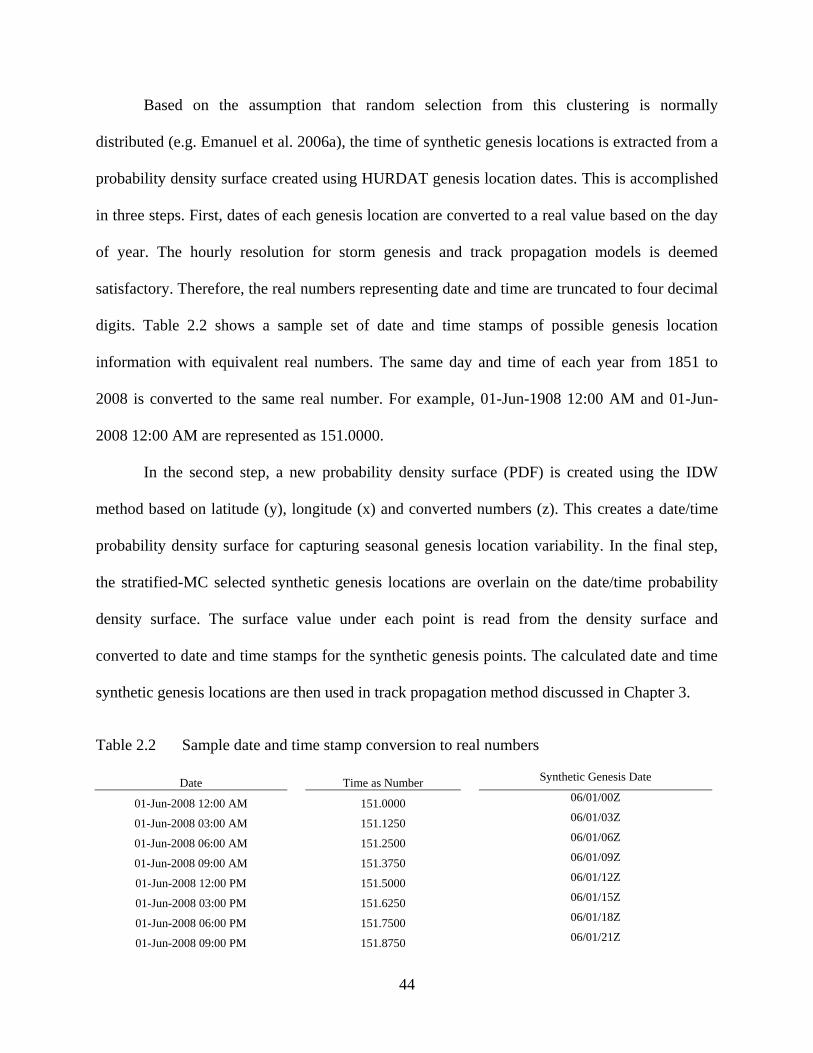
44

Based on the assumption that random selection from this clustering is normally

distributed (e.g. Emanuel et al. 2006a), the time of synthetic genesis locations is extracted from a

probability density surface created using HURDAT genesis location dates. This is accomplished

in three steps. First, dates of each genesis location are converted to a real value based on the day

of year. The hourly resolution for storm genesis and track propagation models is deemed

satisfactory. Therefore, the real numbers representing date and time are truncated to four decimal

digits. Table 2.2 shows a sample set of date and time stamps of possible genesis location

information with equivalent real numbers. The same day and time of each year from 1851 to

2008 is converted to the same real number. For example, 01-Jun-1908 12:00 AM and 01-Jun-

2008 12:00 AM are represented as 151.0000.

In the second step, a new probability density surface (PDF) is created using the IDW

method based on latitude (y), longitude (x) and converted numbers (z). This creates a date/time

probability density surface for capturing seasonal genesis location variability. In the final step,

the stratified-MC selected synthetic genesis locations are overlain on the date/time probability

density surface. The surface value under each point is read from the density surface and

converted to date and time stamps for the synthetic genesis points. The calculated date and time

synthetic genesis locations are then used in track propagation method discussed in Chapter 3.

Table 2.2 Sample date and time stamp conversion to real numbers

Date

Time as Number

Synthetic Genesis Date

01-Jun-2008 12:00 AM

151.0000

06/01/00Z

01-Jun-2008 03:00 AM

151.1250

06/01/03Z

01-Jun-2008 06:00 AM

151.2500

06/01/06Z

01-Jun-2008 09:00 AM

151.3750

06/01/09Z

01-Jun-2008 12:00 PM

151.5000

06/01/12Z

01-Jun-2008 03:00 PM

151.6250

06/01/15Z

01-Jun-2008 06:00 PM

151.7500

06/01/18Z

01-Jun-2008 09:00 PM

151.8750

06/01/21Z

45

2.8 Data Analysis and Results

The data analysis process consists of quality assessment of the historical genesis locations

and comparison of genesis creation results (synthetic against synthetic datasets, and synthetic

against historical datasets). The quality of historical genesis location data is evaluated using

spatial t-test analysis and spatial exceedance probability. In addition, the synthetic genesis

locations are compared against other synthetic sets (e.g. set A vs. set B) and historical data. The

data comparisons are used to assess the similarity and differences of the historical and synthetic

genesis locations. In the following sections, the data analysis methodology and results are given.

Historical Genesis Location Quality 2.8.1

This section focuses on exploratory data analysis for evaluation of statistical differences

within the HURDAT historical dataset. To assess the similarity and differences for various time

periods and to investigate the influence of the Atlantic Multi-decadal Oscillation (AMO) on the

historical genesis locations, spatial two-sample t-tests and spatial exceedance probability

analyses will be performed on the historical HURDAT genesis data. The purpose of this analysis

is to assess the suitability of the HURDAT dataset periods for use in the synthetic genesis

location sampling process (Stage 2).

The AMO refers to long-term changes between cool and warm phases of sea surface

temperature in the North Atlantic Ocean. These changes eventually influence tropical cyclone

activity, which creates variability in genesis locations. The annual variability of storm genesis

locations in the North Atlantic Basin has been attributed to a number of factors, such as sea

surface temperature (SST) (Elsner and Kara 1999, Batty et al. 2005), waves (Haggard 1958) and

atmospheric disturbances (Elsner and Kara 1999, Emanuel 2005a). Figure 2.15 shows the

monthly average AMO departure values above and below the mean (orange and blue bars) and

the 12-month moving average (thick black line) for the AMO between 1856 and 2008 in °C,

46

where negative values indicate periods of lower hurricane activity and higher values indicate

increased hurricane activity. For example, during the warm AMO period from 1998 to 2008,

there were on average 15 storms per year, whereas during the cool AMO period from 1970 to

1980, there were only on average 10 tropical storms per year . The period 1945-2010 contains

almost a full high and low activity cycle (i.e. two half cycles of high activity, and one full cycle

of low activity).

Figure 2.15 A) Monthly values for the Atlantic Multi-Decadal Oscillation index from 1856 to

2008, b) tropical storm count by year (After Rosentod 2010)

47

The periods for evaluation are chosen based on technological milestones and AMO

fluctuations. Based on technological milestones, the years 1900, 1945, and 1970 are key dates

because of significant advances in observational technologies. The oscillation changes (i.e. from

low to high and high to low) in AMO activity occur at approximately 1900, 1930, 1965, and

1995. Therefore, the years 1945 and 1970 are identified as the most important dates for changes

in both observational data quality for the North Atlantic Basin and in the AMO. The 1970-2010

includes roughly a partial low AMO cycle (1970-1994) and a partial high AMO cycle (1995-

2010). Additionally, the observational technology during this period is the best available.

Therefore, the historical genesis data from 1970-2010 is assumed to be the most accurate and

complete, compared to earlier time periods with observation technologies that provided less than

comprehensive coverage of the North Atlantic Basin. The following analyses investigate if

genesis data from other periods have statistically similar spatial distributions for use in creating

the probability density surface for the proposed methodology. Spatial T-Test Analysis

In this section, the two-sample t-test is selected for the purpose of spatial distribution

evaluation. The zonal t-test results (i.e. Spatial T-Test) assess the similarities and differences of

the spatial distributions of genesis locations. It is performed to investigate the possibility of

extending the time interval of genesis locations for computing the probability density surface

from 1970-2010, which is considered to be of highest quality, to 1945-2010, which would

provide more samples for probability density surface creation. The paired two-sample t-test

performs a test of hypothesis (null hypothesis) that two samples are independent random samples

from the normal distribution with equal means and equal but unknown variances. The alternative

hypothesis is that the two sample means are not equal. In this study, the data samples represent

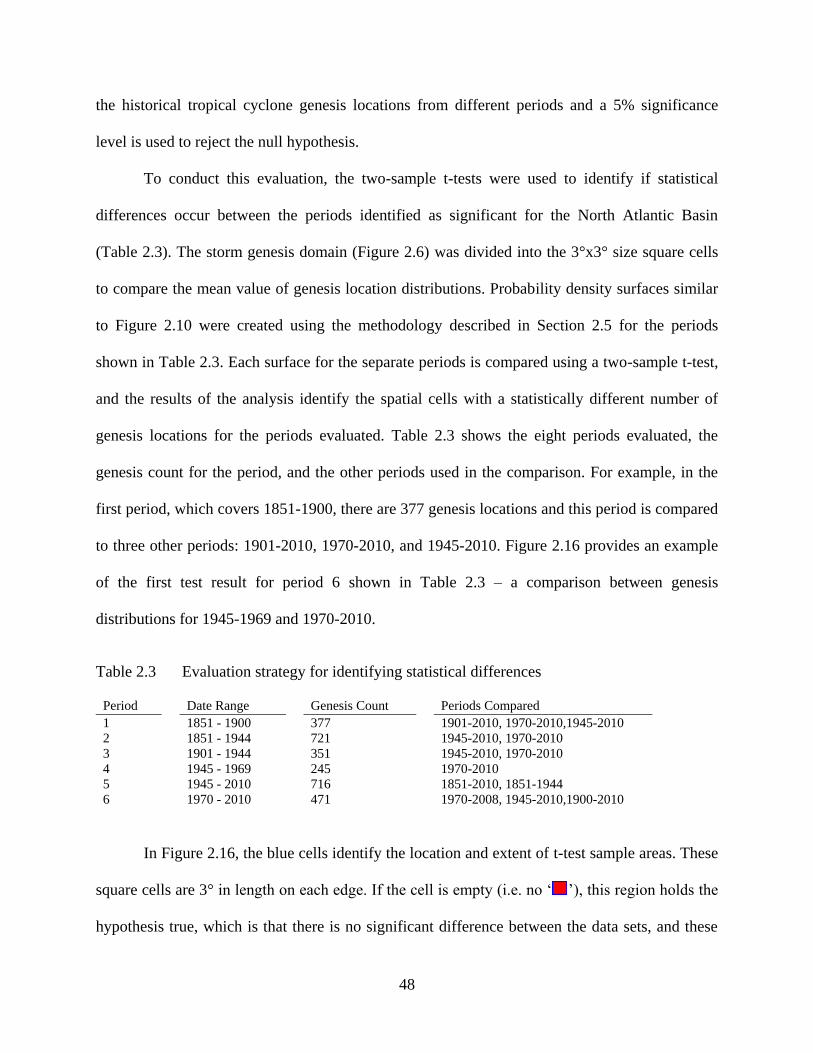
48

the historical tropical cyclone genesis locations from different periods and a 5% significance

level is used to reject the null hypothesis.

To conduct this evaluation, the two-sample t-tests were used to identify if statistical

differences occur between the periods identified as significant for the North Atlantic Basin

(Table 2.3). The storm genesis domain (Figure 2.6) was divided into the 3°x3° size square cells

to compare the mean value of genesis location distributions. Probability density surfaces similar

to Figure 2.10 were created using the methodology described in Section 2.5 for the periods

shown in Table 2.3. Each surface for the separate periods is compared using a two-sample t-test,

and the results of the analysis identify the spatial cells with a statistically different number of

genesis locations for the periods evaluated. Table 2.3 shows the eight periods evaluated, the

genesis count for the period, and the other periods used in the comparison. For example, in the

first period, which covers 1851-1900, there are 377 genesis locations and this period is compared

to three other periods: 1901-2010, 1970-2010, and 1945-2010. Figure 2.16 provides an example

of the first test result for period 6 shown in Table 2.3 – a comparison between genesis

distributions for 1945-1969 and 1970-2010.

Table 2.3 Evaluation strategy for identifying statistical differences

Period Date Range Genesis Count Periods Compared

1 1851 - 1900 377 1901-2010, 1970-2010,1945-2010

2 1851 - 1944 721 1945-2010, 1970-2010

3 1901 - 1944 351 1945-2010, 1970-2010

4 1945 - 1969 245 1970-2010

5 1945 - 2010 716 1851-2010, 1851-1944

6 1970 - 2010 471 1970-2008, 1945-2010,1900-2010

In Figure 2.16, the blue cells identify the location and extent of t-test sample areas. These

square cells are 3° in length on each edge. If the cell is empty (i.e. no ‘ ’), this region holds the

hypothesis true, which is that there is no significant difference between the data sets, and these

49

cells are considered to “pass”. If there is a red colored ‘ ’ in the cell, the hypothesis failed,

indicating a significant difference between the datasets, and these cells are considered to “fail”.

The failed regions on the edges of the computation domain may have non-data (null) density

surface values inside the cells, such as cells over the islands and land. Therefore, these cells are

excluded from the comparison of the two data sets and are considered “non-compute” cells.

Figure 2.16 A) Hypothesis test results for periods 1945 to 1969 and 1970 to 2010, B) Red dots

indicates that mean of 1970 to 2010 is smaller than mean of 1945 to 1969 (opposite

is valid for blue dots).

50

Table 2.4 The determination of pass, fail and non-compute blocks with the hypothesis testing

for considered periods

Test Years/

Periods

1851 to 1900

1901 to 1944

1945 to 1969

1901 to 1944

Pass: 250

Fail: 22 (5.6%)

Non-compute: 118

1945 to 1969

Pass: 253

Fail: 11 (2.8%)

Non-compute: 126

Pass: 250

Fail: 7 (1.8%)

Non-compute: 133

1970 to 2010

Pass: 274

Fail: 22 (5.6%)

Non-compute: 94

Pass: 273

Fail: 21 (5.4%)

Non-compute: 96

Pass: 279

Fail: 11 (2.8%)

Non-compute: 100

The percentage of fails changes from 2.3% to 5.6% for the periods listed in Table 2.4.

This indicates that the dissimilarities between the periods are negligible with respect to the

number of genesis occurrences. Also, if all genesis location are considered as a whole (i.e. the

total number of genesis events for the period), there is no difference between the periods (p value

is 1). The results for these analyses indicate that there is no significant difference between any of

the evaluated datasets. In another words, the two sample t-test does not distinguish any

difference in probability of genesis occurrence for each period investigated.

Based on t-test, the number of genesis occurrences in each of the computational cells is

similar for the periods evaluated. However, the similarity of genesis locations for different

periods is not necessarily adequately assessed because the cell size used in the test (3 x 3

degrees) is quite large. Using a smaller cell size to perform this analysis would not be

meaningful because of the to 2.5 degree kernel size. Therefore, another approach is needed to

test the similarity of the genesis locations for the identified periods. To identify the similarity and

dissimilarity of the genesis locations, the density surface of exceedance probability differences

are compared.

51

2.8.1.2 Spatial Exceedance Probability Analysis

The exceedance probability refers to the probability of an event being greater than or

equal to a given specified value. In our case, the event represents the latitude and longitude of a

genesis location. In this section, the goal is to investigate the exceedance probability of the

spatial density distribution of historical genesis locations for different periods in order to assess

the similarities and dissimilarities between these periods. Figure 2.17 provides the exceedance-

probability differences of the HURDAT dataset genesis locations for 1851-2010 and 1945-2010.

Areas within one standard deviation of the mean are shaded a light green color and are assumed

to have statistically similar distributions of genesis points. Areas greater than one standard

deviation below the mean (i.e. red-colored areas) represent the spatial extents where genesis

locations were statistically lower in the period 1851-1944 than in 1945-2010. Areas greater than

one standard deviation above the mean (i.e. blue-colored areas) represent the spatial extents

where genesis locations were statistically higher in the period 1851-1944 than in 1945-2010.

This spatial distribution of the results was expected because of the lack of observational

technology that existed prior to 1945. The red-colored areas indicate locations where hurricane

geneses likely occurred but were unreported because of the reliance on ship reports to document

tropical cyclones over water. Therefore, these storms were likely not identified until they were

nearer to the northern coast of South America and in the Caribbean Islands, an area that shows

over reporting of hurricane geneses, indicated with blue shading. In this analysis, some

significant spatial differences are observed. This finding was expected due to data quality

problems such as the absence and inaccuracy of genesis location observations, especially away

from land, for large spatial extents. The results of the exceedance probability comparison support

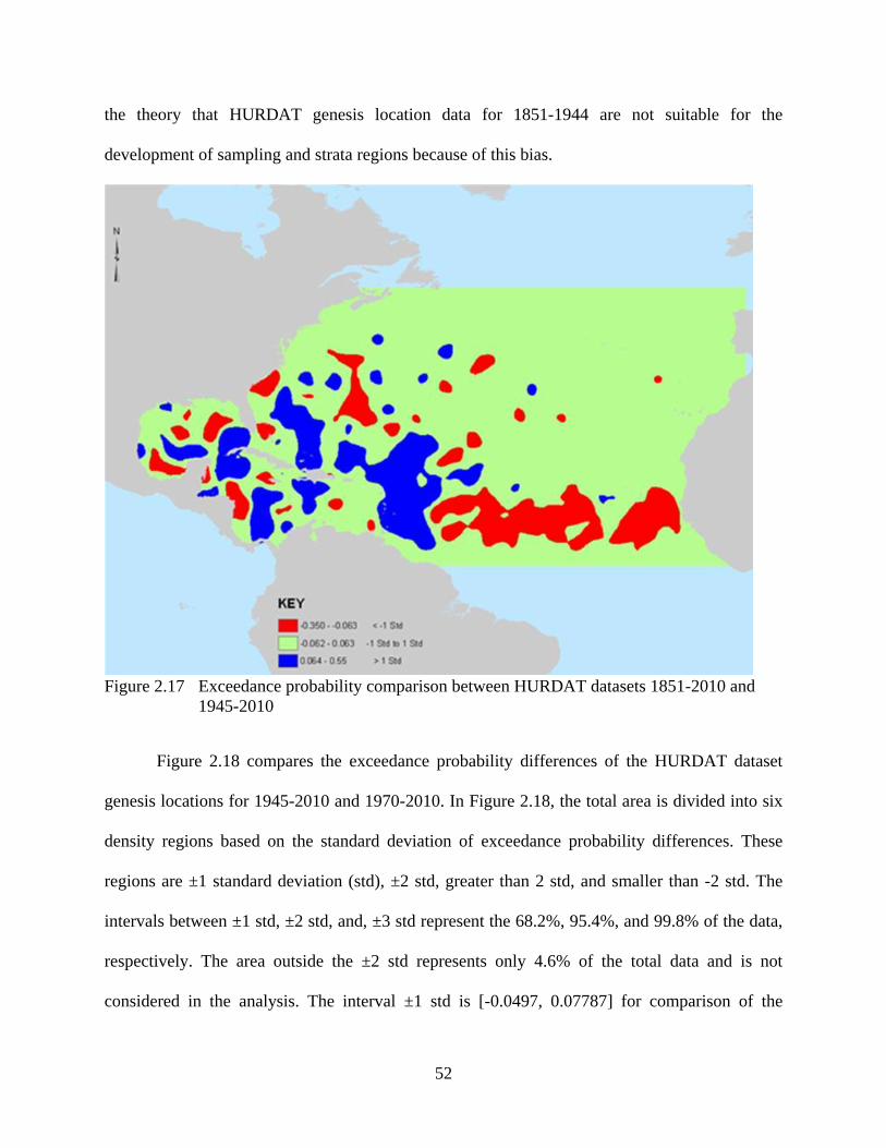
52

the theory that HURDAT genesis location data for 1851-1944 are not suitable for the

development of sampling and strata regions because of this bias.


1945-2010

Figure 2.18 compares the exceedance probability differences of the HURDAT dataset

genesis locations for 1945-2010 and 1970-2010. In Figure 2.18, the total area is divided into six

density regions based on the standard deviation of exceedance probability differences. These

regions are ±1 standard deviation (std), ±2 std, greater than 2 std, and smaller than -2 std. The

intervals between ±1 std, ±2 std, and, ±3 std represent the 68.2%, 95.4%, and 99.8% of the data,

respectively. The area outside the ±2 std represents only 4.6% of the total data and is not

considered in the analysis. The interval ±1 std is [-0.0497, 0.07787] for comparison of the

53

periods 1945-2010 and 1970-2010. The mean and the standard deviation of the exceedance

probability differences are 0.0088 and 0.055, respectively. These values are closer to zero than

the values for the period of 1851-1944 and 1945 -2010 (mean: -0.0259, standard deviation:

0.108).


1970-2010

As the mean approaches the zero, the differences between the periods diminish. Since the

mean of the exceedance probability difference, 0.0088, is closer to zero, and its standard

deviation is smaller, 0.055, the period of 1945 to 2010 is more reliable for use in synthetic

genesis location simulations than the period of 1851 to 2010. The two-sample t-test results do not

counter the findings from the exceedance probability difference approach, that there is no

54

significant difference in hurricane genesis locations for the periods 1945-1969 and 1970-2010.

This result was anticipated because of the better sampling population after 1945 resulting from

increases in observational technology. Additionally, each period contains low and high AMO

activity cycles, so effects of the AMO on the spatial distribution of genesis locations are

minimized. Therefore, it is concluded that the HURDAT genesis locations from period of 1945-

2010 are suitable for the development of the sampling/strata regions used in Phase 2 of the

genesis methodology.

Figure 2.19 Comparisons of two synthetic genesis points using the probability density surface

created using HURDAT data from 1970 to 2008.

Comparison of Synthetic Genesis Locations 2.8.2

Using the approach described in Section 2.6 of this chapter, a number of sets of synthetic

hurricane genesis points were created using the probability density surface developed with the

cleaned HURDAT genesis location data from 1945 to 2010. Because the datasets are

55

probabilistically generated, the genesis locations will be in different absolute locations for each

simulation run, but the spatial distribution of the points is statistically similar. Two sets of

synthetic genesis points are mapped in Figure 2.19 to visualize the spatial distribution of

synthetic genesis points in the North Atlantic Basin and to demonstrate both the similarity and

variation that exists between synthetic datasets. The exceedance probability is determined to

evaluate the spatial distribution of synthetic data sets. The exceedance probability charts (Figures

20 and 21) show very high correlation between the data sets south of 30°N and east of 90°W,

confirming that although there are differences in absolute location between the two synthetic

datasets, they are statistically similar in their spatial distribution in the Gulf of Mexico study

region.

Figure 2.20 Latitude exceedance probability chart for two synthetic genesis location datasets

1970-2008

56

Figure 2.21 Longitude exceedance probability chart for two synthetic genesis location datasets

1970-2008

Figure 2.22 Comparisons of HURDAT dataset (1970-2008) and synthetic genesis locations

created from 1970 to 2008 (Set 1 in Figure 2.19) HURDAT probability density

surface

57

Figure 2.23 Latitude exceedance probability chart for synthetic and HURDAT genesis location

datasets from 1970 to 2008

Figure 2.24 Longitude exceedance probability chart for synthetic and HURDAT genesis

location datasets from 1970 to 2008

0.001

0.01

0.1

1

0 10 20 30 40 50

Ex

ceed

an

ce P

rob

ab

ilit

y

Latitude (Decimal Degrees --North)

HURDAT Latitude 1970 to 2008

Synthetic Latitude 1970 to 2008

0.001

0.01

0.1

1

0 10 20 30 40 50 60 70 80 90 100

Exce

edan

ce P

rob

ab

ilit

y

Longitude (Decimal Degrees --West)

HURDAT Longtitudes from 1970 to 2008

Synthetic Longtitudes from 1970 to 2008

58

2.9 Summary

This chapter presented a new methodology for creating synthetic tropical cyclone genesis

locations for the North Atlantic basin. Relevant existing methodologies of genesis location

estimation were investigated to identify tropical cyclone databases and statistical and non-

statistical methods for prediction of synthetic genesis locations. HURDAT historic tropical

cyclone records were utilized in development of the synthetic genesis creation methodology for

the Gulf of Mexico. Although HURDAT is the official tropical cyclone record of the National

Hurricane Center, data quality and completeness issues were identified for historic genesis

locations and are discussed in more detail in Chapter 3 and 5. Because of the required data

quality for probabilistic generation of genesis locations, only the historical tropical cyclone

records after 1945 were used in the synthetic genesis simulations for the North Atlantic Basin.

In this chapter, a new approach for generating synthetic hurricane genesis locations was

proposed by combining two stages of data exploration: 1) the process of statistical inference and

2) the process of spatial sampling. This approach provided a means to expand historical records

while preserving the spatial characteristics of genesis locations. The demonstrated statistical

inference and spatial sampling processes combine usage of stratified-Monte Carlo, IDW, and

Gaussian Kernel estimation methods for the North Atlantic Basin. In this newly developed

methodology, the coordinate, date and time information from genesis locations in the HURDAT

database are used for creating and populating synthetic hurricane locations using data from

probability density surfaces created using IDW interpolation. The distribution of synthetic

genesis locations utilized the stratified-MC method, which was selected for its advantages over

other sampling methods, including a more efficient sampling algorithm, better uniform sampling,

and improved space filling properties. The statistical analysis of synthetic genesis locations

shows a high correlation between probabilistic synthetic datasets, as well as with the HURDAT

59

historical hurricane genesis location data. The output of the synthetic genesis location

methodology will serve as the input for a probabilistic track model in Chapter 3. Chapter 3

provides a detailed explanation of the integration of the synthetic genesis methodology

developed in this chapter with the track model.

60

CHAPTER 3: STORM TRACK GENERATION


This chapter focuses on the statistical prediction of tropical cyclone tracks with a known

genesis location in the North Atlantic Basin. Within the context of the overall goal of the

dissertation, the purpose of this chapter is to investigate existing tropical cyclone track

simulation models to understand the current state of the art and to identify track simulation

model components for implementation in a synthetic track methodology for the North Atlantic

Basin as part of the proposed fast-running, geodatabase-assisted storm surge modeling

framework. The first section of this chapter provides a review of existing tropical cyclone track

simulation models and the second section outlines the proposed synthetic track prediction

approach. The third section provides an assessment of the implemented track methodology

results. The synthetic track propagation methodology will utilize the genesis locations produced

in Chapter 2 as the storm origin. Both synthetic and historical storm track data will be combined

in a geodatabase framework (Chapter 5) for seamless integration with storm surge model results

(Chapter 4).

3.2 Introduction

Historical and historically representative tropical cyclone tracks are required as inputs for

developing ensemble-based statistical estimates of storm surge. The main shortcomings of North

Atlantic Basin historical tropical cyclone records are the small number of hurricane events and

missing storm strength parameters. The HURDAT dataset contains storm information for

approximately 160 years, although many of these data are inconsistent because of poor

observational technologies. These inconsistencies result from missing or inaccurate intensity data

values and poor positional accuracy of coordinates in the historical data. This short record length

61

impedes long-term trend estimations and limits the ability to make statistical inferences for

longer periods.

The absence of storm intensity parameters in HURDAT records, specifically the radius of

maximum winds (RMW) and Holland B parameter, significantly hinder storm surge estimation

for these storms. Furthermore, there are issues in the HURDAT historical dataset related to

higher wind speed and lower central pressure values for various decades caused by the choice of

calculation practices. For example, measured hurricane wind speeds during the 1930s are higher

than those measured during the 1950s (Hagen et al. 2012, Landsea et al. 2008). To overcome

these limitations, it is necessary to utilize tropical cyclone track models to simulate and expand

historical track datasets with statistically representative synthetic tracks, while also addressing

inconsistencies in the historical dataset.

Tropical cyclone track models are generally classified into three types: non-forecast

models, forecast models, and intensity forecast models. Non-forecast models are primarily used

to understand the statistical properties and trends of tropical cyclones, but they are not used to

develop advisories for particular events. Forecast models are operational models utilized by

government meteorological forecast offices to predict the propagation of existing storms.

Intensity forecast models are sometimes integrated with forecast models and are used to predict

changes in storm intensity. Appendix C provides detailed information about track forecast

models, and intensity forecast models, and reviews several models of each type.

Of these model types, a non-forecast track model is generally most appropriate for

synthetic track simulations. For example, models developed by Vickery et al. (2000b) and

Emanuel et al. (2006b, 2006a) have been used for simulation of tropical cyclone tracks in the

North Atlantic Basin. In these studies, synthetic hurricane tracks were simulated to expand the

62

historical tropical cyclone track database to contain a sufficient number of storms to make

hurricane risk assessments. Non-forecast models (Table 3.1) implement a number of

methodologies for location estimation, including pseudo-Monte-Carlo (MC) sampling (Emanuel

et al 2006b, 2006c; Rumpf et al. 2007), regression (Vickery et al 2000b, James and Madison

2005, and Darling 1991), and random sampling (Hall 2007a and Hall and Jewson 2007b). The

primary limitations of existing non-forecast models include public unavailability (Emanuel et al.

2006b, Emanuel et al. 2006a), model sampling bias (Vickery et al. 2000c), and limited sampling

data (Hall and Jewson 2007, Vickery et al. 2000c).

Table 3.1 Storm track non-forecast models

Model Name

References Mathematical Solution Type

Darling (Darling 1991) Statistical

Emanuel A

(Emanuel et al. 2006a, Emanuel et al. 2006b) Statistical

HJ

(Hall and Jewson 2007) Statistical

JM

(James and Mason 2005) Statistical

Rumpf

(Rumpf et al. 2007) Statistical

Vickery

(Vickery et al. 2000c) Statistical

Emanuel B

(Emanuel et al. 2006a, Emanuel et al. 2006b) Statistical-Dynamical

To overcome these limitations, this chapter presents a HURRAN-like non-forecast track

methodology to expand historical datasets that is computationally fast-running, easy to use, and

publicly available. The track propagation simulations begin with reduced locational bias because

of the utilization of a stratified-Monte Carlo method for sampling of genesis locations (Chapter

2). The common weakness of positional calculations in other statistical models is eliminated

through the use of GIS geospatial libraries (Batty et al. 2005). HURRAN model computes

stronger wind speeds compared with the historical records (Neumann and Hope 1972). In order

to reduce wind speed over estimation, wind speed values are adjusted in the modified-HURRAN

model. Further, additional track intensity parameters (e.g. RMW, Holland B) are estimated for

63

tropical cyclone tracks, which are required inputs for storm surge estimation (Chapter 4). The

approach for this methodology is to simulate hurricane lifecycle stages after formation (Chapter

2) to dispersion. This chapter focuses on tropical cyclone development (track propagation) and

dispersion (track termination) stages of the lifecycle with an approach that consists of three

procedures: 1) data input based on synthetic and historical genesis data, 2) track propagation

based on historical track data, and 3) track output.

3.3 Storm Track Methodology Framework

The proposed methodology is a GIS-integrated, fast-running, statistically-based non-

forecast model that reduces shortcomings of existing models implemented for the North Atlantic

Basin. The storm track propagation process is simply an iterative estimate of synthetic storm

locations and related intensity parameters using genesis location information as an initial

simulation start point. There are a number of types of track propagation models (Appendix C);

however, many of these model types (e.g. statistical-dynamical, statistical-barotropic) require

ancillary meteorological and oceanographic data, while statistical models do not require data

outside of the parameters being modeled. Long-term historical datasets of meteorological and

oceanographic variables corresponding with the length of the historical tropical cyclone track

records do not exist. Therefore, a statistical track propagation methodology utilizing the

historical tropical cyclone record is most appropriate.

The storm track methodology is summarized in three stages (Figure 3.1): 1) synthetic

genesis location data as input, 2) track propagation as tropical cyclone simulation, and 3)

synthetic storm track as output. After the creation of genesis locations (calculated in Chapter 2),

each of the synthetic genesis point locations is used as an initial starting location for the synthetic

track propagation module. The propagation procedure is implemented as a six-step procedure to

create synthetic storm tracks:

64

1. The current segment location is initially equal to the genesis location and is updated

through each iteration.

2. The likely location of the next segment is estimated using probability density function

(PDF) results from identified storm analogs and their related parameters (e.g. latitude,

longitude, wind speed, date, time and direction).

3. Storm intensity parameters (e.g. wind speed, central pressure, RMW, and Holland B) are

calculated for the segment. These calculated intensity parameters are adjusted based on

the sub-domain and historical records.

4. Segment time and date are calculated, initially based on the genesis spatial-temporal

information, and updated through each iteration.

5. Track termination conditions are checked based on the predefined rules (e.g. wind speed)

to determine if the storm is terminated or if another propagation iteration is performed.

6. All simulated segments are smoothed using spline interpolation to reduce segment

discontinuities.

Figure 3.1 Synthetic storm track methodology framework

65

The calculated synthetic tracks and their properties are exported to a geodatabase and an

ASCII file format, which are used in storm surge estimation methodology (Chapter 4). ASCII

files can be utilizes as an input file with ADCIRC model for running storm surge simulations.

Input Datasets 3.3.1

The proposed model requires two input datasets. First, the track simulation methodology

is designed based on the assumption that the genesis locations of the simulated storms are

known. These data are generated using the synthetic genesis module presented in Chapter 2.

Second, the methodology is a statistical tropical cyclone simulation model, which requires

historical track analogs for the track propagation. The HURDAT historical track dataset

represents the official tropical cyclone track history for the North Atlantic Basin (Jarvinen and

Caso 1978) and is used to provide these historical track analogs.

The HURDAT archive is referred as the best track database for the North Atlantic basin

and contains information for 1457 storms from 1851 to 2010 (Jarvinen and Caso 1978, Landsea

et al. 2003). As an example, Figure 3.2 displays a subset of selected storms and their genesis

points from HURDAT for the period 1970-2008. Despite the fact that HURDAT is the best

available historic dataset for the North Atlantic, it is not error free. Spatial, temporal, and

intensity errors have generally resulted from primitive observation technologies (McAdie et al.

2009) and human effects (Jarvinen and Caso 1978, Jarvinen et al. 1984).

Spatial and temporal discrepancies in HURDAT are prevalent in the pre-1944 data,

caused by observation and data recording practices. At the most extreme end of these

discrepancies, Landsea et al. (2008) estimated that three to four tropical cyclones may not have

been recorded yearly in HURDAT from 1886 to 1920, which is one the order of 100 to 130

storms over this 34 year period. The practices used in recording storm locations have also

contributed to errors within the historical dataset. Prior to 1931, only the 12:00 Greenwich Mean

66

Time (GMT), or Zulu (Z) position of a storm was recorded (Jarvinen and Caso 1978). The

remaining 0:00Z, 06:00Z and 18:00Z positions were interpolated from 12:00Z positions. This

practice contributed, in part, to estimated average track position errors of approximately 100

nautical miles for this period (Jarvinen et al. 1984). In addition, the utilization of ship

observations led to further errors in track position prior to 1900, when position estimates were

reported with an accuracy of 0.5° to 1.0° latitude-longitude (Landsea et al. 2008).

Modern historical records are much more complete and have higher accuracy because of

the use of aircraft for storm reconnaissance beginning in 1944 (Hagen et al. 2012, Perina 2012)

and with the use of weather satellites in the 1960s (Elsner and Kara 1999). Today, the exact

location of a tropical cyclone is known through complete satellite observation coverage 24 hours

a day in the North Atlantic. Within the HURDAT dataset, the positional data for all records are

recorded in decimal degrees with one decimal precision (e.g. 29.1°N and 90.4°W), which makes

the spatial location information accurate to approximately 10 km in the Gulf of Mexico. Intensity

discrepancies in HURDAT result from both incomplete early historical records and less accurate

intensity parameters. Prior to 1905, the observation of tropical cyclone in the whole North

Atlantic basin was not possible due to inadequate reconnaissance technologies. This caused the

dearth in the recorded wind speed and central pressures values (McAdie et al. 2009). Second,

data recording practices for wind speed result in rounding of wind speed to the nearest 5 knot

value in records (Hope and Neumann 1971, Jarvinen and Caso 1978, Landsea et al. 2008). For

example, a 68 knot wind speed is recorded as 70 knots, while a 67 knot wind speed is recorded

as 65 knots in HURDAT. The most significant drawback of the HURDAT dataset is non-

inclusion of intensity parameters that are required for storm surge estimation, such as wind radii

and Holland B data. This incomplete and less accurate early historical records lead to decrease in

67

the reliability of track intensity estimation and consequently inaccurate storm surge estimation

from these intensity parameters.

Figure 3.2 Sample subset of HURDAT storm genesis locations and associated tracks from

1970 to 2008

There have been a number attempts to increase the reliability of HURDAT by correcting

systematic biases (e.g. Landsea et al. 2008, Landsea et al. 1999, McAdie et al. 2009). However,

it is not possible to correct some of the biases in HURDAT, such as adding unrecorded tropical

cyclones into the dataset. Therefore, issues related to unrecorded storms are ignored. For the

intensity parameter calculations, spatial-temporal issues are taken into account with

incorporation of a two-pass verification approach. During the first pass, intensity adjustment

equations are developed based on the complete historical records. During the second-pass

(simulation), the intensity adjustments are applied to synthetic tracks to minimize effects of data

errors. In addition, the adjusted values are used to calculate RMW and Holland B parameters for

utilization in storm surge estimations (Chapter 4).

68

Model Computational Environment 3.3.2

Geographic Information Systems (GIS) is an ideal platform for storage and spatial

calculations related to tropical cyclone tracks. GIS provides a computational environment for

real world objects within the geographic space by using geographic form and geographic

relationships (de Smith et al. 2007) and is increasingly becoming the primary method to capture

and handle geographic data for spatial analysis (Batty et al. 2005, Johnston 2001, Maguire et al.

2005). GIS provides a computational environment for managing tropical cyclone data (e.g.

tropical cyclone track data), computing spatial relationships (e.g. coordinates, distances,

directional relationships), and visualizing raw data and computed results (e.g. maps, probability

density surfaces) (Durr and Gatrell 2004, Johnston 2001, Mitchell 1999, Mitchell 2005,

Murayama and Thapa 2011, Zeiler 1999).

GIS is an ideal platform for handling spatial location representation (i.e. projection

transformation), spatial distribution, and relationship calculations (i.e. spatial statistics) of real

world objects because of provided spatial libraries for computations (Longley and Batty 2010,

Mitchell 2005, Murayama and Thapa 2011, Peters 2008). The benefits of implementing a GIS

computational environment for the track propagation methodology are twofold. First, GIS is an

ideal platform for storing and computing spatial location related numerical parameters with high

decimal precision for not only tropical cyclone tracks, but also storm surge elevation (Chapter 4).

Second, GIS reduces or eliminates projection errors by using both planar and spherical

computational domains as required. The non-forecast models reviewed in this chapter, utilize

either a single computational domain (e.g. Vickery et al. 2000b), or rough conversions between

the computational domains (Emanuel at al. 2006).

These distortions are important because they can affect the accuracy of calculated space

related parameters. For example, the track propagating methodology utilizes a density estimation

69

kernel for identifying candidate tropical cyclone segments, which is computed by using a 2.5° or

5° selection circle (a shape related computation). In addition, the headings of the identified

segments are calculated (a direction related computation). Shape and direction related

computations require utilization of two different coordinate systems. Calculations related to

shape, area, distance, and directions contain varying levels of errors, if the spatial calculations do

not utilize proper projections. As stated before, these kinds of errors negatively influence the

accuracy of various storm parameters, such as the distance, direction, and wind speed. Figure 3.3

illustrates the distortion of a shape (e.g. a circle) that occurs due to the projecting utilization.

In the geospatial measurement framework, the locations are modeled as the spherical (a

geographic coordinate projection) and planar (a projected coordinate system) spaces (Miller and

Wentz 2003, Maguire et al. 2005). In other words, a geographic system is used for representing

object locations on the curved surface, such as surface of the earth (Johnston 2001, Mitchell

1999, Zeiler 1999). For example, tropical cyclone locations in HURDAT are provided utilizing

latitude and longitude parameters, such as 22.1° North latitude, and 92.2° West longitude. On the

other hand, a projected coordinated system represents the locations of objects on a flattened

surface, such as a paper map (Johnston 2001, Mitchell 1999, Zeiler 1999). For example, the

locations and headings of a tropical cyclone are given in a planar coordinate system utilizing, and

origin, direction, speed, such as a storm located at 22.1° N, and 92.2°W coordinates and moving

with bearing of 270° at 6 mph.

Choosing representative coordinate systems during computations are very important for

spatial data representation because the accurate geospatial computations involve three concepts,

which are referencing the locations of object, considering computation related distortions and

transforming location coordinates for proper calculations. Converting location information from

70

a curved surface to a flat surface causes distortions, and this is true for all projections

conversions, such as tropical cyclone locations estimations. Depending on the properties of the

projection, the spatial properties of shape, area, distance, and direction are all subject to

distortion (Batty et al. 2005, Maher 2010, Murayama and Thapa 2011, Zeiler 1999). There is not

a projection system that can preserve all four spatial properties (Maguire et al. 2005, Maher

2010, Mitchell 2012, Murayama and Thapa 2011).

Figure 3.3 A) Shows shape distortion due to the projection B) Shows no shape distortion

because of utilized shape preserving projection

There are two approaches to minimize projection distortion errors with tropical cyclone

track models. In the first approach, all occurring errors are assumed to be within the acceptable

range (e.g. Hope and Neumann 1970). For example, the approximate location value of a tropical

cyclone with ±20 miles is accepted as an accurate location. The models mentioned in the Table

2.1 utilize this approach for geospatial computations. This is a problem because the

generalization may result selection of wrong analogs from the historical. In the second approach,

depending on the calculation, a proper projection type is selected. For example, calculating

distance and direction, the UTM projections is ideal. On the other hand, conformal projections

are ideal for preserving shapes (e.g. Lambert Conformal Conic Projection).

71

The second approach is an improvement over the first approach because the second

method minimizes the all kinds of projections related errors. In this study, the accuracy of the

proposed model is better than previously mentioned models because of the utilization of

appropriate projection type for shape, direction, and distance calculations. For example, Emanuel

et al. (2006a) utilize geographic projection and coordinates for direction calculations. In addition,

the projection conversion calculations are handled by optimized libraries in the GIS. This

provides further computational improvements, such as accurate and fast-running algorithms.

Model Domain 3.3.3

The focus area for the track propagation methodology is the Gulf of Mexico; however,

the full North Atlantic Basin study region (Figure 2.6) is utilized as the model domain to ensure

that the full range of genesis points are considered. Storms may originate outside the Gulf of

Mexico but then propagate into the Gulf during the storm lifecycle. These track propagations are

therefore captured by considering the full basin. Section 2.4.2 provides detailed information

about the selection of the study region.

3.4 Track Propagation Methodology

Underlying Computational Algorithm 3.4.1

A detailed review of existing non-forecast, forecast, and intensity models was completed

(Appendix C) to identify common mathematical model solutions and properties of existing

models. The first objective of this review was to identify whether direct implementation of

existing models would be suitable for the proposed geodatabase-assisted storm surge estimation

methodology. If this would not suitable for the proposed storm surge estimation methodology,

the second objective was to identify currently implemented parameters and pertinent model

features from existing models to inform the development of the synthetic track methodology.

The attributes of the desired track estimation methodology are:

72

1. The model must be suitable for long-term statistical predictions from the historic dataset.

2. There should be no usage or distribution restrictions.

3. The model performance should be comparable to the “official” statistical benchmark

model, CLIPER (Neumann 1972), utilized by National Weather Service.

4. The model should be optimized to reduce computational requirements, meeting the

overall objective of development of a computationally fast-running model.

Based on these desired attributes, the existing non-forecast, forecast, and intensity models

are removed from consideration as a candidate models for direct implementation. Existing

models are also reviewed to identify attributes for modified implementation into the model.

Statistical-synoptic, statistical-dynamical, dynamical-barotropic and dynamical-baroclinic

models require climatological information and are not suitable for a statistical implementation

and are removed from consideration (attribute 1). Next, several existing tropical cyclone models

(Emanuel et al. 2006a) are proprietary and therefore not publicly available (Ravela 2010). For

these models, there are restrictions on implementing existing methodologies, and distributing

results of these models, especially for the non-forecast models. Models with proprietary

components are therefore also eliminated from consideration (attribute 2). Because of the model

performance related to be comparable to the “official” benchmark model, models by Vickery et

al (2000b), Darling (1991), Hall and Jewson (2007b), James and Madison (2005), and Rumpf

(2007) are also are eliminated from the candidate list. Remaining HURRAN and CLIPER

models are compared based on the computational complexity. CLIPER model is filtered out

because the last model criteria since HURRAN is a faster-running model than CLIPER.

Based on the model attribute criteria, an existing model was not found for direct

implementation. However, the HURRAN model (see Appendix D; Hope and Neumann 1970)

73

was identified as the model that met the greatest number of desired attributes, although several

modifications and updates are needed for implementation in the geodatabase storm surge

methodology. HURRAN was one of the earliest forecast models developed (Appendix C) and is

entirely statistical (i.e. dynamical integration of climatological factors are not considered). This

statistical tropical cyclone track model is available without use restrictions. Finally, this model

outperforms CLIPER’s locational accuracy in the Gulf of Mexico (Neumann and Hope 1972).

Finally, the model algorithm is a fast-running algorithm compared with other existing models.

As a forecast model, HURRAN was used to statistically predict the propagation of a tropical

cyclone based on historical analogs, but failed to capture effects of climatological conditions and

therefore did not perform well for recurving storms (Heming and Goerss 2010, Neumann 1972,

Neumann and Hope 1972). HURRAN was replaced as a forecast model by CLIPER, which is

used as the benchmark for forecast models today (Neumann and Pelissier 1981).

In spite of the advantages of HURRAN, there are two well-known disadvantages

(Neumann and Hope 1972): 1) track location errors for latitudes above 30°N, and 2) over

estimation of wind speeds at landfall. Because the goal of this research is to develop a model for

the Gulf of Mexico, the first disadvantage is not considered. For storm surge modeling in

general, overprediction of wind speeds in forecast models is preferred to underprediction of wind

speeds because the slightly higher wind speed compensates for the exclusion of waves from

storm surge model computations (e.g. ADCIRC) (Forbes et al. 2010). In terms of the storm surge

estimation methodology developed in Chapter 4 and non-forecast models, however, this is

undesirable. Therefore, the second well-known disadvantage of the HURRAN model, wind

speed overestimation, is addressed in the proposed methodology.

74

Additionally, several other modifications to the HURRAN model are made to increase

performance, update the computational environment, and estimate storm parameters needed for

storm surge modeling (Table 3.2). The original HURRAN model and the proposed model are

products of different programing paradigms and structures because of the implemented

computational environments. For example, the proposed methodology is designed based on

object-oriented programming, using a collection of objects and classes in GIS. These

modifications improve intensity parameter (e.g. wind speeds) calculations, spatial (e.g. segment

selection) calculations, and I/O (e.g. data storage) operations. All these improvements contribute

to the development of a fast-running methodology. These modifications are summarized in Table

3.2.

Table 3.2 Comparison of original HURRAN implementation and proposed model to highlight

improvements

Component

HURRAN Model

Proposed Model

Advantage/Improvement

Programming Paradigm Procedural Programming

Object Oriented

Improved modularity, information hiding, code

reuse, and debugging

Program Structure Made up of modules and

procedures

Collection of objects and classes

Better data encapsulation

Computational

Environment

Standalone

GIS

Improved spatial calculations and accuracy,

efficient representation of relationships between

storm parameters (e.g. storm track and surge)

Wind Speed Estimation Analogs without correction

Analogs with correction

Reduction in wind speed

overestimation/underestimation

Intensity Parameters Wind speed, central pressure

Wind speed, central pressure

RMW, Holland B

Additional intensity parameters required for storm

surge estimation

Track Termination Based on wind speed

reduction rules

Based on wind speed reduction

rules and predefined zones for

the Gulf of Mexico

More realistic track termination

Spatial Calculations Segment estimation kernel

with spatial estimation errors

Segment estimation kernel with

accurate spatial calculations

Increased accuracy and precision in calculations,

proper projection use

I/O Utilize flat file for all storms

Utilize geodatabase for all

storms, ASCII files for

individual storm for surge

models

Improved data interaction and functionality

because of geodatabase. Elimination of legacy in

I/O operations

Data Storage Flat file

Geodatabase

Improvements in data management in the

geodatabase because of DBMS.

Integration into one data container of genesis,

track and surge data

User Interaction Manual input interruptions

Automated

Automated model simulation from start to end.

The flowchart of processes for the implemented methodology for the creating synthetic

tropical cyclone tracks is given in Figure 3.4, and can be compared with the original HURRAN

75

process (Appendix D). The track propagation process (outlined with grey-dashed box) begins

after reading the genesis location data (Chapter 2) and ends with segment smoothing prior to

outputting of the synthetic track. Details about the primary stages of the track propagation

methodology are given in the following sections.

Figure 3.4 Flow chart of implemented track propagation methodology

76

Current Segment Selection 3.4.2

The “current segment location” is the starting point for each propagating track segment.

At the beginning of the simulation, the current segment location is set to the input synthetic

genesis location and the propagation methodology is implemented. Near the end of each

iteration, the current segment location is set to the endpoint of the propagated segment. The

current location selection step continues to utilize location information obtained from the

previous iteration until the track termination criteria are reached.

Estimation of Next Segment Location 3.4.3

The storm location variables used in the propagation methodology are storm direction

(heading), forward speed, date and time, radius of search circle, and date interval ranges. Among

these, storm direction, forward speed, and date and time are estimated from identified HURDAT

track segments. Default values and conditions are used for the search circle radius and date

interval ranges (Table 3.3). The values of the computed storm variables are determined from

selected subset of tropical cyclone analogs (track segment) that are identified by the combination

of the spatial and attribute queries performed in the geodatabase. The search window coverage is

a 2.5° radius circle centered at the current latitude and longitude. All historical storm segments

falling within this circle are selected from the historical track database using a spatial search

function. These selected segments are refined based on the storm date. If the date of the historical

segment differs by more than ±15 days, the segment is removed from the selection set. The

reason for this is the identification of temporally similar tropical cyclone tracks within the

moving spatial search window (search circle) (Emanuel et al. 2006a, Hope and Neumann 1970).

After that, the heading of each segment is calculated. The selection set of segments is further

refined using storm heading window criteria (Table 3.3). Figure 3.5 illustrates this process step

by step. The candidate storm segment from the selected HURDAT analogs is calculated by

77

utilizing probability density estimation kernel of the HURRAN model (Hope and Neumann

1970). The future location of the synthetic track is forecasted into 1 hour by using determined

storm forward speed and heading from the candidate track segment.

Table 3.3 Segment selection criteria

Parameter Criteria

Radius of search 2 ½ degrees

5 degrees (if there is less than 5 analog/segments in the selection)

Storm dates Current date ± 15 Days

Storm heading window 22 ½ degrees on either side of previous segment’ heading

Figure 3.5 Illustration of spatial and attribute query selections from historical analogs during

the segment calculations. A) Current location and 2.5° search radius, B) Selection

of all historical storms (analogs) that intersect the search circle, C) Filtered analogs

using ±15 day temporal window, D) Filtered analogs using heading windows

(selected analogs are shown in yellow)

78

Track Intensity Parameters 3.4.4

After identification of the next segment location, storm intensity parameters are

calculated based on the intensity of the selected candidate segment for the each 1-hour forecasted

synthetic track segments (Table 3.4). The wind speed (in knots) of the segment is computed

utilizing track propagation algorithm rules. The central pressure, RMW and Holland B

parameters are calculated with respect to storm coordinates and wind speed. Inclusion of the

intensity module in the track propagation procedure leads to smooth changes in the calculated

parameters, enhancing the stability of the calculated parameters. Calculated RMW and Holland

B parameters are not used in storm track propagation. However, these two parameters are highly

correlated with storm surge elevation. Therefore, these parameters are added as track intensity

parameters into the tropical cyclone track datasets so that they can be used in the storm surge

estimation methodology. Section 3.4.4.3 gives detailed explanation about what these parameters

are and how they are calculated.

Table 3.4 Track intensity parameters

Parameter Criteria

Wind speed If the speed of existing storm is less than 10 knot, use speed of existing storm

±5 knot.

If the speed of existing storm is from 10 through 20 knot, use 50 to 150% of

existing storm speed.

If the speed of existing storm is greater than 20 knot, use speed of existing

storm ±10 knot.

Radius of Maximum

Winds (RMW)

Computed from the Equation 3.10

Holland B Computed from the Equation 3.11

3.4.4.2 Wind Speed and Central Pressure

The initial wind speed of the first candidate segment is obtained from the information of

selected synthetic genesis location for the track propagation. The default value for the initial

79

wind speed of every genesis location is 10 knots in the domain because this wind speed value is

the threshold for the initiation and termination of a storm track. Next, a candidate segment from

HURDAT analogs is identified by using the segment estimation kernel. The wind speed of the

candidate segment is utilized for computing the wind speed of 1-hour future projected segment

based on the criteria given in Table 3.4. For example, the 1-hour future projected segment’s wind

speed is increased by 5 knot, if the speed of the candidate segment is not higher than 10 knots.

The relationship between maximum sustained surface wind speeds and corresponding

central pressure was originally developed through regression analysis of a limited number of

observations for the Atlantic Basin (Kraft 1961). Landsea et al. (2003) implemented a similar

approach using more precisely observed, and increased sample size because of availability more

records resulting improved observational technologies. The regression demonstrated a

dependency on latitude and the derived equations are used to calculate central pressure (Po, mb)

based on wind speed (Wind, knots) and North Atlantic Basin sub-region (Equations 3.6 through

3.9). Note that ambient atmospheric pressure is 1013 mb.

For GMEX ( ) (

)

Sample size =664; r=0.991 (3.1)

For < 25°N ( ) (

)

Sample size =1033; r=0.994 (3.2)

For 25-35°N ( ) (

)

Sample size =922; r=0.996 (3.3)

For 35-45°N ( ) (

)

Sample size =492; r=0.974 (3.4)

The historical HURDAT tropical cyclone dataset includes many records with missing

central pressure and wind speed values. Also, some records falling outside of the Gulf of Mexico

are not considered. These two kinds of records are eliminated from the data sets before the

regression analysis. The remaining number of records is 1617 (out of 5528). In order to decrease

over/under estimation of wind speeds in the simulated tropical cyclone tracks within the Gulf of

80

Mexico, the wind speed adjustment should be done as a function of central pressure differences

( ). Central pressure differences are computed from ambient atmospheric pressure (1013 mb)

by subtracting computed central pressures (PR) for track segments.

The correction procedure consists of two stages: 1) identification of wind speed and

central pressure difference data trend of historical and initially simulated synthetic tracks and 2)

calculation of wind speed adjustment values for synthetic tracks in the Gulf of Mexico. For the

trend identification stage, initially, a set of simulations are conducted for creating the synthetic

tropical cyclone tracks from the HURDAT data set for the analysis. Curve fittings are applied

both the historical and synthetic data sets to identify the relationship between maximum wind

speed and storm central pressure, where pressure is described as the difference between ambient

central pressure (1013 mb) and the minimum cyclone central pressure at the time the wind speed

was measured, P. Figure 3.6 shows scatter plot of the wind speed and central pressure

difference values for both historical (red ‘+’) and synthetic (blue ‘○’) data. The solid lines show

the best fit computed curve fits (Equations 3.1 and 3.2 for historic and synthetic data,

respectively) with respected colors in the Figure 3.6. The coefficient of determination (R2) values

are 0.8836 and 0.9853 for historic and synthetic datasets, respectively.

(3.5)

(3.6)

where

= 1013 – Central Pressure (PR) (mb)

Wind = Wind Speed (knots)

Wind speed adjustment values (Vratio= Vsynthetic / Vhistoric) are calculated at sampled central

pressure differences by using curve fitting equations (3.5 and 3.6). Figure 3.7 gives the change of

81

calculated wind speed ratios with central pressure differences. In this figure, three trend regions

are observed. Therefore, three curve fittings are applied at central pressure difference values of 1

- 13.89 mb, 13.89 - 38.62 mb and 38.62 - 46 mb intervals. Red lines give curve fits for these

three regions (Equations 3.7 through 3.9) and Table 3.4 summarizes fit statistics for the same

regions. With these derived relations, synthetic data should be adjusted.

Figure 3.6 Curve fit of historical and synthetic data sets

The relationships between the synthetic and historical wind speeds are derived with

regression analysis based on three central pressure difference intervals for the Gulf of Mexico

(GMEX). With these developed regression equations, the over and under estimations of synthetic

wind speeds are minimized. These improved calculations are incorporated into the modified

track propagation model.

if 13.89 mb (3.7)

if 38.62 mb (3.8)

if 38.62 mb (3.9)

82

where

= 1013 – Central Pressure (PR)

Figure 3.7 Curve fittings of wind ratios

Table 3.5 Wind speed ratio fit statistics

Parameter

Part 1

(Blue Dots)

Part 2

(Green Dots)

Part 3

(Red Dots)

SSE 2.79E-04 8.26E-05 9.37E-05

R2 0.9993 0.999 0.9983

df 13 26 54

R2 adj 0.9992 0.9989 0.9982

RMSE 0.0046 0.0018 0.0013

This table shows the goodness of the fits. All R2 values close to one. There are negligible

differences between the adjusted R2 and R

2 values. This indicates that the number of data points

are sufficient for a curve fitting. Finally, all root mean square errors (RMSE) are less than 0.05.

This show the fits are acceptable for wind speed ratio predictions from central pressure

differences.

83

Consequently, the wind speed (WIND) values are recomputed using updated central

pressure values. With these regression equations, the HURRAN model over estimation errors are

eliminated.

3.4.4.3 Radius of Maximum Winds (RMW) and Holland B Parameters

To enhance the output of the track propagation model, RMW (Rmax) and Holland B

parameters are added to each segment of the synthetic track. Specially, the RWM data is used for

creating wind fields for computing storm surge elevation in the deterministic ocean circulation

models, such as ADCIRC. These parameters are used in storm surge elevation estimation

(Chapter 4). Updated Radius of Maximum Winds (RMW or Rmax) is calculated using Equation

3.10 (Vickery et al. 2000b).

( ) ( ) (3.10)

where

RMW = distance from storm center to location of maximum winds (eyewall) (km)

= central pressure (mb)

= latitude (decimal degree)

The Holland B parameter is a shape related factor that specifies the pressure profile of a

hurricane. Furthermore, this parameter provides good correlation between pressure change,

RWM and the latitude of storm center. This parameter is proposed by Holland (1980). The

computed Holland B parameter value range changes depending on the region (e.g. 0.8 to 2.5 for

the Gulf of Mexico). In this study, the Holland B regression equation (Equation 3.11) the for

Gulf of Mexico (Powell et al. 2005) was derived updated equation by using a larger H*wind data

set recorded during aircraft reconnaissance flights. This equation is selected because of

correlation results for the model domain and HURDAT records (Vickery and Wadhera 2008).

84

(3.11)

where

B = a parameter that specifies the shape of the pressure profile (dimensionless)

RMW = distance from storm center to location of maximum winds (eyewall) (km)

= latitude (decimal degree)

= a random term chosen from a standard normal distribution

Time and Date Calculation 3.4.5

The time of each storm segment has merged into six-hour increments from the track's

genesis point time. For example, consider a synthetic storm number 1 that starts from the genesis

point 1 with a time stamp of 00:00 Zulu time, and exists for 24 hours before it dissipates. This

means that the synthetic storm will have four segments. The time stamp of first segment is 00:00

hour and the time stamp of the following segments are 06:00, 12:00, and 18:00 hours. The storm

date is computed in a similar way. As mentioned before, the initial data of the storm will be

obtained from the genesis location date. The track date will be incremented accordingly.

Track Termination 3.4.6

The process of the track segments propagation is repeated until the track termination

criteria are met (Table 3.5). After each iteration of the storm track segment creation, the storm

parameters are computed for each segment by using probability kernel and the termination

conditions are checked. Two conditions lead to start of the terminations process. These two

conditions are: 1) the storm track reaches the track creation domain boundary (as shown in

Figure 2.5) such as landfall, or 2) the number of suitable selected segments are less than five. In

either case, the storm is weakened based on the track speed rules of Segment Selection Criteria

given in Table 3.2. For example, when a storm lands on an island, the storm can continue across

85

with some reduction in wind speed. If the segment wind speed is less than 10 Knots (tropical

storm speed threshold), the storm track is terminated. Otherwise, the synthetic storm is extended

to next segment. For the second condition, there must be at least five selected analogs from the

HURDAT data set. If five satisfactory analogs from HURDAT are not available in the 2.5°

selection area, the ellipse is enlarged to a 5° radius. If there are not five satisfactory analogs in

the enlarged 5° selection area, the synthetic storm track is terminated.

Table 3.6 Track termination criteria

Criteria Value

Landfall Start wind speed reduction based on the speed rules in the Table 3.2

Minimum Wind Speed Less than 10 Knots

Minimum Segment Count 5

Radius of search 2 ½ degrees

5 degrees (if there is less than 5 segments in the selection)

Smooth Segments 3.4.7

The implemented track propagation procedure creates sub-segments of 1- hour positions

of the simulated storm. While the track propagation iterates through each sub-segment, the track

termination module is called to check track termination conditions. When the track termination is

reached, selected hourly sub-segment candidates are smoothed with the spline interpolation

(Franke, 1982) to prevent an unrealistic jagged storm path. Then, the hourly sub-segments are

merged to create 6-hour track segments. This process is repeated until the termination of the

synthetic storm.

Intermediate Track Parameters 3.4.8

Table 3.6 illustrates the intermediate data records for each one of the segments during the

calculation process. This table shows the finalized values after the completion of smooth

segments for a synthetic storm. The each row of Table 3.6 includes information regarding to

86

fifteen parameters of a segment, which are calculated during the track simulation methodology.

All parameter definitions are given at the end of the table.

Table 3.7 The intermediate track segment calculation sample records

ADV LAT LONG TIMEY TIMEM TIMED TIMEH TIMEZ WIND PR STYPE STORMID MyFID B RMW

49 36.55 -73.75337 2009 8 21 6 Z 70 981 CAT1 Storm9 304 1.3365 66.830829

50 38.305 -71.31618 2009 8 21 12 Z 70 982 CAT1 Storm9 305 1.31858 72.712942

50 39.662 -72.48676 2009 10 7 12 Z 75 979 CAT1 Storm12 431 1.30618 76.949865

33 36.673 -71.17731 2009 8 24 18 Z 75 978 CAT1 Storm14 502 1.33363 66.585324

34 38.591 -69.97479 2009 8 25 0 Z 65 985 CAT1 Storm14 503 1.31441 74.311351

14 37.296 -73.76783 2009 10 3 12 Z 55 991 TS Storm15 523 1.32565 70.892873

15 38.964 -71.82728 2009 10 3 18 Z 50 994 TS Storm15 524 1.30953 77.143128

ADV = rank of a storm segment TIMEH = hour of a storm segment STORMID = unique storm identifier

LAT = latitude of the storm eye TIMEZ = time based on ZULU MYID = unique segment identifier

LON = longitude of the storm eye WIND = wind speed in knots B = Holland B parameter (dimensionless)

TIMEY = year of a storm segment PR = central pressure in mb RMW = radius of max wind in km

TIMEM = month of a storm segment STYPE = Saffir-Simpson Hurricane Scale Categories (e.g. CAT1 – Category 1)

TIMED = day of a storm segment and non-hurricane scale categories (e.g. TD – Tropical Depression)

3.5 Track Output Format

The synthetic track propagation methodology produces two kinds of the formatted track

output. The first track output format is used to store simulated tropical cyclone tracks in the

geodatabase. The second track output format is the ASCII file format to utilize the file as an

input to ADCIRC model surge simulations (Chapter 4).

At the final stage, the synthetic storm track data are cleaned, and formatted to follow the

best track file structure. Table 3.7 illustrates the cleaned and formatted storm segments

parameters for chosen synthetic storm segments in easy to read table format. These data are

stored as synthetic track table in the geodatabase. ADV, LAT, LONG, WIND, PR, RMW, B and

STYPE parameters are explained in the previous section. These are same as the ones in the Table

3.6. The only exception is the TIME column. This column combines data of TIMEM, TIMED,

TIMEH and TIMEZ columns from Table 3.6. For example, 08/14/06Z corresponds to August 14,

87

at 0600 Greenwich Time. More information on this file is found in NOAA Technical

Memorandum NWS NHC 22 (Jarvinen et al. 1984).

Table 3.8 Data columns listed in each row of a synthetic storm track file

ADV LAT LONG TIME WIND PR RMW B STYPE

1 10.42 -41.69 08/19/00Z 15 1011 29 1.584515 TD

2 10.56 -41.77 08/19/06Z 15 1011 29 1.582778 TD

3 10.66 -41.99 08/19/12Z 20 1010 29 1.581440 TD

4 10.73 -42.28 08/19/18Z 25 1009 29 1.580489 TD

5 10.77 -42.59 08/20/00Z 30 1007 29 1.580039 TD

6 10.77 -42.97 08/20/06Z 35 1005 29 1.579971 TD

ADV = rank of a storm segment TIME = time based on Zulu (mm/dd/hhZ) STYPE = Saffir Simpson Hurricane Scales

LAT = latitude of the storm eye WIND = wind speed in knots B = Holland B parameter (dimensionless)

LON = longitude of the storm eye PR = central pressure in mb RMW = radius of max wind in km

In the final stage, the individual storms are exported from table format to an ASCII text

file (Table 3.8). In this table, each storm segment parameters are separated with spaces to

confirm the fixed space file format. The given sample file is a space-delimited text file for

synthetic storm. The storm-track file has the following format. The top three lines are the header

lines. The first line gives the date in year, such as year 2009. The second line gives the name of

the hurricane (in our case synthetic storm number, such as “Hurricane Storm62”). The third line

lists the table header information for each of the recorded storm parameters. The fourth and

remaining lines contain calculated parameters values for the simulated tropical cyclone.

Table 3.9 An ASCII text file format of a synthetic storm track

Date: 2009

Hurricane Storm62

ADV LAT LON TIME WIND PR RMW B STYPE

1 10.42 -41.69 08/19/00Z 15 1011 29 1.584515 TD

2 10.56 -41.77 08/19/06Z 15 1011 29 1.582778 TD

3 10.66 -41.99 08/19/12Z 20 1010 29 1.581440 TD

4 10.73 -42.28 08/19/18Z 25 1009 29 1.580489 TD

5 10.77 -42.59 08/20/00Z 30 1007 29 1.580039 TD

6 10.77 -42.97 08/20/06Z 35 1005 29 1.579971 TD

... ADV = rank of a storm segment TIME = time based on Zulu (mm/dd/hhZ) B = Holland B parameter (dimensionless)

LAT = latitude of the storm eye WIND = wind speed in knots RMW = radius of max wind in km

LON = longitude of the storm eye PR = central pressure in mb STYPE = Saffir Simpson Hurricane Scales

88


To evaluate the performance of the synthetic track model, two approaches are selected: 1)

compare the landfall statistics of the synthetic storms with the HURDAT database landfall

statistics, and 2) evaluate storm track segments of a synthetic storm by comparing with the

HURDAT database for a defined coastal observation shoreline (i.e. “gate”) in the Northern Gulf

of Mexico for following parameters: wind speed, storm heading, and central pressure. Figure 3.8

illustrates the segments of the observation sites. The gate, given an identification number from

one through sixteen, has a length of 100 miles. Each one of the gates is located along the

generalized Louisiana Coast in the Gulf of Mexico. All sixteen are selected along the U.S.

coastline to investigate the distribution of hurricane strength at different segments. Also, these

sites are selected to investigate landfall probabilities for the synthetic storm tracks. The landfall

probabilities of the U.S. Atlantic Coastline have been extensively studied by scientists (Elsner

and Kara 1999, Elsner et al. 1999, Neumann and Pelissier 1981). They used different parameter

scales (e.g. gate length, or area coverage); however, their findings are similar because they all

used historical tropical cyclone records for estimation process. The second approach is

comparison of synthetic storm parameters with the historical ones. The second approach is easy

to derive by dividing the total number of synthetic tracks by simulated years. Also, this approach

will produce easy-to-understand charts.

This simple approach gives an indication of the similarity between HURDAT and the

synthetic storm tracks produced using the defined methodology. In Figure 3.9, the land-falling

HURDAT and synthetic storms are shown within the landfall observation area along the northern

Gulf Coast. Also, this figure shows the gates with 100-mile extents. This observation gate extent

is chosen based on the study conducted by Hope and Neumann (1970). A spatial search is

performed to select any storms passing through each one of gates. For the initial assessment of

89

the track propagation model, the gates are treated a single observation. The results are listed in

Figures 3.10 through 3.12.

Figure 3.8 Observation segments (gates) and storm landfall regions (1 through 16)

Figure 3.10 shows the cumulative probability comparison plots of tropical cyclone events

for both historical and synthetic data at landfall for each gate. The historical data is shown with

blue lines and synthetic data is shown with red lines. This illustration provides the ability to

judge the performance of original HURRAN model in wind speed (WIND) estimation. The

WIND values are used in calculating other storm strength parameters, such as Holland B

parameter. There is an over estimation of wind speed values in synthetic data set. This is

especially true for the study area, which is covered by gates 4, 5, and 6. Maximum sustained

wind speed values are derived using HURRAN estimation kernel. The wind speed has a

tendency to persist durations of the storm due to HURRAN methodology and rules (Table 3.2).

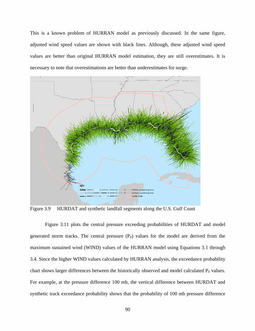
90

This is a known problem of HURRAN model as previously discussed. In the same figure,

adjusted wind speed values are shown with black lines. Although, these adjusted wind speed

values are better than original HURRAN model estimation, they are still overestimates. It is

necessary to note that overestimations are better than underestimates for surge.

Figure 3.9 HURDAT and synthetic landfall segments along the U.S. Gulf Coast

Figure 3.11 plots the central pressure exceeding probabilities of HURDAT and model

generated storm tracks. The central pressure (P0) values for the model are derived from the

maximum sustained wind (WIND) values of the HURRAN model using Equations 3.1 through

3.4. Since the higher WIND values calculated by HURRAN analysis, the exceedance probability

chart shows larger differences between the historically observed and model calculated P0 values.

For example, at the pressure difference 100 mb, the vertical difference between HURDAT and

synthetic track exceedance probability shows that the probability of 100 mb pressure difference

91

is 10% more in synthetic storms case than historical case (Figure 3.11). This means that original

synthetic model creates stronger storms than historical storms. Figure 3.13 also confirms that

computed wind speeds of synthetic storms are stronger, as demonstrated by the exceedance

probability of central pressure values of hurricanes along the northern Gulf of Mexico Coast.

Figure 3.10 Wind speed cumulative probability comparison plots at each gate (historical data is

red color, adjusted synthetic data is black color, and synthetic data is blue color)

Figure 3.12 shows the cumulative probability charts of central pressure values for both

historical data and calculated from adjusted synthetic model. The central pressure data shows

similar trends except gates 4, 8, 12 and 16. The insufficient number of historical landfalling

storms may cause these differences. There are 172 historical storms with observed central

pressure values passing through 16 gates. On the other hand, there are 5471 landfalling synthetic

storms in the same region. The difference in the number of storms makes the comparison

difficult. For example, Gate 8 has only 5 historical storms; on the other hand, it has 132 synthetic

storms.

92

Figure 3.11 Exceedance probability chart for pressure of HURDAT versus synthetic storms

(original synthetic model)

Figure 3.12 Cumulative probability plot at each gate (historical data is red color, adjusted

synthetic data is black color)

93

Figure 3.13 illustrates the exceedance probability of wind speed for HURDAT (blue

color), original HURRAN (orange color) model, and modified HURRAN (red color) model

estimations. Based on this figure, the track propagation methodology that utilize modified

HURRAN model generates weaker synthetic tropical cyclone tracks than unmodified HURRAN

model. This indicates that the modified HURRAN model performs better than the original

HURRAN model in speed calculations. Also, the Figure 3.14 outlines one extreme historical

storm more than 160 knots wind speed. This extreme storm is a ten thousand year event.

The exceedance probability values for segment headings are also calculated (Figure

3.14). This graph illustrates the entire fidelity of headings through entire track that the historic

and synthetic storm paths are similar. This figure indicates that model under performs for

looping storms segments where directional change more than 22.5 degrees on either side of

normal heading as mentioned in Table 3.2. Similarly, Figure 3.15 shows the storm tracks heading

at gate locations.

Figure 3.13 Exceedance probability chart of wind speeds from model created synthetic tracks

and recorded historical storm tracks

94

Figure 3.14 Exceedance probability chart for heading of observed and modeled storms.

Figure 3.15 Exceedance probability chart at each gate for heading of observed and modeled

storms (blue lines HURDAT tracks, red lines synthetic tracks)

95

Based on the analysis results, the track propagation methodology that utilizes the

unmodified HURRAN model generates accurate synthetic tropical cyclone tracks but with

stronger storms values, such as wind speed, and central pressure. This problem is partially

addressed with implementation of segment wind speed correction within the track propagation

framework. The introduced equations in this module are used to reduce wind speed and pressure

under/overestimation. With this correction module, synthetic track propagation framework is

repeated to correctly estimate storm parameters for reliable storm surge estimation (Chapter 4).

3.7 Summary

This chapter starts with the review of existing storm track forecasting/prediction models

for the North Atlantic Basin. Thirty-six different storm forecast and non-forecast models are

investigated to identify key parameters of atmospheric conditions for storm generation, statistical

and non-statistical methods for solving/modeling of storm event, and performance characteristics

of existing models. Several key parameters are identified that are required for implementation of

synthetic storm track generation model. These identified parameters are latitude, longitude,

central pressure, date and time, wind speed, radius of max winds, and Holland B.

The synthetic storm track methodology framework is outlined in this chapter. This

methodology framework consists of three main modules; namely, synthetic genesis location data

as an input, track propagation as a computation framework, and synthetic track data as an output.

In the track propagation module, the synthetic tropical cyclone simulation process starts with the

selection of a synthetic genesis location. Then, the track propagation calculations are executed.

The calculated results are exported to suitable formats for future analysis. These results are

stored in an ASCII file format which is utilized in Chapter 4 and a geo-database which will be

discussed in Chapter 5.

96

The track termination and candidate segment selection modules are modified in this

implementation by utilization of program libraries of GIS. This modification reduces the

positional error compounding due to projections, and related map projection conversions.

Second, the implemented wind speed and central pressure corrections result more accurate

synthetic storm parameter values than the original HURRAN model. In addition, the HURRAN

model is enhanced with inclusion of storm intensity parameters (e.g. radius to maximum winds,

Holland B parameter), into the model output for each track segment. The computational formulas

for storm intensity parameters were developed a later date than the development of the

HURRAN model (e.g. Holland B introduced in 1980 which is a key parameter for estimation of

storm surge elevation in Chapter 4). These refinements represent a significant improvement to

the original HURRAN implementation by enabling the simulation of the life cycle of a hurricane

from genesis to dispersion.

The accuracy and results of implemented synthetic track model has been evaluated by

comparing historical tropical cyclone data in GOM. The comparison of track heading and

location results show that generated synthetic storm tracks are highly similar to the historical

storm tracks in direction. Also, the calculated wind speed values from modified track

propagation model are closer to the historical wind speeds than calculated wind speed values

from unmodified HURRAN. The central pressure values are better because of adjusted wind

speeds utilization. The modifications introduced in segment smoothing module results in

increase in accuracy of calculated wind speed and related storm strength parameters. As a result,

this translates improved the storm surge levels calculations in Chapter 4.

97

CHAPTER 4: STORM SURGE SURFACE


The accurate estimation of storm surge elevations along coastal regions is important to

facilitate informed and appropriate decisions and planning. Within the context of the overall goal

of this dissertation, the purpose of this chapter is to investigate existing methods utilized for

storm surge estimation, as well as the key storm parameters used in existing Ocean Circulation

Models (OCMs) in order to create synthetic storm surge surfaces from a hybrid model, that

combines a Joint Probability Method (JPM) and an Artificial Neural Network model (ANN) with

key historical and synthetic tropical cyclone tracks. Existing OCMs are investigated to design a

simple, high-resolution storm surge estimation approach using key storm parameters (e.g.

landfall coordinates, date, time and wind speed). The first section of this chapter reviews existing

OCMs with a focus on surge estimation models for the North Atlantic Basin, with special

emphasis on models that are used in the forecast and hindcast processes of tropical cyclones. The

second section outlines the development of a storm surge estimation methodology utilizing a

neural network (NN) model developed with the identified key storm parameters. In this section,

the effects of the identified parameters on storm strength and coastal storm surge are examined.

In addition, the contribution and interaction of the identified parameters are investigated for

estimation of storm surge elevation. The final section gives the data analysis and case study

results of the developed methodology. Synthetic storm surge surface model results created by

hybrid ANN model from this chapter will be combined in a geodatabase framework (Chapter 5)

for seamless integration with both synthetic and historical storm genesis (Chapter 2) and track

data (Chapter 3) model results.

98

4.2 Introduction

Communities in coastal regions are vulnerable to storm surge caused by tropical

cyclones, especially along the northern Gulf of Mexico. Strong tropical cyclones can cause

coastal inundation, resulting in property damage and loss of life. Since the 1970s, several

numerical methodologies to determine storm surge elevations from coastal tropical cyclones

have been developed. These models are referred to as ocean circulation models (OCMs) (Bryan

and Cox 1972). OCMs generally contain atmospheric and oceanic modules to handle the

different aspects of tropical cyclone modeling applications. Atmospheric modules compute storm

track propagation (e.g. GFDL) whereas oceanic modules compute wind induced surge elevations

(e.g. ADCIRC). Chapter 3 provides a listing of existing storm track forecast models based on

mathematical modeling approaches and Appendix C provides an overview of these models. This

chapter focuses on the ocean components of the circulation models, specifically coastal

inundation (surge) modeling from tropical cyclones.

Since the inception of OCMs, many inundation estimation models for coastal regions

have been developed (e.g. Jelesnianski et al. 1992, Luettich et al. 1992, Smith et al. 2011, Smith

et al. 2012, Taylor 2008). Existing coastal storm surge estimation methodologies follow

deterministic, statistical, or hybrid modeling approach. In the deterministic approach, complex

hydrodynamic equations are solved to estimate surge elevations (Blumberg and Mellor 1987,

Chen et al. 2003, Hallberg 1995, Jelesnianski et al. 1992, Luettich et al. 1992, Smith et al. 1992).

The drawback of this approach is the time and cost required to obtain results. In the statistical

modeling approach, estimation of storm surge elevations are computed by using historical surge

observation data (e.g. Pirazzoli and Tomasin 2007, Taylor and Glahn 2008, Walton 2000). The

drawback of this approach is the limited number of historical records and the spatial distribution

of the surge observation locations (Landsea et al. 2008, Walton 2000). For example, the most

99

comprehensive storm surge database contains clustered points of observation records for 195

events for the US Gulf Coast (Needham and Keim 2011), although this dataset is currently being

expanded. Finally, the hybrid modeling approach combines deterministic modeling with

statistical modeling to create an ensemble of surge records (e.g. Smith et al. 2011, e.g. Smith et

al. 2010). This approach utilizes deterministic storm surge simulation results and historical storm

surge data for the statistical surge estimation. This methodology is very time consuming and

costly to obtain results.

A new synthetic hybrid coastal storm surge estimation methodology is proposed for

storm surge elevation estimation based on the combination of stochastic and deterministic

methodologies. In the proposed methodology, the Joint Probability Method (JPM) is used as a

stochastic methodology to identify significant key storms track and related parameters (e.g.

storm heading, coordinates). The simulation results of these identified storms are used as input

for the development of a synthetic storm surge database for deterministic calculations. In this

study, the storm surge results from 40 personally simulated and 152 simulations obtained from

the National Flood Insurance Study (NFIS) (Niedoroda et al. 2008b, Toro et al. 2007, Toro et al.

2010b)for southwestern coastal Louisiana are utilized. The NFIS study dataset is used to reduce

computational time required for the ADCIRC model simulations. The storm surge simulation

results from the NFIS are a collection of the significant tropical cyclone tracks and relevant

parameters that were identified through the JPM analysis. The simulated storm surge elevation

surfaces and these identified parameters are used in the development of the NN model. The

proposed approach requires minimal operational cost and computational time and can be used to

calculate storm surge elevations for a specific tropical cyclone on a desktop computer within

minutes.

100

4.3 Background of JPM and NN Models for Storm Surge Estimation

Deterministic methods (Appendix E) of storm surge estimation use simplified depictions

of sea levels, which are represented by crucial contributing factors (e.g. storm tide, astronomical

high tide). These factors do not require long-term observational data for calculation. Conversely,

statistical methods require the existence of long-term historical data. This is a limitation of

statistical methods because of the scarcity of long-term records. However, statistical methods are

more reliable in estimating storm surge elevations due to the inclusion of historical variations.

Additionally, statistical approaches calculate storm surge elevation as a random variable instead

of as a fixed storm surge elevation. In other words, the storm surge elevation can take a set of

possible values due to the uncertainty in storm parameters, such as winds speed and central

pressure. Therefore, the quantification of storm surge elevation requires an understanding of

contributing storm parameters and estimation of the extreme values of those parameters.

Empirical statistical techniques (EST) and joint probability methods (JPM) are examples

of statistical approaches. EST and JPM are similar in their estimation process; however, the

datasets they use differ. In JPM, historical and synthetic storm surge datasets are used without

any modification. In EST, the dataset is extended using a bootstrap method (Scheffner et al.

1999). There is only one probabilistic surge model that uses EST: pSurge (Taylor and Glahn

2007, Taylor and Glahn 2008). The primary disadvantage of EST is that the interrelationship

between parameters is taken into account; therefore, the extreme surge elevation cannot be

estimated (Scheffner et al. 1999, Toro et al. 2010b). For this reason, a JPM type methodology is

more appropriate for storm surge elevation estimation from a limited number of key extreme

samples, which is the approach utilized in this study. JPM methodologies have been utilized in

recent storm surge studies conducted for Louisiana and Mississippi coastal regions (Niedoroda et

al. 2010, Niedoroda et al. 2008a, Toro et al. 2010a, Toro et al. 2009, Toro et al. 2010b).

101

Historically, the determination of maximum storm surge elevation estimation consists of

the analysis of a statistically significant number of events for water levels, which are combined

tide elevation, surge, and wave setup above mean sea-level (Ackers and Ruxton 1975, Butler et

al. 2007, Führböter 1979, Graff 1981, Lennon et al. 1963, Walton 2000). A maximum water

level for related modeling, such as return period and maximum envelope of water (MEOW), is

generally calculated by one of two extreme value distributions: the Gumbel Extreme Value Type

1 (GEV1) model (Gumbel 1954) or the Generalized Extreme Value (GEV) model (Jenkinson

1969). In recent years, extreme water level estimation modelers have attempted to separate the

deterministic and stochastic components of storm surge levels into the deterministic astronomical

tide and the stochastic meteorological surge component (Coles and Tawn 1990, Flather 1987,

Flather et al. 1998, Myers 1970, Tsimplis and Blackman 1997). The separate analysis of these

two independent components of storm surge simplifies the modeling. The astronomical tide is

easily calculated from previously observed tidal values at a location and can be excluded from

unknown variables in probabilistic calculation. Furthermore, in this study, the deterministic

storm surge calculation methodology is separated from statistical identification of probabilistic

calculations and key (extreme) storm tracks and related parameters for computational

simplification. The uncertainty in storm surge elevation is addressed with joint probability

modeling (JPM). For the deterministic storm surge elevation calculations, a Neural Network

(NN) approach is used.

Neural Networks (NNs) are, in statistical terms, a group of flexible nonlinear regression

models used for discrimination, reduction, and estimation of data in nonlinear systems

(Kretzman 1994, Sarle 1994). The aim of NNs is to determine the relationships between input

and output such that the differences between the output values and target values are minimized.

102

Appendix E provides a more detailed description and visualization of NNs. In this study, the

neural networks are referenced with the adjective “artificial” to distinguish the utilization for

data analysis. An artificial neural network (ANN) is one of the methods used in computational

intelligence models. The ANN is commonly used in development of data-driven models and are

desirable for usage in soft computing due to tolerance for imprecision and uncertainty in data

(Haykin and Haykin 2009). In addition, ANNs are common in data mining applications for

preparation, reduction, and finding dependency rules from data. In this study, the ANN is utilized

as a module to create the proposed predictive storm surge methodology.

Since the late 1986s, ANNs have been implemented for various problems in many fields

(Tissot et al. 2001, Tissot et al. 2004). For example, the time series-related prediction problems

are solved for hydrological applications (e.g. Huang et al. 2007). Sztobryn (2003) applied an

ANN methodology in hydrological forecasting of sea levels with respect to winds in Texas. The

results of ANN models are comparable with other forecast methodologies and observations of

actual sea levels (Huang et al. 2007, Lee 2009, Sztobryn 2003). Similarly, Lee (2009, 2006) and

Tseng et al. (2007) demonstrated the effectiveness of ANNs in forecasting storm surge from

tropical cyclones in Pacific. These studies utilized measurements from multiple tide stations as

inputs to the ANNs. In the North Atlantic, Siek and Solomatine (2010) illustrated that ANN

estimation results are compatible with chaotic model results for short-term storm surge

predictions (e.g. Siek and Solomatine 2010). Huang et al. (2007) and de Oliveira et al. (2009)

concluded that ANNs can be applied in operational forecast services. Based on these ANN

implementations, a multilayer perceptron version of an ANN model (a multivariate simple

nonlinear regression model) is implemented for storm surge level estimation in this study.

Although the proposed model does not use any time series data from tide gauges, the model

103

incorporates independent variables (e.g. coordinates, central pressure, Holland B and radius of

maximum winds) as inputs from synthetic or historical tropical cyclone tracks.

4.4 Storm Surge Estimation Methodology Framework

The proposed methodology is a GIS-integrated, fast-running, ANN-based non-forecast

methodology for computing storm surge surfaces. The implemented methodology combines both

JPM and ANN models to determine stochastic parameters and compote deterministic surge

elevations from related stochastic parameters, respectively. This methodology reduces the

shortcomings of existing models, such as long computation time and costly computer hardware

requirement. OCMs are described in detail in Appendix E (e.g. ADCIRC, FVCOM); therefore,

this section discusses only the implemented methodology.

The proposed process of the tropical cyclone surge estimation methodology consists of

three stages (Figure 4.1): 1) tropical cyclone track data as input, 2) storm surge surface

estimation, and 3) estimated storm surface as output. The genesis and track data creation and

historical records are explained in Chapters 2 and 3. These data are used as inputs for the first

stage. The second and third stages are explained in following sections. The focus is the

development of the storm surge estimation framework that combines JPM and ANNs.

This framework requires the synthetic and historical tropical cyclone tracks as an input

for the Joint Probability Method (JPM) procedure. The significant tropical cyclone tracks and

key parameters effecting storm surge are identified using JPM for the NFIS (Toro et al. 2010b).

Since the NFIS study covers the same region, the NFIS study results are verified with historical

tack data. The additional 40 significant tracks with key parameters are simulated with the

ADCIRC model. The storm surge surfaces from the NFIS and additional simulations are utilized

for this study. Next, these data are converted to a computation matrix by utilizing image to data

conversions, preserving geo-reference information. The ANN is trained using the computation

104

matrix created from simulated storm surge surfaces, resulting in activation functions. These

computed activation functions are utilized to estimate storm surge levels. The computed results

are exported to a format for storage in the geo-database.

Figure 4.1 Storm surge surface methodology framework

Study Area 4.4.1

The study area for the tropical cyclone surge estimation methodology between 92° 00’

0’’W and 94° 30’ 00’’W longitudes, and between and 29° 00’ 00’’N and 31° 00’ 00’’N latitudes

in southwestern coastal Louisiana (Figure 4.2). The study area is outlined with a blue rectangle

in the figure. This area is delineated based on two major considerations: 1) physical and

meteorological factors, and 2) availability of historical storm track and surge data.

Data Sources 4.4.2

The storm surge estimation methodology utilizes both tropical cyclone track and storm

surge elevation datasets. The historical tropical cyclone track dataset (HURDAT) is utilized to

identify significant storms and related track parameters. For example, the important storm

forward movement directions are north-northwest, northwest, and north for the southwestern

Louisiana. In the utilized HURDAT database, there are 1,457 tropical cyclone records.

105

Figure 4.2 Storm surge model extent

The storm surge scenarios from the NFIS are identified for 152 cases using the three

identified headings within the study area. The National Flood Insurance Study dataset contains

of storm surge surfaces in JPEG file format for 152 key events simulated with the ADCIRC

model. Additional storm surge simulations are derived from 40 storm scenarios using the

ADCIRC model. Therefore, the total number of storm surge surfaces utilized in this study is 192.

These surge elevation datasets are utilized to create surface estimation functions within the ANN.

In addition, these ADCIRC model simulated storm surge elevations are used to populate a

geodatabase table for synthetic storm surge elevations. The utilization of the geodatabase

provides flexibility for identification of surge and related tropical cyclone tracks. For example,

Hurricane Katrina surge and tracks can be extracted from related tables of the geodatabase.

Another advantage is the preservation of spatial information and related parameters. For

example, during the creation of a JPEG file, accuracy of cell values and projection information is

lost. This loss of information also occurs related to colors. For example, the display of surge

elevation values changes due to dithering effects.

106

4.5 Storm Surge Surface Methodology

JPM is selected for implementation since it considers the variability of the key storm

parameters affecting the surge elevations (Toro et al. 2010a). Furthermore, JPM provides means

to minimize the resources needed for the model development (Toro et al. 2007, Toro et al.

2010b). For example, it is preferable to run 192 ADCIRC simulations for JPM identified key

tracks instead of 1457 tracks in the historical dataset. The JPM identifies the following key storm

parameters: storm heading, storm central pressure, radius of maximum wind speed, forward

speed, landfall location, and approach angle. Based on the JPM results, it is statistically possible

to represent tropical cyclone storm surge with these 192 storm scenarios. The detailed

description and formulation of these variables is illustrated in the next section.

JPM Sampling from Historic Track 4.5.1

Toro et al. (2007, 2010b) explain in detail the JPM methodology for identifying tropical

cyclones and related parameters that are significant for coastal storm surge. This same

methodology is used for identifying tropical cyclone tracks for the NFIS. In this study, the only

difference is the addition of Holland B parameter. Figure 4.3 illustrates the parameters used in

the JPM calculation.

Storm Surge Surface Simulations with ADCIRC 4.5.2

The NFIS study contains 337 storm surge surfaces for Louisiana. 152 out of 337

simulations are related to the study area. Ideally, it is preferable to obtain original ADCIRC

simulation results (fort files). For this study, the original ADCIRC simulations results were not

available, so the NFIS surge surfaces for the simulated tropical cyclones were obtained as JPEG

files. This file format is converted to a matrix structure for computational ease (Appendix G).

Forty additional historical hurricane tracks are simulated with ADCIRC to obtain additional

107

storm surge surfaces. The geodatabase table for the synthetic storm surge surfaces is populated

using the results of the 192 tropical cyclone track simulations.

Figure 4.3 Characterization of storm at coast (Toro et al. 2007)

Converting Simulation Results to Computation Matrix 4.5.3

The surge surfaces from each storm are converted a computation matrix. This matrix is a

multi-dimensional array containing surge surface elevations with storm track parameters. The

surge elevations are extracted from the NFIS surge JPEG images. The conversion from JPEG file

format to the computation matrix is explained in Appendix G. The storm parameters of interest

are central pressure, Holland B, RMW, and coordinates values at landfall and 24-hour prior to

landfall. These parameters are obtained from identified storm track cases.

The computation matrix provides a means to combine track and surge snapshots. The

creation of this matrix allows improvement for the ANN training. Furthermore, this derived

structure incorporates JPM-identified parameters into a structure as independent variables for the

ANN. For example, the RMW and Holland B parameters are represented as a product of each

other at landfall and 24 hour prior to landfall.

108

Artificial Neural Network Training Methodology 4.5.4

For the simplification of the problem and generalization of the described equations, the

following assumptions are made:

1. The hurricane category is known,

2. The landfall location is known,

3. The hurricane speed is known,

4. The direction of movement is known,

5. Radius of maximum winds and wind field extent are known,

6. Storm surge is insignificant outside the defined region.

The surge computation matrix is created by query result from the storm surge database

with matching key tropical cyclone parameters (e.g., central pressure, latitude and longitude).

This matrix is used to perform multivariate simple nonlinear regression. The result of the

regression analysis is the estimation of the activation function for the ANN. For the training of

the ANN, a surge surface database with 192 events is used. The polynomial functions (H1, H2,

and H3) in Figures 4.4 and 4.5 are activation functions of the ANN.

Artificial Neural Network Model 4.5.5

Artificial Neural Network modeling can be used to predict the response variable. During

the training of the ANN, the functional dependency between response and input variables is

captured (SAS 2012). This response surface may (or may not) represent actual interaction

between the tropical cyclone parameters. Therefore, JPM-identified parameters are utilized for

capturing a better response surface from the ANN. Figure 4.4 gives a diagram of the Artificial

Neural Network used in this study. The green filled circles represent the activation functions,

which are in a hidden calculation layer used in the estimation of surge elevation (Z). The hidden

layer equations and the equation to predict Z are provided in Figure 4.5. Input parameters are:

109

Dist = the distance between a point and storm eye (meter)

X distance = longitude (decimal degree)

Y distance = latitude (decimal degree)

P0 = pressure value recorded at landfall (mb)

P24 = pressure value 24 hours prior to landfall (mb)

R0 H0 = multiplication of Holland B and the radius to maximum winds computed at landfall

(dimensionless)

R24 H24 = multiplication of Holland B and the radius to maximum winds computed 24 hours

prior to landfall (dimensionless)

Figure 4.4 Artificial neural network diagram

The combination of radius of maximum wind (R0 and R24) and Holland B (H0 and H24)

parameters provides insight into tropical cyclone strength and potential for coastal storm surge

110

levels. In most studies, these parameters are considered independently from each other (Smith et

al. 2011, Smith et al. 2012, Vickery et al. 2000c, Vickery and Wadhera 2008). The combination

of these parameters gives better estimation compared with separate utilization in ANN modeling.

Figure 4.5 Neural network structure and surge elevation estimation equation

Storm Surge Surface Output 4.5.6

The computed surge matrix is converted to a geo-tif file format, which is a lossless image

file format with associated geo-referencing information. The geo-tiff file data do not change

during file write operations. Geo-giff format is also a common format for GIS, and the exported

surge surface file is stored in geodatabase. The details of geodatabase are explained in Chapter 5.


Artificial neural network modeling (ANNM) data analysis is performed using the

synthetic storm surge data described in Section 4.4.2. The dataset is divided into training data,

used in the development of the estimation process, and validation data, used for the confirmation

study. Surge elevations and corresponding parameters are extracted from the NFIS images as

data points. The number of surge elevation data points used in the ANN development is 22,909

after the elimination of non-data image cells (e.g. dry land areas are eliminated). About 80% of

these data are used as training data and the remaining are used as validation data (Fausett 1994).

111

Training And Validation Data Sets Fits 4.6.1

A trial and error procedure is applied to estimate the number of training data to maximize

the coefficient of determination (R2) of Zactual vs Zestimated (SAS 2012). Figure 4.6 and 4.7 provide

the training and validation data sets fits and Table 4.1 provides the fit statistics for training and

validation data sets. The training and validation dataset fits show good agreement. Based on the

validation dataset statistics, the coefficient of determination (R2) is slightly higher and the RMSE

is slightly less than for the training data fit statistics. Also, plots of the residual versus the

predicted values (Figures 4.8and 4.9), show smaller errors in the validation set. This confirms

that the developed neural network model is a reasonable model to estimate storm surge

elevations for the study area.

Table 4.1 Fit statistics of training and validation data sets

Measures Training Validation

R2 0.818533 0.8240159

RMSE 1.4932628 1.4778735

Mean Abs Dev 1.0551165 1.0544174

-LogLikelihood 27795.364 13817.668

SSE 34056.251 16677.864

Sum Freq 15273 7636

Figure 4.6 Actual versus predicted plot of training data set

112

Figure 4.7 Actual versus predicted plot of validation data set

Figure 4.8 Residuals by predicted plot for training data set

Figure 4.9 Residuals by predicted plot for validation data set

113

Prediction Profiler Plot 4.6.2

Since the training and validation dataset fits (Figures 4.6 and 4.7) are acceptable, the

profiler plot (Figure 4.10) is evaluated to determine the sensitivity of the each variable. In Figure

4.10, the x-axis represents the variables used in the ANN and the y-axis represents the

corresponding surge elevation, Z, calculated from the ANNM. In this figure, the red dashed lines

demonstrate a specific case and the variables’ values are indicated by red numbers under the x-

axis. For this specific case, the corresponding estimated surge elevation, Z, is approximately 7.24

feet, shown to the left of the y-axis. In this figure, black lines show the changes in elevation (Z)

if the variable is changed while the other variables remain constant.

In order to understand the effects of the various storm parameters on storm surge

elevation estimation, the profiler plot (Figure 4.10) should be investigated. When the first row of

the prediction profiler plot is considered (Xdistance, Ydistance, Dist variables), the neural network

model produces similar trends compared with an actual tropical cyclone surge trend. In the Xdist

profile plot cell, the surge elevation decreases as the distance from the eye of the tropical cyclone

increases. Conversely, the Ydist plot indicates that surge levels increase gradually as the storm

approaches the coastline (landfall). The Dist plot shows the change in surge elevation change as

the observation cell moves farther away from storm eye. For the central pressure of storm, there

is a reverse relationship between 24 hour prior to landfall (P24) and at landfall pressure change

(P0). If the central pressure (P0) closes to ambient pressure at landfall, the storm surge elevation

increases. If the central pressure (P24) is close to ambient pressure, which is 1013 mb, the storm

surge elevation decreases. In other words, if the pressure 24 hours prior to the landfall is lower

(stronger storm), the tropical cyclone created surge levels is higher in coastal areas (Simpson and

Pielke 1975). Similarly, there is an inverse relationship between multiplications of the radius of

maximum winds and Holland B values at landfall (R0 H0) and 24 hour prior to landfall (R24

114

H24). In other words, the tropical cyclones with larger wind effected area generates higher storm

surge in coastal zones because winds push more water toward the land (Simpson and Saffir 2007,

Simpson and Pielke 1975). This characteristics change direction causing decrease in surge levels

at the right side of storm eye because of counter-clock wise rotation of storm. All of the observed

trends are consisted with historical data and this developed ANN is tested with a previous case

study.

Figure 4.10 Prediction profiler plot

115

Analysis of Residuals 4.6.3

An analysis of storm surge elevation residuals is performed and the results are provided

in Figure 4.11. The lower portion of the plot provides the storm surge elevation residual

histogram and the superimposed theoretical normal distribution is shown with a red curve. The

upper portion of the plot provides the normal quantile plot of storm surge elevation residuals. In

this plot, the scales outside and inside of the plot provide the normal quantile and probability

values, respectively. The points show the individual residuals and the red solid line provides the

theoretical distribution of the normal plot for the specified mean (-0.0011) and variance (1.4929).

The 95% confidence interval is the area between the two red dashed lines.

Based on Figure 4.11, the residual distribution is similar to the normal distribution. The

majority of residuals (between 0.02-0.98) follow the red line. The values outside the interval of

0.02 and 0.98 are extreme values. Estimated mean and standard deviation of the residual

distribution with 95% confidence intervals are given in Table 4.2. The mean of the error

distribution is very close to zero and the 95% mean confidence interval includes zero. This

satisfies the residual analysis assumption, where residuals should be normally distributed with a

mean value of zero. This residual analysis and high R2 demonstrates the good performance of

prediction model.

4.7 ANN Model Case Studies

To confirm the estimation accuracy of the developed ANNM, a case taken from the

National Flood Insurance Study is conducted. For the case study, surge levels given in Figure

4.12 are used. By using the developed Artificial Neural Network model, the surge levels are

calculated for every point of mesh (500 m by 500 m grid) over the study area. The input

parameters of P0, P24, R0, R24, H0, and H24 are obtained from the track data of Storm 206 (Figure

4.12) for this study.

116

Table 4.2 Parameter estimation of error distribution

Confidence Interval

Parameters

Estimate

Lower 95%

Upper 95%

Mean, μ

-0.0011

-0.0204

0.0183

Std. Dev., σ 1.4929

1.4794

1.5067

Figure 4.11 Z error distribution

117

Figure 4.12 Surge test case (storm 206, max water level (feet))

Figure 4.13 Comparison of measured and calculated storm surge elevations using the artificial

neural network

118

Figure 4.13 gives the comparison of the extracted (measured) data from the ADCIRC

simulation result (blue circles) and the calculated data from ANN (red pluses) for Storm 206.

Based on this figure, the trend of the calculated data is similar to measured data. For example,

near the storm landfall location, the storm surge elevations obtained from NFIS and ANN are 11

ft and 9.8 feet, respectively, a difference of approximately 10.9%. Considering the uncertainty of

the ADCIRC model of 2-5% (van Heerden et al. 2007), the maximum error of the developed

ANN model is 16%. This indicates that the performance of ANN is better that SLOSH model (±

20%). This case study confirms that the developed ANNM is suitable for storm surge elevation

estimation provided that key storm parameters are known.

After testing the artificial neural network model, a probabilistic estimation study is

conducted. Since available historical datasets are too limited to conduct a probabilistic

estimation, synthetic storms generated from simulations are used to estimate the distribution of

storm parameters. All distributions are tested and the best distribution is chosen with the

comparison of Akaike Information Criterion with bias adjustment (AICc) (SAS 2012). The lower

AICc gives the best fit. Figure 4.14 provides the histogram of historic pressures recorded at

landfall (P0) (HURDAT records along Louisiana coastline) and the summary statistics. The AICc

analysis (Table 4.3) shows that the best distribution is Weibull with scale and shape parameters

of 957.317 and 61.5326, respectively. Figure 4.14 shows the best fit Weibull distribution with a

blue line.

Figure 4.15 gives the Diagnostic plot of P0. In this plot, the red solid line provides the

theoretical Weibull distribution for the specified scale and shape parameters. The area between

the two red dashed lines provides the 95% confidence interval. The goodness-of-fit Cramér-von

Mises W Test, which compares the theoretical and empirical distributions, is provided to the

119

right of the plot. This test results in a P-value is greater than 0.05, which indicates that the

Weibull distribution fit is acceptable for pressures.

Figure 4.14 Histogram of P0

Table 4.3 Distribution comparison for P0

Distribution Number of Parameters -2*LogLikelihood AICc

Weibull 2 224.326202 228.847941

Extreme Value 2 224.326202 228.847941

Normal 2 225.894079 230.415818

Gamma 2 226.004464 230.526203

LogNormal 2 226.072724 230.594463

Johnson SI 3 224.070833 231.161743

GLog 3 225.874358 232.965267

Johnson Su 4 225.875194 235.779956

Normal 2 Mixture 5 222.911208 235.911208

Normal 3 Mixture 8 213.644364 238.114952

Exponential 1 408.455962 410.622628

Figure 4.15 Diagnostic plot of P0

120

Figures 4.16, 4.18 and 4.20 provide the distribution and the best distribution fit of

pressure 24 hours prior to landfall (P24), multiplication of Holland B and radius to maximum

winds at landfall (R0×H0) and multiplication of Holland B and radius to maximum winds 24

hours prior to landfall (R24×H24), respectively. The best distribution fit for P24 and R0×H0 is the

Weibull distribution and the best fit for R24×H24 is the lognormal distribution. Figures 4.17, 4.19

and 4.21 provide the diagnostic plots of these variables. All p values are greater than 0.05,

indicating that all distribution fits are acceptable.

Figure 4.16 Histogram of P24

Figure 4.17 Diagnostic plot of P24

121

Figure 4.18 Histogram of R0×H0

Figure 4.19 Diagnostic plot of R0×H0

Figure 4.20 Histogram of R24×H24

122

Figure 4.21 Diagnostic plot of R24×H24

To find the probabilistic surge level, Monte Carlo Simulation is used. Five thousand

(5,000) samples are randomly chosen from the above specified distributions and surge levels are

calculated using the developed neural network model for the selected case location. Figure 4.22

provides the histogram and statistics of calculated surge levels. Estimated mean surge elevation

and standard deviation are 8.33 feet and 1.04 feet, respectively.

Figure 4.22 Histogram of surge level

Figure 4.23 gives the cumulative distribution of calculated surge elevations. Based on this

figure, the cumulative distribution value increases sharply at the mean value, indicating a highly

confident estimation.

123

Figure 4.23 Cumulative distribution of surge level

4.8 Summary

In this chapter, existing storm surge models are examined to identify the key storm

parameters affecting storm surge elevation. The identified parameters are storm coordinates

(latitude and longitude), central pressure at landfall and 24 hour prior to landfall, radius of

maximum winds, and Holland B value. An ANNM was developed to identify the relationship

between storm surge elevations and the identified key variables for southwestern coastal

Louisiana by utilizing historical and synthetic key storm parameters. The synthetic dataset was

selected from the Flood Insurance Study (FIS), as these data are the result of a JPM analysis,

integrating both influencing factors and their associated probabilities into the storm surge

simulations.

The dataset was divided into a training dataset to develop the relationships between storm

surge elevation and key parameters, and a validation dataset to test the goodness of fit for the

developed ANNM. For both datasets, measured and estimated storm surge cross plot statistics

and residual analyses indicated that the developed ANNM is suitable for storm surge estimation.

Additionally, the profiler plot of the ANNM is consistent with storm surge theory and historical

observations. After the ANN development, a case study taken from the NFIS was conducted to

124

demonstrate the similarity of estimated and simulated storm surge elevations. The case study

confirmed that the performance of the developed ANNM provides an estimate with lower error

that the published error ranges for the SLOSH model.

The main advantages of the developed model are that it is computationally less

demanding and suitable for probabilistic storm surge elevation estimation. A Monte Carlo case

study was conducted to assess the performance of the ANNM. Probabilistic storm surge

elevations can be obtained through Monte Carlo simulation to account for uncertainty in the key

parameters. The standard deviation of the estimated storm surge elevation from this case study is

low, indicating a highly reliable estimation from the developed ANNM.

125

CHAPTER 5: TROPICAL CYCLONE TRACK AND STORM SURGE GEODATABASE

INTEGRATED MODEL


This chapter focuses on the organization and framework of a geodatabase that will store

both historical and synthetic tropical cyclone genesis and track locations, their intensity-related

parameters, and storm surge elevation data for use in computations. Within the context of the

overall goal of this dissertation, the purpose of this chapter is to investigate existing datasets and

data storage practices to develop a more efficient data storage framework that can be used to

integrate all available vector and raster datasets seamlessly. Existing database management

systems are investigated to design a geodatabase to store both spatial and non-spatial data

components. The first section of this chapter provides a review of existing modern tropical storm

track and storm surge databases. The next section outlines the integrated geodatabase framework

development. The final section discusses the advantages and disadvantages of the developed

geodatabase framework against existing database frameworks.

5.2 Introduction

There are a limited number of historical tropical cyclone track and storm surge elevation

observation records in the North Atlantic Basin for use in statistical modeling. Also, there is no

tropical cyclone track and storm surge surface elevation data integrated geodatabase for

modeling in the North Atlantic basin (Needham and Keim 2011). The main shortcoming of the

separation of tropical cyclone tracks and storm surge-surface information is the difficulty in

association of storm track parameters with affiliated storm surge elevations over the event’s

spatial domain utilizing a traditional database structure. Furthermore, the collected historical

storm surge information is a combination of discrete data observations that form a sparse

collection of locations and surge elevations measured at interior landmarks. For example, the tide

126

station measurements on a bridge, the surge debris line on a hillside, or the high water mark on a

house wall are three kinds of surge elevation indicators and surge data collection sites. These

discrete data locations hinder effective and accurate visualization and statistical modeling of

storm surge. To overcome these limitations, it is necessary to utilize tropical cyclone tracks as

discrete locations and storm surge elevation data as continuous surfaces. Therefore, this chapter

proposes a solution for coupling synthetic and historical storm track information with storm

surge records in a geodatabase for identifying the association between key storm parameters and

surge elevation and improving storm track and surge visualization.

In order to understand the state-of-the-art requirements for tropical cyclone track and

surge databases, the published literature focusing on parameters used in storm forecasting

models was reviewed. After evaluating existing records of storm tracks, a relatively simple and

easy to use storm track and surge elevation integrated geodatabase design is proposed. The

proposed single-user (Microsoft Access personal) geodatabase runs on a desktop environment.

However, the same schema is applicable to multi-user large-scale enterprise relational database

management system (RDMS) platform, such as Microsoft SQL Server and IBM DB2.

In addition to historical tropical cyclone records, simulated (synthetic) tropical cyclone

track data are stored in the geodatabase. This provides a means to expand the historical track

datasets with statistically representative synthetic tracks. Another advantage of the geodatabase

is that storm track information is coupled with storm surge data (stored as tables linked with

images) in the geodatabase for improved visualization. The most significant improvement is that

the track and surge integrated model permits the combination of synthetic track and surge data

with historical tropical storm tracks and surge records. The coupling of synthetic and historical

127

tropical storm tracks with related surge data provides an integrated query platform across

different types of data for improving analysis results.

The proposed relational database structure is a notable improvement over the existing

record-keeping systems for the spatial data related to tropical cyclone tracks and corresponding

storm surge. This provides two-way searches based on attribute and spatial extent parameters by

linking both kinds of tropical cyclone tracks with related surge values in the relational database.

Furthermore, the proposed geodatabase integrated into GIS allows improved storage

functionality, such as faster data retrieval for genesis creation, track propagation, and surge

estimation methodologies.

5.3 Storm Track and Surge Geodatabase Creation Methodology Framework

The proposed methodology utilizes a GIS integrated geodatabase as a data container and

data management tool. The utilization of a geodatabase provides a means for easy maintenance

and manipulation of stored data. The geodatabase supports faster and more accurate data entry,

retrieval, editing, and deletion of spatial data than the other data storage formats. Also, with data

utilization rules specified by database designer, a geodatabase helps to maintain data integrity

and automated data update. Therefore, a geodatabase is utilized for the tropical cyclone genesis

creations, storm track propagation and storm surge-surface estimation methodologies.

The geodatabase creation methodology is summarized in three stages (Figure 5.1): 1)

tropical cyclone track and surge data as vector and raster inputs, 2) creation of the geodatabase,

and 3) tropical cyclone related vector and raster data as outputs to the geodatabase. After the

selection of the historical tropical cyclone database (HURDAT), and storm surge surfaces, the

related data structures are designed. The geodatabase creation process is implemented as a four-

step procedure:

128

1. Design the geodatabase considering types, spatial extent, projection, feature

classes, rules and relationships between data (e.g. tropical cyclone tracks are

represented by using a vector data model).

2. Create schema (structure) of the geodatabase based on the designed data tables,

rules and relationships (e.g. creating genesis locations table).

3. Define the connectivity rules that form the stage of edges and junctions in the

logical network (e.g. genesis locations as the starting points of tropical cyclone

tracks).

4. Load the data into schema (e.g. importing HURDAT records in to HURDAT

Storm Tracks Table).

Figure 5.1 Geodatabase creation framework

Both vector and raster datasets form the geodatabase in the fourth step. This geodatabase

is utilized in the methodologies described in Chapters 2 through 4. The utilization of data and

types are explained in the next section.

Data Models and Input Datasets in Creating Geodatabase 5.3.1

This section provides a brief summary of the geodatabase terminology and data

representations used for matching real-world features digitally in a geodatabase. The data

129

representation is an abstraction of real-features into a computer data structure, called a “data

model”. There are two common data models that are used to represent geographic data: vector

and raster data models. This study utilizes both data models.

5.3.1.1 Utilized Data Models

Vector and raster data models are used in tropical cyclone track and surge estimation

calculations. Tropical cyclone track related information is stored using only the vector data

model in the geodatabase. However, the storm surge information is stored using both vector and

raster data models. In the vector data model, real-world features are represented as discrete

objects (e.g. building, roads, oceans). These types of objects are represented as point, line, and

polygon features. Features are defined by x, y coordinates (a single pair in the case of points, or

multiple pairs of coordinates in the case of lines or polygons) which reference a location on the

surface of the Earth. In this data model, each feature has a unique numerical identifier field that

links the feature geometry with other storm related parameters about the feature in the related

attribute table.

In this study, the locations of hurricane eye or genesis events are represented with a pair

of x, y coordinates as points. Also, the track of a hurricane is represented with multiple pairs of

x, y coordinates as a line feature. The locations and elevations of storm surge observations from

the historical records are also represented using the vector data model. Finally, either boundaries

identifying the simulation domains (e.g. genesis creation domain) or physical feature boundaries

(e.g. land water interface) are represented using the vector data model. The appropriate feature

types are used for each kind. For example, the study area in the North Atlantic basin is

represented with multiple pairs of x, y coordinates as a polygon.

130

The raster data model is generally used to represent some kind of continuous geographic

data, such as an ocean surface or elevation, as rows and columns of cells. These cells are equally

sized. One corner of the raster, an x, y coordinate pair, is called the origin. The locations of other

cells are defined in relation to the origin. The information about geographic locations is stored by

assigning a value to each raster cell. In this study, genesis location density surfaces and

probability density surfaces are represented using the raster data model. Furthermore, the storm

surge surfaces from simulated key storm tracks are stored using the raster data model.

5.3.1.2 Historical Tropical Cyclone Track Data and Data Quality

This study utilizes two types of tropical cyclone track data. The first type is historical

tropical cyclone track data. For this study, the Best Track (HURDAT) dataset is determined to be

suitable for hurricane track data for the North Atlantic Basin as a proposed model input. The Best

Track data was obtained from the Unisys web site (URL in Table 5.2). The second type of

tropical cyclone track data is the synthetic hurricane track data, which was created using the

track model described in Chapter 3. After simulating each synthetic hurricane event, the related

track was added into the related geodatabase table.

It is important to understand the methodology and technology utilized in modern or

historic data recording procedures to accurately assess the quality of hurricane track data. Since

1944, tropical cyclone detection, position and intensity estimates have been more precise because

of technological advances (McAdie et al. 2009, Neumann 1993b, Sharkov 2000). However,

Neumann (1993b) and Jarvinen et al. (1984) discussed reasons for some random errors and

inconsistencies in the existing records. For example, some random errors and inconsistencies

were introduced into the record set during the handling of punch cards. Although scientists

attempted to correct the above mentioned types of errors by implementing statistical approaches

131

(Jarvinen et al. 1984, Landsea et al. 2003, Landsea et al. 2008, McAdie et al. 2009), it is not

possible to eliminate all errors from historical records. For example, it is not possible to include

unrecorded storms and related parameters.

The quality and completeness of each dataset were assessed as a part of this study. In

Chapter 2, the genesis point probability density surfaces for different time-periods indicate that

tropical cyclone tracks in some remote offshore regions are underrepresented. Also, the potential

for better coverage and standardized measures in historical records are studied in the light of

technological advancements in reconnaissance and observation tools (Chapter 2). Furthermore,

Landsea et al. (2003, 2008), McAdie (2009) and Jarvinen (1978) have evaluated datasets for

various periods for known and potential problems. Based on the evaluations of the

aforementioned authors and the findings presented in Chapter 2 and 3 of this study, the historical

tropical cyclone track dataset periods are classified for suitability to use in long-term statistical

forecasting (Table 5.1).

Table 5.1 The quality and completeness assessment of tropical cyclone tracks in the North

Atlantic Basin

Period

Completeness

Dataset

Quality

Description

1851 - 1904

Low

1

There is no full coverage of tropical cyclone events in the

North Atlantic Basin, and no standards recording storms.

1905 - 1943

Moderate

2

There is no full coverage of tropical cyclone events in the

North Atlantic Basin, and no standards recording storms.

1944 - 1960

High

3

There is almost full coverage of tropical cyclone events

in the North Atlantic Basin, and no standards recording

storms.

1961 - 1970

Very High

4

Full coverage of tropical cyclone events in the North

Atlantic Basin, but there is no implementation of standard

classification of parameters.

1971 -

Present

Very High

5

Full coverage of tropical cyclone events in the North

Atlantic Basin, continuous 24-hour observation, and

implementation of classification standards.

132

The historical hurricane track databases are examined as a part of literature review in this

Chapter. The tropical cyclone recording technologies and periods of data coverage for the North

Atlantic Basin are discussed in Chapter 2. Furthermore, the problems related to accuracy and the

completeness of historical tropical cyclone records are mentioned in Chapter 3. The early

“recording” systems prior to computerized record keeping are considered outside of the focus of

this chapter. Therefore, this section provides a review of computerized data storage approaches

for tropical cyclone tracks. Also, the storm surge storage systems are investigated.

5.3.1.3 Utilized Historical Storm Surge Data and Data Quality

This study utilizes two types of storm surge data: historical storm surge records and

synthetic surge elevations from ADCIRC model from National Flood Insurance study. For the

historical storm surge data, federal government records are considered and determined to be

suitable for the proposed model input. Historical storm surge records are obtained primarily from

two types of sources: 1) tide gauges, and 2) field observations. The National Oceanic and

Atmospheric Administration (NOAA) is responsible for providing services for collecting

oceanographic and meteorological data (historical and real-time) in the U.S. These services

utilize observation stations along the U.S. coastline. Also, NOAA collaborates in operating,

collecting, and establishing monitoring stations for data collection with other agencies, such as

U.S. Army Corps of Engineer (USACE), U.S. Geological Survey (USGS), or local and state

institutions. NOAA's Tides and Currents division disseminates collected tide data through a web

portal, which is managed by the Center for Operational Oceanographic Products and Services

(CO-OPS). In general, data formats are text files, which are in tabular form, or charts, which are

in image form.

133

Another type of historical data source is field surveys done after the tropical cyclone

events. For example, the Interagency Performance Evaluation Taskforce (IPET) (2009) report is

a commonly cited source for Hurricane Katrina (2005) storm surge. This type of data source

usually provides storm surge information for a tropical cyclone event. However, there is only one

published document that provides storm surge levels for tropical cyclones (Needham and Keim

2011), called SURGEDAT. SURGEDAT contains tropical cyclone surge elevation information

along the North Atlantic for 250 historic storms. SURGEDAT is not a relational geodatabase.

The second type of storm surge data source is synthetic surge elevations obtained from

ADCIRC model. The National Flood Study dataset created for Louisiana contains 337 storm

surge surfaces for key storm events generated by ADCIRC model. For this study, 152 storm

surge surfaces created key storms falling into the study area are chosen, and stored in the

geodatabase. More information about the synthetic storm surge is given in Chapter 4.

The mentioned historical storm surge records provide highly accurate storm surge

elevations. However, the main problem with historical storm surge elevation data is the sparse

spatial distribution of the observation locations. The main advantage of synthetic storm surge

data provides as a continuous surface for whole domain extent (no sparse distribution of data).

However, the model created storm surge surfaces may not provide highly accurate surge

elevations, if the model is not calibrated properly.

5.3.1.4 Utilized Synthetic Storm Tracks and Surge Data

Synthetic tropical cyclone tracks are created using the methodology described in Chapter

3. There are 7,050 synthetic storm tracks stored in the geodatabase. The surge surface

methodology was described in Chapter 4, and 152 storm surge scenarios from the National Flood

134

Insurance Study (NFIS) were identified for this study. These NFIS storms and an additional 40

storm surge surfaces were imported into geodatabase.

Modern Tropical Storm Track Databases 5.3.2

In the 1960s, the first case study was conducted to store and process hurricane track data

through the aid of a computer system (Hope and Neumann 1970, Hope and Neumann 1971,

Jarvinen and Caso 1978, Jarvinen et al. 1984, Murray 2003). Hope and Neumann (1970)

collected and processed storm track data by using old computer punch cards, a now obsolete data

recording medium, as a part of the U.S. space program. Their focus was to investigate the

potential impacts of tropical cyclones on launches of space rockets (Hope and Neumann 1970,

Hope and Neumann 1971, Jarvinen and Caso 1978, Jarvinen et al. 1984). The collection of these

punch cards is the first computerized data storage system (database) for the North Atlantic basin.

A picture of a computer card is given as an example in the Appendix D. For record keeping

purposes, the utilization of punch cards was problematic due to mechanical issues, such as

replication and retrieval of data (Hope and Neumann 1970).

Since the punch cards, tropical cyclone track storage methods have improved. With the

use of magnetic tapes in the 1960s, punch cards became obsolete as a data storage medium. The

magnetic tapes and disks were used to store data as a digital file (flat file) through the 1970s

(Date 2007). The flat files were a common choice for data storage until the 1980s. With the

developments in computer hardware and software, the relational database management system

become popular for data storage medium in the 1980s (Arctur and Zeiler 2004, Date 2007).

Today, there are many variations of database management systems (DBMS), such as hierarchical

DBMS and relational DBMS. For spatial data, a geodatabase is a common data storage and

management framework, especially for Geographic Information Systems (Peters 2008).

135

The dissemination of historical tropical cyclone records has changed with the

improvements in data storage. For example, tropical cyclone track data was shared using punch

cards in the 1960s. Today, tropical cyclone track data are shared using digital files (e.g. ASCII

text files). Also, there are a number of file formats utilized for various applications, such as

shapefiles for GIS. In recent years, a number of web-based tools have been developed to provide

access to historical hurricane track data. Table 5.2 gives a list of these web-based tools and data

file formats for the North Atlantic Basin.

The most common file format for tropical cyclone track data is an ASCII file format. For

example, the “official HURDAT” data file is a space-delimited ASCII file (Jarvinen et al. 1984).

Landsea (2003) modified the original format of HUTDAT to create an easier to read version of

the HURDAT file. Due to compatibility of geodatabase table structure, this study utilizes a

modified HURDAT file format with additional storm intensity parameters (RMW and Holland

B). In the remainder of this study, this new file format is called improved-HURDAT to

distinguish from the different datasets. The structure of the improved-HURDAT is explained in

detail in Chapter 3.

Table 5.2 Tropical cyclone track archives for North Atlantic Basin

Data Portal Address Product Type Data File Format Years

www.nhc.noaa.gov Tracks ASCII file, KMZ 1851 - 2011

Advisories,

Reports

Text,

PDF

1995 - 2011

www.aoml.noaa.gov/hrd/data_sub/hurr.html Tracks with H*wind GIF, Grid, Shapefile 1960 - 2011

Aircraft Radar GIF 1989 - 2011

Track HURDAT, easy to read version

of HURDAT

1851 - 2011

weather.unisys.com/hurricane/ Track ASCII file, HURDAT 1851 - 2011

www.nws.noaa.gov/gis/ Track KML, shapefile 1851 - 2011

www.ncdc.noaa.gov/oa/ibtracs Track netCDF, Comma Separated

Variables, “HURDAT” Format,

WMO Format, cXML, ATCF,

WMS/WFS/KML, shapefile

1851 - 2011

136

Table 5.2 cont. Tropical cyclone track archives for North Atlantic Basin

Data Portal Address Product Type Data File Format Years

csc.noaa.gov/hurricanes/# Track ASCII file 1851 - 2011

Interactive Tool Image 1851 - 2011

www.wunderground.com/hurricane/at2011.asp Tracks HTML 1851 - 2011

slosh.nws.noaa.gov/sloshPriv/ Tracks Rex 1635, 2010

Surge Shapefile, Grid

(for MEOW,MOM)

Modern Storm Surge Databases 5.3.3

NOAA and its predecessor organizations have been responsible for measuring and

recording tides in U.S. since 1854 (Ross 1995). The quality of recorded storm surge elevation

data varies with the technologies utilized for the measurements (Thurman 1994). For example,

the historically used National Geodetic Vertical Datum of 1929 (NGVD 1929) is not as accurate

as the newly developed North American Vertical Datum of 1988 (NAVD 88). Today, there are

many stations designed to measure storm surge elevations along coastal areas. Although these

elevation measurements are obtained by more accurate tools, measured storm surges along

coastal areas are still recorded in the same data storage format, ASCII flat files (Crowell et al.

2007, Ross 1995, Thurman 1994).

Hurricane Betsy (1965) caused widespread damage in the Gulf Coast. As a result,

Congress passed the “Southeast Hurricane Disaster Relief Act” in 1965. This Act was modified

in 1968, leading to the passage of the National Flood Insurance Act and resulting in creation of

the National Insurance Flood Program (NFIP). The NFIP led to development of another source

of storm surge data, which are the Flood Hazard Maps of the Federal Emergency Management

Agency (FEMA) (Scheffner et al. 1999). Flood Hazard Maps have been updated a number of

times for coastal areas (Ebersole et al. 2007, Niedoroda et al. 2007, Resio et al. 2009). Due to the

destruction caused by Hurricane Katrina (2005) and Hurricane Ike (2008), FEMA and the United

137

States Army Corps of Engineers (USACE) conducted two separates studies to update flood maps

along Gulf Coast. These studies utilized recorded high water marks (IPET 2009, Niedoroda et al.

2007) and tide gauge data from NOAA and USACE stations (McGee et al. 2006, McGee et al.

2007, McGee et al. 2005). These efforts have resulted in an abundance of high quality storm

surge data.

Computerized numerical models are another source of tropical cyclone surge elevations.

The Sea, Lake and Overland Surges from Hurricanes (SLOSH) model is a computerized model

for estimating storm surge elevations and winds (Jarvinen and Gebert 1987, Jelesnianski et al.

1992). The SLOSH model utilizes historical, hypothetical or predicted hurricane tracks for the

prediction of surge elevations (Shaffer et al. 2006). The publicly available SLOSH surge dataset

(e.g. MOM) contains the worst cases scenarios of storm surge elevations from an ensemble of

multiple storm events. SLOSH data are also stored in flat files.

After 2000, a number of papers were published to illustrate the utilization of the

ADCIRC model in storm surge elevation estimations (Niedoroda et al. 2007, Niedoroda et al.

2010, Niedoroda et al. 2008a, Nong et al. 2010, Toro et al. 2007, Toro et al. 2010a, Toro et al.

2010b). These studies utilize hundreds of tropical cyclone track simulation runs to obtain storm

surge elevations. Either private company (Nong et al. 2010) or federal government (Niedoroda et

al. 2007, Niedoroda et al. 2010, Niedoroda et al. 2008a) entities store simulated results. These

tropical cyclone surge elevations are stored either as images or in individual text files.

Published literature reviews indicated that there have been no relational databases used to

store historical tropical cyclone track and surge data (Irish and Resio 2010, Irish et al. 2009,

Needham and Keim 2011). Needham (2011) created a database for storm surge elevation along

the Gulf Coast. Another study is under way for the eastern U.S. Atlantic Coast by Western

138

Carolina University. These two studies contain observation of storm surge elevations for specific

locations. These studies neither provide a continuous surface of storm surge elevations nor

contain a geodatabase. Smith et al. (2011) published a storm surge inundation forecast model for

Hawaii that utilizes a database of surge surfaces simulated with ADCIRC and SWAN models.

Thus, the proposed framework of this study is unique for integration of a geodatabase with

tropical cyclone track and surge simulation methodologies into a GIS.

Existing tropical cyclone surge datasets are investigated for the North Atlantic Basin

based on coverage and availability. Table 5.3 lists data portal addresses, file formats, and years

of coverage for existing tropical cyclone surge databases.

Table 5.3 Tropical cyclone surge archives for North Atlantic Basin

Data Portal Address Product Type Data Format Years

NOAA

The Center for Operational Oceanographic

Products and Services (CO-OPS)

http://tidesonline.nos.noaa.gov/monitor.html

Surge

Elevation

Tabulated data file (XML,

or HTML)

Charts (image)

Depends

on Station

NOAA

The Center for Operational Oceanographic

Products and Services (CO-OPS)

http://tidesandcurrents.noaa.gov/index.shtml

Surge

Elevation

Tabulated data file

(Text, XML, or PDF),

Charts ( image)

Depends

on Station

NOAA Tides and Currents

http://tidesandcurrents.noaa.gov/inundation/

Surge

Elevation

Tabulated data file (XML,

or HTML),

Charts (image)

SURGEDAT

http://surge.srcc.lsu.edu/

Surge

Elevation

Text, Excel File 1850 -

2011

5.4 Storm Track and Surge Geodatabase Methodology

Geodatabase data structure is selected to represent and manage geographic information

related to simulated and historical tropical cyclone tracks and surge data. A geodatabase provides

a flexible and efficient environment for data integration. For example, physical data can be

accessed through either a geographic information system or database management system by

using Structured Query Language (SQL) statements. Furthermore, the relational geodatabase

139

provides a mechanism to combine simulated storm tracks and storm surge surfaces. This data

model is implemented as a series of tables storing feature classes and raster datasets for the North

Atlantic Basin.

Geodatabase Design 5.4.1

The first step of creating a geodatabase is to prepare a geodatabase design. The design

process starts with identification of the data models and datasets that will go into the

geodatabase, which are briefly explained in Section 5.3.1. This information helps to create the

schema for feature datasets, feature classes, tables and topologies inside the geodatabase.

The elementary unit of the vector data model is a feature, such as a hurricane genesis

location. Then, the elementary features are organized into a basic storage unit called a feature

class. In other words, a feature class is a collection of the features that share a common geometry

type and similar attributes. For example, all the locations of hurricane genesis are organized into

a point feature class named “Genesis”. Similarly, all the hurricane tracks in the North Atlantic

basin are organized into a line feature class named “Tracks”. Shortly, the collection of features is

stored in feature classes.

The next step is selection of spatial reference information based on the spatial extent,

features and calculations. The spatial reference information is referred to as a projection in GIS.

It is important to have a default projection for all feature classes. This improves the accuracy of

measurements during feature value calculation or editing. In addition, the utilization of a default

coordinate system is necessary for appropriate local projection conversions. The default

coordinate system provides flexibility for calculated units between the projections. The

geographic coordinate system with World Geodetic System 1984 (WGS 1984) datum is selected

as a default projection. During the area or distance related calculations, the appropriate local

projection is utilized within the modeling domain. For example, direction and distance

140

computations are calculated by using Universal Transverse Projection, whereas area related

calculations utilize Albers Conformal Conic Projection.

Next, feature classes and subtypes are considered. A geodatabase may be consist of

various combinations of vector feature classes (point, line, or polygon) and raster datasets.

Feature classes are most simply tables containing topology information. In the remainder of this

study, a feature class may be referred as a “table” to be consistent with database management

system terminology. Furthermore, feature classes (tables) can be organized into feature datasets.

A feature dataset contains tables with the same coordinate system. For example, a feature dataset

representing synthetic hurricane tracks stores a line feature class representing the tropical

cyclone path, and a point feature class representing the genesis location. A geodatabase has two

common data formats based on the raster model: grid and image. In this study, the grid raster

data format is used to store raster data, such as density surfaces. The type of cell value can be

either an integer or a floating-point number in a geodatabase. Since feature classes are stored

together, this provides a means for participation of topological relationships with each other,

such as the linear network of track segments that form the storm track. Also, a collection of

feature classes improves data access and computation speed.

Finally, topology rules are defined. These rules are created to regulate the spatial

relationships between the features and feature classes stored in the geodatabase. For example, a

tropical cyclone track must have only one genesis location. Also, editing features in a geometric

network allows preservation of network connectivity without breaking the connections. For

example, storm track data are recorded in 3-hours intervals in the geodatabase. However, the

track propagation simulations are computed in 1-hour intervals. Therefore, tropical cyclone

tracks are smoothed into 3-hours intervals for storage in the geodatabase.

141

Based on the specified framework, the developed geodatabase is illustrated in Figure 5.2.

This figure shows a geodatabase named “HurricaneTracks.” Also, organization of the

geodatabase shows raster catalog, feature dataset, raster dataset, and feature classes. The

geodatabase dataset is accessed and visualized using ArcMap GIS software.

Figure 5.2 HurricaneTracks geodatabase with feature classes, feature datasets, raster dataset,

and raster catalog

Creating Geodatabase Schema (Structure) 5.4.2

The second step for geodatabase development is the creation of the schema. Figure 5.2

shows the generalized schema (structure) of tables and a list of fields for each table. Cardinalities

and detailed attributes are not shown to simplify the Relational Database Architecture for

explanation purposes. Appendix H lists a more detailed version of the geodatabase schema.

The HURDAT data format is defined as a schema for both the historical and synthetic

storm track feature-classes including genesis location feature classes. This format is adopted to

be backward compatible with the existing HURDAT dataset. The historical tropical cyclone data

142

is converted to an easy to read table file format. During the conversion process, calculated

Radius of Maximum Winds (RMW) and Holland B fields are added to the table (Chapter 3). As

a final step, the tropical cyclone data is converted to a shapefile format, and added into the

geodatabase as a feature class (a table with spatial reference).

Similarly, the storm surge schema is created with backward compatibility consideration

to the original source. The SURGEDAT database is converted into a point feature class. As

shown in Figure 5.3, the historical surge data is stored as an easy to read table. However, the

storm surge surfaces obtained from NFIS are converted from JPEG file format to a

computational matrix structure. The computational matrix for each storm is converted to a grid

file format using raster datasets. The grid raster dataset is stored into a raster catalog in the

geodatabase.

Figure 5.3 Relational structure of geodatabase, and its list of fields with data types

143

The geodatabase structure provides flexibility for adding new records to both historical

and synthetic data tables. Another performance improvement over flat file systems is the ability

to run customized Structured Query Language (SQL) instructions. SQL queries allow the

extraction of specific information from databases (Date 2005, Date 2007).

Defining Connectivity and Rules 5.4.3

In a geodatabase, there are two kinds of rules that define the topology and connectivity. A

topology rule defines permissible relationships of features within a given feature class or

between the feature classes. These rules are validated during the topology creation and validation

process. For example, “lines must not overlap” is applied to make sure that a tropical cyclone’s

track segments never occupy the same space as other segments. Another important topology rule

for the storm track is “must be single part.” This rule ensures that the storm track is composed of

a single series of connected segments. The connectivity rules constrain and maintain the integrity

of the network connectivity in the database. For example, historical tropical cyclone tracks are

formed by many non-overlapping connected segments.

In addition to topology rules, attribute validation rules are defined for the geodatabase to

ensure the entry of valid attribute values. For example, an attribute validation rule does not

permit a text entry into a date field. Furthermore, this rule type is applied to validate central

pressure to range between 850 and 1020 mb.

In a geodatabase, the features in a feature class and records in a table are associated.

These associations define a relationship based on objects in the real world. For example, a

tropical cyclone track has only one genesis location. Relationships ensure the referential

integrity, such as removing a synthetic genesis location ensures the removal of the related

synthetic storm track.

144

Loading Data into the Schema 5.4.4

In this step, one of the two approaches is implemented. The existing historical tropical

cyclone track data (e.g. genesis location) and storm surge surfaces are loaded into the

geodatabase. The genesis locations and tracks are converted to proper feature classes: point

feature class and line feature class, respectively. Then, these feature classes are loaded into the

geodatabase. For the raster data, data are converted from the original format to a format for

storage in the DBMS using a wizard from the GIS. In the DBMS, the raster is stored as many

small binary large objects (BLOBs) with a related spatial index. The loaded surge surfaces form

a raster catalog in the geodatabase. The synthetic genesis locations and track segments are

created directly in the related tables of the geodatabase. In other words, a row is appended to the

related table. For example, creating a genesis point adds a new row to the end of the synthetic

genesis location table.

Data Retrieval from a Geodatabase 5.4.5

The proposed relational geodatabase provides a flexible and efficient environment for

integration of tropical storm data and storm surge data. Furthermore, the relational geodatabase

provides a mechanism to combine simulated storm tracks with storm surge surfaces. The ability

to integrate tropical cyclone track data and surge data provides the ability to improve forecast

and estimation of statistical probabilities by allowing a larger sample dataset (Vickery et al.

2000c, Vickery et al. 2000a).

In the traditional database systems, features are selected using attribute queries. On the

other hand, in a GIS database (geodatabase), there are two types of queries: attribute and location

queries. In an attribute query, features are selected using a query expression, which is a logical

statement consisting of three parts: a field name, an operator and an attribute value. For example,

a geodatabase query expression given in Table 5.4 selects all the tropical cyclones occurring in

145

June. In a location query, features can be selected in relation to other features using a location

query expression, which is a descriptive statement with three parts: a target layer/feature, a type

of spatial relationship, and a spatially related layer/feature. A feature relationship may define a

distance, a containment, an intersection and an adjacency. For example, a location query can

select all the tropical cyclones passing 70 miles (distance) of Cuba in June. The query expression

syntaxes (English, Structured Query Language SQL, and Python code) are given as an example

in Table 5.4.

Table 5.4 Sample query expressions and syntax

Expression Type Query Expression Syntax

English Statement

Select all tracks from the HURDAT during the Month of June

SQL Statement SELECT * FROM HURDAT

WHERE “MONTH” = “JUNE”

Python code in GIS import arcpy

fc="c:/Workspace/HurricaneTracks.mdb/Historical_North_Atlantic_1851to2010"

#

#creating the search curser using an SQL expression

#

rows = arcpy.SearchCursor(fc, "[MONTH] = 6")

5.5 Data Analysis

Comparison of Flat Files and Relational Databases 5.5.1

A flat file is a text file containing a single type of record. In a text file, separators

distinguish one field from another. The most common separators are space, comma, tab and

semicolon. The data structure of a flat file is self-contained and limited. The flat file structure

does not permit information linking among multiple files (Chen 1981, Date 2000).

On the other hand, a relational database (RD) links multiple tables that are structured

based on the data, and can enforce data integrity. The advanced data structure of an RD permits

scalability and flexibility to represent complex relationships between the data (Date 2005,

146

Ullman 1983). Tables 5.5 and 5.6 summarize the advantages and disadvantages of these data

storage types, respectively. Based on this information, the RD structure is superior to the flat file

structure. Therefore, this study implements a relational geodatabase structure.

Table 5.5 Advantages of data storage types

Flat File Database Geodatabase

Single Table Multiple tables Multiple tables and datasets

Easy to setup -- Don’t require

an expertise

Easy to manage and maintain Easy to manage and maintain

Relatively easy to understand Uniform data integrity Uniform data integrity

No redundancy No redundancy

Scalable performance Scalable performance

No data discrepancies No data discrepancies

Improved backup and redundancy Improved backup and

redundancy

Easy to add, remove and update tables Easy to add, remove and update

tables

Easier to document Easier to document

Improved database format

Spatial information management

Table 5.6 Disadvantages of data storage types

Flat File Database Geodatabase

Redundant data Difficult to set up -- Require expertise Difficult to set up -- Require

expertise

Data integrity problems No spatial information management

No referential integrity

Difficult to change data

structure after creation

Efficiencies and Deficiencies of Flat Files and Relational Geodatabase 5.5.2

Relational geodatabases require expertise to design them. However, the benefits of a

relational geodatabase far outweigh the challenges of the design stage. The most important

efficiency of a relational geodatabase is fast data retrieval. Furthermore, relational databases are

scalable. Scalability means that a relational geodatabase permits expansion by adding

single/multiple new table(s), or shrinkage by deleting existing table(s) with minimal effort. A

relational geodatabase has the capacity to store more data than flat files. By using indices, data

147

retrieval is faster in a relational database compared to a flat file for large datasets. Due to the

flexibility of queries, a relational database permits retrieval of related data from multiple tables

(Date 2007, Elmasri and Navathe 1989).

Flat files are easier to design, and do not require in-depth expertise. However, flat files

are not scalable. Performance of data retrieval in flat files drops as the files gets larger. Flat files

need to be designed to respond the specific queries. Overall, flat files are not a good choice for

data storage (Elmasri and Navathe 1989, Ullman 1983).

Value of Linking Track And Surge Information 5.5.3

A case study is conducted to illustrate the advantages of the geodatabase utilization and

integration for tropical cyclone track simulation with storm surge estimation and surge data

storage methodologies under a framework. The goal of the case study is to show the efficiency in

identification of potential storms passing through a location and their related storm surge

elevations in southwestern coastal Louisiana. In this study, the test case study is divided into two

stages: identification of a storm passing from (or nearby) a location at a specific date, and

estimation of storm surge elevations along southwestern coastal Louisiana.

For this case study, an unnamed tropical cyclone is selected from historical records for

stage one. The location of the historical storm is selected as a genesis point. Three different

simulation initialization scenarios are considered to show the importance of the location and

date: 1) the synthetic hurricane starts at the same location (location A) and same date, 2) the

synthetic hurricane starts at the same location (location A) and different date, and 3) the synthetic

hurricane starts at a different location (nearby, location B) and the same date. The location of the

historical tropical cyclone is selected using a spatial query operation. Figure 5.4 shows the spatial

query tool interface and selection result from HURDAT. The historical storm track and synthetic

tracks obtained from the three simulation scenarios are shown in Figure 5.5. The historical track

148

is displayed using a solid dark green line. Synthetic tracks are shown in yellow color with solid

(Synthetic 1), dashed (Synthetic 2) and dotted (Synthetic 3) lines.

Figure 5.4 Spatial query interface (left pane) and selection result (right pane)

Synthetic 1 started at the same location and same date as the historic track, following a

path similar to the historic track. This result is expected due to the implemented candidate

segment selection process described in Chapter 3. Synthetic 2 started at the same location and

different date as the historic track, and results in a different path, indicating the importance of the

genesis date. Similarly, Synthetic 3 started at a different location and same date as the historic

tracks, resulting in a different path with similar headings, indicating the importance of the

genesis location and date. Based on this case study, the implemented methodology can provide

insights about the importance of location and date of a given genesis into potential tropical

cyclone paths.

149

Figure 5.5 Track simulation case study for synthetic storms 1, 2 and 3

In stage two, the research criteria of the track simulation test case study is refined to

demonstrate the advantage of integration of tropical cyclone track simulation with storm surge

estimation and surge data in a geodatabase. In this step, an added restriction is the identification

of storm surge elevations for a specific tropical cyclone track, 2005 Hurricane Rita. There are

two possibilities for this scenario: 1) tropical cyclone surge elevation for a track stored in the

geodatabase, or 2) tropical cyclone surge elevation for the track not stored in the geodatabase.

Scenario 1 of stage two is easily implemented because the geodatabase contains the

simulation results for both tropical cyclone track and storm surge elevation obtained from

ADCIRC model. The storm surge data related to scenario 1 are extracted from the geodatabase

using an attribute query in GIS. Figure 5.6 illustrates the construction of an attribute query

150

expression using the tool interface. In this attribute query, the storm occurring on June 25th

is

chosen from geodatabase. Figure 5.7 (left pane) shows the ADCIRC storm surge simulation

result for the storm in scenario 1

Figure 5.6 The attribute query interface tool

Figure 5.7 Identified storm surge from geodatabase (left) and sample SLOSH output (right)

151

Figure 5.8 Hurricane Rita observed surge elevations (McGee et al. 2007)

Figure 5.9 Observed versus ensured for Hurricane Rita track. 3-D Plot (left). Difference plot

(right)

For scenario 2 of stage 2, the tropical cyclone surge elevation for the track is not stored in

the geodatabase, but can be determined with the implemented methodology. If the storm surge

elevation data is not in the geodatabase, the storm surge estimation artificial neural network

methodology is executed. Then, the estimated storm surge elevation results are displayed. For

Hurricane Rita, the actual observed storm surge levels for the storm are given in Figure 5.8, and

Figure 5.9 illustrates the differences between measured and simulated surge elevations. Overall,

the model fit is good, with maximum surge elevation differences for the problem region are 3-4

ft (dark blue color) on the edge of the computation domain. The implemented framework

152

provides results with higher spatial resolution for specific tropical cyclone parameters related to

a storm, which is a clear advantage of the developed methodology.

The computationally intensive models (e.g. ADCIRC) are not considered for a nowcast

scenario such as this because of computational complexities and time requirements. SLOSH

model results are generalized for a large area with low spatial resolution (Figure 5.7). Obtaining

storm surge results from a previously run model result visualizer (e.g., SLOSH viewer) would be

difficult because of three primary constraints. First, there are too many parameter options (e.g. 24

combinations for direction, speed, and tide parameters of a Category 1 Hurricane). Second, storm

parameters may not be an exact match for available storm parameters options in SLOSH viewer

(e.g., wind speed option specifies only the hurricane category, not specific value – 70 knots).

Third, the SLOSH viewer provides MOM of multiple tracks (Figure 5.7 (right pane)). If the

SLOSH viewer does not include the simulation result of the individual storm, the SLOSH viewer

provides the option to visualize surge elevation ensembles, such as Maximum of Maximum

(MOM) and Maximum Enveloped of Water (MEOW).

5.6 Summary

Published literature review focused on identifying the state-of-the-art technologies used

in tropical cyclone reconnaissance and observation systems in order to understand and assess

data quality. The historical tropical cyclone tracks datasets were divided into four completeness

categories based on the major observation technology improvements. Also, tropical cyclone

surge data sets were reviewed. In recent years, there were only two studies published for storing

hurricane storm surge records. The major problem with tropical cyclone track and storm surge

records is that there is no integrated geodatabase framework to store both track and surge data

together.

153

In this chapter, a relational geodatabase structure was outlined for both tropical cyclone

track and surge records. The relational geodatabase provides a flexible, integrated, high

performance container for both historical and synthetic tropical cyclone track data. The

flexibility and the performance of the outlined methodology is due to scalability, easy

management and spatial information management functionalities of geodatabases. In addition,

this structure enable user to run queries that extract data related to storm surge levels by using a

specific track

154

CHAPTER 6: SUMMARY, CONCLUSIONS, RECOMMENDATIONS

6.1 Summary

In recent years, tropical cyclones caused great devastation and loss of life along the

coastal regions of Unites States (US). Storm surge is a great indicator of potential destruction and

damage. Therefore, the accurate estimation of storm surge is important in mitigation storm

effect. This study investigates the state of the art in published hurricane modeling, and storm

surge prediction along coastal regions in order to develop a methodology that simulate all stages

of a hurricane life cycle, and estimation of storm surge levels for a specific tropical cyclone

track.

The reasons of this study are stated in Chapter 1. Currently available models do not

provide high-resolution probabilistic results for a given storm in nowcast scenarios. This study

focuses to design a fast-running storm surge estimation framework by combining the advantages

of statistical and deterministic models along southwestern coastal Louisiana. Also, a

comprehensive storm surge geodatabase has been developed to improve performance in data

retrieval and visualization for the coastal Louisiana.

Chapter 2 presents a review of existing synthetic storm-genesis location prediction

methodologies for the North Atlantic Basin. Based on literature review, the existing statistical

prediction of tropical cyclone formation (genesis) locations in the North Atlantic are identified.

In that chapter, a new approach for generating synthetic hurricane genesis locations has been

demonstrated by using stratified-Quasi-Monte Carlo (MC), Inverse Distance Weighting (IDW),

and Gaussian Kernel estimation methods for the North Atlantic Basin. The coordinate, date and

time information from genesis locations of HURDAT database is used to generate and populate

synthetic hurricane locations from probability density surfaces, which are created IDW method.

The distributions of genesis locations are found utilizing the stratified-Quasi-MC method. The

155

statistical analysis of synthetic genesis locations shows a high correlation with the historical

tropical cyclone data.

Emanuel et al. (2006a, 2006b) used the North Atlantic Basin as a whole to sample with

MC method. Rumpf (2007) divided the North Atlantic Basin into regions (boxes) based on the

similarity of geography, such as Gulf of Mexico Region. The developed method divides the

North Atlantic Basin into regions based on the classified standard deviation of interpolated

density surface values. By utilizing cumulative density probability approach, the spatial extent of

the dearth in the observed historical storm records are mapped, and statistical distributions

regions are quantified. This is a first in published literature.

In Chapter 3, existing storm track generation and forecasting models for the North

Atlantic Basin are reviewed. Thirty-six different storm forecast and non-forecast models are

found from the literature and investigated in details. The family tree of Ocean Circulation

Models (OCMs) is expanded through literature review by including latest publications

(especially for the GFDL model) (After LANL 2007). Comprehensive lists of storm track

forecast and non-forecast models are compiled.

Specially, storm track non-forecast models are used to simulate synthetic track locations.

The HURRAN model is selected as a good candidate for synthetic storm track generation due to

the model’s proven performance in the Gulf of Mexico. Limitations in the original HURRAN

model to utilize in the surge elevation estimation methodology are addressed by including storm

intensity parameters, such as radius of maximum winds and Holland B, into the model output for

each track segment.

This modified HURRAN model is used to generate highly statistically accurate synthetic

storm tracks in the Gulf of Mexico. These realistic synthetic storm tracks can be utilized by other

156

researchers to investigate future hurricane trends, calculate probability of the occurrence of

storms of various intensities, and assist storm preparation and response planning.

Chapter 4 focuses on the development of a storm surge surface calculation by using

historical and synthetic storm track and surge data. For this goal, existing literature focused on

storm surge estimation approaches is reviewed to determine key storm parameters. The Joint

Probability Method (JPM) is identified as a good candidate to determine influencing key storm

parameters based on their associated probabilities into surge calculations. The conducted JPM

study results indicate similar conclusions for identification of key storm tracks and storm

parameters in coastal Louisiana with recently published previous works (Niedoroda et al. 2007,

Toro et al. 2007, Resio et al. 2009, Resio and Westerink 2008, Toro et al. 2010a, Toro et al.

2010b).

The Flood Insurance Study (FIS) was performed by the U.S. Army Corps of Engineers

(USACE) for the Federal Emergency Management Agency (FEMA). USACE compiled storm

surge simulations in the southwestern Louisiana. Same simulation results are used as a part of

model development in this study. Simulated storm surge-elevation data are obtained in the form

of images. The data are extracted from those images. Then, a geodatabase is created by

combining extracted storm surge levels with corresponding storm parameters, such as central

pressure, radius of maximum wind speed, storm forward speed, landfall location, and approach

angle.

A Neural Network model is used to find the storm surge surface as a function of variables

in the created geodatabase. Storm central pressures (24 hour prior to landfall and at landfall),

landfall location coordinates, radius of maximum winds, and Holland B values are used in surge

elevation estimation model. By using the developed Neural Network Model, a case study is

157

conducted. The surge levels are calculated at sampling points and these surge levels show similar

trends with the observed data. Finally, results are stored in a designed geodatabase.

In Chapter 5, a relational geodatabase structure is outlined. The relational geodatabase

provides a flexible, integrated, high performance container for both historical and synthetic

tropical cyclone track data because a relational geodatabase utilizes many methods to improve

data access performance, such as indices. In addition, this structure enables user to run queries

that extract data related to storm surge levels by using a specific track.

Published literature review focuses on identifying the state-of-the-art technologies used in

tropical cyclone reconnaissance and observation systems. Major milestones in tropical cyclone

observation, data process, and communication systems are expanded with literature review by

inclusion of post 2006 developments (after (Jarvinen et al. 1984, McAdie et al. 2009)). Also, the

quality and completeness for each dataset is assessed as a part of this study. Based on the quality

and completeness assessment, a data quality classification of tropical cyclone tracks is created

for the North Atlantic Basin.

A case study is conducted for illustration of different scenarios. In this study, spatial and

attribute query utilization is demonstrated for identification of tropical cyclone tracks and related

surge levels along the southwestern coastal Louisiana. This is the first of its kind to integrate

tropical cyclone tracks and surge data into a geodatabase.

6.2 Conclusions

This study illustrated implementation of tropical cyclone simulation methodology in two

stages. In the Chapter 2, the first stage (formation -- genesis) of the tropical cyclone simulation

methodology was described. This chapter conducted a literature review and critique of existing

statistical models for simulating storm genesis locations. The existing models did not accurately

estimate the spatial or temporal distributions of historical genesis points. Improved accuracy for

158

historical genesis points has been achieved with the synthetic genesis creation methodology

described in this chapter. Based on the literature review, stratified-Monte Carlo (SMC) sampling

technique utilized as a component of storm genesis creation methodology provides significant

improvement in data representation and the spatial sampling of genesis locations. These sampled

locations are utilized as spatial input to estimate the genesis date from temporal surface created

by Inverse Distance Weighting (IDW) methodology. The combination of stratified-MC and IDW

methodologies provide improvement for the spatial-temporal accuracy of synthetic genesis

locations over the mentioned methods because of the better space-filling property of this new

sampling approach. Also, the proposed methodology is a more flexible and faster running model

than the pseudo-Monte Carlo implementations. Output from the implemented genesis creation

methodology stratified-MC component and output from the IDW component are then input to

the proposed track propagation methodology. This approach has not been implemented in any

other genesis location prediction methods. There is no statistically significant difference with

95% level of confidence between the 1945 to 2008 period and the 1970 to 2008 period for the

distribution of genesis locations. Furthermore, the 1945 to 2008 period is suitable for

representing a full cycle of low and high activity of the Atlantic Multi-Decadal Oscillation

(AMO). This permits the development of density probability regions with larger genesis data by

utilizing better representation of AMO and spatial distribution. The 1945 to 2008 period is more

suitable than other investigated periods to combine spatial and temporal periods for the genesis

locations simulations for representing historical distribution and improving model performance

(accuracy). Also, the spatial extent of regions that are under-represented in genesis location

records are discovered and mapped in the North Atlantic basin. This is the first map of its kind.

159

By knowing these regions, better sampling methodologies can be developed or biases in the

existing models can be addressed.

The second stage (track propagation) of tropical cyclone simulation methodology is

presented in the Chapter 3. This chapter conducted a literature review and critique of existing

storm track forecast, non-forecast, and intensity estimation models for storm tracks simulations.

The existing track models did not qualify for implementation due to restrictions, limitations, or

performance related criteria. Also, existing track propagation models did not provide a fast-

running, geo-database assisted track prediction framework. The proposed framework is an

improvement for statistical track modeling approaches. The over/underestimation of the original

track model, HURRAN, has been reduced with the implemented intensity adjustment model as a

part of the proposed track propagation methodology in the Gulf of Mexico. Another

computational improvement has been achieved in spatial calculations (e.g. positional accuracy

and geo-spatial statistics) by using the proper projection conversions along with the appropriate

GIS libraries for computations. Also, inclusion of additional storm intensity parameters (RMW

and Holland B) provided have been correlated which are with surge elevation so that the track

and the storm surge estimation methodology are integrated. This integrated methodology is

implemented in an GIS environment by combining independent genesis and track simulation

modules for more accurate and faster running model development. Also, GIS improves the

accuracy of spatial calculations and reduces spatial errors related to projection distortions and

conversions. This improved track propagation model is used to expand storm tracks with

statistically representative synthetic ones in the Gulf of Mexico.

Chapter 4 focused on accurate estimation of storm surge elevation along coastal regions

of the southwestern Louisiana. This chapter provides a literature review and critique of existing

160

Ocean Circulation Models (OCMs) for storm surge estimation. There are two main issues with

the existing models: 1) models did not accurately estimate surge elevations for a storm event;

and 2) the models are costly and time consuming to execute. Improved operational cost and the

faster running storm surge elevation estimation methodology have been achieved by combining

Joint Probability Method (JPM) and Artificial Neural Network (ANN) method. The JPM

methodology for storm surge estimation is provided a means to identify key storm track and

intensity parameters effecting the surge elevation for reducing computational requirements. In

addition, a fast-running and fault tolerance to input noise modeling methodology has been

achieved by utilization of ANN methodology. Finally, utilization of GIS computational

environment and additional storm parameters (RMW and Holland B intensity parameters)

increases the accuracy of the spatial calculations and storm surge estimation.

Chapter 5 presents a literature review and critique of existing storm and surge track

databases. The existing databases do not provide an integrated data management framework for

both storm track and surge elevation data. There is only one published study for creating a

database for the historical storm surge elevation at point locations for the Gulf of Mexico.

Additionally, the single existing integrated storm track and surge estimation model is for the

island of Oahu, Hawaii, only. The developed geodatabase framework has improved speeds of

data access, retrieval, related calculations, and visualization because of better database

management system integration with GIS. The first of its kind modeling framework for

computations and storage of historical and synthetic storm tracks with storm surge elevations in

the North Atlantic basin has been created.

This study expands the family tree of Ocean Circulation Models (OCMs) by including

latest publications (especially for the GFDL model). In addition, major milestones in tropical

161

cyclone observing, data processing, and communication systems are updated in similar fashion

(After McAdie, 2009).

6.3 Recommendations

In tropical cyclone genesis locations simulation method, this study used a stratified-MC

method. This method performs better than pseudo-MC method. However, Hammersley Sampling

Methods can be used because space-filling property of this design is better than MC sampling

method.

Neural Network Model (NNM) accuracy can be increased by adding parameters, such as

central pressure change ratio and storm forward speed. It is well known that the slow moving

storm generates more storm surge than fast moving storms. Also, the central pressure change

ratio indicates changes of storm strength in positive or negative way.

The described methodologies can be utilized for prediction of storm surge levels due

global warming in coastal areas. The accurate storm surge estimation highly depends on the

reliable storm tracks, and related sea surface elevations. The described methodology for tropical

cyclone propagation does not need any modifications. However, the JPM module identified key

storm tracks with related parameters based on the increased sea-levels as a result of global

warming need to be re-simulated to construct updated storm track and surge geodatabase. Then,

the NNM model needs to be retrained by using updated surge geodatabase. With these

modifications, the same methodology can be used for storm surge scenarios in coastal areas

caused by global warming.

162

REFERENCES

Aberson, S. D. (1998) Five-Day Tropical Cyclone Track Forecasts in the North Atlantic Basin.

Weather and Forecasting, 13, 1005-1015.

Aberson, S. D. (2001) The Ensemble of Tropical Cyclone Track Forecasting Models in the North

Atlantic Basin (1976–2000). Bulletin of the American Meteorological Society, 82, 1895-

1904.

Aberson, S. D. & M. DeMaria (1994) Verification of a Nested Barotropic Hurricane Track

Forecast Model (VICBAR). Monthly Weather Review, 122, 2804-2815.

Aberson, S. D. & C. R. Sampson (2003) On the Predictability of Tropical Cyclone Tracks in the

Northwest Pacific Basin. Monthly Weather Review, 131, 1491-1497.

Ackers, P. & T. D. Ruxton (1975) Extreme Levels Arising from Meteorological Surges.

American Society of Civil Engineers, 1, 69-86.

Arctur, D. & M. Zeiler. 2004. Designing geodatabases : case studies in GIS data modeling.

Redlands, Calif.: ESRI Press.

Batty, M., M. F. Goodchild & D. J. Maguire. 2005. GIS, spatial analysis, and modeling.


Bayler, G. & H. Lewit (1992) The Navy Operational Global and Regional Atmospheric

Prediction System at the Fleet Numerical Oceanography Center. Weather and

Forecasting, 7.

Beare, M. I. & D. P. Stevens (1997) Optimisation of a Parallel Ocean General Circulation

Model. Annals of Geophysicae, 15, 1369-1377.

Bender, M. A., T. P. Marchok & R. E. Tuleya. 2001. Changes to the GFDL Hurricane Forecast

System for 2002 Including Implementation of the 2 Nested Grid Configuration. US Dept.

of Commerce, National Oceanic and Atmospheric Administration, National Weather

Service, Office of Meteorology, Program and Plans Division.

Berntsen, J., M. D. Skogen & T. O. Espelid. 1996. Description of a σ-coordinateocean model. In

Technical Report Fisken og Havet Nr. 12. Institute of Marine Research.

Birchfield, G. E. (1960) Numerical Prediction of Hurricane Movement with The Use of a Fine

Grid. Journal of Meteorology, 17, 406-414.

Bleck, R., S. Dean, M. O’Keefe & A. Sawdey (1995) A Comparison of Data-Parallel and

Message-Passing Versions of the Miami Isopycnic Coordinate Ocean Model.

ParallelComputing, 21, 1695-1720.

163

Bleck, R., C. Rooth, D. Hu & L. T. Smith (1992) Salinity-driven thermohaline transients in a

wind- and thermohaline-forced isopycnic coordinate model of the North Atlantic. J. Phys.

Oceanogr., 1486-1515.

Blumberg, A. F. & G. L. Mellor (1987) A Description of a Three-Dimensional Coastal Ocean

Circulation Model. Three-Dimensional Coastal Ocean Models, 4, 1-16.

Bril, G. (1995) Forecasting hurricane tracks using the Kalman filter. Environmetrics, 6, 7-16.

Bryan, K. & M. D. Cox (1972) An Approximate Equation of State for Numerical Models of

Ocean Circulation. Journal of Physical Oceanography, 2, 510-514.

Burpee, R. W. (2008) The Sanders Barotropic Tropical Cyclone Track Prediction Model

(SANBAR). Meteorological Monographs, 33, 233-240.

Burt, J. E. & G. M. Barber. 1996. Elementary Statistics for Geographers. New York: Guilford

Press.

Butler, A., J. E. Heffernan, J. A. Tawn, R. A. Flather & K. J. Horsburgh (2007) Extreme Value

Analysis of Decadal Variations in Storm Surge Elevations. Journal of Marine Systems,

67, 189-200.

Chassignet, E. P., H. Arango, D. Dietrich, T. Ezer, M. Ghil, D. B. Haidvogel, C. C. Ma, A.

Mehra, A. M. Paiva & Z. Sirkes (2000) DAMÉE-NAB: the base experiments. Dynamics

of Atmospheres and Oceans, 32, 155-183.

Chen, C., H. Liu & R. C. Beardsley (2003) An Unstructured Grid, Finite-Volume, Three-

Dimensional, Primitive Equations Ocean Model: Application to Coastal Ocean and

Estuaries. Journal of Atmospheric and Oceanic Technology, 20, 159-186.

Chen, P. P. S. 1981. Entity-relationship approach to information modeling and analysis :

proceedings of the Second International Conference on Entity-Relationship Approach,

Washington, D.C., October 12-14, 1981. Amsterdam; New York; New York: North-

Holland ; Sole distributors for the U.S.A. and Canada, Elsevier Science Pub. Co.

Coles, S. G. & J. A. Tawn (1990) Statistics of Coastal Flood Prevention. Philosophical

Transactions of the Royal Society of London. Series A: Physical and Engineering

Sciences, 332, 457-476.

Cressie, N. A. C. 1993. Statistics for Spatial Data. New York: Wiley.

Crowell, M., E. Hirsch & T. L. Hayes (2007) Improving FEMA's Coastal Risk Assessment

through the National Flood Insurance Program: An Historical Overview. Marine

Technology Society Journal, 41, 18-27.

Darling, R. W. R. (1991) Estimating Probabilities Of Hurricane Wind Speeds Using A Large-

Scale Empirical-Model. Journal of Climate, 4, 1035-1046.

164

Date, C. J. 2000. An Introduction to Database Systems. Reading, Mass. ; Don Mills, Ont.:

Addison-Wesley.

---. 2005. Database in Depth : Relational Theory for Practitioners. Sebastopol, CA: O'Reilly.

---. 2007. An Introduction to Database Systems. Boston [u.a.: Pearson Education.

de Oliveira, M. M. F., N. F. F. Ebecken, J. Luiz, F. de Oliveira & S. I. de Azevedo. 2009. Neural

Network Model to Predict a Storm Surge. Boston, MA, ETATS-UNIS: American

Meteorological Society.

de Smith, M. J., M. F. Goodchild & P. Longley. 2007. Geospatial Analysis: A Comprehensive

Guide to Principles, Techniques and Software Tools. Leicester, UK: Matador.

DeMaria, M., S. D. Aberson, K. V. Ooyama & S. J. Lord (1992) A Nested Spectral Model for

Hurricane Track Forecasting. Monthly Weather Review, 120, 1628-1643.

DeMaria, M. & J. M. Gross. 2003. Evolution of Prediction Models. 103-126. Washington D.C.:

American Geophysical Union.

Demaria, M. & J. Kaplan (1994) A Statistical Hurricane Intensity Prediction Scheme (Ships) For

The Atlantic Basin. Weather and Forecasting, 9, 209-220.

DeMaria, M., J. A. Knaff & B. H. Connell (2001) A Tropical Cyclone Genesis Parameter for the

Tropical Atlantic. Weather and Forecasting, 16, 219-233.

DeMaria, M., J. A. Knaff, J. Dostalek & K. J. Mueller. 2004. Improvements in Deterministic and

Probabilistic Tropical Cyclone Surface Wind Predictions. Charleston, SC.

DeMaria, M., M. B. Lawrence & J. T. Kroll (1990) An Error Analysis of Atlantic Tropical

Cyclone Track Guidance Models. Weather and Forecasting, 5, 47-61.

DeMaria, M., M. Mainelli, L. K. Shay, J. A. Knaff & J. Kaplan (2005a) Further improvements to

the statistical hurricane intensity prediction scheme (SHIPS). Bulletin of the American

Meteorological Society, 86, 1217-1217.

--- (2005b) Further improvements to the Statistical Hurricane Intensity Prediction Scheme

(SHIPS). Weather and Forecasting, 20, 531-543.

Diggle, P. J. 1983. Statistical Analysis of Spatial Point Patterns. London; New York: Academic

Press.

---. 2003. Statistical Analysis of Spatial Point Patterns. London; New York: Arnold ; Distributed

by Oxford University Press.

Diggle, P. J. & A. G. Chetwynd (1991) Second-order analysis of spatial clustering for

inhomogeneous populations. Biometrics, 47, 1155-63.

165

Duncan, R. P. (1993) Testing for life historical changes in spatial patterns of four tropical tree

species in Westland, New Zealand. Journal of Ecology, 403-416.

Dunn, G. E., R. C. Gentry & B. M. Lewis (1968) An Eight-Year Experiment In Improving

Forecasts Of Hurricane Motion. Monthly Weather Review, 96, 708-713.

Dunn, G. E. & B. I. Miller. 1960. Atlantic Hurricanes. Baton Rouge, La.: Louisiana State

University Press.

Durr, P. A. & A. C. Gatrell. 2004. GIS and Spatial Analysis in Veterinary Science.

http://site.ebrary.com/id/10173514 (last updated 2004).

Ebersole, B. A., J. J. Westerink, D. T. Resio & R. G. Dean. 2007. Performance evaluation of the

New Orleans and Southeast Louisiana Hurricane Protection System, Volume IV--The

Storm. In Final report of the Interagency Performance Evaluation Task Force, 263.

Washington, DC: U.S. Army Corps of Engineers.

Elmasri, R. & S. Navathe. 1989. Fundamentals of Database Systems. Redwood City, Calif.:

Benjamin/Cummings.

Elsner, J., A. Kara & M. Owens (1999) Fluctuations in North Atlantic Hurricane Frequency.

Journal of Climate, 12, 427-437.

Elsner, J. B. & A. B. Kara. 1999. Hurricanes of the North Atlantic: Climate and Society. New

York, NY: Oxford University Press.

Elsner, J. B., K. Liu & B. Kocher (2000) Spatial Variations in Major U.S. Hurricane Activity:

Statistics and a Physical Mechanism. Journal of Climate, 13, 2293-2305.

Emanuel, K. A. 2005a. Divine Wind : the History and Science of Hurricanes. Oxford ; New

York: Oxford University Press.

Emanuel, K. A. (2005b) Genesis and Maintenance of "Mediterranean Hurricanes". Advances in

Geosciences, 2, 217-220.

Emanuel, K. A., S. Ravela, E. Vivant & C. Risi (2006a) A Statistical Deterministic Approach To

Hurricane Risk Assessment. Bulletin of the American Meteorological Society, 87, 299-

314.

Emanuel, K. A., S. Ravela, E. Vivant & C. Risi (2006b) Supplement to A Statistical

Deterministic Approach to Hurricane Risk Assessment. Bulletin of the American

Meteorological Society, 87, S1-S5.

Ezer, T. & G. L. Mellor (2000) Sensitivity studies with the North Atlantic sigma coordinate

Princeton Ocean Model. Dynamics of Atmospheres and Oceans, 32, 185-208.

--- (2004) A generalized coordinate ocean model and a comparison of the bottom boundary layer

dynamics in terrain-following and in z-level grids. Ocean Modelling, 6, 379-403.

166

Fausett, L. V. 1994. Fundamentals of neural networks : architectures, algorithms, and

applications. Englewood Cliffs, NJ ; Delhi: Prentice-Hall ; Dorling Kindersley.

Flather, R. A. (1987) Estimates of Extreme Conditions of Tide and Surge using a Numerical

Model of the North-west European Continental Shelf. Estuarine, Coastal and Shelf

Science, 24, 69-93.

Flather, R. A., J. A. Smith, J. D. Richards, C. Bell & D. L. Blackman (1998) Direct estimates of

extreme storm surge elevations from a 40-year numerical model simulation and from

observations. The Global Atmosphere and Ocean System, 6, 165-176.

Forbes, C., R. A. Luettich, C. A. Mattocks & J. J. Westerink (2010) A Retrospective Evaluation

of the Storm Surge Produced by Hurricane Gustav (2008): Forecast and Hindcast Results.

Weather and Forecasting, 25, 1577-1602.

Franke, R. (1982) Smooth Interpolation Of Scattered Data By Local Thin Plate Splines.

Computers & Mathematics with Applications, 8, 273-281.

Führböter, A. 1979. Frequencies and probabilities of extreme storm surges. In Proceedings of the

16th Coastal Engineering Conference, 949–964. New York: ASCE.

Gaines, K. F., A. L. Bryan & P. M. Dixon (2000) The Effects of Drought on Foraging Habitat

Selection of Breeding Wood Storks in Coastal Georgia. Waterbirds, 23, 64-73.

Gent, P. R. (2011) The Gent–McWilliams parameterization: 20/20 hindsight. Ocean Modelling,

39, 2-9.

Gent, P. R., F. O. Bryan, G. Danabasoglu, S. C. Doney, W. R. Holland, W. G. Large & J. C.

McWilliams (1998) The NCAR Climate System Model Global Ocean Component*.

Journal of Climate, 11, 1287-1306.

Gentleman, W. C. 1998. ACADIA 5.0 Users Manual.

Gentry, R. C. 1964. A Study of Hurricane Rainbands. In National Hurricane Research Project

Report, 85. Miami, FL: U.S. Weather Bureau.

Giunta, A. A., S. F. Wojtkiewicz & M. S. Eldred (2003) Overview of Modern Design of

Experiments Methods for Computational Simulations. American Institute of Aeronautics

and Astronautics.

Graff, J. (1981) An Investigation of the Frequency Distributions of Annual Sea Level Maxima at

Ports around Great Britain. Estuarine, Coastal and Shelf Science, 12, 389-449.

Gray, W. M., C. J. Neumann & T. L. Tsui (1991) Assessment of the role of aircraft

reconnaissance on tropical cyclone anlysis and forecasting. Bull. Amer. Meteor. Soc.,

1867–1883.

167

Griffies, S. M., M. Schmidt & M. Herzfeld. 2009. Elements of MOM4p1. In GFDL Ocean

Group Technical Report, 444. NOAA/Geophysical Fluid Dynamics Laboratory.

Gumbel, E. J. 1954. Statistical theory of extreme values and some practical applications: a

series of lectures. Washington, D.C.: U.S. Government Printing Office.

Hack, J. J. & R. Jakob. 1992. Description of a global shallow water model based on the spectral

transform method. Boulder, Colo.: National Center for Atmospheric Research.

Hagen, A. B. & C. W. Landsea (2012) On the Classification of Extreme Atlantic Hurricanes

Utilizing Mid-Twentieth-Century Monitoring Capabilities*. Journal of Climate, 25,

4461-4475.

Hagen, A. B., D. Strahan-Sakoskie & C. Luckett (2012) A Reanalysis of the 1944–53 Atlantic

Hurricane Seasons—The First Decade of Aircraft Reconnaissance*. Journal of Climate,

25, 4441-4460.

Haggard, W. H. (1958) The Birthplace of North Atlantic Tropical Storms. Monthly Weather

Review, 86, 397-404.

Haggard, W. H., G. C. Whiting & R. L. Durham. 1964. Climatological Aids to Tropical Analysis

and Forecasting. ed. NWRC.

Haidvogel, D. B., H. G. Arango, K. Hedstrom, A. Beckmann, P. Malanotte-Rizzoli & A. F.

Shchepetkin (2000) Model evaluation experiments in the North Atlantic Basin:

simulations in nonlinear terrain-following coordinates. Dynamics of Atmospheres and

Oceans, 32, 239-281.

Hall, T. M. & S. Jewson (2007) Statistical modelling of North Atlantic tropical cyclone tracks.

Tellus Series a-Dynamic Meteorology and Oceanography, 59, 486-498.

Hallberg, R. 1995. Some Aspects of the Circulation in Ocean Basins with Isopycnals Intersecting

the Sloping Boundaries. 244. University of Washington.

Harper, B. A. 2001. Queensland climate change and community vulnerability to tropical

cyclones – ocean hazards assessment stage 1 – review of technical requirements. 375.

Brisban: Systems Engineering Australia Pty Ltd in association with James Cook

University Marine Modelling Unit, Queensland Govt.,.

---. 2008. Managing Sea Level Rise and Climate Change.

Hart, R. 2006. Hurricanes: A Primer on Formation, Structure, Intensity Change and Frequency.

Washington, DC: The Marshall Institute.

Hawkes, P. J. 2005. Use of Joint Probability Methods in Flood Management A guide to Best

Practice. 67. Defra/Environment Agency.

168

Haykin, S. S. & S. S. Haykin. 2009. Neural Networks and Learning Machines. New York:

Prentice Hall/Pearson.

Heming, J. & J. Goerss. 2010. Track and Structure Forecasts of Tropical Cyclones. In Global

Perspectives on Tropical Cyclones: From Science to Mitigation, eds. J. C. L. Chan & J.

D. Kepert, 287-324. River Edge, NJ, USA World Scientific Publishing Co. .

Heming, J. T. 1997. UK Meteorological Office forecast performance during the unusual Atlantic

hurricane season of 1995. In Preprints, 22nd Conf. on Hurricanes and Tropical

Meteorology, 511-512. Ft. Collins, CO: Amer. Meteor. Soc.

Higdon, R. L. & R. A. de Szoeke (1997) Barotropic-Baroclinic Time Splitting for Ocean

Circulation Modeling. Journal of Computational Physics, 135, 30-53.

Ho, F. P. & V. A. Myers. 1975. Joint Probability Method of Tide Frequency Analysis applied to

Apalachicola Bay and St. George Sound. In Technical Report NWS 18, 43. NOAA

NWS.

Holland, G. J. (1980) An Analytic Model of the Wind and Pressure Profiles in Hurricanes.

Monthly Weather Review, 108, 1212-1218.

Holland, G. J. 1993. Ready Reckoner. In Chapter 9, Global Guide to Tropical Cyclone

Forecasting. Geneva, Switzerland World Meteorological Organization.

Holland, W. R., J. C. Chow & F. O. Bryan (1998) Application of a Third-Order Upwind Scheme

in the NCAR Ocean Model*. Journal of Climate, 11, 1487-1493.

Hope, J. R. & C. J. Neumann (1970) An Operational Technique for Relating the Movement of

Existing Tropical Cyclones to Past Tracks. Monthly Weather Review, 98, 925-933.

Hope, J. R. & C. J. Neumann. 1971. Digitized Atlantic tropical cyclone tracks. In NOAA

Technical Report NWS Hydro 55. U.S. Department of Commerce.

Horsfall, F., M. DeMaria & J. M. Gross. 1997. Optimal use of large-scale boundary and initial

fields for limited-area hurricane forecast models. In Preprints, 22d Conf. on Hurricanes

and Tropical Meteorology, 571–572. Fort Collins, CO: Amer. Meteor. Soc.

Hovermale, J. B. & R. E. Livezey. 1977. Three-year performance characteristics of the NMC

hurricane model. In 11th Tech. Conf. on Hurricanes and Tropical Meteorology, 122-125.

Miami, Florida: American Meteorological Society.

Huang, W. P., C. A. Hsu, C. S. Kung & J. Z. Yim (2007) Numerical studies on typhoon surges in

the Northern Taiwan. Coastal Engineering, 54, 883-894.

Hurlburt, H. & J. D. Thompson (1980) A Numerical Study of Loop Current Intrusions and Eddy

Shedding. J. Phys. Oceanogr., 10.

169

IPET, I. P. E. T. F. 2009. Performance Evaluation of the New Orleans and Southeast Louisiana

Hurricane Protection System. U.S. Army Corps of Engineers.

Irish, J. L. & D. T. Resio (2010) A Hydrodynamics-based Surge Scale for Hurricanes. Ocean

Engineering, 37, 69-81.

Irish, J. L., D. T. Resio & M. A. Cialone (2009) A surge response function approach to coastal

hazard assessment. Part 2: Quantification of spatial attributes of response functions.

Natural hazards, 51, 183-205.

James, M. K. & L. B. Mason (2005) Synthetic tropical cyclone database. Journal of Waterway

Port Coastal and Ocean Engineering-Asce, 131, 181-192.

Jarrell, J. D., P. J. Hebert & M. Mayfield. 1992. Hurricane Experiencelevels of Coastal County

Populations from Texas to Maine. US Dept. of Commerce, National Oceanic and

Atmospheric Administration, National Weather Service, National Hurricane Center.

Jarvinen, B. R. & E. L. Caso. 1978. A tropical cyclone data tape for the North Atlantic basin,

1886-1977 : contents, limitations, and uses. Miami, FL: NOAA NWS NHC.

Jarvinen, B. R., E. L. Caso & National Hurricane Center. 1978. A tropical cyclone data tape for

the North Atlantic basin, 1886-1977 : contents, limitations, and uses. Miami: National

Weather Service.

Jarvinen, B. R. & J. Gebert. 1987. Observed Versus Slosh Model Storm Surge For Connecticut,

New York And Upper New Jersey In Hurricane Gloria, September 1985. Coral Gables,

Florida: NOAA NWS NHC.

Jarvinen, B. R. & C. J. Neumann. 1979. Statistical Forecasts of Tropical Cyclone Intensity.

Jarvinen, B. R., C. J. Neumann & M. A. S. Davis. 1984. A Tropical Cyclone Data Tape for the

North Atlantic Basin, 1886-1983: Contents, Limitations,and Uses.

Jelesnianski, C. P. 1972. SPLASH (Special Program to List Amplitudes of Surges from

Hurricanes). Silver Spring, Md.: National Weather Service.

Jelesnianski, C. P., J. Chen & W. A. Shaffer. 1992. SLOSH: Sea, Lake, and Overland Surges

from Hurricanes. US Dept. of Commerce, National Oceanic and Atmospheric

Administration, National Weather Service.

Jenkinson, A. F. 1969. Estimation of Maximum Floods;report of a working group World

Meteorological Organization. Commission for Hydrometeorology. In World

Meteorological Office Technical Note 98, 288. Geneva: Secretariat of the World

Meteorological Organization.

Johnston, K. 2001. Using ArcGIS geostatistical analyst : GIS by ESRI. Redlands, Calif.:

Environmental Systems Research Institute.

170

Kanamitsu, M. (1989) Description of the NMC global data assimilation and forecast system.

Wea. Forecasting, 335-342.

Kasahara, A. (1957) The Numerical Prediction of Hurricane Movement with the Barotropic

Model. Journal of Meteorology, 14, 386-402.

Kemp, K. K. & Gale. 2008. Encyclopedia of geographic information science. Los Angeles:

SAGE Publications.

Knaff, J. A., M. DeMaria, C. R. Sampson & J. M. Gross (2003) Statistical, five-day tropical

cyclone intensity forecasts derived from climatology and persistence. Weather and

Forecasting, 18, 80-92.

Kraft, R. H. (1961) The hurricane’s central pressure and highest wind. Mar. Wea. Log., 5, 155.

Kramer, M. 2008. Superensemble Forecasts of Hurricane Track and Intensity using a Suite of

Mesoscale Models. In Department of Meteorology, 117. Florida State University.

Kretzman, P. SUGI 19 : proceedings of the Nineteenth Annual SAS Users Group International

Conference, Dallas, Texas, April 10-13, 1994. Dallas, TX: SAS Institute

Kurihara, Y., M. A. Bender, R. E. Tuleya & R. J. Ross (1995) Improvements in the GFDL

Hurricane Prediction System. Monthly Weather Review, 123, 2791-2801.

Landsea, C., C. Anderson, N. Charles, G. Clark, P. Dodge, J. Dunion, J. Fernandez-Partagas, J.

Franklin, P. Hungerford, C. Neumann & M. Zimmer (2003) The Atlantic Hurricane

Database Re-analysis Project Documentation for 1851-1910 Alterations and Addition to

the HURDAT Database.

Landsea, C. W., D. A. Glenn, W. Bredemeyer, M. Chenoweth, R. Ellis, J. Gamache, L.

Hufstetler, C. Mock, R. Perez & R. Prieto (2008) A Reanalysis of the 1911-20 Atlantic

Hurricane Database. Journal of Climate, 21, 2138-2168.

Landsea, C. W., R. A. Pielke, A. M. Mestas-Nunez & J. A. Knaff (1999) Atlantic Basin

Hurricanes: Indices of Climatic Changes. Climatic change, 42, 89-129.

LANL, L. A. N. L. 2010. Parallel Ocean Program (POP) User Guide, LA-CC 99-18.

http://climate.lanl.gov/Models/POP/ (last updated 2010).

Lee, T.-L. (2009) Predictions of typhoon storm surge in Taiwan using artificial neural networks.

Advances in Engineering Software, 40, 1200-1206.

Lee, T. L. (2006) Neural network prediction of a storm surge. Ocean Engineering, 33, 483-494.

Leith, C. E. (1974) Theoretical Skill of Monte Carlo Forecasts. Monthly Weather Review, 102,

409-418.

171

Lennon, G. W., E. J. Gumbel, N. A. Barricelli & A. F. Jenkinson (1963) A Frequency

Investigation Of Abnormally High Tide Levels At Certain West Coast Ports. Proc.

Institution of Civil Engineers, 25, 451–484.

Lin, S.-J. (2004) A “Vertically Lagrangian” Finite-Volume Dynamical Core for Global Models.


Liu, Q., T. Marchok, H. Pan, M. Bender & S. Lord. 2010. Improvements in Hurricane

Initialization and Forecasting at NCEP with Global and Regional (GFDL) Models.

http://www.nws.noaa.gov/om/tpb/472body.htm (last updated 2010).

Liu, Q. & N. C. f. E. Prediction. Improvements in Hurricane Initialization and Forecasting at

NCEP with Global and Regional (GFDL) Models.

Longley, P. & M. Batty. 2010. Spatial analysis : modelling in a GIS environment. Cambridge;

New York: GeoInformation International ; Distributed in the Americas by J. Wiley.

Luettich, R. A. J., J. J. Westerink & N. W. Scheffner. 1992. ADCIRC: An Advanced Three-

Dimensional Circulation Model for Shelves, Coasts, and Estuaries. Report 1. Theory and

Methodology of ADCIRC-2DDI and ADCIRC-3DL.

Lynch, D. R., J. T. C. Ip, C. E. Naimie & F. E. Werner (1995) Comprehensive coastal circulation

model with application to the Gulf of Maine. Continental Shelf Research.

Lynch, D. R. & F. E. Werner (1987) Three-dimensional hydrodynamics on finite elements. Part

I: Linearized harmonic model. International Journal for Numerical Methods in Fluids, 7,

871-909.

--- (1991) Three-dimensional hydrodynamics on finite elements. Part II: Non-linear time-

stepping model. International Journal for Numerical Methods in Fluids, 12, 507-533.

Maguire, D. J., M. Batty & M. F. Goodchild. 2005. GIS, spatial analysis, and modeling.


Maher, M. M. 2010. Lining up data in ArcGIS : a guide to map projections. Redlands, Calif.:

ESRI Press : [Distributed by] Ingram Publisher Services.

Marchesiello, P., J. C. McWilliams & A. Shchepetkin (2001) Open boundary conditions for

long-term integration of regional oceanic models. Ocean Modelling, 3, 1-20.

--- (2003) Equilibrium Structure and Dynamics of the California Current System. Journal of

Physical Oceanography, 33, 753-783.

Marks, D. G. 1992. The beta and advection model for hurricane track forecasting. In NOAA

Tech. Memo. NWS NMC 70, 90. Camp Springs, Maryland: Natl. Meteorological Center.

172

Marshall, J., A. Adcroft, C. Hill, L. Perelman & C. Heisey. 1997. A finite-volume,

incompressible Navier Stokes model for studies of the ocean on parallel computers.

Washington, DC, ETATS-UNIS: American Geophysical Union.

Marshall, J. C. 1995. A finite-volume, incompressible Navier Stokes model for studies of the

ocean on parallel computers. Cambridge, MA: Center for Global Change Science,

Massachusetts Institute of Technology.

Mathur, M. B. (1983) A Quasi-Lagrangian Regional Model Designed for Operational Weather

Prediction. Monthly Weather Review, 111, 2087-2098.

---. 1988. The NMC Quasi-Lagrangian hurricane model. In Tech. Proc. Bull., 9. Silber Spring,

MD: NWS.

McAdie, C., C. Landsea, C. J. Neumann, J. E. David, E. S. Blake, C. National Climatic Data, C.

National Hurricane, D. United States. National Environmental Satellite & S. Information.

2009. Tropical cyclones of the North Atlantic Ocean, 1851-2006 : with 2007 and 2008

track maps included. Asheville, N.C.: U.S. Dept. of Commerce, National Oceanic and

Atmospheric Administration, National Weather Service, National Environmental

Satellite, Data, and Information Service.

McAdie, C. J. 1991. A comparison of tropical cyclone track forecasts produced by NHC90 and

an alternate version (NHC90A) during the 1990 hurricane season. In 19th Conf. on

Hurricanes and Tropical Meteorology, 290-294. Miami, FL: Amer. Meteor. Soc.

McCulloch, W. & W. Pitts (1943) A logical calculus of the ideas immanent in nervous activity.

Bulletin of Mathematical Biophysics, 7, 115 - 133.

McGee, B. D., B. B. Goree, R. W. Tollett, B. K. Woodward & W. H. Kress. 2006. Hurricane

Rita Surge Data, Southwestern Louisiana and Southeastern Texas, September to

November 2005. In U.S. Geological Survey,Data Series 220.

McGee, B. D., R. W. Tollett & B. B. Goree. 2007. Monitoring Hurricane Rita Inland Storm

Surge. http://pubs.usgs.gov/circ/1306/pdf/c1306_ch7_j.pdf (last updated 2007).

McGee, B. D., R. W. Tollett, R. R. Mason, U. L. W. S. Center & G. Survey (2005) Monitoring

Hurricane Rita Inland Storm Surge. Science and the Storms.

Meisner, B. N. 2006. An Overview Of Nhc Prediction Models.

Metropolis, N. (1987) The Beginning of the Monte Carlo Method. Los Alamos Science, 125-130.

Metropolis, N. & S. Ulam (1949) The Monte Carlo Method. Journal of the American Statistical

Association, 44, 335-341.

Miller, B. I. & P. P. Chase (1966) Prediction Of Hurricane Motion By Statistical Methods.


173

Miller, B. I., E. C. Hill & P. P. Chase (1968) A Revised Technique For Forecasting Hurricane

Movement By Statistical Methods. Monthly Weather Review, 96, 540-548.

Miller, B. I. & P. L. Moore (1960) A Comparison of Hurricane Steering Levels. Bulletin of the

American Meteorological Society, 41, 59-63.

Miller, H. J. & E. A. Wentz (2003) Representation and Spatial Analysis in Geographic

Information Systems. Annals of the Association of American Geographers, 93, 574-594.

Mitchell, A. 1999. The ESRI guide to GIS analysis. Redlands, Calif.: ESRI Press.

---. 2005. The ESRI Guide to GIS Analysis. Volume 2, Spatial Measurements & Statistics.

Redlands (Calif.): ESRI Press.

---. 2012. The Esri Guide to Gis Analysis, Volume 3 Modeling Suitability, Movement, and

Interaction. Esri Pr.

Molteni, F. & R. Buizza (1999) Validation of the ECMWF Ensemble Prediction System Using

Empirical Orthogonal Functions. Monthly Weather Review, 127, 2346-2358.

Muradoglu, M., K. Liu & S. B. Pope (2003) PDF modeling of a bluff-body stabilized turbulent

flame. Combustion and Flame, 132, 115-137.

Murayama, Y. & R. Thapa. 2011. Spatial analysis and modeling in geographical transformation

process: GIS-based applications. Dordrecht; New York: Springer.

Murnane, R. J. & K.-B. Liu. 2005. Hurricanes and Typhoons Past, Present and Future. 464. New

York: Columbia University Press.

Murray, R. R. 2003. A Sensitivity Analysis for a Tidally-Influenced Riverine System. Orlando,

Florida: University of Central Florida.

Myers, V. A. 1970. Joint probability method of tide frequency analysis applied to Atlantic City

and Long Beach Island, N.J. In ESSA technical memorandum WBTM HYDRO ; 11, 109.

Silver Spring, Md: U.S. Dept. of Commerce, Environmental Science Services

Administration, Weather Bureau, Office of Hydrology.

---. 1975. Storm Tide Frequencies on the South Carolina Coast. ed. O. o. Hydrology. Silver

Spring, MD.

Myers, V. A., R. M. Zehr, National Weather Service., United States. Office of Hydrology. &

United States. Soil Conservation Service. Engineering Division. 1980. A methodology for

point-to-area rainfall frequency ratios. [Silver Spring, Md.]: National Oceanic and

Atmospheric Administration, National Weather Service.

Needham, H. F. & B. D. Keim (2011) A storm surge database for the US Gulf Coast.

International Journal of Climatology, n/a-n/a.

174

Neumann, C. J. 1972. An alternate to the HURRAN tropical cyclone forecast system. In NOAA

Tech. Memo. NWS SR-62, 22. NOAA.

Neumann, C. J. 1988. The National Hurricane Center NHC83 Model In NOAA Technical

Memorandum NWS NHC 41, 44. Coral Gables, FL: National Hurricane Center.

Neumann, C. J. 1993a. Global climatology. Global Guide to Tropical Cyclone Forecasting. 1.1-

1.43. World Meteorological Organization.

Neumann, C. J. 1993b. Tropical cyclones of the North Atlantic Ocean, 1871-1992 Asheville,

N.C.: U.S. Dept. of Commerce, National Oceanic and Atmospheric Administration,

National Weather Service, National Environmental Satellite, Data, and Information

Service.

Neumann, C. J. & J. R. Hope (1972) Performance Analysis of the HURRAN Tropical Cyclone

Forecast System. Monthly Weather Review, 100, 11.

Neumann, C. J., J. R. Hope & B. I. Miller. 1972. A statistical method of combining synoptic and

empirical tropical cyclone prediction systems. In NOAA Tech. Memo. NWS SR-63, 32.

Neumann, C. J. & M. B. Lawrence. 1973. Statistical-Dynamical Prediction of Tropical Cyclone

Motion. Forth Worth, TX: U.S. Department of Commerce NOAA NWS.

--- (1975) An Operational Experiment in the Statistical-Dynamical Prediction of Tropical

Cyclone Motion. Monthly Weather Review, 103, 665-673.

Neumann, C. J., M. B. Lawrence & E. L. Caso (1977) Monte Carlo Significance Testing as

Applied to Statistical Tropical Cyclone Prediction Models. Journal of Applied

Meteorology, 16, 1165-1174.

Neumann, C. J. & C. J. MacAdie. 1991. A Revised National Hurricane Center NHC83 Model

(NHC90). In NOAA Technical Memorandum NWS NHC-44. Coral Gables, Florida:

National Hurricane Center.

Neumann, C. J. & J. M. Pelissier (1981) Models for the Prediction of Tropical Cyclone Motion

over the North Atlantic: An Operational Evaluation. Monthly Weather Review, 109, 522-

538.

Niedoroda, A., D. Resio, G. Toro, D. Divoky, H. Das & C. Reed. 2007. Evaluation of the Storm

Surge Hazard in Coastal Mississippi. In International Workshop on Wave Hindcasting

and Forecasting and Coastal Hazards.

Niedoroda, A., D. Resio, G. Toro, D. Divoky, H. Das & C. Reed (2010) Analysis of the Coastal

Mississippi Storm Surge Hazard. Ocean Engineering, 37, 82-90.

Niedoroda, A. W., D. T. Resio, G. Toro, D. Divoky & C. Reed. 2008a. Efficient Strategies for

the Joint Probability Evaluation of Storm Surge Hazards. eds. L. Wallendorf, L. Ewing,

C. Jones & B. Jaffe, 22-22. Oahu, Hawaii: ASCE.

175

Niedoroda, A. W., D. T. Resio, G. R. Toro, D. Divoky & C. Reed. 2008b. Efficient Strategies for

the Joint Probability Evaluation of Storm Surge Hazards. eds. L. Wallendorf, L. Ewing,

C. Jones & B. Jaffe, 22-22. Oahu, Hawaii: ASCE.

Nong, S., F. Global, M. Norwood, J. McCollum, L. Xu, M. Scheffler & H. Ali. 2010.

Probabilistic Storm Surge Heights for the US Using Full Stochastic Events.

Ooyama, K. V. (1987) Scale-Controlled Objective Analysis. Monthly Weather Review, 115,

2479-2506.

Pasch, R. & J. S. Clark. 2009. Technical Summary of the National Hurricane Center Track and

Intensity Models. http://www.nhc.noaa.gov/pdf/model_summary_20090724.pdf (last

updated 2009).

Patera, A. T. (1984) A spectral element method for fluid dynamics: Laminar flow in a channel

expansion. Journal of Computational Physics, 54, 468-488.

Perina, G. 2012. The History of the Hurricane Hunters, 53rd Weather Reconnaissance Squadron.

http://www.hurricanehunters.com/index.html (last updated 2012).

Peters, D. 2008. Building a GIS : system architecture design strategies for managers. Redlands,

Calif.: ESRI Press.

Philip, G. M. & D. F. Watson (1982) A Precise Method for Determining Contoured Surfaces.

Australian Petroleum Exploration Association Journal, 205–212.

Pirazzoli, P. A. & A. Tomasin (2007) Estimation of Return Periods for Extreme Sea Levels: a

Simplified Empirical Correction of the Joint Probabilities Method with Examples from

the French Atlantic Coast and Three Ports in the Southwest of the UK. Ocean Dynamics,

57, 91-107.

Powell, M., G. Soukup, S. Cocke, S. Gulati, N. Morisseau-Leroy, S. Hamid, N. Dorst & L. Axe

(2005) State of Florida hurricane loss projection model: Atmospheric science component.

Journal of Wind Engineering and Industrial Aerodynamics, 93, 651-674.

Pugh, D. T. 1987. Tides, Surges and Mean Sea Level. New York, NY: John Wiley & Sons.

Pugh, D. T. & J. M. Vassie. 1979. Extreme sea levels from tide and surge probability. In In Proc.

16th Coastal Engineering Conf., 911–930. Hamburg: American Society of Civil

Engineers.

Pugh, D. T. & J. M. Vassie (1980) Applications of the joint probability method for extreme sea

level computations. In Proc. Inst. Civil Eng., 2, 959–975.

Rappaport, E. N., J. L. Franklin, L. A. Avila, S. R. Baig, J. L. Beven, E. S. Blake, C. A. Burr, J.-

G. Jiing, C. A. Juckins, R. D. Knabb, C. W. Landsea, M. Mainelli, M. Mayfield, C. J.

McAdie, R. J. Pasch, C. Sisko, S. R. Stewart & A. N. Tribble (2009) Advances and

Challenges at the National Hurricane Center. Weather and Forecasting, 24, 395-419.

176

Ravela, S. W. R., Southborough, MA, 01772, US), Emanuel, Kerry A. (9 Reed St., Lexington,

MA, 02421, US). 2010. Statistical-deterministic approach to natural disaster prediction.

United States: Ravela, Sai (Southborough, MA, US),Emanuel, Kerry A. (Lexington, MA,

US).

Resio, D. T., J. Irish & M. Cialone (2009) A surge response function approach to coastal hazard

assessment - part 1: basic concepts. Natural hazards, 51, 163-182.

Resio, D. T. & J. J. Westerink (2008) Modeling the Physics of Storm Surges. Physics Today, 61,

33.

Riehl, H. & W. H. Haggard. 1955. Prediction of Tropical Cyclone Tracks. In 2nd Research

Report on Task 12. U.S. Navy, Bureau of Acronautics Project Arowa.

Riehl, H., W. H. Haggard & R. W. Sanborn (1956) On the Prediction of 24-HOUR Hurricane

Motion. Journal of Atmospheric Sciences, 13, 415-420.

Ripley, B. D. (1976) The Second-Order Analysis of Stationary Point Process. J. Appl. Probab.,

255-266.

---. 1981. Spatial statistics. New York: Wiley.

---. 2004. Spatial Statistics. Hoboken, NewJersey: John Wile & Sons, Inc.

Robinson, A. R. (1996) Physical processes, field estimation and an approach to interdisciplinary

ocean modeling. Earth-Science Reviews, 40, 3-54.

Robinson, A. R., H. G. Arango, A. Warn-Varnas, W. G. Leslie, A. J. Miller, P. J. Haley & C. J.

Lozano. 1996. Real-time regional forecasting. In Elsevier Oceanography Series, ed. P.

Malanotte-Rizzoli, 377-410. Elsevier.

Rosentod, M. 2010. Atlantic Multidecadal Oscillation Timeseries with a 12 month moving

average (black), 1856–2009. http://www.esrl.noaa.gov/psd/data/correlation/ amon.us.

long.data; http://commons.wikimedia.org/wiki/File:Amo_timeseries_1856-present.svg

(last updated 2010).

Rosmond, T. (1992) The Design and Testing of NOGAPS. Weather and Forecasting, 7.

Ross, D. A. 1995. Introduction to Oceanography. New York, NY: HarperCollins.

Rumelhart, D. E., G. E. Hinton & R. J. Williams. 1986. Learning internal representations by

error propagation. In Parallel distributed processing: explorations in the microstructure

of cognition, vol. 1, 318-362. MIT Press.

Rumpf, J., E. Rauch, V. Schmidt & H. Weindl. 2006. Stochastic Modeling of Tropical Cyclone

Track Data.

--- (2007) Stochastic Modeling of Tropical Cyclone Track Data. Math. Meth. Oper. Res.

177

Rumpf, J., H. Weindl, E. Faust & V. Schmidt (2009) Structural Variation in Genesis and

Landfall Locations of North Atlantic Tropical Cyclones Related to SST. Tellus A, 17.

Sanders, F., A. C. Pike & J. P. Gaertner (1975) A Barotropic Model for Operational Prediction of

Tracks of Tropical Storms. Journal of Applied Meteorology, 14, 265-280.

Sarle, W. S. 1994. Neural Networks and Statistical Models. In Proceedings of the Nineteenth

Annual SAS Users Group International Conference, ed. S. I. Inc., 13. Dallas, TX: SAS

Publishing.

SAS. 2012. JMP 10 Modeling and Multivariate Methods. SAS Institute Inc.

Sasaki, Y. & K. Miyakoda (1956) Numerical Forecasting of the movement of Cyclone. Journal

of Meteorological Society of Japan, 32, 325-335.

Sawdey, A. C., M. T. O'keefe & W. B. Jones. 1997. A General Programming Model for

Developing Scalable Ocean Circulation Applications. Citeseer.

Scheffner, N. W., J. E. Clausner, A. Militello, L. E. Borgman & B. L. Edge. 1999. Use and

Application of the Empirical Simulation Technique: User's Guide. Storming Media.

Shaffer, W. A., A. Taylor, K. A. Sandell, B. R. Jarvinen, S. Baig, G. Lockett, J. E. David, J.

Pralgo, J. Putland & H. Hauser. 2006. SLOSH Sea, Lake, and Overland Surges from

Hurricanes: User & Technical Software Documentation. 172. Silver Spring, Md:

Meteorological Development Laboratory.

Shapiro, L. J. & S. B. Goldenberg (1998) Atlantic Sea Surface Temperatures and Tropical

Cyclone Formation. Journal of Climate, 11, 578-590.

Sharkov, E. A. 2000. Global tropical cyclogenesis. London; Berlin; Heidelberg; Chichester:

Springer ; Praxis.

Shchepetkin, A. F. & J. C. McWilliams (1998) Quasi-Monotone Advection Schemes Based on

Explicit Locally Adaptive Dissipation. Monthly Weather Review, 126, 1541-1580.

--- (2003) A method for computing horizontal pressure-gradient force in an oceanic model with a

nonaligned vertical coordinate. J. Geophys. Res., 108, 3090.

--- (2005) The regional oceanic modeling system (ROMS): a split-explicit, free-surface,

topography-following-coordinate oceanic model. Ocean Modelling, 9, 347-404.

Shuman, F. G. & J. B. Hovermale (1968) An Operational Six-Layer Primitive Equation Model.

Journal of Applied Meteorology, 7, 525-547.

Siek, M. & D. P. Solomatine (2010) Nonlinear chaotic model for predicting storm surges.

Nonlin. Processes Geophys., 17, 405-420.

178

Silverman, B. W. 1986. Density Estimation for the Statistics and Data Analysis. New York:

Chapman and Hall.

Simpson, J., E. Ritchie, G. Holland, J. Halverson & S. Stewart (1997) Mesoscale Interactions in

Tropical Cyclone Genesis. Monthly Weather Review, 125, 2643-2661.

Simpson, R. 2003. Hurricane! Coping with Disaster. Washington, D.C.: American Geophysical

Union.

Simpson, R. H. & R. A. Pielke (1975) Hurricane Development and Movement. Applied

Mechanics Reviews, 601-609.

Simpson, R. H. & H. Riehl. 1981. The Hurricane and Its Impatct. Baton Rouge: Louisiana State

University Press.

Simpson, R. H. & H. Saffir (2007) Tropical Cyclone Destructive Potential by Integrated Kinetic

Energy. Bulletin of the American Meteorological Society, 88, 1799-1800.

Skinner, W. & T. Hart (1996) Numerical prediction model performance summary January to

March 1996. Australian Meteorological Magazine, 3, 131-135.

--- (1997) Numerical prediction model performance summary January to March 1997. Australian

Meteorological Magazine, 4, 231-236.

Smith, J. M., M. A. Cialone, T. V. Wamsley & T. O. McAlpin (2009) Potential impact of sea

level rise on coastal surges in southeast Louisiana. Ocean Engineering, In Press,

Corrected Proof.

Smith, J. M., J. J. Westerink, A. B. Kennedy, A. A. Taflanidis, K. F. Cheung & T. Smith. 2011.

SWIMS Hawaii hurricane wave, surge, and runup inundation fast forecasting tool. In

Proc. of Sol. to Coast. Disasters, ed. ASCE, 89-98.

Smith, J. M. K., M. A. Cialone, T. V. Wamsley & T. O. McAlpin (2010) Potential Impact of Sea

Level Rise on Coastal Surges in Southeast Louisiana. Ocean Engineering, 37, 37-47.

Smith, J. M. K., A. B. Kennedy, J. J. Westerink, A. A. Taflanidis & K. F. Cheung (2012) Hawaii

Hurricane Wave and Surge Modeling and Fast Forecasting. Coastal Engineering

Proceedings, 1, management. 8.

Smith, R. D., J. K. Dukowicz & R. C. Malone (1992) Parallel ocean general circulation

modeling. Physica, 60:38–61.

Smith, R. N. B. (1990) A scheme for predicting layer clouds and their water content in a general

circulation model. Quarterly Journal of the Royal Meteorological Society, 116, 435-460.

Song, Y. & D. Haidvogel (1994) A Semi-implicit Ocean Circulation Model Using a Generalized

Topography-Following Coordinate System. Journal of Computational Physics, 115, 228-

244.

179

Stoyan, D. & H. Stoyan. 1994. Fractals, random shapes, and point fields : methods of

geometrical statistics. Chichester; New York: Wiley.

Sztobryn, M. (2003) Forecast of storm surge by means of artificial neural network. Journal of

Sea Research, 49, 317-322.

Tan, P.-N., M. Steinbach & V. Kumar. 2006. Introduction to Data Mining. Addison-Wesley.

Tawn, J. A. 1988. Extreme value theory with oceanographic applications. In Department of

Mathematics. Guildford: University of Surrey.

Tawn, J. A. (1989) Extreme sea levels: the joint probabilities method revisited and revised.

Proceedings of the Institution of Civil Engineers, 87, 429-442.

--- (1992) Estimating probabilities of extreme sea levels. Appl. Stat, 77-93.

Taylor, A. 2008. Probabilistic Hurricane Storm Surge (P-Surge).

Taylor, A. A. & B. Glahn. 2007. Probabilistic Guidance For Hurricane Storm Surge. 8. Silver

Spring, Md: NOAA Meteorological Development Laboratory, Office of Science and

Technology, National Weather Service.

---. 2008. Probabilistic Guidance for Hurricane Storm Surge.

Thurman, H. V. 1994. Introductory Oceanography. New York, NY: Macmillan.

Tissot, P., D. T. Cox & P. Michaud. 2001. Neural Network Forecasting of Storm Surges along

the Gulf of Mexico. In Ocean Wave Measurement and Analysis, 1535-1544.

Tissot, P., S. Duff, P. Michaud, D. Cox & A. Sadovski. 2004. Performance and Comparison of

Water Level Forecasting Models for the Texas Ports and Waterways. In Ports 2004, 1-10.

Toro, G. R., A. W. Niedoroda & C. Reed. 2007. Approaches for the Efficient Probabilistic

Calculation of Surge Hazard.

Toro, G. R., A. W. Niedoroda, C. W. Reed & D. Divoky (2010a) Quadrature-Based Approach

for the Efficient Evaluation of Surge Hazard. Ocean Engineering, 37, 114-124.

Toro, G. R., D. T. Resio, D. Divoky, A. W. Niedoroda & C. Reed (2009) Efficient joint-

probability methods for hurricane surge frequency analysis. Ocean Engineering, In Press,

Corrected Proof.

Toro, G. R., D. T. Resio, D. Divoky, A. W. Niedoroda & C. Reed (2010b) Efficient Joint-

Probability Methods for Hurricane Surge Frequency Analysis. Ocean Engineering, 37,

125-134.

Tseng, C. M., C. D. Jan, J. S. Wang & C. M. Wang (2007) Application of artificial neural

networks in typhoon surge forecasting. Ocean Engineering, 34, 1757-1768.

180

Tsimplis, M. N. & D. Blackman (1997) Extreme Sea-level Distribution and Return Periods in the

Aegean and Ionian Seas. Estuarine, Coastal and Shelf Science, 44, 79-89.

Ullman, J. D. 1983. Principles of Database Systems. Rockville, Md.: Computer Science Press.

Untch, A. 2009. Adiabatic Formulation of the ECMWF Model. European Center for Medium

Range Forecasting. http://nwmstest.ecmwf.int/newsevents/training/meteorological_

presentations/ppt/NM/Adiabatic.ppt (last updated 2009).

Veigas, K. W. 1961. Prediction of Twelve, Twenty-Four and Thirty-Six Hour Displacement of

Hurricanes by Statistical Methods. 39. Travelers Research Center Report.

Veigas, K. W., R. G. Miller & G. M. Howe (1959) Probabilistic Prediction of Hurricane

Movements by Synoptic Climatology. Occasional Papers in Meteorology 54.

Veigas, K. W. & F. P. Ostby (1963) Application of a Moving-Coordinate Prediction Model to

East Coast Cyclones. Journal of Applied Meteorology, 2, 24-38.

Vickery, P., P. Skerlj & L. Twisdale (2000a) Simulation of Hurricane Risk in the U.S. Using

Empirical Track Model. Journal of Structural Engineering, 126, 1222-1237.

Vickery, P. J., P. F. Skerlj, A. C. Steckley & L. A. Twisdale (2000b) Hurricane Wind Field

Model for Use in Hurricane Simulations. Journal of Structural Engineering, 126, 1203-

1221.

Vickery, P. J., P. F. Skerlj & L. A. Twisdale (2000c) Simulation of Hurricane Risk in the U.S.

Using Empirical Track Model. Journal of Structural Engineering, 126, 1222-1237.

Vickery, P. J. & D. Wadhera (2008) Statistical Models of Holland Pressure Profile Parameter

and Radius to Maximum Winds of Hurricanes from Flight-Level Pressure and H*Wind

Data. Journal of Applied Meteorology and Climatology, 47, 2497-2517.

Vigh, J., S. R. Fulton, M. DeMaria & W. H. Schubert (2003) Evaluation of a multigrid method in

a barotropic track forecast model. Mon. Wea. Rev, 131, 1629-1363.

Walton, T. L. J. (2000) Distributions for Storm Surge Extremes. Ocean Engineering, 27, 1279-

1293.

Watson, D. F. & G. M. Philip (1985) A Refinement Of Inverse Distance Weighted Interpolation.

Geo-Processing, 2, 315-327.

Web1. An Overview of NHC Prediction Models. NOAA National Weather Service Southern

Region. http://www.srh.noaa.gov/ssd/nwpmodel/images/Gfdl2.gif (last updated 2006).

Web2. The History of the Hurricane Hunters. http://www.hurricanehunters.com/history.htm (last

updated.

181

Web3. Kernel (statistics). http://en.wikipedia.org/wiki/Kernel_%28statistics%29 (last updated

2011).

Weber, H. C. (2003) Hurricane Track Prediction Using a Statistical Ensemble of Numerical

Models. Monthly Weather Review, 131, 749-770.

Whiton, R. C., P. L. Smith, S. G. Bigler, K. E. Wilk & A. C. Harbuck (1998) History of

Operational Use of Weather Radar by U.S. Weather Services. Part I: The Pre-NEXRAD

Era. Weather and Forecasting, 13, 219-243.

Williford, C. E. 2002. Real-time Superensemble Tropical Cyclone Prediction. 144. Tallahassee,

FL: The Florida State University.

Willoughby, H., E. Rappaport & F. Marks (2007) Hurricane Forecasting: The State of the Art.

Natural Hazards Review, 8, 45.

Wilson, S. G. 2010. Coastline Population Trends in the United States: 1960 to 2008. In Coastal

Trends Report Series. Washington, DC: U.S. Department of Commerce.

Wolff, J. O., E. Maier-Reimer & S. Legutke. 1997. The Hamburg Ocean Primitive Equation

Model. DKRZ.

Zeiler, M. 1999. Modeling our world : the ESRI guide to geodatabase design. Redlands, Calif.:

Environmental Systems Research Institute.

Zhang, Z. & T. N. Krishnamurti (1997) Ensemble Forecasting of Hurricane Tracks. Bulletin of

the American Meteorological Society, 78, 2785-2795.

--- (1999) A Perturbation Method for Hurricane Ensemble Predictions. Monthly Weather Review,

127, 447-469.

182

APPENDIX A: KERNELS

Kernels are used in similarity measurements in statistics. In Chapter 2, two kernels are

used for calculation density functions in the mentioned methodologies.

A) Uniform Kernel B) Epanechnikov Kernel

Figure A.1 Other kernel distribution used in genesis computation models (Source: Web3)

183

APPENDIX B: TWO SAMPLE T-TEST RESULTS

Figures in this section show two sample t-test results and exceedance probabilities of the

storm genesis locations for different periods. The calculations are conducted for identifying

spatial regions and temporal periods for the historical data for the study. The starting and ending

years for periods are indicated in each chart.

Figure B.1 The two sample t-test results showing spatial differences for three time-periods.

Symbol “ ” marks the failed t-test locations.

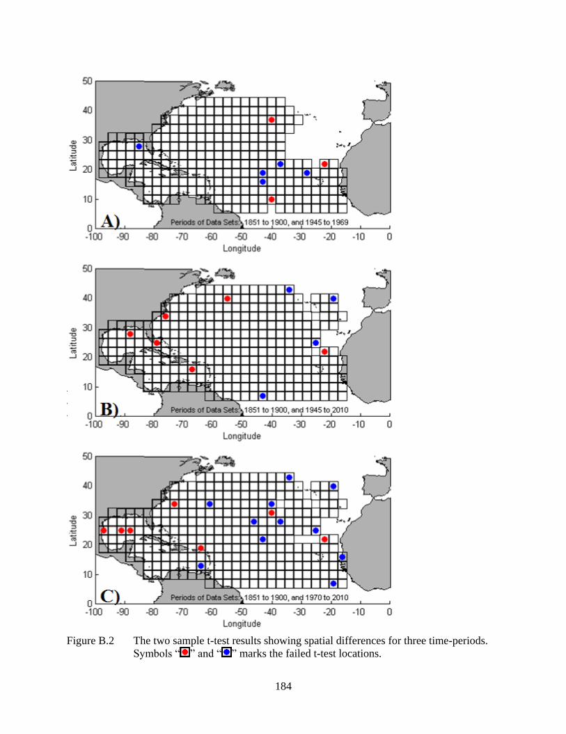
184

Figure B.2 The two sample t-test results showing spatial differences for three time-periods.

Symbols “ ” and “ ” marks the failed t-test locations.

185

In general, longitudinal expected probabilities are show similar trends for each one of the

periods. However, Latitudinal expected probabilities show a change in higher than 30° N

latitudes in the North Atlantic (not including Gulf of Mexico).

Figure B.3 Exceedance probability of track coordinates in the North Atlantic (not including

Gulf of Mexico).

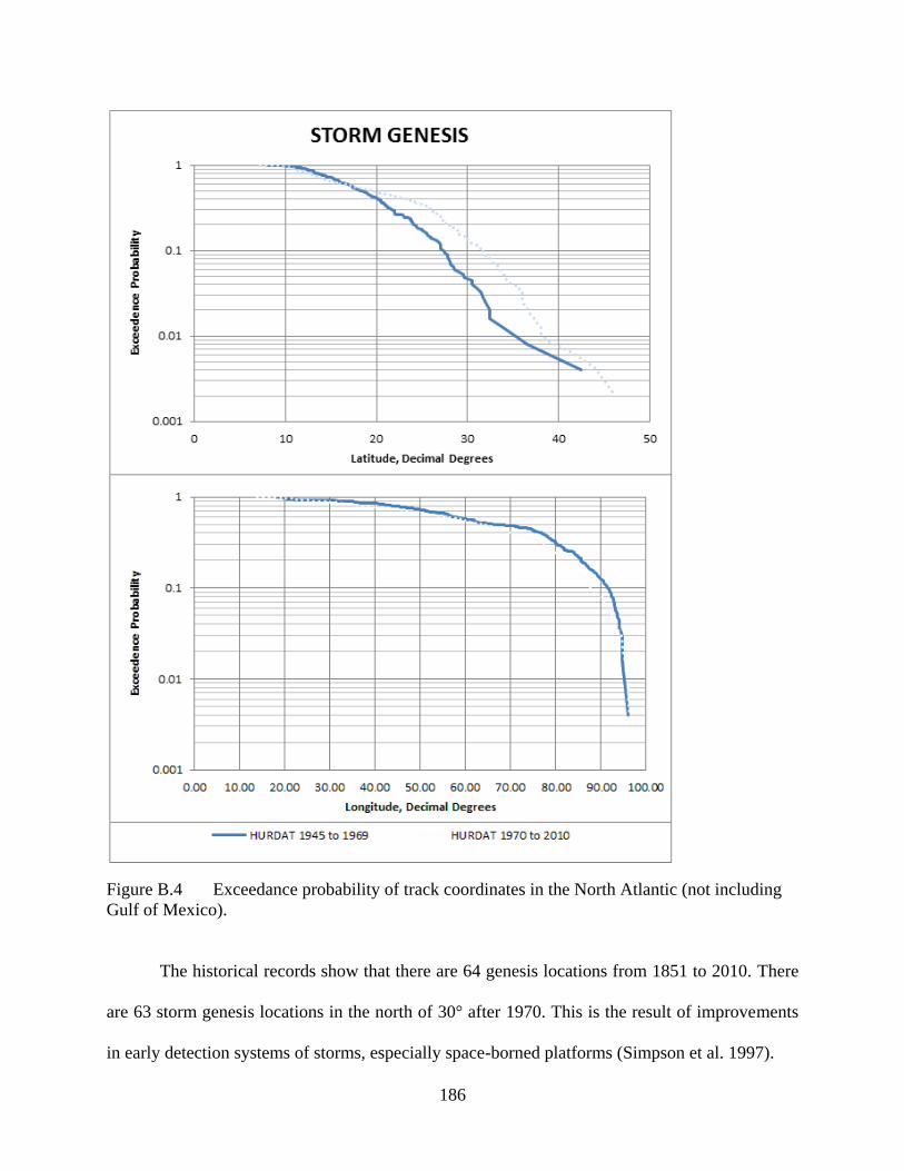
186

Figure B.4 Exceedance probability of track coordinates in the North Atlantic (not including

Gulf of Mexico).

The historical records show that there are 64 genesis locations from 1851 to 2010. There

are 63 storm genesis locations in the north of 30° after 1970. This is the result of improvements

in early detection systems of storms, especially space-borned platforms (Simpson et al. 1997).

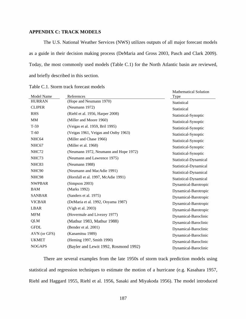
187

APPENDIX C: TRACK MODELS

The U.S. National Weather Services (NWS) utilizes outputs of all major forecast models

as a guide in their decision making process (DeMaria and Gross 2003, Pasch and Clark 2009).

Today, the most commonly used models (Table C.1) for the North Atlantic basin are reviewed,

and briefly described in this section.

Table C.1. Storm track forecast models

Model Name

References

Mathematical Solution

Type

HURRAN (Hope and Neumann 1970) Statistical

CLIPER (Neumann 1972) Statistical

RHS

(Riehl et al. 1956, Harper 2008) Statistical-Synoptic

MM

(Miller and Moore 1960) Statistical-Synoptic

T-59

(Veigas et al. 1959, Bril 1995) Statistical-Synoptic

T-60

(Veigas 1961, Veigas and Ostby 1963) Statistical-Synoptic

NHC64

(Miller and Chase 1966) Statistical-Synoptic

NHC67

(Miller et al. 1968) Statistical-Synoptic

NHC72

(Neumann 1972, Neumann and Hope 1972) Statistical-Synoptic

NHC73

(Neumann and Lawrence 1975) Statistical-Dynamical

NHC83

(Neumann 1988) Statistical-Dynamical

NHC90

(Neumann and MacAdie 1991) Statistical-Dynamical

NHC98

(Horsfall et al. 1997, McAdie 1991) Statistical-Dynamical

NWPBAR

(Simpson 2003) Dynamical-Barotropic

BAM

(Marks 1992) Dynamical-Barotropic

SANBAR

(Sanders et al. 1975) Dynamical-Barotropic

VICBAR

(DeMaria et al. 1992, Ooyama 1987) Dynamical-Barotropic

LBAR

(Vigh et al. 2003) Dynamical-Barotropic

MFM

(Hovermale and Livezey 1977) Dynamical-Baroclinic

QLM

(Mathur 1983, Mathur 1988) Dynamical-Baroclinic

GFDL

(Bender et al. 2001) Dynamical-Baroclinic

AVN (or GFS)

(Kanamitsu 1989) Dynamical-Baroclinic

UKMET

(Heming 1997, Smith 1990) Dynamical-Baroclinic

NOGAPS

(Bayler and Lewit 1992, Rosmond 1992) Dynamical-Baroclinic

There are several examples from the late 1950s of storm track prediction models using

statistical and regression techniques to estimate the motion of a hurricane (e.g. Kasahara 1957,

Riehl and Haggard 1955, Riehl et al. 1956, Sasaki and Miyakoda 1956). The model introduced

188

by Riehl and Haggard (1956) is an example of a technique that uses current synoptic information

to predict the future storm location. In this method, the storm center is displaced with the mean

geostrophic wind. The geostrophic winds are calculated rectangular box computation window

superimposed on the storm location. Empirical models that include large-scale information as

predictors of future location or intensity are referred as “statistical-synoptic models”. In the early

1970s, the HURRAN and CLIPER models (Hope and Neumann 1970, Neumann 1972) were

developed and included parameters related to the hurricane itself (e.g. location, time and storm

strength) for prediction. These types of models are referred to as “statistical models” in Table

3.1.

STATISTICAL MODELS

These models are the simplest complexity models used for tropical cyclone track

forecast. These models utilize historical tropical cyclone track information as predictors of future

location or intensity.

HURRAN (HURRicane ANalog): This forecasting model was developed at the National

Hurricane Center in 1969 and become operational in 1970 (Hope and Neumann 1970,

Neumann and Hope 1972). The HURRAN model is designed to resolve the most likely path

of current storm by utilizing a database of historical storm records from 1886 to 1969. In

later years, the coverage of database extended to include 782 storms from 1886 to 1979.

HURRAN model computes as its output the following storm parameters: storm direction,

wind speed, and storm locations. In the described study, the HURRAN model methodology

is enhanced by including storm intensity related parameters: Holland B, and Rmax.

CLIPER (CLImatology and PERsistence): CLIPER is a statistical track prediction model that

uses regression equations to model the storm path. CLIPER resolves the most likely path

189

using following predictors: previous storm motion, latitude, longitude, and time (Aberson

1998, Neumann and Hope 1972). CLIPER uses least-square fitting of continues polynomial

functions. This models is still in use by NOAA to benchmark other track models (Aberson

and Sampson 2003).

STATISTICAL - SYNOPTIC MODELS

These models are hybrid-statistical models used for tropical cyclone track forecast. The

difference is that these models utilize both historical tropical cyclone track information and

current synoptic data as predictors of future location or intensity.

RSH (Riehl-Haggard-Sanborn): This is regression model which utilizes geostrophic winds as

a predictor (Riehl et al. 1956). In this approach, the movement of storm is computed by the

displacement of the storm center with mean 500 hPa geostrophic winds expected to influence

storm motion during the next 24 hour by using a large rectangular kernel superimposed on

the wind-field of the storm. The RHS model is considered to be an objective track model

(Birchfield 1960).

MM (Miller-More): MM is a statistical regression model which utilizes 700 hPa geostrophic

winds, past storm location, and motion as predictors (Miller and Moore 1960). The

regression equations were derived from data of 18 hurricanes from the North Atlantic Basin

between 1951 and 1956. This model was not used in forecast after the 1962 because of its

poor performance in storm forecast.

T-59 (Traveler's-National Hurricane Research Laboratory 1959): The T-59 is a statistical

model utilizing surface pressure and past storm motion as predictor (Veigas 1961, Veigas et

al. 1959). The sea-level pressure data used in the model are obtained from 5×5 degree grid

points bounded by a domain of 30°N and 60°W in North Atlantic Basin. The regression

190

model was developed using 447 historical storm records. T-59 calculations perform well in

respect to surface pressure values, but it is sensitive to errors in locating to storm center

(Gentry 1964). For example, if the storm slows down quickly, this model tends to the

forecast location of storm with larger errors.

T-60 (Traveler's-National Hurricane Research Laboratory 1960): T-60 is a statistical

regression model which utilizes 500 hPa geostrophic winds, surface pressure, and past storm

motion predictors. This model was developed through cooperation between the National

Hurricane Research Laboratory and Travelers Research Center to improve previous statistical

forecasting models, such as T-59 (Dunn et al. 1968, Veigas 1961, Veigas and Ostby 1963).

NHC64 (or , A64E): This model is a regression model which utilizes 500 and 700 hPa

heights, geostrophic wind, surface pressure, 1000-700 hPa, and 500-700 hPa thickness and

past storm motion as predictor. (Miller and Chase 1966)

NHC67 (or, A67E): This is a regression model that takes CLIPER output, and current and

past (24 h) 1000, 700 and 500 hPa heights as inputs (Miller et al. 1968). NHC67 was an

updated version of the statistical-synoptic NHC64 model (Miller and Chase 1966).

NHC72 (or A72E): The NHC72 model is very similar to NHC67 model in model

implementation. Both models use the same current and past storm information, and take the

same wind heights as inputs. The difference of NHC72 model from NHC67 model is that the

CLIPER output is modified before used in prediction calculation of the NHC72 model

(Aberson 2001, Neumann et al. 1972). This model was operational from 1972 to 1988.

191

STATISTICAL-DYNAMICAL MODELS

Statistical-dynamical forecast models are hybrid models in utilization of storm predictors. These

models solve both dynamical and statistical procedures by utilizing historical and current

atmospheric predictors for predicting the future location of a storm.

NHC73 (or, A73E): This model is a regression model and was the first statistical-dynamical

model implemented by NHC. The algorithm of NHC73 model is given in Figure 3.1

(Neumann and Lawrence 1975). The model uses the outputs of three forecast models as

input.1) output from CLIPER model which uses storm's current and past motion, the storm's

current location, current date and maximum wind as input; 2) output of steering forecast

which includes 1000, 700 and 500 hPa as inputs into gridded analysis; and 3) output of the

National Meteorological Center's (NMC) primitive equation model (Shuman and Hovermale

1968) which uses 24-, 36- and 48-h geo-potential heights as inputs. In addition, the model

uses a number of overlapping layers of dependent data, which is divided into 52 sections in

the North Atlantic Basin.

Figure C.1 The algorithm of NHC73 (Neumann and Lawrence 1975)

192

NHC83: NHC83 (Neumann 1988) is a regression model consisting of five sub-systems

which are referred to as Models 1 through Models 5. Models 1, 2, and 3 uses outputs of

CLIPER, observed 1000 -100 hPa geopotential heights, and numerically forecast mean

geopotential heights as predictors. The Model 4's output is given as inputs to Models 1 and 2.

The Model 5 produces an output performing a least-square fitting of Models 1 - 3. The North

Atlantic Domain is divided into two parts at 25°N (for each one of the regression models).

The algorithm diagram of NHC83 is given in Figure 3.2 (Neumann 1988). The historical data

set contains the track information from 1962 to 1981.

Figure C.2 The NHC83 algorithm (Neumann 1988)

NHC90 and NHC 98: NHC90 (Neumann and MacAdie 1991) model algorithm is the same as

the NHC83 model algorithm. The only difference between these models is the data sample

that is used to drive the systems. NHC90 uses the data from 1975 to 1988 (McAdie 1991).

The NHC98 model is the last one of the statistical-dynamic track forecast models developed

by Nation Weather Services (NWS). The NHC98 contains methods to remove tropical

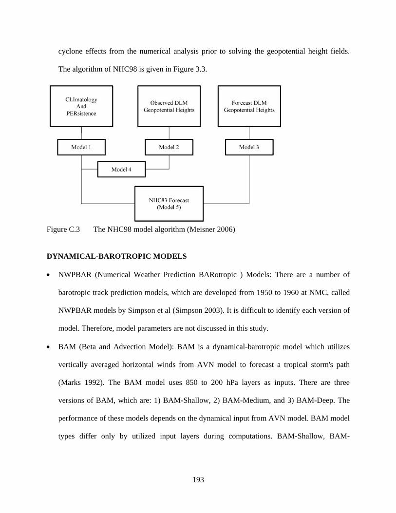
193

cyclone effects from the numerical analysis prior to solving the geopotential height fields.

The algorithm of NHC98 is given in Figure 3.3.

Figure C.3 The NHC98 model algorithm (Meisner 2006)

DYNAMICAL-BAROTROPIC MODELS

NWPBAR (Numerical Weather Prediction BARotropic ) Models: There are a number of

barotropic track prediction models, which are developed from 1950 to 1960 at NMC, called

NWPBAR models by Simpson et al (Simpson 2003). It is difficult to identify each version of

model. Therefore, model parameters are not discussed in this study.

BAM (Beta and Advection Model): BAM is a dynamical-barotropic model which utilizes

vertically averaged horizontal winds from AVN model to forecast a tropical storm's path

(Marks 1992). The BAM model uses 850 to 200 hPa layers as inputs. There are three

versions of BAM, which are: 1) BAM-Shallow, 2) BAM-Medium, and 3) BAM-Deep. The

performance of these models depends on the dynamical input from AVN model. BAM model

types differ only by utilized input layers during computations. BAM-Shallow, BAM-

194

Medium, and BAM-Deep models use 850-700 hPa, 850-400 hPa, and 850-200 hPa layers,

respectively.

SANBAR (SANders BARatropic) Model: Sanders (Sanders et al. 1975) implemented a

barotropic track forecast model for the North Atlantic Basin that is known as the SANders

BARotropic model. This model implements a finite difference approach to solve the

barotropic vorticity equation. The model uses averaged 1000 - 100 hPa wind fields as input

over the model domain (Burpee 2008). There are a number of versions of the SANBAR

model with varying grid resolution from 0.75° to 1.5° for each cell.

VICBAR (VIC Ooyama BARotropic) Model: VICBAR is a dynamical-barotropic track

forecast model which perceives the atmospheres as a single layer of fluid (DeMaria et al.

1992). The model equations are solved in a number of nested domains based on the spectral

finite-element representation method developed by Ooyama (Ooyama 1987). In summary,

these models consist of two parts: an analysis scheme and a barotropic prediction module.

This model utilizes four meshes with varying area coverage and cell sizes. VICBAR

averaged vertical layer wind and height layers are determined by analysis of 850, 700, 500,

400, 200 and 200 hPa wind fields (Aberson and DeMaria 1994).

LBAR (Limited area sine-transform BARotropic) Model: LBAR is a dynamical-barotropic

track prediction model (Vigh et al. 2003). This model is a simplified version of the VICBAR

model. (Simpson 2003)LBAR solves the shallow-water wave equations using some averaged

850 - 200 hPa winds and heights layers as inputs from AVN model output. The model

equations are solved using spectral sine transform approach, hence the name comes.

195

DYNAMICAL-BAROCLINIC MODELS

MFM (Moveable Fine Mesh) Model: The MFM (Hovermale and Livezey 1977) is a

dynamical-baroclinic forecast model which utilizes primitive equations to calculate forecast

parameters. The model contained 10 vertical levels over a regular grid with 60 km cell

resolution covering a 3000×3000 km area over the North Atlantic Domain. The storm is

centered on the moving horizontal domain and the boundary conditions were obtained from

the Limited-area Fine Mash (LFM) model prior to 1984 (DeMaria et al. 1990). The model

was run from an initialized state by a version of the model with no environmental flow before

the 1983. Beginning 1983, the storm wind field was initialized from a three-dimensional

model that calculated the Coriolis effect by using storm latitude (Simpson 2003).

QLM (Quasi-Lagrangian Model): The QLM (Mathur 1983, Mathur 1988) is a dynamical-

baroclinic forecast model which is very similar to MFM. The QLM differs from MFM in the

following areas: increased horizontal resolution (40 km by 40 km finer grid mesh), larger

domain (4400 km by 4400 km), increased vertical resolution (18 levels) and the model

domain does not move to place the storm into the center of the model domain. The name of

the model comes from the mathematical method used for solving the equations (Simpson

2003).

GFDL (Geophysical Fluids Dynamics Laboratory) Model: The GFDL is a limited-area,

nested moveable mesh dynamical-barotropic track forecast model which was developed by

Geophysical Fluids Dynamics Laboratory at Princeton University (Bender et al. 2001). Since

the 1990s, GFDL model has been developed to increase accuracy and grid resolution (Bender

et al. 2001, Kurihara et al. 1995). Currently, the model has 42 vertical layers, and three

196

nested grids, as illustrated in Figure 3.4. Table 3.4 lists the latest grid and domain

information for GFDL versions (Pasch and Clark 2009).

AVN: AVN model is a baroclinic-dynamical track forecast component of Global Forecast

System (GFS). AVN uses “synthetic” observations in Medium-Range-Forecast model of

NCEP for data assimilation. The first operational version of the model utilizes 28 vertical

layers over T126 grid (Kanamitsu 1989). The current grid has a horizontal resolution of 76

km (T170 grid).

Table C.2 Existing GFDL model domain and grid information

Model Name

Global Model Boundary

Conditions

Horizontal Grid Spacing

Vertical

Levels

GFDL

AVN (or, GFS)

75° x 75° Outer grid ~30 km

11° x 11° Middle grid ~10 km

5° x 5° Inner grid ~5km

42

GFDN

NOGAPS

75° x 75° Outer grid ~30 km

11° x 11° Middle grid ~10 km

5° x 5° Inner grid ~5km

42

Figure C.4 The GFDL model domain extent and grids (Source: Web1)

UKMET: This model is developed by United Kingdom METeorological (UKMET) Office

(Skinner and Hart 1996, Skinner and Hart 1997). The UKMET model is a global model with

approximately 40 km grid cell size. This model has 50 vertical layers. The model was

197

modified twice to solve physical parameters with different type of equations in 2002, and in

2005 (Pasch and Clark 2009, Untch 2009). The UKMET model is very accurate in predicting

the storm path. Although, the accuracy in intensity forecast of the model is limited.

NOGAPS (Navy Operational Global Atmospheric Prediction System): The NOGAPS model

is a dynamical-baroclinic storm track forecast model which utilizes following approaches to

solve primitive equations: second-order finite difference in the vertical, and central time

differencing with Robert semi-implicit corrections (Bender et al. 2001). Currently, the model

uses T239 grid, has approximately 56 km resolution on horizontal spacing, for spectral

truncation (Liu et al. 2010, Pasch and Clark 2009).

STORM INTENSITY FORECAST MODELS

These models are used to forecast future intensity of a tropical cyclone. These models are

usually integrated with tropical cyclone track models.

Statistical Hurricane Intensity Prediction Scheme (SHIPS): SHIPS is a statistical-synoptic

model utilizes climatology and persistence, atmospheric environmental parameters (e.g.

vertical winds between the 850 - 200 hPa), the difference between the current and past

intensity, and oceanic input (e.g. sea surface temperature--SST) as predictor parameters to

forecast intensity changes (Demaria and Kaplan 1994). The multiple regression equations for

this approach are developed using storm data from 1982 through present (Demaria and

Kaplan 1994, DeMaria et al. 2005a, DeMaria et al. 2005b). Each one of the regression

equations are updated by including previous season's storm data. The statistical-synoptic

version of the SHIPS used from 1991 to 1996 by NWS. The SHIPS model was updated to

statiscal-dynamical prediction model in 1997 (DeMaria et al. 2005b). Another modification

took place with inclusion of inland storm decay module in 2000.

198

SHIFOR (Statistical Hurricane Intensity FORecast) Model: SHIFOR is a statistical intensity

prediction model that uses climatologically and persistence parameters. The forecast

parameters are day, current storm intensity, change in intensity during previous 12 hour,

latitude and longitude of storm location, and storm motion vectors on x and y coordinates

(Jarvinen and Neumann 1979). The water bound storms data from 1900 to 1972 were used in

developing the model equations. The regression equations of SHIFOR5 version developed by

utilizing storm data between the years 1967 and 1999 (Knaff et al. 2003).

GFDL Model: GFDL model has modules that are used for intensity forecast. GFDL model is

described in the track forecast models section (Bender et al. 2001, LANL 2010).

ENSEMBLE FORECAST MODELS

These models are, also, called consensus models. These models attain a tropical cyclone

track by combining multiple track forecasts. Table C.3 lists ensemble models used in forecast.

Table C.3 Ensemble models used for tropical cyclone forecast in the North Atlantic Basin

Model Name

Ensemble Type

Model Type

Combined Forecast Models

GUNA

Average

Track Model

Consensus of AVNI, GFDI, EGRI and NGPI Models

TCON/TCOE

Average

Track Model

Consensus of AVNI, EGRI, NGPI, GHMI, and HWFI Models

TCOA

Average

Track Model

Consensus of AVNI, EGRI, GHMI, and HWFI Models

TVCN

Bias-Corrected

Track Model

Consensus of AVNI, EGRI, EMXI, NGPI, GHMI, HWFI Models

TVCE

Bias-Corrected

Track Model

Consensus of AVNI, EGRI, EMXI, NGPI, GHMI, GFNI, HWFI Models

TVCA

Bias-Corrected

Track Model

Consensus of AVNI, EGRI, EMXI, GHMI, GFNI, HWFI Models

RYOC/MYOC

Average

Track Model

Forecaster-Generated Consensus Guidance

CGUN

Bias-Corrected

Track Model

GUNA Forecast

TCCN

Bias-Corrected

Track Model

TCON Forecast

TVCC

Bias-Corrected

Track Model

TVCN Forecast

IVCN

Bias-Corrected

Intensity

Consensus of DSHP, LGEM, HWFI, GHMI, and GFNI Models

SPC3

Average

Intensity

Consensus of AVNI, GHMI, HWFI models

199

APPENDIX D: HURRAN MODEL

This section provides information about the HURRAN model data input and output

formats. Also, the model algorithm is provided.

Figure D.1 Punch card for tropical cyclone Anita, 1977 (Jarvinen et al. 1984).

HURDAT FILE FORMAT DESCRIPTION

(Source: NOAA Technical Memorandum NWS NHC 22 (1984))

HEADER:

92620 08/16/1992 M=13 2 SNBR= 899 ANDREW XING=1 SSS=4

Card# MM/DD/Year Days S# Total#... Name........US Hit.Hi U.S. category

DAILY DATA:

92580 04/22S2450610 30 1003S2490615 45 1002S2520620 45 1002S2550624 45 1003*

Card#

MM/DD&LatLongWindPress&LatLongWindPress&LatLongWindPress&LatLongWindPress

TRAILER:

92760 HRCFL4BFL3 LA3

Card# TpHit.Hit.Hit.

200

HEADER:

Card# = Sequential card number starting at 00005 in 1851

MM/DD/Year = Month, Day, and Year of storm

Days = Number of days in which positions are available (note that this also means number of

lines to follow of Daily Data and then the one line of the Trailer)

S# = Storm number for that particular year (including subtropical storms)

Total# = Storm number since the beginning of the record (since 1851)

Name = Storms only given official names since 1950

U.S. Hit =

'1' = Made landfall (i.e. the center of the cyclone crossed the coast) on the continental United

States as a tropical storm or hurricane,

'0' = did not make a U.S. landfall

Hi U.S. category =

'0' = Used to indicate U.S. tropical storm landfall, but this has not been utilized in recent years

'1' to '5' = Highest Saffir-Simpson Hurricane Scale impact in the United States based upon

extimated maximum sustained surface winds produced at the coast. See scale below.

DAILY DATA:

Card# = As above.

MM/DD = Month and Day

Positions and intensities are at 00Z, 06Z, 12Z, 18Z

& =

'*' (tropical cyclone stage),

'S' (Subtropical stage)

'E' (extratropical stage)

'W' (wave stage - rarely used)

'L' (remanent Low stage - rarely used)

Lat = Latitude of storm: 24.5N

Long = Longitude of storm: 61.0W

Wind = Maximum sustained (1 minute) surface (10m) windspeed in knots (these are to the

nearest 10 knots for 1851 to 1885 and to the nearest 5 kt for 1886 onward).

Press = Central surface pressure of storm in mb (if available). Since 1979, central pressures are

given everytime even if a satellite estimation is needed.

TRAILER:

Card# = As above.

Tp = Maximum intensity of storm

'HR' = hurricane

'TS' = tropical storm

'SS' = subtropical storm

Hit = The impact of the hurricane on individual U.S. states ('LA' = Louisiana, etc.) based upon

the Saffir-Simpson Scale category (through the estimate of the maximum sustained surface

winds for each state). See scale below. Occasionally, a hurricane will cause a hurricane impact

(estimated maximum sustained surface winds) in an inland state. To differentiate these cases

versus coastal hurricane impacts, these inland hurricane strikes are denoted with an “I” prefix

before the state abbreviation. States that have been so impacted at least once during this period

201

include Alabama (IAL), Georgia (IGA), North Carolina (INC), Virginia (IVA), and

Pennsylvania (IPA). The Florida peninsula, by the nature of its relatively landmass, is all

considered as coastal in this database.

Note that Florida and Texas are split into smaller regions:

'AFL' = Northwest Florida

'BFL' = Southwest Florida

'CFL' = Southeast Florida

'DFL' = Northeast Florida

'ATX' = South Texas

'BTX' = Central Texas

'CTX' = North Texas

AN EASIER TO READ VERSION OF HURDAT

Storm ETHEL is number 6 of the year 1960

************************************************ Month Day Hour Lat. Long. Dir. ----Speed----- -----Wind------ Pressure ------------Type-----------

September 14 12 UTC 23.9N 90.6W -- deg -- mph -- kph 45 mph 75 kph -- mb Tropical Storm

September 14 18 UTC 25.6N 89.7W 25 deg 20 mph 33 kph 85 mph 140 kph -- mb Hurricane - Category 1

September 15 0 UTC 27.0N 89.1W 20 deg 16 mph 25 kph 125 mph 205 kph 981 mb Major Hurricane - Category 3

September 15 6 UTC 28.1N 88.9W 10 deg 12 mph 20 kph 160 mph 260 kph -- mb Major Hurricane - Category 5

September 15 12 UTC 29.1N 88.9W 0 deg 11 mph 18 kph 90 mph 150 kph -- mb Hurricane - Category 1

September 15 18 UTC 29.9N 89.0W 355 deg 9 mph 14 kph 70 mph 110 kph -- mb Tropical Storm




September 16 18 UTC 32.9N 88.5W 20 deg 10 mph 16 kph 35 mph 55 kph -- mb Tropical Depression





Table D.1 Saffir-Simpson Scale

Maximum sustained wind speed

Category mph m/s kts

1 74-95 33-42 64-82

2 96-110 43-49 83-95

3 111-130 50-58 96-113

4 131-155 59-69 114-135

5 156+ 70+ 136+

202

Figure D.2 HURRAN model algorithm (Hope and Neumann 1970)

Compute speed and

direction bias

Compute 3-hrly

storm positions Count cases

Scan array of 3-hrly

storm positions

Compute hourly

forecast positions

Select position

closest to center of

acceptance circle

Rotate initial portion

of past storm track

Compute 12-hrly

speed and direction

of movement

Adjust speed on

initial portion of past

storm track

Store 12, 24, 36, 48,

and 72 hour adjusted

storm positions

Store acceptable

positions

Translate past storm

positions

Fit 12, 24, 36, 48 and

72 hr arrays to

bivariate normal

distribution

Read in

variables

Read in

one storm

Write

results

Plot storm

tracks

Stop

Start

Yes No

Yes

No Yes

No

Yes

Yes

Yes

Yes

No

No

No

No Is date within

limits?

Is speed within

limits?

Is direction

acceptable?

Is position with-

in circle?

Is scanning

complete?

At least 5

cases?

End of data

file?

Write calcomp tape

for offline plot

203

APPENDIX E: SURGE MODELS

This section provides literature on storm surge. Also, the Ocean Circulations Models are

reviewed.

EXISTING DETERMINISTIC STORM SURGE MODELS

Storm surge from hurricanes and tropical cyclones is simply water pushed by winds

toward the shore. The level of surge in a region is largely determined by three factors: 1) the

slope of the continental shelf, 2) the speed of the driving winds, and 3) astronomical tide levels

(Pugh 1987, Pugh and Vassie 1979). The generalized storm surge elevation is defined in

Equation 6.1 (Pugh 1987). Note that the definition of storm surge does not include superimposed

waves. The simplified storm surge from tropical cyclones is also illustrated in Figure E.1 (Harper

2001, Harper 2008). The following sections discuss existing storm surge model types, as well as

providing information on historical models.

( ) ( ) ( ) ( ) (6.1)

where

S(t) = meteorological surge at time t

X(t)= sea level measurement at time t

Z0(t)= mean sea level at time t

T(t)= tidal component at time t

Astronomical tide elevations are deterministic in coastal regions, therefore; they are not

included as an unknown in our computations. Pugh et al. (1979, 1980) discuss tide and surge

probability for extreme sea level estimations. They computed extreme high water probabilities

by utilizing an approach that combines of Joint Probability Method (JPM) and frequency

distribution of tide and storm surge components with shorter time-periods. The surge level

calculations for southwestern coastal Louisiana incorporated modified version of JPM for

204

tropical cyclone track selection (Toro et al. 2007, Toro et al. 2010b). Similar to above mentioned

studies, in this study, the probability distributions are used to define the key storm surge

parameters.

Figure E.1 Simplified storm surge illustration

The storm surge elevation composed of various components. For example, wave setup

and surge are two of those components (Figure E.1). The hydrodynamics of storm tide formation

in coastal zones are well-known due to the large number of studies (Ackers and Ruxton 1975,

Führböter 1979, Jarvinen and Gebert 1987, Jelesnianski 1972, Pugh 1987). However, accuracy

of the storm surge prediction models largely depends on the precision of meteorological input

and completeness of historical surge data for tropical cyclones (Harper 2001). For example,

during Hurricane Katrina (2005), a number of key tide stations were damaged and stopped

recording storm surge elevations. As a result, there is a lack of complete surge elevation records

for strong tropical cyclones. This lack of completeness presents a problem by influencing the

reliability of storm surge elevation estimation.

205

OCEAN CIRCULATION MODEL CLASSIFICATION

In this section, historical development of Ocean Circulation Models (OCMs) is reviewed.

This review helps to understand the capabilities of existing OCMs. Until the 1990s, regional and

global OCMs did not have sophisticated parallel computing algorithms or grid-computing

capabilities. Computational power advances in newer OCMs corresponded with the development

of more powerful computer hardware and very efficient computer algorithms for

computationally demanding and complex problems. Despite the advances in computational fluid

dynamics, OCMs use a single family of models that was initially developed by Bryan and Cox in

the 1960s (LANL 2010, Simpson 2003, Willoughby et al. 2007). The genealogy of the

Geophysical Fluid Dynamics Laboratory (GFDL) model is shown going back to the Modular

Ocean Model (MOM) in Figure E.2.

The literature review will focus on model extents, which are Basin and Global Models in

the section 4.2. After that, the mathematical solution based on the literature review is given in the

section 4.5.

OCEAN CIRCULATION MODELS CLASSIFICATION BY MODEL EXTENT

OCMs are generally classified by two criteria: domain extent (e.g. basin or global) and

mathematical solution approach of modeled equations (e.g. finite element method, finite

difference method). Basin models cover a smaller geographical area on the earth surface, and

may range in size range from a bay to an ocean. The basin model extent can be as small as an

inlet, or as large as an ocean. For example, Sea, Lake and Overland Surges from Hurricanes

(SLOSH) model is a small-extent basin model (Jarvinen and Gebert 1987, Jelesnianski 1972).

These models are implemented in different regions of the world such as the Pacific, the North

Atlantic, the North Sea and the Mediterranean. The other basin model, the ADvanced

206

CIRCulation (ADCIRC) model, has been implemented over a number of different domain

extents ranging from the Mediterranean Sea basin to the North Atlantic Ocean basin (Luettich et

al. 1992).

On the other hand, the computational extent of global models (e.g GFDL model) covers

entire earth surface. One of the most well-known global ocean circulation models is Geophysical

Fluid Dynamics Laboratory (GFDL) model. The atmospheric component of GFDL model is

partly discussed in Chapter 2. The GFDL model is composed of a number of model components,

such as atmospheric, or ocean component. The genealogy of the Geophysical Fluid Dynamics

Laboratory (GFDL) model is shown going back to MOM in Figure E.2 and Figure E.3 (Bender

et al. 2001, LANL 2010, Pasch and Clark 2009). See Table E.1 for the names, types, authors and

years for these models.

Figure E.2 GFDL model genealogy (LANL 2010)

207

The Ocean and Climate Group at GFDL continued their efforts for improving the GFDL

model. As a result, the expansion of the family tree by adding the developed GFDL models since

late 1990s is illustrated in Figure E.3. The latest version of the MOM, which is released in 2009,

is called MOM4.1 (Griffies et al. 2009). The MOM4.1 incorporated additional functionality of

vertical coordinates and non-Boussinesq effects. Generalized Ocean Layer Dynamics (GOLD)

model (Lin 2004) is a descendent of Hallberg Isopycnal Model (HIM) (Hallberg 1995). MOM4.1

and GOLD models are going to be blended into as of yet the unnamed next generation model.

Figure E.3 GFDL model genealogy update after (LANL 2010)

OCEAN CIRCULATION MODEL CLASSIFICATION BY MATHEMATICAL MODEL

OCMs continue to rely on a single family of mathematical methods that solve partial

differential equations in a variety of methods. There are four major approaches to solving partial

differential equations: (1) spectral or spectral transform, (2) finite difference, (3) finite element,

and (4) finite volume. The spectral techniques are very difficult to implement in OCMs because

of complex ocean and model boundaries. Therefore, spectral or spectral transform approaches

have not been widely implemented in Ocean Circulation Models. The Finite Difference Method

208

(FDM) is the first method used in the OCMs. This method was commonly used due to its

simplicity. Nevertheless, FDM lost its popularity due to the round-off and truncation errors in

OCMs. However, the Finite Element Method (FEM) simplifies such problems because of its

flexibility in representing the coastal features on a Triangulated Irregular Network (TIN) mesh to

any resolution. Therefore, the FEM is the most commonly implemented method for solving

partial differential equations in OCMs. The Finite Volume Method (FVM) offers convergence,

accuracy, and stability for heterogeneous grids as each grid cell can be assigned different

material parameters, such as marsh. In recent years, researchers have implemented FVM in their

ocean circulation models. The major mathematical foundations for the above-mentioned

approaches for solving partial differential equations are shown in model type column of Table

4.1.

Spectral Method (SM): SM techniques implement a Fourier Series to convert partial

differential equation to get a system of ordinary differential equations. The spectral method

global approach that approximates the solution as a linear combination of continuous

functions. The spectral method usually uses a Gaussian Grid, with large grid cells, generally

ranging from 1 to 5 degrees.

Finite Difference Method (FDM): FDM is a group of techniques to solve some types of

partial differential equations. This method is the easiest method to implement, and

approximates solutions as a linear combination of piecewise functions, which is a local

approach to the solution. The Finite Difference Method uses regular grids (e.g. latitude and

longitude). The grid resolution varies depending on the domain.

Finite Element Method (FEM): FEM is an approach for solving partial differential equations

using discretization. The discretization is done locally over small regions (the finite

209

elements). The biggest advantage of this method is FEM’s flexibility to model complex

surfaces better than other methods. The disadvantage is that it is difficult to implement. The

method is capable of using a variable mesh, resulting in a flexible grid resolution.

Finite Volume Method (FVM): FVM is a numerical method for solving partial differential

equations. This method calculates the values of the conserved variables averaged across a

volume. FVM does not require a structured mesh.

Table E.1 Ocean circulation models

Model Name Model Type Author and Year

ACADIA Finite Element Gentleman (1998)

Advanced Circulation Model (ADCIRC) Finite Element Luettich (1992)

BOM (Bergen Ocean Model) Finite Element Berntsen et al. (1996)

FUNDY Finite Element Lynch and Werner (1987, 1991)

QUODDY Finite Difference Lynch et al. (1995)

Hallberg Isopycnal Model (HIM) Finite Element Hallberg, R. (1995)

Hamburg Ocean Primitive Equation

(HOPE)

Finite Difference

Jörg-Olaf Wolff (1997)

Miami Isopycnic Coordinate Ocean Model

(MICOM)

Finite Difference

Bleck et al. (1995), (1992),

Sawdey et al. (1997)

The MIT General Circulation Model

(MITgcm)

Finite Volume

Marshall (1995), Marshall et al.

(1997)

Navy Layered Ocean Model (NLOM) Finite Element Hurlburt and Thompson (1980)

The Modular Ocean Model (MOM) --GFDL Finite Difference Bryan, K. and M. D. Cox (1972)

The Princeton Ocean Model directory

(POM)

Finite Difference

Blumberg and Mellor (1987)

Parallel Oregon State University Model

(POSUM)

Finite Difference

Higdon and de Szoeke (1997)

S-Coordinates Rutgers University Model

(SCRUM)

Finite Difference

Song and Haidvogel (1994)

The Southampton - East Anglia (SEA)

model

Finite Difference

Beare and Stevens (1997)

Harvard Ocean Prediction System ( HOPS) Finite Element Robinson (1996, 1996)

Parallel Ocean Program(POP) Finite Element Smith et al. (1992)

The NCAR Community Ocean Model

(NCOM)(NCAR)

Finite Element

Gent (2011, 1998), Holland et al.

(1998),

The Regional Ocean Modeling System

(ROMS)

Finite Element

Shchepetkin (1998, 2003, 2005),

Marchesiello (2001, 2003)

The Spectral finite Element Code (SEOM) Spectral Transform Patera (1984)

Spectral Transform Shallow Water Model

(STSWM)

Spectral Transform

Hack and Jakob (1992)

Finite Volume Coastal Ocean Model

(FVCOM)

Finite Volume

Chen et al. (2003))

Terrain-following Ocean Modeling System

(TOMS)

Hybrid

Ezer and Mellor (2000, 2004),

Chassignet et al. (2000), Haidvogel

et al. (2000)

210

STATISTICAL STORM SURGE MODELING

Joint Probability Method (JPM) Ensemble Approach

In recent years, ensemble approaches to stochastic modeling have gained popularity

(Nong et al. 2010, Smith et al. 2009). Ensemble approaches rely on simulation of a number of

parallel hurricane tracks with the purpose of generating a maximum storm surge elevation for

each category of tropical cyclones over a small domain. The exceedence probability of a storm

surge event is then calculated based on the simulated and historical records. The JPM is an

ensemble methodology that integrates both influencing storm parameters and their associated

probabilities into surge calculations (Niedoroda et al. 2010, Pugh and Vassie 1979, Tawn 1988,

Tawn 1989). In the following sections, a possible implementation of JPM for storm surge

modeling will be discussed.

Joint probability law governs the behavior of two or more random variables when they

are considered at the same time. Random variables are either discrete or continuous (Hawkes

2005). Storm parameters such as wind speed, storm direction, or storm radius are suitable factors

for joint probability analysis of storm surge levels. The joint probability approach calculates a

probability surface for a storm event by considering all possible variations of factors, where each

factor is considered as a random variable. The result is the annual exceedence probability for any

elevation of storm surge (Toro et al. 2007). The Joint Probability Mass Function (PMF) is used if

the random variables are discrete (For PMF, summation is unity). Otherwise, the Joint

Probability Density Function (PDF) is used in calculating the probability. Since a PDF gives the

volume under the probability function, JPM is a multi-dimensional integral that requires

intensive computational time (Ho and Myers 1975, Muradoglu et al. 2003, Toro et al. 2007, Toro

et al. 2010a).

211

The Joint Probability Method was developed for surge inundation probabilities from

hurricanes in the 1970s (Ho and Myers 1975, Myers 1975). Initial implementations of the

methodology showed improvements over other models in terms of storm surge estimation

accuracy. For example, JPM has been implemented for predicting extreme values of sea levels

from short-term observations (Pugh and Vassie 1979, Pugh and Vassie 1980, Tawn 1988, Tawn

1992). The shortcomings of JPM in estimating extreme surge levels estimations are addressed by

the Revised Joint Probability Method (RJPM) (Tawn 1989). In later years, efforts to improve

calculation accuracy by integration of high resolution topographic and wave related data led to

more accurate algorithms. The downside to this is that the mathematical formulas became

increasingly computationally intensive, leading to significant time required to run the full model

ensemble. As a result, JPM-Optimal Sampling (JPM-OS) methods resulted from attempts to

reduce computational requirements (Niedoroda et al. 2007, Toro et al. 2007, Toro et al. 2010a,

Toro et al. 2009).

Storm surge modeling methods are reviewed to understand the state of the art in storm

surge estimation approaches. Advantages and disadvantages of JPM are investigated to identify

the most suitable JMP to use in the study. In the next section, a possible JPM implementation is

explained.

212

APPENDIX F: NEURAL NETWORK

This section provides a brief literature review of neural network modeling approach.

Also, this section presents both statistical and modeling related terminology.

NEURAL NETWORK APPROACH

Neural Networks (NNs) are, in statistical terms, a group of flexible nonlinear regressions

models used for discrimination, reduction, and estimation of data in nonlinear systems

(Kretzman 1994, Sarle 1994). NNs consist of simple linear or nonlinear computing elements,

called “neurons”. In NNs, neurons are interconnected in various fashions ranging from simple to

complex. Neurons are often organized into layers. These three building blocks (neurons,

interconnects, layers) create a neural network. Figure F.4 illustrates the common structures of

simple, complex and multilayer neural networks. In this figure, the equivalent computer science

and statistical terminologies are given above and below the diagram symbols, respectively. For

example, “X” is defined as “input” in computer science terminology and as “independent

variable” in statistical terminology. In NNs, the aim is to determine the relationships between

input and output such that the differences between the output values and target values are

minimized.

Neural networks are utilized in three ways. The first way is representations of biological

nervous systems which is not related to NN utilization in this study. For example, McCullah and

Pitts (1943) illustrated a NN mimic a biological neuron. The second way is used for controlling

and processing the data for real-time adaptive systems. For example, Huang (2007) is

implemented a real-time water level prediction model along Florida coast. Finally, NNs are used

for data processing for analysis methodologies. Tan et al. (2006) utilized NN for cluster

analysis. The second and third utilization ways of NNs are related to this study.

213

In this study, henceforth, the neural networks are referenced with adjective “artificial” to

distinguish the utilization for data analysis. An artificial neural network (ANN) is one of the

methods used in computational intelligence models. The ANN, commonly, is used in developing

data-driven models. In this study, the ANN is used to create the proposed predictive storm surge

methodology. ANN is desirable for usage in soft computing due to tolerance for imprecision and

uncertainty in data (Haykin and Haykin 2009). In addition, ANNs are common in data mining

applications for preparation, reduction and finding dependency rules from data.

Figure F.1 Neural network building blocks and network types (Sarle 1994, pg. 2-5)

The mathematical model for an artificial neuron (an) is modeled after biological neurons

(McCulloch and Pitts 1943). Since 1943, many different models are developed as anns. The

214

differences of anns are in utilized activation function, network topology and learning algorithm.

Rumelhart et al. (1986) proposed the “multi-layer perceptron” (or multi-layer neural network)

and illustrated the suitability of anns for parallel distributed processing. Since late 1986s, anns

have been implemented for various problems in many fields (Tissot et al. 2001, Tissot et al.

2004). For example, the time series related prediction problems are solved for hydrological

applications (e.g. Huang et al. 2007). In this study, anns implementations for tropical storm surge

level estimation is the primary focus.

215

APPENDIX G: COMPUTATION MATRIX

The JPEG file format is a lossy compression method. The quality of a JPEG file changes

with every file write operation due to its compression algorithm. Another problem with images

files is the dithering, means of reducing the color range of images. The dithering reduces the

overall sharpness of image and introduces a grainy pattern into the image. There is a need for

eliminating the effects of these two changes from surge estimation calculations. Therefore, the

storm surge elevations from the images are converted to a matrix structure that stores floating-

point numbers. For the purposes of this dissertation, the matrix structure will be referred as The

computation matrix.

The computation matrix designed based on the image dimensions and image color value

range (color ramp). The dimensions of the original JPEG image files are 500 pixels wide and 285

pixels height. As a result, the computation matrix dimensions are 500 x 285 cells. The image

color ramps are commonly used for mapping colors onto a range of scalar values. The original

NFIS surge files utilize “hot-to-cold” color ramp for visualization of surge elevations. In this

color ram, blue color is chosen for low values, and green color for middle and red color for high

values. Also, there’re other color for indicating physical and imaginary map features, such as

black color for parish boundaries, and dark brown color for roads. These colors are eliminated

from color ramp conversion process. The surge elevation color ramp is converted by using a 5x5

moving window. The developed color ramp conversion program is listed in this section.

The computation matrixes are created for 192 simulated storm surge simulations. These

results are stored in the geo-database. Also, computation matrixes are utilized for the training

artificial neural network.

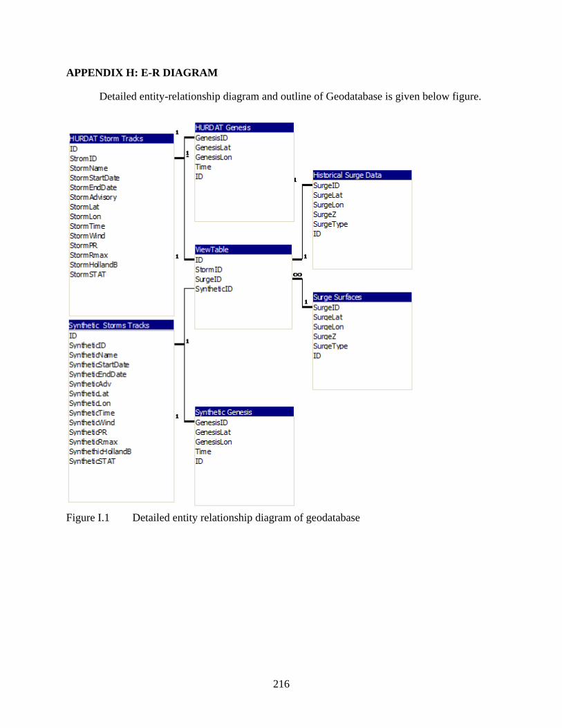
216

APPENDIX H: E-R DIAGRAM

Detailed entity-relationship diagram and outline of Geodatabase is given below figure.

Figure I.1 Detailed entity relationship diagram of geodatabase

217

VITA

Sait A. Binselam was born on June 14, 1970, in Corum, Turkey. He finished his

undergraduate studies at Gazi University, Ankara, Turkey, May 1992. Upon graduation, he

worked as a teacher at a high school for one year. Sait began his graduate study at Louisiana

State University in 1996. He earned his first master of science degree in systems science from

Louisiana State University in 1998, and second master of science degree in Geography, Majoring

in Mapping Science in 2001.

Documents

Geodatabase-assisted storm surge modeling