Embed Size (px)
Citation preview
Geochronology
A slight diversion into
Isotope Geochemisty
A Philosophical Question: How old is something?
How long has it been in its current state?More precisely, the amount of time since a certain occurrence
Rock – solidified from melt (igneous)indurated (sedimentary)last major thermal/pressure event (metamorphic)
How can we tell how old something is if we didn’t observe it at the start?
Need: Rate, and more precisely rate(t), and a boundary condition (a ground truth or a specification of something).
The object has to change with time. e.g., how old is a proton?
Specification of these conditions defines a “clock”. For the earth/rx, we call these geochronometers.
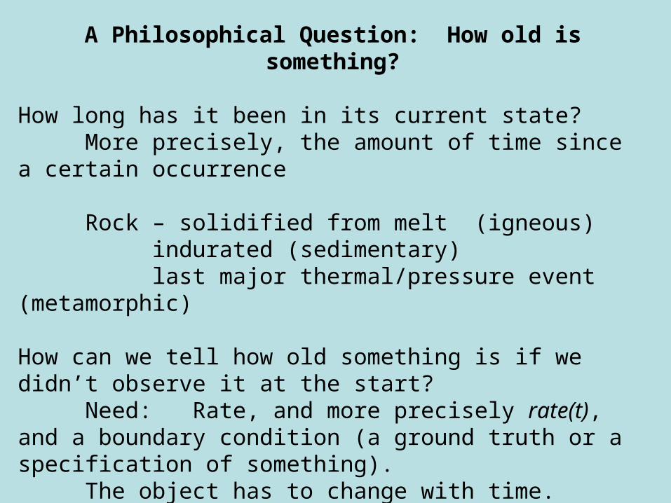
How we do this:
1. Relative (Geological) time scale: superposition, other simple physical rules.
Hutton – “no vestige of a beginning, no prospect of an end”Geologists use uniformity – 100’s of millions of years based on sedimentary evidence.
James Hutton and his unconformity
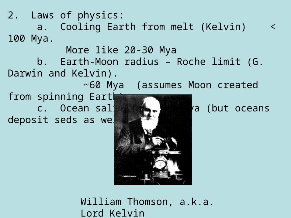
2. Laws of physics:a. Cooling Earth from melt (Kelvin) < 100 Mya.
More like 20-30 Myab. Earth-Moon radius – Roche limit (G. Darwin and Kelvin).
~60 Mya (assumes Moon created from spinning Earth)c. Ocean salinity ~ 100 Mya (but oceans deposit seds as
well).
William Thomson, a.k.a. Lord Kelvin
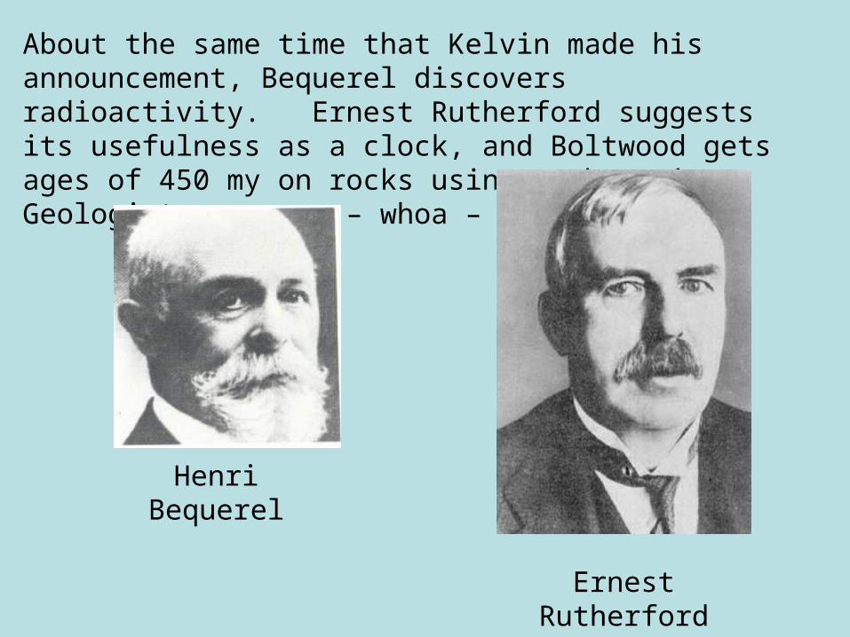
About the same time that Kelvin made his announcement, Bequerel discovers radioactivity. Ernest Rutherford suggests its usefulness as a clock, and Boltwood gets ages of 450 my on rocks using U/Pb ratios. Geologists now say – whoa – too old!
Ernest Rutherford
Henri Bequerel
The elements that make up matter are mostly stable, but a few (typically those with two many or too few neutrons in the nucleus – these are called isotopes), decay into other type of matter, releasing or absorbing energy and particles as they do so. This is called radioactive decay.
For example, carbon has isotopes of weight 12, 13, and 14 times the mass of a proton, and we refer to them as carbon-12, carbon-13, or carbon-14 (abbreviated as 12C, 13C, 14C). It is only the 14C isotope that is radioactive.
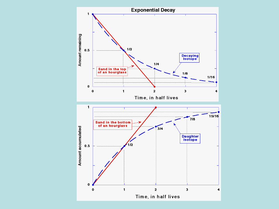
If there are a lot of atoms of the original element, called the parent or radioactive element, the atoms decay to another element, called the daughter or radiogenic element, at a predictable rate. The passage of time can be charted by the reduction in the number of parent atoms, and the increase in the number of daughter atoms.
How Radioactive Age Dating Works
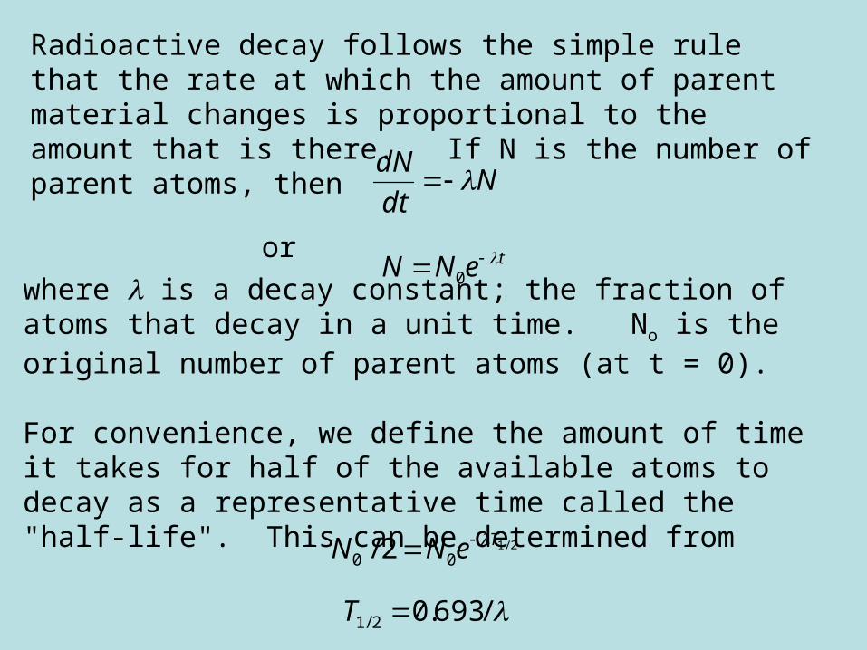
Radioactive decay follows the simple rule that the rate at which the amount of parent material changes is proportional to the amount that is there. If N is the number of parent atoms, then
Ndt
dN
teNN 0
or
where is a decay constant; the fraction of atoms that decay in a unit time. No is the original number of parent atoms (at t = 0).
For convenience, we define the amount of time it takes for half of the available atoms to decay as a representative time called the "half-life". This can be determined from
2/100 2/ TeNN
/693.02/1 T
So what do you need to know?
Well, if you can count all of the radioactive and radiogenic atoms in a rock, you could add them together to get No .
You know N, and if you also know the half-life (or, equivalently, the decay constant), the only thing left to determine is t.
What about a preexisting daughter product?
Note we have assumed that there is no daughter product in the original formation of the rock (or mineral, if we are dating a certain mineral). In some cases this assumption is ok, for example because the radioactive and radiogenic atoms are different sizes and only one is likely to be the right size to fit in a given mineral.
Well, that may be true in some instances, but is not true in general.
What to do?
In fact this is not so difficult. All you do is subtract off the initial concentration and get an equation where the time dependence is linear.
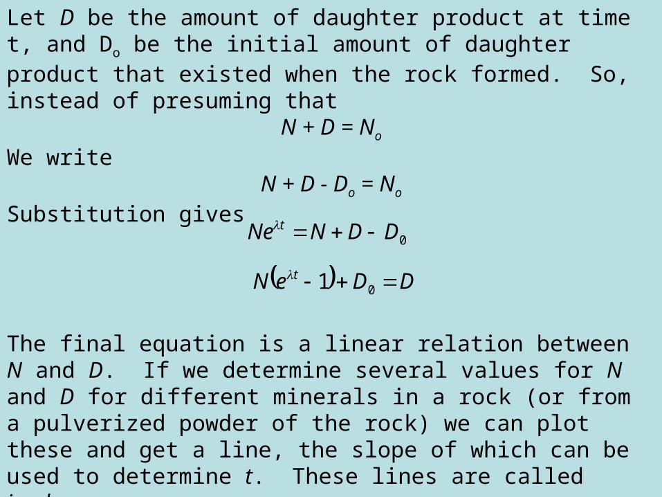
Let D be the amount of daughter product at time t, and Do be the initial amount of daughter product that existed when the rock formed. So, instead of presuming that
N + D = No
We write N + D - Do = No
Substitution gives
0DDNNe t
The final equation is a linear relation between N and D. If we determine several values for N and D for different minerals in a rock (or from a pulverized powder of the rock) we can plot these and get a line, the slope of which can be used to determine t. These lines are called isochrons.
DDeN t 01
The Radiometric Clocks
There are now well over forty different radiometric dating techniques, each based on a different radioactive isotope.
There is a large range in the half-lives of naturally occurring isotopes. Isotopes with long half-lives are useful for dating very old events. Isotopes with shorter half-lives cannot date very ancient events because all of the atoms of the parent isotope would have already decayed away, but are useful for dating correspondingly shorter intervals.
The uncertainties on the half-lives determined are all better than about two percent. There is no evidence of any of the half-lives changing over time.
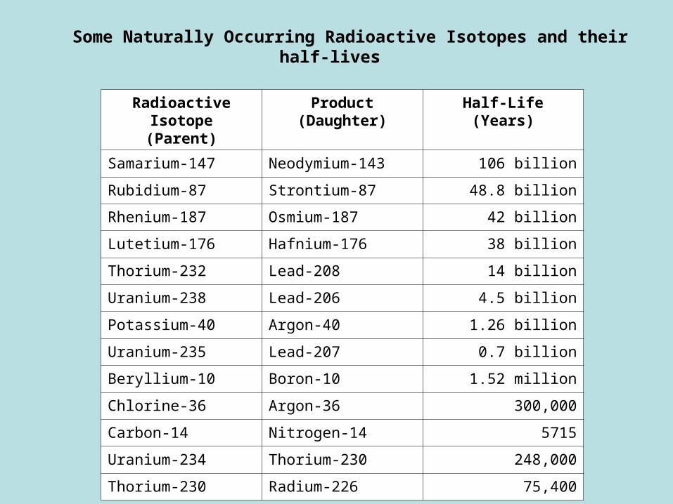
Some Naturally Occurring Radioactive Isotopes and their half-lives
Radioactive Isotope(Parent)
Product(Daughter)
Half-Life(Years)
Samarium-147 Neodymium-143 106 billion
Rubidium-87 Strontium-87 48.8 billion
Rhenium-187 Osmium-187 42 billion
Lutetium-176 Hafnium-176 38 billion
Thorium-232 Lead-208 14 billion
Uranium-238 Lead-206 4.5 billion
Potassium-40 Argon-40 1.26 billion
Uranium-235 Lead-207 0.7 billion
Beryllium-10 Boron-10 1.52 million
Chlorine-36 Argon-36 300,000
Carbon-14 Nitrogen-14 5715
Uranium-234 Thorium-230 248,000
Thorium-230 Radium-226 75,400
Examples of Dating Methods for Igneous Rocks
For igneous rocks the event being dated is when the rock was formed from magma or lava. When the molten material cools and hardens, the atoms are no longer free to move about.
Daughter atoms that result from radioactive decays occurring after the rock cools are frozen in the place where they were made within the rock.
Potassium-Argon (K-Ar) Method Potassium (K) is an abundant element in the Earth's crust. One isotope, 40K, is radioactive and decays to two different daughter products, 40Ca and 40Ar, by two different decay methods. This is not a problem because the production ratio of these two daughter products is precisely known, and is always constant: 11.2% becomes 40Ar and 88.8% becomes 40Ca.
It is possible to date some rocks by the K-Ca method, but this is not often done because it is hard to determine how much calcium was initially present.
Argon, on the other hand, is a gas. Whenever rock is melted to become magma or lava, the argon tends to escape. Once the molten material hardens, it begins to trap the new argon produced since the hardening took place. In this way the potassium-argon clock is reset when an igneous rock is formed.
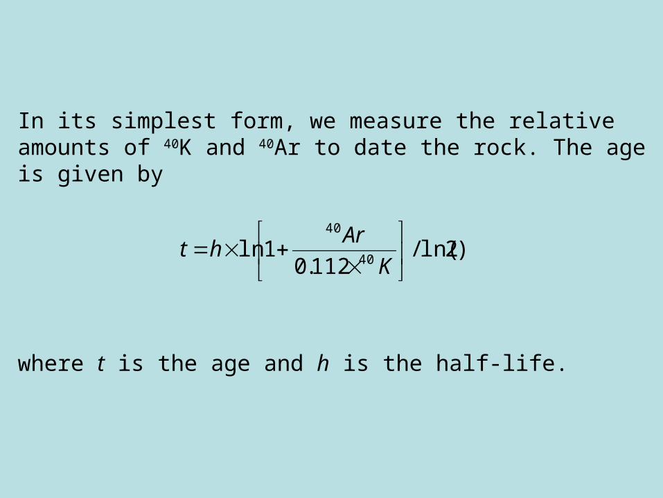
In its simplest form, we measure the relative amounts of 40K and 40Ar to date the rock. The age is given by
)2ln(/112.0
1ln40
40
K
Arht
where t is the age and h is the half-life.
However, in reality there is often a small amount of argon remaining in a rock when it hardens. This is usually trapped in the form of very tiny air bubbles in the rock.
One must have a way to determine how much air-Ar is in the rock. One approach is to recognize that argon has a couple of other isotopes, the most abundant of which is 36Ar.
The ratio of 40Ar to 36Ar in air is known to be 295. Thus, if one measures 36Ar as well as 40Ar, one can calculate and subtract off the air-40Ar to get an accurate age.
Even so, Ar is sometimes contaminated with gas from deep underground rather than from the air. This gas can have a higher concentration of 40Ar escaping from the melting of older rocks. This is called parentless 40Ar because its parent potassium is not in the rock being dated, and is also not from the air. In these cases, the date given by the normal potassium-argon method is too old.
Because of all these difficulties, K-Ar is not used much except in special circumstances. Still, scientists in the mid-1960s came up with a way to use ratios of argon isotopes to produce very reliable ages. This is called the Ar-Ar method.
The Argon-Argon method
This technique uses the ratio 40Ar/39Ar to estimate age. It has become quite popular in recent years because it appears to be quite robust and precise.
39Ar is unstable and does not exist in nature because its half life is only 269 years. Its daughter is 39K. 39K is stable, and because 39A has such a short half-life, for all intents all naturally occurring 39K can be considered non-radiogenic.
But that means that if we make our own 39Ar then the amount will be stable over the duration of our experiments (usually several days).
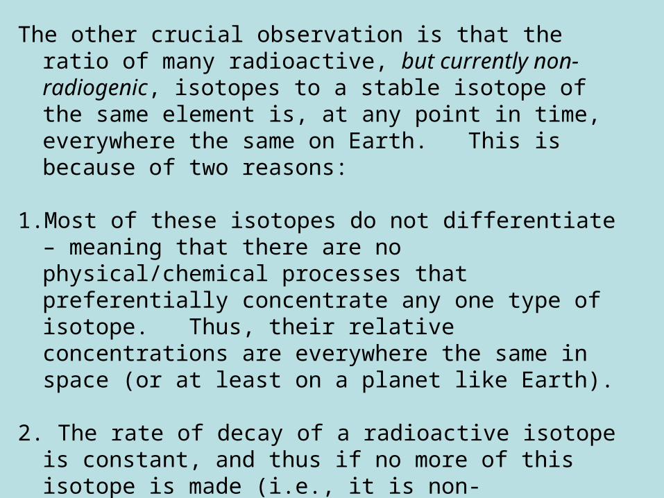
The other crucial observation is that the ratio of many radioactive, but currently non-radiogenic, isotopes to a stable isotope of the same element is, at any point in time, everywhere the same on Earth. This is because of two reasons:
1. Most of these isotopes do not differentiate – meaning that there are no physical/chemical processes that preferentially concentrate any one type of isotope. Thus, their relative concentrations are everywhere the same in space (or at least on a planet like Earth).
2. The rate of decay of a radioactive isotope is constant, and thus if no more of this isotope is made (i.e., it is non-radiogenic), then it is reducing at the same rate everywhere.
Thus, even though 40K is radioactive, neither it nor 39K is currently radiogenic, so the ratio 40K/39K is, at any particular time, the same everywhere (and hence in every rock).
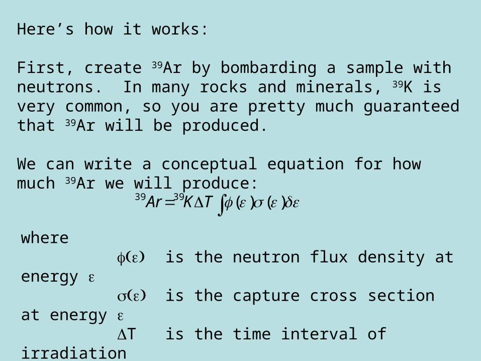
Here’s how it works:
First, create 39Ar by bombarding a sample with neutrons. In many rocks and minerals, 39K is very common, so you are pretty much guaranteed that 39Ar will be produced.
We can write a conceptual equation for how much 39Ar we will produce:
)()(3939 TKAr
where is the neutron flux density at energy is the capture cross section at energy T is the time interval of irradiation
and the integral is over all possible energy levels.
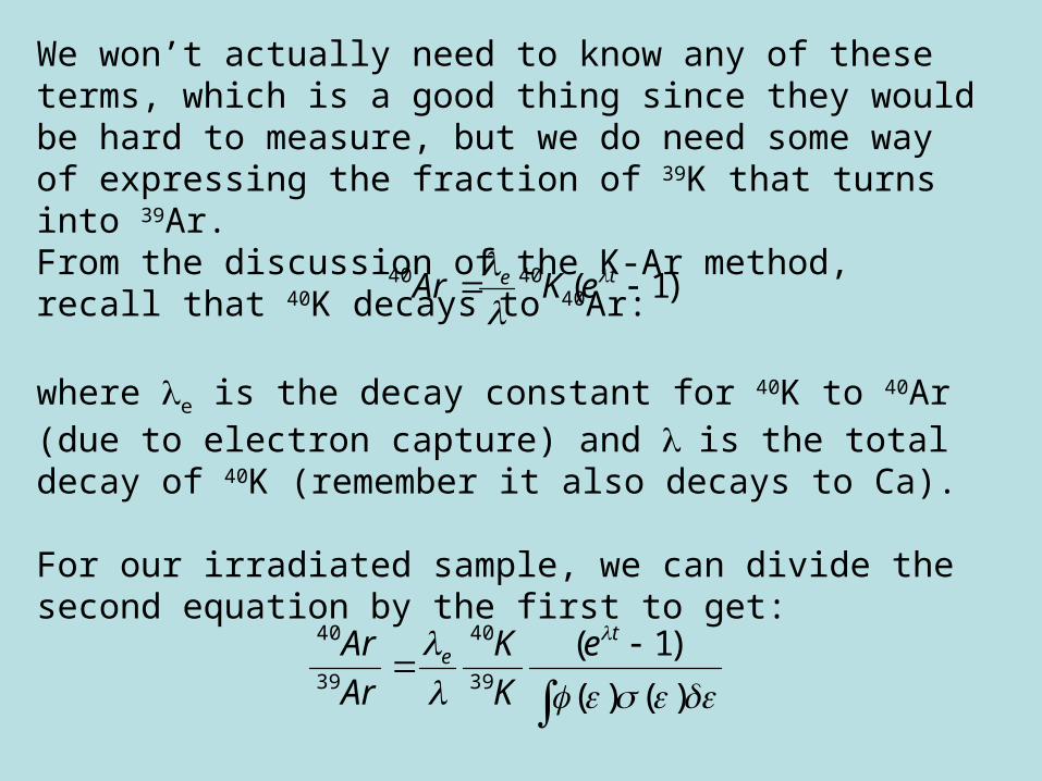
We won’t actually need to know any of these terms, which is a good thing since they would be hard to measure, but we do need some way of expressing the fraction of 39K that turns into 39Ar.From the discussion of the K-Ar method, recall that 40K decays to 40Ar:
)1(4040 te eKAr
where e is the decay constant for 40K to 40Ar (due to electron capture) and is the total decay of 40K (remember it also decays to Ca). For our irradiated sample, we can divide the second equation by the first to get:
)()(
)1(39
40
39
40 te e
K
K
Ar
Ar
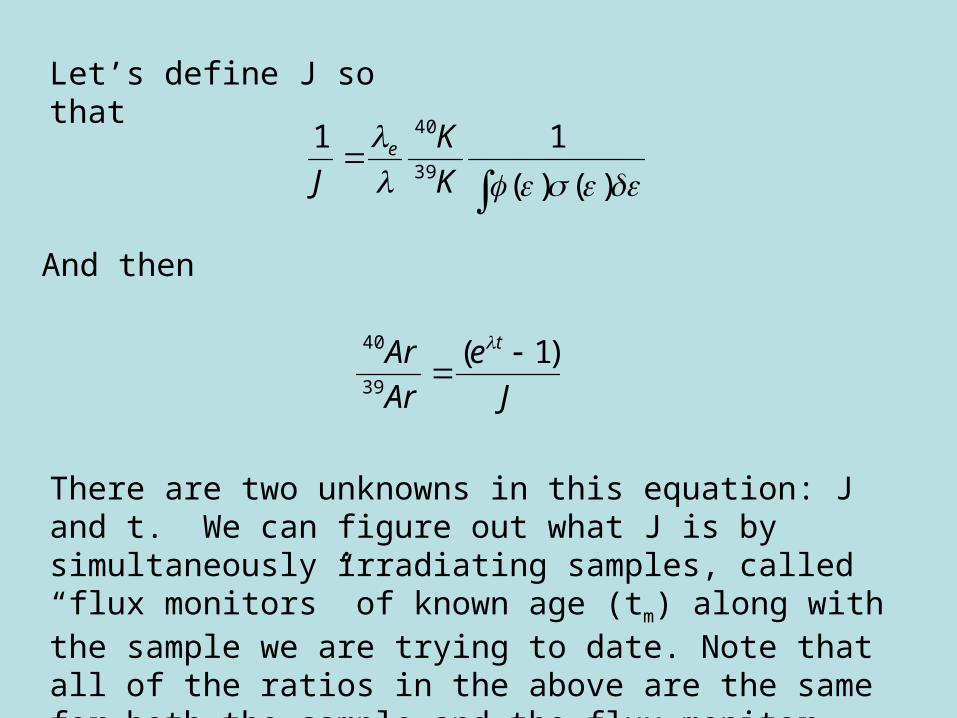
Let’s define J so that
)()(
1139
40
K
K
Je
J
e
Ar
Ar t )1(39
40
And then
There are two unknowns in this equation: J and t. We can figure out what J is by simultaneously irradiating samples, called “flux monitors” of known age (tm) along with the sample we are trying to date. Note that all of the ratios in the above are the same for both the sample and the flux monitor, and hence J is the same for both.
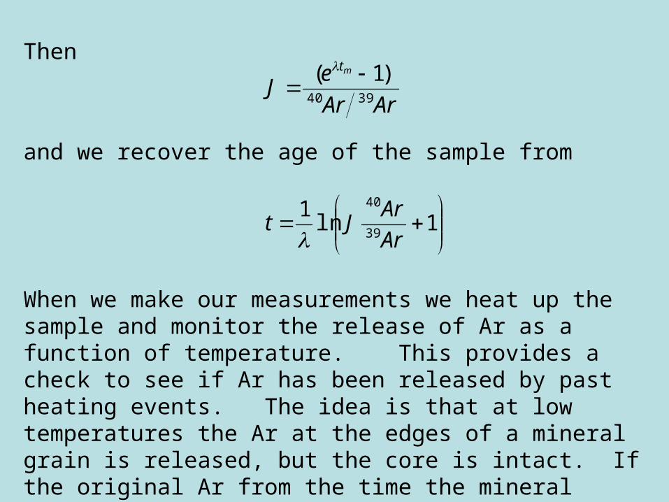
Then
ArAr
eJ
mt
3940
)1(
and we recover the age of the sample from
1ln
139
40
Ar
ArJt
When we make our measurements we heat up the sample and monitor the release of Ar as a function of temperature. This provides a check to see if Ar has been released by past heating events. The idea is that at low temperatures the Ar at the edges of a mineral grain is released, but the core is intact. If the original Ar from the time the mineral cooled and became a closed system is retained, then the 40Ar/39Ar ratio will be independent of temperature or “plateau”.
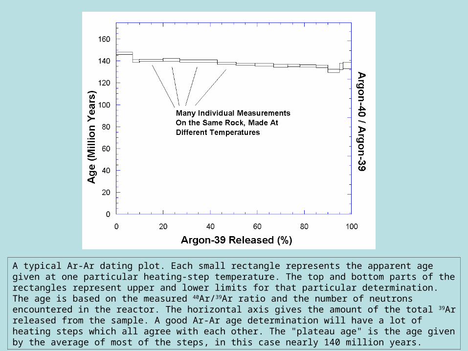
A typical Ar-Ar dating plot. Each small rectangle represents the apparent age given at one particular heating-step temperature. The top and bottom parts of the rectangles represent upper and lower limits for that particular determination. The age is based on the measured 40Ar/39Ar ratio and the number of neutrons encountered in the reactor. The horizontal axis gives the amount of the total 39Ar released from the sample. A good Ar-Ar age determination will have a lot of heating steps which all agree with each other. The "plateau age" is the age given by the average of most of the steps, in this case nearly 140 million years.
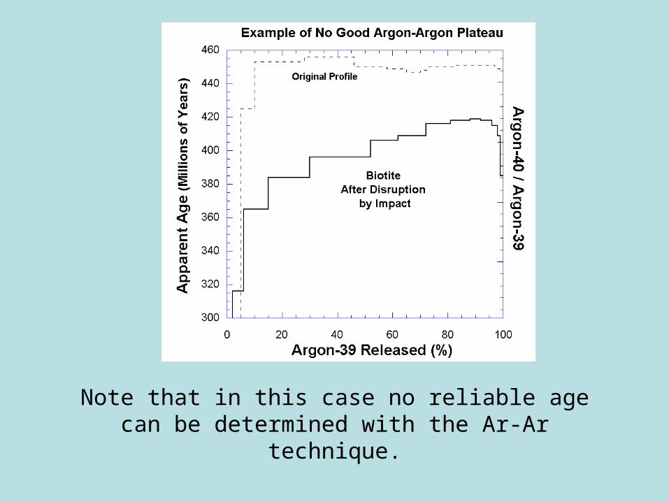
Note that in this case no reliable age can be determined with the Ar-Ar technique.
Rubidium-Strontium (Rb-Sr)
Rb-Sr provides a good example of how to handle pre-existing daughter products.
In the Rb-Sr method, 87Rb decays with a half-life of 48.8 billion years to 87Sr. Strontium has several other isotopes that are stable. The ratio of 87Sr to one of the other stable isotopes, say 86Sr, increases over time as more 87Rb turns to 87Sr.
But when the rock first cools, all parts of the rock have the same 87Sr/86Sr ratio because the isotopes were mixed in the magma. At the same time, some of the minerals in the rock have a higher initial Rb/Sr ratio than others. Rubidium has a larger atomic diameter than strontium, so rubidium does not fit into the crystal structure of some minerals as well as others.
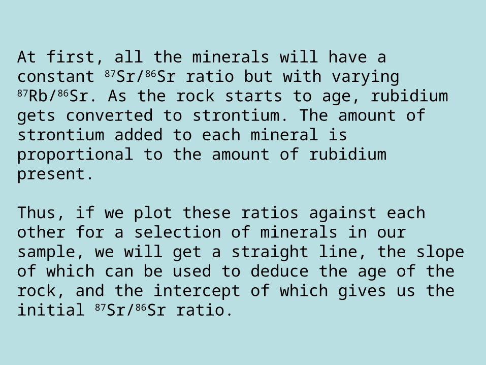
At first, all the minerals will have a constant 87Sr/86Sr ratio but with varying 87Rb/86Sr. As the rock starts to age, rubidium gets converted to strontium. The amount of strontium added to each mineral is proportional to the amount of rubidium present.
Thus, if we plot these ratios against each other for a selection of minerals in our sample, we will get a straight line, the slope of which can be used to deduce the age of the rock, and the intercept of which gives us the initial 87Sr/86Sr ratio.

A rubidium-strontium three-isotope plot. When a rock cools, all its minerals have the same ratio of 87Sr to 86Sr, though they have varying amounts of rubidium. As the rock ages, the rubidium decreases by changing to 87Sr, as shown by the dotted arrows. Minerals with more rubidium gain more 87Sr, while those with less rubidium do not change as much. Notice that at any given time, the minerals all line up--a check to ensure that the system has not been disturbed.
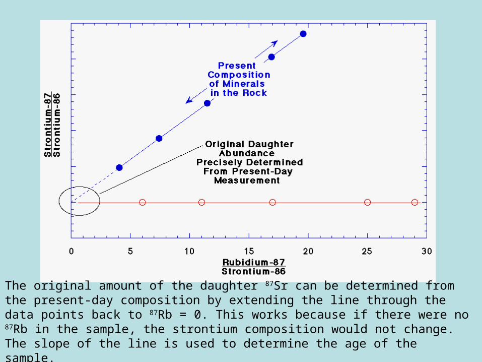
The original amount of the daughter 87Sr can be determined from the present-day composition by extending the line through the data points back to 87Rb = 0. This works because if there were no 87Rb in the sample, the strontium composition would not change. The slope of the line is used to determine the age of the sample.
The Samarium-Neodymium, Lutetium-Hafnium, and Rhenium-Osmium Methods
All of these methods work very similarly to the rubidium-strontium method.
The samarium-neodymium method is the most-often used of these three. It uses the decay of samarium-147 to neodymium-143, which has a half-life of 105 billion years. The ratio of the daughter isotope, neodymium-143, to another neodymium isotope, neodymium-144, is plotted against the ratio of the parent, samarium-147, to neodymium-144.
The samarium-neodymium method has been shown to be more resistant to being disturbed or reset by metamorphic heating events, so for some metamorphosed rocks the samarium-neodymium method is preferred.
The lutetium-hafnium method uses the 38 billion year half-life of lutetium-176 decaying to hafnium-176. This dating system is similar in many ways to samarium-neodymium, but since samarium-neodymium dating is somewhat easier, the lutetium-hafnium method is used less often.
The rhenium-osmium method takes advantage of the very low osmium concentration in most rocks and minerals, so that a small amount of the parent rhenium-187 can produce a significant change in the osmium isotope ratio. The half-life for this radioactive decay is 42 billion years. The non-radiogenic stable isotopes, osmium-186 or -188, are used as the denominator in the ratios on the three-isotope plots.
This method has been useful for dating iron meteorites, and is now enjoying greater use for dating Earth rocks due to development of easier rhenium and osmium isotope measurement techniques.
Uranium-Lead and related techniques (U-Pb)
The uranium-lead method is the longest-used dating method. It was first used by Boltwood in 1907, about a century ago.
The uranium-lead system is more complicated than other parent-daughter systems; it is actually several dating methods put together.
Natural uranium consists primarily of two isotopes, 235U and 238U, and these isotopes decay with different half-lives to produce 207Pb and 206Pb, respectively.
In addition, 208Pb is produced by thorium-232. Only one isotope of lead, 204Pb, is not radiogenic.
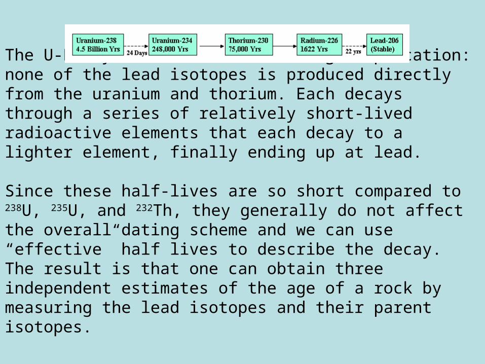
The U-Pb system has an interesting complication: none of the lead isotopes is produced directly from the uranium and thorium. Each decays through a series of relatively short-lived radioactive elements that each decay to a lighter element, finally ending up at lead.
Since these half-lives are so short compared to 238U, 235U, and 232Th, they generally do not affect the overall dating scheme and we can use “effective” half lives to describe the decay. The result is that one can obtain three independent estimates of the age of a rock by measuring the lead isotopes and their parent isotopes.
The uranium-lead system in its simpler forms, using 238U, 235U, and 232Th, has proved to be less reliable than many of the other dating systems. This is because both U and Pb are less easily retained in many of the minerals in which they are found.
Yet the fact that there are three dating systems all in one allows us to determine whether the system has been disturbed or not.
One of the techniques used to do determine the time of a reset event is called the U-Pb Condordia technique.
Notes on U-Pb Concordia and Discordia
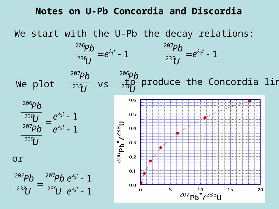
We start with the U-Pb the decay relations:
206Pb238U
e1t 1
207Pb235U
e2t 1
We plot
206Pb238U vs
207Pb235U
to produce the Concordia line:
206Pb238U
207Pb235U
e1t 1
e2t 1
or
206Pb238U
207Pb235U
e1t 1
e2t 1
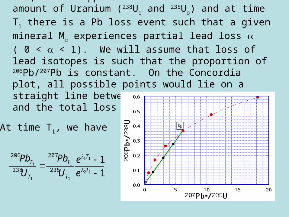
Now, let’s suppose we start out with the some amount of Uranium (238Uo and 235Uo) and at time T1 there is a Pb loss event such that a
given mineral M experiences partial lead loss ( 0 < < 1). We
will assume that loss of lead isotopes is such that the proportion of 206Pb/207Pb is constant. On the Concordia plot, all possible points would lie on a straight line between the no-loss condition and the total loss condition.
At time T1, we have
206PbT1
238UT1
207PbT1
235UT1
e1T1 1
e2T1 1
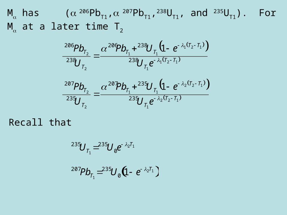
M has (206PbT1, 207PbT1,238UT1, and 235UT1). For M at a later time T2
121
1
121
11
2
2
238
238206
238
206 1TT
T
TTTT
T
T
eU
eUPb
U
Pb
122
1
122
11
2
2
235
235207
235
207 1TT
T
TTTT
T
T
eU
eUPb
U
Pb
Recall that
235UT1235U0e
2T1
207PbT1235U0 1 e 2T1
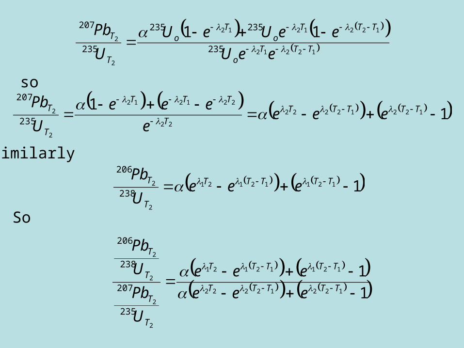
so
12212
1221212
2
2
235
235235
235
20711
TTTo
TTTo
To
T
T
eeU
eeUeU
U
Pb
11
12212222
22
221212
2
2
235
207
TTTTT
T
TTT
T
T eeee
eee
U
Pb
Similarly
112112121
2
2
238
206
TTTTT
T
T eeeU
Pb
So
1
112212222
12112121
2
2
2
2
235
207
238
206
TTTTT
TTTTT
T
T
T
T
eee
eee
U
Pb
U
Pb
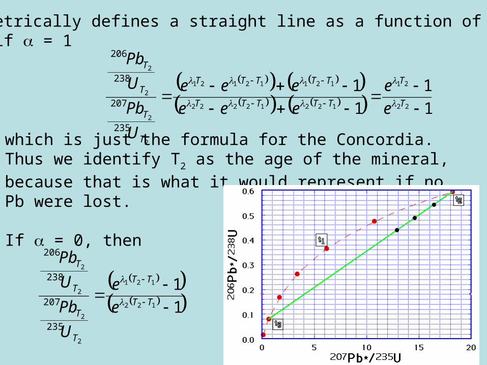
This parametrically defines a straight line as a function of . Note that if = 1
1
1
1
122
21
12212222
12112121
2
2
2
2
235
207
238
206
T
T
TTTTT
TTTTT
T
T
T
T
e
e
eee
eee
U
Pb
U
Pb
which is just the formula for the Concordia. Thus we identify T2 as
the age of the mineral, because that is what it would represent if no Pb were lost.
If = 0, then
1
1122
121
2
2
2
2
235
207
238
206
TT
TT
T
T
T
T
e
e
U
Pb
U
Pb
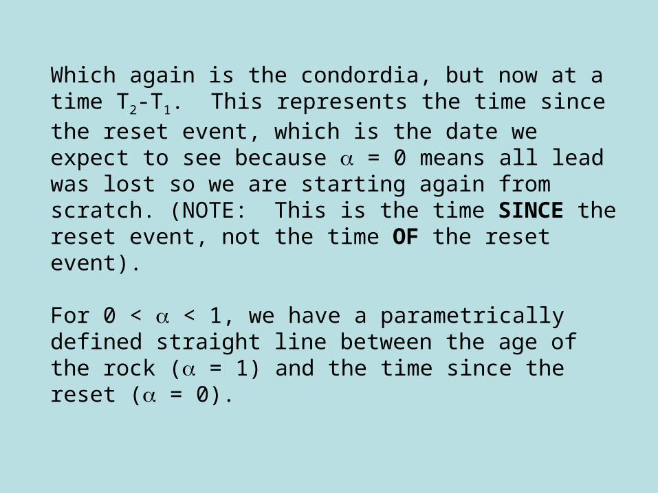
Which again is the condordia, but now at a time T2-T1. This represents the time since the reset event, which is the date we expect to see because = 0 means all lead was lost so we are starting again from scratch. (NOTE: This is the time SINCE the reset event, not the time OF the reset event).
For 0 < < 1, we have a parametrically defined straight line between the age of the rock ( = 1) and the time since the reset ( = 0).
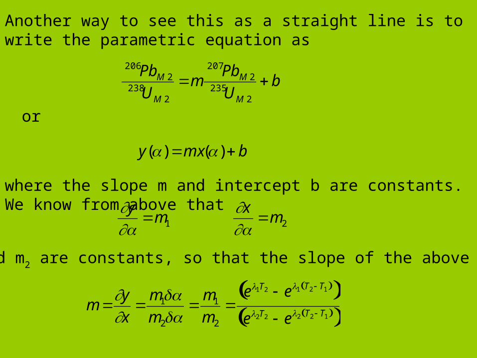
Another way to see this as a straight line is to write the parametric equation as
206PbM 2238UM 2
m207PbM 2235UM 2
b
or
y() mx() b
where the slope m and intercept b are constants. We know from above that
y
m1
x
m2
where m1 and m2 are constants, so that the slope of the above line is
m y
x
m1m2
m1
m2
e1T2 e1 T2 T1 e2T2 e2 T2 T1
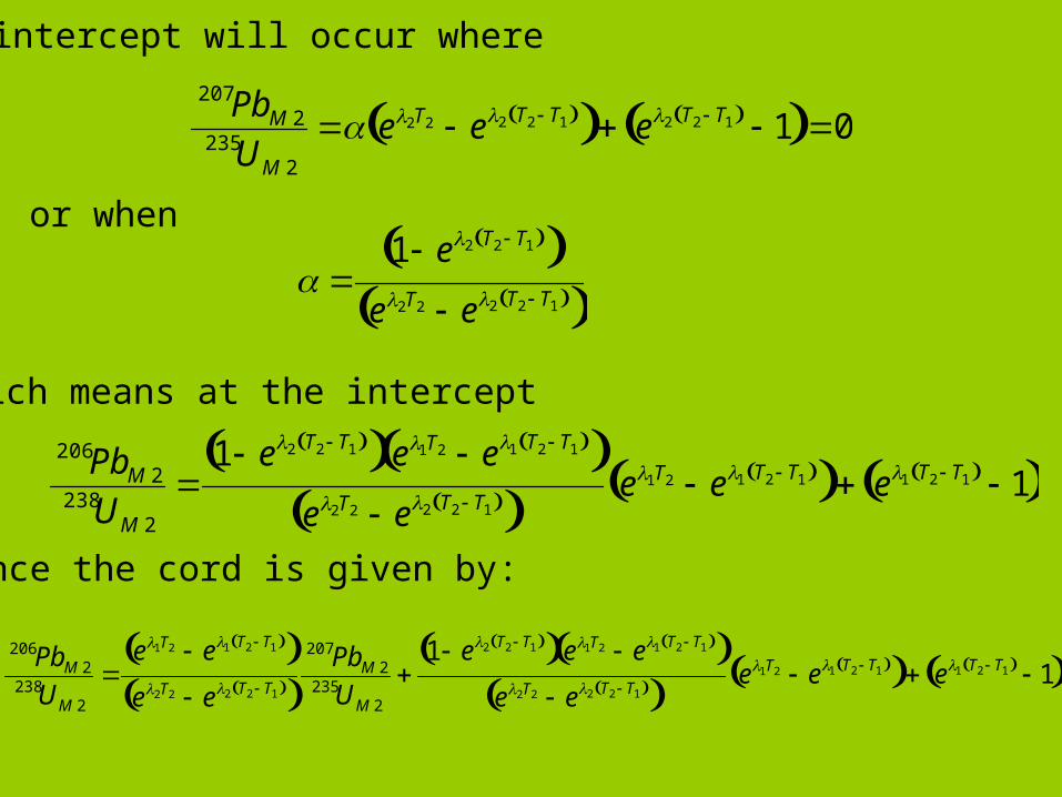
The intercept will occur where
207PbM 2235UM 2
e2T2 e2 T2 T1 e2 T2 T1 1 0
or when
1 e2 T2 T1
e2T2 e2 T2 T1 which means at the intercept
206PbM 2238UM 2
1 e2 T2 T1 e1T2 e1 T2 T1
e2T2 e2 T2 T1 e1T2 e1 T2 T1 e1 T2 T1 1 Hence the cord is given by:
206PbM 2238UM 2
e1T2 e1 T2 T1 e2T2 e2 T2 T1
207PbM 2235UM 2
1 e2 T2 T1 e1T2 e1 T2 T1
e2T2 e2 T2 T1 e1T2 e1 T2 T1 e1 T2 T1 1
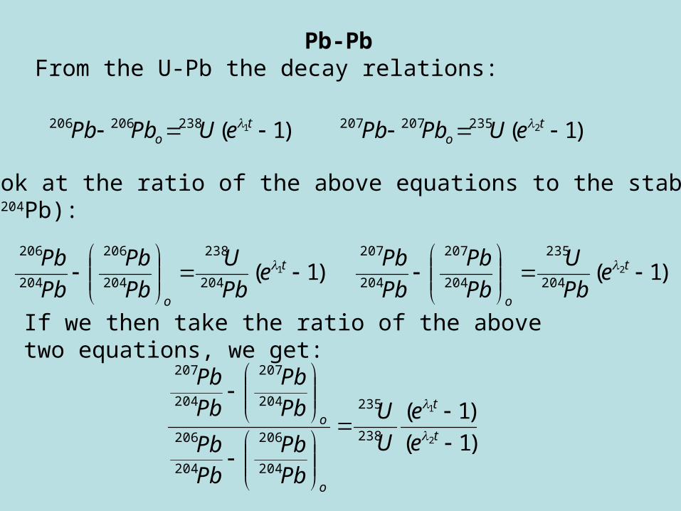
Pb-PbFrom the U-Pb the decay relations:
)1( 1238206206 to eUPbPb )1( 2235207207 t
o eUPbPb
We can look at the ratio of the above equations to the stable isotopeof Lead (204Pb):
If we then take the ratio of the above two equations, we get:
)1( 1
204
238
204
206
204
206
t
o
ePb
U
Pb
Pb
Pb
Pb )1( 2
204
235
204
207
204
207
t
o
ePb
U
Pb
Pb
Pb
Pb
)1(
)1(2
1
238
235
204
206
204
206
204
207
204
207
t
t
o
o
e
e
U
U
PbPb
PbPb
PbPb
PbPb
The ratio
ooPb
Pb
Pb
Pbm
Pb
Pb
Pb
Pb204
206
204
206
204
207
204
207
88.137
1238
235
U
U
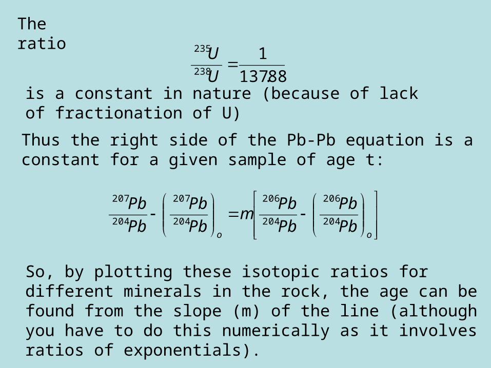
is a constant in nature (because of lack of fractionation of U)
Thus the right side of the Pb-Pb equation is a constant for a given sample of age t:
So, by plotting these isotopic ratios for different minerals in the rock, the age can be found from the slope (m) of the line (although you have to do this numerically as it involves ratios of exponentials).
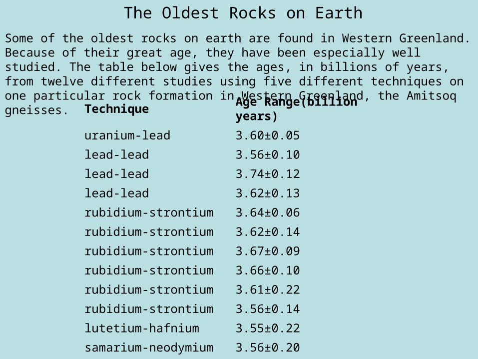
Some of the oldest rocks on earth are found in Western Greenland. Because of their great age, they have been especially well studied. The table below gives the ages, in billions of years, from twelve different studies using five different techniques on one particular rock formation in Western Greenland, the Amitsoq gneisses.
Technique Age Range(billion years)
uranium-lead 3.60±0.05
lead-lead 3.56±0.10
lead-lead 3.74±0.12
lead-lead 3.62±0.13
rubidium-strontium 3.64±0.06
rubidium-strontium 3.62±0.14
rubidium-strontium 3.67±0.09
rubidium-strontium 3.66±0.10
rubidium-strontium 3.61±0.22
rubidium-strontium 3.56±0.14
lutetium-hafnium 3.55±0.22
samarium-neodymium 3.56±0.20
The Oldest Rocks on Earth
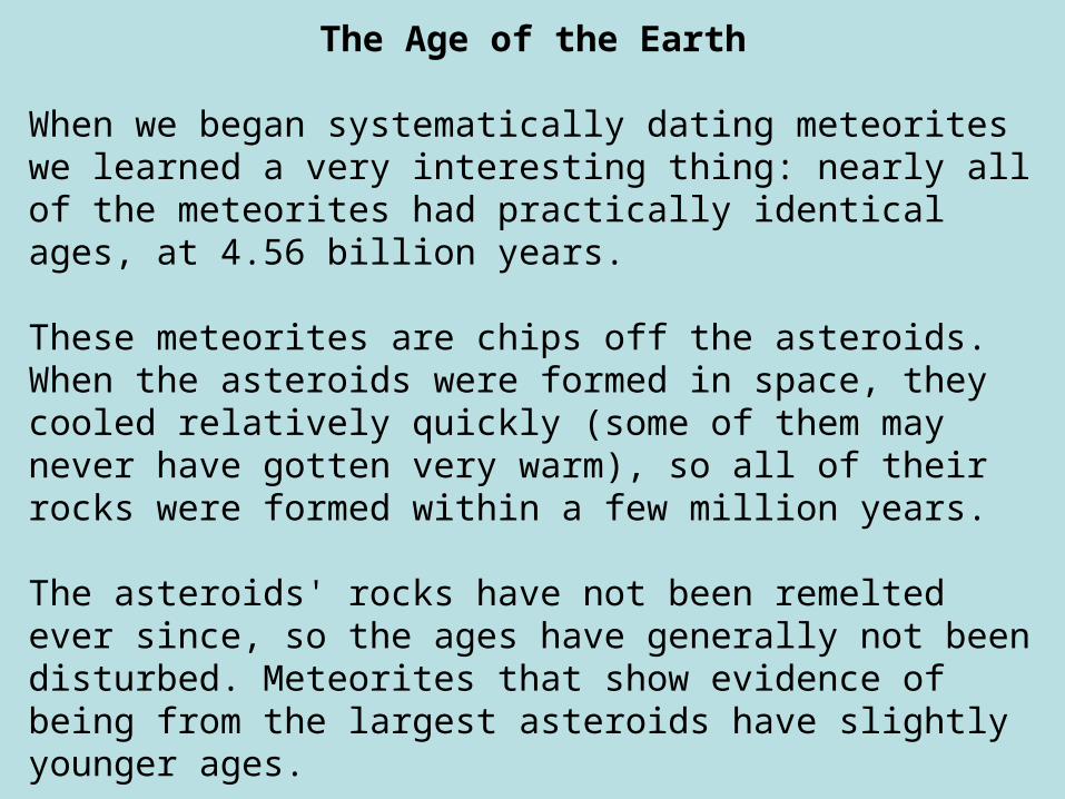
The Age of the Earth
When we began systematically dating meteorites we learned a very interesting thing: nearly all of the meteorites had practically identical ages, at 4.56 billion years.
These meteorites are chips off the asteroids. When the asteroids were formed in space, they cooled relatively quickly (some of them may never have gotten very warm), so all of their rocks were formed within a few million years.
The asteroids' rocks have not been remelted ever since, so the ages have generally not been disturbed. Meteorites that show evidence of being from the largest asteroids have slightly younger ages.
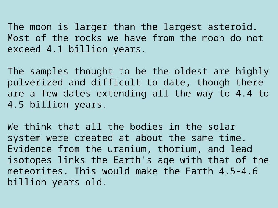
The moon is larger than the largest asteroid. Most of the rocks we have from the moon do not exceed 4.1 billion years.
The samples thought to be the oldest are highly pulverized and difficult to date, though there are a few dates extending all the way to 4.4 to 4.5 billion years.
We think that all the bodies in the solar system were created at about the same time. Evidence from the uranium, thorium, and lead isotopes links the Earth's age with that of the meteorites. This would make the Earth 4.5-4.6 billion years old.
Extinct Radionuclides: The Hourglasses That Ran Out
If we find that a radioactive parent was once abundant but has since run out, we know that it too was set longer ago than the time interval it measures. In fact, most of them are no longer found naturally on Earth--they have run out.
Their half-lives range down to times shorter than we can measure. Every single element has radioisotopes that no longer exist on Earth!
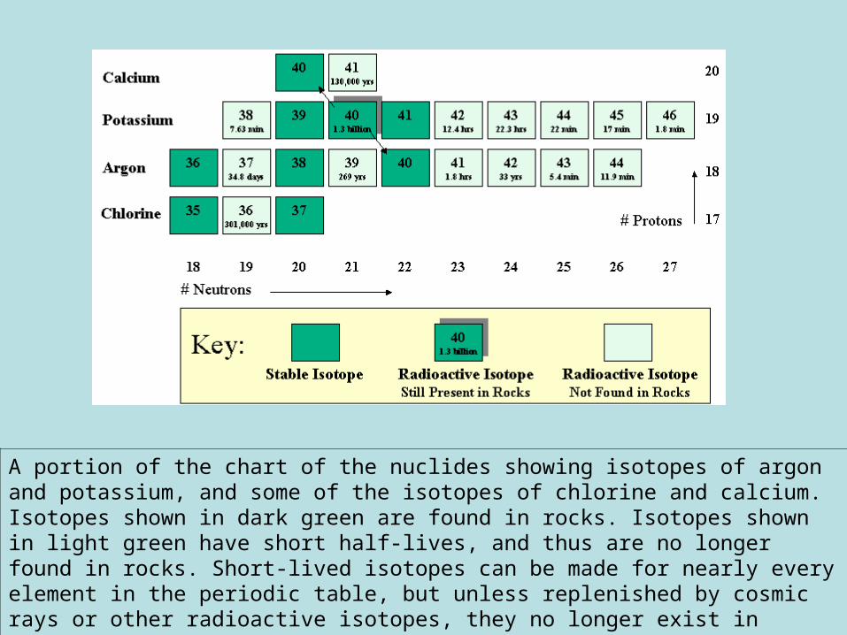
A portion of the chart of the nuclides showing isotopes of argon and potassium, and some of the isotopes of chlorine and calcium. Isotopes shown in dark green are found in rocks. Isotopes shown in light green have short half-lives, and thus are no longer found in rocks. Short-lived isotopes can be made for nearly every element in the periodic table, but unless replenished by cosmic rays or other radioactive isotopes, they no longer exist in nature.
Cosmogenic Radionuclides: Carbon-14, Beryllium-10, Chlorine-36
Unlike the radioactive isotopes discussed above, these isotopes are constantly being replenished in small amounts by cosmic rays--high energy particles and photons in space--as they hit the Earth's upper atmosphere.
Very small amounts of each of these isotopes are present in the air we breathe and the water we drink. As a result, living things, both plants and animals, ingest very small amounts of carbon-14, and lake and sea sediments take up small amounts of beryllium-10 and chlorine-36.
The cosmogenic dating clocks work somewhat differently than the others. 14C is created by radiation of 14N in the atmosphere, but we do not use the decay of 14C back to 14N when using it as a dating tool.
We assume (and we’ll get back to this in a bit) that to a good approximation, the ratio of 14C to the stable isotopes, 12C and 13C, is relatively constant in the atmosphere and living organisms.
Once a living thing dies, it no longer takes in carbon from food or air, and the amount of 14C starts to drop with time. The carbon-14C/12C ratio indicates how old the sample is.
Since the half-life of 14C is less than 6,000 years, it can only be used for dating material less than about 45,000 years old. Thus, dinosaur bones do not have 14C (unless contaminated), but some other animals that are now extinct, such as North American mammoths, can be dated by 14C.
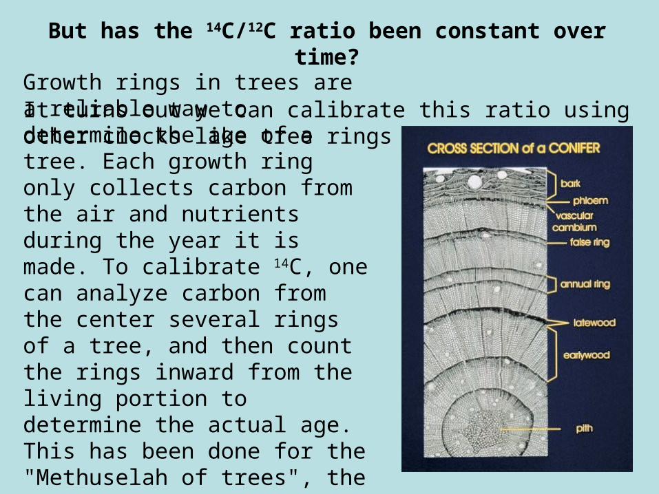
But has the 14C/12C ratio been constant over time?
It turns out we can calibrate this ratio using other clocks like tree rings and stalactites.
Growth rings in trees are a reliable way to determine the age of a tree. Each growth ring only collects carbon from the air and nutrients during the year it is made. To calibrate 14C, one can analyze carbon from the center several rings of a tree, and then count the rings inward from the living portion to determine the actual age. This has been done for the "Methuselah of trees", the bristlecone pine trees, which grow very slowly and live up to 6,000 years.
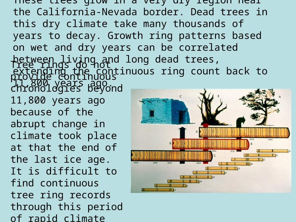
These trees grow in a very dry region near the California-Nevada border. Dead trees in this dry climate take many thousands of years to decay. Growth ring patterns based on wet and dry years can be correlated between living and long dead trees, extending the continuous ring count back to 11,800 years ago.
Tree rings do not provide continuous chronologies beyond 11,800 years ago because of the abrupt change in climate took place at that the end of the last ice age. It is difficult to find continuous tree ring records through this period of rapid climate change.
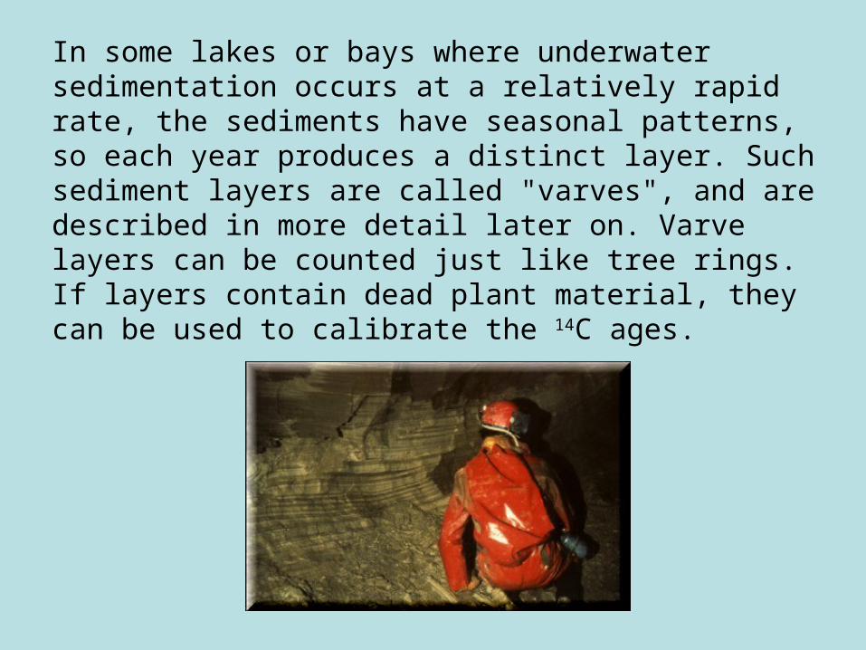
In some lakes or bays where underwater sedimentation occurs at a relatively rapid rate, the sediments have seasonal patterns, so each year produces a distinct layer. Such sediment layers are called "varves", and are described in more detail later on. Varve layers can be counted just like tree rings. If layers contain dead plant material, they can be used to calibrate the 14C ages.
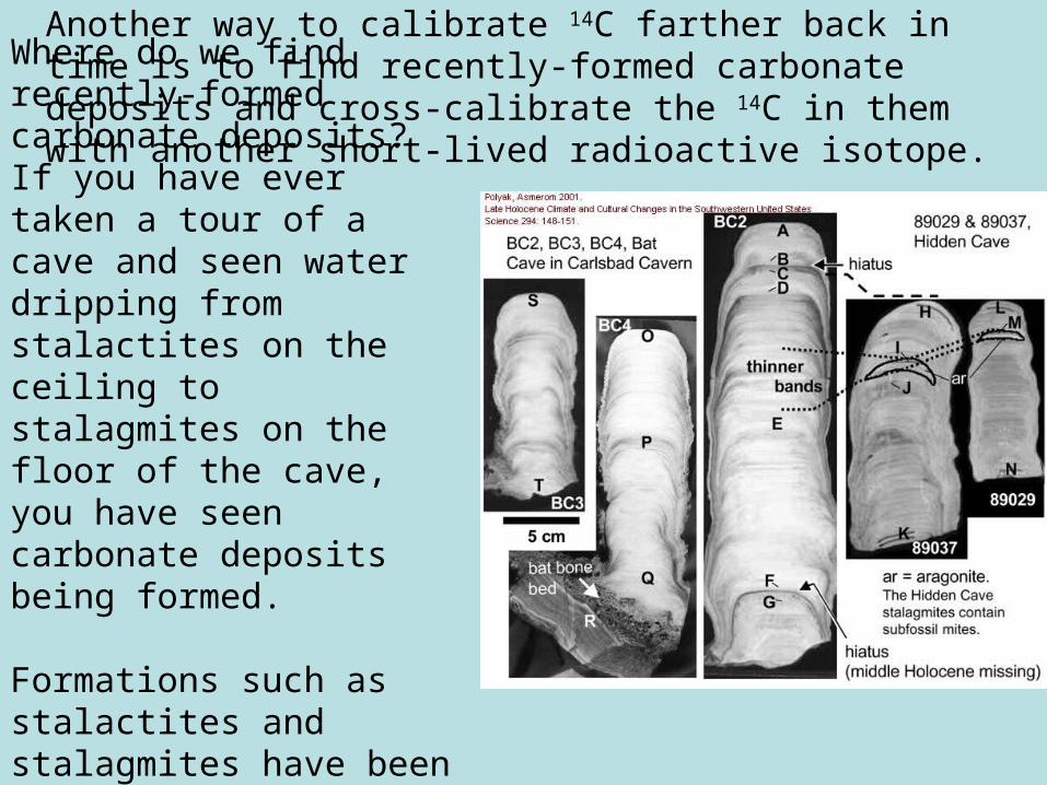
Another way to calibrate 14C farther back in time is to find recently-formed carbonate deposits and cross-calibrate the 14C in them with another short-lived radioactive isotope.
Where do we find recently-formed carbonate deposits? If you have ever taken a tour of a cave and seen water dripping from stalactites on the ceiling to stalagmites on the floor of the cave, you have seen carbonate deposits being formed.
Formations such as stalactites and stalagmites have been quite useful in cross-calibrating the 14C record.
What does one find in the calibration of 14C against actual ages?
We find that the 14C fraction in the air has decreased over the last 40,000 years by about a factor of two. This is attributed to a strengthening of the Earth's magnetic field during this time. A stronger magnetic field shields the upper atmosphere better from charged cosmic rays, resulting in less 14C production now than in the past.
A small amount of data beyond 40,000 years suggests that this trend reversed between 40,000 and 50,000 years, with lower 14C/12C ratios farther back in time, but these data are preliminary.
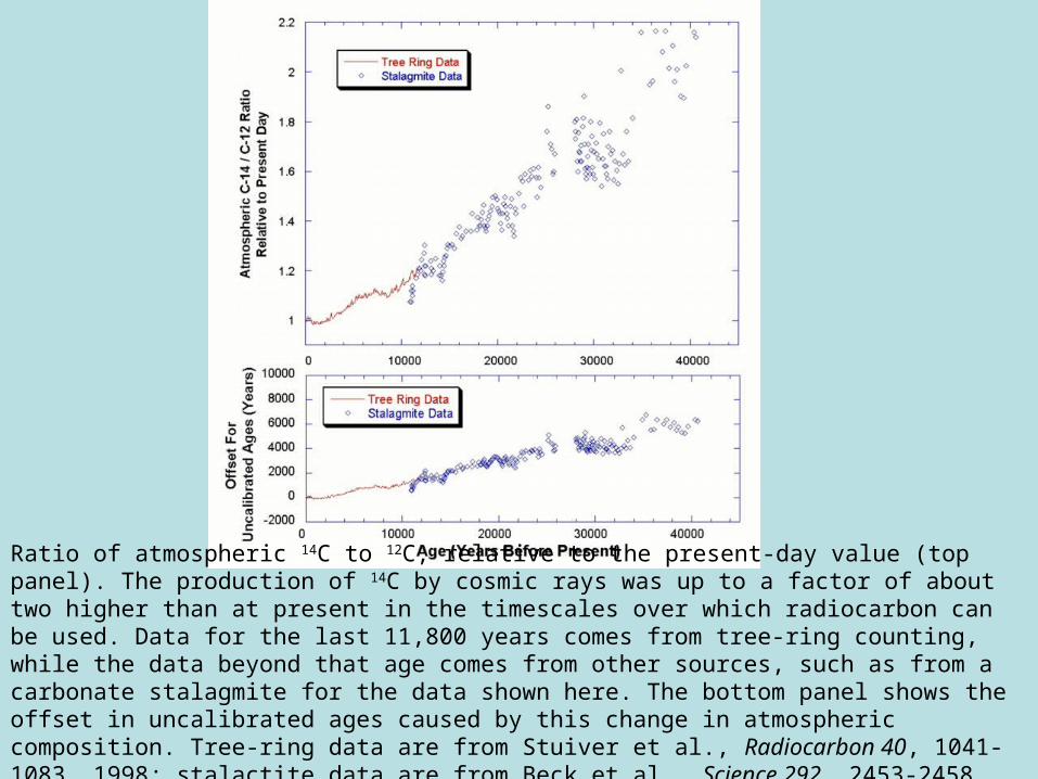
Ratio of atmospheric 14C to 12C, relative to the present-day value (top panel). The production of 14C by cosmic rays was up to a factor of about two higher than at present in the timescales over which radiocarbon can be used. Data for the last 11,800 years comes from tree-ring counting, while the data beyond that age comes from other sources, such as from a carbonate stalagmite for the data shown here. The bottom panel shows the offset in uncalibrated ages caused by this change in atmospheric composition. Tree-ring data are from Stuiver et al., Radiocarbon 40, 1041-1083, 1998; stalactite data are from Beck et al., Science 292, 2453-2458, 2001.
Radiometric Dating of Geologically Young Samples (<100,000 Years)
It is sometimes possible to date geologically young samples using some of the long-lived methods described above. These methods may work on young samples, for example, if there is a relatively high concentration of the parent isotope in the sample. In that case, sufficient daughter isotope amounts are produced in a relatively short time.
As an example, the argon-argon method has been used successfully to recover the known age of lava from the famous eruption of Vesuvius in Italy in 79 A.D.
Short-lived radionuclides produced by decay of the long-lived radionuclides: U-Th.
As mentioned in the U-Pb section, uranium does not decay immediately to a stable isotope, but decays through a number of shorter-lived radioisotopes until it ends up as lead. While the uranium-lead system can measure intervals in the millions of years generally without problems from the intermediate isotopes, those intermediate isotopes with the longest half-lives span long enough time intervals for dating events less than several hundred thousand years ago.
Two of the most frequently-used of these "uranium-series" systems are 234U and 230Th.
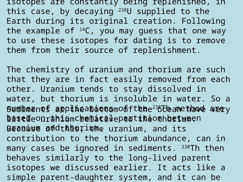
Like 14C, the shorter-lived uranium-series isotopes are constantly being replenished, in this case, by decaying 238U supplied to the Earth during its original creation. Following the example of 14C, you may guess that one way to use these isotopes for dating is to remove them from their source of replenishment.
The chemistry of uranium and thorium are such that they are in fact easily removed from each other. Uranium tends to stay dissolved in water, but thorium is insoluble in water. So a number of applications of the 230Th method are based on this chemical partition between uranium and thorium.
Sediments at the bottom of the ocean have very little uranium relative to the thorium. Because of this, the uranium, and its contribution to the thorium abundance, can in many cases be ignored in sediments. 230Th then behaves similarly to the long-lived parent isotopes we discussed earlier. It acts like a simple parent-daughter system, and it can be used to date sediments.
On the other hand, calcium carbonates produced biologically (such as in corals, shells, teeth, and bones) take in small amounts of uranium, but essentially no thorium (because of its much lower concentrations in the water). This allows the dating of these materials by their lack of thorium.
Comparison of 234U ages with ages obtained by counting annual growth bands of corals proves that the technique is highly accurate when properly used. The method has also been used to date stalactites and stalagmites from caves, already mentioned in connection with long-term calibration of the 14C method. Tens of thousands of U-Th dates have been performed on cave formations around the world.
Counting Coral Rings
The 234U - 230Th method is now being used to date animal and human bones and teeth.
Work to date shows that dating of tooth enamel can be quite reliable. However, dating of bones can be more problematic, as bones are more susceptible to contamination by the surrounding soils.
Non-Radiometric Dating Methods for the Past 100,000 Years
We will digress briefly from radiometric dating to talk about other dating techniques. A very large number of accurate dates covering the past 100,000 years has been obtained from many other methods besides radiometric dating. We have already mentioned dendrochronology (tree ring dating) above. Here we will look briefly at some other non-radiometric dating techniques.
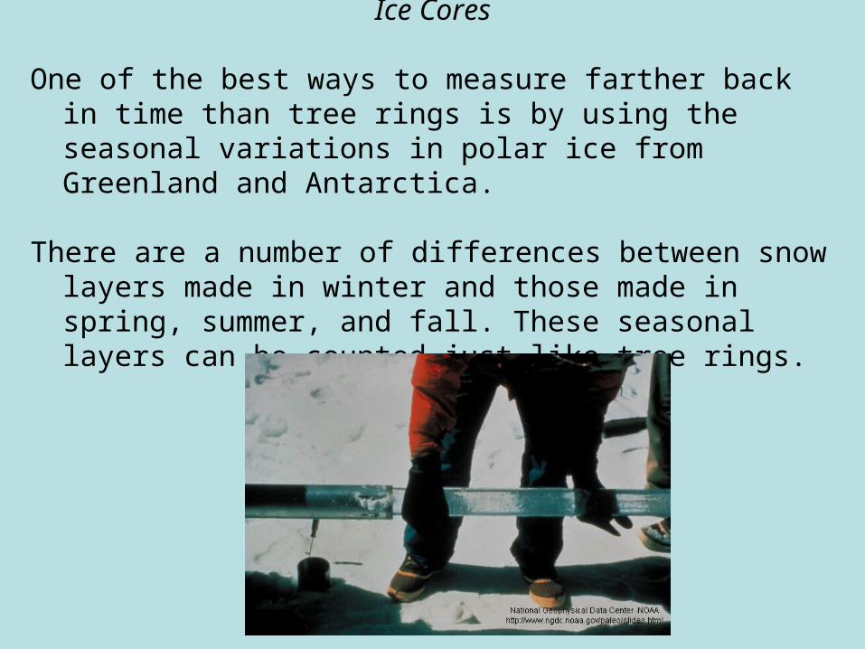
Ice Cores
One of the best ways to measure farther back in time than tree rings is by using the seasonal variations in polar ice from Greenland and Antarctica.
There are a number of differences between snow layers made in winter and those made in spring, summer, and fall. These seasonal layers can be counted just like tree rings.
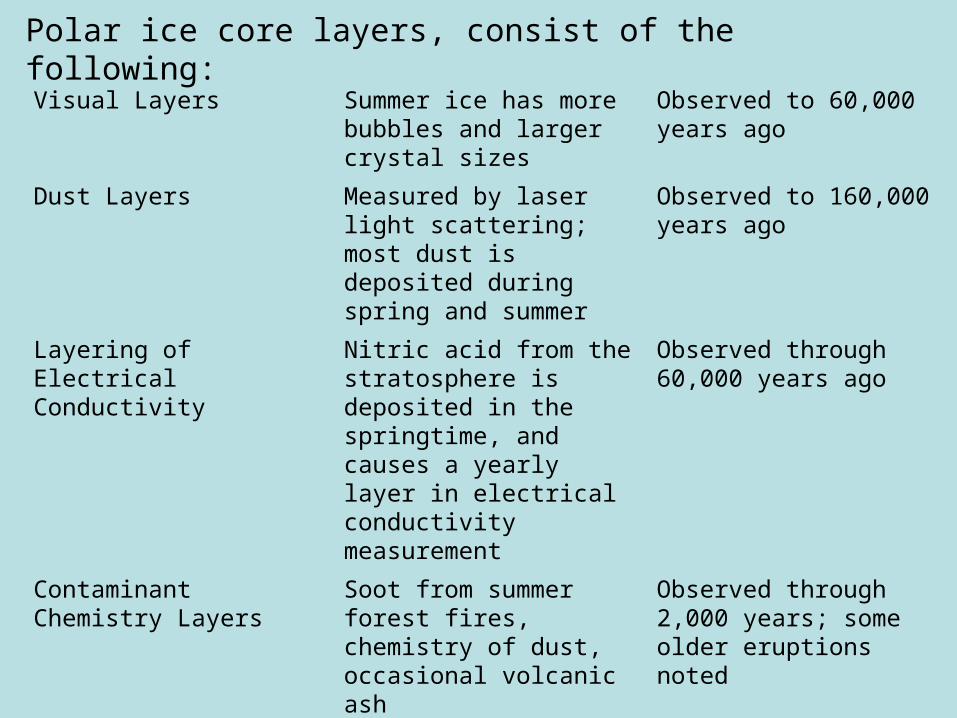
Visual Layers Summer ice has more bubbles and larger crystal sizes
Observed to 60,000 years ago
Dust Layers Measured by laser light scattering; most dust is deposited during spring and summer
Observed to 160,000 years ago
Layering of Electrical Conductivity
Nitric acid from the stratosphere is deposited in the springtime, and causes a yearly layer in electrical conductivity measurement
Observed through 60,000 years ago
Contaminant Chemistry Layers
Soot from summer forest fires, chemistry of dust, occasional volcanic ash
Observed through 2,000 years; some older eruptions noted
Hydrogen and Oxygen Isotope Layering
Indicates temperature of precipitation. Heavy isotopes (oxygen-18 and deuterium) are depleted more in winter.
Yearly layers observed through 1,100 years; Trends observed much farther back in time
Polar ice core layers, consist of the following:
A continuous count of layers exists back as far as 160,000 years.
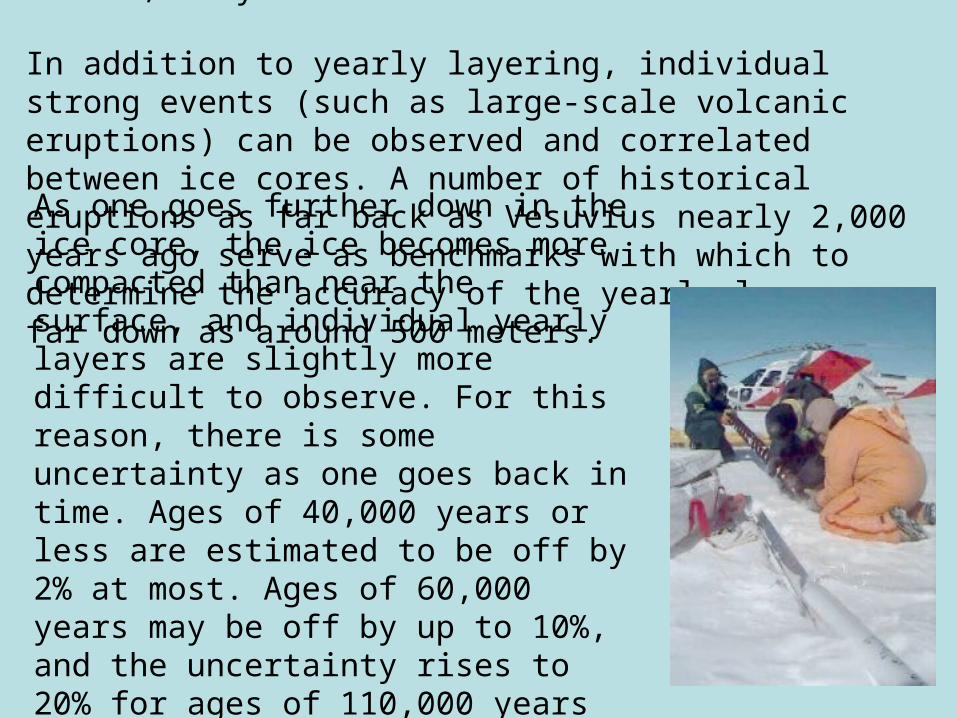
In addition to yearly layering, individual strong events (such as large-scale volcanic eruptions) can be observed and correlated between ice cores. A number of historical eruptions as far back as Vesuvius nearly 2,000 years ago serve as benchmarks with which to determine the accuracy of the yearly layers as far down as around 500 meters.
As one goes further down in the ice core, the ice becomes more compacted than near the surface, and individual yearly layers are slightly more difficult to observe. For this reason, there is some uncertainty as one goes back in time. Ages of 40,000 years or less are estimated to be off by 2% at most. Ages of 60,000 years may be off by up to 10%, and the uncertainty rises to 20% for ages of 110,000 years based on direct counting of layers.
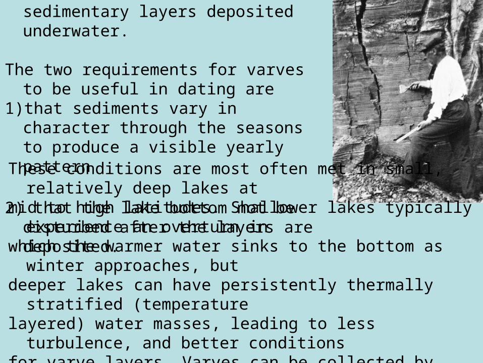
Varves. Another layering technique uses seasonal variations in sedimentary layers deposited underwater.
The two requirements for varves to be useful in dating are
1) that sediments vary in character through the seasons to produce a visible yearly pattern
2) that the lake bottom not be disturbed after the layers are deposited.
These conditions are most often met in small, relatively deep lakes at mid to high latitudes. Shallower lakes typically experience an overturn inwhich the warmer water sinks to the bottom as winter approaches, butdeeper lakes can have persistently thermally stratified (temperaturelayered) water masses, leading to less turbulence, and better conditionsfor varve layers. Varves can be collected by coring drills, somewhatlike of ice cores.
Each yearly varve layer consists of
a) mineral matter brought in by swollen streams in the spring.
b) This gradually gives way to organic particulate matter such as plant fibers, algae, and pollen with fine-grained mineral matter, consistent with summer and fall deposition.
c) With winter ice covering the lake, fine-grained organic matter provides the final part of the yearly layer.
Regular sequences of varves have been measured going back to about 35,000 years. The thicknesses of the layers and the types of material in them tells a lot about the climate of the time when the layers were deposited. For example, pollens entrained in the layers can tell what types of plants were growing nearby at a particular time.
Other annual layering methods
Besides tree rings, ice cores, and sediment varves, there are other processes that result in yearly layers that can be counted to determine an age.
Annual layering in coral reefs can be used to date sections of coral. Coral generally grows at rates of around 1 cm per year, and these layers are easily visible. As was mentioned in the uranium-series section, the counting of annual coral layers was used to verify the accuracy of the thorium-230 method.
Thermoluminescence. There is a way of dating minerals and pottery that does not rely directly on half-lives. Thermoluminescence dating, or TL dating, uses the fact that radioactive decays cause some electrons in a material to end up stuck in higher-energy orbits. The number of electrons in higher-energy orbits accumulates as a material experiences more natural radioactivity over time. If the material is heated, these electrons can fall back to their original orbits, emitting a very tiny amount of light. If the heating occurs in a laboratory furnace equipped with a very sensitive light detector, this light can be recorded. (The term comes from putting together thermo, meaning heat, and luminescence, meaning to emit light).
By comparison of the amount of light emitted with the natural radioactivity rate the sample experienced, the age of the sample can be determined. TL dating can generally be used on samples less than half a million years old. Related techniques include optically stimulated luminescence (OSL), and infrared stimulated luminescence (IRSL). TL dating and its related techniques have been cross calibrated with samples of known historical age and with radiocarbon and thorium dating. While TL dating does not usually pinpoint the age with as great an accuracy as these other conventional radiometric dating, it is most useful for applications such as pottery or fine-grained volcanic dust, where other dating methods do not work as well.
Electron spin resonance (ESR).
Also called electron paramagnetic resonance, ESR dating also relies on the changes in electron orbits and spins caused by radioactivity over time. However, ESR dating can be used over longer time periods, up to two million years, and works best on carbonates, such as in coral reefs and cave deposits. It has also seen extensive use in dating tooth enamel
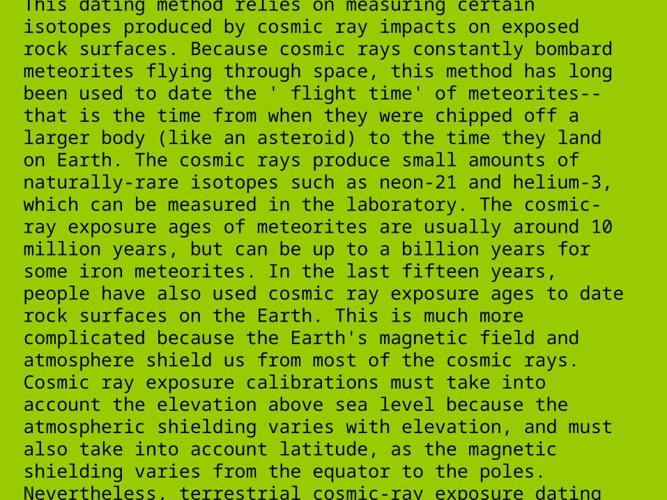
Cosmic-ray exposure dating. This dating method relies on measuring certain isotopes produced by cosmic ray impacts on exposed rock surfaces. Because cosmic rays constantly bombard meteorites flying through space, this method has long been used to date the ' flight time' of meteorites--that is the time from when they were chipped off a larger body (like an asteroid) to the time they land on Earth. The cosmic rays produce small amounts of naturally-rare isotopes such as neon-21 and helium-3, which can be measured in the laboratory. The cosmic-ray exposure ages of meteorites are usually around 10 million years, but can be up to a billion years for some iron meteorites. In the last fifteen years, people have also used cosmic ray exposure ages to date rock surfaces on the Earth. This is much more complicated because the Earth's magnetic field and atmosphere shield us from most of the cosmic rays. Cosmic ray exposure calibrations must take into account the elevation above sea level because the atmospheric shielding varies with elevation, and must also take into account latitude, as the magnetic shielding varies from the equator to the poles. Nevertheless, terrestrial cosmic-ray exposure dating has been shown to be useful in many cases.
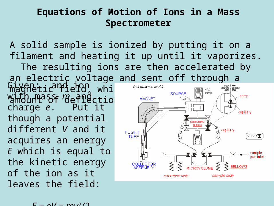
Equations of Motion of Ions in a Mass Spectrometer
A solid sample is ionized by putting it on a filament and heating it up until it vaporizes. The resulting ions are then accelerated by an electric voltage and sent off through a magnetic field, which deflects them. The amount of deflection identifies the ion.
Given: and ion with mass m and charge e. Put it though a potential different V and it acquires an energy E which is equal to the kinetic energy of the ion as it leaves the field:
E = eV = mv2/2
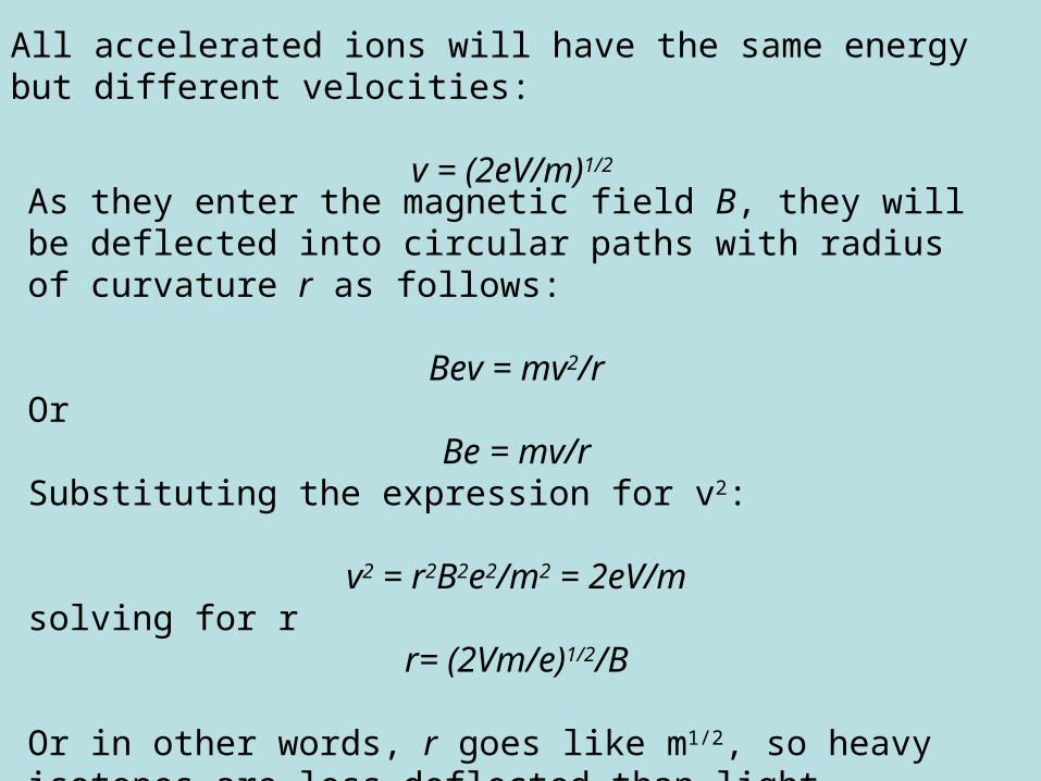
As they enter the magnetic field B, they will be deflected into circular paths with radius of curvature r as follows:
Bev = mv2/rOr
Be = mv/rSubstituting the expression for v2:
v2 = r2B2e2/m2 = 2eV/msolving for r
r= (2Vm/e)1/2/B
Or in other words, r goes like m1/2, so heavy isotopes are less deflected than light isotopes for a given field strength.
All accelerated ions will have the same energy but different velocities:
v = (2eV/m)1/2