Embed Size (px)
Citation preview
RC C
hakra
borty,
ww
w.m
yrea
ders.
info
Genetic Algorithms & Modeling : Soft Computing Course Lecture 37 – 40, notes, slides
www.myreaders.info/ , RC Chakraborty, e-mail [email protected] , Aug. 10, 2010
http://www.myreaders.info/html/soft_computing.html
Genetic Algorithms & Modeling
Soft Computing
Genetic algorithms & Modeling, topics : Introduction, why genetic
algorithm? search optimization methods, evolutionary algorithms
(EAs), genetic algorithms (GAs) - biological background, working
principles; basic genetic algorithm, flow chart for Genetic
Programming. Encoding : binary encoding, value encoding,
permutation encoding, tree encoding. Operators of genetic
algorithm : random population, reproduction or selection -
roulette wheel selection, Boltzmann selection; Fitness function;
Crossover - one-point crossover, two-point crossover, uniform
crossover, arithmetic, heuristic; Mutation - flip bit, boundary,
Gaussian, non-uniform, and uniform; Basic genetic algorithm :
examples - maximize function f(x) = x2 and two bar pendulum.
www.myreaders.info
RC C
hakra
borty,
ww
w.m
yrea
ders.
info
Genetic Algorithms & Modeling
Soft Computing
Topics
(Lectures 37, 38, 39, 40 4 hours)
Slides
1. Introduction
What are Genetic Algorithms and why Genetic Algorithm? Search
optimization methods; Evolutionary Algorithms (EAs), Genetic
Algorithms (GAs) : Biological background, Working principles, Basic
Genetic Algorithm, Flow chart for Genetic Programming.
03-23
2. Encoding
Binary Encoding, Value Encoding, Permutation Encoding, Tree
Encoding.
24-29
3. Operators of Genetic Algorithm
Random population, Reproduction or Selection : Roulette wheel
selection, Boltzmann selection; Fitness function; Crossover: One-point
crossover, Two-point crossover, Uniform crossover, Arithmetic,
Heuristic; Mutation: Flip bit, Boundary, Gaussian, Non-uniform, and
Uniform;
30-43
4. Basic Genetic Algorithm
Examples : Maximize function f(x) = x2 and Two bar pendulum.
44-49
5. References
50
02
RC C
hakra
borty,
ww
w.m
yrea
ders.
info
Genetic Algorithms & Modeling
What are GAs ?
• Genetic Algorithms (GAs) are adaptive heuristic search algorithm based
on the evolutionary ideas of natural selection and genetics.
• Genetic algorithms (GAs) are a part of Evolutionary computing, a rapidly
growing area of artificial intelligence. GAs are inspired by Darwin's
theory about evolution - "survival of the fittest".
• GAs represent an intelligent exploitation of a random search used to
solve optimization problems.
• GAs, although randomized, exploit historical information to direct the
search into the region of better performance within the search space.
• In nature, competition among individuals for scanty resources results
in the fittest individuals dominating over the weaker ones.
03
RC C
hakra
borty,
ww
w.m
yrea
ders.
info
SC – GA - Introduction 1. Introduction
Solving problems mean looking for solutions, which is best among others.
Finding the solution to a problem is often thought :
− In computer science and AI, as a process of search through the space of
possible solutions. The set of possible solutions defines the search space
(also called state space) for a given problem. Solutions or partial solutions
are viewed as points in the search space.
− In engineering and mathematics, as a process of optimization. The
problems are first formulated as mathematical models expressed in terms
of functions and then to find a solution, discover the parameters that
optimize the model or the function components that provide optimal
system performance.
04
RC C
hakra
borty,
ww
w.m
yrea
ders.
info
SC – GA - Introduction • Why Genetic Algorithms ?
It is better than conventional AI ; It is more robust.
- unlike older AI systems, the GA's do not break easily even if the
inputs changed slightly, or in the presence of reasonable noise.
- while performing search in large state-space, multi-modal state-space,
or n-dimensional surface, a genetic algorithms offer significant benefits
over many other typical search optimization techniques like - linear
programming, heuristic, depth-first, breath-first.
"Genetic Algorithms are good at taking large, potentially huge search
spaces and navigating them, looking for optimal combinations of things,
the solutions one might not otherwise find in a lifetime.” Salvatore
Mangano Computer Design, May 1995.
05
RC C
hakra
borty,
ww
w.m
yrea
ders.
info
SC – GA - Introduction 1.1 Optimization
Optimization is a process that finds a best, or optimal, solution for a
problem. The Optimization problems are centered around three factors :
■ An objective function : which is to be minimized or maximized;
Examples: 1. In manufacturing, we want to maximize the profit or minimize
the cost . 2. In designing an automobile panel, we want to maximize the
strength. ■ A set of unknowns or variables : that affect the objective function,
Examples: 1. In manufacturing, the variables are amount of resources used or
the time spent. 2. In panel design problem, the variables are shape and dimensions of
the panel. ■ A set of constraints : that allow the unknowns to take on certain
values but exclude others;
Examples: 1. In manufacturing, one constrain is, that all "time" variables to
be non-negative. 2 In the panel design, we want to limit the weight and put
constrain on its shape.
An optimization problem is defined as : Finding values of the variables
that minimize or maximize the objective function while satisfying
the constraints. 06
RC C
hakra
borty,
ww
w.m
yrea
ders.
info
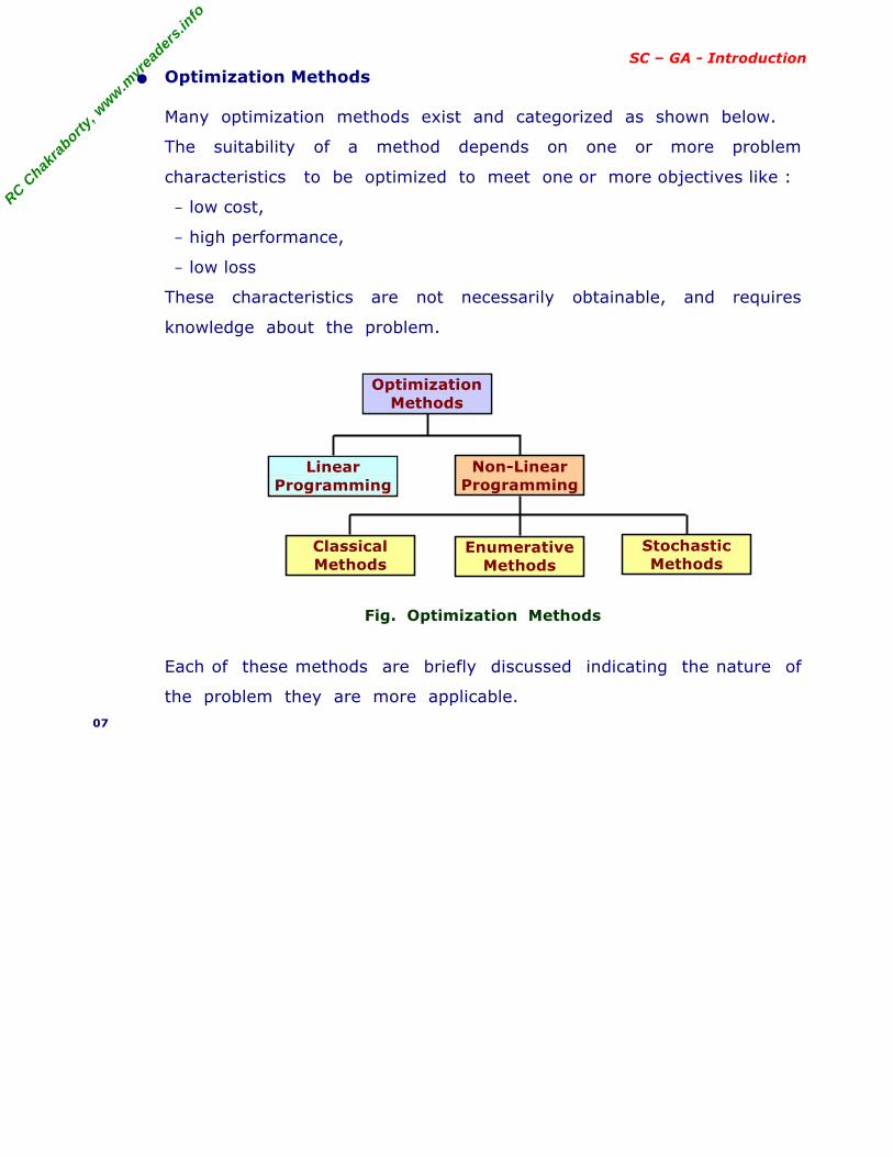
SC – GA - Introduction • Optimization Methods
Many optimization methods exist and categorized as shown below.
The suitability of a method depends on one or more problem
characteristics to be optimized to meet one or more objectives like :
− low cost,
− high performance,
− low loss
These characteristics are not necessarily obtainable, and requires
knowledge about the problem.
Fig. Optimization Methods
Each of these methods are briefly discussed indicating the nature of
the problem they are more applicable. 07
OptimizationMethods
Non-Linear Programming
Linear Programming
Stochastic Methods
Classical Methods
Enumerative Methods
RC C
hakra
borty,
ww
w.m
yrea
ders.
info
SC – GA - Introduction ■ Linear Programming
Intends to obtain the optimal solution to problems that are
perfectly represented by a set of linear equations; thus require
a priori knowledge of the problem. Here the
− the functions to be minimized or maximized, is called objective
functions,
− the set of linear equations are called restrictions.
− the optimal solution, is the one that minimizes (or maximizes)
the objective function.
Example : “Traveling salesman”, seeking a minimal traveling distance.
08

RC C
hakra
borty,
ww
w.m
yrea
ders.
info
SC – GA - Introduction ■ Non- Linear Programming
Intended for problems described by non-linear equations.
The methods are divided in three large groups:
Classical, Enumerative and Stochastic.
Classical search uses deterministic approach to find best solution.
These methods requires knowledge of gradients or higher order
derivatives. In many practical problems, some desired information
are not available, means deterministic algorithms are inappropriate.
The techniques are subdivide into:
− Direct methods, e.g. Newton or Fibonacci
− Indirect methods.
Enumerative search goes through every point (one point at a
time ) related to the function's domain space. At each point, all
possible solutions are generated and tested to find optimum
solution. It is easy to implement but usually require significant
computation. In the field of artificial intelligence, the enumerative
methods are subdivided into two categories:
− Uninformed methods, e.g. Mini-Max algorithm
− Informed methods, e.g. Alpha-Beta and A* ,
Stochastic search deliberately introduces randomness into the search
process. The injected randomness may provide the necessary impetus
to move away from a local solution when searching for a global
optimum. e.g., a gradient vector criterion for “smoothing” problems.
Stochastic methods offer robustness quality to optimization process.
Among the stochastic techniques, the most widely used are :
− Evolutionary Strategies (ES),
− Genetic Algorithms (GA), and
− Simulated Annealing (SA).
The ES and GA emulate nature’s evolutionary behavior, while SA is
based on the physical process of annealing a material. 09
RC C
hakra
borty,
ww
w.m
yrea
ders.
info
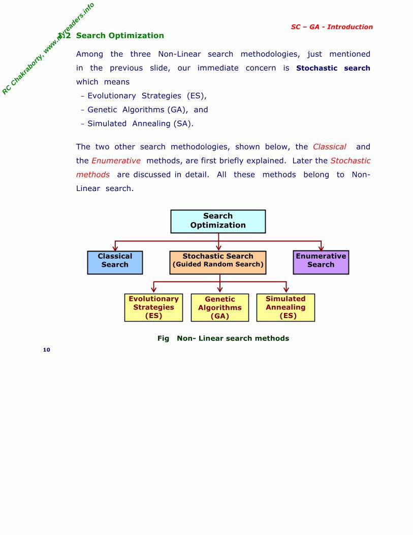
SC – GA - Introduction 1.2 Search Optimization
Among the three Non-Linear search methodologies, just mentioned
in the previous slide, our immediate concern is Stochastic search
which means
− Evolutionary Strategies (ES),
− Genetic Algorithms (GA), and
− Simulated Annealing (SA).
The two other search methodologies, shown below, the Classical and
the Enumerative methods, are first briefly explained. Later the Stochastic
methods are discussed in detail. All these methods belong to Non-
Linear search.
Fig Non- Linear search methods
10
Search Optimization
Stochastic Search (Guided Random Search)
Enumerative Search
Classical Search
Evolutionary Strategies
(ES)
Genetic Algorithms
(GA)
Simulated Annealing
(ES)
RC C
hakra
borty,
ww
w.m
yrea
ders.
info
SC – GA - Introduction • Classical or Calculus based search
Uses deterministic approach to find best solutions of an optimization
problem.
− the solutions satisfy a set of necessary and sufficient conditions of
the optimization problem.
− the techniques are subdivide into direct and indirect methods.
◊ Direct or Numerical methods :
− example : Newton or Fibonacci,
− tries to find extremes by "hopping" around the search space
and assessing the gradient of the new point, which
guides the search.
− applies the concept of "hill climbing", and finds the best
local point by climbing the steepest permissible gradient.
− used only on a restricted set of "well behaved" functions.
◊ Indirect methods :
− does search for local extremes by solving usually non-linear
set of equations resulting from setting the gradient of the
objective function to zero.
− does search for possible solutions (function peaks), starts by
restricting itself to points with zero slope in all directions.
11
RC C
hakra
borty,
ww
w.m
yrea
ders.
info
SC – GA - Introduction • Enumerative Search
Here the search goes through every point (one point at a time) related
to the function's domain space.
− At each point, all possible solutions are generated and tested to find
optimum solution.
− It is easy to implement but usually require significant computation.
Thus these techniques are not suitable for applications with large
domain spaces.
In the field of artificial intelligence, the enumerative methods are
subdivided into two categories : Uninformed and Informed methods.
◊ Uninformed or blind methods :
− example: Mini-Max algorithm,
− search all points in the space in a predefined order,
− used in game playing.
◊ Informed methods :
− example: Alpha-Beta and A* ,
− does more sophisticated search
− uses domain specific knowledge in the form of a cost
function or heuristic to reduce cost for search.
Next slide shows, the taxonomy of enumerative search in AI domain.
12
RC C
hakra
borty,
ww
w.m
yrea
ders.
info
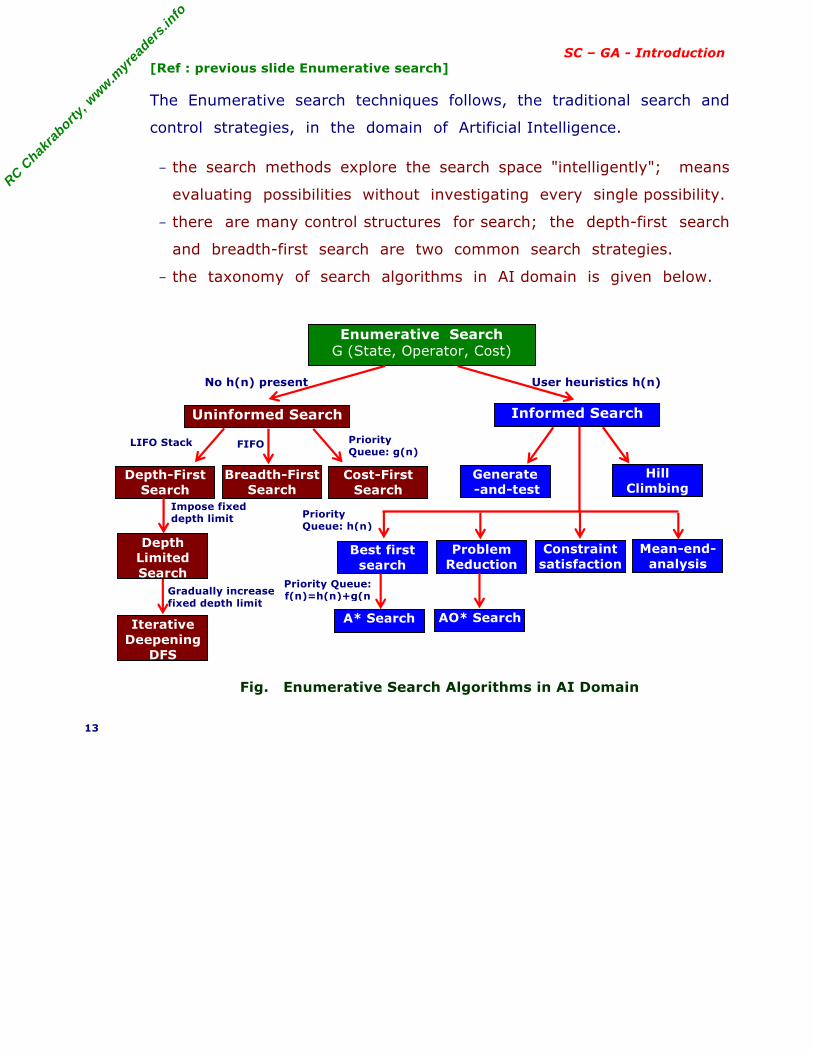
SC – GA - Introduction [Ref : previous slide Enumerative search]
The Enumerative search techniques follows, the traditional search and
control strategies, in the domain of Artificial Intelligence.
− the search methods explore the search space "intelligently"; means
evaluating possibilities without investigating every single possibility.
− there are many control structures for search; the depth-first search
and breadth-first search are two common search strategies.
− the taxonomy of search algorithms in AI domain is given below.
Fig. Enumerative Search Algorithms in AI Domain
13
User heuristics h(n)No h(n) present
Priority Queue:f(n)=h(n)+g(n
LIFO Stack
Gradually increase fixed depth limit
Impose fixed depth limit
Priority Queue: g(n)
Priority Queue: h(n)
FIFO
Enumerative Search G (State, Operator, Cost)
Informed Search Uninformed Search
Depth-First Search
Breadth-First Search
Cost-First Search
Generate -and-test
Hill Climbing
Depth Limited Search
Iterative Deepening
DFS
Problem Reduction
Constraint satisfaction
Mean-end-analysis
Best firstsearch
A* Search AO* Search
RC C
hakra
borty,
ww
w.m
yrea
ders.
info
SC – GA - Introduction • Stochastic Search
Here the search methods, include heuristics and an element of
randomness (non-determinism) in traversing the search space. Unlike
the previous two search methodologies
− the stochastic search algorithm moves from one point to another in
the search space in a non-deterministic manner, guided by heuristics.
− the stochastic search techniques are usually called Guided random
search techniques.
The stochastic search techniques are grouped into two major subclasses :
− Simulated annealing and
− Evolutionary algorithms.
Both these classes follow the principles of evolutionary processes.
◊ Simulated annealing (SAs)
− uses a thermodynamic evolution process to search
minimum energy states.
◊ Evolutionary algorithms (EAs)
− use natural selection principles.
− the search evolves throughout generations, improving the
features of potential solutions by means of biological
inspired operations.
− Genetic Algorithms (GAs) are a good example of this
technique.
The next slide shows, the taxonomy of evolutionary search algorithms.
It includes the other two search, the Enumerative search and Calculus
based techniques, for better understanding of Non-Linear search
methodologies in its entirety.
14
RC C
hakra
borty,
ww
w.m
yrea
ders.
info
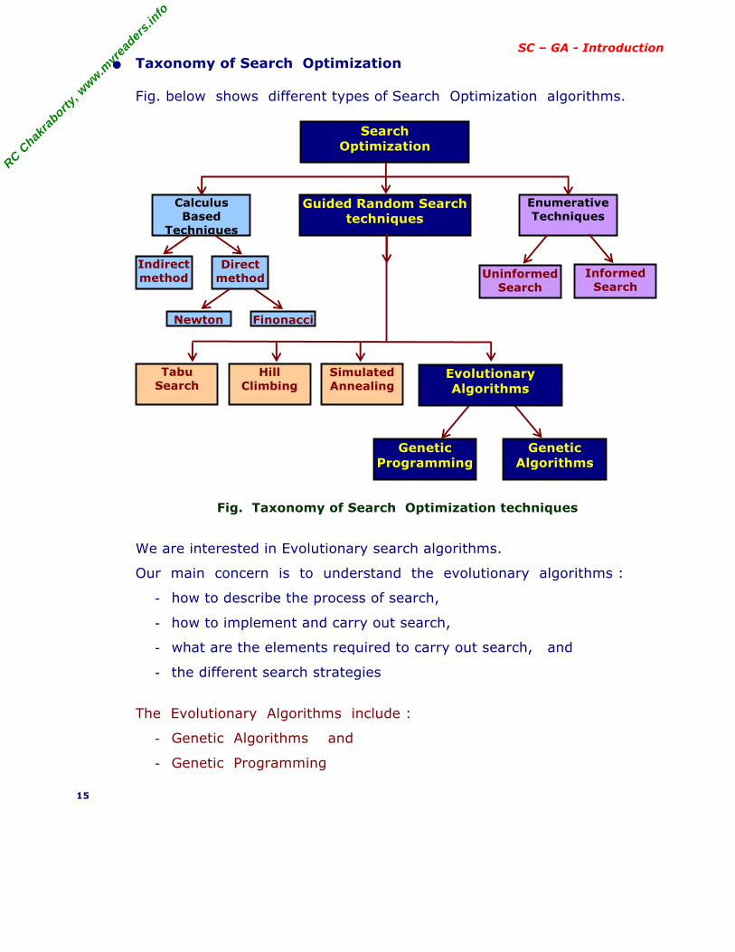
SC – GA - Introduction • Taxonomy of Search Optimization
Fig. below shows different types of Search Optimization algorithms.
Fig. Taxonomy of Search Optimization techniques
We are interested in Evolutionary search algorithms.
Our main concern is to understand the evolutionary algorithms :
- how to describe the process of search,
- how to implement and carry out search,
- what are the elements required to carry out search, and
- the different search strategies
The Evolutionary Algorithms include :
- Genetic Algorithms and
- Genetic Programming
15
Search Optimization
Guided Random Search techniques
Enumerative Techniques
Calculus Based
Techniques
Indirect method
Direct method
Simulated Annealing
Informed Search
Hill Climbing
Tabu Search
Genetic Algorithms
Genetic Programming
Newton Finonacci
Uninformed Search
Evolutionary Algorithms
RC C
hakra
borty,
ww
w.m
yrea
ders.
info
SC – GA - Introduction 1.3 Evolutionary Algorithm (EAs)
Evolutionary Algorithm (EA) is a subset of Evolutionary Computation (EC)
which is a subfield of Artificial Intelligence (AI).
Evolutionary Computation (EC) is a general term for several
computational techniques. Evolutionary Computation represents powerful
search and optimization paradigm influenced by biological mechanisms of
evolution : that of natural selection and genetic.
Evolutionary Algorithms (EAs) refers to Evolutionary Computational
models using randomness and genetic inspired operations. EAs
involve selection, recombination, random variation and competition of the
individuals in a population of adequately represented potential solutions.
The candidate solutions are referred as chromosomes or individuals.
Genetic Algorithms (GAs) represent the main paradigm of Evolutionary
Computation.
- GAs simulate natural evolution, mimicking processes the nature uses :
Selection, Crosses over, Mutation and Accepting.
- GAs simulate the survival of the fittest among individuals over
consecutive generation for solving a problem.
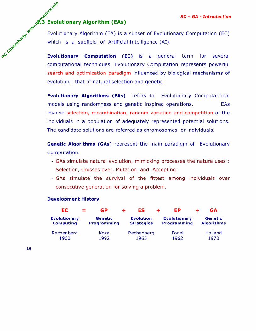
Development History
EC = GP + ES + EP + GA
Evolutionary Computing
Genetic Programming
Evolution Strategies
Evolutionary Programming
Genetic Algorithms
Rechenberg
1960 Koza
1992 Rechenberg
1965 Fogel
1962 Holland
1970
16
RC C
hakra
borty,
ww
w.m
yrea
ders.
info
SC – GA - Introduction 1.4 Genetic Algorithms (GAs) - Basic Concepts
Genetic algorithms (GAs) are the main paradigm of evolutionary
computing. GAs are inspired by Darwin's theory about evolution – the
"survival of the fittest". In nature, competition among individuals for
scanty resources results in the fittest individuals dominating over the
weaker ones.
− GAs are the ways of solving problems by mimicking processes nature
uses; ie., Selection, Crosses over, Mutation and Accepting, to evolve a
solution to a problem.
− GAs are adaptive heuristic search based on the evolutionary ideas
of natural selection and genetics.
− GAs are intelligent exploitation of random search used in optimization
problems.
− GAs, although randomized, exploit historical information to direct the
search into the region of better performance within the search space.
The biological background (basic genetics), the scheme of evolutionary
processes, the working principles and the steps involved in GAs are
illustrated in next few slides.
17
RC C
hakra
borty,
ww
w.m
yrea
ders.
info
SC – GA - Introduction • Biological Background – Basic Genetics
‡ Every organism has a set of rules, describing how that organism
is built. All living organisms consist of cells.
‡ In each cell there is same set of chromosomes. Chromosomes are
strings of DNA and serve as a model for the whole organism.
‡ A chromosome consists of genes, blocks of DNA.
‡ Each gene encodes a particular protein that represents a trait
(feature), e.g., color of eyes.
‡ Possible settings for a trait (e.g. blue, brown) are called alleles.
‡ Each gene has its own position in the chromosome called its locus.
‡ Complete set of genetic material (all chromosomes) is called a
genome.
‡ Particular set of genes in a genome is called genotype.
‡ The physical expression of the genotype (the organism itself after
birth) is called the phenotype, its physical and mental characteristics,
such as eye color, intelligence etc.
‡ When two organisms mate they share their genes; the resultant
offspring may end up having half the genes from one parent and half
from the other. This process is called recombination (cross over) .
‡ The new created offspring can then be mutated. Mutation means,
that the elements of DNA are a bit changed. This changes are mainly
caused by errors in copying genes from parents.
‡ The fitness of an organism is measured by success of the organism
in its life (survival).
18
RC C
hakra
borty,
ww
w.m
yrea
ders.
info
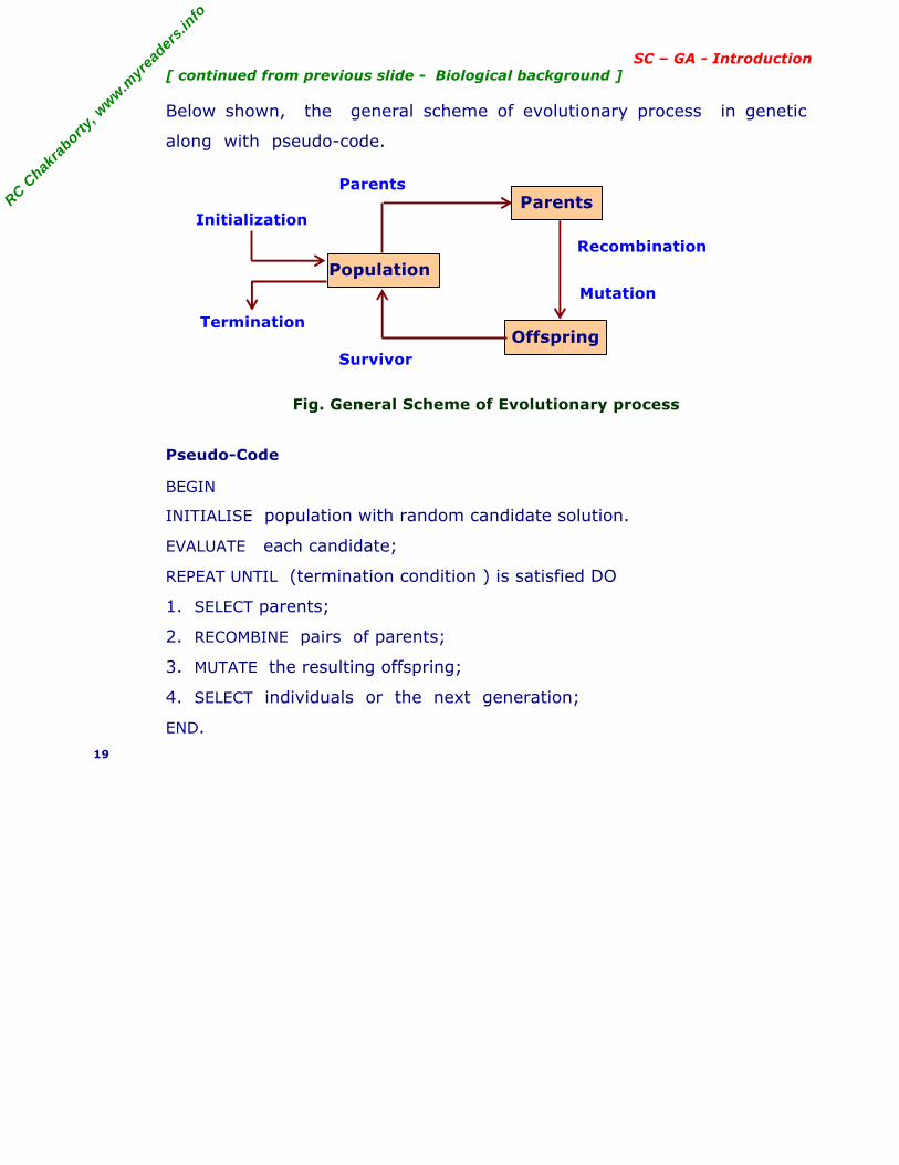
SC – GA - Introduction [ continued from previous slide - Biological background ]
Below shown, the general scheme of evolutionary process in genetic
along with pseudo-code.
Fig. General Scheme of Evolutionary process
Pseudo-Code
BEGIN
INITIALISE population with random candidate solution.
EVALUATE each candidate;
REPEAT UNTIL (termination condition ) is satisfied DO
1. SELECT parents;
2. RECOMBINE pairs of parents;
3. MUTATE the resulting offspring;
4. SELECT individuals or the next generation;
END. 19
Parents
Offspring
PopulationRecombination
Mutation
Parents
Termination
Initialization
Survivor
RC C
hakra
borty,
ww
w.m
yrea
ders.
info
SC – GA - Introduction • Search Space
In solving problems, some solution will be the best among others.
The space of all feasible solutions (among which the desired solution
resides) is called search space (also called state space).
− Each point in the search space represents one possible solution.
− Each possible solution can be "marked" by its value (or fitness) for
the problem.
− The GA looks for the best solution among a number of possible
solutions represented by one point in the search space.
− Looking for a solution is then equal to looking for some extreme value
(minimum or maximum) in the search space.
− At times the search space may be well defined, but usually only a few
points in the search space are known.
In using GA, the process of finding solutions generates other points
(possible solutions) as evolution proceeds.
20
RC C
hakra
borty,
ww
w.m
yrea
ders.
info
SC – GA - Introduction • Working Principles
Before getting into GAs, it is necessary to explain few terms.
− Chromosome : a set of genes; a chromosome contains the solution in
form of genes.
− Gene : a part of chromosome; a gene contains a part of solution. It
determines the solution. e.g. 16743 is a chromosome and 1, 6, 7, 4
and 3 are its genes.
− Individual : same as chromosome.
− Population: number of individuals present with same length of
chromosome.
− Fitness : the value assigned to an individual based on how far or
close a individual is from the solution; greater the fitness value better
the solution it contains.
− Fitness function : a function that assigns fitness value to the individual.
It is problem specific.
− Breeding : taking two fit individuals and then intermingling there
chromosome to create new two individuals.
− Mutation : changing a random gene in an individual.
− Selection : selecting individuals for creating the next generation.
Working principles :
Genetic algorithm begins with a set of solutions (represented by
chromosomes) called the population.
− Solutions from one population are taken and used to form a new
population. This is motivated by the possibility that the new population
will be better than the old one.
− Solutions are selected according to their fitness to form new solutions
(offspring); more suitable they are, more chances they have to
reproduce.
− This is repeated until some condition (e.g. number of populations or
improvement of the best solution) is satisfied.
21
RC C
hakra
borty,
ww
w.m
yrea
ders.
info
SC – GA - Introduction • Outline of the Basic Genetic Algorithm
1. [Start] Generate random population of n chromosomes (i.e. suitable
solutions for the problem). 2. [Fitness] Evaluate the fitness f(x) of each chromosome x in the
population. 3. [New population] Create a new population by repeating following
steps until the new population is complete. (a) [Selection] Select two parent chromosomes from a population
according to their fitness (better the fitness, bigger the chance to
be selected) (b) [Crossover] With a crossover probability, cross over the parents
to form new offspring (children). If no crossover was performed,
offspring is the exact copy of parents. (c) [Mutation] With a mutation probability, mutate new offspring at
each locus (position in chromosome). (d) [Accepting] Place new offspring in the new population 4. [Replace] Use new generated population for a further run of the
algorithm 5. [Test] If the end condition is satisfied, stop, and return the best
solution in current population 6. [Loop] Go to step 2
Note : The genetic algorithm's performance is largely influenced by two
operators called crossover and mutation. These two operators are the
most important parts of GA. 22
RC C
hakra
borty,
ww
w.m
yrea
ders.
info
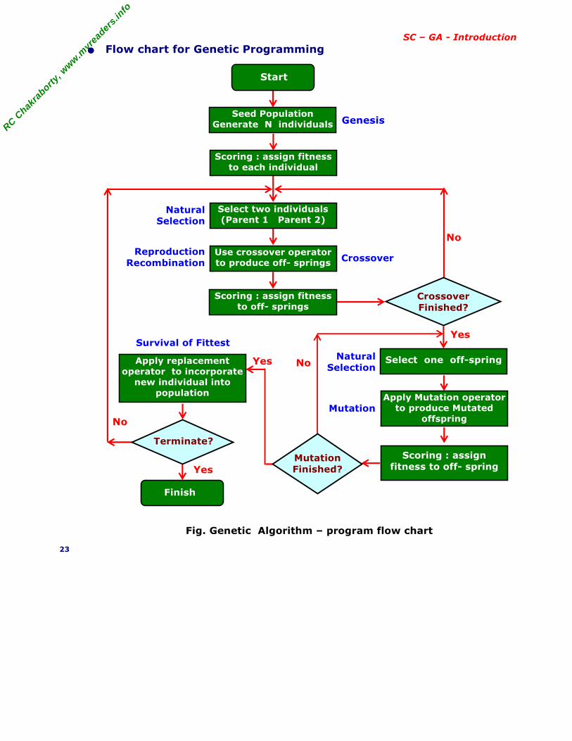
SC – GA - Introduction • Flow chart for Genetic Programming
Fig. Genetic Algorithm – program flow chart
23
Yes
No
No
NoNatural
Selection
Natural Selection
Mutation
Crossover
Survival of Fittest
Reproduction Recombination
Genesis
Yes
Yes
Seed PopulationGenerate N individuals
Scoring : assign fitness to each individual
Select two individuals(Parent 1 Parent 2)
Select one off-spring
Use crossover operator to produce off- springs
Scoring : assign fitness to off- springs
Apply replacement operator to incorporate
new individual into population
MutationFinished?
Terminate?
Finish
CrossoverFinished?
Start
Apply Mutation operator to produce Mutated
offspring
Scoring : assign fitness to off- spring
RC C
hakra
borty,
ww
w.m
yrea
ders.
info
SC – GA - Encoding 2. Encoding
Before a genetic algorithm can be put to work on any problem, a method is
needed to encode potential solutions to that problem in a form so that a
computer can process.
− One common approach is to encode solutions as binary strings: sequences
of 1's and 0's, where the digit at each position represents the value of
some aspect of the solution.
Example :
A Gene represents some data (eye color, hair color, sight, etc.).
A chromosome is an array of genes. In binary form
a Gene looks like : (11100010)
a Chromosome looks like: Gene1 Gene2 Gene3 Gene4
(11000010, 00001110, 001111010, 10100011)
A chromosome should in some way contain information about solution
which it represents; it thus requires encoding. The most popular way of
encoding is a binary string like :
Chromosome 1 : 1101100100110110
Chromosome 2 : 1101111000011110
Each bit in the string represent some characteristics of the solution.
− There are many other ways of encoding, e.g., encoding values as integer or
real numbers or some permutations and so on.
− The virtue of these encoding method depends on the problem to work on .
24
RC C
hakra
borty,
ww
w.m
yrea
ders.
info
SC – GA - Encoding • Binary Encoding
Binary encoding is the most common to represent information contained.
In genetic algorithms, it was first used because of its relative simplicity.
− In binary encoding, every chromosome is a string of bits : 0 or 1, like
Chromosome 1: 1 0 1 1 0 0 1 0 1 1 0 0 1 0 1 0 1 1 1 0 0 1 0 1
Chromosome 2: 1 1 1 1 1 1 1 0 0 0 0 0 1 1 0 0 0 0 0 1 1 1 1 1
− Binary encoding gives many possible chromosomes even with a small
number of alleles ie possible settings for a trait (features).
− This encoding is often not natural for many problems and sometimes
corrections must be made after crossover and/or mutation.
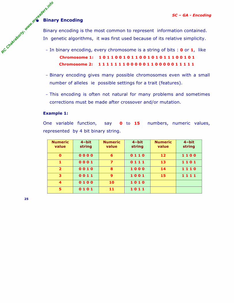
Example 1:
One variable function, say 0 to 15 numbers, numeric values,
represented by 4 bit binary string.
Numeric value
4–bit string
Numeric value
4–bit string
Numeric value
4–bit string
0 0 0 0 0 6 0 1 1 0 12 1 1 0 0
1 0 0 0 1 7 0 1 1 1 13 1 1 0 1
2 0 0 1 0 8 1 0 0 0 14 1 1 1 0
3 0 0 1 1 9 1 0 0 1 15 1 1 1 1
4 0 1 0 0 10 1 0 1 0
5 0 1 0 1 11 1 0 1 1
25
RC C
hakra
borty,
ww
w.m
yrea
ders.
info
SC – GA - Encoding [ continued binary encoding ]
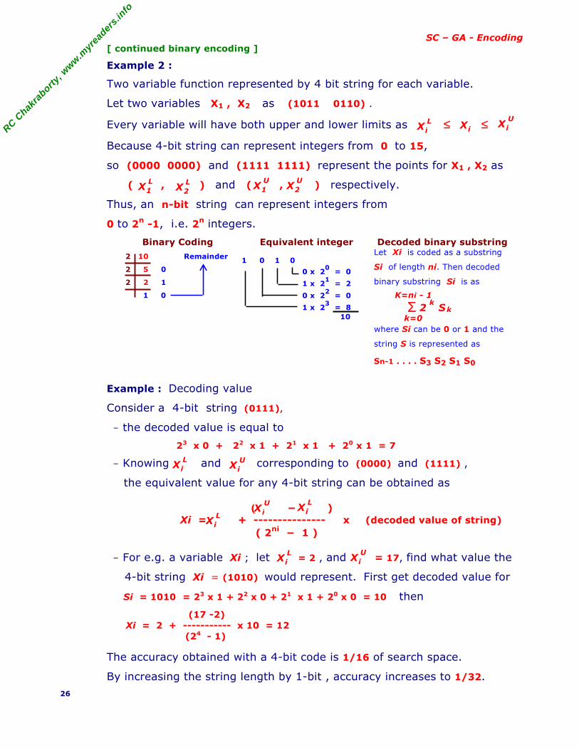
Example 2 :
Two variable function represented by 4 bit string for each variable.
Let two variables X1 , X2 as (1011 0110) .
Every variable will have both upper and lower limits as ≤ ≤
Because 4-bit string can represent integers from 0 to 15,
so (0000 0000) and (1111 1111) represent the points for X1 , X2 as
( , ) and ( , ) respectively.
Thus, an n-bit string can represent integers from
0 to 2n -1, i.e. 2n integers.
Binary Coding Equivalent integer Decoded binary substring
1 0 1 0
0 x 20 = 0
1 x 21 = 2
0 x 22 = 0
1 x 23 = 8
10
Let Xi is coded as a substring
Si of length ni. Then decoded
binary substring Si is as
where Si can be 0 or 1 and the
string S is represented as
Sn-1 . . . . S3 S2 S1 S0
Example : Decoding value
Consider a 4-bit string (0111),
− the decoded value is equal to
23 x 0 + 22 x 1 + 21 x 1 + 20 x 1 = 7
− Knowing and corresponding to (0000) and (1111) ,
the equivalent value for any 4-bit string can be obtained as
( − ) Xi = + --------------- x (decoded value of string) ( 2ni − 1 )
− For e.g. a variable Xi ; let = 2 , and = 17, find what value the
4-bit string Xi = (1010) would represent. First get decoded value for
Si = 1010 = 23 x 1 + 22 x 0 + 21 x 1 + 20 x 0 = 10 then
(17 -2) Xi = 2 + ----------- x 10 = 12
(24 - 1)
The accuracy obtained with a 4-bit code is 1/16 of search space.
By increasing the string length by 1-bit , accuracy increases to 1/32. 26
X L i
Xi XUi
X L 1 X
L 2
XU2X
U1
2 10 Remainder
2 5 0
2 2 1
1 0
Σ k=0
K=ni - 1
2 k S
k
X L i X
Ui
X L i
XUi X
Li
XLi X
Ui
RC C
hakra
borty,
ww
w.m
yrea
ders.
info
SC – GA - Encoding • Value Encoding
The Value encoding can be used in problems where values such as real
numbers are used. Use of binary encoding for this type of problems
would be difficult.
1. In value encoding, every chromosome is a sequence of some values.
2. The Values can be anything connected to the problem, such as :
real numbers, characters or objects.
Examples :
Chromosome A 1.2324 5.3243 0.4556 2.3293 2.4545
Chromosome B ABDJEIFJDHDIERJFDLDFLFEGT
Chromosome C (back), (back), (right), (forward), (left)
3. Value encoding is often necessary to develop some new types of
crossovers and mutations specific for the problem.
27
RC C
hakra
borty,
ww
w.m
yrea
ders.
info
SC – GA - Encoding • Permutation Encoding
Permutation encoding can be used in ordering problems, such as traveling
salesman problem or task ordering problem.
1. In permutation encoding, every chromosome is a string of numbers
that represent a position in a sequence.
Chromosome A 1 5 3 2 6 4 7 9 8
Chromosome B 8 5 6 7 2 3 1 4 9
2. Permutation encoding is useful for ordering problems. For some
problems, crossover and mutation corrections must be made to
leave the chromosome consistent.
Examples :
1. The Traveling Salesman problem:
There are cities and given distances between them. Traveling
salesman has to visit all of them, but he does not want to travel more
than necessary. Find a sequence of cities with a minimal traveled
distance. Here, encoded chromosomes describe the order of cities the
salesman visits.
2. The Eight Queens problem :
There are eight queens. Find a way to place them on a chess board
so that no two queens attack each other. Here, encoding
describes the position of a queen on each row.
28
RC C
hakra
borty,
ww
w.m
yrea
ders.
info
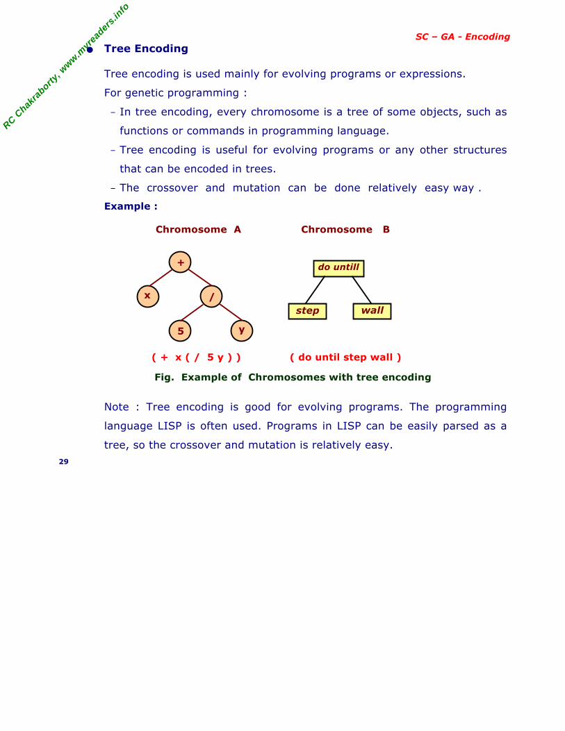
SC – GA - Encoding • Tree Encoding
Tree encoding is used mainly for evolving programs or expressions.
For genetic programming :
− In tree encoding, every chromosome is a tree of some objects, such as
functions or commands in programming language.
− Tree encoding is useful for evolving programs or any other structures
that can be encoded in trees.
− The crossover and mutation can be done relatively easy way .
Example :
Chromosome A
Chromosome B
( + x ( / 5 y ) ) ( do until step wall )
Fig. Example of Chromosomes with tree encoding
Note : Tree encoding is good for evolving programs. The programming
language LISP is often used. Programs in LISP can be easily parsed as a
tree, so the crossover and mutation is relatively easy. 29
+
/ x
y5
do untill
step wall
RC C
hakra
borty,
ww
w.m
yrea
ders.
info
SC – GA - Operators 3. Operators of Genetic Algorithm
Genetic operators used in genetic algorithms maintain genetic diversity.
Genetic diversity or variation is a necessity for the process of evolution.
Genetic operators are analogous to those which occur in the natural world:
− Reproduction (or Selection) ;
− Crossover (or Recombination); and
− Mutation.
In addition to these operators, there are some parameters of GA.
One important parameter is Population size.
− Population size says how many chromosomes are in population (in one
generation).
− If there are only few chromosomes, then GA would have a few possibilities
to perform crossover and only a small part of search space is explored.
− If there are many chromosomes, then GA slows down.
− Research shows that after some limit, it is not useful to increase population
size, because it does not help in solving the problem faster. The population
size depends on the type of encoding and the problem.
30
RC C
hakra
borty,
ww
w.m
yrea
ders.
info
SC – GA - Operators 3.1 Reproduction, or Selection
Reproduction is usually the first operator applied on population. From
the population, the chromosomes are selected to be parents to crossover
and produce offspring.
The problem is how to select these chromosomes ?
According to Darwin's evolution theory "survival of the fittest" – the best
ones should survive and create new offspring.
− The Reproduction operators are also called Selection operators.
− Selection means extract a subset of genes from an existing population,
according to any definition of quality. Every gene has a meaning, so
one can derive from the gene a kind of quality measurement called
fitness function. Following this quality (fitness value), selection can be
performed.
− Fitness function quantifies the optimality of a solution (chromosome) so
that a particular solution may be ranked against all the other solutions.
The function depicts the closeness of a given ‘solution’ to the desired
result.
Many reproduction operators exists and they all essentially do same thing.
They pick from current population the strings of above average and insert
their multiple copies in the mating pool in a probabilistic manner.
The most commonly used methods of selecting chromosomes for parents
to crossover are :
− Roulette wheel selection, − Rank selection
− Boltzmann selection, − Steady state selection.
− Tournament selection,
The Roulette wheel and Boltzmann selections methods are illustrated next.31
RC C
hakra
borty,
ww
w.m
yrea
ders.
info
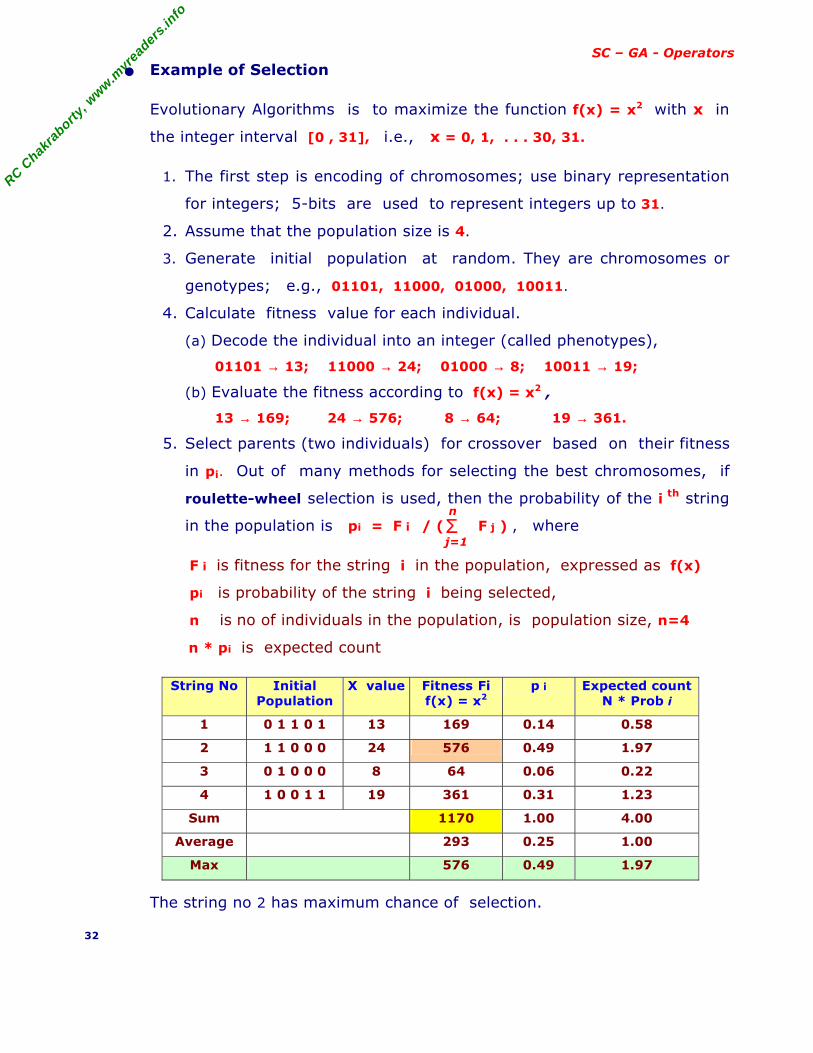
SC – GA - Operators • Example of Selection
Evolutionary Algorithms is to maximize the function f(x) = x2 with x in
the integer interval [0 , 31], i.e., x = 0, 1, . . . 30, 31.
1. The first step is encoding of chromosomes; use binary representation
for integers; 5-bits are used to represent integers up to 31.
2. Assume that the population size is 4.
3. Generate initial population at random. They are chromosomes or
genotypes; e.g., 01101, 11000, 01000, 10011.
4. Calculate fitness value for each individual.
(a) Decode the individual into an integer (called phenotypes),
01101 → 13; 11000 → 24; 01000 → 8; 10011 → 19;
(b) Evaluate the fitness according to f(x) = x2 ,
13 → 169; 24 → 576; 8 → 64; 19 → 361.
5. Select parents (two individuals) for crossover based on their fitness
in pi. Out of many methods for selecting the best chromosomes, if
roulette-wheel selection is used, then the probability of the i th string
in the population is pi = F i / ( F j ) , where
F i is fitness for the string i in the population, expressed as f(x)
pi is probability of the string i being selected,
n is no of individuals in the population, is population size, n=4
n * pi is expected count
String No Initial Population
X value Fitness Fi f(x) = x2
p i Expected countN * Prob i
1 0 1 1 0 1 13 169 0.14 0.58
2 1 1 0 0 0 24 576 0.49 1.97
3 0 1 0 0 0 8 64 0.06 0.22
4 1 0 0 1 1 19 361 0.31 1.23
Sum 1170 1.00 4.00
Average 293 0.25 1.00
Max 576 0.49 1.97
The string no 2 has maximum chance of selection.
32
Σj=1
n
RC C
hakra
borty,
ww
w.m
yrea
ders.
info
SC – GA - Operators • Roulette wheel selection (Fitness-Proportionate Selection)
Roulette-wheel selection, also known as Fitness Proportionate Selection, is
a genetic operator, used for selecting potentially useful solutions for
recombination.
In fitness-proportionate selection :
− the chance of an individual's being selected is proportional to its
fitness, greater or less than its competitors' fitness.
− conceptually, this can be thought as a game of Roulette.
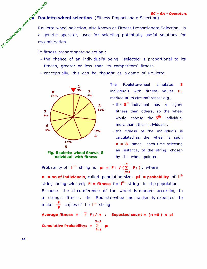
Fig. Roulette-wheel Shows 8 individual with fitness
The Roulette-wheel simulates 8
individuals with fitness values Fi,
marked at its circumference; e.g.,
− the 5th individual has a higher
fitness than others, so the wheel
would choose the 5th individual
more than other individuals .
− the fitness of the individuals is
calculated as the wheel is spun
n = 8 times, each time selecting
an instance, of the string, chosen
by the wheel pointer.
Probability of i th string is pi = F i / ( F j ) , where
n = no of individuals, called population size; pi = probability of ith
string being selected; Fi = fitness for ith string in the population.
Because the circumference of the wheel is marked according to
a string's fitness, the Roulette-wheel mechanism is expected to
make copies of the ith string.
Average fitness = F j / n ; Expected count = (n =8 ) x pi
Cumulative Probability5 = pi
33
5% 1
9%2
13%3
17%
4
8% 6
8% 7
20% 8
20% 5
Σj=1
n
F
F
F
Σi=1
N=5
RC C
hakra
borty,
ww
w.m
yrea
ders.
info
SC – GA - Operators • Boltzmann Selection
Simulated annealing is a method used to minimize or maximize a function.
− This method simulates the process of slow cooling of molten metal to
achieve the minimum function value in a minimization problem.
− The cooling phenomena is simulated by controlling a temperature like
parameter introduced with the concept of Boltzmann probability
distribution.
− The system in thermal equilibrium at a temperature T has its energy
distribution based on the probability defined by
P(E) = exp ( - E / kT ) were k is Boltzmann constant.
− This expression suggests that a system at a higher temperature has
almost uniform probability at any energy state, but at lower
temperature it has a small probability of being at a higher energy state.
− Thus, by controlling the temperature T and assuming that the search
process follows Boltzmann probability distribution, the convergence of
the algorithm is controlled.
34
RC C
hakra
borty,
ww
w.m
yrea
ders.
info
SC – GA - Operators 3.2 Crossover
Crossover is a genetic operator that combines (mates) two chromosomes
(parents) to produce a new chromosome (offspring). The idea behind
crossover is that the new chromosome may be better than both of the
parents if it takes the best characteristics from each of the parents.
Crossover occurs during evolution according to a user-definable crossover
probability. Crossover selects genes from parent chromosomes and
creates a new offspring.
The Crossover operators are of many types.
− one simple way is, One-Point crossover.
− the others are Two Point, Uniform, Arithmetic, and Heuristic crossovers.
The operators are selected based on the way chromosomes are encoded.
35
RC C
hakra
borty,
ww
w.m
yrea
ders.
info
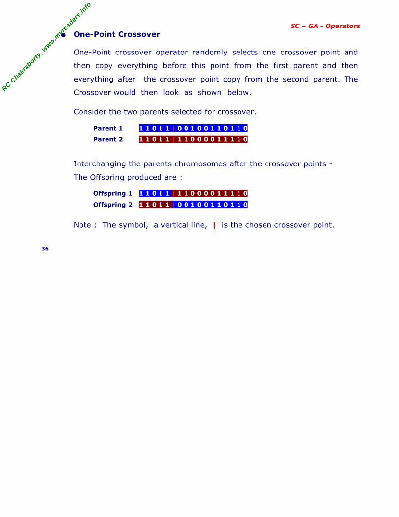
SC – GA - Operators • One-Point Crossover
One-Point crossover operator randomly selects one crossover point and
then copy everything before this point from the first parent and then
everything after the crossover point copy from the second parent. The
Crossover would then look as shown below.
Consider the two parents selected for crossover.
Parent 1 1 1 0 1 1 | 0 0 1 0 0 1 1 0 1 1 0
Parent 2 1 1 0 1 1 | 1 1 0 0 0 0 1 1 1 1 0
Interchanging the parents chromosomes after the crossover points -
The Offspring produced are :
Offspring 1 1 1 0 1 1 | 1 1 0 0 0 0 1 1 1 1 0
Offspring 2 1 1 0 1 1 | 0 0 1 0 0 1 1 0 1 1 0
Note : The symbol, a vertical line, | is the chosen crossover point.
36
RC C
hakra
borty,
ww
w.m
yrea
ders.
info
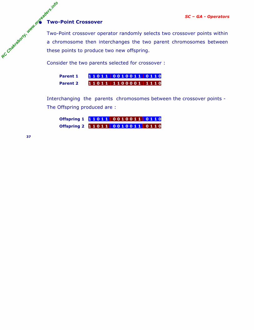
SC – GA - Operators • Two-Point Crossover
Two-Point crossover operator randomly selects two crossover points within
a chromosome then interchanges the two parent chromosomes between
these points to produce two new offspring.
Consider the two parents selected for crossover :
Parent 1 1 1 0 1 1 | 0 0 1 0 0 1 1 | 0 1 1 0
Parent 2 1 1 0 1 1 | 1 1 0 0 0 0 1 | 1 1 1 0
Interchanging the parents chromosomes between the crossover points -
The Offspring produced are :
Offspring 1 1 1 0 1 1 | 0 0 1 0 0 1 1 | 0 1 1 0
Offspring 2 1 1 0 1 1 | 0 0 1 0 0 1 1 | 0 1 1 0
37
RC C
hakra
borty,
ww
w.m
yrea
ders.
info
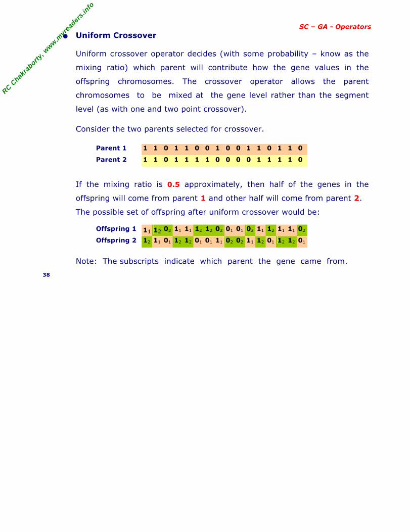
SC – GA - Operators • Uniform Crossover
Uniform crossover operator decides (with some probability – know as the
mixing ratio) which parent will contribute how the gene values in the
offspring chromosomes. The crossover operator allows the parent
chromosomes to be mixed at the gene level rather than the segment
level (as with one and two point crossover).
Consider the two parents selected for crossover.
Parent 1 1 1 0 1 1 0 0 1 0 0 1 1 0 1 1 0
Parent 2 1 1 0 1 1 1 1 0 0 0 0 1 1 1 1 0
If the mixing ratio is 0.5 approximately, then half of the genes in the
offspring will come from parent 1 and other half will come from parent 2.
The possible set of offspring after uniform crossover would be:
Offspring 1 11 12 02 11 11 12 12 02 01 01 02 11 12 11 11 02
Offspring 2 12 11 01 12 12 01 01 11 02 02 11 12 01 12 12 01
Note: The subscripts indicate which parent the gene came from.
38
RC C
hakra
borty,
ww
w.m
yrea
ders.
info
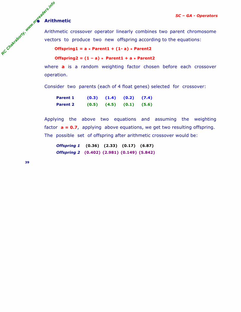
SC – GA - Operators • Arithmetic
Arithmetic crossover operator linearly combines two parent chromosome
vectors to produce two new offspring according to the equations:
Offspring1 = a * Parent1 + (1- a) * Parent2
Offspring2 = (1 – a) * Parent1 + a * Parent2
where a is a random weighting factor chosen before each crossover
operation.
Consider two parents (each of 4 float genes) selected for crossover:
Parent 1 (0.3) (1.4) (0.2) (7.4)
Parent 2 (0.5) (4.5) (0.1) (5.6)
Applying the above two equations and assuming the weighting
factor a = 0.7, applying above equations, we get two resulting offspring.
The possible set of offspring after arithmetic crossover would be:
Offspring 1 (0.36) (2.33) (0.17) (6.87)
Offspring 2 (0.402) (2.981) (0.149) (5.842)
39
RC C
hakra
borty,
ww
w.m
yrea
ders.
info
SC – GA - Operators • Heuristic
Heuristic crossover operator uses the fitness values of the two parent
chromosomes to determine the direction of the search.
The offspring are created according to the equations:
Offspring1 = BestParent + r * (BestParent − WorstParent)
Offspring2 = BestParent
where r is a random number between 0 and 1.
It is possible that offspring1 will not be feasible. It can happen if r is
chosen such that one or more of its genes fall outside of the allowable
upper or lower bounds. For this reason, heuristic crossover has a user
defined parameter n for the number of times to try and find an r
that results in a feasible chromosome. If a feasible chromosome is not
produced after n tries, the worst parent is returned as offspring1.
40
RC C
hakra
borty,
ww
w.m
yrea
ders.
info
SC – GA - Operators 3.3 Mutation
After a crossover is performed, mutation takes place.
Mutation is a genetic operator used to maintain genetic diversity from
one generation of a population of chromosomes to the next.
Mutation occurs during evolution according to a user-definable mutation
probability, usually set to fairly low value, say 0.01 a good first choice.
Mutation alters one or more gene values in a chromosome from its initial
state. This can result in entirely new gene values being added to the
gene pool. With the new gene values, the genetic algorithm may be able
to arrive at better solution than was previously possible.
Mutation is an important part of the genetic search, helps to prevent the
population from stagnating at any local optima. Mutation is intended to
prevent the search falling into a local optimum of the state space.
The Mutation operators are of many type.
− one simple way is, Flip Bit.
− the others are Boundary, Non-Uniform, Uniform, and Gaussian.
The operators are selected based on the way chromosomes are
encoded .
41
RC C
hakra
borty,
ww
w.m
yrea
ders.
info
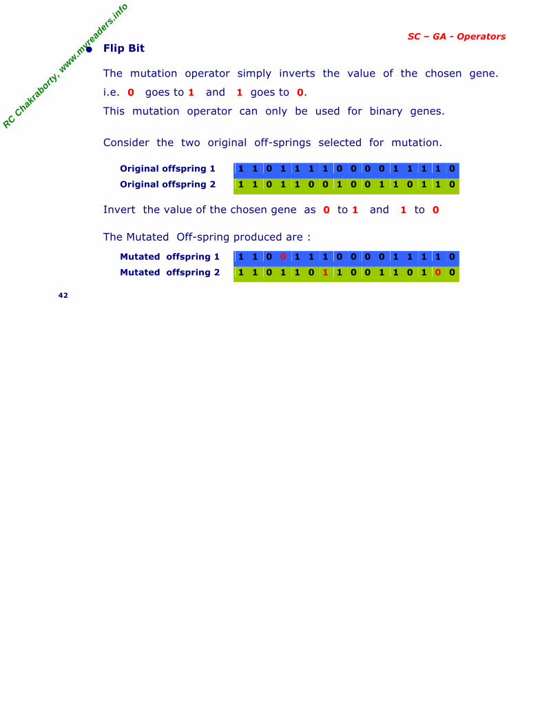
SC – GA - Operators • Flip Bit
The mutation operator simply inverts the value of the chosen gene.
i.e. 0 goes to 1 and 1 goes to 0.
This mutation operator can only be used for binary genes.
Consider the two original off-springs selected for mutation.
Original offspring 1 1 1 0 1 1 1 1 0 0 0 0 1 1 1 1 0
Original offspring 2 1 1 0 1 1 0 0 1 0 0 1 1 0 1 1 0
Invert the value of the chosen gene as 0 to 1 and 1 to 0
The Mutated Off-spring produced are :
Mutated offspring 1 1 1 0 0 1 1 1 0 0 0 0 1 1 1 1 0
Mutated offspring 2 1 1 0 1 1 0 1 1 0 0 1 1 0 1 0 0
42
RC C
hakra
borty,
ww
w.m
yrea
ders.
info
SC – GA - Operators • Boundary
The mutation operator replaces the value of the chosen gene with either
the upper or lower bound for that gene (chosen randomly).
This mutation operator can only be used for integer and float genes.
• Non-Uniform
The mutation operator increases the probability such that the amount of
the mutation will be close to 0 as the generation number increases. This
mutation operator prevents the population from stagnating in the early
stages of the evolution then allows the genetic algorithm to fine tune the
solution in the later stages of evolution.
This mutation operator can only be used for integer and float genes.
• Uniform
The mutation operator replaces the value of the chosen gene with a
uniform random value selected between the user-specified upper and
lower bounds for that gene.
This mutation operator can only be used for integer and float genes.
• Gaussian
The mutation operator adds a unit Gaussian distributed random value to
the chosen gene. The new gene value is clipped if it falls outside of the
user-specified lower or upper bounds for that gene.
This mutation operator can only be used for integer and float genes.
43
RC C
hakra
borty,
ww
w.m
yrea
ders.
info
SC – GA - Examples 4. Basic Genetic Algorithm :
Examples to demonstrate and explain : Random population, Fitness, Selection,
Crossover, Mutation, and Accepting.
• Example 1 :
Maximize the function f(x) = x2 over the range of integers from 0 . . . 31.
Note : This function could be solved by a variety of traditional methods
such as a hill-climbing algorithm which uses the derivative.
One way is to :
− Start from any integer x in the domain of f
− Evaluate at this point x the derivative f’
− Observing that the derivative is +ve, pick a new x which is at a small
distance in the +ve direction from current x
− Repeat until x = 31
See, how a genetic algorithm would approach this problem ?
44
RC C
hakra
borty,
ww
w.m
yrea
ders.
info
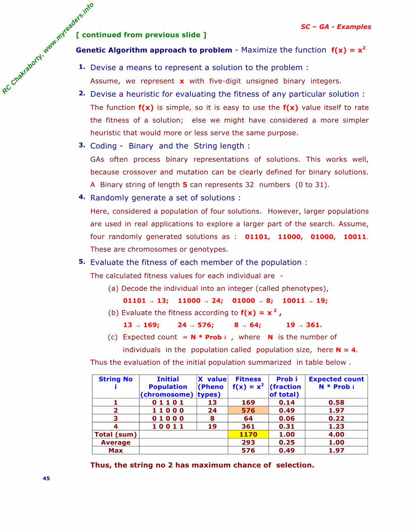
SC – GA - Examples [ continued from previous slide ]
Genetic Algorithm approach to problem - Maximize the function f(x) = x2
1. Devise a means to represent a solution to the problem :
Assume, we represent x with five-digit unsigned binary integers.
2. Devise a heuristic for evaluating the fitness of any particular solution :
The function f(x) is simple, so it is easy to use the f(x) value itself to rate
the fitness of a solution; else we might have considered a more simpler
heuristic that would more or less serve the same purpose.
3. Coding - Binary and the String length :
GAs often process binary representations of solutions. This works well,
because crossover and mutation can be clearly defined for binary solutions.
A Binary string of length 5 can represents 32 numbers (0 to 31).
4. Randomly generate a set of solutions :
Here, considered a population of four solutions. However, larger populations
are used in real applications to explore a larger part of the search. Assume,
four randomly generated solutions as : 01101, 11000, 01000, 10011.
These are chromosomes or genotypes.
5. Evaluate the fitness of each member of the population :
The calculated fitness values for each individual are -
(a) Decode the individual into an integer (called phenotypes),
01101 → 13; 11000 → 24; 01000 → 8; 10011 → 19;
(b) Evaluate the fitness according to f(x) = x 2 ,
13 → 169; 24 → 576; 8 → 64; 19 → 361.
(c) Expected count = N * Prob i , where N is the number of
individuals in the population called population size, here N = 4.
Thus the evaluation of the initial population summarized in table below .
String No i
Initial Population
(chromosome)
X value(Pheno types)
Fitness f(x) = x2
Prob i (fraction of total)
Expected countN * Prob i
1 0 1 1 0 1 13 169 0.14 0.58 2 1 1 0 0 0 24 576 0.49 1.97 3 0 1 0 0 0 8 64 0.06 0.22 4 1 0 0 1 1 19 361 0.31 1.23
Total (sum) 1170 1.00 4.00 Average 293 0.25 1.00
Max 576 0.49 1.97
Thus, the string no 2 has maximum chance of selection.
45
RC C
hakra
borty,
ww
w.m
yrea
ders.
info
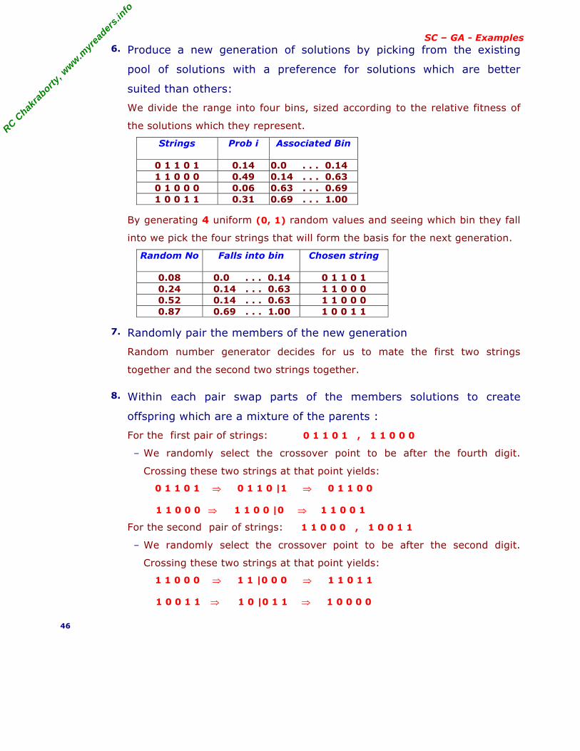
SC – GA - Examples 6. Produce a new generation of solutions by picking from the existing
pool of solutions with a preference for solutions which are better
suited than others:
We divide the range into four bins, sized according to the relative fitness of
the solutions which they represent.
Strings
Prob i
Associated Bin
0 1 1 0 1 0.14 0.0 . . . 0.14 1 1 0 0 0 0.49 0.14 . . . 0.63 0 1 0 0 0 0.06 0.63 . . . 0.69 1 0 0 1 1 0.31 0.69 . . . 1.00
By generating 4 uniform (0, 1) random values and seeing which bin they fall
into we pick the four strings that will form the basis for the next generation.
Random No Falls into bin
Chosen string
0.08 0.0 . . . 0.14 0 1 1 0 1 0.24 0.14 . . . 0.63 1 1 0 0 0 0.52 0.14 . . . 0.63 1 1 0 0 0 0.87 0.69 . . . 1.00 1 0 0 1 1
7. Randomly pair the members of the new generation
Random number generator decides for us to mate the first two strings
together and the second two strings together.
8. Within each pair swap parts of the members solutions to create
offspring which are a mixture of the parents :
For the first pair of strings: 0 1 1 0 1 , 1 1 0 0 0
− We randomly select the crossover point to be after the fourth digit.
Crossing these two strings at that point yields:
0 1 1 0 1 ⇒ 0 1 1 0 |1 ⇒ 0 1 1 0 0 1 1 0 0 0 ⇒ 1 1 0 0 |0 ⇒ 1 1 0 0 1
For the second pair of strings: 1 1 0 0 0 , 1 0 0 1 1
− We randomly select the crossover point to be after the second digit.
Crossing these two strings at that point yields:
1 1 0 0 0 ⇒ 1 1 |0 0 0 ⇒ 1 1 0 1 1 1 0 0 1 1 ⇒ 1 0 |0 1 1 ⇒ 1 0 0 0 0
46
RC C
hakra
borty,
ww
w.m
yrea
ders.
info
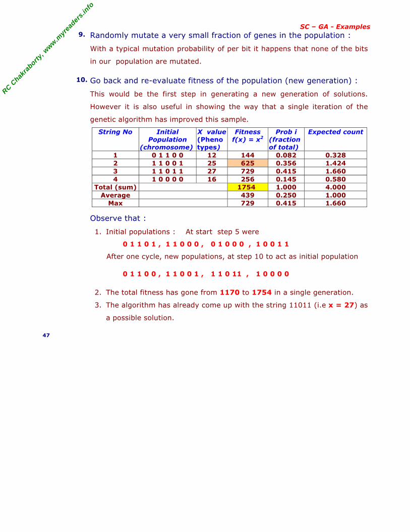
SC – GA - Examples 9. Randomly mutate a very small fraction of genes in the population :
With a typical mutation probability of per bit it happens that none of the bits
in our population are mutated.
10. Go back and re-evaluate fitness of the population (new generation) :
This would be the first step in generating a new generation of solutions.
However it is also useful in showing the way that a single iteration of the
genetic algorithm has improved this sample.
String No Initial Population
(chromosome)
X value(Pheno types)
Fitness f(x) = x2
Prob i (fraction of total)
Expected count
1 0 1 1 0 0 12 144 0.082 0.328 2 1 1 0 0 1 25 625 0.356 1.424 3 1 1 0 1 1 27 729 0.415 1.660 4 1 0 0 0 0 16 256 0.145 0.580
Total (sum) 1754 1.000 4.000 Average 439 0.250 1.000
Max 729 0.415 1.660
Observe that :
1. Initial populations : At start step 5 were
0 1 1 0 1 , 1 1 0 0 0 , 0 1 0 0 0 , 1 0 0 1 1
After one cycle, new populations, at step 10 to act as initial population 0 1 1 0 0 , 1 1 0 0 1 , 1 1 0 11 , 1 0 0 0 0
2. The total fitness has gone from 1170 to 1754 in a single generation.
3. The algorithm has already come up with the string 11011 (i.e x = 27) as
a possible solution.
47
RC C
hakra
borty,
ww
w.m
yrea
ders.
info
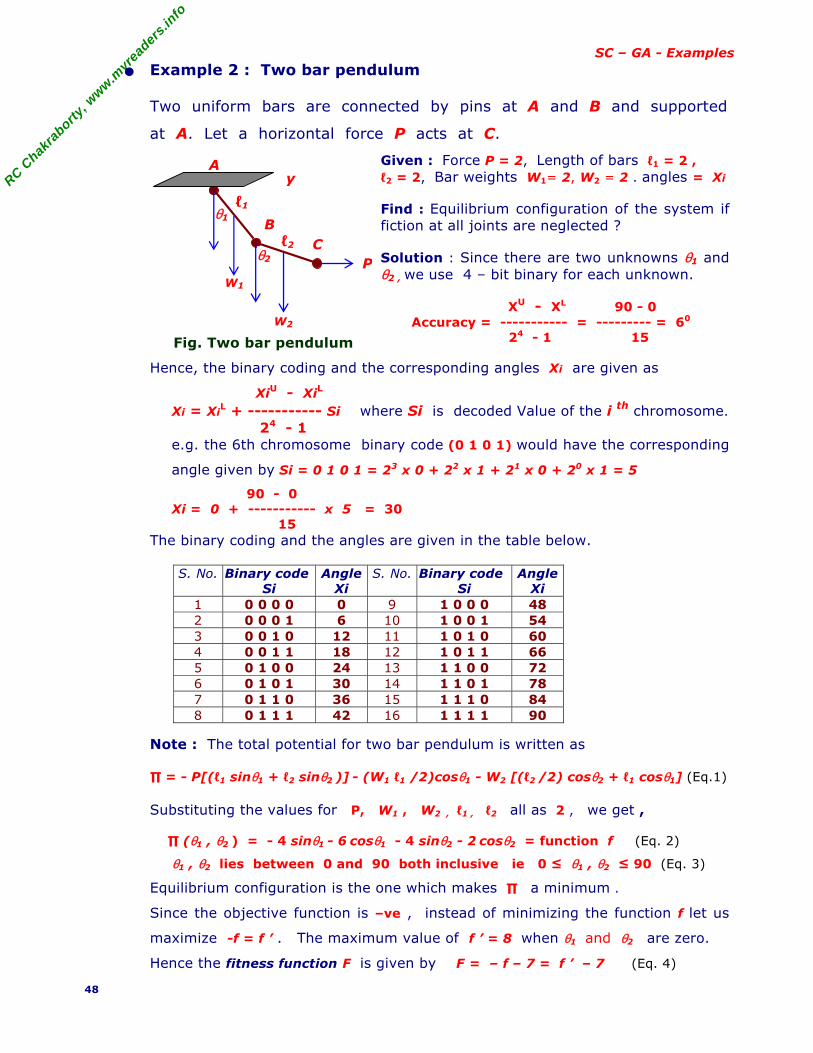
SC – GA - Examples • Example 2 : Two bar pendulum
Two uniform bars are connected by pins at A and B and supported
at A. Let a horizontal force P acts at C.
Fig. Two bar pendulum
Given : Force P = 2, Length of bars ℓ1 = 2 , ℓ2 = 2, Bar weights W1= 2, W2 = 2 . angles = Xi
Find : Equilibrium configuration of the system if fiction at all joints are neglected ? Solution : Since there are two unknowns θ1 and θ2 , we use 4 – bit binary for each unknown.
XU - XL 90 - 0 Accuracy = ----------- = --------- = 60 24 - 1 15
Hence, the binary coding and the corresponding angles Xi are given as
XiU - XiL Xi = Xi
L + ----------- Si where Si is decoded Value of the i th chromosome. 24 - 1 e.g. the 6th chromosome binary code (0 1 0 1) would have the corresponding
angle given by Si = 0 1 0 1 = 23 x 0 + 22 x 1 + 21 x 0 + 20 x 1 = 5
90 - 0 Xi = 0 + ----------- x 5 = 30 15
The binary coding and the angles are given in the table below.
S. No. Binary code Si
AngleXi
S. No. Binary codeSi
AngleXi
1 0 0 0 0 0 9 1 0 0 0 48 2 0 0 0 1 6 10 1 0 0 1 54 3 0 0 1 0 12 11 1 0 1 0 60 4 0 0 1 1 18 12 1 0 1 1 66 5 0 1 0 0 24 13 1 1 0 0 72 6 0 1 0 1 30 14 1 1 0 1 78 7 0 1 1 0 36 15 1 1 1 0 84 8 0 1 1 1 42 16 1 1 1 1 90
Note : The total potential for two bar pendulum is written as
∏ = - P[(ℓ1 sinθ1 + ℓ2 sinθ2 )] - (W1 ℓ1 /2)cosθ1 - W2 [(ℓ2 /2) cosθ2 + ℓ1 cosθ1] (Eq.1)
Substituting the values for P, W1 , W2 , ℓ1 , ℓ2 all as 2 , we get , ∏ (θ1 , θ2 ) = - 4 sinθ1 - 6 cosθ1 - 4 sinθ2 - 2 cosθ2 = function f (Eq. 2)
θ1 , θ2 lies between 0 and 90 both inclusive ie 0 ≤ θ1 , θ2 ≤ 90 (Eq. 3)
Equilibrium configuration is the one which makes ∏ a minimum .
Since the objective function is –ve , instead of minimizing the function f let us
maximize -f = f ’ . The maximum value of f ’ = 8 when θ1 and θ2 are zero.
Hence the fitness function F is given by F = – f – 7 = f ’ – 7 (Eq. 4)
48
W2
W1
y A
θ2
θ1
ℓ2 B
C P
ℓ1
RC C
hakra
borty,
ww
w.m
yrea
ders.
info
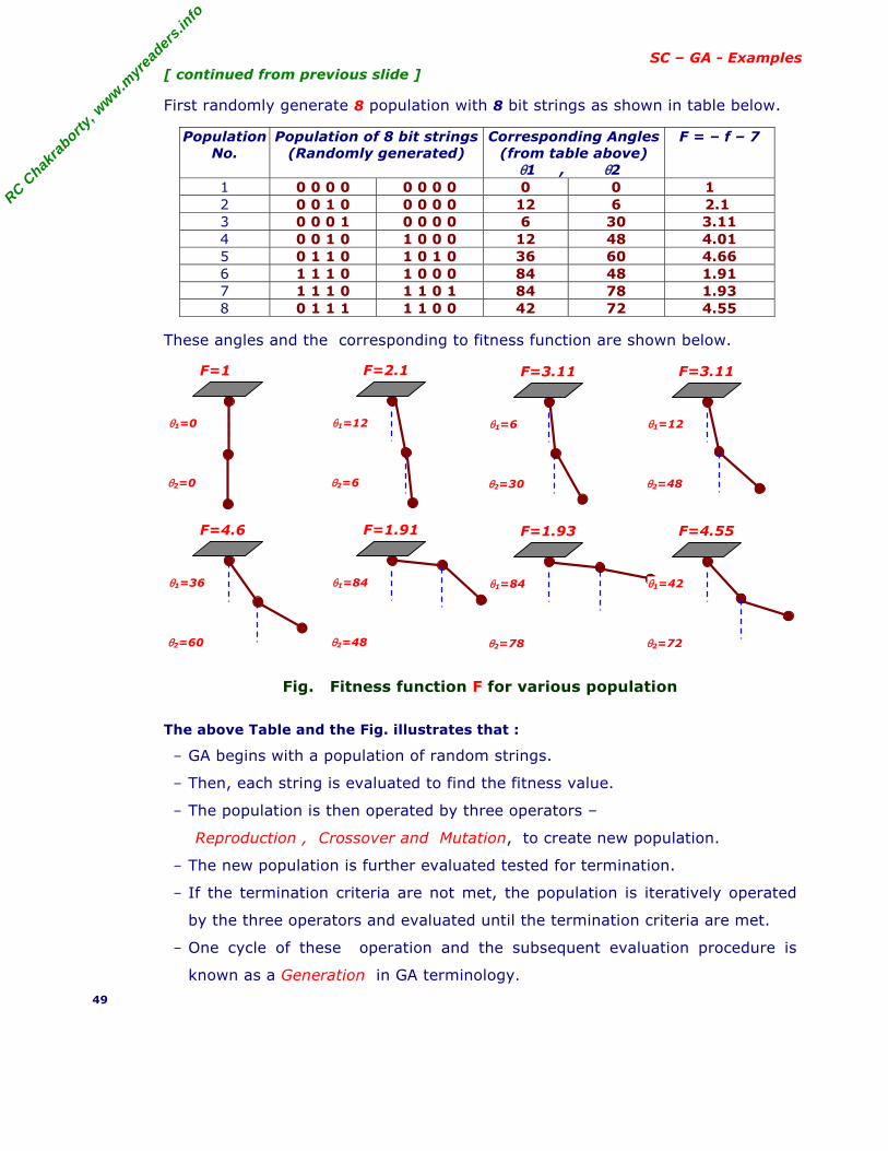
SC – GA - Examples [ continued from previous slide ]
First randomly generate 8 population with 8 bit strings as shown in table below.
PopulationNo.
Population of 8 bit strings(Randomly generated)
Corresponding Angles (from table above)
θ1 , θ2
F = – f – 7
1 0 0 0 0 0 0 0 0 0 0 1 2 0 0 1 0 0 0 0 0 12 6 2.1 3 0 0 0 1 0 0 0 0 6 30 3.11 4 0 0 1 0 1 0 0 0 12 48 4.01 5 0 1 1 0 1 0 1 0 36 60 4.66 6 1 1 1 0 1 0 0 0 84 48 1.91 7 1 1 1 0 1 1 0 1 84 78 1.93 8 0 1 1 1 1 1 0 0 42 72 4.55
These angles and the corresponding to fitness function are shown below.
Fig. Fitness function F for various population
The above Table and the Fig. illustrates that :
− GA begins with a population of random strings.
− Then, each string is evaluated to find the fitness value.
− The population is then operated by three operators –
Reproduction , Crossover and Mutation, to create new population.
− The new population is further evaluated tested for termination.
− If the termination criteria are not met, the population is iteratively operated
by the three operators and evaluated until the termination criteria are met.
− One cycle of these operation and the subsequent evaluation procedure is
known as a Generation in GA terminology.
49
F=1
θ1=0
θ2=0
F=2.1
θ1=12
θ2=6
F=3.11
θ1=6
θ2=30
F=3.11
θ1=12
θ2=48
F=1.91
θ1=84
θ2=48
F=1.93
θ1=84
θ2=78
F=4.55
θ1=42
θ2=72
F=4.6
θ1=36
θ2=60
RC C
hakra
borty,
ww
w.m
yrea
ders.
info
Sc – GA – References 5. References : Textbooks
1. "Neural Network, Fuzzy Logic, and Genetic Algorithms - Synthesis and
Applications", by S. Rajasekaran and G.A. Vijayalaksmi Pai, (2005), Prentice Hall, Chapter 8-9, page 225-293.
2. "Genetic Algorithms in Search, Optimization, and Machine Learning", by David E. Goldberg, (1989), Addison-Wesley, Chapter 1-5, page 1- 214.
3. "An Introduction to Genetic Algorithms", by Melanie Mitchell, (1998), MIT Press, Chapter 1- 5, page 1- 155,
4. "Genetic Algorithms: Concepts And Designs", by K. F. Man, K. S. and Tang, S. Kwong, (201), Springer, Chapter 1- 2, page 1- 42,
5. "Practical genetic algorithms", by Randy L. Haupt, (2004), John Wiley & Sons Inc, Chapter 1- 5, page 1- 127.
6. Related documents from open source, mainly internet. An exhaustive list is being prepared for inclusion at a later date.
50