Embed Size (px)
Citation preview
Genetic Algorithm Niching by (Quasi-)Infinite MemoryAdrian Worring
Computational Biology & Simulation
Group, TU Darmstadt
Darmstadt, Germany
Benjamin E. Mayer
Computational Biology & Simulation
Group, TU Darmstadt
Darmstadt, Germany
Kay Hamacher
Computational Biology & Simulation
Group, TU Darmstadt
Darmstadt, Germany
ABSTRACTGenetic Algorithms (GA) explore the search space of an objective
function via mutation and recombination. Crucial for the search
dynamics is the maintenance of diversity in the population.
Inspired by tabu search we add a mechanism to an elitist GA’s
selection step to ensure diversification by excluding already visited
areas of the search space. To this end, we use Bloom filters as a
probabilistic data structure to store a (quasi-)infinite history.
We discuss how this approach fits into the niching idea for GAs,
finds an analogy in generational correlation via epi-genetics in
biology, and how the approach can be regarded as a co-evolutionary
edge case of previous niching techniques.
Furthermore, we apply this new technique to an NP-hard combi-
natorial optimization problem (ground states of Ising spin glasses).
We find by large-scale hyperparameter scans that our elitist GA
with quasi-infinite memory consistently outperforms its respective
standard GA variant without a Bloom filter.
CCS CONCEPTS• Theory of computation → Tabu search; Bloom filters andhashing; Evolutionary algorithms; •Mathematics of computing→Combinatorial optimization; •Computingmethodologies→ Genetic algorithms.
KEYWORDSGenetic Algorithms, Tabu Search, Combinatorial Optimization,
Hybridization, Population management and niching
ACM Reference Format:Adrian Worring, Benjamin E. Mayer, and Kay Hamacher. 2021. Genetic
Algorithm Niching by (Quasi-)Infinite Memory . In 2021 Genetic and Evolu-tionary Computation Conference (GECCO ’21), July 10–14, 2021, Lille, France.ACM, New York, NY, USA, 9 pages. https://doi.org/10.1145/3449639.3459365
1 INTRODUCTIONSince their inception Genetic Algorithms (GA)[15, 26] are of great
interest to researchers of complex systems, computational sciences,
and mathematics, as well as for practitioners who want to solve
pragmatic optimization problems in a heuristic fashion.
Permission to make digital or hard copies of all or part of this work for personal or
classroom use is granted without fee provided that copies are not made or distributed
for profit or commercial advantage and that copies bear this notice and the full citation
on the first page. Copyrights for components of this work owned by others than ACM
must be honored. Abstracting with credit is permitted. To copy otherwise, or republish,
to post on servers or to redistribute to lists, requires prior specific permission and/or a
fee. Request permissions from [email protected].
GECCO ’21, July 10–14, 2021, Lille, France© 2021 Association for Computing Machinery.
ACM ISBN 978-1-4503-8350-9/21/07. . . $15.00
https://doi.org/10.1145/3449639.3459365
While many aspects of evolutionary dynamics are quite well
understood in principal [20], the quest for optimal evolutionary
schemes and optimal (hyper-)parameters in practical applications is
still ongoing. One way to broaden the applicability and improve the
performance of GA and other evolutionary computing approaches
is niching.
1.1 Niching & Previous WorkThe niching idea [29] takes its motivation from ecology. Typically,
(genetic) diversity on islands and other (geo-)spatially defined re-
gions is higher [17]. A main distinction of niching approaches for
GAs and other evolutionary algorithms – according to Mahfoud
[23] – is spatial vs. temporal niching. Our approach laid out below
(cmp. Sec. 2) couples the whole evolutionary history and thus falls
into temporal niching.
Typically, one employs niching to have an evolutionary algo-
rithm work in separated portions of the search space on (locally)
optimal solutions and multi-objective optimization [11].
Biologically, though, niching also occurs whenever portions of a
genome become inaccessible due to, e.g., epi-genetics (see Sec. 2).
1.2 Tabu Search & Previous WorkThe Tabu Search [13] (TS) method stores individual configurations
in memory and excludes them from future iterations – eventually
excluding any revisit of a potential solution. This increases the
volume of the explored search space and thus diversity. As the
space requirements would increase, one typically implements a
so-called tabu tenure, that is a maximum number of iterations a
visited solution is kept.
1.2.1 Related Work on GAs. The overall idea to include some mem-
orization mechanisms in GAs is not new: Glover et al. [14] dis-
cussed potential hybridization, while Kurahashi and Terano [21]
introduced the idea of a tabu history in determination of parents
during a GA’s recombination phase. They proposed several tabu
lists to achieve different tabu tenures and benchmarked this for
some standard test function in heuristic optimization.
Antony and Jayarajan [1] added a tabu list to an GA with the
explicit goal of diversifying the set of solutions. In data mining, a
similar idea was proposed [22]. Mantawy et al. [24] hybridized GAs
with TS and Simulated Annealing for resource allocation problems.
All this work, however, is characterized by finite tabu tenures,
eventually restricted to a tiny subset of the search space. As soon
as a visited configuration is beyond that, it is “forgotten” and can
be revisited.
296
GECCO ’21, July 10–14, 2021, Lille, France Adrian Worring, Benjamin E. Mayer, and Kay Hamacher
1.2.2 Related Work on Tabu Search. Hamacher [18] combined the
idea of Tabu Search with a variant of Monte-Carlo based optimiza-
tion, namely the Stochastic Tunneling approach [19, 31]. As the
list of visited solutions grows during a run, the tabu list typically
grows as well. The novelty in [18] is based on the usage of a Bloom
filter (see below, Sec. 1.2.3) to work in constant space (and thus also
in constant time for look-up).
1.2.3 Bloom Filter. A Bloom filter [8, 9, 27] is a probabilistic data
structure to determine (approximate) set membership. In its origi-
nal form two operations are available: 1) insertion of an element
and 2) query whether an element is member of the represented set.
Both operations take constant time. The required memory is also
constant and can be chosen beforehand. When testing an element
there is a probability of a false positives. The probability of a false
negative is zero, though. Bloom filters can store an unlimited num-
ber of elements but the false positive rate increases the more are
inserted.
To achieve this a Bloom filter has a bit array of size m and kdifferent hash functions. An empty filter is initialized with all bits
set to zero. To add an element the element e is run through the khash functions resulting in a vector of hashes
ve = [h1(e), . . . ,hk (e)].
For each hash valuehi (e) the bit at indexhi modm in the bit array is
set to 1. When an element is tested the hash functions are evaluated
again and the bits at the positions hi modm are retrieved. If at least
one is 0 the element was never entered to the filter before. If all are
1 the element has possibly been inserted.
It should be emphasized that the hash functions hi do not retain
a “neighborhood” property: although a pair e and e ′might be “close”
in search space the distance betweenhi (e) andhi (e′) is not bounded
at all.
2 TEMPORAL NICHING BY (QUASI-)INFINITEHISTORY
With the rise of epi-genetics, it is a well known biological fact
that not only genetic information is transferred from generation
to generation, but rather also the “availability” is encoded via, e.g.,
methylation patterns [12].
By such mechanisms generations temporally interact while the
underlying (genetic) search space remains. The inclusion of such
additional information and mechanisms allow for faster adaptation
in biological systems. We will minimc this mechanism by excluding
portions of the search space – namely, previously visited configura-
tions – from future accessibility. This implements the Tabu Search
idea and lends itself to niching in biology.
In the notion of Beyer and Schwefel [4] we will use this arising
niching to diversify a GA population in order to cover the search
space of our optimizatin problem more efficiently. We thus leverageniching to increase population diversity for our single goal (to attainthe global optimum) and not as much a method to obtain several
“good” minima.
Using Bloomfilters helps us to achieve a (quasi-)infinite historical
interaction of generations, partition the search space by the search
history, and thus realizes genetic drift in peripatric speciation. We
augment this with a minimal elitist element by allowing for 1% of
individuals to be rescued from the emerging niches into a each new
generation. Note, that due the elitist mechanism a configuration
for a global minima will never enter the Bloom filter.
Our approach can be seen as an extreme form of clearing [28] toeliminate previously (non-elite) solutions.
3 OUR GA VARIANTWITH (QUASI-)INFINITETEMPORAL COUPLING
Algorithm 1 describes our implementation. Solutions are imple-
mented as fixed-length bit strings1. Single-point crossover is used
as recombination operator (CrossOver) and mutations consist of
a single bit flip (Mutate). The crossover locus and the position of
the bit flip are drawn from a uniform random distribution. Multiple
selection methods (Selection-Method) are implemented: Roulette
Wheel Selection, (Exponential) Rank Selection, Truncation Selec-
tion and Tournament Selection. In the subsequent parts we restrict
the choice Selection-Method to tournament selection as the best
performing selection scheme in a preliminary hyperparameter scan.
The nelite
individuals with the best fitness will be carried over to the
next generation without undergoing recombination or mutation
(thus implementing an elitist GA) or filtering by the Bloom filter.
A simple Bloom filter was implemented using the MurmurHash3hash function [2]. Due to this choice, the created hashes do not
retain “neighborhood” as described above and the any false positives
do not create a “forbidden region”, but are (almost) independently
distributed within the whole search space.
After selection, recombination and mutation each individual has
the probability α2 of being tested by the Bloom filter. If the indi-
vidual is found in the filter it will be discarded and a new one will
be selected. Keep in mind that there is a probability of false posi-
tives. So some will be discarded although they were never inserted
into the filter2. Once the next generation has been constructed all
individuals except for the nelite
with the highest fitness have the
probability α1 of being added to the Bloom filter.
For α1 = α2 = 0 we obtain a traditional “non-Bloom” GA.
The implementation is written in C++ and uses xoshiro256** [6]as pseudo-random number generator.
The new method is efficient, whenever creation, mutation, and
recombination is “cheap” in comparison to the evaluation of the
objective function: the Bloom filter criterion might reject several
dozens of configurations per step and only evaluates the objective
function after a (new) individual has passed the Bloom filter crite-
rion. Thus, whenever the computational time is dominated by the
evaluation of the objective function the overhead we introduce is
negligible as Bloom filters work in constant time and space.
4 APPLICATION4.1 A Complex Test InstanceWe apply our new technique to a combinatorial optimization prob-
lemwhich has multiple minima, exponential increase of the number
1This is the natural representation for our test problem in application Section 4. Note,
that this design choice does not imply any restrictions of our Bloom filter idea in other
applications or representations.
2This could potentially also hold for the (unique) global optimum. Pragmatically, one
can either accept this as the algorithm still finds better solution than a “non-Bloom”
variant or increase the Bloom hyperparameters to arbitrarily small false positive rates.
297
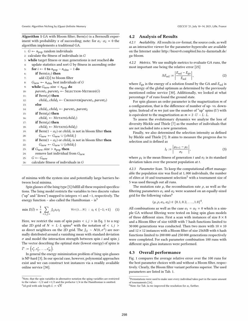
Genetic Algorithm Niching by (Quasi-)Infinite Memory GECCO ’21, July 10–14, 2021, Lille, France
Algorithm 1 GA with Bloom filter; Bern(x) is a Bernoulli exper-iment with probability x of succeeding; note: for α1 ·α2 = 0 the
algorithm implements a traditional GA.
1: G ← npop random individuals
2: calculate the fitness of individuals in G3: while target fitness or max generations is not reached do4: update statistics and sort G by fitness in ascending order
5: for i ← 0 to npop − nelite − 1 do6: if Bern(α1) then7: add G[i] to bloom filter
8: Gnew ← nelite
best individuals of G9: while Gnew.size < npop do10: parent1,parent2 ← Selection-Method(G)11: if Bern(ρ) then12: child1, child2 ← Crossover(parent1,parent2)13: else14: child1, child2 ← parent1,parent215: if Bern(µ) then16: child1 ← Mutate(child1)17: if Bern(µ) then18: child2 ← Mutate(child2)19: if Bern(1 − α2) or child1 is not in bloom filter then20: Gnew ← Gnew ∪ {child1}21: if Bern(1 − α2) or child2 is not in bloom filter then22: Gnew ← Gnew ∪ {child2}23: if Gnew.size > npop then24: remove last individual from Gnew
25: G ← Gnew
26: calculate fitness of individuals in G
of minima with the system size and potentially large barriers be-
tween local minima.
Spin glasses of the Ising type [5] fulfill all these required specifica-
tions. The Ising model restricts the variables to two discrete values
(“up” and “down”) mapped to integers +1 and −1, respectively. The
energy function – also called the Hamiltonian – is3
min E(®s) =1
4
∑<i , j>
Ji jsisj ∀i ∈{1...N } : si ∈ {−1;+1} (1)
Here, we restrict the sum of spin pairs < i, j > in Eq. 1 to a reg-
ular 2D grid of N = L ·L spins4with the notation of < i, j >
as direct neighbors on the 2D grid. The Ji j ∼ N(0,σ2) are nor-
mally distributed around a vanishing mean with standard deviation
σ and model the interaction strength between spin i and spin j.The vector describing the optimal state (lowest energy) of spins is
®s∗ :=(s∗1, s∗2, . . . , s∗N
).
In general the energy minimization problem of Ising spin glasses
is NP-hard [3]. In our special case, however, polynomial approaches
exist and we can construct test instances via a readily available
online service [30].
3Note, that the spin variables in alternative notation the sping variables are restricted
to the values −1/2 and +1/2 and the prefactor 1/4 in the Hamiltonian is omitted.
42d grid with side length L :=
√N
4.2 Analysis of Results4.2.1 Availability. All results in csv-format, the source code, as well
as an interactive viewer for the parameter-hypercube are available
on the Internet under http://biosrv0.compbiol.bio.tu-darmstadt.de/
ga-bloom.
4.2.2 Metrics. We use multiple metrics to evaluate GA runs, the
most important one being the relative error [25]
∆Erel
:=
����Esol − EgaEsol
���� , (2)
where Ega is the energy of a solution found by the GA and Esol
is
the energy of the global optimum as determined by the previously
mentioned online service [30]. Additionally, we looked at what
percentage P of runs found the ground state.
For spin glasses an order parameter is the magnetizationm of
a configuration, that is the difference of number of up- vs. down-
spins. Instead ofm we just use the number of “up” spins (U ) with
is equivalent to the magnetization asm = 2 ·U − L ·L.To assess the evolutionary dynamics we analyze the loss of
diversity Blickle and Thiele [7] as the number of individuals that
are not included into a new generation.
Finally, we also determined the selection intensity as defined
by Blickle and Thiele [7]. It aims to measure the progress due to
selection and is defined as
It :=
���� µt+1 − µtσt
���� , (3)
where µt is the mean fitness of generation t and σt is its standarddeviation taken over the present population at t .
4.2.3 Parameter Scan. To keep the computational effort manage-
able the population size was fixed at 1, 000 individuals, the number
of elites at 10 and tournament selection5with a tournament size of
5 was used through out all runs.
The mutation rate µ, the recombination rate ρ, as well as thefiltering parameters α1 and α2 were scanned on an equally-sized
grid for the following values6
(µ, ρ,α1,α2) ∈ {0.1, 0.2, . . . , 1.0}4.
All combinations as well as the case α1 = α2 = 0 which is a sim-
ple GA without filtering were tested on Ising spin glass models
of three different sizes. First a scan with instances of size 8 × 8
and a Bloom filter of size 64MB with 7 hash functions limited to
30 000 generations was conducted. Then two more with 10 × 10
and 12× 12 instances with a Bloom filter of size 256MB with 6 hash
functions limited to 200 000 and 250 000 generations respectively
were completed. For each parameter combination 100 runs with
different spin glass instances were performed.
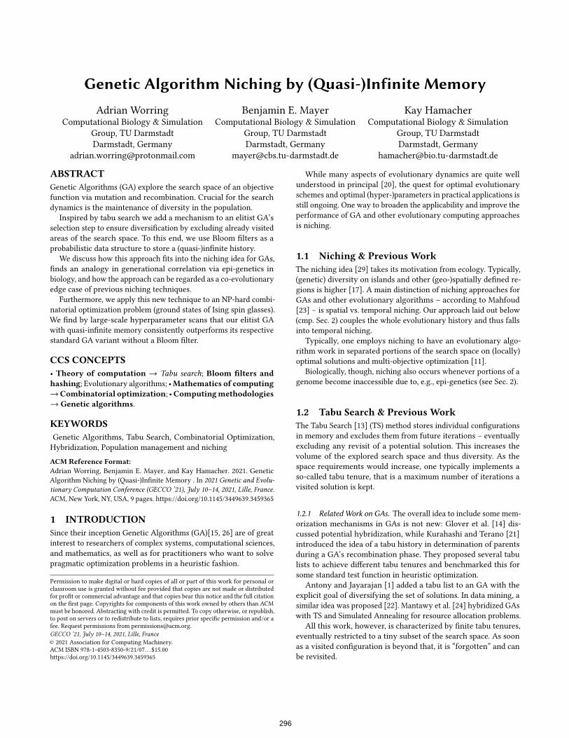
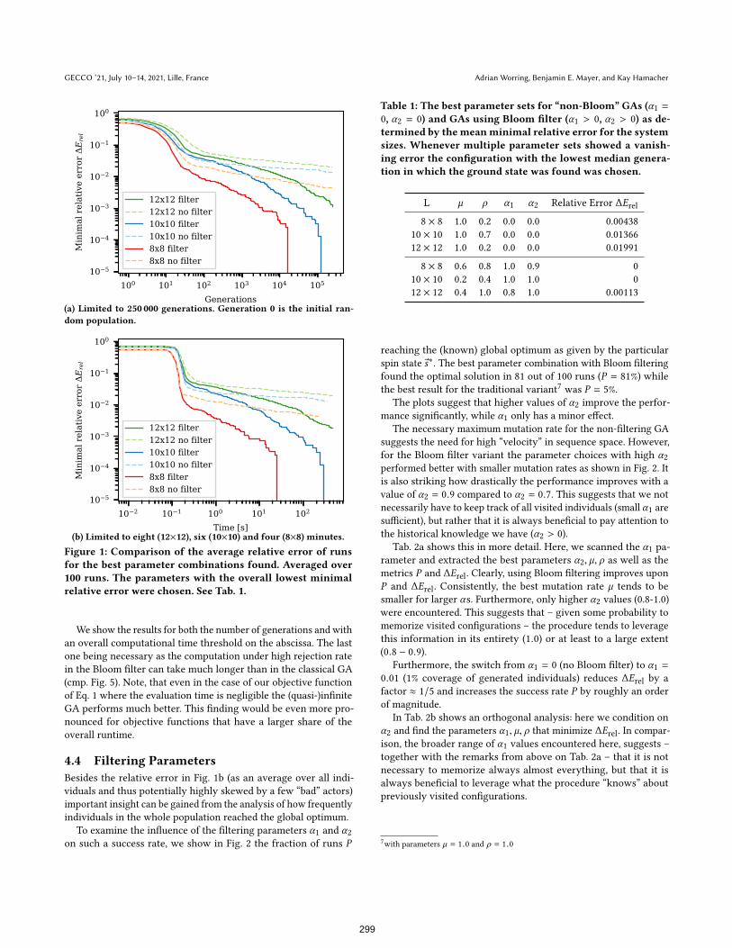
4.3 Overall performanceFig. 1 compares the average relative error over the 100 runs for
the best parameter choices with and without a Bloom filter, respec-
tively. Clearly, the Bloom filter variant performs superior. The used
parameters are listed in Tab. 1.
5Permutations were used to make sure every individual takes part in the same amount
of tournaments [16].
6Note: for Tab. 2a we improved the resolution for α1 further.
298
GECCO ’21, July 10–14, 2021, Lille, France Adrian Worring, Benjamin E. Mayer, and Kay Hamacher
100 101 102 103 104 105
Generations
10−5
10−4
10−3
10−2
10−1
100
Min
imal
rel
ativ
e er
ror
ΔErel
12x12 filter12x12 no filter10x10 filter10x10 no filter8x8 filter8x8 no filter
(a) Limited to 250 000 generations. Generation 0 is the initial ran-dom population.
10−2 10−1 100 101 102
Time [s]
10−5
10−4
10−3
10−2
10−1
100
Min
imal
rel
ativ
e er
ror
ΔErel
12x12 filter12x12 no filter10x10 filter10x10 no filter8x8 filter8x8 no filter
(b) Limited to eight (12×12), six (10×10) and four (8×8) minutes.
Figure 1: Comparison of the average relative error of runsfor the best parameter combinations found. Averaged over100 runs. The parameters with the overall lowest minimalrelative error were chosen. See Tab. 1.
We show the results for both the number of generations and with
an overall computational time threshold on the abscissa. The last
one being necessary as the computation under high rejection rate
in the Bloom filter can take much longer than in the classical GA
(cmp. Fig. 5). Note, that even in the case of our objective function
of Eq. 1 where the evaluation time is negligible the (quasi-)infinite
GA performs much better. This finding would be even more pro-
nounced for objective functions that have a larger share of the
overall runtime.
4.4 Filtering ParametersBesides the relative error in Fig. 1b (as an average over all indi-
viduals and thus potentially highly skewed by a few “bad” actors)
important insight can be gained from the analysis of how frequently
individuals in the whole population reached the global optimum.
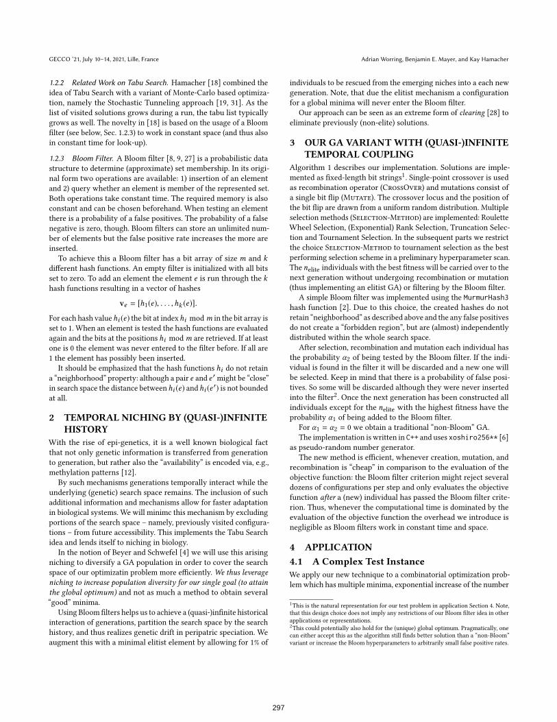
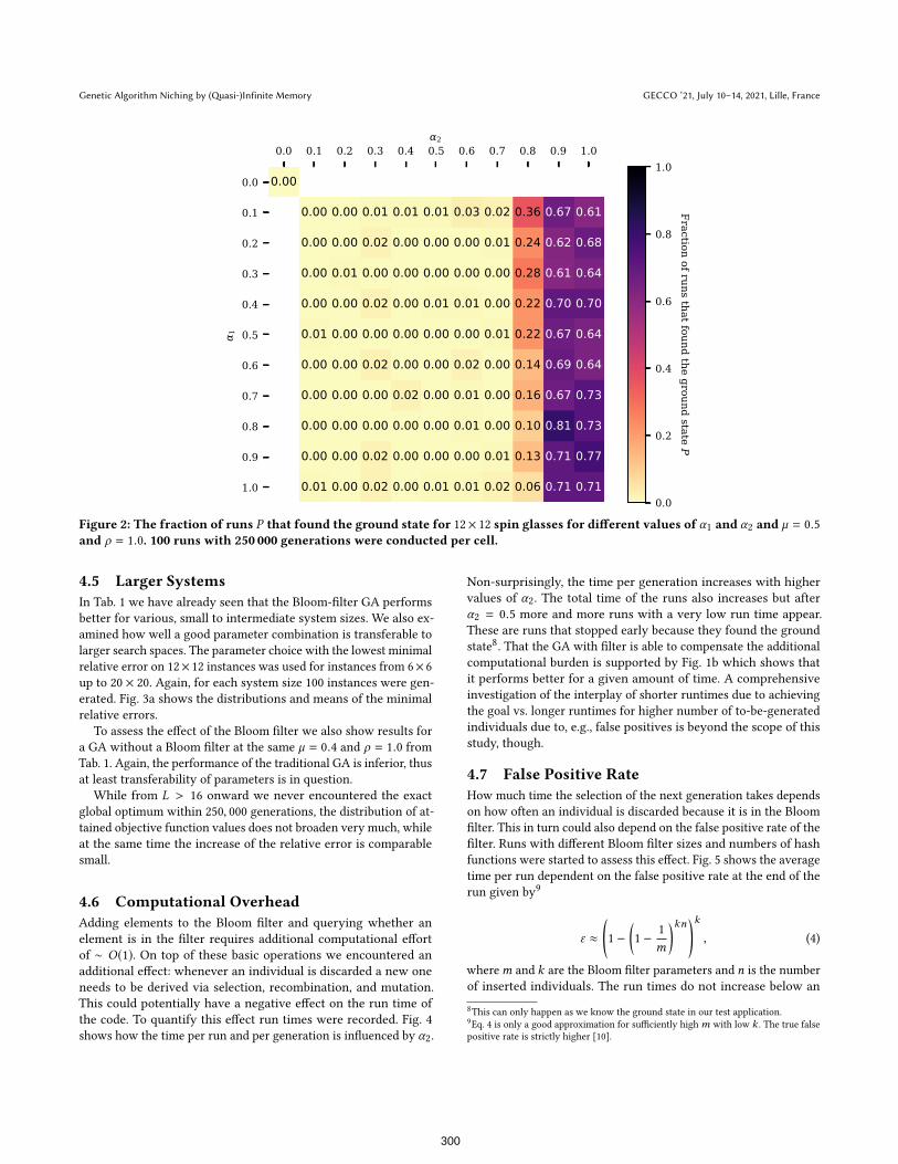
To examine the influence of the filtering parameters α1 and α2on such a success rate, we show in Fig. 2 the fraction of runs P
Table 1: The best parameter sets for “non-Bloom” GAs (α1 =0, α2 = 0) and GAs using Bloom filter (α1 > 0, α2 > 0) as de-termined by themeanminimal relative error for the systemsizes. Whenever multiple parameter sets showed a vanish-ing error the configuration with the lowest median genera-tion in which the ground state was found was chosen.
L µ ρ α1 α2 Relative Error ∆Erel
8 × 8 1.0 0.2 0.0 0.0 0.00438
10 × 10 1.0 0.7 0.0 0.0 0.01366
12 × 12 1.0 0.2 0.0 0.0 0.01991
8 × 8 0.6 0.8 1.0 0.9 0
10 × 10 0.2 0.4 1.0 1.0 0
12 × 12 0.4 1.0 0.8 1.0 0.00113
reaching the (known) global optimum as given by the particular
spin state ®s∗. The best parameter combination with Bloom filtering
found the optimal solution in 81 out of 100 runs (P = 81%) while
the best result for the traditional variant7was P = 5%.
The plots suggest that higher values of α2 improve the perfor-
mance significantly, while α1 only has a minor effect.
The necessary maximum mutation rate for the non-filtering GA
suggests the need for high “velocity” in sequence space. However,
for the Bloom filter variant the parameter choices with high α2performed better with smaller mutation rates as shown in Fig. 2. It
is also striking how drastically the performance improves with a
value of α2 = 0.9 compared to α2 = 0.7. This suggests that we not
necessarily have to keep track of all visited individuals (small α1 aresufficient), but rather that it is always beneficial to pay attention to
the historical knowledge we have (α2 > 0).
Tab. 2a shows this in more detail. Here, we scanned the α1 pa-rameter and extracted the best parameters α2, µ, ρ as well as the
metrics P and ∆Erel. Clearly, using Bloom filtering improves upon
P and ∆Erel. Consistently, the best mutation rate µ tends to be
smaller for larger αs. Furthermore, only higher α2 values (0.8-1.0)were encountered. This suggests that – given some probability to
memorize visited configurations – the procedure tends to leverage
this information in its entirety (1.0) or at least to a large extent
(0.8 − 0.9).
Furthermore, the switch from α1 = 0 (no Bloom filter) to α1 =0.01 (1% coverage of generated individuals) reduces ∆E
relby a
factor ≈ 1/5 and increases the success rate P by roughly an order
of magnitude.
In Tab. 2b shows an orthogonal analysis: here we condition on
α2 and find the parameters α1, µ, ρ that minimize ∆Erel. In compar-
ison, the broader range of α1 values encountered here, suggests –
together with the remarks from above on Tab. 2a – that it is not
necessary to memorize always almost everything, but that it is
always beneficial to leverage what the procedure “knows” about
previously visited configurations.
7with parameters µ = 1.0 and ρ = 1.0
299
Genetic Algorithm Niching by (Quasi-)Infinite Memory GECCO ’21, July 10–14, 2021, Lille, France
0.0 0.1 0.2 0.3 0.4 0.5 0.6 0.7 0.8 0.9 1.0α2
0.0
0.1
0.2
0.3
0.4
0.5
0.6
0.7
0.8
0.9
1.0
α 1
0.00
0.00 0.00 0.01 0.01 0.01 0.03 0.02 0.36 0.67 0.61
0.00 0.00 0.02 0.00 0.00 0.00 0.01 0.24 0.62 0.68
0.00 0.01 0.00 0.00 0.00 0.00 0.00 0.28 0.61 0.64
0.00 0.00 0.02 0.00 0.01 0.01 0.00 0.22 0.70 0.70
0.01 0.00 0.00 0.00 0.00 0.00 0.01 0.22 0.67 0.64
0.00 0.00 0.02 0.00 0.00 0.02 0.00 0.14 0.69 0.64
0.00 0.00 0.00 0.02 0.00 0.01 0.00 0.16 0.67 0.73
0.00 0.00 0.00 0.00 0.00 0.01 0.00 0.10 0.81 0.73
0.00 0.00 0.02 0.00 0.00 0.00 0.01 0.13 0.71 0.77
0.01 0.00 0.02 0.00 0.01 0.01 0.02 0.06 0.71 0.710.0
0.2
0.4
0.6
0.8
1.0
Fraction of runs that found the ground state P
Figure 2: The fraction of runs P that found the ground state for 12× 12 spin glasses for different values of α1 and α2 and µ = 0.5
and ρ = 1.0. 100 runs with 250 000 generations were conducted per cell.
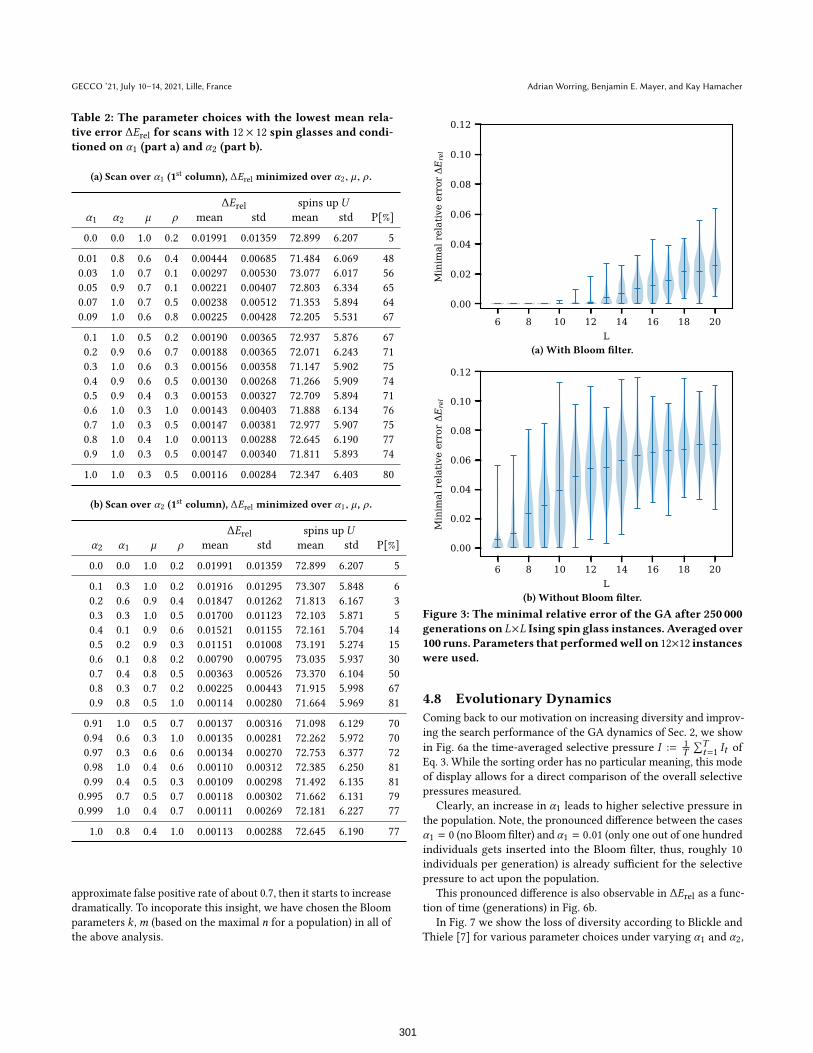
4.5 Larger SystemsIn Tab. 1 we have already seen that the Bloom-filter GA performs
better for various, small to intermediate system sizes. We also ex-
amined how well a good parameter combination is transferable to
larger search spaces. The parameter choice with the lowest minimal
relative error on 12× 12 instances was used for instances from 6× 6
up to 20 × 20. Again, for each system size 100 instances were gen-
erated. Fig. 3a shows the distributions and means of the minimal
relative errors.
To assess the effect of the Bloom filter we also show results for
a GA without a Bloom filter at the same µ = 0.4 and ρ = 1.0 from
Tab. 1. Again, the performance of the traditional GA is inferior, thus
at least transferability of parameters is in question.
While from L > 16 onward we never encountered the exact
global optimum within 250, 000 generations, the distribution of at-
tained objective function values does not broaden very much, while
at the same time the increase of the relative error is comparable
small.
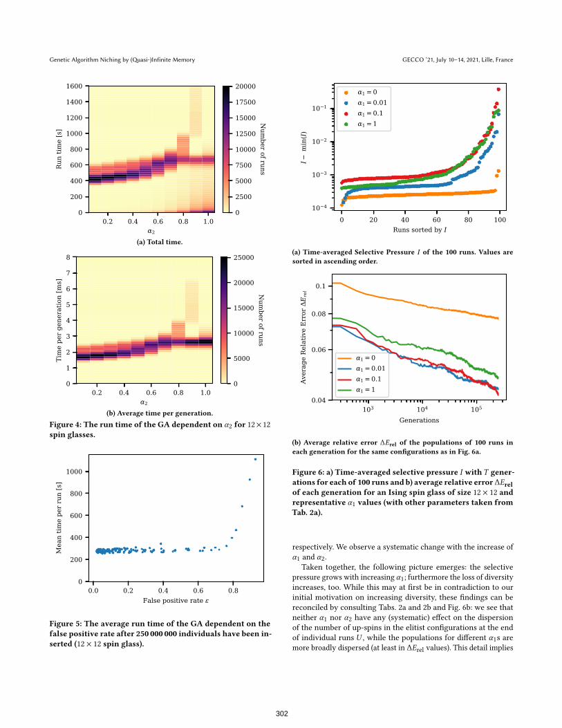
4.6 Computational OverheadAdding elements to the Bloom filter and querying whether an
element is in the filter requires additional computational effort
of ∼ O(1). On top of these basic operations we encountered an
additional effect: whenever an individual is discarded a new one
needs to be derived via selection, recombination, and mutation.
This could potentially have a negative effect on the run time of
the code. To quantify this effect run times were recorded. Fig. 4
shows how the time per run and per generation is influenced by α2.
Non-surprisingly, the time per generation increases with higher
values of α2. The total time of the runs also increases but after
α2 = 0.5 more and more runs with a very low run time appear.
These are runs that stopped early because they found the ground
state8. That the GA with filter is able to compensate the additional
computational burden is supported by Fig. 1b which shows that
it performs better for a given amount of time. A comprehensive
investigation of the interplay of shorter runtimes due to achieving
the goal vs. longer runtimes for higher number of to-be-generated
individuals due to, e.g., false positives is beyond the scope of this
study, though.
4.7 False Positive RateHow much time the selection of the next generation takes depends
on how often an individual is discarded because it is in the Bloom
filter. This in turn could also depend on the false positive rate of the
filter. Runs with different Bloom filter sizes and numbers of hash
functions were started to assess this effect. Fig. 5 shows the average
time per run dependent on the false positive rate at the end of the
run given by9
ε ≈
(1 −
(1 −
1
m
)kn )k, (4)
wherem and k are the Bloom filter parameters and n is the number
of inserted individuals. The run times do not increase below an
8This can only happen as we know the ground state in our test application.
9Eq. 4 is only a good approximation for sufficiently highm with low k . The true falsepositive rate is strictly higher [10].
300
GECCO ’21, July 10–14, 2021, Lille, France Adrian Worring, Benjamin E. Mayer, and Kay Hamacher
Table 2: The parameter choices with the lowest mean rela-tive error ∆E
relfor scans with 12 × 12 spin glasses and condi-
tioned on α1 (part a) and α2 (part b).
(a) Scan over α1 (1st column), ∆Erel
minimized over α2, µ , ρ .
∆Erel
spins upUα1 α2 µ ρ mean std mean std P[%]
0.0 0.0 1.0 0.2 0.01991 0.01359 72.899 6.207 5
0.01 0.8 0.6 0.4 0.00444 0.00685 71.484 6.069 48
0.03 1.0 0.7 0.1 0.00297 0.00530 73.077 6.017 56
0.05 0.9 0.7 0.1 0.00221 0.00407 72.803 6.334 65
0.07 1.0 0.7 0.5 0.00238 0.00512 71.353 5.894 64
0.09 1.0 0.6 0.8 0.00225 0.00428 72.205 5.531 67
0.1 1.0 0.5 0.2 0.00190 0.00365 72.937 5.876 67
0.2 0.9 0.6 0.7 0.00188 0.00365 72.071 6.243 71
0.3 1.0 0.6 0.3 0.00156 0.00358 71.147 5.902 75
0.4 0.9 0.6 0.5 0.00130 0.00268 71.266 5.909 74
0.5 0.9 0.4 0.3 0.00153 0.00327 72.709 5.894 71
0.6 1.0 0.3 1.0 0.00143 0.00403 71.888 6.134 76
0.7 1.0 0.3 0.5 0.00147 0.00381 72.977 5.907 75
0.8 1.0 0.4 1.0 0.00113 0.00288 72.645 6.190 77
0.9 1.0 0.3 0.5 0.00147 0.00340 71.811 5.893 74
1.0 1.0 0.3 0.5 0.00116 0.00284 72.347 6.403 80
(b) Scan over α2 (1st column), ∆Erel
minimized over α1, µ , ρ .
∆Erel
spins upUα2 α1 µ ρ mean std mean std P[%]
0.0 0.0 1.0 0.2 0.01991 0.01359 72.899 6.207 5
0.1 0.3 1.0 0.2 0.01916 0.01295 73.307 5.848 6
0.2 0.6 0.9 0.4 0.01847 0.01262 71.813 6.167 3
0.3 0.3 1.0 0.5 0.01700 0.01123 72.103 5.871 5
0.4 0.1 0.9 0.6 0.01521 0.01155 72.161 5.704 14
0.5 0.2 0.9 0.3 0.01151 0.01008 73.191 5.274 15
0.6 0.1 0.8 0.2 0.00790 0.00795 73.035 5.937 30
0.7 0.4 0.8 0.5 0.00363 0.00526 73.370 6.104 50
0.8 0.3 0.7 0.2 0.00225 0.00443 71.915 5.998 67
0.9 0.8 0.5 1.0 0.00114 0.00280 71.664 5.969 81
0.91 1.0 0.5 0.7 0.00137 0.00316 71.098 6.129 70
0.94 0.6 0.3 1.0 0.00135 0.00281 72.262 5.972 70
0.97 0.3 0.6 0.6 0.00134 0.00270 72.753 6.377 72
0.98 1.0 0.4 0.6 0.00110 0.00312 72.385 6.250 81
0.99 0.4 0.5 0.3 0.00109 0.00298 71.492 6.135 81
0.995 0.7 0.5 0.7 0.00118 0.00302 71.662 6.131 79
0.999 1.0 0.4 0.7 0.00111 0.00269 72.181 6.227 77
1.0 0.8 0.4 1.0 0.00113 0.00288 72.645 6.190 77
approximate false positive rate of about 0.7, then it starts to increase
dramatically. To incoporate this insight, we have chosen the Bloom
parameters k ,m (based on the maximal n for a population) in all of
the above analysis.
6 8 10 12 14 16 18 20L
0.00
0.02
0.04
0.06
0.08
0.10
0.12
Min
imal
rel
ativ
e er
ror
ΔErel
(a) With Bloom filter.
6 8 10 12 14 16 18 20L
0.00
0.02
0.04
0.06
0.08
0.10
0.12
Min
imal
rel
ativ
e er
ror
ΔErel
(b) Without Bloom filter.
Figure 3: The minimal relative error of the GA after 250 000generations on L×L Ising spin glass instances. Averaged over100 runs. Parameters that performedwell on 12×12 instanceswere used.
4.8 Evolutionary DynamicsComing back to our motivation on increasing diversity and improv-
ing the search performance of the GA dynamics of Sec. 2, we show
in Fig. 6a the time-averaged selective pressure I := 1
T∑Tt=1 It of
Eq. 3. While the sorting order has no particular meaning, this mode
of display allows for a direct comparison of the overall selective
pressures measured.
Clearly, an increase in α1 leads to higher selective pressure in
the population. Note, the pronounced difference between the cases
α1 = 0 (no Bloom filter) and α1 = 0.01 (only one out of one hundred
individuals gets inserted into the Bloom filter, thus, roughly 10
individuals per generation) is already sufficient for the selective
pressure to act upon the population.
This pronounced difference is also observable in ∆Erel
as a func-
tion of time (generations) in Fig. 6b.
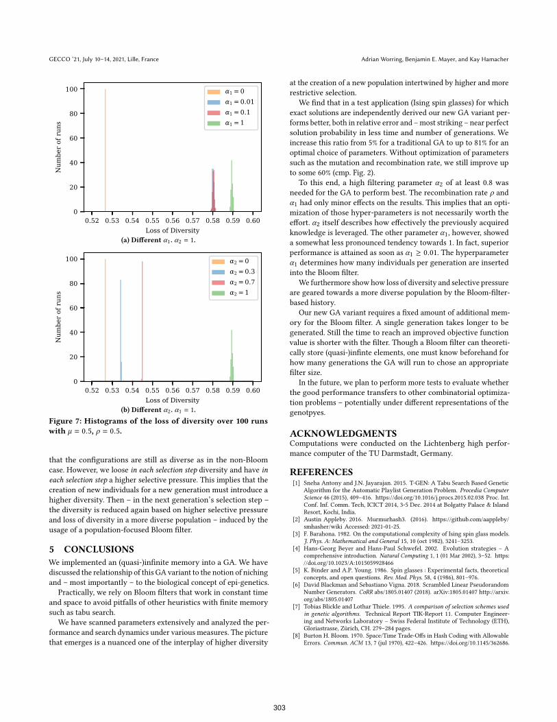
In Fig. 7 we show the loss of diversity according to Blickle and
Thiele [7] for various parameter choices under varying α1 and α2,
301
Genetic Algorithm Niching by (Quasi-)Infinite Memory GECCO ’21, July 10–14, 2021, Lille, France
0.2 0.4 0.6 0.8 1.0α2
0
200
400
600
800
1000
1200
1400
1600
Run
tim
e [s
]
0
2500
5000
7500
10000
12500
15000
17500
20000
Num
ber of runs
(a) Total time.
0.2 0.4 0.6 0.8 1.0α2
0
1
2
3
4
5
6
7
8
Tim
e pe
r ge
nera
tion
[ms]
0
5000
10000
15000
20000
25000
Num
ber of runs
(b) Average time per generation.
Figure 4: The run time of the GA dependent on α2 for 12× 12spin glasses.
0.0 0.2 0.4 0.6 0.8False positive rate ε
0
200
400
600
800
1000
Mea
n tim
e pe
r ru
n [s
]
Figure 5: The average run time of the GA dependent on thefalse positive rate after 250 000 000 individuals have been in-serted (12 × 12 spin glass).
0 20 40 60 80 100Runs sorted by I
10−4
10−3
10−2
10−1
I− m
in(I
)
α1 = 0α1 = 0.01α1 = 0.1α1 = 1
(a) Time-averaged Selective Pressure I of the 100 runs. Values aresorted in ascending order.
103 104 105
Generations
0.04
0.06
0.08
0.1
Aver
age
Rel
ativ
e E
rror
ΔErel
α1 = 0α1 = 0.01α1 = 0.1α1 = 1
(b) Average relative error ∆Erel of the populations of 100 runs ineach generation for the same configurations as in Fig. 6a.
Figure 6: a) Time-averaged selective pressure I withT gener-ations for each of 100 runs and b) average relative error ∆Erelof each generation for an Ising spin glass of size 12 × 12 andrepresentative α1 values (with other parameters taken fromTab. 2a).
respectively. We observe a systematic change with the increase of
α1 and α2.Taken together, the following picture emerges: the selective
pressure grows with increasing α1; furthermore the loss of diversity
increases, too. While this may at first be in contradiction to our
initial motivation on increasing diversity, these findings can be
reconciled by consulting Tabs. 2a and 2b and Fig. 6b: we see that
neither α1 nor α2 have any (systematic) effect on the dispersion
of the number of up-spins in the elitist configurations at the end
of individual runs U , while the populations for different α1s aremore broadly dispersed (at least in ∆E
relvalues). This detail implies
302
GECCO ’21, July 10–14, 2021, Lille, France Adrian Worring, Benjamin E. Mayer, and Kay Hamacher
0.52 0.53 0.54 0.55 0.56 0.57 0.58 0.59 0.60Loss of Diversity
0
20
40
60
80
100
Num
ber
of r
uns
α1 = 0α1 = 0.01α1 = 0.1α1 = 1
(a) Different α1. α2 = 1.
0.52 0.53 0.54 0.55 0.56 0.57 0.58 0.59 0.60Loss of Diversity
0
20
40
60
80
100
Num
ber
of r
uns
α2 = 0α2 = 0.3α2 = 0.7α2 = 1
(b) Different α2. α1 = 1.
Figure 7: Histograms of the loss of diversity over 100 runswith µ = 0.5, ρ = 0.5.
that the configurations are still as diverse as in the non-Bloom
case. However, we loose in each selection step diversity and have ineach selection step a higher selective pressure. This implies that the
creation of new individuals for a new generation must introduce a
higher diversity. Then – in the next generation’s selection step –
the diversity is reduced again based on higher selective pressure
and loss of diversity in a more diverse population – induced by the
usage of a population-focused Bloom filter.
5 CONCLUSIONSWe implemented an (quasi-)infinite memory into a GA. We have
discussed the relationship of this GA variant to the notion of niching
and – most importantly – to the biological concept of epi-genetics.
Practically, we rely on Bloom filters that work in constant time
and space to avoid pitfalls of other heuristics with finite memory
such as tabu search.
We have scanned parameters extensively and analyzed the per-
formance and search dynamics under various measures. The picture
that emerges is a nuanced one of the interplay of higher diversity
at the creation of a new population intertwined by higher and more
restrictive selection.
We find that in a test application (Ising spin glasses) for which
exact solutions are independently derived our new GA variant per-
forms better, both in relative error and –most striking – near perfect
solution probability in less time and number of generations. We
increase this ratio from 5% for a traditional GA to up to 81% for an
optimal choice of parameters. Without optimization of parameters
such as the mutation and recombination rate, we still improve up
to some 60% (cmp. Fig. 2).
To this end, a high filtering parameter α2 of at least 0.8 was
needed for the GA to perform best. The recombination rate ρ and
α1 had only minor effects on the results. This implies that an opti-
mization of those hyper-parameters is not necessarily worth the
effort. α2 itself describes how effectively the previously acquired
knowledge is leveraged. The other parameter α1, however, showeda somewhat less pronounced tendency towards 1. In fact, superior
performance is attained as soon as α1 ≥ 0.01. The hyperparameter
α1 determines how many individuals per generation are inserted
into the Bloom filter.
We furthermore showhow loss of diversity and selective pressure
are geared towards a more diverse population by the Bloom-filter-
based history.
Our new GA variant requires a fixed amount of additional mem-
ory for the Bloom filter. A single generation takes longer to be
generated. Still the time to reach an improved objective function
value is shorter with the filter. Though a Bloom filter can theoreti-
cally store (quasi-)infinte elements, one must know beforehand for
how many generations the GA will run to chose an appropriate
filter size.
In the future, we plan to perform more tests to evaluate whether
the good performance transfers to other combinatorial optimiza-
tion problems – potentially under different representations of the
genotpyes.
ACKNOWLEDGMENTSComputations were conducted on the Lichtenberg high perfor-
mance computer of the TU Darmstadt, Germany.
REFERENCES[1] Sneha Antony and J.N. Jayarajan. 2015. T-GEN: A Tabu Search Based Genetic
Algorithm for the Automatic Playlist Generation Problem. Procedia ComputerScience 46 (2015), 409–416. https://doi.org/10.1016/j.procs.2015.02.038 Proc. Int.
Conf. Inf. Comm. Tech, ICICT 2014, 3-5 Dec. 2014 at Bolgatty Palace & Island
Resort, Kochi, India.
[2] Austin Appleby. 2016. Murmurhash3. (2016). https://github.com/aappleby/
smhasher/wiki Accessed: 2021-01-25.
[3] F. Barahona. 1982. On the computational complexity of Ising spin glass models.
J. Phys. A: Mathematical and General 15, 10 (oct 1982), 3241–3253.[4] Hans-Georg Beyer and Hans-Paul Schwefel. 2002. Evolution strategies – A
comprehensive introduction. Natural Computing 1, 1 (01 Mar 2002), 3–52. https:
//doi.org/10.1023/A:1015059928466
[5] K. Binder and A.P. Young. 1986. Spin glasses : Experimental facts, theoretical
concepts, and open questions. Rev. Mod. Phys. 58, 4 (1986), 801–976.[6] David Blackman and Sebastiano Vigna. 2018. Scrambled Linear Pseudorandom
Number Generators. CoRR abs/1805.01407 (2018). arXiv:1805.01407 http://arxiv.
org/abs/1805.01407
[7] Tobias Blickle and Lothar Thiele. 1995. A comparison of selection schemes usedin genetic algorithms. Technical Report TIK-Report 11. Computer Engineer-
ing and Networks Laboratory – Swiss Federal Institute of Technology (ETH),
Gloriastrasse, Zürich, CH. 279–284 pages.
[8] Burton H. Bloom. 1970. Space/Time Trade-Offs in Hash Coding with Allowable
Errors. Commun. ACM 13, 7 (jul 1970), 422–426. https://doi.org/10.1145/362686.
303
Genetic Algorithm Niching by (Quasi-)Infinite Memory GECCO ’21, July 10–14, 2021, Lille, France
362692
[9] James Blustein and Amal El-Maazawi. 2002. Bloom filters. A tutorial, analysis, andsurvey. Technical Report. Dalhousie University, Halifax, Nova Scotia. 1–31 pages.https://cdn.dal.ca/content/dam/dalhousie/pdf/faculty/computerscience/technical-
reports/CS-2002-10.pdf; accessed 04/06/2021.
[10] Prosenjit Bose, Hua Guo, Evangelos Kranakis, Anil Maheshwari, Pat Morin, Jason
Morrison, Michiel Smid, and Yihui Tang. 2008. On the false-positive rate of Bloom
filters. Inform. Process. Lett. 108, 4 (2008), 210 – 213. https://doi.org/10.1016/j.ipl.
2008.05.018
[11] Kalyanmoy Deb. 2001. Multi-objective optimization using evolutionary algorithms.John Wiley & Sons, Chichester New York.
[12] Cathérine Dupont, D. Randall Armant, and Carol A. Brenner. 2009. Epige-
netics: definition, mechanisms and clinical perspective. Seminars in reproduc-tive medicine 27, 5 (Sep 2009), 351–357. https://doi.org/10.1055/s-0029-1237423
19711245[pmid].
[13] Fred Glover. 1989. Tabu Search—Part I. ORSA Journal on Computing 1, 3 (1989),
190–206. https://doi.org/10.1287/ijoc.1.3.190
[14] Fred Glover, James P. Kelly, and Manuel Laguna. 1995. Genetic algorithms and
tabu search: Hybrids for optimization. Comp. & Op. Res. 22, 1 (1995), 111–134.https://doi.org/10.1016/0305-0548(93)E0023-M
[15] David E. Goldberg. 1989. Genetic Algorithms in Search, Optimization, and MachineLearning. Addison-Wesley, Reading, Massachusetts.
[16] David E. Goldberg, Bradley Korb, and Kalyanmoy Deb. 1989. Messy Genetic
Algorithms: Motivation, Analysis, and First Results. Complex Syst. 3, 5 (1989).[17] Natalie Graham, Daniel S. Gruner, Jun Y. Lim, and Rosemary G. Gillespie. 2017.
Island ecology and evolution: challenges in the anthropocene. EnvironmentalConservation 44, 4 (2017), 323–335. https://doi.org/10.1017/s0376892917000315
[18] K. Hamacher. 2019. Hybridization of Stochastic Tunneling with (Quasi)-Infinite
Time-Horizon Tabu Search. InHybridMetaheuristics, M. J. Blesa Aguilera, C. Blum,
H. Gambini Santos, P. Pinacho-Davidson, and J. Godoy del Campo (Eds.). Springer
International Publishing, Cham, 124–135.
[19] K. Hamacher and W. Wenzel. 1999. The Scaling Behaviour of Stochastic Min-
imization Algorithms in a Perfect Funnel Landscape. Phys. Rev. E 59, 1 (1999),
938–941.
[20] John H. Holland. 1992. Adapation in Natural and Artifical Systems. MIT Press,
Cambridge, Massachusetts.
[21] Setsuya Kurahashi and Takao Terano. 2000. A Genetic Algorithm with Tabu
Search for Multimodal and Multiobjective Function Optimization. In Proceed-ings of the 2nd Annual Conference on Genetic and Evolutionary Computation(GECCO’00). Morgan Kaufmann Publishers Inc., San Francisco, CA, USA, 291–
298.
[22] F. M. Lopes and A. T. R. Pozo. 2001. Genetic algorithm restricted by tabu lists in
data mining. In SCCC 2001. 21st International Conference of the Chilean ComputerScience Society. 178–185. https://doi.org/10.1109/SCCC.2001.972646
[23] Samir W. Mahfoud and Samir W. Mahfoud. 1995. A Comparison of Parallel
and Sequential Niching Methods. In In Proceedings of the Sixth InternationalConference on Genetic Algorithms. Morgan Kaufmann, 136–143.
[24] A. H. Mantawy, Y. L. Abdel-Magid, and S. Z. Selim. 1999. Integrating genetic algo-
rithms, tabu search, and simulated annealing for the unit commitment problem.
IEEE Trans. Power Sys. 14, 3 (1999), 829–836. https://doi.org/10.1109/59.780892[25] B. E. Mayer and K. Hamacher. 2014. Stochastic Tunneling Transformation during
Selection in Genetic Algorithm. In Proceedings of the 2014 Annual Conference onGenetic and Evolutionary Computation (GECCO ’14). Association for Comput-
ing Machinery, New York, NY, USA, 801–806. https://doi.org/10.1145/2576768.
2598243
[26] Melanie Mitchell. 1996. An introduction to genetic algorithms. MIT Press, Cam-
bridge, Massachusetts.
[27] Michael Mitzenmacher. 2002. Compressed bloom filters. IEEE/ACM Trans. Netw.10, 5 (2002), 604–612.
[28] A. Petrowski. 1996. A clearing procedure as a niching method for genetic al-
gorithms. In Proc. IEEE Int. Conf. Evol. Comp. IEEE, 798–803. https://doi.org/10.1109/ICEC.1996.542703
[29] Ofer M. Shir. 2012. Niching in Evolutionary Algorithms. In Handbook of NaturalComputing, Grzegorz Rozenberg, Thomas Bäck, and Joost N. Kok (Eds.). Springer
Berlin Heidelberg, Berlin, Heidelberg, 1035–1069. https://doi.org/10.1007/978-3-
540-92910-9_32
[30] C. Simone, M. Diehl, M. Jünger, P. Mutzel, and G. Reinelt. 1995. Exact ground
states of Ising spin glasses: New experimental results with a branch-and-cut
algorithm. J. Stat. Phys. 80 (1995), 487.[31] W. Wenzel and K. Hamacher. 1999. A Stochastic tunneling approach for global
minimization. Phys. Rev. Lett. 82, 15 (1999), 3003–3007.
304