GALVANIC CORROSION OF ALUMINUM COUPLED TO … · The total corrosion on an anode in a galvanic couple results from galvanic corrosion between the anode and the cathode plus additional

GALVANIC CORROSION OF ALUMINUM COUPLED TO

PASSIVATING AND NON-PASSIVATING ALLOYS

A THESIS SUBMITTED TO THE GRADUATE DIVISION OF THE UNIVERSITY OF

HAWAIʽI AT MĀNOA IN PARTIAL FULFILLMENT OF THE REQUIREMENTS FOR THE

DEGREE OF

MASTER OF SCIENCE

IN

MECHANICAL ENGINEERING

December 2016

By

Kathleen F. Quiambao

Thesis Committee:

Lloyd H. Hihara, Chairperson

Mehrdad N. Ghasemi Nejhad

Scott F. Miller

i

Acknowledgements

Foremost, I would like to sincerely thank my advisor Dr. Lloyd Hihara for his continuous

support of my research in every capacity. His knowledge, patience, and devotion to the members

of his lab are unparalleled, and the guidance I have received from him in the early stages of my

research career has been invaluable in shaping me as a scientist.

I would like to thank my committee members, Dr. Mehrdad Nejhad and Dr. Scott Miller

for agreeing to serve on my thesis committee and for their input in the writing of my thesis.

I am very grateful for the support of the project entitled “Galvanic Corrosion Studies of

Aluminum Coupled to Non-Passivating and Passivating Alloys in Diverse Micro-Climates”

funded by the US Air Force Academy. I am particularly grateful to Daniel Dunmire, Richard

Hays, Larry Lee, William Abbott, Gregory Shoales, David Robertson, and Christopher Scurlock

of the Technical Corrosion Collaboration sponsored by the Office of Corrosion Policy and

Oversight, Office of the Under Secretary of Defense. I would like to thank Joseph Leone,

Lightning support team, Luke AFB, AZ, and Andrew Sheetz of the Naval Surface Warfare

Center Carderock Division, USMC Corrosion Prevention and Control Program for their initial

input for the project.

I would like to thank the current and former members of the Hawai`i Corrosion Lab for

their support during the duration of my thesis: Mr. Brent Howard, Mr. Khoa Huynh, Mr. Dan

Jensen, Mrs. Jan Kealoha, Mr. Jeff Nelson, Ms. Melissa Sanders, and Ms. Natalie Wohner.

Special thanks to Dr. Raghu Srinivasan for imparting knowledge related to my thesis, his

guidance in demonstrating laboratory techniques, and providing preliminary data.

ii

I would especially like to thank Mr. Ryan Sugamoto for his assistance in the design of

my thesis project, his superb lab management skills, and his exceptional patience and kindness

towards each member of the Hawai`i Corrosion Lab. The progress on this project is largely

attributed to him and for that I am forever grateful.

Lastly, I am forever thankful for the love and support of my family during the entire

duration of my academic studies thus far. The words of encouragement from my siblings and the

unwavering support my parents have provided have contributed immensely to my

accomplishments. Every one of my achievements now and henceforth is dedicated to them.

iii

Abstract

Galvanic corrosion of 6061-T6 aluminum-coupled metals was studied in marine,

volcanic, and rainforest environments. In addition to field research, galvanic couples were

subjected to the chloride-containing GM-9540P accelerated corrosion test. The galvanic couple

types included 6061-T6 Al with Ti-6Al-4V, 316 stainless steel, silver, copper, 1018 steel, and

Mg AZ31B connected via insulating fasteners.

In this research, galvanic corrosion currents were measured through portable data loggers

connected to each metal in the aluminum-coupled specimens. The total corrosion on an anode in

a galvanic couple results from galvanic corrosion between the anode and the cathode plus

additional simultaneous local corrosion on the anode caused by cathodic reactions occurring on

the anode. The value of the total corrosion rate, that is, local corrosion and galvanic corrosion,

was determined by mass loss of the galvanically-coupled aluminum coupons. The local corrosion

was determined using the difference between the total corrosion rate and the galvanic corrosion

rate, as determined from the galvanic current data and Faraday’s law. The mass loss of the

coupons was also compared to those of uncoupled aluminum coupons which were not subjected

to galvanic corrosion. Corroded aluminum samples were subjected to surface analysis using

SEM/EDXA and XRD. Potentiodynamic polarization and pH experiments were also conducted

in order to study the mechanisms of galvanic corrosion for the couples described above.

iv

Table of Contents

Section Page #

Acknowledgements............................................................................................................... i

Abstract................................................................................................................................. ii

List of Figures........................................................................................................................ vi

List of Tables......................................................................................................................... xi

Chapter 1. Introduction

1.1. Theory................................................................................................................. 1

1.2. Background......................................................................................................... 3

1.3. Research objectives............................................................................................. 4

Chapter 2. Literature Review

2.1. Pitting corrosion of aluminum............................................................................ 6

2.2. Atmospheric corrosion of aluminum alloys........................................................ 7

2.3. Galvanic corrosion of aluminum-coupled metals............................................... 8

Chapter 3. Preliminary Experiments

3.1. Observation of pH change in galvanic couples................................................... 10

3.2. Potentiodynamic polarization............................................................................. 12

Chapter 4. Experimental Procedures for Environmental Exposure

4.1.Galvanic couple specimen assembly................................................................... 23

4.2. Support system................................................................................................... 23

4.3. Data logger configuration................................................................................... 24

4.4. Specimen exposure............................................................................................. 26

Chapter 5. Determination of Corrosion Rate

5.1. Total mass loss.................................................................................................... 31

v

5.2. Galvanic mass loss.............................................................................................. 41

5.3. Discussion of mass loss...................................................................................... 44

Chapter 6. Surface Analysis

6.1. Scanning electron microscopy and energy-dispersive X-ray analysis................ 49

6.1.1. Test specimens at Marine Corps Base Hawaii................................... 49

6.1.2. Test specimens at Lyon Arboretum................................................... 62

6.1.3. Test specimens at Kilauea Volcanoes National Park......................... 70

6.1.4. Test specimens in the cyclic corrosion testing chamber.................... 76

6.2. X-ray diffraction analysis................................................................................... 81

6.2.1. Comparison of Al spectra by location............................................... 81

6.2.2. Comparison of Al spectra by couple type.......................................... 90

Chapter 7. Conclusions.......................................................................................................... 95

vi

List of Figures

Figure Page #

Fig. 1: Galvanic couple schematic exhibiting galvanic corrosion and local corrosion......... 2

Fig. 2: Galvanic couples of Al-Cu, Al-stainless steel, Al-Mg, and Al-Ag, Al-Ti, and Al-mild

steel after

a. 0 hours (5-minutes exposure)

b. 4 hours

c. 12 hours

d. 24 hours

e. 36 hours

f. 48 hours............................................................................................................... 12

Fig. 3: Cathodic Ag and anodic Al polarization in 3.15 wt% NaCl solution....................... 14

Fig. 4: Cathodic Cu and anodic Al polarization in 3.15 wt% NaCl solution....................... 14

Fig. 5: Cathodic Ti and anodic Al polarization in 3.15 wt% NaCl solution........................ 15

Fig. 6: Cathodic stainless steel and anodic Al polarization in 3.15 wt% NaCl solution...... 15

Fig. 7: Cathodic mild steel and anodic Al polarization in 3.15 wt% NaCl solution............ 16

Fig. 8: Cathodic Al and anodic Mg polarization in 3.15 wt% NaCl solution...................... 16

Fig. 9: Cathodic Ag and anodic Al polarization in 0.5 M Na2SO4 solution........................ 17

Fig. 10: Cathodic Cu and anodic Al polarization in 0.5 M Na2SO4 solution....................... 17

Fig. 11: Cathodic Ti and anodic Al polarization in 0.5 M Na2SO4 solution........................ 18

Fig. 12: Cathodic stainless steel and anodic Al polarization in 0.5 M Na2SO4 solution...... 18

Fig. 13: Cathodic Al and anodic mild steel polarization in 0.5 M Na2SO4 solution............ 19

Fig. 14: Cathodic Al and anodic Mg polarization in 0.5 M Na2SO4 solution....................... 19

Fig. 15: Overlay of anodic and cathodic polarization curves in 3.15 wt% NaCl solution.... 20

Fig. 16: Overlay of anodic and cathodic polarization curves in 0.5 M Na2SO4 solution..... 20

Fig. 17: Assembled galvanic couple

a. Schematic

b. Assembled and mounted Al-Cu couple pre-environmental exposure................. 23

vii

Fig. 18: Face plate containing Al-Cu galvanic couples and uncoupled Cu.......................... 24

Fig. 19: Illustration of support system.................................................................................. 24

Fig. 20: Wiring schematic of voltage data loggers............................................................... 25

Fig. 21: Top view of enclosed data loggers.......................................................................... 25

Fig. 22: Color-coded cable joints outside of logger box....................................................... 25

Fig. 23: Experimental specimens at

a. CCTC

b. MCBH

c. Kilauea

d. Lyon Arboretum................................................................................................. 26

Fig. 24: Environmental conditions of the GM-9540P accelerated corrosion test................. 27

Fig. 25: Galvanic couples following four cycles of the GM-9540P test consisting of

a. Al and Ag

b. Al and stainless steel

c. Al and mild steel

d. Al and Mg

e. Al and Ti

f. Al and Cu............................................................................................................ 27

Fig. 26: Galvanic couples after one month of exposure at MCBH consisting of

a. Al and Ag



d. Al and Mg

e. Al and Ti

f. Al and Cu........................................................................................................... 29

Fig. 27: Galvanic couples after one month of exposure at Kilauea consisting of

a. Al and Ag



d. Al and Mg

e. Al and Ti

f. Al and Cu........................................................................................................... 30

Fig. 28: Galvanic couples after one month of exposure at Lyon Arboretum consisting of

a. Al and Ag



viii

d. Al and Mg

e. Al and Ti

f. Al and Cu............................................................................................................ 31

Fig. 29: SEM of uncoupled Al exposed at MCBH............................................................... 49

Fig. 30: SEM of uncovered region of Al coupled to Ag exposed at MCBH........................ 51

Fig. 31: SEM of interface between covered and uncovered regions of Al coupled to Ag at

MCBH....................................................................................................................... 52

Fig. 32: SEM of uncovered region of Al coupled to Cu exposed at MCBH......................... 53

Fig. 33: SEM of covered region of Al coupled to Cu exposed at MCBH............................. 54

Fig. 34: SEM of uncovered region of Al coupled to Ti exposed at MCBH.......................... 55

Fig. 35: SEM of uncovered region of Al coupled to stainless steel exposed at MCBH....... 56

Fig. 36: SEM of boron salts found on Al coupled to stainless steel at MCBH..................... 57

Fig. 37: SEM of covered region of Al coupled to stainless steel near the crevice mouth

exposed at MCBH..................................................................................................... 57

Fig. 38: SEM of uncovered region of Al coupled to mild steel exposed at MCBH.............. 58

Fig. 39: SEM of the interface between covered and uncovered regions of Al coupled to mild

steel at MCBH........................................................................................................... 59

Fig. 40: SEM of uncovered region of Al coupled to Mg exposed at MCBH........................ 60

Fig. 41: SEM comparison of corrosion in covered regions of Al coupled to Mg and Al

coupled to Ag exposed at MCBH.............................................................................. 61

Fig. 42: SEM of uncoupled Al exposed at Lyon Arboretum................................................. 62

Fig. 43: SEM of uncovered region of Al coupled to Ag exposed at Lyon Arboretum.......... 63

Fig. 44: SEM of surface cracking on the uncovered region of Al coupled to Cu at Lyon

Arboretum.................................................................................................................. 64

Fig. 45: SEM of covered region of Al coupled to Cu exposed at Lyon Arboretum.............. 65

Fig. 46: SEM of covered region of Al coupled to mild steel exposed at Lyon Arboretum... 66

ix

Fig. 47: SEM of covered and uncovered regions of Al coupled to Ti exposed at Lyon

Arboretum................................................................................................................. 67

Fig. 48: SEM of covered and uncovered regions of Al coupled to stainless steel exposed at

Lyon Arboretum........................................................................................................ 68

Fig. 49: SEM of covered and uncovered regions of Al coupled to Mg exposed at Lyon

Arboretum................................................................................................................. 69

Fig. 50: SEM of uncoupled Al exposed at Kilauea............................................................... 70

Fig. 51: SEM of uncovered region of Al coupled to Ag exposed at Kilauea........................ 71

Fig. 52: SEM of uncovered region of Al coupled to Cu exposed at Kilauea........................ 71

Fig. 53: SEM of uncovered region of Al coupled to Ti exposed at Kilauea......................... 72

Fig. 54: SEM of uncovered region of Al coupled to stainless steel exposed at Kilauea....... 73

Fig. 55: SEM of pit on the uncovered region of Al coupled to stainless steel at Kilauea..... 74

Fig. 56: SEM of uncovered region of Al coupled to mild steel exposed at Kilauea............. 75

Fig. 57: Uncovered region of Al coupled to Mg exposed at Kilauea.................................... 75

Fig. 58: SEM of uncovered region of Al coupled to stainless steel exposed in the CCTC... 76

Fig. 59: SEM of covered region of Al coupled to Ag exposed in the CCTC........................ 77

Fig. 60: SEM of covered region of Al coupled to Cu exposed in the CCTC........................ 78

Fig. 61: SEM of uncovered region of Al coupled to Ti exposed in the CCTC..................... 79

Fig. 62: SEM of uncovered region of Al coupled to Mg exposed in the CCTC................... 79

Fig. 63: SEM of covered region of Al coupled to mild steel exposed in the CCTC............. 80

Fig. 64: XRD spectra of virgin Al coupon............................................................................ 81

Fig. 65: XRD spectra overlay of unexposed Al at each exposure location........................... 82

Fig. 66: XRD spectra overlay of Al coupled to Ag at each exposure location..................... 84

Fig. 67: XRD spectra overlay of Al coupled to Cu at each exposure location...................... 85

Fig. 68: XRD spectra overlay of Al coupled to Ti at each exposure location....................... 86

x

Fig. 69: XRD spectra overlay of Al coupled to stainless steel at each exposure location..... 87

Fig. 70: XRD spectra overlay of Al coupled to mild steel at each exposure location........... 88

Fig. 71: Overlay of Mg coupled to stainless steel at each exposure location........................ 89

Fig. 72: XRD spectra overlay of all exposed Al types at Lyon Arboretum.......................... 90

Fig. 73: XRD spectra overlay of all exposed Al types at MCBH......................................... 91

Fig. 74: XRD spectra overlay of all exposed Al types at Kilauea......................................... 92

Fig. 75: Overlay of all exposed Al types in the CCTC......................................................... 94

xi

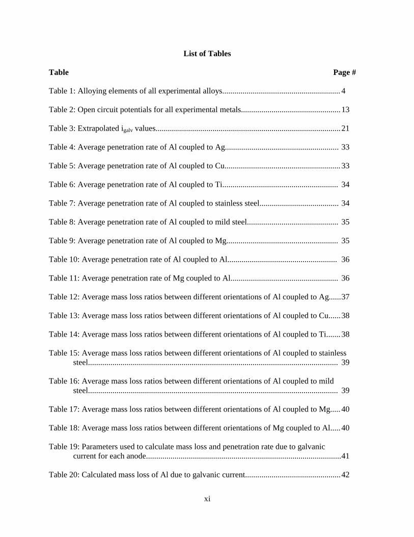
List of Tables

Table Page #

Table 1: Alloying elements of all experimental alloys.......................................................... 4

Table 2: Open circuit potentials for all experimental metals................................................. 13

Table 3: Extrapolated igalv values........................................................................................... 21

Table 4: Average penetration rate of Al coupled to Ag........................................................ 33

Table 5: Average penetration rate of Al coupled to Cu......................................................... 33

Table 6: Average penetration rate of Al coupled to Ti......................................................... 34

Table 7: Average penetration rate of Al coupled to stainless steel....................................... 34

Table 8: Average penetration rate of Al coupled to mild steel............................................. 35

Table 9: Average penetration rate of Al coupled to Mg....................................................... 35

Table 10: Average penetration rate of Al coupled to Al...................................................... 36

Table 11: Average penetration rate of Mg coupled to Al..................................................... 36

Table 12: Average mass loss ratios between different orientations of Al coupled to Ag...... 37

Table 13: Average mass loss ratios between different orientations of Al coupled to Cu...... 38

Table 14: Average mass loss ratios between different orientations of Al coupled to Ti....... 38

Table 15: Average mass loss ratios between different orientations of Al coupled to stainless

steel........................................................................................................................... 39

Table 16: Average mass loss ratios between different orientations of Al coupled to mild

steel........................................................................................................................... 39

Table 17: Average mass loss ratios between different orientations of Al coupled to Mg..... 40

Table 18: Average mass loss ratios between different orientations of Mg coupled to Al..... 40

Table 19: Parameters used to calculate mass loss and penetration rate due to galvanic

current for each anode................................................................................................ 41

Table 20: Calculated mass loss of Al due to galvanic current............................................... 42

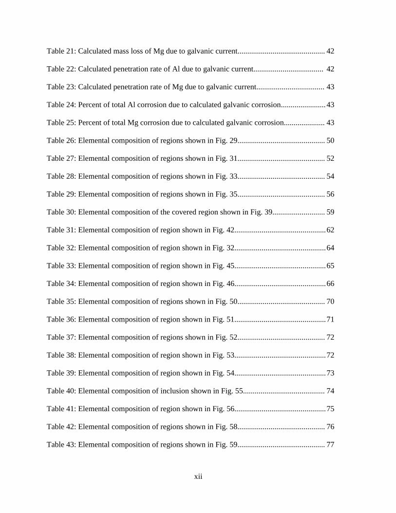
xii

Table 21: Calculated mass loss of Mg due to galvanic current............................................. 42

Table 22: Calculated penetration rate of Al due to galvanic current.................................... 42

Table 23: Calculated penetration rate of Mg due to galvanic current................................... 43

Table 24: Percent of total Al corrosion due to calculated galvanic corrosion....................... 43

Table 25: Percent of total Mg corrosion due to calculated galvanic corrosion..................... 43

Table 26: Elemental composition of regions shown in Fig. 29............................................. 50




Table 30: Elemental composition of the covered region shown in Fig. 39........................... 59

Table 31: Elemental composition of region shown in Fig. 42............................................... 62









Table 40: Elemental composition of inclusion shown in Fig. 55.......................................... 74




xiii





1

Chapter 1: Introduction

Aluminum alloys are used ubiquitously in commercial manufacture and laboratory

applications due to its availability, mechanical properties, light weight, and high corrosion

resistance. The natural passivation of aluminum is a major component in the relatively high

corrosion resistance of aluminum compared to other metals in practical use. However, in

practical use aluminum is commonly used in combination with components of different types of

materials which provide the desired properties. In this research, the aluminum alloy 6061-T6,

one of the most common general-purpose aluminum alloys which contains silicon and

magnesium as its main alloying elements, is analyzed for its corrosion behavior to other

passivating metals (titanium alloy 6Al-4V and 316 stainless steel), non-passivating active metals

(1018 mild steel and magnesium alloy AZ31B), and elemental noble metals (copper and silver).

Aluminum alloy 6061-T6 will henceforth be referred to as Al, titanium alloy 6Al-4V as Ti, 316

stainless steel as stainless steel, 1018 mild steel as mild steel, magnesium alloy AZ31B as Mg,

copper as Cu, and silver as Ag.

1.1.Theory

Galvanic corrosion is a widely researched electrochemical process and is caused by the

flow of current between dissimilar metals in electrical contact.1 In an electrolytic solution, this

current, called galvanic current, electrons flow from the anode to the cathode in the galvanic

couple and thereby increases the corrosion rate of the anode. Local corrosion on the anode also

occurs due to the formation of local cathodic sites on the anode surface. The total corrosion rate

itotal can therefore be summarized as:

itotal = igalv + ilocal (Eq. 1)

2

where igalv is the galvanic component of corrosion and ilocal is the local component of corrosion.

The local corrosion rate ilocal is often estimated as the corrosion rate of an uncoupled metal,

called icorr,uncoupled; however, the effects of the cathodic material may influence ilocal in a manner

unrelated to the galvanic current. Therefore itotal is difficult to predict in practical application

without experimental data.

Fig. 1. Galvanic couple schematic exhibiting galvanic corrosion and local corrosion.

Galvanic corrosion of the anode can be quantified using Faraday’s law, which states that

the amount of species reacted is proportional to the current and the time that the current flowed.2

The mass loss may be calculated using the equation:

(Eq. 2)

where W is the atomic weight of the anode, I is the galvanic current, Δt is the time increment for

each measurement of I, j is number of iterations for the measurements of I, n is the number of

electrons transferred in the half-cell reaction, and F is a Faraday equal to 98,487 Coulombs.

Using the same principle as above, the penetration rate due to galvanic current may also

be calculated using known parameters. The penetration rate (PR) uses several of the same

parameters in (Eq. 2) and follows the equation:

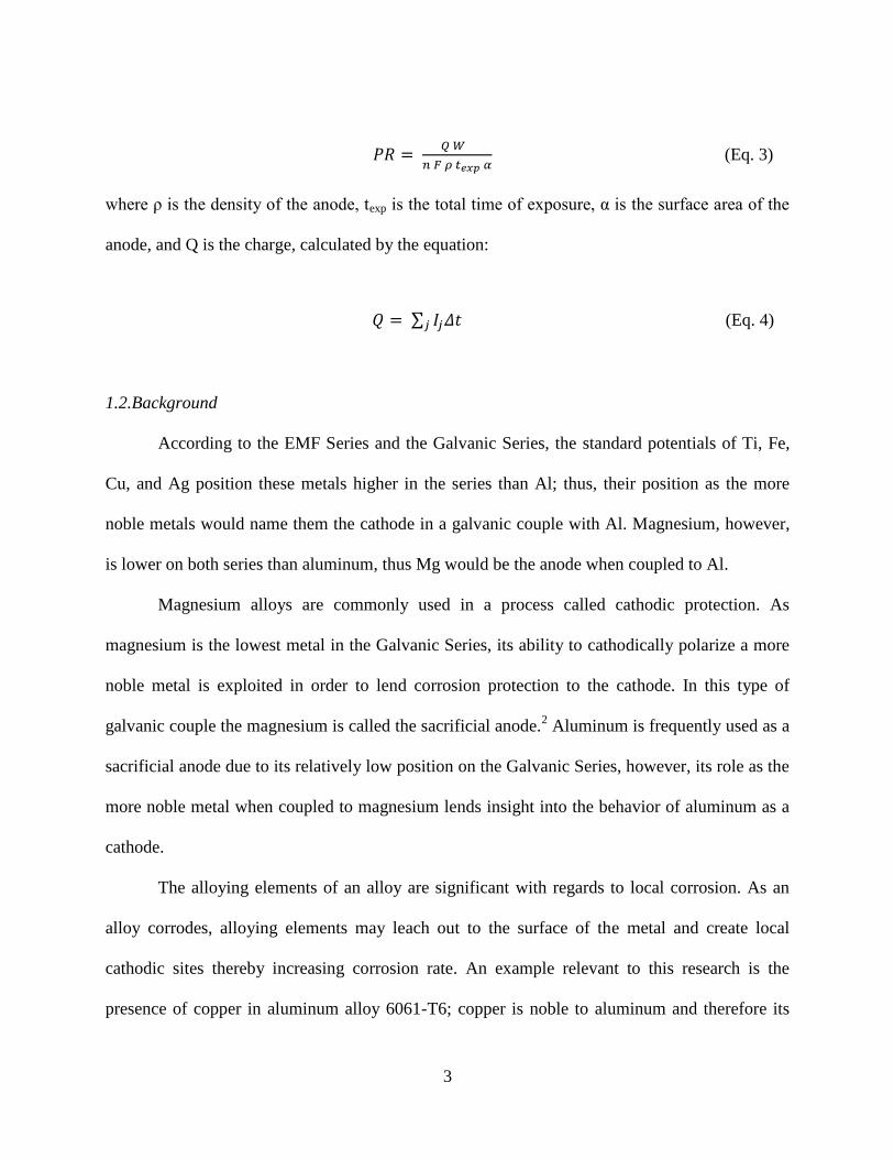
3

(Eq. 3)

where ρ is the density of the anode, texp is the total time of exposure, α is the surface area of the

anode, and Q is the charge, calculated by the equation:

(Eq. 4)

1.2.Background

According to the EMF Series and the Galvanic Series, the standard potentials of Ti, Fe,

Cu, and Ag position these metals higher in the series than Al; thus, their position as the more

noble metals would name them the cathode in a galvanic couple with Al. Magnesium, however,

is lower on both series than aluminum, thus Mg would be the anode when coupled to Al.

Magnesium alloys are commonly used in a process called cathodic protection. As

magnesium is the lowest metal in the Galvanic Series, its ability to cathodically polarize a more

noble metal is exploited in order to lend corrosion protection to the cathode. In this type of

galvanic couple the magnesium is called the sacrificial anode.2 Aluminum is frequently used as a

sacrificial anode due to its relatively low position on the Galvanic Series, however, its role as the

more noble metal when coupled to magnesium lends insight into the behavior of aluminum as a

cathode.

The alloying elements of an alloy are significant with regards to local corrosion. As an

alloy corrodes, alloying elements may leach out to the surface of the metal and create local

cathodic sites thereby increasing corrosion rate. An example relevant to this research is the

presence of copper in aluminum alloy 6061-T6; copper is noble to aluminum and therefore its

4

presence on the surface of the aluminum creates a cathodic site which creates a local action cell

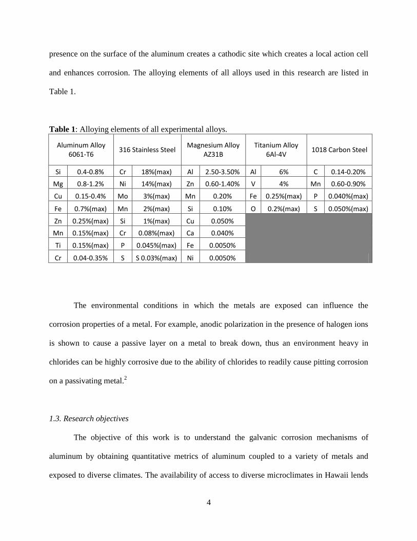
and enhances corrosion. The alloying elements of all alloys used in this research are listed in

Table 1.

Table 1: Alloying elements of all experimental alloys.

Aluminum Alloy 6061-T6

316 Stainless Steel Magnesium Alloy

AZ31B Titanium Alloy

6Al-4V 1018 Carbon Steel

Si 0.4-0.8% Cr 18%(max) Al 2.50-3.50% Al 6% C 0.14-0.20%

Mg 0.8-1.2% Ni 14%(max) Zn 0.60-1.40% V 4% Mn 0.60-0.90%

Cu 0.15-0.4% Mo 3%(max) Mn 0.20% Fe 0.25%(max) P 0.040%(max)

Fe 0.7%(max) Mn 2%(max) Si 0.10% O 0.2%(max) S 0.050%(max)

Zn 0.25%(max) Si 1%(max) Cu 0.050%

Mn 0.15%(max) Cr 0.08%(max) Ca 0.040%

Ti 0.15%(max) P 0.045%(max) Fe 0.0050%

Cr 0.04-0.35% S S 0.03%(max) Ni 0.0050%

The environmental conditions in which the metals are exposed can influence the

corrosion properties of a metal. For example, anodic polarization in the presence of halogen ions

is shown to cause a passive layer on a metal to break down, thus an environment heavy in

chlorides can be highly corrosive due to the ability of chlorides to readily cause pitting corrosion

on a passivating metal.2

1.3. Research objectives

The objective of this work is to understand the galvanic corrosion mechanisms of

aluminum by obtaining quantitative metrics of aluminum coupled to a variety of metals and

exposed to diverse climates. The availability of access to diverse microclimates in Hawaii lends

5

an opportunity to gain a comprehensive view of the corrosion properties in varying corrosive

environments. For this reason the experimental test sites included a marine environment at

Marine Corps Base Hawaii (MCBH), a rainforest environment at Lyon Arboretum, a volcanic

environment at Kilauea Volcanoes National Park, and in a cyclic corrosion testing chamber

subjected to a standardized accelerated corrosion test in the laboratory to simulate outdoor

exposure. The large variety of commonly used alloys were selected for this research in order to

provide the most practical insight into aluminum-coupled metals and provide data for future

modeling of galvanic corrosion of aluminum.

Experimental techniques employed in order to predict galvanic corrosion behavior of

aluminum included potentiodynamic polarization to generate mixed-potential plots, and

observation of pH change of galvanically-coupled aluminum in a solid electrolyte. Analytical

techniques following laboratory and field exposure of the corroded galvanic couples included

standardized cleaning in order to obtain mass loss data, calculations of mass loss and penetration

rate due to galvanic corrosion using (Eq. 2) and (Eq. 3) based on Faraday’s law, and surface

analysis techniques including Scanning Electron Microscopy (SEM) in combination with Energy

Dispersive X-ray Analysis (EDXA) and X-ray Diffraction (XRD).

6

Chapter 2: Literature Review

2.1. Pitting corrosion of aluminum

The innate corrosion resistance of aluminum due to its ability to passivate is often

reduced by pitting corrosion. Numerous studies have been performed on the effect of chloride

ions on pitting corrosion.2-7

A study by McCafferty describes the sequence of pitting on

aluminum by chloride ions, in which the chloride ions adsorb onto the oxide surface and

penetrate the passive oxide film, dissolve the aluminum, and propagate by rupture of blisters

formed at the metal surface.4 Another study on pitting corrosion of aluminum by Szklarska-

Smialowska, the author describes the adsorption of chloride ions on the passive film. Szklarska-

Smialowska discusses the heterogeneity of the metal surface, which caused a variation in the

adsorption of chloride ions to the passive film.5 A study by Blanc and Mankowski also describes

the pitting corrosion on aluminum alloy 6056 as being partially attributed to the heterogeneous

passive film due to the alloy’s intermetallic particles.6

While chloride ions are known to initiate and propagate pitting corrosion, other ions have

been found to suppress corrosion. In a study by Datta, Bhattacharya, and Bandyopadhyay, the

effect of Cl-, Br

-, NO

3-, and SO4

2- on aluminum alloy 6061 were examined; it was found that

while Cl- increased pitting corrosion, NO3-

and Br- were less corrosive and SO4

2- seemed to

increase the passivity of the alloy, further reducing the pitting corrosion of the alloy.7 The

aforementioned study by Szklarska-Smialowska also makes note that the addition of sulfate to

the chlorides introduced to the aluminum slowed the chloride adsorption, albeit without ceasing

chloride uptake. 5

The susceptibility of 6*** series aluminum alloys to pitting corrosion is of particular

interest for this research. In the previously mentioned study by Blanc and Mankowski, the

7

authors found that aluminum alloy 6056 was more susceptible to pitting corrosion than

aluminum alloy 2024 for lower chloride ion concentrations, while the 2024 alloy was much more

susceptible in high chloride ion concentrations.6 Similarly in a study by Dan, Muto and Hara,

aluminum alloy 6061 experienced more rapidly increasing pitting than aluminum alloy 1100

until a chloride-deposition rate of 100 mg m-2

day-1

was reached, at which the pitting of the 1100

alloy increased with increased chloride deposition and the pitting of the 6061 alloy decreased

with pitting corrosion rate.8 These data are significant in a study involving aluminum alloy 6061

so that the corrosion behavior of the alloy may be well-understood.

2.2. Atmospheric corrosion of aluminum alloys

The corrosion behavior of aluminum and aluminum alloys in an atmospheric study is

invaluable due to the marked difference in laboratory-induced results versus field results.

Atmospheric corrosion data is potentially more representative of corrosion in practical settings.

Previous atmospheric corrosion studies of aluminum includes a study by Cui et al. wherein

aluminum alloy 7A04 was exposed in a tropical marine atmosphere for four years; one

significant finding in this study was that corrosion rate actually slowed long-term due to the

buildup of corrosion product over the surface of the metal.9 Another study by Ezuber, El-houd,

and El-Shawesh examined the corrosion of aluminum alloys 5083 and 1100 in natural seawater.

One conclusion of this study was that Al12Fe3Si2 particles as well as Mg in the alloy were greatly

susceptible to pitting corrosion when exposed to sea water.10

These findings are also pertinent

regarding aluminum alloy 6061, as it contains both Al-Fe-Si inclusions and also contains Mg as

one of its major alloying elements.

8

2.3. Galvanic corrosion of aluminum-coupled metals

Previous studies of galvanically-coupled aluminum and aluminum alloys have been

surveyed for those involving the metals used in this research. In a similar yet smaller-scale study

by Acevedo-Hurtado et al., aluminum alloy 2024 was galvanically coupled to commercially pure

Ag and exposed in a tropical marine environment as well as in accelerated corrosion tests ASTM

B117 and GM-9540P. The authors findings included pitting corrosion of the aluminum alloy

with increased corrosion in the crevice, as well as uniform corrosion on the Ag, albeit minimal

Ag corrosion due to protective film formation and galvanic protection. The authors also found

that sulfate and oxide deposits inhibit pit nucleation.11

Galvanic corrosion of commercially pure iron and aluminum in NaCl solution was

studied by Raj and Nishimura wherein a scanning electrochemical microscope (SECM) was used

to determine the sacrificial behavior of aluminum as the anode in the couple. A drop in potential

over time was detected by the SECM tip and the concentration of oxygen decreased due to

oxygen reduction on the iron.12

A study by Rafla et al. of aluminum alloy 7050 coupled to 304 stainless steel in a

simulated fastener under droplets of NaCl solution. After 62 hours of NaCl exposure multiple

fissures were revealed in the aluminum alloy in the region surrounding the stainless steel wire.

These fissures were likely due to both the cathodic action of the stainless steel as well as local

cathodic sites inherent in the aluminum alloy.13

An atmospheric study of an Al-Cu galvanic couple in a marine environment performed

by Vera, Verdugo, Orellana, and Muñoz identified pitting corrosion and exfoliation of the

aluminum when coupled to copper as well as crevice corrosion in the lap joint due to galvanic

9

action. The aluminum corrosion was increased in the presence of environmental copper and

sulfur dioxide.14

In a study of pure aluminum coupled to pure magnesium by Lacroix, Blanc, Pébère,

Tribollet, and Vivier, an increase in both the aluminum and the magnesium in the study was

observed. Their findings stated that although aluminum is the cathode in an Al-Mg galvanic

couple, the dissolution of Mg generating hydroxide ions subsequently led to an increase in pH in

the Na2SO4 solution in which the couple was immersed, which aided in the degradation of the Al

passive layer and thus increased corrosion in both species.15

Literature was scarce on galvanic corrosion studies of aluminum coupled to titanium,

however a theoretical model study of Al coupled to Ti by Younan, Zhiqiang, Siping, and Hao

was developed with the goal of mitigating galvanic corrosion on microchip bond pads. The

authors proposed solutions to bond pad corrosion based on known reactions of aluminum and

titanium corrosion, such as eliminating moisture to prevent oxygen reduction and maintaining

aluminum passivation to slow corrosion.16

10

Chapter 3: Preliminary Experiments

3.1. Observation of pH change in galvanic couples

One indication of galvanic corrosion is the change in pH on either side of the galvanic

cell. As galvanic current passes from the cathode to anode in the presence of an electrolytic

solution, the reduction at the cathode facilitates the oxygen reduction reaction, generating

hydroxide ions and increasing the pH of the environment surrounding the cathode.

Simultaneously, the oxidation of the anode generates metal cations that become hydrated thereby

generating hydrogen ions and decreasing the pH of the environment surrounding the anode. This

principle is particularly significant in the corrosion of the anode, as the buildup of H+ ions

attracts the anions of the electrolyte solution; the increased presence of aggressive anions (e.g.

Cl-) in the region surrounding the anode may further accelerate corrosion. An experiment was

conducted in order to visually observe this effect in the galvanic couple types to be researched in

this work.

Galvanic couples consisting of Al-Ag, Al-Cu, Al-Ti, Al-stainless steel, Al-mild steel, and

Al-Mg were assembled with non-conductive fasteners. A molten agar electrolyte at neutral pH

consisting of 3.15 wt% NaCl and a pH indicator solution containing phenolphthalein,

bromthymol blue, methyl orange, alizarine yellow R, bromocresol green, and meta cresol purple

was poured around each galvanic couple until the couples were enclosed in the solution. The

specimens were then left undisturbed to allow for cooling and solidification of the agar and

stored in the laboratory at 20°C. Observations were conducted over the 48 hours following the

experimental setup.

Gas formation on the Mg side of the Al-Mg galvanic couple was visually apparent

immediately (Fig. 2a). Upon addition of the electrolyte to the dish containing the Al-Mg couple,

11

bubbling of the solution indicated what was likely hydrogen evolution on the Mg surface.

However, based on the extreme susceptibility of magnesium to hydrogen evolution, this

observed effect may not be entirely attributed to the galvanic corrosion mechanism.2 In addition

to the immediate hydrogen evolution reaction a slight color change in the agar surrounding the

Al coupon in the Al-Mg couple was visible.

Over a period of 4 hours, the dark purple color change of the electrolyte surrounding the

Al coupon in the Al-Mg couple indicated a significant increase in alkalinity compared to the

local area around the Mg (Fig. 2b). Slight light orange color change indicating acidity around the

Al coupons of the Al-stainless steel and the Al-mild steel couples was also observed after 4 hours

in the solid electrolyte. Gas formation for all couples was indicated by bubble formation in the

agar, likely due to hydrogen formation at the cathodic sites.

After 24 hours, color differentials on the Al-Ag, Al-stainless steel, and the Al-mild steel

couples were observed, demarking the anodic region and the cathodic regions wherein the Al

side was anodic and the corresponding metal side was cathodic (Fig. 2c). After 48 hours all

galvanic couples displayed gas formation and a pH change in the local environment, albeit less

pronounced in the Al-Cu and Al-Ti couples.

ssdf a) b)

12

Fig. 2. Galvanic couples of (left to right, 1

st row) Al-Cu, Al-stainless steel, Al-Mg, and (left to

right, 2nd

row) Al-Ag, Al-Ti, and Al-mild steel after a) 0 hours (5-minutes exposure), b) 4 hours,

c)12 hours, d) 24 hours, e) 36 hours, and f) 48 hours.

3.2. Potentiodynamic polarization

Potentiodynamic polarization experiments were performed using the Parstat 2273

Advanced Potentiostat with 1-cm. x 1-cm. electrodes in aerated solutions of 3.15 wt% NaCl and

0.5 M Na2SO4 against a Saturated Calomel Electrode (SCE) with KCl. First, open-circuit

potentials (OCP) were obtained over a one-hour period for Al, Ag, Cu, Ti, stainless steel, and

mild steel, and over a 30-minute period for Mg. The aerated solutions were sparged with air at a

volumetric rate of 320-370 mL/min at a pressure of 1 atm. This rate was held constant for all of

c) d)

e) f)

13

the polarization tests. The average OCP values for each metal in the NaCl and Na2SO4 solutions

are displayed in Table 2.

Table 2: Open circuit potentials for all experimental metals.

Metal Average OCP in aerated

3.15 wt% NaCl (V vs. SCE) Average OCP in aerated 0.5 M Na2SO4 (V vs. SCE)

AA6061-T6 -0.790 -0.482

Silver -0.0880 0.0943

Copper -0.253 -0.0722

Ti 6Al-4V -0.459 -0.303

316 Stainless Steel -0.148 -0.221

1018 Mild Steel -0.582 -0.628

Mg AZ31B -1.60 -1.60

The OCP values of Al, Ag, Cu, Ti, stainless steel, and mild steel in NaCl indicate these

metals as the cathode when coupled to Al, as the Al has a lower potential than all values listed

for the aforementioned metals. However, in Na2SO4 solution the OCP for mild steel was higher

than that of Al. This indicates that in an Al-mild steel galvanic couple, the designation of the

anode and cathode may switch depending on the ions in the surrounding environment. Al has a

higher potential than Mg in both solutions, indicating Al as the cathode in both cases.

The OCP values for Al, Ag, Cu, Ti, were lower in NaCl solution than in Na2SO4 solution

while the stainless steel and mild steel displayed lower OCP values in the Na2SO4 solution than

in the NaCl solution.

Thus, in NaCl solution cathodic polarization curves for Ag, Cu, Ti, stainless steel, and

mild steel were obtained, and anodic polarization curves for Mg were obtained (Figs. 3-8). In

Na2SO4 solution, cathodic polarization curves for Ag, Cu, Ti, and stainless steel were obtained,

as well as anodic polarization curves for mild steel and Mg (Figs. 9-14). These polarization

14

curves were overlain with the corresponding anodic or cathodic curve for Al. Figs. 15 and 16

display overlays of all polarization curves obtained in NaCl and Na2SO4 solution, respectively.

Fig. 3. Cathodic Ag and anodic Al polarization in 3.15 wt% NaCl solution.

Fig. 4. Cathodic Cu and anodic Al polarization in 3.15 wt% NaCl solution.

15

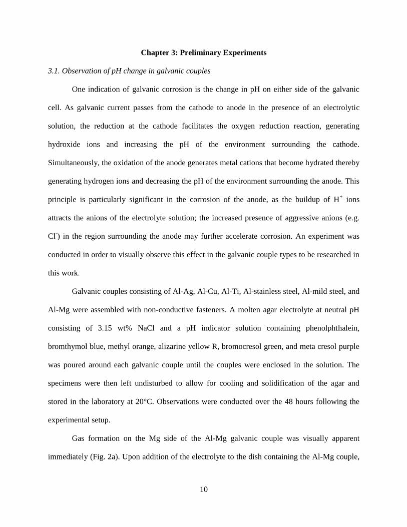
Fig. 5. Cathodic Ti and anodic Al polarization in 3.15 wt% NaCl solution.

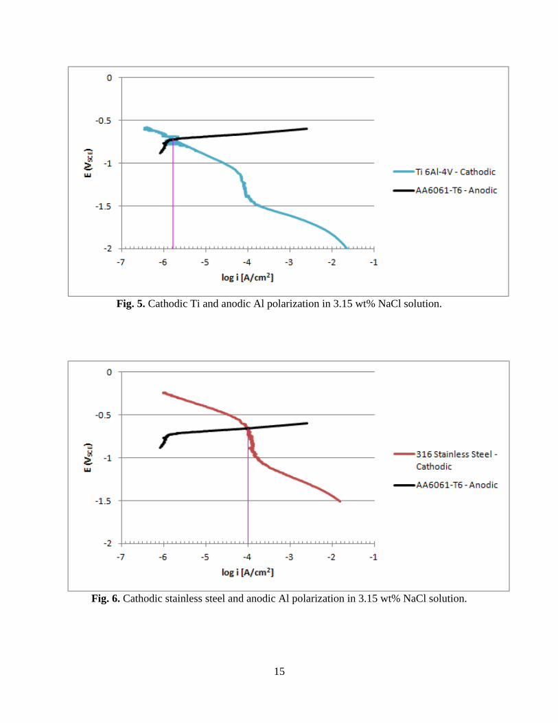
Fig. 6. Cathodic stainless steel and anodic Al polarization in 3.15 wt% NaCl solution.

16

Fig. 7. Cathodic mild steel and anodic Al polarization in 3.15 wt% NaCl solution.

Fig. 8. Cathodic Al and anodic Mg polarization in 3.15 wt% NaCl solution.

17

Fig. 9. Cathodic Ag and anodic Al polarization in 0.5 M Na2SO4 solution.

Fig. 10. Cathodic Cu and anodic Al polarization in 0.5 M Na2SO4 solution.

18

Fig. 11. Cathodic Ti and anodic Al polarization in 0.5 M Na2SO4 solution.

Fig. 12. Cathodic stainless steel and anodic Al polarization in 0.5 M Na2SO4 solution.

19

Fig. 13. Cathodic Al and anodic mild steel polarization in 0.5 M Na2SO4 solution.

Fig. 14. Cathodic Al and anodic Mg polarization in 0.5 M Na2SO4 solution.

20

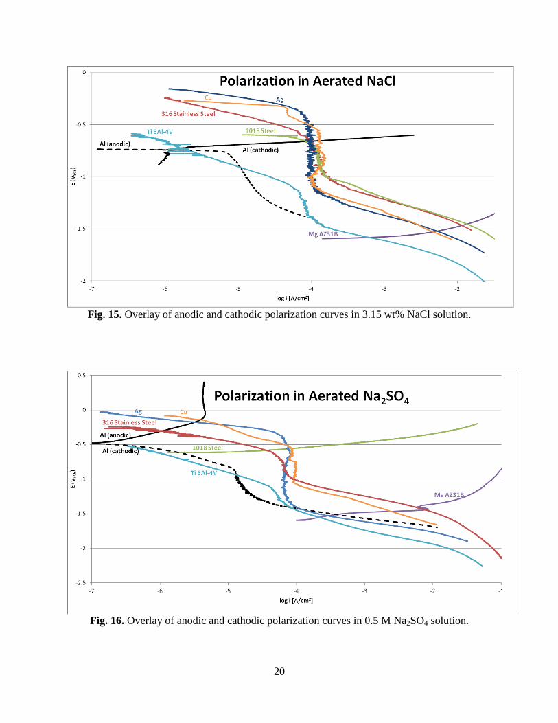
Fig. 15. Overlay of anodic and cathodic polarization curves in 3.15 wt% NaCl solution.

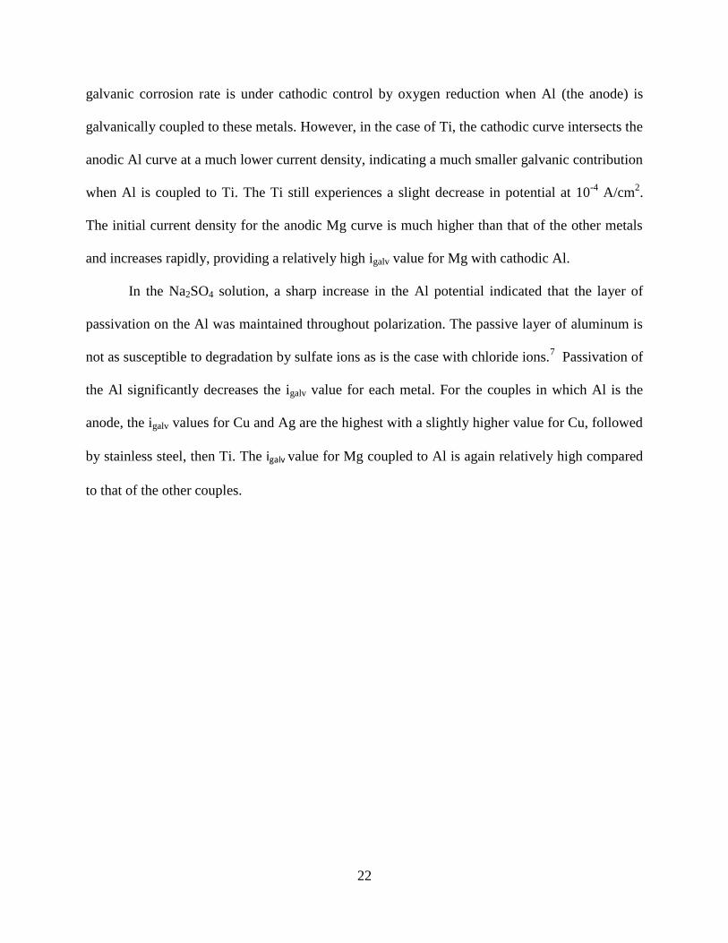
Fig. 16. Overlay of anodic and cathodic polarization curves in 0.5 M Na2SO4 solution.

21

The point of intersection of the anodic and cathodic curve of each metal type represents

the galvanic current (igalv), or the contribution of galvanic current to galvanic corrosion of the

anode.1 The extrapolated igalv values for each metal coupled to Al in NaCl solution and Na2SO4

solution are listed in Table 3.

Table 3: Extrapolated igalv values.

Metal log igalv [A/cm2] in 3.15 wt% NaCl log igalv [A/cm2] in 0.5 M Na2SO4

Ag -4.0 -5.5

Cu -3.9 -5.4

Ti -5.8 -6.7

Stainless Steel -4.0 -6.0

Mild Steel -4.1 -5.7*

Mg -2.5* -3.4*

*The log igalv values represent the galvanic contribution of aluminum to these metals, as

aluminum is indicated as the cathode when coupled to these metals in the presence of the stated

electrolyte.

In the NaCl solution, the anodic Al curve shows a rapid increase in current density at

around 10-6

A/cm2, indicating a breakdown of the passive film on the Al surface. Most cathodic

curves experience a sharp decrease in potential around a current density of 10-4

A/cm2 which is

the diffusion-limited oxygen reduction current density in the polarization cell. Oxygen reduction

is often the primary cathodic reaction when metals corrode in aerated solutions.2 Mg is an

exception where the predominant cathodic reaction is hydrogen evolution in both aerated and

deaerated solutions. It is around the diffusion-limited oxygen reduction current density that igalv

is obtained for Ag, Cu, stainless steel, and mild steel, with a slightly higher current density value

for Cu. This may have been due to slight fluctuation in the air sparge rate or more active cathodic

sites on the copper versus the other metals. The polarization behavior of the metals indicated the

22

galvanic corrosion rate is under cathodic control by oxygen reduction when Al (the anode) is

galvanically coupled to these metals. However, in the case of Ti, the cathodic curve intersects the

anodic Al curve at a much lower current density, indicating a much smaller galvanic contribution

when Al is coupled to Ti. The Ti still experiences a slight decrease in potential at 10-4

A/cm2.

The initial current density for the anodic Mg curve is much higher than that of the other metals

and increases rapidly, providing a relatively high igalv value for Mg with cathodic Al.

In the Na2SO4 solution, a sharp increase in the Al potential indicated that the layer of

passivation on the Al was maintained throughout polarization. The passive layer of aluminum is

not as susceptible to degradation by sulfate ions as is the case with chloride ions.7 Passivation of

the Al significantly decreases the igalv value for each metal. For the couples in which Al is the

anode, the igalv values for Cu and Ag are the highest with a slightly higher value for Cu, followed

by stainless steel, then Ti. The igalv value for Mg coupled to Al is again relatively high compared

to that of the other couples.

23

Chapter 4: Experimental Procedures for Environmental Exposure

4.1. Galvanic couple specimen assembly

Couples were assembled using 2-in. x 1-in. coupons of Ag, Cu, Ti, stainless steel, mild

steel, and Mg mechanically coupled to 2-in. x 1-in. Al coupons using non-conductive, glass-

reinforced polyurethane fasteners tightened to the maximum working torque of 10 in.-lbs. A non-

conductive sheet of G10 fiberglass was inserted between the metals in all couples for which

galvanic current was to be measured; couples that were not being measured for galvanic

corrosion did not contain the insulating sheet and were included in the experiment in

quadruplicate. Non-coupled coupons of each metal were also included in the experiment in

quadruplicate. Non-conductive, inert insulators and fasteners were used to mount the coupled

and uncoupled metals onto powder-coated aluminum face plates.

Fig. 17. Assembled galvanic couple a) Schematic b) Assembled and mounted Al-Cu couple pre-

environmental exposure

4.2. Support system

The galvanic couples and corresponding uncoupled metals were grouped by metal type

and mounted on their designated face plate and position. The face plates were separated by

acrylic barriers to prevent cross-contamination and were then mounted onto fiberglass struts

(Fig. 19). The entire unit was then placed flat (0-degree angle from the horizontal) onto the test

rack.

a) b)

24

Fig. 18. Face plate containing Al-Cu galvanic couples and uncoupled Cu.

Fig. 19. Illustration of support system.

4.3. Data logger configuration

Galvanic current was measured using differential voltage loggers and resistors. Triplicate

couples of each type were connected to either a Madgetech QuadVolt, a Madgetech OctVolt, or a

Madgetech Volt101A voltage data logger via TCL 4-wire cables and epoxied weather-resistant

connectors. Resistor magnitude was 1 Ω for the samples in the cyclic corrosion testing chamber

(CCTC) and 10 Ω for the outdoor exposure tests. Data loggers were kept in a water resistant,

lockable enclosure fortified with desiccant. With the preparation of an extra set of data loggers

25

and a color-coded cable joint system, the logger sets were able to be readily exchanged at the test

site with minimal data loss to allow for data downloading and logger inspection in the laboratory.

Fig. 20. Wiring schematic of voltage data loggers.

Fig. 21. Top view of enclosed data loggers. Fig. 22. Color-coded cable joints outside

of logger box.

26

4.4. Specimen exposure

Four sets of experimental galvanic couples and uncoupled metals were assembled and

deployed to four different testing sites for environmental exposure. These sites included the

CCTC, MCBH, Kilauea, and Lyon Arboretum (Fig. 23).

Fig. 23. Experimental specimens at a) CCTC, b) MCBH, c) Kilauea, d) Lyon Arboretum.

The specimens in the CCTC were subjected to the experimental conditions standardized

in the GM-9540P accelerated corrosion test. A single modification was made in the angle of

placement of the specimens which was set at 0 degrees from the horizontal. A cycle of the GM-

9540P test is 24 hours long and involves a series of salt solution spray containing NaCl, CaCl2,

and NaHCO3 at room temperature, followed by a period of 100% relative humidity at 49°C, and

a) b)

c) d)

27

finally a dry-off period of high heat at 60°C (Figure 24). The specimens were exposed in the

CCTC for 30 cycles. Voltage data was logged every 1 minute and was downloaded roughly once

a week throughout the exposure period.

Fig. 24. Environmental conditions of the GM-9540P accelerated corrosion test. Courtesy of

Daniel P. Schmidt of Army Research Office.

a) b)

28

Fig. 25. Galvanic couples following four cycles of the GM-9540P test consisting of a) Al and

Ag, b) Al and stainless steel, c) Al and mild steel, d) Al and Mg, e) Al and Ti, and f) Al and Cu.

The outdoor exposure specimens were deployed for a period of 4 months. Voltage data

was logged every 5 minutes and was downloaded roughly once a month, wherein the voltage

logger box was disconnected and exchanged throughout each outdoor test site. The experimental

specimens themselves were undisturbed by laboratory members during each data logger box

exchange. Figs. 26-28 show the galvanic couples at each test site following one month exposure.

All specimens were returned to the laboratory and removed from the support mounts

following exposure. The couples were disassembled and separated for analysis.

c) d)

e) f)

29

Fig. 26. Galvanic couples after one month of exposure at MCBH consisting of a) Al and Ag, b)

Al and stainless steel, c) Al and mild steel, d) Al and Mg, e) Al and Ti, and f) Al and Cu.

a) b)

c) d)

e) f)

30

Fig. 27. Galvanic couples after one month of exposure at Kilauea consisting of a) Al and Ag, b)

Al and stainless steel, c) Al and mild steel, d) Al and Mg, e) Al and Ti, and f) Al and Cu.

a) b)

c) d)

e) f)

31

Fig. 28. Galvanic couples after one month of exposure at Lyon Arboretum consisting of a) Al

and Ag, b) Al and stainless steel, c) Al and mild steel, d) Al and Mg, e) Al and Ti, and f) Al and

Cu.

a) b)

c) d)

e) f)

32

Chapter 5: Determination of Corrosion Rate

5.1. Penetration rate and mass loss

The corroded Al coupons were subjected to a chemical cleaning procedure for corrosion

product removal in order to determine the total mass loss of the specimens. The Al cleaning

solution consisted of 2% chromium trioxide and 5% phosphoric acid following International

Standard ISO 8407: 1991 (E) C.1.1. Because Mg is anodic to Al in the Al-Mg galvanic couple,

the mass loss of Mg was also of interest. The Mg coupons were also subjected to corrosion

product removal and cleaned in a solution containing 20% chromium trioxide, 2% barium

nitrate, and 1% silver nitrate following the standard ASTM G1 C.5.2 cleaning procedure. The

final mass of each cleaned specimen was recorded and subtracted from the initial mass to

determine the total mass loss.

The average penetration rate was calculated for the uncoupled Al and each position of

coupled Al (i.e. Al-on-top or X-on-top position where X is the corresponding Al-coupled metal)

at each exposure site. The penetration rate of the coupled Al were further separated by the set of

Al couples with a voltage data logger attached and the set of those without a logger attached. The

test samples subjected to exposure in the CCTC included two sets of galvanic couples attached to

data loggers in both the Al-on-top and X-on-top orientation; all couples attached to data loggers

at the outdoor exposure sites (i.e. MCBH, Lyon Arboretum [LA], and Kilauea [KIL]) were in the

X-on-top orientation only. All sites contained sets of galvanic couples without a data logger

attached in both orientations. The average penetration rates for each set of exposed Al are listed

in Tables 4-9.

33

Table 4: Average penetration rate of Al coupled to Ag in mm per year.

Exposure site

Uncoupled

Coupled with logger Coupled without logger Al on top

Ag on top

Al on top

Ag on top

CCTC 2.73E-02 4.46E-01 5.39E-01 3.08E-01 2.38E-01

MCBH 6.27E-04

6.42E-02 5.74E-02 4.55E-02

LA 2.13E-04 9.89E-03 2.46E-02 2.16E-02

KIL 8.28E-04 8.57E-03 1.86E-02 1.66E-02

Table 5: Average penetration rate of Al coupled to Cu in mm per year.

Exposure site

Uncoupled


Cu on top

Al on top

Cu on top

CCTC 2.73E-02 4.56E-01 5.58E-01 4.39E-01 4.38E-01

MCBH 6.27E-04

5.52E-02 7.45E-02 6.71E-02

LA 2.13E-04 7.37E-03 2.42E-02 2.05E-02

KIL 8.28E-04 7.19E-03 1.74E-02 1.85E-02

34

Table 6: Average penetration rate of Al coupled to Ti in mm per year.

Exposure site

Uncoupled


Ti on top

Al on top

Ti on top

CCTC 2.73E-02 4.65E-02 4.38E-02 2.91E-02 3.32E-02

MCBH 6.27E-04

1.40E-02 6.20E-03 9.57E-03

LA 2.13E-04 1.76E-03 3.52E-03 1.67E-03

KIL 8.28E-04 1.74E-03 2.71E-03 2.41E-03

Table 7: Average penetration rate of Al coupled to stainless steel in mm per year.

Exposure site

Uncoupled


Stainless steel on top

Al on top


CCTC 2.73E-02 2.33E-01 2.63E-01 1.34E-01 8.16E-02

MCBH 6.27E-04

2.04E-02 2.78E-02 2.03E-02

LA 2.13E-04 5.22E-03 7.76E-03 5.61E-03

KIL 8.28E-04 3.77E-03 2.41E-03 2.88E-03

35

Table 8: Average penetration rate of Al coupled to mild steel in mm per year.

Exposure site

Uncoupled


Mild steel on top

Al on top

Mild steel on top

CCTC 2.73E-02 6.41E-01 4.26E-01 2.13E-01 2.33E-01

MCBH 6.27E-04

4.01E-02 4.10E-02 5.03E-02

LA 2.13E-04 7.77E-03 1.58E-02 1.44E-02

KIL 8.28E-04 1.54E-02 9.71E-03 1.18E-02

Table 9: Average penetration rate of Al coupled to Mg in mm per year.

Exposure site

Uncoupled


Mg on top

Al on top

Mg on top

CCTC 2.73E-02 6.07E-02 7.97E-02 6.14E-02 1.51E-01

MCBH 6.27E-04

2.89E-03 4.81E-03 5.51E-03

LA 2.13E-04 5.91E-04 5.68E-04 6.27E-04

KIL 8.28E-04 5.28E-04 4.44E-04 4.56E-04

36

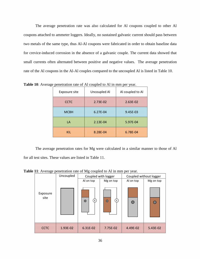
The average penetration rate was also calculated for Al coupons coupled to other Al

coupons attached to ammeter loggers. Ideally, no sustained galvanic current should pass between

two metals of the same type, thus Al-Al coupons were fabricated in order to obtain baseline data

for crevice-induced corrosion in the absence of a galvanic couple. The current data showed that

small currents often alternated between positive and negative values. The average penetration

rate of the Al coupons in the Al-Al couples compared to the uncoupled Al is listed in Table 10.

Table 10: Average penetration rate of Al coupled to Al in mm per year.

Exposure site Uncoupled Al Al coupled to Al

CCTC 2.73E-02 2.63E-02

MCBH 6.27E-04 9.45E-03

LA 2.13E-04 5.97E-04

KIL 8.28E-04 6.78E-04

The average penetration rates for Mg were calculated in a similar manner to those of Al

for all test sites. These values are listed in Table 11.

Table 11: Average penetration rate of Mg coupled to Al in mm per year.

Exposure site

Uncoupled


Mg on top

Al on top

Mg on top

CCTC 1.93E-02 6.31E-02 7.75E-02 4.49E-02 5.43E-02

37

MCBH 5.58E-02

9.65E-02 6.88E-02 7.59E-02

LA 3.38E-02 4.14E-02 3.24E-02 3.98E-02

KIL 2.73E-02 3.33E-02 2.29E-02 3.24E-02

In viewing the average penetration rate data, it is apparent that the corrosion rate differed

depending on the orientation in which the Al was exposed, even among Al coupled to the same

type of metal. In addition to the mass loss percentages, the ratios of average mass loss were

calculated between each orientation of exposed Al; the ratios include the coupled Al with logger

to the uncoupled Al, the coupled Al without logger to the uncoupled Al, and the coupled Al with

logger to the coupled Al without logger. For the latter ratios in which both compared sets are

coupled Al, the ratio was calculated with the corresponding Al-on-top or X-on-top orientation.

Calculated ratios are listed in Tables 12-17.

Table 12: Average mass loss ratios between different orientations of Al coupled to Ag.

Exposure site

Coupled Al w/ logger to Uncoupled Al

Coupled Al w/o logger to Uncoupled Al

Coupled Al w/ logger to Coupled Al w/o logger

Al on top

Ag on top

Al on top

Ag on top

Al on top

Ag on top

CCTC 16.3 19.7 11.3 8.73 1.45 2.26

MCBH

102. 92.0 72.7

1.41

LA 46.4 115. 101. 0.459

KIL 10.3 22.4 20.0 0.516

38

Table 13: Average mass loss ratios between different orientations of Al coupled to Cu.

Exposure

site




Al on top

Cu on top

Al on top

Cu on top

Al on top

Cu on top

CCTC 16.7 20.5 16.1 16.0 1.04 1.28

MCBH

88.1 119. 107.

0.823

LA 34.6 114. 96.5 0.356

KIL 8.68 21.0 22.3 0.389

Table 14: Average mass loss ratios different orientations of Al coupled to Ti.

Exposure site




Al on top

Ti on top

Al on top

Ti on top

Al on top

Ti on top

CCTC 1.70 1.60 1.07 1.22 1.60 1.32

MCBH

22.3 9.89 15.3

1.46

LA 8.28 16.6 7.83 1.06

KIL 2.10 3.28 2.91 0.721

39

Table 15: Average mass loss ratios between different orientations of Al coupled to stainless

steel.

Exposure site




Al on top


Al on top


Al on top


CCTC 8.54 9.62 4.91 2.99 1.74 3.22

MCBH

32.6 44.3 32.4

1.01

LA 24.5 36.4 26.3 0.930

KIL 4.55 2.91 3.48 1.31

Table 16: Average mass loss ratios different orientations of Al coupled to mild steel.

Exposure site




Al on top

Mild steel on top

Al on top

Mild steel on top

Al on top

Mild steel on top

CCTC 23.5 15.6 7.79 8.53 3.01 1.83

MCBH

64.1 65.4 80.3

0.798

LA 36.5 74.4 67.8 0.538

KIL 18.7 11.7 14.2 1.31

40

Table 17: Average mass loss ratios between different orientations of Al coupled to Mg.

Exposure site




Al on top

Mg on top

Al on top

Mg on top

Al on top

Mg on top

CCTC 2.22 2.92 2.25 5.54 0.988 0.527

MCBH

4.60 7.68 8.79

0.524

LA 2.78 2.67 2.94 0.943

KIL 0.638 0.536 0.551 1.16

The average mass loss ratios for Mg were calculated in a similar manner to those of Al

for all test sites. These values are listed in Table 18.

Table 18: Average mass loss ratios between different orientations of Mg coupled to Al.

Exposure site

Coupled Mg w/ logger to Uncoupled Mg

Coupled Mg w/o logger to Uncoupled Mg

Coupled Mg w/ logger to Coupled Mg w/o logger

Al on top

Mg on top

Al on top

Mg on top

Al on top

Mg on top

CCTC 3.27 4.02 2.33 2.82 1.41 1.43

MCBH

1.73 1.23 1.36

1.27

LA 1.23 0.960 1.18 1.04

KIL 1.22 0.837 1.18 1.03

41

5.2. Galvanic corrosion rate

Mass loss and penetration rate of the anode due to galvanic current were calculated using

(Eq. 2) and (Eq. 3). The voltage values recorded using the data loggers and the known resistance

values were used to calculate the summation of galvanic current. The parameters used to

calculate mass loss and penetration rate due to galvanic current are as listed in Table 19.

Table 19: Parameters used to calculate mass loss and penetration rate due to galvanic current for

each anode.

Al Mg

n 3 2

W [g/mole] 27 24.305

α [cm2] 28.22575 28.22575

g/cm3 2.7 1.74

texp,CCTC [days] 30 30

texp,KIL [days] 133 133

texp,LA/MCBH [days] 135 135

RCCTC [Ω] 1 1

Routdoor [Ω] 10 10

The logged voltage for Al coupled to Ag, Cu, Ti, stainless steel, and mild steel was

positive for all test sites and negative when coupled to Mg at all test sites. Thus, the galvanic

mass loss δm was calculated for Al coupled to Ag, Cu, Ti, stainless steel, and mild steel; the

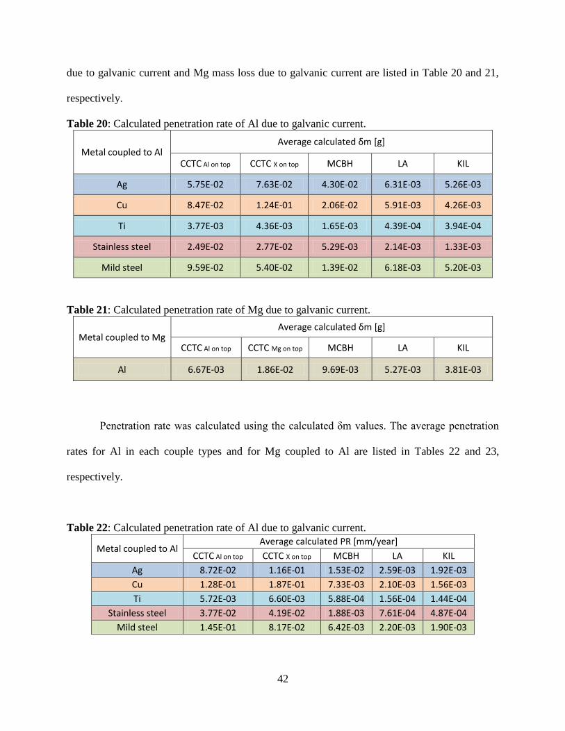
galvanic mass loss was calculated for Mg coupled to Al. The calculated values for Al mass loss

42

due to galvanic current and Mg mass loss due to galvanic current are listed in Table 20 and 21,

respectively.

Table 20: Calculated penetration rate of Al due to galvanic current.

Metal coupled to Al Average calculated δm [g]

CCTC Al on top CCTC X on top MCBH LA KIL

Ag 5.75E-02 7.63E-02 4.30E-02 6.31E-03 5.26E-03

Cu 8.47E-02 1.24E-01 2.06E-02 5.91E-03 4.26E-03

Ti 3.77E-03 4.36E-03 1.65E-03 4.39E-04 3.94E-04

Stainless steel 2.49E-02 2.77E-02 5.29E-03 2.14E-03 1.33E-03

Mild steel 9.59E-02 5.40E-02 1.39E-02 6.18E-03 5.20E-03

Table 21: Calculated penetration rate of Mg due to galvanic current.

Metal coupled to Mg Average calculated δm [g]

CCTC Al on top CCTC Mg on top MCBH LA KIL

Al 6.67E-03 1.86E-02 9.69E-03 5.27E-03 3.81E-03

Penetration rate was calculated using the calculated δm values. The average penetration

rates for Al in each couple types and for Mg coupled to Al are listed in Tables 22 and 23,

respectively.

Table 22: Calculated penetration rate of Al due to galvanic current.

Metal coupled to Al Average calculated PR [mm/year]


Ag 8.72E-02 1.16E-01 1.53E-02 2.59E-03 1.92E-03

Cu 1.28E-01 1.87E-01 7.33E-03 2.10E-03 1.56E-03

Ti 5.72E-03 6.60E-03 5.88E-04 1.56E-04 1.44E-04

Stainless steel 3.77E-02 4.19E-02 1.88E-03 7.61E-04 4.87E-04

Mild steel 1.45E-01 8.17E-02 6.42E-03 2.20E-03 1.90E-03

43

Table 23: Calculated penetration rate of Mg due to galvanic current.

Metal coupled to Mg Average calculated PR [mm/year]


Al 1.57E-02 4.37E-02 5.35E-03 2.91E-03 2.16E-03

In order to quantify the galvanic corrosion rate in terms of the total corrosion rate, the

penetration rate due to galvanic current was calculated as a percentage of the total mass loss of

the coupon post-exposure; in other words, this value is the contribution of galvanic corrosion to

total corrosion. These values are listed in Table 24 and 25 for Al corrosion and Mg corrosion,

respectively.

Table 24: Percent of total Al corrosion due to calculated galvanic corrosion.

Metal coupled to Al Average % of total corrosion due to galvanic corrosion


Ag 19.5% 21.5% 23.8% 26.2% 22.4%

Cu 28.2% 33.5% 13.3% 28.5% 21.7%

Ti 12.3% 15.1% 4.21% 8.85% 8.26%

Stainless steel 16.2% 16.0% 9.22% 14.6% 12.9%

Mild steel 22.7% 19.2% 16.0% 28.3% 12.3%

Table 25: Percent of total Mg corrosion due to calculated galvanic corrosion.

Metal coupled to Mg Average % of total corrosion due to galvanic corrosion


Al 24.8% 56.5% 5.54% 7.02% 6.48%

44

5.3. Discussion of corrosion rate

Average penetration rate was nearly universally higher for samples exposed in the CCTC.

The direct and regular administration of the salt spray to the test specimens in the CCTC was

likely the case of the vastly accelerated corrosion, and was not a factor present in the outdoor test

sites which relied on uncontrolled environmental conditions. The environment in which most

couples corroded at the second highest rate was at MCBH. The marine environment mimics the

accelerated corrosion test performed in the CCTC most closely due to the presence of

atmospheric chlorides and other salts found in seawater and the surrounding ocean front. In

general, the couples experienced the third highest amount of corrosion in the rainforest

environment at Lyon Arboretum, followed lastly by the volcanic environment at Kilauea. The

combination of regular rainfall and high humidity at Lyon Arboretum likely contributed to the

higher corrosion rate of Al than at Kilauea; however, both sites produced relatively low

corrosion rates than the Al specimens in the CCTC and at MCBH.

The total corrosion was generally highest in Al when coupled to either Ag or Cu, with

slightly more corrosion when coupled to Ag at the CCTC and MCBH sites, and roughly the same

amount of corrosion when coupled to either Ag or Cu at the Lyon Arboretum and Kilauea sites.

The next most corroded set of Al is the Al which was coupled to mild steel, followed by stainless

steel, then Ti, and lastly Mg. Although stainless steel and Ti are both passivating metals, Al

when coupled to stainless steel corroded two to three times the amount as those coupled to Ti at

every test site except for Kilauea, where the Al only corroded slightly higher when coupled to

stainless steel than to Ti. Notable exceptions to the stated order of corrosion by coupled metal are

the Al samples coupled to either mild steel or Mg in the CCTC. The Al coupled to mild steel and

attached to data loggers in the Al-on-top orientation had a higher mass loss percentage than the

Al coupled to Ag and Cu in the same orientation. Additionally, all Al samples coupled to Mg had

45

a higher mass loss percentage than the Al coupled to Ti, which for the other test sites showed a

higher corrosion rate than those coupled to Mg. A possible explanation for the increased

corrosion in Al coupled to mild steel and Mg is their location in the CCTC—these particular

specimens were positioned adjacent to each other and directly under a nozzle in which the salt

spray was deployed; thus, these particular specimens likely received a larger amount of salt spray

than other specimens in the chamber leading to further accelerated corrosion.

The total corrosion percentage of the uncoupled Al at all outdoor test sites was minimal

at less than 0.05%, thus the difference in the average mass loss between all uncoupled aluminum

exposed in the outdoor test sites is taken to be negligible. However, the average mass loss

percentage of uncoupled Al in the CCTC was much higher than in the outdoor sites at 0.316%.

This is likely again due to the direct administration of salt spray to the Al, which subjects the

passive layer on the Al to attack, lowering the passivity and increasing corrosion rate. In the

outdoor field exposure, the airborne ions were insufficient to appreciably degrade the passive

layer on the uncoupled Al as compared those exposed in the CCTC.

Amount of corrosion was relatively equal in the Al coupled to another Al coupon

compared to the uncoupled Al, with one exception in the Al coupled to Al at MCBH which

corroded at a considerably higher rate (i.e., 15.1 times higher) than the uncoupled Al at the same

site. Because both metals in the couple were of the same type, this single increase in corrosion

cannot be attributed to galvanic corrosion. One possible explanation could be the presence of a

crevice in the Al coupled to Al—the interface between the Al coupons creates an anoxic

environment wherein crevice corrosion may occur leading to breakdown of the passive layer and

propagation of the corrosion by chloride ion attack.

46

The Mg specimens coupled to Al generally corroded at a higher rate at each site than the

uncoupled Mg, except in the case of Lyon Arboretum and Kilauea for the specimens in the Al-

on-top orientation where corrosion was actually less when coupled than uncoupled; these

exceptions were likely due to these specimens’ position in which protection of half the top

surface of the Mg coupon was lent by the Al coupon. Interestingly, the Mg experienced more

corrosion overall at MCBH than in the CCTC. A possible explanation for this is that since Mg

does not have the passivating ability as Al does, the chlorides present in the atmosphere at

MCBH initiated corrosion of Mg immediately and was sustained for the four-month duration of

exposure. Since the chloride concentration at MCBH is so high, the Mg specimens never dry out

due to the hygroscopic properties of the chloride deposits. In the CCTC, the specimens are in the

dry-cycle for 1/3 of the exposure time. Also, since Mg corrodes by hydrogen evolution rather

than oxygen reduction, the second phase of the GM-9540P test that induces high diffusion-

limited oxygen reduction rates due to the formation of a thin electrolyte layer at 100% RH does

not enhance the rate of Mg corrosion.

The mass loss ratios highlight the differences in Al corrosion depending on the manner in

which it was exposed. Al corrosion was considerably higher when coupled to another metal

versus the uncoupled Al, with the lowest ratios ranging from 1.07-20.5 times the corrosion in the

CCTC and the highest ratios ranging from 15.3-119 times the corrosion at MCBH. The low

ratios from the Al samples in the CCTC may again be attributed to the higher corrosion overall

of the uncoupled Al in the CCTC compared to the other sites. The only scenario in which the Al

ratio was lower than one for the coupled Al to the uncoupled Al was in coupling with Mg at

Kilauea. In these coupled samples, corrosion rate actually decreased compared to the uncoupled

47

Al, suggesting that the Al coupons not only retained their passive layer but were afforded

cathodic protection from Mg.

The ratios between coupled Al with the logger attached to the coupled Al without the

logger attached were calculated due to the presence of the electrically insulating sheet between

the metals in the couples attached to the logger. There was no noticeable trend in these ratios

across the Al couples corresponding to each metal; however, for the Ag-Al and Cu-Al couples at

Lyon Arboretum and Kilauea, the Al without the logger attached corroded at a higher rate than

the Al with the logger attached. These two sites yielded the lowest corrosion rates, yet the

highest amount of corrosion that occurred at these sites was for the Al specimens in direct

contact with the noble active metals.

The ratios for Mg are less dramatic than those of Al. The general trend was that coupled

Mg corroded more than uncoupled Mg with some exceptions in the couples where Al was

positioned on top of the Mg in the less corrosive environments. The ratio of coupled Mg with a

logger attached to coupled Mg without a logger showed that more Mg corrosion occurred when

attached to a logger and in direct contact with the Al at the CCTC and MCBH sites, and close to

equal at Lyon Arboretum and Kilauea. For the Mg samples in direct contact with the Al,

corrosion products in the interface can electrically decouple the Mg from the Al and break the

galvanic couple, which is likely more pronounced in the CCTC and at MCBH where corrosion

rates were higher. The samples connected to the logger are electrically connected through the

wire leads and hence, the galvanic couple cannot be broken for the entire exposure period.

The mass loss data and ratios clearly display that Al in a galvanic couple corrodes more

than uncoupled Al, and similarly with Mg in a couple versus uncoupled. However, the

contribution of galvanic current to corrosion was a small fraction in most cases to the total

48

corrosion of the specimen. With the exception of one set of Al coupled to Cu in the CCTC, all

calculated galvanic components of corrosion were less than 30% of the total corrosion that was

determined by mass loss. Furthermore, for all Al coupled to Ti or stainless steel, the galvanic

component made up less than 20% of the total corrosion. Thus, the total corrosion could not have

been quantified using the calculated mass loss due to the galvanic current in addition to the

amount of local corrosion on the uncoupled Al. As previously stated, crevice corrosion could

account for the increase in Al corrosion when coupled to another metal. Another explanation is

the local contamination of the Al by the coupled metal—ions from the cathodic metal may

transfer to the surface of the Al and create local cathodic sites which would induce corrosion.

These processes may lead to accelerated corrosion wherein the alloying elements of the Al may

be exposed, creating cathodic sites due to its own composition. In addition, the separation of the

cathode and anode can lead to enhanced alkalinity on the cathodic metal and enhanced acidity on

and chloride migration to the anodic metal, leading to accelerated corrosion.

The calculated galvanic contribution to total Mg corrosion was considerably higher in the

CCTC than in the outdoor field sites, with 24.8% and 56.5% of total corrosion due to galvanic

current in the CCTC and less than 8% contribution for all outdoor sites. Accordingly, in the

outdoor field sites there was no extreme difference in corrosion of Mg in a couple versus

uncoupled Mg, whereas the galvanically-coupled Mg in the CCTC corroded between two to four

times as much as the uncoupled Mg depending on its orientation. Thus, the discrepancy in the

contribution of galvanic current may be due to the samples in the CCTC being in continuous

electrical contact throughout the one-month exposure period; whereas, in the four-month outdoor

exposure period, contact between the two metals was possibly weakly maintained due to severe

corrosion over time.

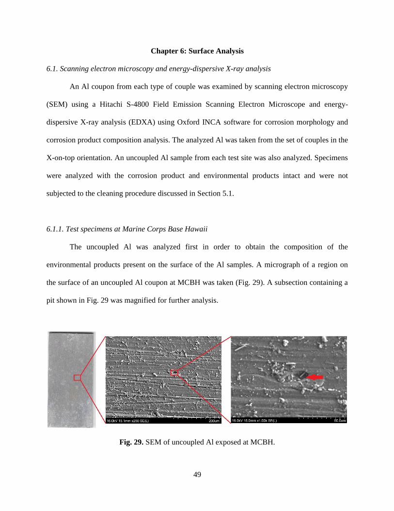
49

Chapter 6: Surface Analysis

6.1. Scanning electron microscopy and energy-dispersive X-ray analysis

An Al coupon from each type of couple was examined by scanning electron microscopy

(SEM) using a Hitachi S-4800 Field Emission Scanning Electron Microscope and energy-

dispersive X-ray analysis (EDXA) using Oxford INCA software for corrosion morphology and

corrosion product composition analysis. The analyzed Al was taken from the set of couples in the

X-on-top orientation. An uncoupled Al sample from each test site was also analyzed. Specimens

were analyzed with the corrosion product and environmental products intact and were not

subjected to the cleaning procedure discussed in Section 5.1.

6.1.1. Test specimens at Marine Corps Base Hawaii

The uncoupled Al was analyzed first in order to obtain the composition of the

environmental products present on the surface of the Al samples. A micrograph of a region on

the surface of an uncoupled Al coupon at MCBH was taken (Fig. 29). A subsection containing a

pit shown in Fig. 29 was magnified for further analysis.

Fig. 29. SEM of uncoupled Al exposed at MCBH.

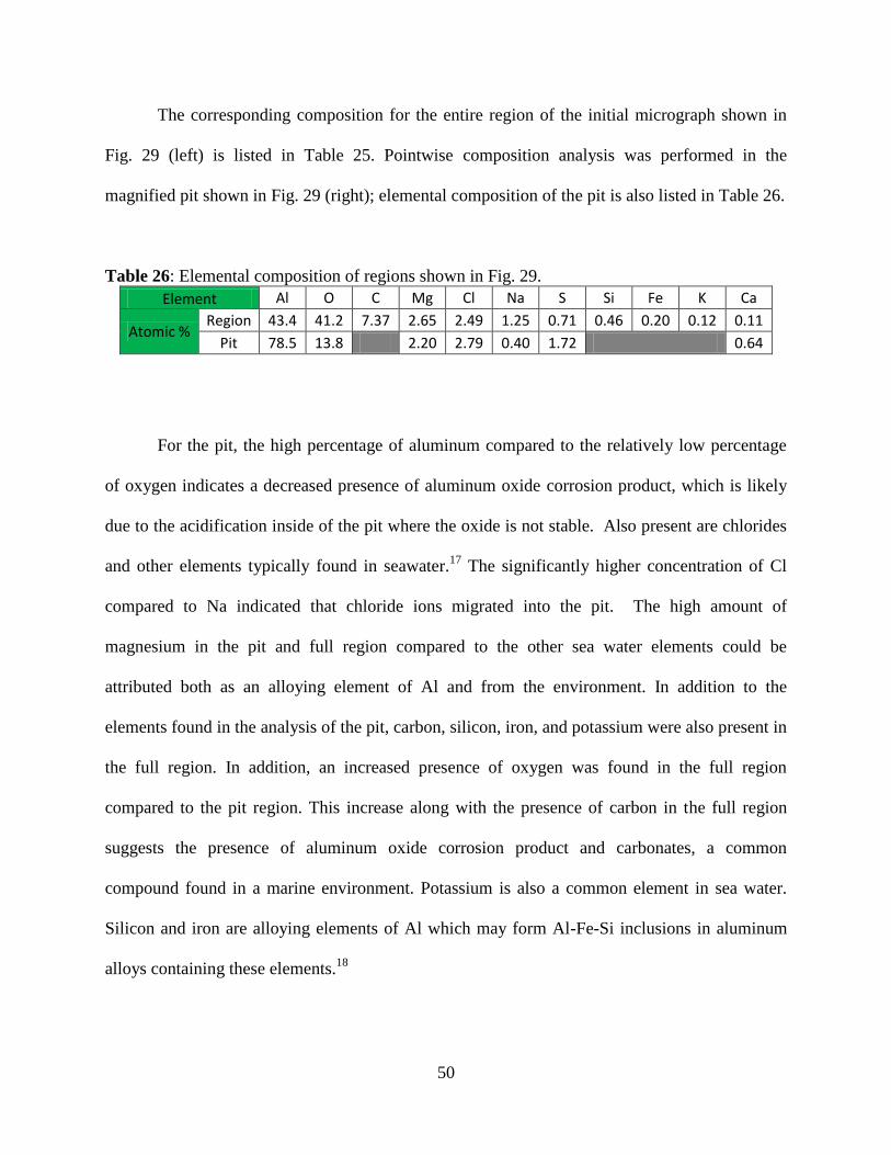
50

The corresponding composition for the entire region of the initial micrograph shown in

Fig. 29 (left) is listed in Table 25. Pointwise composition analysis was performed in the

magnified pit shown in Fig. 29 (right); elemental composition of the pit is also listed in Table 26.

Table 26: Elemental composition of regions shown in Fig. 29.

Element Al O C Mg Cl Na S Si Fe K Ca

Atomic % Region 43.4 41.2 7.37 2.65 2.49 1.25 0.71 0.46 0.20 0.12 0.11

Pit 78.5 13.8 2.20 2.79 0.40 1.72 0.64

For the pit, the high percentage of aluminum compared to the relatively low percentage

of oxygen indicates a decreased presence of aluminum oxide corrosion product, which is likely

due to the acidification inside of the pit where the oxide is not stable. Also present are chlorides

and other elements typically found in seawater.17

The significantly higher concentration of Cl

compared to Na indicated that chloride ions migrated into the pit. The high amount of

magnesium in the pit and full region compared to the other sea water elements could be

attributed both as an alloying element of Al and from the environment. In addition to the

elements found in the analysis of the pit, carbon, silicon, iron, and potassium were also present in

the full region. In addition, an increased presence of oxygen was found in the full region

compared to the pit region. This increase along with the presence of carbon in the full region

suggests the presence of aluminum oxide corrosion product and carbonates, a common

compound found in a marine environment. Potassium is also a common element in sea water.

Silicon and iron are alloying elements of Al which may form Al-Fe-Si inclusions in aluminum

alloys containing these elements.18

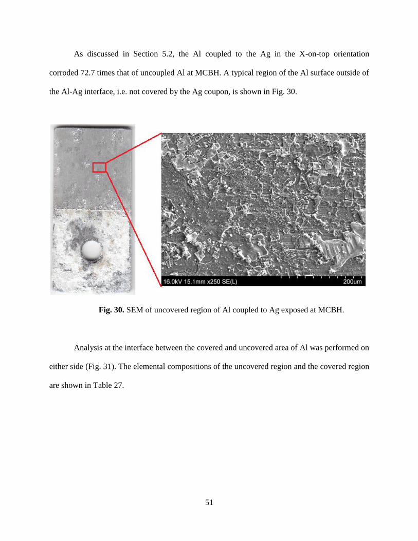
51

As discussed in Section 5.2, the Al coupled to the Ag in the X-on-top orientation

corroded 72.7 times that of uncoupled Al at MCBH. A typical region of the Al surface outside of

the Al-Ag interface, i.e. not covered by the Ag coupon, is shown in Fig. 30.

Fig. 30. SEM of uncovered region of Al coupled to Ag exposed at MCBH.

Analysis at the interface between the covered and uncovered area of Al was performed on

either side (Fig. 31). The elemental compositions of the uncovered region and the covered region

are shown in Table 27.

52

Fig. 31. SEM of interface between covered (top right) and uncovered (bottom right) regions of

Al coupled to Ag at MCBH.


Element O Al C Mg Cl Na S Ca Ag Si Fe K

Atomic %

Covered 70.1 13.0 6.42 6.42 1.7 1.25 0.63 0.62 0.16

Uncovered 72.1 9.87 10.1 2.40 1.79 0.78 0.70 1.50 0.73 0.11

For the uncovered region, the iron and silicon included in the composition analysis suggests that

the Al oxide corrosion product did not completely shield the alloying elements. Oxygen was the

most abundant element, primarily due to the formation of aluminum oxide. For the covered

region, the presence of silver was detected in addition to the other common elements. This may

be attributed to contamination of the Al by Ag which likely accelerated the corrosion of the Al

coupon.

53

The sample that experienced the most corrosion at MCBH was the Al that was coupled to

Cu. A typical region on the uncovered surface of Al coupled to Cu is shown in Fig. 32. An

abundance of salt particles are visible in the micrograph; however, corrosion of the Al surface is

less severe than that of the Al coupled to Ag.

Fig. 32. SEM of uncovered region of Al coupled to Cu exposed at MCBH.

Compositional analysis was performed on the thick layer of product on the Al coupon in

the region covered by Cu. Visual inspection indicates that elemental transfer from the Cu coupon

occurred. A micrograph was taken of a typical part of this region (Fig. 33) and compositional

analysis was performed in three areas: 1) the entire area of the micrograph, 2) pointwise on one

of the spheres shown in the top region of the micrograph, and 3) pointwise on the thick crust

layer on the bottom right of the micrograph. The results of this analysis are shown in Table 28.

54

Fig. 33. SEM of covered region of Al coupled to Cu exposed at MCBH.


Element O Al C Mg Na Cu Cl Ca S

Atomic %

1 Region 68.5 12.4 9.55 4.09 1.47 2.06 1.01 0.51 0.47

2 Sphere 64.4 0.86 17.4 17.3

3 Crust 57.5 5.57 10.7 3.19 22.5 0.56

The analysis of the entire area shown in the micrograph is similar to that of the covered area of

the Al coupled to Ag, with a notable exception that the presence of copper was detected instead

of Ag. This also suggests that copper was deposited onto the surface of the Al and accelerated

corrosion in this region. A pointwise analysis of one of the spheres shown in the micrograph

identifies this as calcium carbonate. In the third analysis, the atomic percentage of copper

increased significantly to 22.5%, indicating that some regions of the Al coupon were

contaminated by the Cu coupon more heavily than others.

55

The Al coupon coupled to Ti corroded the least amount of all couples in which Al was

the anode. The micrograph of the longitudinal end of the uncovered surface of Al shows minimal

corrosion in addition to typical salt deposits (Fig. 34).

Fig. 34. SEM of uncovered region of Al coupled to Ti exposed at MCBH.

The uncovered surface of the Al coupled to stainless steel showed a surface morphology

that was less corroded than that of Al coupled to Cu (Fig. 35). The surface analysis of the whole

region shown in Fig. 35 (left SEM) did not show any atypical results. However, the dark flat

deposits were magnified and examined in more detail.

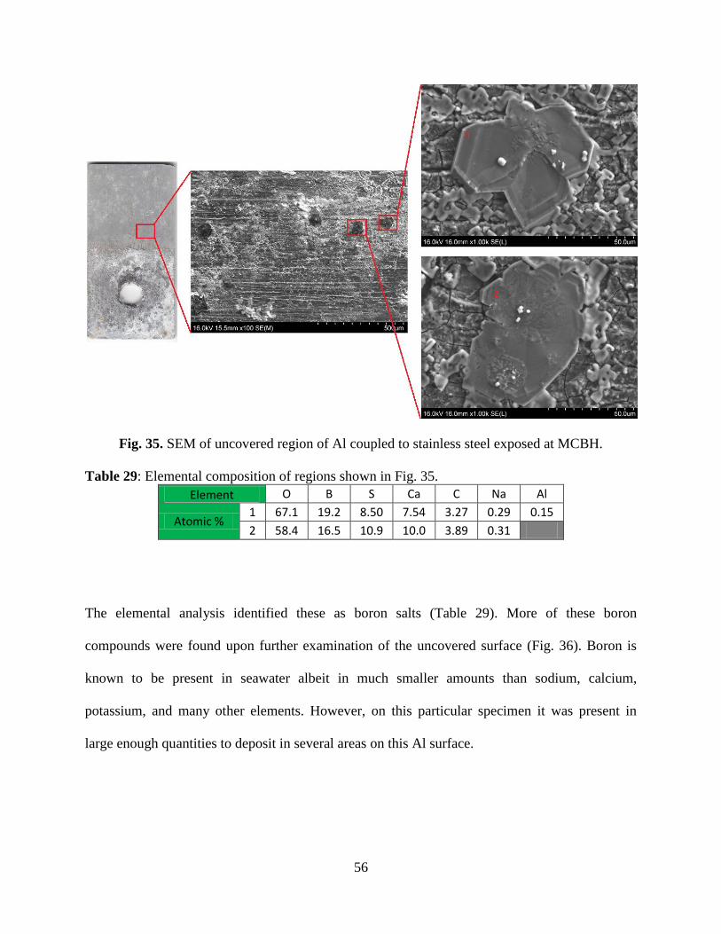
56

Fig. 35. SEM of uncovered region of Al coupled to stainless steel exposed at MCBH.


Element O B S Ca C Na Al

Atomic % 1 67.1 19.2 8.50 7.54 3.27 0.29 0.15

2 58.4 16.5 10.9 10.0 3.89 0.31

The elemental analysis identified these as boron salts (Table 29). More of these boron

compounds were found upon further examination of the uncovered surface (Fig. 36). Boron is

known to be present in seawater albeit in much smaller amounts than sodium, calcium,

potassium, and many other elements. However, on this particular specimen it was present in

large enough quantities to deposit in several areas on this Al surface.

57

Fig. 36. SEM of boron salts found on Al coupled to stainless steel at MCBH.

The region of Al covered by stainless steel was also examined for corrosion morphology.

Since stainless steels are extremely susceptible to crevice corrosion, the propagation of crevice

corrosion in the interface of the two coupons could facilitate crevice corrosion on the Al as well.

Fig. 37 is a micrograph of a region around the hole in the Al through which the fastener was

placed. This region shows degradation of the passive layer on the Al surface.

Fig. 37. SEM of covered region of Al coupled to stainless steel near the crevice mouth exposed

at MCBH.

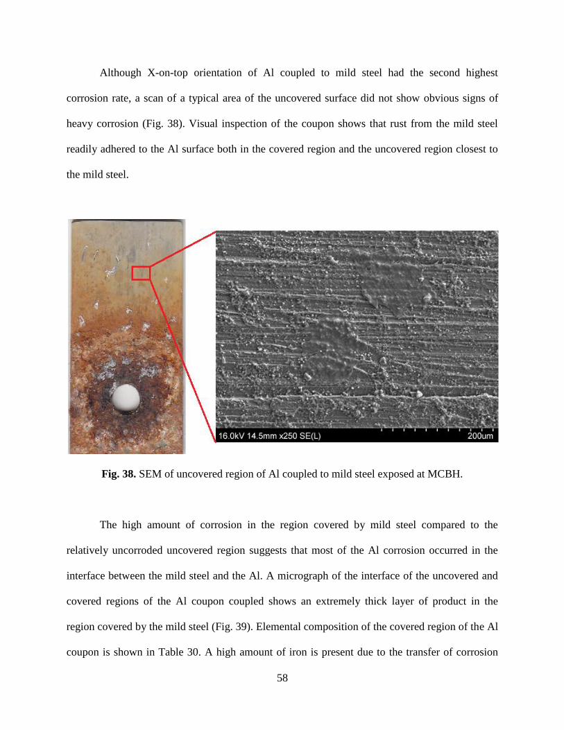
58

Although X-on-top orientation of Al coupled to mild steel had the second highest

corrosion rate, a scan of a typical area of the uncovered surface did not show obvious signs of

heavy corrosion (Fig. 38). Visual inspection of the coupon shows that rust from the mild steel

readily adhered to the Al surface both in the covered region and the uncovered region closest to

the mild steel.

Fig. 38. SEM of uncovered region of Al coupled to mild steel exposed at MCBH.

The high amount of corrosion in the region covered by mild steel compared to the

relatively uncorroded uncovered region suggests that most of the Al corrosion occurred in the

interface between the mild steel and the Al. A micrograph of the interface of the uncovered and

covered regions of the Al coupon coupled shows an extremely thick layer of product in the

region covered by the mild steel (Fig. 39). Elemental composition of the covered region of the Al

coupon is shown in Table 30. A high amount of iron is present due to the transfer of corrosion

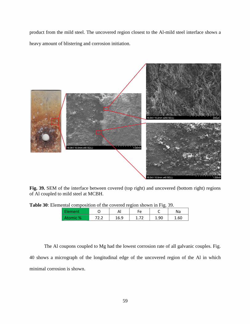
59

product from the mild steel. The uncovered region closest to the Al-mild steel interface shows a

heavy amount of blistering and corrosion initiation.

Fig. 39. SEM of the interface between covered (top right) and uncovered (bottom right) regions

of Al coupled to mild steel at MCBH.

Table 30: Elemental composition of the covered region shown in Fig. 39.

Element O Al Fe C Na

Atomic % 72.2 16.9 1.72 1.90 1.60

The Al coupons coupled to Mg had the lowest corrosion rate of all galvanic couples. Fig.

40 shows a micrograph of the longitudinal edge of the uncovered region of the Al in which

minimal corrosion is shown.

60

Fig. 40. SEM of uncovered region of Al coupled to Mg exposed at MCBH.

Most of the Al corrosion occurred in the interface of the two metals where Al was

covered. Fig. 41 compares the difference in corrosion morphology in this interfacial region for

the Al coupled to Mg, which had the lowest corrosion rate, compared to the Al coupled to Ag,

which had a relatively high corrosion rate.

61

Fig. 41. SEM comparison of corrosion in covered regions of Al coupled to Mg (top) and Al

coupled to Ag (bottom) exposed at MCBH.

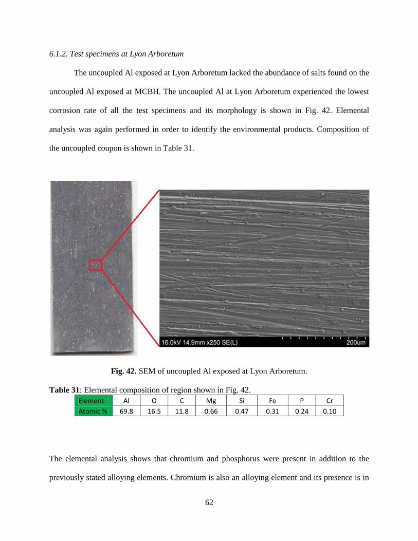
62

6.1.2. Test specimens at Lyon Arboretum

The uncoupled Al exposed at Lyon Arboretum lacked the abundance of salts found on the

uncoupled Al exposed at MCBH. The uncoupled Al at Lyon Arboretum experienced the lowest

corrosion rate of all the test specimens and its morphology is shown in Fig. 42. Elemental

analysis was again performed in order to identify the environmental products. Composition of

the uncoupled coupon is shown in Table 31.

Fig. 42. SEM of uncoupled Al exposed at Lyon Arboretum.

Table 31: Elemental composition of region shown in Fig. 42.

Element Al O C Mg Si Fe P Cr

Atomic % 69.8 16.5 11.8 0.66 0.47 0.31 0.24 0.10

The elemental analysis shows that chromium and phosphorus were present in addition to the

previously stated alloying elements. Chromium is also an alloying element and its presence is in

63

accordance with the composition of the alloy. The presence of phosphorous may be attributed to

rain water or organic life found in the rainforest environment.

Al coupled to Ag at Lyon Arboretum had the highest corrosion rate at this test site;

however, the corrosion rate was still much lower than that of the chloride-heavy environments

(MCBH and in the CCTC). A micrograph of the uncovered surface of Al coupled to Mg is

shown in Fig. 43.

Fig. 43. SEM of uncovered region of Al coupled to Ag exposed at Lyon Arboretum.

Inspection for corroded areas of the uncovered region of the Al coupled to Cu were

discovered and magnified to 1000x. Elemental analysis was performed in one such region where

cracking of the oxide layer was apparent (Fig. 44). The composition of this region is shown in

Table 32.

64

Fig. 44. SEM of surface cracking on the uncovered region of Al coupled to Cu at Lyon

Arboretum.


Element Al O C Mg Si S Fe P Cu

Atomic % 51.9 37.4 9.25 0.49 0.41 0.27 0.13 0.10 0.06

The composition includes copper though in such small quantities that its presence may be

attributed to the composition of the Al alloy.

The presence of copper in the covered crevice region of the Al coupon was again visually

apparent. Elemental analysis of the region covered by the Cu coupon confirms the presence of

copper (Fig. 45 and Table 33).

65

Fig. 45. SEM of covered region of Al coupled to Cu exposed at Lyon Arboretum.


Element O Al C Cu Mg Si

Atomic % 75.2 19.8 4.10 0.41 0.34 0.11

The corrosion product from the mild steel was again present on the surface of the Al to

which it was coupled. Composition of an area of the covered region of Al close to the fastener

hole (Fig. 46) is listed in Table 34.

66

Fig. 46. SEM of covered region of Al coupled to mild steel exposed at Lyon Arboretum.


Element O Fe Al C Mn

Atomic % 62.6 19.0 14.40 3.60 0.36

Iron was present in large amounts as expected. Manganese was also discovered in the analysis.

Although manganese is an alloying element of Al, the amount present was higher than the

composition of the alloy. The mild steel also contains Mn as an alloying element.

The Al with the lowest corrosion rates at Lyon Arboretum, i.e. those coupled to Ti,

stainless steel, and Mg (Figs. 47-49), showed minimal signs of corrosion and no elements

previously unseen during compositional analysis.

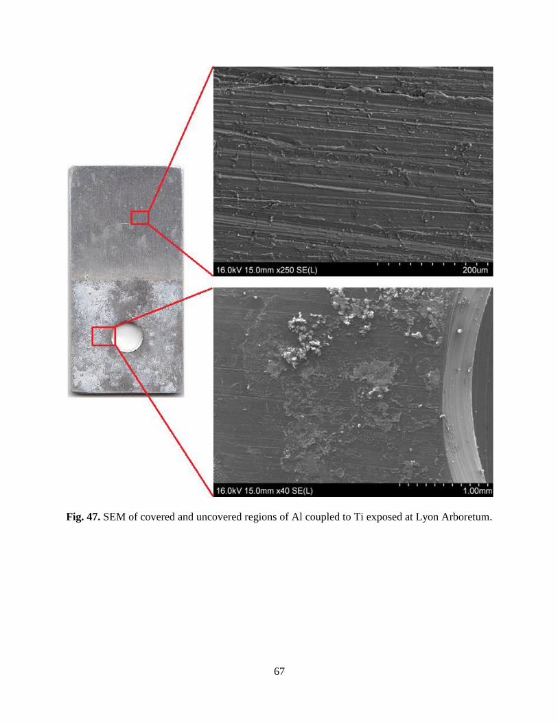
67

Fig. 47. SEM of covered and uncovered regions of Al coupled to Ti exposed at Lyon Arboretum.

68

Fig. 48. SEM of covered and uncovered regions of Al coupled to stainless steel exposed at

Lyon Arboretum.

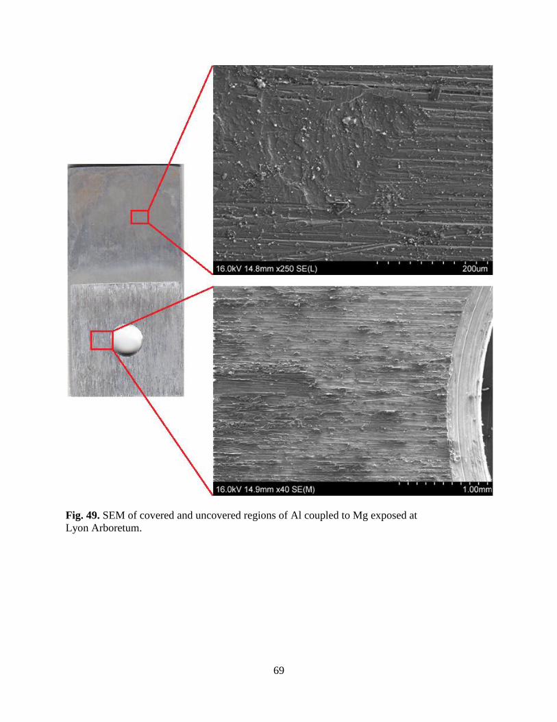
69

Fig. 49. SEM of covered and uncovered regions of Al coupled to Mg exposed at

Lyon Arboretum.

70

6.1.3. Test specimens at Kilauea Volcanoes National Park

Surface analysis of the uncoupled Al exposed at Kilauea yielded unique results. While

the corrosion rate was found to be comparable to the other outdoor test sites, the high atomic

percentage of sulfur found in the pits on the surface of the uncoupled Al were exclusive to this

test site (Table 35). In a volcanic environment, sulfur originates from of sulfur dioxide which

reacts with oxygen and water in the environment to form sulfuric acid. The sulfur detected using

EDXA is likely in the form of a sulfate salt.

Fig. 50. SEM of uncoupled Al exposed at Kilauea.


Element Al O C Mg Si S Fe Cr Na

Atomic %

Region 78.9 15.0 4.17 0.76 0.5 0.32 0.22 0.12 0.29

Pit 70.2 18.9 0.34 0.33 2.99 6.30 0.71

Elemental analysis of corroded regions of Al coupled to Ag as well as the Al coupled to

Cu showed contamination of the uncovered region by their respective coupled metals (Tables 36

and 37). Further analysis into a pit on the Al coupon coupled to Cu showed an increased amount

of copper present in the pit. This suggests that the pitting was initiated or propagated by copper

migration from the Cu coupon to the uncovered region of the Al coupon.

71

Fig. 51. SEM of uncovered region of Al coupled to Ag exposed at Kilauea.


Element O Al S C Si Ag

Atomic % 73.6 18.6 4.25 2.85 0.50 0.14

Fig. 52. SEM of uncovered region of Al coupled to Cu exposed at Kilauea.

72


Element O Al S C Mg Si Cu Fe

Atomic % Region 62.3 31.5 2.95 2.80 0.27 0.20 <0.00

Pit 45.1 48.4 3.71 0.65 1.81 0.32

The sets of Al coupled to either Ti or stainless steel had a roughly equal corrosion rate.

The morphology of the surfaces of these Al coupons were similar (Figs. 53 and 54), as are their

elemental compositions (Tables 38 and 39).

Fig. 53. SEM of uncovered region of Al coupled to Ti exposed at Kilauea.


Element O Al C S Si Mg Na Cl Fe

Atomic % 54.7 35.6 5.95 2.5 0.47 0.29 0.19 0.26 0.11

73

Fig. 54. SEM of uncovered region of Al coupled to stainless steel exposed at Kilauea.


Element O Al S C Si Na Fe

Atomic % 70.3 22.2 3.62 3.24 0.39 0.20 0.12

On the uncovered surface of the Al coupled to stainless steel, a pit was magnified in order

to obtain a pointwise elemental analysis of this corroded region (Fig. 55). At a magnification of

4000x an inclusion was found containing a high amount of silicon, a major alloying element.

Other alloying elements were included in the elemental analysis such as iron and titanium. The

composition inside this pit is shown in Table 40.

74

Fig. 55. SEM of pit on the uncovered region of Al coupled to stainless steel at Kilauea.

Table 40: Elemental composition of inclusion shown in Fig. 55.

Element O Si Al Ca Mg Fe Na Ti K S

Atomic % 67 14.8 8.16 2.87 2.87 2.33 1.1 0.52 0.27 0.16

A micrograph of Al coupled to mild steel was taken at the longitudinal edge of the

uncovered surface (Fig. 56). The elemental analysis shows a high percentage of iron even at the

furthest point from the actual mild steel coupon (Table 41). The migration of the corrosion

product from the mild steel may have contributed to the relatively high corrosion rate compared

to the Al coupled to the passivating metals.

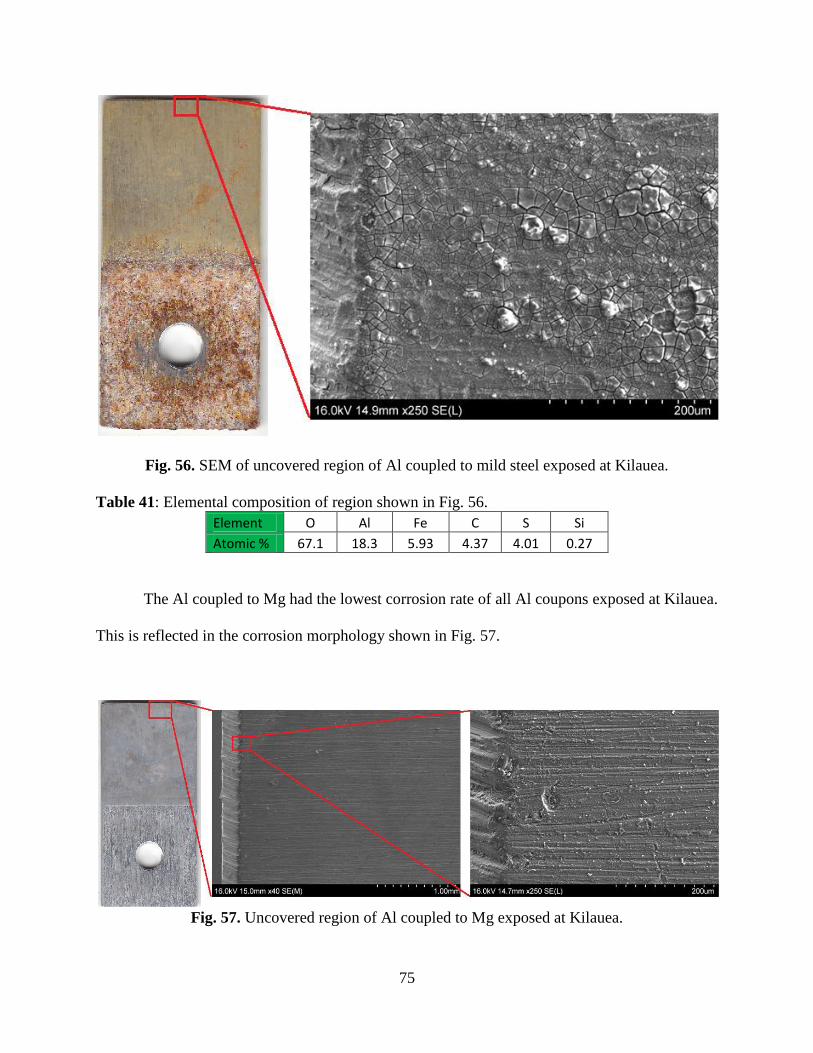
75

Fig. 56. SEM of uncovered region of Al coupled to mild steel exposed at Kilauea.


Element O Al Fe C S Si

Atomic % 67.1 18.3 5.93 4.37 4.01 0.27

The Al coupled to Mg had the lowest corrosion rate of all Al coupons exposed at Kilauea.

This is reflected in the corrosion morphology shown in Fig. 57.

Fig. 57. Uncovered region of Al coupled to Mg exposed at Kilauea.

76

6.1.4. Test specimens in the cyclic corrosion testing chamber

Corrosion morphology in the Al coupons exposed in the CCTC was difficult to view in

the uncoupled Al coupons as well as in the uncovered regions of the coupled Al coupons. This

was due to the thick layer of salt deposited on the exposed surface of the Al from the accelerated

corrosion test. A typical exposed region is shown in Fig. 58 which shows an Al coupon that was

coupled to stainless steel following 30 cycles of the GM-9540P test; this region was subjected to

elemental analysis. The region was further magnified and elemental analysis was again taken,

showing an elemental composition predominated by calcium carbonate. Compositions of these

regions are shown in Table 42.

Fig. 58. SEM of uncovered region of Al coupled to stainless steel exposed in the CCTC.


Element O Al C Ca Na Fe Cl

Atomic % Region 1 74.6 20.6 3.63 0.74 0.23 0.15 0.12

Region 2 68.9 3.14 15.8 12.2

In the covered region, however, some regions of the Al were exposed. In one such region

on the Al coupon coupled to Ag, an abundance of unfamiliar flakes of product were found

77

(Fig. 59). The elemental analysis on these products showed a composition of mostly silver and

oxygen and are thought to be elemental silver or silver oxide from the Ag coupon (Table 43).

Fig. 59. SEM of covered region of Al coupled to Ag exposed in the CCTC.


Element O Al C Na Ag Ca Mg

Atomic % Region 74.9 16.9 3.8 2.21 1.21 0.71 0.24

Flakes 50.7 2.85 1.00 42.8 0.39

Both covered and uncovered regions of Al coupled to Cu were obscured by thick layers

of product and the base Al underneath was difficult to view using SEM. Fig. 60 is a micrograph

of the product covering the Al coupon in the region of the couple underneath the Cu coupon; the

corresponding elemental analysis of this layer is shown in Table 44.

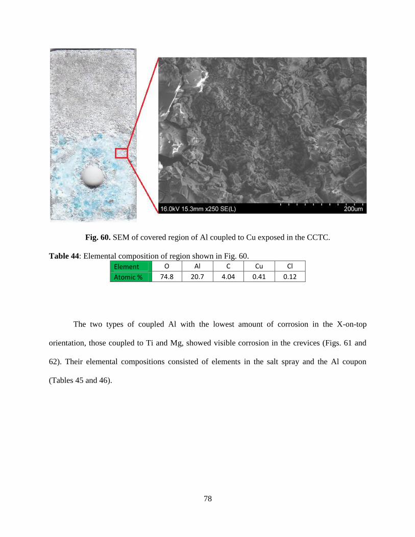
78

Fig. 60. SEM of covered region of Al coupled to Cu exposed in the CCTC.


Element O Al C Cu Cl

Atomic % 74.8 20.7 4.04 0.41 0.12

The two types of coupled Al with the lowest amount of corrosion in the X-on-top

orientation, those coupled to Ti and Mg, showed visible corrosion in the crevices (Figs. 61 and

62). Their elemental compositions consisted of elements in the salt spray and the Al coupon

(Tables 45 and 46).

79

Fig. 61. SEM of uncovered region of Al coupled to Ti exposed in the CCTC.


Element O Al C Na Ca Cl Ti

Atomic % 75.3 21.8 2.36 0.33 0.12 0.11 <0.00

Fig. 62. SEM of uncovered region of Al coupled to Mg exposed in the CCTC.

80


Element O Al Mg C Na Ca

Atomic % 75.3 16.8 4.22 3.30 0.28 0.10

The covered region of the Al coupled to Fe was similar to that of the Al coupled to Cu in

that the layer of corrosion product from the coupling metal was abundant and did not uncover the

Al surface underneath (Fig. 63). The composition of this corrosion product layer is shown in

Table 47. The layer is shown to consist of mostly iron and aluminum oxides, as well as elements

from the salt spray.

Fig. 63. SEM of covered region of Al coupled to mild steel exposed in the CCTC.


Element O Al Fe C Na

Atomic % 67.5 16.6 11.5 2.92 1.51

81

6.2. X-ray diffraction analysis

X-ray diffraction (XRD) analysis was performed using a Rigaku MiniFlex II Desktop X-

ray Diffractometer on the corroded Al samples from the sets of uncoupled Al and coupled Al in

the X-on-top orientation. Diffraction patterns for the coupled Al were obtained in the region

covered by the corresponding metal in order to obtain a comparison of corrosion product.

Comparisons were performed between a single type of Al set at every exposure location as well

as between every type of Al set at a single exposure location. The International Centre for

Diffraction Data library was used to characterize peaks displayed in the spectra.

6.2.1. Comparison of Al spectra by location

In order to identify corrosion products formed by exposure, an initial spectra of virgin

unexposed Al was obtained (Fig. 64). In descending order of intensity, the peaks identified were

of 44.7°, 38.4°, 65.1°, 78.2°, 82.4°, and 22.4°. These peaks were used to identify which peaks in

the spectra of the exposed Al were of the base metal itself.

Fig. 64. XRD spectra of virgin Al coupon.

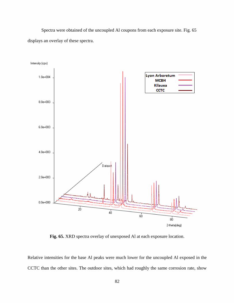
82

Spectra were obtained of the uncoupled Al coupons from each exposure site. Fig. 65

displays an overlay of these spectra.

Fig. 65. XRD spectra overlay of unexposed Al at each exposure location.

Relative intensities for the base Al peaks were much lower for the uncoupled Al exposed in the

CCTC than the other sites. The outdoor sites, which had roughly the same corrosion rate, show

83

similar intensities in their base metal peaks. The two peaks shown at 18.8° and 20.3° correspond

to the peaks of aluminum hydroxide Al(OH)3, a common corrosion product of aluminum when

reacted with water. Additional peaks in the unexposed Al from the CCTC at 23.1°, 29.4°, 31.4°,

39.4°, 43.1°, 47.5°, and 48.5° correspond to calcium carbonate CaCO3 which during SEM and

EDXA analysis was shown to be abundant on the samples exposed in the CCTC. The Al exposed

at MCBH also display low peaks in the ranges of calcium carbonate.

The spectra of Al coupled to Ag are displayed in Fig. 66. The Al(OH)3 peaks appeared

for all test sites except for Kilauea at which Al had the lowest corrosion rate. The intensity of the

base metal peaks for the Al at Kilauea also remained much higher than the Al exposed at the

other test sites. The higher intensity of the base metal peaks also indicated that the oxide film

was thinner, which could also be attributed to the acid rain at Kilauea that dissolved the

aluminum oxide corrosion products preventing its buildup. Calcium carbonate on the sample

from the CCTC remained abundant.

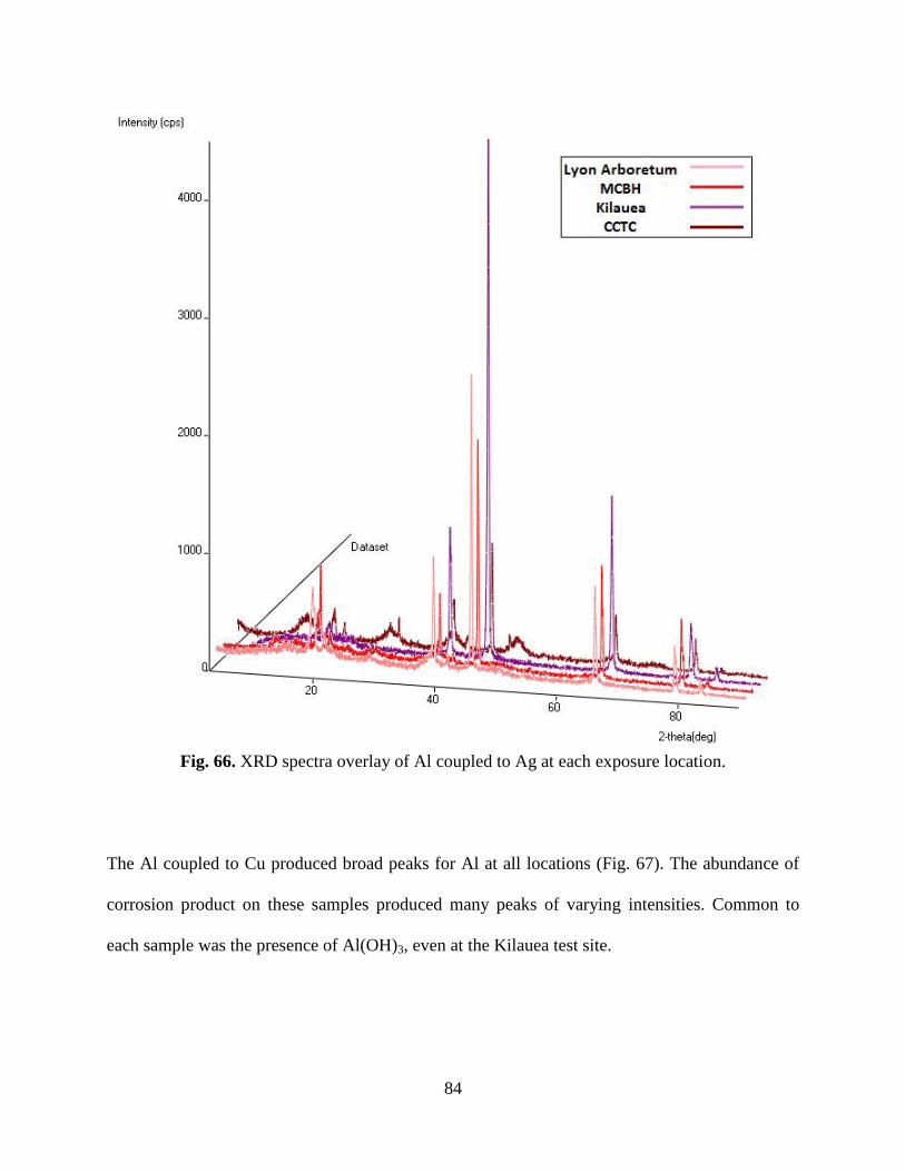
84

Fig. 66. XRD spectra overlay of Al coupled to Ag at each exposure location.

The Al coupled to Cu produced broad peaks for Al at all locations (Fig. 67). The abundance of

corrosion product on these samples produced many peaks of varying intensities. Common to

each sample was the presence of Al(OH)3, even at the Kilauea test site.

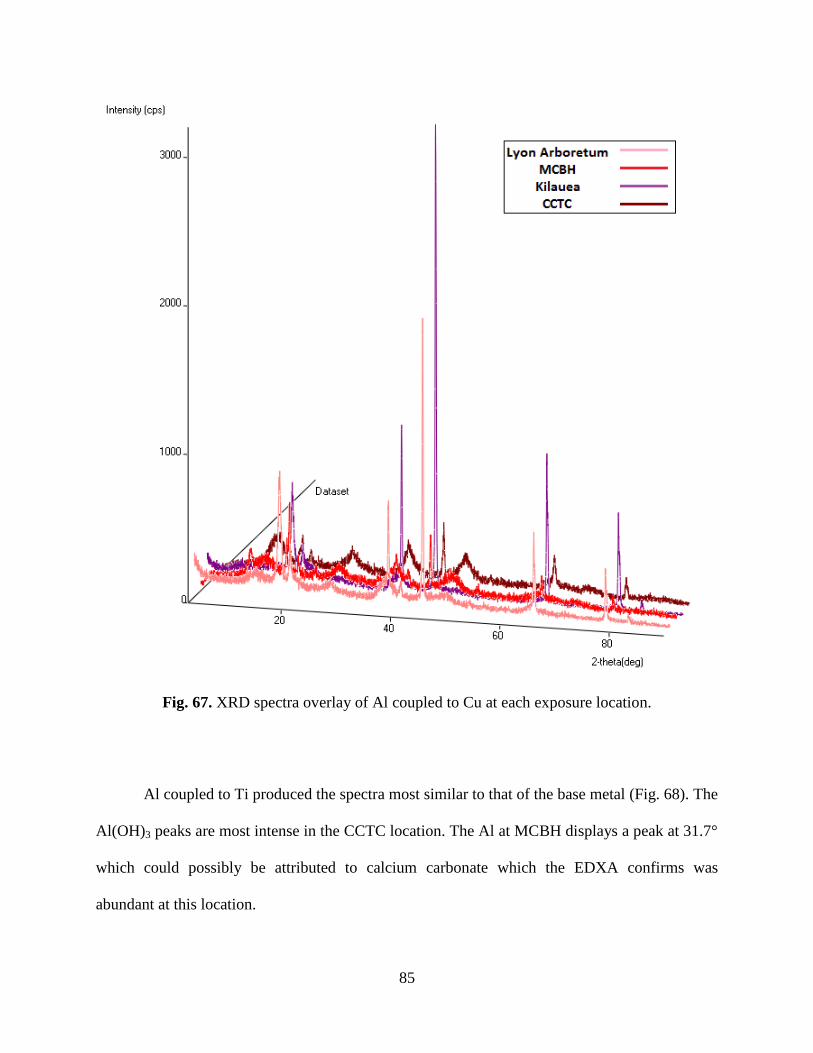
85

Fig. 67. XRD spectra overlay of Al coupled to Cu at each exposure location.

Al coupled to Ti produced the spectra most similar to that of the base metal (Fig. 68). The

Al(OH)3 peaks are most intense in the CCTC location. The Al at MCBH displays a peak at 31.7°

which could possibly be attributed to calcium carbonate which the EDXA confirms was

abundant at this location.

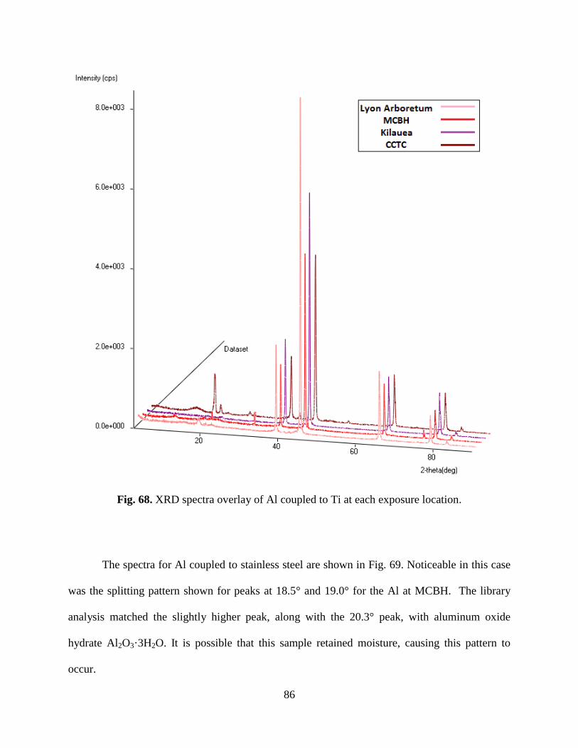
86

Fig. 68. XRD spectra overlay of Al coupled to Ti at each exposure location.

The spectra for Al coupled to stainless steel are shown in Fig. 69. Noticeable in this case

was the splitting pattern shown for peaks at 18.5° and 19.0° for the Al at MCBH. The library

analysis matched the slightly higher peak, along with the 20.3° peak, with aluminum oxide

hydrate Al2O3·3H2O. It is possible that this sample retained moisture, causing this pattern to

occur.

87

Fig. 69. XRD spectra overlay of Al coupled to stainless steel at each exposure location.

Similar to the Al coupled to Cu, the Al coupled to mild steel produced spectra with very

broad peaks and low intensity due to the thick layer of corrosion product present on the sample

(Fig. 70). Albeit with the lowest intensity compared to every other Al couple type, Al(OH)3

peaks were identified at the Lyon Arboretum, MCBH, and Kilauea sites. These peaks were not

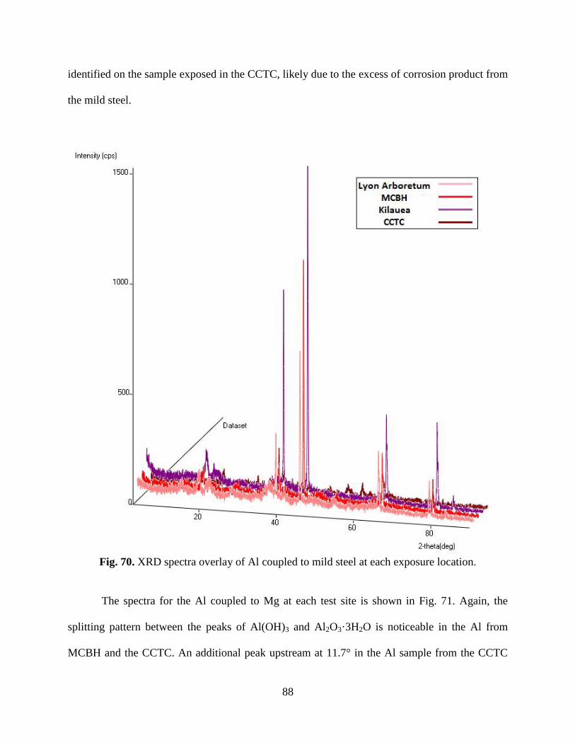
88

identified on the sample exposed in the CCTC, likely due to the excess of corrosion product from

the mild steel.

Fig. 70. XRD spectra overlay of Al coupled to mild steel at each exposure location.

The spectra for the Al coupled to Mg at each test site is shown in Fig. 71. Again, the

splitting pattern between the peaks of Al(OH)3 and Al2O3·3H2O is noticeable in the Al from

MCBH and the CCTC. An additional peak upstream at 11.7° in the Al sample from the CCTC

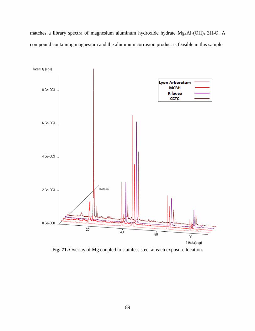
89

matches a library spectra of magnesium aluminum hydroxide hydrate Mg4Al2(OH)4·3H2O. A

compound containing magnesium and the aluminum corrosion product is feasible in this sample.

Fig. 71. Overlay of Mg coupled to stainless steel at each exposure location.

90

6.2.2. Comparison of Al spectra by couple type

The comparison of each spectra by the metal to which it was coupled shows the

intensities of the peaks relative to each other in order to highlight the differences in corrosion

behavior. Spectra of each type of Al sample exposed at Lyon Arboretum are shown in Fig. 72.

Fig. 72. XRD spectra overlay of all exposed Al types at Lyon Arboretum.

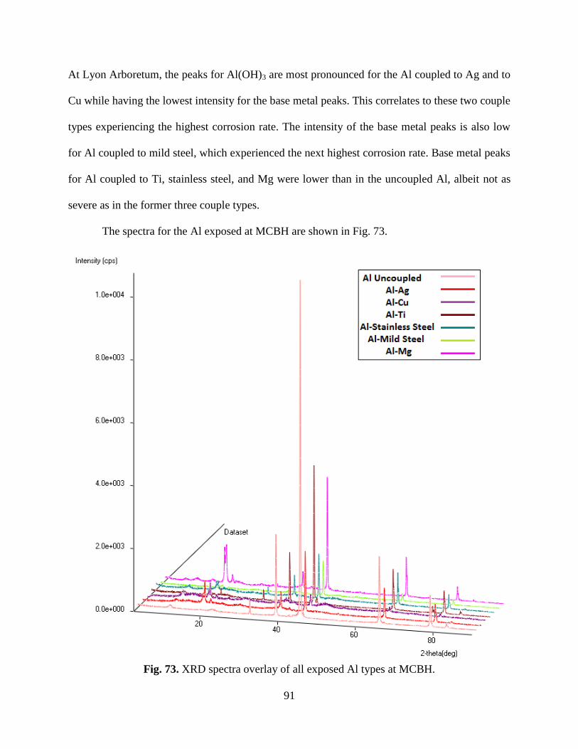
91

At Lyon Arboretum, the peaks for Al(OH)3 are most pronounced for the Al coupled to Ag and to

Cu while having the lowest intensity for the base metal peaks. This correlates to these two couple

types experiencing the highest corrosion rate. The intensity of the base metal peaks is also low

for Al coupled to mild steel, which experienced the next highest corrosion rate. Base metal peaks

for Al coupled to Ti, stainless steel, and Mg were lower than in the uncoupled Al, albeit not as

severe as in the former three couple types.

The spectra for the Al exposed at MCBH are shown in Fig. 73.

Fig. 73. XRD spectra overlay of all exposed Al types at MCBH.

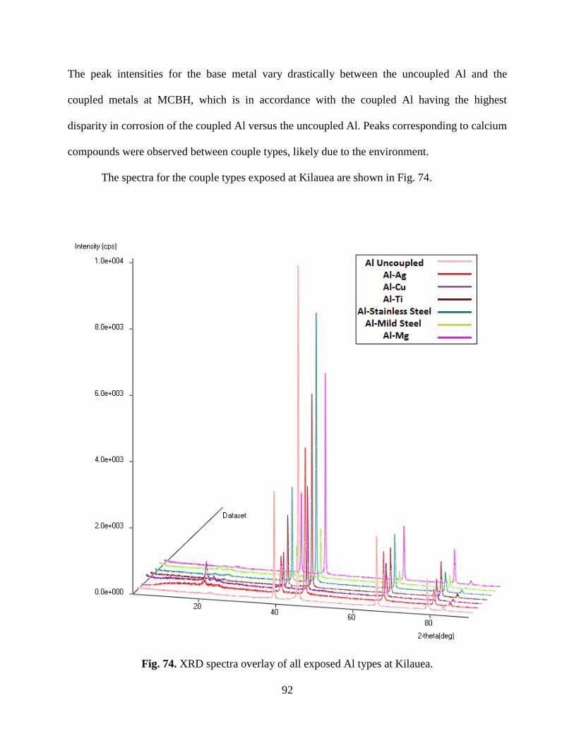
92

The peak intensities for the base metal vary drastically between the uncoupled Al and the

coupled metals at MCBH, which is in accordance with the coupled Al having the highest

disparity in corrosion of the coupled Al versus the uncoupled Al. Peaks corresponding to calcium

compounds were observed between couple types, likely due to the environment.

The spectra for the couple types exposed at Kilauea are shown in Fig. 74.

Fig. 74. XRD spectra overlay of all exposed Al types at Kilauea.

93

Similar to Lyon Arboretum, the presence of Al(OH)3 is most noticeable for the Al coupled to Ag

and Cu with slight peaks seen for Al coupled to mild steel. Although the Al coupled to Ti and

stainless steel experienced roughly the same corrosion rate, the peak intensities for Al-Ti are

generally lower than those for Al-stainless steel. This may be due to the region in which the

spectra was obtained; the covered region of Al may have been more corroded in the Al-Ti couple

than for the Al-stainless steel couple.

Fig. 75 displays the spectra for all exposed Al types in the CCTC. Here we see an

extremely high intensity peak for Al which was coupled to Mg—this is likely due to the

combination of both aluminum hydroxide and magnesium hydroxide. Al(OH)3 peaks are seen for

most samples including the uncoupled Al, though by comparison the intensity of these peaks for

Al coupled to mild steel is relatively low. However, since Al coupled to mild steel had the third

highest corrosion rate in the CCTC, this again may be attributed to the large amount of corrosion

product obscuring the diffraction of the Al.

94

Fig. 75. Overlay of all exposed Al types in the CCTC.

95

Chapter 7: Conclusions

The results of the potentiodynamic polarization experiments highlight the

importance of field data in conjunction with laboratory data. While the mild steel acted was

anodic to Al in the sodium sulfate solution, in every iteration of exposure testing the galvanic

current data showed that mild steel was the cathode when coupled to Al. Also of significance

regarding outdoor testing is that even when exposed in a naturally chloride-heavy marine

environment, the uncoupled Al retained its passive layer and was highly resistant to corrosion;

whereas, in the accelerated test chamber, the combination of cyclic salt spraying, high humidity,

and high temperatures up to 60°C significantly caused more passive-film breakdown and pitting,

lowering the ratio of total corrosion between the coupled Al versus the uncoupled Al. The

Kilauea test site was expected to have the third highest corrosion rate due to the proximity of the

ocean to the volcano; however, in practice Lyon Arboretum proved to be the more corrosive

environment.

For all couple types in which Al was the anode, galvanic current only accounted for a

small fraction of the total mass loss. Local corrosion was likely accelerated due to the

development of pH gradients caused by the separation of the anode and cathode. The physical

coupling of Al to another metal also increases corrosion due to crevice corrosion in addition to

galvanic coupling. For the noble metals, the composition analysis of the pits in the region of Al

not covered by the Cu or Ag coupons showed an increased amount of these elements; this

suggests local corrosion acceleration by precipitation of Cu or Ag onto the Al surface creating

cathodic sites. For the mild steel, iron corrosion products were abundantly present on the Al

surface both in the uncovered and covered regions, which may have also accelerated corrosion.

For the passivating alloys, i.e. stainless steel and Ti, the contamination of the Al by these metals

96

was minimal, suggesting that the corrosion-accelerating factors in addition to galvanic corrosion

were pH gradients and crevice corrosion. Thus, in practice, the total corrosion of many types of

an aluminum-containing galvanic couple may not be estimated simply by the galvanic

component of corrosion in addition to the local corrosion rate as calculated by uncoupled

aluminum.

The Mg did not show as dramatic a difference in the local corrosion of the uncoupled

metal versus the coupled Mg. The fraction of calculated galvanic corrosion to actual total

corrosion of Al was fairly consistent with the component of local corrosion as calculated by the

mass loss of the uncoupled Mg. Without the ability to passivate and also being an active metal,

Mg does not have the innate corrosion resistance as Al does and, thus, does not exhibit radically

different corrosion behavior in a galvanic couple apart from local corrosion in conjunction with

galvanic corrosion.

Consistent with the literature, the chloride-heavy environments, i.e. MCBH and the GM-

9540P test in the CCTC, caused the highest amount of corrosion. The XRD data shows that the

Al at these two sites produce the main Al corrosion product Al(OH)3 the most consistently across

all couple types. Although less corrosive than the high chloride-containing sites, the volcanic site

has acid rain due to the emission of SO2. Accordingly, high concentrations of sulfur (likely in

the form of sulfate) were found in the pits on Al. The anionic SO42-

is likely to migrate into the

anodic pit. The average calculated mass loss due to galvanic current was higher for all couple

types at Lyon Arboretum versus Kilauea. This increase in galvanic current is thought to be due to

the extremely humid and rainy environment at Lyon Arboretum; wherein, the couples are

consistently exposed to the electrolyte creating a salt bridge and therefore galvanic current.

97

References 1Wesley, W. A.; Brown, R. H. In The Corrosion Handbook; Uhlig, H. H., Ed.; John Wiley &

Sons: New York, 1948; pp 481–496.

2Revie, R. W.; Uhlig, H. H. Corrosion and Corrosion Control: An Introduction to Corrosion

Science and Engineering, 4th ed.; John Wiley & Sons: Hoboken, NJ, 2008.

3Huang, I.-W.; Hurley, B. L.; Yang, F.; Buchheit, R. G. Electrochim. Acta 2016, 199, 242–253.

4Mccafferty, E. Corros. Sci. 2003, 45 (7), 1421–1438.

5Szklarska-Smialowska, Z. Corros. Sci. 1999, 41 (9), 1743–1767.

6Blanc, C.; Mankowski, G. Corros. Sci. 1997, 39 (5), 949–959.

7Datta, J.; Bhattacharya, C.; Bandyopadhyay, S. B. Mater. Sci. 2005, 28 (3), 253–258.

8Dan, Z.; Muto, I.; Hara, N. Corros. Sci. 2012, 57, 22–29.

9Cui, Z. Y.; Li, X. G.; Man, C.; Xiao, K.; Dong, C. F.; Wang, X.; Liu, Z. Y. J. Mater. Eng.

Perform. 2015, 24 (8), 2885–2897.

10

Ezuber, H.; El-Houd, A.; El-Shawesh, F. Mater. Design 2008, 29 (4), 801–805.

11

Acevedo-Hurtado, P. O.; Sundaram, P. A.; Caceres-Valencia, P. G.; Fachini, E. R.; Miller,

C.E.; Placzankis, B. E. Corros. Sci. 2008, 50 (11), 3123–3131.

12

Raj, X. J.; Nishimura, T. Prot. Met. Phys. Chem. Surf. 2016, 52 (3), 543–554.

13

Rafla, V.; King, A. D.; Glanvill, S.; Parsons, A.; Davenport, A.; Scully, J. R. Corrosion 2015,

71 (10), 1171–1176.

14

Vera, R.; Verdugo, P.; Orellana, M.; Muñoz, E. Corros. Sci. 2010, 52 (11), 3803–3810.

15

Lacroix Lo c lanc, C. P b re Nadine; Tribollet, B.; Vivier, V. J.Electrochem. Soc. 2009, 156

(8).

16

Younan, H.; Zhiqiang, M.; Siping, Z.; Hao, G. In ISTFA 2007, Proceedings of the 33rd

International Symposium for Testing and Failure Analysis, San Jose, CA, Nov 4-8, 2007;

ASM International; pp 193-196.

17

Caspers, H. The Ocean: A Scientific American Book; WH Freeman & Co: San Francisco, CA,

1969.

18

Hatch, J.E. Aluminum: Properties and Physical Metallurgy; ASM International, 1984.

Documents

GALVANIC CORROSION OF ALUMINUM COUPLED TO … · The total corrosion on an anode in a galvanic couple results from galvanic corrosion between the anode and the cathode plus additional