Embed Size (px)
Citation preview
2009 CERN Summer Student Lectures on Statistics 1G. Cowan
Introduction to Statistics − Day 4Lecture 1
ProbabilityRandom variables, probability densities, etc.
Lecture 2Brief catalogue of probability densitiesThe Monte Carlo method.
Lecture 3Statistical testsFisher discriminants, neural networks, etc Significance and goodness-of-fit tests
Lecture 4Parameter estimationMaximum likelihood and least squaresInterval estimation (setting limits)
→
2009 CERN Summer Student Lectures on Statistics 2G. Cowan
Parameter estimationThe parameters of a pdf are constants that characterize its shape, e.g.
r.v.
Suppose we have a sample of observed values:
parameter
We want to find some function of the data to estimate the parameter(s):
← estimator written with a hat
Sometimes we say ‘estimator’ for the function of x1, ..., xn;‘estimate’ for the value of the estimator with a particular data set.
2009 CERN Summer Student Lectures on Statistics 3G. Cowan
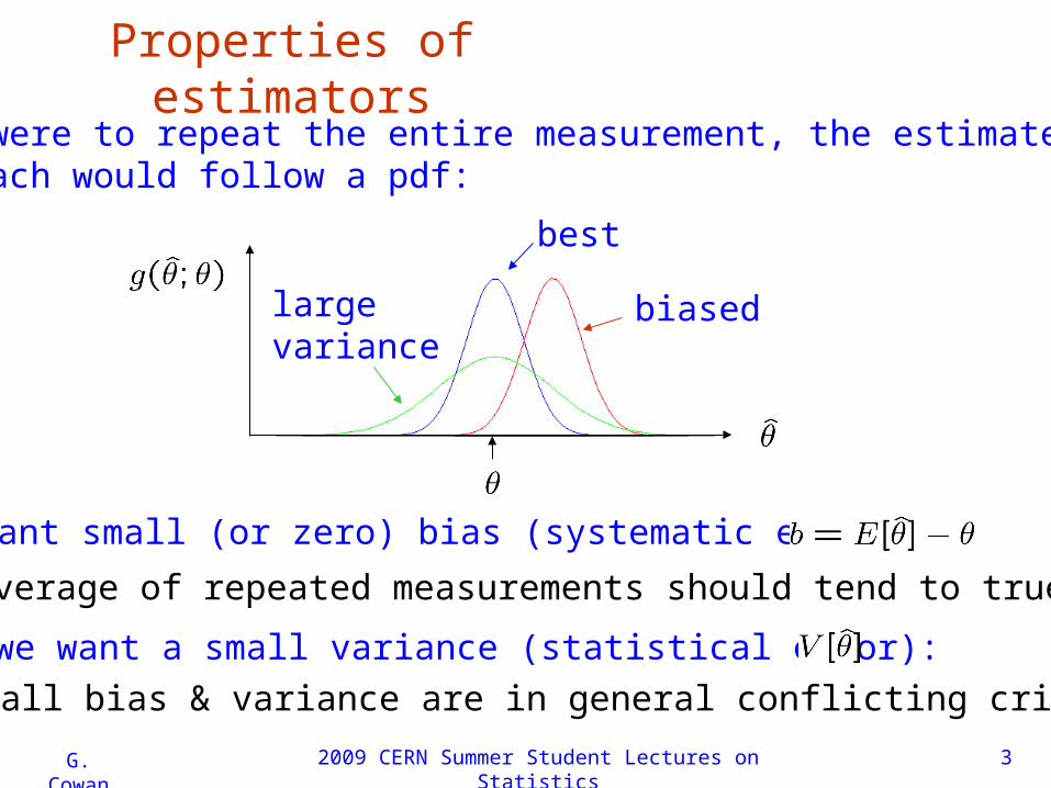
Properties of estimatorsIf we were to repeat the entire measurement, the estimatesfrom each would follow a pdf:
biasedlargevariance
best
We want small (or zero) bias (systematic error):
→ average of repeated measurements should tend to true value.
And we want a small variance (statistical error):
→ small bias & variance are in general conflicting criteria

2009 CERN Summer Student Lectures on Statistics 4G. Cowan
An estimator for the mean (expectation value)
Parameter:
Estimator:
We find:
(‘sample mean’)

2009 CERN Summer Student Lectures on Statistics 5G. Cowan
An estimator for the variance
Parameter:
Estimator:
(factor of n1 makes this so)
(‘samplevariance’)
We find:
where
2009 CERN Summer Student Lectures on Statistics 6G. Cowan
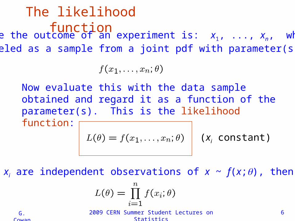
The likelihood functionSuppose the outcome of an experiment is: x1, ..., xn, whichis modeled as a sample from a joint pdf with parameter(s) :
Now evaluate this with the data sample obtained and regard it as a function of the parameter(s). This is the likelihood function:
(xi constant)
If the xi are independent observations of x ~ f(x;), then,
2009 CERN Summer Student Lectures on Statistics 7G. Cowan
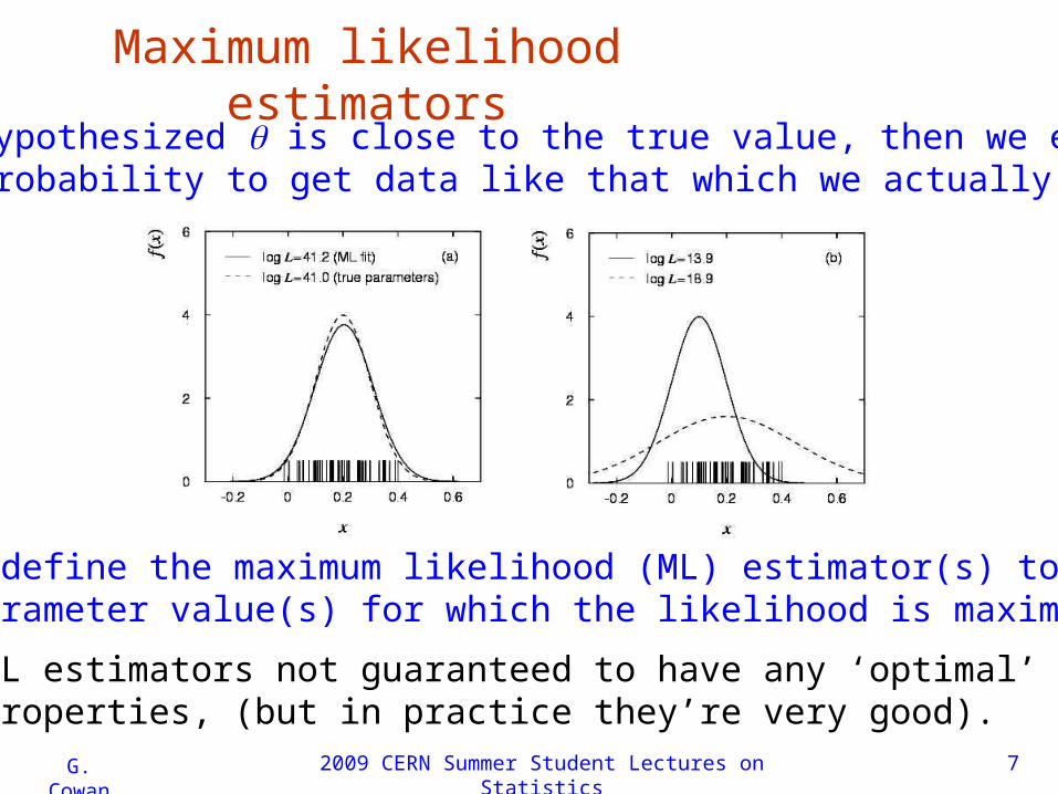
Maximum likelihood estimatorsIf the hypothesized is close to the true value, then we expect a high probability to get data like that which we actually found.
So we define the maximum likelihood (ML) estimator(s) to be the parameter value(s) for which the likelihood is maximum.
ML estimators not guaranteed to have any ‘optimal’properties, (but in practice they’re very good).
2009 CERN Summer Student Lectures on Statistics 8G. Cowan
ML example: parameter of exponential pdf
Consider exponential pdf,
and suppose we have data,
The likelihood function is
The value of for which L() is maximum also gives the maximum value of its logarithm (the log-likelihood function):

2009 CERN Summer Student Lectures on Statistics 9G. Cowan
ML example: parameter of exponential pdf (2)
Find its maximum by setting
→
Monte Carlo test: generate 50 valuesusing = 1:
We find the ML estimate:
2009 CERN Summer Student Lectures on Statistics 10G. Cowan
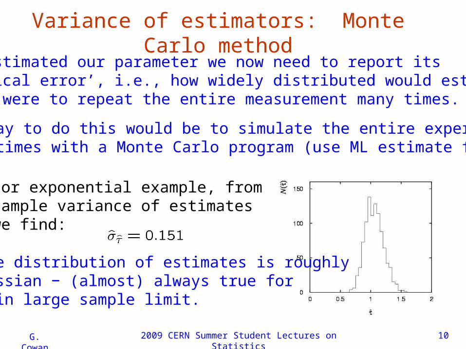
Variance of estimators: Monte Carlo methodHaving estimated our parameter we now need to report its‘statistical error’, i.e., how widely distributed would estimatesbe if we were to repeat the entire measurement many times.
One way to do this would be to simulate the entire experimentmany times with a Monte Carlo program (use ML estimate for MC).
For exponential example, from sample variance of estimateswe find:
Note distribution of estimates is roughlyGaussian − (almost) always true for ML in large sample limit.
2009 CERN Summer Student Lectures on Statistics 11G. Cowan
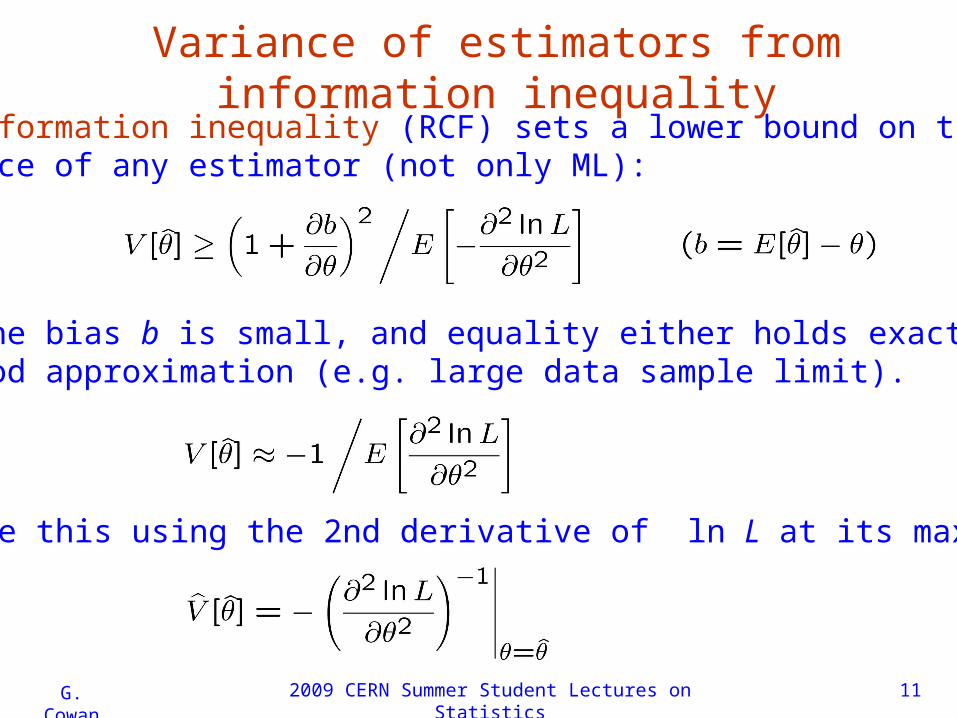
Variance of estimators from information inequalityThe information inequality (RCF) sets a lower bound on the variance of any estimator (not only ML):
Often the bias b is small, and equality either holds exactly oris a good approximation (e.g. large data sample limit). Then,
Estimate this using the 2nd derivative of ln L at its maximum:
2009 CERN Summer Student Lectures on Statistics 12G. Cowan
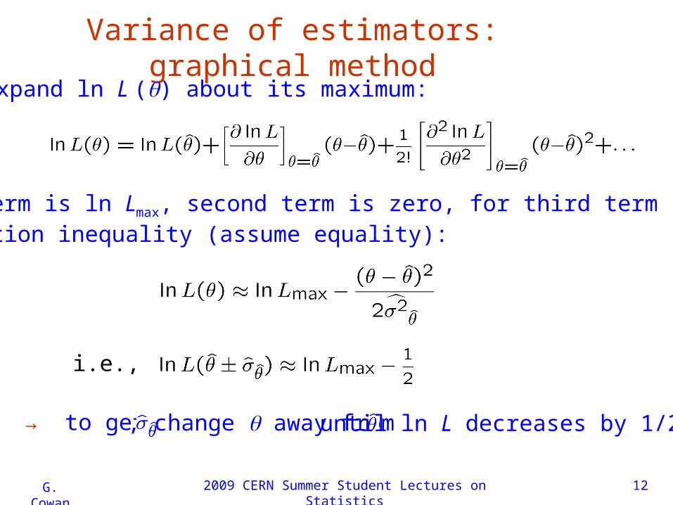
Variance of estimators: graphical methodExpand ln L () about its maximum:
First term is ln Lmax, second term is zero, for third term use information inequality (assume equality):
i.e.,
→ to get , change away from until ln L decreases by 1/2.
2009 CERN Summer Student Lectures on Statistics 13G. Cowan
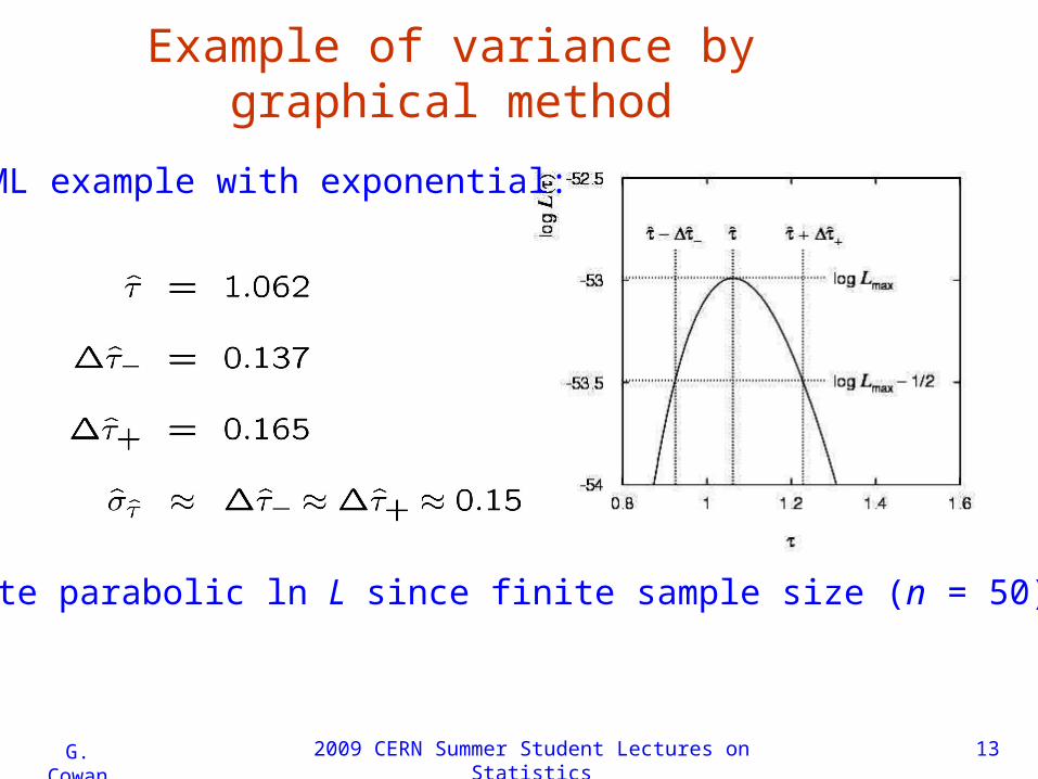
Example of variance by graphical method
ML example with exponential:
Not quite parabolic ln L since finite sample size (n = 50).

2009 CERN Summer Student Lectures on Statistics 14G. Cowan
The method of least squaresSuppose we measure N values, y1, ..., yN, assumed to be independent Gaussian r.v.s with
Assume known values of the controlvariable x1, ..., xN and known variances
The likelihood function is
We want to estimate , i.e., fit the curve to the data points.
2009 CERN Summer Student Lectures on Statistics 15G. Cowan
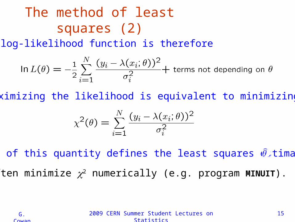
The method of least squares (2)
The log-likelihood function is therefore
So maximizing the likelihood is equivalent to minimizing
Minimum of this quantity defines the least squares estimator
Often minimize 2 numerically (e.g. program MINUIT).
2009 CERN Summer Student Lectures on Statistics 16G. Cowan
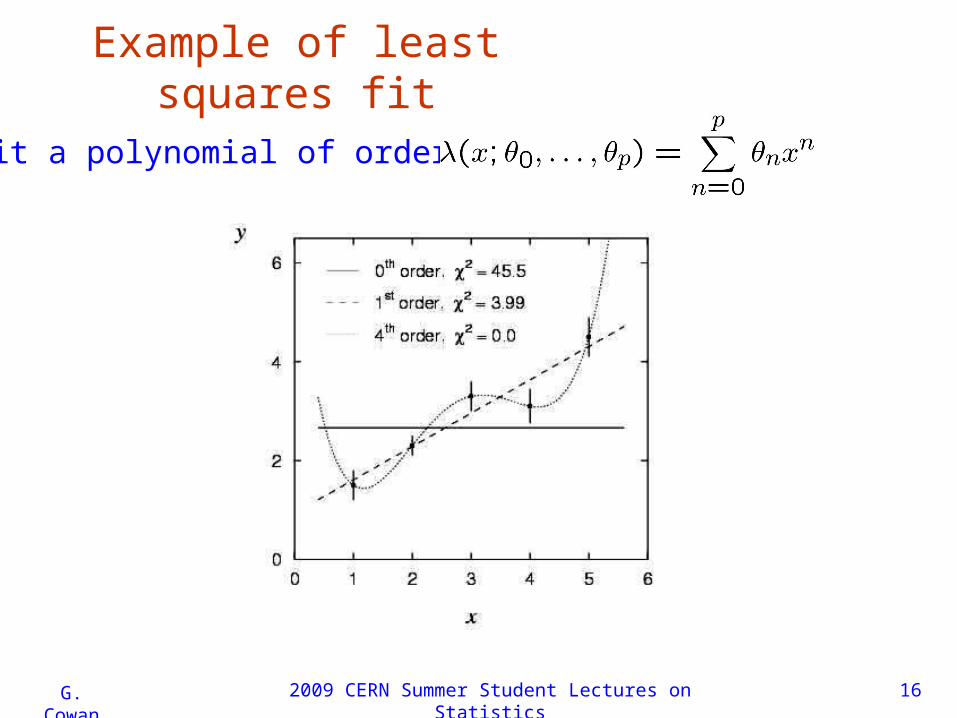
Example of least squares fit
Fit a polynomial of order p:
2009 CERN Summer Student Lectures on Statistics 17G. Cowan
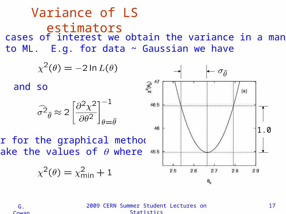
Variance of LS estimatorsIn most cases of interest we obtain the variance in a mannersimilar to ML. E.g. for data ~ Gaussian we have
and so
or for the graphical method we take the values of where
1.0
2009 CERN Summer Student Lectures on Statistics 18G. Cowan
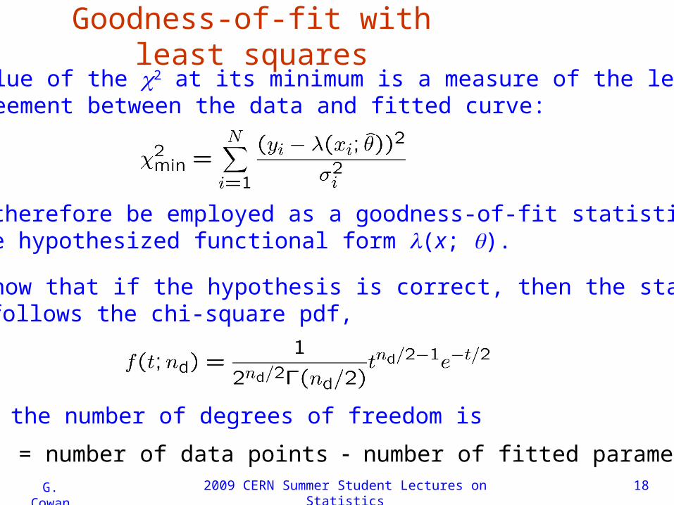
Goodness-of-fit with least squaresThe value of the 2 at its minimum is a measure of the levelof agreement between the data and fitted curve:
It can therefore be employed as a goodness-of-fit statistic totest the hypothesized functional form (x; ).
We can show that if the hypothesis is correct, then the statistic t = 2
min follows the chi-square pdf,
where the number of degrees of freedom is
nd = number of data points number of fitted parameters

2009 CERN Summer Student Lectures on Statistics 19G. Cowan
Goodness-of-fit with least squares (2)
The chi-square pdf has an expectation value equal to the number of degrees of freedom, so if 2
min ≈ nd the fit is ‘good’.
More generally, find the p-value:
E.g. for the previous example with 1st order polynomial (line),
whereas for the 0th order polynomial (horizontal line),
This is the probability of obtaining a 2min as high as the one
we got, or higher, if the hypothesis is correct.
2009 CERN Summer Student Lectures on Statistics 20G. Cowan
Setting limits
Consider again the case of finding n = ns + nb events where
nb events from known processes (background)ns events from a new process (signal)
are Poisson r.v.s with means s, b, and thus n = ns + nb
is also Poisson with mean = s + b. Assume b is known.
Suppose we are searching for evidence of the signal process,but the number of events found is roughly equal to theexpected number of background events, e.g., b = 4.6 and we observe nobs = 5 events.
→ set upper limit on the parameter s.
The evidence for the presence of signal events is notstatistically significant,
2009 CERN Summer Student Lectures on Statistics 21G. Cowan
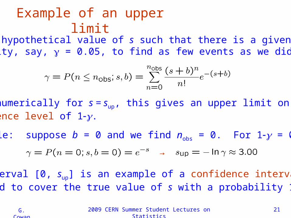
Example of an upper limit
Find the hypothetical value of s such that there is a given smallprobability, say, = 0.05, to find as few events as we did or less:
Solve numerically for s = sup, this gives an upper limit on s at aconfidence level of 1.
Example: suppose b = 0 and we find nobs = 0. For 1 = 0.95,
→
The interval [0, sup] is an example of a confidence interval,designed to cover the true value of s with a probability 1 .
2009 CERN Summer Student Lectures on Statistics 22G. Cowan
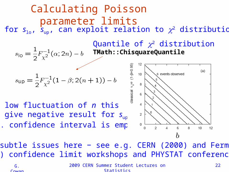
Calculating Poisson parameter limitsTo solve for slo, sup, can exploit relation to 2 distribution:
Quantile of 2 distributionTMath::ChisquareQuantile
For low fluctuation of n this can give negative result for sup; i.e. confidence interval is empty.
Many subtle issues here − see e.g. CERN (2000) and Fermilab(2001) confidence limit workshops and PHYSTAT conferences.
2009 CERN Summer Student Lectures on Statistics 23G. Cowan
Wrapping up lecture 4
We’ve seen some main ideas about parameter estimation,
ML and LS,how to obtain/interpret stat. errors from a fit,
and what to do if you don’t find the effect you’re looking for,
setting limits.
In four days we’ve only looked at some basic ideas and tools,skipping entirely many important topics. Keep an eye out fornew methods, especially multivariate, machine learning, Bayesian methods, etc.
2009 CERN Summer Student Lectures on Statistics 24G. Cowan
Extra slides
2009 CERN Summer Student Lectures on Statistics 25G. Cowan
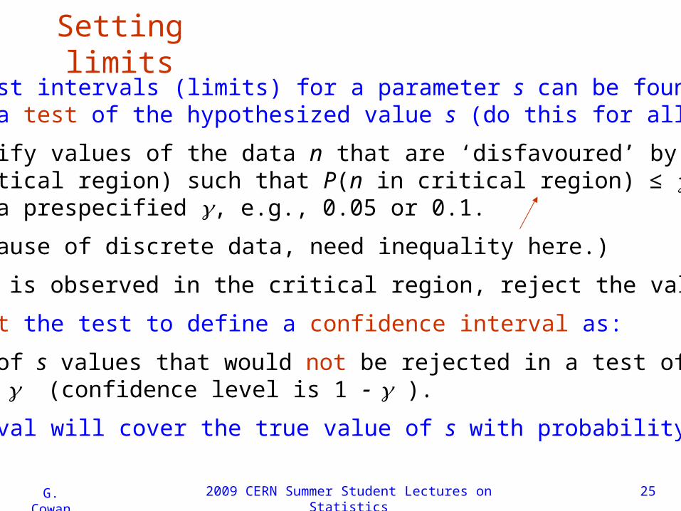
Setting limitsFrequentist intervals (limits) for a parameter s can be found by defining a test of the hypothesized value s (do this for all s):
Specify values of the data n that are ‘disfavoured’ by s (critical region) such that P(n in critical region) ≤ for a prespecified , e.g., 0.05 or 0.1.
(Because of discrete data, need inequality here.)
If n is observed in the critical region, reject the value s.
Now invert the test to define a confidence interval as:
set of s values that would not be rejected in a test ofsize (confidence level is 1 ).
The interval will cover the true value of s with probability ≥ 1 .
2009 CERN Summer Student Lectures on Statistics 26G. Cowan
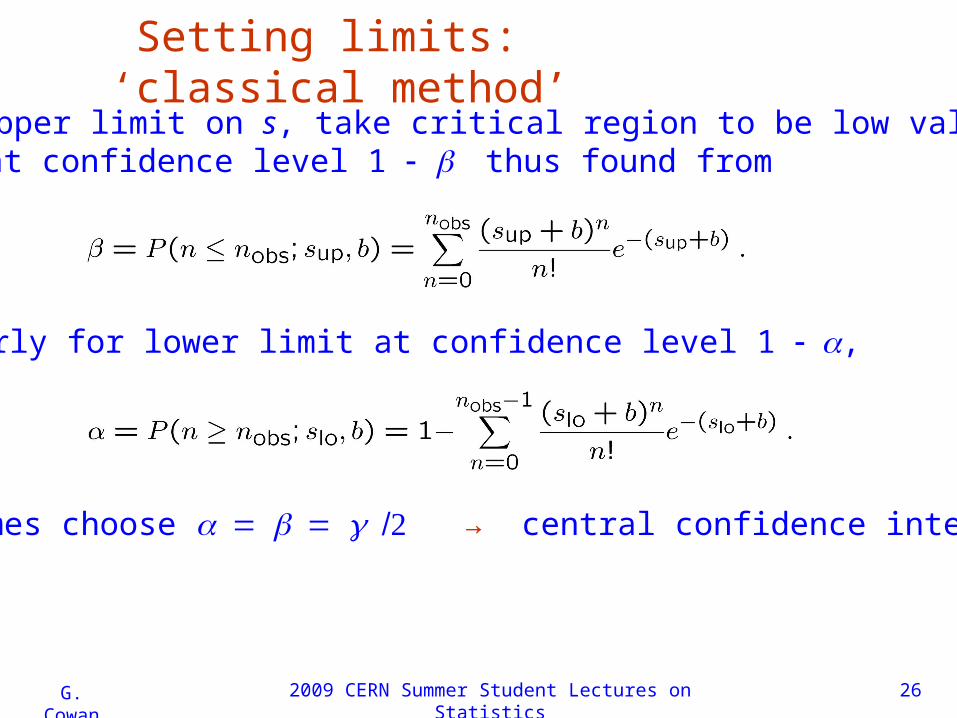
Setting limits: ‘classical method’E.g. for upper limit on s, take critical region to be low values of n, limit sup at confidence level 1 thus found from
Similarly for lower limit at confidence level 1 ,
Sometimes choose → central confidence interval.
2009 CERN Summer Student Lectures on Statistics 27G. Cowan
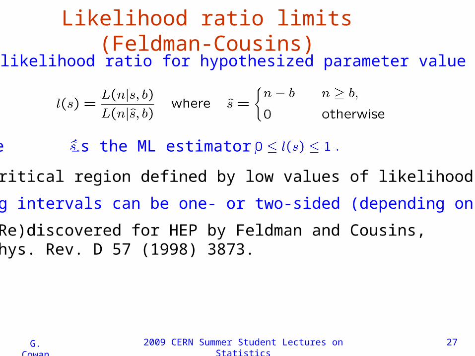
Likelihood ratio limits (Feldman-Cousins)Define likelihood ratio for hypothesized parameter value s:
Here is the ML estimator, note
Critical region defined by low values of likelihood ratio.
Resulting intervals can be one- or two-sided (depending on n).
(Re)discovered for HEP by Feldman and Cousins, Phys. Rev. D 57 (1998) 3873.
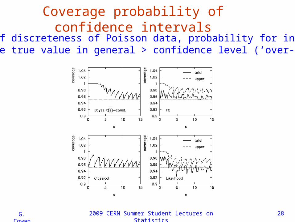
2009 CERN Summer Student Lectures on Statistics 28G. Cowan
Coverage probability of confidence intervalsBecause of discreteness of Poisson data, probability for intervalto include true value in general > confidence level (‘over-coverage’)
2009 CERN Summer Student Lectures on Statistics 29G. Cowan
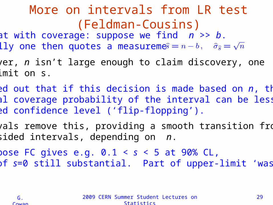
More on intervals from LR test (Feldman-Cousins)
Caveat with coverage: suppose we find n >> b.Usually one then quotes a measurement:
If, however, n isn’t large enough to claim discovery, onesets a limit on s.
FC pointed out that if this decision is made based on n, thenthe actual coverage probability of the interval can be less thanthe stated confidence level (‘flip-flopping’).
FC intervals remove this, providing a smooth transition from1- to 2-sided intervals, depending on n.
But, suppose FC gives e.g. 0.1 < s < 5 at 90% CL, p-value of s=0 still substantial. Part of upper-limit ‘wasted’?
2009 CERN Summer Student Lectures on Statistics 30G. Cowan
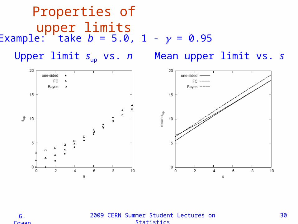
Properties of upper limits
Upper limit sup vs. n Mean upper limit vs. s
Example: take b = 5.0, 1 - = 0.95
2009 CERN Summer Student Lectures on Statistics 31G. Cowan
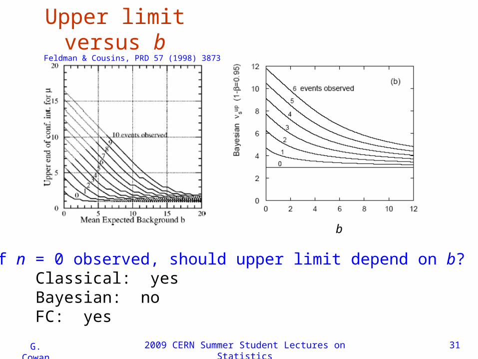
Upper limit versus b
b
If n = 0 observed, should upper limit depend on b?Classical: yesBayesian: noFC: yes
Feldman & Cousins, PRD 57 (1998) 3873