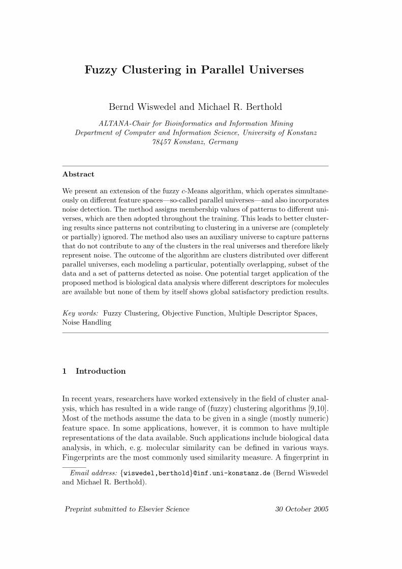
Fuzzy Clustering in Parallel Universes

Bernd Wiswedel and Michael R. Berthold

ALTANA-Chair for Bioinformatics and Information MiningDepartment of Computer and Information Science, University of Konstanz

78457 Konstanz, Germany

Abstract

We present an extension of the fuzzy c-Means algorithm, which operates simultane-ously on different feature spaces—so-called parallel universes—and also incorporatesnoise detection. The method assigns membership values of patterns to different uni-verses, which are then adopted throughout the training. This leads to better cluster-ing results since patterns not contributing to clustering in a universe are (completelyor partially) ignored. The method also uses an auxiliary universe to capture patternsthat do not contribute to any of the clusters in the real universes and therefore likelyrepresent noise. The outcome of the algorithm are clusters distributed over differentparallel universes, each modeling a particular, potentially overlapping, subset of thedata and a set of patterns detected as noise. One potential target application of theproposed method is biological data analysis where different descriptors for moleculesare available but none of them by itself shows global satisfactory prediction results.

Key words: Fuzzy Clustering, Objective Function, Multiple Descriptor Spaces,Noise Handling

1 Introduction

In recent years, researchers have worked extensively in the field of cluster anal-ysis, which has resulted in a wide range of (fuzzy) clustering algorithms [9,10].Most of the methods assume the data to be given in a single (mostly numeric)feature space. In some applications, however, it is common to have multiplerepresentations of the data available. Such applications include biological dataanalysis, in which, e. g. molecular similarity can be defined in various ways.Fingerprints are the most commonly used similarity measure. A fingerprint in

Email address: {wiswedel,berthold}@inf.uni-konstanz.de (Bernd Wiswedeland Michael R. Berthold).

Preprint submitted to Elsevier Science 30 October 2005

a molecular sense is usually a binary vector, whereby each bit indicates thepresence or absence of a molecular feature. The similarity of two compoundscan be expressed based on their bit vectors using the Tanimoto coefficient forexample. Other descriptors encode numerical features derived from 3D maps,incorporating the molecular size and shape, hydrophilic and hydrophobic re-gions quantification, surface charge distribution, etc. [6]. Further similaritiesinvolve the comparison of chemical graphs, inter-atomic distances, and molec-ular field descriptors. However, it has been shown that often a single descriptorfails to show satisfactory prediction results [16].

Other application domains include web mining where a document can be de-scribed based on its content and on anchor texts of hyperlinks pointing to it [4].3D objects as used in CAD-catalogues, virtual reality applications, medicineand many other domains can be described, for instance, by various so-calledfeature vectors, i. e. vector of scalars whose cardinalities can easily reach coupleof hundreds. Feature vectors can rely on different statistics of the 3D object,projection methods, volumetric representations obtained by discretizing theobject’s surface, 2D images, or topological matchings. Bustos et al. [5] providea survey of feature-based similarity measures of 3D objects.

In the following we denote these multiple representations, i. e. different descrip-tor spaces, as Parallel Universes [14], each of which having representations ofall objects of the data set. The challenge that we are facing here is to takeadvantage of the information encoded in the different universes to find clus-ters that reside in one or more universes each modeling one particular subsetof the data. In this paper, we develop an extended fuzzy c-Means (FCM) al-gorithm [1] with noise detection that is applicable to parallel universes, byassigning membership values from objects to universes. The optimization ofthe objective function is similar to the original FCM but also includes thelearning of the membership values to compute the impact of objects to uni-verses.

In the next section, we discuss in more detail the concept of parallel universes;section 3 presents related work. We formulate our new objective function insection 4, introduce the clustering algorithm in section 5 and illustrate itsusefulness with some numeric examples in section 6.

2 Parallel Universes

We consider parallel universes to be a set of feature spaces for a given set ofobjects. Each object is assigned a representation in each single universe. Typ-ically, parallel universes encode different properties of the data and thus leadto different measures of similarity. (For instance, similarity of molecular com-

2

pounds can be based on surface charge distribution or a specific fingerprintrepresentation.) Note, due to these individual measurements they can alsoshow different structural information and therefore exhibit distinctive cluster-ing. This property differs from the problem setting in the so-called Multi-ViewClustering [3] where a single universe, i. e. view, suffices for learning but theaim is on binding different views to improve the classification accuracy and/oraccelerating the learning process.

As it often causes confusion, we want to emphasize the difference of the conceptof parallel universes to feature selection methods [12], feature transformation(such as principle component analysis and singular value decomposition), andsubspace clustering [13,8], whose problem definitions sound similar at firstbut are very different from what we discuss here. Feature selection methodsattempt to discover attributes in a data set that are most relevant to thetask at hand. Subspace clustering is an extension of feature selection thatseeks to identify different subspaces, i. e. subsets of input features, for thesame dataset. These algorithms become particularly useful when dealing withhigh-dimensional data, where often, many dimensions are irrelevant and canmask existing clusters in noise. The main goal of such algorithms is thereforeto uncover subsets of attributes (subspaces), on which subsets of the data areself-similar, i. e. build subspace-clusters, whereas the clustering in parallel uni-verses is given the definition of semantically meaningful universes along withrepresentations of all data in them and the goal is to exploit this information.The objective for our problem definition is on identifying clusters located indifferent universes whereby each cluster models a subset of the data based onsome underlying property.

Since standard clustering techniques are not able to cope with parallel uni-verses, one could either restrict the analysis to a single universe at a timeor define a descriptor space comprising all universes. However, using only oneparticular universe omits information encoded in the other representations andthe construction of a joint feature space and the derivation of an appropriatedistance measure are cumbersome and require great care as it can introduceartifacts or hide and loose clusters that were apparent in a single universe.

3 Related Work

Clustering in parallel universes is a relatively new field of research and was firstmentioned in [14]. In [11], the DBSCAN algorithm is extended and applied toparallel universes. DBSCAN uses the notion of dense regions by means of coreobjects, i. e. objects that have a minimum number k of objects in their (ε-)neighborhood. A cluster is then defined as a set of (connected) dense regions.The authors extend this concept in two different ways: They define an object

3

as a neighbor of a core object if it is in the ε-neighborhood of this core objecteither (1) in any of the representations or (2) in all of them. The cluster sizeis finally determined through appropriate values of ε and k. Case (1) seemsrather weak, having objects in one cluster even though they might not besimilar in any of the representational feature spaces. Case (2), in comparison,is very conservative since it does not reveal local clusters, i. e. subsets of thedata that only group in a single universe. However, the results in [11] arepromising.

Another clustering scheme called “Collaborative fuzzy clustering” is based onthe FCM algorithm and was introduced in [15]. The author proposes an ar-chitecture in which objects described in parallel universes can be processedtogether with the objective of finding structures that are common to all uni-verses. Clustering is carried out by applying the c-Means algorithm to alluniverses individually and then by exchanging information from the local clus-tering results based on the partitioning matrices. Note, the objective function,as introduced in [15], assumes the same number of clusters in each universeand, moreover, a global order on the clusters which is very restrictive due tothe random initialization of FCM.

A supervised clustering technique for parallel universes was given in [14]. It fo-cuses on a model for a particular (minor) class of interest by constructing localneighborhood histograms, so-called Neighborgrams for each object of interestin each universe. The algorithm assigns a quality value to each Neighborgramand greedily includes the best Neighborgram, no matter from which universeit stems, in the global prediction model. Objects that are covered by thisNeighborgram are finally removed from consideration in a sequential coveringmanner. This process is repeated until the global model has sufficient predic-tive power. Although the algorithm is powerful to model a minority class, itsuffers from computational complexity on larger data sets.

Blum and Mitchell [4] introduced co-training as a semi-supervised procedurewhereby two different hypotheses are trained on two distinct representationsand then bootstrap each other. In particular they consider the problem ofclassifying web pages based on the document itself and on anchor texts of in-bound hyperlinks. They require a conditional independence of both universesand state that each representation should suffice for learning if enough labeleddata were available. The benefit of their strategy is that (inexpensive) unla-beled data augment the (expensive) labeled data by using the prediction inone universe to support the decision making in the other.

Other related work includes reinforcement clustering [18] and extensions ofpartitioning methods—such as k-Means, k-Medoids, and EM—and hierarchi-cal, agglomerative methods, all in [3].

4

4 Objective Functions

In this section, we introduce all necessary notation, review the FCM [1,7]algorithm and formulate two new objective functions that are suitable to beused for parallel universes. The first one is a generic function that, similarto the standard FCM, has no explicit noise handling and therefore forces acluster membership prediction for each pattern while the second objectivefunction also incorporates noise detection and, hence, allows patterns to notparticipate to any cluster. The technical details, i. e. the derivation of theobjective functions, can be found in the appendix.

In the following, we consider U , 1 ≤ u ≤ U , parallel universe, each having rep-resentational feature vectors for all objects ~x

(u)i = (x

(u)i,1 , . . . , xu

i,a, . . . xui,Au

) withAu indicating the dimensionality of the u-th universe. We depict the overallnumber of objects as |T |, 1 ≤ i ≤ |T |. We are interested in identifying Ku clus-ters in universe u. We further assume appropriate definitions of distance func-

tions for each universe d(u)(~w

(u)k , ~x

(u)i

)2where ~w

(u)k = (~w

(u)k,1 , . . . , ~w

(u)k,a, . . . ~w

(u)k,Au

)denotes the k-th prototype in the u-th universe.

We confine ourselves to the Euclidean distance in the following. In general,there are no restrictions to the distance metrics other than differentiability. Inparticular, they do not need to be of the same type in all universes. This isimportant to note, since we can use the proposed algorithm in the same featurespace, i. e. ~x

(u1)i = ~x

(u2)i for some u1 and u2, but different distance measures in

these universes.

4.1 Objective Function with No Noise Detection

The standard FCM algorithm relies on one feature space only and minimizesthe accumulated sum of distances between patterns ~xi and cluster centers ~wk,weighted by the degree of membership to which a pattern belongs to a cluster.Note that we omit the subscript u here, as we consider only one universe:

Jm =|T |∑i=1

K∑k=1

vmi,k d (~wk, ~xi)

2 . (1)

The coefficient m ∈ (1,∞) is a fuzzyfication parameter, and vi,k the respectivevalue from the partition matrix, i. e. the degree to which pattern ~xi belongsto cluster k.

5

This function is subject to minimization under the constraint

∀ i :K∑

k=1

vi,k = 1 , (2)

requiring that the coverage of any pattern i needs to accumulate to 1.

The above objective function assumes all cluster candidates to be locatedin the same feature space and is therefore not directly applicable to paralleluniverses. To overcome this, we introduce a matrix (zi,u)1≤i≤|T |,1≤u≤U encodingthe membership of patterns to universes. A value zi,u close to 1 denotes a strongcontribution of pattern ~xi to the clustering in universe u, and a smaller value,a respectively lesser degree.

The new objective function is given by

Jm,m′ =|T |∑i=1

U∑u=1

(zi,u)m′

Ku∑k=1

(v

(u)i,k

)md(u)

(~w

(u)k , ~x

(u)i

)2(3)

Parameter m′ ∈ (1,∞) allows (analogous to m) to have impact on the fuzzyfi-cation of zi,u: The larger m′, the more equal the distribution of zi,u, giving eachpattern an equal impact to all universes. A value close to 1 will strengthen thecomposition of zi,u and assign high values to universes where a pattern showsgood clustering behavior and small values to those where it does not. Note,we now have U , 1 ≤ u ≤ U , different partition matrices

(v

(u)i,k

)1≤i≤|T |,1≤k≤Ku

to

assign membership degrees of objects to cluster prototypes in each universe.

As in the standard FCM algorithm, the objective function has to fulfill sideconstraints. The coverage of a pattern among the partitions in each universemust accumulate to 1:

∀ i, u :Ku∑k=1

v(u)i,k = 1 . (4)

This is similar to the constraint of the single universe FCM in (2) and isrequired for each universe individually.

Additionally, the membership of a pattern to different universes zi,u has tosatisfy standard requirements for membership degrees: it must accumulateto 1 for each object considering all universes and must be in the unit interval,i. e.

∀ i :U∑

u=1

zi,u = 1 . (5)

6

The minimization is done with respect to the parameters v(u)i,k , zi,u, and ~w

(u)k .

The derivation of objective function (3) can be found in the appendix, thefinal update equations are given by (A.12), (A.7), and (A.14).

4.2 Objective Function with Noise Detection

The objective function as introduced in the previous section has one majordrawback: Patterns that do not contribute to any of the clusters in any uni-verse still have a great impact on the cluster formation as the cluster member-ships for each individual pattern need to sum to one. This is not advantageoussince data sets in many real world applications, if not all, contain outliers ornoisy patterns. Particularly in the presented application domain it may hap-pen that certain structural properties of the data are not captured by any ofthe given (semantically meaningful!) universes and therefore this portion ofthe data appears to be noise. The identification of these patterns is importantfor two reasons: First, as noted above, these patterns influence the cluster for-mation and can lead to distorted clusters. Secondly, noise patterns may leadto insights on which properties of the underlying data are not well modeledby any of the universe definitions and therefore give hints as to what needs tobe addressed when defining new universes or similarity measures.

In order to incorporate noise detection we need to extend our objective func-tion such that it also allows the explicit notion of noise. We adopt an extensionintroduced by Dave [7], which works on the single universe FCM. The objec-tive function according to Dave is given by:

Jm =|T |∑i=1

K∑k=1

vmi,k d (~wk, ~xi)

2 + dnoise

|T |∑i=1

(1−

K∑k=1

vi,k

)m

. (6)

This equation is similar to (1) except for the last term. It serves as a noisecluster; all objects have a fixed, user-defined distance dnoise to this noise cluster.Objects that are not close to any cluster center ~wk can therefore be detectedas noise. The constraint (2) must be soften:

∀ i :K∑

k=1

vi,k ≤ 1 , (7)

requiring that the coverage of any pattern i needs to accumulate to at most 1(the remainder to 1 represents the membership to the noise cluster).

Similar to the last term in (6), we add a new term to our new objective func-tion (3) whose role is to “localize” the noise and place it in a single auxiliary

7

universe:

Jm,m′ =|T |∑i=1

U∑u=1

(zi,u)m′

Ku∑k=1

(v

(u)i,k

)md(u)

(~w

(u)k , ~x

(u)i

)2(8)

+ dnoise

|T |∑i=1

(1−

U∑u=1

zi,u

)m′

.

By assigning patterns to this noise universe, we declare them to be outliersin the data set. The parameter dnoise reflects the fixed distance between avirtual cluster in the noise universe and all data points. Hence, if the minimumdistance between a data point and any cluster in one of the universes is greaterthan dnoise, the pattern is labeled as noise.

The optimization splits into three parts: optimization of the partition valuesv

(u)i,k for each universe; determining the membership degrees of patterns to

universes zi,u and finally the adaption of the center vectors of the cluster

representatives ~w(u)k .

The update equations of these parameters are given as follows. For the parti-tion values vi,k, we get

v(u)i,k =

1

Ku∑k=1

d(u)

(~w

(u)k

,~x(u)i

)2

d(u)

(~w

(u)

k,~x

(u)i

)2

1

m−1

. (9)

Note, this equation is independent of the values zi,u and is therefore identicalto the update expression in the single universe FCM. The optimization withrespect to zi,u yields

zi,u =1

U∑u=1

∑Kuk=1

(v(u)i,k

)m

d(u)

(~w

(u)k

,~x(u)i

)2

∑Kuk=1

(v(u)i,k

)m

d(u)

(~w

(u)k

,~x(u)i

)2

+dnoise

1

m′−1

, (10)

and finally the update equation for the adaption of the prototype vectors ~w(u)k

is of the form

~w(u)k =

∑|T |i=1 (zi,u)

m′ (v

(u)i,k

)m~x

(u)i∑|T |

i=1 (zi,u)m′ (

v(u)i,k

)m . (11)

8

Thus, the update of the prototypes depends not only on the partitioning valuev

(u)i,k , i. e. the degree to which pattern i belongs to cluster k in universe u, but

also to zi,u representing the membership degrees of patterns to the currentuniverse of interest. Patterns with larger values zi,u will contribute more tothe adaption of the prototype vectors, while patterns with a smaller degreeaccordingly to a lesser extent.

Equipped with these update equations, we can introduce the overall clusteringscheme in the next section.

5 Clustering algorithm

Similar to the standard FCM algorithm, clustering is carried out in an iterativemanner, involving three steps:

(1) Update of the partition matrices (v(u)i,k )

(2) Update of the membership degrees (zi,u)

(3) Update of the prototypes (~w(u)k )

More precisely, the clustering procedure is given as:

(1) Given: Input pattern set described in U parallel universes: ~x(u)i , 1 ≤

i ≤ |T |, 1 ≤ u ≤ U .

(2) Select: A set of distance metrics d(u) (·, ·)2, and the number of clustersfor each universe Ku, 1 ≤ u ≤ U , define parameter m and m′.

(3) Initialize: Partition parameters v(u)i,k with random values and the cluster

prototypes by drawing samples from the data. Assign equal weights toall membership degrees zi,u = 1

U.

(4) Train:

(5) Repeat

(6) Update partitioning values v(u)i,k according to (9)

(7) Update membership degrees zi,u according to (10)

(8) Compute prototypes ~w(u)i using (11)

(9) until a termination criterion has been satisfied.

The algorithm starts with a given set of universe definitions and the speci-fication of the distance metrics to be used. Also, the number of clusters ineach universe needs to be defined in advance. The membership degrees zi,u

are initialized with equal weight (line (3)), thus having the same impact on

9

all universes. The optimization phase in line (5) to (9) is—in comparison tothe standard FCM algorithm—extended by the optimization of the universemembership degrees, line (7). The possibilities for the termination criterionin line (9) are manifold, as is also the case in the standard FCM. One canstop after a certain number of iterations or use the change of the value of theobjective function (3) between two successive iterations as stopping criteria.There are also more sophisticated approaches, for instance the change to thepartition matrices during optimization.

Just like the FCM algorithm, this method suffers from the fact that the userhas to specify the number of prototypes to be found. Furthermore, our ap-proach even requires the definition of cluster counts per universe. There arenumerous approaches to suggest the number of clusters in the case of thestandard FCM, [19,17,2] to name but a few. Although we have not yet stud-ied their applicability to our problem definition we do believe that some ofthem can be adapted naturally to be used in our context as well.

6 Experimental Results

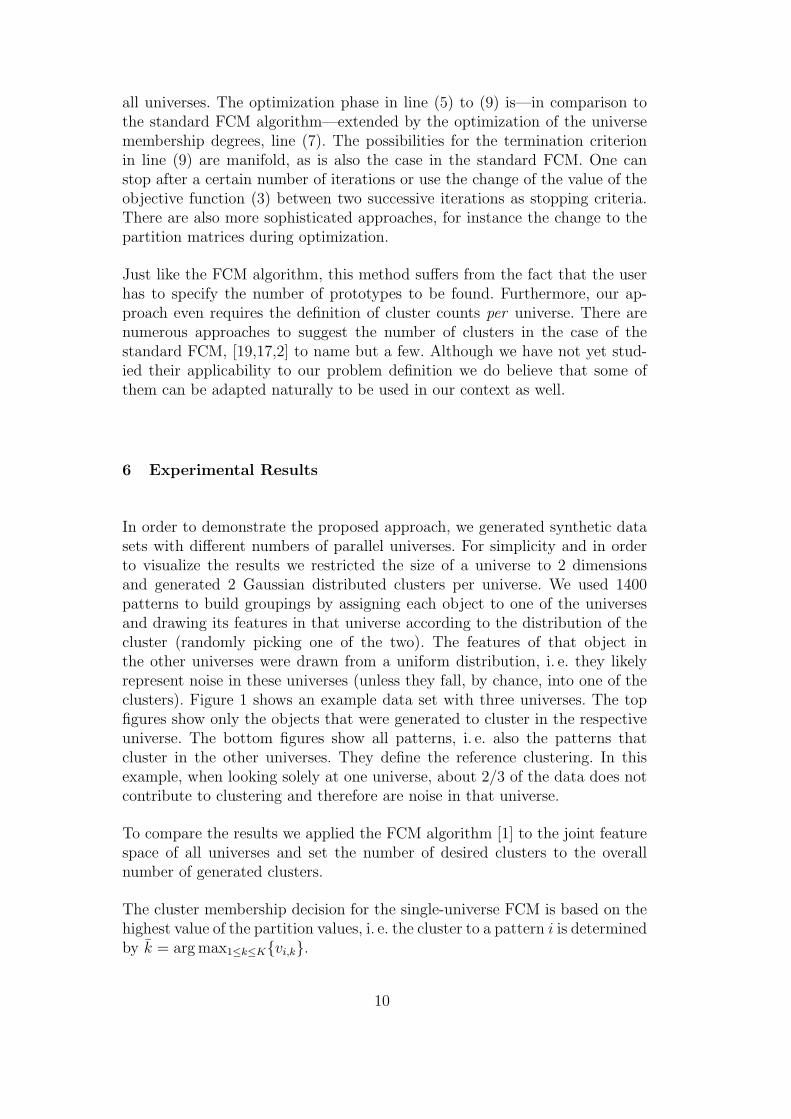
In order to demonstrate the proposed approach, we generated synthetic datasets with different numbers of parallel universes. For simplicity and in orderto visualize the results we restricted the size of a universe to 2 dimensionsand generated 2 Gaussian distributed clusters per universe. We used 1400patterns to build groupings by assigning each object to one of the universesand drawing its features in that universe according to the distribution of thecluster (randomly picking one of the two). The features of that object inthe other universes were drawn from a uniform distribution, i. e. they likelyrepresent noise in these universes (unless they fall, by chance, into one of theclusters). Figure 1 shows an example data set with three universes. The topfigures show only the objects that were generated to cluster in the respectiveuniverse. The bottom figures show all patterns, i. e. also the patterns thatcluster in the other universes. They define the reference clustering. In thisexample, when looking solely at one universe, about 2/3 of the data does notcontribute to clustering and therefore are noise in that universe.

To compare the results we applied the FCM algorithm [1] to the joint featurespace of all universes and set the number of desired clusters to the overallnumber of generated clusters.

The cluster membership decision for the single-universe FCM is based on thehighest value of the partition values, i. e. the cluster to a pattern i is determinedby k = arg max1≤k≤K{vi,k}.

10

0

0.2

0.4

0.6

0.8

1

0 0.2 0.4 0.6 0.8 1

Universe 1

0

0.2

0.4

0.6

0.8

1

0 0.2 0.4 0.6 0.8 1

Universe 2

0

0.2

0.4

0.6

0.8

1

0 0.2 0.4 0.6 0.8 1

Universe 3

0

0.2

0.4

0.6

0.8

1

0 0.2 0.4 0.6 0.8 1

0

0.2

0.4

0.6

0.8

1

0 0.2 0.4 0.6 0.8 1

0

0.2

0.4

0.6

0.8

1

0 0.2 0.4 0.6 0.8 1

Fig. 1. Three universes of a synthetic data set. The top figures show only objectsthat were generated within the respective universe (using two clusters per universe).The bottom figures show all patterns; note that most of them (i. e. the ones fromthe other two universes), are noise in this particular universe. For clarification weuse different shapes for objects that originate from different universes.

Fig. 2. Clustering quality for 3 different data sets. The number of universes rangesfrom 2 to 4 universes. Note how the cluster quality of the joint feature space dropssharply whereas the parallel universe approach seems less affected. An overall declineof cluster quality is to be expected since the number of clusters to be detectedincreases.

When the universe information is taken into account, a cluster decision isbased on the memberships to universes zi,u and memberships to clusters v

(u)i,k .

The “winning” universe is determined by u = arg max1≤u≤U{zi,u} and the

corresponding cluster in u is calculated as k = arg max1≤k≤Ku{v(u)i,k }.

We used the following quality measure to evaluate the clustering outcome and

11

compare it to the reference clustering [11]:

QK(C) =∑

Ci∈C

|Ci||T |

· (1− entropyK(Ci)) ,

where K is the reference clustering, i. e. the clusters as generated, C the clus-tering to evaluate, and entropyK(Ci) the entropy of cluster Ci with respect toK. This function is 1 if C equals K and 0 if all clusters are completely mixedsuch that they all contain an equal fraction of the clusters in K or all pointsare predicted to be noise. Thus, the higher the value, the better the clustering.

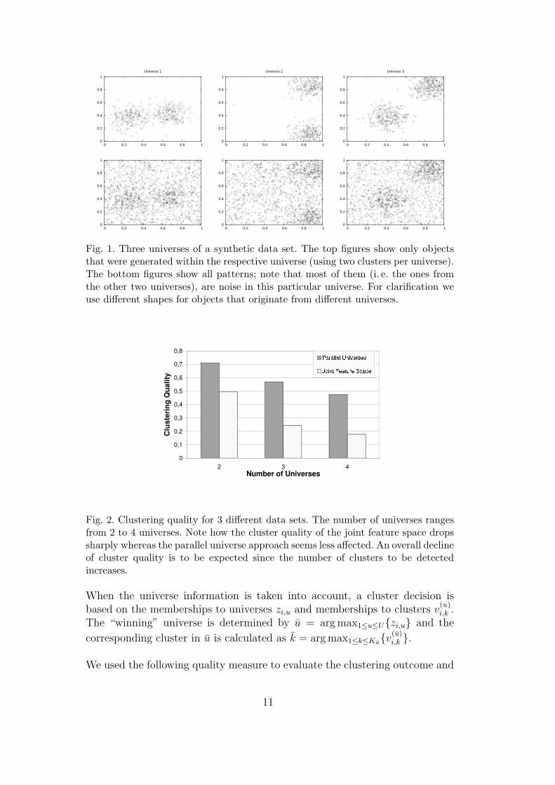
Figure 2 summarizes the quality values for 3 experiments. The number ofuniverses ranges from 2 to 4. The left bar for each experiment in figure 2shows the quality value when using the new objective function as introduced insection 4.1, i. e. with incorporating the knowledge of parallel universes but noexplicit noise detection. The right bar shows the quality value when applyingthe standard FCM to the joint feature space. Clearly, for this data set, ouralgorithm takes advantage of the information encoded in different universesand identifies the major parts of the original clusters much better.

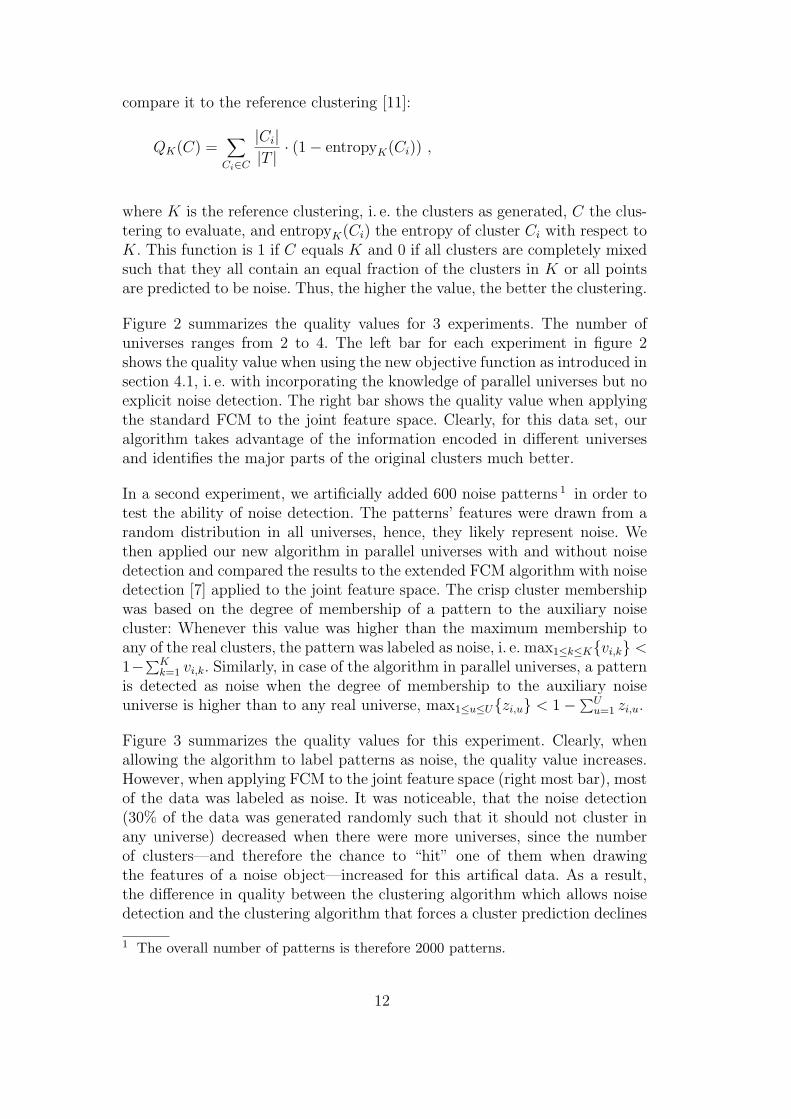
In a second experiment, we artificially added 600 noise patterns 1 in order totest the ability of noise detection. The patterns’ features were drawn from arandom distribution in all universes, hence, they likely represent noise. Wethen applied our new algorithm in parallel universes with and without noisedetection and compared the results to the extended FCM algorithm with noisedetection [7] applied to the joint feature space. The crisp cluster membershipwas based on the degree of membership of a pattern to the auxiliary noisecluster: Whenever this value was higher than the maximum membership toany of the real clusters, the pattern was labeled as noise, i. e. max1≤k≤K{vi,k} <1−∑K

k=1 vi,k. Similarly, in case of the algorithm in parallel universes, a patternis detected as noise when the degree of membership to the auxiliary noiseuniverse is higher than to any real universe, max1≤u≤U{zi,u} < 1−∑U

u=1 zi,u.

Figure 3 summarizes the quality values for this experiment. Clearly, whenallowing the algorithm to label patterns as noise, the quality value increases.However, when applying FCM to the joint feature space (right most bar), mostof the data was labeled as noise. It was noticeable, that the noise detection(30% of the data was generated randomly such that it should not cluster inany universe) decreased when there were more universes, since the numberof clusters—and therefore the chance to “hit” one of them when drawingthe features of a noise object—increased for this artifical data. As a result,the difference in quality between the clustering algorithm which allows noisedetection and the clustering algorithm that forces a cluster prediction declines

1 The overall number of patterns is therefore 2000 patterns.

12

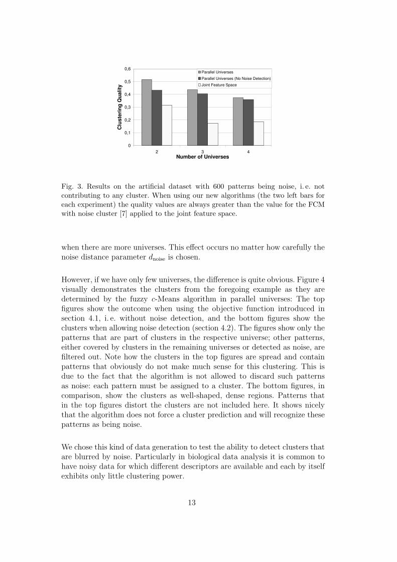
Fig. 3. Results on the artificial dataset with 600 patterns being noise, i. e. notcontributing to any cluster. When using our new algorithms (the two left bars foreach experiment) the quality values are always greater than the value for the FCMwith noise cluster [7] applied to the joint feature space.

when there are more universes. This effect occurs no matter how carefully thenoise distance parameter dnoise is chosen.

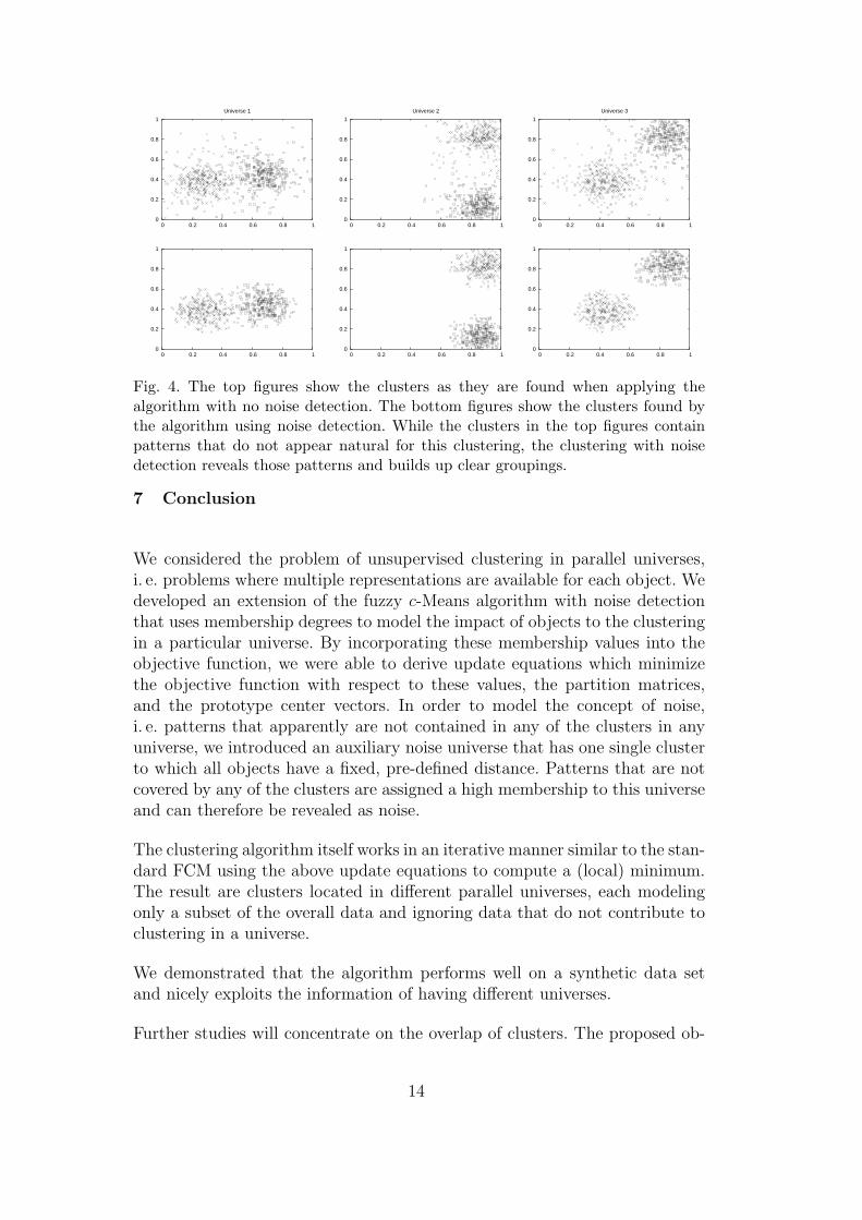
However, if we have only few universes, the difference is quite obvious. Figure 4visually demonstrates the clusters from the foregoing example as they aredetermined by the fuzzy c-Means algorithm in parallel universes: The topfigures show the outcome when using the objective function introduced insection 4.1, i. e. without noise detection, and the bottom figures show theclusters when allowing noise detection (section 4.2). The figures show only thepatterns that are part of clusters in the respective universe; other patterns,either covered by clusters in the remaining universes or detected as noise, arefiltered out. Note how the clusters in the top figures are spread and containpatterns that obviously do not make much sense for this clustering. This isdue to the fact that the algorithm is not allowed to discard such patternsas noise: each pattern must be assigned to a cluster. The bottom figures, incomparison, show the clusters as well-shaped, dense regions. Patterns thatin the top figures distort the clusters are not included here. It shows nicelythat the algorithm does not force a cluster prediction and will recognize thesepatterns as being noise.

We chose this kind of data generation to test the ability to detect clusters thatare blurred by noise. Particularly in biological data analysis it is common tohave noisy data for which different descriptors are available and each by itselfexhibits only little clustering power.

13

0

0.2

0.4

0.6

0.8

1

0 0.2 0.4 0.6 0.8 1

Universe 1

0

0.2

0.4

0.6

0.8

1

0 0.2 0.4 0.6 0.8 1

Universe 2

0

0.2

0.4

0.6

0.8

1

0 0.2 0.4 0.6 0.8 1

Universe 3

0

0.2

0.4

0.6

0.8

1

0 0.2 0.4 0.6 0.8 1

0

0.2

0.4

0.6

0.8

1

0 0.2 0.4 0.6 0.8 1

0

0.2

0.4

0.6

0.8

1

0 0.2 0.4 0.6 0.8 1

Fig. 4. The top figures show the clusters as they are found when applying thealgorithm with no noise detection. The bottom figures show the clusters found bythe algorithm using noise detection. While the clusters in the top figures containpatterns that do not appear natural for this clustering, the clustering with noisedetection reveals those patterns and builds up clear groupings.

7 Conclusion

We considered the problem of unsupervised clustering in parallel universes,i. e. problems where multiple representations are available for each object. Wedeveloped an extension of the fuzzy c-Means algorithm with noise detectionthat uses membership degrees to model the impact of objects to the clusteringin a particular universe. By incorporating these membership values into theobjective function, we were able to derive update equations which minimizethe objective function with respect to these values, the partition matrices,and the prototype center vectors. In order to model the concept of noise,i. e. patterns that apparently are not contained in any of the clusters in anyuniverse, we introduced an auxiliary noise universe that has one single clusterto which all objects have a fixed, pre-defined distance. Patterns that are notcovered by any of the clusters are assigned a high membership to this universeand can therefore be revealed as noise.

The clustering algorithm itself works in an iterative manner similar to the stan-dard FCM using the above update equations to compute a (local) minimum.The result are clusters located in different parallel universes, each modelingonly a subset of the overall data and ignoring data that do not contribute toclustering in a universe.

We demonstrated that the algorithm performs well on a synthetic data setand nicely exploits the information of having different universes.

Further studies will concentrate on the overlap of clusters. The proposed ob-

14

jective function rewards clusters that only occur in one universe. Objects thatcluster well in more than one universe could possibly be identified when havingbalanced membership values to the universes but very unbalanced partitioningvalues for the cluster memberships within these particular universes.

Other studies will continue to focus on the applicability of the proposedmethod to real world data and heuristics that adjust the number of clustersper universe.

Acknowledgments

This work was partially supported by DFG Research Training Group GK-1042“Explorative Analysis and Visualization of Large Information Spaces”.

A Appendix

In order to compute a minimum of the objective function (3) with respectto (4) and (5), we exploit a Lagrange technique to merge the constrained partof the optimization problem with the unconstrained one. Note, we skip theextra notation of the noise universe in (8); it can be seen as an additionaluniverse, i. e. the number of universe is U + 1, that has one cluster to whichall patterns have a fixed distance of dnoise. The derivation can then be appliedas follows.

It leads to a new objective function Fi

Fi =U∑

u=1

(zi,u)m′

Ku∑k=1

(v

(u)i,k

)md(u)

(~w

(u)k , ~x

(u)i

)2(A.1)

+U∑

u=1

λ′u

(1−

Ku∑k=1

v(u)i,k

)+ λ

(1−

U∑u=1

zi,u

),

which we minimize individually for each pattern ~xi. The parameters λ and λ′u,1 ≤ u ≤ U , denote the Lagrange multipliers to take (4) and (5) into account.The necessary conditions leading to local minima of Fi read as

∂Fi

∂zi,u

= 0,∂Fi

∂v(u)i,k

= 0,∂Fi

∂λ= 0,

∂Fi

∂λ′u= 0 , (A.2)

1 ≤ u ≤ U, 1 ≤ k ≤ Ku.

15

In the following we will derive update equations for the z and v parameters.Evaluating the first derivative of the equations in (A.2) yields the expression

∂Fi

∂zi,u

= m′ (zi,u)m′−1

Ku∑k=1

(v

(u)i,k

)md(u)

(~w

(u)k , ~x

(u)i

)2− λ = 0,

and hence

zi,u =

(λ

m′

) 1m′−1

1∑Kuk=1

(v

(u)i,k

)md(u)

(~w

(u)k , ~x

(u)i

)2

1

m′−1

. (A.3)

We can rewrite the above equation

(λ

m′

) 1m′−1

= zi,u

(Ku∑k=1

(v

(u)i,k

)md(u)

(~w

(u)k , ~x

(u)i

)2) 1

m′−1

. (A.4)

From the derivative of Fi w. r. t. λ in (A.2), it follows

∂Fi

∂λ= 1−

U∑u=1

zi,u = 0

U∑u=1

zi,u = 1 , (A.5)

which returns the normalization condition as in (5). Using the formula for zi,u

in (A.3) and integrating it into expression (A.5) we compute

U∑u=1

(λ

m′

) 1m′−1

1∑Kuk=1

(v

(u)i,k

)md(u)

(~w

(u)k , ~x

(u)i

)2

1

m′−1

= 1

(λ

m′

) 1m′−1 U∑

u=1

1∑Kuk=1

(v

(u)i,k

)md(u)

(~w

(u)k , ~x

(u)i

)2

1

m′−1

= 1. (A.6)

We make use of (A.4) and substitute(

λm′

) 1m′−1 in (A.6). Note, we use u as

parameter index of the sum to address the fact that it covers all universes,whereas u denotes the current universe of interest. It follows

1 = zi,u

(Ku∑k=1

(v

(u)i,k

)md(u)

(~w

(u)k , ~x

(u)i

)2) 1

m′−1

16

·U∑

u=1

1∑Kuk=1

(v

(u)i,k

)md(u)

(~w

(u)k , ~x

(u)i

)2

1

m′−1

,

which can be simplified to

1 = zi,u

U∑u=1

∑Ku

k=1

(v

(u)i,k

)md(u)

(~w

(u)k , ~x

(u)i

)2

∑Kuk=1

(v

(u)i,k

)md(u)

(~w

(u)k , ~x

(u)i

)2

1

m′−1

,

and returns an immediate update expression for the membership zi,u of patterni to universe u:

zi,u =1

U∑u=1

∑Kuk=1

(v(u)i,k

)m

d(u)

(~w

(u)k

,~x(u)i

)2

∑Kuk=1

(v(u)i,k

)m

d(u)

(~w

(u)k

,~x(u)i

)2

1

m′−1

. (A.7)

Analogous to the calculations above we can derive the update equation forvalue v

(u)i,k which represents the partitioning value of pattern i to cluster k in

universe u. From (A.2) it follows

∂Fi

∂v(u)i,k

= (zi,u)m′

m(v

(u)i,k

)m−1d(u)

(~w

(u)k , ~x

(u)i

)2− λ′u = 0,

and thus

v(u)i,k =

λ′u

m (zi,u)m′

d(u)(~w

(u)k , ~x

(u)i

)2

1

m−1

, (A.8)

(λ′u

m (zi,u)m′

) 1m−1

= v(u)i,k

(d(u)

(~w

(u)k , ~x

(u)i

)2) 1

m−1

. (A.9)

Zeroing the derivative of Fi w. r. t. λ′u will result in condition (4), ensuringthat the partition values sum to 1, i. e.

∂Fi

∂λ′u= 1−

Ku∑k=1

v(u)i,k = 0 . (A.10)

We use (A.8) and (A.10) to come up with

17

1 =Ku∑k=1

λ′u

m (zi,u)m′

d(u)(~w

(u)k , ~x

(u)i

)2

1

m−1

,

1 =

(λ′u

m (zi,u)m′

) 1m−1 Ku∑

k=1

1

d(u)(~w

(u)k , ~x

(u)i

)2

1

m−1

. (A.11)

Equation (A.9) allows us to replace the first multiplier in (A.11). We will usethe k notation to point out that the sum in (A.11) considers all partitions ina universe and k to denote one particular cluster coming from (A.8),

1 = v(u)i,k

(d(u)

(~w

(u)k , ~x

(u)i

)2) 1

m−1

·Ku∑k=1

1

d(u)(~w

(u)

k, ~x

(u)i

)2

1

m−1

1 = v(u)i,k

Ku∑k=1

d(u)(~w

(u)k , ~x

(u)i

)2

d(u)(~w

(u)

k, ~x

(u)i

)2

1

m−1

Finally, the update rule for v(u)i,k arises as:

v(u)i,k =

1

Ku∑k=1

d(u)

(~w

(u)k

,~x(u)i

)2

d(u)

(~w

(u)

k,~x

(u)i

)2

1

m−1

. (A.12)

For the sake of completeness we also derive the update rules for the clusterprototypes ~w

(u)k . We confine ourselves to the Euclidean distance here, assuming

the data is normalized 2 :

d(u)(~w

(u)k , ~x

(u)i

)2=

Au∑a=1

(w

(u)k,a − x

(u)i,a

)2, (A.13)

with Au the number of dimensions in universe u and w(u)k,a the value of the

prototype in dimension a. x(u)i,a is the value of the a-th attribute of pattern

i in universe u, respectively. The necessary condition for a minimum of theobjective function (3) is of the form ∇

~w(u)k

J = 0. Using the Euclidean distance

as given in (A.13) we obtain

2 The derivation of the updates using other than the Euclidean distance works ina similar manner.

18

∂Jm,m′

∂w(u)k,a

!= 0

2|T |∑i=1

(zi,u)m′ (

v(u)i,k

)m (w

(u)k,a − x

(u)i,a

)= 0

w(u)k,a

|T |∑i=1

(zi,u)m′ (

v(u)i,k

)m=

|T |∑i=1

(zi,u)m′ (

v(u)i,k

)mx

(u)i,a

w(u)k,a =

∑|T |i=1 (zi,u)

m′ (v

(u)i,k

)mx

(u)i,a∑|T |

i=1 (zi,u)m′ (

v(u)i,k

)m . (A.14)

References

[1] J. C. Bezdek. Pattern Recognition with Fuzzy Objective Function Algorithms.Plenum Press, New York, 1981.

[2] James C. Bezdek and Richard J. Hathaway. VAT: a tool for visual assessmentof (cluster) tendency. In Proceedings of the 2002 International Joint Conferenceon Neural Networks (IJCNN ’02), pages 2225–2230, 2002.

[3] Steffen Bickel and Tobias Scheffer. Multi-view clustering. In Proceedings ofthe Fourth IEEE International Conference on Data Mining (ICDM’04), pages19–26, 2004.

[4] Avrim Blum and Tom Mitchell. Combining labeled and unlabeled data withco-training. In Proceedings of the eleventh annual Conference on ComputationalLearning Theory (COLT’98), pages 92–100. ACM Press, 1998.

[5] Benjamin Bustos, Daniel A. Keim, Dietmar Saupe, Tobias Schreck, andDejan V. Vranic. An experimental effectiveness comparison of methods for3D similarity search. International Journal on Digital Libraries, Special issueon Multimedia Contents and Management in Digital Libraries, 2005. To appear.

[6] G. Cruciani, P. Crivori, P.-A. Carrupt, and B. Testa. Molecular fields inquantitative structure-permeation relationships: the VolSurf approach. Journalof Molecular Structure, 503:17–30, 2000.

[7] Rajesh N. Dave. Characterization and detection of noise in clustering. PatternRecognition Letters, 12:657–664, 1991.

[8] Jerome H. Friedman and Jacqueline J. Meulmany. Clustering objects on subsetsof attributes. Journal of the Royal Statistical Society, 66(4), 2004.

[9] David J. Hand, Heikki Mannila, and Padhraic Smyth. Principles of DataMining. MIT Press, 2001.

[10] Frank Hoppner, Frank Klawoon, Rudolf Kruse, and Thomas Runkler. FuzzyCluster Analysis. John Wiley, Chichester, England, 1999.

19

[11] Karin Kailing, Hans-Peter Kriegel, Alexey Pryakhin, and Matthias Schubert.Clustering multi-represented objects with noise. In PAKDD, pages 394–403,2004.

[12] Huan Liu and Hiroshi Motoda. Feature Selection for Knowledge Discovery &Data Mining. Kluwer Academic Publishers, 1998.

[13] Lance Parsons, Ehtesham Haque, and Huan Liu. Subspace clustering for highdimensional data: a review. SIGKDD Explor. Newsl., 6(1):90–105, 2004.

[14] David E. Patterson and Michael R. Berthold. Clustering in parallel universes.In Proceedings of the 2001 IEEE Conference in Systems, Man and Cybernetics.IEEE Press, 2001.

[15] Witold Pedrycz. Collaborative fuzzy clustering. Pattern Recognition Letters,23(14):1675–1686, 2002.

[16] Ansgar Schuffenhauer, Valerie J. Gillet, and Peter Willett. Similarity searchingin files of three-dimensional chemical structures: Analysis of the bioster databaseusing two-dimensional fingerprints and molecular field descriptors. Journal ofChemical Information and Computer Sciences, 40(2):295–307, 2000.

[17] N. B. Venkateswarlu and P. S. V. S. K. Raju. Fast ISODATA clusteringalgorithms. Pattern Recognition, 25(3):335–342, 1992.

[18] Jidong Wang, Hua-Jun Zeng, Zheng Chen, Hongjun Lu, Li Tao, and Wei-YingMa. ReCoM: Reinforcement clustering of multi-type interrelated data objects.In In Proceedings of the 26th annual international ACM SIGIR conference onresearch and development in information retrieval (SIGIR’03), pages 274–281,2003.

[19] R. R. Yager and D. P. Filev. Approximate clustering via the mountain method.IEEE Trans. Systems Man Cybernet., 24(8):1279–1284, August 1994.

20