FUSION OF ALS POINT CLOUD DATA WITH HIGH PRECISION SURVEYING DATA

A. Wehr a, *, H. Duzelovic b, Ch. Punz b

a Institute of Navigation, University of Stuttgart, Breitscheidstr. 2, 70174 Stuttgart, Germany –

wehr@nav.uni-stuttgart.de b rmDATA, Datenverarbeitungs GmbH, Prinz Eugen-Straße 12, A-7400 Oberwart, Austria –

(duzelovic, punz)@rmdata.at

KEY WORDS: LIDAR, Fusion, Modelling, Algorithms, DEM/DTM, Multisensor ABSTRACT: In today airborne laser scanning (ALS) extended areas are surveyed with a high point density and with decimetre elevation accuracy in a very short time. However, due to the finite sampling process the correct modelling of the surveyed earth surface is difficult, if break lines and special topographic features like railway tracks and highways are to be modelled. To improve the ALS derived models more and more additional surveying data are used which are measured by e.g. GNSS or tacheometers. These measurements have higher accuracy and are sampled in a way that they describe best the features to be modelled. For example break lines are described by splines derived from a tacheometric survey. As these supplement data are provided from independent sensors in their own coordinate system, all data sets to be fused have to be transformed so that the most accurate model can be computed. This means the algorithms must regard data property of the different data sets. In addition the most accurate and precise data set has to be used as reference. In this paper algorithms for the fusion of ALS data and additional surveying data obtained from tacheometric and DGNSS measurements are presented and discussed based on results of empirical computations on different data sets. The additional surveying data consists either of single point measurements or profiles. The presented algorithms are developed under the objective to use primarily existing functionalities of a commercial program

* Corresponding author.

1. INTRODUCTION

Today airborne laser scanning (ALS) makes possible surveying the topography of extended areas with high point density and with decimetre elevation accuracy in a very short time. For example the ALTM Gemini of the Optech company achieves a swath width of 1865 m flying at an altitude of 2000 m and sampling data with a point density of about 1.5 m realizing the mentioned accuracy. Although this advanced technology revolutionized the surveying with regard to the amount of data and elevation accuracy, there is still a deficiency in precise modelling special topographical features, e.g. break lines, highways, railway tracks etc. due to the sampling process. However, very often these special topographical elements are surveyed by distinct surveying means like GNSS and tacheometric measurements, which reach accuracy down to millimetres. Therefore, it is obvious to combine these complementary measurements for an advanced modelling. In addition, it must be regarded that more and more the modelling process using ALS data is supported by using information of geoinformation systems (GIS). Following the trends in generating precise Digital Terrain Models (DTMs) out of ALS data makes clear that all available additional information is integrated into the modelling process to speed up, to improve the robustness of calculations and to increase the precision. This paper deals only with the integration of supporting surveying measurements obtained by conventional means e.g. GNSS real time kinematic and tacheometric measurements. These measurements exhibit in general a much lower point density but offer a point accuracy which is an order of magnitude better compared to ALS data.

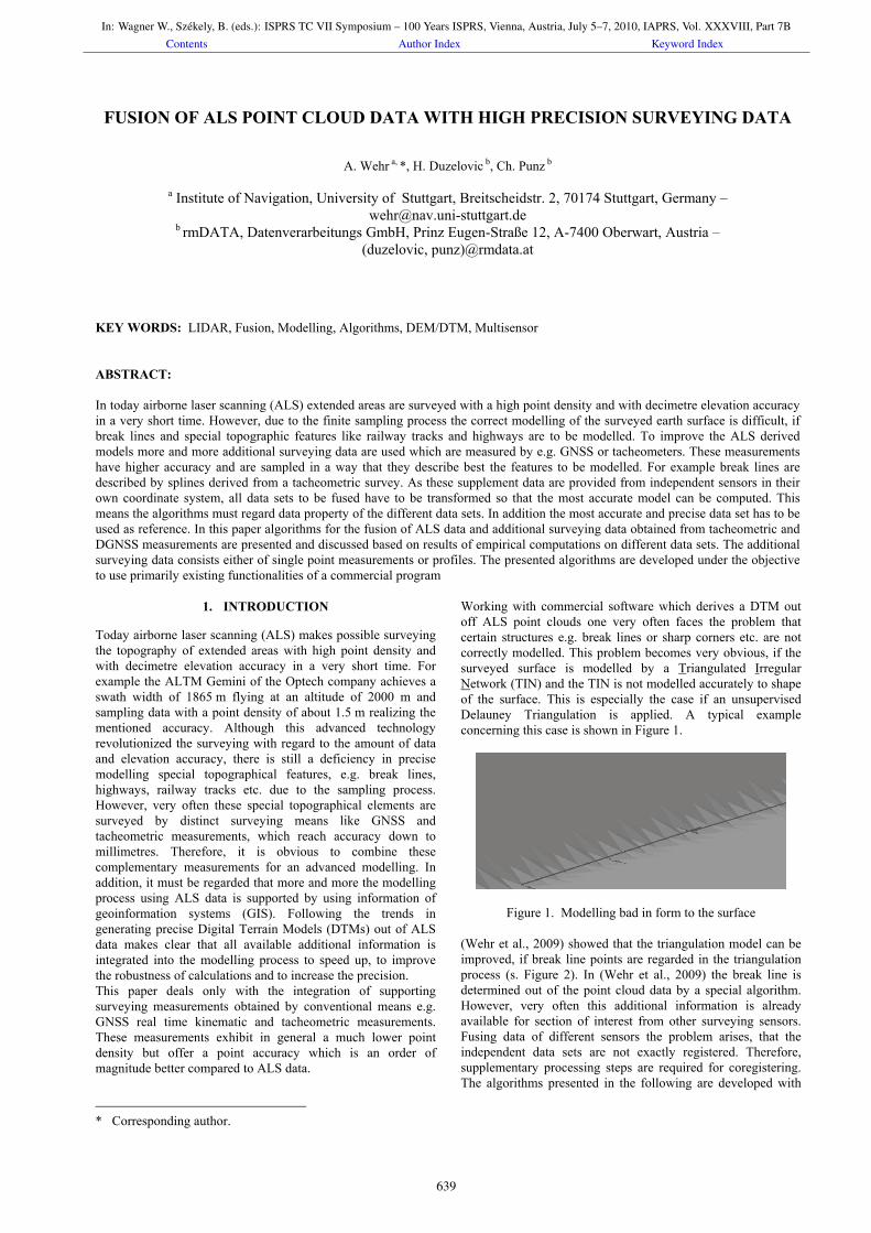
Working with commercial software which derives a DTM out off ALS point clouds one very often faces the problem that certain structures e.g. break lines or sharp corners etc. are not correctly modelled. This problem becomes very obvious, if the surveyed surface is modelled by a Triangulated Irregular Network (TIN) and the TIN is not modelled accurately to shape of the surface. This is especially the case if an unsupervised Delauney Triangulation is applied. A typical example concerning this case is shown in Figure 1.

Figure 1. Modelling bad in form to the surface (Wehr et al., 2009) showed that the triangulation model can be improved, if break line points are regarded in the triangulation process (s. Figure 2). In (Wehr et al., 2009) the break line is determined out of the point cloud data by a special algorithm. However, very often this additional information is already available for section of interest from other surveying sensors. Fusing data of different sensors the problem arises, that the independent data sets are not exactly registered. Therefore, supplementary processing steps are required for coregistering. The algorithms presented in the following are developed with

In: Wagner W., Székely, B. (eds.): ISPRS TC VII Symposium – 100 Years ISPRS, Vienna, Austria, July 5–7, 2010, IAPRS, Vol. XXXVIII, Part 7BContents Author Index Keyword Index

639

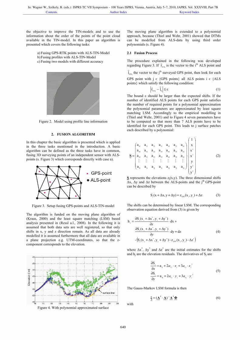
the objective to improve the TIN-models and to use the information about the order of the points of the point cloud available in the TIN-model. In this paper an algorithm is presented which covers the following tasks:

a) Fusing GPS-RTK points with ALS-TIN-Model b) Fusing profiles with ALS-TIN-Model c) Fusing two models with different accuracy

Figure 2. Model using profile line information

2. FUSION ALGORITHM

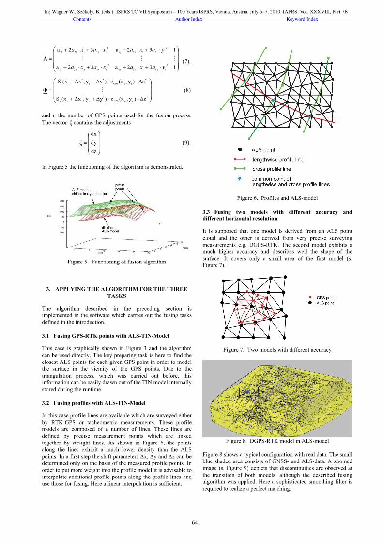
In this chapter the basic algorithm is presented which is applied in the three tasks mentioned in the introduction. A basic algorithm can be defined as the three tasks have in common, fusing 3D surveying points of an independent sensor with ALS-points (s. Figure 3) which corresponds directly with case a).

Figure 3. Setup fusing GPS-points and ALS-TIN-model The algorithm is funded on the moving plane algorithm of (Kraus, 2000) and the least square matching (LSM) based analysis presented in (Ressl a.l., 2008). In the following it is assumed that both data sets are well registered, so that only shifts in x, y and z direction remain. As all data are already modelled it is assumed furthermore that all data are available in a plane projection e.g. UTM-coordinates, so that the z-component corresponds to the elevation.

Figure 4. With polynomial approximated surface

The moving plane algorithm is extended to a polynomial approach, because (Thiel and Wehr, 2001) showed that DTMs can be modelled from ALS-data by using third order polynomials (s. Figure 4). 2.1 Fusion Process

The procedure explained in the following was developed regarding Figure 3. If

iALSrr

is the vector to the ith ALS point and

jGPSlr

the vector to the jth surveyed GPS point, then look for each

GPS point with j є {GPS points} all ALS points i є {ALS points} which satisfy the following condition:

εlrjPiALS ≤−rr

(1)

The bound ε should be larger than the expected shifts. If the number of identified ALS points for each GPS point satisfies the number of required points for a polynomial approximation the polynomial parameters are approximated by least square matching LSM. Accordingly to the empirical modelling in (Thiel and Wehr, 2001) and to Figure 4 seven parameters have to be computed so that more than 7 ALS points have to be identified for each GPS point. This leads to j surface patches each described by a polynomial:

⎟⎟⎟⎟⎟⎟⎟⎟⎟⎟

⎠

⎞

⎜⎜⎜⎜⎜⎜⎜⎜⎜⎜

⎝

⎛

⋅

⎟⎟⎟⎟⎟⎟⎟

⎠

⎞

⎜⎜⎜⎜⎜⎜⎜

⎝

⎛

=

3

2

3

2

6j5j4j3j2j1j0j

63534333231303

62524232221202

61514131211101

yyyxxx1

aaaaaaa

aaaaaaaaaaaaaaaaaaaaa

MMMMMMM

S (2)

S represents the elevations zj(x,y). The three dimensional shifts Δx, Δy and Δz between the ALS-points and the jth GPS-point can be described by Δz)y,(xzΔy)yΔx,(xS jjGPSj +=++ (3) The shifts can be determined by linear LSM. The corresponding observation equation derived from (3) is given by

( )*jjGPS

*j

*jj

*j

*jj

*j

*jj

j

Δz-)y,(xz-)Δyy,Δx(xS-

dz dy )yy,x(xS

dx)yy,x(xS

h

++

+⋅∂

Δ+Δ+∂

+⋅∂

Δ+Δ+∂=

y

x

(4)

where Δx*, Δy* and Δz* are the initial estimates for the shifts and hj are the elevation residuals. The derivatives of Sj are

2

654j

j

2

321j

j

32aS

32a S

jjjj

jjjj

yayay

xaxax

⋅+⋅+=∂∂

⋅+⋅+=∂∂

(5)

The Gauss-Markov LSM formula is then ΦAAAξ TT 1)( −⋅= (6)

with

In: Wagner W., Székely, B. (eds.): ISPRS TC VII Symposium – 100 Years ISPRS, Vienna, Austria, July 5–7, 2010, IAPRS, Vol. XXXVIII, Part 7BContents Author Index Keyword Index

640

⎟⎟⎟⎟

⎠

⎞

⎜⎜⎜⎜

⎝

⎛

⋅+⋅+⋅+⋅+

⋅+⋅+⋅+⋅+=

132a32a

132a32a

2

16154n

2

321n

2

161154j

2

1312111

yaxaxaxa

yaxaxaxa

nnnnnn

jj

MMMA (7),

⎟⎟⎟

⎠

⎞

⎜⎜⎜

⎝

⎛

++

++=Φ

*nnGPS

*n

*nn

*11GPS

*1

*11

Δz-)y,(xz-)Δyy,Δx(xS

Δz-)y,(xz-)Δyy,Δx(xSM (8)

and n the number of GPS points used for the fusion process. The vector ξ contains the adjustments

⎟⎟⎟

⎠

⎞

⎜⎜⎜

⎝

⎛=

dzdydx

ξ (9).

In Figure 5 the functioning of the algorithm is demonstrated.

Figure 5. Functioning of fusion algorithm

3. APPLYING THE ALGORITHM FOR THE THREE TASKS

The algorithm described in the preceding section is implemented in the software which carries out the fusing tasks defined in the introduction. 3.1 Fusing GPS-RTK points with ALS-TIN-Model

This case is graphically shown in Figure 3 and the algorithm can be used directly. The key preparing task is here to find the closest ALS points for each given GPS point in order to model the surface in the vicinity of the GPS points. Due to the triangulation process, which was carried out before, this information can be easily drawn out of the TIN model internally stored during the runtime. 3.2 Fusing profiles with ALS-TIN-Model

In this case profile lines are available which are surveyed either by RTK-GPS or tacheometric measurements. These profile models are composed of a number of lines. These lines are defined by precise measurement points which are linked together by straight lines. As shown in Figure 6, the points along the lines exhibit a much lower density than the ALS points. In a first step the shift parameters Δx, Δy and Δz can be determined only on the basis of the measured profile points. In order to put more weight into the profile model it is advisable to interpolate additional profile points along the profile lines and use those for fusing. Here a linear interpolation is sufficient.

Figure 6. Profiles and ALS-model 3.3 Fusing two models with different accuracy and different horizontal resolution

It is supposed that one model is derived from an ALS point cloud and the other is derived from very precise surveying measurements e.g. DGPS-RTK. The second model exhibits a much higher accuracy and describes well the shape of the surface. It covers only a small area of the first model (s. Figure 7).

Figure 7. Two models with different accuracy

Figure 8. DGPS-RTK model in ALS-model

Figure 8 shows a typical configuration with real data. The small blue shaded area consists of GNSS- and ALS-data. A zoomed image (s. Figure 9) depicts that discontinuities are observed at the transition of both models, although the described fusing algorithm was applied. Here a sophisticated smoothing filter is required to realize a perfect matching.

In: Wagner W., Székely, B. (eds.): ISPRS TC VII Symposium – 100 Years ISPRS, Vienna, Austria, July 5–7, 2010, IAPRS, Vol. XXXVIII, Part 7BContents Author Index Keyword Index

641

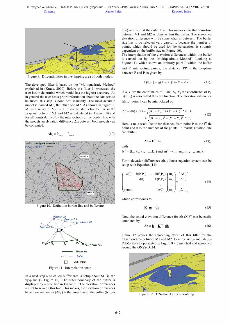
Figure 9. Discontinuities in overlapping area of both models

The developed filter is based on the “Multiquadratic Method” explained in (Kraus, 2000). Before the filter is processed the user has to determine which model has the highest accuracy. As in general the user has a priori information about the data sets to be fused, this step is done best manually. The most accurate model is named M1, the other one M2. As shown in Figure 8, M1 is a subset of M2. In a follow on step a border line in the xy-plane between M1 and M2 is calculated (s. Figure 10) and for all points defined by the intersections of the border line with the models an elevation difference Δhi between both models can be computed:

iZ(M2)iZ(M1)i PPΔh −= (10)

Figure 10. Definition border line and buffer are

Figure 11. Interpolation setup

In a next step a so called buffer area is setup about M1 in the xy-plane (s. Figure 10). The outer boundary of the buffer is displayed by a blue line in Figure 10. The elevation differences are set to zero on this line. This means, the elevation differences have their maximum (Δhi ) at the inner line of the buffer (border

line) and zero at the outer line. This makes clear that transition between M1 and M2 is done within the buffer. The smoothed elevation difference will be some what in between. The buffer size has to be selected very carefully, because the number of points, which should be used for the calculation, is strongly dependent on the buffer size (s. Figure 10). The interpolation of the elevation differences within the buffer is carried out by the “Multiquadratic Method”. Looking at Figure 11), which shows an arbitrary point P within the buffer and Pi intersecting points, the distance iPP in the xy-plane between P and Pi is given by 2

i2

ii )Y(Y)X(X)Pk(P, −+−= (11), if X,Y are the coordinates of P and Xi, Yi the coordinates of Pi.

)Pk(P, i is also called the core function. The elevation difference Δh for point P can be interpolated by

nm*)Y(Y)X(X

...m*)Y(Y)X(XY)h(X,h2

n2

n

12

12

1

−+−+

+−+−=Δ=Δ (12)

Here is mi a scale factor for distance from point P to the ith tie point and n is the number of tie points. In matrix notation one can write: mk T ⋅=Δh (13), with

)k...,,k,k,(k n321=Tk and )m...,,m,m,(m n321=Tm . For n elevation differences Δhi a linear equation system can be setup with Equation (13):

⎟⎟⎟⎟⎟

⎠

⎞

⎜⎜⎜⎜⎜

⎝

⎛

Δ

ΔΔ

=

⎟⎟⎟⎟⎟

⎠

⎞

⎜⎜⎜⎜⎜

⎝

⎛

⎟⎟⎟⎟⎟

⎠

⎞

⎜⎜⎜⎜⎜

⎝

⎛

n

2

1

n

2

1

n2

n121

h:hh

m:

mm

k(0)symm.:

)Pk(P...k(0))Pk(P...)Pk(Pk(0)

(14)

which corresponds to dhmK =⋅ (15) Now, the actual elevation difference for Δh (X,Y) can be easily computed by dhKk 1T ⋅⋅=Δ −h (16) Figure 12 proves the smoothing effect of this filter for the transition area between M1 and M2. Here the ALS- and GNSS-DTMs already presented in Figure 8 are matched and smoothed around the GNSS-DTM.

Figure 12. TIN-model after smoothing

In: Wagner W., Székely, B. (eds.): ISPRS TC VII Symposium – 100 Years ISPRS, Vienna, Austria, July 5–7, 2010, IAPRS, Vol. XXXVIII, Part 7BContents Author Index Keyword Index

642

4. CONCLUSIONS AND IMPROVEMENTS

The empirical test runs of the fusion algorithm show that good fusing results can be obtained. However, it performs best, if the models exhibit high elevation dynamic. In case of a plane the algorithm fails, because shifts in the horizontal are arbitrary. In this case the vertical shift can be determined by a special algorithm which first models the two planes and then determines the vertical shift between them. Operational test runs on real data show that if profile lines are regarded in ALS data modelling an improvement in the determination of excavated material in e.g. open mining is in the order of 0.1 m³/(m² surveyed area). In a further development step the algorithm will be extended so that also the three Euler orientations between the different data sets are determined. The smoothing algorithm proves its performance. All presented algorithms will be implemented in a commercial program.

5. REFERENCES

Kraus, K., 2000. Photogrammetrie, Band 3: Topographische Informationssysteme. 1. Aufl., Dümmler, Köln, pp. 137-145.

Ressl, C., Kager, H., Mandlburger, G., 2008. Quality checking of ALS projects using statistics of strip differences. In: The International Archives of the Photogrammetry, Remote Sensing and Spatial Information Sciences, Beijing, China, Vol. XXXVII, Part B3b, pp. 253-260.

Thiel, K.-H., Wehr, A., 2001. Operational production of DTMs using ScaLARS. In: Proceedings of OEEPE workshop on Airborne Laserscanning and Interferometric SAR for Detailed Digital Elevation Models, Stockholm, Sweden, paper 9.

Wehr, A., Petrescu, E., Duzelovic, H., Punz, Chr., 2009. Automatic break line detection out of high resolution airborne laser scanner data. In: Optical 3-D Measurement Techniques IX, Vienna, Austria, Vol. II, pp. 72-78.

In: Wagner W., Székely, B. (eds.): ISPRS TC VII Symposium – 100 Years ISPRS, Vienna, Austria, July 5–7, 2010, IAPRS, Vol. XXXVIII, Part 7BContents Author Index Keyword Index

643