Fusing Subcategory Probabilities for Texture Classification

Yang Song1, Weidong Cai1, Qing Li1, Fan Zhang1, David Dagan Feng1, Heng Huang2

1BMIT Research Group, School of IT, University of Sydney, Australia2Department of Computer Science and Engineering, University of Texas, Arlington, USA

Abstract

Texture, as a fundamental characteristic of objects, hasattracted much attention in computer vision research. Per-formance of texture classification is however still lacking forsome challenging cases, largely due to the high intra-classvariation and low inter-class distinction. To tackle these is-sues, in this paper, we propose a sub-categorization modelfor texture classification. By clustering each class into sub-categories, classification probabilities at the subcategory-level are computed based on between-subcategory distinc-tiveness and within-subcategory representativeness. Thesesubcategory probabilities are then fused based on their con-tribution levels and cluster qualities. This fused probabilityis added to the multiclass classification probability to ob-tain the final class label. Our method was applied to textureclassification on three challenging datasets – KTH-TIPS2,FMD and DTD, and has shown excellent performance incomparison with the state-of-the-art approaches.

1. IntroductionTexture provides important information for many com-

puter vision applications, such as material classification andscene and object recognition. Accurate classification of tex-ture images is however quite challenging. Some of the mainchallenges include the wide variety of natural texture pat-terns and large intra-class variation caused by illuminationand geometric changes, and relatively low inter-class dis-tinction [26, 41].

To tackle these challenges, extensive research has beenconducted to design highly discriminative and descriptivetexture features. Local texture descriptors have been thepredominant approaches with different ways of keypointselection, local descriptor design and histogram encod-ing [31, 25, 45, 29, 40, 37, 8]. Another research fo-cus is to incorporate feature invariance to key transfor-mations to accommodate the intra-class variations and en-hance the discriminative capability of texture descriptors[27, 41, 44, 9, 38, 35, 21, 34]. Classification at the finer

subcategory-level has also been explored [3, 8] by discov-ering subtypes in a texture category based on the concept ofvisual attributes [16, 2, 4, 24, 32].

On the other hand, the classification models used in tex-ture classification are usually quite standard. The most oftenused classifiers include the nearest neighbor (NN) approach[41, 44, 9, 40, 38], and support vector machine (SVM) withvarious kernel types [45, 29, 37, 35, 34, 8]. SVM is widelyrecognized as highly effective and usually boosts the dis-criminative power of feature descriptors compared to NN.However, it is a monolithic model and its performance canbe affected with large intra-class variations especially whenthere is considerable inter-class overlap in the feature space.

The sub-categorization method has recently been pro-posed to alleviate the problem of intra-class variations andinter-class ambiguity. It works by identifying the visualsubcategory structures of individual classes and modelingthe different subcategories independently. This could facil-itate better separation between different classes comparedto generating a monolithic model for the entire featurespace. The sub-categorization method generally containsthree main components: generation of subcategories, clas-sifier learning for individual subcategories, and fusion ofsubcategory results. Unsupervised clustering is usually per-formed for subcategory generation [46, 15, 1, 47]. Samplesfrom different classes are incorporated as additional con-straints to improve the clustering performance [12]. Fu-sion of subcategory results is typically performed by maxor mean pooling [46, 15, 1, 47], and second layer of classi-fier learning [19, 12]. The clustering step could also be dis-criminative and integrated with the classification objective[20]. Such methods have been shown to improve the classi-fication performance in various applications, including facerecognition [46], traffic sign categorization [15], object de-tection and recognition [19, 1, 47, 12], and discovering headorientations [20].

Different from the current studies in texture classifica-tion, which mostly focus on designing new texture featuredescriptors, our aim is to improve the classification accu-racy with a new classification model using existing features.

1

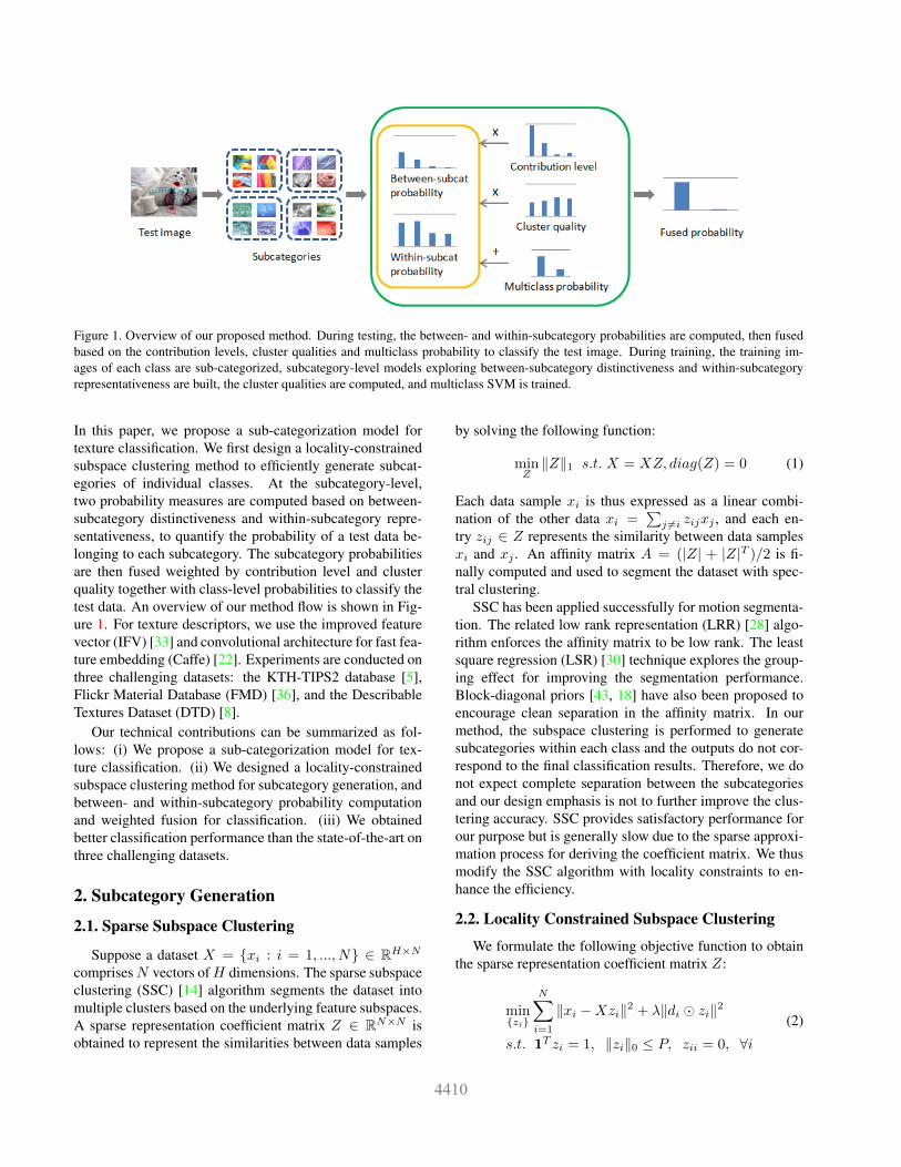
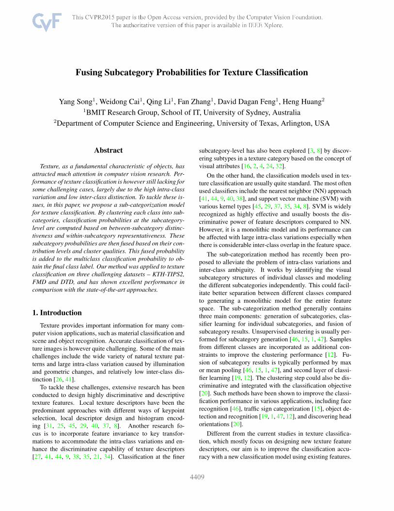
Figure 1. Overview of our proposed method. During testing, the between- and within-subcategory probabilities are computed, then fusedbased on the contribution levels, cluster qualities and multiclass probability to classify the test image. During training, the training im-ages of each class are sub-categorized, subcategory-level models exploring between-subcategory distinctiveness and within-subcategoryrepresentativeness are built, the cluster qualities are computed, and multiclass SVM is trained.

In this paper, we propose a sub-categorization model fortexture classification. We first design a locality-constrainedsubspace clustering method to efficiently generate subcat-egories of individual classes. At the subcategory-level,two probability measures are computed based on between-subcategory distinctiveness and within-subcategory repre-sentativeness, to quantify the probability of a test data be-longing to each subcategory. The subcategory probabilitiesare then fused weighted by contribution level and clusterquality together with class-level probabilities to classify thetest data. An overview of our method flow is shown in Fig-ure 1. For texture descriptors, we use the improved featurevector (IFV) [33] and convolutional architecture for fast fea-ture embedding (Caffe) [22]. Experiments are conducted onthree challenging datasets: the KTH-TIPS2 database [5],Flickr Material Database (FMD) [36], and the DescribableTextures Dataset (DTD) [8].

Our technical contributions can be summarized as fol-lows: (i) We propose a sub-categorization model for tex-ture classification. (ii) We designed a locality-constrainedsubspace clustering method for subcategory generation, andbetween- and within-subcategory probability computationand weighted fusion for classification. (iii) We obtainedbetter classification performance than the state-of-the-art onthree challenging datasets.

2. Subcategory Generation

2.1. Sparse Subspace Clustering

Suppose a dataset X = {xi : i = 1, ..., N} ∈ RH×N

comprisesN vectors ofH dimensions. The sparse subspaceclustering (SSC) [14] algorithm segments the dataset intomultiple clusters based on the underlying feature subspaces.A sparse representation coefficient matrix Z ∈ RN×N isobtained to represent the similarities between data samples

by solving the following function:

minZ‖Z‖1 s.t. X = XZ, diag(Z) = 0 (1)

Each data sample xi is thus expressed as a linear combi-nation of the other data xi =

∑j 6=i zijxj , and each en-

try zij ∈ Z represents the similarity between data samplesxi and xj . An affinity matrix A = (|Z| + |Z|T )/2 is fi-nally computed and used to segment the dataset with spec-tral clustering.

SSC has been applied successfully for motion segmenta-tion. The related low rank representation (LRR) [28] algo-rithm enforces the affinity matrix to be low rank. The leastsquare regression (LSR) [30] technique explores the group-ing effect for improving the segmentation performance.Block-diagonal priors [43, 18] have also been proposed toencourage clean separation in the affinity matrix. In ourmethod, the subspace clustering is performed to generatesubcategories within each class and the outputs do not cor-respond to the final classification results. Therefore, we donot expect complete separation between the subcategoriesand our design emphasis is not to further improve the clus-tering accuracy. SSC provides satisfactory performance forour purpose but is generally slow due to the sparse approxi-mation process for deriving the coefficient matrix. We thusmodify the SSC algorithm with locality constraints to en-hance the efficiency.

2.2. Locality Constrained Subspace Clustering

We formulate the following objective function to obtainthe sparse representation coefficient matrix Z:

min{zi}

N∑i=1

‖xi −Xzi‖2 + λ‖di � zi‖2

s.t. 1T zi = 1, ‖zi‖0 ≤ P, zii = 0, ∀i(2)

where zi ∈ RN is the ith column in Z indicating the sim-ilarity between xi and each sample in the dataset X . zi isP -sparse and Xzi is supposed to well approximate xi. Thesecond term, which is adopted from the locality-constrainedlinear coding (LLC) [42], encourages smaller coefficients tobe assigned to samples that are more different from xi withdi ∈ RN containing the pairwise Euclidean distances. Theconstant λ controls the balance between the two terms.

The coefficient vector zi can be efficiently obtained byfirst constructing a local codebook X̃i ∈ RH×P and dis-tance vector d̃i ∈ RP from P data samples in X that arethe most similar to xi (excluding xi). Then a P -dimensionalcoefficient vector z̃i is computed analytically via:

z̃∗i = (Vi + λdiag(d̃i)) \ 1z̃i = z̃∗i /(1

T z̃∗i )(3)

where Vi = (X̃i − xi1T )T (X̃i − xi1

T ). The coefficientvector zi is thus derived by mapping z̃i back to the N -dimensional space. Subsequently, similar to SSC, an affin-ity matrix is computed as A = (|Z|+ |Z|T )/2 and spectralclustering is performed to generate the clusters.

In our formulation, the dataset X contains the trainingdata of one class. The clustering outputs of X then corre-spond to the subcategories of that class. Each subcategorywould exhibit lower intra-class feature variation comparedto the entire class. Formally, we denote the dataset of oneclass c as Xc. Assume that Kc subcategories are gener-ated for Xc, which are denoted as {Sck : k = 1, ...,Kc}.These subcategories from all classes are then the bases forour probability estimation in the subsequent steps.

3. Subcategory Probabilities

We design two types of probability estimates at thesubcategory-level: the between-subcategory distinctivenessand within-subcategory representativeness. Both metricsmeasure the probabilities of a test data belonging to acertain subcategory. The difference is that the between-subcategory metric focuses on identifying the distinctionbetween subcategories of different classes while the within-subcategory metric captures the representativeness of thetest data by the particular subcategory.

3.1. Between-Subcategory Distinctiveness

The between-subcategory distinctiveness is obtainedbased on binary classification between a subcategory Sck

of class c and all subcategories {Sc′k′} of the other classes∀c′ 6= c and k′ = 1, ...,Kc′ . One binary classifier is trainedfor each subcategory using linear-kernel SVM. For a testdata x, a set of probability estimates {Pb(x, Sck) : ∀c, k} isthus derived to describe the probabilities of x belonging toeach subcategory using these trained binary classifiers [6].

3.2. Within-Subcategory Representativeness

The within-subcategory probability is derived based onthe representativeness of the test data by a subcategory.Different from the between-subcategory metric, the within-subcategory metric utilizes the training data of a certain sub-category Sck only and describes how well this subcategoryrepresents the test data x. A better representation corre-sponds to a higher probability of x belonging to Sck.

Specifically, given a test data x and a subcategory Sck,we first obtain an approximated x′ck by averaging the M -nearest neighbors of x from Sck. In this way, x is adaptedto the feature space of Sck. We choose the simple nearest-neighbor computation rather than the other encoding tech-niques such as the LLC, since we do not want x to be overlywell approximated by Sck and lose the subcategory-specificcharacteristics of the feature space. Next, assume the cen-ter of Sck is fck ∈ RH . The Euclidean distance betweenx′ck and fck then describes the representativeness of x bythe subcategory Sck. The probability of x belonging to thissubcategory is subsequently computed as:

Pw(x, Sck) = exp(−‖x′ck − fck‖) (4)

For the test data x, such within-subcategory probabilitiesare computed for all subcategories, and we obtain a set ofprobability estimates {Pw(x, Sck) : ∀c, k} at this step.

To derive the subcategory center fck, we adopt the sup-port vector data description (SVDD) [39] method with thefollowing objective:

minRck,fck

R2ck + C

Nck∑i=1

ξi

s.t. ‖x′ick − fck‖2 ≤ R2ck + ξi, ξi ≥ 0, ∀i

(5)

where Rck is a radius originating from the center fck, Nck

indicates the number of training data in Sck, x′ick denotesthe approximated xi ∈ Sck from the M -nearest neighborsin Sck (excluding xi), ξi is the slack variable and C is thetrade-off parameter. With this construct, Rck is expected tobe the smallest radius enclosing the data in Sck with slackvariables ξi to accommodate the outliers. The objectivefunction can be solved by introducing Lagrange multipli-ers αi as detailed in [39]. The data samples correspondingto nonzero αi form the support vectors, which are then lin-early combined as the center fck:

fck =∑i

αix′ick (6)

4. Subcategory Fusion

We finally fuse the subcategory-level probabilities to-gether with class-level classification probability to classify

the test data. The probability of test data x belonging toclass c is defined as:

P (x, c) = Pm(x, c) +

Kc∑k=1

wckqck{βPb(x, Sck)

+(1− β)Pw(x, Sck)}(7)

The first term Pm(x, c) is the probability of x belonging toclass c obtained using multiclass linear-kernel SVM, whichis trained without considering the subcategory structures.The second term is the class-level probability fused fromthe subcategory-level probabilities. The constant β controlsthe ratio between the two subcategory-level probabilities.The two weighting factors, wck and qck, represent the con-tribution level and cluster quality of subcategory Sck.

We suppose that higher contributions should come fromsubcategories that are more similar to x in the feature space.This level of similarity can be estimated by finding a sparserepresentation of x from the various subcategories. Specif-ically, we formulate the following function to obtain theweight vector w in a LLC construct:

minw‖x− Uw‖2 + λ‖d� w‖2

s.t. 1Tw = 1, ‖w‖0 ≤ P,(8)

The weight vector w of dimension J =∑

cKc is a con-catenation of factorswck from all subcategories. The matrixU ∈ RH×J contains the approximated x′ck from each sub-category Sck (Section 3.2), and Uw is expected to representx closely. The pairwise Euclidean distances between x andthe approximated vectors are stored in d to enforce the lo-cality constraints. The derived w is P -sparse and then usedas the weight factor in fusing the subcategory probabilities.

Our second design consideration is that subcategoriesrepresenting more compact and isolated clusters shouldcarry higher weights. The weight factor qck is computedto quantify such cluster quality based on the Dunn index(DI) [13]. DI measures the ratio between the minimal inter-cluster distance to maximal intra-cluster distance. In ourproblem, each subcategory is a cluster and one index qck iscomputed per subcategory by the following:

qck =mini,j ‖xi − xj‖maxi,i′ ‖xi − xi′‖

,

∀xi ∈ Sck, xi′ ∈ Sck, xj ∈ {Sc′k′}(9)

with c′ 6= c and k′ = 1, ...,Kc′ . The vector containing allweight factors is finally normalized to mean value of 1.

5. Experiments5.1. Datasets and Implementation

Three challenging texture datasets are used for our eval-uation, including the KTH-TIPS2 [5], FMD [36] and DTD

Table 1. Summary of the datasets used.Dataset Num. of images Num. of classes

KTH-TIPS2 4752 11FMD 1000 10DTD 5640 47

[8]. We choose these datasets since the state-of-the-art re-sults on them are all below 80% [8], while the performanceon the other popular datasets (e.g. UMD [44]) has becomerather saturated with over 99% accuracy. Table 1 summa-rizes the characteristics of the three datasets.

Two types of texture descriptors are applied to representthe images: the IFV [33] and Caffe [22] descriptors. Thecombination of IFV and deep convolutional network acti-vation features (DeCAF) [11] has shown excellent textureclassification accuracy in the state-of-the-art [8], achievingabout 9% improvement over the previous best result. In ad-dition, Caffe, being a more efficient and modularized frame-work, has recently been released to replace DeCAF. Sinceour focus is on the classification model rather than featuredesign, we choose to follow [8] and adopt IFV and Caffe asour feature descriptors.

IFV works by extracting local SIFT descriptors denselyat multiple scales, reducing the local feature dimensionusing principal component analysis (PCA), and encodingthem using a Gaussian mixture model (GMM) with mul-tiple modes. Signed square-rooting and L2 normalizationare also incorporated. The descriptor dimension is deter-mined by the reduced local feature length and the numberof modes with GMM. Similar to [8], SIFT descriptors arecomputed with a spatial extent of 6 × 6 pixels at scales2i/3, i = 0, ..., 4 and sampled every two pixels. The 128-dimensional SIFT descriptor is reduced to 64 dimensionsusing PCA. For KTH-TIPS2 and FMD datasets, 64 Gaus-sian modes are used; while for DTD, 256 modes are used.We try to use a small number of modes for KTH-TIPS2 andFMD in order to reduce the feature dimension. More modesare assigned for DTD compared to the other two datasetssince DTD contains a larger number of classes. The featureencoding toolbox [7] is adopted in our implementation.

Caffe features are computed using deep convolutionalneural network [23], which is trained from the ImageNetchallenge. The network involves several convolution, rec-tification, max pooling, and fully-connected layers. Simi-lar to [8], we remove the softmax and last fully-connectedlayer of the network to obtain a 4096-dimensional descrip-tor, which is then L2 normalized. The same approach isapplied to all three datasets.

The parameter settings in our sub-categorization classi-fication model are summarized as follows. For both sub-category generation and fusion, the sparsity constant P is

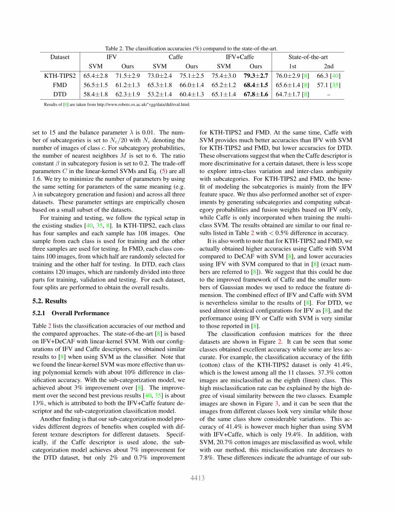
Table 2. The classification accuracies (%) compared to the state-of-the-art.Dataset IFV Caffe IFV+Caffe State-of-the-art

SVM Ours SVM Ours SVM Ours 1st 2ndKTH-TIPS2 65.4±2.8 71.5±2.9 73.0±2.4 75.1±2.5 75.4±3.0 79.3±2.7 76.0±2.9 [8] 66.3 [40]

FMD 56.5±1.5 61.2±1.3 65.3±1.8 66.0±1.4 65.2±1.2 68.4±1.5 65.6±1.4 [8] 57.1 [35]DTD 58.4±1.8 62.3±1.9 53.2±1.4 60.4±1.3 65.1±1.4 67.8±1.6 64.7±1.7 [8] –

Results of [8] are taken from http://www.robots.ox.ac.uk/˜vgg/data/dtd/eval.html.

set to 15 and the balance parameter λ is 0.01. The num-ber of subcategories is set to Nc/20 with Nc denoting thenumber of images of class c. For subcategory probabilities,the number of nearest neighbors M is set to 6. The ratioconstant β in subcategory fusion is set to 0.2. The trade-offparameters C in the linear-kernel SVMs and Eq. (5) are all1.6. We try to minimize the number of parameters by usingthe same setting for parameters of the same meaning (e.g.λ in subcategory generation and fusion) and across all threedatasets. These parameter settings are empirically chosenbased on a small subset of the datasets.

For training and testing, we follow the typical setup inthe existing studies [40, 35, 8]. In KTH-TIPS2, each classhas four samples and each sample has 108 images. Onesample from each class is used for training and the otherthree samples are used for testing. In FMD, each class con-tains 100 images, from which half are randomly selected fortraining and the other half for testing. In DTD, each classcontains 120 images, which are randomly divided into threeparts for training, validation and testing. For each dataset,four splits are performed to obtain the overall results.

5.2. Results

5.2.1 Overall Performance

Table 2 lists the classification accuracies of our method andthe compared approaches. The state-of-the-art [8] is basedon IFV+DeCAF with linear-kernel SVM. With our config-urations of IFV and Caffe descriptors, we obtained similarresults to [8] when using SVM as the classifier. Note thatwe found the linear-kernel SVM was more effective than us-ing polynomial kernels with about 10% difference in clas-sification accuracy. With the sub-categorization model, weachieved about 3% improvement over [8]. The improve-ment over the second best previous results [40, 35] is about13%, which is attributed to both the IFV+Caffe feature de-scriptor and the sub-categorization classification model.

Another finding is that our sub-categorization model pro-vides different degrees of benefits when coupled with dif-ferent texture descriptors for different datasets. Specif-ically, if the Caffe descriptor is used alone, the sub-categorization model achieves about 7% improvement forthe DTD dataset, but only 2% and 0.7% improvement

for KTH-TIPS2 and FMD. At the same time, Caffe withSVM provides much better accuracies than IFV with SVMfor KTH-TIPS2 and FMD, but lower accuracies for DTD.These observations suggest that when the Caffe descriptor ismore discriminative for a certain dataset, there is less scopeto explore intra-class variation and inter-class ambiguitywith subcategories. For KTH-TIPS2 and FMD, the bene-fit of modeling the subcategories is mainly from the IFVfeature space. We thus also performed another set of exper-iments by generating subcategories and computing subcat-egory probabilities and fusion weights based on IFV only,while Caffe is only incorporated when training the multi-class SVM. The results obtained are similar to our final re-sults listed in Table 2 with < 0.5% difference in accuracy.

It is also worth to note that for KTH-TIPS2 and FMD, weactually obtained higher accuracies using Caffe with SVMcompared to DeCAF with SVM [8], and lower accuraciesusing IFV with SVM compared to that in [8] (exact num-bers are referred to [8]). We suggest that this could be dueto the improved framework of Caffe and the smaller num-bers of Gaussian modes we used to reduce the feature di-mension. The combined effect of IFV and Caffe with SVMis nevertheless similar to the results of [8]. For DTD, weused almost identical configurations for IFV as [8], and theperformance using IFV or Caffe with SVM is very similarto those reported in [8].

The classification confusion matrices for the threedatasets are shown in Figure 2. It can be seen that someclasses obtained excellent accuracy while some are less ac-curate. For example, the classification accuracy of the fifth(cotton) class of the KTH-TIPS2 dataset is only 41.4%,which is the lowest among all the 11 classes. 37.3% cottonimages are misclassified as the eighth (linen) class. Thishigh misclassification rate can be explained by the high de-gree of visual similarity between the two classes. Exampleimages are shown in Figure 3, and it can be seen that theimages from different classes look very similar while thoseof the same class show considerable variations. This ac-curacy of 41.4% is however much higher than using SVMwith IFV+Caffe, which is only 19.4%. In addition, withSVM, 20.7% cotton images are misclassified as wool, whilewith our method, this misclassification rate decreases to7.8%. These differences indicate the advantage of our sub-

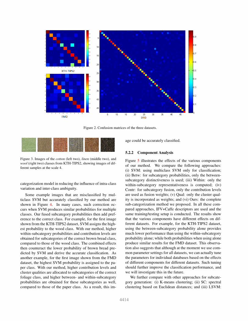
Figure 2. Confusion matrices of the three datasets.

Figure 3. Images of the cotton (left two), linen (middle two), andwool (right two) classes from KTH-TIPS2, showing images of dif-ferent samples at the scale 4.

categorization model in reducing the influence of intra-classvariation and inter-class ambiguity.

Some example images that are misclassified by mul-ticlass SVM but accurately classified by our method areshown in Figure 4. In many cases, such correction oc-curs when SVM produces similar probabilities for multipleclasses. Our fused subcategory probabilities then add pref-erence to the correct class. For example, for the first imageshown from the KTH-TIPS2 dataset, SVM assigns the high-est probability to the wood class. With our method, higherwithin-subcategory probabilities and contribution levels areobtained for subcategories of the correct brown bread class,compared to those of the wood class. The combined effectsthen counteract the lower probability of brown bread pre-dicted by SVM and derive the accurate classification. Asanother example, for the first image shown from the FMDdataset, the highest SVM probability is assigned to the pa-per class. With our method, higher contribution levels andcluster qualities are allocated to subcategories of the correctfoliage class, and higher between- and within-subcategoryprobabilities are obtained for these subcategories as well,compared to those of the paper class. As a result, this im-

age could be accurately classified.

5.2.2 Component Analysis

Figure 5 illustrates the effects of the various componentsof our method. We compare the following approaches:(i) SVM: using multiclass SVM only for classification;(ii) Betw: for subcategory probabilities, only the between-subcategory distinctiveness is used; (iii) Within: only thewithin-subcategory representativeness is computed; (iv)Contr: for subcategory fusion, only the contribution levelsare used as fusion weights; (v) Qual: only the cluster qual-ity is incorporated as weights; and (vi) Ours: the completesub-categorization method we proposed. In all these com-pared approaches, IFV+Caffe descriptors are used and thesame training/testing setup is conducted. The results showthat the various components have different effects on dif-ferent datasets. For example, for the KTH-TIPS2 dataset,using the between-subcategory probability alone providesmuch lower performance than using the within-subcategoryprobability alone; while both probabilities when using aloneproduce similar results for the FMD dataset. This observa-tion also suggests that although at the moment we use com-mon parameter settings for all datasets, we can actually tunethe parameters for individual databases based on the effectsof different components for different datasets. Such tuningshould further improve the classification performance, andwe will investigate this in the future.

We further compare with other approaches for subcate-gory generation: (i) K-means clustering; (ii) SC: spectralclustering based on Euclidean distances; and (iii) LSVM:

brown bread cotton cracker foliage glass leather cracked crosshatched dottedwood white bread brown bread paper plastic paper cobwebbed flecked perforated

lettuce leaf linen wool metal paper plastic fibrous grid groovedcotton cotton linen paper foliage paper interlaced chequered gauzy

(a) (b) (c)

Figure 4. Example images that are correctly classified by our proposed method but misclassified by SVM, from (a) KTH-TIPS2, (b) FMD,and (c) DTD. The tags on top of each image indicate the image label (upper) and the label predicted by SVM (lower).

Figure 5. Classification accuracies evaluating the various components of our proposed method.

using latent SVM to obtain the subcategories while itera-tively optimizing the classification objective [17, 10]. K-means and SC are used only to replace the subcategory gen-eration component of our method. LSVM is used to directlyobtain the classification results with the subcategories ini-tialized by our subcategory generation method. As shownin Figure 6, our subcategory generation method providesbetter classification results than K-means and SC. The onlydifference between our method and SC is the way of com-puting the affinity matrix, and the performance differenceindicates the advantage of our LLC-based sparse represen-tation formulation. The LSVM approach can be consid-ered as classifying based on the between-subcategory dis-tinctiveness only, even though the subcategory assignmentsare iteratively refined based on the classification outputs.The advantage of our method demonstrates the benefit ofintegrating the multiclass, between- and within-subcategoryprobabilities with weighted fusion. We also suggest thatbetter classification results using LSVM could possibly beobtained by improving the mining of training data, which ishowever not the focus of our current study.

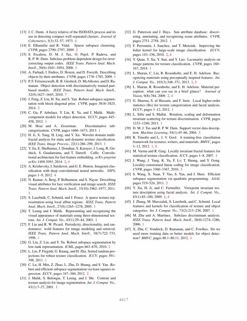
Figure 7 shows the visual results of our subcategorygeneration method. For each dataset, we choose a classthat we obtain large performance improvement over SVMto present the visual analysis. It can be seen that im-

ages of different subcategories tend to exhibit different tex-tures (e.g. periodicity, directionality and randomness) eventhough they belong to the same class. For example, imagesof the gauzy class in the DTD dataset can contain smoothor stripped surfaces, and the resultant subcategories cap-ture this difference in texture. Such differences can how-ever be harder to identify for the FMD dataset compared toKTH-TIPS2 and DTD, since the images in FMD are gen-erally more complex and the textures are often difficult todescribe or categorize. Nevertheless, our visual analysishelps to verify that our method can discover the subcate-gory structure in the data and is thus effective in enhancingthe texture classification performance by explicitly model-ing the subcategory-level classification.

6. Conclusions

In this paper, we have presented a sub-categorizationmodel for texture classification. The training images ofeach class are first clustered into subcategories with alocality-constrained subspace clustering method. We thendesign two subcategory-level probabilities to quantify theprobability of a test image belonging to each subcate-gory, with between-subcategory distinctiveness and within-subcategory representativeness. Finally, a weighted fusionmethod is designed to fuse the subcategory probabilities

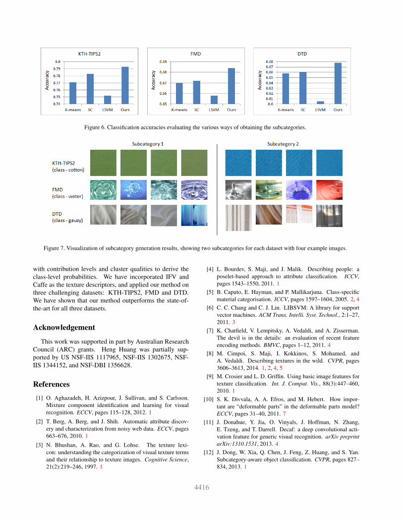
Figure 6. Classification accuracies evaluating the various ways of obtaining the subcategories.

Figure 7. Visualization of subcategory generation results, showing two subcategories for each dataset with four example images.

with contribution levels and cluster qualities to derive theclass-level probabilities. We have incorporated IFV andCaffe as the texture descriptors, and applied our method onthree challenging datasets: KTH-TIPS2, FMD and DTD.We have shown that our method outperforms the state-of-the-art for all three datasets.

Acknowledgement

This work was supported in part by Australian ResearchCouncil (ARC) grants. Heng Huang was partially sup-ported by US NSF-IIS 1117965, NSF-IIS 1302675, NSF-IIS 1344152, and NSF-DBI 1356628.

References

[1] O. Aghazadeh, H. Azizpour, J. Sullivan, and S. Carlsson.Mixture component identification and learning for visualrecognition. ECCV, pages 115–128, 2012. 1

[2] T. Berg, A. Berg, and J. Shih. Automatic attribute discov-ery and characterization from noisy web data. ECCV, pages663–676, 2010. 1

[3] N. Bhushan, A. Rao, and G. Lohse. The texture lexi-con: understanding the categorization of visual texture termsand their relationship to texture images. Cognitive Science,21(2):219–246, 1997. 1

[4] L. Bourdev, S. Maji, and J. Malik. Describing people: aposelet-based approach to attribute classification. ICCV,pages 1543–1550, 2011. 1

[5] B. Caputo, E. Hayman, and P. Mallikarjuna. Class-specificmaterial categorisation. ICCV, pages 1597–1604, 2005. 2, 4

[6] C. C. Chang and C. J. Lin. LIBSVM: A library for supportvector machines. ACM Trans. Intelli. Syst. Technol., 2:1–27,2011. 3

[7] K. Chatfield, V. Lempitsky, A. Vedaldi, and A. Zisserman.The devil is in the details: an evaluation of recent featureencoding methods. BMVC, pages 1–12, 2011. 4

[8] M. Cimpoi, S. Maji, I. Kokkinos, S. Mohamed, andA. Vedaldi. Describing textures in the wild. CVPR, pages3606–3613, 2014. 1, 2, 4, 5

[9] M. Crosier and L. D. Griffin. Using basic image features fortexture classification. Int. J. Comput. Vis., 88(3):447–460,2010. 1

[10] S. K. Divvala, A. A. Efros, and M. Hebert. How impor-tant are “deformable parts” in the deformable parts model?ECCV, pages 31–40, 2011. 7

[11] J. Donahue, Y. Jia, O. Vinyals, J. Hoffman, N. Zhang,E. Tzeng, and T. Darrell. Decaf: a deep convolutional acti-vation feature for generic visual recognition. arXiv preprintarXiv:1310.1531, 2013. 4

[12] J. Dong, W. Xia, Q. Chen, J. Feng, Z. Huang, and S. Yan.Subcategory-aware object classification. CVPR, pages 827–834, 2013. 1

[13] J. C. Dunn. A fuzzy relative of the ISODATA process and itsuse in detecting compact well-separated clusters. Journal ofCybernetics, 3(3):32–57, 1973. 4

[14] E. Elhamifar and R. Vidal. Sparse subspace clustering.CVPR, pages 2790–2797, 2009. 2

[15] S. Escalera, D. M. J. Tax, O. Pujol, P. Radeva, andR. P. W. Duin. Subclass problem-dependent design for error-correcting output codes. IEEE Trans. Pattern Anal. Mach.Intell., 30(6):1041–1054, 2008. 1

[16] A. Farhadi, I. Endres, D. Hoiem, and D. Forsyth. Describingobjects by their attributes. CVPR, pages 1778–1785, 2009. 1

[17] P. F. Felzenszwalb, R. B. Girshick, D. McAllester, and D. Ra-manan. Object detection with discriminatively trained part-based models. IEEE Trans. Pattern Anal. Mach. Intell.,32(9):1627–1645, 2010. 7

[18] J. Feng, Z. Lin, H. Xu, and S. Yan. Robust subspace segmen-tation with block-diagonal prior. CVPR, pages 3818–3825,2014. 2

[19] C. Gu, P. Arbelaez, Y. Lin, K. Yu, and J. Malik. Multi-component models for object detection. ECCV, pages 445–458, 2012. 1

[20] M. Hoai and A. Zisserman. Discriminative sub-categorization. CVPR, pages 1666–1673, 2013. 1

[21] H. Ji, X. Yang, H. Ling, and Y. Xu. Wavelet domain multi-fractal analysis for static and dynamic texture classification.IEEE Trans. Image Process., 22(1):286–299, 2013. 1

[22] Y. Jia, E. Shelhamer, J. Donahue, S. Karayev, J. Long, R. Gir-shick, S. Guadarrama, and T. Darrell. Caffe: Convolu-tional architecture for fast feature embedding. arXiv preprintarXiv:1408.5093, 2014. 2, 4

[23] A. Krizhevsky, I. Sutskever, and G. E. Hinton. Imagenet clas-sification with deep convolutional neural networks. NIPS,pages 1–9, 2012. 4

[24] N. Kumar, A. Berg, P. Belhumeur, and S. Nayar. Describingvisual attributes for face verification and image search. IEEETrans. Pattern Anal. Mach. Intell., 33(10):1962–1977, 2011.1

[25] S. Lazebnik, C. Schmid, and J. Ponce. A sparse texture rep-resentation using local affine regions. IEEE Trans. PatternAnal. Mach. Intell., 27(8):1265–1278, 2005. 1

[26] T. Leung and J. Malik. Representing and recognizing thevisual appearance of materials using three-dimensional tex-tons. Int. J. Comput. Vis., 43(1):29–44, 2001. 1

[27] F. Liu and R. W. Picard. Periodicity, directionality, and ran-domness: wold features for image modeling and retrieval.IEEE Trans. Pattern Anal. Mach. Intell., 18(7):722–733,1996. 1

[28] G. Liu, Z. Lin, and Y. Yu. Robust subspace segmentation bylow-rank representation. ICML, pages 663–670, 2010. 2

[29] L. Liu, P. Fieguth, G. Kuang, and H. Zha. Sorted random pro-jections for robust texture classification. ICCV, pages 391–398, 2011. 1

[30] C. Lu, H. Min, Z. Zhao, L. Zhu, D. Huang, and S. Yan. Ro-bust and efficient subspace segmentation via least squares re-gression. ECCV, pages 347–360, 2012. 2

[31] J. Malik, S. Belongie, T. Leung, and J. Shi. Contour andtexture analysis for image segmentation. Int. J. Comput. Vis.,43(1):7–27, 2001. 1

[32] G. Patterson and J. Hays. Sun attribute database: discov-ering, annotating, and recognizing scene attributes. CVPR,pages 2751–2758, 2012. 1

[33] F. Perronnin, J. Sanchez, and T. Mensink. Improving thefisher kernel for large-scale image classification. ECCV,pages 143–156, 2010. 2, 4

[34] Y. Quan, Y. Xu, Y. Sun, and Y. Luo. Lacunarity analysis onimage patterns for texture classification. CVPR, pages 160–167, 2014. 1

[35] L. Sharan, C. Liu, R. Rosenholtz, and E. H. Adelson. Rec-ognizing materials using perceptually inspired features. Int.J. Comput. Vis., 103(3):348–371, 2013. 1, 5

[36] L. Sharan, R. Rosenholtz, and E. H. Adelson. Material per-ception: what can you see in a brief glance? Journal ofVision, 9(8):784, 2009. 2, 4

[37] G. Sharma, S. ul Hussain, and F. Jurie. Local higher-orderstatistics (lhs) for texture categorization and facial analysis.ECCV, pages 1–12, 2012. 1

[38] L. Sifre and S. Mallat. Rotation, scaling and deformationinvariant scattering for texture discrimination. CVPR, pages1233–1240, 2013. 1

[39] D. M. J. Tax and R. P. W. Duin. Support vector data descrip-tion. Machine Learning, 54(1):45–66, 2004. 3

[40] R. Timofte and L. J. V. Gool. A training-free classifiationframework for textures, writers, and materials. BMVC, pages1–12, 2012. 1, 5

[41] M. Varma and R. Garg. Locally invariant fractal features forstatistical texture classification. ICCV, pages 1–8, 2007. 1

[42] J. Wang, J. Yang, K. Yu, F. Lv, T. Huang, and Y. Gong.Locality-constrained linear coding for image classification.CVPR, pages 3360–3367, 2010. 3

[43] S. Wang, X. Yuan, T. Yao, S. Yan, and J. Shen. Efficientsubspace segmentation via quadratic programming. AAAI,pages 519–524, 2011. 2

[44] Y. Xu, H. Ji, and C. Fermuller. Viewpoint invariant tex-ture description using factal analysis. Int. J. Comput. Vis.,83(1):85–100, 2009. 1, 4

[45] J. Zhang, M. Marszalek, S. Lazebnik, and C. Schmid. Localfeatures and kernels for classification of texture and objectcategories. Int. J. Comput. Vis., 73(2):213–238, 2007. 1

[46] M. Zhu and A. Martinez. Subclass discriminant analysis.IEEE Trans. Pattern Anal. Mach. Intell., 28(8):1274–1286,2006. 1

[47] X. Zhu, C. Vondrick, D. Ramanan, and C. Fowlkes. Do weneed more training data or better models for object detec-tion? BMVC, pages 80.1–80.11, 2012. 1