Embed Size (px)
Citation preview
7/28/2019 Fulltext01 Chapter 4
http://slidepdf.com/reader/full/fulltext01-chapter-4 1/80
Quality Inspection and FatigueAssessment of Welded Structures In Cooperation WithVolvo Construction Equipment AB
ERIC LINDGRENTHOMAS STENBERG
Master of Science Thesis in Lightweight StructuresDept of Aeronautical and Vehicle Engineering
Stockholm, Sweden 2011
7/28/2019 Fulltext01 Chapter 4
http://slidepdf.com/reader/full/fulltext01-chapter-4 2/80
QUALITY INSPECTION AND FATIGUE ASSESSMENT OF WELDED
STRUCTURES
Eric LindgrenThomas Stenberg
Master of Science Thesis TRITA AVE 2011:02 ISSN 1651-7660
KTH Industrial Engineering and Management
Lightweight Structures
SE-100 44 STOCKHOLM
7/28/2019 Fulltext01 Chapter 4
http://slidepdf.com/reader/full/fulltext01-chapter-4 3/80
1
Master of Science Thesis TRITA AVE 2011:02 ISSN 1651-7660
Quality Inspection and Fatigue Assessment
of Welded Structures
Eric Lindgren
Thomas Stenberg
Approved
2011-03-10
Examiner
Stefan Hallström
Supervisor
Zuheir Barsoum
Commissioner
Volvo Construction Equipment AB
Contact person
Bertil Jonsson
Abstract
Recently, Volvo Construction Equipment AB has developed a weld class system for imperfections in welded joints, which contains demands for the toe radii, cold laps, undercutsetc. and where root defects are treated as requirements on the drawing. In this master thesis, thetoe radius has been studied more carefully along with the selection of reliable measurementsystems which are able to measure the toe radius along the weld. A computerized vision systemhas been evaluated by performing a measurement system analysis. FE-simulations anddestructive fatigue testing has also been carried out to determine which radial geometry beingcritical to the fatigue life.
The results show that the currently used methods and gauges do not provide the requiredaccuracy when measuring the toe radius. The gauges are handled differently by differentoperators – even when using the vision system – which makes the methods subjective andtherefore unreliable. There are measuring systems that can gather surface data along the weldwith high accuracy, but there is no reliable method to assess the data. Therefore, the authors havedeveloped an algorithm – named STELIN – that assess the gathered surface data andautomatically identifies and calculates the toe radius and the toe angle along the weld. Using thatinformation an opportunity to improve the process control when welding is possible.
The performed FE-calculations show that the surface roughness in the weld toe probably has aninfluence at the fatigue life of the joint. A more precise separate study should be made todetermine the impact of the surface roughness on the fatigue life. Those results should serve as a
base when reviewing the theory used when predicting the fatigue life. Currently, stress averagingapproach is used in the notches of the root and the weld toe. In the future though, there might beanother stress condition to be taken into account, if the goal of reducing weight of the finished
product shall be achieved. Regarding measuring the surface roughness in the weld toe, theevaluated vision system has enough accuracy to deliver reliable data.
More work remains with the STELIN-algorithm. The method used when assessing the calculatedtoe radii should be based on the conclusions from the performed FE-calculations. Integrating theSTELIN-algorithm in a fast feedback measurement system – for instance, on a laser – will
probably provide good opportunities for a better process control in order to achieve higher fatigue life of the welded joint.

7/28/2019 Fulltext01 Chapter 4
http://slidepdf.com/reader/full/fulltext01-chapter-4 4/80
2
FOREWORD
First we would like to thank our supervisors:
Zuheir Barsoum, PhD, Sr Lecturer, KTH – Lightweight Structures.
Bertil Jonsson, Expert Weld Strength, Volvo Construction Equipment AB.for their commitment and encouraging support during our work with this master thesis.
For their providing with acknowledge help, feedback and inspiration when developing thealgorithm, we would like to thank:
Lennart Edsberg, Associate Professor, KTH – Computer Science and Communication atthe department of Scientific Computing.
Arne Leijon, Professor, KTH – School of Electrical Engineering at the department of Sound and Image Processing.
We would also like to thank Joakim Hedegård, Jukka-Pekka Anttonen and Pontus Rydgren atSwerea KIMAB AB – Centre for Joining & Structures, by providing measurement equipmentand reading through the manuscript.
Eric Lindgren Thomas Stenberg070 – 632 26 08 073 – 028 91 [email protected] [email protected]
Stockholm March 10, 2011
7/28/2019 Fulltext01 Chapter 4
http://slidepdf.com/reader/full/fulltext01-chapter-4 5/80
3
NOMENCLATURE
Here are the abbreviations that are used in this master thesis.
Abbreviat ions
WIQ Weight reduction by Improved weld Quality
VCE Volvo Construction Equipment AB
WPS Welding Procedure Specification
GMAW Gas Metal Arc Welding
MIG Metal Inert Gas MAG Metal Active Gas
FCAW Flux Cored Arc Welding
TIG Tungsten Inert Gas
EDM Electric Discharge Machining
FEM Finite Element Method
FE Finite Element
ESM Effective notch Stress Method
CET Cutting Edge Tool
SLP Stripe Light Projection
MSA Measurement System Analysis… …
7/28/2019 Fulltext01 Chapter 4
http://slidepdf.com/reader/full/fulltext01-chapter-4 6/80
4
TABLE OF CONTENTS
1 INTRODUCTION ............................................................................................................. 5
1.1 Background ....................................................................................................... 5
1.2 Purpose ............................................................................................................. 5
1.3 Delimitations .................................................................................................... 5
1.4 Method .............................................................................................................. 6
2 TEST SPECIMENS .......................................................................................................... 7
2.1 MIG/MAG welding .......................................................................................... 8
2.2 Shot peening ..................................................................................................... 9
2.3 TIG-dressing ................................................................................................... 10
2.4 Dimensional requirements .............................................................................. 11
2.5 Quality inspection ........................................................................................... 13
3 GAUGES .......................................................................................................................... 14
3.1 Currently used gauges .................................................................................... 14
3.2 The MikroCAD 26x20.................................................................................... 15
3.3 The Olympus LEXT OLS3000....................................................................... 19
3.4 The basics of a measurement system analysis ................................................ 20 3.5 Measuring operation ....................................................................................... 21
3.6 Results from test measuring ........................................................................... 21
3.7 Radial requirements according to STD 181-0004 .......................................... 22
3.8 Conclusions .................................................................................................... 23
4 STELIN ALGORITHM: EVALUATE THE GEOMETRY ....................................... 24
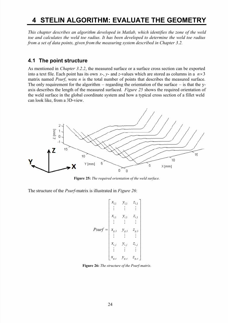
4.1 The point structure .......................................................................................... 24
4.2 Flow chart of the algorithm ............................................................................ 25
4.3 Calculating the radius of a circle .................................................................... 25
4.4 Describing the weld geometry as a curvature ................................................. 27
4.5 Using a filter ................................................................................................... 32
4.6 Identifying the boundaries for the weld toe .................................................... 33 4.7 Evaluating the obtained data........................................................................... 34
4.8 Extra features of the algorithm ....................................................................... 35
4.9 Results when running the algorithm ............................................................... 37
5 FATIGUE ASSESSMENT ............................................................................................. 42
5.1 Location of surface inhomogeneity ................................................................ 44
5.2 Size of surface inhomogeneity ....................................................................... 49
6 DESTRUCTIVE TESTING ........................................................................................... 52
6.1 Fatigue test results .......................................................................................... 52
7 DISCUSSION AND CONCLUSIONS .......................................................................... 57
7.1 Discussion ....................................................................................................... 57
7.2 Conclusions .................................................................................................... 58 8 RECOMMENDATIONS AND FUTURE WORK ....................................................... 59
8.1 Recommendations .......................................................................................... 59
8.2 Future work..................................................................................................... 59
9 REFERENCES ................................................................................................................ 60
APPENDIX A: DRAWINGS...................................................................................................... 62
APPENDIX B: WELDING PARAMETERS ........................................................................... 64
APPENDIX C: WPS ................................................................................................................... 65
APPENDIX D: SILICONE CASTING ..................................................................................... 68
APPENDIX E: MEASUREMENT INSTRUCTION ............................................................... 70
APPENDIX F: ELEMENT SIZE .............................................................................................. 77

7/28/2019 Fulltext01 Chapter 4
http://slidepdf.com/reader/full/fulltext01-chapter-4 7/80
5
1 INTRODUCTION
This chapter describes the background, the purpose, the delimitations and the methods used in
this master thesis.
1.1 BackgroundDesirable goals when developing new construction equipment – wheel loaders, articulatedhaulers etc. – are to obtain improved performance, low fuel consumption, increased enduranceand lower production cost. In order to continuously improve the ability to produce lightweighthigh-performance equipment, an extensive research project named WIQ is running in both
production and development at VCE. A new weld class system has been developed at VCE,which follows the principle of “design for purpose” by employing a good relation between
acceptance limits and fatigue strength. Although, specifying the quality of a weld also requiresreliable methods to inspect and evaluate the process outcome. Thus, the choice of gauge andevaluation method is important in order to achieve reliable results.
1.2 Purpose
In the new Volvo Group weld class system STD 181-0004 there is a requirement which statesthe minimum weld toe radius. In this thesis, the weld toe radius shall be measured with a visionsystem provided by Toponova AB. The measurements will be performed on test specimens of awelded cruciform joint.
The performance factors of the vision system such as distribution and accuracy will be measuredand evaluated by using the measurement system analysis method. The intention is to use thevision system as an integrated inspection tool in the quality system.
Fatigue testing will be performed on non-load carrying welded joints in order to study:
The distribution in fatigue life. The crack initiation point in the weld and compare it with the measurements of the weld
geometry to determine the relationship between the toe radius and the crack initiation point.
FE-simulation shall be made to determine: The welded joints fatigue strength due to a varied toe radius.
What is to be considered as a dangerous – low fatigue life – weld toe radius if the surfacegeometry is complex.
1.3 Delimitations
Only the surface geometry of a non-load carrying cruciform joint will be evaluated. Only the toe radius in the surface will be evaluated. 2D-modells will be used when performing the simulation of the structure. The measurement system analysis will only be performed on the vision system provided
by Toponova AB.

7/28/2019 Fulltext01 Chapter 4
http://slidepdf.com/reader/full/fulltext01-chapter-4 8/80
6
1.4 Method
A literary study shall be performed to provide more background information about:
Measurement system analysis and how do determine the precision and accuracy. WPS, material and what to be considered during welding. How to determine a radius based on a set of data points. Fatigue life assessment.
A parametric FE-model of the test specimens shall be built in order to simulate fatigue testing in ANSYS Classic[1].
Establish a WPS and weld the test specimens, then measure the weld geometry with themeasurement system provided by Toponova AB.
Find a few different ways to measure and evaluate the weld toe radius in the surface profilemeasured by the vision system.
Perform fatigue life testing on the measured test specimens, evaluate the distribution anddetermine an average fatigue life.
7/28/2019 Fulltext01 Chapter 4
http://slidepdf.com/reader/full/fulltext01-chapter-4 9/80
7
2 TEST SPECIMENS
This chapter contains information about the test specimens. For example welding parameters,
used post-treatments, dimension requirements etc.
The test specimens to be studied are non-load carrying cruciform joints. These are manufactured
from steel (S355MC according to SS-EN 10149-2[1]) with a plates thickness of 10 mm and withthe weld filler material (Elga 100 MXA). Five different panels are produced in order to evaluatethe fatigue life depending on the post-treatment method. Two of the panels will not receive any
post-treatment, two panels will be shot peened and one panel will be TIG-dressed on the criticalweld toe. The shot peening is performed after cutting the panels in order to ensure that thecompressive stresses in the surface from the peening is not relaxed.
The panels are cut into 20 specimens according to APPENDIX A: DRAWINGS . Before thewelding operation, the panels have to be oriented so they match the drawings. Since there is nostandardized fixture available, the orientation is performed manually by using a measuring tape.Short tack welds with a length of 5 mm are used to fix the panels before the tack weld of 60 mmare performed. The location of the tack weld is marked on the flange of each panel with redcolor. When the full length welding of the panels are performed, the recommended welding
parameters in APPENDIX B: WELDING PARAMETERS are used with the procedure accordingto APPENDIX C: WPS . The WPS document contains essential information about the welding
procedure to be performed according to SS-EN ISO 15609-1:2004[3].
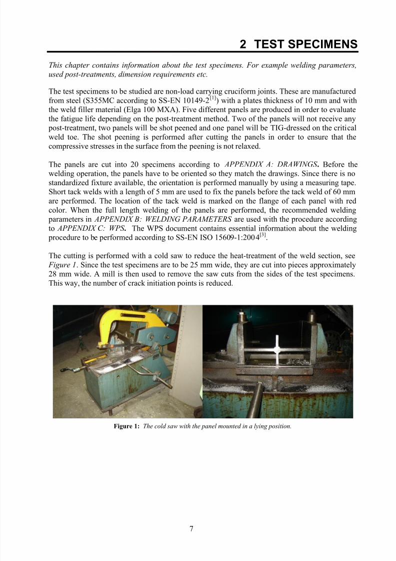
The cutting is performed with a cold saw to reduce the heat-treatment of the weld section, see Figure 1. Since the test specimens are to be 25 mm wide, they are cut into pieces approximately28 mm wide. A mill is then used to remove the saw cuts from the sides of the test specimens.This way, the number of crack initiation points is reduced.
Figure 1: The cold saw with the panel mounted in a lying position.

7/28/2019 Fulltext01 Chapter 4
http://slidepdf.com/reader/full/fulltext01-chapter-4 10/80
8
After the cutting operation, an individual identification number is engraved on the test specimen,see Figure 2. The identification number is written as X-Y, were X is the panel number and Y isthe rod number. It is important that the identification number is engraved on the flange. Thus, thenumbers of crack initiation points are reduced.
Figure 2: The marking spot on the test specimen and weld sequence.
2.1 MIG/MAG welding
This has been the manufacturing industries most popular welding method for several decadesnow. The method is a fuse welding application, where an electric arc melts a continuously fedelectrode in a shield gas. Because of the fed electrode the process is semi-automatic and theapplication is well designed for mechanization in an anthropomorphic robot, see Figure 3. Thetwo different types of GMAW have separate purposes, MIG welding are using an inert shieldinggas which does not react with the melted metal. MAG welding uses an active gas that reacts withthe melted metal according to Weman[4]. The GMAW parameters are grouped in two categories,
first the changeable welding input parameters and second, the recordable welding output parameter when the arc is running.
Input parameters: Electrode diameter Protruding wire length Voltage Weaving frequency Weaving amplitude Gas flow
Welding speed Wire feed
Output parameter: Current
MAG welding is commonly used for non- and low-alloyed steels. The MIG welding is used for high-, magnesium-, titan-, copper- and nickel-alloyed steels. Common scope for plate thicknessis 1 – 25 mm.
Figure 3: Robotic welding of the panels.
7/28/2019 Fulltext01 Chapter 4
http://slidepdf.com/reader/full/fulltext01-chapter-4 11/80
9
2.2 Shot peening
Shot peening is mainly used after welding but before painting to ensure a successful paintingoperation. However, shot peening can also be regarded as a post-treatment method, which willincrease the fatigue life on metal structures with dynamic loads. The method consists of shootingsmall round particles of steel, glass or ceramic compounds on the structures surface. Thus, thesurface is exposed for a plastic deformation. When performing this type of post-treatments, thegoal is to induce compressive stresses into the metals surface. The compressive stresses in thesurface are increasing the crack initiation threshold value for the structure. This is more desirablefrom a fatigue point of view since tensile stresses results in higher crack propagation. Thus,defects at the surface are permanently closed until the stresses have disappeared by the relaxationToday, it is normal to use automatic machines to control the process parameters:
The size and shape of particles – it should not exceed half the radius and a ¼ of thesmallest hole in the component that is being shot peened.
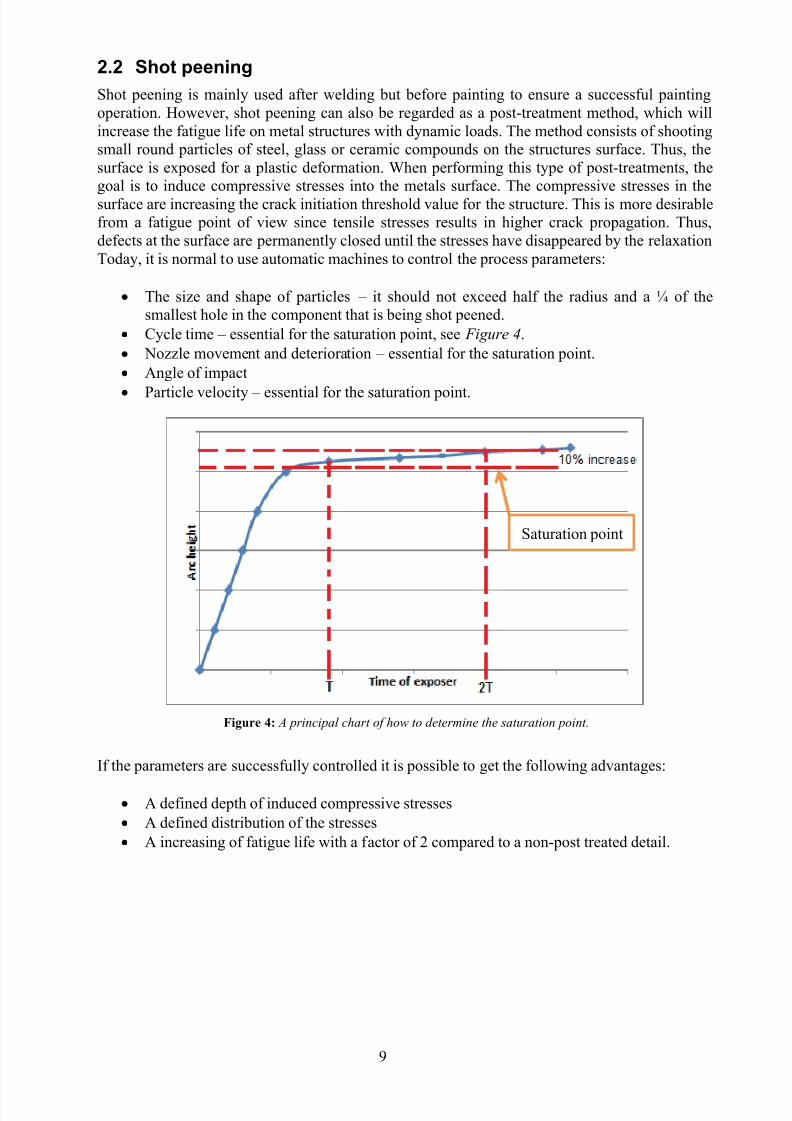
Cycle time – essential for the saturation point, see Figure 4. Nozzle movement and deterioration – essential for the saturation point. Angle of impact
Particle velocity – essential for the saturation point.
Figure 4: A principal chart of how to determine the saturation point.
If the parameters are successfully controlled it is possible to get the following advantages:
A defined depth of induced compressive stresses A defined distribution of the stresses A increasing of fatigue life with a factor of 2 compared to a non-post treated detail.
Saturation point
7/28/2019 Fulltext01 Chapter 4
http://slidepdf.com/reader/full/fulltext01-chapter-4 12/80
10
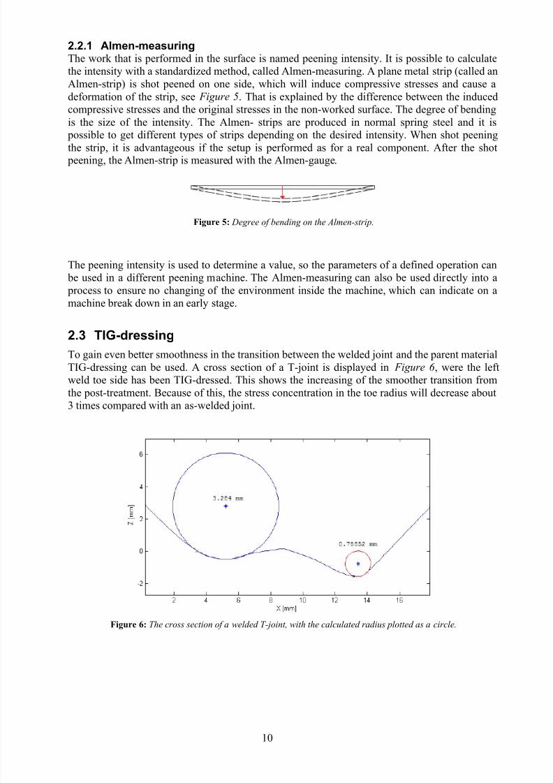
2.2.1 Almen-measuringThe work that is performed in the surface is named peening intensity. It is possible to calculatethe intensity with a standardized method, called Almen-measuring. A plane metal strip (called anAlmen-strip) is shot peened on one side, which will induce compressive stresses and cause adeformation of the strip, see Figure 5. That is explained by the difference between the inducedcompressive stresses and the original stresses in the non-worked surface. The degree of bendingis the size of the intensity. The Almen- strips are produced in normal spring steel and it is
possible to get different types of strips depending on the desired intensity. When shot peeningthe strip, it is advantageous if the setup is performed as for a real component. After the shot peening, the Almen-strip is measured with the Almen-gauge.
Figure 5: Degree of bending on the Almen-strip.
The peening intensity is used to determine a value, so the parameters of a defined operation can
be used in a different peening machine. The Almen-measuring can also be used directly into a process to ensure no changing of the environment inside the machine, which can indicate on amachine break down in an early stage.
2.3 TIG-dressing
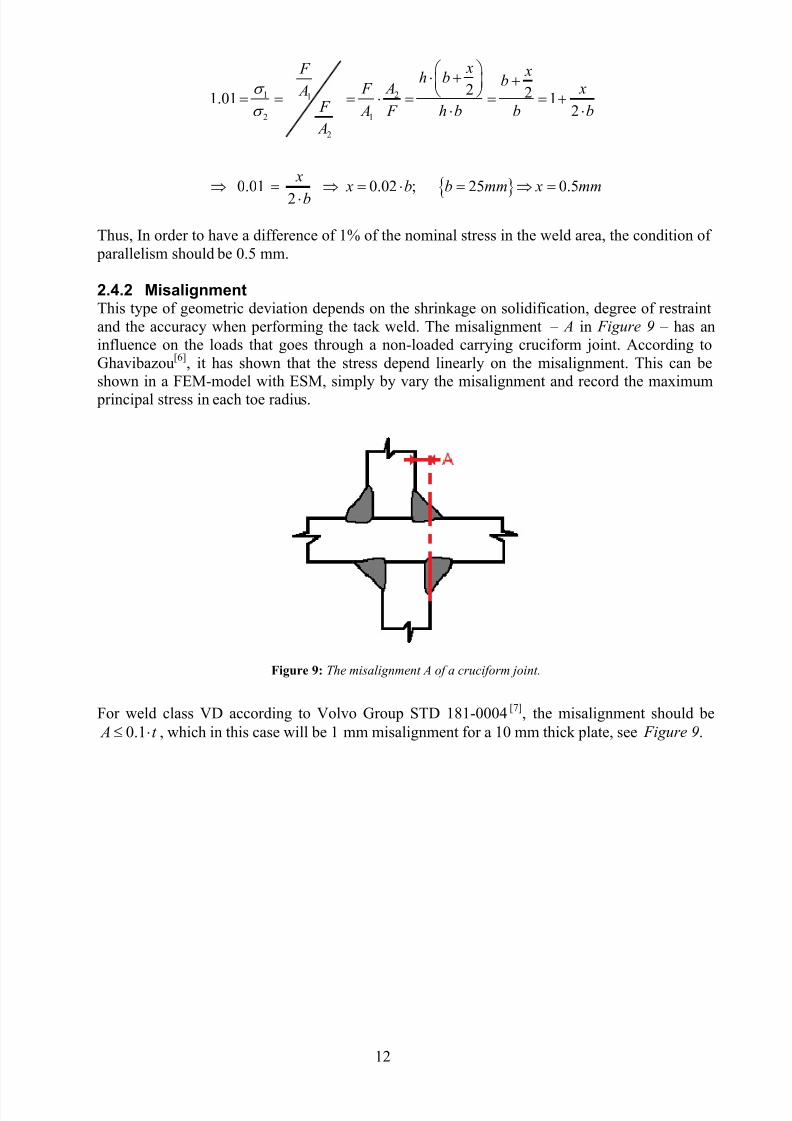
To gain even better smoothness in the transition between the welded joint and the parent materialTIG-dressing can be used. A cross section of a T-joint is displayed in Figure 6 , were the leftweld toe side has been TIG-dressed. This shows the increasing of the smoother transition fromthe post-treatment. Because of this, the stress concentration in the toe radius will decrease about3 times compared with an as-welded joint.
Figure 6: The cross section of a welded T-joint, with the calculated radius plotted as a circle.

7/28/2019 Fulltext01 Chapter 4
http://slidepdf.com/reader/full/fulltext01-chapter-4 13/80
11
The process is re-melting the transition line and moves it further up on the parent metal. Thiswill also decrease the level of inner defects (slag, etc.) and fuses cold laps according to
Narström[5]. The TIG-dressing can be performed with the ordinary TIG-equipment, but one of the cons is the low travel speed (around 50 – 200 mm/min). Therefore, this method only is usedon special selected areas on the component.
The parameters used when TIG-dressing the panels are shown in APPENDIX B: WELDING
PARAMETERS .
2.4 Dimensional requirements
To minimize the influence from the manufacturing some dimension requirements of the testspecimens are necessary. These requirements are listed below:
Parallelism – To assure the same nominal stress in the test specimen. Misalignment – To assure the same stress concentration in all toe radii. Perpendicular alignment – To easier assure a correct weld throat.
2.4.1 ParallelismWhen performing a fatigue life testing, it is important that the test specimens have the samedimensions. A cutting operation performed by a saw requires parallelism of the sides on the testspecimens. Therefore, a minimum requirement of the parallelism after cutting needs to bedecided. One way to do this is to evaluate the nominal stress in the weld area for two differentcross sections; parallel and non-parallel, see Figure 7 and Figure 8.
Figure 7: Parallel cross section. Figure 8: Non-parallel cross section.
Assume that the two different cross sections are loaded with a force F and F A , the
different areas for the cross sections will be:
1 1
1
2 2
22
2
F F A h b A h b
x F F A h b
x Ah b
A suitable condition for the parallelism should be that the difference in the cross section areashould not affect the nominal stress more than 1%. By comparing the stresses 1
and 2 , the
quote should be 1.01 if 1% difference is requested.
7/28/2019 Fulltext01 Chapter 4
http://slidepdf.com/reader/full/fulltext01-chapter-4 14/80
12
1 21
2 1
2
2 21.01 12
0.01 0.02 ; 25 0.52
x F xh b b A F x A
F A F h b b b A
x x b b mm x mm
b
Thus, In order to have a difference of 1% of the nominal stress in the weld area, the condition of parallelism should be 0.5 mm.
2.4.2 MisalignmentThis type of geometric deviation depends on the shrinkage on solidification, degree of restraintand the accuracy when performing the tack weld. The misalignment – A in Figure 9 – has aninfluence on the loads that goes through a non-loaded carrying cruciform joint. According toGhavibazou[6], it has shown that the stress depend linearly on the misalignment. This can beshown in a FEM-model with ESM, simply by vary the misalignment and record the maximum
principal stress in each toe radius.
Figure 9: The misalignment A of a cruciform joint.
For weld class VD according to Volvo Group STD 181-0004[7], the misalignment should be0.1 A t , which in this case will be 1 mm misalignment for a 10 mm thick plate, see Figure 9.
7/28/2019 Fulltext01 Chapter 4
http://slidepdf.com/reader/full/fulltext01-chapter-4 15/80
13
2.5 Quality inspection
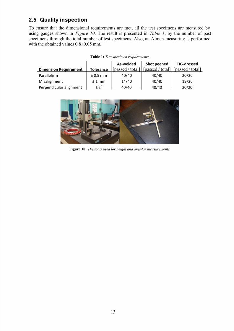
To ensure that the dimensional requirements are met, all the test specimens are measured byusing gauges shown in Figure 10. The result is presented in Table 1, by the number of pastspecimens through the total number of test specimens. Also, an Almen-measuring is performedwith the obtained values 0.8±0.05 mm.
Table 1: Test specimen requirements.
Dimension Requirement Tolerance
As-welded
[passed / total]Shot peened
[passed / total]
TIG-dressed
[passed / total]
Parallelism ± 0,5 mm 40/40 40/40 20/20
Misalignment ± 1 mm 14/40 40/40 19/20
Perpendicular alignment ± 2⁰ 40/40 40/40 20/20
Figure 10: The tools used for height and angular measurements.

7/28/2019 Fulltext01 Chapter 4
http://slidepdf.com/reader/full/fulltext01-chapter-4 16/80
14
3 GAUGES
This chapter gives a short description of the currently used gauges at VCE for measuring the
weld toe radius. Also, the vision system is briefly described, along with the process of performing
a measurement system analysis with its goals and outcome.
3.1 Currently used gauges
Currently, two different gauges are used at VCE to measure the weld toe radius; the first is areference block – see Figure 11 – and the other is a feeler gauge, see Figure 12.
3.1.1 The reference blockThe reference block is manufactured from a solid block by using wire EDM to gain high
precision of the surface and geometry (± 0.03 mm according to the manufacturer). The block issupposed to resemble a welded cruciform joint. The difference between the four sides is that theweld toe radius is of different sizes; that is 4 mm, 1 mm, 0.25 mm and ≈0 mm. The side of ≈ 0mm was intended to be as sharp as possible, aiming to define a radius that is nearly 0 mm. The
philosophy is to symbolize the three different weld classes in the Volvo Group STD 181-0004, to
perform a subjective evaluation of the toe radius in the weldment.
Figure 11: The reference block.
The measuring operation is performed manually by visually looking at the weld toe of the testspecimen. Then, by using the reference block as a reference, the operator determines the weldtoe radius with an estimation based on the visual difference between the test specimen and thereference block. The results are strongly influenced by the operators judgment, since differentoperators estimates the radius differently.
3.1.2 The feeler gaugeThe feeler gauge contains a set of blades were the end of every blade has a predefined radius, see
Figure 13. The measuring operation is performed manually, were the operator tries different blades – with different radius – and determines which blade that has the best fit against the testspecimens weld toe.
Figure 12: The feeler gauge.

7/28/2019 Fulltext01 Chapter 4
http://slidepdf.com/reader/full/fulltext01-chapter-4 17/80
15
The best fit is determined visually by the operator. Again, this method is strongly influenced bythe judgment of the operator, since it is up to the operator to decide if it is a good fit of the feeler gauge or not.
Figure 13: A principal draft of a blade on the feele gauge with the radius r .
3.2 The MikroCAD 26x20
An alternative method to measure the weld toe radius is to scan the weldment surface and perform the measuring in a computer environment. One of the goals with this thesis is toevaluate a computerized vision system provided by Toponova AB[8].
This system is a vision-system, which is developed by GFM[9] in Germany, the model of thesystem is MikroCAD 26x20[10], see Figure 14. Specifications about the measurement system are
presented in Table 2.
Figure 14: The MikroCAD 26x20 system.
Table 2: The specification of the MikroCAD 26x20 system.
Measuring volume 26 x 20 x 6 mm³
Number of meas. Points 1600 x 1200
Measuring time 2- 8 s
Lateral Resolution 15 µm
Vertical Resolution 2 µm
7/28/2019 Fulltext01 Chapter 4
http://slidepdf.com/reader/full/fulltext01-chapter-4 18/80
16
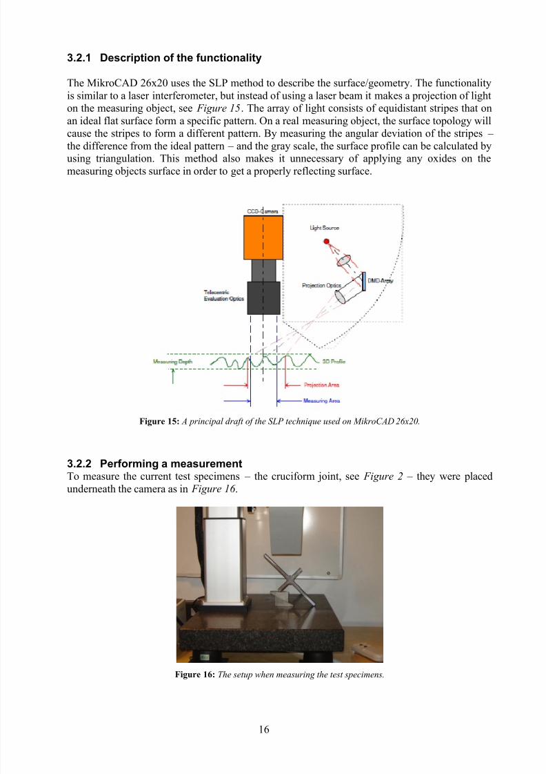
3.2.1 Description of the functionality
The MikroCAD 26x20 uses the SLP method to describe the surface/geometry. The functionalityis similar to a laser interferometer, but instead of using a laser beam it makes a projection of lighton the measuring object, see Figure 15. The array of light consists of equidistant stripes that onan ideal flat surface form a specific pattern. On a real measuring object, the surface topology will
cause the stripes to form a different pattern. By measuring the angular deviation of the stripes – the difference from the ideal pattern – and the gray scale, the surface profile can be calculated byusing triangulation. This method also makes it unnecessary of applying any oxides on themeasuring objects surface in order to get a properly reflecting surface.
Figure 15: A principal draft of the SLP technique used on MikroCAD 26x20.
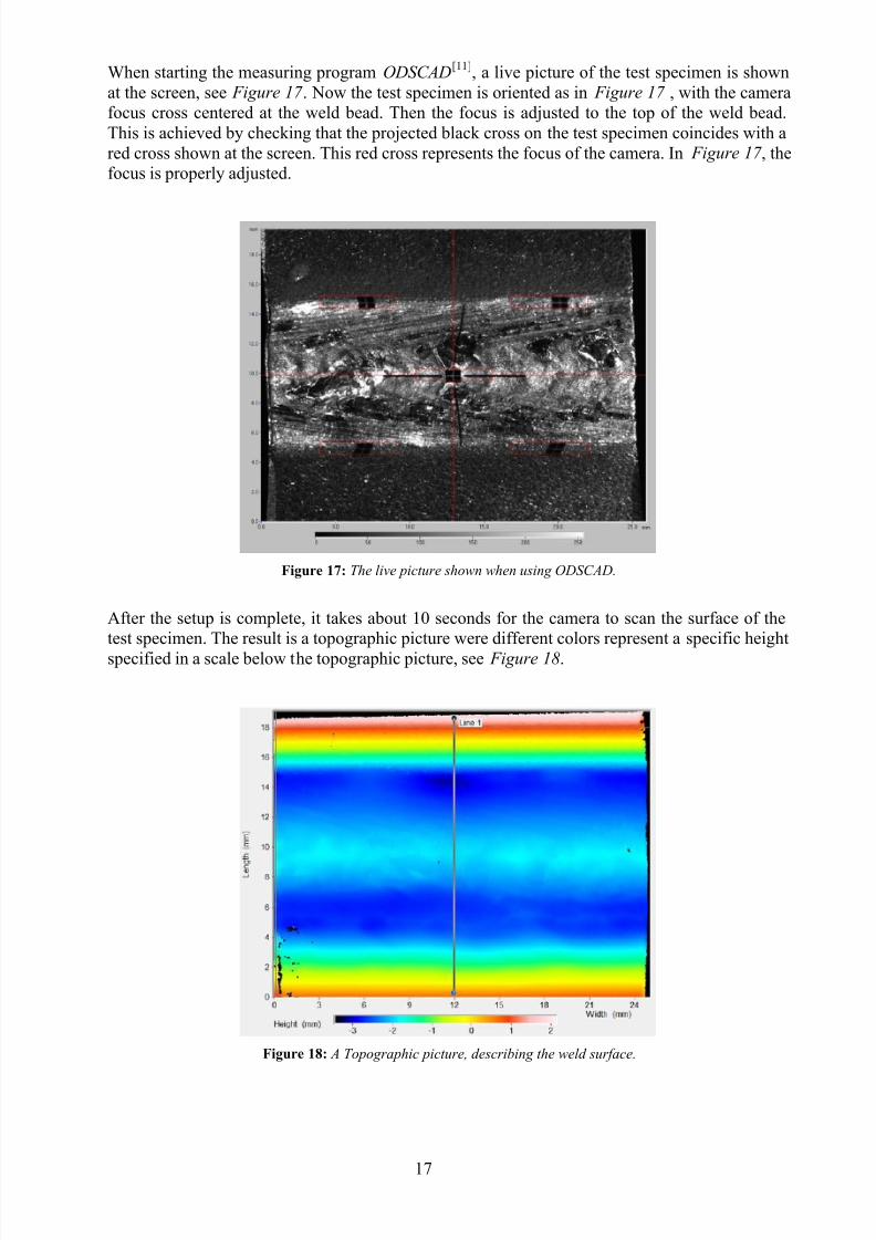
3.2.2 Performing a measurementTo measure the current test specimens – the cruciform joint, see Figure 2 – they were placedunderneath the camera as in Figure 16 .
Figure 16: The setup when measuring the test specimens.
7/28/2019 Fulltext01 Chapter 4
http://slidepdf.com/reader/full/fulltext01-chapter-4 19/80
17
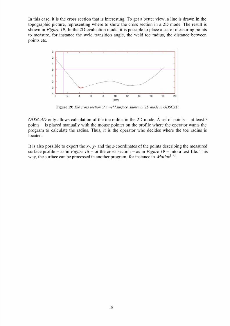
When starting the measuring program ODSCAD[11], a live picture of the test specimen is shown
at the screen, see Figure 17 . Now the test specimen is oriented as in Figure 17 , with the camerafocus cross centered at the weld bead. Then the focus is adjusted to the top of the weld bead.This is achieved by checking that the projected black cross on the test specimen coincides with ared cross shown at the screen. This red cross represents the focus of the camera. In Figure 17 , thefocus is properly adjusted.
Figure 17: The live picture shown when using ODSCAD.
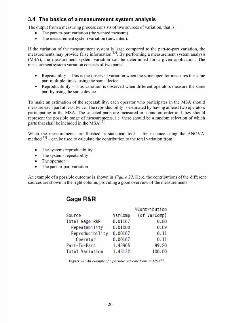
After the setup is complete, it takes about 10 seconds for the camera to scan the surface of thetest specimen. The result is a topographic picture were different colors represent a specific heightspecified in a scale below the topographic picture, see Figure 18.
Figure 18: A Topographic picture, describing the weld surface.
7/28/2019 Fulltext01 Chapter 4
http://slidepdf.com/reader/full/fulltext01-chapter-4 20/80
18
In this case, it is the cross section that is interesting. To get a better view, a line is drawn in thetopographic picture, representing where to show the cross section in a 2D mode. The result isshown in Figure 19. In the 2D evaluation mode, it is possible to place a set of measuring pointsto measure, for instance the weld transition angle, the weld toe radius, the distance between
points etc.
Figure 19: The cross section of a weld surface, shown in 2D mode in ODSCAD.
ODSCAD only allows calculation of the toe radius in the 2D mode. A set of points – at least 3 points – is placed manually with the mouse pointer on the profile where the operator wants the program to calculate the radius. Thus, it is the operator who decides where the toe radius islocated.
It is also possible to export the x-, y- and the z-coordinates of the points describing the measuredsurface profile – as in Figure 18 – or the cross section – as in Figure 19 – into a text file. Thisway, the surface can be processed in another program, for instance in Matlab
[12].

7/28/2019 Fulltext01 Chapter 4
http://slidepdf.com/reader/full/fulltext01-chapter-4 21/80
19
3.3 The Olympus LEXT OLS3000
This measurement system is a confocal laser scanning microscope with a built-in light opticalmicroscope, which is an excellent tool to quantify a surface geometry and topography, see
Figure 20. The technique also provides opportunities to obtain 3D-pictures to assist the highaccuracy measuring, see Figure 21. The specification about the measuring system is listed in
Table 3.
Table 3: The specification of Olympus LEXT OLS3000.
Laser 408nm LD Laser / Class2
Objective 5x, 10x, 20x, 50x, 100x
Optical zoom 1x – 6x
Total magnification 50x – 14400x
Field of view 21 x 21 µm
Number of meas. points 2560 x 2560Lateral Resolution 0.12 µm
Vertical Resolution (height) < 0.01 µm
It is possible to use the system to evaluate surface defects, tool wear, fracture surfaces, etc. Themethod is non-destructive and there is no need for pre-prepared test specimens. Thismeasurement system will only be used in this thesis to compare the measurements between thetwo vision systems and hopefully show that the algorithm described in Chapter 4 has a stablesurface evaluation.
Figure 20: The setup of Olympus LEXT OLS3000.
Figure 21: A 3D-picture of a weld toe.
7/28/2019 Fulltext01 Chapter 4
http://slidepdf.com/reader/full/fulltext01-chapter-4 22/80
20
3.4 The basics of a measurement system analysis
The output from a measuring process consists of two sources of variation, that is: The part-to-part variation (the wanted measure). The measurement system variation (unwanted).
If the variation of the measurement system is large compared to the part-to-part variation, the
measurements may provide false information
[13]
. By performing a measurement system analysis(MSA), the measurement system variation can be determined for a given application. Themeasurement system variation consists of two parts:
Repeatability – This is the observed variation when the same operator measures the same part multiple times, using the same device.
Reproducibility – This variation is observed when different operators measure the same part by using the same device.
To make an estimation of the repeatability, each operator who participates in the MSA shouldmeasure each part at least twice. The reproducibility is estimated by having at least two operators
participating in the MSA. The selected parts are measured in a random order and they shouldrepresent the possible range of measurements, i.e. there should be a random selection of which parts that shall be included in the MSA[13].
When the measurements are finished, a statistical tool – for instance using the ANOVA-method[13] – can be used to calculate the contribution to the total variation from:
The systems reproducibility The systems repeatability The operator The part-to-part variation
An example of a possible outcome is shown in Figure 22. Here, the contributions of the differentsources are shown in the right column, providing a good overview of the measurements.
Figure 22: An example of a possible outcome from an MSA[13].
7/28/2019 Fulltext01 Chapter 4
http://slidepdf.com/reader/full/fulltext01-chapter-4 23/80
21
3.5 Measuring operation
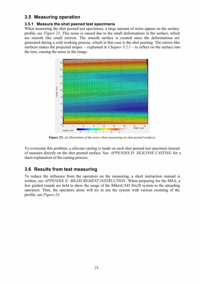
3.5.1 Measure the shot peened test specimensWhen measuring the shot peened test specimens, a large amount of noise appear on the surface
profile, see Figure 23. This noise is caused due to the small deformations in the surface, whichare smooth like small mirrors. The smooth surface is created since the deformations aregenerated during a cold working process, which in this case is the shot peening. The mirror-likesurfaces makes the projected stripes – explained in Chapter 3.2.1 – to reflect on the surface intothe lens, causing the noise in the image.
Figure 23: An illustration of the noise when measuring on shot peened surfaces.
To overcome this problem, a silicone casting is made on each shot peened test specimen insteadof measure directly on the shot peened surface. See APPENDIX D: SILICONE CASTING for ashort explanation of the casting process.
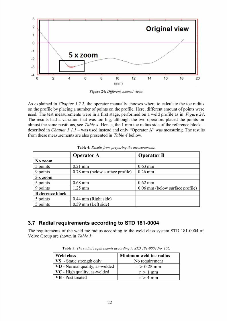
3.6 Results from test measuring
To reduce the influence from the operators on the measuring, a short instruction manual iswritten, see APPENDIX E: MEASUREMENT INSTRUCTION . When preparing for the MSA, afew guided rounds are held to show the usage of the MikroCAD 26x20 system to the attendingoperators. Thus, the operators alone will try to use the system with various zooming of the
profile, see Figure 24.
7/28/2019 Fulltext01 Chapter 4
http://slidepdf.com/reader/full/fulltext01-chapter-4 24/80
22
Figure 24: Different zoomed views.
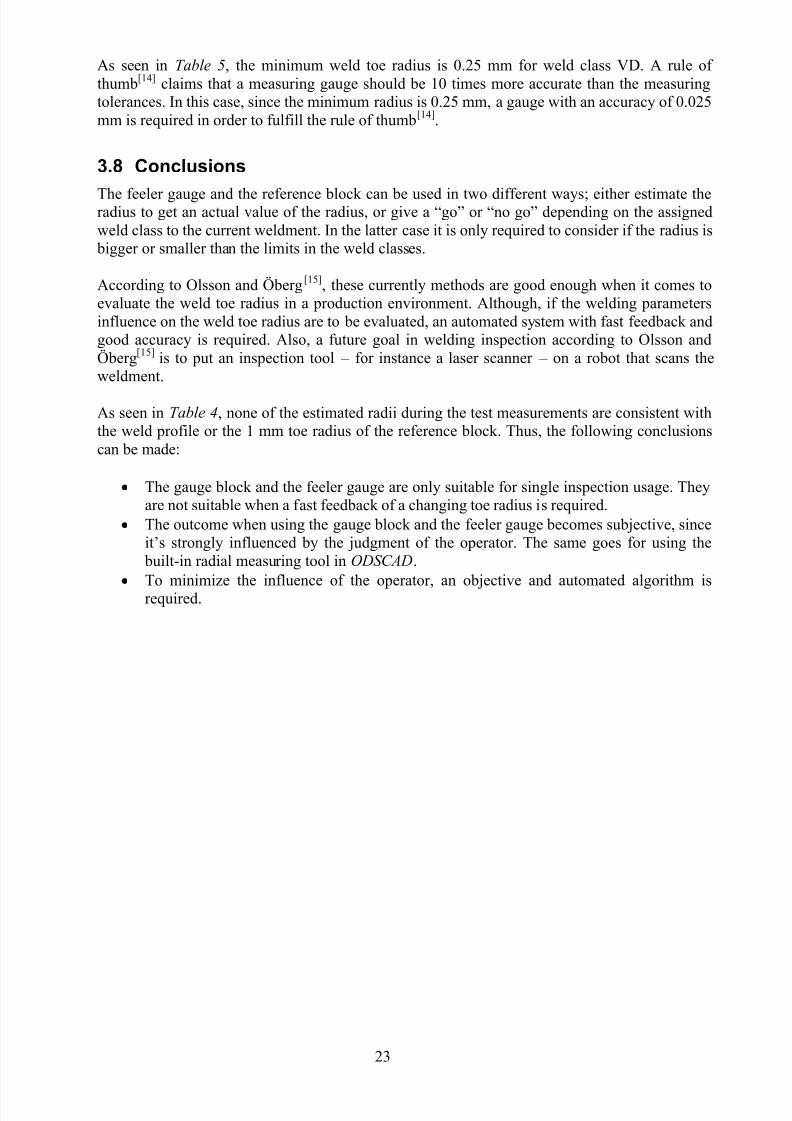
As explained in Chapter 3.2.2, the operator manually chooses where to calculate the toe radiuson the profile by placing a number of points on the profile. Here, different amount of points wereused. The test measurements were in a first stage, performed on a weld profile as in Figure 24. The results had a variation that was too big, although the two operators placed the points onalmost the same positions, see Table 4. Hence, the 1 mm toe radius side of the reference block – described in Chapter 3.1.1 – was used instead and only “O perator A” was measuring. The resultsfrom these measurements are also presented in Table 4 bellow.
Table 4: Results from preparing the measurements.
Operator A Operator BNo zoom
5 points 0.21 mm 0.63 mm9 points 0.78 mm (below surface profile) 0.26 mm5 x zoom
5 points 0.68 mm 0.62 mm9 points 1.25 mm 0.06 mm (below surface profile)Reference block
5 points 0.44 mm (Right side)5 points 0.59 mm (Left side)
3.7 Radial requirements according to STD 181-0004The requirements of the weld toe radius according to the weld class system STD 181-0004 of Volvo Group are shown in Table 5:
Table 5: The radial requirements according to STD 181-0004 No. 106.
Weld class Minimum weld toe radius
VS - Static strength only No requirementVD - Normal quality, as-welded VC - High quality, as-welded VB - Post treated
7/28/2019 Fulltext01 Chapter 4
http://slidepdf.com/reader/full/fulltext01-chapter-4 25/80
23
As seen in Table 5, the minimum weld toe radius is 0.25 mm for weld class VD. A rule of thumb[14] claims that a measuring gauge should be 10 times more accurate than the measuringtolerances. In this case, since the minimum radius is 0.25 mm, a gauge with an accuracy of 0.025mm is required in order to fulfill the rule of thumb[14].
3.8 Conclusions
The feeler gauge and the reference block can be used in two different ways; either estimate theradius to get an actual value of the radius, or give a “go” or “no go” depending on the assigned
weld class to the current weldment. In the latter case it is only required to consider if the radius is bigger or smaller than the limits in the weld classes.
According to Olsson and Öberg[15], these currently methods are good enough when it comes toevaluate the weld toe radius in a production environment. Although, if the welding parametersinfluence on the weld toe radius are to be evaluated, an automated system with fast feedback andgood accuracy is required. Also, a future goal in welding inspection according to Olsson andÖberg[15] is to put an inspection tool – for instance a laser scanner – on a robot that scans theweldment.
As seen in Table 4, none of the estimated radii during the test measurements are consistent withthe weld profile or the 1 mm toe radius of the reference block. Thus, the following conclusionscan be made:
The gauge block and the feeler gauge are only suitable for single inspection usage. Theyare not suitable when a fast feedback of a changing toe radius is required.
The outcome when using the gauge block and the feeler gauge becomes subjective, sinceit’s strongly influenced by the judgment of the operator. The same goes for using the
built-in radial measuring tool in ODSCAD. To minimize the influence of the operator, an objective and automated algorithm is
required.
7/28/2019 Fulltext01 Chapter 4
http://slidepdf.com/reader/full/fulltext01-chapter-4 26/80

7/28/2019 Fulltext01 Chapter 4
http://slidepdf.com/reader/full/fulltext01-chapter-4 27/80
25
WereThe index number of the current point
The total number of points in the cross section
The index number of the current cross section
The total number of cross sections of the surface
i
g
j
c
4.2 Flow chart of the algorithm
The algorithm treats one cross section at a time, stores the data of any identified radii and thenmoves on to the next cross section, i.e. a new y-value. Figure 27 shows a principal flow chart of the algorithm.
Figure 27: A principal flow chart of the algorithm.
4.3 Calculating the radius of a circle
Based on a set of data points arranged as a circle, the radius can – as in Equ. (1) – be calculated
by using the formula given by Råde
[16]
and is illustrated in Figure 28:
2 2 2 x a y b R
(1)
Were
, The cordinates of the center point
, The cordinates of the arc point
The arc radius
a b
x y
R
Figure 28: The description of a circle.
Yes
No

7/28/2019 Fulltext01 Chapter 4
http://slidepdf.com/reader/full/fulltext01-chapter-4 28/80
26
Since Equ. (1) has 3 unknown constants , a minimum of 3 points are required todetermine these constants. However, if the set of data points is larger than 3 points and those
points are not perfectly arranged as a circle, a method for curve fitting is needed. One method touse is named the least square method.
4.3.1 The least square method
The least square method is a mathematical method that can be used to find the best fit of afunction or a curve to a large set of data points. This is called to solve an over-determinedequation system according to Eriksson[17].
Start by rewriting Equ. (1):
2 2 2 x a y b R
Perform the following replacement: 2 2 2
1
2
3
2
2
R a b C
a C
b C
c (2)
Write Equ. (2) in the form of a matrix:
2 21 1 1 1 1
2
2 2
3
1
1 n n n n
c A B
x y C x y
C A c B
x y C x y
If the number of points is greater than 3 , the equation system is written as , nosolution exists that will satisfy all the equations. The solution that provides the best fit, i.e. theminimal mean square error [16], will be provided by the following operation according to theGauss Theorem[16]:
Solve the equation by calculating c :
[]
Finally, calculate R by using Equ. (2).

7/28/2019 Fulltext01 Chapter 4
http://slidepdf.com/reader/full/fulltext01-chapter-4 29/80
27
4.4 Describing the weld geometry as a curvature
Chapter 4.3.1 describes how to calculate the radius from a set of data points, even though thedata points are not arranged as a perfect circle. The measuring system can provide a set of pointsthat describes a cross section of a welded surface as in Figure 29.
Figure 29: A typical cross section of a fillet weld.
Once all of the data points are gathered, the points that describe the weld toe must be selected.Chapter 3.6 showed that manual selection gives results with a variety from 0.21 mm to 1.25 mmon the same surface profile. Also, different operators define the starting point and the ending
point of the radius differently. Thus, this selection must be automated in order to be consequentand reliable.
According to Frenet’s formulas described by Råde[16], a curve is a straight line if and only if there is no curvature, that is . Therefore, analyzing the curvature κ of the whole weldsurface will probably provide a mathematical description of the curve. The curvature can becalculated by using the following formulas, written by Råde[16]:
( ) ( )
||
is the position vector, which in this case is the coordinates of a data point that describes theweld surface. is the unit tangent vector that describes the tangent of the curve with the length of 1. Both
and
are shown in Figure 30.
7/28/2019 Fulltext01 Chapter 4
http://slidepdf.com/reader/full/fulltext01-chapter-4 30/80
28
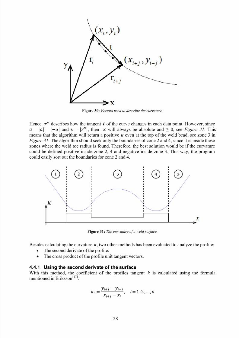
Figure 30: Vectors used to describe the curvature.
Hence, describes how the tangent of the curve changes in each data point. However, since || || and ||, then will always be absolute and ≥ 0, see Figure 31. Thismeans that the algorithm will return a positive even at the top of the weld bead, see zone 3 in
Figure 31. The algorithm should seek only the boundaries of zone 2 and 4, since it is inside thesezones where the weld toe radius is found. Therefore, the best solution would be if the curvaturecould be defined positive inside zone 2, 4 and negative inside zone 3. This way, the programcould easily sort out the boundaries for zone 2 and 4.
Figure 31: The curvature of a weld surface.
Besides calculating the curvature , two other methods has been evaluated to analyze the profile: The second derivate of the profile. The cross product of the profile unit tangent vectors.
4.4.1 Using the second derivate of the surfaceWith this method, the coefficient of the profiles tangent is calculated using the formulamentioned in Eriksson[17]:
7/28/2019 Fulltext01 Chapter 4
http://slidepdf.com/reader/full/fulltext01-chapter-4 31/80
29
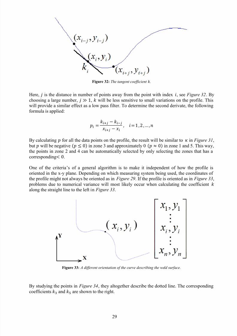
Figure 32: The tangent coefficient .
Here, is the distance in number of points away from the point with index , see Figure 32. Bychoosing a large number, , will be less sensitive to small variations on the profile. Thiswill provide a similar effect as a low pass filter. To determine the second derivate, the followingformula is applied:
By calculating for all the data points on the profile, the result will be similar to in Figure 31, but will be negative in zone 3 and approximately 0 in zone 1 and 5. This way,the points in zone 2 and 4 can be automatically selected by only selecting the zones that has acorresponding .
One of the criteria’s of a general algorithm is to make it independent of how the profile isoriented in the x-y plane. Depending on which measuring system being used, the coordinates of the profile might not always be oriented as in Figure 29. If the profile is oriented as in Figure 33,
problems due to numerical variance will most likely occur when calculating the coefficient along the straight line to the left in Figure 33.
Figure 33: A different orientation of the curve describing the weld surface.
By studying the points in Figure 34, they altogether describe the dotted line. The correspondingcoefficients
and
are shown to the right.

7/28/2019 Fulltext01 Chapter 4
http://slidepdf.com/reader/full/fulltext01-chapter-4 32/80
30
Figure 34: Calculating k along a vertical line.
As seen, the data points in the x-direction are very close to each other. Calculating and gives:
Thus, , and every other along the vertical line will be either very high or very low. Thiswill generate great peaks on the -curve once the whole weld surface is evaluated, which makesit difficult to decide whether it is an area similar to zone 2 and 4 in Figure 31. Therefore, another method is required in order to make the algorithm more flexible due to the orientation of the
profile.
4.4.2 The cross product of the unit tangent vectorsThis method is similar to calculate the curvature , but instead of calculating the difference of as , the cross product between and is calculated. The results of a weld surface that isturning upwards – as in zone 2 and 4 in Figure 31 – is a positive cross product, see Figure 35.
Figure 35: The cross product on a curve turning upwards.
In turn, if the weld surface is turning downwards – as the weld bead (zone 3) in Figure 31 – thevalue of the cross product is negative, see Figure 36 .
7/28/2019 Fulltext01 Chapter 4
http://slidepdf.com/reader/full/fulltext01-chapter-4 33/80
31
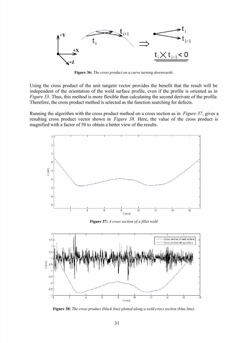
Figure 36: The cross product on a curve turning downwards.
Using the cross product of the unit tangent vector provides the benefit that the result will beindependent of the orientation of the weld surface profile, even if the profile is oriented as in
Figure 33. Thus, this method is more flexible than calculating the second derivate of the profile.Therefore, the cross product method is selected as the function searching for defects.
Running the algorithm with the cross product method on a cross section as in Figure 37 , gives a
resulting cross product vector shown in Figure 38. Here, the value of the cross product ismagnified with a factor of 50 to obtain a better view of the results.
Figure 37: A cross section of a fillet weld.
Figure 38: The cross product (black line) plotted along a weld cross section (blue line).

7/28/2019 Fulltext01 Chapter 4
http://slidepdf.com/reader/full/fulltext01-chapter-4 34/80
32
As seen in Figure 38, a filter is needed in order to find the overall trend of the cross productinside the zone of 2 to 4 mm and 10 to 14 mm along the x-axis.
4.5 Using a filter
By studying the cross product – the black line in Figure 38 – a subtle, positive trend can be
found in the area between 2 to 4 mm and 10 to 14 mm along the x-axis. The noise on the cross product is high frequent, since it makes the line oscillate with a high frequency. To remove thenoise, a low pass filter is required. A low pass filter removes high frequent signals, but it allowslow frequent signals to pass through and form a new signal. This operation is also known as
smoothing according to Aguado and Nixon[18]. The filter is a Gaussian distribution filter and thefunction is described below.
First, a set i of elements – also called scope – are selected from the vector that contains allthe cross product values.
Then – according to Yuan[19] – a weight function creates a set of coefficients based on:
σ , which is the standard deviation of the Gaussian distribution (also known as the normaldistribution), see Figure 39. A small σ will weigh the centered elements more than the
peripheral elements. The larger σ , the more will the scoped elements be weighted equally. The number of elements included in the scope, also called the scope width. A larger
scope width will smooth and reduce peaks more than a smaller scope width. The location of the single element in the scope. The more centered the elements are the
higher they are weighted than the peripheral elements.
√
Figure 39: The Gauss distribution.
Then the coefficients are multiplied with the scoped elements and summarized into a newfiltered value,
.
7/28/2019 Fulltext01 Chapter 4
http://slidepdf.com/reader/full/fulltext01-chapter-4 35/80
33
∑
∑ √
When finished, the scope window is moved towards a step and new elements are selected for anew filtering process. This means that the new scope contains the following elements:
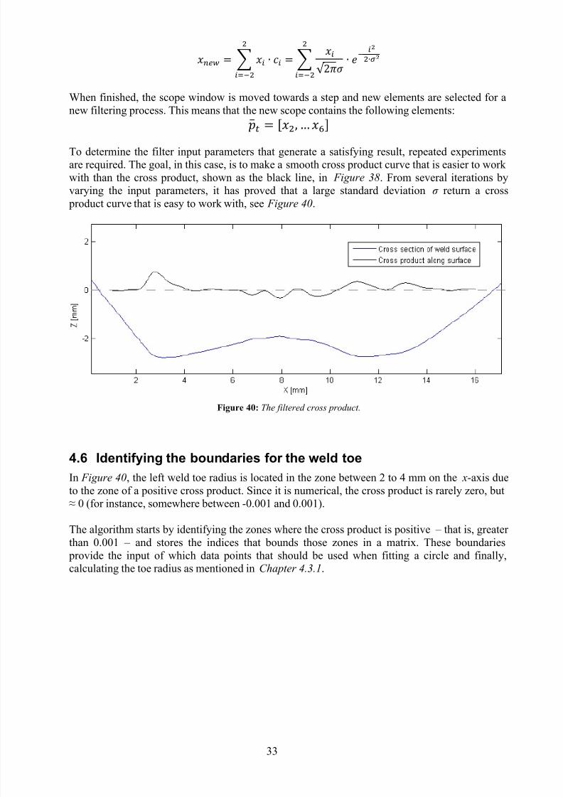
To determine the filter input parameters that generate a satisfying result, repeated experimentsare required. The goal, in this case, is to make a smooth cross product curve that is easier to work with than the cross product, shown as the black line, in Figure 38. From several iterations byvarying the input parameters, it has proved that a large standard deviation σ return a cross
product curve that is easy to work with, see Figure 40.
Figure 40: The filtered cross product.
4.6 Identifying the boundaries for the weld toe
In Figure 40, the left weld toe radius is located in the zone between 2 to 4 mm on the x-axis dueto the zone of a positive cross product. Since it is numerical, the cross product is rarely zero, but≈ 0 (for instance, somewhere between -0.001 and 0.001).
The algorithm starts by identifying the zones where the cross product is positive – that is, greater than 0.001 – and stores the indices that bounds those zones in a matrix. These boundaries
provide the input of which data points that should be used when fitting a circle and finally,calculating the toe radius as mentioned in Chapter 4.3.1.
7/28/2019 Fulltext01 Chapter 4
http://slidepdf.com/reader/full/fulltext01-chapter-4 36/80
34
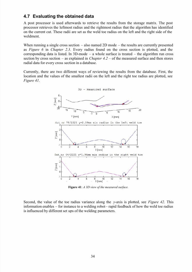
4.7 Evaluating the obtained data
A post processor is used afterwards to retrieve the results from the storage matrix. The post processor retrieves the leftmost radius and the rightmost radius that the algorithm has identifiedon the current cut. These radii are set as the weld toe radius on the left and the right side of theweldment.
When running a single cross section – also named 2D mode – the results are currently presentedas Figure 6 in Chapter 2.3. Every radius found on the cross section is plotted, and thecorresponding data is listed. In 3D-mode – a whole surface is treated – the algorithm run crosssection by cross section – as explained in Chapter 4.2 – of the measured surface and then storesradial data for every cross section in a database.
Currently, there are two different ways of reviewing the results from the database. First, thelocation and the values of the smallest radii on the left and the right toe radius are plotted, see
Figure 41.
Figure 41: A 3D view of the measured surface.
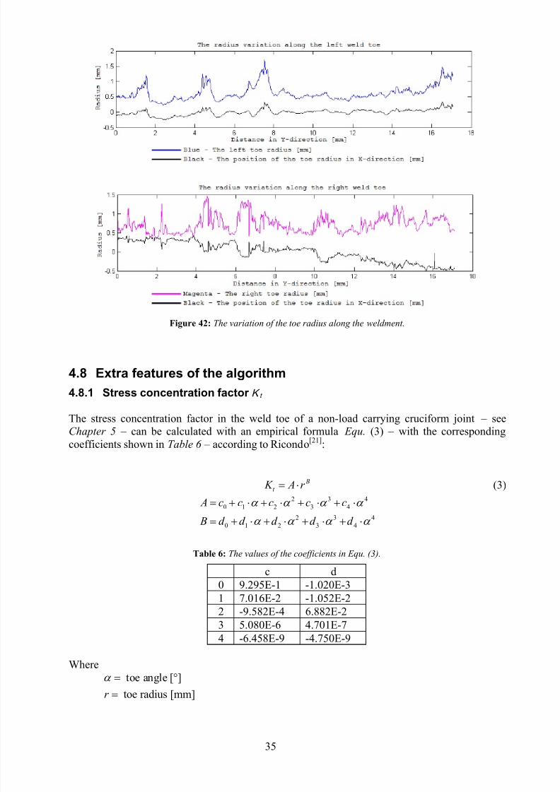
Second, the value of the toe radius variance along the y-axis is plotted, see Figure 42. Thisinformation enables – for instance to a welding robot – rapid feedback of how the weld toe radiusis influenced by different set ups of the welding parameters.
7/28/2019 Fulltext01 Chapter 4
http://slidepdf.com/reader/full/fulltext01-chapter-4 37/80
35
Figure 42: The variation of the toe radius along the weldment.
4.8 Extra features of the algorithm
4.8.1 Stress concentration factor K t
The stress concentration factor in the weld toe of a non-load carrying cruciform joint – seeChapter 5 – can be calculated with an empirical formula Equ. (3) – with the correspondingcoefficients shown in Table 6 – according to Ricondo[21]:
B
t K A r (3)2 3 4
0 1 2 3 4
2 3 4
0 1 2 3 4
A c c c c c
B d d d d d
Table 6: The values of the coefficients in Equ. (3).
c d0 9.295E-1 -1.020E-31 7.016E-2 -1.052E-22 -9.582E-4 6.882E-23 5.080E-6 4.701E-74 -6.458E-9 -4.750E-9
Wheretoe angle [ ]
toe radius [mm]r
7/28/2019 Fulltext01 Chapter 4
http://slidepdf.com/reader/full/fulltext01-chapter-4 38/80
36
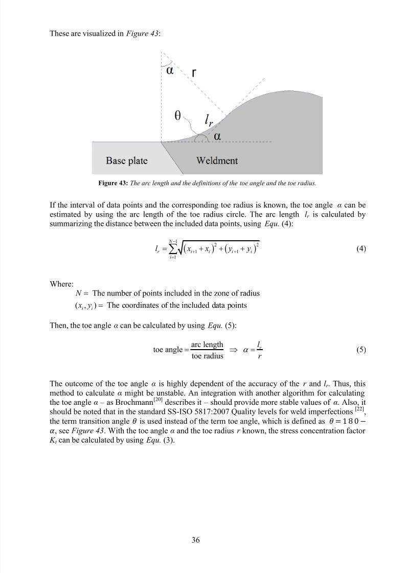
These are visualized in Figure 43:
Figure 43: The arc length and the definitions of the toe angle and the toe radius.
If the interval of data points and the corresponding toe radius is known, the toe angle α can beestimated by using the arc length of the toe radius circle. The arc length l r is calculated bysummarizing the distance between the included data points, using Equ. (4):
1
2 2
1 1
1
N
r i i i i
i
l x x y y
(4)
Where:The number of points included in the zone of radius
( , ) The coordinates of the included data pointsi i
N
x y
Then, the toe angle α can be calculated by using Equ. (5):
arc lengthtoe angle
toe radius
r l
r (5)
The outcome of the toe angle α is highly dependent of the accuracy of the r and l r . Thus, thismethod to calculate α might be unstable. An integration with another algorithm for calculating
the toe angle α – as Brochmann[20] describes it – should provide more stable values of α. Also, itshould be noted that in the standard SS-ISO 5817:2007 Quality levels for weld imperfections [22], the term transition angle is used instead of the term toe angle, which is defined as , see Figure 43. With the toe angle α and the toe radius r known, the stress concentration factor
K t can be calculated by using Equ. (3).
7/28/2019 Fulltext01 Chapter 4
http://slidepdf.com/reader/full/fulltext01-chapter-4 39/80
37
4.9 Results when running the algorithm
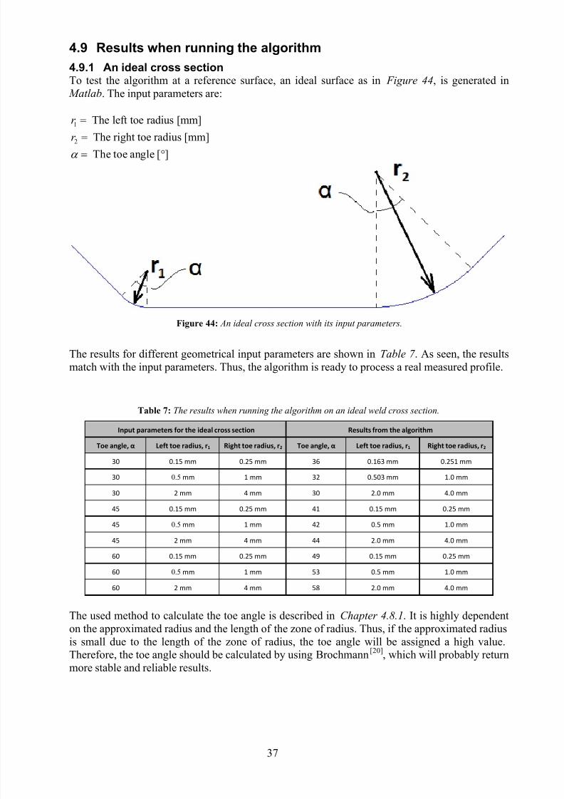
4.9.1 An ideal cross sectionTo test the algorithm at a reference surface, an ideal surface as in Figure 44, is generated in
Matlab. The input parameters are:
1
2
The left toe radius [mm]
The right toe radius [mm]The toe angle [ ]
r
r
Figure 44: An ideal cross section with its input parameters.
The results for different geometrical input parameters are shown in Table 7 . As seen, the resultsmatch with the input parameters. Thus, the algorithm is ready to process a real measured profile.
Table 7: The results when running the algorithm on an ideal weld cross section.
Input parameters for the ideal cross section Results from the algorithm
Toe angle, α Left toe radius, r1 Right toe radius, r2 Toe angle, α Left toe radius, r1 Right toe radius, r2
30 0.15 mm 0.25 mm 36 0.163 mm 0.251 mm
30 0.5 mm 1 mm 32 0.503 mm 1.0 mm
30 2 mm 4 mm 30 2.0 mm 4.0 mm
45 0.15 mm 0.25 mm 41 0.15 mm 0.25 mm
45 0.5 mm 1 mm 42 0.5 mm 1.0 mm
45 2 mm 4 mm 44 2.0 mm 4.0 mm
60 0.15 mm 0.25 mm 49 0.15 mm 0.25 mm
60 0.5 mm 1 mm 53 0.5 mm 1.0 mm
60 2 mm 4 mm 58 2.0 mm 4.0 mm
The used method to calculate the toe angle is described in Chapter 4.8.1. It is highly dependenton the approximated radius and the length of the zone of radius. Thus, if the approximated radiusis small due to the length of the zone of radius, the toe angle will be assigned a high value.Therefore, the toe angle should be calculated by using Brochmann[20], which will probably returnmore stable and reliable results.
7/28/2019 Fulltext01 Chapter 4
http://slidepdf.com/reader/full/fulltext01-chapter-4 40/80
38
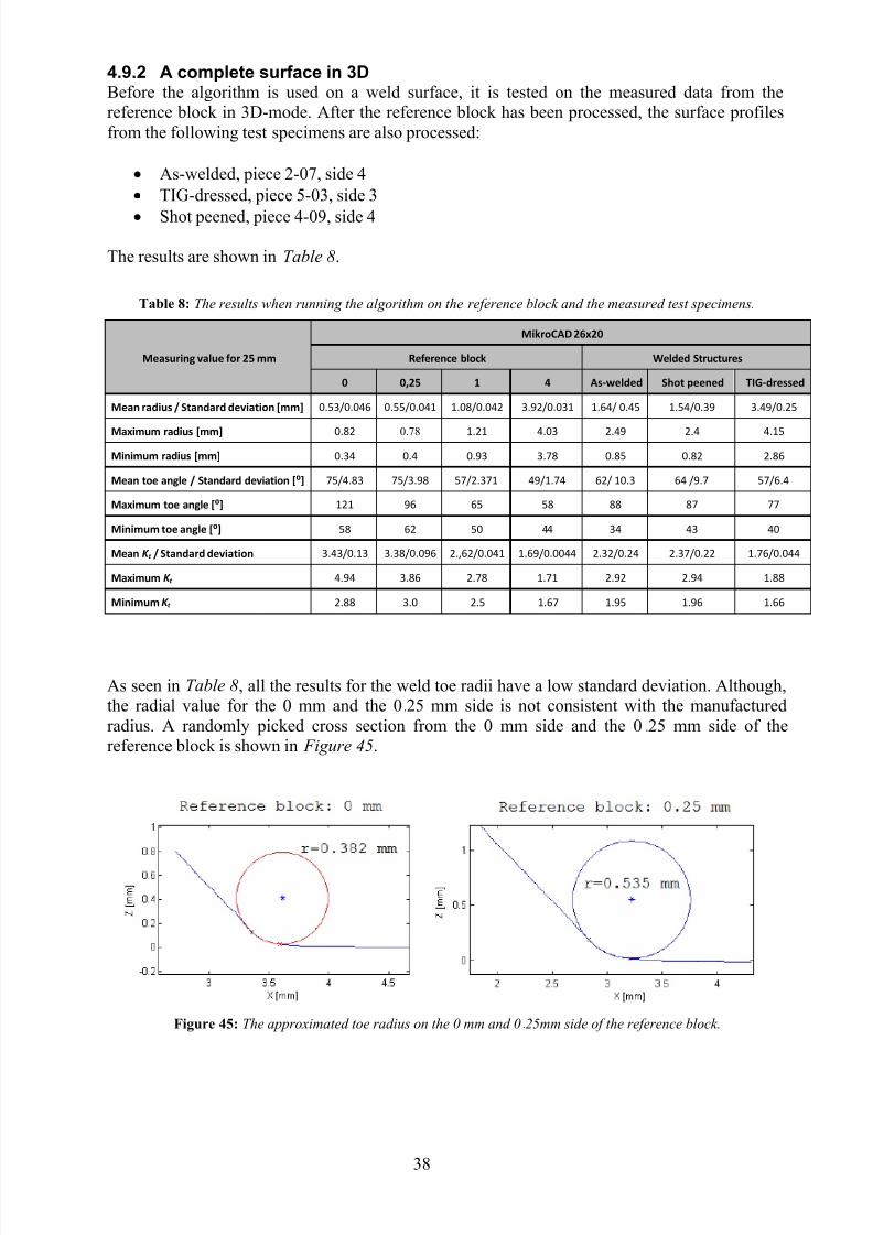
4.9.2 A complete surface in 3DBefore the algorithm is used on a weld surface, it is tested on the measured data from thereference block in 3D-mode. After the reference block has been processed, the surface profilesfrom the following test specimens are also processed:
As-welded, piece 2-07, side 4 TIG-dressed, piece 5-03, side 3
Shot peened, piece 4-09, side 4
The results are shown in Table 8.
Table 8: The results when running the algorithm on the reference block and the measured test specimens.
Measuring value for 25 mm
MikroCAD 26x20
Reference block Welded Structures
0 0,25 1 4 As-welded Shot peened TIG-dressed
Mean radius / Standard deviation [mm] 0.53/0.046 0.55/0.041 1.08/0.042 3.92/0.031 1.64/ 0.45 1.54/0.39 3.49/0.25
Maximum radius [mm] 0.82 0.78 1.21 4.03 2.49 2.4 4.15
Minimum radius [mm] 0.34 0.4 0.93 3.78 0.85 0.82 2.86
Mean toe angle / Standard deviation [⁰] 75/4.83 75/3.98 57/2.371 49/1.74 62/ 10.3 64 /9.7 57/6.4
Maximum toe angle [⁰] 121 96 65 58 88 87 77
Minimum toe angle [⁰] 58 62 50 44 34 43 40
Mean K t / Standard deviation 3.43/0.13 3.38/0.096 2.,62/0.041 1.69/0.0044 2.32/0.24 2.37/0.22 1.76/0.044
Maximum K t 4.94 3.86 2.78 1.71 2.92 2.94 1.88
Minimum K t 2.88 3.0 2.5 1.67 1.95 1.96 1.66
As seen in Table 8, all the results for the weld toe radii have a low standard deviation. Although,the radial value for the 0 mm and the 0.25 mm side is not consistent with the manufacturedradius. A randomly picked cross section from the 0 mm side and the 0.25 mm side of thereference block is shown in Figure 45.
Figure 45: The approximated toe radius on the 0 mm and 0.25mm side of the reference block.
7/28/2019 Fulltext01 Chapter 4
http://slidepdf.com/reader/full/fulltext01-chapter-4 41/80
39
As seen, the approximated radius fits the profile. Possible causes to this phenomenon are:
The precision and accuracy of the wire EDM machine The large diameter (0.17 mm) of the wire.
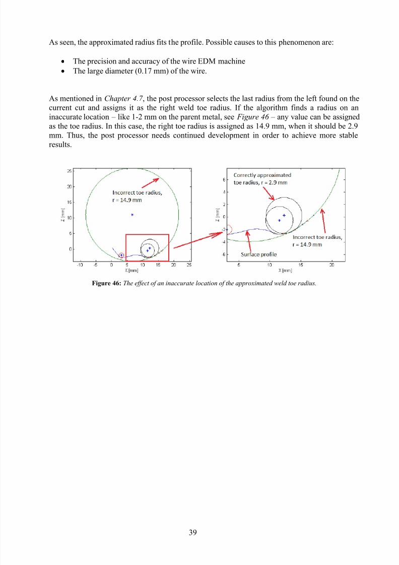
As mentioned in Chapter 4.7 , the post processor selects the last radius from the left found on thecurrent cut and assigns it as the right weld toe radius. If the algorithm finds a radius on aninaccurate location – like 1-2 mm on the parent metal, see Figure 46 – any value can be assignedas the toe radius. In this case, the right toe radius is assigned as 14.9 mm, when it should be 2.9mm. Thus, the post processor needs continued development in order to achieve more stableresults.
Figure 46: The effect of an inaccurate location of the approximated weld toe radius.
7/28/2019 Fulltext01 Chapter 4
http://slidepdf.com/reader/full/fulltext01-chapter-4 42/80
40
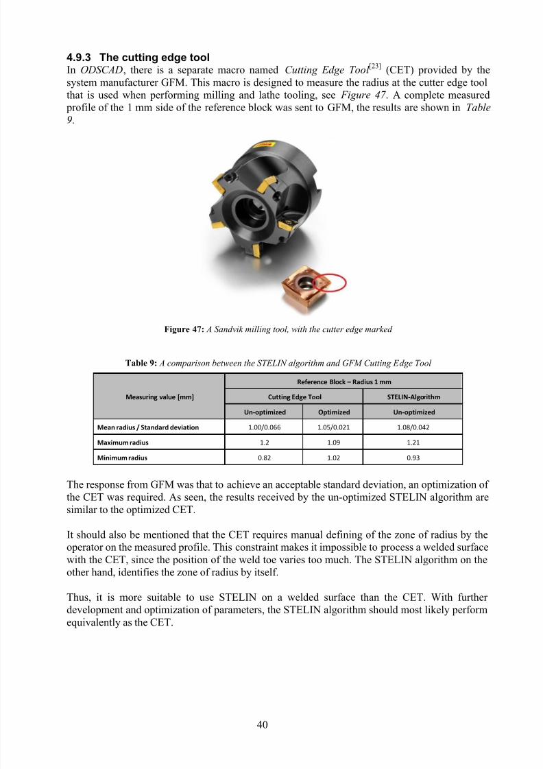
4.9.3 The cutting edge toolIn ODSCAD, there is a separate macro named Cutting Edge Tool
[23] (CET) provided by thesystem manufacturer GFM. This macro is designed to measure the radius at the cutter edge toolthat is used when performing milling and lathe tooling, see Figure 47 . A complete measured
profile of the 1 mm side of the reference block was sent to GFM, the results are shown in Table
9.
Figure 47: A Sandvik milling tool, with the cutter edge marked
Table 9: A comparison between the STELIN algorithm and GFM Cutting Edge Tool
Measuring value [mm]
Reference Block – Radius 1 mm
Cutting Edge Tool STELIN-Algorithm
Un-optimized Optimized Un-optimized
Mean radius / Standard deviation 1.00/0.066 1.05/0.021 1.08/0.042
Maximum radius 1.2 1.09 1.21
Minimum radius 0.82 1.02 0.93
The response from GFM was that to achieve an acceptable standard deviation, an optimization of the CET was required. As seen, the results received by the un-optimized STELIN algorithm aresimilar to the optimized CET.
It should also be mentioned that the CET requires manual defining of the zone of radius by theoperator on the measured profile. This constraint makes it impossible to process a welded surfacewith the CET, since the position of the weld toe varies too much. The STELIN algorithm on theother hand, identifies the zone of radius by itself.
Thus, it is more suitable to use STELIN on a welded surface than the CET. With further development and optimization of parameters, the STELIN algorithm should most likely performequivalently as the CET.
7/28/2019 Fulltext01 Chapter 4
http://slidepdf.com/reader/full/fulltext01-chapter-4 43/80
41
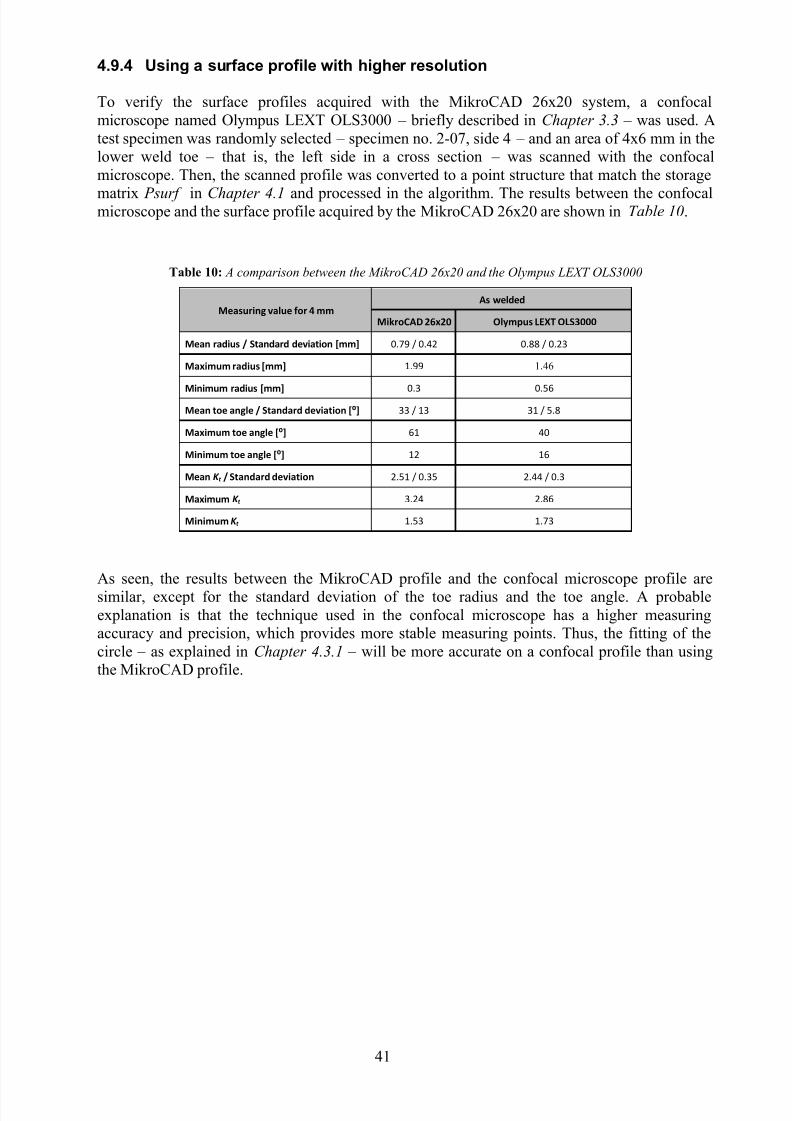
4.9.4 Using a surface profile with higher resolution
To verify the surface profiles acquired with the MikroCAD 26x20 system, a confocalmicroscope named Olympus LEXT OLS3000 – briefly described in Chapter 3.3 – was used. Atest specimen was randomly selected – specimen no. 2-07, side 4 – and an area of 4x6 mm in thelower weld toe – that is, the left side in a cross section – was scanned with the confocalmicroscope. Then, the scanned profile was converted to a point structure that match the storage
matrix Psurf in Chapter 4.1 and processed in the algorithm. The results between the confocalmicroscope and the surface profile acquired by the MikroCAD 26x20 are shown in Table 10.
Table 10: A comparison between the MikroCAD 26x20 and the Olympus LEXT OLS3000
Measuring value for 4 mmAs welded
MikroCAD 26x20 Olympus LEXT OLS3000
Mean radius / Standard deviation [mm] 0.79 / 0.42 0.88 / 0.23
Maximum radius [mm] 1.99 1.46
Minimum radius [mm] 0.3 0.56
Mean toe angle / Standard deviation [⁰] 33 / 13 31 / 5.8
Maximum toe angle [⁰] 61 40
Minimum toe angle [⁰] 12 16
Mean K t / Standard deviation 2.51 / 0.35 2.44 / 0.3
Maximum K t 3.24 2.86
Minimum K t 1.53 1.73
As seen, the results between the MikroCAD profile and the confocal microscope profile aresimilar, except for the standard deviation of the toe radius and the toe angle. A probableexplanation is that the technique used in the confocal microscope has a higher measuringaccuracy and precision, which provides more stable measuring points. Thus, the fitting of thecircle – as explained in Chapter 4.3.1 – will be more accurate on a confocal profile than usingthe MikroCAD profile.
7/28/2019 Fulltext01 Chapter 4
http://slidepdf.com/reader/full/fulltext01-chapter-4 44/80
42
5 FATIGUE ASSESSMENT
In this chapter, the theory behind the methods used to predict the fatigue strength today is
presented. Some of the difficulties and weaknesses of the theory are also shown with simulations
and discussion.
The weld quality regarding fatigue and product life depends on the local weld geometry. InVolvo Group’s developed weld class system STD 181-0004, different types of imperfections are
prescribed regarding the local weld. Some of the most typical fatigue starting points are sharp toeradii, cold laps and large root cracks. As mentioned earlier, only the toe radius has beenevaluated in this thesis, to see how the variation of the toe radius is influencing the fatiguestrength. It has been confirmed by Barsoum and Samuelsson[24] that the stress concentrationfactor depends more of the local geometry in the weld toe (radius and angle) instead of the weldthroat size and the weld reinforcement The value of the stress concentration factor increases withan increased plate thickness when the toe radius is held constant. Reduced fatigue strength willthen occur with a large toe angle and a small radius.
A notch/radius in a structure, as mentioned, will have a negative influence on the fatiguestrength, which is called the “Notch effect”. The elastic stress concentration is determined by the
loading and the geometry of the component. The dependence of the geometry is determined bythe materials “microstructural support”, which is independent of the global dimensions and theelastic modulus. The term microstructural support, according to Radaj and Sonsino[25] says:
“’microstructural support’ means that the maximum notch stress according to the theory of
elasticity is not decisive for crack initiation and propagation but instead some lower local stress
gained by averaging the maximum stress over a material-characteristic small length, area or
volume at the notch root (explicable from grain structure, microyielding and crack initiation
processes).”
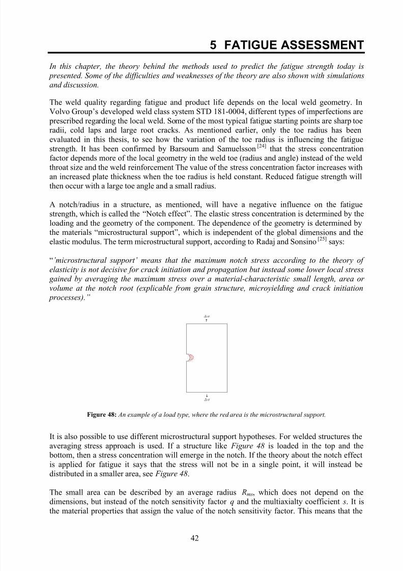
Figure 48: An example of a load type, where the red area is the microstructural support.
It is also possible to use different microstructural support hypotheses. For welded structures theaveraging stress approach is used. If a structure like Figure 48 is loaded in the top and the
bottom, then a stress concentration will emerge in the notch. If the theory about the notch effectis applied for fatigue it says that the stress will not be in a single point, it will instead bedistributed in a smaller area, see Figure 48.
The small area can be described by an average radius Rms, which does not depend on the
dimensions, but instead of the notch sensitivity factor q and the multiaxialty coefficient s. It isthe material properties that assign the value of the notch sensitivity factor. This means that the
7/28/2019 Fulltext01 Chapter 4
http://slidepdf.com/reader/full/fulltext01-chapter-4 45/80
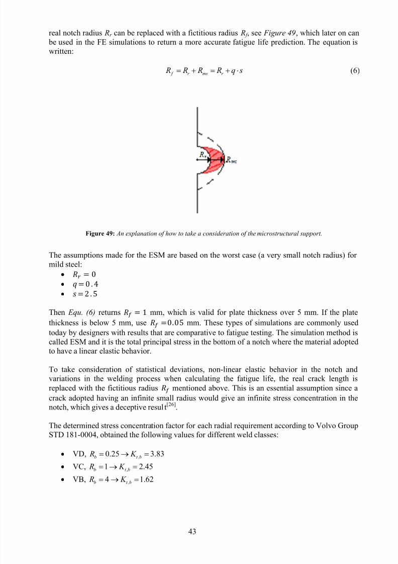
43
real notch radius Rr can be replaced with a fictitious radius R f , see Figure 49, which later on can be used in the FE simulations to return a more accurate fatigue life prediction. The equation iswritten:
f r ms r R R R R q s (6)
Figure 49: An explanation of how to take a consideration of the microstructural support.
The assumptions made for the ESM are based on the worst case (a very small notch radius) for mild steel:
Then Equ. (6) returns mm, which is valid for plate thickness over 5 mm. If the platethickness is below 5 mm, use mm. These types of simulations are commonly usedtoday by designers with results that are comparative to fatigue testing. The simulation method iscalled ESM and it is the total principal stress in the bottom of a notch where the material adoptedto have a linear elastic behavior.
To take consideration of statistical deviations, non-linear elastic behavior in the notch andvariations in the welding process when calculating the fatigue life, the real crack length isreplaced with the fictitious radius
mentioned above. This is an essential assumption since a
crack adopted having an infinite small radius would give an infinite stress concentration in thenotch, which gives a deceptive result[26].
The determined stress concentration factor for each radial requirement according to Volvo GroupSTD 181-0004, obtained the following values for different weld classes:
VD, ,0.25 3.83b t b R K
VC, ,1 2.45b t b R K
VB, ,4 1.62b t b R K
7/28/2019 Fulltext01 Chapter 4
http://slidepdf.com/reader/full/fulltext01-chapter-4 46/80
44
Note: The ESM is not used here since it is the influence of the real radii that shall be studied, sothis will be used as reference values later on in this chapter.
5.1 Location of surface inhomogeneity
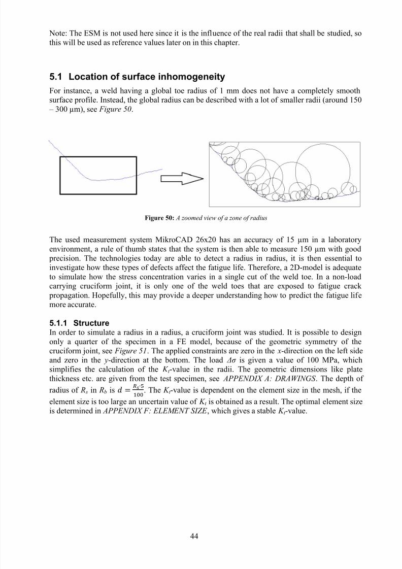
For instance, a weld having a global toe radius of 1 mm does not have a completely smooth
surface profile. Instead, the global radius can be described with a lot of smaller radii (around 150 – 300 µm), see Figure 50.
Figure 50: A zoomed view of a zone of radius
The used measurement system MikroCAD 26x20 has an accuracy of 15 µm in a laboratoryenvironment, a rule of thumb states that the system is then able to measure 150 µm with good
precision. The technologies today are able to detect a radius in radius, it is then essential toinvestigate how these types of defects affect the fatigue life. Therefore, a 2D-model is adequateto simulate how the stress concentration varies in a single cut of the weld toe. In a non-loadcarrying cruciform joint, it is only one of the weld toes that are exposed to fatigue crack
propagation. Hopefully, this may provide a deeper understanding how to predict the fatigue lifemore accurate.
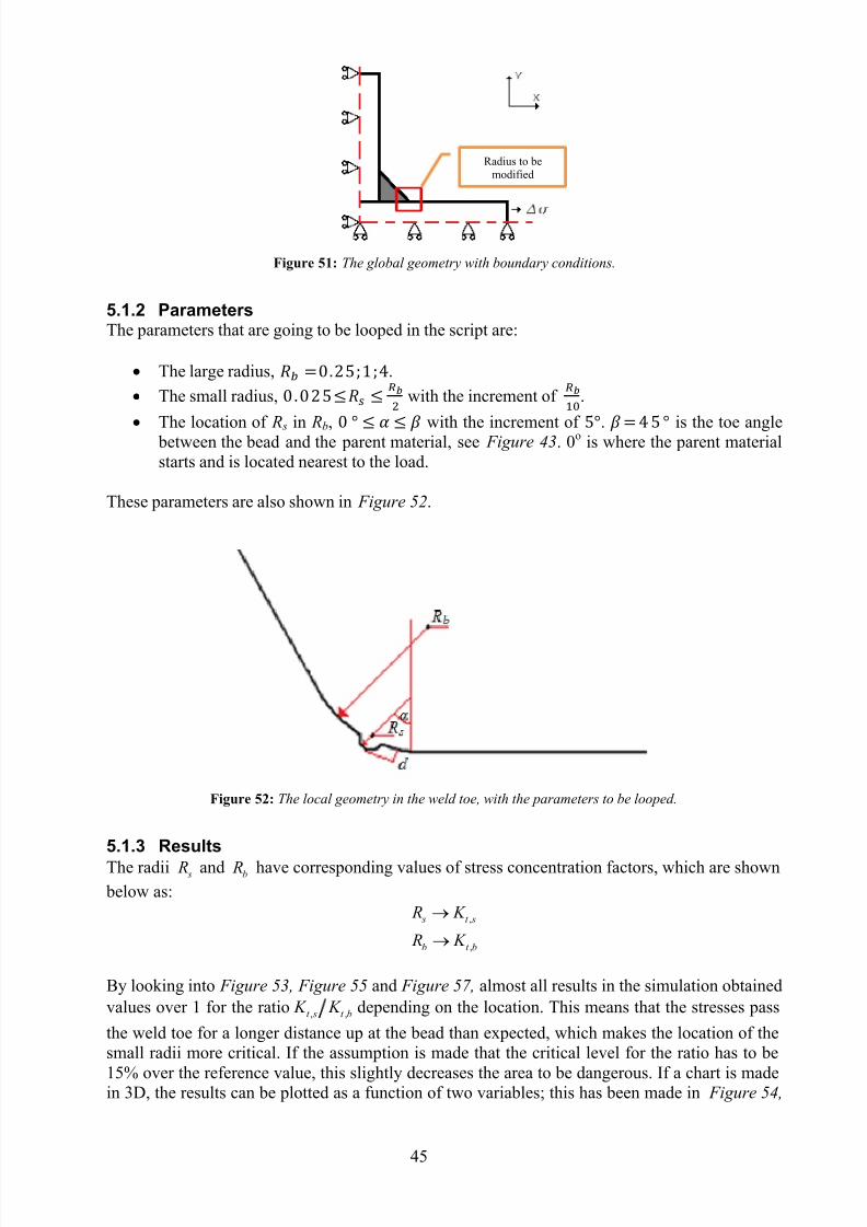
5.1.1 StructureIn order to simulate a radius in a radius, a cruciform joint was studied. It is possible to designonly a quarter of the specimen in a FE model, because of the geometric symmetry of thecruciform joint, see Figure 51. The applied constraints are zero in the x-direction on the left sideand zero in the y-direction at the bottom. The load Δσ is given a value of 100 MPa, whichsimplifies the calculation of the K t -value in the radii. The geometric dimensions like platethickness etc. are given from the test specimen, see APPENDIX A: DRAWINGS . The depth of
radius of R s in Rb is
. The K t -value is dependent on the element size in the mesh, if the
element size is too large an uncertain value of K t is obtained as a result. The optimal element sizeis determined in APPENDIX F: ELEMENT SIZE , which gives a stable K t -value.
7/28/2019 Fulltext01 Chapter 4
http://slidepdf.com/reader/full/fulltext01-chapter-4 47/80
45
Figure 51: The global geometry with boundary conditions.
5.1.2 ParametersThe parameters that are going to be looped in the script are:
The large radius, .
The small radius, with the increment of .
The location of R s in Rb, with the increment of . is the toe angle between the bead and the parent material, see Figure 43. 0o is where the parent materialstarts and is located nearest to the load.
These parameters are also shown in Figure 52.
Figure 52: The local geometry in the weld toe, with the parameters to be looped.
5.1.3 Results
The radii s R and b R have corresponding values of stress concentration factors, which are shown
below as:
,
,
s t s
b t b
R K
R K
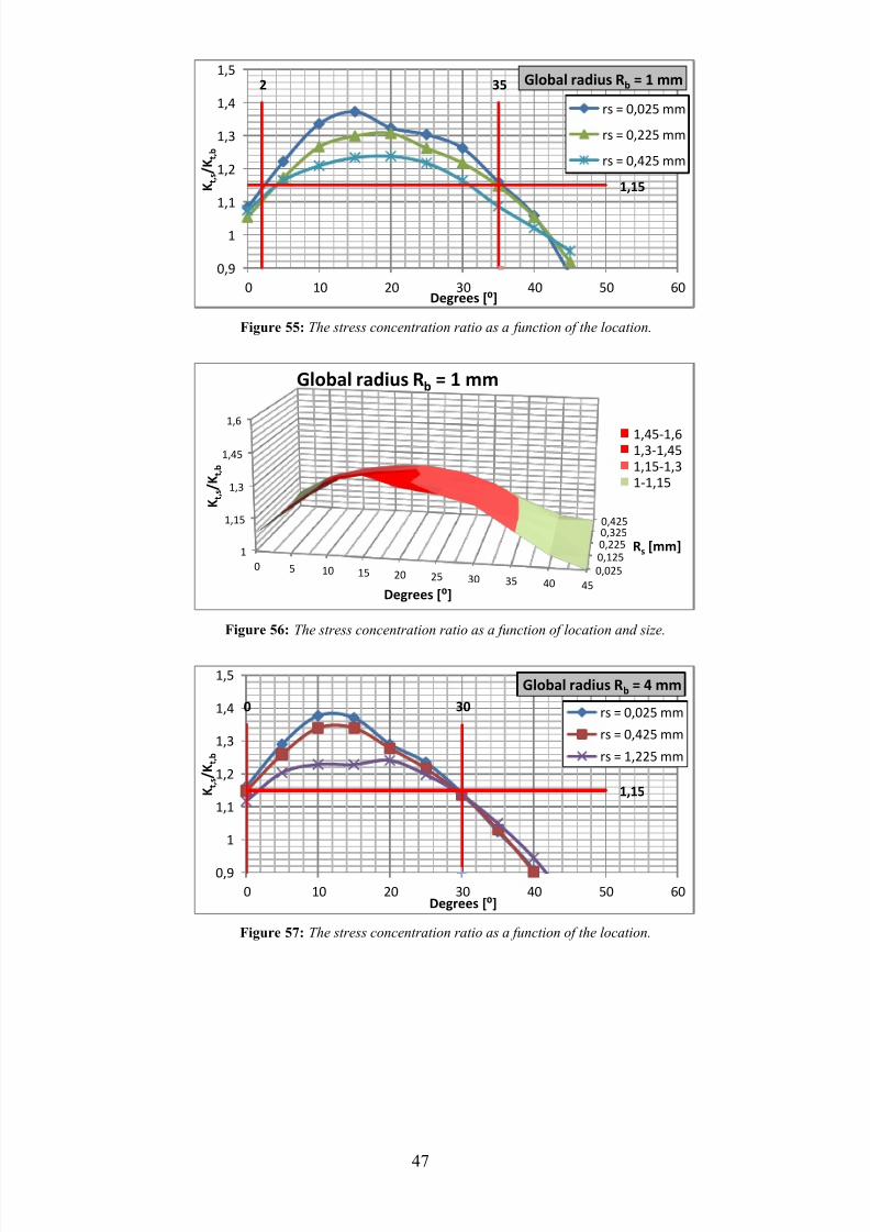
By looking into Figure 53, Figure 55 and Figure 57, almost all results in the simulation obtainedvalues over 1 for the ratio , ,t s t b
K K depending on the location. This means that the stresses pass
the weld toe for a longer distance up at the bead than expected, which makes the location of thesmall radii more critical. If the assumption is made that the critical level for the ratio has to be
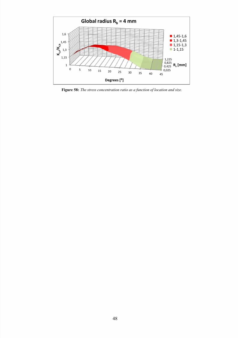
15% over the reference value, this slightly decreases the area to be dangerous. If a chart is madein 3D, the results can be plotted as a function of two variables; this has been made in Figure 54,
Radius to bemodified

7/28/2019 Fulltext01 Chapter 4
http://slidepdf.com/reader/full/fulltext01-chapter-4 48/80
46
Figure 56 and Figure 58. In the 3D-chart, a better visualization is made of the critical zones, thisgives a Go (green) or No-Go (red) decision.
By observing the charts, the results are relatively stable for each case. The location of where thesmall radius is critical does not change when changing the value of the global radius. Thus, thesmall radii are probably more necessary to find when performing the quality inspection in
production. Also, the weld toe has to be investigated not only in the zone closest to the high
stresses, but also in the zone of the global radius. So far, this simulation has only shown a needfor further investigation and how this surface inhomogeneity should be taken in consideration.
Figure 53: The stress concentration ratio as a function of the location.
Figure 54: The stress concentration ratio as a function of location and size.
1,15
365
0,9
1
1,1
1,2
1,3
1,4
1,5
1,6
0 10 20 30 40 50 60
K t , s /
K t , b
Degrees [⁰]
Global radius Rb = 0,25 mm
rs = 0,025 mm
rs = 0,075 mm
rs = 0,125 mm
0,025
0,050,0750,10,125
1
1,15
1,3
1,45
1,6
0 5 10 15 20 25 30 35 40 45
Rs [mm]
K t , s /
K t , b
Degrees [⁰]
Global radius Rb = 0,25 mm
1,45-1,6
1,3-1,451,15-1,31-1,15
7/28/2019 Fulltext01 Chapter 4
http://slidepdf.com/reader/full/fulltext01-chapter-4 49/80
47
Figure 55: The stress concentration ratio as a function of the location.
Figure 56: The stress concentration ratio as a function of location and size.
Figure 57: The stress concentration ratio as a function of the location.
1,15
2 35
0,9
1
1,1
1,2
1,3
1,4
1,5
0 10 20 30 40 50 60
K t , s /
K t , b
Degrees [⁰]
Global radius Rb = 1 mm
rs = 0,025 mm
rs = 0,225 mm
rs = 0,425 mm
0,025
0,1250,2250,3250,425
1
1,15
1,3
1,45
1,6
0 5 10 15 20 25 30 35 40 45
Rs [mm]
K t , s /
K t , b
Degrees [⁰]
Global radius Rb = 1 mm
1,45-1,61,3-1,451,15-1,31-1,15
1,15
0 30
0,9
1
1,1
1,2
1,3
1,4
1,5
0 10 20 30 40 50 60
K t , s /
K t , b
Degrees [⁰]
Global radius Rb = 4 mm
rs = 0,025 mm
rs = 0,425 mm
rs = 1,225 mm
7/28/2019 Fulltext01 Chapter 4
http://slidepdf.com/reader/full/fulltext01-chapter-4 50/80
48
Figure 58: The stress concentration ratio as a function of location and size.
0,025
0,4250,8251,225
1
1,15
1,3
1,45
1,6
0 5 10 15 20 25 30 35 40 45
Rs [mm]
K t , s /
K t , b
Degrees [⁰]
Global radius Rb = 4 mm
1,45-1,61,3-1,451,15-1,31-1,15
7/28/2019 Fulltext01 Chapter 4
http://slidepdf.com/reader/full/fulltext01-chapter-4 51/80
49
5.2 Size of surface inhomogeneity
This is a similar case to the simulation in Chapter 5.1, but instead two smaller radii will bemodeled in the global radius. This will probably give recommendations for which one of the tworadii that the designer/inspector should take in consideration or if the global radius always is thedesign factor.
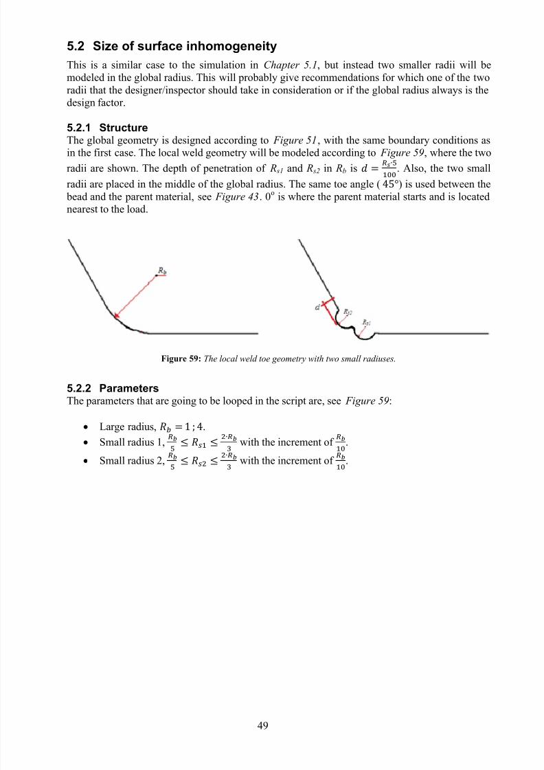
5.2.1 StructureThe global geometry is designed according to Figure 51, with the same boundary conditions asin the first case. The local weld geometry will be modeled according to Figure 59, where the two
radii are shown. The depth of penetration of R s1 and R s2 in Rb is . Also, the two small
radii are placed in the middle of the global radius. The same toe angle () is used between the bead and the parent material, see Figure 43. 0o is where the parent material starts and is locatednearest to the load.
Figure 59: The local weld toe geometry with two small radiuses.
5.2.2 Parameters
The parameters that are going to be looped in the script are, see Figure 59:
Large radius, .
Small radius 1, with the increment of
.
Small radius 2, with the increment of
.
7/28/2019 Fulltext01 Chapter 4
http://slidepdf.com/reader/full/fulltext01-chapter-4 52/80
50
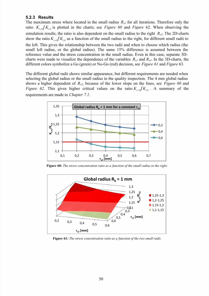
5.2.3 ResultsThe maximum stress where located in the small radius R s1 for all iterations. Therefore only theratio , 1 ,t s t b
K K is plotted in the charts; see Figure 60 and Figure 62. When observing the
simulation results, the ratio is also dependent on the small radius to the right R s2. The 2D-chartsshow the ratio , 1 ,t s t b
K K as a function of the small radius to the right, for different small radii to
the left. This gives the relationship between the two radii and when to choose which radius (thesmall left radius, or the global radius). The same 15% difference is assumed between thereference value and the stress concentration in the small radius. Even in this case, separate 3D-charts were made to visualize the dependence of the variables R s1 and R s2. In the 3D-charts, thedifferent colors symbolize a Go (green) or No-Go (red) decision, see Figure 61 and Figure 63.
The different global radii shows similar appearance, but different requirements are needed whenselecting the global radius or the small radius in the quality inspection. The 4 mm global radiusshows a higher dependent of R s2, because of the lower slope on the lines, see Figure 60 and
Figure 62. This gives higher critical values on the ratio , 1 ,t s t b K K . A summary of the
requirements are made in Chapter 7.1.
Figure 60: The stress concentration ratio as a function of the small radius to the right.
Figure 61: The stress concentration ratio as a function of the two small radii.
1,1
1,15
1,2
1,25
1,3
1,35
0,1 0,2 0,3 0,4 0,5 0,6 0,7
K t , s 1
/ K t , b
rs2 [mm]
Global radius Rb = 1 mm for a constant rs1
0,2
0,4
0,6
0,20,3
0,40,5
0,6
1,1
1,15
1,2
1,25
1,3
0,2 0,3 0,4 0,5 0,6
rs1 [mm]
K t , s 1
/ K t , b
rs2 [mm]
Global radius Rb = 1 mm
1,25-1,3
1,2-1,25
1,15-1,2
1,1-1,15
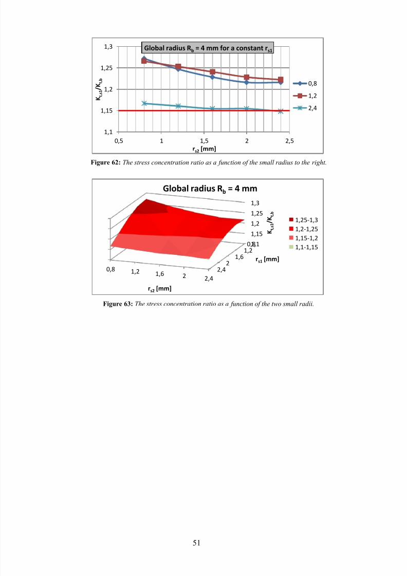
7/28/2019 Fulltext01 Chapter 4
http://slidepdf.com/reader/full/fulltext01-chapter-4 53/80
51
Figure 62: The stress concentration ratio as a function of the small radius to the right.
Figure 63: The stress concentration ratio as a function of the two small radii.
1,1
1,15
1,2
1,25
1,3
0,5 1 1,5 2 2,5
K t , s 1
/ K t , b
rs2 [mm]
Global radius Rb = 4 mm for a constant rs1
0,8
1,2
2,4
0,81,2
1,62
2,4
1,1
1,15
1,2
1,25
1,3
0,8 1,2 1,6 2 2,4
rs1 [mm]
K t , s 1
/ K t , b
rs2 [mm]
Global radius Rb = 4 mm
1,25-1,3
1,2-1,25
1,15-1,2
1,1-1,15
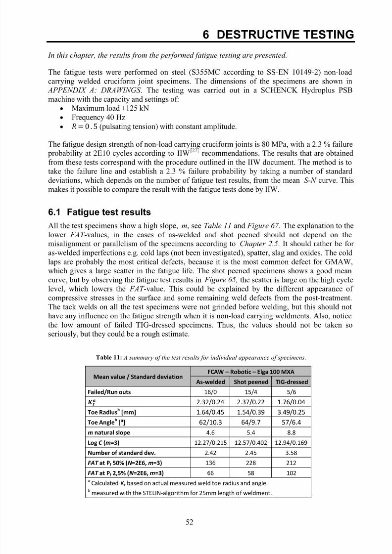
7/28/2019 Fulltext01 Chapter 4
http://slidepdf.com/reader/full/fulltext01-chapter-4 54/80
52
6 DESTRUCTIVE TESTING
In this chapter, the results from the performed fatigue testing are presented.
The fatigue tests were performed on steel (S355MC according to SS-EN 10149-2) non-loadcarrying welded cruciform joint specimens. The dimensions of the specimens are shown in
APPENDIX A: DRAWINGS . The testing was carried out in a SCHENCK Hydroplus PSB
machine with the capacity and settings of: Maximum load ±125 kN
Frequency 40 Hz
(pulsating tension) with constant amplitude.
The fatigue design strength of non-load carrying cruciform joints is 80 MPa, with a 2.3 % failure probability at 2E10 cycles according to IIW[27] recommendations. The results that are obtainedfrom these tests correspond with the procedure outlined in the IIW document. The method is totake the failure line and establish a 2.3 % failure probability by taking a number of standarddeviations, which depends on the number of fatigue test results, from the mean S - N curve. Thismakes it possible to compare the result with the fatigue tests done by IIW.
6.1 Fatigue test results
All the test specimens show a high slope, m, see Table 11 and Figure 67 . The explanation to thelower FAT -values, in the cases of as-welded and shot peened should not depend on themisalignment or parallelism of the specimens according to Chapter 2.5. It should rather be for as-welded imperfections e.g. cold laps (not been investigated), spatter, slag and oxides. The coldlaps are probably the most critical defects, because it is the most common defect for GMAW,which gives a large scatter in the fatigue life. The shot peened specimens shows a good meancurve, but by observing the fatigue test results in Figure 65, the scatter is large on the high cycle
level, which lowers the FAT -value. This could be explained by the different appearance of compressive stresses in the surface and some remaining weld defects from the post-treatment.The tack welds on all the test specimens were not grinded before welding, but this should nothave any influence on the fatigue strength when it is non-load carrying weldments. Also, noticethe low amount of failed TIG-dressed specimens. Thus, the values should not be taken soseriously, but they could be a rough estimate.
Table 11: A summary of the test results for individual appearance of specimens.
Mean value / Standard deviationFCAW – Robotic – Elga 100 MXA
As-welded Shot peened TIG-dressed
Failed/Run outs 16/0 15/4 5/6
2.32/0.24 2.37/0.22 1.76/0.04
Toe Radiusb
[mm] 1.64/0.45 1.54/0.39 3.49/0.25
Toe Angleb [⁰] 62/10.3 64/9.7 57/6.4
m natural slope 4.6 5.4 8.8
Log C (m=3) 12.27/0.215 12.57/0.402 12.94/0.169
Number of standard dev. 2.42 2.45 3.58
FAT at Pf 50% (N =2E6, m=3) 136 228 212
FAT at Pf 2,5% (N =2E6, m=3) 66 58 102a
CalculatedK
t based on actual measured weld toe radius and angle.bmeasured with the STELIN-algorithm for 25mm length of weldment.
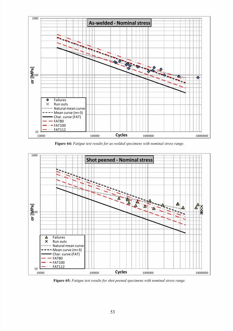
7/28/2019 Fulltext01 Chapter 4
http://slidepdf.com/reader/full/fulltext01-chapter-4 55/80
53
Figure 64: Fatigue test results for as-welded specimens with nominal stress range.
Figure 65: Fatigue test results for shot peened specimens with nominal stress range.
10
100
1000
10000 100000 1000000 10000000
σ r [ M P a ]
Cycles
As-welded - Nominal stress
FailuresRun outsNatural mean curveMean curve (m=3)
Char. curve (FAT)FAT80FAT100FAT112
10
100
1000
10000 100000 1000000 10000000
σ r [ M P a ]
Cycles
Shot peened - Nominal stress
FailuresRun outsNatural mean curveMean curve (m=3)Char. curve (FAT)FAT80FAT100FAT112
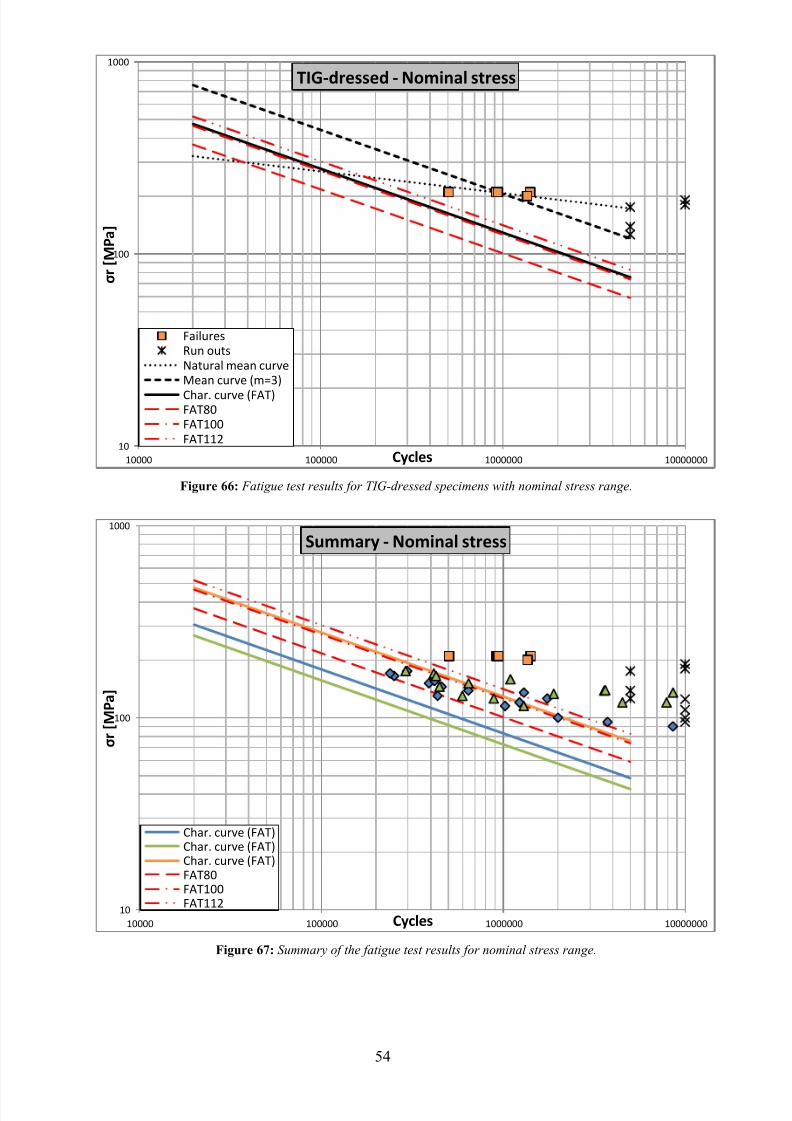
7/28/2019 Fulltext01 Chapter 4
http://slidepdf.com/reader/full/fulltext01-chapter-4 56/80
54
Figure 66: Fatigue test results for TIG-dressed specimens with nominal stress range.
Figure 67: Summary of the fatigue test results for nominal stress range.
10
100
1000
10000 100000 1000000 10000000
σ r [ M P a ]
Cycles
TIG-dressed - Nominal stress
FailuresRun outsNatural mean curveMean curve (m=3)
Char. curve (FAT)FAT80FAT100FAT112
10
100
1000
10000 100000 1000000 10000000
σ r [ M P a ]
Cycles
Summary - Nominal stress
Char. curve (FAT)Char. curve (FAT)Char. curve (FAT)FAT80FAT100FAT112
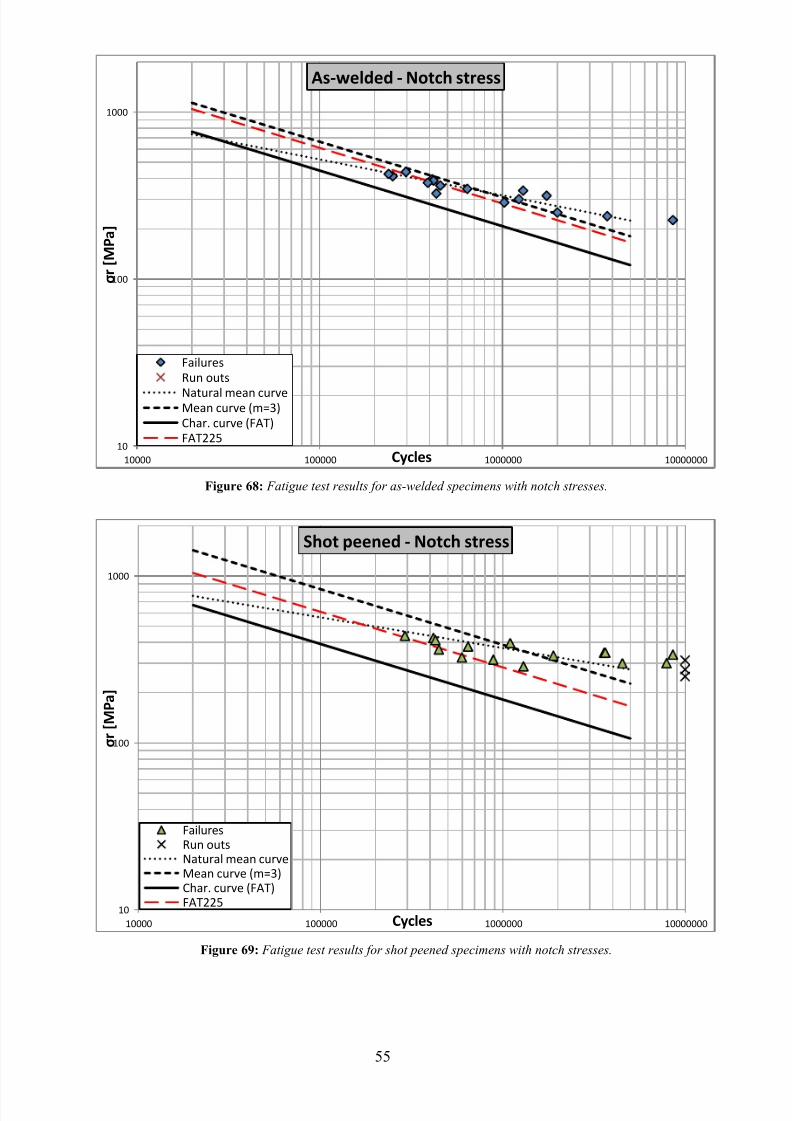
7/28/2019 Fulltext01 Chapter 4
http://slidepdf.com/reader/full/fulltext01-chapter-4 57/80
55
Figure 68: Fatigue test results for as-welded specimens with notch stresses.
Figure 69: Fatigue test results for shot peened specimens with notch stresses.
10
100
1000
10000 100000 1000000 10000000
σ r [ M P a ]
Cycles
As-welded - Notch stress
FailuresRun outs
Natural mean curveMean curve (m=3)Char. curve (FAT)FAT225
10
100
1000
10000 100000 1000000 10000000
σ r [ M P a ]
Cycles
Shot peened - Notch stress
FailuresRun outsNatural mean curveMean curve (m=3)Char. curve (FAT)FAT225
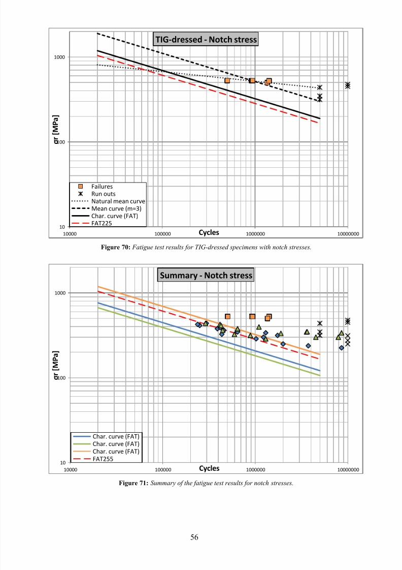
7/28/2019 Fulltext01 Chapter 4
http://slidepdf.com/reader/full/fulltext01-chapter-4 58/80
56
Figure 70: Fatigue test results for TIG-dressed specimens with notch stresses.
Figure 71: Summary of the fatigue test results for notch stresses.
10
100
1000
10000 100000 1000000 10000000
σ r [ M P a ]
Cycles
TIG-dressed - Notch stress
FailuresRun outs
Natural mean curveMean curve (m=3)Char. curve (FAT)FAT225
10
100
1000
10000 100000 1000000 10000000
σ r [ M P a ]
Cycles
Summary - Notch stress
Char. curve (FAT)Char. curve (FAT)Char. curve (FAT)FAT255
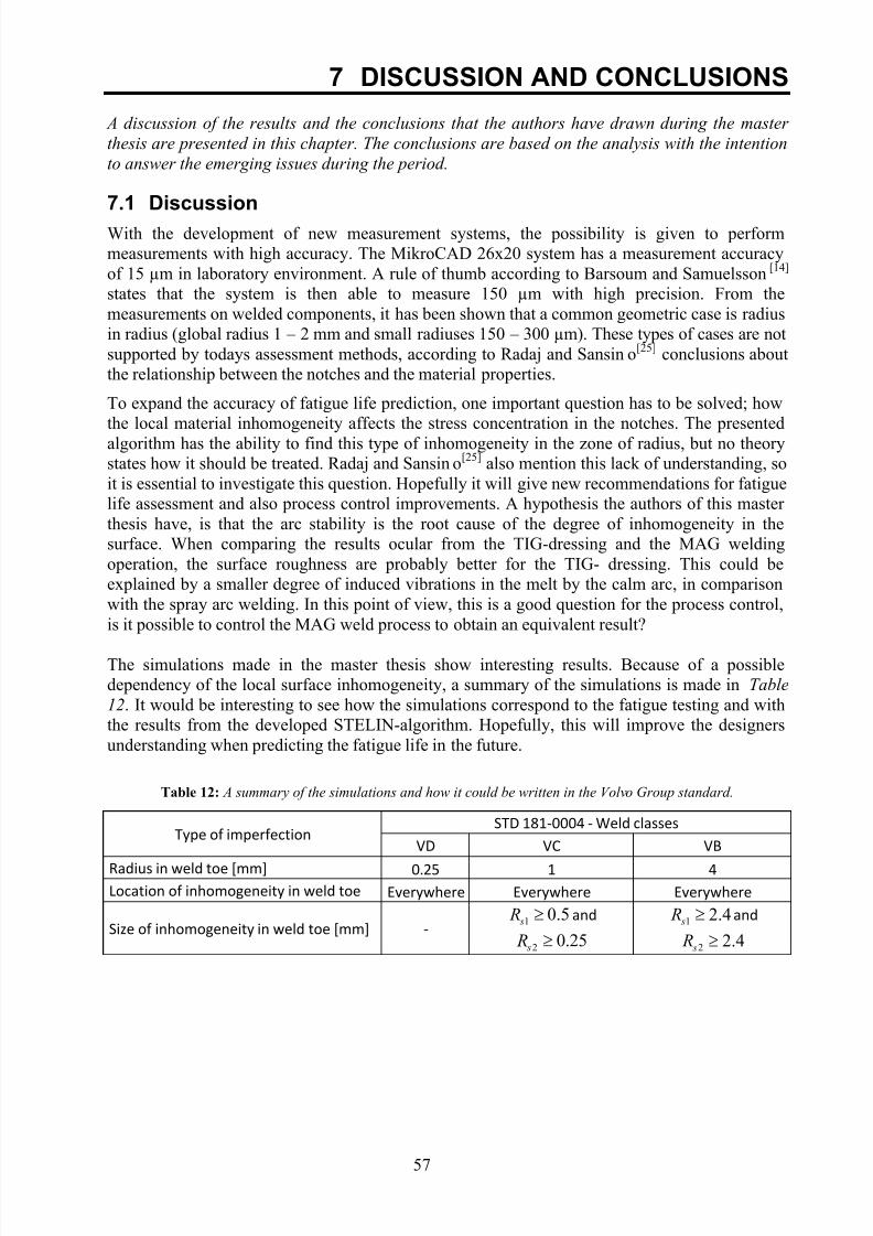
7/28/2019 Fulltext01 Chapter 4
http://slidepdf.com/reader/full/fulltext01-chapter-4 59/80
57
7 DISCUSSION AND CONCLUSIONS
A discussion of the results and the conclusions that the authors have drawn during the master
thesis are presented in this chapter. The conclusions are based on the analysis with the intention
to answer the emerging issues during the period.
7.1 Discussion
With the development of new measurement systems, the possibility is given to performmeasurements with high accuracy. The MikroCAD 26x20 system has a measurement accuracyof 15 µm in laboratory environment. A rule of thumb according to Barsoum and Samuelsson[14] states that the system is then able to measure 150 µm with high precision. From themeasurements on welded components, it has been shown that a common geometric case is radiusin radius (global radius 1 – 2 mm and small radiuses 150 – 300 µm). These types of cases are notsupported by todays assessment methods, according to Radaj and Sansino[25] conclusions aboutthe relationship between the notches and the material properties.
To expand the accuracy of fatigue life prediction, one important question has to be solved; howthe local material inhomogeneity affects the stress concentration in the notches. The presentedalgorithm has the ability to find this type of inhomogeneity in the zone of radius, but no theorystates how it should be treated. Radaj and Sansino[25] also mention this lack of understanding, soit is essential to investigate this question. Hopefully it will give new recommendations for fatiguelife assessment and also process control improvements. A hypothesis the authors of this master thesis have, is that the arc stability is the root cause of the degree of inhomogeneity in thesurface. When comparing the results ocular from the TIG-dressing and the MAG weldingoperation, the surface roughness are probably better for the TIG- dressing. This could beexplained by a smaller degree of induced vibrations in the melt by the calm arc, in comparisonwith the spray arc welding. In this point of view, this is a good question for the process control,is it possible to control the MAG weld process to obtain an equivalent result?
The simulations made in the master thesis show interesting results. Because of a possibledependency of the local surface inhomogeneity, a summary of the simulations is made in Table
12. It would be interesting to see how the simulations correspond to the fatigue testing and withthe results from the developed STELIN-algorithm. Hopefully, this will improve the designersunderstanding when predicting the fatigue life in the future.
Table 12: A summary of the simulations and how it could be written in the Volvo Group standard.
Type of imperfectionSTD 181-0004 - Weld classes
VD VC VB
Radius in weld toe [mm] 0.25 1 4Location of inhomogeneity in weld toe Everywhere Everywhere Everywhere
Size of inhomogeneity in weld toe [mm] -1 0.5 s R and
2 0.25 s R
1 2.4 s R and
2 2.4 s R
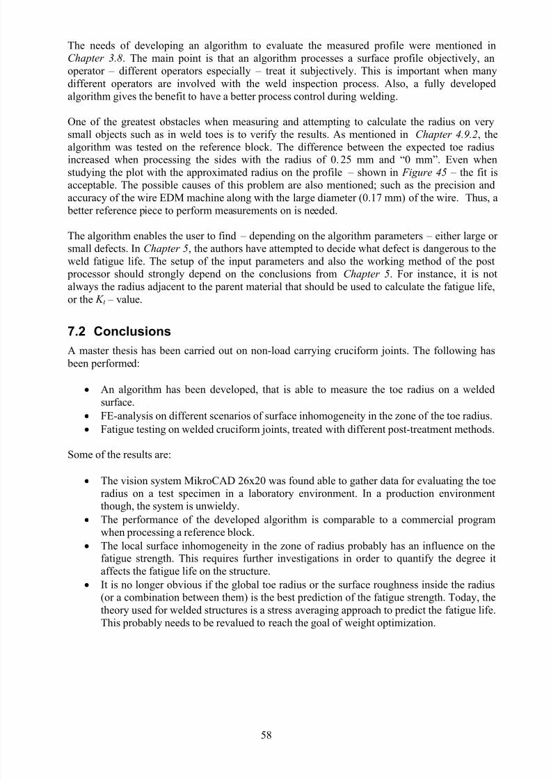
7/28/2019 Fulltext01 Chapter 4
http://slidepdf.com/reader/full/fulltext01-chapter-4 60/80
58
The needs of developing an algorithm to evaluate the measured profile were mentioned inChapter 3.8. The main point is that an algorithm processes a surface profile objectively, anoperator – different operators especially – treat it subjectively. This is important when manydifferent operators are involved with the weld inspection process. Also, a fully developedalgorithm gives the benefit to have a better process control during welding.
One of the greatest obstacles when measuring and attempting to calculate the radius on very
small objects such as in weld toes is to verify the results. As mentioned in Chapter 4.9.2, thealgorithm was tested on the reference block. The difference between the expected toe radiusincreased when processing the sides with the radius of 0.25 mm and “0 mm”. Even when
studying the plot with the approximated radius on the profile – shown in Figure 45 – the fit isacceptable. The possible causes of this problem are also mentioned; such as the precision andaccuracy of the wire EDM machine along with the large diameter (0.17 mm) of the wire. Thus, a
better reference piece to perform measurements on is needed.
The algorithm enables the user to find – depending on the algorithm parameters – either large or small defects. In Chapter 5, the authors have attempted to decide what defect is dangerous to theweld fatigue life. The setup of the input parameters and also the working method of the post
processor should strongly depend on the conclusions from Chapter 5. For instance, it is notalways the radius adjacent to the parent material that should be used to calculate the fatigue life,or the K t – value.
7.2 Conclusions
A master thesis has been carried out on non-load carrying cruciform joints. The following has been performed:
An algorithm has been developed, that is able to measure the toe radius on a weldedsurface.
FE-analysis on different scenarios of surface inhomogeneity in the zone of the toe radius. Fatigue testing on welded cruciform joints, treated with different post-treatment methods.
Some of the results are:
The vision system MikroCAD 26x20 was found able to gather data for evaluating the toeradius on a test specimen in a laboratory environment. In a production environmentthough, the system is unwieldy.
The performance of the developed algorithm is comparable to a commercial programwhen processing a reference block.
The local surface inhomogeneity in the zone of radius probably has an influence on thefatigue strength. This requires further investigations in order to quantify the degree itaffects the fatigue life on the structure.
It is no longer obvious if the global toe radius or the surface roughness inside the radius(or a combination between them) is the best prediction of the fatigue strength. Today, thetheory used for welded structures is a stress averaging approach to predict the fatigue life.This probably needs to be revalued to reach the goal of weight optimization.

7/28/2019 Fulltext01 Chapter 4
http://slidepdf.com/reader/full/fulltext01-chapter-4 61/80
59
8 RECOMMENDATIONS AND FUTURE WORK In this chapter, the recommendations on more detailed solutions and the future work are
presented.
8.1 Recommendations
Continue with performing simulations on welded joints and different cases of loading. Theresults will serve as a base when developing a post processor that evaluates the calculated radiialong the weld toe.
Investigate the crack surfaces to bring conclusions about the low FAT -values. This will alsomake it possible to see the relationship between the results given from the algorithm and thefatigue testing.
When the STELIN-algorithm is considered to perform as desired, start evaluating differentmeasurement systems that are designed and more appropriate in a production environment.
8.2 Future work
Improve the STELIN-algorithm by adding functions that calculates the toe angle and theweld throat size.
To predict the fatigue strength reduction, FE-simulations have to be done with fatiguetesting to see the relationship between measurements (of the toe radius) and the crack initiation point. This will hopefully provide a greater understanding of the toe radiusinfluence and stabilize the weld quality to reduce the scatter in fatigue life.
Validate the results from the performed FE- simulations with extended fatigue testing.This moment should also include studying of the fracture surfaces in order to determine
relationships between the crack initiation points and geometrical defects.
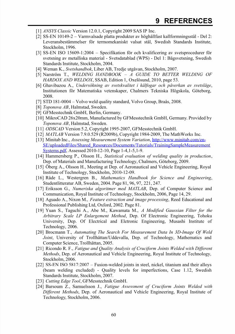
7/28/2019 Fulltext01 Chapter 4
http://slidepdf.com/reader/full/fulltext01-chapter-4 62/80
60
9 REFERENCES
[1] ANSYS Classic Version 12.0.1, Copyright 2009 SAS IP Inc.[2] SS-EN 10149-2 – Varmvalsade platta produkter av höghållfast kallformningsstål - Del 2:
Leveransbestämmelser för termomekaniskt valsat stål, Swedish Standards Institute,Stockholm, 1996.
[3] SS-EN ISO 15609-1:2004 – Specifikation för och kvalificering av svetsprocedurer för
svetsning av metalliska material - Svetsdatablad (WPS) - Del 1: Bågsvetsning, SwedishStandards Institute, Stockholm, 2004.
[4] Weman K., Svetshandbok , Liber AB, Tredje utgåvan, Stockholm, 2007.[5] Narström T., WELDING HANDBOOK – A GUIDE TO BETTER WELDING OF
HARDOX AND WELDOX , SSAB, Edition 1, Oxelösund, 2010, page 53.[6] Ghavibazou A., Undersökning av svetskvalitet i kälfogar och påverkan av svetsläge,
Institutionen för Matematiska vetenskaper, Chalmers Tekniska Högskola, Göteborg,2008.
[7] STD 181-0004 – Volvo weld quality standard, Volvo Group, Braås, 2008.[8] Toponova AB, Halmstad, Sweden.[9] GFMesstechnik GmbH, Berlin, Germany.
[10] MikroCAD 26x20mm, Manufactured by GFMesstechnik GmbH, Germany. Provided byToponova AB, Halmstad, Sweden.
[11] ODSCAD Version 5.2, Copyright 1995-2007, GFMesstechnik GmbH. [12] MATLAB Version 7.9.0.529 (R2009b), Copyright 1984-2009, The MathWorks Inc.[13] Minitab Inc., Assessing Measurement System Variation, http://www.minitab.com/en-
SE/uploadedFiles/Shared_Resources/Documents/Tutorials/TrainingSampleMeasurementSystems.pdf , Assessed 2010-12-10, Page 1-4,1-5,1-9.
[14] Hammersberg P., Olsson H., Statistical evaluation of welding quality in production,Dep. of Materials and Manufacturing Technology, Chalmers, Göteborg, 2009.
[15] Öberg A., Olsson H., Meeting at Dep. of Aeronautical and Vehicle Engineering, RoyalInstitute of Technology, Stockholm, 2010-12-09.
[16] Råde L., Westergren B., Mathematics Handbook for Science and Engineering ,Studentlitteratur AB, Sweden, 2004. Page 81, 96, 97, 221, 247.
[17] Eriksson G., Numeriska algoritmer med MATLAB, Dep. of Computer Science andCommunication, Royal Institute of Technology, Stockholm, 2006, Page 14, 29.
[18] Aguado A., Nixon M., Feature extraction and image processing , Reed Educational andProfessional Publishing Ltd, Oxford, 2002. Page 81.
[19] Yuan S., Taguchi A., Abe M., Kawamata M., A Modified Gaussian Filter for the
Arbitrary Scale LP Enlargement Method , Dep. Of Electronic Engineering, TohokuUniversity, Dep. Of Electrical and Eletronic Engineering, Musashi Institute of Technology, 2006.
[20] Brocmann T., Automating The Search For Measurement Data In 3D-Image Of Weld Joint , University of Trollhättan/Uddevalla, Dep. of Technology, Mathematics andComputer Science, Trollhättan, 2005.
[21] Ricondo R. F., Fatigue and Quality Analysis of Cruciform Joints Welded with Different
Methods, Dep. of Aeronautical and Vehicle Engineering, Royal Institute of Technology,Stockholm, 2006.
[22] SS-EN ISO 5817:2007 – Fusion-welded joints in steel, nickel, titanium and their alloys(beam welding excluded) - Quality levels for imperfections, Case 1.12, SwedishStandards Institute, Stockholm, 2007.
[23] Cutting Edge Tool , GFMesstechnik GmbH.[24] Barsoum Z., Samuelsson J., Fatigue Assessment of Cruciform Joints Welded with
Different Methods, Dep. of Aeronautical and Vehicle Engineering, Royal Institute of Technology, Stockholm, 2006.

7/28/2019 Fulltext01 Chapter 4
http://slidepdf.com/reader/full/fulltext01-chapter-4 63/80
61
[25] Radaj D., Sonsino C. M., Fatigue Assessment of Welded Joints by Local Approaches,Abington Publishing, England, 1998.
[26] Barsoum Z., Fatigue design methods for welded joints, Presentationsmaterial, SD2420Avancerad dimensionering av svetsade konstruktioner, Kungliga Tekniska Högskolan,Stockholm, 2009.
[27] Hobbacher A., “ Fatigue design of welded joints and components”, IIW doc. XIII-1539-96, 1996.
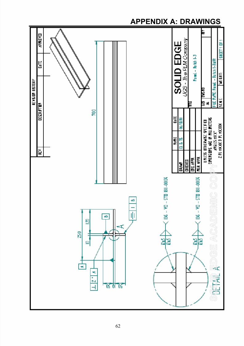
7/28/2019 Fulltext01 Chapter 4
http://slidepdf.com/reader/full/fulltext01-chapter-4 64/80
62
APPENDIX A: DRAWINGS
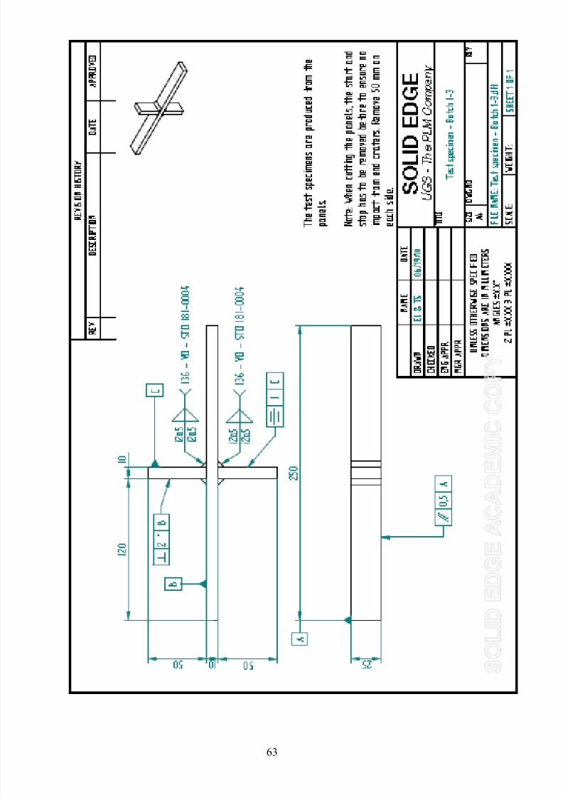
7/28/2019 Fulltext01 Chapter 4
http://slidepdf.com/reader/full/fulltext01-chapter-4 65/80
63
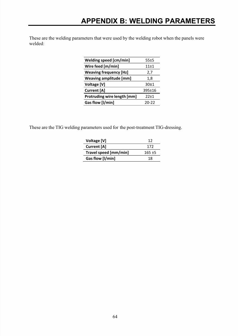
7/28/2019 Fulltext01 Chapter 4
http://slidepdf.com/reader/full/fulltext01-chapter-4 66/80
64
APPENDIX B: WELDING PARAMETERS
These are the welding parameters that were used by the welding robot when the panels werewelded:
Welding speed [cm/min] 55±5
Wire feed [m/min] 11±1
Weaving frequency [Hz] 2,7
Weaving amplitude [mm] 1,8
Voltage [V] 30±1
Current [A] 395±16
Protruding wire length [mm] 22±1
Gas flow [l/min] 20-22
These are the TIG welding parameters used for the post-treatment TIG-dressing.
Voltage [V] 12
Current [A] 172
Travel speed [mm/min] 165 ±5
Gas flow [l/min] 18
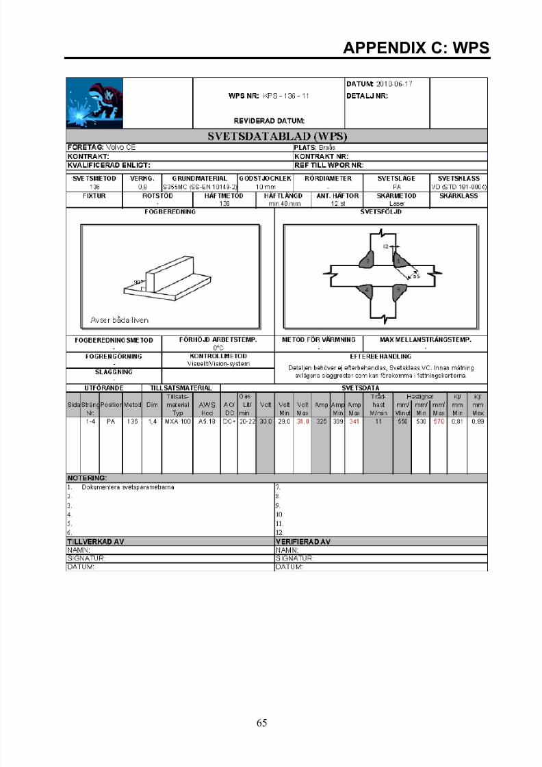
7/28/2019 Fulltext01 Chapter 4
http://slidepdf.com/reader/full/fulltext01-chapter-4 67/80
65
APPENDIX C: WPS
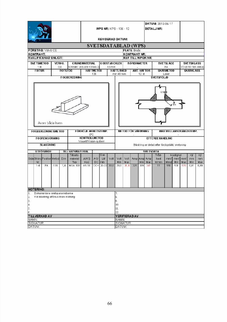
7/28/2019 Fulltext01 Chapter 4
http://slidepdf.com/reader/full/fulltext01-chapter-4 68/80
66
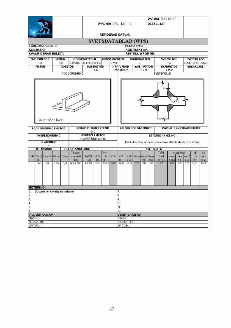
7/28/2019 Fulltext01 Chapter 4
http://slidepdf.com/reader/full/fulltext01-chapter-4 69/80
67
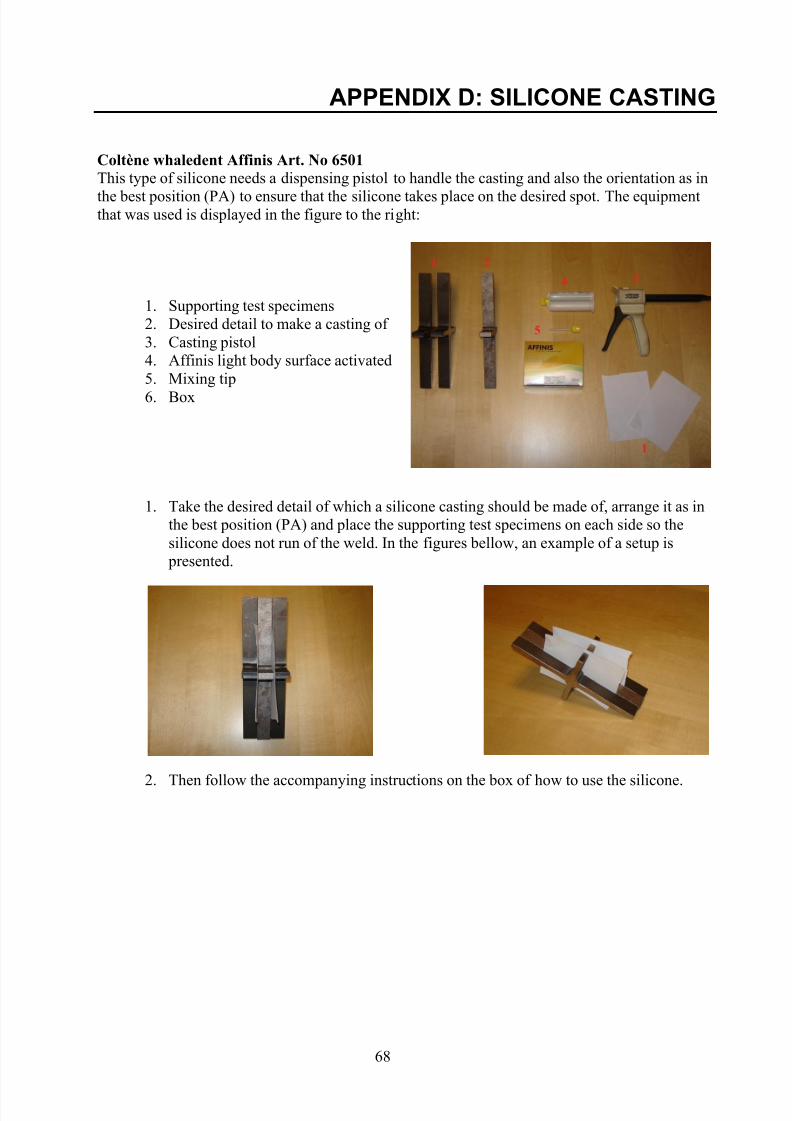
7/28/2019 Fulltext01 Chapter 4
http://slidepdf.com/reader/full/fulltext01-chapter-4 70/80
68
APPENDIX D: SILICONE CASTING
Coltène whaledent Affinis Art. No 6501
This type of silicone needs a dispensing pistol to handle the casting and also the orientation as in
the best position (PA) to ensure that the silicone takes place on the desired spot. The equipmentthat was used is displayed in the figure to the right:
1. Supporting test specimens2. Desired detail to make a casting of 3. Casting pistol4. Affinis light body surface activated5. Mixing tip
6. Box
1. Take the desired detail of which a silicone casting should be made of, arrange it as inthe best position (PA) and place the supporting test specimens on each side so thesilicone does not run of the weld. In the figures bellow, an example of a setup is
presented.
2. Then follow the accompanying instructions on the box of how to use the silicone.

7/28/2019 Fulltext01 Chapter 4
http://slidepdf.com/reader/full/fulltext01-chapter-4 71/80
69
3. Mount the pistol with the silicone container and apply it on the weld, try to get auniform distribution of the silicone.
4. After applying the silicone, it should temper for at least 10 minutes. It is a bit over therecommended time because of the difference in the environment that is described inthe instructions.
5. When these 10 minutes have passed, the casting process is finished.
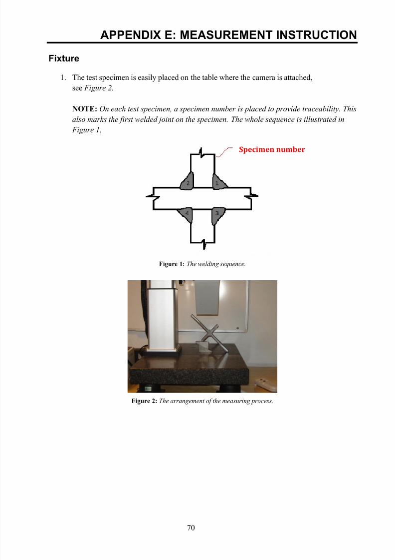
7/28/2019 Fulltext01 Chapter 4
http://slidepdf.com/reader/full/fulltext01-chapter-4 72/80
70
APPENDIX E: MEASUREMENT INSTRUCTION
Fixture
1. The test specimen is easily placed on the table where the camera is attached,
see Figure 2.
NOTE: On each test specimen, a specimen number is placed to provide traceability. This
also marks the first welded joint on the specimen. The whole sequence is illustrated in
Figure 1.
Figure 1: The welding sequence.
Figure 2: The arrangement of the measuring process.
Specimen number
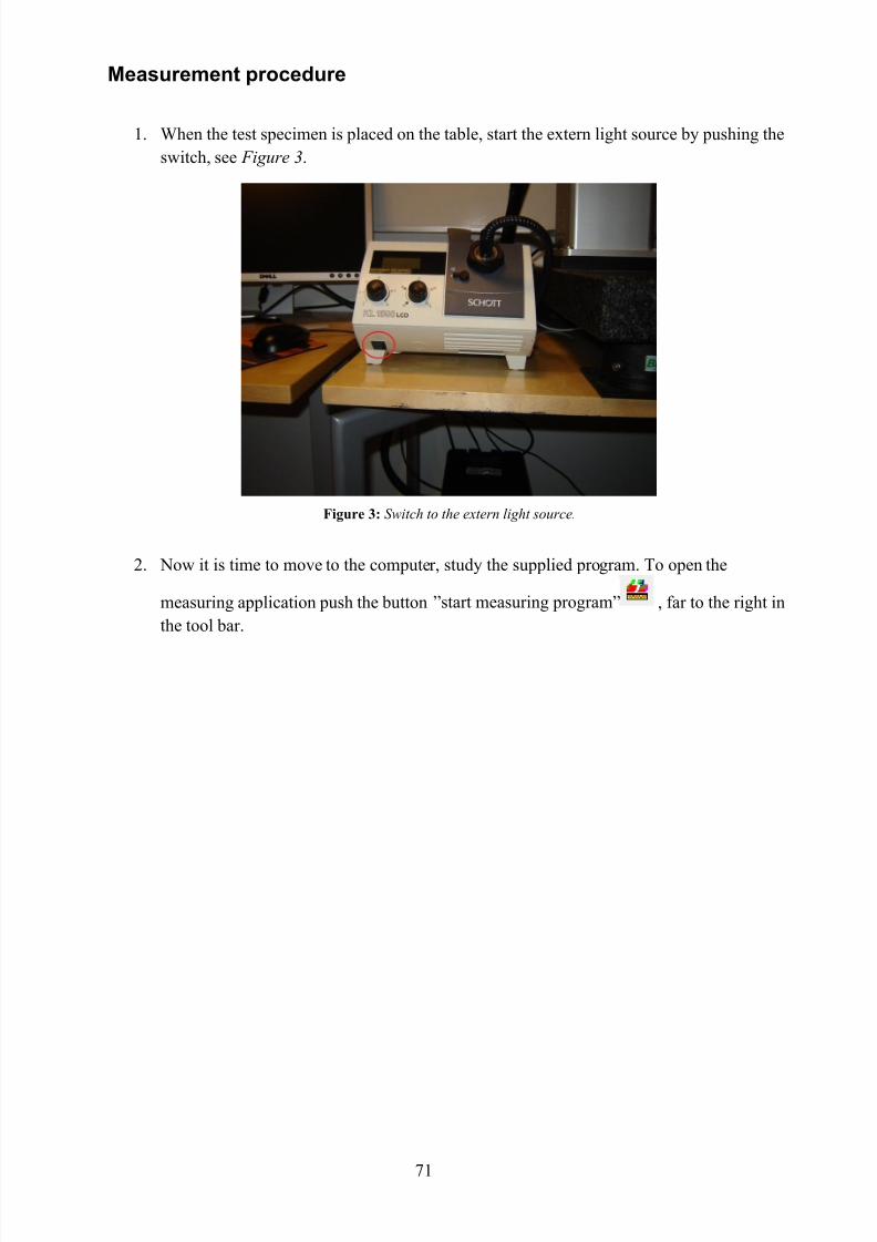
7/28/2019 Fulltext01 Chapter 4
http://slidepdf.com/reader/full/fulltext01-chapter-4 73/80
71
Measurement procedure
1. When the test specimen is placed on the table, start the extern light source by pushing the
switch, see Figure 3.
Figure 3: Switch to the extern light source.
2. Now it is time to move to the computer, study the supplied program. To open the
measuring application push the button ”start measuring program” , far to the right in
the tool bar.

7/28/2019 Fulltext01 Chapter 4
http://slidepdf.com/reader/full/fulltext01-chapter-4 74/80
72
3. a. To find the correct focus height in the measuring system, use the controller to
make a rough calibration and the adjustment knob on the left to make a finer
calibration, see Figure 4.
b. On the computer screen it is now possible to see a red cross with a black
background, see Figure 5. By moving the camera tripod downward, the focus will
change and a clearer view will be shown of the specimen on the screen.c. It will also appear a projected light of a black cross with four squares when the
correct focus approaches, these should be fitted in the red cross on the highest
point on the weld bead, see Figure 6 .
Figure 4: The controller to move the camera up and down.
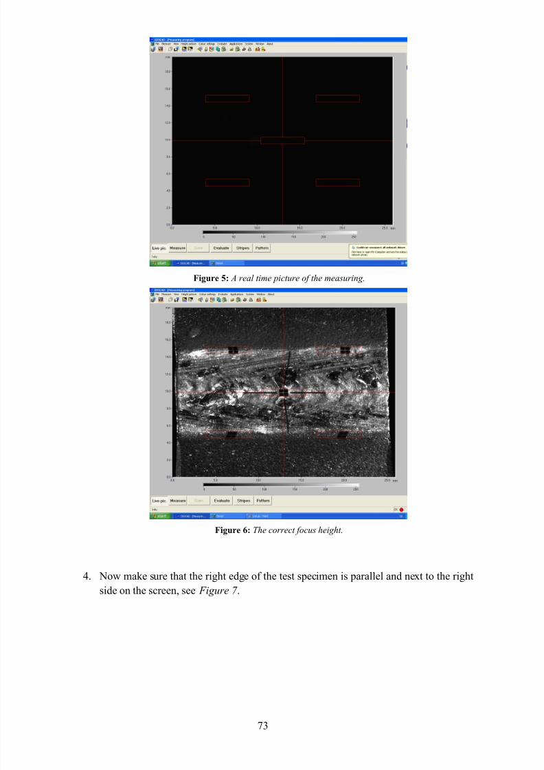
7/28/2019 Fulltext01 Chapter 4
http://slidepdf.com/reader/full/fulltext01-chapter-4 75/80
73
Figure 5: A real time picture of the measuring.
Figure 6: The correct focus height.
4. Now make sure that the right edge of the test specimen is parallel and next to the right
side on the screen, see Figure 7 .
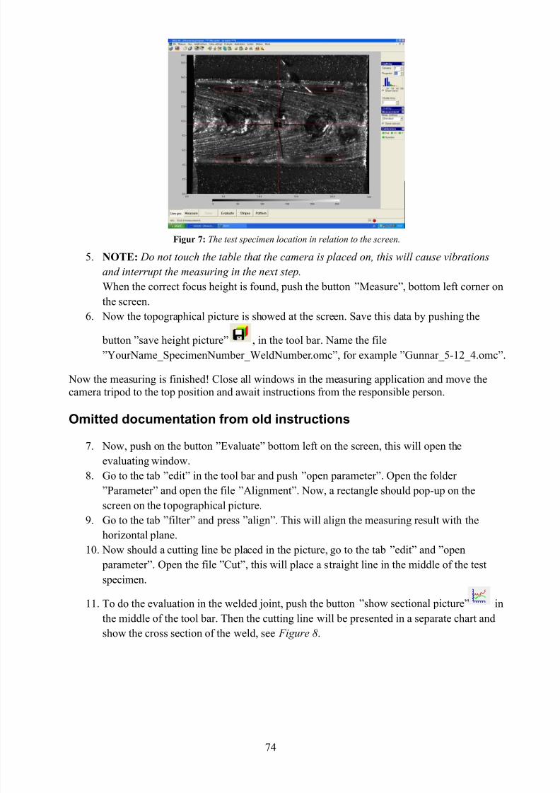
7/28/2019 Fulltext01 Chapter 4
http://slidepdf.com/reader/full/fulltext01-chapter-4 76/80
74
Figur 7: The test specimen location in relation to the screen.
5. NOTE: Do not touch the table that the camera is placed on, this will cause vibrations
and interrupt the measuring in the next step.
When the correct focus height is found, push the button ”Measure”, bottom left corner on
the screen.
6. Now the topographical picture is showed at the screen. Save this data by pushing the
button ”save height picture” , in the tool bar. Name the file
”YourName_SpecimenNumber_WeldNumber .omc”, for example ”Gunnar_5-12_4.omc”.
Now the measuring is finished! Close all windows in the measuring application and move thecamera tripod to the top position and await instructions from the responsible person.
Omitted documentation from old instructions
7. Now, push on the button ”Evaluate” bottom left on the screen, this will open the
evaluating window.
8. Go to the tab ”edit” in the tool bar and push ”open parameter”. Open the folder
”Parameter” and open the file ”Alignment”. Now, a rectangle should pop-up on the
screen on the topographical picture.
9. Go to the tab ”filter” and press ”align”. This will align the measuring result with the
horizontal plane.
10. Now should a cutting line be placed in the picture, go to the tab ”edit” and ”open
parameter”. Open the file ”Cut”, this will place a straight line in the middle of the test
specimen.
11. To do the evaluation in the welded joint, push the button ”show sectional picture” in
the middle of the tool bar. Then the cutting line will be presented in a separate chart and
show the cross section of the weld, see Figure 8.

7/28/2019 Fulltext01 Chapter 4
http://slidepdf.com/reader/full/fulltext01-chapter-4 77/80
75
Figure 8: A cross section of the weld.
12. To give the same scaling of the axis, go to the tab ”View” and push on ”Real XY ratio”.
The evaluation is going to be performed in two different steps, the first in a non-zoomed viewand the second in a zoomed view of 2 * 1 mm.
Non-zoomed view
The interesting toe radius, in this case, is the left one in Figure 8, because it is the toe that thestress will pass by for a non-load carrying cruciform welded joint.
1. Now the operator shall do an assessment where he or she thinks the radius starts and
stops. When he or she has decided where, place two points by left-click with the mouse
over the area.
2. Write the x- and y-coordinates for the start and end point on a paper, this will be used
over again.
3. Now the operator should evenly distribute three points inside the start and end point.
4. To calculate the radius push the button ”Radius” in the tool bar.
5. Do a print screen of the radius by pushing the button ”Print Screen”, up to the right on the
keyboard. Switch to the program ”Paint” and push ”ctrl + v” to paste the picture. Save as
”YourNamn_SpecimenNumber_WeldNumber_RadiusNumber .png”.
6. Inform the responsible person to write down the obtained radius.7. Right click on the radius with the mouse to erase it.
8. Now, perform the same procedure one more time, but distribute 7 points inside the start
and end point instead of 3 points. Once again the responsible person should be informed
to write down the obtained radius.
9. Right click on the radius with the mouse to erase it.
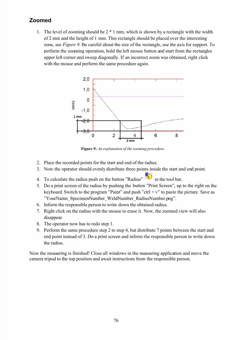
7/28/2019 Fulltext01 Chapter 4
http://slidepdf.com/reader/full/fulltext01-chapter-4 78/80
76
Zoomed
1. The level of zooming should be 2 * 1 mm, which is shown by a rectangle with the width
of 2 mm and the height of 1 mm. This rectangle should be placed over the interesting
zone, see Figure 9. Be careful about the size of the rectangle, use the axis for support. To
perform the zooming operation, hold the left mouse button and start from the rectangles
upper left corner and sweep diagonally. If an incorrect zoom was obtained, right click with the mouse and perform the same procedure again.
Figure 9: An explanation of the zooming procedure.
2. Place the recorded points for the start and end of the radius.
3. Now the operator should evenly distribute three points inside the start and end point.
4. To calculate the radius push on the button ”Radius” in the tool bar.5. Do a print screen of the radius by pushing the button ”Print Screen”, up to the right on the
keyboard. Switch to the program ”Paint” and push ”ctrl + v” to paste the picture. Save as
”YourNamn_ Specimen Number_WeldNumber_RadiusNumber.png”.
6. Inform the responsible person to write down the obtained radius.
7. Right click on the radius with the mouse to erase it. Now, the zoomed view will also
disappear.
8. The operator now has to redo step 1.
9. Perform the same procedure step 2 to step 4, but distribute 7 points between the start and
end point instead of 3. Do a print screen and inform the responsible person to write downthe radius.
Now the measuring is finished! Close all windows in the measuring application and move thecamera tripod to the top position and await instructions from the responsible person.
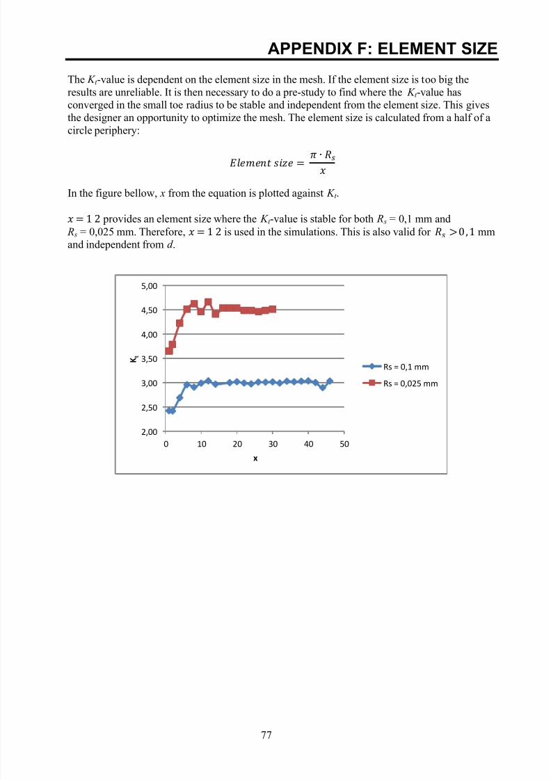
7/28/2019 Fulltext01 Chapter 4
http://slidepdf.com/reader/full/fulltext01-chapter-4 79/80
77
APPENDIX F: ELEMENT SIZE
The K t -value is dependent on the element size in the mesh. If the element size is too big theresults are unreliable. It is then necessary to do a pre-study to find where the K t -value hasconverged in the small toe radius to be stable and independent from the element size. This givesthe designer an opportunity to optimize the mesh. The element size is calculated from a half of acircle periphery:
In the figure bellow, x from the equation is plotted against K t .
provides an element size where the K t -value is stable for both R s = 0,1 mm and R s = 0,025 mm. Therefore, is used in the simulations. This is also valid for mmand independent from d .
2,00
2,50
3,00
3,50
4,00
4,50
5,00
0 10 20 30 40 50
K t
x
Rs = 0,1 mm
Rs = 0,025 mm
7/28/2019 Fulltext01 Chapter 4
http://slidepdf.com/reader/full/fulltext01-chapter-4 80/80

![The Capital Asset Pricing Model - DiVA portal139114/FULLTEXT01.pdf · ... 18 4. METHODOLOGY ... the conclusions in Chapter 6. 1 Brealey, Myers, Allen [2006] ... The Capital Asset](https://img.dokumen.tips/doc/110x75/5ae118767f8b9a6e5c8e4617/the-capital-asset-pricing-model-diva-139114fulltext01pdf-18-4-methodology.jpg)