Embed Size (px)
Citation preview
Full Characterization of a Strange Attractor
Chaotic Dynamics in Low-dimensional Replicator Systems
By
Wolfgang Schnabl, Peter F.Stadler, Christian Forst
and Peter Schuster ∗
Institut fur theoretische Chemie der Universitat Wien
Mailing Address: Prof.Peter Schuster, Institut fur theoretische Chemie
der Universitat Wien
Wahringerstraße 17, A 1090 Wien, Austria
Phone: (0222) 43 61 41 / 78 D
Bitnet: A8441DAM@AWIUNI11
W.Schnabl et al.: Chaotic Attractor Page 1
Abstract
Two chaotic attractors observed in Lotka-Volterra equations of dimension
n = 3 are shown to represent two different cross-sections of one and the same
chaotic regime. The strange attractor is studied in the equivalent four dimen-
sional catalytic replicator network. Analytical expression are derived for the
Ljapunov exponents of the flow. In the centre of the chaotic regime the strange
attractor is characterized by numerically computated Renyi fractal dimensions,
Dq (q = 0, 1, 2) = 2.04, 1.89 and 1.65 ± 0.05 as well as the Ljapunov dimension
DL = 2.06 ± 0.02. Accordingly it represents a multifractal . The fractal set is
characterized by the singularity spectrum.
Two routes in parameter space leading into the chaotic regime were studied in
detail, one corresponding to the Feigenbaum cascade of bifurcations. The second
route is substantial different from this well known pathway and has some features
in common with the intermittency route. A series of one-dimensional maps is
derived from a properly chosen Poincare cross-section which illustrates structural
changes in the attractor.
Mutations are included in the catalytic replicator network and the changes in
the dynamics observed are compared with the predictions of an approach based
on pertubation theory. The most striking result is the gradual disappearance of
complex dynamics with increasing mutation rates.
W.Schnabl et al.: Chaotic Attractor Page 2
1. Introduction
The search for chaotic dynamics became an issue in many scientific disciplines
from physics to biology. The relevance of strange attractors in modeling real sys-
tems and the problem how to trace chaos in the experimental data were important
questions already five years ago [1] and remained in the centre of interest since
then [2-4] . Numerical evidence for strange attractors was found in many model
equations but unlike simple attractors they cannot be characterized by a few coor-
dinates or coordinates and frequencies. In the poineering works of several groups
efficient techniques to analyse chaotic dynamics and fractal sets were developed
(For a recent review of the available repertoire of methods see [5,6]). In order
to provide a sufficiently detailed basis for the comparison of model calculations
and experimental data full characterization of strange attractors is required. We
present such a study on a chaotic attractor which appears in the solutions of a
differential equation which is of interest in biophysics and in theoretical ecology
as well as in other disciplines.
Autocatalytic reaction networks which involve two classes of catalytic pro-
cesses – autocatalytic instruction for reproduction as well as material and process
specific catalysis – were postulated as models for studies on prebiotic and early bio-
logical evolution scenarios [7,8]. Now they serve also as simple models showing the
characteristic features of nonlinear dynamics in very different fields like molecular
biology, population genetics, theoretical ecology or dynamical game theory [9] .
Qualitative analysis and systematic numerical investigations revealed a very
rich dynamics of the corresponding kinetic differential equations [10] . The name
W.Schnabl et al.: Chaotic Attractor Page 3
replicator equations was coined for these systems because they reveal several
unique and – in the standardized form to be discussed in the next section 2 –
fairly easy to proof features [11] . The four species replicator system shows chaotic
dynamics for certain parameter values [12] . According to Hofbauer [13] this au-
tocatalytic network with four species is – apart from a transformation of the time
scale – equivalent to a three-species Lotka-Volterra equation. Possible existence
of very complex dynamical behaviour in Lotka-Volterra models was predicted by
Smale [14] . Indeed two different strange attractors were reported for the Lotka-
Volterra system [15-18], which describes communities of one predator species
living on two prey species. In this contribution we shall show that the two strange
attractors lie on different cross-sections through one and the same chaotic regime.
The number of degrees of freedom is minimal for the occurrence of strange at-
tractors and hence the chaotic regime in question houses the simplest strange
attractors possible in Lotka-Volterra and replicator equations – replicator systems
have normalized variables and hence the number of independent degrees of freedom
is the number of species but one.
2.The replicator model
Replicator equations are based on the simplest possible molecular mechanism
of catalysed replication and mutation. The basic reactions are of the form
(A) + Ij + Ii
Qkj ·Aji
−−−→ Ij + Ik + Ii ; i, j, k = 1, . . . , n . (1)
W.Schnabl et al.: Chaotic Attractor Page 4
Herein Ij is the template which is replicated and Ii the catalyst, (A) represents
an overall notation for substrates needed for replication. It is assumed that the
substrates are present in excess – their concentration are buffered and hence do
not change during the course of reactions. There are n3 possible reactions produc-
ing the n different species Ik(k = 1, . . . , n) of the autocatalytic reaction network.
Clearly it is very hard – if not impossible – to handle such a large number of param-
eters. In order to be able to analyse the reaction network simplifying assumptions
are inevitable. It is straight forward to treat catalysed replication and mutation
as independent superpositions: mutation frequencies depend on template (Ij) and
target (Ik), but not on the catalyst (Ii). The remaining 2n2 rate parameters are
properly understood then as elements of two n × n matrices: a replication rate
matrix A.= (Aji) and a mutation matrix Q
.= (Qkj). The rate constants of the
individual reactions are products of a replication and a mutation factor. Qkj ·Aji,
expressing the following sequence of processes: Ii catalyzes the replication of Ij
which yields Ik as an error copy .
Error-free replication of species Ij – described by equ.(1) with Ik ≡ Ij – is
assumed to occur with frequency Qjj . A mutation from Ij to Ik, (k 6= j) occurs
with frequency Qkj . Every copy has to be either correct or a mutant and thus Q
is a stochastic matrix (∑n
k=1 Qkj = 1 ∀ j = 1, . . . , n).
Concentrations of individual species are denoted by ck = [Ik]. As variables we
use relative – or normalized – concentrations: xk = ck
/
∑nj=1 cj which obviously
fulfil∑n
k=1 xk = 1.
W.Schnabl et al.: Chaotic Attractor Page 5
Mass action kinetics applied to the autocatalytic reaction-mutation network
(1) yields an ODE of the form
dxk
dt= xk =
n∑
i,j=1
QkiAijxixj − xkΦ, k = 1, . . . n (2)
where an automatically adjusted dilution flux
Φ =
n∑
i,j=1
Aijxixj
is introduced in order to keep the sum of relative concentrations normalized to
unity. The physically meaningful domain of equ.(2) is the simplex
Sn.=
{
(x1, . . . , xn) | xi ≥ 0,
n∑
i=1
xi = 1
}
If Aij ≥ 0, i, j = 1, . . . n then Sn is a compact, foreward invariant set for the
ODE (2).
An intensity of mutation can be measured by the mean mutation rate ε:
ε.=
1
n(n − 1)
n∑
i6=ji,j=1
Qij (3)
Throughout this paper we use a particularly simple type of the mutation matrix
Qij =
{
1 − (n − 1)ε, if i = j ;
ε, if i 6= j .
It represents a special case of the house of cards model of mutation [19,20] fre-
quently used in theoretical population genetics.
W.Schnabl et al.: Chaotic Attractor Page 6
The important special case of error-free replication is represented by a unit
mutation matrix, Q = id. Then equ.(1) is turned into the well known replicator
equation:
xk = xk
( n∑
i=1
Akixi −n
∑
i,j=1
Aijxixj
)
(4)
The linear replicator equation (4) for n is flow-equivalent to the n − 1 species
Lotka-Volterra equation:
yk = yk
(
αk +n−1∑
i=1
βkjyj
)
; k = 1, . . . , n − 1 . (5)
The variables are related by means of the transformation introduced by Hofbauer
[13]:
yk =xk
xn
for k = 1, . . . , n − 1 . (6)
3.The chaotic regime in parameter space
Two distinct chaotic attractors were found in Lotka-Volterra equations for
three species: Vance [17] discovered a “quasi-cyclic” trajectory in a one predator
two prey model and Arneodo, Coullet and Tresser [15] found a one parameter
family of strange attractors (ACT-attractor). We used Hofbauer’s transform to
construct the replicator equations which are equivalent to the models mentioned
above. Then a barycentric transform [21] was applied to Vance’s model in order
to shift the interior fixed point into the centre of the simplex S4 – the point
c = 14(1, 1, 1, 1).
W.Schnabl et al.: Chaotic Attractor Page 7
A barycentric transformation can always be found if the replicator equation
zk = zk
( n∑
i=1
bkizi −
n∑
i,j=1
bijzizj
)
has an interior fixed point z = (z1, z2, . . . , zn). It can be shown [22] that there
exists a diffeomorphism which relates this replicator equation to another one in
the notation of equ.(4) with
Aij =bij
zj
and x =1
n
(
1, 1, . . . , 1)
.
Both the ACT family and the Vance attractor (V) correspond to nonrobust
phase-portraits because of zero or almost zero (see e.g. A24 or A43 in AV ) off-
diagonal elements in the reaction matrices A. In order to make the numerical
computations easy to reproduce all parameter values were rounded to three digits.
Then the Vance model has a replication matrix
AV =
0 0.063 0 0.4370.537 0 −0.036 −0.001−0.535 0.38 0 0.6550.536 −0.032 −0.004 0
(7)
and the ACT attractors are found at
AACT =
0 0.5 −0.1 0.11.1 0 −0.6 0−0.5 1 0 0
1.7 + µ −1 − µ −0.2 0
(8)
Note that we use a parameter µ which corresponds to µ − 1.5 in [15].
In order to find out whether or not these two attractors are related in the
twelve-dimensional parameter space we performed a systematic numerical survey
W.Schnabl et al.: Chaotic Attractor Page 8
in the two-dimensional subspace (µ, ν) which connects the two models:
A(µ, ν) =
=
0 0.5 − 0.437ν −0.1 + 0.1ν 0.1 + 0.337ν
1.1 − 0.563ν 0 −0.6 + 0.564ν −0.001ν
−0.5 − 0.035ν 1 − 0.62ν 0 0.655ν
1.7 + µ − 1.164ν −1 − µ + 0.968ν −0.2 + 0.196ν 0
(9)
We note that all three matrices of replication constants fulfil∑4
j=1 Aij = 0.5 –
a property which will be used together with the existence of a fixed point in the
centre of the simplex later on.
In the (µ, ν)-plane the ACT model lies on the line −0.2 ≤ µ ≤ 0.05 and
ν = 0. The Vance-attractor is close to the point (0, 1). Both models are embedded
in a Σ-shaped two-dimensional manifold of strange attractors (fig.1). In scanning
through the manifold we could not find any sudden changes in the shape of the
attractor. The mean revolution time also varies in apparently continuous manner
all over the chaotic regime.
Fig. 1: A two-dimensional cross-section through the chaotic regime of
equ.(4). The cross-section is defined by the two parameters µ
and ν in the replication matrix A (9).
A common feature of all phase portraits exhibiting chaotic behaviour (attrac-
tive or only transient) is a saddle focus P123 on the [1, 2, 3]-plane, which represents
the stable manifold. The unstable manifold thus points into the interior of the
simplex. We found that Silnikov’s condition [23] is always satisfied: the real pos-
itive eigenvalue is larger in magnitude than the real parts of the two complex

W.Schnabl et al.: Chaotic Attractor Page 9
conjugate eigenvalues. Although there is no homoclinic orbit possible for P123, a
close relation to Silnikov’s condition is evident, as was pointed out by Arneodo
et al. [16]: there is a heteroclinic orbit involving three saddles instead of one and
this orbit replaces the homoclinic one. For generalized Lotka-Volterra models with
additional cubic terms Samardzija and Greller [24] found a different type of chaos
arising from a fractal torus.
For small values of µ the fixed point in the centre of S4 (c) is stable. Chaos
is reached via a Hopf bifurcation and a subsequent cascade of period doubling
bifurcations. At first the limit cycle, and then the chaotic attractor, both grow
steadily with increasing µ-values. At a parameter value around µ = 0.21 the
chaotic attractor collides with the stable manifold of a saddle on the [1, 2, 4]-plane
and disappears suddenly. This behaviour is known as limit crisis [25] : at the
bifurcation point we find a heteroclinic orbit connecting the [1, 4]-saddle, a saddle
on the [1, 2]-edge, and the saddle-focus in the [1, 2, 3]-plane (fig.2). The evidence for
the orbit is derived from numerical integration. We cannot provide an analytical
proof for the saddle connection between the saddle focus and P12. The saddle
connections on the boundary follow from the invariance of the subsimplices and
the classification of the flow of three component replicator equations [26,27].
Beyond the limit crisis we find a field of transient chaos: the trajectory seems
to draw an image of the chaotic attractor which in parameter space lies on the
other side of the limit crisis before it ends up in a stable fixed point.
For small values of ν the frequency of the oscillations increases with decreasing
parameter values – revolution times become shorter and shorter. Eventually the
W.Schnabl et al.: Chaotic Attractor Page 10
attractor collides with the stable manifold of the saddle on the [1, 2]-edge. The in-
variant hyperplane∑4
k=1 xk = 1 is a repellor in this area and therefore integration
is extremely sensitive to numerical errors.
Fig. 2: A sketch of fourteen flows on the boundaries of the simplex S4
which can coexist with the chaotic attractor in the interior. The
numbers (1) to (14) are used as markers in fig.1 to indicate where
the phase portraits occur in parameter space.
The chaotic attractor in the interior of the simplex S4 coexists with a rather
large variety of robust flows on the surface. Fig.2 shows fourteen boundary-flows
consistent with chaos on the (µ, ν)-plane.
Fig.3 sketches the phase portraits of the ACT and the Vance model together
with a typical chaotic trajectory for each system.
Fig. 3: Phase portraits and chaotic trajectories in the Vance (7) and the
ACT model (8).
Direct evidence from the inspection of computed trajectories was supple-
mented by Fourier transformation [28] . Some typical examples of Fourier spectra
in periodic and chaotic regimes of our attractor are shown in fig.4. They are used
as a sensitive indicator of the occurence of chaos. In the four spectra chosen we ob-
serve a complete transition from a periodic window into the chaotic regime caused
by a small change in the parameters (∆µ<0.02).

W.Schnabl et al.: Chaotic Attractor Page 11
Fig. 4: Fourier spectra of selected trajectories of the replicator model (9)
with the parameter values ν = 0 and µ = −0.0536 (A), -0.0529
(B), -0.05 (C) and -0.04 (D).
4.Measures of the chaotic attractors
The most common measure for a chaotic attractor is the spectrum of Ljapunov
exponents [29] . Let J(t) = ∂F(
x(
x(0), t)
)
be the Jacobian of the vectorfield F
along a trajectory with starting point x(0). Now we define an operator
L(t).= T
{
exp
∫ t
0
J(τ)dτ}
. (10)
The time ordering operator T has to be introduced since Jacobian matrices eval-
uated at different times – J(τ) and J(τ ′) – usually do not commute. Let µi(t) be
the eigenvalues of L(t), then the Ljapunov exponents are given by
λi = limt→∞
ln ‖µi(t)‖
t. (11)
In most cases it is not possible to calculate Ljapunov exponents for the flows of
differential equations analytically. An appropriate numerical algorithm has been
given by Bennetin et al. [30] , a well tested fortran program is available in the
literature [31] .
In the four-species replicator system there are three physical dimensions
imbedded in a four-dimensional state space. The hyperplane
Σ4 ={
x ∈ IR4∣
∣
∣
4∑
i=1
xi = 1}
W.Schnabl et al.: Chaotic Attractor Page 12
is invariant. Accordingly L(t) has three eigenvectors ~ξi lying in this plane and their
components fulfil∑
k ξ(i)k = 0. The fourth eigenvector is pointing out of the hy-
perplane. Thus we expect to find three physical meaningful Ljapunov exponents.
If all three of them are negative the attractor is a sink. For a periodic, quasiperi-
odic or chaotic attractor at least one eigenvalue has to be zero: this exponent
corresponds to an eigenvector which points in the direction of the trajectory. In
particular, we have for periodic orbits λ1 ≤ λ2 < 0, λ3 = 0, for quasiperiodic orbits
λ1 < 0, λ2 = λ3 = 0 and finally for a chaotic attractor one Ljapunov exponent is
negativ, one is zero and one is positiv, λ1 < 0, λ2 = 0, λ3 > 0. The sum of all
Ljapunov exponents fulfils the equation
n∑
i=1
λi = limt→∞
1
t
∫ t
0
divF(
x(τ))
dτ (12)
For error-free replication – if the mutation matrix Q = id – the divergence divF
reduces to
divF =
n∑
k,j=1
Akjxj − (n + 2)
n∑
i,j=1
Aijxixj . (13)
The mean flux Φ is defined by
Φ = limt→∞
1
t
∫ t
0
n∑
i,j=1
Aijxi(τ)xj(τ)dτ
If the replicator equation is permanent [11,32,33] – or at least if the trajectory
converges to an interior fixed point – we have
0 = limt→∞
1
t
∫ t
0
xk
xk
dτ = limt→∞
1
t
{ log xk(t) − log xk(0)
t
}
=
=
n∑
j=1
Akj limt→∞
1
t
∫ t
0
xj(τ)dτ − limt→∞
1
t
∫ t
0
n∑
i,j=1
Aijxi(τ)xj(τ)dτ =
=
n∑
j=1
Akj xj − Φ
W.Schnabl et al.: Chaotic Attractor Page 13
Since the last line is the equation fulfilled by the coordinates of the interior fixed
point we have
xj = limt→∞
1
t
∫ t
0
xj(τ)dτ = xj (14)
where x = (x1, x2, · · · , xn) is the interior fixed point if it exists. Its coordinates
fulfil the equationsn
∑
j
Aij xj = Φ ,
and hence we have
n∑
i,j=1
Aijxj = n · Φ ∀ i = 1, . . . , n .
Accordingly we find
limt→∞
1
t
∫ t
0
divF(
x(τ))
dτ = −2 · Φ . (15)
Finally we are left with the following relation derived from equ.(12) for the sum
n∑
i=1
λi = −2
n2
n∑
i,j=1
Aij . (12a)
Since we applied the barycentric transformation to our model, xj = 1n holds
for all coordinates and we obtain
Φ =1
n2
n∑
i,j=1
Aij .
Using the numerical values of (9) the sum of the four Ljapunov exponents becomes
∑4i=1 λi = −1
4 . The eigenvector pointing in the direction (1, 1, 1, 1) is denoted by
e =1
2
1111
W.Schnabl et al.: Chaotic Attractor Page 14
The corresponding Ljapunov exponent (λ4) can be calculated analytically. Let us
consider the orbit of the linearized model starting from x(0) = e which to first
order in time is given by
x(τ) = e + τ · ∂F · e + O(τ 2) .
Then we obtain for the Ljapunov exponent
λ4 = limN→∞
limτ→0
1
Nτ
N∑
j=1
log{τ · <e|I + ∂F(
x(jτ))
|e>} =
= limN→∞
limτ→0
1
Nτ
N∑
j=1
τ · <e|∂F(
x(jτ))
|e> =
= limt→∞
1
t
∫ t
0
<e|∂F(
x(τ))
|e> dτ = −Φ
The last equation is derived straightway by explicit evaluation of the integrand as
the sum over all elements of the Jacobian. One obtains the same result −Φ(τ) for
every time τ and hence λ4 = −Φ.
Thus we have in case of our model:
4∑
i=1
λi = −1
4and λ4 = −
1
8. (16)
In the chaotic regime it is sufficient therefore to compute the largest Ljapunov
exponent λ1. All other exponents are obtained from:
λ2 = 0 , λ3 = −1
8− λ1 and λ4 = −
1
8. (17)
In fig.5 we show the largest Ljapunov exponent (λ1) of the strange attractor as a
function of the parameter µ.
W.Schnabl et al.: Chaotic Attractor Page 15
Fig. 5: The largest Ljapunov exponent λ1 of the vector flow defined by
equ.(9). In order to show a representative cross-section through
the chaotic regime we chose ν = 0.
From the Ljapunov exponents we can calculate an estimate for the fractal
dimension of our attractor:
DL =
2 − λ1λ3
= 2(
1 + 12λ11 + 8λ1
)
if λ1 > 0 ,
1 if λ1 = 0 and
0 if λ1 < 0 .
(18)
From fig.5 we obtain λ1 = 8 × 10⁻³ for the highly developed chaos at µ = ν = 0
and compute a dimension of DL = 2.06 with an estimated numerical uncertainty
of ±0.02 at this point.
In order to study the fractal nature of the attractor quantitatively we com-
puted also generalized or Renyi dimensions, Dq, which correspond to the scaling
exponents of the q-th moments of the attractor’s measure [34,35]. The attractor
is covered by M(`) cells with edges of length `. By pi we denote the probability
to find a point of the attractor in cell number i (i = 1, . . . , M(`)). Then Renyi
dimensions are obtained from
Dq = lim`→0
log∑M(`)
i=1 pqi
(q − 1) log `= lim
`→0
log Cq(`)
(q − 1) log `, (19)
where we introduced the definition Cq(`).=
∑M(`)i=1 p
qi . In order to circumvent an
indeterminate expression in the denominator the Renyi dimension D1 is obtained
by taking the limit limq→1 Dq = D1. For the actual calculations we can rewrite
W.Schnabl et al.: Chaotic Attractor Page 16
the sum over the pi’s in terms of the probability pi of the trajectory to cross a box
of size ` around the iterate x(tj). We make use of the equation
lim`→0
M(`)∑
i=1
pqi = lim
N→∞
1
N
N∑
j=1
pq−1j (20)
and find that the latter probability is given by
pj = limN→∞
1
N
N∑
i=1
Θ(` − ‖xi − xj‖) , (21)
where Θ is used for the Heaviside function:
Θ(x − x0) =
{
0 for x < x0 ,
1 for x ≥ x0 .
Thus we are left with the easier to compute expression
Cq(`) = limN→∞
1
Nq
M(`)∑
j=1
( M(`)∑
i=1
Θ(` − ‖xi − xj‖)
)q−1
. (22)
In the limit q → 1 we find for the Renyi dimension
D1 = limN→∞
lim`→0
1
N · log `
N∑
j=1
log
(
1
N
N∑
i=1
Θ(` − ‖xi − xj‖)
)
. (23)
For the lowest integer q values the Renyi dimensions Dq are equal to Hausdorff
dimensions (q = 0), information dimensions (q = 1) and correlation dimensions
(q = 2).
The evaluation of Renyi dimensions turned out to be extremely time con-
suming and therefore we restricted computations to one point right in the centre
of the chaotic regime (µ = ν = 0). In order to calculate the numbers Cq(`) the
trajectory was decomposed into a time series
X ={
Xi = x(ti) ∀ i = 1, 2, . . . , N}
(24)
W.Schnabl et al.: Chaotic Attractor Page 17
with t1 < t2 < . . . < tN . Some ten thousand points are required which have to
be distributed independently along a trajectory. This condition can be met by
collecting subsequent points which are separated by at least one full revolution on
the attractor. We record mean revolutions times of the order tR ≈ 102 for our
attractor and hence the trajectory had to be followed up to t ≈ 2× 10⁵. Inserting
the fractal set obtained into equs.(22) and (23) we found
D0 = 2.04 , D1 = 1.89 and D2 = 1.65 .
The estimated numerical uncertainty of our values amounts to ±0.05. We note that
the Hausdorff dimension of the attractor is the same as the Ljapunov dimension
within the error limits and fulfils the condition DL≥D0.
Fractal sets can be characterized by the scaling properties of normalized distri-
butions or measures lying upon them [36] . We briefly repeat the basic expressions
and relations. Scaling properties are expressed in terms of singularity strengths
α and a function f(α) which reflects the density of their distribution. The spec-
trum of singularities is given by the possible range of α values and the density
f(α). In order to define these quantities we cover the attractor with boxes of size
` and denote the number of points inside the ith box by Ni. Then the probabil-
ity that this box contains a point of the attractor’s time series (24) is given by
Pi(`) = limN→∞
(
Ni
/
N)
. The local singularity strength αi is now given as the
scaling exponent Pi(`) ∝ `αi . The singularity strength αi thus varies with the re-
gion of the attractor on which it is taken. Its probability density - the probability
to encounter a value of α between α and α + dα – is given by
Prob{
α < α < α + dα}
= dαρ(α) `−f(α)
W.Schnabl et al.: Chaotic Attractor Page 18
where f(α) is a continuous function. The set of singularity strengths αi itself is a
fractal and f(α) can be understood as its – fractal – dimension. In other words,
fractal measures are modeled by interwoven sets of sigularities of strength α – each
one having its own fractal dimension f(α).
The singularity spectrum f(α) is related to the Renyi dimensions Dq since
Cq(`) = C(q, `) =
∫
dα ρ(α) ` qα`−f(α) .
The dimensions are defined in the limit ` → 0 and accordingly we may approximate
the integral for nonzero densities ρ(α) by the term with the smallest exponent
qα − f(α). This value α(q) is defined by
d
dα
(
qα − f(α)) ∣
∣
∣
α=α(q)= 0
and the existence of a minimum requires
d2
d(α)2
(
qα − f(α)) ∣
∣
∣
α=α(q)> 0
which finally yields f ′(
α(q))
= q and f ′′(
α(q))
< 0. We have two relations
Dq =1
q − 1
[
qα(q) − f(
α(q))
]
and α(q) =d
dq
(
(q − 1)Dq
)
(25)
which allow two compute the singularity spectrum from known Renyi dimension
or vice versa. It can be shown straightway that the Hausdorff dimension of the
attractor fulfils D0 = f(αmax) where αmax is the position of the maximum of f(α).
Feigenbaum [37] recently pointed out that this formalism is related to the
thermodynamic formalism of equilibrium statistical mechanics. A new function
W.Schnabl et al.: Chaotic Attractor Page 19
τ(q).= (q − 1)Dq is introduced. The singularity spectrum f(α) is the Legendre
transform of τ . In Feigenbaum’s formalism τ(q) and q are conjugate thermody-
namic variables to f(α) and Dq.
Fig. 6: The singularity spectrum of the strange attractor in the centre
of the chaotic regime (µ = 0, ν = 0). Note that the maximum of
f(α) represents the Hausdorff dimension (D0) of the attractor.
The singularity spectrum of the strange attractor with µ = ν = 0 was cal-
culated from a series of Renyi dimensions. For a given set of values q = qk the
singularity strenghts were obtained by partial differentiation: α(q) =∂τ
∂α. The
partial derivatives were computed by means of a five point differentiation formula.
Then we derived f(α) for discrete points αk = α(qk) from
f(αk).= fk = αkqk − (qk − 1)Dqk
. (26)
Limiting dimensions can be derived straightway from the singularity spectrum:
D+∞ = α(q = +∞) and D−∞ = α(q = −∞). Both limits are related to the
singularity spectrum by f(
α(q = ±∞))
= 0. In the case of our chaotic attractor
we find 1.3≤α≤3. This result can be interpreted as follows: in case the trajectory
visits a volume element in the three dimensional concentration simplex S4, it
occupies a fractal set whose measure has a Hausdorff dimension of α≈1.3 or larger.
For larger negative values of q the estimates of the Renyi dimensions are rather
poor, because the limit in equ.(22) converges very slowly. Thus the right hand
branches of the computed singularity spectra are inaccurate and we expect rather
W.Schnabl et al.: Chaotic Attractor Page 20
large errors for the extrapolated values of D−∞. Indeed straight extrapolation
of the points obtained would yield an upper limit around 3.5 (fig.6). It can be
expected, however, that the correct upper limit is α = 3 since the trajectory is
ultimately restricted to the simplex S4.
5.The routes to chaos
Routes into chaotic dynamics were studied by means of Poincare maps in the
plane defined by x4 = 14. Distributions of points at which a long-time trajectory
crosses this plane are shown in fig.7. A Cartesian coordinate system is defined
with the origin in the central fixed point c = 14(1, 1, 1, 1) (fig.7) and the branch
starting near c and extending towards the projection of the [1,2]-edge onto the
plane x4 = 14
is chosen as Poincare cross-section. Its shape is very close to a
straight line.
Fig. 7: Points at which a long-time trajectory crosses the plane x4 = 14.
Orientation of the attractor relative to the cross-section and three
examples with ν =0 and µ = −0.2, 0 and 0.1 are shown.
Time series Ξ = (Ξ1, Ξ2, . . . , ΞN ) are defined as successive points at which the
trajectory passes the Poincare cross-section. They were recorded as a function of
the parameter µ (−0.21 < µ < 0.21) with the second parameter held constant at
the value of the ACT model (ν =0). The corresponding plot is shown in fig.8. The

W.Schnabl et al.: Chaotic Attractor Page 21
first part (−0.21<µ<−0.01) reminds of the analogous plot of the discrete logistic
map on the unit interval: Xn+1 = r ·Xn(1−Xn). Indeed there is a monotonous –
almost linear – relation between the values of the constant r and the parameter µ
at which the characteristic period doublings and periodic windows in the chaotic
regime occur (fig.9). The sequence of events into chaos and the structure of the
chaotic regime along this route show perfect correspondence to the well known
Feigenbaum sequence. A more precise characterization of the individual periodic
regimes is contained in table 1.
Fig. 8: A Poincare map of the attractors with ν =0 as a function of the
parameter µ. A projection of the Poincare map onto the y-axis
defined in fig.7 is shown. The origin coincides with the centre of
the fixed point C.
Fig. 9: Relation between the critical values of the parameter r in Feigen-
baum’s sequence of bifurcations and periodic windows in the
chaotic regime of the logistic map on the unit interval and the
values of the parameter µ at which the analogous events occur
in the dynamics of the replicator equation.
As in the logistic map, the range on the Poincare section which is visited
by the chaotic trajectory grows with increasing values of the parameter µ. In
contrast to the former, however a certain region around the central fixed point c
is always left blanc. Beyond the end of the Feigenbaum sequence we observe a
broad continuation of the chaotic regime up to a sharp interior crisis at µ≈0.045.
Characteristic accumulation zones of points on the cross-section which continue as
W.Schnabl et al.: Chaotic Attractor Page 22
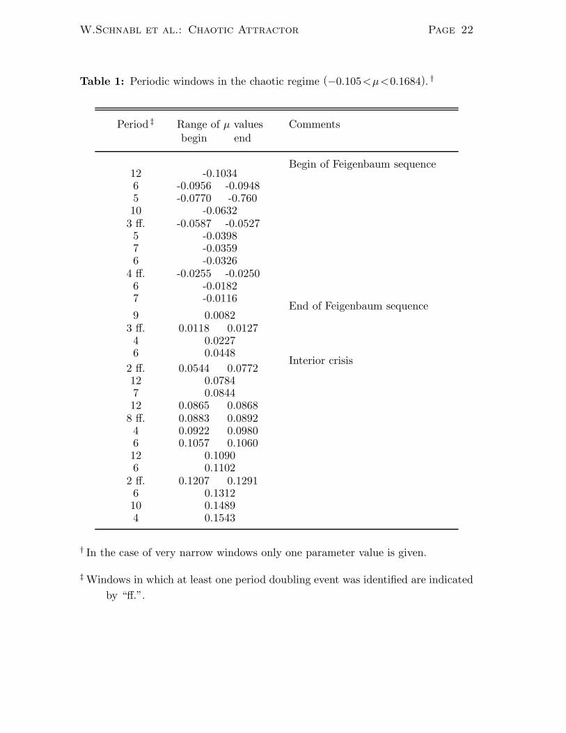
Table 1: Periodic windows in the chaotic regime (−0.105<µ<0.1684). †
Period ‡ Range of µ values Commentsbegin end
Begin of Feigenbaum sequence12 -0.10346 -0.0956 -0.09485 -0.0770 -0.76010 -0.0632
3 ff. -0.0587 -0.05275 -0.03987 -0.03596 -0.0326
4 ff. -0.0255 -0.02506 -0.01827 -0.0116
End of Feigenbaum sequence9 0.0082
3 ff. 0.0118 0.01274 0.02276 0.0448
Interior crisis2 ff. 0.0544 0.077212 0.07847 0.084412 0.0865 0.0868
8 ff. 0.0883 0.08924 0.0922 0.09806 0.1057 0.106012 0.10906 0.1102
2 ff. 0.1207 0.12916 0.131210 0.14894 0.1543
† In the case of very narrow windows only one parameter value is given.
‡ Windows in which at least one period doubling event was identified are indicated
by “ff.”.
W.Schnabl et al.: Chaotic Attractor Page 23
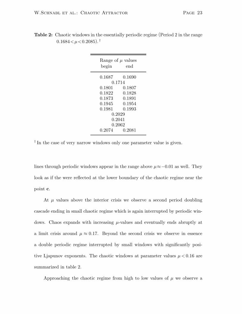
Table 2: Chaotic windows in the essentially periodic regime (Period 2 in the range
0.1684<µ<0.2085). †
Range of µ valuesbegin end
0.1687 0.16900.1714
0.1801 0.18070.1822 0.18280.1873 0.18910.1945 0.19540.1981 0.1993
0.20290.20410.2062
0.2074 0.2081
† In the case of very narrow windows only one parameter value is given.
lines through periodic windows appear in the range above µ≈−0.01 as well. They
look as if the were reflected at the lower boundary of the chaotic regime near the
point c.
At µ values above the interior crisis we observe a second period doubling
cascade ending in small chaotic regime which is again interrupted by periodic win-
dows. Chaos expands with increasing µ-values and eventually ends abruptly at
a limit crisis around µ ≈ 0.17. Beyond the second crisis we observe in essence
a double periodic regime interrupted by small windows with significantly posi-
tive Ljapunov exponents. The chaotic windows at parameter values µ < 0.16 are
summarized in table 2.
Approaching the chaotic regime from high to low values of µ we observe a
W.Schnabl et al.: Chaotic Attractor Page 24
periodic attractor appearing first at µ ≈ 0.21. This attractor changes – at some
points discontinuously – and small chaotic windows occur in the periodic regime
which remind of intermittence. Eventually chaos is reached in one step at µ≈0.17.
Fig. 10: Return maps one the unit interval corresponding to the Poincare
cross-section for different parameter values (ν =0).
A: µ=−0.101, B: µ=−0.029, C: µ=−0.002, D: µ=0.016,
E: µ=0.088 and F: µ=0.142.
For few selected values of the parameter µ we constructed return maps on the
unit interval which are shown in fig.10. As expected the maps resemble closely the
logistic map in the parameter range were we observe the Feigenbaum sequence. At
higher values of µ the map becomes more sophisticated and a second maximum
appears.
6.Mutation caused changes in the chaotic regime
Mutation is an unavoidable by-product of replication. Quantitative answers
to the questions if and how complex dynamics is changing under the influence
of mutation is of obvious importance for biological applications. Therefore we
performed a study of the influence of mutation on the chaotic attractor in the
replicator equation. Equ.(2) with rate constants Aij according to (9) was studied
by a version of perturbation theory [38] under the simplifying assumption of equal
mutation rates (Qij = ε for i 6= j; equ.(3) shows the definition of ε). The kinetic
W.Schnabl et al.: Chaotic Attractor Page 25
equations for replication and mutation are rewritten in such a way that error-free
production and mutant formation appear as additive contributions:
x = R(x) + M(x, ε) (27)
with Rk = xk
(
∑
j
Akjxj −∑
i,j
Aijxixj
)
and
Mk =∑
i,j
(
Qki(ε)Aijxixj − Qik(ε)Akjxkxj
)
.
The first part – the unperturbed equation – is identical with equ.(4). Mutation M
is considered as perturbation with ε being the pertubation parameter. The replica-
tor part is insensitive to the addition of constants to the reaction rate parameters:
Aij → Aij + ∆ [39] . In order to make the perturbation approach applicable to
equ.(9) we had to apply a sufficiently large value of this additive constant which
was chosen to be ∆=8.
The influence of mutation on the position of the kth fixed point of the unper-
turbed replicator equation (4) (x(0)k
) is expressed by
xk(ε) = x(0)k + ε · dk + O(ε2) . (28)
As shown in [38] the shift dk is obtained from
J(x(0)k ) · dk = −M(x
(0)k ) , (29)
where J(x) represents the Jacobian of the unperturbed system: Jij = ∂Ri
∂xj. In
table 3 we summarize the shifts of all important fixed points of our model replicator
equation determined by (9).
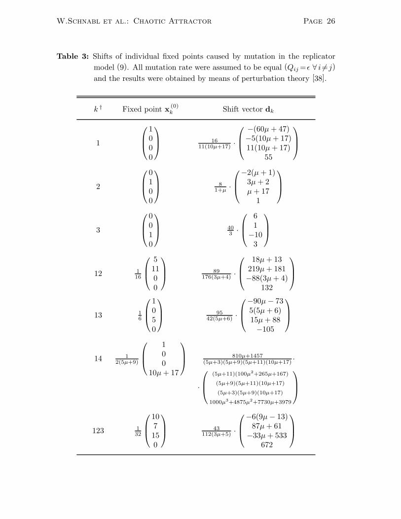
W.Schnabl et al.: Chaotic Attractor Page 26
Table 3: Shifts of individual fixed points caused by mutation in the replicator
model (9). All mutation rate were assumed to be equal (Qij =ε ∀ i 6=j)
and the results were obtained by means of perturbation theory [38].
k † Fixed point x(0)k Shift vector dk
1
1000
1611(10µ+17)
·
−(60µ + 47)−5(10µ + 17)11(10µ + 17)
55
2
0100
81+µ
·
−2(µ + 1)3µ + 2µ + 17
1
3
0010
403 ·
61
−103
12 116
51100
89176(3µ+4) ·
18µ + 13219µ + 181−88(3µ + 4)
132
13 16
1050
9542(5µ+6) ·
−90µ − 735(5µ + 6)15µ + 88−105
14 12(5µ+9)
100
10µ + 17
810µ+1457(5µ+3)(5µ+9)(5µ+11)(10µ+17)
·
·
(5µ+11)(100µ2+265µ+167)
(5µ+9)(5µ+11)(10µ+17)
(5µ+3)(5µ+9)(10µ+17)
1000µ3+4875µ2+7730µ+3979
123 132
107150
43112(3µ+5) ·
−6(9µ − 13)87µ + 61
−33µ + 533672
W.Schnabl et al.: Chaotic Attractor Page 27
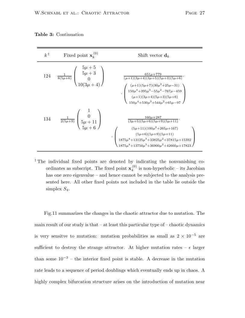
Table 3: Continuation
k † Fixed point x(0)k Shift vector dk
124 18(5µ+6)
5µ + 55µ + 3
010(3µ + 4)
651µ+779(µ+1)(3µ+4)(3µ+5)(5µ+3)(5µ+6)
·
·
(µ+1)(5µ+7)(30µ2+25µ−31)
150µ4+395µ3−55µ2−767µ−459
(µ+1)(3µ+4)(5µ+3)(5µ+6)
150µ4+530µ3+544µ2+65µ−97
134 12(5µ+9)
10
5µ + 115µ + 6
160µ+287(3µ+5)(5µ+6)(5µ+9)(5µ+11)
·
·
(5µ+11)(100µ2+265µ+167)
(5µ+6)(5µ+9)(5µ+11)
1875µ4+13125µ3+33825µ2+37815µ+15392
1875µ4+13750µ3+36900µ2+42660µ+17823
† The individual fixed points are denoted by indicating the nonvanishing co-
ordinates as subscript. The fixed point x(0)4 is non-hyperbolic – its Jacobian
has one zero eigenvalue – and hence cannot be subjected to the analysis pre-
sented here. All other fixed points not included in the table lie outside the
simplex S4.
Fig.11 summarizes the changes in the chaotic attractor due to mutation. The
main result of our study is that – at least this particular type of – chaotic dynamics
is very sensitve to mutation: mutation probabilities as small as 2 × 10⁻⁵ are
sufficient to destroy the strange attractor. At higher mutation rates – ε larger
than some 10−3 – the interior fixed point is stable. A decrease in the mutation
rate leads to a sequence of period doublings which eventually ends up in chaos. A
highly complex bifurcation structure arises on the introduction of mutation near
W.Schnabl et al.: Chaotic Attractor Page 28
the limit crisis of the unperturbed attractor. Fig.12 shows an enlarged portion
of fig.11 with a resolution of approximately 0.005 in µ and 5 × 10⁻⁷ in ε. At
the present stage of resolution we cannot say whether the bifurcation set forms a
fractal or not.
Fig. 11: Extension of the chaotic regime into the range of small mutation
rates.
Fig. 12: An enlargement of the bifurcation diagram near the limit crises
of the unperturbed replicator equation.
It is not surprising that even small mutation rates destroy the chaotic attractor
since the mutation term causes the saddle focus to move into the unphysical range
outside of the simplex S4 [38]. Therefore the trajectories can no longer come
sufficiently close to the saddle and Silnikov’s mechanism breaks down. Furthermore
the fixed point P12 moves into the interior of S4 and thus the limit crisis occurs
earlier.
7.Conclusions
The strange attractor in Lotka-Volterra and replicator systems of low di-
mension was fully characterized in a two-dimensional subspace of the twelve-
dimensional parameter space. We were able to show that both chaotic attractors
reported for these dynamical systems so far, lie within the same chaotic regime.
W.Schnabl et al.: Chaotic Attractor Page 29
There is no doubt that this regime extends also into other directions in parameter
space. Because of technical limitations we have to leave the systematic multi-
dimensional search as a project for the future. Still unanswered is also the question
whether or not other chaotic regimes exist in areas which are not connected to the
investigated one.
One cross-section through the chaotic regime was studied in great detail.
Along this path chaos developes in an almost perfect Feigenbaum scenario and
then it breaks down in several interior crises – a major one and a few minor
events – and ends in the final limit crisis. On further continuation along the path
one encounters a periodic regime with is intermitted by a few, very small chaotic
windows. The chaos is never fully developed: a small hole around the central –
unstable – fixed point remains always left out by the long-time trajectories. Right
in the centre of the chaotic regime the fractal set produced by the attractor is of
multi-fractal type. The distribution of dimensions covers a range from 1.3 to 3.
The replicator equation allows straight inclusion of mutation which inevitably
occurs in nature. The most relevant result we obtained in the present study is a
substantial reduction in the dynamical complexity with increasing mutation rates.
Strange attractors are replaced by stable closed orbits, limit cycles are converted
into stable attractors. It is interesting to note that we found a Feigenbaum se-
quence in opposite direction: reduction of the error-rate yields a cascade of bifur-
cations which eventually ends in the chaotic attractor of the unperturbed system.
We cannot claim – nor do we intend to – that increased mutation will always leads
W.Schnabl et al.: Chaotic Attractor Page 30
to simpler dynamics but general intuition favours this view: mutation can be un-
derstood as a force pushing trajectories towards the centre of the concentration
simplex. Wide excursions of trajectories which are characteristic for sophisticated
closed orbits and strange attractors are less likely if the attractor lives near the
centre.
Acknowledgements
Financial support was provided by the Austrian Fonds zur Forderung der
wissenschaftlichen Forschung (Project No.6864) and by the Stiftung Volkswagen-
werk (B.R.D.). Stimulating discussions with Prof.Dr.Harald Posch are gratefully
acknowledged. This work required extensive use of computers and we are par-
ticularly grateful for generous supply with CPU time at the IBM 3090-400 VF
mainframe computer of the EDV-Zentrum der Universitat Wien within the EASI
project of IBM and at the NAS 9160 mainframe computer of the IEZ Wien.
W.Schnabl et al. : References Page 31
References
[1] P.E.Kloeden and A.I.Mees, Bull.Math.Biol.47(1985) 697.
[2] A.Chhabra and R.V.Jensen, Phys.Rev.Lett.62(1989) 1327.
[3] A.M.Fraser, Physica 34D(1989) 391.
[4] E.Gutierrez and H.Almirall, Bull.Math.Biol.51(1989) 785.
[5] H.G.Schuster, Deterministic chaos – an introduction 2nd Ed.,
VCh-Verlagsges., Weinheim (B.R.D.) 1988.
[6] R.W.Leven, B.-P.Koch and B.Pompe, Chaos in dissipativen Systemen
F.Vieweg & Sohn, Braunschweig (B.R.D.) 1989.
[7] M.Eigen, Naturwissenschaften 58(1971) 465.
[8] M.Eigen and P.Schuster, The hypercycle – a principle of natural self-
organization. Springer-Verlag, Berlin 1979.
[9] P.Schuster and K.Sigmund, J.Theor.Biol.100(1983) 533.
[10] P.Schuster, Physica 22D(1986) 100.
[11] J.Hofbauer and K.Sigmund, The theory of evolution and dynamical systems
– mathematical aspects of selection. Cambridge University Press, Cam-
bridge (U.K.) 1988.
[12] P.Schuster, Physica Scripta 35(1987) 402.
[13] J.Hofbauer, Nonlinear Analysis. Theory, Methods & Applications 5(1981)
1003.
[14] S.Smale, J.Math.Biol.3(1976) 5.
[15] A.Arneodo, P.Coullet and C.Tresser, Physics Letters 79A(1980) 259.
[16] A.Arneodo, P.Coullet, J.Peyraud and C.Tresser, J.Math.Biol.14(1982) 153.
[17] R.R.Vance, Amer.Natur.112(1978) 797.
[18] M.E.Gilpin, Amer.Natur.113(1979) 306.
[19] J.F.C.Kingman, Mathematics of genetic diversity. CBMS NSF Regional
Conf.Ser.in Appl.Math.Vol.34. SIAM Philadelphia (Penn.) 1980.
[20] J.F.C.Kingman, J.Appl.Prob.15(1978) 1.
W.Schnabl et al. : References Page 32
[21] P.Schuster, K.Sigmund and R.Wolff, J.Math.Analysis and Applications
78(1980) 88.
[22] P.Schuster, P.Stadler, W.Schnabl and C.Forst, Dynamics of nonlinear auto-
catalytic reaction networks. Akademie-Verlag, Berlin 1990
[23] J.Guckenheimer and P.Holmes, Nonlinear oscillations, dynamical systems
and bifurcations of vector fields. Springer-Verlag, New York 1983,
pp.318-325.
[24] N.Samardzija and L.D.Greller, Bull.Math.Biol.50(1988) 465.
[25] C.Grebogi, E.Ott and J.A.Yorke, Physica 7D(1983) 181.
[26] I.M.Bomze, Biol.Cybern.48(1983) 201.
[27] P.F.Stadler and P.Schuster, Bull.Math.Biol.5*(1990) ***.
[28] S.Kim, S.Ostlund and G.Yu, Physica 31D(1988) 117.
[29] J.D.Farmer, E.Ott and J.A.Yorke, Physica 7D(1983) 153.
[30] G.Bennetin, L.Galgani, A.Giorgilli and J.-M.Strelcyn, Meccanica
15(1980) 9.
[31] A.Wolf, J.B.Swift, H.L.Swinney and J.A.Vastano, Physica 16D(1985) 285.
[32] P.Schuster, K.Sigmund and R.Wolff, J.Differential Equations 32(1979) 357.
[33] J.Hofbauer, P.Schuster and K.Sigmund, J.Math.Biol.11(1981) 155.
[34] P.Grassberger, Phys.Lett.97A(1983) 227.
[35] H.G.E.Hentschel and I.Procaccia, Physica 8D(1983) 453.
[36] T.C.Halsey, M.H.Jensen, L.P.Kadanoff, I.Procaccia and B.I.Shraiman,
Phys.Rev.A 33(1986) 1141.
[37] M.J.Feigenbaum, J.Statist.Phys.46(1987) 919.
[38] P.F.Stadler and P.Schuster, submitted to J.Math.Biol. (1990).
[39] J.Hofbauer, P.Schuster, K.Sigmund and R.Wolff, SIAM J.Appl.Math.
38(1980) 282.


![Belyakov Homoclinic Bifurcations in a Tritrophic Food Chain …math.bd.psu.edu/faculty/jprevite/REU07/yu.pdf · dT Dl] , (2.lc) where T is time, R and K are prey intrinsic growth](https://img.dokumen.tips/doc/110x75/5f4b0977817bbb35cd4c7834/belyakov-homoclinic-bifurcations-in-a-tritrophic-food-chain-mathbdpsuedufacultyjprevitereu07yupdf.jpg)