Full Analytical Sensitivities in NURBS based

Isogeometric Shape Optimization

Xiaoping Qian ∗

Illinois Institute of TechnologyChicago, IL 60062

February 27, 2010

Abstract

Non-uniform rational B-spline (NURBS) has been widely used as aneffective shape parameterization technique for structural optimization dueto its compact and powerful shape representation capability and its pop-ularity among CAD systems. The advent of NURBS based isogeometricanalysis has made it even more advantageous to use NURBS in shapeoptimization since it can potentially avoid the inaccuracy and labor-tediousness in geometric model conversion from the design model to theanalysis model.

Although both positions and weights of NURBS control points affectthe shape, until very recently, usually only control point positions areused as design variables in shape optimization, thus restricting the designspace and limiting the shape representation flexibility.

This paper presents an approach for analytically computing the fullsensitivities of both the positions and weights of NURBS control points instructural shape optimization. Such analytical formulation allows accu-rate calculation of sensitivity and has been successfully used in gradient-based shape optimization.

The analytical sensitivity for both positions and weights of NURBScontrol points is especially beneficial for recovering optimal shapes that areconical e.g. ellipses and circles in 2D, cylinders, ellipsoids and spheres in3D that are otherwise not possible without the weights as design variables.

Keywords: Shape optimal design, NURBS, Isogeometric analysis

1 Introduction

This paper presents an approach for analytically computing the full sensitivitiesof both the positions and weights of NURBS (non-uniform rational B-spline)control points in structural shape optimization.

∗Email address: qian@iit.edu.

1

Even since the work of Braibant and Fleury [1], B-spline and its generalizedrepresentation, NURBS, have been widely used in shape parameterization instructural optimization. It has become the method of choice for parameterizingfreeform shape in structural optimization [2] for two important reasons: 1)With a few control points, NURBS can represent complex freeform shape. Thealternative representation, the use of finite element nodes as design variables,would often lead to wiggly, irregular shape. Figure 1 gives one such example.2) The output of NURBS-based shape optimization can be directly linked toa computer-aided design (CAD) system since NURBS is the standard shaperepresentation underlying all major CAD software.

(a) Initial design (b) Optimized design

Figure 1: Optimized shape of a hole in a plate where elements nodes are usedas design variables. Figures are taken from [1].

The recent advent of NURBS based isogeometric analysis [3] has made iteven more advantageous to use NURBS in shape parameterization for designoptimization since NURBS can not only be used to represent the geometry, itcan also be used as a basis for approximating the physical fields. The use of theNURBS basis in finite element analysis has exhibited superior numerical prop-erties, e.g. in terms of per-degree-of-freedom accuracy, over traditional finiteelement analysis [3]. Further, the tri-variate B-spline representation has beenextended to represent both geometry and material composition in functionallygradient materials (FGM) parts [4] and used in the B-spline basis based gradedfinite element analysis of FGM objects [5]. It thus allows closer integration withCAD since the exact geometry and even material composition can be used inboth design and analysis through the NURBS representation.

NURBS represented shape is affected by both the positions and weights ofits control points. Figure 2 presents a 4 × 3 control net for a NURBS surfaceconsisting of 2 × 2 knot spans with degree 2 in ξ1 direction and degree 1 inξ2 direction. Figure 2.b shows when a control point changes its position fromQa to Qb, the underlying surface and knot spans change. Figure 2.c shows thesurface change and the knot span change when the weight of control point Q

2

changes from 1 to 0.5.

(a) Initial NURBS surface

Qa

Qb

(b) Modified NURBS surface

Q

wa = 1

wb = 0.5

(c) Modified NURBS surface

Figure 2: Both position and weight of a control point can change the NURBSsurface. a) The initial NURBS surface; b) Modified NURBS surface after theposition of control point Q is changed from Qa to Qb, c) Modified NURBSsurface after the weight of the control point Q is changed from wa = 1 andwb = 0.5.

Although both positions and weights of control points affect the NURBSgeometry, as demonstrated in Fig. 2, until very recently, usually only posi-tions of control points are used as design variables [1, 6, 7, 8, 9, 10]. In thesework, analytical sensitivities when used are only given for positions of controlpoints, thus they are referred to as partial sensitivity in this paper. Isogeometricanalysis has recently been successfully applied in structural shape optimization[11, 12] where, again, only analytical sensitivities for positions of control pointsare given.

Thus far, the use of both weights and positions of control points as designvariables has only occasionally been explored, e.g. in [13]. In particular, therehas been a lack of analytical formula for sensitivity calculation for shape opti-mization with both positions and weights of control points as design variables.A notable exception is very recent work in [14] where both control points andweights are used to optimize one-dimensional beam structures with sensitivitiesanalytically evaluated.

Analytical formula for computing the sensitivity of physical quantities overboth positions and weights is important for the following reasons:

3

• Analytical formulas leads to more accurate and efficient calculation ofderivative information required in gradient-based optimization. The finitedifference based method for gradient calculation suffers from the “step-size dilemma” due to the potential truncation error and round-off error[15]. It is also inefficient. If we need to find the derivatives of the struc-tural response with respect to n design variables, the forward-differenceapproximation requires n analyses, while the central-difference approxi-mation would require 2n analyses.

• The use of NURBS weights as design variables in structural optimization,in addition to positions of control points, lends more flexibility in shaperepresentation and enlarges the design space, which can lead to better de-sign. In particular, it makes it possible to recover a class of optimal shapessuch as conic curves, e.g. ellipses and circles, and surfaces, e.g. cylinders,spheres and ellipsoids, which are otherwise not possible. Note, withoutweights, NURBS shape degenerates into B-spline shape and B-spline rep-resentation cannot exactly represent these conic curves and surfaces.

The absence of analytical sensitivities of physical quantities such as compli-ance, displacement and stress over shape parameters, i.e. both positions andweights, is due perhaps to the seeming complexity of such a derivation. A naıveway of obtaining these sensitivities would be to expand the integrand involvedin calculating these physical quantities into explicit expressions of design vari-ables, which would be of daunting complexity. In the context of isogeometricshape optimization, the derivation could be more involving since the NURBSbasis function used in analysis also becomes affected by the design variables(weights). For example, although the usefulness of weights as design variableswas recognized in recent work in [11], the derivation of analytical sensitivitiesfor weights was not available and was deemed “more complex”.

In this paper, we give a set of compact formulas for computing analyticalsensitivities for both control point positions and weights, thus referred to as fullsensitivity. Our approach follows that of [16, 17, 18], an isoparametric basedtechnique for differentiating stiffness matrix and force vectors with respect todiscrete design variables. We use the chain rule of differentiation and Jacobi’sformula for the derivative of a determination to derive these compact formulas.These formulas are applicable to both traditional finite element based NURBSshape optimization and isogeometric shape optimization.

The calculation of these sensitivities involve two terms: analysis terms thatare encountered during the usual finite element analysis and isogeometric analy-sis and geometric sensitivities that are represented as the derivatives of positionsand weights over design variables. Mesh refinement is often required for accu-rate finite element analysis. This is especially true in isogeometric shape opti-mization since the weights are now design variables which can induce distorteddistribution of isoparametric curves (element boundaries). Thus, an analyticalmethod is also given for propagating geometric sensitivities of the control pointsin the design model to those of the control points in the refined analysis model.

4

Our numerical implementation is based on the isogeometric analysis due toits numerical advantages. Numerical examples demonstrate the availability ofsuch analytical formulas has both theoretical implication and practical signifi-cance. Theoretically, they can be used in interpreting the optimality conditionsand understanding behaviors of physical systems which may not been seen di-rectly from the problem. For example, they can be used in determining whetheran exact circle is the optimal shape for a hole in a plate under bi-axial load. Inpractice, they enlarge the design space, allow flexibility in shape representationand lead to better designs.

In the remainder of this paper, Section 2 gives a brief introduction on theNURBS basis and NURBS geometry and introduces some key notations usedin sensitivity derivation. Section 3 gives a general formulation of shape opti-mization and the role of sensitivity in shape optimization. Section 4 gives theanalytical formulas for sensitivities over positions and weights of NURBS con-trol points. Section 5 discusses how the geometric sensitivity of a design modelcan be analytically propagated to that in the refined analysis model. Section6 discusses the result of our numerical implementation on some common shapeoptimization problems. This paper concludes in Section 7. The derivation ofthe analytical formulas is given in the Appendix.

2 Introduction to NURBS

This section gives a brief introduction on NURBS basis functions and NURBSgeometry. It introduces some notations that will be used in deriving the ana-lytical sensitivity in following sections. For details on NURBS, refer to [19].

A NURBS curve of degree p is defined as follows

x(ξ) =∑ni=0Bi,p(ξ)wiPi∑nj=0Bj,p(ξ)wj

, 0 ≤ ξ ≤ 1, (1)

where Pi = (xi1 , xi2) represents the coordinate positions of a set of i = 0, . . . , ncontrol points, wi is the corresponding weight, and Bi,p is the degree p B-spline basis function defined on the knot vector

Ξ = ξ0, ξ1, . . . , ξn+p+1.

The i-th (i = 0, . . . , n) B-spline basis function can be defined recursively as

Bi,p(ξ) =(ξ − ξi)Bi,p−1(ξ)

ξi+p − ξi+

(ξi+p+1 − ξ)Bi+1,p−1(ξ)ξi+p+1 − ξi+1

Bi,0(ξ) =

1 ξi ≤ ξ ≤ ξi+1

0 Otherwise

.

The derivative of the i-th B-spline basis function can be computed as follows

dBi,p(ξ)dξ

=p

ξi+p − ξiBi,p−1(ξ)− p

ξi+p+1 − ξi+1Bi+1,p−1(ξ).

5

A NURBS surface of degree p in ξ1 direction and degree q in ξ2 direction isa bivariate vector-valued piecewise rational function of the form

x(ξ1, ξ2) =∑nk=0

∑ml=0Bk,p(ξ1)Bl,q(ξ2)wk,lPk,l∑n

s=0

∑mt=0Bs,p(ξ1)Bt,q(ξ2)ws,t

, 0 ≤ ξ1, ξ2 ≤ 1 (2)

The Pk,l form a (n + 1) × (m + 1) bidirectional control net, wk,l are theweights, and the Bk,p and Bl,q are the B-spline basis functions defined onthe knot vectors Ξ1 and Ξ2.

Without loss of generality, we here consider a NURBS surface on a knot-span basis, defined by an array of nen = (p+ 1)× (q + 1) control points. Note,the NURBS basis function has local influence property, i.e. within a given knotspan, only (p + 1) × (q + 1) number of non-zero basis functions. So the totalnumber of nodes per element (knot span) is nen = (p+ 1)× (q + 1).

The NURBS basis function Nk,l for the control point Pk,l (k = 0, . . . , n andl = 0, . . . ,m) can be written as

Nk,l(ξ1, ξ2) =Bk,p(ξ1)Bl,q(ξ2)wk,l∑n

s=0

∑mt=0Bs,p(ξ1)Bt,q(ξ2)ws,t

(3)

where p and q are degrees of the non-rational B-spline basis functions Bk,p andBl,q.

For notational convenience, we change the matrix form of the NURBS basisfunction into the column form by converting the matrix index (k, l) into a columnindex i = k ∗ (q+1)+ l. We further note the NURBS basis in the following form

Ri(ξ1, ξ2) = Bk,p(ξ1)Bl,q(ξ2),

Ni(ξ1, ξ2) =RiwiRTW

,

where R and W represents the column collection of Ri and wi for i = 1 to nen.We thus can rewrite Eq. (2) as

x(ξ1, ξ2) = NTP =nen∑i=1

NiPi. (4)

The derivative of Ri over its parametric coordinates can then be computedas

∂Ri∂ξ1

=dBk,p(ξ1)

dξ1Bl,q(ξ2),

∂Ri∂ξ2

= Bk,p(ξ1)dBl,q(ξ2)dξ2

(5)

3 Shape optimization

We use a 2D elasticity problem as an example for shape optimization and giveits weak form equilibirum equations. The terms in the weak form such asstiffness matrix and force vectors will be used in composing objective functionsand constraints for structural shape optimization.

6

3.1 Linear elasticity analysis

We here consider a 2D linear elasticity problem. The strong form for linearelasticity [20] is as follows

∇ · σx + bx = 0 and ∇ · σy + by = 0 on Ωσ = D∇suσx · n = tx and σy · n = ty on Γt,u = u on Γu.

where Γt is portion of the boundary where traction is specified and Γu is portionof the boundary where displacement is specified.

The underlying discrete equilibrium equation is

Ku = f .

where K is the stiffness matrix, u is the displacement vector and f is the externalforce vector. The stiffness matrix K can be assembled from the element stiffnessmatrix Ke. Likewise, the force vector f can be assembled from the element forcevector fe.

The element stiffness matrix is computed as follows.

Ke = te

∫Ωe

BTDB|J|dΩ (6)

where te is the plate element thickness and Ω is the parametric domain of thestructure in the ξ1ξ2 space.

The integral is integrated numerically by determining the value of the inte-grand at Gauss points in the element. The strain-displacement matrix B is

B =

∂N1

∂x10 ...

∂Nnen

∂x10

0∂N1

∂x2... 0

∂Nnen

∂x2

∂N1

∂x2

∂N1

∂x1...

∂Nnen

∂x2

∂Nnen

∂x1

(7)

where Ni is the basis function for finite element analysis and is the NURBSbasis function in isogeometric analysis.

For plane stress, the stress strain matrix D is written as

D =E

1− v2

1 v 0v 1 00 0 1−v

2

.where E is Young’s modulus and v is Poisson’s ratio.

7

The Jacobian matrix is given by

J =

∂x1

∂ξ1

∂x2

∂ξ1∂x1

∂ξ2

∂x2

∂ξ2

(8)

which maps the points from the parametric coordinates to the world coordinates.The force vector on element e may be written

fe =∫

Ωe

NTb|J|tedΩ +∫

Γte

NT t|J|dΓ (9)

where b is the body force (force per unit area), t is the traction on the boundary,and Γt is the parametric domain of the traction boundary in the ξ1ξ2 space.

3.2 Structural shape optimization

The general mathematical formulation of a structural optimization problem canbe stated as follows

minαs

f(u(α),α)

s.t. hi(u(α),α) = 0, i = 1 to nhgj(u(α),α) ≤ 0, j = 1 to ngαmins

≤ αs ≤ αmaxs, s = 1 to neq

,

where the objective function f is a function of the state variable, e.g. displace-ment u and the design variables α, nh is the number of equality constraints,ng is the number of inequality constraints, and neq is the number of designvariables. The behavior constraints are represented by equality and inequalityconstraints hi and gj .

To solve the generally nonlinear optimization problem, both gradient basedand gradient-less methods can be applied. In this paper, we focus on a gradientbased approach where both the structural response and its sensitivity over designchange is required. The specific optimization algorithm used in this paper isthe gradient-based method of moving asymptotes (MMA) [21].

For example, a commonly used design formulation for structural shape op-timization is to minimize the mean compliance of a structure under a fixedamount material through a volume fraction constraint V ≤ V ∗. Its discreteform reads

minα

f = fTu

s.t. V ≤ V ∗Ku = f

.

Another objective function used in this paper is to minimize the displacementat the point of load under a volume fraction constraint, i.e.

minα

f = lTu

s.t. V ≤ V ∗Ku = f

8

where l is a zero vector with a 1 corresponding to the point of load.Using the gradient-based optimization approach such as MMA to solve the

above optimization problems requires the sensitivities of objective functionsand constraints over the design variables, i.e. ∂f/∂α, ∂hi/∂α and ∂gj/∂α.Evaluating these sensitivities requires sensitivities of physical quantities such asthe stiffness K and force vector f over the design variables.

4 Sensitivity analysis

Sensitivity is useful in evaluating the robustness of a particular design and indetermining search directions during structural optimization. During the op-timization process, the geometric domain Ωe will change due to the change ofdesign variables α, however the corresponding parametric domain Ωe does notunder certain constraints such that the mesh remains in a good quality. Thiscan be ensured by checking the Jacobian of the mapping.

Since the plate thickness te and the stress-strain matrix D are constant,differentiation of Eq. (6) gives

∂Ke

∂αs=∫

Ωe

(∂BT

∂αsDB|J|+ BTD

∂B∂αs|J|+ BTDB

∂|J|∂αs

)te dΩ. (10)

Differentiating Eq. (9) gives

∂fe∂αs

=∫

Ωe

(∂NT

∂αsb|J|+ NT

(∂b∂x1

∂x1

∂αs+

∂b∂x2

∂x2

∂αs

)|J|+ NTb

∂|J|∂αs

)tedΩ

+∫

Γte

(∂NT

∂αst|J|+ NT

(∂t∂x1

∂x1

∂αs+

∂t∂x2

∂x2

∂αs

)|J|+ NT t

∂|J|∂αs

)dΓt

.

(11)Our goal is now to find analytical formulas for ∂BT /∂αs, ∂|J|/∂αs, ∂N/∂αs

and ∂x/∂αs.

4.1 Full Analytical Sensitivity in NURBS IsogeometricShape Optimization

First, we define two additional matrices:

G =

∂N1∂x1

∂N2∂x1

...∂Nnen

∂x1

∂N1∂x2

∂N2∂x2

...∂Nnen

∂x2

,G =

∂N1∂ξ1

∂N2∂ξ1

...∂Nnen

∂ξ1

∂N1∂ξ2

∂N2∂ξ2

...∂Nnen

∂ξ2

.In the following, for notational convenience, let us denote ∂/∂αs by a prime

(′) and the derivative over ξj , ∂()/∂ξj , as as (),ξj. Note, if we know G′, B′ can

be drawn from it.

9

Thus for the calculation of the sensitivities of stiffness matrix and forcevector over design variables αs, it suffices to find expressions for N′, G′, x′, and|J|′.

We present below our results concerning analytical sensitivities for shapeoptimization based on NURBS isogeometric analysis. The detailed proof isprovided in the Appendix.

Theorem 1 (Full sensitivity for P and W in isogeometric optimization)

|J|′ = |J|tr(GP′ + J−1G′P

), (12)

G′ = J−1G′(I−PG)−GP′G, (13)

x′ = NTP′ + (N′)TP, (14)

N ′i =Riw

′i

RTW− RiwiRTW′

(RTW)2, (15)

(Ni,ξj

)′ =Ri,ξjw

′i

RTW−Ri,ξjwiR

TW′ +Riw′i(R,ξj )TW +Riwi(R,ξj )TW′

(RTW)2

+ 2Riwi(R,ξj )TWRTW′

(RTW)3. (16)

Note, I is an identity matrix.(Ni,ξj

)′ in Eq. (16) is used in describing G′. In-serting the above equations into Eqs. (10) and (11) gives the complete analyticalsensitivities of stiffness matrix and force vector over the design variables. Sinceboth the effect of positions P and weights W of control points are considered,we thus refer to the resulting sensitivity as total sensitivity.

Such sensitivity information reflects the effect of change from both controlpoint positions and weights. It should be pointed out, although we present theseformulas in the context of a 2D elasticity problem, they are exactly applicableto 3D problems. To the author’s best knowledge, this is the first reportedanalytical sensitivity for NURBS based shape optimization, taking into accountthe effect of the NURBS weights and control points.

If the weights do not change with respect to design variables, i.e. w′i = 0,this leads to N ′i = 0 and

(Ni,ξj

)′ = 0, and thus G′ = 0. The above sensitivityequations would then become a partial sensitivity for P as follows.

Corollary 2 ( Partial sensitivity for P in isogeometric optimization)

|J|′ = |J|tr(GP′),|G|′ = −GP′G,

x′ = NTP′,

N′ = 0,(Ni,ξj

)′ = 0,

which are identical to the forms presented in [17, 18], except that instead ofusing nodal coordinates, we use control points’ coordinates P and instead of

10

using the Lagrange basis function in FEA, we use the NURBS basis functionin isogeometric analysis. In this sense, the full sensitivity presented in Theo-rem 1 generalizes the sensitivity in structural optimization from the classicalLagrange shape function based isoparametric finite element analysis where thebasis functions do not change with respect to design variables to NURBS basedisogeometric analysis where the basis functions could change.

The total analytical sensitivities presented in Theorem 1 can also be ex-tended to traditional finite element based shape optimization. In traditionalFEA, the Lagrange basis function does not change w.r.t to the design vari-ables, i.e. N ′i,ξj

= 0, we thus have the following corollary for total analyticalsensitivities for both P and W in FEA based shape optimization:

Corollary 3 ( Full sensitivity for P and W in FEA based optimization)

|J|′ = |J|tr(GP′),|G|′ = −GP′G,

x′ = NTP′,

N ′i =Riw

′i

RTW− RiwiRTW′

(RTW)2,(

Ni,ξj

)′ = 0,

In Corollary 3, the sensitivities for both positions and weights of control pointsare given. The term x′ and consequently the term N ′i are needed to calculatethe physical coordinates’ derivatives over the design variables, e.g. in the bodyforce term in Eq. 11 and in structural grid generation where element nodes aregenerated from a NURBS representation.

The significance of Theorem 1 on total sensitivities for both P and W isobvious for the following reasons.

• Low computational overhead : the terms used in Eqs. (12) - (16) canbe divided into two parts: 1) Geometric sensitivity as represented byP′ and W′, which measures the sensitivities of positions and weights ofNURBS control points over design variables. These terms are thus referredto as geometric sensitivity in NURBS geometric optimization since theNURBS shape can be completely characterized by P and W for givendegrees and knot vectors in the NURBS geometry. 2) analysis terms. Allthe remaining terms are calculations already incurred during the usualisogeometric or finite element analysis. Together, geometric sensitivity inconjunction with the calculations incurred during the usual analysis leadsto physical sensitivity, thus low computational overhead is required in theanalytical sensitivity analysis. That is, to compute sensitivities of physicalquantities such as mass, stiffness and force, all the extra terms we needare the derivatives of control points P and weights W with respect todesign variables. The computational implementation of these analyticalsensitivities only takes a few extra lines of code.

11

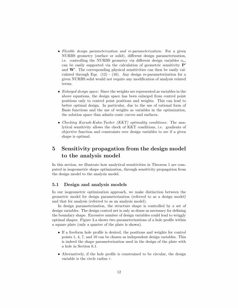
• Flexible design parameterization and re-parameterization: For a givenNURBS geometry (surface or solid), different design parameterization,i.e. controlling the NURBS geometry via different design variables αs,can be easily supported via the calculation of geometric sensitivity P′

and W′. The corresponding physical sensitivities can then be easily cal-culated through Eqs. (12) - (16). Any design re-parameterization for agiven NURBS solid would not require any modification of analysis relatedterms.

• Enlarged design space: Since the weights are represented as variables in theabove equations, the design space has been enlarged from control pointpositions only to control point positions and weights. This can lead tobetter optimal design. In particular, due to the use of rational form ofBasis functions and the use of weights as variables in the optimization,the solution space thus admits conic curves and surfaces.

• Checking Karush-Kuhn-Tucker (KKT) optimality conditions: The ana-lytical sensitivity allows the check of KKT conditions, i.e. gradients ofobjective function and constraints over design variables to see if a givenshape is optimal.

5 Sensitivity propagation from the design modelto the analysis model

In this section, we illustrate how analytical sensitivities in Theorem 1 are com-puted in isogeometric shape optimization, through sensitivity propagation fromthe design model to the analysis model.

5.1 Design and analysis models

In our isogeometric optimization approach, we make distinction between thegeometric model for design parameterization (referred to as a design model)and that for analysis (referred to as an analysis model).

In design parameterization, the structure shape is controlled by a set ofdesign variables. The design control net is only as dense as necessary for definingthe boundary shape. Excessive number of design variables could lead to wrigglyoptimal shapes. Figure 3.a shows two parameterizations of a hole profile withina square plate (only a quarter of the plate is shown).

• If a freeform hole profile is desired, the positions and weights for controlpoints 1, 4, 7, and 10 can be chosen as independent design variables. Thisis indeed the shape parameterization used in the design of the plate witha hole in Section 6.1.

• Alternatively, if the hole profile is constrained to be circular, the designvariable is the circle radius r.

12

In each case, the geometric sensitivities of 12 control points P and the corre-sponding weights W in Figure 3.a can be derived with respect to the respectivedesign variables. Once P′ and W′ are known, they can be used in conjunctionwith the the design model based analysis terms in equations (12) to (16) tocompute physical sensitivities such as K′ and f ′.

123

45

6,

7

8

9

10

11

12

r

l

(a) Design parameterization (b) Analysis refinement

Figure 3: Design parameterization of a hole profile in a plate and the refinedanalysis model. Only a quarter of the plate is shown. a) Design model usedin shape parameterization; b) Analysis model through the refinement from thedesign model. Bold blues lines mark the element boundaries and red circles arecontrol points.

However, the mesh at such density is likely not sufficient for accurate analysisrequired in optimization. This is especially true, given the fact that the weightsare now design variables which can distort the isoparametric curve (elementboundaries). Numerical results in Section 6 will further attest to this. Thus,the analysis model often requires much finer mesh. Mesh refinement techniquessuch as h-refinement, p-refinement, and k-refinement [3] can be used for thispurpose. Figure 3.b shows an analysis model that is resulted from the origi-nal design model through knot insertion in both ξ1 and ξ2. The design modelconsists of 2 × 1 elements. The analysis model now consists of 4 × 2 elementsand has 24 control points and corresponding weights. With such mesh refine-ment, sensitivity propagation is then needed that can automatically calculatethe geometric sensitivities of control point positions and weights in the analysismodel (i.e. the 24 control points in Fig. 3.b) based on the information on thegeometric sensitivities of control point positions and weights in the design model(i.e. the 12 control points in Fig. 3.a). The subsection below describe how suchsensitivity propagation can be conducted.

13

5.2 Sensitivity propagation from the design model to theanalysis model

Here we focus on the sensitivity propagation during h-refinement. Sensitivitypropagation formulation for other refinement can be derived similarly.

The basic procedure for h-refinement is through knot insertion. We describebelow first the knot insertion for a B-spline curve, then its extension to a NUBRScurve.

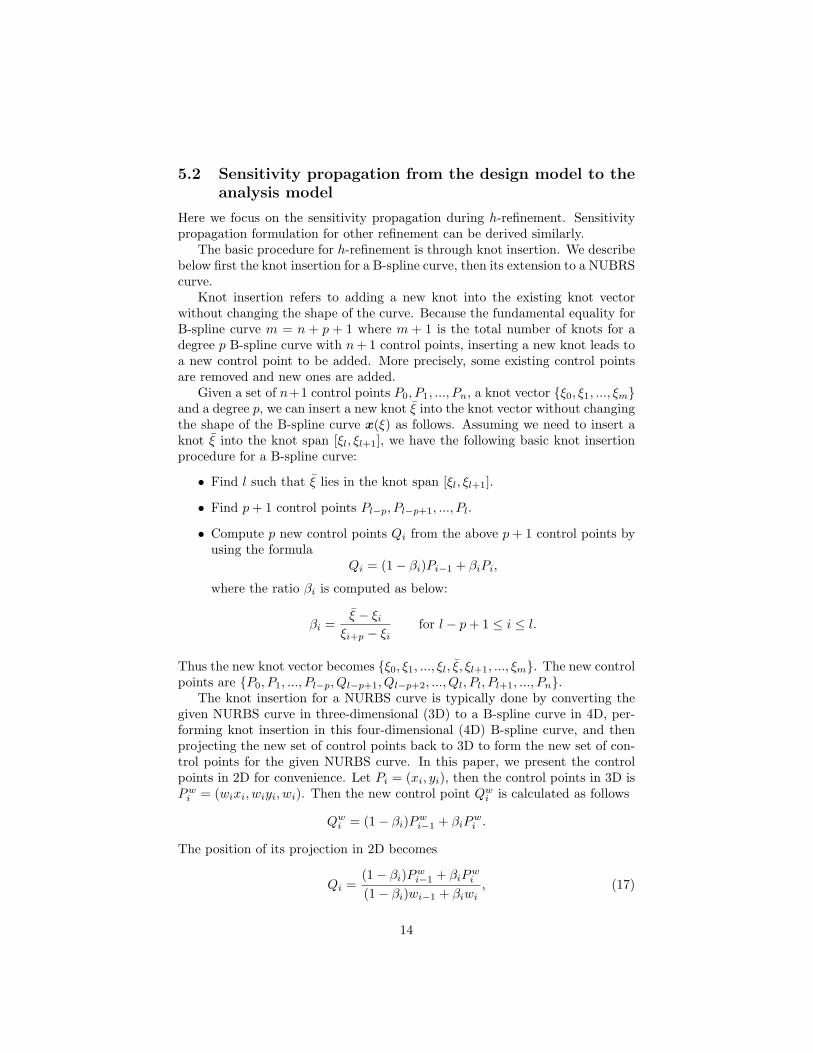
Knot insertion refers to adding a new knot into the existing knot vectorwithout changing the shape of the curve. Because the fundamental equality forB-spline curve m = n + p + 1 where m + 1 is the total number of knots for adegree p B-spline curve with n+ 1 control points, inserting a new knot leads toa new control point to be added. More precisely, some existing control pointsare removed and new ones are added.

Given a set of n+1 control points P0, P1, ..., Pn, a knot vector ξ0, ξ1, ..., ξmand a degree p, we can insert a new knot ξ into the knot vector without changingthe shape of the B-spline curve x(ξ) as follows. Assuming we need to insert aknot ξ into the knot span [ξl, ξl+1], we have the following basic knot insertionprocedure for a B-spline curve:

• Find l such that ξ lies in the knot span [ξl, ξl+1].

• Find p+ 1 control points Pl−p, Pl−p+1, ..., Pl.

• Compute p new control points Qi from the above p+ 1 control points byusing the formula

Qi = (1− βi)Pi−1 + βiPi,

where the ratio βi is computed as below:

βi =ξ − ξi

ξi+p − ξifor l − p+ 1 ≤ i ≤ l.

Thus the new knot vector becomes ξ0, ξ1, ..., ξl, ξ, ξl+1, ..., ξm. The new controlpoints are P0, P1, ..., Pl−p, Ql−p+1, Ql−p+2, ..., Ql, Pl, Pl+1, ..., Pn.

The knot insertion for a NURBS curve is typically done by converting thegiven NURBS curve in three-dimensional (3D) to a B-spline curve in 4D, per-forming knot insertion in this four-dimensional (4D) B-spline curve, and thenprojecting the new set of control points back to 3D to form the new set of con-trol points for the given NURBS curve. In this paper, we present the controlpoints in 2D for convenience. Let Pi = (xi, yi), then the control points in 3D isPwi = (wixi, wiyi, wi). Then the new control point Qwi is calculated as follows

Qwi = (1− βi)Pwi−1 + βiPwi .

The position of its projection in 2D becomes

Qi =(1− βi)Pwi−1 + βiP

wi

(1− βi)wi−1 + βiwi, (17)

14

and the weight iswQi = (1− βi)wi−1 + βiwi. (18)

Equations (17) and (18) form the basis for sensitivity propagation, i.e. prop-agating the sensitivity of control point position Pi and weight wi over designvariable αs, i.e. (P ′i , w

′i), to the new control point Qi and wQi

after the knotinsertion, i.e. (Q′i, w

′Qi

).From Eq. (18), we know

w′Qi= (1− βi)w′i−1 + βiw

′i. (19)

From Eq. (17) and the new sensitivity for the weight wQi, we have

Q′i =(1− βi)

(P ′i−1wi−1 + Pi−1w

′i−1

)+ βi (P ′iwi + Piw

′i)

wQi

− (1− βi)Pi−1wi−1 + βiPiwiw2Qi

w′Qi

. (20)

Therefore equations (18), (19), and (20) give all necessary equations forsensitivity propagation for h-refinement of a NURBS curve. A NURBS surfaceis defined with an array of control points and knot vectors. By repeating theabove knot insertion procedure and the sensitivity propagation to all rows andall columns of control points, sensitivity propagation can thus be applied to 2Dsurface, and similarly to a tri-variate NURBS volume in 3D.

6 Computational examples

In this section, we present three numerical examples that use our full analyticalsensitives for shape optimization. These examples, drawn primarily from [11],are commonly used examples in the shape optimization literature [22, 23, 24].

All problems are under plane stress conditions and the plate thickness te =1.0. Unless otherwise specified, the convergence criteria used is the change ofobjective function values, i.e.

ε =∣∣∣∣f (k) − f (k−1)

f (0)

∣∣∣∣where f (k) is the objective function value at the k−th iteration.

For the sake of simplicity in implementation, when mesh refinement is used,knots are recursively inserted at the parametric middle-point of every knot span.

6.1 Design of a plate with a hole

We begin our numerical examples with a classic shape optimization problem:optimizing the hole profile in a large plate under a biaxial stress field. Theobjective is to minimize the plate compliance under the constraint of material

15

volume. For an infinitely large plate, this problem has an analytical solution:circle under symmetric load and ellipse under asymmetric load. This makes itespecially suitable to examine the role of weights in shape optimization since,without varying weights, NURBS degenerates into non-rational B-spline andcannot represent conic sections exactly.

The initial design, including the structural dimensions and loads, is shownin Fig. 4. It is modeled as a bi-quadratic NURBS surface with 4 × 3 controlpoints. The knot vectors are 0,0,0,0.5,1,1,1 and 0,0,0,1,1,1, thus leading to2× 1 knot spans. The Young’s modulus is 210 and Poisson’s ratio is 0.3.

σy = 2.5

σx = 2.5

a = 75 b = 25

AB

CD

Figure 4: Initial design for a hole in a plate.

Design with both positions and weights

In this example, to ensure the optimality condition, we use the KKT normused in the MMA algorithm as the termination criteria and it should be lessthan 6.0e-6. We optimize the hole shape under two different volume fractionconstraints: V ≤ V ∗, 1) V ∗ = 96% and 2) V* = 99%. Here ’%’ refers to thepercentage of the total volume (10, 000) of the square plate without the hole.

For the first type of design with the volume constraint V ∗ = 96%, the initialhole shape is a straight line (Fig. 5). The model is refined 3× 4 times, leadingto (2 × 23) × (1 × 24) elements (knot spans). The optimization is conductedwith 8 design variables, including x-coordinates for control points A,B,C andy-coordinates for control points B,C,D and weights for control points B,C.The optimized design is shown in Fig. 5. In addition, following the work in [11],we also optimized the hole profile by pre-setting the control points for node Band C as wB = wC = 1 (with these weights, the NURBS curve degenerates intoa B-spline curve) and wB = wC = (1+

√2/2)/2 (with these weights, the NURBS

curve can exactly represent the circular profile). We plot the three optimized

16

(a) Initial design (b) Optimized design

(c) Local view of optimized design

Figure 5: Hole profile optimization under V ∗ = 96% with both control pointsand weights as design variables.

17

Table 1: Optimal designs under the constraint V ∗ = 96%

Type Iteration Compliance Volume

Theoretical N/A 466.5701 9600.0000Initial N/A 462.5555 9687.5000

8 variables, 23 466.5699 9599.99976 variables, wB = wC = 1 31 466.5708 9599.9996

6 variables, wB = wC = 0.8536 31 466.5701 9599.9996

profiles and the exact circule arc in Fig. 5.b. Visually speaking, the differencesamong the four profiles are indiscernable. In the view (Fig. 5.c) magnified ata scale comparable to that in [11], even though the control points are differentfor the three sets of optimized profiles, due to the influence of the weights, thehole profiles remain inseparable . This higher accuracy than that in [11] can beascribed to the use of refined analysis model in our optimization.

The detailed comparison of compliance for the initial design, the optimizeddesigns, and iteration times are shown in Table 1. This table demonstratesthat optimization with both positions and weights of control points as designvariables leads to smaller objective function value, i.e. compliance, than thosewithout.

(a) Initial design (b) Optimized design

Figure 6: Hole profile optimization under V ∗ = 99% with both control pointsand weights as design variables. Red circles are control points for the designmodel. The blue curves are knot curves of the refined analysis model.

For the second type of design with the volume constraint V ∗ = 99%, theinitial hole shape and the final optimized shape after mesh refinement are shownin Fig. 6. Note, the initial 2×1 knot spans undergo 4×5 subdivisions, leading to(2×24)×(1×25) elements. Again, this optimized design with 8 design variablesis compared with designs optimized with only control point positions as designvariables and weights are set at 1 and (1 +

√2/2)/2 for control point B,C. The

18

Table 2: Optimal designs under the constraint V ∗ = 99%

Type Iteration Compliance Volume

Theoretical N/A 428.7086 9900.0000Initial N/A 428.1381 9910.5851

8 variables 6 428.7087 9899.99976 variables wB = wC = 1 5 428.7092 9899.9995

6 variables wB = wC = 0.8536 5 428.7087 9899.9995

detailed comparison of the optimization results and iteration times for thesedesigns are shown in Table 2. Again, optimization with both positions andweights of control points as design variables leads to smaller objective functionvalue, i.e. compliance, than those without.

0 0.2 0.4 0.6 0.8 122.52

22.53

22.54

22.55

22.56

22.57

22.58

22.59

22.6

22.61

u = [0,1]

Rad

ial d

ista

nce

TheoreticalNURBSB-splineNURBS with specified weight

Figure 7: Radial distances from optimized holes to the circle center with bothcontrol points and weights as design variables. These holes are derived fromdifferent shape representations under V ∗ = 96%.

Since the four profiles (theoretical circular arc, the NURBS profile optimizedwith 8 design variables, the B-spline profile optimized with 6 design variablesand weights set to 1, and the NURBS profile optimized with 6 design variablesbut wB = wC = (1 +

√2/2)/2) are so close under each volume constraint, we

plot in Fig. 7 and Fig. 8 the radial distances from points on these four curvesto the theoretical circle center. Figure 7 shows, with V ∗ = 96%, the deviationfrom the theoretical circle is about 0.33% percent for the B-spline representation(6 design variables) derived design and 0.18% for the NUBRS representation (8design variables) derived design.

As V ∗ approaches 1, the finite plate approximates the infinite plate betterand we thus expect the optimal profile closer to an exact circle. Figure 8 shows,

19

0 0.2 0.4 0.6 0.8 111.255

11.26

11.265

11.27

11.275

11.28

11.285

11.29

11.295

11.3

u = [0,1]

Rad

ial d

ista

nce

TheoreticalNURBSB-splineNURBS with specifiedweight

Figure 8: Radial distances from optimized holes to the circle center with bothcontrol points and weights as design variables. These holes are derived fromdifferent shape representations under V ∗ = 99%.

with V ∗ = 99% , the deviation is approximately 0.33% for the B-spline represen-tation ( 6 design variables) derived design while less than 0.08% for the NUBRSrepresentation (8 design variables) derived design. That is, for NURBS rep-resentation derived optimal designs, the deviations have become smaller fromV ∗ = 96 to V ∗ = 99, yet this is not true for B-spline representation derivedoptimal designs. This is perhaps due to the fact B-spline cannot represent ac-curately the circular profile. For the NURBS representation with pre-specifiedweights (wB = wC = (1 +

√2/2)/2), the deviation on the resulting profile is

about the same as that on the NURBS repersentation derived profile. This fur-ther illustrates the significance of the use of weights as design variables in shapeoptimization.

Design with weights

Due to the use of both weights and positions of control points as design variables,the optimized profiles in the previous subsection are closer to the exact circlethan those with positions only as design variables. In order to better understandand examine if exact circles can be recovered, we use the weights of Point Band Point C as design variables, and positions of control points are set forrepresenting the exact circle and satisfying the volume constraint (Fig. 9). Thisfigure shows the initial design with volume constraint of 96% and all weightsare set to 1. The termination criteria is KKTnorm from the MMA code to besmaller than 1.0e-6. In the optimization, the initial model is subdivided 2 × 3times for analysis.

Figure 10 shows, at three different initial conditions, 1) wB = wC = 0.1, 2)wB = wC = 10, and 3) wB = 0.1, and wc = 10, the optimized profiles recover

20

B

C

Figure 9: Control point positions for optimization with wB and wC as designvariables.

well the exact circle (Fig. 9.d). Table 3 shows the recovered weights under theseinitial conditions. They deviate from the nominal weights (1 +

√(2)/2)/2 =

0.853553391 for an exact circle less than 0.0001. Since the optimized profiles inthe previous experiment have been shown to be very close to the exact circle, itis of no surprise that exact weights can be very well recovered.

Table 3: Recovered weights under different initial conditions

w(0)B w

(0)C Iteration (k) w

(k)B w

(k)C

0.1 0.1 5 8.535909e-001 8.535909e-00110 10 8 8.535914e-001 8.535914e-0010.1 10 12 8.535274e-001 8.536550e-001

Design with weights under asymmetric loads

We extend the above design with weights as design variables to design underasymmetric loads, i.e. σx = −5 and σy = 2.5. The theoretical prediction for aninfinite plate is that the optimal hole is an ellipse with the ratio of major/minoraxes equals to that of the load.

Figure 11 shows the initial position of the hole with weights wB = 0.1,wC = 10 and the resulting design under the volume constraint V ∗ = 96%.Similar optimizations have been done for different volume constraints. Theresults are described in Table 4 where w0

B = w0C = (1+

√2/2)/2. The KKT norm

1.0e-6 is used for convergence termination. The analysis meshes are obtainedwith 4 × 5 subdivisions from the initial NURBS model, except for the 99.9%volume constraint with 4× 6 subdivisions. The optimizations all converge after9 to 12 iterations.

21

(a) Initial weight: 0.1 and 0.1 (b) Initial weight: 10 and 10

(c) Initial weight: 0.1 and 10 (d) Optimized design

Figure 10: Design optimization with weights as design variables under differentinitial conditions. Red circles are control points for the design model. The bluecurves are knot curves in the refined analysis model.

22

(a) Initial design (b) Optimized design

Figure 11: Optimized design under asymmetric load with V ∗ = 96% withweights as design variables. The red profile is an exact ellipse satisfying thevolume constraint.

δ1

δ2

(a) general trend

(b) Magnified view of Fig. 11.b nearcontrol point B

(c) Magnified view of Fig. 11.b nearcontrol point C

Figure 12: Optimized hole shape under asymmetric load with weights as designvariables. Dotted red curve representing the exact ellipse.

23

Table 4: Optimal designs under asymmetric load

Volume fraction wB wC (wB − w0B)/w0

B (wC − w0C)/w0

C

85% 0.78752 0.99992 -7.74% 17.15%90% 0.78772 0.99880 -7.71% 17.02%96% 0.81705 0.90446 -4.28% 5.96%99% 0.84072 0.86822 -1.50% 1.72%

99.5% 0.84148 0.86756 -1.41% 1.64%99.9% 0.84373 0.86748 -1.15% 1.63%

Table 4 shows the computational results for the finite-dimensioned platenearly agree with the optimal result of the infinite plate. Note, the optimaldesigns for the finite and infinite plates are distinct [24, 25]. As the hole be-comes smaller (the volume fraction of the solid approaches unity), the differencebetween the two sets of optimal design also become smaller as seen in Table 4.At 99.9%, the errors for the weights of the point B and point C are about alittle over one percent.

An interesting trend can also be observed in Table 4: wB is consistentlybelow the weight for the exact ellipse and wC consistently above it. As thevolume fraction for the solid increases, the deviations become smaller. Thissuggests the optimal shape for a finite plate under asymmetric load would lookas exaggerated in Fig. 12.a. As the volume fraction increases, δ1 and δ2 repre-senting the deviation to the exact ellipse as shown in Fig. 12.a become smaller.A magnified view of the optimized profile and the exact ellipse in Figure 11.b isshown in Fig. 12.b and it demonstrates just this.

Optimal or not

One major advantage of having analytical sensitivities is that they can be usedin understanding whether a given shape is optimal or not by checking the KKTcondition.

For an objective function f(x) subject to the constraint g(x) ≤ 0, when pointx∗ is a regular point, then if x∗ is an optimal point, we have ∇f + λ∇g = 0where λ is the Lagrange multiplier, and ∇ is the gradient w.r.t. the designvariables αs. Here we assume the constraint is active.

We thus propose the use of KKT norm as defined below to determine whethera given shape is optimal or not. For each design variable αs, we define a numberµs as follows:

µs = − ∂f

∂αs/∂g

∂αs.

From µs, we can define a pseudo Lagrange multiplier µ

µ =∑neq

s=1 µineq

24

where neq is the number of design variables.The KKT norm with the pseudo Lagrange multiplier µ is then defined as

follows

V =[∂f

∂αi+ µ

∂g

∂αs

], where s = 1 to neq,

KKTNorm =√

VTV.

When a given shape is optimal, we would have the pseudo Lagrange multi-plier µ equal the real multiplier λ, i.e. µs = µ = λ, and the KKT norm equalzero.

We compute the above defined KKT norm for a circular hole profile undersymmetric load σx = −σy and elliptical hole profiles under asymmetric loadσx = −2 ∗ σy. The results are shown in Table 5. The analytical hole (circularand elliptical) profiles are generated to satisfy the volume constraints listed inthe table. There are 8 design variables, including positions of four control pointsand weights of the two middle control points. The mesh density is also describedin the table.

Table 5: KKT norm of circles and ellipses under symmetric and asymmetricloads

Load Mesh Volume fraction KKT norm

symmetric 32× 32 96% 1.4611e-5

asymmetric 32× 32 85% 0.0045asymmetric 32× 32 90% 0.0019asymmetric 32× 32 96% 3.0563e-4asymmetric 32× 32 99% 2.8213e-5asymmetric 32× 32 99.5% 1.9374e-5asymmetric 32× 64 99.9% 1.1935e-5

Table 5 demonstrates the following:

• Circular hole under symmetric load at 96% volume constraint is very closeto the optimal shape since its KKT norm is small. This explains why theweights computed earlier are very close to the analytical weights for anexact circle.

• Under asymmetric load, below 96% volume constraints, the elliptical pro-files are clearly not optimal since their corresponding KKT norm is rela-tively large.

• As the hole becomes even smaller, i.e. V ∗ becomes larger, the KKT normbecomes smaller. This suggests the elliptical profile approximates thetrue optimal profile better. This agrees well with the theoretical resultthat the optimal hole profile under asymmetric load is elliptical for aninfinitely large plate.

25

6.2 Design of a cantilever beam

The goal in the design of a cantilever beam is to minimize the vertical displace-ment at the point of load under a volume constraint.

The initial design of the beam is shown in Fig. 13. The beam has a pre-determined length l = 30 and an allowable height of 1.5 ≤ h ≤ 10. The beam ismodeled using a 6×2 control net, quadratic in the ξ1 and linear in ξ2 directions.The knot vector is 0, 0, 0, 0.25, 0.5, 0.75, 1, 1, 1 in ξ1 and 0, 0, 1, 1 in ξ2.leading to 4 × 1 knot spans. The initial design is a rectangle with h = 6. Theinitial weights are set to 1 and the weights are bound to be between 0.1 and 1during the iteration process. The Young’s modulus is 200 × 103 and Poisson’sratio is 0.3. The convergence criteria is ε = 1.0e− 7.

We consider two design cases. In the first one, there are total 6 designvariables and they are vertical positions of control points in the upper row. Inthe second one, there are 12 design variables and they include both positionsand weights of control points in the upper row. In each case, the volume isconstrained to be 70% of the maximum area of 300. The load is 10.

To ensure reasonably accurate analysis during the optimization, the designmodel is subdivided 4× 5 times, leading to total (4× 24)× (1× 25) = 64× 32 =2048 elements for analysis.

Optimized designs for the two cases are shown in Fig. 14 and Fig. 15. Thesedesigns are reached after 12 and 43 iterations with the convergence criteria ofε = 1.0e− 7. The convergence history of the vertical displacement and volumeconstraints for both cases are shown in Fig. 16 and 17. The second design withboth positions and weights as design variables leads to smaller displacement,-1.037738e-2 versus -1.055000e-2 in the first design. The weights for the first,third and sixth control points become 0.1 while others remaining nearly at 1.0,thus leading to internal isoparametric curves moving away from these controlpoints, as shown in Fig. 15

h=6

l=30 F=10

Figure 13: Initial design of a cantilever beam, control net (consisting of a 6× 2control points in red circles) and the loading condition.

The weight-induced uneven distribution of isoparametric curves in the op-timized result (Fig. 15) is very apparent. Without mesh refinement, (in thiscase 4 × 5 subdivisions), the analysis on the distorted and sparse mesh would

26

Figure 14: The optimized design and the knot curves used in analysis whereonly positions of control points at the top row are used as design variables.

Figure 15: The optimized design and the knot curves used in analysis whereboth positions and weights of control points at the top row are used as designvariables.

0 10 20 30 40 500.01

0.012

0.014

0.016

0.018

0.02

0.022

0.024

0.026

Iteration No.

Dis

plac

emen

t

PositionsPositions and weights

Figure 16: Convergence history for vertical displacement at the point of loadfor two design cases: positions of control points as design variables and bothpositions and weights of control points as design variables .

27

0 10 20 30 40 50180

185

190

195

200

205

210

215

Iteration No.

Vol

ume

PositionsPositions and weights

Figure 17: Convergence history for the volume constraint for two design cases:positions of control points as design variables and both positions and weights ofcontrol points as design variables.

Figure 18: The optimized design and the knot curves used in analysis whereboth control point positions and weights at the top row are used as designvariables and the weights of the control points in the bottom row are set thesame as their counterparts in the top row.

28

not be accurate. Since the knots are inserted in the parametric middle pointof each knot span, the distribution of mesh elements is still not uniform. Moresophisticated mesh smoothing methods such as those used for addressing theproblem of “floating meshes” [26] can perhaps be developed to insert the knotsin an efficient manner that would result in a more uniformly distributed ele-ments with fewer knot insertions. A simpler alternative, but not a completeremedy, for this example is implemented. It set the weights of control points inthe bottom row equal to their counterparts in the top row. The result is shownin Fig. 18. The displacement after optimization is -1.030668e-2 and it took 28iterations.

6.3 Design of an open spanner

The goal is to design the outer shape of a full open end spanner. The designobjective is to minimize the displacements in two loading cases uFA

− uFBfor

a given material volume, with uFAand uFB

as vertical displacements at thepoint of loads FA and FB respectively. The boundary condition for load FAand the initial design is shown in Fig. 19. The boundary condition for load FBis symmetric to that of FA. The Young’s modulus is 210 × 103 and Poisson’sratio is 0.3. The convergence criteria is ε = 1.0e− 6.

The structure has a pre-defined length l = 25, maximum height h = 10 andminimum handle thickness 2. The bolt shape and size (b = 2) is fixed. We usea bi-quadratic control net to represent the structure. In total we have 10 × 9control points. The initial weights are all set to 1. The volume for the optimaldesign is constrained to be 35% of the initial volume.

We consider the following two design scenarios:

• Control points alone as design variables: The vertical positions of thecontrol points at the top and bottom sides are design variables. In orderto ensure the handle is straight, the three control points at the top andbottom right ends are set to equal to each other. Thus, there are total 12design variables.

• Control points and weights as design variables: In addition to the 12control points as in the above case, weights for five control points at thetop and bottom left end are set as design variables. The outer limits forthe weights are 0.1 and 1. Thus, there are total 22 design variables in thiscase.

To ensure the analysis accuracy, each knot span in ξ1 and ξ2 is subdividedinto two. The original internal nodes are unchanged during the optimization andthe newly created internal nodes from subdivision are updated automaticallyaccording to the coordinates and weights of outer control points.

The optimized solutions are reached after 18 iterations in the first case and17 in the second one. The results are shown in Fig. 20 and 21. Both designsrecover well the known shape of a spanner and compare well with the resultsobtained in the literature [22, 23, 11]. The resulting displacement at the point

29

of loads in the first design (0.2886) is slightly larger than that (0.2411) in thesecond design. Further, (nearly) sharp transitions occur in the upper and lowerside of the second design (i.e. optimized with both control points and weights asdesign variables shown in Fig. 21). In this optimized design, the weight for theprotruded control point (the third from the left end) near the sharp transitionis 0.4365 while the weights for the neighboring control points are 0.1, thus theappearance of the somewhat sharp transition. However, since there is no knotrepetition at this point, the contour is still C1 smooth.

FA, uFA

FB, uFB

l

h 2b

b

Figure 19: Initial design and two loading conditions of the open spanner prob-lem. Red, bold outer shape represents the initial design. The bi-quadraticcontrol net (consisting of 10 × 9 control points) is shown in magenta and knotcurves in blue.

Figure 20: Optimal design and the knot curves of the open spanner with controlpoints at the top and bottom rows as design variables.

30

Figure 21: Optimal design and the knot curves of the open spanner with bothcontrol point positions and weights for five control points at the top and bottomleft end as design variables.

7 Concluding remarks

This paper presents analytical formulas for computing full sensitivities of bothpositions and weights of NURBS control points in shape optimization. Suchanalytical formulation allows accurate calculation of sensitivity and is useful ingradient-based shape optimization. The analytical sensitivity is also useful indetermining whether a given shape is optimal.

The full analytical sensitivity for both positions and weights of NURBScontrol points is especially beneficial for recovering optimal shapes that areconical e.g. ellipses and circles in 2D, cylinders, ellipsoids and spheres in 3Dthat are otherwise not possible without the weights as design variables.

NURBS weights have lent extra flexibility for shape parameterization. Theuse of combined control points and weights has demonstrated consistently betterdesign in terms of lowering the objective function.

Our implementation is based on isogeometric analysis since its computationis more accurate on a per-node basis. However, the analytical formulas of fullsensitivities are not limited to isogeometric analysis, these formulas are alsoapplicable to standard FEM based shape optimization.

Due to the use of weights as design variables, isogeometric shape optimiza-tion may lead to uneven NURBS weights, thus leading to distorted distributionof knot curves and element boundaries. Mesh refinement through knot insertionhas shown to be effective in resolving such distortion. Future work will furtherinvestigate the use of mesh smoothing techniques to guarantee high-quality dis-cretization.

31

Acknowledgments

The author is thankful for the financial support from the US National ScienceFoundation, including grant #0900597, grant #0900170 and grant #0800912.

The author would like to thank Krister Svanberg from Royal Institute ofTechnology, Sweden, for sharing his MMA code. The author also wants tothank Pinghai Yang at Illinois Institute of Technology for his contribution inthe earlier coding of isogeometric analysis.

The communication with W. A. Wall and M. A. Frenzel at Technical Uni-versity of Munich, Germany, has been helpful. Reviewers’ constructive remarkshave also improved this paper.

Appendix: Proof on analytical sensitivities inNURBS based isogeometric shape optimization

We show below the derivation process of obtaining the expressions for G′, |J|′,(Ni,ξj

)′, N ′i , and x′ in Theorem 1. They are obtained through the chain rule ofdifferentiation and Jacobi’s formula. The approach we are going to follow belowwas initially reported in [16] and neatly organized in [17, 18].

For the two matrices (G and G′) defined in Section 4.1 , we have G = JG.Taking the derivative with respect to the design variable αs, we have G′ =J′G + JG′ . Thus, we obtain the expression for G′ as follows

G′ = J−1(G′ − J′G

). (21)

Meanwhile, from the NURBS geometry definition x = NTP, we have J =GP. Taking the derivative on both sides with respect to the design variable αs,we have

J′ = GP′ + G′P. (22)

Combinging Eq. (21) and Eq. (22), we have

G′ = J−1G′ − J−1(GP′ + G′P

)G

= J−1G′ − J−1(GP′)G− J−1G′PG= J−1G′(I−PG)−GP′G.

This corresponds to Eq. (13) in Theorem 1.In order to compute |J|′, we utilize the Jacobi’s formula, |A|′ = |A|tr(A−1A′),

where A is a nonsingular matrix function.Therefore, we have the following expression for |J|′

|J|′ = |J|tr(J−1J′

)= |J|tr

(J−1(GP′ + G′P)

)= |J|tr

(J−1GP′ + J−1G′P

)= |J|tr

(GP′ + J−1G′P

) , (23)

32

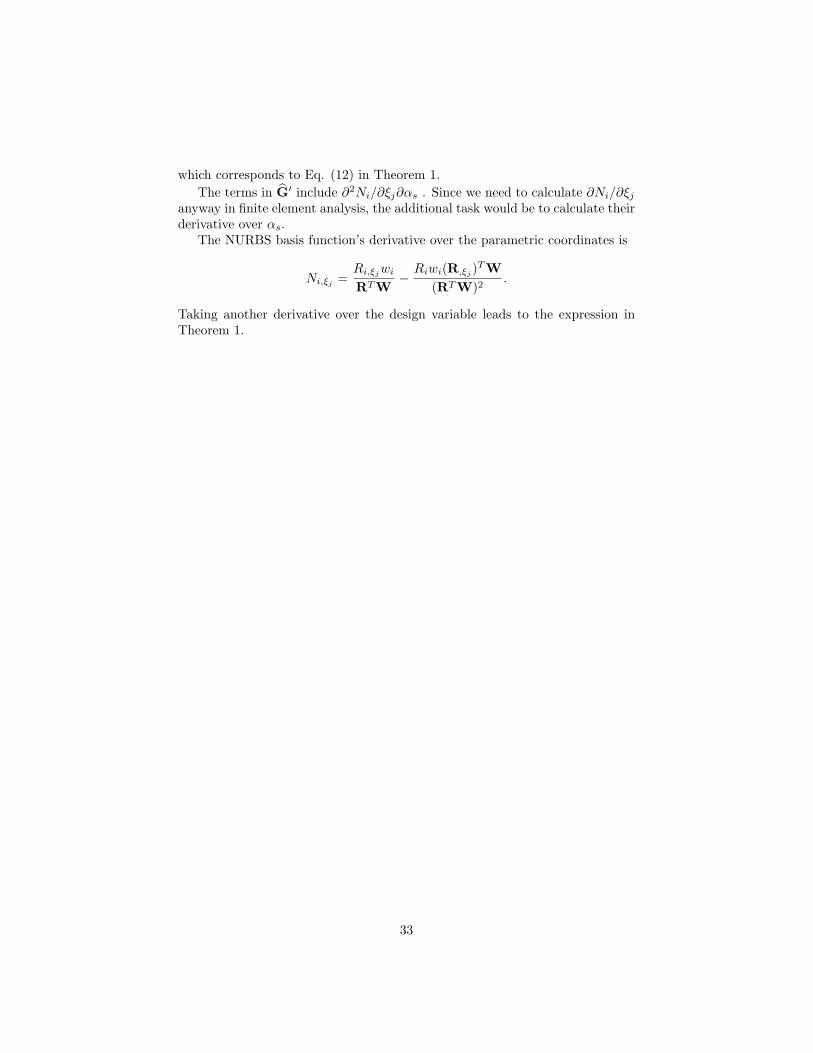
which corresponds to Eq. (12) in Theorem 1.The terms in G′ include ∂2Ni/∂ξj∂αs . Since we need to calculate ∂Ni/∂ξj

anyway in finite element analysis, the additional task would be to calculate theirderivative over αs.

The NURBS basis function’s derivative over the parametric coordinates is

Ni,ξj=Ri,ξj

wi

RTW−Riwi(R,ξj

)TW(RTW)2

.

Taking another derivative over the design variable leads to the expression inTheorem 1.

33

References

[1] Braibant, V., and Fleury, C., 1984. “Shape optimal design using b-splines”.Computer Methods in Applied Mechanics and Engineering, 44, pp. 247 –267.

[2] Samareh, J. A., 1999. A Survey Of Shape Parameterization Techniques.NASA Langley Technical Report.

[3] Hughes, T. J. R., Cottrell, J. A., and Bazilevs, Y., 2005. “Isogeometricanalysis: Cad, finite elements, nurbs, exact geometry and mesh refine-ment”. Computer Methods in Applied Mechanics and Engineering, 194,pp. 4135–4195.

[4] Qian, X., and Dutta, D., 2003. “Physics-based modeling for heterogeneousobjects”. ASME Transactions Journal of Mechanical Design, 125, pp. 416–427.

[5] Yang, P., and Qian, X., 2007. “A b-spline based approach to heterogeneousobject design and analysis”. Computer-Aided Design, 34(2), pp. 95–111.

[6] Schramm, U., and Pilkey, W. W., 1993. “The coupling of geometric de-scriptions and finite elements using nurbs - a study in shape optimization”.Finite Elements in Analysis and Design, 15, pp. 11 – 34.

[7] Choi, J. H., 2002. “Shape design sensitivity analysis and optimization ofgeneral plane arch structures”. Finite Elements in Analysis and Design,32, pp. 119 – 136.

[8] Nadir, W., Kim, I. Y., and de Weck, O. L., 2004. “Structural shape opti-mization considering both performance and manfuacturing cost”. In 10thAIAA/ISSMO Multidisciplinary Analysis and Optimization Conference.

[9] Zhang, X., Rayasam, M., and Subbarayan, G., 2007. “A meshless, compo-sitional approach to shape optimal design”. Computer Methods in AppliedMechanics and Engineering, 196, pp. 2130 – 2146.

[10] Silva, C. A. C., and Bittencourt, M. L., 2007. “Velocity fields using nurbswith distortion control for structural shape optimization”. Struct. Multi-discip. Optim., 33, pp. 147 – 159.

[11] Wall, W. A., Frenzel, M. A., and Cyron, C., 2008. “Isogeometric structuralshape optimization”. Comput. Methods Appl. Mech. Engrg., 197, pp. 2976– 2988.

[12] Cho, S., and Ha, S. H., 2009. “Isogeometric shape design optimization:exact geometry and enhanced sensitivity”. Struct. Multidiscip. Optim.,38, pp. 53 – 70.

34

[13] Poueymirou, D., Tribes, C., and Trepanier, J. Y., 2004. “A nurbs-basedshape optimization method for hydraulic turbine stay vane”. In Proceedingsof the Third International Conference on Computational Fluid Dynamics,ICCFD3, Toronto, 12-16 July 2004, pp. 415 – 421.

[14] Nagy, A. P., Abdalla, M. M., and Gurdal, Z., 2010. “Isogeometric sizingand shape optimization of beam structures”. Computer Methods in AppliedMechanics and Engineering, 199, pp. 1216–1230.

[15] Haftka, R. T., and Gurdal, Z., 1992. Elements of Structural Optimization.Kluwer Academic Publishers.

[16] Brockman, R. A., 1987. “Geometric sensitivity analysis with isoparametricfinite elements”. Com. Appl. Numer. Methods, 3, pp. 495–499.

[17] Haslinger, J., and Makinen, R. A. E., 2003. Introduction to Shape Opti-mization: Theory, Approximation, and Computation. SIAM, Philadelphia.

[18] Christensen, P. W., and Klarbring, A., 2009. An Introduction to StructuralOptimization. Springer.

[19] Piegl, L., and Tiller, W., 1997. The NURBS Book. Springer-Verlag, NewYork.

[20] Fish, J., and Belytschko, T., 2007. A First Course in Finite Elements.John Wilsey and Sons, Ltd.

[21] Svanberg, K., 1987. “The method of moving asymptotes: A new methodfor structural optimization”. International Journal of Numerical Methodsin Engineering, 24, pp. 359 – 373.

[22] Herskovits, J., Dias, G., Santos, G., and Soares, C. M., 2000. “Shapestructural optimization with an interior point nonlinear programming al-gorithm”. Struct. Multidiscip. Optim., 20, pp. 107–115.

[23] Wilke, D., Kok, S., and Groenwold, A., 2006. “A quadratically convergentunstructured remeshing strategy for shape optimization”. Int. J. Numer.Meth. Engrg., 65, pp. 1–17.

[24] Norato, J., Haber, R., Tortorelli, D., and Bendsoe, M. P., 2004. “A geom-etry projection method for shape optimization”. International Journal forNumerical Methods in Engineering, 60, pp. 2289–2312.

[25] Pedersen, P., 2000. “On optimal shapes in materials and structures”. Struc-tural and Multidisciplinary Optimization, 19, pp. 169 – 182.

[26] Bletzinger, K. U., Firl, M., Linhard, J., and Wuchner, R., 2010. “Optimalshapes of mechanically motivated surfaces”. Computer Methods in AppliedMechanics and Engineering, 199, pp. 324 – 333.

35