FRONT-END, BACK-END AND INTEGRATION ISSUES IN VIRTUAL SUPPLY CHAIN DYNAMICS MODELING

Adolfo CRESPO MARQUEZ

Department of Industrial Management, School of Engineering. University of Seville Camino de los Descubrimientos s/n. 41092 Sevilla, SPAIN

Telephone : +34 954 487215; FAX: +34 954 486112 e-mail: adolfo.crespo@esi.us.es

ABSTRACT

In this paper we discuss the way in which dynamic modeling can be used to deal with front-end, back-end and integration issues in current high-tech virtual supply chains (SC).

In a first part of the paper we review and propose dynamic modeling options to connect customer value to business targets. This is done by explaining how to characterize target market by formalizing what are often informal but deeply held beliefs about what drives their customers' purchase decisions. We explain how dynamic models may help to connect planned investments to expected improvements in the customer's perception of the product critical attributes and thus increase sales, revenue, and market share. With the same effort we can importantly educate our customer demand forecast, and get a much better input for subsequent integrated supply chain planning models.

In a second part of the paper we review and discuss the operational and financial effectiveness of existing virtual tools used in supply chain integration. We discuss how dynamic modeling may help to obtain a comprehensive model of supply chain integration. A modeling effort that can be used for the analysis of the effectiveness of various levels of integration, as well as for the assessment of the importance of the sequence in which virtual collaboration tools are adopted in supply chain integration.

In a third part of the paper we discuss and explain experiences in modeling different types of supplier contracts to accomplish varying degrees of security and flexibility. We focus our attention on business dynamics based on current best practices in portfolio management, as evidenced by leaders in volatile high-technology businesses. 1. Introduction Front-end supply chain management—understanding and responding to customer needs—has become a critical part of supply chain strategy. A clear reason for that is the current way that demand manifests itself—via the Web, through online marketplaces or in conjunction with partnerships— which fosters smart companies to increase their emphasis on the supply chain’s front-end [1]. Historically, however, supply chain management focused most intently on improving logistics or the back-end of the supply chain. Supply chains are becoming too complex for any one entity to manage in a competitively dominant way. Companies positioned to work efficiently with multiple partners probably will get most of the action. Rapid and “virtual” partnering also will

be key to new supply chain management strategies, with best integrators working together to attain the biggest prizes[1]. To support the process of migration from internal-only to extended supply chains, a great number of software and hardware tools are showing up, allowing collaboration through the entire electronic SC connection. This has lead to the appearance of the virtual factory or “virtual supply chain” concept [13],[19]. Moreover, new sensors and RFID (radio frequency identification) technologies are allowing capturing on line information about the position of every system’s component. A key aspect of this virtual revolution is how to use this huge amount of available information in order to improve global SC management and performance[10]. In the following sections we review current front -end, back-end and integration issues in virtual supply chains. Our idea is to illustrate how dynamic modeling can help to face emerging problems, current challenges of this new virtual SC era. 2. Modeling Front-End issues Business planning, specially in a high-tech environment, is both dynamic and complex, with a critical need for nonlinear, relational input and mathematical rigor. This is especially the case where planners and decision-makers must rely on subjective and potentially biased data [2], and where data sources span across cultures and languages. Relational input is important where projections of both market demand and competitive position are essential inputs to strategy ([3]; [4]). There is simply not a large enough sample of good data to get statistically valid outcomes on the basis of projections from past trends and patterns, nor are there controlled representative data sources, to support correlations or regression analysis. For all these reasons, planners increasingly turn to simulation models to build confidence and consensus in selecting operational investments to improve or protect market share, revenue, and profit for global high-tech businesses. As a first step in the introduction of a model that can meet these needs, let’s summarize the unique characteristics of the high-tech marketplace [5] : − Volatile, uncertain markets with great pressure on managers for near-term market

share and/or financial performance. − Multiple planning dimensions, including technology path, product architecture,

delivery chain, alliances, channels, and services. − Little historical data, due to technology adoption rates, reorganizations, mergers and

acquisitions, globalization, and new channels for order and distribution. − Isolated groups of expert knowledge, each with their own language and systems. − Absence of a single view of the possible impact of an investment, especially when

results are scattered across space and time, well beyond the scope of any single enterprise planning system.

As an example of a model dealing with the issues in this section we will now present a result of numerous planning team dialogues about the way business grows when it offers a valuable product to an existing market1 (See figure 1). By doing so we

1 Please notice that it is not our intention in this paper to show all the exogenous and endogenous factors that condition results over time, and that would be included in the model for a valid simulation.

present our experience with a clear intention to help the reader in this process of modeling, in case she/he is involved in a similar project..

Figure 1. Business planning process sub-models overview. Our modeling original idea has been linking operational investment, conditioned by policy, to business revenue growth over a financial year. In this way, financial constraints are introduced into the model. Obviously, the higher the growth at a reasonable margin, the greater the level of investments that are available for the next year. The model indeed shows diminishing returns over time, depending on a number of factors. Most importantly, the model clearly shows why "doing nothing" is almost never a good decision for a high-tech business, and helps a business that has enjoyed great success in the past to act aggressively to protect its position for continued profit and growth. Incremental investments are represented in this model as completely variable, even though volume ramps up or down would surely affect the return on fixed costs. We do not include a fixed costs component simply because none of the financial or strategic planners among the companies we worked with have done so. Industry practice is to build fixed costs into overhead rates as part of labor, material, and overhead in internal part costs, or priced into purchased parts, and are not visible to our clients nor used by them when they evaluate and compare business plans. The allowable change in spending level corresponds to an expected changed value of specific attributes. Note that the investment cycle is a consequence of corporate policy and regulated periods to report results and commit resources, where external economic

financial model

Marketshare

Sales

Revenue & revenue growth

Profit & profit contribution

Allowable investments

Perception of value perception

Non price attributes perception Purchasing behavior model

Investments model

financial model

Marketshare

& revenue

Perception of value perception

Non price attributes perception Purchasing behavior model

Investments model

Price attributes

cycles and market occur at their own pace. The model recognizes those delays between a change in spending and a resulting improvement in customer value and sales growth. Business planners try to further group their customers in segments within the target market, according to the relative importance the buyers place on one or the other of the attributes that drive their market overall. In a scenario, investing to improve product attributes drives positive change in customer perceptions, which are assumed by business planners to drive each competitor's share in each segment of the overall market, and of course the related financial results. In terms of confirmation and validation, the general model structure that we have depicted was synthesized and refined with commercial and consumer business managers, systems analysts, critical part contract managers, financial executives, and experts in high-tech workforce collaboration. The results are represented by the three sub-models that we show in figure 1. Let us now present each one of these sub-models. The purchasing behavior model presented here was designed by modeling teams, as presented in Figure 2, where a set of important competitors (or competitor proxies, where a proxy defines a competitive strategy, indexed as i in this figure) were considered. Share here represents the percentage of target market segment sales that can be expected to flow to each competitor over a given time period, knowing that all the factors are continuously changing and influencing each other during that time. Overall market size remains exogenous to the model. The purchasing behavior model can then be explained as follows: a purchaser (it could be a consumer, but also a technical or procurement manager) will most likely select a product according to widely -held perceptions about its quality and price attributes. Examples of quality attributes include reliability, ease of purchase, scalability, network friendliness, service availability, and connectivity. Examples of price attributes include rebates, promotional discounts, cost per instance of use, and channel discounts. Once the purchaser establishes these preferences for the products of the different competitors, we can define the baseline perceptions and we can formalize how much each attribute is able to impact on the value provided by the product to the purchaser. We assume that a purchaser in a segment will pay special attention to the attributes of the product most important to that segment. This concept is formalized through an index of elasticity for each price and quality attributes. Each elasticity value is calculated through the model calibration process, and then its value is maintained for the rest of the simulations. Switching costs and other factors may cause customers to be less responsive to changes in some attributes – this is represented in the model as the inherent elasticity of a quality or price attribute in a particula r segment. Once the impact on the value provided by each attribute of the product is calculated, we can formalize an index that compares the value provided by each competitor’s product. Assessment of these indexes is not difficult since customer perception of their products is tracked somehow by most firms [6]. After that, the model simulates behavior for a given business by showing that the model generates correct changes in individual competitor market share for changes in value (relative to the competition), which can be validated by historical data. It is our main assumption that we can thereafter estimate the share by defined segment for each of the competitors by comparing their customer perception indices, and by assessing their presence in the marketplace. Presence of the competitors in the market has to do with their reach in each segment. Market reach can vary from very monopolistic to very competitive, or even an almost non-existent reach

in any segment. Notice how this model can be considered as a simple attraction model [7] based on the hypothesis that a competitor market share is equal to its attraction relative to all others.

Price Impact onValue

InnovationElasticity

Innovation Impacton Value

ICP Index

Quality AttributeBaseline Perception

Category PremiumDegree Index

Quality AttributePerception perCoompetitor

COMPETITOR i AttributePerception Over Time

Presence ofCOMPETITOR i Proxyper Segment and Product

Share

Price AttributePerception per

Competitor

Price AttributeBaseline Perception

COMPETITOR i Price AttributePerception Over Time

Price AttributeElasticity

Figure 2. Original team design of the purchasing behavior model for three competitors.

How does a product and market strategy impact business revenue? How is revenue over time linked to the product’s price attributes and profit? To answer these questions, we use nonfinancial measures as drivers of financial performance indicators, which is an assumption considered in many examples of current research in this area2. We link market share to revenue and profit by reproducing a pro-forma income statement of the business. All of the businesses we worked with require pro forma statements to also show associated market share , with as much back up information about target segments as possible – either as a % goal to be achieved over time that has been set by corporate, or as the assumed result of the planned operational targets tied to business projections. In addition, working with business controllers led us to incorporate sales discounts for channel incentives, cost of sales and tax factors, extending operations targets for individual programs to show front-end investments and contribution to shareholder metrics. To meet corporate planning guidelines, the business case usually has to project market share, revenue, and profit metrics, with details for the next 4 quarters and summary data over three years. In our experience, 2 For instance Ittner and Larcker [8] have shown how for 2.491 customers of telecommunications firms, customer satisfaction indexes could be correlated to revenue levels, retention and revenue changes of the firms over time. They conclude that their results offer qualified support for recent moves to include customer satisfaction indicators in internal performance measurement systems and comp ensation plans [9].

the financial model is conceived by business planners as shown in Figure 3. The list price strategy is influenced by the market share trend of the business. For example, as a matter of pricing policy, a constraint was inserted in one scenario that raised or lowered the list price if market share projections fit defined gain or loss criteria.

List Price

Revenue

Price Decrease

Share

Unit Sales

Potential Customersper Segment

Total PotentialCustomers

Segment Size

Standard Discount

Margin Discount

Price Increase

Share Trend

Cost of Sales

COS factor

Gross Profit <SGA>

Net OperatingProfit

Taxes

Tax Factor

Figure 3. Original team design of the financial model.

Planning and tracking targets throughout the fiscal year means calculating the rate of investment that the business should direct toward a given market opportunity in order to reach its profit goals. How do we set up a policy to determine the rate of spending we can accomplish? What variables should drive decisions about continuing or changing program investments? Where channel strategy requires incentives in the form of discounts and payments, those costs are added to the computation of net sales as a deduction to compute revenue. In many example scenarios that we simulated, we assume that conditions to increase investment in an existing product map closely to changes in the financial variable values. Profit contribution growth is defined as the difference between projected revenue growth, and the sum of the accumulated growth in the other three variables (revenue, cost of sales and taxes). Finally, SGA expenses for the next year are calculated by considering the profit contribution, revenue growth and other factors.

Aditional Investments (AI)

Revenue Growth (Rg)

<Revenue (R)>

COS Growth(Cg)

SGA Growth (SGAg)

Taxes Growth (Tg)

<Taxes (T)>

SGA

Profit Contribution

<Cost of Sales (C)>

Investments ConstraintFactor (ICF)

Figure 4. Original team design of the investments model. The model can be used to set target spending levels by mapping the pro-forma statement ratios, the proposed spending to increase specific attributes, and the expected returns from a strategy specifically engineered to influence a target segment. The investments model in our example, drawn from actual planning scenarios, was represented with the planning teams as shown in Figure 4, where we find a balance control loop that shows how the rate of growth in profit contribution conditions the growth of the SGA expenses, while ICF, Rg and SGAg, limit that growth3. The following are the main conclusions that we could get regarding front end issues by using dynamic modeling in different projects: • When markets are segmented by customer value and buying behavior, decision

makers may use this modeling to compare expected financial returns on alterna tive investments that appeal to some segments more than others. Investments that affect a specific attribute have different implications for each segment, with results for share, revenue, and profit that also reflect external changes in size of that targeted segment and of the market demand overall. Specific investments considered by teams with whom we have done these analyses in the past include: reseller discounts, pricing strategy, one-to-one relationship marketing programs, advertising

3 Again, policy could depend on other variables according to specific business and market conditions. See, for instance, comments about share in 3rd . and 4th. paragraphs of section 2.

to raise target customer awareness, new channel development, new product and technology introductions, introduction of non-branded offerings, forward contracts to secure critical part supply, and collaborative communication backbones for demand and fulfillment chains4.

• We could found and assess initiatives to improve business performance, directed toward specific solution attributes, for instance: Quality attributes were improved by investments to improve features, performance, power requirements, footprint size, integration, customization, delivery, localization, scalability, interoperability, quality, channels, and alliances; Price attributes were improved by investments in aggressive sourcing, parts availability, risk management, order and forecast management, channel incentives, discounts, rebates, advertising, web-based collaborative infrastructure, and synchronized product upgrades.

• The modeling effort could help to confirm the critical assumption that your planned spending will indeed increase customer perception and impact sales as you expect.

• In addition to mining existing market research, our planners tended to gain confidence through immediate action guided by the model used as a decision support system, with a rapid "pilot", limited in scope and carefully observed to measure and confirm perception and response.

3. Virtual integration issues modeling

Internet based information systems offer a great opportunity to improve supply chain management (SCM). The new Internet based e-collaboration tools allow us to integrate multiple organizations and facilitate the flow of information from any one source in a supply chain (SC) to all SC partners [10]. These low cost tools use the emerging standards for data exchange such as XML (extended markup language). While the collaboration and synchronization of all SC participants, both within and outside the firm, is now feasible, such supply chain integration needs to be carefully studied in order to improve its implementation.

Issues involved in supply chain integration have been studied in the literature

from various perspectives. Gavirneni et al. [11] analyzed the benefits of the integration of information flows in a supply chain for a capacitated two-echelon SC . Chen [12] studied the importance of having access to accurate demand information for the SC upstream members. The benefits of integrating the SC and diminishing the demand oscillation transmission along the chain (the bullwhip effect) has been explored by Towill et al., [13] and Chen et al. [14]. These studies show that information sharing can significantly impact the SC performance. However, information sharing is only a subset of the supply chain. Researchers agree that the SC planning and control activities are also included in integration [15].

4 Notice how in many high-tech sectors like telecom infrastructure or medium business manufacturing, the end "product" is a solution, i.e. multiple component products with different cost structures bundled for this market to meet this set of attributes. Financial targets usually represent product businesses selling into numerous markets, where go-t o-market, sales, service, and channel investments are treated as programs, charged with achieving specific market objectives. Although current financial data usually comes to us as product business targets, most critical investment decisions must also consider the impact of changes in attributes and customer perception of value for a solution which will determine its success or failure.

When considering the planning and control activities, the effectiveness of SC integration may depend on the sequence of tools used in SC integration. However, this issue has received only a scant attention in the existing literature. Stevens [16] presented an integration model with four phases: baseline, internal functional integration, integrating supply and demand along the company’s own chain, and full supply chain integration. Hewitt [17] expanded Stevens’ model with a fifth phase that would be dedicated to better administration and re -engineering of the global business processes, pursuing the total effectiveness and efficiency of those processes. Scott and Westbrook [18] suggested a three phase model to reach an integrated supply chain: an initial “phase of study” where lead times and inventory levels are analyzed for potential improvements; a “positioning phase” to identify new opportunities emerging as a consequence of collaboration activities among the members of the chain; and an “action phase” to put previous plans into effect. Towill et al. [13] present a SC integration approach that is similar to the one presented by Scott and Westbrook [18]. In their work, Towill et al. [13] also use operations management principles to reduce the amplification of the demand signal along the chain when the integration is produced.

Bowersox [19] suggests that the creation of time and location benefits not only

requires sharing the information to allow suitable business agreements with that purpose, but also requires the existe nce of a suitable environment for financial transactions. The integration of SC financial flows is also becoming a common topic in literature, because of its impact on the entire supply chain performance. Automated freight payment software is available to pre-audit, summarize, batch, and pay carriers by electronic checks on a scheduled basis [20]. There is evidence [21] that the use of information integration in conjunction with buyers’ and sellers’ banks to transfer funds can improve cash flow and reinforce the “partnering” relationship between the parties in the supply chain. Further, in many supply chains, credit provision is a key factor in supplier choice among distributors and their customers [22]. Suppliers often finance their customers’ transactions through the extension of free credit. Clearly, cash flow is affected by the terms of sale, and buying and selling companies often have a different capital cost, which raises the opportunity of improving supply chain performance by having the company with the lowest cost of capital own goods for as long a period as possible [10]. Many times, a financial organization can provide the “banking function” financing shipments by purchasing those receivables, at a discount, eliminating the seller’s extension of credit terms and their incurring payment delays from letters of credit [23].

The review of the existing SC integration literature reveals that there is no

comprehensive SC integration model. We have been deeply involved in research to present a comprehensive supply chain model that could be used to determine the operational and financial benefits of various levels of supply chain integration using e-collaboration tools. Such a SC model would also enable us to analyze the impact of partial integration effor ts. Let us see then how to characterize and model the types of information sharing and collaboration steps.

The possible information for sharing include inventory, sales, demand forecast, order status, product planning, logistics, production schedule, etc., and can be summarized into three types: product information, customer demand and transaction information, and inventory information.

• Product information

Original exchange of product information among the supply chain partners was done by paperwork, such as paper catalog, fax, etc. The problems caused by this include delays in information sharing and miscommunications among the trading partners. To add the product information into its information systems, a retailer has to re-enter the data, which may or may not come along with the product, manually. Then, to keep the data updated is an even harder task. For example, if some information has been changed since its last release, all the retailers in the industry (if they are lucky enough to) have to check the data individually. According to UCCnet, 30 percent of data exchanged between suppliers and retailers does not match up due to the inefficiencies of manual data entry and convoluted processes (http://www.uccnet.org). This is an enormous problem for the industry, because bad data translates into a bad understanding of what retailers actually have on their shelves and what suppliers actually have in their warehouses. Bad data translates directly into huge costs, missed revenues, and, often enough, end-user dissatisfaction as, for example, when shoppers find that heavily advertised products are not in stock. According to a case study conducted by Vista Technology Group (a CPG software provider), Shaw's (a supermarket chain that has been serving New Englanders for over 140 years) manual, paper-based new item introduction process had no less than 17 steps (http://line56.com/articles/default.asp?NewsID=2885). This meant a labyrinthine, time-consuming internal process; it also meant that suppliers' product upda tes -- even something as simple as changing the size of a can of tomatoes -- had to go through the same manual, error-prone procedure before Shaw's could get the data in its systems.

EDI was first introduced for data interchange. Although EDI was originally designed to be a means to process transactions, it has been extended to facilitate sharing of some information like POS and on-hand inventory [24]. However, EDI has its own limitations. In addition, EDI does not verify data accurateness; it just transmits the data--“Garbage in, garbage out”.

• Customer Demand and Transaction Information

Customer demand and transaction information serves as a critical source of information about future business, and is directly used for demand forecasting, manufacturing schedule, transportation planning, etc.

Lee and Whang [25] provide an example of transaction information sharing in

Seven-Eleven-Japan’s (SEJ). In SEJ case, POS data are transmitted to SEJ headquarters, wholesalers, and manufacturers to monitor stocking levels, shelf space organization, merchandizing, and new product development.

The recent developed Collaborative Forecasting and Replenishment (CFAR) is

a new inter-organizational system that enables retailers and manufacturers to forecast demand and schedule production jointly [26].

• Inventory Information

Inventory information, including inventory status and inventory decision models, directly affects the amount of order placed to the immediate upper stream supply chain partners. However, inventory information seems to be more sensitive than customer demand and transaction information, and the trading partners are less willing to share it. For example, manufacturers may not be willing to divulge their true inventory situation or may portray false inventory levels to discourage competitors from producing additional products or building additional capacities and suppliers may use inventory and sales data to get a better bargaining leverage.

In practice, sharing of inventory information is implemented in different forms.

CRP (Continuous Replenishment Programs) or Vendor-Managed Inventory (VMI) is a practice often employed by two neighboring partners in a supply chain. In a typical CRP relationship, the buyer shares its inventory data with vendor and asks the vendor to manage his inventory within guidelines. Wal-Mart’s Retail Link program [27] and Apple-Fritz Supplier Hub [25] are good examples of sharing inventory information.

VMI system let the manufacturer maintain the retailer’s inventory levels. The

manufacturer has access to the retailer’s inventory data and is responsible for generating purchase orders. (http://www.vendormanagedinventory.com/definition.htm) The major difference between VMI and regular information sharing is that under VMI, the manufacturer generates the purchase order, not the retailers.

• Collaboration steps The steps of collaboration are ways or processes that firms follow to collaborate

with their partners. The departure point of our supply chain will be a lack of collaboration, “Non Collaborative (NC)” SC, meaning that the trading partners does not share critical information (e.g. they only transfer information about products, orders and orders state, and exclusively between each supplier-customer relationship). Time delays exist in receiving and processing orders, as well as in knowing the real inventory levels.

In a first improvement step, “Collaborative Forecasting (CF)”, offers the

possibility to speed up the information about end customer demand along the chain, enables partners to make consensus -based forecasting and allows the orders in the supply chain to be visible in real time, and processed accordingly. The goal of consensus based forecasting is to consolidate the various forecasts into a common time series to be used for further planning. Business partners can view each other’s forecasts, make changes and agree on a consensus -based forecast using just an Internet Browser.

In a second improvement step, “Collaborative Planning (CP)”, allows the supply

chain members to gain access to additional information that they do not control, and use it in their planning process. In this paper we assumed that firms gain access to additional information about finished good inventories (FGI) and work in process inventory (WIP) of downstream supply chain members. This means that, CP is an aggregate of collaborative forecasting and collaborative inventory, or VMI.

We first assume this sequence of steps to improve the performance of the supply chain through collaboration. A reason for this is that analysts agree that VMI has been successful in many cases, but inaccurate forecasts and undependable shipments have been major obstacles to higher performance. When collaboration does not exist in the supply chain, an inventory manager only has operative information about the order placed by its direct downstream partner(s). The desired order rate to the previous firm depends on the local firm forecast and on local inventor ies, see for instance how we have modeled this forecast in equation (1) (from [28] ), where desired production orders from each firm (equation 2) are computed by means of an anchoring and adjustment heuristic [29] with fractional adjustments coefficients ( Sβ ,

SLβ ) for the FGI and the WIP, not allowing negative values of quantity to request (like in [30]), and including in the equation the backlog of the upstream Firm at the end of the last period t-1 . The reason for this is to enable immediate shipments (zero expected backlogs under normal conditions). Further, each node includes its last period backlog as part of the desired shipments in the next period t. Therefore the backlog will be fulfilled as soon as on-hand inventory becomes available.

i

t

ii

t

ii

t D 1

^1

1

^

)1( −+− −+= µµ αα , ii ∀≤< ,10 α trading partner (1)

)0,)()(( 1

1

^^^−−−−+−+= i

t

i

t

ii

tSL

i

t

ii

tS

i

t

i

t BPLYssMaxOP µβµβµ (2)

where:

itP : pipeline from Firm i to the next Firm i+1 , (includes work in

process inventory in the Firm plus the inventory of parts in transportation to the warehouse of finished materials) in period t

1+itOP : orders placed, of material units, by the Firm i+1 in period t, 1+i

tD : orders of material units, received in the Firm i in period t, itB 1− : existing backlog of orders in Firm i in t-1 ,

α i : firm i forecast smoothing factor,

Sβ : fractional adjustment coefficient for the on-hand inventory,

SLβ : fractional adjustment coefficient for the pipeline inventory, i

t

^

µ : forecast of firm i in period t, iL : lead time for a material unit in the pipeline to arrive to the

inventory of finished materials

Changes to introduce in order to model a collaborative forecasting (CF) structure are as follows: In this way of collaboration, trading partners share the end customer’s information in order to obtain a consensus and to use the same forecast to

place their orders. The chain now collaborates on meeting end-customer demand, discusses issues and sales expectations (on a time period /weekly basis). Therefore equation (1) is replaced with the following formulation (3):

nin

t

i

t ,..1,^^

=∀= µµ , where i represents the trading partners (3)

This is,

n

t

ncustt

ni

t D 1

^

1

^

)1( −− −+= µµ αα with in ∀≤< ,10 α , (4)

and custtD 1− is the last time period demand for the end customer of the chain. Once the

new firm forecast is obtained, the orders are calculated as in (2). In this way the individual forecast and orders information is known in real time along the chain.

In case we have to model the collaborative planning(CP) structure we ha ve to

consider that the collaborative partnership extends to collaborative inventories and ordering in the entire network. That means that there is no need for local forecasts, all supply chain partners will be provided through the internet with real-time forecast, demand information, and they will have visibility to inventory and capacity utilization along the chain. With that purpose, in this “full” collaborative structure is assuming that an “information backbone” (common shared information system) has been totally developed in the chain. In practice, this is where VMI (Vendor-Managed Inventory) and CFAR (Collaborative Forecasting and Replenishment) fit in.

For the Collaborative Forecasting and Replenishment (3) and (4) are still applicable, but the following formulation (5 & 6) is introduced, replacing (2)):

)0,)()(( 1

1

^^i

t

i

t

i

t

i

t

ii

t

i

t

i

t

i

tibBYPLssMaxOP +−+−++= −

−µµ (5)

Where itib is a variable expressing the information provided to the Firm i

through the information backbone in time t:

11111^

)()( +++++ ++−+= i

t

i

t

i

t

iii

t

i

tibYPLssib µ (6)

We have proposed a sequence (Figure 5) to improve the performance of the SC

through a gradual increment in the collaboration. Further important analysis regarding this point could be done. That is, exploring and checking what would happen if in the first step, the Vendor-Managed Inventory process is used by firms, and then, Collaborative Forecasting is added. Figure 5 illustrates the sequence proposed in order to expand the collaboration, and the alternative sequence.

The following are the main conclusions that we could get regarding supply chain integration by using dynamic modeling in different projects: • It is certain that, the gradual increments of the information sharing, produces

positive increases on the local and global performance of the SC. • To carry out this new practices, we could find out that we should first address the

issue of collaborative demand forecasting (implementing the collaborative forecasting), which allows us to reach a higher efficiency increment than the vendor-managed inventory practice, this is, more uniform behavior of the inventories along the chain and therefore smaller average cash requirements, while both practices offer similar service levels.

• From the collaborative planning, the SC can benefit from the complete visibility of the total materials flow along the chain. This produces smallest movement and storage of materials along the chain, enabling the ordering policies to adjust new customer requirements earlier, and with more efficient inventory administration (less inventory investment and cost to reach a target service level) along the chain.

• Furthermore, collaborative planning leads to the prompt stability in critical variables, to the best service levels to end customers, the highest throughput.

• When e-collaboration tools are implemented in the SCM, each upstream supplier has a stable sale and each downstream customer orders stable amount of products, in spite of the communication of the information has to go through multiple intermediaries between the consumers and the raw material sources. The processes are more agile, the costs are more favorable and the service to the end customer, the best.

Figure 5. Steps in the Expansion of the Collaboration and Sharing Information Scenarios in the Supply Chain (from [31])

CP

Basic Structure

Product,Orders

Non-CollaborativeNon-Collaborative

(NC)(NC)

S0

Information shared:

S1

Scenario 1

S1

VMI

VMI: Vendor-Managed Inventory

CF

CF: Collaborative Forecasting

CP

CP: Collaborative Planning

Scenario 2

S2

Scenario 0

Product,Orders,

Information shared:

Product,Orders,

Information shared:

Product,Orders,

Information shared:

Inventories

Forecast

Inventories,

Forecast

Sequence 1:Proposed

Sequence 2: Alternative

• financial collaboration modeling One of the most important responsibilities of the treasurers of different nodes of the supply chain is the management of the sources and uses of funds. While making sure that cash is available to meet short-term needs, such as payrolls and invoice payments to the other nodes, treasurers must plan for strategic funds management to facilitate long-term growth via capital expansion or acquisition.

AccountsPayable

(Py)

AccountsReceivable (R)

% ContributionMargin (Cm)

Interest Rate

MaterialPurchases (Mpu)

MaterialsPayments (Mpy)

Sales Revenue(Sr)

SalesCollections (Sc)

InventoriesValue (IV)

Cost of PurchasedMaterial (Cpm)

Cost of Sales(Cos)

Production/ShippingCost (Cps)

InventoryIncrease in

Increase inReceivables

Reduction inPayables

Cash of theNode (C)

Current income(Ci)

Increases inWorking Capital

(Iwc)

Max BankCredit (Mb)

Available BankCredit (Ab)

Bank CreditUsed

Financialexpenses (Fe)

Cumulative Income (Cci)

Max Order RateFinancial Constraint

(Mor)

Figure 6. Overview of the financial model through a

“stock and flow” diagram, and for a generic node of the supply chain (from [32])

The tool for this kind of analysis is the “sources and uses of funds statement” that may be estimated for any interval of time. The change in the SC node’s cash position will be defined as the difference between sources and uses of funds5 (the reader is referred to [33], pp 21-25, for the implications of the elements of this financial statement). Since there is a multiplicity of factors impacting a firm’s cash position, we have paid special attention to those aspects that are related to the income from operations, and to the increments of the net working capital (an overview of this financial model is shown in Figure 6 where for sake of simplifying the presenta tion, we have not included depreciation and other non-stationary costs thus making the inflow

5 Another possibility would be to define increases in cash balances as a use of funds and decreases as a source. Then total sources would have to equal total uses. Normally, sources and uses statements adopt this procedure.

equal to its current income). In this context, we have to remark the importance of inventory, that is frequently the largest asset in the SC and source of controllable costs [34]. Taking into account all previous considerations, we have built several system dynamics based simulation models and used them to study the impact of various levels of supply chain integration in different case studies. The following are the main conclusions that we could get regarding supply chain financial integration by using dynamic modeling: • In some cases we found that the implementation of e-collaboration tools to do local

planning using global SC inventories data when each node is producing its own forecast could lead to significant increases in inventory and decreases in income, especially where nodes are not financially constrained.

• Our computational results also showed that it is risky to install e-collaboration tools for electronic payment when collaborative forecasting is not in place in the SC. Decreases in financial constraints could lead to unnecessary increase in inventories without improving SC performance.

• Local financial constraints can heavily impact the operational and financial performance of the entire supply chain. At times, this impact could be very close to the one produced by a global financial constraint at all the nodes of the SC. Therefore, helping the weakest financial node of the chain was found to be a main concern of the SC engineers and analysts, this aspect should never be treated as a SC local issue.

4. Modeling Back-End issues

Creating and managing contract structures for supplier management is necessary in order to assess the capacity of the organization for high performance [35]. This specialization is a must for an effective structural design of the organization as a whole. This expansion of the purchasing role is required to secure an adequate supply in global markets, while protecting profit margins under pressure from global competition. Giunipero and Brand [36] developed a framework describing the stages of the evolution towards supply chain management (SCM), and how procurement would change within that framework. They defined four levels of development of the purchasing role: 1) Traditional, emphasizing vendor selection and lowest possible pr ice; 2) Partnership/relational, building closer relations with a supplier to reduce total cost and minimize risk in an atmosphere of trust; 3) Operational, (material logistics management), coordinating material and information flows to improve quality, inventory levels, and overall cost; 4) Strategic, (integrated value added), applying flexible business processes to a given situation, and thereby achieving speed, flexibility, and competitive advantage in the marketplace.

In large multinational companies, the current movement to consolidate supply

chain management across business units in geographic areas, and the integration of product units into customer-facing solution businesses by target market, offer new possibilities for strategic sourcing and a contract portfolio. The idea is to create consistent relationships between the suppliers of a commodity-type part and the various procurement organizations, locking in competitive prices for the same contractual terms, tracking different product part specifications to a corporate-wide technology

strategy [37] , etc. Competitive procurement strategies [38] focus on the buyer’s intrinsic bargaining power, which allows buyers to leverage purchasing on a global scale, minimize internal costs, and improve the company’s competitive advantage. In this context, global sourcing [39] is a fundamental corporate strategy aimed at maximizing the utilization of worldwide material resources.

Some industrial sectors, like high-technology, face volatility from unpredictable

demand and very short product and technology life cycles. Organizations within these sectors develop flexible procurement strategies to deal with this uncertainty. The numbers of suppliers available, plus a range of tiered contract structures, are critical to meeting this need for flexibility. In such sectors, worldwide capacity for certain parts may be very limited relative to demand at any stage of the commodity’s technology life cycle. The global supply is also vulnerable to unexpected events, (such as natural disasters, social-political changes, terrorism, and economic disasters) that may create scarce worldwide supplies of certain commodity parts. When products are strategically important for the company, multiple sourcing of strategic parts is used to decrease exposure to potential loss, but in addition companies are now combining types of supplier contracts to ensure availability of supply at a competitive cost.

The use of multiple sourcing is assumed to diminish the risk of delays or failure

on the part of just one supplier [40] , and may also encourage their performance as regards delivery and quality [41]. Other factors influencing multiple source are economics, geography, organizational policy and buyer inertia. Multiple sourcing should be adopted as a procurement strategy in those cases where items are critical in the production process and which incur high cost if the production lines are stopped [42].Where supplier contracts are structured on volume discounts, higher part prices might be charged when demand volume is allocated to multiple sources, but that increase can be seen as an insurance against the higher total cost of stopped production [43].

In researching how to manage and value a portfolio of supplier contracts, we have modeled the strategic parts procurement system with a system dynamic model to illuminate the dynamics of the procurement process, and to assess the value of a contract portfolio within this process. Different strategy options for supplier contracts portfolio will face this problem, allowing the company to gain market and price positions, to ensure required customer service levels, and to diversify and secure source in times of scarcity.

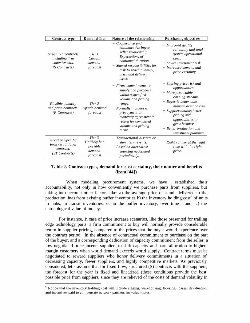
After our involvement in several procurement risk management projects, we

present in table 2, a vision of the most popular contract types found within the high-tech industry, their purpose, and the way in which the relationships are established between the parties.

Contract type Demand Tier Nature of the relationship Purchasing objectives

Structured contracts including firm commitments. (S Contracts)

Tier 1 Certain demand forecast

− Cooperative and collaborative buyer seller relationship. Expectations of continued duration.

− Shared responsibilities for task to reach quantity, price and delivery terms.

− Improved quality, reliability and total system operational cost..

− Lower investment risk. − Increased demand and

price certainty.

Flexible quantity and price contracts.

(F Contracts)

Tier 2 Upside demand

forecast

− Firms commitments to supply and purchase within a specified volume and pricing range.

− Normally includes a prepayment or monetary agreement in return for committed volume and pricing terms

− Sharing price risk and opportunities.

− More predictable earning streams.

− Buyer is better able manage demand risk

− Supplier obtains better pricing and opportunities to grow business.

− Better production and investment planning.

Short or Specific term / traditional

contract. (ST Contracts)

Tier 3 Unlikely but

possible demand forecast

− Transactional, discrete or short term events.

− Based on alternative sourcing negotiated periodically.

− Right volume at the right time with the right price.

Table 2. Contract types, demand forecast certainty, their nature and benefits (from [44]).

When modeling procurement systems , we have established the ir accountability, not only in how conveniently we purchase parts from suppliers, but taking into account other factors like: a) the average price of a unit delivered to the production lines from existing buffer inventories b) the inventory holding cost6 of units in hubs, in transit inventories, or in the buffer inventory, over time ; and c) the chronological value of money.

For instance, in case of price increase scenarios, like those presented for trailing edge technology parts, a firm commitment to buy will normally provide considerable return in supplier pricing, compared to the prices that the buyer would experience over the contract period. In the absence of contractual commitment to purchase on the part of the buyer, and a corresponding dedication of capacity commitment from the seller, a low negotiated price incents suppliers to shift capacity and parts allocation to higher-margin customers when world demand exceeds world supply. Contract terms must be negotiated to reward suppliers who honor delivery commitments in a situation of decreasing capacity, fewer suppliers, and highly competitive markets. As previously considered, let’s assume that for fixed flow, structured (S) contracts with the suppliers, the forecast for the year is fixed and linearized (these conditions provide the best possible price from suppliers, since they are relieved of the costs of demand volatility in 6 Notice that the inventory holding cost will include staging, warehousing, flooring, losses, devaluation, and incentives paid to compensate network partners for value losses.

their inventory levels and capacity utilization through the contract horizon, the terms could further discount the unit price for early payment). The overriding purpose of structured contracts is of course to secure capacity and protect profit margins in the face of almost certain inability of world capacity to meet expected demand, and corresponding increasing prices. The supplier who negotiates a flexible flow (F) type of contract experiences volatility in demand, and not only as a consequence of the final product market volatility, but also as a consequence of the supply chain structure and corresponding bullwhip associated to it.

In order to structure the contracts with the suppliers (S and F), a valuation

procedure can be to establish the deal as a series of forward contracts for each delivery period (roughly speaking, a forward contract is a contract to buy or sell at a price that stays fixed for the life of the contract), and then use the conventional valuation approaches for their financial assessment7 [45]. If we do so, current price will be used as a basis (BP, in US$) for the valuation since the product is considered to be purchased at present (we would use current price for a quantity of parts corresponding to the total annual purchase), discounted based on expected (forecast) delivery, but deferring payments until the time of delivery although contract would be binding. The real purchase cost of a unit of critical part will take into account the cost of borrowing 8 the money (r, in %) until the part is delivered by the supplier, plus the usual net payment terms the procurement system has with its suppliers (PT, in weeks). If we consider that all deliveries for the year were paid upfront, borrowing cost9 should be calculated for each part delivery period (t, in weeks). Delivery price for a part delivered n period t under a fle xible contract (DPfc) would be then calculated10 according to (7), which is replacing (1), after articulating the forward contract: DPfct = f(t,BP, PT, r)= BPer(t+PT) (7)

Notice how, by paying the marginal amount BP (er(t+PT)-1), we limit the cash investment and price risk in the purchase of a part in period t.

Another contractual possibility with suppliers that we could model is based on commodity options. A commodity option is an option to buy (call option) a fixed quantity of a specified commodity at a fixed time in the future and at a fixed price. It differs from a security option in that it can’t be exercised before the fixed future date. Thus is an “European Option” rather than an “American Option” [45]. A commodity option differs from a forward contract because the holder of the option can choose whether or not he wants to buy the commodity at the specified price. Notice that with the forward contract he has no choice: he must buy it, even if the spot price at the time of the transaction is lower than the price he pays.

Taking into account all previous considerations, we have built several system dynamics based simulation models and used them to study the impact of various type of

7 The value of a forward contract is the difference between the futures price and the forward contract price, discounted to the present at the short -term interest rate. 8 As “cost of borrowing”, the cost of capital could also be used. 9 Notice how the borrowing cost for a year is also the real value of having the supplier to hold inventory or capacity during that period. 10 Assuming continuous compounding.

relationship with a supplier in different case studies. The following are the main conclusions that we could get:

• Each type of relationship with a supplier will pursue a different objective, and will

have some different trade-off implications that we have to acknowledge, and that will lead to the consideration of certain types of policy and managerial practices for each type of supplier.

• Modeling the tiered approach allowed, besides protecting from risk, the selection and implementation of convenient deals with each specific supplier, protecting the supplier if needed, aligning him to serve specific market needs, or market strategies.

• Specifically, our models could simulate the tradeoffs available to managers in the various contract structures, in this sense, it is very helpful to understand the implications of the different contract parameters, when markets conditions may change, and for metrics selected by the decision maker.

• These models are also suitable to simulate the combined impact of a portfolio as a whole, in the context of the overall supplier relationship.

5. Conclusions We have explored the opportunity to use dynamic modeling as a tool to assess different current issues in the front-end and back-end of the supply chain, as well as in issues related to supply chain virtual integration. Regarding front-end issues we have explained how dynamic modeling could greatly improve analysis of go-to-market strategies, integrating customer knowledge with simulations to analyze spending trade -offs in features, services, support, integration, channel incentives, pricing, and advertising. The models developed became a powerful DSS tool offering the opportunity to compare strategies for a segmented market, under different scenarios, with customized metrics. Regarding SC integration we review how dynamic modeling could contribute to obtain a comprehensive model to study the operational and financial benefits of using various e-collaboration tools. Simulation could be used to study the impact of various levels of supply chain integration. Experience could clearly show the potential improvements of the integration by using Internet tools for SC collaboration. The sequence of implementing this new technology was found to be very relevant. Concerning back-end issues, this modeling approach and framework could be used for the proactive design of the contracts with suppliers , and for the analysis of the problem from both, the supplier and buyer perspectives. A full valuation of inventory and related carrying costs, inclusion of accepted predictive statistical tools, and tracking the cost of capital in valuing cash flows over time, all allow these models to fully support the creation and management of options contracts in lieu of forward contract structures for flexible demand management.

6. References

• Front-end [1] David L. Anderson and Allen J. Delattre 2002.Five Predictions That Will Make

You Rethink Your Supply Chain. Supply Chain Management Review. September/October.

[2] Hogarth R.M., Makridakis S. 1981. Forecasting and Planning: An evaluation. Management Science. 27(2), 115-138.

[3] Day G.S. 1990. Market driven strategy: Processes for creating value. The Free Press. New York, NY.

[4] Schnaars S.P. 1991. Marketing Strategy: A Customer-Driven Approach. The Free Press. New York, NY.

[5] Crespo Marquez A. & Blanchar C. 2004. A Decision Support System (Dss) For Evaluating Operations Investments In High-Technology Business. Working Paper. Department of Industrial management. School of Engineering. University of Seville.

[6] Ross J. and Georgoff D.. 1991. A Survey of Productive and Quality Issues in manufacturing. The State of the Industry. Industrial Management. Jan-Feb. 3-5, 22-25.

[7] Carpenter G.S., Cooper L.G., Hanssens D.M. and Midgley D.F. 1998. Modeling Asymmetric Competition. Marketing Science. 7(4). 393-412.

[8] Ittner C.D. and Larcker D.F.1998. Are Nonfinancial Measures Leading Indicators of Financial Performance? An Analysis of Customer Satisfaction. Journal of Accounting Research. 36(suppplement). 1-31.

[9] Kaplan R.S. and Norton D.P. 1996. The Balanced Scorecard. Boston. Harvard University Press. 1996.

• Integration

[10] Mentzer, J. T. 2001. Supply chain management. Sage Publications, Inc. 306-319. [11] Gavirneni, S., R. Kapuscinski and S. Tayur. 1999. Value of Information in

Capacitated Supply Chains. From Quantitative Models for Supply Chain Management. Eds. Magazine, M. J., Tayur, S. and Ganeshan, R. Kluwer. Cambridge.

[12] Chen, F., 1999. Decentralized supply chains subject to information delays. Management Science, 45(8), 1076-1090.

[13] Towill, D. R., Naim, N.M., Wikner, J., 1992. Industrial dynamics simulation models in the design of supply chains. International Journal of Physical Distribution and Logistics Management. 22. 3-13.

[14] Chen, F., Drezner, Z., Ryan, J. K., Simichi-Levy, D. 1999. The bullwhip effect: managerial insights on the impact of forecasting and information variability in a supply chain. Quantitative models for supply chain management. International Series in Operations Research & Management Science, 17, Ed. Mayur. Ganeshan & Magazine. 419-439.

[15] Jones, T. C. and D. W. Riley. 1985. Using Inventory for Competitive Advantage through Supply Chain Management. International Journal of Physical Distribution and Materials Management 15. 16-26.

[16] Stevens, G. C. 1989. Integrating the Supply Chain. International Journal of Physical Distribution and Materials Management.19. 3-8.

[17] Hewitt, F. 1994. Supply Chain Redesign. The International Journal of Logistics Management. 5 (2). 1-9.

[18] Scott, C., Westbrook R., 1991. New strategic tools for supply chain management. International Journal of Physical Distribution and Logistics Management. 21(1), 23-33.

[19] Bowersox, D.J., 1997. Integrated supply chain management: a strategic imperative, presented at the Council of Logistics Management 1997 Annual Conference, 5-8 October, Chicago, IL.

[20] Cooke, J. A., 1996. The check in the computer. Logistic Management. 32(12), 49-52.

[21] 0rr, B., 1996. EDI: Banker’s ticket to electronic commerce. ABA Banking Journal, 88(5), 64-70.

[22] Neal, B. 1994. Springing the distribution credit trap. Credit Management. December. 31-35.

[23] Davis, K. 1998. Cash forwarding expands business for University Medical Products. Business Credit. 100(2). 10-12.

[24] Sokol, P. 1995. From EDI to Electronic Commerce. McGraw-Hill Inc. [25] Lee, H., and W. Whang. 1998. Information Sharing in a Supply Chain. Research

paper No. 1549, Stanford University. [26] Raghunathan, S. 1999. Interorganizational Collaborative Forecasting and

Replenishment Systems and Supply Chain Implications. Decision Sciences. 30(4): 1053-1071.

[27] Gill, P. and J. Abend. 1997. Wal-Mart: The Supply Chain Heavyweight Champ. Supply Chain Management Review. 1(1). 8-16.

[28] Makridakis, S., S. Wheelwright and R. Hyndman. 1998. Forecasting methods and Applications. John Wiley and Sons.

[29] Tversky, A., and D. Kahneman. 1974. Judgement under Uncertainty. Heuristics and Biases. Science.185. 1124-1131.

[30] Sterman, J. D. 1989. Modeling Managerial Behavior: Misperceptions of Feedback in a Dynamic Decision Making Experiment. Management Science. 35(3). 321-339.

[31] Rubiano Ovalle O. & Crespo Marquez A. 2003. A simulation study to assess the impact of Internet in the supply chain management. Journal of Purchasing and Supply Management. 9(4) .151-165.

[32] Crespo Marquez A., Bianchi C., Gupta J.N.D. 2004.Supply Chain Integration Through E-Collaboration Tools. To Appear In The European Journal Of Operations Research. (in print).

[33] Weston, J. F., Copeland T. E., 1989. Managerial finance (Eight Edition). The Dryden Press, Chicago, IL

[34] Rockhold, S., Lee, H., Hall R., 1998. Strategic alignment of a global supply chain for business success. POMS Series in Technology and Operations Management. Vol.1, Global Supply Chain and Technology Management. 16-29.

• Back-end

[35] Scott, W.R. 1987. Organisation: Rational, Natural and Open Systems. 2nd.

Edition. Prentice-Hall International Edition, Englewood Cliffs, NJ. [36] Giunipero, L., Brand R.R. 1996. Purchasing’s role in supply chain management.

The International Journal of Logistics Management. 7(1). 29-38.

[37] Nellore, R., Motwani, J. 1999. Procurement commodity structures: issues, lessons and contributions. European Journal of Purchasing and Supply Management. 5. 157-166.

[38] Spekman, R.E. 1988. A strategic approach to procurement planning. Journal of Purchasing and Materials Management. 25th Anniversary. 4-8.

[39] Arnold, U. 1989. Global sourcing- an indispensable element in worldwide competition. Management International Review. 29(4). 20.

[40] Min, H., Galle. W.P. 1991. International purchasing strategies of multinational U.S. firms. International Journal of Purchasing and Materials Management. Summer. 9-18.

[41] Carr, C.H., Truesdale, T.A. 1992. Lessons from Nissan’s British suppliers. International Journal of Operation and Production Management. 12(2). 55.

[42] Quayle, M. 1998. Industrial procurement: factors affecting sourcing decisions. European Journal of Purchasing and Supply Management. 4. 199-205.

[43] Asanuma, B. 1985. The organisation of parts suplí in the Japanese automotive industry. Japanese Economic Studies. 15. 32-53.

[44] Crespo Marquez A., Blanchar C. 2004. The procurement of strategic parts. Analysis of a portfolio of contracts with suppliers using a system dynamics simulation model. International Journal of Production Economics. 88(1). 29-49.

[45] Black, F. T. 1976. The pricing of commodity contracts. Journal of Financial Economics. 3. 167-179.