FROM SMALL-SCALE DYNAMO TO ISOTROPIC MHD TURBULENCE

ALEXANDER A. SCHEKOCHIHIN1, STEVEN C. COWLEY1,SAMUEL F. TAYLOR1, JASON L. MARON2 and JAMES C. McWILLIAMS3

1Imperial College, London, U.K.; E-mail: as629@damtp.cam.ac.uk2University of Rochester, Rochester, NY, U.S.A.

3UCLA, Los Angeles, CA, U.S.A.

Abstract. We consider the problem of incompressible, forced, nonhelical, homogeneous, isotropicMHD turbulence with no mean magnetic field. This problem is essentially different from the case withexternally imposed uniform mean field. There is no scale-by-scale equipartition between magnetic andkinetic energies as would be the case for the Alfven-wave turbulence. The isotropic MHD turbulenceis the end state of the turbulent dynamo which generates folded fields with small-scale directionreversals. We propose that the statistics seen in numerical simulations of isotropic MHD turbulencecould be explained as a superposition of these folded fields and Alfven-like waves that propagatealong the folds.

Keywords: MHD turbulence, dynamo, Alfven waves

The term ‘MHD turbulence’ embraces a number of turbulent regimes described bythe MHD equations. Their physics can be very different depending on the Machnumber, presence of external forcing and of mean magnetic field, flow helicity,relative magnitude of the velocity and magnetic-field diffusion coefficients, etc.Here we consider what is perhaps the oldest MHD turbulence problem dating backto Batchelor (1950): incompressible, randomly forced, nonhelical, homogeneous,isotropic MHD turbulence. No mean field is imposed, so all magnetic fields are fluc-tuations generated by the turbulent dynamo. We are primarily interested in the caseof large magnetic Prandtl number Pr = ν/η (the ratio of fluid viscosity to magneticdiffusivity), which is appropriate for the warm ISM, coronal and cluster plasmas.Numerical evidence suggests that the popular choice Pr = 1 is in many ways sim-ilar to the large-Pr regime. Pr � 1 implies that the resistive scale �η ∼ Pr−1/2�ν ismuch smaller than the viscous scale �ν . Thus, the problem has two scale ranges:the hydrodynamic (Kolmogorov) inertial range �0 � � � �ν ∼ Re−3/4�0 (�0 is theforcing scale) and the subviscous range �ν � � � �η. This makes it very hard tosimulate this regime numerically.

For a moment, let us consider the traditional view of the fully developed incom-pressible MHD turbulence in the presence of a strong externally imposed mean field.This view is based on the idea of Iroshnikov (1964) and Kraichnan (1965) that it isa turbulence of strongly interacting Alfven-wave packets. Their phenomenology,modified by Goldreich and Sridhar (1995) to account for the anisotropy induced bythe mean field, predicts steady-state spectra for magnetic and kinetic energies that

Astrophysics and Space Science 292: 141–146, 2004.C© 2004 Kluwer Academic Publishers. Printed in the Netherlands.

142 A.A. SCHEKOCHIHIN ET AL.

are identical in the inertial range and have Kolmogorov k−5/3 scaling. An essentialfeature of this description is that it implies scale-by-scale equipartition betweenmagnetic and velocity fields: indeed, δuk = δBk in an Alfven wave. Numericsappear to confirm the Alfvenic equipartition picture provided there is an externallyimposed strong mean field. The reader will find further details and references inChandran’s review in these proceedings.

In the case of zero mean field, it is tempting to argue that essentially the same de-scription applies, except now it is the large-scale magnetic fluctuations that play therole of effective mean field along which smaller-scale Alfven waves can propagate.This is, indeed, what has widely been assumed to be true. However, the numericalsimulations of isotropic MHD turbulence tell a very different story. No scale-by-scale equipartition between kinetic and magnetic energies is observed numerically.There is a definite and very significant excess of magnetic energy at small scales.This holds true both for Pr > 1 and for Pr = 1 (Figure 1). The trend is evidentalready at low resolutions and persists at the highest currently available resolution(10243, see Haugen et al., 2003 and their paper in these proceedings).

In order to understand what is going on, let us consider the genesis of the mag-netic field in the isotropic MHD turbulence. As there is no mean field, all magneticfields are fluctuations self-consistently generated by the small-scale turbulent dy-namo. This type of dynamo is a fundamental mechanism that amplifies magnetic en-ergy in sufficiently chaotic 3D flows with large enough magnetic Reynolds numbers(typically above 100) and Pr ≥ 1. The amplification is due to random stretching ofthe (nearly) frozen-in magnetic-field lines by the ambient velocity field. What sortof magnetic fields does the dynamo make? During the kinematic (weak-field) stageof the dynamo, the growth of the field is exponential in time (Figure 2a) and the

Figure 1. Energy spectra in our simulations of isotropic MHD turbulence. Here Reλ = 〈u2〉1/2λ/ν ∼

Re1/2, where λ = √5 (〈|∇u|2〉/〈u2〉)−1/2 is the Taylor microscale and Re the box Reynolds number.

FROM SMALL-SCALE DYNAMO TO ISOTROPIC MHD TURBULENCE 143

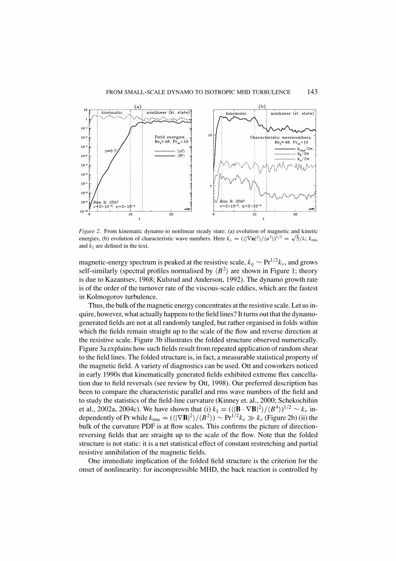
Figure 2. From kinematic dynamo to nonlinear steady state: (a) evolution of magnetic and kineticenergies, (b) evolution of characteristic wave numbers. Here kλ = (〈|∇u|2〉/〈u2〉)1/2 = √

5/λ; krms

and k‖ are defined in the text.

magnetic-energy spectrum is peaked at the resistive scale, kη ∼ Pr1/2kν , and growsself-similarly (spectral profiles normalised by 〈B2〉 are shown in Figure 1; theoryis due to Kazantsev, 1968; Kulsrud and Anderson, 1992). The dynamo growth rateis of the order of the turnover rate of the viscous-scale eddies, which are the fastestin Kolmogorov turbulence.

Thus, the bulk of the magnetic energy concentrates at the resistive scale. Let us in-quire, however, what actually happens to the field lines? It turns out that the dynamo-generated fields are not at all randomly tangled, but rather organised in folds withinwhich the fields remain straight up to the scale of the flow and reverse direction atthe resistive scale. Figure 3b illustrates the folded structure observed numerically.Figure 3a explains how such fields result from repeated application of random shearto the field lines. The folded structure is, in fact, a measurable statistical property ofthe magnetic field. A variety of diagnostics can be used. Ott and coworkers noticedin early 1990s that kinematically generated fields exhibited extreme flux cancella-tion due to field reversals (see review by Ott, 1998). Our preferred description hasbeen to compare the characteristic parallel and rms wave numbers of the field andto study the statistics of the field-line curvature (Kinney et. al., 2000; Schekochihinet al., 2002a, 2004c). We have shown that (i) k‖ = (〈|B · ∇B|2〉/〈B4〉)1/2 ∼ kν in-dependently of Pr while krms = (〈|∇B|2〉/〈B2〉) ∼ Pr1/2kν � kν (Figure 2b) (ii) thebulk of the curvature PDF is at flow scales. This confirms the picture of direction-reversing fields that are straight up to the scale of the flow. Note that the foldedstructure is not static: it is a net statistical effect of constant restretching and partialresistive annihilation of the magnetic fields.

One immediate implication of the folded field structure is the criterion for theonset of nonlinearity: for incompressible MHD, the back reaction is controlled by

144 A.A. SCHEKOCHIHIN ET AL.

Figure 3. The folded fields. (a) Sketch of the stretch-and-fold mechanism. (b) Cross-section of fieldstrength in a simulation of nonlinear dynamo (Pr = 500).

the Lorentz tension force B ·∇B ∼ k‖ B2, which must be comparable to other termsin the momentum equation. This quantity depends on the parallel gradient of thefield and does not know about direction reversals. Balancing B · ∇B ∼ u · ∇u, wefind that back reaction is important when magnetic energy becomes comparable tothe energy of the viscous-scale eddies. Clearly, some form of nonlinear suppressionof the stretching motions at the viscous scale must then occur. However, the eddies atlarger scales are still more energetic than the magnetic field and continue to stretchit at their (slower) turnover rate. When the field energy reaches the energy of theseeddies, they are also suppressed and it is the turn of yet larger and slower eddies toexercise dominant stretching. A model constructed along these lines (Schekochihinet al., 2002b) leads us to expect a self-similar nonlinear-growth stage during whichthe magnetic energy grows ∝ t and the rms wavenumber of the magnetic field drops∝ t−1/2 due to selective decay of the modes at the large-k end of the magnetic-energyspectrum. The folded structure is preserved with folds elongating to the size �s ofthe dominant stretching eddy. If Pr � √

Re, the culmination of this process isa situation where total magnetic and kinetic energies are equal, 〈B2〉 ∼ 〈u2〉,the fields are still folded with k‖ ∼ inverse box size, and krms has dropped bya factor of Re1/4 compared to the kinematic case. Since Pr � √

Re, we havekrms ∼ kνPr1/2Re−1/4 � kν still below the viscous scale. Thus the condition Pr �√

Re is necessary for krms and kν to be distinguishable in the nonlinear regime.It is possible that a second period of selective decay ensues, but this cannot bechecked numerically because the case Pr � √

Re � 1 is unresolvable and likelyto remain so for a long time. While astrophysical large-Pr plasmas are certainlyin this regime, the numerics can only handle

√Re > Pr �1 (or Pr � √

Re ∼ 1,see Schekochihin et al. (2004c) and Figure 3b). What can we learn from suchnumerical experiments? Our model predicts that the nonlinear-growth stage in sucha situation is curtailed with 〈B2〉/〈u2〉 ∼ Pr/

√Re < 1 and magnetic energy residing

FROM SMALL-SCALE DYNAMO TO ISOTROPIC MHD TURBULENCE 145

around the viscous scale. Note that all these estimates are asymptotic ones, sofactors of order unity can obscure comparison with simulations, in which onlyvery moderate scale separations can be afforded. With this caveat, we claim thatthe numerically observed state where there is excess magnetic energy at smallscales but overall 〈u2〉 > 〈B2〉 (Figure 1), is consistent with our prediction. Theratio 〈B2〉/〈u2〉 does increase with Pr, but a conclusive parameter scan is not yetpossible. Furthermore, the reduction of krms in the nonlinear regime, as well asthe elongation of the folds (decrease of k‖), are clearly confirmed by the numerics(Figure 2b).

Our model was based on the assumption of some effective nonlinear suppressionof stretching motions. This does not have to mean complete suppression of all tur-bulence in the inertial range. Two kinds of motions that do not amplify the field can,in principle, survive. First, the velocity gradients could become locally 2D and per-pendicular to the field (a quantitative model based on such two-dimentionalisationis described in Schekochichin et al., 2004b,c). One should expect a large amountof 2D mixing of the direction-reversing field lines leading to very fast diffusion ofthe field. If this happens, any selective decay must be ruled out, i.e., the nonlinear-growth stage cannot occur and 〈B2〉 cannot grow above the viscous-eddy energy.Since numerics support selective decay and saturated values of 〈B2〉 are certainly farabove the energy of the viscous eddies, we tentatively conclude that mixing due tothe surviving 2D motions is not very efficient. The second kind of allowed motionsare Alfven waves that propagate along the folded direction-reversing fields (Figure4). Their dispersion relation is ωk = ±(bb : kk)1/2〈B2〉1/2

, where b = B/B andk varies between the inverse length of the folds (∼box size) and kν (Schekochihinet al., 2002b). These waves do not stretch the field, do not know about the direc-tion reversals, and have the same properties as standard Alfven waves. However,Fourier transforming a field structure sketched in Figure 4 would not give Bk = uk

(scale-by-scale equipartition). Instead, the magnetic-energy spectrum would beheavily shifted towards small scales due to the presence of direction reversals. TheAlfven-wave component, while mixed up with folds in the magnetic field, shouldbe manifest in the velocity field. We therefore expect the kinetic energy to havean essentially Alfvenic spectrum, probably k−5/3. This picture accounts for theexcess small-scale magnetic energy observed in numerical simulations. Thus, weconjecture that the fully developed isotropic MHD turbulence is a superpositionof Alfven waves and folded fields. The advent of truly high-resolution numerical

Figure 4. Alfven waves superimposed on folded fields.

146 A.A. SCHEKOCHIHIN ET AL.

simulations should make it possible to confirm or vitiate this hypothesis in thenear future. A more extended exposition of the ideas presented above, as well asa detailed account of the numerical evidence, are given in an upcoming paper bySchekochichin et al., 2004c.

Acknowledgements

We would like to thank E. Blackman, S. Boldyrev, A. Brandenburg, andN.E. Haugen for stimulating discussions. This work was supported by the PPARCGrant No. PPA/G/S/2002/00075. Simulations were done at UKAFF (Leicester) andNCSA (Illinois).

References

Batchelor, G.K.: 1950, Proc. R. Soc. London, Ser. A 201, 405.Goldreich, P. and Sridhar, S.: 1995, ApJ 438, 763.Haugen, N.E.L., Brandenburg, A. and Dobler, W.: 2003, ApJ 597, 141.Iroshnikov, P.S.: 1964, Sov. Astron. 7, 566.Kazantsev, A.P.: 1968, Sov. Phys. JETP 26, 1031.Kinney, R.M., Chandran, B., Cowley, S. and McWilliams, J.: 2000, ApJ 545, 907.Kraichnan, R.H.: 1965, Phys. Fluids 8, 1385.Kulsrud, R.M. and Anderson, S.W.: 1992, ApJ 396, 606.Ott, E.: 1998, Phys. Plasmas 5, 1636.Schekochihin, A., Cowley, S., Maron, J. and Malyshkin, L.: 2002a, Phys. Rev. E 65, 016305.Schekochihin, A.A., Cowley, S.C., Hammett, G.W., Maron, J.L. and McWilliams, J.C.: 2002b, New

J. Phys. 4, 84.Schekochichin, A.A., Cowley, S.C., Maron, J.L. and McWilliams, J.C.: 2004a, Phys. Rev. Lett. 92,

054502.Schekochichin, A.A., Cowley, S.C., Taylor, S.F., Hammet, G.W., Maron, J.L. and McWilliams, J.C.:

2004b, Phys. Rev. Lett. 92, 084504.Schekochihin, A.A., Cowley, S.C., Taylor, S.F., Maron, J.L. and McWilliams, J.C.: 2004b, ApJ, in

press (preprint astro-ph/0312046).