MMK

TRITA-MMK 2002:2 ISSN 1400-1179

ISRN KTH/MMK/R—02/2--SE

Frequency Response of Hydraulic Hoses

JAN HÖLCKE

Stockholm

2002

Licentiate Thesis Department of Machine Design

Royal Institute of Technology, KTH 100 44 STOCKHOLM

TRITA-MMK 2002:2 ISSN 1400-1179

ISRN KTH/MMK/R—02/2--SE

Frequency Response of Hydraulic Hoses

JAN HÖLCKE

Licentiate Thesis Department of Machine Design

Royal Institute of Technology, KTH 100 44 STOCKHOLM

Frequency Response of Hydraulic Hoses Licentiate Thesis TRITA-MMK 2002:2 ISSN 1400-1179 ISRN KTH/MMK/R—02/2--SE �Jan Hölcke Department of Machine Design Royal Institute of Technology, KTH SE-100 44 STOCKHOLM

Summary Hoses can be components of fluid power control systems. To determine the dynamic behaviour of such systems you need to know the dynamic properties of the components included. This investigation aims to develop a method to determine these properties of hoses.

Nitrile-black-carbon is used in hydraulic hoses. A literature study gives that rubber is a very complex material. It is viscoelastic with a lot of non-linearities so it is not self-evident how to model the hose. Four different models are studied. One of them gives an idea of the static relation between the rubber tube and the reinforcing. Two of them take the dynamic properties of rubber into account. The fourth model is a second order black box model.

Laboratory tests have been done. The relationship between pressure changes and volume changes in hydraulic hoses at different frequencies is measured. Two seated valves were used, one for increasing and one for decreasing the pressure in the hose. The volume of oil coming out from the hose was measured with a cylinder.

Three different hoses are tested. The test results agree rather well with one of the dynamic rubber models and with the black box model, useful for control system analysis.

Preface Long time ago I deled with hydraulic control systems including hoses. The lack of dynamic data was a drawback and a method to determine these was not found. In the late eighties Mikael Theorin developed a method to digitally control seat valves. Then I saw a possibility to use this method to analyse hydraulic hoses and this work started. For all help and good advisements I got from Mikael, when I built my test equipment, I want to thank him. The main work was done in the early nineties.

The main part of the work was presented in Swedish in 1995. Since then very little has been done until Sören Andersson persuaded me to carry out this report. I want to thank him for this and all the advices concerning the performance of the thesis. Finally I want to thank Peter Collopy for his help with the English.

3

4

Contents 1 Introduction ............................................................................................................. 9

1.1 The aim of this investigation ............................................................................. 9 1.2 The scope of the investigation......................................................................... 10 1.3 Comments to the literature found.................................................................... 10

2 The construction of hydraulic hoses........................................................................ 11 2.1 Reinforcing...................................................................................................... 11 2.2 Materials used in the inner and outer tubes ..................................................... 12 2.3 Neutral angle ................................................................................................... 13

3 Properties of rubber................................................................................................ 15 3.1 Basic properties of rubber ............................................................................... 15 3.2 Linear viscoelastic behaviour .......................................................................... 17 3.3 Temperature and frequency-dependence of the mechanical properties........... 18 3.4 Shifting ............................................................................................................ 19 3.5 Measured properties in rubber hydraulic hoses ............................................... 20 3.6 Mathematical description of the elasticity modulus of rubber ....................... 21 3.7 The non-linear behaviour of rubber................................................................. 22

4 Theory.................................................................................................................... 27 4.1 The importance of the inner tube—a simplified static analysis ..................... 28 4.2 A first dynamic model .................................................................................... 32 4.3 A second dynamic model ............................................................................... 38

5 Measurements........................................................................................................ 43 5.1 Forced volume changes .................................................................................. 43 5.2 Forced pressure changes................................................................................. 44 5.3 “Problems” with valve control ....................................................................... 44 5.4 PCP controlled valves .................................................................................... 46 5.5 Experimental set-up........................................................................................ 47 5.6 The measuring computer ................................................................................ 48 5.7 Measuring method.......................................................................................... 49

6 Evaluation.............................................................................................................. 51 6.1 Compensation for oil compressibility ............................................................ 51 6.2 Handling the measurements ........................................................................... 51 6.3 Influence of the shape of the curve................................................................. 54 6.4 Evaluations in the second dynamic model ..................................................... 58

7 Results and discussion........................................................................................... 63 7.1 The second dynamic model ............................................................................ 64 7.2 Simple model – transmission function ........................................................... 68 7.3 Experience and views ..................................................................................... 73

References .................................................................................................................. 75 Appendix 1................................................................................................................. 77 Appendix 2................................................................................................................. 79 Appendix 3................................................................................................................. 81 Appendix 4................................................................................................................. 85 Appendix 5................................................................................................................. 87

5

6

Nomenclature

7

Symbol Definition Units a cross area of thread m2 A area of rubber specimen m2 A, A0, A1… coefficients AR cross area of model rubber rod m2 b thickness of rubber specimen m B, B0, B1… coefficients d diameter m DA average diameter of reinforcing m di inner diameter m E modulus of elasticity Pa E* complex modulus of elasticity Pa E’ elastic part of modulus of elasticity Pa E” viscous part of modulus of elasticity Pa f frequency s-1 F force in model thread N F0 force amplitude N Fa axial force N FR force in model rubber rod N Ft tangential force N G shear modulus Pa G* complex shear modulus Pa G’ elastic part of shear modulus Pa G” viscous part of shear modulus Pa K bulk modulus Pa l length of model linkage m L lead of winding m l� tangential length of model linkage m lh length of hose m lR length of model rubber rod m Nl number of reinforcing layers Nt number of treads per layer p pressure Pa ph highest pressure during pulse Pa pl lowest pressure during pulse Pa r radius m ri inner radius m rm interface radius m ry outer radius m s Laplace operator s-1 t time s T temperature K To reference temperature K

Ts characteristic temperature K Uarm volume constant of reinforcing strain m3 Ue elastic volume constant m3 Ue viscoelastic volume constant m3 UM volume constant of steel cording

movements m3

ur radial displacement m Ush shear volume constant m3 Ust strain volume constant m3 VO oil volume m3 VR inner tube rubber volume m3 x excitation position m X substitution Y substitution � hose constant Pa-1 � angle of winding rad � F angle of force in winding rad � hose constant - � hose constant - � hose constant - � radial length of model linkage m � phase angle rad �� original radial length of model linkage m � linear strain - � shear strain rad angle of model linkage rad Poisson ratio - � density kg/m3 � 0 reference density kg/m3 � normal stress Pa � r normal stress, radial Pa � z normal stress, axial Pa � � normal stress, tangential Pa shear stress Pa � circular frequency rad/s

8

1 Introduction

1.1 The aim of this investigation Evolution in machine design is moving toward faster, increasingly automated and ergonomically better designed machines. Efforts have also been focusing on saving energy in order to make the machines more effective. These trends also apply to hydraulic-powered machines, which nowadays feature rapid reaction systems utilising hydraulic control circuits as well as electronic. Systems controlling the pump in order to avoid delivering more power than is necessary.

Load-sensing systems are used for instance in motorised excavation and logging machines. These applications feature feedback loops consisting of pipes and hoses that communicate the highest load pressures required at any given moment. This feedback pressure will then control pump displacement, so that the pump does not need to work to affect pressures higher than just above those required by the load. These types of systems feature rather complicated controlling mechanisms involving many moving components and a range of materials. These components include for example the hoses in the feedback lines. As the feedback line is of fundamental importance for the behaviour of the whole system, it is important to understand the dynamic responses of the hoses.

Hydraulic hoses consist mainly of rubber—a remarkable material with viscoelastic properties. Both the elasticity and the shear modulus of rubber are functions of temperature, frequency and the amount of tension. This is why rubber hoses are difficult to manage efficiently using control-system technology. Rubber is a complex material and the need to understand the dynamics of rubber hoses is fairly recent, which means that there is little literature in this field. In 1969, Swisher [11] wrote, “Little significant dynamic data is known about hydraulic hoses. No hose manufacturer that [Swisher] contacted could give any dynamic response data.”. And little has been published since then.

The three main objectives of this study are: 1. Develop a method for measuring the change in volume of hydraulic hoses

as a dynamic response to frequency of the pressure input. 2. Add to the body of scientific knowledge in this research area. 3. Gather experimental data describing the dynamic behaviour of rubber

hydraulic hoses.

9

1.2 The scope of the investigation This investigation consists of a literature study and experimental measurements. The experimental section investigates the pressure to volume relationship at different frequencies, and includes measurements of three different-sized rubber hydraulic hoses.

The literature study was undertaken at the KTH library and showed that very little has been done within this area. The literature study has consequently mainly focused on two topics, the construction of hydraulic hoses and the properties of rubber.

The experimental section of the study attempts to describe the relationship between pressure and volume changes in a hydraulic hose in response to the frequency of the pressure changes. Seat valves have been used in the measurements. These have been subject to pulse modulation using a method described in section 5.4, with the help of a specially built control computer.

1.3 Comments to the literature found Much is written about transients in pipes bur very little about the dynamics of hoses. Webb, Stuntz and Basrai [15] analyses hoses as elastic elements without any frequency dependence. They are focused on the emission of particles from pulsated hoses.

Swisher and Doebelin [12] uses linearization and the curve presented looks like the static relation between volume change and pressure. The same does Swisher in reference [11]. Curves for hoses of different sizes are given by Ovsyannikov, Golubev and Karalyus. [7]

A very good analysis of stress and strain in reinforced hoses is done by van der Horn and Kuipers [3].

How to construct in rubber is told in the Swedish book “Konstruera i gummi”[5].

An American standard for testing hoses for automotive hydraulic brakes [9] includes only static tests. It was valid 1978 but withdrawn 1988.

The main part of the other references gives knowledge of the properties of rubber. [1,2,5,6,8,14] .

A short version in Swedish of this report is given in [4].

10

2 The construction of hydraulic hoses Hydraulic hoses are constructed along the following principles.

� Inner tube—the role of the inner tube is to enclose the hydraulic fluid. Therefore the inner tube must be fluid-tight and resistant to degradation by hydraulic fluids.

� Reinforcing—the role of reinforcing is to bear up to pressures that are transmitted through the hose via the fluid, thereby making the hose dimensionally stable. Reinforcing can consist of one to several layers of, for example woven steel wire.

� Outer tube—the function of the outer tube is to protect the reinforcing from wear and tear. The outer tube must therefore resist and withstand physical and chemical agents such as oils, solvents, UV light, temperature variation and ozone.

2.1 Reinforcing The reinforcing used in hydraulic hoses normally consists of high-quality steel thread. Generally speaking, this can be incorporated into hoses in several different ways. In hydraulic hoses specifically, spirally-wound or braided reinforcing is used (see Figure 2.1).

a b

Figure 2.1 Different types of reinforcing used in hydraulic hoses, a spirally-wound

reinforcing, and b braided reinforcing.

Spirally-wound reinforcing is made by either winding a number of individual threads individually or together in strips spirally along the direction of the flow through the hose. Strips consist of rubber-coated weaving, in which the warp gives the weave its strength, and the weft holds it together. Spirally-wound hoses always contain equal numbers of alternating layers of left and right-wound weave.

11

Braided reinforcing consists of braided strips. Each strip consists of three or more parallel threads. Braids are applied in one or more successive layers interspersed by thin layers of rubber to fill the spaces between the layers and lock the threads.

There are of course other types of reinforcing used in hoses, for example knitted reinforcement, however those are not used in hydraulic hoses and so are not investigated here.

2.2 Materials used in the inner and outer tubes The material used in most hydraulic hoses is nitrile-black-carbon rubber (NBR). Besides rubber polymers, NBR consists of a filler called carbon black. Carbon black increases the material’s hardness and durability. NBR also contains a plasticiser—an ester softener or another synthetic oil—partly for increasing its workability and partly for increasing its resistance against the cold. The internal damping of the material is also influenced by the content of acrylic nitrile (ACN)—the higher the amount of ACN, the better the damping.

Figure 2.2 The diagram shows the influence of the ACN content on rubber [5]

12

The ACN content not only influences damping, but also the oil-swelling and low-temperature properties of the material. Using a low ACN content combined with a cold-resistant plasticiser, will allow a rubber to remain flexible in temperatures as low as -55�C, however the level of oil-swelling in this material will be considerable. Using a high ACN content without a cold-resistant plasticiser will mean that the rubber will begin to stiffen at -10�C, but will not swell at all in oil.

2.3 Neutral angle One of the aims in hose production is to incorporate the reinforcing in such a way that the dimensions of the hose will change as little as possible under pressure loading. This is achieved when the direction of the reinforcement is aligned with the resultant of the tangential and axial forces [3,4]. This direction is called the neutral direction and can be derived by the Equations 2.3.1 and 2.3.2.

The axial force can be expressed as:

pdFa ���2

4�

(2.3.1)

and the tangential force by:

2

pdLFt��

� (2.3.2)

where L is the lead, �d is the circumference of the reinforcement, and � is the angle of the winding in the reinforcing. The winding angle (�)is given by:

L

d����tan (2.3.4)

The direction of the resultant is given by a combination of Equations 2.3.1 and 2.3.2:

dL

pdLdp

FF

a

tF

��

242

tan 2 �

�

���� (2.3.5)

�

��tan

12tan F

13

In order for the reinforcement to lie in the same direction as the resultant, then �F = � must be satisfied, which implies that , and the neutral angle will be 54,7�. Differences between the winding and the neutral angles result in the changes seen in Table 2.1.

2tan2��

Angle change Changes seen in the hose Length Diameter Volume

Smaller Decreases Increases Increases Greater Increases Decreases Increases

Table 2.1 Changes in hoses caused by variations in the winding angle.

14

3 Properties of rubber

3.1 Basic properties of rubber Rubber is a remarkable material due to its unique combination of useful properties and its low price. Rubber is readily accessible, simple to process, chemically stable and withstands weather.[14]

Vulcanised rubber has three important properties that separate it from other materials:

1. its ability to greatly extend and swiftly contract strongly, 2. its capacity to absorb great amounts of energy without breaking down (for

example about 150 times greater than steel per unit mass), and 3. the high values exhibited in the relationship between compressibility and

elasticity moduli (often up to 100, compared with 3 in many other materials).

The dynamic properties of rubber are similar with both springs and dampers. A

stress versus strain graph for rubber normally shows a complex elasticity modulus. The reason for this is that the results of measurements depend on how fast the strain is applied, and how much damping contributes to the force. During very slow measurements, the results only include the elastic energy-storing component, but in very fast measurements, the results contain large viscous-dissipative as well as elasticity components.

Normal testing of the elasticity modulus provides the vector sum of the two contributing parts of the complex modulus of elasticity. The shear modulus is normally measured to determine the dynamic properties of rubber. As with the elasticity modulus, the shear modulus (G*) is complex, and consists of one energy-storing part (G ') and one dissipative part (G"). The equipment for measuring G* is generally built in accordance with the principles shown in Figure 3.1. Using a magnet and a coil, an exiting force, , can be created. The arising oscillation will obey Equation 3.1.1.

)sin( tFo ��

)sin(0 tFxmbxAG

bAxG

�

�

����

��

���

(3.1.1)

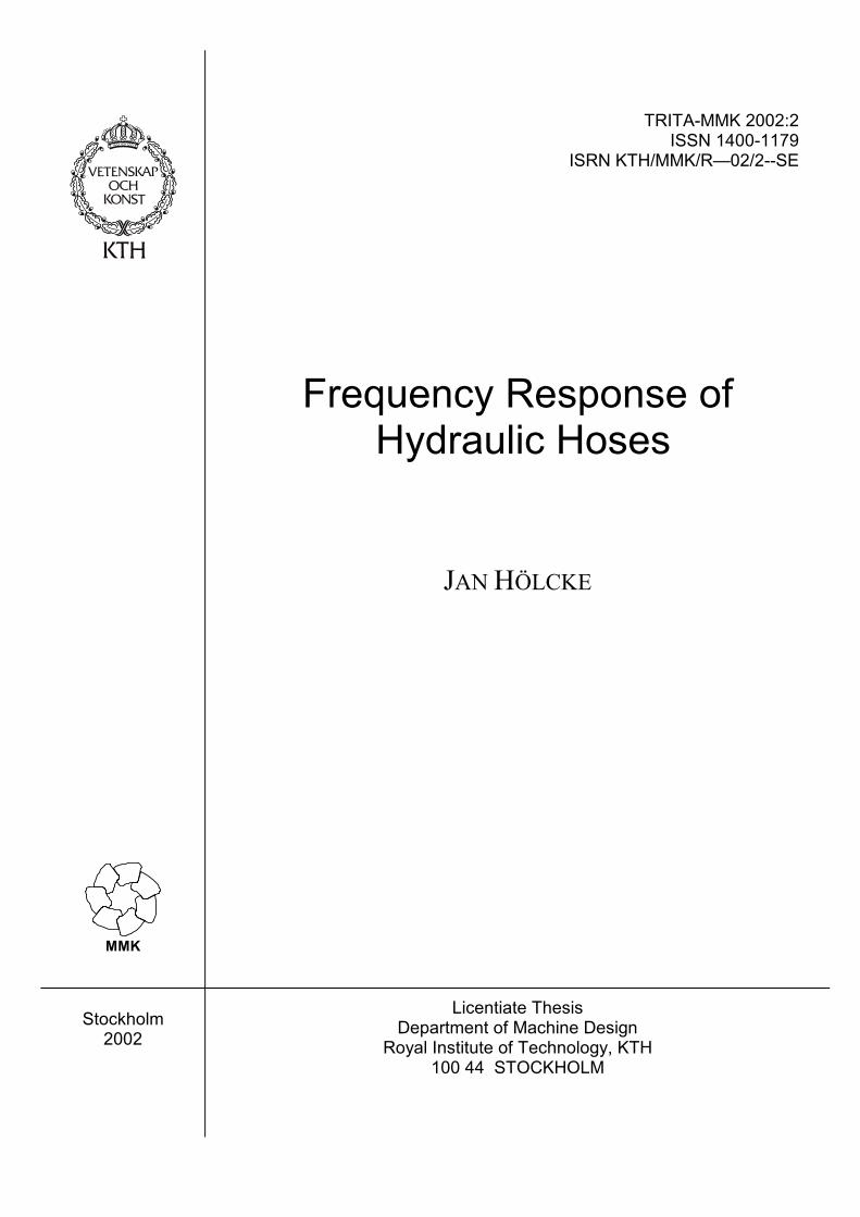
The area, A, and the thickness b of the rubber specimen as well as the position

x are shown in Figure 3.1 b.

15

a b

b

x�

A

Figure 3.1 The principle behind the equipment used for measuring the shear modulus of

rubber [14].

From the graph shown in Figure 3.2 below, showing ( 22 )()(* GG �����G ), it

is possible to calculate the shear modulus from the amplitude and the phase lag. In this way, a diagram such as the one shown in Figure 3.3 can be produced.

Time

Figure 3.2 Stress as a function of time, generated by sinusoidal movements [14]. Typical values for rubber at room temperature and at low frequencies can be seen in Table 3.1.

16

Table 3.1 Characteristic values of rubber at room temperature and low frequencies.[12] Modulus of elasticity E 0.6 – 60 MPa Shear modulus G 0.2 – 20 MPa Bulk modulus K > 700 MPa Poisson’s ratio � � 0.5

Figure 3.3 The complex shear modulus of rubber, including the components G' and G" [2,14]

3.2 Linear viscoelastic behaviour In a linear viscoelastic material, the relationship between stress and strain is a function of time (or frequency) and temperature. In rubber, the relationship between stress and strain is approximately linear at small amplitudes. It is possible to describe the relationship between tension and shear using Equation 3.2.1:

�� ����

�

���

��

�

��

���

�

���

��

�

� �� 2

2

2102

2

210t

Bt

BBt

At

AA (3.2.1)

where � is the strain angle[2] (see Figure 3.1b). When the input signal is sinusoidal, the formula can be written as follows:

� � � � ������ ������������� �� 22

1022

10 )()( BjBjBAjAjA (3.2.2)

or

17

� � ���� ������ )()( GjG (3.2.3)

where and G are the elastic and viscous components of the shear modulus. Denote the complex frequency-dependent shear modulus with G*(�). Then G and can be written:

G�

�

��

�

G�

� �)(*Re)( �� GG �� , G � �)(*Im)( �� G���

3.3 Temperature and frequency-dependence of the mechanical properties

The principle of superposition is applicable to linear materials. This implies that values of G* that are measured experimentally at one frequency and temperature, will equal values measured at another frequency and temperature. As temperatures decrease, so does the velocity of the thermal movements in the molecules. Because the deformation of rubber depends on these movements, the strain response to a change in stress will be slower, and the shear modulus (G*) will increase. If the temperature drops sufficiently low, the movements will almost cease entirely. The rubber will behave like glass (vitreous).

At higher temperatures, there is a plateau-like region, where the elastic part of the shear modulus (G ) and change only slightly. At very high temperatures, rubber starts to flow, becoming a highly-viscous fluid.

��

��tan

Between these three forms there are transfer zones. The five different states are: the vitreous region, the transition region, the rubber-elastic plateau, the rubber-flow region and the viscous region (see Figure 3.3). Note that the temperature is offset along the abscissa in a positive direction, and the frequency in negative direction. This shows that an increase in temperature in the rubber-elastic plateau causes the rubber to soften. At an increase in frequency, caused for example by a more rapid course of events, the rubber will instead be harder. This implies that an increase in temperature and a simultaneous increase in frequency will more or less match each other. If the complex shear modulus at the reference temperature T0 equals , at density , then it is possible to calculate the shear modulus at normal working temperature by:

*�rG 0�

�

�

�� TTGGr

00**�� (3.3.1)

The same formula is also valid for G and G [2]. � ��

18

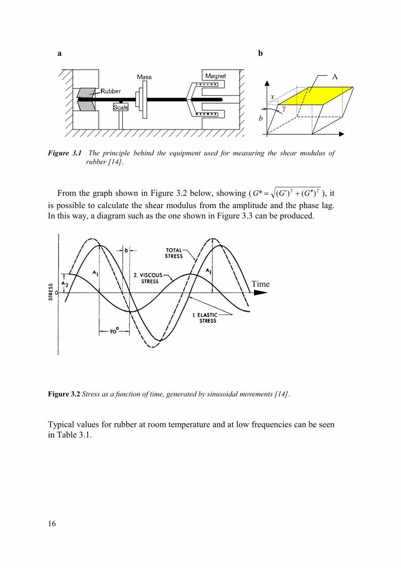
3.4 Shifting Most of the equipment for measuring shear or elasticity moduli in rubber work within a limited frequency region, but with a large variation in temperature. They also use shifting to increase the frequency domain of the curve. Shifting means that the short curves measured at different temperatures, represented by numbers 1 to 5 in Figure 3.4, are shifted horizontally, so that they fit the part of the curve measured at the reference temperature (T0,), in Curve 3.

1

2

34

5

log �

log G´( )�

Figure 3.4 An illustration of the principle behind shifting.[2,7]

In 1955 Williams, Landel and Ferry [16] found that the shifted graph follows a master curve expressed by the following equation:

s

s

T

T

TTTTs

��

��

�

6,101)(86,8

log�

�

(3.4.2)

In this expression Ts is a temperature characteristic for the material.

19

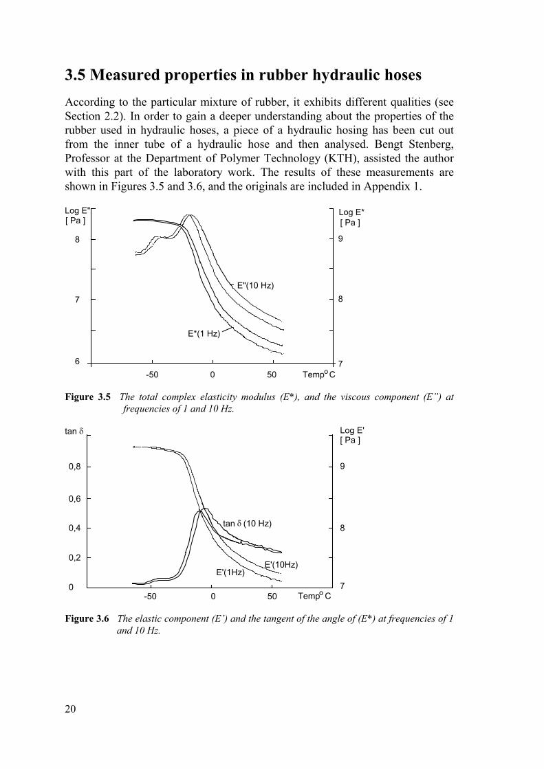
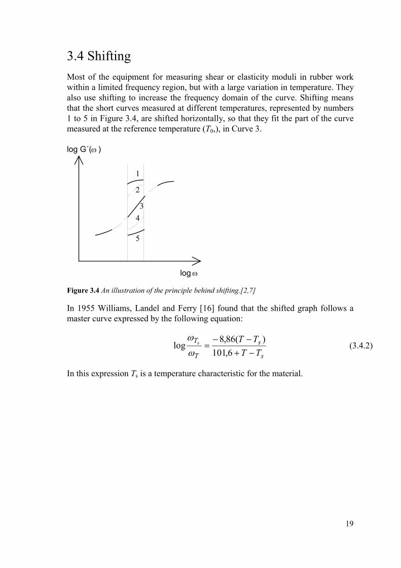
3.5 Measured properties in rubber hydraulic hoses According to the particular mixture of rubber, it exhibits different qualities (see Section 2.2). In order to gain a deeper understanding about the properties of the rubber used in hydraulic hoses, a piece of a hydraulic hosing has been cut out from the inner tube of a hydraulic hose and then analysed. Bengt Stenberg, Professor at the Department of Polymer Technology (KTH), assisted the author with this part of the laboratory work. The results of these measurements are shown in Figures 3.5 and 3.6, and the originals are included in Appendix 1. Log E"[ Pa ]

8

7

6-50 0 50 Temp Co

7

8

9

Log E*[ Pa ]

E"(10 Hz)

E*(1 Hz)

Figure 3.5 The total complex elasticity modulus (E*), and the viscous component (E”) at frequencies of 1 and 10 Hz.

tan �

0,8

0,6

0,4

0,2

0-50 0 50

9

8

7

Log E'[ Pa ]

E'(10Hz)

tan � (10 Hz)

E'(1Hz)

Temp Co

Figure 3.6 The elastic component (E’) and the tangent of the angle of (E*) at frequencies of 1 and 10 Hz.

20

3.6 Mathematical description of the elasticity modulus of rubber

In order to predict the properties of a system, one must be able to describe its components mathematically. Proceeding from the graphs in Figures 3.5 and 3.6 (and Appendix 1), the elasticity modulus at 30�C can be characterised by the following equations:

(3.6.1) 123,098,21 fE ���

(3.6.2) 160,029,6 fE ����

037,0286,0tan fEE

����

��� (3.6.3)

Figure 3.7 shows a plotting of these functions as well as those points on the curves in Figures 3.5 and 3.6 that form the basis for the calculations. The calculations are described below.

Figure 3.7 Plotting of the elasticity modulus of rubber in a hydraulic hose. E’ is marked using

diamond-shape points, E” by triangular-shaped points, and tan � with a dotted line.

The elasticity modulus of rubber is dependent on both temperature and frequency, with a change in frequency corresponding to a change in temperature. These changes must follow the master curve shown in Equation 3.4.1. According to Freakley and Payne [2], the characteristic temperature (TS) is about 45oK higher than the temperature at which the glass zone is entered. When TS is set to 30�C,

21

there will be good correspondence between the changes given by Equation 3.4.1, and the graphs in Figures 3.5 and 3.6. If commencing with a frequency of 1 Hz, and temperature settings of 30�C (TS and T), then temperatures will correspond to other frequencies according to Table 3.2.

Table 3.2 The relationship between temperature and frequency shifting according to the

master curve, (see Equation 3.4.1). Frequency [Hz] 0.001 0.01 0.1 1 10 100 1000 Temperature [�C] 82 60 43 30 20 11 4

By reading the values of log and from Figures 3.5 and 3.6, for the

temperatures listed in Table 3.2, and plotting them as functions of the logarithm of frequency, produces an almost linear function. The method of least squares gives the Equations 3.6.1 and 3.6.2. These calculations are shown in Appendix 2. Equation 3.6.3 is achieved by dividing Equation 3.6.2 by Equation 3.6.1.

E � E ��log

By adding a constant a model that fits the values even better is achieved, and with which the modulus of elasticity can be written as follows:

MPa (3.6.4) � � � �E f16 44 4 900 155, , ,

MPa (3.6.5) �� � � �E f5 06 1 020 1888, ,,

3.7 The non-linear behaviour of rubber Though rubber’s properties can often be described as approximately linear, it is also non-linear in different ways. For example, it has specific responses at small strains, and is influenced by previous loading events. It also exhibits a non-linear relationship between stress and strain during large changes, so the superposition principle is not applicable.

In vulcanised rubbers, non-linearity is caused by cross-bindings that burst at stress concentrations, due to the energy consumed at molecular extensions, and in some rubbers also due to stretching crystallisation. In the low-strain region, the non-linearities depend on the filler material—usually carbon black. The first time a piece of vulcanised natural rubber is stretched requires considerably more force than subsequent extensions, while at the same time these take on a curvilinear appearance as can be seen in Figure 3.8. The breakdown, which increases with increasing carbon black filler content, produces a uniform curve for various materials when the strain is standardised ( . Figure 3.9 shows tension as a function of normalised strain for a number of different sorts of rubber.

)/ max��

22

Figure 3.8 Changes in tension with repeated strains [2]. The softening up of the material depends on the breakdown of the filler material. If the rubber is allowed to rest a couple of days, then it recovers, and the material behaves once again as though it had not been previously treated. Tension [MPa]

Figure 3.9 Tension as a function of standardised strain ( for natural rubber

measured during the second strain cycle [2]. )/ max��

23

With very small strains, the rubber exhibits a very high shear modulus before the carbon black filler breaks down. The difference in rigidity between large and small shears is highly dependent on the amount of carbon black, because the high shear modulus depends on the shearing in the filler material (see Figure 3.10).

Töjningsamplitud topp till topp

Dynamiska skjuvmodulen G´ [ MPa ]� x

Strain amplitude top-to-top

Dynamic shear modulus G’�x [MPa]

Figure 3.10 The shear modulus of rubber with small strains and the influence of the carbon

black content [2]. In large strains ( ), Equation 3.7.1 applies, giving tension as a function of strain. Figure 3.11 shows the results graphically. The relationship does not appear to be linear in the normal working region, but hyperbolic.

16,0 ��� �

���

�

���

�

��� 2)1(

11�

�� G (3.7.1)

24

-3

-2,5

-2

-1,5

-1

-0,5

0

0,5

1

1,5

-0,6 -0,4 -0,2 0 0,2 0,4 0,6 0,8 1 1,2

Teoretisk relationekv (3.6.1)

Experimentelladata

Strain

Tension [MPa]

Theoretical relationship Equation 3.7.1 Experimental data

Figure 3.11 The tension-strain diagram for rubber at large strains[2].

25

26

4 Theory To cause a certain rise in pressure there needs a volume of oil to compress the oil already contained in the hose and a volume to expand the hose. The conditions surrounding the compression of oil are well documented and relatively easily handled theoretically, with enough precision for these sorts of applications, given that the oil is free from air bubbles. However the conditions surrounding the expansion of the hose are less well-investigated, as already pointed out in Chapter 1.

Hoses consist of three basic layers as previously mentioned: the inner tube, with the role of maintaining a fluid-tight seal; the reinforcing containing steel cording, with the role of bearing up to pressure forces; and the outer tube, with the role of protecting both the inner layers from wear and tear. With respect to resistance and strength, the hose can be characterised as having a soft inner tube with a rigid outer casing. The outer rubber casing is rather uninteresting from resistance point of view, and doesn’t influence the change in volume enough to make it worthwhile investigating. However even if the analyses are narrowed down to the two inner layers, then these still represent a very complex design with respect to resistance and strength. In broad terms, these two components are basically a soft rubber inner tube with a more rigid, reinforced steel sleeve. In the reinforcing layer, the interaction between the alternating steel cording and the layers of rubber constitute a difficult to analyse unit, where the rubber lying between the threads of cording can be considerably deformed (see Figure 4.1). As the distribution of the cording is often uneven, symmetry cannot be used to assist detailed analysis. a b

Figure 4.1 a A cross-section of a hydraulic hose. b A cut away view.

27

A simple model can be used to obtain an overall understanding of the inner tube’s role in the uptake of forces. In this model, the steel cording is replaced by a thin-walled steel tube.

4.1 The importance of the inner tube—a simplified static analysis

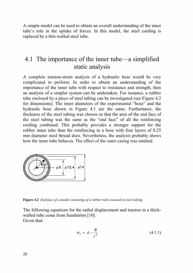
A complete tension-strain analysis of a hydraulic hose would be very complicated to perform. In order to obtain an understanding of the importance of the inner tube with respect to resistance and strength, then an analysis of a simpler system can be undertaken. For instance, a rubber tube enclosed by a piece of steel tubing can be investigated (see Figure 4.2 for dimensions). The inner diameters of the experimental “hose” and the hydraulic hose shown in Figure 4.1 are the same. Furthermore, the thickness of the steel tubing was chosen so that the area of the end face of the steel tubing was the same as the “end face” of all the reinforcing cording combined. This probably provides a stronger support for the rubber inner tube than the reinforcing in a hose with four layers of 0.25 mm diameter steel thread does. Nevertheless, the analysis probably shows how the inner tube behaves. The effect of the outer casing was omitted.

r �

z

Figure 4.2 End face of a model consisting of a rubber tube encased in steel tubing. The following equations for the radial displacement and tension in a thick-walled tube come from Sundström [10]. Given that:

2rBAr ��� (4.1.1)

28

2rBA���� (4.1.2)

and

constant�z� (4.1.3)

then

� � � � ��

���

����� r

rBrA

Eu zr ���� 111 (4.1.4)

and

� A�E zz ��� 21

�� (4.1.5)

In the above equations, A and B are constants that depend on the load on the inner and outer surfaces. Because a hydraulic hose is constructed to resist changing shape—in its diameter and length—then the steel cording effectively bears all the force. At the same time, the elasticity modulus of the steel is many times higher than the rubber’s, so that the small strains that arise in the steel do not affect the tension in the rubber to any great extent. Therefore it is assumed in this very simple model here, that there are no displacements in the axial direction ( ). This assumption does not influence the radial strain in the steel tubing to any great extent.

0�z�

When � , the following is obtained using Equation 4.1.5: 0�z

Az �� 2� (4.1.6)

When this is inserted into Equation 4.1.4, it gives the following:

� � � � ��

���

�����

rBrA

Eur ��� 1211 2 (4.1.7)

The same equations hold for both the rubber and the steel tubes. In the interface between the two, the tension and the displacement are equal. Furthermore, ( 0)( �yr r� ) holds true, because there is no pressure outside the steel tubing. Using the index S for the steel tubing and R for the rubber inner tube gives Equation 4.1.1.

20y

SS

rBA �� (4.1.8)

29

2i

RR

rBAp ��� (4.1.9)

In this equation, the tension in the inner edge is just as much as the oil pressure but with the opposite sign. Displacement at the interface between the steel and the rubber (of radius ) is just as large, therefore: mr

(4.1.10) � � � mrSmrR ruru � �

Through performing a number of calculations (see Appendix 3), the constants A and B can be determined for the steel and the inner tube respectively (see below).

2y

SS

rBA � (4.1.11)

� �

)()(

))(1(2222

2222

myimEE

imRyiS

rrYrrX

rrYrrpB

S

R������

������

�

�

(4.1.12)

where � � � �SySSm rrX ��� ����� 121 222 ,

and � � � �RiRRm rrY ��� ����� 121 222 .

� �

22

222

im

iymSR

rr

prrrAA

�

��

� (4.1.13)

(4.1.14) � pArB RiR ��2 �

By assuming that � , Pa, � , Pa (which is roughly true for low frequencies), � , and the pressure inside the “hose” is 10 MPa, and substituting these into the above equations, the following values are obtained for the A and B constants:

0�z910206 ��SE,0�R

3,0�S61020 ��RE

5

81009,1 ��SA Pa N 31034,5 ��SB

61097,9 ���RA Pa N 614,0�RB 30

With the help of these constants, the tensions and displacements can be shown graphically as in Figure 4.3.

-5,000E+01

0,000E+00

5,000E+01

1,000E+02

1,500E+02

2,000E+02

2,500E+02

0,0045 0,005 0,0055 0,006 0,0065 0,007

0

2

4

6

8

10

12Tension [MPa]

Radial displacement

Radial tension

Tangential tensionDisplacement [�m]

Radius r

Figure 4.3 Tensions and displacements in the wall of the tubing. The left hand side shows the

conditions in the rubber component. The descent in tangential tension occurs at the crossing over to the steel.

It can be seen in Figure 4.3 that the rubber behaves almost like a fluid. Both �r and �� are almost equal to the fluid pressure over the whole area. The divergence between the tension in the rubber and the fluid pressure, which can be studied closer in the underlying calculations for the diagram, show however that the rubber in the inner tube absorbs a small amount of the force, but that this is practically negligible. The conclusion that can be drawn from this is that almost all the compression force in the hydraulic hose is absorbed by the steel reinforcing—at least at low frequencies.

31

4.2 A first dynamic model As the pressure in a hydraulic hose is raised the hose changes volume. The amount of oil that has to be pressed into the hose in order to achieve a rise in pressure depends on several things: � compression of the oil in the hose, � compression of the rubber in the inner tube itself, � bulging of the rubber between the threads in the steel cording, � strain on the threads in the steel cording, and � movement in the steel cording. The total change in volume is obtained by adding together all the contributing factors mentioned above. Some of these are elastic by nature and are therefore not frequency-dependent, while others are viscoelastic in nature, and therefore strongly frequency-dependent. 4.2.1 COMPRESSION OF THE OIL The compression of the oil depends on the properties of the particular hydraulic fluid being used. Because changing the fluid can change the oil compression effects within the hose, it is therefore irrelevant to include the properties of the fluid in a description about the properties of the hose. The influence of the compression of the oil should therefore be subtracted from the measurements in the hose. During measurements, compression not only affects the oil in the hose but also the oil in the connecting lines and in the pressure sensors, the total oil volume (VO). The influence of the oil compression in these parts (�VO) must also be factored away (see Equation 4.2.1).

pV KV

OO��� (4.2.1)

32

4.2.2 COMPRESSION OF THE RUBBER

The literature contains very little in the way of information about the compressibility modulus for rubber. However it is claimed that at low frequencies this is normally greater than 700 MPa [ref]. It is unclear though how dependent it is on frequency. To avoid leaving it out of the general case, it is assumed that the rubber has a modulus of compression, bulk modulus, that is frequency-dependent—referred to as . When the volume of the rubber under compression (V ) is frequency-dependent, then the change in volume (�V

*RK

R R) in the inner tube can be expressed by:

pVR

R

KV

R ��� * (4.2.2)

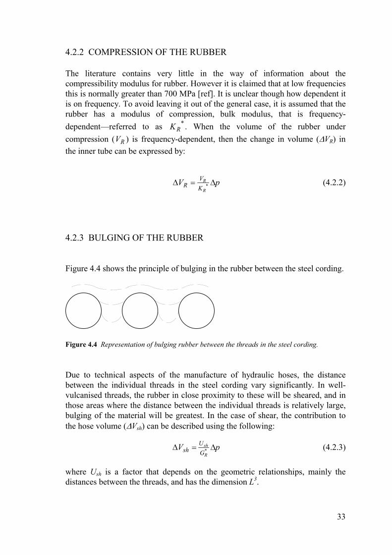
4.2.3 BULGING OF THE RUBBER Figure 4.4 shows the principle of bulging in the rubber between the steel cording.

Figure 4.4 Representation of bulging rubber between the threads in the steel cording. Due to technical aspects of the manufacture of hydraulic hoses, the distance between the individual threads in the steel cording vary significantly. In well-vulcanised threads, the rubber in close proximity to these will be sheared, and in those areas where the distance between the individual threads is relatively large, bulging of the material will be greatest. In the case of shear, the contribution to the hose volume (�Vsh) can be described using the following:

pVR

sh

GU

sh ��� * (4.2.3)

where Ush is a factor that depends on the geometric relationships, mainly the distances between the threads, and has the dimension L3.

33

For bulging where the strain is considerable, the following expression can be used instead:

pVR

st

EU

st ��� * (4.2.4)

In the same way as Ush in Equation 4.2.3, Ust in this expression is a factor that depends on the geometric relationships and also has the dimension L3. 4.2.4 MOVEMENT IN THE STEEL CORDING Figure 4.5 represents an example of shearing of the rubber between the steel cording layers when the hose is subject to pressure. a b

a b c

d

A Ba b c

d

A B

Figure 4.5 A representation of the shearing of the rubber between the cording layers; a un-

pressurised, and b pressurised. Where the threads in the reinforcing move relative to one another when the hose is subject to pressure (and therefore compressed), the layers of rubber in between the cording are subject to shearing. By way of example, take the steel cording located at a particular position along a hose shown in Figure 4.5. In the narrow space between threads a and b, the pressure is absorbed by the cording, and therefore the pressure in the rubber in area A is relatively low. In the area between threads b and c, lying further apart, the rubber moves more freely, and therefore the pressure is translated with only a slight reduction across into the area around B. Thread b is subject to a higher pressure on the lower right surface than on the lower left part. The resulting compression force then forces thread b to the left whereby shearing occurs in the rubber between b and d. This is accompanied by shearing forces that help to balance out the compression forces. The movement during pressurisation is also associated with an increase in volume. This increase in volume (�VM) is counteracted by shear forces in the rubber and can be expressed by:

34

pVR

M

GU

M ��� * (4.2.5)

where UM is a factor that depends on the geometry and has the dimension L3. 4.2.5 STRAINING THE REINFORCING The straining of the reinforcing is generally proportional to the pressure in the hose, and therefore also the change in volume. The latter can therefore be written:

pVS

armE

Uarm ��� (4.2.6)

where U is mainly described by the following: arm

����

����

sin83 3

aNNlLD

Ult

hAarm

� (4.2.7)

using the following parameter definitions. DA Average diameter of the reinforcing L Rise per reinforcing layer lh Entire length of the hose Nt Number of threads per layer Nl Number of reinforcing layers a cross area of thread

� Reinforcing angle 4.2.6 TOTAL VOLUME CHANGE The total volume change equals the sum of all the change components and can therefore be written:

(4.2.8) Oarmk

Mj

sti

shR VVVVVVV ������������� ���

where �VO gives the effect of the oil’s compression. The change in the volume can also be written as:

35

ppp

pppK

ldDV

KV

EU

kGU

jEU

iGU

G

hiA

O

S

arm

R

M

R

st

R

sh

������

��������

��

�

��

*

***

224 )(�

(4.2.9)

Given that all the changes in shape in the rubber—that are dependent on the molecules’ thermal movements—are affected equally by the thermal and dynamic changes (G ), then these terms can be divided up into elastic and viscoelastic terms:

**RR E�

pE

UE

UV eve ���

�

���

�� * (4.2.10)

where the viscoelastic term can be written:

pE

UEjE

UV eve ���

�

���

�

��

)()( ��

(4.2.11)

If this expression is to describe the hose characteristics properly, then when EE ��� och are known, Uve and Ue would be able to be ascertained from the

measurements of the hoses. The absolute value of the ratio between the change in volume and the change in pressure becomes:

2

22

2

22 ��

���

�

����

����

�

���

��

����

�

�

�

EEEU

EU

EEEU

pV veeve (4.2.12)

The curves shown in Figures 3.6 and 3.7 ought to be a good representation of EE ��� och for rubber other than the actual hoses tested here. By substituting

Equations 3.6.4 and 3.6.5 into Equation 4.2.12, curves of the shape seen in Figure 4.6 can be plotted.

36

|�V/�p|

1

1,0002

1,0004

1,0006

1,0008

1,001

1,0012

1,0014

1,0016

1E-06 0,00001 0,0001 0,001 0,01 0,1 1 10 100

Figure 4.6 Relative change in volume in a hose according to Equation 4.2.12, with rubber

characteristics according to Equations 3.6.4 and 3.6.5.

Figure 4.6 shows that as the frequency lowers the change in volume increases. This means that a hose should increase in volume the longer it is subjected to pressure, which contradicts all practical experience. Therefore another model has been developed, which is presented in the following section.

37

4.3 A second dynamic model When a hydraulic hose is subject to pressure, the shape of the steel cording changes in certain ways to adapt to the new equilibrium conditions. The tensile force in the steel threads is approximately proportional to the force applied. The steel threads are held in place by the numerous layers of rubber sandwiched between them. As noted earlier, the structure is complex and irregular. A model that can illustrate the exact conditions within a hydraulic hose is therefore very difficult to achieve, and would at the same time no longer apply to the general case as it would only apply to a specific hose.

When a hose is subject to pressure loading, large axial forces arise in the steel threads in the reinforcing cording. These are also subject to radial forces as well as shear forces from the surrounding rubber. In a non-pressurised state, every steel thread in the cording has one position, and when subject to pressure has another position. The rubber that lies in between the threads are therefore deformed. Consider a small piece of steel cording called �x in Figure 4.7a, and set the position of the adjoining steel cording to zero. When the hose is subject to pressure, the cording adopts a new position, shown by the dotted lines in the figure. A simple model of this can be developed by equating the cording in the unstrained position to two flexibly joined rods, linked together via a joint consisting of a “rubber spring” as in Figure 4.7b.

F F

Gummi

l

l

�

�

Fg

� FL

D

F F

Gummilg

a

b

c d

�x x Rubber

Rubber R

R

Figure 4.7 a Steel cording; b mechanical model of the steel cording; c cross-section along the

hosing; and d geometric conditions in one of the linkages from the mechanical model in b.

38

The following equation can be written based on the geometrical conditions shown in Figure 4.7d:

�

�lFF

R� (4.3.1)

The distribution of the compressive forces across the various steel threads in the cording, means that the force on an individual thread becomes the average force according to the following expression:

��

��

��

�tansin2sinsin

DN

DpN

pDLN

pAF � (4.3.2)

where N is the total number of threads, N = Nt�Nl. The strain in the “rubber rod” approximately follows the expression:

*0 EAl

F RR

R�� �

� (4.3.3)

At small angles, the peripheral length is expressed by:

)1()1(cos 2

22

22 lllll ��

� � ������ � (4.3.4)

When the strain on the cording is included, the peripheral length becomes:

)1)(1( 2

2

2 aEF

lll ���

�� (4.3.5)

where a is the cross area of the cording thread. With the original length

( )1( 2

20

20 lll �

� �� ) included in the equation, the change in length then becomes:

��

���

� ������� 2

20

2

2

220 11llaE

Fllll ���� O (4.3.6)

and the change in volume, surrounded by the cording, becomes:

VVlaE

F ���

���

� ���

2

220

23 �� (4.3.7)

Equations 4.3.1, 4.3.2 and 4.3.3 give the following expression for bulging (����

*tansin2

02

1 EAlNlDp

R

R�������

����

��

�� (4.3.8)

39

When this is inserted into Equation 4.3.7, the following expression is obtained for the change in volume:

VlaEN

DpV

ElANlDp

R

R

�

����

�

�

����

�

�

����

����

�

�

�� �

����

����

��

���2

*tansin2

2

20

2

21

112tansin2

3�

�� (4.3.9)

When the factors that depend on hose geometry are put together, the expression for the relative change in volume results in:

��

�

�

��

�

�

�����

����

�� 2)1(11

EjEpp

VV (4.3.10)

The above change in volume only takes into consideration the strain and the change in shape of the steel cording. The effects of factors such as the “hammocks” described in the previous section are not included. When the expression for the change in volume is complemented with terms for these effects, it them becomes:

EjE

ppVV

EjEp ����

�����

�

�

��

������ �

�

����

�� 2)1(11 (4.3.11)

Due to the properties of rubber, these functions are complex. The absolute amount can be expressed by:

� � � �� �

� �

4224

222

222

)(6)( where

)(2

)32()2()(

22

22

EpEEpEN

N

NpEpEEpE

pEEpEpEppN

VV EE

E

EEE

���������������

���������������������

�������������������������

� ����

��

����

�

(4.3.12)

This function is shown in diagrammatic form in Figure 4.8.

40

0

0,001

0,002

0,003

0,004

0,005

0,006

0,007

0,008

0,009

0,01

0,0 1,0 2,0 3,0 4,0 5

|�V/V|

Pressure [Mpa]

,0

�

Figure 4.8 The change in volume as a function of the change in pressure, using frequency as

the parameter. The circular frequencies sketched are 0,01 rad/s, 0,2 rad/s,5 rad/s and 50 rad/s. Used parameters: �=5�10-4Pa-1, �=2�10-3, �=10 and �=0,01

0

0,001

0,002

0,003

0,004

0,005

0,006

0,007

0,008

0,009

0,01

0,0 1,0 2,0 3,0 4,0 5,0

|�V/V|

Pressure [Mpa]

��

�

�

�

Figure 4.9 The effect of the constants (�, �, � and �) from Equation 4.3.11 on the shape of

the curve.

41

42

5 Measurements The objective of the study is to describe the relationship between pressure changes and volume changes in hydraulic hoses at different frequencies. Two different methods can be considered for measuring this. One is based on subjecting the enclosed volume in the hose to a forced volume change and recording the pressure changes that result. The other is based on subjecting the hose to pressure variations and to study the volume changes that result. Regardless of the method selected, small volume variations are being studied, which is why any sort of leakage would be devastating for the measurements.

5.1 Forced volume changes Forced volume changes can be achieved with the help of an eccentrically-driven piston. When using large hoses and low frequencies, a relatively large change in volume is required in order to obtain measurable pressure changes. However with small hoses and high frequencies, only small changes in volume are required so that the pressure increases don’t become too great. One or more absolutely leak-proof pistons are required for conducting these measurements over a wide range of frequencies.

43

5.2 Forced pressure changes Forced pressure changes can be achieved with the system shown in Figure 5.1. The cycle starts with the opening of Valve A, subjecting the hose to increased pressure. When half the cycle is complete, Valve A closes and Valve B opens. The amount of oil that runs out is then recorded by the volume recorder. When the whole cycle is complete, Valve B closes and Valve A reopens once again, commencing a new cycle.

�

� �

Figure 5.1 Circuit diagram showing the principle behind the forced pressure changes. The method of forced pressure changes have been used in this investigation.

5.3 “Problems” with valve control As previously mentioned, any sort of leakage disturbs the measurements. Consequently seated valves have been used, which are normally totally leak-proof in the closed position. In contrast, servo valves for example, exhibit way too much internal leakage to be used here. In addition, it is very important that both valves do not open at the same time at any point during the cycle. This may sound fairly simple to achieve, however has proven to be the contrary, especially with high frequencies.

At for example 50 Hz, the whole cycle should be completed in 20 ms. Each valve has therefore 10 ms in which to commence opening, culminate opening in the fully-open position, and then close fully again. Should both valves happen to be open at the same time, then the oil would flow from the source of the pressure directly to the measuring cylinder, and add a considerable amount of fluid to the volume, even when both of the valves are only open at the same time for a very short interval of time. In order for the correct volume to be measured, it is

44

necessary for one of the valves to be fully closed before the other one opens. In order to guaranty this, a short interval of time can be introduced as a safety margin, during which time both valves remain closed. However, in order to both pressurise and de-pressurise the hose in time, then the safety margin must be as short as possible. Valve speed, especially during closing, is heavily dependent on the viscosity in the oil around the anchor, and the supply pressure used. The setting of the safety margin must therefore satisfy opposing requirements. On the one hand, it has to be a long enough interval to be able to cover a range of valve-closing velocities, and on the other hand, it has to be as short as possible so it doesn’t interrupt the cycle. It is especially difficult in the frequency range 20-30 Hz to get the valves to pulse with stability independent of the pressure. This is clearly seen when the pressure is observed with an oscilloscope. If both valves happen to open at the same time, a plateau can be seen in the pressure curve, and the volume per pulse decreases markedly (see A in Figure 5.2). Therefore the lower limit of the measuring points ought to be studied in the evaluation.

0 50 [ms]t

0

50 bar

p

A

Figure 5.2 Pressure curves, where the continuous line shows a correct pressure cycle, and the

dashed line represents a pressure cycle wherein both the valves are open during a pressure dropping cycle. At point A, the curve tends to flatten out approaching half the supply pressure.

45

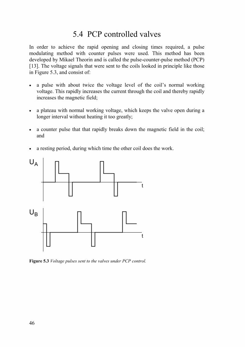
5.4 PCP controlled valves In order to achieve the rapid opening and closing times required, a pulse modulating method with counter pulses were used. This method has been developed by Mikael Theorin and is called the pulse-counter-pulse method (PCP) [13]. The voltage signals that were sent to the coils looked in principle like those in Figure 5.3, and consist of: � a pulse with about twice the voltage level of the coil’s normal working

voltage. This rapidly increases the current through the coil and thereby rapidly increases the magnetic field;

� a plateau with normal working voltage, which keeps the valve open during a

longer interval without heating it too greatly; � a counter pulse that that rapidly breaks down the magnetic field in the coil;

and � a resting period, during which time the other coil does the work.

t

t

U

U

A

B

Figure 5.3 Voltage pulses sent to the valves under PCP control.

46

5.5 Experimental set-up The hydraulic part of the experimental set-up used in the study is shown in Figure 5.4 below.

M

M V1

TG

V2

AV1

V3 V4

V5AV3

TBV

MC

AV2

Test object

Figure 5.4 Experimental set-up used in the study.

A relatively constant pressure was maintained using a hydraulic test bench. This was established and maintained using a calibrated manometer (M). The test object, the hose, is subject to pressure by opening the seated valve (V1). The pressure is registered by the pressure sensor (TG), connected via an amplifier to both the computer’s A/D transducer and an oscilloscope.

During the unloading phase, Valve 2 (V2) opens, whereby the oil stored in the test object flows further on to a measuring cylinder (MC). On the piston side of the cylinder, the oil is led through a pressure-limiting or backpressure valve (TBV), or through a cut-off valve (AV3), and further on via the seated valve (V4), open during measuring, and into the tank. The lower pressure in the pressure-loading cycle can be controlled using TBV and AV3.

De-airing the test object is done by opening the cut-off valve (AV1), and during the trimming of the pulses, the cut-off valve (AV2) is opened so that a return stroke with the measuring cylinder can be avoided. The measuring cylinder’s return stroke arises when valves V3 and V5 are open and the other three seated-valves are closed. The level in the measuring cylinder is registered by a sliding-potentiometer-type level indicator. This is also connected to one of the computer’s A/D transducers.

47

5.6 The measuring computer In order to control and collect the measurements, a special Z-80 based microcomputer was built (see Figure 5.5 for an overview). For communicating with the surrounding environment the computer features: � a driver (L 298) for the coils located on the measuring valves—by varying the

input to this driver, the high voltages can be achieved for the pulsations, and the low voltages for keeping the valves open (see Figure 5.3);

� outlets for controlling the valves that manoeuvre the measuring cylinder; � power supply to the pressure sensor and level indicator; � an input terminal with a differential amplifier for registering the pressure in the

hose; the amplifier is connected to an 8-bit A/D transducer (ADC 820).The amplification is set so that one unit in the A/D transducer is equivalent to 1 bar;

� input terminal for registering the level of the measuring cylinder connected to a 12-bit A/D transducer (AD 574);

� a keyboard; � an LCD display of 2 x 40 characters (DMC 40218); and � an RS 232 outlet (MAX 238), for transferring measurement results to a PC for

evaluation.

+- ADC820

AD579

CPU SIO

PIO

EPROM

RAM

CTC

TANGENT-BORDDISPLAY

L298

MÄTCYL-SPOLAR

PULS-SPOLAR

MAX238 PC

OSCILLO-SKOP

AD574Cylinder-läge

Tryck

RS232

i

Figure 5.5 The principles behind the Z-80 based measuring computer.

48

5.7 Measuring method Measurements have been performed on three different hoses with the following dimensions: Table 5.1 Test hose dimensions. Test hose Diameter

(inch) “Free” length

(mm) A 3/8 300 B 3/8 1031 C ¾ 275

The length of the visible part of the hose, that is that part of the hose that has

the ability to expand “freely” has been shown in Table 5.1. Elastic deflection in the walls, and the oil in those parts of the system between

the filling and draining valves in the test object must be calculated out. In order to determine the effect of the compression of the oil, so that it can be compensated out of the hose dynamics, the tests have been performed with various different lengths of hydraulic pipes, as well as totally without hose or steel tubing; that is with the pressure sensor mounted as close to the valves as possible.

The temperature in the hydraulic system has been maintained around 40oC to ensure the correct functioning of the seated valves. Because the oil that flows through the valves is not forced out of the hose, the tank temperature does not directly affect the temperature of the oil in the hose. Due to the internal friction in the rubber, a certain amount of energy develops with an associated rise in temperature within the walls of the hose. The ambient temperature was around 25oC.

In order for the temperature in the system to establish equilibrium prior to the commencement of measurements, the system is run at a pulse frequency of around 1 Hz for at least half an hour.

The supply pressure was varied manually between 20-80 bar, and a frequency series has been registered for each pressure.

A special low-pressure measurement has also been undertaken. During the preparatory investigations for these measurements, the pulsations from the pump were so worrisome that an accumulator was mounted on the supply line.

49

The programme in the measuring computer has been constructed so that it automatically loops through a number of pulse frequencies. At each frequency, the measurements have been made in the following way. 1. Pulsing commences. 2. Pulsing continues for one second so that the valve-hose system reaches a

stable operating condition. 3. The piston can move at least 0.5 mm to avoid the occurrence of transients in

the cylinder. 4. The number of pulses required for the cylinder to move a certain distance are

counted, and the number recorded. 5. When the measuring cylinder has moved the required distance the pressure

cycle is measured and recorded during one pressurising cycle. 6. The cylinder returns to its original position, the frequency is changed and the

measuring cycle commences again from Point 1 above, until all the measuring frequencies have been completed.

Once all the frequencies have been completed, or after a termination, the results of the measurements are transferred to a PC.

Due to the PCP control’s strong transients, spikes occur in the pressure measurement signal. Filtering out these digitally without losing the actual pressure-change data proved difficult. Attempts to determine the pressure differences for the various frequencies has been done using both the method of least squares and Fourier analysis, in order to determine the pressure differences for the various frequencies. Due to the above-mentioned disturbances, and the pulse shape changes at different frequencies, the automatic evaluation of the pressure differences became uncertain. Reading the pressure differences on an oscilloscope and manual input gave a reliable value.

The equipment has also provided the possibility of varying the discharging pressure. Varying the discharge pressure has not produced any noticeable influences on the measurements.

50

6 Evaluation

6.1 Compensation for oil compressibility In a study of a system containing a hydraulic hose, it is conceivable different kinds of fluids could be used. These can have different compressibility moduli. The influence from the hose should also therefore be separated from the influence of the hydraulic fluid. Compression of the oil in the hoses has therefore been subtracted from the measured results in this investigation. In order to shed light on how large this effect might be, a series of tests has been conducted using pipes of different lengths and diameters instead of hydraulic hoses. The change in volume as a function of the volume of oil in the pipe has been found to obey the following expression:

OVpV

����

� 0681,078,2 (6.1.1)

where VO is the oil volume. The development of this expression can be found in Appendix 5.

6.2 Handling the measurements In the simple dynamic model discussed in Section 4.2, the change in volume is assumed to be proportional to the pressure. Assuming this to be true, the following evaluation method has been used.

Specific supply and outlet pressures have been preset for recording each measurement series. This has been done in the manner described in Section 5.5. During the long pulses, the pressure in the hoses has managed to attain measurement and return pressures. During the shortest pulses, at the highest frequencies, the valve capacity has not been sufficient to fully raise and drop the pressures. Therefore at high frequencies, the pressure differences that the hoses are subjected to are reduced.

A good principle for studying the influence of various effects, is to keep all the parameters constant except for one, and then to study the influence of that variation on the signal. Then take each of the other parameters one at a time, and study their influences in the same way, until all of them have been studied. Because the pressure changes in this case are influenced by the pulse frequency, this method is not possible. Therefore for each and every one of the frequencies, the volume changes have been plotted as a function of the change in pressure.

51

From this diagram, the ratio of the change in volume and the change in pressure has then been determined. The ratios that have been determined for each frequency have then been compiled as a function of the pulse frequency. In practical terms, the assessment work has proceeded in the following way.

During measurement, the measuring computer has registered the pulse interval and the number of pulses required for moving the measuring cylinder a certain measurable distance. These data have then been transferred to a PC, which already contains the manually recorded pressure differences. The programme that receives the information, then stores the hose data in a file along with the pulsing frequency, pressure differences, and the volume differences per pulse compensated for the oil’s compression effects. Because the hoses have been pulsed at a number of different pressures, 5-10 such files have been created for each hose.

With the help of another programme, these files have been read, the data re-stored and written to new files—one file for each frequency. These new files contain the volume changes as a function of the pressure change, and the output has been adjusted for using directly in a curve-plotting program.

Any possible “lethargy” in either the filling or the draining valves, or both, will lead to their both being open at the same point in time. If this occurs, even for a fraction of a pulse interval, then this will affect the measurement results in such a way that the hose will appear to have a considerably larger expansion in volume than it actually does in reality. This has happened at Point P in Figure 6.1.

Figure 6.1 Measurement results from Test hose A at a frequency of 45,9 Hz.

52

The ratio of �V/�p ought to be determined by the slope of the line that lies at the lower margin of the set of points. It is however doubtful whether it is correct to simply blindly apply this method. If the diagram in for example Figure 6.2 is studied, there are three points in line with one another, and a fourth point (P) below these. The question can be raised, whether or not another type of measurement error that has crept in here.

A tendency to differ can be seen between the chordal and tangential values for in Figure 6.2. Using classic automatic-engineering analysis, non-linear

functions are linearised around a working point. What is interesting for these analyses here, is the tangential value for pressures over 35 bar. This is because the pressure level at the working point normally lies somewhere around half the supplied pressure level, which is usually at least 70 bar. In the next chapter, the tangential values that are presented in the diagram are discussed.

pV �� /

Figure 6.2 Measurement results for the Test hose B, at a frequency of 4,16 Hz.

53

6.3 Influence of the shape of the curve If the change in volume is seen as a result of an application of pressure, then the pressure-application cycle should affect the change in volume. At low frequencies, the pressure-application cycle is basically a square wave. At high frequencies, the pressure-application cycle approaches a triangular wave. In order to gain a better understanding of these effects, the changes in triangular and square waves have been studied as they pass through a low-pass filter (see Figure 6.3).

11+j��

Figure 6.3 Square waves passing through a low-pass filter. The input signal must undergo Fourier development in this analysis. This is

done by writing the input signal as a sum of sine and cosine terms, as in the set of equations below.

)sincos(2

)(1

0��

�

���

nnn tnbtnaatf �� (6.3.1)

where �,2,1,0cos)(2��� �

�

ndttntfT

aTc

cn �

and �,3,2,1sin)(2��� �

�

ndttntfT

bTc

cn �

f(t)

tT/2-T/2

1When the signal is a square wave like the figure to the right, then by substituting the following,

� ��

��

2/

0

sin14

,2,1,00T

n

n

dttT

b

na

�

�

the square wave can be written as:

���

�

��

���

1

2)12(

4 )12(sin)(n

Tn tntf �

�

� (6.3.2)

54

When passing through the low-pass filter, the amplitude is reduced in the following way:

� �2

00 1

11

1

�

��

�

�

�

� j (6.3.3)

and the oscillation with the various frequencies is phase shifted in the following way:

0

arctan1

1arg0

�

�

�

�

�

� j (6.3.4)

The function for the output signal can be written as: (6.3.5)

� �� ��

�

�

�

��

�

��

��

����

�

��

1

2)12(222)12()12(

40

0

arctan)12(sin1

1

nTn

T

Tnn tny

�

��

�

�

�

-1,5

-1

-0,5

0

0,5

1

1,5

-50 0 50 100 150

-1,5

-1

-0,5

0

0,5

1

1,5

0 0,05 0,1 0,15

a b

-1,5

-1

-0,5

0

0,5

1

1,5

-0,02 0 0,02 0,04

-1,5

-1

-0,5

0

0,5

1

1,5

-0,005 0 0,005 0,01 0,015

c d

Figure 6.4 Changes in a square wave during passage through a low-pass filter with a switching frequency of 12,7 Hz; a where the input signal’s frequency is low <0,1 Hz; b f = 10 Hz; c f = 30 Hz; d f = 100 Hz.

55

f(t)

t-T/2

1

-T/4 T/4 2T/4 3T/4

For the triangular wave, the corresponding substitutions apply:

��

���

���

� ��

4

4

43

4

sin)2(sin

,2,1,00

442T

T

T

T dttndttnb

na

Tt

Tt

Tn

n

��

�

The terms for are calculated, after which the triangular wave can then be written as:

nb

���

�

��

��

���

�

1

2)12()1(8 )12(sin)( 22

)1(

nTn

tntfn

�

�

� (6.3.6)

The function for the outgoing wave after it has passed through the low-pass filter can be written as follows:

� �

���

�

�

��

�

����

��

����

�

��

�

1

2)12(222)12()12(

)1(80

0

22

)1(arctan)12(sin

1

1

nTn

T

Tnn

tnyn

�

��

�

��

� (6.3.7)

-1

-0,5

0

0,5

1

-5 0 5 10 15

-1

-0,5

0

0,5

1

-0,05 0 0,05 0,1 0,15

a b

-1

-0,5

0

0,5

1

-0,01 0,01 0,03

-1

-0,5

0

0,5

1

-0,005 0 0,005 0,01 0,015

c d Figure 6.5 Changes in a triangular wave during passage through a low-pass filter with a

switching frequency of 12.7 Hz; a where the input signal frequency is low <0.1 Hz; b f = 10 Hz; c f = 30 Hz; d f = 100 Hz.

56

0,1

1

0,01 0,1 1 10

Figure 6.6 The change in amplitude for triangular (�) and square (�) waves during passage

through a low-pass filter, as a function of the ratio of the pulse frequency and the filter’s switching frequency.

The changes in amplitude in the triangular and square waves are presented graphically in Figure 6.6. It can be seen in the graph, that the amplitude relationship between the input and output signals changes more at lower frequencies in triangular waves than in square waves.

The amplitude of the fundamental tone in the triangular wave is less than the top-to-top value for these waves. Because rigidity in the hose increases with increasing frequency, the overtones (harmonics) contribute less to the increase in volume than the fundamental tone. It can therefore be expected that a triangular wave causes a lesser change in volume than a square wave with the same top-to-top value. According to the theoretical analyses in Section 4.2, then the rubber’s damping effect will be less than the simple time constant that is assumed in the analysis above, and which resulted in Figure 6.6. Therefore an iterative method is required for the evaluation. The measurements provide input data for the adjustment of the theoretical functions according to Section 4.2. These provide information about the compensation of the measurements of the various wave shapes. The compensated measurement values provide new input data for the adjustments of the constants in the theoretical formulae and so forth.

57

6.4 Evaluations in the second dynamic model In the diagram produced for the evaluation described in Section 6.2, it can be seen that at high pressure differences, a tangent is obtained that does not pass through the origin, but crosses the ordinate further up. For hose B, this line crosses the y axis at approximately 100 mm3/pulse (see Figure 6.2). The constant � in Equation 4.3.11, should be such that �·V is also found to be approximately 100 mm3/pulse, compare Figure 4.9. It appears to be the case that the hose characteristics follow a function of the type described by the curves in Figure 4.8. It is also reasonably clear that the curve for the change in volume as a function of the pressure has a steeper initial part and a flatter latter part with higher pressure. This has also been shown by Ovsyannikov, Golubev, Karalyus [7] and Swisher and Doebelin [12].

During the pulsation measurements, the pressure at low frequencies swung between supply and atmospheric pressures, while at high frequencies, it fluctuated around a relatively low amplitude—about half the supply pressure. At low frequencies, the volume changes will therefore contain both the steeper part and part of the flatter section. At high frequencies on the other hand, the pressure differences during most of the measurements, lie only along the flatter part of the curve. This raises the question as to whether the decrease in the volume change, that was recorded at high frequencies, depended only on the fact that pressure was supplied in another way at those frequencies. How then should these measurements be used?

Assuming that there are a number of values containing slight recording errors, and a function that describes the cycle adequately has been measured. Given the assumption that the pressure changes that were able to be observed, only cover a fraction of the pressure range, then by linking them together, they can form a chain covering the whole range. If maximum and minimum pressures for the various measurements had been easily determinable, then a measurement series could have been produced in the same manner as Figure 6.7. By placing these measurements one after the other, a diagram agreeing with Figure 6.8 can be obtained.

58

tryck

voly

män

drin

g

0123456789

10

0 1 2 3 4 5

Pressure

Volume change

Figure 6.7 A conceivable measurement series showing the volume change for various pressure differences at various frequency levels.

Because the pressure obtained with rapid pulsing depends on the supply pressure, the pulse parameters, and the hose characteristics, the measuring set-up has not allowed a simple method for controlling these. Instead, the maximum and minimum pressures have been what they have been. The real measurements cannot therefore be stacked as elegantly as those shown in Figure 6.8, and a slightly more complicated method has to be applied.

tryck

voly

män

drin

g

0123456789

0 1 2 3 4 5

Pressure

Volume change

Figure 6.8 The measurement results according to Figure 6.7, assembled in a curve.

59

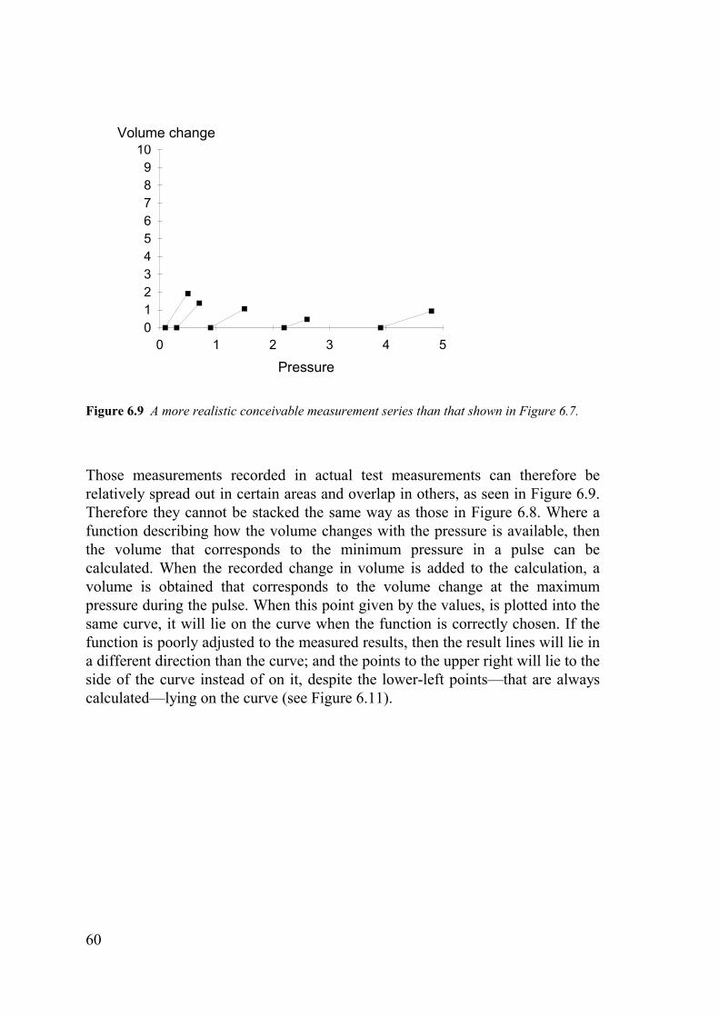
tryck

voly

män

drin

g

0123456789

10

0 1 2 3 4 5

Pressure

Volume change

Figure 6.9 A more realistic conceivable measurement series than that shown in Figure 6.7. Those measurements recorded in actual test measurements can therefore be relatively spread out in certain areas and overlap in others, as seen in Figure 6.9. Therefore they cannot be stacked the same way as those in Figure 6.8. Where a function describing how the volume changes with the pressure is available, then the volume that corresponds to the minimum pressure in a pulse can be calculated. When the recorded change in volume is added to the calculation, a volume is obtained that corresponds to the volume change at the maximum pressure during the pulse. When this point given by the values, is plotted into the same curve, it will lie on the curve when the function is correctly chosen. If the function is poorly adjusted to the measured results, then the result lines will lie in a different direction than the curve; and the points to the upper right will lie to the side of the curve instead of on it, despite the lower-left points—that are always calculated—lying on the curve (see Figure 6.11).

60

tryck

voly

män

drin

g

0123456789

10

0 1 2 3 4 5Pressure

Volume change

Figure 6.10 The measurement results (heavy black line) plotted together with the curve that

describes the cycle well. The points to the lower left are calculated and are therefore affixed to the curve.

tryck

voly

män

drin

g

0123456789

10

0 1 2 3 4 5

Pressure

Volume change

Figure 6.11 The measurement results (heavy black line) plotted together with the curve that describes the cycle poorly.

The measurement results have been treated in the manner described above. The constants �, �, � and � in Equation 4.3.12, have been adjusted using the method of least squares (see also Figure 4.9).

61

62

7 Results and discussion The objectives of the study included not only developing a measurement

method for, but also increasing our understanding of hydraulic hoses through describing their dynamic properties. The measurement method developed and used in the study, can be seen as having produced a good result, but with limitations regarding accuracy, frequency and capacity. Improvements to the test rig are discussed in Section 7.3, along with the experience gained from experimental hose pulsing, and further views about continuing the work.

With respect to describing the dynamic properties of hydraulic hoses, the results of the study can be summarised by two different equations, found in Sections 7.1 and 7.2. These mathematical expressions describe the properties of the hoses in different ways, and are applicable in different contexts. The second dynamic model, based on the theories presented in Section 4.3, can be found Section 7.1. This expression ought to be useful in connection with simulations. The simpler expression presented in Section 7.2, provides an estimation that does not apply to low pressure situations, but is nevertheless useful in connection with classic automatic-engineering analysis. Because these results are based on measurements of three specific hoses only, it ought to be pointed out that the formulae presented below should not be taken as general expressions for all hydraulic hoses.

63

7.1 The second dynamic model In Section 4.3, a second dynamic model for hoses was developed. This is

expressed as follows:

EjE

ppVV

EjEp ����

�����

�

�

��

������ �

�

����

�� 2)1(11 (7.1.1)

This expression contains four constants, �, �, � and � that are determined by

the experimental measurements. The method described in Section 6.4 (Evaluations in the second dynamic model) has been used. Out of all the measurements performed, only those recorded at frequencies of 0.2 and 5 Hz, and the highest frequency for the actual pressure supplied have been presented in this analysis. The frequency used at high pressure measurements was 45 Hz, but at low pressure, the highest frequency reached during the measurements was only around 35 Hz. These particular measurement values were chosen because the aim was to present an adequate spread of frequencies but without making the work too comprehensive to grasp. The values for Hose B have been plotted in Figure 7.1.

0

200

400

600

800

1000

1200

0 2 4 6 8

�V [mm3]

Pressure [MPa]

10

Figure 7.1 Measurements for Hose B, plotted in a diagram according to the method in Section 6.4, at frequencies of 0.2, 5 and 45 Hz.

64

By varying the constants in Equation 7.1.1, the curves have been adjusted to the recorded measurements. This has been done in part using a fully manual routine, and in part using the method of least squares with variable weighting. In this way, a “subjective” approach has been taken to handling measurement error, and the influence of triangular-shaped pressure application at high frequencies, as well as to possible warming effects. Good agreement is shown in Figure 7.2, where the constants have the following values: � = 5·10-4 Pa-1, � = 2·10-3, � = 3 and � = 0.01. It can be seen here that the main trends in the curve are correct, but that the high-frequency measurements lie below their corresponding curve. Considering that the pressure supplied had triangular-shaped waves at high frequencies, then this tendency can be seen to be correct.

At low pressure, the measurements lie in the reverse manner with respect to the curves. There can be many reasons for this; for example the movements in the rubber are relatively important here, and warming effects can therefore have a greater impact. It ought to be noted that the measurements plotted here using circles are measured at around 35 Hz for low pressure.

0

100

200

300

400

500

600

700

800

900

1000

0 2 4 6 8 10

Meas. 0,2 HzTheor. 0,2HzMeas. 5 HzTheor. 5 HzMeas. (35) 45 HzTheor. 45 Hz

Change in volume/Pulse

Pressure [MPa]

[mm3]

Figure 7.2 Measured values for Hose B together with theoretical curves according to

Equation 7.1.1. The values for the constants are: � = 5·10-4 Pa-1, � = 2·10-3, � = 3 and � = 0.01.

65

This was the highest frequency at which the valves worked adequately when the pressure was under 1 MPa. As already pointed out, it was difficult to get the valves to pulse stably at this frequency. It is therefore conceivable that these points could be too high due to leakage.

When the same constants are used for Hose A, then corresponding curves can be plotted. These are shown in Figure 7.3.

0

50

100

150

200

250

300

350

400

0 2 4 6 8 10

Meas. 0,2 HzTheor. 0,2 HzMeas. 5 HzTheor. 5 HzMeas. 45 HzTheor. 45 Hz

Change in volume/Pulse[mm3]

Pressure [MPa]

Figure 7.3 Measured values for Hose A together with theoretical curves according to

Equation 7.1.1. The values for the constants are: � = 5·10-4 Pa-1, � = 2·10-3, � = 3 and � = 0.01.

Hoses A and B have the same diameters (3/8"). It has been found that the

curves agree well when the parameters have the same values as in Equation 7.1.1. These hoses are of the same type and diameter but different lengths. Dynamic properties of the hoses are not affected to any great extent by length. Instead, it is only the size of the change in volume that is affected, and this is proportional to the length of the hose. Hose C is a 3/4" hose, and exhibits a slightly smaller change in volume relative to its overall volume at low frequencies, than do Hoses A and B. Good agreement between the calculated curves and the measured values is obtained when constant d for Hose C is set to 5·10-3, which is half the value of d in Hoses A and B (see Figure 7.4).

66

0

200

400

600

800

1000

1200

0 2 4 6 8 10 12 14

Meas. 0,2 HzTheor. 0,2 HzMeas. 5 HzTheor. 5 HzMeas. 45 HzTheor. 45 Hz

Change in volume/Pulse[mm3]

Pressure [MPa]

Figure 7.4 Measured values for Hose C together with theoretical curves according to Equation 7.1.1. The values for the constants are: : � = 5·10-4 Pa-1, � = 2·10-3, � = 3 and � =5·10-3.

67

7.2 Simple model – transmission function The recorded measurements have given a number of values for the change in

volume in the hoses as a function of the change in pressure and frequency. The results for a particular frequency can be assembled in a diagram showing the volume change as a function of the pressure change. Drawing a line along the lower limits of the points—like in the various ���� Vp diagrams—provides a line whose slope provides the relationship between the change in volume and the change in pressure ( ) at the various frequencies the diagram is plotted for. Values for the volume change per unit pressure as a function of frequency have been brought together in a diagram with three curves—one for each of the three hoses—in Figure 7.5.

pV �� /

1

10

100

0,1 1 10 100

Frequency [Hz]

Volu

me/

Puls

e [m

m3/

bar]

Hose AHose BHose C

Figure 7.5 Results of the measurements presented as the volume change per unit pressure as a

function of frequency. It can be seen in Figure 7.5, that the measurement points lie on a relatively

constant level for frequencies below 4 Hz, and then sink slowly for frequencies above this limit. It can also be seen that the changes in volume for the various hoses are directly proportional to the volume of the oil in the hoses. Furthermore, it can also be seen that a reduction in the expansion does not occur as rapidly as it would have, if it followed the function for a simple constant of time.

The objective of the study was to develop a basis for dynamic and automatic-engineering calculations and analyses of hydraulic systems containing hoses. For the automatic-engineering calculations, it would be beneficial if the dynamics of the hose could be characterised by a simple and well-known function—such as a simple constant of time—using an RC network in the electronics. These measurements show though, that hose behaviour exhibits an amplitude curve that

68

sinks slower than that corresponding to a simple constant of time. If one applies such a constant anyway, the switching frequency ought to lie somewhere around 120 rad/s, or 20 Hz. The change in the volume, Laplace transformed V~ , can be summarised in the following formula covering all three hoses:

s

pVkV O��

����

008,011~~ (7.2.1)

where for this type of hose, V-19 Pa 101 �

��k O the oil volume, is the Laplace transformed pressure and s the Laplace operator.

p~

This function is drawn as one line for each of the three hoses in Figure 7.6.

Within the frequency range 20-35 Hz, the measured points exhibit values that are too high. This is most likely because the valves are not functioning stably in this frequency region. As pointed out, this was already observed during the measuring process. Many of the pressure curves viewed on the oscilloscope looked questionable, with pressure levels that drifted during the measuring period. It is reasonable to wonder whether there may have been some sort of resonance in the hoses contributing to these deviations.

1

10

100

0,1 1 10 100

Frequecy [Hz]

Volu

me/

Puls

e [m

m3/

bar]

Hose A

Hose B

Hose C

Figure 7.6 Measured values and curves for a simple constant of time, with a switching

constant at 20 Hz.

Resonance phenomena are based on energy moving back and forth between

two different energy forms, in this case, potential and kinetic energy. In hydraulic lines—pipes and hoses—where the mass and elastic deflection are continuous in their distribution, the resonance frequency is directly linked to the wave

69

propagation velocity and length of the lines. The velocity of the wave propagation is dependent on both the fluid compressibility and the wall elasticity. Hoses are certainly rigid at high frequency changes but nevertheless, ought to be soft relative to steel pipes, even at high frequencies. Wave propagation velocity in hydraulic hoses therefore ought to be lower in hoses than pipes. However no differences occurred between the test results with pipes and those with hoses. The other parameter influencing the resonance frequency is the length of the pipe or hose. Even these have been varied here without “the resonance top” seen at 30 Hz changing frequency. It is therefore highly unlikely that the elevated values for changes in volume would depend on the resonance frequency in the hoses. As previously suggested, this probably depends instead on the instability in the valve dynamics that are usual at these frequencies.

Is it possible that deviations might depend on rises in temperature in the hose? Movements in the rubber in various parts of the hose exhibit differences in character. In the inner tube, these are characterised by a simultaneous purely-radial movement and compression. These are quite small movements between the molecules in the rubber. In the area around the reinforcing, there is a much stronger deformation of the rubber with larger movements between the molecules here than elsewhere in the hose. The rubber’s viscous properties mean that heat is developed in this layer, and because rubber conducts heat poorly, conditions are suitable for the occurrence of very high local temperatures. The temperature in the hose will thereby not be constant and a temperature field arises instead. Because the rubber’s properties are so dependent on the temperature, then even a moderate rise in temperature will affect the elastic modulus significantly. The shifting principle means that a change in frequency of a factor of 10 corresponds to a change in temperature of 10—12 degrees. A local rise in temperature in the hose of this magnitude is probably not an unreasonable assumption.

It ought to be pointed out that in diagram 7.6, the measurement points at the highest frequencies are not compensated for because the pressure-supply curve is triangular shaped instead of square shaped. This means that the measurement points for high frequencies ought to be raised somewhat, and that the simple constant of time fits the measured points even more poorly than the diagram shows. The most noticeable deviation occurs with Hose A. It can also be seen that the simple constant of time is not a particularly well-suited function for describing the dynamics of the hose. How well then do these measurement results agree with the theoretical analyses in Section 4.2?

A mathematical expression for the rubber test sample was developed in Section 3.6. When this is inserted into Equation 4.2.12, curves are obtained that are drawn together with the measured points in Figure 7.7. For the two points measured at the highest frequency, the volume changes have been reduced by 30% to compensate for the influence of the shape changes in the pressure-supply curve.

70

1

10

100

0,1 1 10 100

Volu

me/

Puls

e [m

m3/

bar]

Frequency [Hz]

Figure 7.7 Measurements and curves according to Equation 4.2.12.

The curves in Figure 7.7 agree well with the measured values at the highest frequencies. However at low frequencies, these rise in a way that doesn’t agree with the measured values. This most probably depends on the absorption of pressure by the reinforcing, or the non-linear properties of the rubber at large strains that is evident in Equation 3.7.1. Is it possible to determine a better and easier-to-apply equation?

A relatively simple model, that is also easy to use in automatic-engineering

contexts, and which is well suited to the measurement results obtained, is shown in Equation 7.2.1.

)1)(1(

)1(

)()(

21

10

nn

tss

skV

spsV

��

�

��

���

��

� (7.2.1)

In Figure 7.8, the volume changes for the three hoses divided by the “oil-volume” of the respective hoses have been plotted. The fully drawn curve is obtained by using the following values for the switching frequencies: �

� . The constant is here set to

111 �t

91 �n� 2002 �n19 Pa10 ��

�k .

71

1,00E-10

1,00E-09

1,00E-08

0,1 1 10 100

A/35B/85C/105Teoretisk kurva

Frequency [Hz]

�V/Vo�p

[1/Pa]

Theoretical

Figure 7.8 Relative volume changes per unit pressure (Pa) for all three hoses as well as

theoretical curves according to Equation 7.2.1.

72

7.3 Experience and views The bulk of this work has gone into developing a test and evaluation method

as well as establishing a model that describes the properties of hoses. Therefore, only three hoses have been tested. Hydraulic hoses are manufactured in various ways. For example the reinforcing can be laid in various ways in different layers, and the thickness of the wire threads can vary depending according to the pressure class and desired bulging characteristics, and naturally the quality of the rubber can vary.

The measuring method used here, involving forced pressure changes, has worked, but as mentioned above, has had a number of drawbacks. Incorporating a number of changes into the measuring equipment can achieve a certain level of improvement. These changes include for example, using larger valves, a higher operating voltage and relocating the drainage valve.

Increasing the valve size would introduce three improvements. The first is that the square-shaped pulse would also be able to be maintained at higher frequencies. The transition from a square to a triangular-pulsed pressure supply increases the difficulty in interpreting the results. The second is that using larger valves would mean that the hoses would be pressurised better at higher frequencies, and not as they are now, at only a fraction of the supply pressure. The third is that even larger hoses would be able to be tested. There is however a limit to this, where the above-mentioned drawbacks regarding pulse shape and pressure amplitude, would once again reappear. Even when using larger valves, it is important that these are totally leak-proof in the closed position, and that they are not slower than those used here.

It would also be interesting to be able to test hoses at frequencies higher than 45 Hz, which was the highest possible test frequency with the equipment used here. A certain increase in valve-opening velocity can be obtained by raising the maximal operating voltage supplied to the valves. Stronger return springs in the valves ought to be able to also increase the closing velocity.

In the experimental equipment used here, the filling and draining valves are located alongside the lower end of the hose. The pressure sensor and de-airing valve are located at the upper end of the hose. By connecting a hose between the draining valve and the measuring cylinder, it should be possible to relocate the draining valve to the test object’s upper end. There would be two advantages in doing this. One is that controlling the temperature of the oil in the hose would be improved. The other is that the risk of building up air in the hose would be reduced. In this study, a long de-airing program has been run before each measurement series; and after each measurement, no tendency for the build-up of air has been observable. This latter advantage can therefore be seen as marginal.

The automatic registration of pressure has been a part of the microcomputers control programme. After the measurement series has been completed, the pressure has been registered at eight evenly spaced points in time during one pressure-supply cycle. These measurements were meant for automatic assessment of the pressure difference. As the pulsing disturbed the pressure signal, and the

73

appearance of the pressure cycle varied significantly between various frequencies, this proved to be an inferior method for determining the pressure than manually using an oscilloscope. These pressure recordings were therefore not saved in the relatively comprehensive handling of the measurement data. With the benefit of hindsight, this is a shame. These could have been used for determining the shape of the pressure supply curve. This would most probably not have influenced the analysis work or the results to any significant extent, but would have nonetheless been helpful.

In this study, estimating the volume changes has been done by gathering all the measurement volumes in a measuring cylinder and counting the number of pulses that have transpired in order to achieve a pre-determined volume change. A series of measurements at low supply pressure involves very long measurement times at low frequencies. The method’s accuracy is unquestionable, as long as the valves function as they should. But is there a faster method? Measuring volume flow during a single pulse and integrating this is conceivable, and ought to speed up measuring because only one or two pulses of each length would be needed per cycle. A well-recorded step response could even replace a whole series of frequency measurements. However, the question must be raised as to whether this can record the fast “peak”, and the low volume flow that depends on the swelling of the hose with enough precision for the volume to be estimated correctly. A certain level of measurement error would probably not be too problematic, if the results are going to be used for simulations. It is the large volume changes that are significant for the pressure cycle.

Because it has proven to be quite difficult to obtain good measurement results using the method with forced pressure changes, it is interesting to discuss the other alternative, that is, using forced volume changes. Equipment for measuring forced volume changes must satisfy certain requirements. It must be totally leak-proof, the volume changes must be able to be varied—at least in steps, and the frequencies ought to be able to be varied within a large range.

Because small volume changes lead to large pressure changes, that should even at low frequencies be held within intervals of 10 seconds or longer, then the equipment that is used for producing the volume changes, has to be totally leak-proof. Therefore, some sort of membrane-sealed piston ought to be used. The piston that has been used here has in a simple estimate given a figure for the radial “play” of about 1 µm, therefore the error due to leakage ought to be held in the range of 1%.

In order to vary the volume changes in large steps, various diameters can be used; and for small changes in volume, it is more suitable that the stroke length be varied. One possibility ought to be to use an eccentric rod, another to use a magnetostrictive rod. If the operative equipment is constructed so that the stroke is not well defined by the operative system, then another form of measuring equipment for recording the stroke should be introduced.

74

References 1. Birley Arthur W., Fernando Kamal P., Tahir Mohammed: Appraisal

of the current standards for stress relaxation measurements in compression for rubbers, Polymer testing, 1986, 6(2), 85-105, ISSN:0142-9418.

2. Freakley P. K., Payne A. R., Theory and practice of engineering with

rubber, London, Applied science publishers ltd 1978. 3. Van den Horn B. A.; Kuipers M., Strength and stiffness of a

reinforced flexible hose, Applied Scientific Research, 1988, vol 45, No 3, pp 251-281.

4. Hölcke J., Hydraulslangars dynamiska egenskaper, Hydraulikdagar i

Linköping, Linköping, 1995, Vol 2, ISBN 91-7871-562-8, pp 199-212.

5. Konstruera i gummi, Plast- och Gummitekniska Institutet samt

Sveriges Mekanförbund.

6. Kraus G, Reinforcement of Elastomers (Polymer Engeneering and Technology), Interscience Publishers, 1965.

7. Ovsyannikov P. A., Golubev S. M., Karalyus A. A., Pliability of

hydraulic connectors of mineshaft equipment, Soviet mining science, vol 22, nr 6 Nov - Dec 1986, p 477 - 480.

8. Polymerers mekaniska egenskaper, övning 3. Konstruktion av

masterkurvor, Institutionen för polymerteknologi, KTH, Stockholm.

9. Standard Methods of testing Rubber Hose for Automotive Hydraulic Brake Systems, American National Standard, ANSI/ASTM D5571-76

10. Sundström Bengt: Allmänna tillstånd och dimensioneringskriteria.

Hållfasthetslära, KTH, 1988.

11. Swisher G. M., A theoretical and experimental investigation of the dynamics of hydraulic control systems connected by long lines or

75

hoses, The Ohio State University, Columbus, 1969. Univ. microfilms order no. 70-14105

12. Swisher G. M., Doebelin E. O., Dynamic response of hydraulic

hoses, Journal of spacecraft and rockets, vol. 7, 12 Dec 1970, p. 1470 -1472.

13. Theorin Mikael, Digital styrning av sätesventiler – delrapport 1,

Intressentgruppen Fluid Systemteknik, Bestnr 85109, Sveriges Mekanförbund, Stockholm, 1985

14. Warner W. C., Measuring Dynamic Properties of Vulcanizates,

Rubber and Related Products: New Methods for Testing and Analyzing, ASTM STP 553, American Society for Testing and Materials, 1974, pp. 31-55.

15. Webb J. W., Stuntz R., Basrai H., Dynamic Hose Study (p43-62),

Decontamination of Hydraulic Fluids and dynamic Hose Study, Oklahoma State University, SEG-TR-64-74, 1965

16. Williams M.L., Landel R.F. and Ferry J.D., The Temperature

Dependence of Relaxation Mechanisms in Amorphous Polymers and Other Glass-forming Liquids, 1955, J. Amer. Chem. Soc., 77, pp 3701-

76

Appendix 1 Result of measurements on rubber taken from a hydraulic hose.

A1 77

A1 78

Appendix 2 The equations

(3.6.1) 123,098,21 fE ���

(3.6.2) 160,029,6 fE ����

are determined by the Excel function LINEST which determines a strait line using the least squares method. The line fits the logarithmic values of frequency and modulus of elasticity. The table and the diagram below shows the method for E’. E” is determined in the same way. Table A2.1

Diagram reading Frequency log f log E´ E´ [mm] [Hz] [MPa]

6,5 0,01 -2 7,114 1312,1 0,1 -1 7,212 16,318,7 1 0 7,327 21,2

26 10 1 7,455 28,534,1 100 2 7,596 39,5

41 1000 3 7,717 52,1

77,17,27,37,47,57,67,77,8

-4 -2 0 2 4log frequency

log

E´

Figure A2.1 The logarithmic values of the modulus of elasticity plotted as

function of the logarithmic frequency.

A2 79

Table A2.2

Diagram reading Frequency log f log E´ E´ [mm] [Hz] [MPa]

28,5 0,01 -2 6,498 3,1536,1 0,1 -1 6,631 4,2844,9 1 0 6,785 6,09

54 10 1 6,944 8,7964,3 100 2 7,124 13,3173,8 1000 3 7,290 19,51

A2 80

Appendix 3 Derivation of equations in chapter “4.1 The importance of the inner tube—a simplified static analysis”.

r �

z

ri rm ry

Figure A3.1 End face of a model consisting of a rubber tube encased in steel tubing. The following equations give the radial displacement and the tension in a thick-walled tube [9].

2rBAr ��� (4.1.1)(A3.1)

2rBA���� (4.1.2) (A3.2)

and

constant�z� (4.1.3) (A3.3)

then

� � � � ��

���

����� r

rBrA

Eu zr ���� 111 (4.1.4) (A3.4)

and

� �AE zz ��� 21

�� (4.1.5) (A3.5)

A3 81

In the above equations, A and B are constants that depend on the load on the inner and outer surfaces. It is assumed in this very simple model here, that there are no displacements in the axial direction (� ). This assumption does not influence the radial strain in the steel tubing to any great extent.

0�z

When , the following is obtained using Equation A3.5: 0�z�

Az �� 2� (4.1.6) (A3.6)

When this is inserted into Equation A3.4, it gives the following:

� � � � ��

���

�����

rBrA

Eur ��� 1211 2 (4.1.7) (A3.7)

The same equations hold for both the rubber and the steel tubes. In the interface between the two, the tension and the displacement are equal. Furthermore, ( 0)( �yr r� ) holds true, because there is no pressure outside the steel tubing. Using the index S for the steel tubing and R for the rubber inner tube gives Equation 4.1.1.

20y

SS

rBA �� (4.1.8) (A3.8)

At the inner surface (ri) the pressure is p. Thus

2i

RR

rBAp ��� (4.1.9) (A3.9)

At the interface between the steel and the rubber the radial stress is just as large, therefore:

22 )(m

SSmr

m

RR

rBAr

rBA ���� � (A3.10)

22m

R

m

SSR

rrAA ���

BB (A3.11)

22222211

m

R

myS

m

R

m

S

y

SR

rB

rrB

rB

rB

rBA �

��

�

�

��

�

���� (A3.12)

A3 82

� pArr

rrBA R

m

i

mySR ��

��

�

�

��

�

�� 2

2

2211

� (A3.13)

��

�

�

��

�

���

�

��

����

�

� prr

rrB

rr

Am

i

myS

m

iR 2

2

22

2

211

1

1 (A3.14)

The displacement at the interface between the steel and the rubber (of radius ) is just as large, therefore:

mr

(4.1.10) (A3.15) � � � �mrSmrR ruru �

Equation A3.4 gives

� � �� �RRmRRRR

mrR BrAE

ru ��� �������� 1211)( 22 � (A3.16)

and

� � �� �SSmSSSS

mrS BrAE

ru ��� �������� 1211)( 22 � (A3.17)

Equations A3.16 and A3.17 inserted in A3.15 gives

� � � �� � � � � �� �RRmRRRR

SSmSSSS

BrAE

BrAE

������ ��������������� 12111211 2222

(A3.18)

Equation A3.9 gives

(A3.19) � pArB RiR ���2 �

Equations A3.8 and A3.19 inserted in A3.18 gives

� � � �

� � � � �� �RRimRRRR

SSmSSy

S

S

pArrAE

BrrB

E

���

���

���������

���

�

�

��

�������

1211

1211

222

222

�

(A3.20)

A3 83

� � � �� �

� � � �� � � �� �RiRimRRRR

ySmSSSy

S

prrrAE

rrEr

����

���

�����������

��������

11211

1211

2222

2222

B

(A3.21)

Define � � � �SySSm rrX ��� ����� 121 222 , (A3.22)

and � � � RiRRm rrY ��� ����� 121 222 � . (A3.23) Then Equation A3.21 can be written

)1(222

2

22

22

22 Riim

i

im

ym

y

S

Sy

RS rpYrr

rpY

rr

rr

rB

XErEB

������

�

���

�

�

��� (A3.24)

or

���

�

���

����

�

��

�

�

��

�

�

)1(11

222

22

22

22 Rim

iim

ym

ySy

RS Y

rrrpY

rr

rr

rX

ErEB � (A3.25)

From Equation A3.25 the constant BS can be solved. See Equation A3.27. The four constants A and B can be determined for the steel and the inner tube respectively.

2y

SS

rBA � (4.1.11) (A3.26)

� �

)()(

))(1(2222

myimEE

imRyiS

rrYrrX

rrYrrpB

S

R������

������

�

�2222

(4.1.12) (A3.27)

Where X and Y are defined in Equations A3.22 and A3.23.

� �

22

222

im

iymSR

rr

prrrAA

�

��

� (4.1.13) (A3.28)

(4.1.14) (A3.29) � �pArB RiR ��2

A3 84

Appendix 4 The test results are saved in the manner showed in figure A4.1. The first cell shows the dimensions of the test hose; diameter 3/8” and length 300 mm. Next cell shows the supply pressure. The pressure is 60 bars in this example. The third cell tells that the oil volume inside the hose, VO, is 35 cm3.

The values in the first column show the total number of time steps, Ts, included in each pulse (263; 194; …). From this the pulse frequency is calculated by the formula

22,3903

�

�

sTf (A4.1)

The frequency is shown in column 5 (14,7; 19,9; …). In column 3 the highest pressure reached during the pulsing is noted, ph, and in

column 4 the lowest pressure, pl, is noted in bar. At low frequencies they are 60 respectively 20 bars. Table A4.1 Example of measured data.

1 2 3 4 5 6 7 8 9 3/8 l=300

60 35 263 167 59 19 14,72906 145,5038 4 2,2 120,0771194 162 56 19 19,91429 171,8654 6 2 147,6249168 168 57 21 22,96 164,0672 6 2 188,0389154 192 57 21 25,02051 120,3172 145 201 57 21 26,55238 106,6045 108 239 52 22 35,48364 91,0811 99 288 51 23 38,64554 59,55227 83 276 40 22 45,92 120,0771

349 193 60 20 11,12023 98,07121 477 176 60 20 8,148643 127,4989 669 166 60 20 5,81699 147,6249 925 161 60 20 4,210572 158,6254

1309 161 60 20 2,977269 158,6254 1885 163 60 20 2,068468 154,1442 2781 166 60 20 1,402515 147,6249 4125 161 60 20 0,945772 158,6254 6109 161 60 20 0,638717 158,6254 9117 162 60 20 0,428029 156,371

13597 155 60 20 0,287021 172,7628 20317 149 60 20 0,192096 188,0389 30429 135 60 20 0,128264 228,9636 45597 124 60 20 0,085598 267,6015

A4 85

The volume expansion by the hose, V [mm3], is shown in column 6. This is given by the number of pulses to get a certain volume, measured by the measuring cylinder, which is shown in column 2 (167; 162; …). The result is also compensated for the oil compression in the hose and the connected pipes, see Appendix 5. The calculations are given by

)06814,07799,2()(58800Olh

PVpp

NV ������ (A4.2)

Input values to the second dynamic model are grouped in the columns 7, 8 and 9. It is ph and pl in MPa and the volume V for the frequencies 45,9 Hz, 5,8 Hz and 0,19 Hz respectively.

A4 86

Appendix 5 To separate the behavior of the hose and the oil a measurement has been done to estimate the oil influence. Instead of hoses pipes of different length and diameter has been mounted in the test rig. 17 measure series has been done with supply pressures between 2,0 and 5,5 MPa. The compression volume per pulse and pressure change at low frequencies is estimated and plotted in a diagram. See figure A5.1. By the least square method following equation is determined

OVpV

����

� 0681,078,2 (A5.1)

The constant 2,78 derive from the compression of the oil in connection pipes, elasticity in pressure transducer etc. The expansion of the pipe walls is neglected.

Pipe volume [cm3]

Figure A5.1 The volume change per pulse of the oil inside pipes of different sizes.

87

88