Embed Size (px)
Citation preview
Fraser Sockeye 2014 Planning Workshop Handout 2 DRAFT / 14-Mar-2014 v3
1
Fraser River Sockeye Salmon
2014 Planning Memo
(Option Comparison)
DRAFT / 14-Mar-2014 v3
Prepared by the FRSSI Working Group
Note that this document incorporates updated sections from earlier FRSSI-related materials, such as annual
planning memos and published reports.

Fraser Sockeye 2014 Planning Workshop Handout 2 DRAFT / 14-Mar-2014 v3
2
Table of Contents
Outline ......................................................................................................................................................................4
1. Introduction .....................................................................................................................................................5
Planning Process ........................................................................................................................................................................................ 5 Expectations for 2014 ................................................................................................................................................................................ 6
2. Context for 2014 Planning ...............................................................................................................................8
Overview .................................................................................................................................................................................................... 8 Recent spawner abundances compared to observed time series and to various benchmarks ................................................................. 8 Recent Improvements in Productivity ..................................................................................................................................................... 13 Integrated Biological Status Under Wild Salmon Policy ........................................................................................................................... 14
3. Proposed Options for 2014 ........................................................................................................................... 17
Overview .................................................................................................................................................................................................. 17 2 Options for 2014 ................................................................................................................................................................................... 17 Comparing Expected Outcomes for Options 1 and 2 – By Management Group ..................................................................................... 19 Comparing Expected Outcomes for Options 1 and 2 – By Stock ............................................................................................................. 32
4. Additional Considerations ............................................................................................................................. 37
Potential fisheries to harvest Excess Salmon to Spawning Requirements (ESSR) .................................................................................... 37 MA implementation approach / options ................................................................................................................................................. 40 Cultus Recovery Objectives ..................................................................................................................................................................... 40
5. References .................................................................................................................................................... 42
Fraser Sockeye 2014 Planning Workshop Handout 2 DRAFT / 14-Mar-2014 v3
3
List of Tables
Table 1: Observed ranges, averages, and benchmarks for Fraser Sockeye stocks. .............................................. 10 Table 2: Recent Spawners compared to earlier generations, FRSSI benchmarks, and Lower WSP benchmarks. 11 Table 3: Recent Spawners compared to high end of earlier generations and Upper WSP benchmarks. ............. 12 Table 4: Returns per Spawner 2010 -2013 ............................................................................................................ 13 Table 5: Integrated status designations for the 24 Fraser River sockeye CUs ...................................................... 16 Table 6: Option 1 for 2014 – Like Cycle Year ......................................................................................................... 17 Table 7: Option 2 for 2014 – Increase TAM Cap .................................................................................................... 17 Table 8: Description of values shown in pre-season projection tables for management groups ......................... 21 Table 9: Aggregate Projection under Options 1 and 2 – EARLY STUART ............................................................... 21 Table 10: Aggregate Projection under Options 1 and 2 – EARLY SUMMER .......................................................... 23 Table 11: Aggregate Projection under Options 1 and 2 – SUMMER ..................................................................... 26 Table 12: Aggregate Projection under Options 1 and 2 – LATE............................................................................. 29 Table 13: Stock-specific Projection under Options 1 and 2 compared to long-term averages ............................. 33 Table 14: Stock-specific Projection under Options 1 and 2 compared to high observations ............................... 34 Table 15: Lake Capacity ......................................................................................................................................... 39 Table 16: Stock-specific Projection under Options 1 and 2 compared to high observations ............................... 41
List of Figures
Figure 1: Productivity Pattern (Log)....................................................................................................................... 13 Figure 2: Matching Fraser Sockeye stocks to Conservation Units (CU) ................................................................. 15 Figure 3: Basic difference between Option 1 and Option 2 - Illustration ............................................................. 18 Figure 4: TAM Rule and Spawner Plot for Early Stuart – Options 1 and 2 (same) ................................................ 22 Figure 5: TAM Rule and Spawner Plot for Early Summer – Option 1 - Like Cycle Year ......................................... 24 Figure 6: TAM Rule and Spawner Plot for Early Summer – Option 2 - Increase TAM Cap ................................... 25 Figure 7: TAM Rule and Spawner Plot for Summer – Option 1 – Like Cycle Year ................................................. 27 Figure 8: TAM Rule and Spawner Plot for Summer – Option 2 – Increase TAM Cap ............................................ 28 Figure 9: TAM Rule and Spawner Plot for Late – Option 1 – Like Cycle Year ........................................................ 30 Figure 10: TAM Rule and Spawner Plot for Late – Option 2 – Increase TAM Cap ................................................. 31 Figure 11: Projected spawner abundance compared to observed pattern and distribution by stock - 1 ............ 35 Figure 12: Projected spawner abundance compared to observed pattern and distribution by stock - 2 ............ 36
Fraser Sockeye 2014 Planning Workshop Handout 2 DRAFT / 14-Mar-2014 v3
4
Outline
This document summarizes the 2014 pre-season planning information for Fraser River Sockeye.
Chapter 1 includes a brief overview of the planning process and expectations for 2014.
Chapter 2 outlines the context for 2014 planning, covering 3 topics:
- Recent spawner abundances compared to the observed range (by stock)
- Indications of improved productivity (total)
- Integrated biological status under the Wild Salmon Policy (by conservation unit)
Chapter 3 describes 2 options and compares expected outcomes (by management group and by stock)
Chapter 4 discusses additional considerations:
- Potential fisheries to harvest Excess Salmon to Spawning Requirements (ESSR)
- Potential modifications to the Management Adjustment (MA) for very large run sizes
- Recovery Objectives for Cultus Lake Sockeye
Fraser Sockeye 2014 Planning Workshop Handout 2 DRAFT / 14-Mar-2014 v3
5
1. Introduction
Planning Process
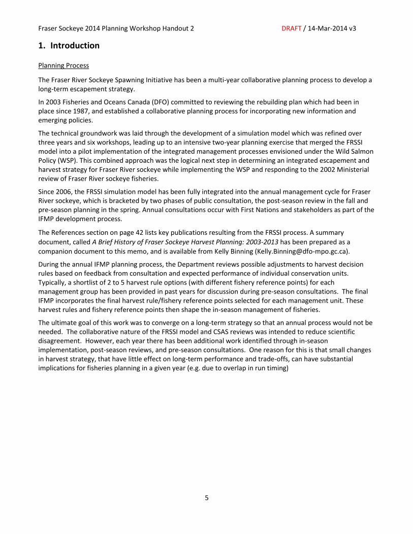
The Fraser River Sockeye Spawning Initiative has been a multi-year collaborative planning process to develop a long-term escapement strategy.
In 2003 Fisheries and Oceans Canada (DFO) committed to reviewing the rebuilding plan which had been in place since 1987, and established a collaborative planning process for incorporating new information and emerging policies.
The technical groundwork was laid through the development of a simulation model which was refined over three years and six workshops, leading up to an intensive two-year planning exercise that merged the FRSSI model into a pilot implementation of the integrated management processes envisioned under the Wild Salmon Policy (WSP). This combined approach was the logical next step in determining an integrated escapement and harvest strategy for Fraser River sockeye while implementing the WSP and responding to the 2002 Ministerial review of Fraser River sockeye fisheries.
Since 2006, the FRSSI simulation model has been fully integrated into the annual management cycle for Fraser River sockeye, which is bracketed by two phases of public consultation, the post-season review in the fall and pre-season planning in the spring. Annual consultations occur with First Nations and stakeholders as part of the IFMP development process.
The References section on page 42 lists key publications resulting from the FRSSI process. A summary
document, called A Brief History of Fraser Sockeye Harvest Planning: 2003-2013 has been prepared as a
companion document to this memo, and is available from Kelly Binning ([email protected]).
During the annual IFMP planning process, the Department reviews possible adjustments to harvest decision rules based on feedback from consultation and expected performance of individual conservation units. Typically, a shortlist of 2 to 5 harvest rule options (with different fishery reference points) for each management group has been provided in past years for discussion during pre-season consultations. The final IFMP incorporates the final harvest rule/fishery reference points selected for each management unit. These harvest rules and fishery reference points then shape the in-season management of fisheries.
The ultimate goal of this work was to converge on a long-term strategy so that an annual process would not be needed. The collaborative nature of the FRSSI model and CSAS reviews was intended to reduce scientific disagreement. However, each year there has been additional work identified through in-season implementation, post-season reviews, and pre-season consultations. One reason for this is that small changes in harvest strategy, that have little effect on long-term performance and trade-offs, can have substantial implications for fisheries planning in a given year (e.g. due to overlap in run timing)
Fraser Sockeye 2014 Planning Workshop Handout 2 DRAFT / 14-Mar-2014 v3
6
Expectations for 2014
The 2014 pre-season forecast generally predicts (three in four chance) of an above cycle average return, given the large total spawner abundance in the 2010 brood year for a number of stocks; survival (recruits-per-spawner) has returned to average generally for most stocks following the 2009 poor returns (amongst the lowest survival on record for most stocks). However, there are stock-specific differences in forecasted abundance that need to be considered in the planning and implementation of fisheries
Major challenges for 2014 harvest planning are:
Uncertainty in forecasts: Higher than usual, because for several of the stocks the brood year abundance exceeded the previously observed range, and there is no available data on returns from these abundances (Scotch, Seymour, Harrison, Late Shuswap and Portage Creek). ). Although juvenile data do provide support for the overcompensation (lower freshwater survival) predicted by adult stock-recruitment models. Note that the Chilko does not fall into this category, because the forecast is based on smolt data, which did not fall outside the observed range.
Uncertain en-route mortality: Fraser sockeye can experience substantial mortality during their upstream migration, depending on river conditions (water temperature and discharge) and timing of peak migration. This en-route mortality occurs upstream of most of the major fisheries, and in-season projections of mortality are used to adjust the allowable exploitation rate in an attempt to achieve escapement objectives. The adjustments tend to be small for Summer Run sockeye (except for 1998, 2006 and 2013), but can be substantial for the other management groups (e.g. 20-30%, out of a total allowable mortality of 60%)
Availability of in-season information: In-season estimates of abundance are generated for the management groups and larger stocks with current stock ID methodology (i.e. scale patterns, DNA). Estimates become better as more of the stocks migrate past the major fisheries and enter the river, and weekly in-season run size updates/modifications typically occur shortly after the peak migration of each management group through Area 20.
Aggregate harvest of multiple stocks: Populations of Fraser Sockeye differ in terms of their productivity, which also changes over time. In past years, the aggregate harvest plan has been constrained to 60% total allowable mortality to protect less productive stocks in a management group. One option for 2014, given the large expected run size, is to increase the cap to 65%.
Uncertainty in capacity: Given all of the challenges listed above, it is likely that spawner abundances in 2014 will be large to very large for several of the stocks. This raises concerns regarding potential capacity limits of the nursery lakes, but it is difficult to estimate optimal levels of spawner abundance, either as a long-term average or for a specific year. Alternative estimates can differ widely, and this uncertainty needs to be taken into account (e.g. when planning ESSR-type fisheries).
Based on these challenges, DFO has included 2 options in the draft Integrated Fisheries Management Plan:
Option 1 – Like Cycle Year: Same TAM rules as in 2010, except that the Fishery Reference Points were adjusted to account for Raft now being managed as part of the Summer group, and Harrison and North Thompson being managed as miscellaneous Summer stocks. In addition the Early Stuart Fishery Reference Points were changed to those used durting the last two years.
Option 2 – Increase TAM cap: Increase TAM cap to 65% due to large expected run size for Early Summer, Summers and Lates. Lower FRP stay the same, but Upper FRP increase due to the gradual increase in TAM until it reaches the cap.
Chapter 2 of this memo summarizes the planning context for 2014, in terms of recent spawner abundances, patterns in productivity, and integrated biological status. Chapter 3 describes the 2 options in detail and

Fraser Sockeye 2014 Planning Workshop Handout 2 DRAFT / 14-Mar-2014 v3
7
compares their expected outcomes, given pre-season estimates of abundance and en-route mortality. Chapter 4 outlines additional considerations that are likely to shape the 2014 fishing season.
Fraser Sockeye 2014 Planning Workshop Handout 2 DRAFT / 14-Mar-2014 v3
8
2. Context for 2014 Planning
Overview
This Chapter covers 3 topics:
Recent spawner abundances compared to the observed range (by stock)
Indications of improved productivity (total)
Integrated biological status under the Wild Salmon Policy (by of conservation unit)
Recent spawner abundances compared to observed time series and to various benchmarks
The FRSSI model is useful for evaluating the long-term expected performance of alternative strategies. This section looks at the other side of the equation: What is the observed performance of the recent harvest strategies in terms of spawner abundance?
Table 1 to Table 3 summarize observed spawner abundances for the 19 modelled stocks and show comparisons in different contexts.
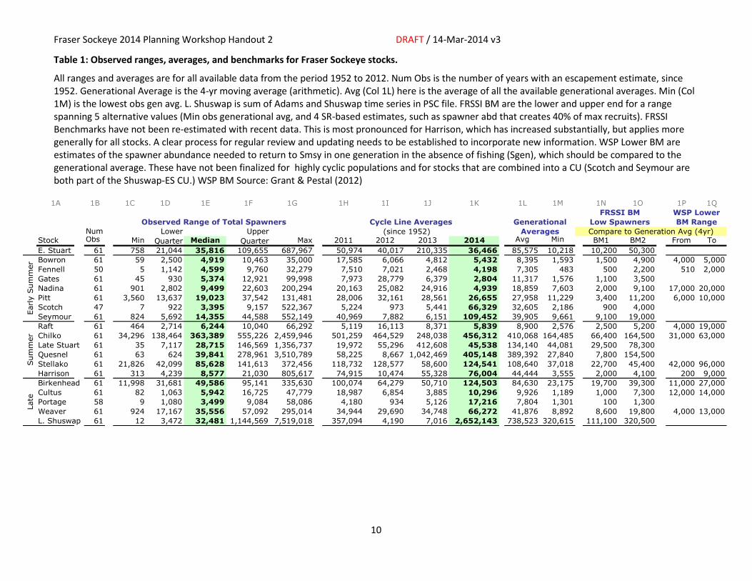
Key points to note in Table 1 are:
Fraser sockeye stocks cover a very wide range of abundances. Median spawner abundances since 1952 range from less than 10,000 (Bowron, Fennel, Gates, Nadina, Scotch, Raft, Harrison, Cultus, Portage) to more than 300,000 (Chilko). (Col 1E)
Fraser sockeye stocks fluctuate greatly over time. The largest observed spawner abundance (Col 1G) is typically many times larger than the median (as high as 150 times for Scotch and 230 times for Late Shuswap). Figure 11 (p35) and Figure 12 (p36) show the patterns over time.
Some of the stocks, which typically account for a large part of the annual abundance, show strong cyclic patterns, with the dominant years 10 to 100 times larger than the off-cycle years (Cols 1H to 1K).
Even the generational averages, which smooth out the annual fluctuations and cyclic pattern, are highly variable over time (compare min in Col 1M to avg in Col 1L).
Note: The generational average used throughout the tables and figures in this memo is the arithmetic 4yr mean calculated as A+B+C+D/4. This is more sensitive to large outliers than the geometric mean calculated as Root(A*B*C*D), but the resulting values are more in line with the common interpretation of a central value. This makes the most difference for cyclic stocks. To illustrate for 2009 to 2012:
Stock Spawners Arithmetic Mean Geometric Mean
Stellako 27,793 / 204,414 / 85,628/ 137,993
113,957 90,517
Late Shuswap 32,481 / 7,519,018 / 165,695 / 12
1,929,302 26,398
Fraser Sockeye 2014 Planning Workshop Handout 2 DRAFT / 14-Mar-2014 v3
9
Two sets of benchmarks have been used to evaluate Fraser River Sockeye. The FRSSI BM for all stocks (source= Pestal, Huang and Cass 2011) and the WSP BM for non-cyclic stocks (source = Grant and Pestal 2012). These are listed in columns 1N to 1Q.
o The two sets of benchmarks cover a similar range for 5 of the 11 stocks (Bowron, Fennel, Pitt, Harrison, Weaver). But note that both sets of benchmarks are outdated for Harrison, given recent spawner abundances.
o WSP lower BM are roughly half the FRSSI BM 2 for 2 of the stocks (Chilko, Birkenhead).
o WSP lower BM are roughly double the FRSSI BM 2 for 3 of the stocks (Nadina, Stellako, Cultus).
o WSP lower BM is roughly 4 times the FRSSI BM 2 for Raft.
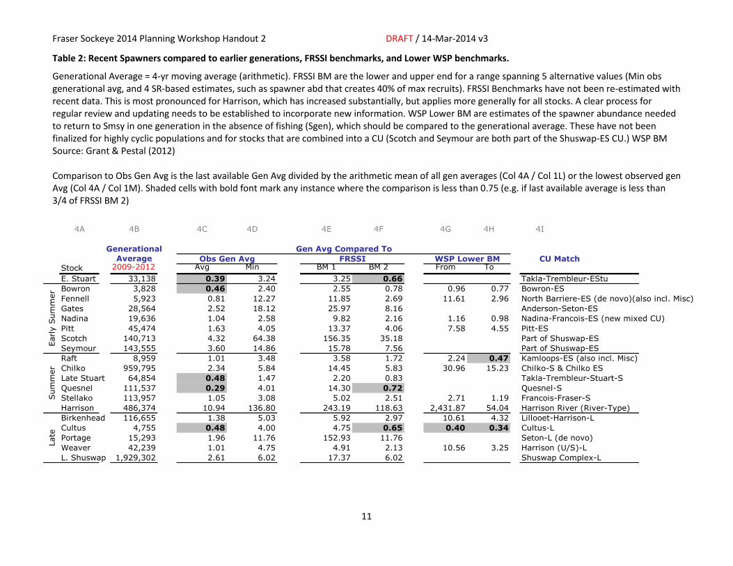
Key points to note in Table 2 are:
For 14 of the 19 stocks, the most recent generational average (2009-2012) is close to or larger than the average of all the observed generational averages (Col 4C). The exceptions are Early Stuart, Bowron, Late Stuart, Quesnel, and Cultus. For all stocks, the latest gen avg is larger than their lowest observed generational average (Col 4D).
For 16 of the 19 stocks, the most recent generational average (2009-2012) is close to or larger than the FRSSI Benchmark 2, which has been used to identify low spawner abundance (Col 4F). The exceptions are Early Stuart, Quesnel, and Cultus.
Lower WSP benchmarks have been developed for 11 stocks without persistent cyclic patterns. For 10 of the 11 stocks with WSP BM, the most recent generational average (2009-2012) is close to or larger than the lower end of the uncertainty range in BM estimates (Col 4G). The exception is Cultus. ). 8 of 11 stocks are at or above the upper end of the uncertainty range for the Lower WSP BM (Col 4H). The exceptions are Bowron, Raft, and Cultus.
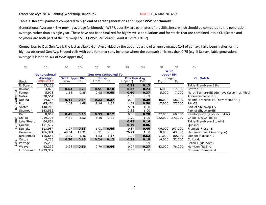
Key points to note in Table 3 are:
Despite the large spawner abundance in 2010, the most recent generational average (2009-2012) falls below the highest observed generational average for 12 of the 19 stock (shaded grey in Col 5H), and is smaller than the upper quarter of the observed generational averages for 6 stocks (shaded grey in Col 5G).
For 5 of the stocks, the most recent generational average (2009-2012) was the highest observed generational average since 1955 (as marked by 1.00 in Col 5H). These stocks are Scotch, Seymour, Chilko, Harrison, and Late Shuswap.
For 6 stocks of the 11 non-cyclic stocks for which WSP BM are available, the most recent generational average (2009-2012) is substantially below the upper end of the range of estimates for the Upper WSP BM (shaded in Col 5D).
Fraser Sockeye 2014 Planning Workshop Handout 2 DRAFT / 14-Mar-2014 v3
10
Table 1: Observed ranges, averages, and benchmarks for Fraser Sockeye stocks.
All ranges and averages are for all available data from the period 1952 to 2012. Num Obs is the number of years with an escapement estimate, since 1952. Generational Average is the 4-yr moving average (arithmetic). Avg (Col 1L) here is the average of all the available generational averages. Min (Col 1M) is the lowest obs gen avg. L. Shuswap is sum of Adams and Shuswap time series in PSC file. FRSSI BM are the lower and upper end for a range spanning 5 alternative values (Min obs generational avg, and 4 SR-based estimates, such as spawner abd that creates 40% of max recruits). FRSSI Benchmarks have not been re-estimated with recent data. This is most pronounced for Harrison, which has increased substantially, but applies more generally for all stocks. A clear process for regular review and updating needs to be established to incorporate new information. WSP Lower BM are estimates of the spawner abundance needed to return to Smsy in one generation in the absence of fishing (Sgen), which should be compared to the generational average. These have not been finalized for highly cyclic populations and for stocks that are combined into a CU (Scotch and Seymour are both part of the Shuswap-ES CU.) WSP BM Source: Grant & Pestal (2012)
1A 1B 1C 1D 1E 1F 1G 1H 1I 1J 1K 1L 1M 1N 1O 1P 1Q
TABLE 1: BENCHMARK SUMMARY
v1 2014-02-25
Num
Stock Obs Min Median Max 2011 2012 2013 2014 Avg Min BM1 BM2 From To
E. Stuart 61 758 21,044 35,816 109,655 687,967 50,974 40,017 210,335 36,466 85,575 10,218 10,200 50,300
Bowron 61 59 2,500 4,919 10,463 35,000 17,585 6,066 4,812 5,432 8,395 1,593 1,500 4,900 4,000 5,000
Fennell 50 5 1,142 4,599 9,760 32,279 7,510 7,021 2,468 4,198 7,305 483 500 2,200 510 2,000
Gates 61 45 930 5,374 12,921 99,998 7,973 28,779 6,379 2,804 11,317 1,576 1,100 3,500
Nadina 61 901 2,802 9,499 22,603 200,294 20,163 25,082 24,916 4,939 18,859 7,603 2,000 9,100 17,000 20,000
Pitt 61 3,560 13,637 19,023 37,542 131,481 28,006 32,161 28,561 26,655 27,958 11,229 3,400 11,200 6,000 10,000
Scotch 47 7 922 3,395 9,157 522,367 5,224 973 5,441 66,329 32,605 2,186 900 4,000
Seymour 61 824 5,692 14,355 44,588 552,149 40,969 7,882 6,151 109,452 39,905 9,661 9,100 19,000
Raft 61 464 2,714 6,244 10,040 66,292 5,119 16,113 8,371 5,839 8,900 2,576 2,500 5,200 4,000 19,000
Chilko 61 34,296 138,464 363,389 555,226 2,459,946 501,259 464,529 248,038 456,312 410,068 164,485 66,400 164,500 31,000 63,000
Late Stuart 61 35 7,117 28,715 146,569 1,356,737 19,972 55,296 412,608 45,538 134,140 44,081 29,500 78,300
Quesnel 61 63 624 39,841 278,961 3,510,789 58,225 8,667 1,042,469 405,148 389,392 27,840 7,800 154,500
Stellako 61 21,826 42,099 85,628 141,613 372,456 118,732 128,577 58,600 124,541 108,640 37,018 22,700 45,400 42,000 96,000
Harrison 61 313 4,239 8,577 21,030 805,617 74,915 10,474 55,328 76,004 44,444 3,555 2,000 4,100 200 9,000
Birkenhead 61 11,998 31,681 49,586 95,141 335,630 100,074 64,279 50,710 124,503 84,630 23,175 19,700 39,300 11,000 27,000
Cultus 61 82 1,063 5,942 16,725 47,779 18,987 6,854 3,885 10,296 9,926 1,189 1,000 7,300 12,000 14,000
Portage 58 9 1,080 3,499 9,084 58,086 4,180 934 5,126 17,216 7,804 1,301 100 1,300
Weaver 61 924 17,167 35,556 57,092 295,014 34,944 29,690 34,748 66,272 41,876 8,892 8,600 19,800 4,000 13,000
L. Shuswap 61 12 3,472 32,481 1,144,569 7,519,018 357,094 4,190 7,016 2,652,143 738,523 320,615 111,100 320,500
Compare to Generation Avg (4yr)
Generational
Averages
Late
Sum
mer
Observed Range of Total Spawners
Lower
Quarter
Upper
Quarter
Early S
um
mer
Cycle Line Averages
(since 1952)
FRSSI BM
Low Spawners
WSP Lower
BM Range
Fraser Sockeye 2014 Planning Workshop Handout 2 DRAFT / 14-Mar-2014 v3
11
Table 2: Recent Spawners compared to earlier generations, FRSSI benchmarks, and Lower WSP benchmarks.
Generational Average = 4-yr moving average (arithmetic). FRSSI BM are the lower and upper end for a range spanning 5 alternative values (Min obs generational avg, and 4 SR-based estimates, such as spawner abd that creates 40% of max recruits). FRSSI Benchmarks have not been re-estimated with recent data. This is most pronounced for Harrison, which has increased substantially, but applies more generally for all stocks. A clear process for regular review and updating needs to be established to incorporate new information. WSP Lower BM are estimates of the spawner abundance needed to return to Smsy in one generation in the absence of fishing (Sgen), which should be compared to the generational average. These have not been finalized for highly cyclic populations and for stocks that are combined into a CU (Scotch and Seymour are both part of the Shuswap-ES CU.) WSP BM Source: Grant & Pestal (2012) Comparison to Obs Gen Avg is the last available Gen Avg divided by the arithmetic mean of all gen averages (Col 4A / Col 1L) or the lowest observed gen Avg (Col 4A / Col 1M). Shaded cells with bold font mark any instance where the comparison is less than 0.75 (e.g. if last available average is less than 3/4 of FRSSI BM 2)
4A 4B 4C 4D 4E 4F 4G 4H 4I
Generational
Average
Stock 2009-2012 Avg Min BM 1 BM 2 From To
E. Stuart 33,138 0.39 3.24 3.25 0.66 Takla-Trembleur-EStu
Bowron 3,828 0.46 2.40 2.55 0.78 0.96 0.77 Bowron-ES
Fennell 5,923 0.81 12.27 11.85 2.69 11.61 2.96 North Barriere-ES (de novo)(also incl. Misc)
Gates 28,564 2.52 18.12 25.97 8.16 Anderson-Seton-ES
Nadina 19,636 1.04 2.58 9.82 2.16 1.16 0.98 Nadina-Francois-ES (new mixed CU)
Pitt 45,474 1.63 4.05 13.37 4.06 7.58 4.55 Pitt-ES
Scotch 140,713 4.32 64.38 156.35 35.18 Part of Shuswap-ES
Seymour 143,555 3.60 14.86 15.78 7.56 Part of Shuswap-ES
Raft 8,959 1.01 3.48 3.58 1.72 2.24 0.47 Kamloops-ES (also incl. Misc)
Chilko 959,795 2.34 5.84 14.45 5.83 30.96 15.23 Chilko-S & Chilko ES
Late Stuart 64,854 0.48 1.47 2.20 0.83 Takla-Trembleur-Stuart-S
Quesnel 111,537 0.29 4.01 14.30 0.72 Quesnel-S
Stellako 113,957 1.05 3.08 5.02 2.51 2.71 1.19 Francois-Fraser-S
Harrison 486,374 10.94 136.80 243.19 118.63 2,431.87 54.04 Harrison River (River-Type)
Birkenhead 116,655 1.38 5.03 5.92 2.97 10.61 4.32 Lillooet-Harrison-L
Cultus 4,755 0.48 4.00 4.75 0.65 0.40 0.34 Cultus-L
Portage 15,293 1.96 11.76 152.93 11.76 Seton-L (de novo)
Weaver 42,239 1.01 4.75 4.91 2.13 10.56 3.25 Harrison (U/S)-L
L. Shuswap 1,929,302 2.61 6.02 17.37 6.02 Shuswap Complex-L
Early S
um
mer
Sum
mer
Late
Gen Avg Compared To
CU MatchWSP Lower BM FRSSIObs Gen Avg
Fraser Sockeye 2014 Planning Workshop Handout 2 DRAFT / 14-Mar-2014 v3
12
Table 3: Recent Spawners compared to high end of earlier generations and Upper WSP benchmarks.
Generational Average = 4-yr moving average (arithmetic). WSP Upper BM are estimates of the 80% Smsy, which should be compared to the generation
average, rather than a single year. These have not been finalized for highly cyclic populations and for stocks that are combined into a CU (Scotch and
Seymour are both part of the Shuswap-ES CU.) WSP BM Source: Grant & Pestal (2012)
Comparison to Obs Gen Avg is the last available Gen Avg divided by the upper quartile of all gen averages (1/4 of gen avg have been higher) or the
highest observed Gen Avg. Shaded cells with bold font mark any instance where the comparison is less than 0.75 (e.g. if last available generational
average is less than 3/4 of WSP Upper BM)
5A 5B 5C 5D 5E 5F 5G 5H 5I 5J 5K
Generational
Average
Stock 2009-2012 From To From To Upper Q Max From To
E. Stuart 33,138 0.32 0.13 Takla-Trembleur-EStu
Bowron 3,828 0.64 0.23 0.51 0.18 0.37 0.24 6,000 17,000 Bowron-ES
Fennell 5,923 1.18 0.85 0.95 0.68 0.60 0.37 5,000 7,000 North Barriere-ES (de novo)(also incl. Misc)
Gates 28,564 1.56 0.89 Anderson-Seton-ES
Nadina 19,636 0.41 0.34 0.33 0.27 0.97 0.29 48,000 58,000 Nadina-Francois-ES (new mixed CU)
Pitt 45,474 2.67 1.68 2.14 1.35 1.59 0.50 17,000 27,000 Pitt-ES
Scotch 140,713 5.01 1.00 Part of Shuswap-ES
Seymour 143,555 3.83 1.00 Part of Shuswap-ES
Raft 8,959 0.41 0.15 0.33 0.12 0.88 0.28 22,000 60,000 Kamloops-ES (also incl. Misc)
Chilko 959,795 4.32 3.52 3.46 2.81 1.72 1.00 222,000 273,000 Chilko-S & Chilko ES
Late Stuart 64,854 0.43 0.16 Takla-Trembleur-Stuart-S
Quesnel 111,537 0.19 0.06 Quesnel-S
Stellako 113,957 1.27 0.58 1.01 0.46 0.87 0.46 90,000 197,000 Francois-Fraser-S
Harrison 486,374 48.64 11.31 38.91 9.05 26.44 1.00 10,000 43,000 Harrison River (River-Type)
Birkenhead 116,655 2.29 1.46 1.83 1.17 1.03 0.52 51,000 80,000 Lillooet-Harrison-L
Cultus 4,755 0.30 0.15 0.24 0.12 0.32 0.18 16,000 32,000 Cultus-L
Portage 15,293 1.56 0.99 Seton-L (de novo)
Weaver 42,239 0.98 0.56 0.79 0.44 0.77 0.37 43,000 76,000 Harrison (U/S)-L
L. Shuswap 1,929,302 2.30 1.00 Shuswap Complex-L
Early S
um
mer
Sum
mer
Late
RangeWSP Upper BM Smsy Obs Gen Avg
WSP
Upper BM
CU Match
Gen Avg Compared To
Fraser Sockeye 2014 Planning Workshop Handout 2 DRAFT / 14-Mar-2014 v3
13
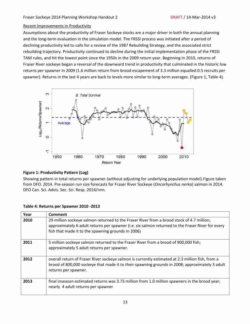
Recent Improvements in Productivity
Assumptions about the productivity of Fraser Sockeye stocks are a major driver in both the annual planning
and the long-term evaluation in the simulation model. The FRSSI process was initiated after a period of
declining productivity led to calls for a review of the 1987 Rebuilding Strategy, and the associated strict
rebuilding trajectory. Productivity continued to decline during the initial implementation phase of the FRSSI
TAM rules, and hit the lowest point since the 1950s in the 2009 return year. Beginning in 2010, returns of
Fraser River sockeye began a reversal of the downward trend in productivity that culminated in the historic low
returns per spawner in 2009 (1.6 million return from brood escapement of 3.3 million equalled 0.5 recruits per
spawner). Returns in the last 4 years are back to levels more similar to long-term averages. (Figure 1, Table 4).
Figure 1: Productivity Pattern (Log)
Showing pattern in total returns per spawner (without adjusting for underlying population model).Figure taken from DFO. 2014. Pre-season run size forecasts for Fraser River Sockeye (Oncorhynchus nerka) salmon in 2014. DFO Can. Sci. Advis. Sec. Sci. Resp. 2014/nnn. Table 4: Returns per Spawner 2010 -2013
Year Comment
2010 29 million sockeye salmon returned to the Fraser River from a brood stock of 4.7 million; approximately 6 adult returns per spawner (i.e. six salmon returned to the Fraser River for every fish that made it to the spawning grounds in 2006)
2011 5 million sockeye salmon returned to the Fraser River from a brood of 900,000 fish; approximately 5 adult returns per spawner.
2012 overall return of Fraser River sockeye salmon is currently estimated at 2.3 million fish, from a brood of 800,000 sockeye that made it to their spawning grounds in 2008; approximately 3 adult returns per spawner.
2013 final inseason estimated returns was 3.73 million from 1.0 million spawners in the brood year; nearly 4 adult returns per spawner
Fraser Sockeye 2014 Planning Workshop Handout 2 DRAFT / 14-Mar-2014 v3
14
Integrated Biological Status Under Wild Salmon Policy
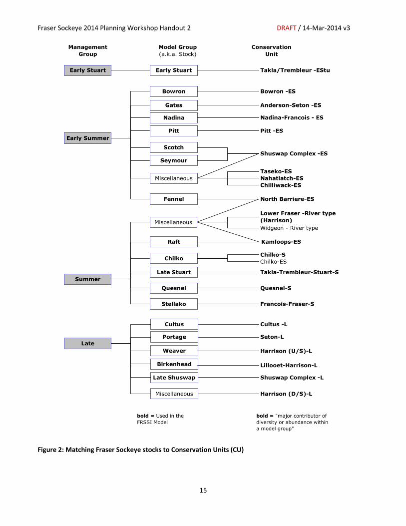
A key element of the Wild Salmon Policy (DFO 2005) is a formal status evaluation of conservation units.
Sockeye conservation units are generally based on rearing lake and migration timing, and for Fraser sockeye,
stocks and conservation units line up closely (Figure 2). The WSP defines 3 status zones (Red / Amber / Green),
and describes assessment actions and management considerations for each zone (DFO 2005)
The biological status of Fraser River sockeye conservation units was assessed through an expert-based process
in 2011 (Grant and Pestal 2012). Evaluations of integrated status took into account three formal status metrics
(abundance relative to WSP benchmarks, long-term trend, and short-term trend) as well as additional
information (absolute abundance, data quality, patterns of exploitation rate).
Note that these status evaluations were based on information up to the 2010 return year, but also note that
the individual metrics are designed to be robust to annual fluctuations (e.g. using generational averages)
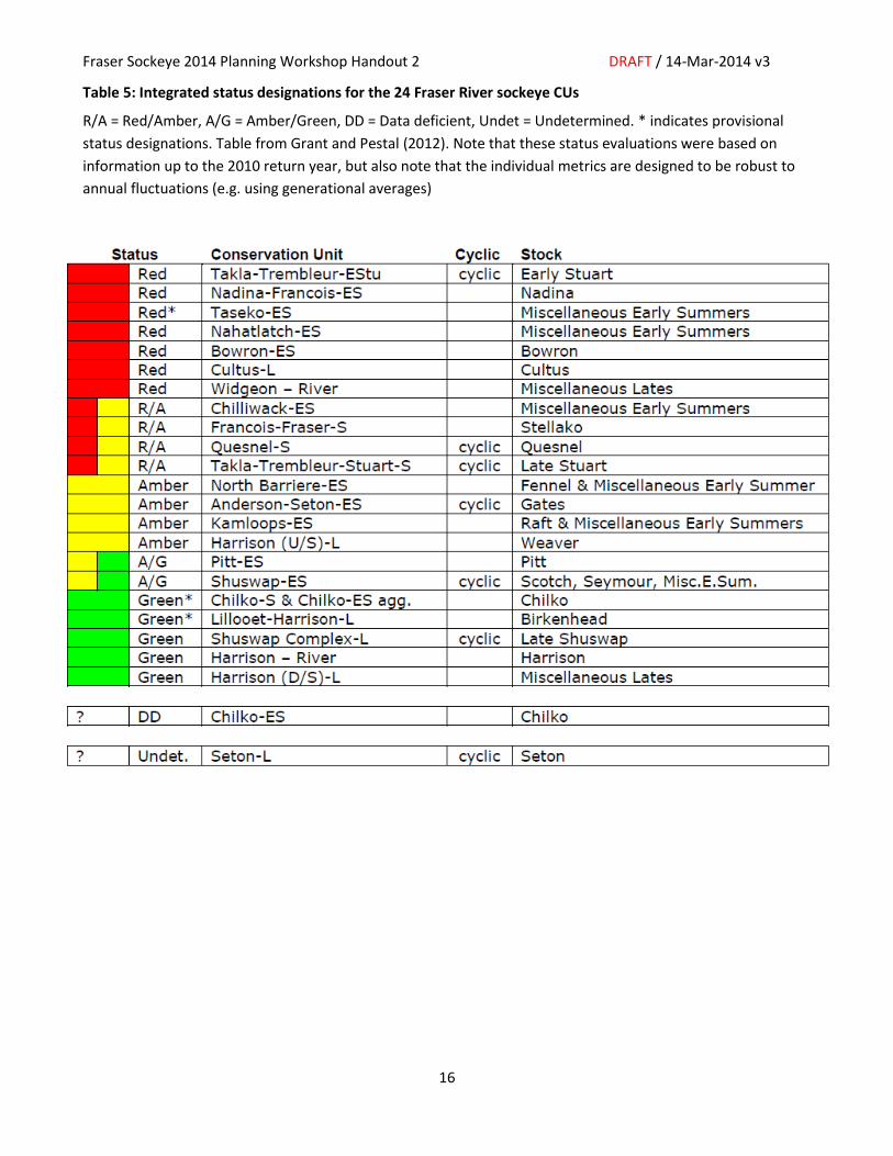
Final integrated status for each of the 24 Fraser Sockeye CUs included the following: seven Red, four
Red/Amber, four Amber, two Amber/Green, five Green, one Data Deficient, and one Undetermined (Table 5).
Detailed status results for each of the groups and expert commentary (which identified key metrics and
associated data that guided these status determinations) are published separately (Appendix 2 of Grant and
Pestal 2012), and are necessary for CU status interpretation in WSP Strategy 4.
Integrated status determination for cyclic CUs presented the largest challenge to participants. Specifically, the
appropriate method for estimating benchmarks for the relative-abundance metric of cyclic CUs was debated.
Since this issue could not be resolved at the workshop, these metrics for cyclic CUs were excluded from status
evaluations. However, the group felt that there remained sufficient data for status evaluations, particularly
when compared to other non-Fraser Sockeye CUs, to assess status for cyclic CUs. The unique population
dynamics of these CUs further added complexity to cyclic CU status evaluations.
Note that the WSP Benchmarks for Relative Abundance are not management references points (i.e. not
designed to trigger specific annual harvest measures). Rather, they are intended as part of an integrated status
evaluation.
Fraser Sockeye 2014 Planning Workshop Handout 2 DRAFT / 14-Mar-2014 v3
15
Figure 2: Matching Fraser Sockeye stocks to Conservation Units (CU)
Management
Group
Model Group
(a.k.a. Stock)
Conservation
Unit
Early Stuart
Early Summer
Summer
Late
Early Stuart Takla/Trembleur -EStu
Bowron
Nadina
Gates
Fennel
Raft
Pitt
Scotch
Seymour
bold = "major contributor of
diversity or abundance within
a model group"
bold = Used in the
FRSSI Model
Miscellaneous
Bowron -ES
Anderson-Seton -ES
North Barriere-ES
Nadina-Francois - ES
Pitt -ES
Shuswap Complex -ES
Taseko-ES
Nahatlatch-ES
Chilliwack-ES
Chilko
Quesnel
Late Stuart
Stellako
Chilko-S
Chilko-ES
Takla-Trembleur-Stuart-S
Quesnel-S
Francois-Fraser-S
Cultus
Late Shuswap
Miscellaneous
Weaver
Birkenhead
Portage
Miscellaneous
Widgeon - River type
Harrison (D/S)-L
Cultus -L
Lower Fraser -River type
(Harrison)
Shuswap Complex -L
Seton-L
Harrison (U/S)-L
Lillooet-Harrison-L
Kamloops-ES
Fraser Sockeye 2014 Planning Workshop Handout 2 DRAFT / 14-Mar-2014 v3
16
Table 5: Integrated status designations for the 24 Fraser River sockeye CUs
R/A = Red/Amber, A/G = Amber/Green, DD = Data deficient, Undet = Undetermined. * indicates provisional
status designations. Table from Grant and Pestal (2012). Note that these status evaluations were based on
information up to the 2010 return year, but also note that the individual metrics are designed to be robust to
annual fluctuations (e.g. using generational averages)
Fraser Sockeye 2014 Planning Workshop Handout 2 DRAFT / 14-Mar-2014 v3
17
3. Proposed Options for 2014
Overview
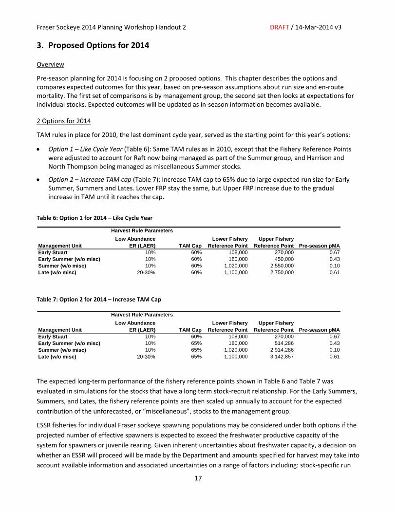
Pre-season planning for 2014 is focusing on 2 proposed options. This chapter describes the options and compares expected outcomes for this year, based on pre-season assumptions about run size and en-route mortality. The first set of comparisons is by management group, the second set then looks at expectations for individual stocks. Expected outcomes will be updated as in-season information becomes available.
2 Options for 2014
TAM rules in place for 2010, the last dominant cycle year, served as the starting point for this year’s options:
Option 1 – Like Cycle Year (Table 6): Same TAM rules as in 2010, except that the Fishery Reference Points were adjusted to account for Raft now being managed as part of the Summer group, and Harrison and North Thompson being managed as miscellaneous Summer stocks.
Option 2 – Increase TAM cap (Table 7): Increase TAM cap to 65% due to large expected run size for Early Summer, Summers and Lates. Lower FRP stay the same, but Upper FRP increase due to the gradual increase in TAM until it reaches the cap.
Table 6: Option 1 for 2014 – Like Cycle Year
Table 7: Option 2 for 2014 – Increase TAM Cap
The expected long-term performance of the fishery reference points shown in Table 6 and Table 7 was
evaluated in simulations for the stocks that have a long term stock-recruit relationship. For the Early Summers,
Summers, and Lates, the fishery reference points are then scaled up annually to account for the expected
contribution of the unforecasted, or “miscellaneous”, stocks to the management group.
ESSR fisheries for individual Fraser sockeye spawning populations may be considered under both options if the
projected number of effective spawners is expected to exceed the freshwater productive capacity of the
system for spawners or juvenile rearing. Given inherent uncertainties about freshwater capacity, a decision on
whether an ESSR will proceed will be made by the Department and amounts specified for harvest may take into
account available information and associated uncertainties on a range of factors including: stock-specific run
Harvest Rule Parameters
Low Abundance
ER (LAER) TAM Cap
Lower Fishery
Reference Point
Upper Fishery
Reference Point Pre-season pMA
Early Stuart 10% 60% 108,000 270,000 0.67
Early Summer (w/o misc) 10% 65% 180,000 514,286 0.43
Summer (w/o misc) 10% 65% 1,020,000 2,914,286 0.10
Late (w/o misc) 20-30% 65% 1,100,000 3,142,857 0.61
Management Unit
Harvest Rule Parameters
Low Abundance
ER (LAER) TAM Cap
Lower Fishery
Reference Point
Upper Fishery
Reference Point Pre-season pMA
Early Stuart 10% 60% 108,000 270,000 0.67
Early Summer (w/o misc) 10% 60% 180,000 450,000 0.43
Summer (w/o misc) 10% 60% 1,020,000 2,550,000 0.10
Late (w/o misc) 20-30% 60% 1,100,000 2,750,000 0.61
Management Unit
Fraser Sockeye 2014 Planning Workshop Handout 2 DRAFT / 14-Mar-2014 v3
18
size, projected spawner abundances, productive capacity of the system, stock composition in fishing area, and
selectivity of fishing gear. Given uncertainties in in-season information, the Department may permit only a
portion of any estimated surplus to be harvested. See section 6.1 of the IFMP for general information on ESSR
fisheries. Chapter 4 of this memo has some additional information about capacity estimates and considerations
that would shape potential ESSR fisheries.
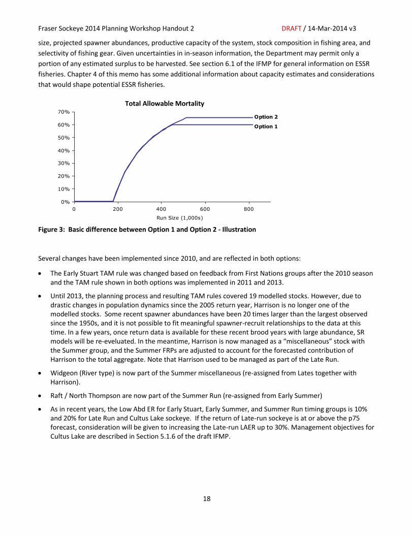
Figure 3: Basic difference between Option 1 and Option 2 - Illustration
Several changes have been implemented since 2010, and are reflected in both options:
The Early Stuart TAM rule was changed based on feedback from First Nations groups after the 2010 season and the TAM rule shown in both options was implemented in 2011 and 2013.
Until 2013, the planning process and resulting TAM rules covered 19 modelled stocks. However, due to drastic changes in population dynamics since the 2005 return year, Harrison is no longer one of the modelled stocks. Some recent spawner abundances have been 20 times larger than the largest observed since the 1950s, and it is not possible to fit meaningful spawner-recruit relationships to the data at this time. In a few years, once return data is available for these recent brood years with large abundance, SR models will be re-eveluated. In the meantime, Harrison is now managed as a “miscellaneous” stock with the Summer group, and the Summer FRPs are adjusted to account for the forecasted contribution of Harrison to the total aggregate. Note that Harrison used to be managed as part of the Late Run.
Widgeon (River type) is now part of the Summer miscellaneous (re-assigned from Lates together with Harrison).
Raft / North Thompson are now part of the Summer Run (re-assigned from Early Summer)
As in recent years, the Low Abd ER for Early Stuart, Early Summer, and Summer Run timing groups is 10% and 20% for Late Run and Cultus Lake sockeye. If the return of Late-run sockeye is at or above the p75 forecast, consideration will be given to increasing the Late-run LAER up to 30%. Management objectives for Cultus Lake are described in Section 5.1.6 of the draft IFMP.
Option 1
Option 2
0%
10%
20%
30%
40%
50%
60%
70%
0 200 400 600 800
Run Size (1,000s)
Total Allowable Mortality
Fraser Sockeye 2014 Planning Workshop Handout 2 DRAFT / 14-Mar-2014 v3
19
Comparing Expected Outcomes for Options 1 and 2 – By Management Group
Actual outcomes for the harvest strategy will depend strongly on the observed run size, implementation of the
fishing plan, and observed en-route mortality.
Table 9 to Table 12 show the range of expected outcomes (i.e. exploitation rates, available harvest, and
expected numbers of spawners to the grounds) under each of the 2 options for the plausible range of
abundance forecast and a pre-season management adjustment to account for migration conditions and
associated en-route mortality. For pre-season planning purposes, proportional management adjustments
(pMAs) used for illustration are:
Early Stuart: median of the long term pMA dataset to 2012.
Early Summer: median of the Scotch-Seymour dominant and subdominant pMA dataset to 2012
Summer: median of the long term pMA dataset to 2012
Lates – for the Birkenhead component, the median of the long term pMA dataset to 2012. For the remainder of the Late run: the average of a) the median of the Adams dominant and subdominant pMA dataset to 2012 and b) the modelled pMA based on in-river timing predictions.
The pMAs for Early Stuart, Early Summer, Summer and Late Run sockeye will likely change in-season with
updated information on environmental conditions and migration timing. The pre-season pMA and method for
determining pMA for Late Run in 2014 has yet to be decided. The pre-season pMA values for all management
groups will continue to be reviewed and updated by the Fraser Panel prior to the start of the fishing season.
The “MA” (management adjustment) values in the tables are the escapement goals multiplied by the pMA.
The Fraser Panel will review MA models with particular emphasis on understanding the sources of bias in
forecasts of river temperatures, potential alternative models and approaches including models based on
subsets of years and/or component stocks, and conceptual approaches to quantifying the relative impacts of
measure error and en-route mortality.
Note that these values do not take into account the pre-spawn mortality which can occur after spawners reach
the grounds. We currently do not have any methods to predict pre-spawn mortality rates. Table 8 describes the
types of information shown in Table 9 to Table 12.
Key points to note in the aggregate projections:
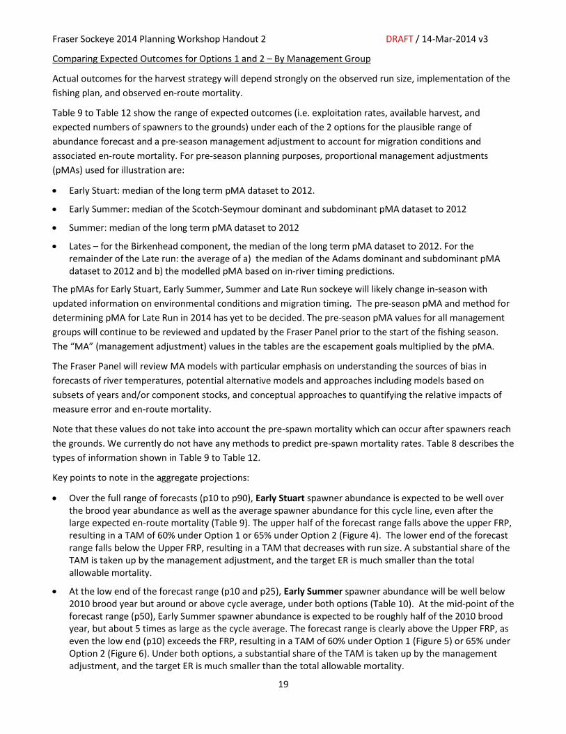
Over the full range of forecasts (p10 to p90), Early Stuart spawner abundance is expected to be well over the brood year abundance as well as the average spawner abundance for this cycle line, even after the large expected en-route mortality (Table 9). The upper half of the forecast range falls above the upper FRP, resulting in a TAM of 60% under Option 1 or 65% under Option 2 (Figure 4). The lower end of the forecast range falls below the Upper FRP, resulting in a TAM that decreases with run size. A substantial share of the TAM is taken up by the management adjustment, and the target ER is much smaller than the total allowable mortality.
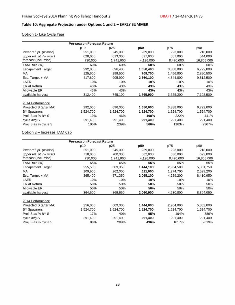
At the low end of the forecast range (p10 and p25), Early Summer spawner abundance will be well below 2010 brood year but around or above cycle average, under both options (Table 10). At the mid-point of the forecast range (p50), Early Summer spawner abundance is expected to be roughly half of the 2010 brood year, but about 5 times as large as the cycle average. The forecast range is clearly above the Upper FRP, as even the low end (p10) exceeds the FRP, resulting in a TAM of 60% under Option 1 (Figure 5) or 65% under Option 2 (Figure 6). Under both options, a substantial share of the TAM is taken up by the management adjustment, and the target ER is much smaller than the total allowable mortality.
Fraser Sockeye 2014 Planning Workshop Handout 2 DRAFT / 14-Mar-2014 v3
20
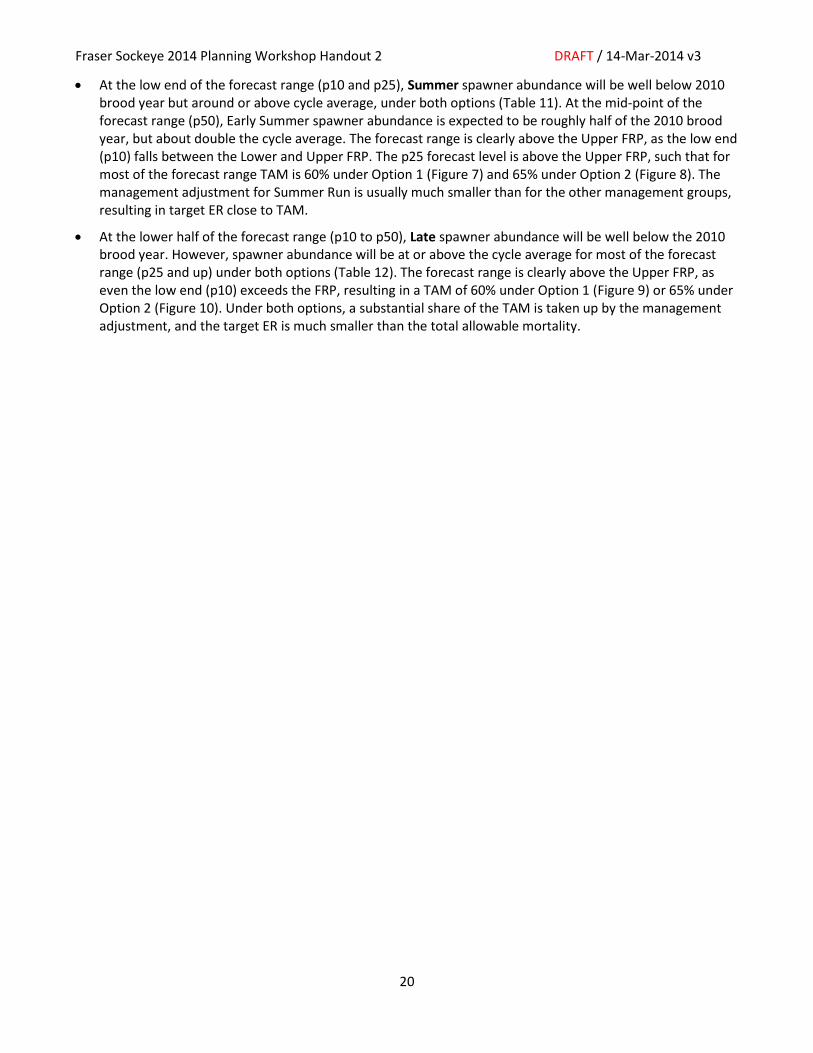
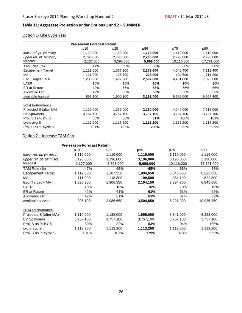
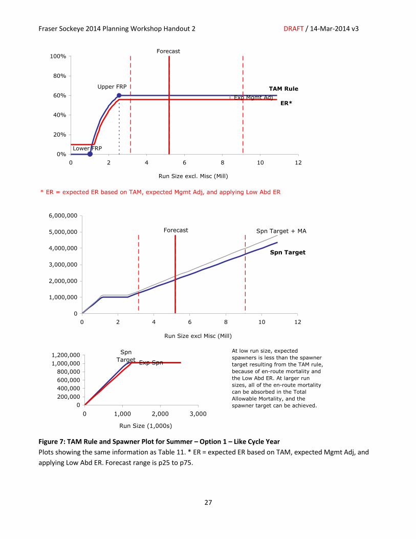
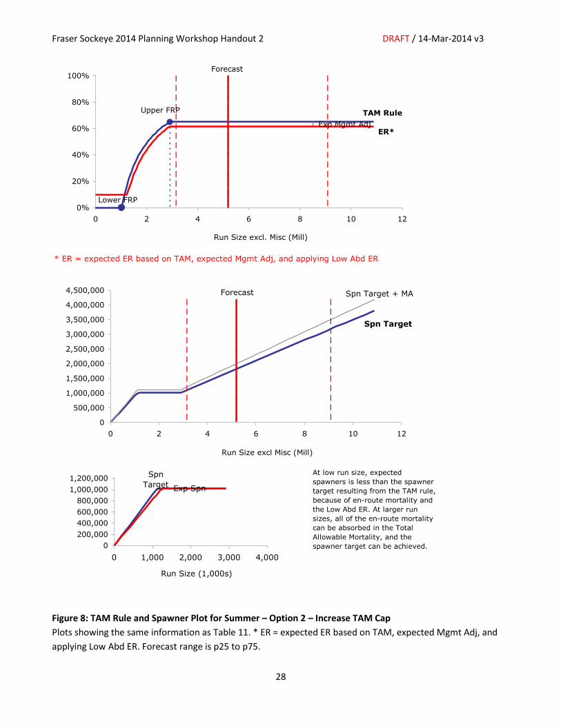
At the low end of the forecast range (p10 and p25), Summer spawner abundance will be well below 2010 brood year but around or above cycle average, under both options (Table 11). At the mid-point of the forecast range (p50), Early Summer spawner abundance is expected to be roughly half of the 2010 brood year, but about double the cycle average. The forecast range is clearly above the Upper FRP, as the low end (p10) falls between the Lower and Upper FRP. The p25 forecast level is above the Upper FRP, such that for most of the forecast range TAM is 60% under Option 1 (Figure 7) and 65% under Option 2 (Figure 8). The management adjustment for Summer Run is usually much smaller than for the other management groups, resulting in target ER close to TAM.
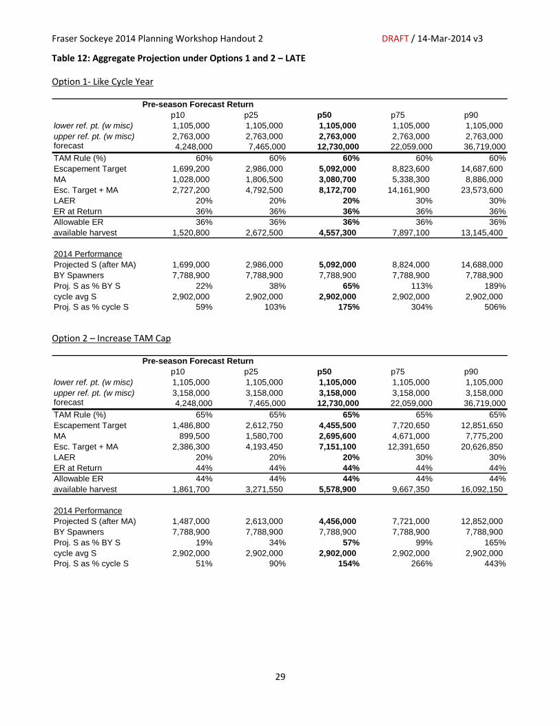
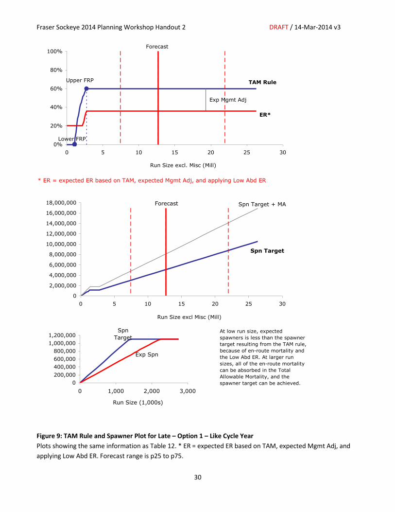
At the lower half of the forecast range (p10 to p50), Late spawner abundance will be well below the 2010 brood year. However, spawner abundance will be at or above the cycle average for most of the forecast range (p25 and up) under both options (Table 12). The forecast range is clearly above the Upper FRP, as even the low end (p10) exceeds the FRP, resulting in a TAM of 60% under Option 1 (Figure 9) or 65% under Option 2 (Figure 10). Under both options, a substantial share of the TAM is taken up by the management adjustment, and the target ER is much smaller than the total allowable mortality.
Fraser Sockeye 2014 Planning Workshop Handout 2 DRAFT / 14-Mar-2014 v3
21
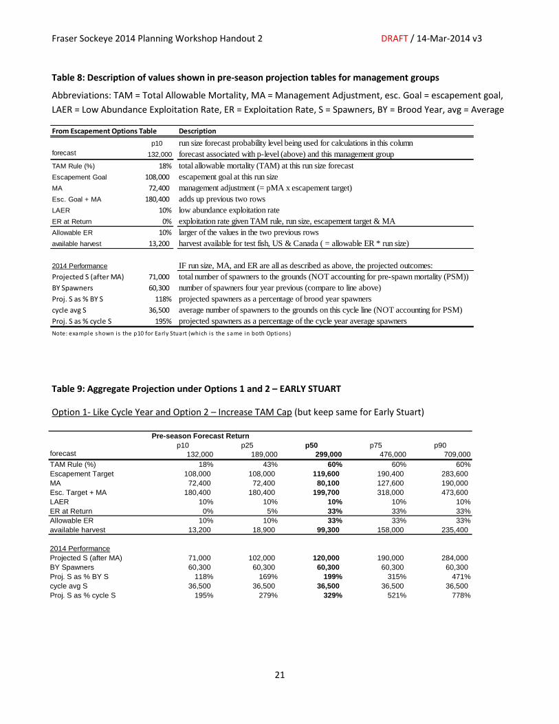
Table 8: Description of values shown in pre-season projection tables for management groups
Abbreviations: TAM = Total Allowable Mortality, MA = Management Adjustment, esc. Goal = escapement goal,
LAER = Low Abundance Exploitation Rate, ER = Exploitation Rate, S = Spawners, BY = Brood Year, avg = Average
Table 9: Aggregate Projection under Options 1 and 2 – EARLY STUART
Option 1- Like Cycle Year and Option 2 – Increase TAM Cap (but keep same for Early Stuart)
Pre-season Forecast Return
p10 p25 p50 p75 p90forecast 132,000 189,000 299,000 476,000 709,000
TAM Rule (%) 18% 43% 60% 60% 60%
Escapement Target 108,000 108,000 119,600 190,400 283,600
MA 72,400 72,400 80,100 127,600 190,000
Esc. Target + MA 180,400 180,400 199,700 318,000 473,600
LAER 10% 10% 10% 10% 10%
ER at Return 0% 5% 33% 33% 33%
Allowable ER 10% 10% 33% 33% 33%
available harvest 13,200 18,900 99,300 158,000 235,400
2014 Performance
Projected S (after MA) 71,000 102,000 120,000 190,000 284,000
BY Spawners 60,300 60,300 60,300 60,300 60,300
Proj. S as % BY S 118% 169% 199% 315% 471%
cycle avg S 36,500 36,500 36,500 36,500 36,500
Proj. S as % cycle S 195% 279% 329% 521% 778%
From Escapement Options Table Description
p10 run size forecast probability level being used for calculations in this columnforecast 132,000 forecast associated with p-level (above) and this management group
TAM Rule (%) 18% total allowable mortality (TAM) at this run size forecast
Escapement Goal 108,000 escapement goal at this run size
MA 72,400 management adjustment (= pMA x escapement target)
Esc. Goal + MA 180,400 adds up previous two rows
LAER 10% low abundance exploitation rate
ER at Return 0% exploitation rate given TAM rule, run size, escapement target & MA
Allowable ER 10% larger of the values in the two previous rows
available harvest 13,200 harvest available for test fish, US & Canada ( = allowable ER * run size)
2014 Performance IF run size, MA, and ER are all as described as above, the projected outcomes:
Projected S (after MA) 71,000 total number of spawners to the grounds (NOT accounting for pre-spawn mortality (PSM))
BY Spawners 60,300 number of spawners four year previous (compare to line above)
Proj. S as % BY S 118% projected spawners as a percentage of brood year spawners
cycle avg S 36,500 average number of spawners to the grounds on this cycle line (NOT accounting for PSM)
Proj. S as % cycle S 195% projected spawners as a percentage of the cycle year average spawners
Note: example shown is the p10 for Early Stuart (which is the same in both Options)
Abbreviations :
TAM - tota l a l lowable mortal i ty
MA - management adjustment
esc. goal - escapement goal
LAER - low abundance expoloi tation rate
ER - exploi tation rate
S - spawners
BY - brood year
avg - average
Fraser Sockeye 2014 Planning Workshop Handout 2 DRAFT / 14-Mar-2014 v3
22
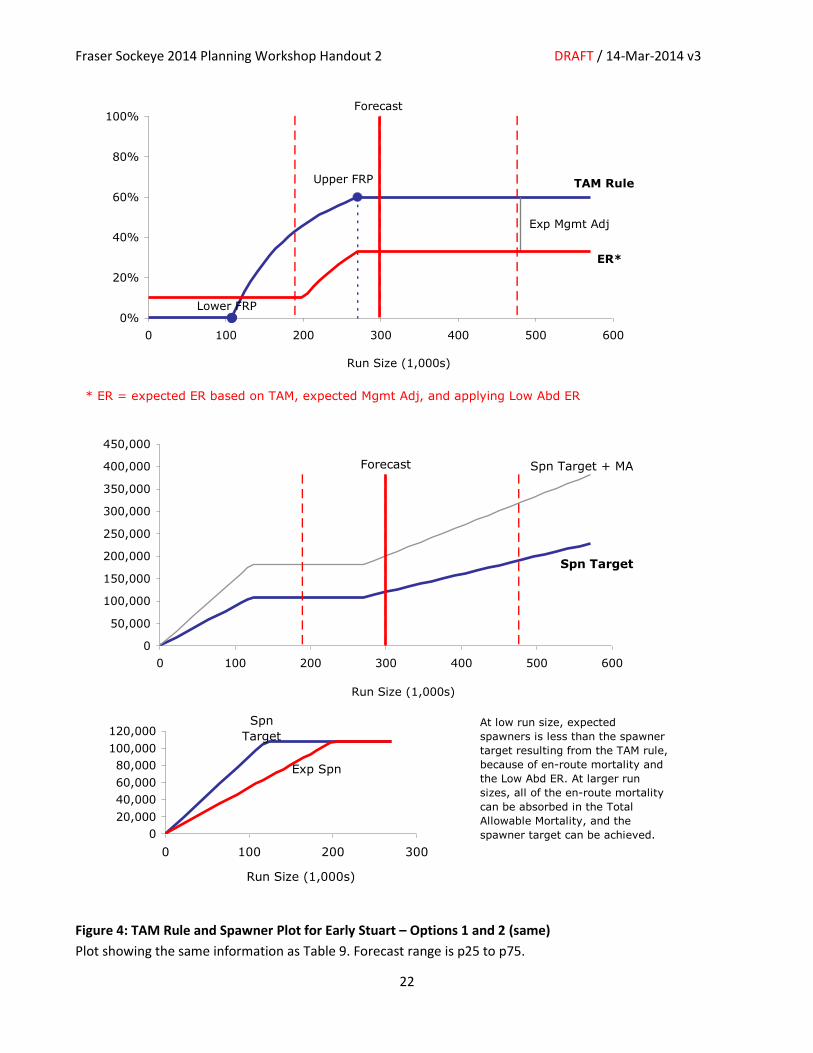
Figure 4: TAM Rule and Spawner Plot for Early Stuart – Options 1 and 2 (same)
Plot showing the same information as Table 9. Forecast range is p25 to p75.
* ER = expected ER based on TAM, expected Mgmt Adj, and applying Low Abd ER
Exp Mgmt Adj
Lower FRP
Upper FRP TAM Rule
ER*
Forecast
0%
20%
40%
60%
80%
100%
0 100 200 300 400 500 600
Run Size (1,000s)
Forecast Spn Target + MA
Spn Target
0
50,000
100,000
150,000
200,000
250,000
300,000
350,000
400,000
450,000
0 100 200 300 400 500 600
Run Size (1,000s)
Exp Spn
Spn
Target
0
20,000
40,000
60,000
80,000
100,000
120,000
0 100 200 300
Run Size (1,000s)
At low run size, expected
spawners is less than the spawner
target resulting from the TAM rule,
because of en-route mortality and
the Low Abd ER. At larger run
sizes, all of the en-route mortality
can be absorbed in the Total
Allowable Mortality, and the
spawner target can be achieved.
Fraser Sockeye 2014 Planning Workshop Handout 2 DRAFT / 14-Mar-2014 v3
23
Table 10: Aggregate Projection under Options 1 and 2 – EARLY SUMMER
Option 1- Like Cycle Year
Option 2 – Increase TAM Cap
Pre-season Forecast Return
p10 p25 p50 p75 p90
lower ref. pt. (w misc) 251,000 245,000 239,000 223,000 218,000
upper ref. pt. (w misc) 628,000 613,000 597,000 557,000 544,000 forecast (incl. misc) 730,000 1,741,000 4,126,000 8,470,000 16,805,000
TAM Rule (%) 60% 60% 60% 60% 60%
Escapement Target 292,000 696,400 1,650,400 3,388,000 6,722,000
MA 125,600 299,500 709,700 1,456,800 2,890,500
Esc. Target + MA 417,600 995,900 2,360,100 4,844,800 9,612,500
LAER 10% 10% 10% 10% 10%
ER at Return 43% 43% 43% 43% 43%
Allowable ER 43% 43% 43% 43% 43%
available harvest 312,400 745,100 1,765,900 3,625,200 7,192,500
2014 Performance
Projected S (after MA) 292,000 696,000 1,650,000 3,388,000 6,722,000
BY Spawners 1,524,700 1,524,700 1,524,700 1,524,700 1,524,700
Proj. S as % BY S 19% 46% 108% 222% 441%
cycle avg S 291,400 291,400 291,400 291,400 291,400
Proj. S as % cycle S 100% 239% 566% 1163% 2307%
Pre-season Forecast Return
p10 p25 p50 p75 p90
lower ref. pt. (w misc) 251,000 245,000 239,000 223,000 218,000
upper ref. pt. (w misc) 718,000 700,000 682,000 636,000 622,000 forecast (incl. misc) 730,000 1,741,000 4,126,000 8,470,000 16,805,000
TAM Rule (%) 65% 65% 65% 65% 65%
Escapement Target 255,500 609,350 1,444,100 2,964,500 5,881,750
MA 109,900 262,000 621,000 1,274,700 2,529,200
Esc. Target + MA 365,400 871,350 2,065,100 4,239,200 8,410,950
LAER 10% 10% 10% 10% 10%
ER at Return 50% 50% 50% 50% 50%
Allowable ER 50% 50% 50% 50% 50%
available harvest 364,600 869,650 2,060,900 4,230,800 8,394,050
2014 Performance
Projected S (after MA) 256,000 609,000 1,444,000 2,964,000 5,882,000
BY Spawners 1,524,700 1,524,700 1,524,700 1,524,700 1,524,700
Proj. S as % BY S 17% 40% 95% 194% 386%
cycle avg S 291,400 291,400 291,400 291,400 291,400
Proj. S as % cycle S 88% 209% 496% 1017% 2019%
Fraser Sockeye 2014 Planning Workshop Handout 2 DRAFT / 14-Mar-2014 v3
24
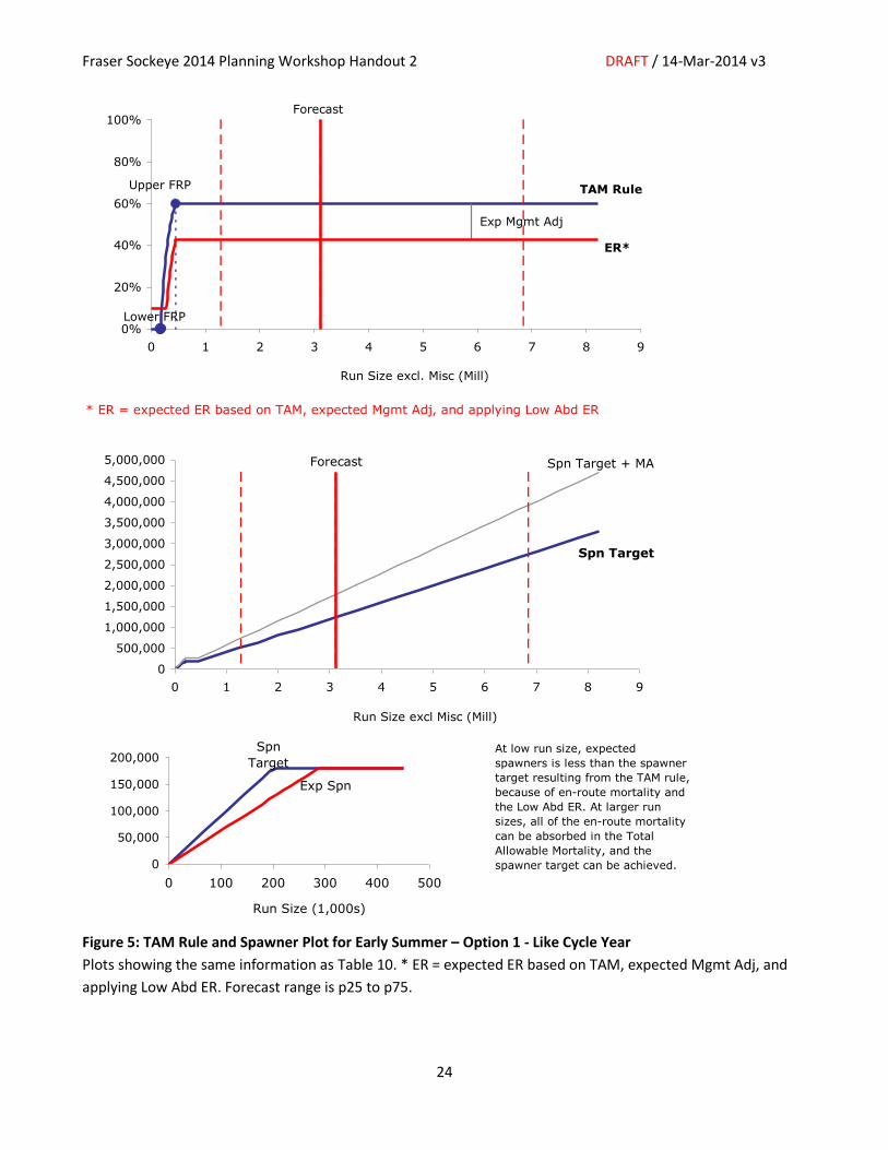
Figure 5: TAM Rule and Spawner Plot for Early Summer – Option 1 - Like Cycle Year
Plots showing the same information as Table 10. * ER = expected ER based on TAM, expected Mgmt Adj, and
applying Low Abd ER. Forecast range is p25 to p75.
* ER = expected ER based on TAM, expected Mgmt Adj, and applying Low Abd ER
Exp Mgmt Adj
Lower FRP
Upper FRP TAM Rule
ER*
Forecast
0%
20%
40%
60%
80%
100%
0 1 2 3 4 5 6 7 8 9
Run Size excl. Misc (Mill)
Forecast Spn Target + MA
Spn Target
0
500,000
1,000,000
1,500,000
2,000,000
2,500,000
3,000,000
3,500,000
4,000,000
4,500,000
5,000,000
0 1 2 3 4 5 6 7 8 9
Run Size excl Misc (Mill)
Exp Spn
Spn
Target
0
50,000
100,000
150,000
200,000
0 100 200 300 400 500
Run Size (1,000s)
At low run size, expected
spawners is less than the spawner
target resulting from the TAM rule,
because of en-route mortality and
the Low Abd ER. At larger run
sizes, all of the en-route mortality
can be absorbed in the Total
Allowable Mortality, and the
spawner target can be achieved.
Fraser Sockeye 2014 Planning Workshop Handout 2 DRAFT / 14-Mar-2014 v3
25
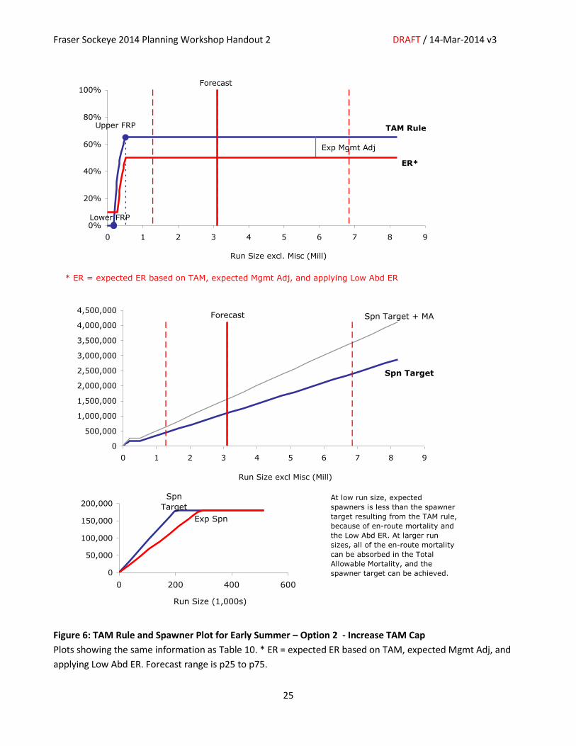
Figure 6: TAM Rule and Spawner Plot for Early Summer – Option 2 - Increase TAM Cap
Plots showing the same information as Table 10. * ER = expected ER based on TAM, expected Mgmt Adj, and
applying Low Abd ER. Forecast range is p25 to p75.
* ER = expected ER based on TAM, expected Mgmt Adj, and applying Low Abd ER
Exp Mgmt Adj
Lower FRP
Upper FRP TAM Rule
ER*
Forecast
0%
20%
40%
60%
80%
100%
0 1 2 3 4 5 6 7 8 9
Run Size excl. Misc (Mill)
Forecast Spn Target + MA
Spn Target
0
500,000
1,000,000
1,500,000
2,000,000
2,500,000
3,000,000
3,500,000
4,000,000
4,500,000
0 1 2 3 4 5 6 7 8 9
Run Size excl Misc (Mill)
Exp Spn
Spn
Target
0
50,000
100,000
150,000
200,000
0 200 400 600
Run Size (1,000s)
At low run size, expected
spawners is less than the spawner
target resulting from the TAM rule,
because of en-route mortality and
the Low Abd ER. At larger run
sizes, all of the en-route mortality
can be absorbed in the Total
Allowable Mortality, and the
spawner target can be achieved.
Fraser Sockeye 2014 Planning Workshop Handout 2 DRAFT / 14-Mar-2014 v3
26
Table 11: Aggregate Projection under Options 1 and 2 – SUMMER
Option 1- Like Cycle Year
Option 2 – Increase TAM Cap
Pre-season Forecast Return
p10 p25 p50 p75 p90
lower ref. pt. (w misc) 1,119,000 1,119,000 1,119,000 1,119,000 1,119,000
upper ref. pt. (w misc) 2,796,000 2,796,000 2,796,000 2,796,000 2,796,000 forecast 2,127,000 3,393,000 5,699,000 10,116,000 17,781,000
TAM Rule (%) 47% 60% 60% 60% 60%
Escapement Target 1,119,000 1,357,200 2,279,600 4,046,400 7,112,400
MA 111,900 135,700 228,000 404,600 711,200
Esc. Target + MA 1,230,900 1,492,900 2,507,600 4,451,000 7,823,600
LAER 10% 10% 10% 10% 10%
ER at Return 42% 56% 56% 56% 56%
Allowable ER 42% 56% 56% 56% 56%
available harvest 896,100 1,900,100 3,191,400 5,665,000 9,957,400
2014 Performance
Projected S (after MA) 1,119,000 1,357,000 2,280,000 4,046,000 7,112,000
BY Spawners 3,757,100 3,757,100 3,757,100 3,757,100 3,757,100
Proj. S as % BY S 30% 36% 61% 108% 189%
cycle avg S 1,113,200 1,113,200 1,113,200 1,113,200 1,113,200
Proj. S as % cycle S 101% 122% 205% 363% 639%
Pre-season Forecast Return
p10 p25 p50 p75 p90
lower ref. pt. (w misc) 1,119,000 1,119,000 1,119,000 1,119,000 1,119,000
upper ref. pt. (w misc) 3,196,000 3,196,000 3,196,000 3,196,000 3,196,000 forecast 2,127,000 3,393,000 5,699,000 10,116,000 17,781,000
TAM Rule (%) 47% 65% 65% 65% 65%
Escapement Target 1,119,000 1,187,550 1,994,650 3,540,600 6,223,350
MA 111,900 118,800 199,500 354,100 622,300
Esc. Target + MA 1,230,900 1,306,350 2,194,150 3,894,700 6,845,650
LAER 10% 10% 10% 10% 10%
ER at Return 42% 61% 61% 61% 62%
Allowable ER 42% 61% 61% 61% 62%
available harvest 896,100 2,086,650 3,504,850 6,221,300 10,935,350
2014 Performance
Projected S (after MA) 1,119,000 1,188,000 1,995,000 3,541,000 6,223,000
BY Spawners 3,757,100 3,757,100 3,757,100 3,757,100 3,757,100
Proj. S as % BY S 30% 32% 53% 94% 166%
cycle avg S 1,113,200 1,113,200 1,113,200 1,113,200 1,113,200
Proj. S as % cycle S 101% 107% 179% 318% 559%
Fraser Sockeye 2014 Planning Workshop Handout 2 DRAFT / 14-Mar-2014 v3
27
Figure 7: TAM Rule and Spawner Plot for Summer – Option 1 – Like Cycle Year
Plots showing the same information as Table 11. * ER = expected ER based on TAM, expected Mgmt Adj, and
applying Low Abd ER. Forecast range is p25 to p75.
* ER = expected ER based on TAM, expected Mgmt Adj, and applying Low Abd ER
Exp Mgmt Adj
Lower FRP
Upper FRP TAM Rule
ER*
Forecast
0%
20%
40%
60%
80%
100%
0 2 4 6 8 10 12
Run Size excl. Misc (Mill)
Forecast Spn Target + MA
Spn Target
0
1,000,000
2,000,000
3,000,000
4,000,000
5,000,000
6,000,000
0 2 4 6 8 10 12
Run Size excl Misc (Mill)
Exp Spn
Spn
Target
0
200,000
400,000
600,000
800,000
1,000,000
1,200,000
0 1,000 2,000 3,000
Run Size (1,000s)
At low run size, expected
spawners is less than the spawner
target resulting from the TAM rule,
because of en-route mortality and
the Low Abd ER. At larger run
sizes, all of the en-route mortality
can be absorbed in the Total
Allowable Mortality, and the
spawner target can be achieved.
Fraser Sockeye 2014 Planning Workshop Handout 2 DRAFT / 14-Mar-2014 v3
28
Figure 8: TAM Rule and Spawner Plot for Summer – Option 2 – Increase TAM Cap
Plots showing the same information as Table 11. * ER = expected ER based on TAM, expected Mgmt Adj, and
applying Low Abd ER. Forecast range is p25 to p75.
* ER = expected ER based on TAM, expected Mgmt Adj, and applying Low Abd ER
Exp Mgmt Adj
Lower FRP
Upper FRP TAM Rule
ER*
Forecast
0%
20%
40%
60%
80%
100%
0 2 4 6 8 10 12
Run Size excl. Misc (Mill)
Forecast Spn Target + MA
Spn Target
0
500,000
1,000,000
1,500,000
2,000,000
2,500,000
3,000,000
3,500,000
4,000,000
4,500,000
0 2 4 6 8 10 12
Run Size excl Misc (Mill)
Exp Spn
Spn
Target
0
200,000
400,000
600,000
800,000
1,000,000
1,200,000
0 1,000 2,000 3,000 4,000
Run Size (1,000s)
At low run size, expected
spawners is less than the spawner
target resulting from the TAM rule,
because of en-route mortality and
the Low Abd ER. At larger run
sizes, all of the en-route mortality
can be absorbed in the Total
Allowable Mortality, and the
spawner target can be achieved.
Fraser Sockeye 2014 Planning Workshop Handout 2 DRAFT / 14-Mar-2014 v3
29
Table 12: Aggregate Projection under Options 1 and 2 – LATE
Option 1- Like Cycle Year
Option 2 – Increase TAM Cap
Pre-season Forecast Return
p10 p25 p50 p75 p90
lower ref. pt. (w misc) 1,105,000 1,105,000 1,105,000 1,105,000 1,105,000
upper ref. pt. (w misc) 2,763,000 2,763,000 2,763,000 2,763,000 2,763,000 forecast 4,248,000 7,465,000 12,730,000 22,059,000 36,719,000
TAM Rule (%) 60% 60% 60% 60% 60%
Escapement Target 1,699,200 2,986,000 5,092,000 8,823,600 14,687,600
MA 1,028,000 1,806,500 3,080,700 5,338,300 8,886,000
Esc. Target + MA 2,727,200 4,792,500 8,172,700 14,161,900 23,573,600
LAER 20% 20% 20% 30% 30%
ER at Return 36% 36% 36% 36% 36%
Allowable ER 36% 36% 36% 36% 36%
available harvest 1,520,800 2,672,500 4,557,300 7,897,100 13,145,400
2014 Performance
Projected S (after MA) 1,699,000 2,986,000 5,092,000 8,824,000 14,688,000
BY Spawners 7,788,900 7,788,900 7,788,900 7,788,900 7,788,900
Proj. S as % BY S 22% 38% 65% 113% 189%
cycle avg S 2,902,000 2,902,000 2,902,000 2,902,000 2,902,000
Proj. S as % cycle S 59% 103% 175% 304% 506%
Pre-season Forecast Return
p10 p25 p50 p75 p90
lower ref. pt. (w misc) 1,105,000 1,105,000 1,105,000 1,105,000 1,105,000
upper ref. pt. (w misc) 3,158,000 3,158,000 3,158,000 3,158,000 3,158,000 forecast 4,248,000 7,465,000 12,730,000 22,059,000 36,719,000
TAM Rule (%) 65% 65% 65% 65% 65%
Escapement Target 1,486,800 2,612,750 4,455,500 7,720,650 12,851,650
MA 899,500 1,580,700 2,695,600 4,671,000 7,775,200
Esc. Target + MA 2,386,300 4,193,450 7,151,100 12,391,650 20,626,850
LAER 20% 20% 20% 30% 30%
ER at Return 44% 44% 44% 44% 44%
Allowable ER 44% 44% 44% 44% 44%
available harvest 1,861,700 3,271,550 5,578,900 9,667,350 16,092,150
2014 Performance
Projected S (after MA) 1,487,000 2,613,000 4,456,000 7,721,000 12,852,000
BY Spawners 7,788,900 7,788,900 7,788,900 7,788,900 7,788,900
Proj. S as % BY S 19% 34% 57% 99% 165%
cycle avg S 2,902,000 2,902,000 2,902,000 2,902,000 2,902,000
Proj. S as % cycle S 51% 90% 154% 266% 443%
Fraser Sockeye 2014 Planning Workshop Handout 2 DRAFT / 14-Mar-2014 v3
30
Figure 9: TAM Rule and Spawner Plot for Late – Option 1 – Like Cycle Year
Plots showing the same information as Table 12. * ER = expected ER based on TAM, expected Mgmt Adj, and
applying Low Abd ER. Forecast range is p25 to p75.
* ER = expected ER based on TAM, expected Mgmt Adj, and applying Low Abd ER
Exp Mgmt Adj
Lower FRP
Upper FRP TAM Rule
ER*
Forecast
0%
20%
40%
60%
80%
100%
0 5 10 15 20 25 30
Run Size excl. Misc (Mill)
Forecast Spn Target + MA
Spn Target
0
2,000,000
4,000,000
6,000,000
8,000,000
10,000,000
12,000,000
14,000,000
16,000,000
18,000,000
0 5 10 15 20 25 30
Run Size excl Misc (Mill)
Exp Spn
Spn
Target
0
200,000
400,000
600,000
800,000
1,000,000
1,200,000
0 1,000 2,000 3,000
Run Size (1,000s)
At low run size, expected
spawners is less than the spawner
target resulting from the TAM rule,
because of en-route mortality and
the Low Abd ER. At larger run
sizes, all of the en-route mortality
can be absorbed in the Total
Allowable Mortality, and the
spawner target can be achieved.
Fraser Sockeye 2014 Planning Workshop Handout 2 DRAFT / 14-Mar-2014 v3
31
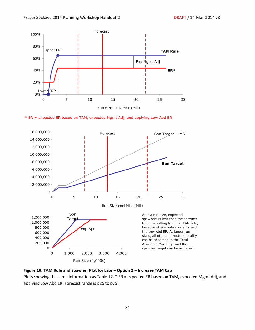
Figure 10: TAM Rule and Spawner Plot for Late – Option 2 – Increase TAM Cap
Plots showing the same information as Table 12. * ER = expected ER based on TAM, expected Mgmt Adj, and
applying Low Abd ER. Forecast range is p25 to p75.
* ER = expected ER based on TAM, expected Mgmt Adj, and applying Low Abd ER
Exp Mgmt Adj
Lower FRP
Upper FRP TAM Rule
ER*
Forecast
0%
20%
40%
60%
80%
100%
0 5 10 15 20 25 30
Run Size excl. Misc (Mill)
Forecast Spn Target + MA
Spn Target
0
2,000,000
4,000,000
6,000,000
8,000,000
10,000,000
12,000,000
14,000,000
16,000,000
0 5 10 15 20 25 30
Run Size excl Misc (Mill)
Exp Spn
Spn
Target
0
200,000
400,000
600,000
800,000
1,000,000
1,200,000
0 1,000 2,000 3,000 4,000
Run Size (1,000s)
At low run size, expected
spawners is less than the spawner
target resulting from the TAM rule,
because of en-route mortality and
the Low Abd ER. At larger run
sizes, all of the en-route mortality
can be absorbed in the Total
Allowable Mortality, and the
spawner target can be achieved.
Fraser Sockeye 2014 Planning Workshop Handout 2 DRAFT / 14-Mar-2014 v3
32
Comparing Expected Outcomes for Options 1 and 2 – By Stock
Table 13 shows the projected spawner abundance for each forecasted stock over the range of forecast
probability levels for each option and compares it long-term average spawners for that stock. Stock-specific
projections are calculated from the “projected S (after MA)” in Table 9 to Table 12, which is distributed to the
component stocks based on the proportion each stock contributes to the forecast at each p-level. Note that
this makes the additional assumption that the exploitation rate will be distributed evenly within a management
group.)
Table 13 compares projected spawner abundances to long-term mean and the cycle average. Table 14
compares projected spawner abundances to the high end of observed abundances. Figure 11 and Figure 12
show how projected spawner abundances for the 2 options compare to the observed time series pattern (line
plot) and to the observed distribution (histogram).
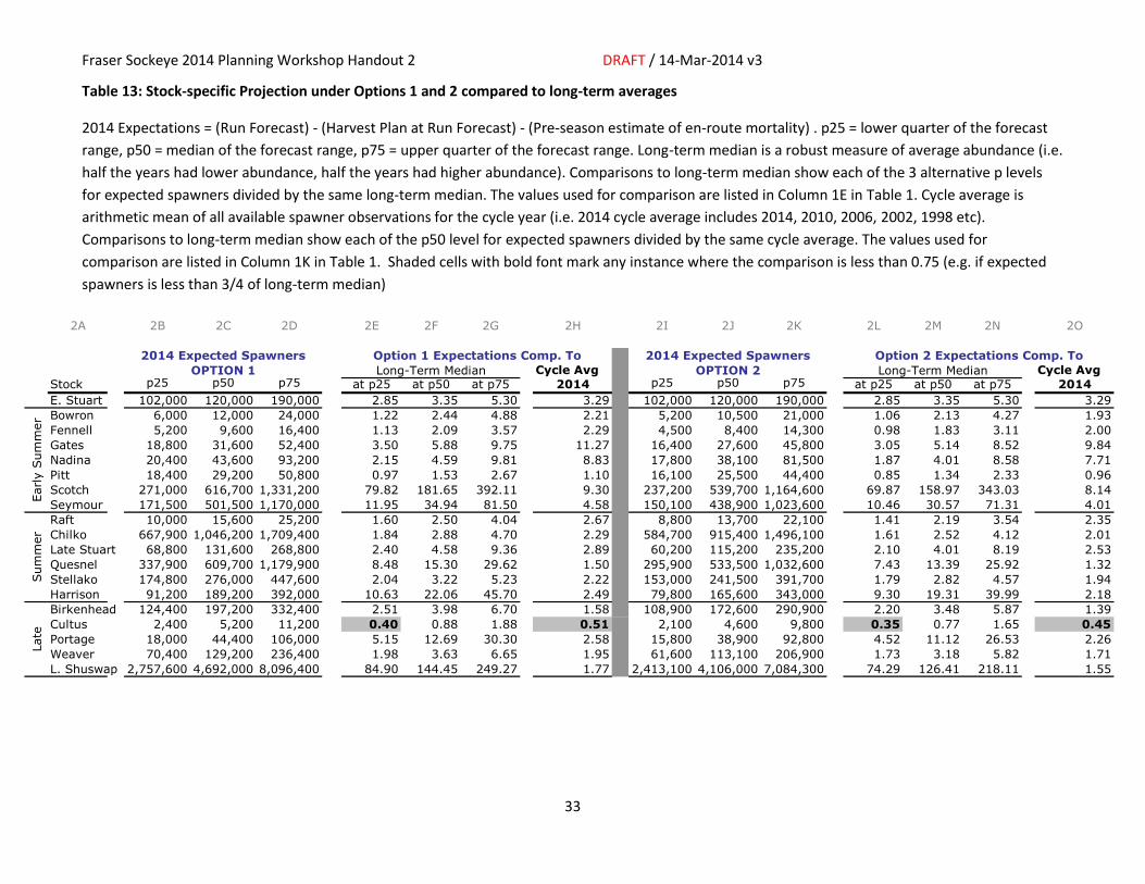
Key points to note in Table 13 are:
For 18 of the 19 stocks, the projected spawners under both options are near or above both the long-term median and the 2014 cycle average. The exception is Cultus (shaded in grey).
For several of the stocks, the projected spawner abundance under both options is much larger than the long-term median (up to almost 400 times larger!) (Col 2E to 2G). These stocks are: Scotch, Seymour, Quesnel, Harrison, and Late Shuswap. Note however, that the median by definition gives lower numbers than the arithmetic mean for data sets with a few large outliers, such as the very large spawner abundances in the dominant cycle year. By contrast, the comparisons to cycle average indicate a less drastic difference. The same stocks have projected spawner abundances about 5-10 times larger than the cycle average.
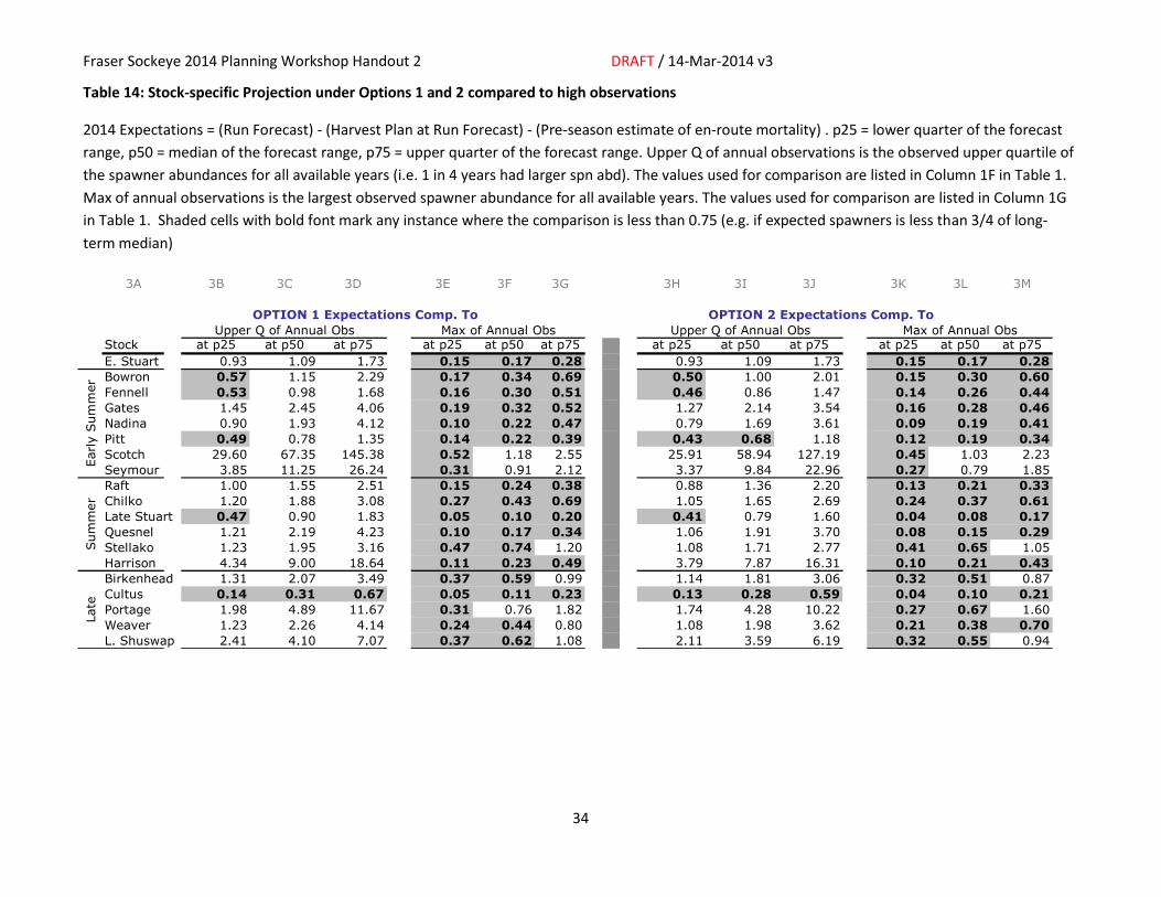
Key points to note in Table 14 are:
At the upper half of the forecast range (p50 and up), the projected spawners are above the upper quarter of the observed range for 18 of the 19 stocks under Option 1 (Col 3C and 3D). The exception is Cultus. Under Option 2, projected spawners for Pitt also fall below the upper quartile at the p50 forecast level (Col 3I)
Projected spawners for 12 of the 19 stocks fall below the highest observed spawner abundance under both options (Col 3E to 3G and 3K to 3M). The exceptions are Scotch, Seymour, Stellako, Birkenhead, Portage, Weaver, Late Shuswap. For these stocks, projected spawner abundance is roughly 1.5 to 2 times larger the largest previous observed.
Figure 11 and Figure 12 show the same information as the summary tables throughout this document, just in
condensed form without the details.
Fraser Sockeye 2014 Planning Workshop Handout 2 DRAFT / 14-Mar-2014 v3
33
Table 13: Stock-specific Projection under Options 1 and 2 compared to long-term averages
2014 Expectations = (Run Forecast) - (Harvest Plan at Run Forecast) - (Pre-season estimate of en-route mortality) . p25 = lower quarter of the forecast
range, p50 = median of the forecast range, p75 = upper quarter of the forecast range. Long-term median is a robust measure of average abundance (i.e.
half the years had lower abundance, half the years had higher abundance). Comparisons to long-term median show each of the 3 alternative p levels
for expected spawners divided by the same long-term median. The values used for comparison are listed in Column 1E in Table 1. Cycle average is
arithmetic mean of all available spawner observations for the cycle year (i.e. 2014 cycle average includes 2014, 2010, 2006, 2002, 1998 etc).
Comparisons to long-term median show each of the p50 level for expected spawners divided by the same cycle average. The values used for
comparison are listed in Column 1K in Table 1. Shaded cells with bold font mark any instance where the comparison is less than 0.75 (e.g. if expected
spawners is less than 3/4 of long-term median)
2A 2B 2C 2D 2E 2F 2G 2H 2I 2J 2K 2L 2M 2N 2O
Cycle Avg Cycle Avg
Stock p25 p50 p75 at p25 at p50 at p75 2014 p25 p50 p75 at p25 at p50 at p75 2014
E. Stuart 102,000 120,000 190,000 2.85 3.35 5.30 3.29 102,000 120,000 190,000 2.85 3.35 5.30 3.29
Bowron 6,000 12,000 24,000 1.22 2.44 4.88 2.21 5,200 10,500 21,000 1.06 2.13 4.27 1.93
Fennell 5,200 9,600 16,400 1.13 2.09 3.57 2.29 4,500 8,400 14,300 0.98 1.83 3.11 2.00
Gates 18,800 31,600 52,400 3.50 5.88 9.75 11.27 16,400 27,600 45,800 3.05 5.14 8.52 9.84
Nadina 20,400 43,600 93,200 2.15 4.59 9.81 8.83 17,800 38,100 81,500 1.87 4.01 8.58 7.71
Pitt 18,400 29,200 50,800 0.97 1.53 2.67 1.10 16,100 25,500 44,400 0.85 1.34 2.33 0.96
Scotch 271,000 616,700 1,331,200 79.82 181.65 392.11 9.30 237,200 539,700 1,164,600 69.87 158.97 343.03 8.14
Seymour 171,500 501,500 1,170,000 11.95 34.94 81.50 4.58 150,100 438,900 1,023,600 10.46 30.57 71.31 4.01
Raft 10,000 15,600 25,200 1.60 2.50 4.04 2.67 8,800 13,700 22,100 1.41 2.19 3.54 2.35
Chilko 667,900 1,046,200 1,709,400 1.84 2.88 4.70 2.29 584,700 915,400 1,496,100 1.61 2.52 4.12 2.01
Late Stuart 68,800 131,600 268,800 2.40 4.58 9.36 2.89 60,200 115,200 235,200 2.10 4.01 8.19 2.53
Quesnel 337,900 609,700 1,179,900 8.48 15.30 29.62 1.50 295,900 533,500 1,032,600 7.43 13.39 25.92 1.32
Stellako 174,800 276,000 447,600 2.04 3.22 5.23 2.22 153,000 241,500 391,700 1.79 2.82 4.57 1.94
Harrison 91,200 189,200 392,000 10.63 22.06 45.70 2.49 79,800 165,600 343,000 9.30 19.31 39.99 2.18
Birkenhead 124,400 197,200 332,400 2.51 3.98 6.70 1.58 108,900 172,600 290,900 2.20 3.48 5.87 1.39
Cultus 2,400 5,200 11,200 0.40 0.88 1.88 0.51 2,100 4,600 9,800 0.35 0.77 1.65 0.45
Portage 18,000 44,400 106,000 5.15 12.69 30.30 2.58 15,800 38,900 92,800 4.52 11.12 26.53 2.26
Weaver 70,400 129,200 236,400 1.98 3.63 6.65 1.95 61,600 113,100 206,900 1.73 3.18 5.82 1.71
L. Shuswap 2,757,600 4,692,000 8,096,400 84.90 144.45 249.27 1.77 2,413,100 4,106,000 7,084,300 74.29 126.41 218.11 1.55
Sum
mer
Late
Early S
um
mer
Option 2 Expectations Comp. To2014 Expected Spawners
OPTION 2 Long-Term Median
Option 1 Expectations Comp. To
OPTION 1 Long-Term Median
2014 Expected Spawners
Fraser Sockeye 2014 Planning Workshop Handout 2 DRAFT / 14-Mar-2014 v3
34
Table 14: Stock-specific Projection under Options 1 and 2 compared to high observations
2014 Expectations = (Run Forecast) - (Harvest Plan at Run Forecast) - (Pre-season estimate of en-route mortality) . p25 = lower quarter of the forecast
range, p50 = median of the forecast range, p75 = upper quarter of the forecast range. Upper Q of annual observations is the observed upper quartile of
the spawner abundances for all available years (i.e. 1 in 4 years had larger spn abd). The values used for comparison are listed in Column 1F in Table 1.
Max of annual observations is the largest observed spawner abundance for all available years. The values used for comparison are listed in Column 1G
in Table 1. Shaded cells with bold font mark any instance where the comparison is less than 0.75 (e.g. if expected spawners is less than 3/4 of long-
term median)
3A 3B 3C 3D 3E 3F 3G 3H 3I 3J 3K 3L 3M
OPTION 1 Expectations Comp. To OPTION 2 Expectations Comp. To
Stock at p25 at p50 at p75 at p25 at p50 at p75 at p25 at p50 at p75 at p25 at p50 at p75
E. Stuart 0.93 1.09 1.73 0.15 0.17 0.28 0.93 1.09 1.73 0.15 0.17 0.28
Bowron 0.57 1.15 2.29 0.17 0.34 0.69 0.50 1.00 2.01 0.15 0.30 0.60
Fennell 0.53 0.98 1.68 0.16 0.30 0.51 0.46 0.86 1.47 0.14 0.26 0.44
Gates 1.45 2.45 4.06 0.19 0.32 0.52 1.27 2.14 3.54 0.16 0.28 0.46
Nadina 0.90 1.93 4.12 0.10 0.22 0.47 0.79 1.69 3.61 0.09 0.19 0.41
Pitt 0.49 0.78 1.35 0.14 0.22 0.39 0.43 0.68 1.18 0.12 0.19 0.34
Scotch 29.60 67.35 145.38 0.52 1.18 2.55 25.91 58.94 127.19 0.45 1.03 2.23
Seymour 3.85 11.25 26.24 0.31 0.91 2.12 3.37 9.84 22.96 0.27 0.79 1.85
Raft 1.00 1.55 2.51 0.15 0.24 0.38 0.88 1.36 2.20 0.13 0.21 0.33
Chilko 1.20 1.88 3.08 0.27 0.43 0.69 1.05 1.65 2.69 0.24 0.37 0.61
Late Stuart 0.47 0.90 1.83 0.05 0.10 0.20 0.41 0.79 1.60 0.04 0.08 0.17
Quesnel 1.21 2.19 4.23 0.10 0.17 0.34 1.06 1.91 3.70 0.08 0.15 0.29
Stellako 1.23 1.95 3.16 0.47 0.74 1.20 1.08 1.71 2.77 0.41 0.65 1.05
Harrison 4.34 9.00 18.64 0.11 0.23 0.49 3.79 7.87 16.31 0.10 0.21 0.43
Birkenhead 1.31 2.07 3.49 0.37 0.59 0.99 1.14 1.81 3.06 0.32 0.51 0.87
Cultus 0.14 0.31 0.67 0.05 0.11 0.23 0.13 0.28 0.59 0.04 0.10 0.21
Portage 1.98 4.89 11.67 0.31 0.76 1.82 1.74 4.28 10.22 0.27 0.67 1.60
Weaver 1.23 2.26 4.14 0.24 0.44 0.80 1.08 1.98 3.62 0.21 0.38 0.70
L. Shuswap 2.41 4.10 7.07 0.37 0.62 1.08 2.11 3.59 6.19 0.32 0.55 0.94
Early S
um
mer
Sum
mer
Late
Upper Q of Annual Obs Upper Q of Annual Obs Max of Annual ObsMax of Annual Obs
Fraser Sockeye 2014 Planning Workshop Handout 2 DRAFT / 14-Mar-2014 v3
35
Early Stuart
Early Summer
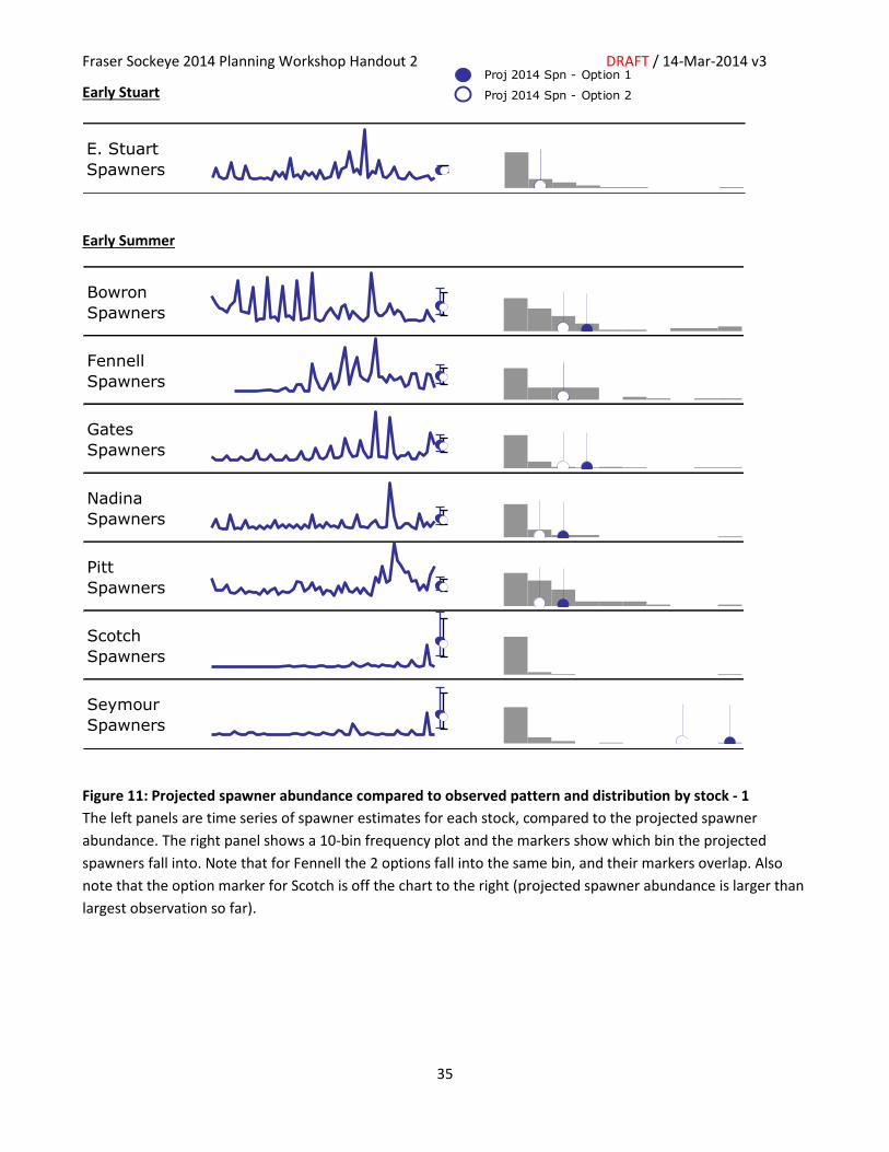
Figure 11: Projected spawner abundance compared to observed pattern and distribution by stock - 1
The left panels are time series of spawner estimates for each stock, compared to the projected spawner
abundance. The right panel shows a 10-bin frequency plot and the markers show which bin the projected
spawners fall into. Note that for Fennell the 2 options fall into the same bin, and their markers overlap. Also
note that the option marker for Scotch is off the chart to the right (projected spawner abundance is larger than
largest observation so far).
Bowron
Spawners
Fennell
Spawners
Gates
Spawners
Nadina
Spawners
Pitt
Spawners
Scotch
Spawners
Seymour
Spawners
Proj 2014 Spn - Option 1
Proj 2014 Spn - Option 2
E. Stuart
Spawners
Fraser Sockeye 2014 Planning Workshop Handout 2 DRAFT / 14-Mar-2014 v3
36
Summer
Late
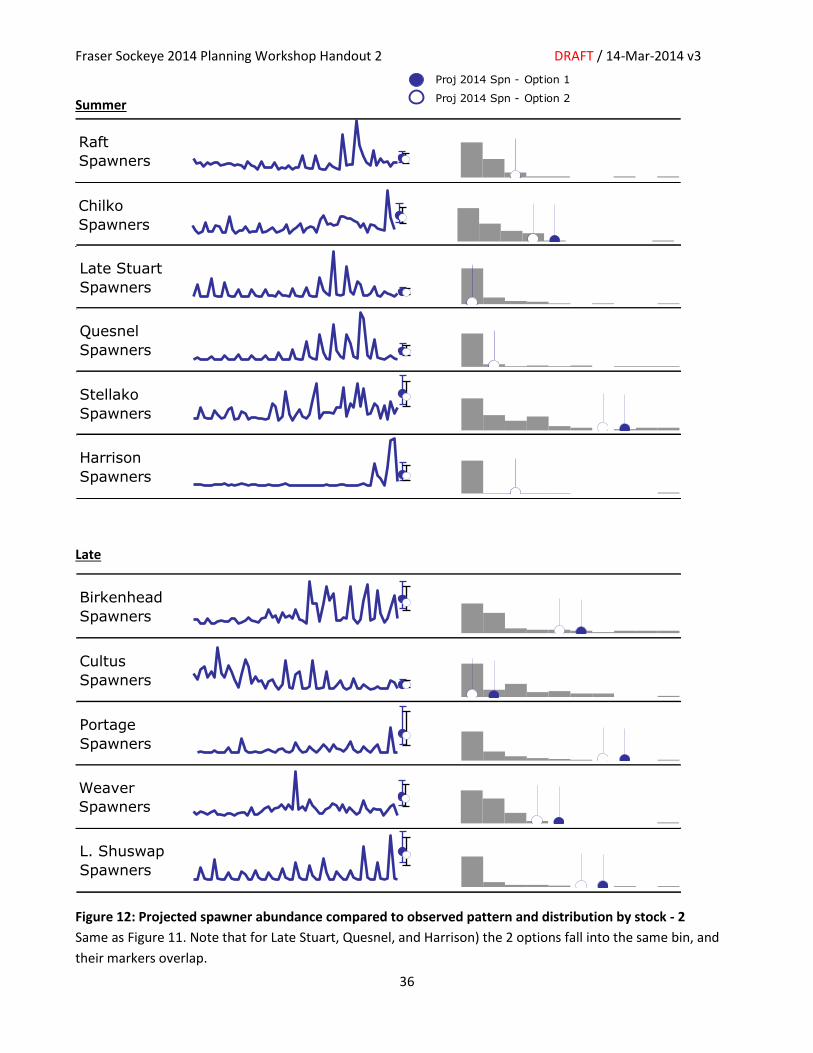
Figure 12: Projected spawner abundance compared to observed pattern and distribution by stock - 2
Same as Figure 11. Note that for Late Stuart, Quesnel, and Harrison) the 2 options fall into the same bin, and
their markers overlap.
Chilko
Spawners
Late Stuart
Spawners
Quesnel
Spawners
Stellako
Spawners
Harrison
Spawners
Birkenhead
Spawners
Cultus
Spawners
Portage
Spawners
L. Shuswap
Spawners
Raft
Spawners
Weaver
Spawners
Proj 2014 Spn - Option 1
Proj 2014 Spn - Option 2
Fraser Sockeye 2014 Planning Workshop Handout 2 DRAFT / 14-Mar-2014 v3
37
4. Additional Considerations
The two options presented in Chapter 3 describe the general harvest plan for Fraser Sockeye. However, the
actual implementation will take additional considerations into account:
Potential fisheries to harvest Excess Salmon to Spawning Requirements (ESSR)
Potential modifications to the Management Adjustment (MA) for very large run sizes
Recovery Objectives for Cultus Lake Sockeye
The rest of this chapter discusses the basis for each of these considerations and explains how they are being
taken into account in the pre-season planning process.
Potential fisheries to harvest Excess Salmon to Spawning Requirements (ESSR)
Based on the 2014 return forecasts, if survival has been average to above-average and returns fall at the mid-to-higher forecast probability levels, returns will fall above cycle averages for a number of stocks, and may potentially be the largest on record. To prepare for the possibility that returns could fall at the higher end of the forecast distribution, opportunities for additional harvest on abundant stocks are being considered.
At the aggregate run-timing-group level, any decision to increase harvest levels should consider the individual survivals of each of the component stocks, as well as en-route mortality (assessed as management adjustments: MA’s in-season). As a result, option 2 with increased TAM cap has been included, but this increases TAM by only by 5%.
At the stock-specific level, additional opportunities may be considered. The steps towards planning such a fishery should consider:
Look at projected spawners after aggregate harvest and MA;
Consider an ESSR if projected spawner abundance is much larger the estimated capacity for the system. (i.e. capacity estimate);
The ceiling level for an ESSR harvest could be = x% of projected spawners in excess to above the capacity estimate, where x may be 50% (e.g. at very large run sizes, drop half the management adjustment)
The following information would assist in making a decision:
Knowledge of what the limiting factor is (spawning habitat or rearing lake?);
Capacity estimate for that limiting factor if available, including estimates of inter-annual variability and uncertainty;
A potential buffer above capacity estimate to account for inter-annual variability and uncertainty;
In practice, however, we do not have firm capacity estimates and for many stocks we do not have any estimates. Instead, various alternatives such as the cycle average escapement, largest observed escapement, etc. could be considered. Table 15 summarizes available lake capacity data. Note that for some rearing lakes the sample size (N) is not good (in some cases only 1). Key points to remember are:
spawning capacity might be limiting over rearing lake capacity, but we do not have spawning capacity estimates
there are multiple stocks using rearing lakes that contribute to lake capacity; so can't look at one stock in isolation of others in these cases
shift in lake-rearing capacity in recent years for particularly Chilko and Shuswap for different reasons;
Fraser Sockeye 2014 Planning Workshop Handout 2 DRAFT / 14-Mar-2014 v3
38
Specific considerations related capacity 2014:
Late Shuswap: exceptional escapements in 2010; key issue is we only have lake rearing capacity estimates for this system, and in recent years these values have changed (increased). So using historical Smax estimates for Fraser Sockeye for this system is problematic if you want to estimate the variation in these estimates, as this system is now in a new period of production. In addition, most fry rear in the main arm of Shuswap Lake and other stocks (early-timed Shuswap stocks) also use the rearing lake and will contribute lake-rearing fry densities.
Early Shuswap: exceptional escapements in 2010; likely limited by spawning capacity rather than lake rearing capacity; we do not have estimates of spawning capacity for this system (the estimates in the FRAP report should not be used, as in the 2011 Fraser Sockeye Stock Status Canadian Science Advisory Secretariat process the Salmon Sub-Committee consensus was to not use them given the lack of documentation of methods and peer review of these values. Again, most fry rear in the main arm of Shuswap Lake and these stocks will contribute to the lake rearing fry densities.
Chilko: exceptional escapements in 2010, however, given low freshwater survival, total smolt outmigration was above average but not exceptional; key issue is we only have lake rearing capacity estimates for this system, and in recent years these values have changed (increased), for different reasons from the Shuswap system. So using historical Smax estimates for Fraser Sockeye for this system is problematic if you want to estimate the variation in these estimates, as we are in a new period of production. Further, spawning capacity may have influenced carrying capacity of the system in 2010, and no information is available for this.
Harrison: exceptional escapements in 2010 and 2011 and forecasts extremely uncertain given this stock has experienced large changes in production in recent years and modeling population dynamics for this current period is not possible; there is no empirical data to indicate the mechanisms for this shift in Harrison Sockeye production; given this stock is river-type (they do not rear as fry in freshwater lakes)spawning capacity is key, however, spawning capacity estimates for this system are not available;
Portage: exceptional escapement in 2010; however, they co-rear in Seton Lake with the early time Gates (which also rear in Anderson Lake), so lake rearing capacity challenged by the fact that these two stocks rear in lakes.
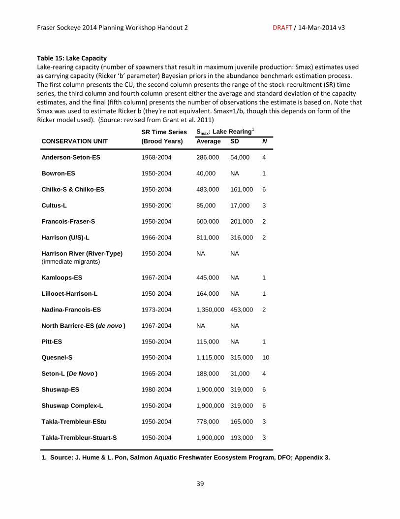
Fraser Sockeye 2014 Planning Workshop Handout 2 DRAFT / 14-Mar-2014 v3
39
Table 15: Lake Capacity Lake-rearing capacity (number of spawners that result in maximum juvenile production: Smax) estimates used as carrying capacity (Ricker ‘b’ parameter) Bayesian priors in the abundance benchmark estimation process. The first column presents the CU, the second column presents the range of the stock-recruitment (SR) time series, the third column and fourth column present either the average and standard deviation of the capacity estimates, and the final (fifth column) presents the number of observations the estimate is based on. Note that Smax was used to estimate Ricker b (they're not equivalent. Smax=1/b, though this depends on form of the Ricker model used). (Source: revised from Grant et al. 2011)
SR Time Series Smax: Lake Rearing1
CONSERVATION UNIT (Brood Years) Average SD N
Anderson-Seton-ES 1968-2004 286,000 54,000 4
Bowron-ES 1950-2004 40,000 NA 1
Chilko-S & Chilko-ES 1950-2004 483,000 161,000 6
Cultus-L 1950-2000 85,000 17,000 3
Francois-Fraser-S 1950-2004 600,000 201,000 2
Harrison (U/S)-L 1966-2004 811,000 316,000 2
Harrison River (River-Type) 1950-2004 NA NA
(immediate migrants)
Kamloops-ES 1967-2004 445,000 NA 1
Lillooet-Harrison-L 1950-2004 164,000 NA 1
Nadina-Francois-ES 1973-2004 1,350,000 453,000 2
North Barriere-ES (de novo ) 1967-2004 NA NA
Pitt-ES 1950-2004 115,000 NA 1
Quesnel-S 1950-2004 1,115,000 315,000 10
Seton-L (De Novo ) 1965-2004 188,000 31,000 4
Shuswap-ES 1980-2004 1,900,000 319,000 6
Shuswap Complex-L 1950-2004 1,900,000 319,000 6
Takla-Trembleur-EStu 1950-2004 778,000 165,000 3
Takla-Trembleur-Stuart-S 1950-2004 1,900,000 193,000 3
1. Source: J. Hume & L. Pon, Salmon Aquatic Freshwater Ecosystem Program, DFO; Appendix 3.
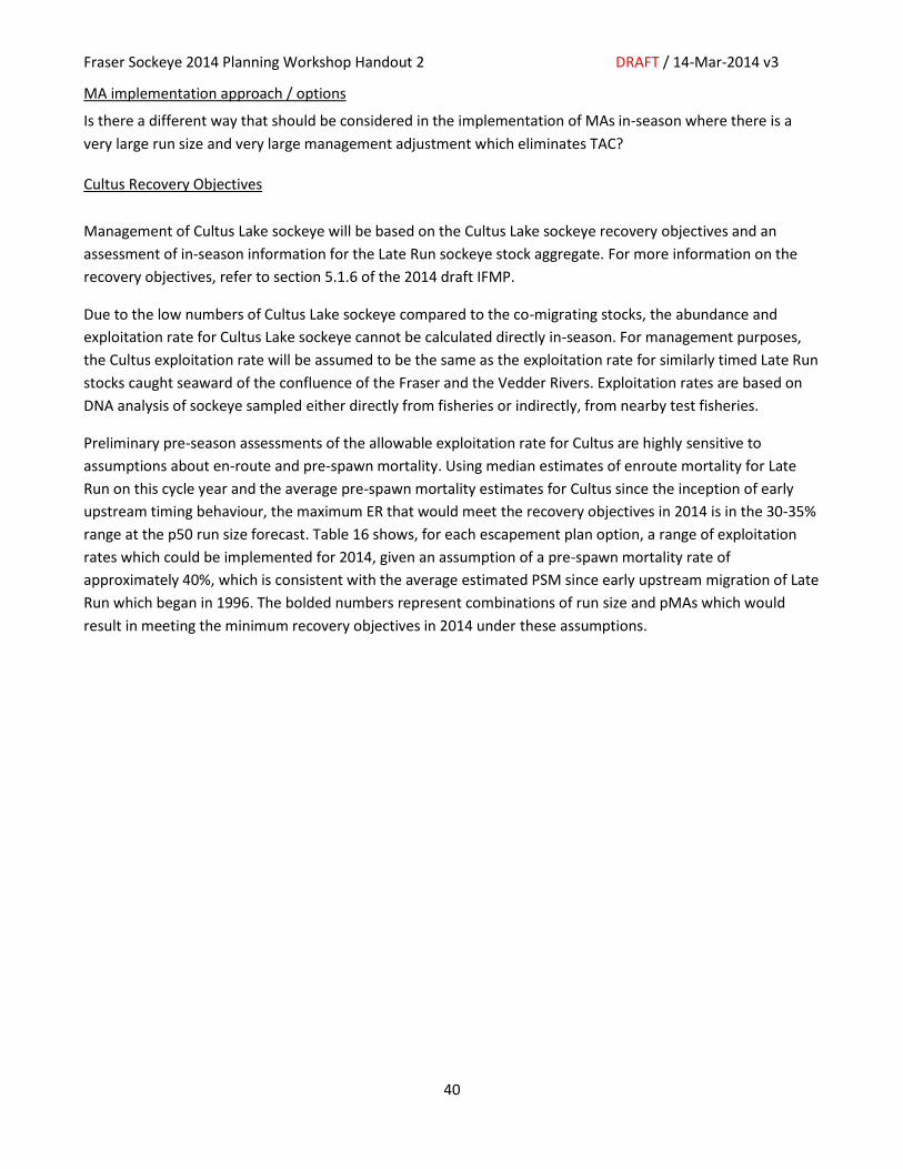
Fraser Sockeye 2014 Planning Workshop Handout 2 DRAFT / 14-Mar-2014 v3
40
MA implementation approach / options
Is there a different way that should be considered in the implementation of MAs in-season where there is a
very large run size and very large management adjustment which eliminates TAC?
Cultus Recovery Objectives
Management of Cultus Lake sockeye will be based on the Cultus Lake sockeye recovery objectives and an
assessment of in-season information for the Late Run sockeye stock aggregate. For more information on the
recovery objectives, refer to section 5.1.6 of the 2014 draft IFMP.
Due to the low numbers of Cultus Lake sockeye compared to the co-migrating stocks, the abundance and
exploitation rate for Cultus Lake sockeye cannot be calculated directly in-season. For management purposes,
the Cultus exploitation rate will be assumed to be the same as the exploitation rate for similarly timed Late Run
stocks caught seaward of the confluence of the Fraser and the Vedder Rivers. Exploitation rates are based on
DNA analysis of sockeye sampled either directly from fisheries or indirectly, from nearby test fisheries.
Preliminary pre-season assessments of the allowable exploitation rate for Cultus are highly sensitive to
assumptions about en-route and pre-spawn mortality. Using median estimates of enroute mortality for Late
Run on this cycle year and the average pre-spawn mortality estimates for Cultus since the inception of early
upstream timing behaviour, the maximum ER that would meet the recovery objectives in 2014 is in the 30-35%
range at the p50 run size forecast. Table 16 shows, for each escapement plan option, a range of exploitation
rates which could be implemented for 2014, given an assumption of a pre-spawn mortality rate of
approximately 40%, which is consistent with the average estimated PSM since early upstream migration of Late
Run which began in 1996. The bolded numbers represent combinations of run size and pMAs which would
result in meeting the minimum recovery objectives in 2014 under these assumptions.
Fraser Sockeye 2014 Planning Workshop Handout 2 DRAFT / 14-Mar-2014 v3
41
Table 16: Stock-specific Projection under Options 1 and 2 compared to high observations
A range of maximum exploitation rates for Cultus Sockeye which could be implemented for 2014 and would
meet minimum recovery objectives, assuming a pre-spawn mortality rate of approximately 40%
Option 1: Like Cycle Year
Option 2: Increase TAM Cap
Fraser Sockeye 2014 Planning Workshop Handout 2 DRAFT / 14-Mar-2014 v3
42
5. References
Cass A, M Folkes, G Pestal. 2004. Methods for assessing harvest rules for Fraser River sockeye salmon. DFO Can. Sci. Advis. Sec. Res. Doc. 2004/025. (Available on-line at www.dfo-mpo.gc.ca/csas/Csas/publications/ResDocs-DocRech/2004/2004_025_e.htm)
DFO. 2005. Canada’s policy for conservation of wild Pacific salmon. (Available on-line at:
www.pac.dfo-mpo.gc.ca/publications/pdfs/wsp-eng.pdf) DFO. 2006a. A harvest strategy compliant with the precautionary approach. DFO Can. Sci. Advis. Sec.
Sci. Advis. Rep. 2006/023. Available on-line at http://www.dfo-mpo.gc.ca/csas/Csas/status/2006/SAR-AS2006_023_E.pdf
DFO. 2006b. Workshop to assess population dynamics of cyclic Fraser River sockeye and implications
for management. DFO Can. Sci. Advis. Sec. Proceed. Ser. 2006/004. Available on-line at http://www.dfo-mpo.gc.ca/Library/324076.pdf
Grant S.C.H., B.L. MacDonald, T.E. Cone, C.A. Holt, A. Cass, E.J. Porszt, J.M.B. Hume, and L.B. Pon.
2011. Evaluation of Uncertainty in Fraser Sockeye (Oncorhynchus nerka) Wild Salmon Policy Status using Abundance and Trends in Abundance Metrics. DFO Can. Sci. Advis. Sec. Sci. Advis. Rep. 2011/087. Available on-line at http://www.dfo-mpo.gc.ca/Csas-sccs/publications/resdocs-docrech/2011/2011_087-eng.pdf
Pestal G, A-M Huang and AJ Cass. 2011. Updated Methods For Assessing Harvest Rules For Fraser
River Sockeye Salmon (Oncorhynchus nerka). DFO Can. Sci. Advis. Sec. Sci. Advis. Rep. 2011/133. Available on-line at http://www.dfo-mpo.gc.ca/csas-sccs/Publications/ResDocs-DocRech/2011/2011_133-eng.html
Pestal G, P Ryall, and AJ Cass. 2008. Collaborative Development of Escapement Strategies for Fraser
River Sockeye: Summary Report 2003 – 2008. Can. Man. Rep. Fish. Aquat. Sci. 2855: viii + 84 p. Available online at http://www.dfo-mpo.gc.ca/Library/334450.pdf