Embed Size (px)
Citation preview
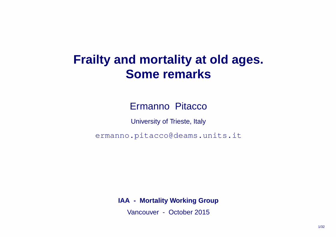
Frailty and mortality at old ages.Some remarks
Ermanno Pitacco
University of Trieste, Italy
IAA - Mortality Working Group
Vancouver - October 2015
1/32
– p. 1/32
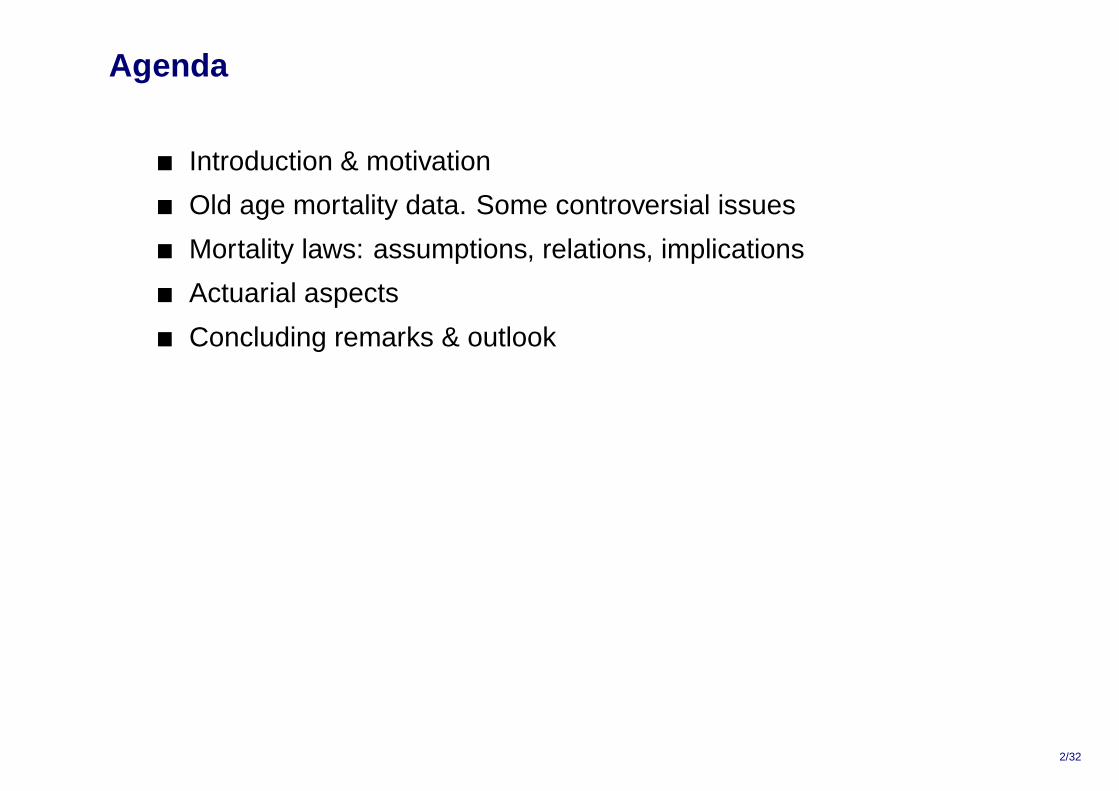
Agenda
� Introduction & motivation
� Old age mortality data. Some controversial issues
� Mortality laws: assumptions, relations, implications
� Actuarial aspects
� Concluding remarks & outlook
2/32
– p. 2/32

INTRODUCTION & MOTIVATION
Very extensive literature on mortality at old and very old ages, inparticular focussing on:
⊲ longevity limits (maximum length of life)
⊲ (possible) deceleration in the age-pattern of mortality at old and/orvery old ages
⊲ dynamic aspects, i.e. mortality trends
⊲ impact of heterogeneity
Research involving:
• demography
• actuarial sciences
• gerontology
• biology
• epidemiology
• . . . . . .3/32
– p. 3/32
Introduction & motivation (cont’d)
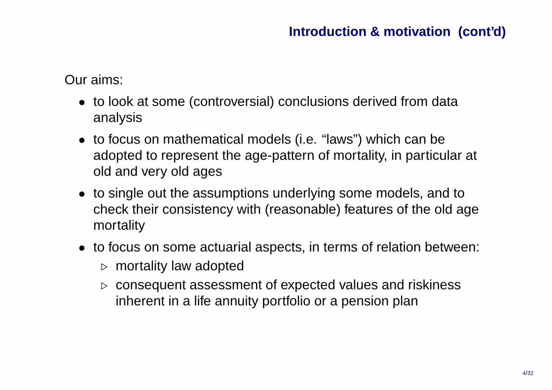
Our aims:
• to look at some (controversial) conclusions derived from dataanalysis
• to focus on mathematical models (i.e. “laws”) which can beadopted to represent the age-pattern of mortality, in particular atold and very old ages
• to single out the assumptions underlying some models, and tocheck their consistency with (reasonable) features of the old agemortality
• to focus on some actuarial aspects, in terms of relation between:⊲ mortality law adopted⊲ consequent assessment of expected values and riskiness
inherent in a life annuity portfolio or a pension plan
4/32
– p. 4/32

OLD AGE MORTALITY DATA.SOME CONTROVERSIAL ISSUES
Archive on population data on aging
See: Thatcher [1999]
Deaths at age 80 and over, in 30 countries, since 1960 (at least)
Database currently held at University of Odense and Max PlanckInstitute, Rostock
Data closer to the logistic model ( ⇒ heterogeneity), than to theGompertz model or the Weibull model
Three explanations suggested:
1. (fixed) individual frailty
2. stochastic process model ⇒ individuals moving through healthclasses
3. genetic
5/32
– p. 5/32

Old age mortality data. Some controversial issues (cont’d)
Mortality data of Sweden (1861 - 1990) and Japan (1951 - 1990)
See: Horiuchi and Wilmoth [1998]
Mortality data by cause of death (COD)
Deceleration can be explained by:
1. heterogeneity hypothesis ⇒ demographic explanation, relying onpopulation composition⊲ more frail individual tend to die earlier
2. individual-risk hypothesis ⇒ gerontological explanation, in termsof senescent process⊲ less energy expenditure⊲ more protected environment⊲ . . . . . .
Heterogeneity explored by Horiuchi and Wilmoth ⇒ heterogeneityhypothesis supported by results
6/32
– p. 6/32

Old age mortality data. Some controversial issues (cont’d)
New aspect singled out: timing of deceleration, i.e. when thedeceleration phase starts
Predictions about timing of deceleration can be made according toCODs
Three predictions proposed:
(a) deceleration due to “selective” CODs⇒ early
(b) deceleration due to most of CODs⇒ timing depends on individual vulnerability to diseases which
constitute CODs
(c) deceleration due to overall mortality (all CODs aggregated)⇒ late
7/32
– p. 7/32
Old age mortality data. Some controversial issues (cont’d)
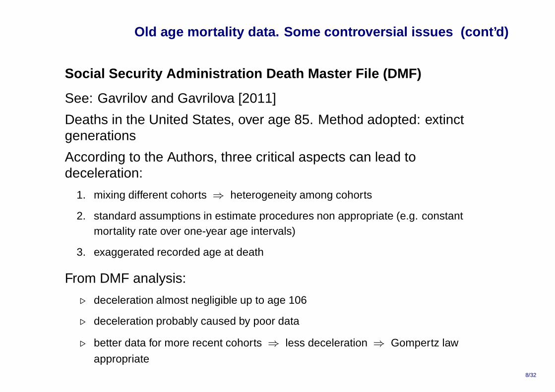
Social Security Administration Death Master File (DMF)
See: Gavrilov and Gavrilova [2011]
Deaths in the United States, over age 85. Method adopted: extinctgenerations
According to the Authors, three critical aspects can lead todeceleration:
1. mixing different cohorts ⇒ heterogeneity among cohorts
2. standard assumptions in estimate procedures non appropriate (e.g. constantmortality rate over one-year age intervals)
3. exaggerated recorded age at death
From DMF analysis:
⊲ deceleration almost negligible up to age 106
⊲ deceleration probably caused by poor data
⊲ better data for more recent cohorts ⇒ less deceleration ⇒ Gompertz law
appropriate8/32
– p. 8/32

MORTALITY LAWS:ASSUMPTIONS, RELATIONS, IMPLICATIONS
Mortality laws vs polynomial and spline graduation
Biological, physiological and possibly behavioral assumptions underpinmany mortality laws, or components of mortality laws
Polynomial and splines graduations:
⊲ only aim at fitting and smoothing
⊲ also adopted to extrapolate age pattern of mortality beyond agesfor which reliable observations are available
Remark
Linking basic biology of humans to life table functions first proposed byGompertz, 1825, and Brownlee, 1919; see Olshansky and Carnes [1997]
9/32
– p. 9/32
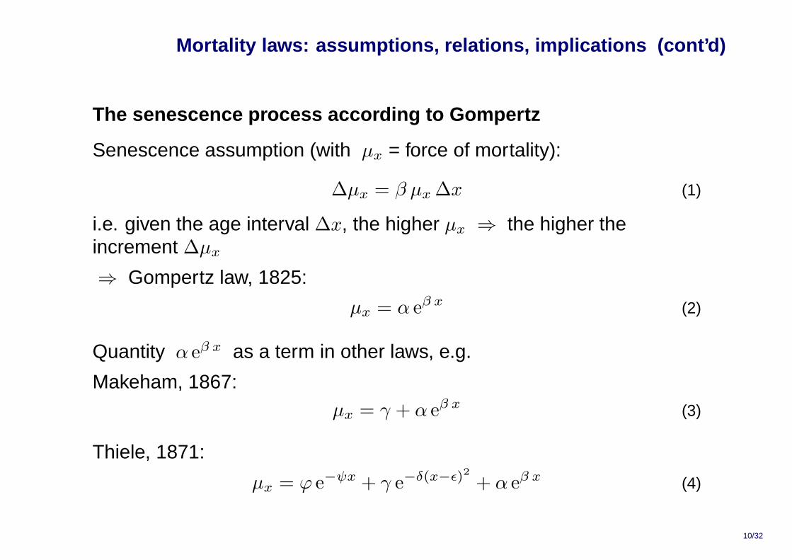
Mortality laws: assumptions, relations, implications (cont’d)
The senescence process according to Gompertz
Senescence assumption (with µx = force of mortality):
∆µx = β µx∆x (1)
i.e. given the age interval ∆x, the higher µx ⇒ the higher theincrement ∆µx
⇒ Gompertz law, 1825:
µx = α eβ x (2)
Quantity α eβ x as a term in other laws, e.g.
Makeham, 1867:µx = γ + α eβ x (3)
Thiele, 1871:
µx = ϕ e−ψx + γ e−δ(x−ǫ)2
+ α eβ x (4)
10/32
– p. 10/32
Mortality laws: assumptions, relations, implications (cont’d)
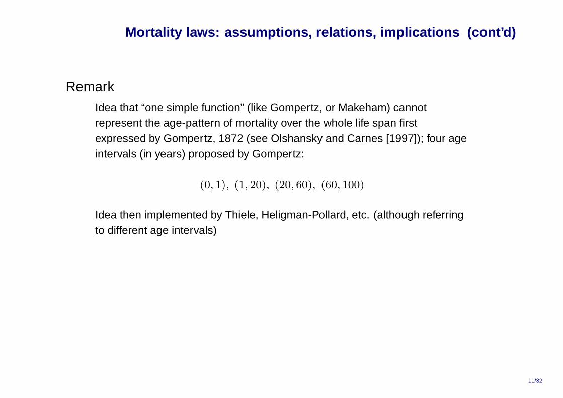
Remark
Idea that “one simple function” (like Gompertz, or Makeham) cannotrepresent the age-pattern of mortality over the whole life span firstexpressed by Gompertz, 1872 (see Olshansky and Carnes [1997]); four ageintervals (in years) proposed by Gompertz:
(0, 1), (1, 20), (20, 60), (60, 100)
Idea then implemented by Thiele, Heligman-Pollard, etc. (although referringto different age intervals)
11/32
– p. 11/32
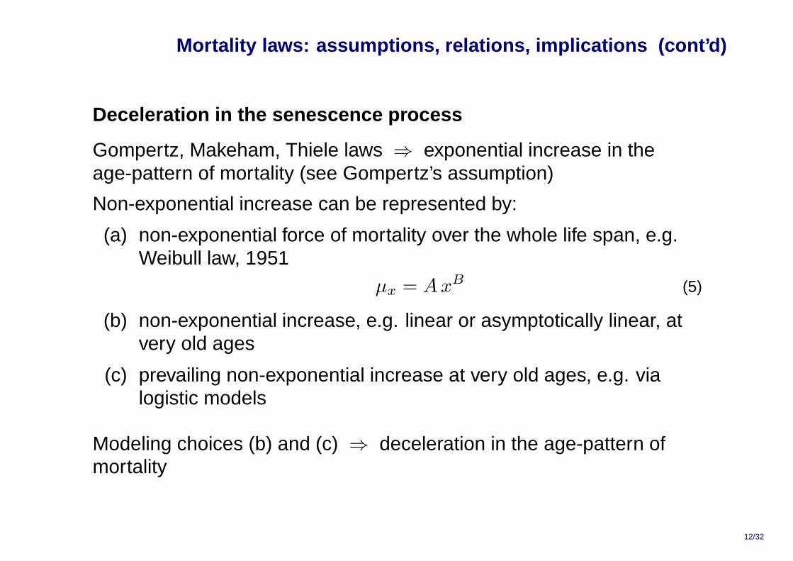
Mortality laws: assumptions, relations, implications (cont’d)
Deceleration in the senescence process
Gompertz, Makeham, Thiele laws ⇒ exponential increase in theage-pattern of mortality (see Gompertz’s assumption)
Non-exponential increase can be represented by:
(a) non-exponential force of mortality over the whole life span, e.g.Weibull law, 1951
µx = A xB (5)
(b) non-exponential increase, e.g. linear or asymptotically linear, atvery old ages
(c) prevailing non-exponential increase at very old ages, e.g. vialogistic models
Modeling choices (b) and (c) ⇒ deceleration in the age-pattern ofmortality
12/32
– p. 12/32
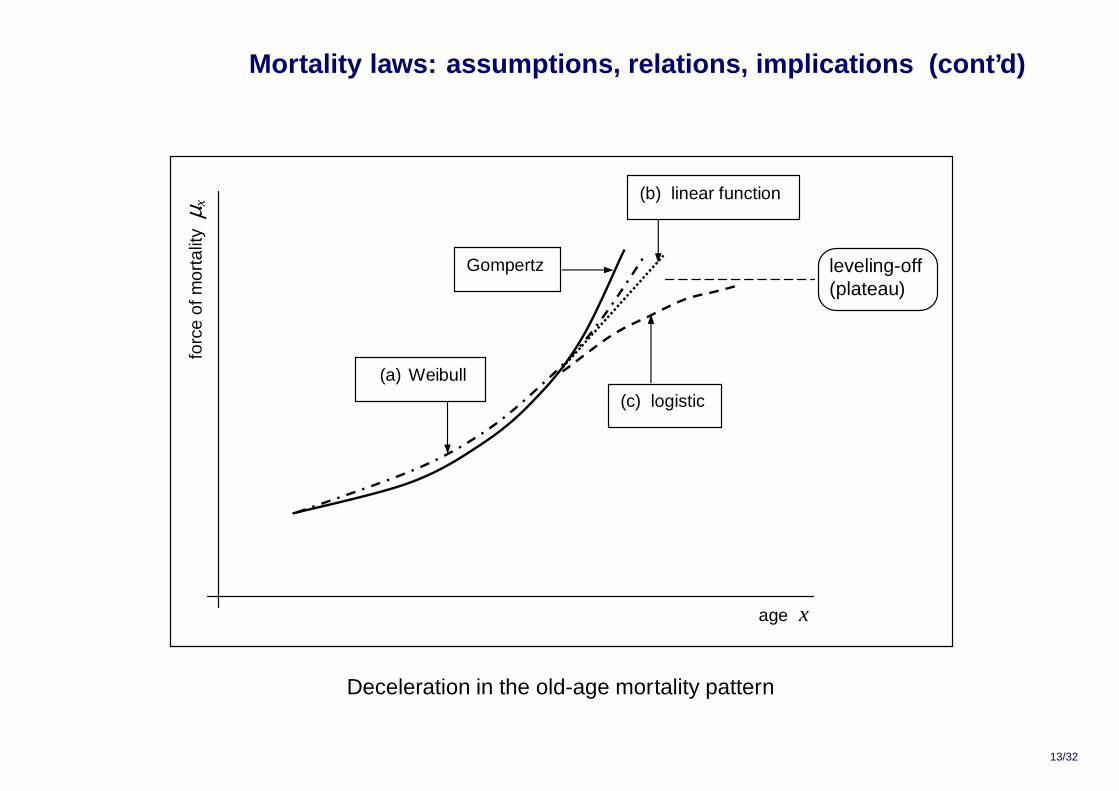
Mortality laws: assumptions, relations, implications (cont’d)
age x
forc
e of
mor
talit
y µ
x
Gompertz
(c) logistic
(b) linear function
leveling-off (plateau)
(a) Weibull
Deceleration in the old-age mortality pattern
13/32
– p. 13/32
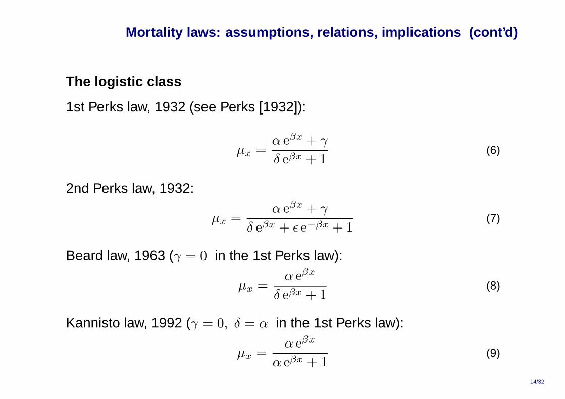
Mortality laws: assumptions, relations, implications (cont’d)
The logistic class
1st Perks law, 1932 (see Perks [1932]):
µx =α eβx + γ
δ eβx + 1(6)
2nd Perks law, 1932:
µx =α eβx + γ
δ eβx + ǫ e−βx + 1(7)
Beard law, 1963 (γ = 0 in the 1st Perks law):
µx =α eβx
δ eβx + 1(8)
Kannisto law, 1992 (γ = 0, δ = α in the 1st Perks law):
µx =α eβx
α eβx + 1(9)
14/32
– p. 14/32
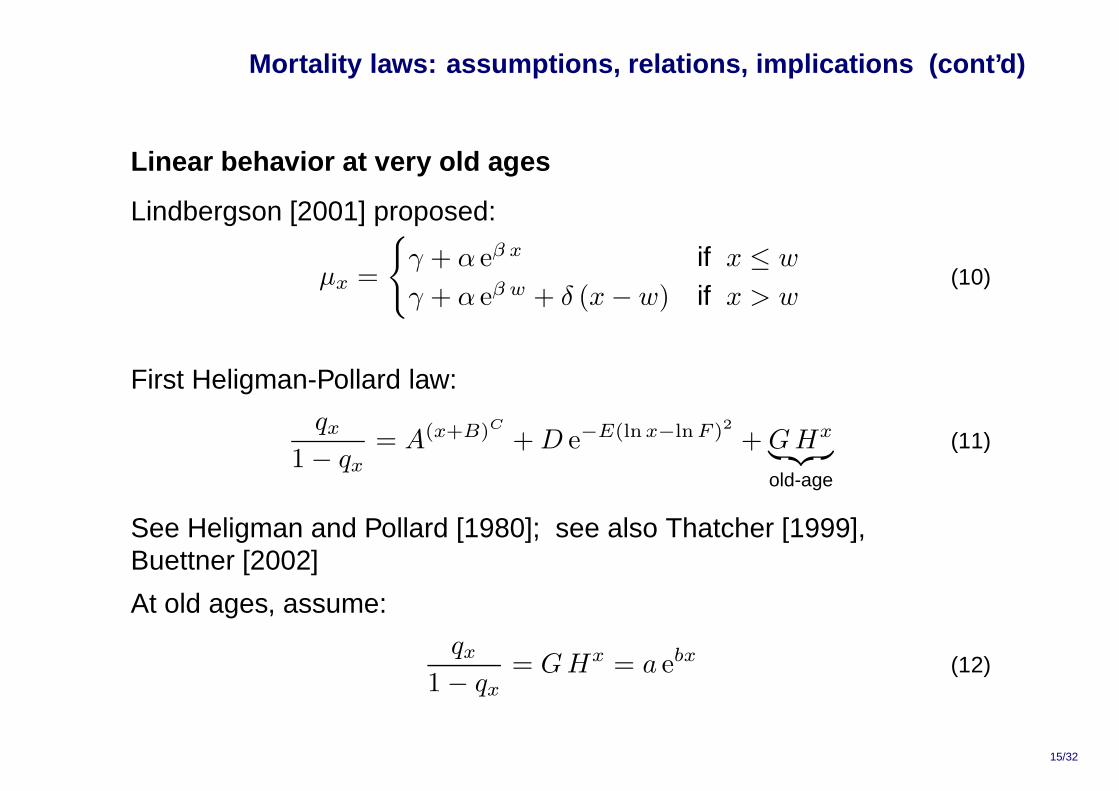
Mortality laws: assumptions, relations, implications (cont’d)
Linear behavior at very old ages
Lindbergson [2001] proposed:
µx =
{
γ + α eβ x if x ≤ w
γ + α eβ w + δ (x − w) if x > w(10)
First Heligman-Pollard law:
qx
1 − qx= A(x+B)C
+ D e−E(lnx−lnF )2 + GHx
︸ ︷︷ ︸
old-age
(11)
See Heligman and Pollard [1980]; see also Thatcher [1999],Buettner [2002]
At old ages, assume:
qx
1 − qx= GHx = a ebx (12)
15/32
– p. 15/32
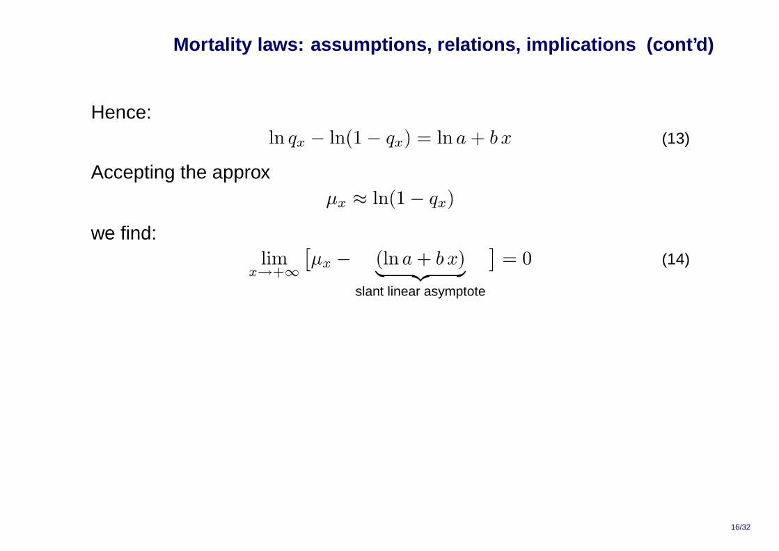
Mortality laws: assumptions, relations, implications (cont’d)
Hence:ln qx − ln(1 − qx) = ln a + b x (13)
Accepting the approxµx ≈ ln(1 − qx)
we find:lim
x→+∞
[µx − (ln a + b x)
︸ ︷︷ ︸
slant linear asymptote
]= 0 (14)
16/32
– p. 16/32

Mortality laws: assumptions, relations, implications (cont’d)
The Coale-Kisker assumption
See: Coale and Kisker [1990]. See also: Buettner [2002],Wilmoth [1995]
Model relying on the exponential age-specific rate of change of centraldeath rates:
kx = lnmx
mx−1(15)
Assumption: kx linear over age 85
kx = k85 − (x − 85) s (16)
Parameter s calculated
⊲ assuming k85 determined from empirical data
⊲ assigning a predetermined value to m110
17/32
– p. 17/32

Mortality laws: assumptions, relations, implications (cont’d)
We find from (15):
mx = m85 exp
(x∑
h=86
kh
)
(17)
and from (17):
mx = ea x2+b x+c (18)
The model can be used to extrapolate the age pattern of mortalitybeyond ages for which reliable observations are available
18/32
– p. 18/32
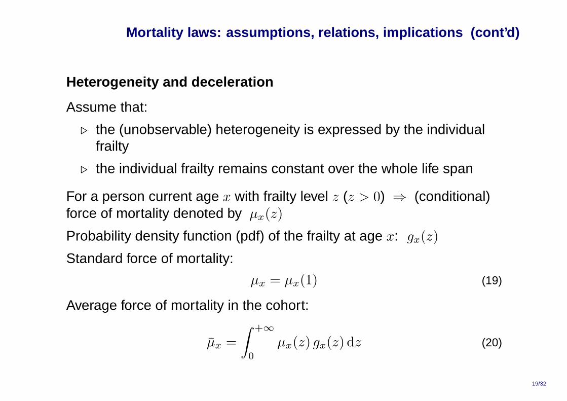
Mortality laws: assumptions, relations, implications (cont’d)
Heterogeneity and deceleration
Assume that:
⊲ the (unobservable) heterogeneity is expressed by the individualfrailty
⊲ the individual frailty remains constant over the whole life span
For a person current age x with frailty level z (z > 0) ⇒ (conditional)force of mortality denoted by µx(z)
Probability density function (pdf) of the frailty at age x: gx(z)
Standard force of mortality:
µx = µx(1) (19)
Average force of mortality in the cohort:
µ̄x =
∫ +∞
0
µx(z) gx(z) dz (20)
19/32
– p. 19/32
Mortality laws: assumptions, relations, implications (cont’d)
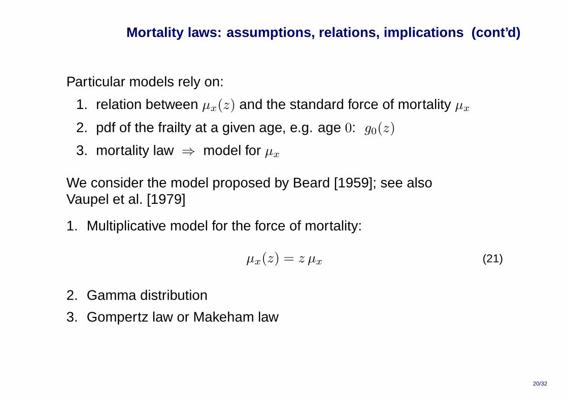
Particular models rely on:
1. relation between µx(z) and the standard force of mortality µx
2. pdf of the frailty at a given age, e.g. age 0: g0(z)
3. mortality law ⇒ model for µx
We consider the model proposed by Beard [1959]; see alsoVaupel et al. [1979]
1. Multiplicative model for the force of mortality:
µx(z) = z µx (21)
2. Gamma distribution
3. Gompertz law or Makeham law
20/32
– p. 20/32
Mortality laws: assumptions, relations, implications (cont’d)
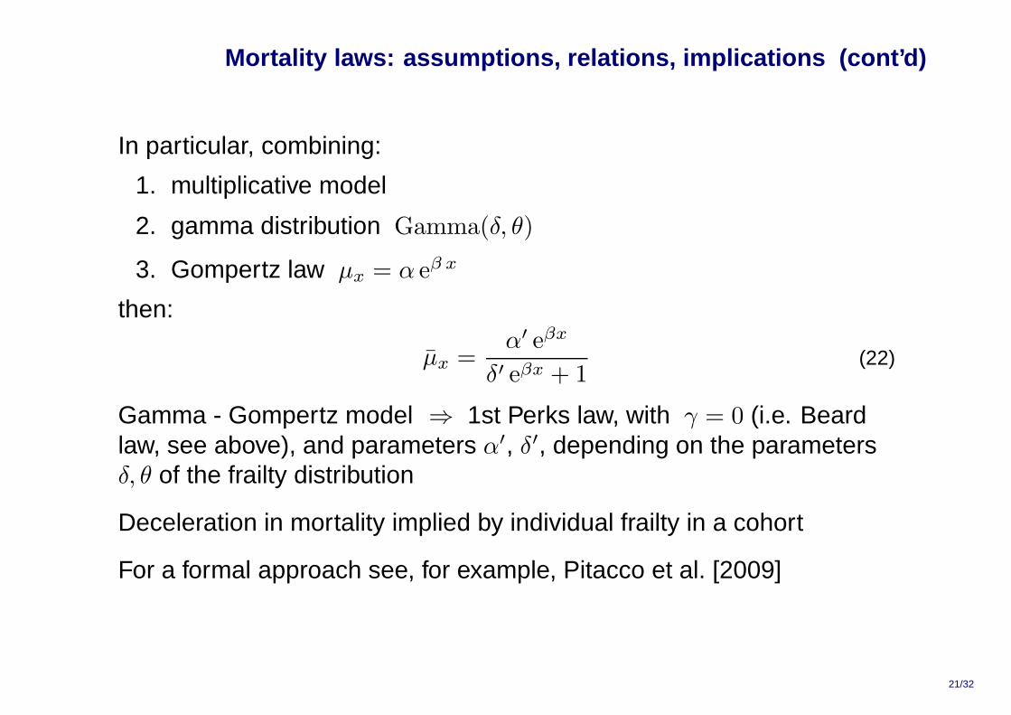
In particular, combining:
1. multiplicative model
2. gamma distribution Gamma(δ, θ)
3. Gompertz law µx = α eβ x
then:
µ̄x =α′ eβx
δ′ eβx + 1(22)
Gamma - Gompertz model ⇒ 1st Perks law, with γ = 0 (i.e. Beardlaw, see above), and parameters α′, δ′, depending on the parametersδ, θ of the frailty distribution
Deceleration in mortality implied by individual frailty in a cohort
For a formal approach see, for example, Pitacco et al. [2009]
21/32
– p. 21/32
Mortality laws: assumptions, relations, implications (cont’d)
Actuarial research on heterogeneity, frailty and related impacts⇒ see, for example: Butt and Haberman [2002, 2004], Olivieri [2006],
Meyricke and Sherris [2013]
Remark
Logistic model for the average force of mortality, µ̄x, can be the result ofother assumptions, for example the stochastic process of ageing proposedby Le Bras [1976]:
⊲ cohort homogeneous at birth ⇒ all its members were in the samestate of health
⊲ people move from one state of health to another ⇒ heterogeneity thendevelops during life
See also: Thatcher et al. [1998], Thatcher [1999]
22/32
– p. 22/32
ACTUARIAL ASPECTS
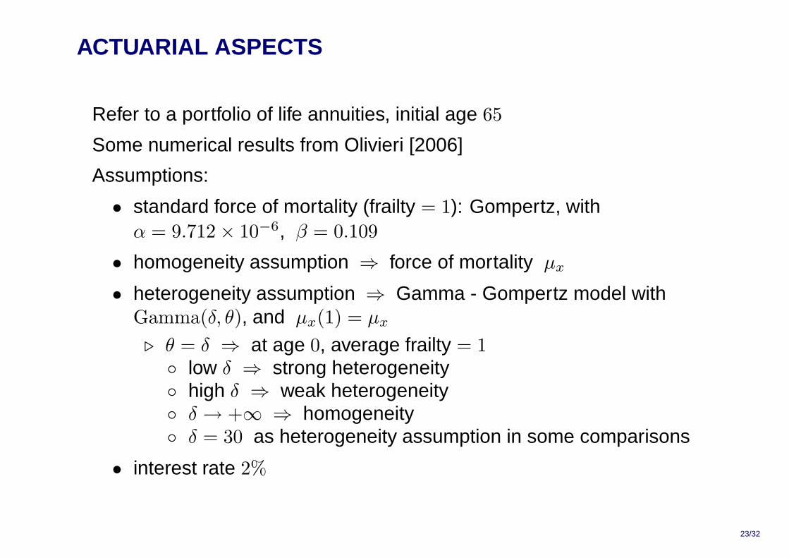
Refer to a portfolio of life annuities, initial age 65
Some numerical results from Olivieri [2006]
Assumptions:
• standard force of mortality (frailty = 1): Gompertz, withα = 9.712 × 10⁻⁶, β = 0.109
• homogeneity assumption ⇒ force of mortality µx
• heterogeneity assumption ⇒ Gamma - Gompertz model withGamma(δ, θ), and µx(1) = µx
⊲ θ = δ ⇒ at age 0, average frailty = 1◦ low δ ⇒ strong heterogeneity◦ high δ ⇒ weak heterogeneity◦ δ → +∞ ⇒ homogeneity◦ δ = 30 as heterogeneity assumption in some comparisons
• interest rate 2%
23/32
– p. 23/32
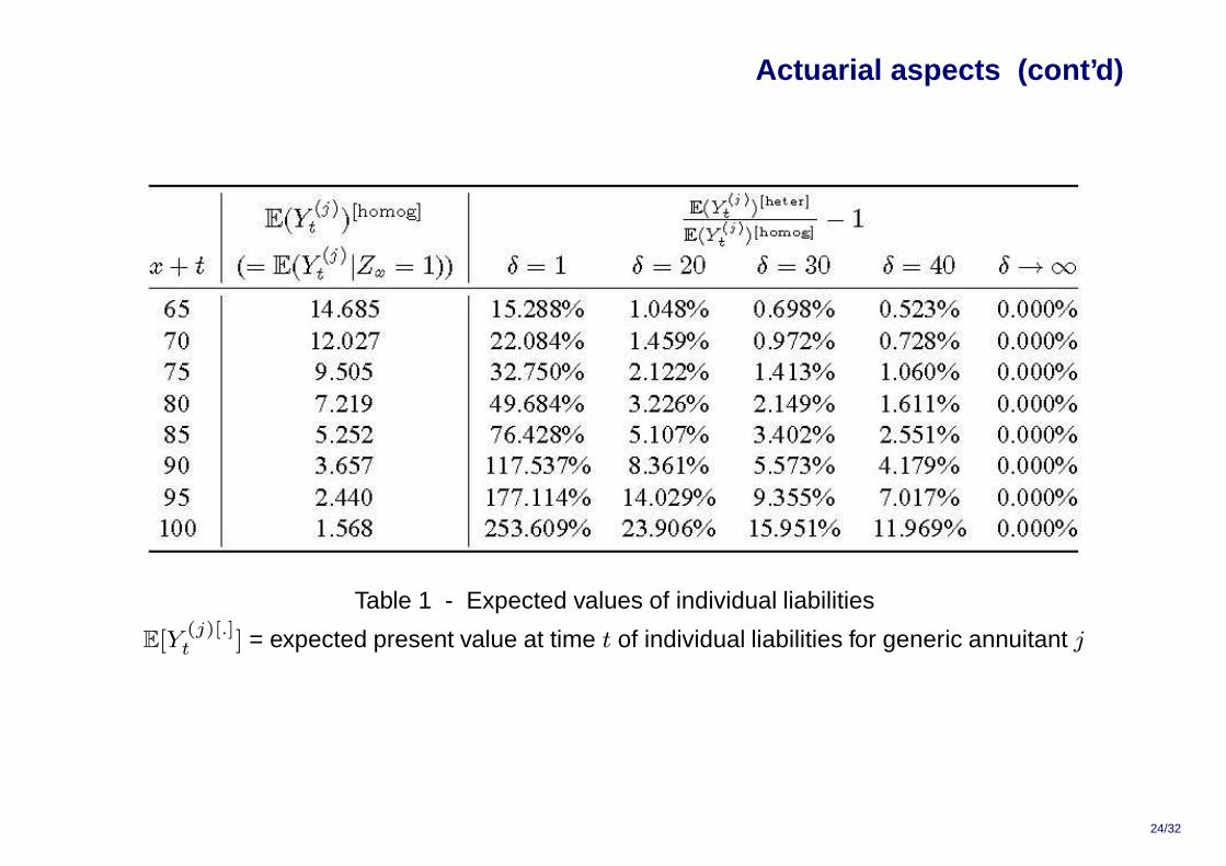
Actuarial aspects (cont’d)
Table 1 - Expected values of individual liabilities
E[Y(j)[.]t ] = expected present value at time t of individual liabilities for generic annuitant j
24/32
– p. 24/32

Actuarial aspects (cont’d)
size ntx = 65 x + 10 = 75 x + 20 = 85
[homog] [heter] [homog] [heter] [homog] [heter]
10 12.757% 14.921% 16.528% 20.367% 20.846% 27.092%
1 000 1.276% 8.090% 1.653% 12.467% 2.085% 18.173%
10 000 0.403% 8.001% 0.523% 12.372% 0.659% 18.071%
Table 2 - Coefficient of variation of liabilities for some portfolios
From numerical results
⊲ Table 1: disregarding heterogeneity ⇒ underestimation of theexpected present values (and hence of the reserves)
⊲ Table 2: disregarding heterogeneity ⇒ underestimation of the(relative) riskiness in the portfolio (and hence of capitalrequirements)
25/32
– p. 25/32

CONCLUDING REMARKS & OUTLOOK
Various causes of wrong estimation of the age pattern of mortality
A possible cause: heterogeneity, due to:
(a) mixing several cohorts data
(b) heterogeneity among individuals in one cohort, in particularindividual frailty
From an actuarial perspective: disregarding (b) ⇒ underestimation of
⊲ expected values ( ⇒ pricing, reserving)
⊲ risk ( ⇒ risk margin, capital allocation)
26/32
– p. 26/32

Concluding remarks & outlook (cont’d)
Individual frailty Mixing cohorts in mortality analysis
Heterogeneity (one-cohort population)
Heterogeneity (multiple-cohort
population)
Logistic models
Deceleration in the age-pattern of mortality
Higher volatility in: - number of survivors - cash flows of life annuity
portfolios
Causes
Primary effect
Appropriate modeling
Secondary effects
Heterogeneity, Deceleration, Volatility
27/32
– p. 27/32

Concluding remarks & outlook (cont’d)
Further steps (in collaboration with Annamaria Olivieri, University ofParma)
• Risk assessment ⇒ probability distribution of lifetimes, andrelated typical values (expected value, modal value, variance,etc.) under various mortality assumptions
• Impact assessment ⇒ DCF model to quantify liability valuesunder various mortality assumptions
28/32
– p. 28/32

References
Where links are provided, they were active as of the time this presentationwas completed but may have been updated since then.
R. E. Beard. Note on some mathematical mortality models. In C. E. W. Wolstenholmeand M. O. Connor, editors, CIBA Foundation Colloquia on Ageing, volume 5, pages302–311, Boston, 1959
T. Buettner. Approaches and experiences in projecting mortality patterns for theoldest-old. North American Actuarial Journal, 6(3):14–25, 2002
Z. Butt and S. Haberman. Application of frailty-based mortality models to insurance data.Actuarial Research Paper 142, Dept. of Actuarial Science and Statistics, City University,London, 2002
Z. Butt and S. Haberman. Application of frailty-based mortality models using generalizedlinear models. ASTIN Bulletin, 34(1):175–197, 2004
A. Coale and E. Kisker. Defects in data on old age mortality in the United States: Newprocedures for calculating approximately accurate mortality schedules and life tables atthe highest ages. Asian and Pacific Population Forum, 4:1–31, 1990
29/32
– p. 29/32

References (cont’d)
L. G. Doray. Inference for logistic-type models for the force of mortality. Presented at theLiving to 100 and Beyond Symposium. Orlando, FL, 2008. Available at:https://www.soa.org/library/monographs/retirement-systems/
living-to-100-and-beyond/2008/january/subject-toc.aspx
L. A. Gavrilov and N. S. Gavrilova. Mortality measurement at advanced ages: A study ofthe Social Security Administration Death Master File. North American Actuarial Journal,15(3):432–447, 2011
S. Horiuchi and J. R. Wilmoth. Deceleration in the age pattern of mortality at older ages.Demography, 35(4):391–412, 1998
V. Kannisto. Development of Oldest-Old Mortality, 1950-1990: Evidence from 28Developed Countries. Odense Monograph on Population Aging, 1. Odense UniversityPress, 1994. Available at:http://www.demogr.mpg.de/Papers/Books/Monograph1/OldestOld.htm
H. Le Bras. Lois de mortalité et age limite. Population, 31(3):655–692, 1976
M. Lindbergson. Mortality among the elderly in Sweden 1988-97. ScandinavianActuarial Journal, (1):79–94, 2001
30/32
– p. 30/32

References (cont’d)
R. Meyricke and M. Sherris. The determinants of mortality heterogeneity andimplications for pricing annuities. Insurance: Mathematics & Economics, 53(2):379–387,2013
A. Olivieri. Heterogeneity in survival models. applications to pension and life annuities.Belgian Actuarial Bulletin, 6:23–39, 2006. Available at:http://www.actuaweb.be/frameset/frameset.html
S. J. Olshansky and B. E. Carnes. Ever since Gompertz. Demography, 34(1):1–15, 1997
W. Perks. On some experiments in the graduation of mortality statistics. Journal of theInstitute of Actuaries, 63:12–57, 1932
E. Pitacco, M. Denuit, S. Haberman, and A. Olivieri. Modelling Longevity Dynamics forPensions and Annuity Business. Oxford University Press, 2009
A. R. Thatcher. The long-term pattern of adult mortality and the highest attained age.Journal of the Royal Statistical Society, A, 162:5–43, 1999
A. R. Thatcher, V. Kannisto, and J. W. Vaupel. The Force of Mortality at Ages 80 to 120.Odense Monograph on Population Aging, 5. Odense University Press, 1998. Availableat: http://www.demogr.mpg.de/Papers/Books/Monograph5/start.htm
31/32
– p. 31/32
References (cont’d)
J. W. Vaupel, K. G. Manton, and E. Stallard. The impact of heterogeneity in individualfrailty on the dynamics of mortality. Demography, 16(3):439–454, 1979
J. R. Wilmoth. Are mortality rates falling at extremely high ages? An investigation basedon a model proposed by Coale and Kisker. Population Studies, 49(2):281–295, 1995
32/32
– p. 32/32


![Frailty pathway [970kb]](https://img.dokumen.tips/doc/110x75/588da5761a28ab737b8b4e2c/frailty-pathway-970kb.jpg)


