Fourier Series Expansion in a Non-Orthogonal

System of Coordinates for the Simulation of

3D Alternating Current Borehole Resistivity

Measurements

D. Pardo[a], C. Torres-Verdın[a], M. J. Nam[a],M. Paszynski[b], and V. M. Calo[c]

aDepartment of Petroleum and Geosystems Engineering, The University of Texasat Austin

bDepartment of Computer Science, AGH University of Technology, Krakow,Poland

cInstitute for Computational Engineering and Sciences (ICES), The University ofTexas at Austin

Abstract

We describe a method to simulate 3D resistivity borehole measurements acquiredwith alternating current (AC) logging instruments. It combines the use of a Fourierseries expansion in a non-orthogonal system of coordinates with an existing 2Dgoal-oriented higher-order self-adaptive hp-Finite Element (FE) algorithm.

The method is used to simulate measurements acquired with both wireline andlogging-while-drilling (LWD) borehole logging instruments in deviated wells. It en-ables a considerable reduction of the computational complexity with respect toavailable 3D simulators, since the number of Fourier modes (basis functions) neededto solve practical applications is limited (typically, below 13). The fast convergenceof the method is studied via numerical experimentation by simulating two wirelineand one LWD instruments in a deviated well across a possibly invaded formation.

Numerical results confirm the efficiency and reliability of the method for sim-ulating challenging 3D AC resistivity borehole problems in deviated wells, whileavoiding the expensive construction of optimal 3D grids. We accurately simulatechallenging electrodynamic problems within a few seconds (or minutes) of CPUtime per logging position.

The method is especially well-suited for inversion of triaxial electromagnetic (EM)measurements, since we demonstrate that the number of Fourier modes needed forthe exact representation of the material function is limited to only one (the centralmode) for the case of borehole measurements acquired in deviated wells.

Key words: Fourier Series Expansion, Electromagnetism, hp-FE Method,

Preprint submitted to Elsevier 14 February 2008

Goal-Oriented Adaptivity, AC Borehole Measurements

1 Introduction

Resistivity logging instruments have been used during the last eighty yearsto quantify the spatial distribution of electrical conductivity in the vicinity ofboreholes. Conductivity of the rock formation is utilized to asses the materialproperties of the subsurface, and is routinely used by oil-companies to estimatethe volume of hydrocarbons (oil and gas) existing in a reservoir.

A variety of logging instruments have been employed to estimate the electricalconductivity of rock formations. In this paper, we focus on EM devices operat-ing at one or several specific frequencies. Almost all existing resistivity logginginstruments operate at particular frequencies, and therefore, are governed bythe time-harmonic Maxwell’s equations.

To improve the interpretation of results obtained with EM logging instru-ments, and thus, to better quantify and determine existing subsurface materi-als and increase hydrocarbon recovery, diverse methods have been developedto perform numerical simulations as well as to invert well-log measurements.In [1], we described a numerical method based on a Fourier series expansionin a non-orthogonal system of coordinates combined with a 2D self-adaptivehp goal-oriented Finite Element (FE) method. This method was formulatedand applied to direct-current (DC) resistivity problems, and it enabled fastand accurate simulations of previously unsolved EM simulation problems indeviated wells.

In this paper, we extend the numerical method presented in [1] to alternatingcurrent (AC) resistivity logging instruments, which operate at non-zero fre-quencies. The proposed method entails the use of a change of variables anda Fourier-Finite Element Method [2,3]. In addition, we illustrate the conver-gence properties of our method when applied to challenging borehole loggingproblems. The extension of the method described in [1] to 3D AC problems isnon-trivial, and it involves the following challenges:

• Derivation of time-harmonic variational formulation of Maxwell’s equationsin an arbitrary system of coordinates.

• Implementation of mixed variational formulations involving simultaneouslythe use of H(curl) and H1 FE discretizations.

• Development of a parallel implementation and fast direct solvers to reducethe CPU time and meet the increased memory requirements needed bysimulations of challenging AC logging measurements.

2

We emphasize that while DC simulations utilize a single scalar-valued variable(the scalar potential), AC simulations require the use of three vector-valuedvariables, corresponding to three components of the EM fields. In addition,the final variational formulation we obtain for AC problems with our methodis neither Hermitian nor complex-symmetric 1 . As a result, the computationalcost associated with simulations of AC measurements increases by approxi-mately one order of magnitude with respect to that associated with simula-tions of DC measurements.

Other numerical methods developed by the oil industry for simulations of ACresistivity logging instruments include fast 1D and 2D axial-symmetric sim-ulators such as, for example, those described in [4–7]. These simulators areunable to solve problems involving deviated wells 2 , due to the dimensionalityreduction. By contrast, 3D algorithms such as those described in [8–14,?,15]are capable of simulating resistivity measurements acquired in deviated wells.However, existing 3D simulators are not widely used by the logging industryin everyday logging-operations, either because the accuracy of these meth-ods is compromised and/or the CPU time required for simulations exceedsreasonable limits (several hours per logging position).

The method described in this paper provides highly accurate and reliableresults within reasonable CPU times as it enables a significant reduction of thecomputational complexity with respect to conventional 3D simulators withoutsacrifice of accuracy. In addition, the method is suitable for inverse problems,as well as for multi-physics applications. Therefore, it aims to become a widelyused simulation strategy for problems arising in the well-logging industry.

The remainder of this paper is organized as follows: In Section 2 we introduceMaxwell’s equations with appropriate boundary conditions. Then, we describeour method for AC problems and provide a formal derivation of our final vari-ational formulation. Implementation details of the method are described inSection 3. Numerical results included in Section 4 are focused toward val-idating the method and studying its applicability to everyday well-loggingoperations. Finally, Section 5 summarizes the main conclusions of this paper.

2 Method

In this Section, we first introduce Maxwell’s equations and we discuss the ap-propriate boundary conditions. Second, we derive a variational formulation for

1 For DC problems, we obtain a Hermitian variational formulation, see [1].2 Nowadays, most wells are deviated, since they may extend over longer distanceswithin the hydrocarbon layers, thereby enhancing hydrocarbon recovery.

3

3D time-harmonic Maxwell’s equations in an arbitrary system of coordinates(ζ1, ζ2, ζ3). Third, we assume that the solution in one of the directions in thenew coordinate system, e.g. ζ2, is periodic (for example, with period [0,2π]).Under this assumption, we employ a Fourier series expansion in terms of ζ2

to derive the corresponding variational formulation in terms of the Fouriermodal coefficients. Then, we consider the following non-orthogonal system ofcoordinates described in [1] (see also Fig. 1) for deviated wells in a boreholeenvironment:

x1 = ζ1 cos ζ2

x2 = ζ1 sin ζ2

x3 = ζ3 + θ0f(ζ1) cos ζ2

; f(ζ1) =

0 ζ1 < ρ1

ζ1 − ρ1

ρ2 − ρ1

ρ2 ρ1 ≤ ζ1 ≤ ρ2

ζ1 ζ1 > ρ2

, (1)

where θ0 = tan θ, θ is the dip angle 3 , and ρ1, ρ2 are given (constant) valuesthat depend upon each specific simulation problem.

QQsζ1

6

ζ3

ζ2

ζ2

6x1

-

x3cx2

Fig. 1. Cross section showing the 3D geometry of a resistivity logging instrumentin a vertical well penetrating dipping layers. Oblique circles indicate the “quasi-az-imuthal” direction ζ2 in the non-orthogonal system of coordinates (ζ1, ζ2, ζ3).

The above coordinate system verifies the assumption stated above (i.e. thesolution is periodic with respect to variable ζ2, with period length equal to2π) and, furthermore, requires only a few Fourier modes to represent exactlythe change of coordinates and the material coefficients. Finally, we brieflydescribe the method employed for solving the resulting formulation via a2D self-adaptive goal-oriented hp-FE method with variable order H1- andH(curl)-discretizations.

3 The dip angle is the angle between the well trajectory and a normal vector to thelayer boundaries.

4

2.1 Time-Harmonic Maxwell’s Equations

Assuming a time-harmonic dependence of the form ejωt, with ω denoting an-gular frequency, Maxwell’s equations in linear media can be written as

∇×H = (σ + jωε)E + Jimp Ampere’s Law,

∇× E = −jωµH−Mimp Faraday’s Law,

∇ · (εE) = ρe Gauss’ Law of Electricity, and

∇ · (µH) = 0 Gauss’ Law of Magnetism.

(2)

In the above equations, H and E denote the magnetic and electric fields, re-spectively, real-valued tensors ε,µ, and σ stand for dielectric permittivity,magnetic permeability, and electrical conductivity of the media, respectively,ρe denotes the electric charge distribution, and Jimp,Mimp are representationsfor the prescribed, impressed electric and magnetic current sources, respec-tively. We assume that det(µ) 6= 0, and det(σ + jωε) 6= 0.

By taking the divergence of Faraday’s law, and applying Gauss’ Law of mag-netism, we find that Mimp is divergence free. We also emphasize that, asexplained in [16], impressed currents are only mathematical symbols utilizedto represent sources. However, we note that it may be impossible to realizearbitrary sources in practice. In particular, Mimp = 0 at zero-frequency isnon-physical, since Mimp is always proportional to the frequency of operation.

2.1.1 Boundary Conditions (BCs)

There exist a variety of BCs that can be incorporated into Maxwell’s equations.In the following, we describe those BCs that are of interest to the boreholelogging applications discussed in this paper.

2.1.1.1 Perfect Electric Conductor (PEC). A PEC is an idealizationof a highly conductive medium, that is, σ → ∞. The corresponding electricfield E converges to zero by applying Ampere’s law since, due to physicalconsiderations, we assume that σE, εE, Jimp ∈ L2(Ω). In the absence of im-pressed magnetic surface currents, Faraday’s law implies that the tangentialcomponent of E and the normal component of µH must remain continuousacross material interfaces. Consequently, the tangential component of the elec-tric field and the normal component of the magnetic field must vanish along

5

the PEC boundary, i.e.,

n×E = 0 ; n ·H = 0 , (3)

where n is the unit normal (outward) vector. The tangential component ofthe magnetic field (surface current) and the normal component of the electricfield (surface charge density) need not to be zero, and may be determineda-posteriori.

2.1.1.2 Source Antennas. Antennas are modeled by prescribing an im-pressed volume current Jimp or Mimp. Using the equivalence principle (see, forexample, [16]), one can replace the original impressed volume currents withthe following equivalent surface currents (see [17] for details):

JimpS = [n×H]S ; Mimp

S = −[n×E]S , (4)

defined on an arbitrary surface S enclosing the support of the impressed vol-ume currents, where [n×H]S denotes the jump of n×H across S in the caseof an interface condition, or simply n×H on S in the case of a boundarycondition.

According to the BCs discussed above, we divide boundary Γ = ∂Ω as thedisjoint union of

• ΓE, where MimpΓE

= −[n×E]ΓE(with Mimp

ΓEpossibly zero), with

• ΓH , where JimpΓH

= [n×H]ΓH, (with Jimp

ΓHpossibly zero).

2.1.1.3 Closure of the Domain. A variety of BCs can be imposed onthe boundary ∂Ω of a computational domain Ω such that the difference be-tween the solution of such a problem and the solution of the original problemdefined over R3 is small (see [18]). For example, it is possible to use an infiniteelement technique [19], a Perfectly Matched Layer (PML) [20], a boundaryelement technique [21] or an absorbing BC. However, it is customary in geo-physical logging applications to impose a homogeneous Dirichlet BC on theboundary of a sufficiently large computational domain, since the EM fieldsdecay exponentially in the presence of lossy media. For simplicity, in the sim-ulations presented in the paper we will follow the Dirichlet BC approach. Anestimation of the level of reflection due to the use of a homogeneous DirichletBC on practical problems can be found in [20].

6

2.2 E-Formulation

In this subsection, we describe our method in terms of the unknown electricfield E. First, we derive a variational formulation in Cartesian coordinatesx = (x1, x2, x3). Then, we introduce a (possibly non-orthogonal) system ofcoordinates ζ = (ζ1, ζ2, ζ3), and derive the corresponding variational formu-lation. Finally, we assume that one of the directions in the new coordinatesystem, e.g. ζ2, is defined in a bounded domain (for example, [0,2π)). Underthis assumption, we construct a Fourier series expansion in terms of ζ2 to de-rive the corresponding variational formulation in terms of the Fourier modalcoefficients.

2.2.1 3D Variational Formulation in Cartesian Coordinates

First, we define the L2-inner product of two (possibly complex- and vector-valued) functions f and g as:

〈f, g〉L2(Ω) =∫Ω

f ∗gdV , (5)

where f ∗ denotes the adjoint (conjugate transpose) of function f .

By pre-multiplying both sides of Faraday’s law by µ−1, multiplying the re-sulting equation by ∇×F, where F ∈ HΓE

(curl; Ω) = F ∈ H(curl; Ω) :(n×F)|ΓE

= 0 is an arbitrary test function, integrating over the domainΩ ⊂ R3 by parts, and applying Ampere’s law, we arrive at the following vari-ational formulation after incorporating the natural and essential boundaryconditions over ΓH ⊂ ∂Ω and ΓE ⊂ ∂Ω, respectively:

Find E ∈ EΓE+ HΓE

(curl; Ω) such that:⟨∇×F , µ−1∇×E)

⟩L2(Ω)

−⟨F , k2E

⟩L2(Ω)

= −jω 〈F , Jimp〉L2(Ω) + jω⟨Ft , Jimp

S

⟩L2(ΓH)

−⟨∇×F , µ−1Mimp

⟩L2(Ω)

∀ F ∈ HΓE(curl; Ω) ,

(6)

where k2 = ω2ε − jωσ is a tensor related to the wave number, EΓEis a lift

(typically EΓE= 0) of the essential boundary condition data EΓE

= −MimpΓE

(denoted with the same symbol), Ft = F−(F·n)·n is the tangential componentof vector F on ΓH , and n is the unit normal outward (with respect to Ω) vector.

7

2.2.2 3D Variational Formulation in an Arbitrary System of Coordinates

Let x = (x1, x2, x3) designate the Cartesian system of coordinates. We in-troduce an arbitrary (possibly non-orthogonal) system of coordinates ζ =(ζ1, ζ2, ζ3), with J and |J | identifying the Jacobian matrix and determinantof the change of variables, respectively. Our change of coordinates is describedby mapping x = ψ(ζ), which is assumed to be bijective, with positive Jacobiandeterminant, and globally continuous (see [22], Chapter XII).

Given an arbitrary vector-valued function E = E(x), we denote E := E ψ =E(ζ). Let exi

and eζibe the basis vectors corresponding to the Cartesian and

new systems of coordinates, respectively. Using Einstein’s summation conven-tion, we have E = Exi

exi, E = Eζi

eζi, where according to the chain rule,

Exi= Eζl

∂ζl

∂xi

. (7)

We define vector E := Eζiexi

(similarly, we also define F := Fζiexi

, Jimp :=J imp

ζiexi

, Mimp := M impζi

exi). Then,

E = Exiexi

= Eζl

∂ζl

∂xi

exi= J −1∗E

∇×E = εijk∂Ek

∂xj

exi=

1

|J |∂xi

∂ζn

(εnml

∂Eζl

∂ζm

)exi

=J|J |

∇ζ×E ,(8)

where εijk is the so-called Levi-Civita symbol, defined as 0 if i = j, or i = k, orj = k, as 1 if i, j, k is an even permutation of 1, 2, 3, and as −1 if i, j, kis an odd permutation of 1, 2, 3. We define ∇ζ×E = (∇ζn × E) exn , where∇ζn × E is equal to

∇ζn × E := εnml∂Eζl

∂ζm

. (9)

Therefore,

⟨∇×F , µ−1∇×E

⟩L2(Ω)

=

⟨J|J |

∇ζ×F , µ−1 J|J |

∇ζ×E

⟩L2(Ω)

=⟨∇ζ×F ,

(|J |J −1µ(|J |J −1)∗

)−1∇ζ×E

⟩L2(Ω)

,

(10)

where µ = µ ψ, Ω = Ω ψ. For the derivation of the above equality, we

have used the relationship J ∗µ−1J =(J −1µJ ∗−1

)−1=(J −1µJ −1∗

)−1.

8

We also obtain,

⟨F , k2E

⟩L2(Ω)

=⟨F , J −1k

2J −1∗E⟩

L2(Ω),

〈F , Jimp〉L2(Ω) =⟨F , J −1J −1∗Jimp

⟩L2(Ω)

,

〈∇×F , µ−1Mimp〉L2(Ω) =⟨∇ζ×F ,

(J|J |

)∗µ−1J −1∗Mimp

⟩L2(Ω)

, and⟨Ft , Jimp

S

⟩L2(ΓH)

=⟨Ft , J −1J −1∗Jimp

S

⟩L2(ΓH)

,

(11)

where ΓH = ΓH ψ. Additionally, we define ΓE = ΓE ψ.

Following the ideas discussed in [23] concerning the inclusion of metric-dependentvariables within material coefficients, we define the following new tensors andfunctions:

σNEW := J −1σJ −1∗|J | ; εNEW := J −1εJ −1∗|J | ,

µNEW := J −1µJ −1∗|J | ; k2

NEW := J −1k2J −1∗|J | ,

JimpNEW := J −1J −1∗|J |Jimp ; Mimp

NEW := J −1J −1∗|J |Mimp ,

JimpS,NEW := J −1J −1∗|J S|Jimp

S ; MimpS,NEW := J −1J −1∗|J S|Mimp

S ,

(12)

where |J S| is the element of area

∣∣∣∣∣εijk∂ζj

∂α1

∂ζk

∂α2

∣∣∣∣∣ with ζ(α), α = (α1, α2) ∈

D ⊂ R2 being a parameter description of ΓH .

REMARK: The new material coefficients and load data introduced aboveare consistent with those corresponding to the DC case (see [1]), since σNEW

is identical for both DC and AC regimes, and

fNEW := ∇ · JimpNEW = ∇ · JimpGnm|J | = Gnm

∂J ζk

∂ζk

Gnm|J | =

∂J ζk

∂ζk

|J | = f |J | ,(13)

where G = Gnm = J ∗J is the metric tensor and G−1 = Gnm its inverse.

Our new space of admissible solutions is given by V (Ω) = HΓE(curl; Ω) =

F : (n×F)|ΓE= 0 , J −1∗F ∈ L2(Ω) ,

J|J |

∇ζ×F ∈ L2(Ω). See Section 3.1

for details about suitable discretizations of this H(curl)-type space.

By dropping the ˜ symbol from the notation, we arrive at our original varia-

9

tional formulation (6) in terms of our new coordinate system, with new ma-terial and load data, namely,

Find E ∈ EΓE+ V (Ω) such that:⟨

∇ζ×F , µ−1NEW ∇ζ×E

⟩L2(Ω)

−⟨F , k2

NEWE⟩L2(Ω)

=

−jω⟨F , Jimp

NEW

⟩L2(Ω)

+ jω⟨Ft , Jimp

S,NEW

⟩L2(ΓH)

−⟨∇ζ×F , µ−1

NEWMimpNEW

⟩L2(Ω)

∀ F ∈ V (Ω) ,

(14)

where our L2 inner-product definition does not include the Jacobian determi-nant |J | corresponding to the change of variables, since information aboutthe Jacobian determinant |J | is already included in both the new materialcoefficients and load data. Thus, for arbitrary functions f and g defined onthe ζ-coordinate system, our inner-product is defined as

〈f, g〉L2(Ω) =∫

Ω(ζ1,ζ2,ζ3)

f ∗g dζ1dζ2dζ3 . (15)

REMARK: The Jacobian matrix associated with the change of coordinatesdefined in Equation (1) is real-valued. However, we have used the notation J ∗

rather than J T to account for possibly complex-valued Jacobian matrices, asthose arising when considering PMLs [24,25,20].

2.2.3 Fourier Series Expansion

Let ζ2 (a variable in the new coordinate system) be defined in a boundeddomain, for example, [0, 2π). Then, any function G in the new coordinatesystem is periodic (with period length equal to 2π) and can be expressed interms of its Fourier series expansion, namely,

G =l=∞∑

l=−∞Gle

jlζ2 =l=∞∑

l=−∞Fl(G)ejlζ2 , (16)

where ejlζ2 are the modes, and Fl(G) = Gl are the modal coefficients, whichare independent of variable ζ2. Notice that symbol Fl, when applied to avector-valued function G = (G1, G2, G3), produces a vector (or matrix) of thesame dimensions, with each of the components being equal to the l-th Fouriermodal coefficient corresponding to the component of the original vector (ormatrix). For example,

Fl(G1 G2 G3) = (FlG1 FlG2 FlG3) = (G1,l G2,l G3,l) . (17)

10

We have the following properties:

∂(Fl(G)ejlζ2)

∂ζ1

= Fl

(∂G

∂ζ1

)ejlζ2 ,

∂(Fl(G)ejlζ2)

∂ζ2

= jlFl(G) ejlζ2 , and

∂(Fl(G)ejlζ2)

∂ζ3

= Fl

(∂G

∂ζ3

)ejlζ2 .

(18)

Furthermore, by invoking the Fourier series expansion of G, we obtain

Fl

(∂G

∂ζ2

):= Fl

(∂(∑

k Gkejkζ2)

∂ζ2

)= Fl

(∑k

jkGkejkζ2

)= jlFl(G) . (19)

Finally, from property (19) and the definition of ∇ζ×G, we conclude that

Fl(∇ζ×G) =[∇ζ×(Fl(G)ejlζ2)

]e−jlζ2 . (20)

By employing the Fourier series expansion representation for E, ED, k2NEW ,

µ−1NEW , Jimp

NEW , MimpNEW , and JS,NEW , the variational formulation (14) can be

expressed as:

Find Fl(E)ejlζ2 ∈ Fl(EΓE)ejlζ2 + V (Ω) such that:⟨

∇ζ×F , Fp(µ−1NEW ) Fl(∇ζ×E)ej(l+p)ζ2

⟩L2(Ω)

−⟨F , Fp(k

2NEW )Fl(E)ej(l+p)ζ2

⟩L2(Ω)

= −jω⟨F , Fl(J

impNEW )ejlζ2

⟩L2(Ω)

+jω⟨Ft , Fl(J

impS,NEW )ejlζ2

⟩L2(ΓH)

−⟨∇ζ×F , Fp(µ

−1NEW )Fl(M

impNEW )ej(l+p)ζ2

⟩L2(Ω)

∀ F ∈ V (Ω) .

(21)

To derive the above formula, we have made use of equation (20). We note thatwe are employing Einstein’s summation convention, with −∞ ≤ l, p ≤ ∞,and we are assuming that ΓE and ΓH are independent of ζ2.

11

For a mono-modal test function F = Fk(F)ejkζ2 , variational problem (21)reduces by orthogonality of the Fourier modes in L2([0, 2π]) to

Find Fk(E) ∈ Fk(EΓE(Ω2D)) + Vk(Ω2D) such that:⟨Fk(∇ζ×F) , Fk−l(µ

−1NEW ) Fl(∇ζ×E)

⟩L2(Ω2D)

−⟨Fk(F) , Fk−l(k

2NEW )Fl(E)

⟩L2(Ω2D)

= −jω⟨Fk(F) , Fk(J

impNEW )

⟩L2(Ω2D)

+jω⟨Fk(Ft) , Fk(J

impS,NEW )

⟩L2(ΓH(Ω2D))

−⟨Fk(∇ζ×F) , Fk−l(µ

−1NEW )Fl(M

impNEW )

⟩L2(Ω2D)

∀ Fk(F) ∈ Vk(Ω2D) ,

(22)

where Ω2D = (ζ1, ζ2, ζ3) ∈ Ω : ζ2 = 0, Vk(Ω2D) = Fk(F) : F = Fk(F)ejkζ2 ∈V (Ω), ΓH(Γ2D) = ΓH ∩ Ω2D, and L2(ΓH(Ω2D)) indicates the L2(ΓH(Ω2D))inner product without including the Jacobian determinant corresponding tothe change of variables—see Equation (15)—. In the above formula, for eachequation k, we are employing Einstein’s summation convention for −∞ ≤ l ≤∞. However, for the problems considered in this paper, if we employ the non-orthogonal coordinate systems described by Equation (1) for deviated wells,the corresponding metric can be represented exactly with only five Fouriermodes. Under the additional (realistic) assumption that materials are constantwith respect to ζ2, we note that Fk−l(µ

−1NEW ) ≡ Fk−l(k

2NEW ) ≡ 0 if |k− l| > 2.

Therefore, the infinite series in terms of l reduces for each k to a finite sumwith at most five terms, namely l = k − 2, ..., k + 2.

2.3 Other Variational Formulations

The described method is also suitable for the so-called H-formulation (in termsof the magnetic field), as well as for potential formulations. In this subsection,we outline the main steps necessary to derive other formulations of our methodbased on the magnetic field, and/or vector or scalar potentials.

To derive an H-formulation or a potential-based formulation stemming fromour method, we first consider a suitable system of coordinates for deviatedwells, as the one described by Equation (1) and used in Subsection 2.2.

Second, we define new materials σNEW , εNEW ,µNEW ,k2NEW and impressed

12

volume currents JimpNEW , Mimp

NEW ,JimpS,NEW , Mimp

S,NEW , as described in Equation (12).These new material tensors and sources incorporate the information about thechange of coordinates. As with the case of the E-formulation (Subsection 2.2),the H-formulation and any potential-based variational formulation can be ex-pressed in terms of an arbitrary system of coordinates by simply consideringthe new materials and sources.

Finally, we employ a Fourier series expansion in terms of the periodic quasi-azimuthal variable ζ2 to derive the corresponding variational formulation interms of the Fourier modal coefficients.

We note that in the case of Formulation (22), the (ζ1, ζ3)-components of theEM fields are undetermined for ω = 0, since Gauss’ laws are not automati-cally satisfied. From the numerical point of view, the non-uniqueness of thesolution for ω = 0 implies that the problem becomes numerically unstableas ω → 0, or equivalently, when element size h → 0 for a fixed frequency.As a remedy for this problem, we may re-impose explicitly Gauss’ laws byintroducing a Lagrange multiplier p (which can be interpreted as a scalar po-tential) as described for example, in [22,26]. For simplicity, in this paper weavoid the use of stabilized variational formulations. However, we emphasizethat our method is compatible with the use of a stabilized formulation, andthat the corresponding derivations are straightforward.

2.4 A Self-Adaptive Goal-Oriented hp-FE Method

Each of the above Fourier modal coefficients represents a 2D vector-valuedfunction in terms of variables ζ1 and ζ3. Furthermore, variational problem (22)constitutes a system of linear equations in terms of 2D functions (Fouriermodal coefficients). To solve the above system of linear equations, it is neces-sary to select a software capable of simulating 2D problems involving coupledH(curl)- and H1-discretizations, as demonstrated in the next section. Thechoice of the 2D software is somehow arbitrary, since the Fourier series ex-pansion in terms of the quasi-azimuthal component ζ2 is independent of thealgorithm employed to discretize each 2D problem with respect to variablesζ1 and ζ3.

In this work, we have selected as our starting point a 2D self-adaptive goal-oriented hp-FE method. Such a goal-oriented hp-FE method delivers expo-nential convergence rates in terms of the error in the quantity of interestversus the number of unknowns and CPU time. The outstanding performanceof the hp-FE method for simulating diverse resistivity logging measurementshas been documented in [5–7]. A detailed description of the hp-FE methodand its exponential convergence properties can be found in [22]. We refer to

13

[17] for technical details on the goal-oriented adaptive algorithm applied toelectrodynamic simulation problems.

3 Implementation

In this Section, we first assume that we have a software capable of solv-ing 2D AC problems with arbitrary material tensors ε,µ,σ,k2 and sourcesMimp,Jimp, and possibly involving coupled transverse magnetic (TM) andtransverse electric (TE) modes. Next, we describe the modifications that arenecessary to simulate 3D AC borehole measurements acquired in deviatedwells using the method introduced in Section 2.

First, we define a suitable FE discretization of space Vk(Ω2D) using mixed 2Dhp-Finite Elements.

3.1 Finite-Element Discretization

We start by analyzing the following space:

V (Ω) = F : (n×F)|ΓE= 0 , J −1∗F ∈ L2(Ω) ,

J|J |

∇ζ×F ∈ L2(Ω) .(23)

The above H(curl)-type space exhibits a singularity at ζ1 = 0 because thechange of coordinates is also singular at ζ1 = 0. While we may employ astandard H(curl; Ω)-FE discretization for elements away from the axis ζ1 = 0,we should analyze the singularity occurring at ζ1 = 0 in order to select a properdiscretization embedded into V (Ω). To investigate the conditions required atζ1 = 0, we note that

|J −1∗F|2 = F∗J −1J −1∗F = F∗G−1F , and

| J|J |

∇ζ×F|2 = (∇ζ×F)∗J ∗

|J |J|J |

∇ζ×F = (∇ζ×F)∗G|J |2

∇ζ×F .(24)

14

Substitution of Equation (24) into Equation (23) provides the following de-scription of space V (Ω):

V (Ω) = F : (n×F)|ΓE= 0 ,

∫Ω

F∗G−1F|J | dζ1dζ2dζ3 < ∞ ,∫Ω

(∇ζ×F)∗G|J |2

(∇ζ×F)|J | dζ1dζ2dζ3 < ∞.(25)

For ζ1 < ρ1, according to Equation (1) we have

G =

1 0 0

0 ζ21 0

0 0 1

; G−1 =

1 0 0

01

ζ21

0

0 0 1

; |J | = ζ1 . (26)

Therefore, when ζ1 < ρ1, we obtain

V (Ω) = F : (n×F)|ΓE= 0 ,

∫Ω

ζ1|Fζ1|2 +1

ζ1

|Fζ2|2 + ζ1|Fζ3|2+

1

ζ1

∣∣∣∣∣∂Fζ3

∂ζ2

− ∂Fζ2

∂ζ3

∣∣∣∣∣2

+ ζ1

∣∣∣∣∣∂Fζ1

∂ζ3

− ∂Fζ3

∂ζ1

∣∣∣∣∣2

+

1

ζ1

∣∣∣∣∣∂Fζ2

∂ζ1

− ∂Fζ1

∂ζ2

∣∣∣∣∣2

dζ1dζ2dζ3 < ∞ .

(27)

From the above description of space V (Ω), it is possible to directly obtaina set of conditions that need to be satisfied at ζ1 = 0. However, we take adifferent approach: We note that for cylindrical coordinates (ρ, φ, z), denotingthe corresponding unit basis vectors as eρ, eφ, and ez, respectively, we haveF = Fρeρ + Fφeφ + Fzez, and F = Fζ1eζ1 + Fζ2eζ2 + Fζ3eζ3 . A simple algebraicexercise shows that

Fρ = Fζ1 , Fφ = ζ1Fζ2 , and Fz = Fζ3 . (28)

The above relationships between (Fρ, Fφ, Fz) and (Fζ1 , Fζ2 , Fζ3) indicate thatreplacing variable Fζ2 with new variable FNEW

ζ2:= ζ1Fζ2 may be convenient

to avoid a singularity at ζ1 = 0. Thus, we slightly modify our variationalformulation and solve for the new unknown FNEW

ζ2. For simplicity, we shall

denote the new unknown FNEWζ2

simply as Fζ2 (note the abuse of notation).

15

After this change of variable, we have

V (Ω) = F : (n×F)|ΓE= 0 ,

∫Ω

ζ1|Fζ1|2 + ζ1|Fζ2|2 + ζ1|Fζ3|2+

1

ζ1

∣∣∣∣∣∂Fζ3

∂ζ2

− ζ1∂Fζ2

∂ζ3

∣∣∣∣∣2

+ ζ1

∣∣∣∣∣∂Fζ1

∂ζ3

− ∂Fζ3

∂ζ1

∣∣∣∣∣2

+

1

ζ1

∣∣∣∣∣∂(ζ1Fζ2)

∂ζ1

− ∂Fζ1

∂ζ2

∣∣∣∣∣2

dζ1dζ2dζ3 < ∞ .

(29)

Thus, when discretizing V (Ω) with H(curl)-FE, we need to impose the fol-lowing conditions at the axis ζ1 = 0:

∂Fζ3

∂ζ2

= 0 ; Fζ2 =∂Fζ1

∂ζ2

. (30)

By expanding F in terms of a Fourier series with respect to ζ2, Equation (30)becomes

jkFk(Fζ3) = 0 , and Fk(Fζ2) = jkFk(Fζ1) ∀k . (31)

From a practical point of view, the above conditions are implemented asboundary conditions, although they should be mathematically (and physi-cally) referred to as finite energy conditions or integrability conditions, sincethere is no boundary at ζ1 = 0 in the original 3D domain. We distinguishbetween two cases, according to the value of k, namely,

k = 0 : F0(Fζ2) = 0 ,

k 6= 0 : Fk(Fζ3) = 0 , and Fk(Fζ2) = jkFk(Fζ1) .(32)

After expanding F in terms of Fourier modes with respect to ζ2, we note thatall components of the solution are continuous with respect to ζ2 because thematerial coefficients are also continuous with respect to ζ2. Thus, Fζ2 can bediscretized using H1-FE.

Based on the above remarks, our FE space Vkhp is defined as

Vkhp(Ω2D) = Fk(F) ∈ VHcurl

hp (Ω2D)× VH1hp (Ω2D) : n×Fk(F)|ΓE∩Ω2D

= 0,

such that the conditions of Equation (32) are satisfied,(33)

where VHcurlhp is a FE discretization of space H(curl), and VH1

hp is a FE dis-cretization of space H1. Notice that spaces VHcurl

hp and VH1hp are independent of

16

k, since we use a unique grid (with different integrability conditions at ζ1=0)for all Fourier modes. This grid is automatically constructed using a sophisti-cated self-adaptive goal-oriented hp-FE method for electrodynamics (see [17]),where h indicates the element size, and p the polynomial order of approxima-tion within each element. This refinement strategy is intended to minimizethe number of unknowns needed to achieve a given tolerance error, measuredin a norm that is defined as an upper bound of the error in a user-prescribedquantity of interest.

To summarize, we define as many equations as number of Fourier modal co-efficients we want to solve. This number may be modified during execution ifthe error estimate indicates the need to consider additional Fourier modes. Wenote that each equation contains two unknowns: a 2D vector-valued unknownin the (ζ1, ζ3)-direction, and a 2D scalar-valued unknown in the ζ2-direction.For example, in the case of the E-Formulation, we have (Eζ1 , Eζ3), and Eζ2 .The former vector-valued unknown (Eζ1 , Eζ3) is discretized with a subspaceof H(curl), while the latter scalar-valued unknown Eζ2 is discretized with asubspace of H1. Thus, the 2D FE software should enable the simultaneoususe of coupled H(curl)− and H1− discretizations. In our case, we employ theH(curl)×H1 hp-FE discretizations described in [22], also used for stabilized(regularized) formulations. The latter spaces satisfy the so-called de Rhamdiagram at the discrete level, which guarantees stability of the mixed formu-lation. Subsequently, we impose proper boundary conditions and integrabilityconditions—given by Equation (32)—.

After selecting a proper FE discretization, we calculate the new materialcoefficients εNEW , µNEW , σNEW , k2

NEW described in Equation (12). Sub-sequently, we compute all Fourier modes for the material coefficients, namely,εNEW,i, µNEW,i, σNEW,i, k

2NEW,i, i = −2,−1, 0, 1, 2. Additionally, we compute

new sources MimpNEW , Jimp

NEW , MimpNEW,S, Jimp

NEW,S and all their Fourier modes

MimpNEW,i, Jimp

NEW,i, MimpNEW,S,i, Jimp

NEW,S,i, i = −∞, ...,∞. In the following, we as-sume for simplicity that all sources are volumetric and axisymmetric, that is,Mimp

NEW = MimpNEW,0 ; Jimp

NEW = JimpNEW,0 ; Mimp

NEW,S = 0 ; JimpNEW,S = 0.

Next, we need to modify the structure of the stiffness matrix to account forthe various equations involved (Fourier modes). Following the ideas used forthe DC case (see [1]), we introduce the notation

(k, k − l, l) :=⟨Fk(∇ζ×F) , Fk−l(µ

−1NEW ) Fl(∇ζ×E)

⟩L2(Ω2D)

−⟨Fk(F) , Fk−l(k

2NEW )Fl(E)

⟩L2(Ω2D)

(34)

17

Then, according to Equation (22), we obtain the following structure for stiff-ness matrix A for the specific example of five Fourier modes:

A =

(−2, 0,−2) (−2,−1,−1) (−2,−2, 0) 0 0

(−1, 1,−2) (−1, 0,−1) (−1,−1, 0) (−1,−2, 1) 0

(0, 2,−2) (0, 1,−1) (0, 0, 0) (0,−1, 1) (0,−2, 2)

0 (1, 2,−1) (1, 1, 0) (1, 0, 1) (1,−1, 2)

0 0 (2, 2, 0) (2, 1, 1) (2, 0, 2)

. (35)

In the above matrix, rows and columns are associated with test and trialFourier modal basis functions, respectively. The resulting stiffness matrix is,in general, penta-diagonal, since the (k− l)-th Fourier modal coefficient of thematerial properties is equal to zero for every |k − l| > 2.

The resulting system of linear equations needs to be solved with either a directsolver or an iterative solver. An iterative solver requires the implementation ofsmoothers specially designed to minimize the error of both the rotational andgradient parts of the solution, c.f. [27,28]. For simplicity, and in order to avoidadditional numerical errors possibly introduced by the iterative solver, in thispaper we use a direct solver. Specifically, we use the parallel multifrontal directsolver MUMPS (version 4.7.3) [29–31], with the ordering of the unknownsprovided by METIS (version 4.0) [32]. The interface with the direct solver usedin this paper is based on the assembled stiffness matrix format. As emphasizedin [1], to achieve a reasonable performance with our method it is essential totake advantage of the sparsity of element matrices.

4 Numerical Results

This section is divided into four parts. First, we describe three different modelsof logging instruments, including two wireline tools operating at 20 kHz and150 kHz, respectively, and one LWD tool operating at 2 MHz. At this point,we also describe a rock formation model consisting of various layers of shalesand sands. Second, we present verification results obtained from computationswith an uniform formation. Third, we analyze the performance of the softwarewhen applied to our model problems of interest. Finally, we perform additionalnumerical simulations that enable physically consistent conclusions about thethree different logging instruments considered in this paper.

18

4.1 Model Problems

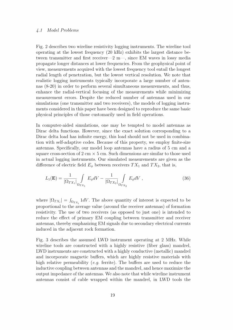
Fig. 2 describes two wireline resistivity logging instruments. The wireline tooloperating at the lowest frequency (20 kHz) exhibits the largest distance be-tween transmitter and first receiver—2 m—, since EM waves in lossy mediapropagate longer distances at lower frequencies. From the geophysical point ofview, measurements acquired with the lowest frequency tool entail the longestradial length of penetration, but the lowest vertical resolution. We note thatrealistic logging instruments typically incorporate a large number of anten-nas (8-20) in order to perform several simultaneous measurements, and thus,enhance the radial-vertical focusing of the measurements while minimizingmeasurement errors. Despite the reduced number of antennas used in oursimulations (one transmitter and two receivers), the models of logging instru-ments considered in this paper have been designed to reproduce the same basicphysical principles of those customarily used in field operations.

In computer-aided simulations, one may be tempted to model antennas asDirac delta functions. However, since the exact solution corresponding to aDirac delta load has infinite energy, this load should not be used in combina-tion with self-adaptive codes. Because of this property, we employ finite-sizeantennas. Specifically, our model loop antennas have a radius of 5 cm and asquare cross-section of 2 cm × 5 cm. Such dimensions are similar to those usedin actual logging instruments. Our simulated measurements are given as thedifference of electric field Eφ between receivers TX1 and TX2, that is,

L1(E) =1

|ΩTX1|

∫ΩTX1

EφdV − 1

|ΩTX2|

∫ΩTX2

EφdV , (36)

where |ΩTXi| =

∫ΩTXi

1dV . The above quantity of interest is expected to be

proportional to the average value (around the receiver antennas) of formationresistivity. The use of two receivers (as opposed to just one) is intended toreduce the effect of primary EM coupling between transmitter and receiverantennas, thereby emphasizing EM signals due to secondary electrical currentsinduced in the adjacent rock formation.

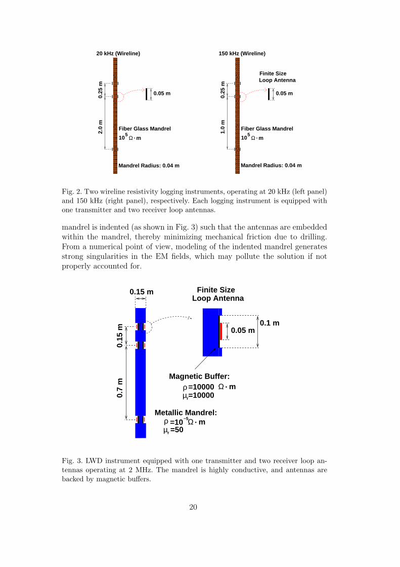
Fig. 3 describes the assumed LWD instrument operating at 2 MHz. Whilewireline tools are constructed with a highly resistive (fiber glass) mandrel,LWD instruments are constructed with a highly conductive (metallic) mandreland incorporate magnetic buffers, which are highly resistive materials withhigh relative permeability (e.g. ferrite). The buffers are used to reduce theinductive coupling between antennas and the mandrel, and hence maximize theoutput impedance of the antennas. We also note that while wireline instrumentantennas consist of cable wrapped within the mandrel, in LWD tools the

19

0.05 m

mΩ .

0.25

m

Fiber Glass Mandrel

Mandrel Radius: 0.04 m

1052.

0 m

20 kHz (Wireline)

0.05 m

mΩ .

0.25

m1.

0 m

150 kHz (Wireline)

Fiber Glass Mandrel

105

Finite SizeLoop Antenna

Mandrel Radius: 0.04 m

Fig. 2. Two wireline resistivity logging instruments, operating at 20 kHz (left panel)and 150 kHz (right panel), respectively. Each logging instrument is equipped withone transmitter and two receiver loop antennas.

mandrel is indented (as shown in Fig. 3) such that the antennas are embeddedwithin the mandrel, thereby minimizing mechanical friction due to drilling.From a numerical point of view, modeling of the indented mandrel generatesstrong singularities in the EM fields, which may pollute the solution if notproperly accounted for.

Ω . mµr

µr

Ω . m

0.15 m

0.05 m0.1 m

0.7

m

Magnetic Buffer:

=10000=10000ρ

Metallic Mandrel:ρ =10

−5

=50

Loop AntennaFinite Size

0.15

m

Fig. 3. LWD instrument equipped with one transmitter and two receiver loop an-tennas operating at 2 MHz. The mandrel is highly conductive, and antennas arebacked by magnetic buffers.

20

The three logging instruments described above are used to acquire measure-ments in the synthetic reservoir model described in Fig. 4. The formation iscomposed of seven different layers with varying resistivities, from 0.01 Ω· m to100 Ω· m. We consider a highly resistive oil-based mud in a possibly deviatedwell. We also include the effect of mud-filtrate radial invasion occurring inthree different porous and permeable sand layers.

mΩ .

mΩ .

mΩ .

mΩ .

mΩ .

mΩ .

mΩ .

mΩ .50

mΩ .20

mΩ .30O

il−Based Mud (1000 m

)

1.5 m

Ω

.

0.5 m0.65 m

3 m

SHALE

SHALE

3

200.05

0.1

100

1

1

4 m

SAND (WATER)

SAND (WATER)SAND (WATER)

SAND (WATER)

SAND (OIL)

Fig. 4. Deviated well penetrating a reservoir with various water- and oil-bearingsand layers.

4.2 Verification of Results and Convergence

This subsection is intended to verify our implementation of the new simulationmethod. We first observe that in a homogeneous, isotropic and unboundedformation all measurements should coincide independently of dip angle. Inparticular, regardless of dip angle, the exact solution should coincide with thatobtained for the axisymmetric case (vertical well). However, in the case of adeviated well we may need an infinite number of Fourier modes to reproducethe exact solution.

To verify the accuracy and reliability of our code, we first compute a high-accuracy approximation (below 0.01% relative error in the quantity of inter-est) of the exact solution for a vertical well. This high-accuracy solution iscomputed with a 2D hp-FE code, which has been extensively verified againstdifferent numerical methods [17,5,6] and analytical solutions [33]. Using this

21

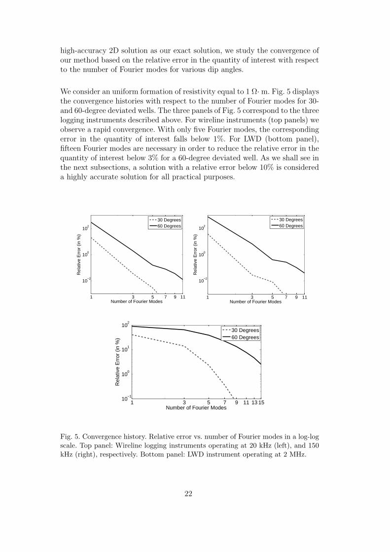
high-accuracy 2D solution as our exact solution, we study the convergence ofour method based on the relative error in the quantity of interest with respectto the number of Fourier modes for various dip angles.

We consider an uniform formation of resistivity equal to 1 Ω· m. Fig. 5 displaysthe convergence histories with respect to the number of Fourier modes for 30-and 60-degree deviated wells. The three panels of Fig. 5 correspond to the threelogging instruments described above. For wireline instruments (top panels) weobserve a rapid convergence. With only five Fourier modes, the correspondingerror in the quantity of interest falls below 1%. For LWD (bottom panel),fifteen Fourier modes are necessary in order to reduce the relative error in thequantity of interest below 3% for a 60-degree deviated well. As we shall see inthe next subsections, a solution with a relative error below 10% is considereda highly accurate solution for all practical purposes.

1 3 5 7 9 11

10−2

100

102

Number of Fourier Modes

Rel

ativ

e E

rror

(in

%)

30 Degrees60 Degrees

1 3 5 7 9 11

10−2

100

102

Number of Fourier Modes

Rel

ativ

e E

rror

(in

%)

30 Degrees60 Degrees

1 3 5 7 9 11 13 1510

−1

100

101

102

Number of Fourier Modes

Rel

ativ

e E

rror

(in

%)

30 Degrees60 Degrees

Fig. 5. Convergence history. Relative error vs. number of Fourier modes in a log-logscale. Top panel: Wireline logging instruments operating at 20 kHz (left), and 150kHz (right), respectively. Bottom panel: LWD instrument operating at 2 MHz.

22

4.3 Performance and Error Analysis

In this subsection, we consider the wireline logging instrument operating at 150kHz in conjunction with the model formation shown in Fig. 4 and study theconvergence properties of the numerical solution as a function of the numberof Fourier modes used in the calculations.

For a fixed number of Fourier modes in the quasi-azimuthal direction, the hp-FE strategy automatically generates an optimal grid that delivers an error inthe quantity of interest below a given tolerance error. In our case, we selecta tolerance error equal to 1%. However, the total error may be considerablylarger, since the number of Fourier modes is fixed. Fig. 6 displays the finalresults (as we move the logging instrument along the well trajectory) for 1,3, 5, 7, and 9 Fourier modes. When using 3 Fourier modes, the total error isbelow 5% (see Fig. 6, bottom-right panel), which indicates that the solution ishighly accurate for our purposes. As a matter of fact, it is (almost) impossibleto observe a difference between the results obtained with 3, 5, 7, or 9 Fouriermodes (see Fig. 6, top panels).

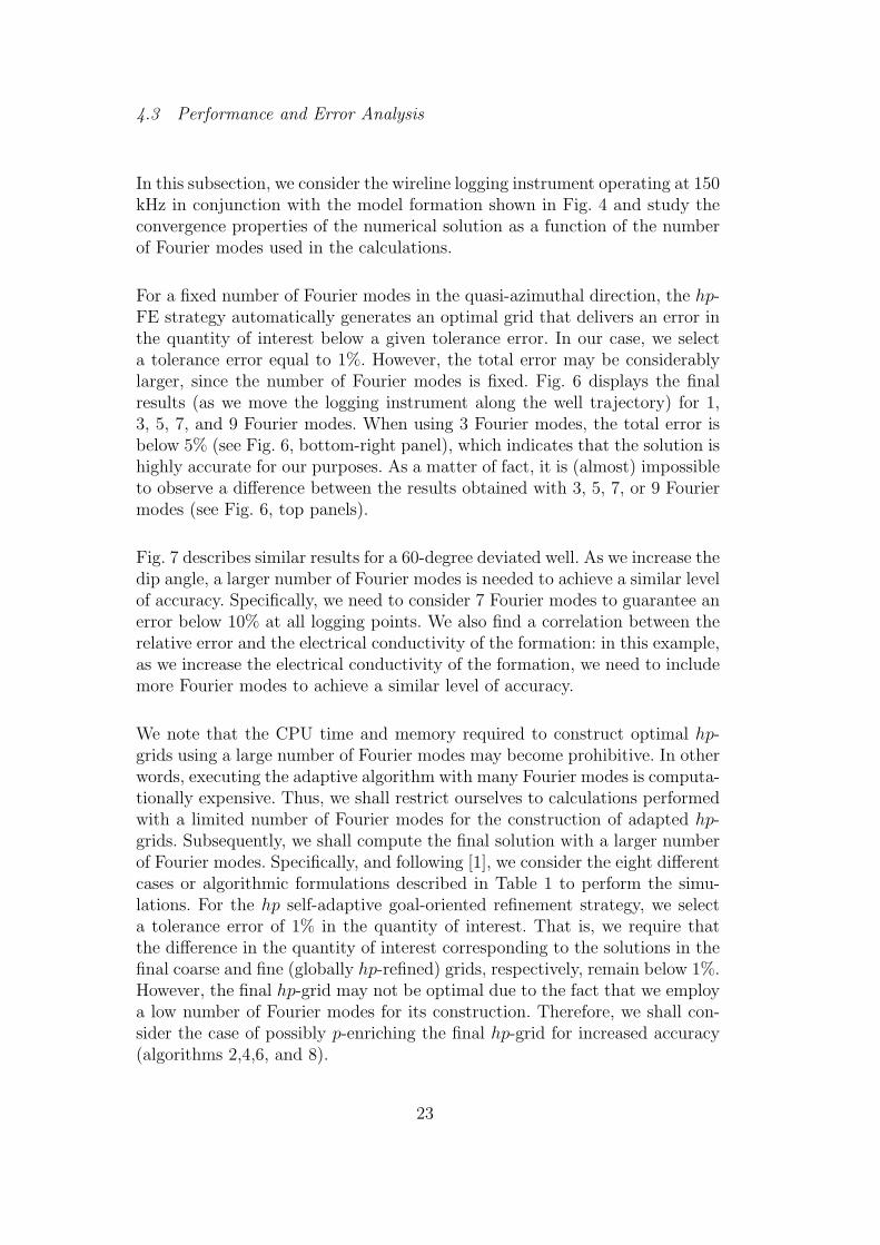
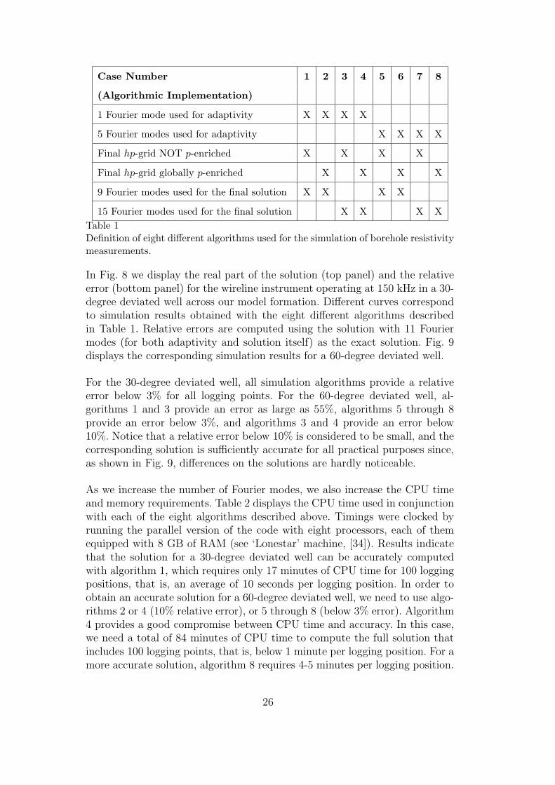
Fig. 7 describes similar results for a 60-degree deviated well. As we increase thedip angle, a larger number of Fourier modes is needed to achieve a similar levelof accuracy. Specifically, we need to consider 7 Fourier modes to guarantee anerror below 10% at all logging points. We also find a correlation between therelative error and the electrical conductivity of the formation: in this example,as we increase the electrical conductivity of the formation, we need to includemore Fourier modes to achieve a similar level of accuracy.

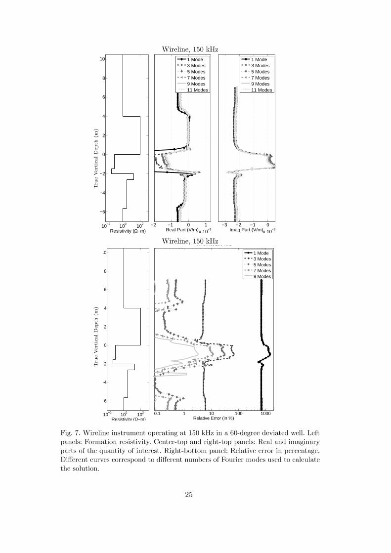
We note that the CPU time and memory required to construct optimal hp-grids using a large number of Fourier modes may become prohibitive. In otherwords, executing the adaptive algorithm with many Fourier modes is computa-tionally expensive. Thus, we shall restrict ourselves to calculations performedwith a limited number of Fourier modes for the construction of adapted hp-grids. Subsequently, we shall compute the final solution with a larger numberof Fourier modes. Specifically, and following [1], we consider the eight differentcases or algorithmic formulations described in Table 1 to perform the simu-lations. For the hp self-adaptive goal-oriented refinement strategy, we selecta tolerance error of 1% in the quantity of interest. That is, we require thatthe difference in the quantity of interest corresponding to the solutions in thefinal coarse and fine (globally hp-refined) grids, respectively, remain below 1%.However, the final hp-grid may not be optimal due to the fact that we employa low number of Fourier modes for its construction. Therefore, we shall con-sider the case of possibly p-enriching the final hp-grid for increased accuracy(algorithms 2,4,6, and 8).

23

Wireline, 150 kHz

10−2

100

102

−6

−4

−2

0

2

4

6

8

10

Resistivity (Ω−m)−2 −1 0 1

x 10−3

Wireline, 150 Khz

Real Part (V/m)

−3 −2 −1 0x 10

−3Imag Part (V/m)

1 Mode3 Modes5 Modes7 Modes9 Modes

1 Mode3 Modes5 Modes7 Modes9 Modes

Wireline, 150 kHz

10−2

100

102

−6

−4

−2

0

2

4

6

8

10

Resistivity (Ω−m)0.01 0.1 1 10 100

Wireline, 150 Khz

Relative Error (in %)

1 Mode3 Modes5 Modes7 Modes

Tru

eVer

tica

lD

epth

(m)

Tru

eVer

tica

lD

epth

(m)

Fig. 6. Wireline instrument operating at 150 kHz in a 30-degree deviated well. Leftpanels: Formation resistivity. Center-top and right-top panels: Real and imaginaryparts of the quantity of interest. Right-bottom panel: Relative error in percentage.Different curves correspond to different numbers of Fourier modes used to calculatethe solution.

24

Wireline, 150 kHz

10−2

100

102

−6

−4

−2

0

2

4

6

8

10

Resistivity (Ω−m)−2 −1 0 1

x 10−3

Wireline, 150 Khz

Real Part (V/m)

−3 −2 −1 0x 10

−3Imag Part (V/m)

1 Mode3 Modes5 Modes7 Modes9 Modes11 Modes

1 Mode3 Modes5 Modes7 Modes9 Modes11 Modes

Wireline, 150 kHz

10−2

100

102

−6

−4

−2

0

2

4

6

8

10

Resistivity (Ω−m)0.1 1 10 100 1000

Wireline, 150 Khz

Relative Error (in %)

1 Mode3 Modes5 Modes7 Modes9 Modes

Tru

eVer

tica

lD

epth

(m)

Tru

eVer

tica

lD

epth

(m)

Fig. 7. Wireline instrument operating at 150 kHz in a 60-degree deviated well. Leftpanels: Formation resistivity. Center-top and right-top panels: Real and imaginaryparts of the quantity of interest. Right-bottom panel: Relative error in percentage.Different curves correspond to different numbers of Fourier modes used to calculatethe solution.

25

Case Number 1 2 3 4 5 6 7 8

(Algorithmic Implementation)

1 Fourier mode used for adaptivity X X X X

5 Fourier modes used for adaptivity X X X X

Final hp-grid NOT p-enriched X X X X

Final hp-grid globally p-enriched X X X X

9 Fourier modes used for the final solution X X X X

15 Fourier modes used for the final solution X X X XTable 1Definition of eight different algorithms used for the simulation of borehole resistivitymeasurements.

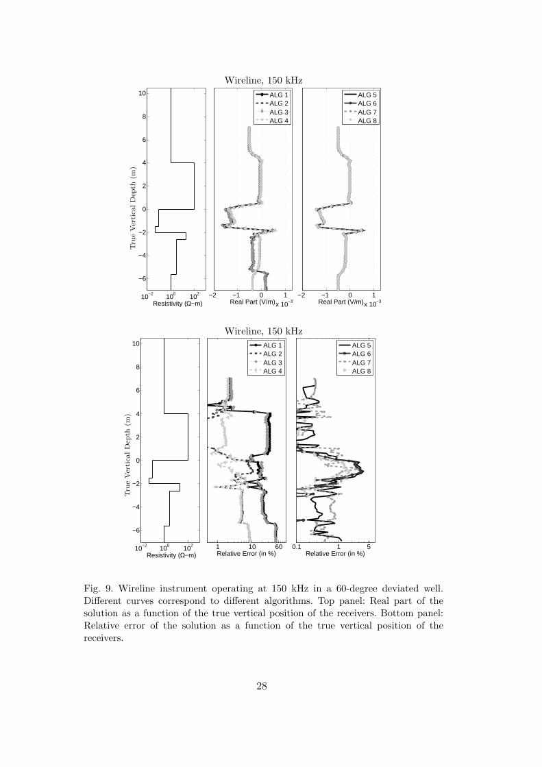
In Fig. 8 we display the real part of the solution (top panel) and the relativeerror (bottom panel) for the wireline instrument operating at 150 kHz in a 30-degree deviated well across our model formation. Different curves correspondto simulation results obtained with the eight different algorithms describedin Table 1. Relative errors are computed using the solution with 11 Fouriermodes (for both adaptivity and solution itself) as the exact solution. Fig. 9displays the corresponding simulation results for a 60-degree deviated well.

For the 30-degree deviated well, all simulation algorithms provide a relativeerror below 3% for all logging points. For the 60-degree deviated well, al-gorithms 1 and 3 provide an error as large as 55%, algorithms 5 through 8provide an error below 3%, and algorithms 3 and 4 provide an error below10%. Notice that a relative error below 10% is considered to be small, and thecorresponding solution is sufficiently accurate for all practical purposes since,as shown in Fig. 9, differences on the solutions are hardly noticeable.

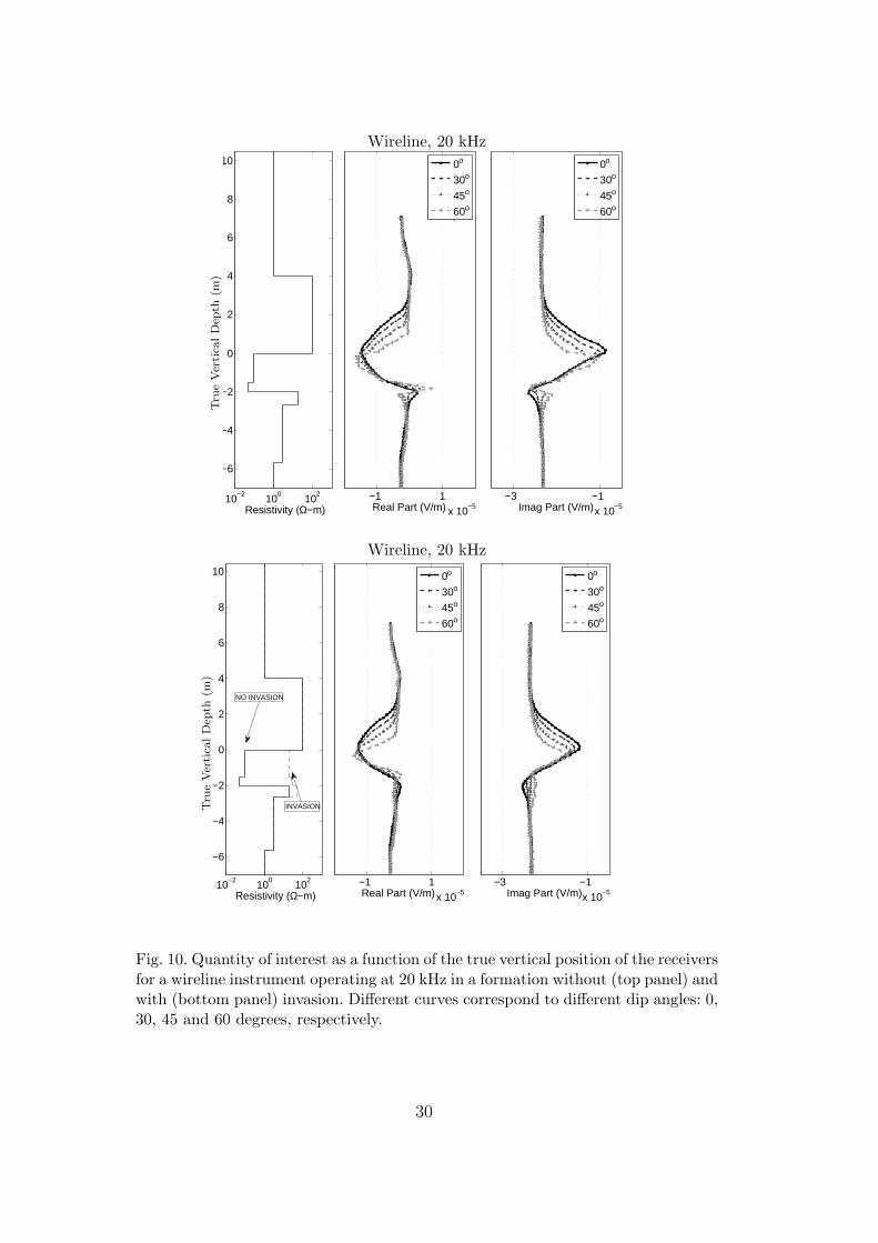
As we increase the number of Fourier modes, we also increase the CPU timeand memory requirements. Table 2 displays the CPU time used in conjunctionwith each of the eight algorithms described above. Timings were clocked byrunning the parallel version of the code with eight processors, each of themequipped with 8 GB of RAM (see ‘Lonestar’ machine, [34]). Results indicatethat the solution for a 30-degree deviated well can be accurately computedwith algorithm 1, which requires only 17 minutes of CPU time for 100 loggingpositions, that is, an average of 10 seconds per logging position. In order toobtain an accurate solution for a 60-degree deviated well, we need to use algo-rithms 2 or 4 (10% relative error), or 5 through 8 (below 3% error). Algorithm4 provides a good compromise between CPU time and accuracy. In this case,we need a total of 84 minutes of CPU time to compute the full solution thatincludes 100 logging points, that is, below 1 minute per logging position. For amore accurate solution, algorithm 8 requires 4-5 minutes per logging position.

26

Wireline, 150 kHz

10−2

100

102

−6

−4

−2

0

2

4

6

8

10

Resistivity (Ω−m)−2 −1 0 1

x 10−3

Wireline, 150 Khz

Real Part (V/m)

−2 −1 0 1x 10

−3Real Part (V/m)

ALG 1ALG 2ALG 3ALG 4

ALG 5ALG 6ALG 7ALG 8

Wireline, 150 kHz

10−2

100

102

−6

−4

−2

0

2

4

6

8

10

Resistivity (Ω−m)0.1 1 3

Wireline, 150 Khz

Relative Error (in %)

0.1 1Relative Error (in %)

ALG 1ALG 2ALG 3ALG 4

ALG 5ALG 6ALG 7ALG 8

Tru

eVer

tica

lD

epth

(m)

Tru

eVer

tica

lD

epth

(m)

Fig. 8. Wireline instrument operating at 150 kHz in a 30-degree deviated well.Different curves correspond to different algorithms. Top panel: Real part of thesolution as a function of the true vertical position of the receivers. Bottom panel:Relative error of the solution as a function of the true vertical position of thereceivers.

27

Wireline, 150 kHz

10−2

100

102

−6

−4

−2

0

2

4

6

8

10

Resistivity (Ω−m)−2 −1 0 1

x 10−3

Wireline, 150 Khz

Real Part (V/m)

−2 −1 0 1x 10

−3Real Part (V/m)

ALG 1ALG 2ALG 3ALG 4

ALG 5ALG 6ALG 7ALG 8

Wireline, 150 kHz

10−2

100

102

−6

−4

−2

0

2

4

6

8

10

Resistivity (Ω−m)1 10 60

Wireline, 150 Khz

Relative Error (in %)

0.1 1 5Relative Error (in %)

ALG 1ALG 2ALG 3ALG 4

ALG 5ALG 6ALG 7ALG 8

Tru

eVer

tica

lD

epth

(m)

Tru

eVer

tica

lD

epth

(m)

Fig. 9. Wireline instrument operating at 150 kHz in a 60-degree deviated well.Different curves correspond to different algorithms. Top panel: Real part of thesolution as a function of the true vertical position of the receivers. Bottom panel:Relative error of the solution as a function of the true vertical position of thereceivers.

28

Algorithmic Implementation 1 2 3 4 5 6 7 8

CPU Time (Minutes) 17’ 49’ 36’ 131’ 144’ 188’ 173’ 269’

30-Degree Deviated

CPU Time (Minutes) 12’ 31’ 22’ 84’ 263’ 381’ 312’ 442’

60-Degree DeviatedTable 2CPU simulation time required for the simulation of 100 logging positions as a func-tion of the algorithm (case number) for the wireline instrument operating at 150kHz in the model formation shown in Fig. 4. The two rows of results correspond to30- and 60-degree deviated wells, respectively.

4.4 Numerical Applications

In this subsection, we consider the three logging instruments described aboveand the model formation shown in Fig. 4, and compare results obtained with0-, 30-, 45-, and 60-degree deviated wells. We also analyze the effect of mudinvasion on the simulated measurements.

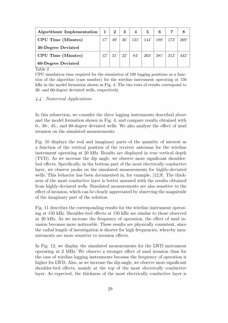
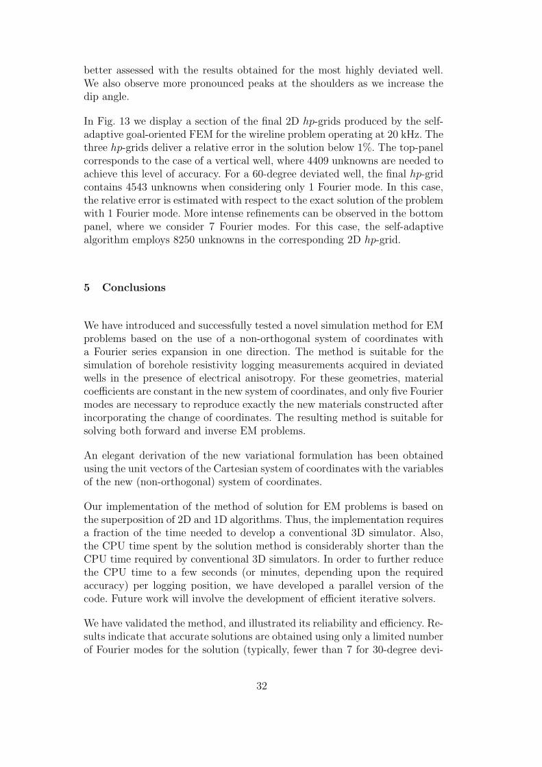
Fig. 10 displays the real and imaginary parts of the quantity of interest asa function of the vertical position of the receiver antennas for the wirelineinstrument operating at 20 kHz. Results are displayed in true vertical depth(TVD). As we increase the dip angle, we observe more significant shoulder-bed effects. Specifically, in the bottom part of the most electrically conductivelayer, we observe peaks on the simulated measurements for highly-deviatedwells. This behavior has been documented in, for example, [12,9]. The thick-ness of the most conductive layer is better assessed with the results obtainedfrom highly-deviated wells. Simulated measurements are also sensitive to theeffect of invasion, which can be clearly appreciated by observing the magnitudeof the imaginary part of the solution.

Fig. 11 describes the corresponding results for the wireline instrument operat-ing at 150 kHz. Shoulder-bed effects at 150 kHz are similar to those observedat 20 kHz. As we increase the frequency of operation, the effect of mud in-vasion becomes more noticeable. These results are physically consistent, sincethe radial length of investigation is shorter for high frequencies, whereby mea-surements are more sensitive to invasion effects.

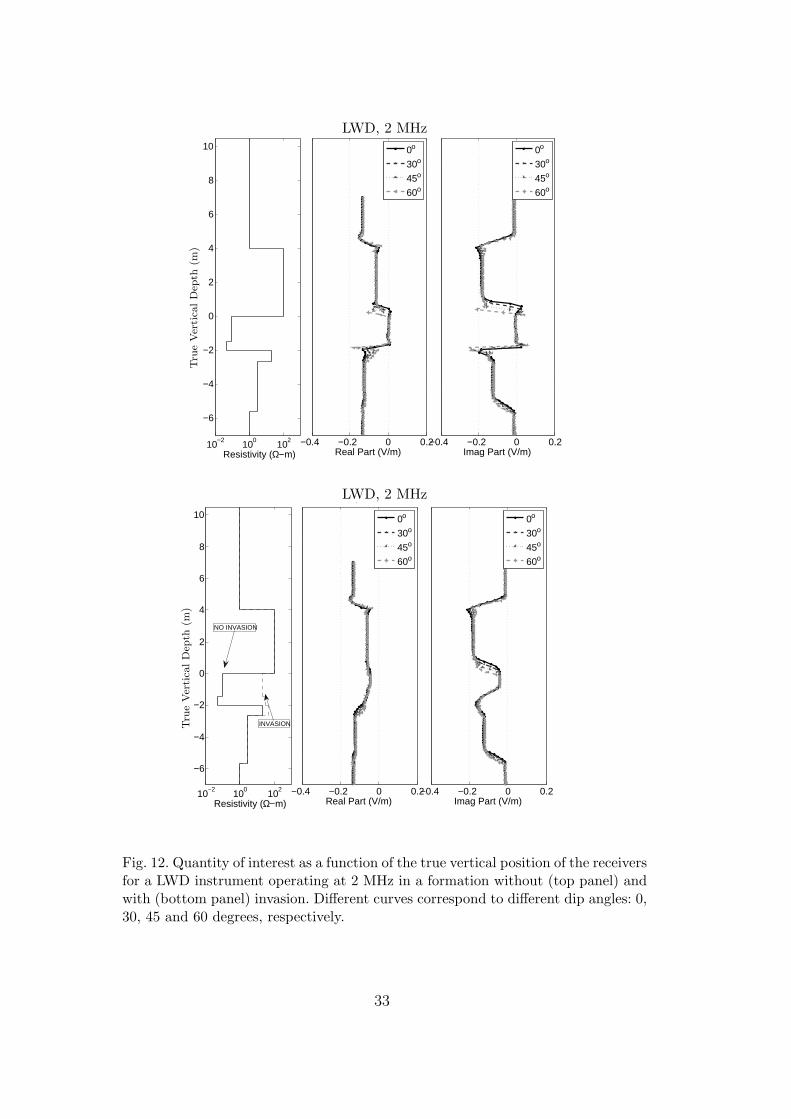
In Fig. 12, we display the simulated measurements for the LWD instrumentoperating at 2 MHz. We observe a stronger effect of mud invasion than forthe case of wireline logging instruments because the frequency of operation ishigher for LWD. Also, as we increase the dip angle, we observe more significantshoulder-bed effects, mainly at the top of the most electrically conductivelayer. As expected, the thickness of the most electrically conductive layer is

29

Wireline, 20 kHz

10−2

100

102

−6

−4

−2

0

2

4

6

8

10

Resistivity (Ω−m)−1 1

x 10−5

Wireline, 20 Khz.

Real Part (V/m)

−3 −1x 10

−5Imag Part (V/m)

0o

30o

45o

60o

0o

30o

45o

60o

Wireline, 20 kHz

10−2

100

102

−6

−4

−2

0

2

4

6

8

10

Resistivity (Ω−m)−1 1

x 10−5

Wireline, 20 Khz.

Real Part (V/m)

−3 −1x 10

−5Imag Part (V/m)

0o

30o

45o

60o

0o

30o

45o

60o

INVASION

NO INVASION

Tru

eVer

tica

lD

epth

(m)

Tru

eVer

tica

lD

epth

(m)

Fig. 10. Quantity of interest as a function of the true vertical position of the receiversfor a wireline instrument operating at 20 kHz in a formation without (top panel) andwith (bottom panel) invasion. Different curves correspond to different dip angles: 0,30, 45 and 60 degrees, respectively.

30

Wireline, 150 kHz

10−2

100

102

−6

−4

−2

0

2

4

6

8

10

Resistivity (Ω−m)−2 −1 0 1

x 10−3

Wireline, 150 Khz

Real Part (V/m)

−3 −2 −1 0x 10

−3Imag Part (V/m)

0o

30o

45o

60o

0o

30o

45o

60o

Wireline, 150 kHz

10−2

100

102

−6

−4

−2

0

2

4

6

8

10

Resistivity (Ω−m)−2 −1 0 1

x 10−3

Wireline, 150 Khz

Real Part (V/m)

−3 −2 −1 0x 10

−3Imag Part (V/m)

0o

30o

45o

60o

0o

30o

45o

60o

INVASION

NO INVASION

Tru

eVer

tica

lD

epth

(m)

Tru

eVer

tica

lD

epth

(m)

Fig. 11. Quantity of interest as a function of the true vertical position of the re-ceivers for a wireline instrument operating at 150 kHz in a formation without (toppanel) and with (bottom panel) invasion. Different curves correspond to differentdip angles: 0, 30, 45 and 60 degrees, respectively.

31

better assessed with the results obtained for the most highly deviated well.We also observe more pronounced peaks at the shoulders as we increase thedip angle.

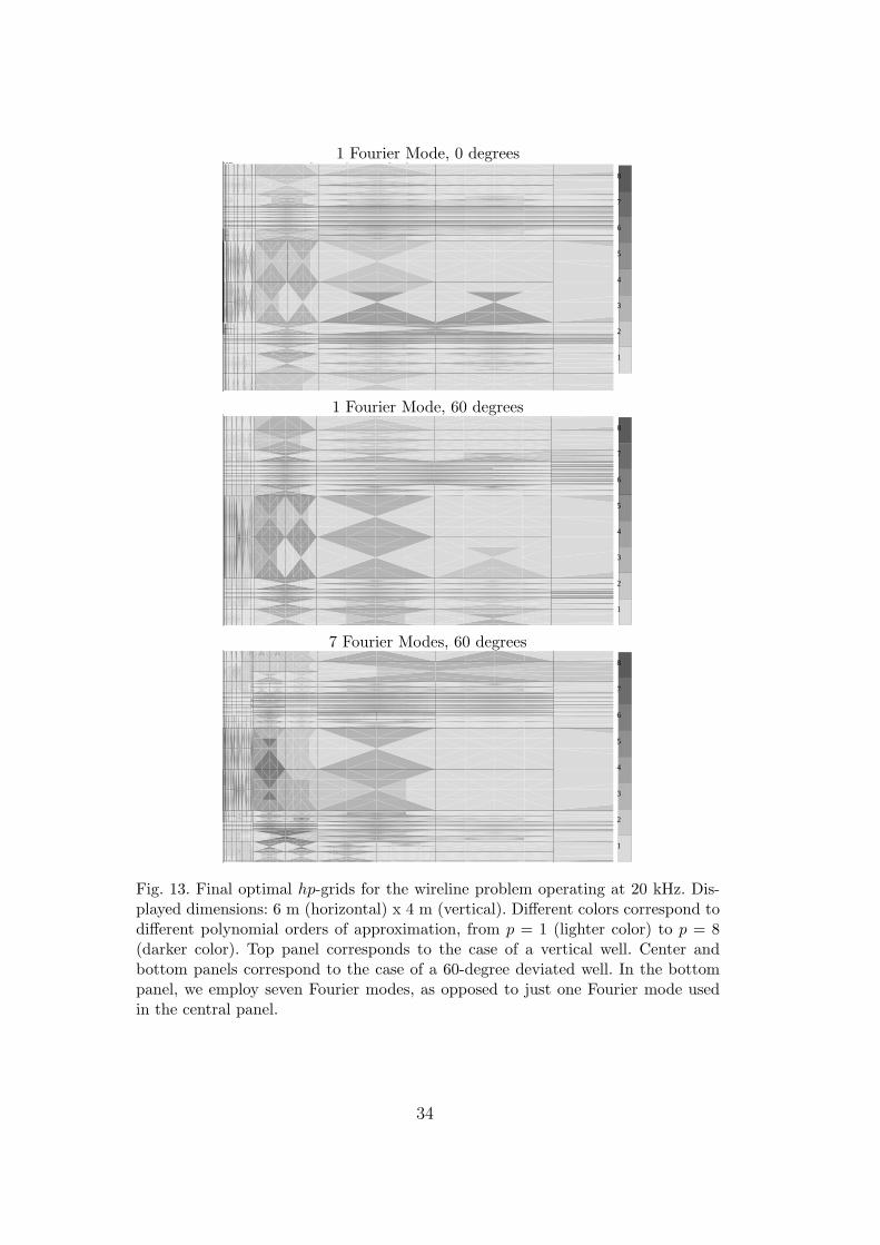
In Fig. 13 we display a section of the final 2D hp-grids produced by the self-adaptive goal-oriented FEM for the wireline problem operating at 20 kHz. Thethree hp-grids deliver a relative error in the solution below 1%. The top-panelcorresponds to the case of a vertical well, where 4409 unknowns are needed toachieve this level of accuracy. For a 60-degree deviated well, the final hp-gridcontains 4543 unknowns when considering only 1 Fourier mode. In this case,the relative error is estimated with respect to the exact solution of the problemwith 1 Fourier mode. More intense refinements can be observed in the bottompanel, where we consider 7 Fourier modes. For this case, the self-adaptivealgorithm employs 8250 unknowns in the corresponding 2D hp-grid.

5 Conclusions

We have introduced and successfully tested a novel simulation method for EMproblems based on the use of a non-orthogonal system of coordinates witha Fourier series expansion in one direction. The method is suitable for thesimulation of borehole resistivity logging measurements acquired in deviatedwells in the presence of electrical anisotropy. For these geometries, materialcoefficients are constant in the new system of coordinates, and only five Fouriermodes are necessary to reproduce exactly the new materials constructed afterincorporating the change of coordinates. The resulting method is suitable forsolving both forward and inverse EM problems.

An elegant derivation of the new variational formulation has been obtainedusing the unit vectors of the Cartesian system of coordinates with the variablesof the new (non-orthogonal) system of coordinates.

Our implementation of the method of solution for EM problems is based onthe superposition of 2D and 1D algorithms. Thus, the implementation requiresa fraction of the time needed to develop a conventional 3D simulator. Also,the CPU time spent by the solution method is considerably shorter than theCPU time required by conventional 3D simulators. In order to further reducethe CPU time to a few seconds (or minutes, depending upon the requiredaccuracy) per logging position, we have developed a parallel version of thecode. Future work will involve the development of efficient iterative solvers.

We have validated the method, and illustrated its reliability and efficiency. Re-sults indicate that accurate solutions are obtained using only a limited numberof Fourier modes for the solution (typically, fewer than 7 for 30-degree devi-

32

LWD, 2 MHz

10−2

100

102

−6

−4

−2

0

2

4

6

8

10

Resistivity (Ω−m)−0.4 −0.2 0 0.2

LWD, 2 Mhz

Real Part (V/m)

−0.4 −0.2 0 0.2Imag Part (V/m)

0o

30o

45o

60o

0o

30o

45o

60o

LWD, 2 MHz

10−2

100

102

−6

−4

−2

0

2

4

6

8

10

Resistivity (Ω−m)−0.4 −0.2 0 0.2

LWD, 2 Mhz

Real Part (V/m)

−0.4 −0.2 0 0.2Imag Part (V/m)

0o

30o

45o

60o

0o

30o

45o

60o

INVASION

NO INVASION

Tru

eVer

tica

lD

epth

(m)

Tru

eVer

tica

lD

epth

(m)

Fig. 12. Quantity of interest as a function of the true vertical position of the receiversfor a LWD instrument operating at 2 MHz in a formation without (top panel) andwith (bottom panel) invasion. Different curves correspond to different dip angles: 0,30, 45 and 60 degrees, respectively.

33

1 Fourier Mode, 0 degrees

1

2

3

4

5

6

7

8

-0.2444444 6.940741 -1.229630

3.214815 2Dhp90: A Fully automatic hp-adaptive Finite Element code

1 Fourier Mode, 60 degrees

1

2

3

4

5

6

7

8

-0.2148148 6.970370 0.8296296

5.274074 2Dhp90: A Fully automatic hp-adaptive Finite Element code

7 Fourier Modes, 60 degrees

1

2

3

4

5

6

7

8

-0.2666667 6.918519 0.7629629

5.207407 2Dhp90: A Fully automatic hp-adaptive Finite Element code

Fig. 13. Final optimal hp-grids for the wireline problem operating at 20 kHz. Dis-played dimensions: 6 m (horizontal) x 4 m (vertical). Different colors correspond todifferent polynomial orders of approximation, from p = 1 (lighter color) to p = 8(darker color). Top panel corresponds to the case of a vertical well. Center andbottom panels correspond to the case of a 60-degree deviated well. In the bottompanel, we employ seven Fourier modes, as opposed to just one Fourier mode usedin the central panel.

34

ated wells, and fewer than 13 for 60-degree deviated wells), thereby enablinga significant reduction of computer complexity.

From the physical point of view, simulated measurements indicate a highersensitive to mud-filtrate invasion in electrical conductive layers. In addition,we observe significant shoulder-bed effects on highly deviated wells. Thus, themethod provides precise quantitative results, and enables the computer-aidedstudy of common effects occurring in well-logging applications such as theinvasion of mud filtrate into permeable formations.

Future work will involve: (1) the development of an iterative solver usinga block-Jacobi preconditioner with the blocks defined by all trial and testfunctions associated with a single Fourier mode (that is, a 2D problem), and(2) implementation of a self-adaptive scheme for the Fourier modes. Thesefeatures will further decrease the computational requirements needed to solvepractical applications, and will enable the use of an optimal number of Fouriermodes for each FE.

ACKNOWLEDGMENTS

The work presented in this paper was supported by The University of Texas atAustin’s Joint Industry Research Consortium on Formation Evaluation spon-sored by Anadarko, Aramco, Baker Atlas, British Gas, BHP-Billiton, BP,Chevron, Conoco-Phillips, ENI E&P, ExxonMobil, Halliburton, Marathon,Mexican Institute for Petroleum, Hydro, Occidental Petroleum, Petrobras,Schlumberger, Shell E&P, Statoil, TOTAL, and Weatherford International,Ltd.

The work of the fourth author has been partially supported by the Foundationfor Polish Science under Homming Programme.

The authors acknowledge the Texas Advanced Computing Center (TACC) atThe University of Texas at Austin for providing high performance computingresources that have contributed to the research results reported in this paper.

References

[1] D. Pardo, V. M. Calo, C. Torres-Verdin, M. J. Nam, Fourier series expansionin a non-orthogonal system of coordinates for simulation of 3D DC boreholeresistivity measurements, In press at: Computer Methods in Applied Mechanicsand Engineering, doi:10.1016/j.cma.2007.12.003.

35

[2] B. Heinrich, The fourier-finite-element method for Poisson’s equation inaxisymmetric domains with edges, SIAM Journal on Numerical Analysis 33 (5)(1996) 1885–1911.

[3] C. Bernardi, M. Dauge, Y. Maday, Spectral Methods for AxisymmetricDomains, ELSEVIER, 1999.

[4] X. Lu, D. L. Alumbaugh, One-dimensional inversion of three-componentinduction logging in anisotropic media, SEG Expanded Abstract 20 (2001) 376–380.

[5] D. Pardo, L. Demkowicz, C. Torres-Verdin, M. Paszynski, Simulation ofresistivity logging-while-drilling (LWD) measurements using a self-adaptivegoal-oriented hp-finite element method, SIAM Journal on Applied Mathematics66 (2006) 2085–2106.

[6] D. Pardo, C. Torres-Verdin, L. Demkowicz, Simulation of multi-frequencyborehole resistivity measurements through metal casing using a goal-orientedhp-finite element method, IEEE Transactions on Geosciences and RemoteSensing 44 (2006) 2125–2135.

[7] D. Pardo, C. Torres-Verdin, L. Demkowicz, Feasibility study for two-dimensional frequency dependent electromagnetic sensing through casing,Geophysics 72 (2007) F111–F118.

[8] J. Zhang, R. L. Mackie, T. R. Madden, 3-D resistivity forward modeling andinversion using conjugate gradients, Geophysics 60 (1995) 1312–1325.

[9] V. L. Druskin, L. A. Knizhnerman, P. Lee, New spectral Lanczos decompositionmethod for induction modeling in arbitrary 3-D geometry, Geophysics 64 (3)(1999) 701–706.

[10] G. A. Newman, D. L. Alumbaugh, Three-dimensional induction loggingproblems, part 2: A finite-difference solution, Geophysics 67 (2) (2002) 484–491.

[11] S. Davydycheva, V. Druskin, T. Habashy, An efficient finite-difference schemefor electromagnetic logging in 3D anisotropic inhomogeneous media, Geophysics68 (5) (2003) 1525–1536.

[12] T. Wang, S. Fang, 3-D electromagnetic anisotropy modeling using finitedifferences, Geophysics 66 (5) (2001) 1386–1398.

[13] T. Wang, J. Signorelli, Finite-difference modeling of electromagnetic toolresponse for logging while drilling, Geophysics 69 (1) (2004) 152–160.

[14] D. B. Avdeev, A. V. Kuvshinov, O. V. Pankratov, G. A. Newman, Three-dimensional induction logging problems, part 1: An integral equation solutionand model comparisons, Geophysics 67 (2002) 413–426.

[15] D. Pardo, C. Torres-Verdin, M. Paszynski, Simulation of 3D DC boreholeresistivity measurements with a goal-oriented hp finite element method. Part II:Through casing resistivity instruments, Computational Geosciences, in press.Preprint available at: www.ices.utexas.edu/%7Epardo.

36

[16] R. F. Harrington, Time-Harmonic Electromagnetic Fields, McGraw-Hill, NewYork, 1961.

[17] D. Pardo, L. Demkowicz, C. Torres-Verdin, M. Paszynski, A goal oriented hp-adaptive finite element strategy with electromagnetic applications. Part II:electrodynamics, Computer Methods in Applied Mechanics and Engineering.196 (2007) 3585–3597.

[18] I. Gomez-Revuelto, L. Garcia-Castillo, L. Demkowicz, A comparison betweenseveral mesh truncation methods for hp-adaptivity in electromagnetics, in:(ICEAA07), Torino (Italia), 2007, invited paper to the Special Session“Numerical Methods for Solving Maxwell Equations in the Frequency Domain”.

[19] W. Cecot, W. Rachowicz, L. Demkowicz, An hp-adaptive finite element methodfor electromagnetics. III: A three-dimensional infinite element for Maxwell’sequations, International Journal of Numerical Methods in Engineering 57 (7)(2003) 899–921.

[20] D. Pardo, L. Demkowicz, C. Torres-Verdin, C. Michler, PML enhanced witha self-adaptive goal-oriented hp finite-element method and applications tothrough-casing borehole resistivity measurements, Submitted to: SIAM Journalon Scientific Computing. Preprint available at: www.ices.utexas.edu/%7Epardo.

[21] I. Gomez-Revuelto, L. E. Garcia-Castillo, D. Pardo, L. Demkowicz, A two-dimensional self-adaptive hp finite element method for the analysis of openregion problems in electromagnetics, IEEE Transactions on Magnetics 43 (4)(2007) 1337–1340.

[22] L. Demkowicz, Computing with hp-Adaptive Finite Elements. Volume I: Oneand Two Dimensional Elliptic and Maxwell Problems, Chapman and Hall, 2006.

[23] A. Ward, J. B. Pendry, Calculating photonic Green’s functions using anonorthogonal finite-difference time-domain method, Phys. Rev. B 58 (1998)7252–9.

[24] W. C. Chew, W. H. Weedon, A 3D perfectly matched medium from modifiedMaxwell’s equations with streched coordinates, Microwave Opt. Tech. Lett. 7(1994) 599–604.

[25] F. L. Teixeira, W. C. Chew, PML-FDTD in cylindrical and spherical grid, IEEEMicrowave Guided Wave Lett. 7 (1997) 285–287.

[26] L. Demkowicz, Finite element methods for Maxwell equations, Encyclopedia ofComputational Mechanics, (eds. E. Stein, R. de Borst, T.J.R. Hughes), Wileyand Sons 1 (26).

[27] D. N. Arnold, R. S. Falk, R. Winther, Multigrid in H(div) and H(curl), Numer.Math. 85 (2) (2000) 197–217.

[28] R. Hiptmair, Multigrid method for Maxwell’s equations, SIAM J. Numer. Anal.36 (1) (1998) 204–225.

37

[29] P. R. Amestoy, I. S. Duff, J.-Y. L’Excellent, Multifrontal parallel distributedsymmetric and unsymmetric solvers, Computer Methods in Applied Mechanicsand Engineering 184 (2000) 501–520.

[30] P. R. Amestoy, I. S. Duff, J. Koster, J.-Y. L’Excellent, A fully asynchronousmultifrontal solver using distributed dynamic scheduling, SIAM Journal ofMatrix Analysis and Applications 23 (1) (2001) 15–41.

[31] P. R. Amestoy, A. Guermouche, J.-Y. L’Excellent, S. Pralet, Hybrid schedulingfor the parallel solution of linear systems, Parallel Computing 32 (2006) 136–156.

[32] www-users.cs.umn.edu/ karypis/metis, METIS - Family of MultilevelPartitioning Algorithms (2007).

[33] M. Paszynski, L. Demkowicz, D. Pardo, Verification of goal-oriented hp-adaptivity, Computers and Mathematics with Applications 50 (2005) 1395–1404.

[34] http://www.tacc.utexas.edu, TACC - Texas Advanced Computing Center(2007).

38