Fourier Series and TransformKEEE343 Communication Theory

Lecture #8, March 29, 2011Prof. Young-Chai Kokoyc@korea.ac.kr

Review

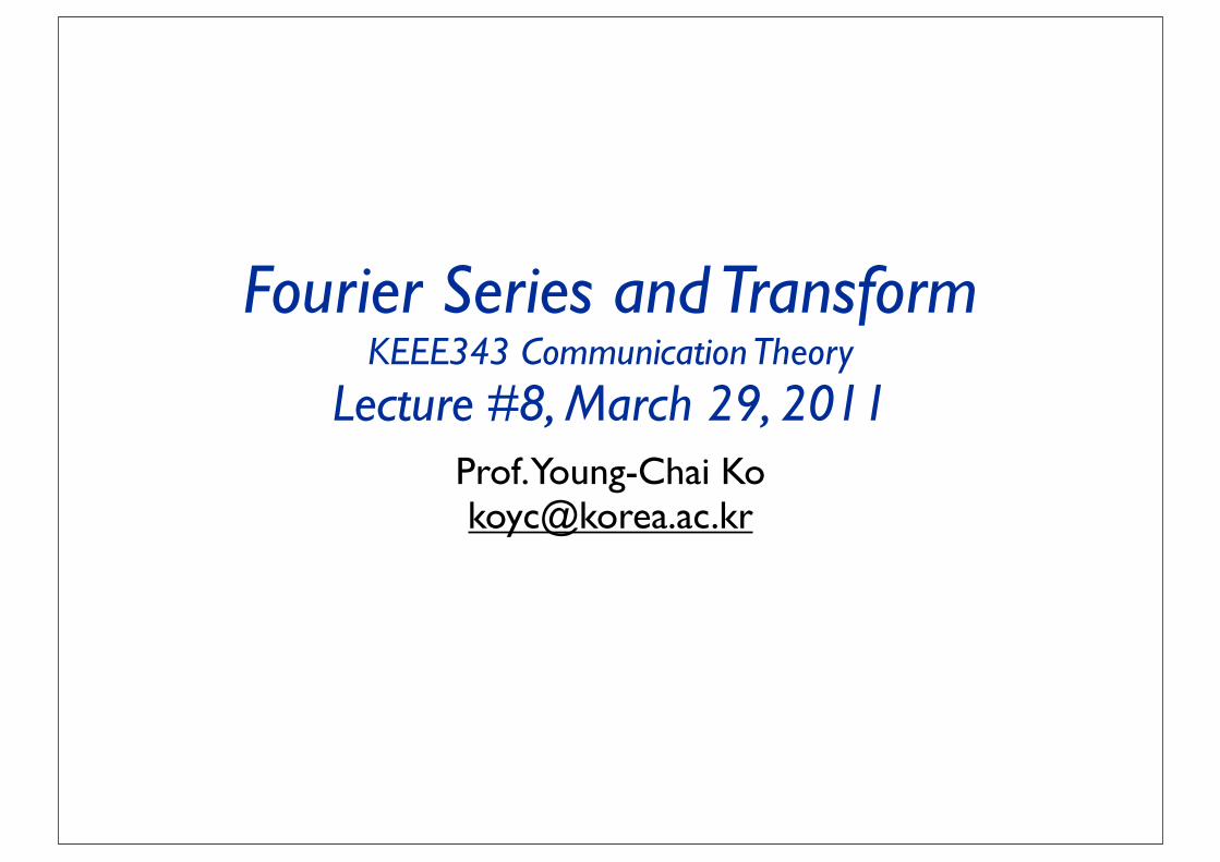
• Properties of Fourier Transform

• Time shift, frequency shift, modulation properties

• Energy theorem

• Inverse relation between time and frequency

• Bandwidth

• Dirac delta function

• Gaussian pulse

Summary

·•Fourier transform

·•Fourier transform of special function (Sec. 2.4)

·•Delta function

·•Signum function

·•Unit step function

·•Fourier transform of periodic signals (Sec. 2.5)

·•Transmission of signals through linear systems: Convolution revisited (Sec. 2.6)

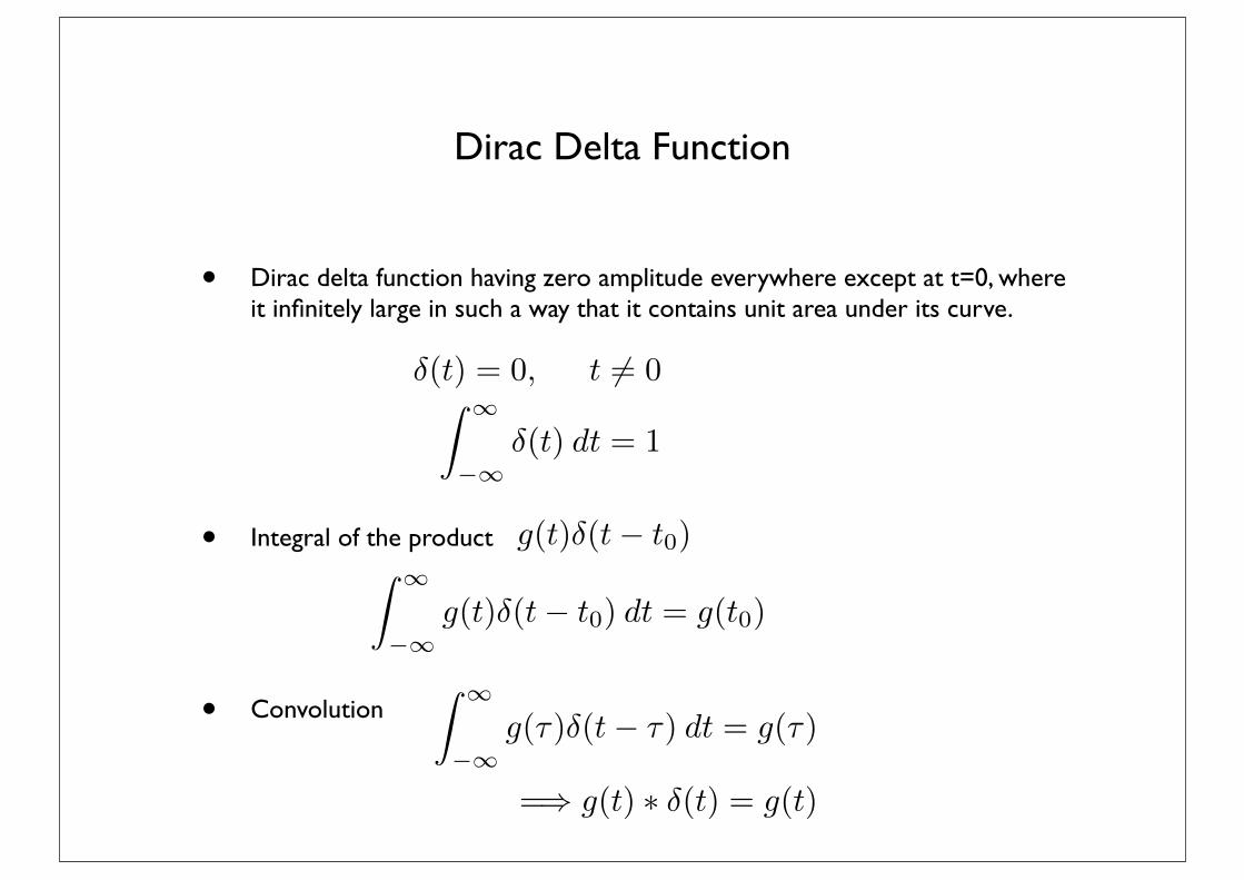
Dirac Delta Function

• Dirac delta function having zero amplitude everywhere except at t=0, where it infinitely large in such a way that it contains unit area under its curve.

• Integral of the product

• Convolution

�(t) = 0, t 6= 0Z 1

�1�(t) dt = 1

g(t)�(t� t0)Z 1

�1g(t)�(t� t0) dt = g(t0)

Z 1

�1g(⇥)�(t� ⇥) dt = g(⇥)

=) g(t) ⇤ �(t) = g(t)

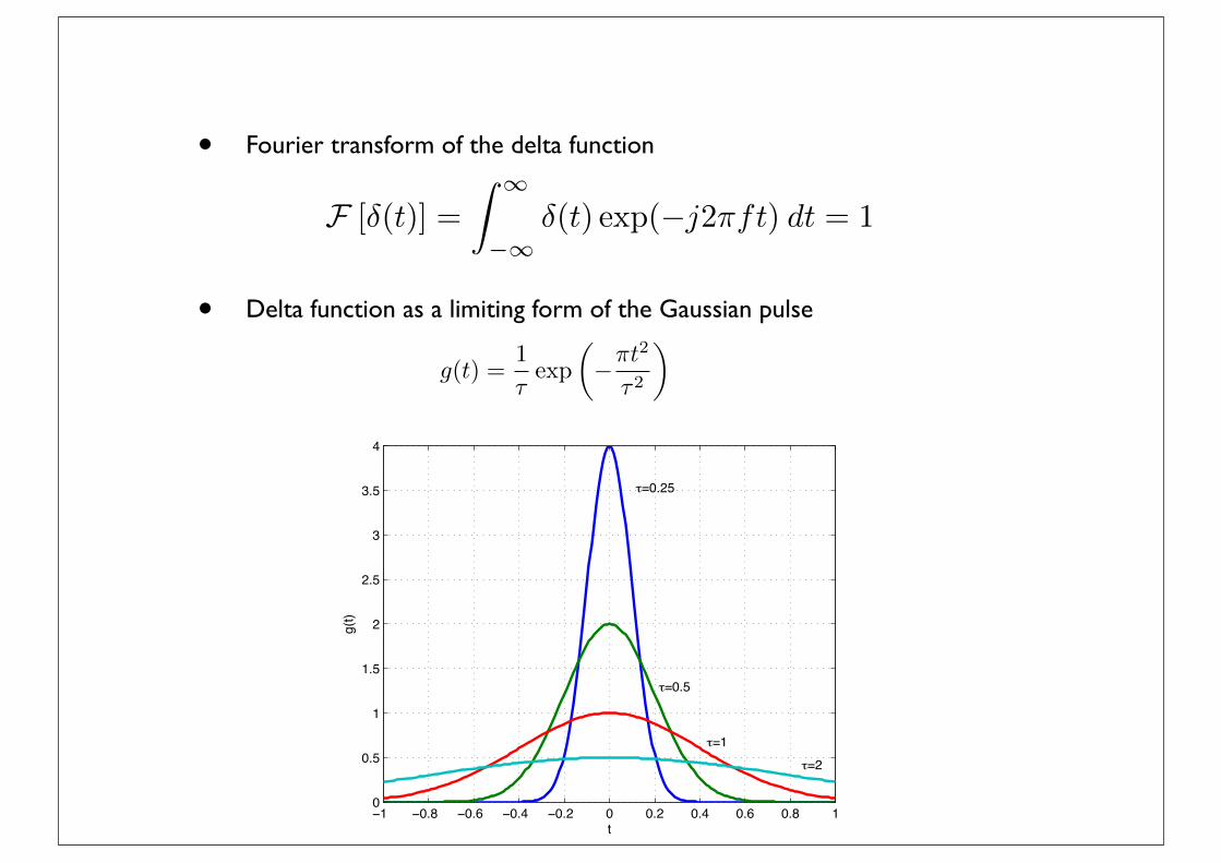
• Fourier transform of the delta function

• Delta function as a limiting form of the Gaussian pulse

F [�(t)] =

Z 1

�1�(t) exp(�j2⇥ft) dt = 1

g(t) =1

⇥exp

✓��t2

⇥2

◆

−1 −0.8 −0.6 −0.4 −0.2 0 0.2 0.4 0.6 0.8 10

0.5

1

1.5

2

2.5

3

3.5

4

t

g(t)

o=0.25

o=0.5

o=1

o=2

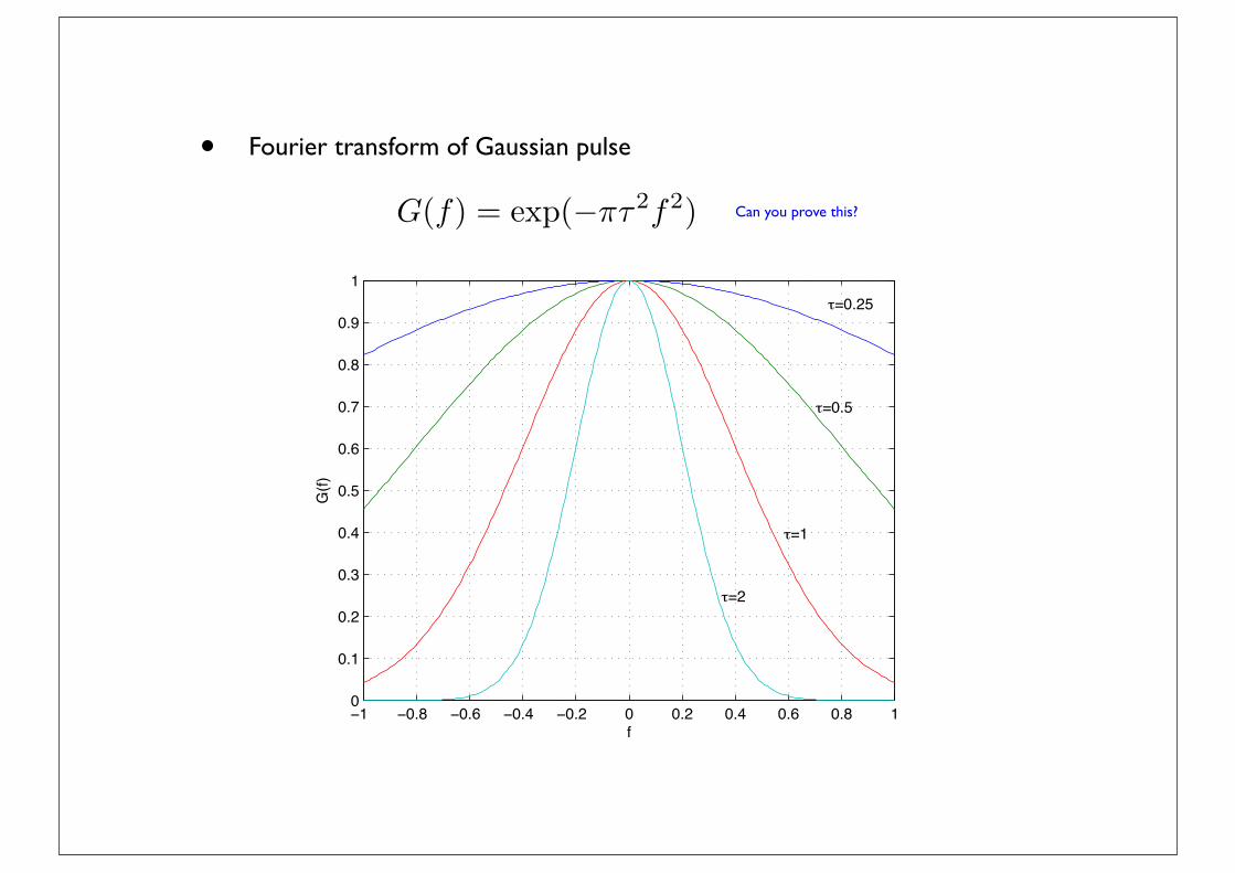
• Fourier transform of Gaussian pulse

G(f) = exp(��⇥2f2)

−1 −0.8 −0.6 −0.4 −0.2 0 0.2 0.4 0.6 0.8 10

0.1

0.2

0.3

0.4

0.5

0.6

0.7

0.8

0.9

1

o=2

o=1

o=0.5

o=0.25

f

G(f)

Can you prove this?

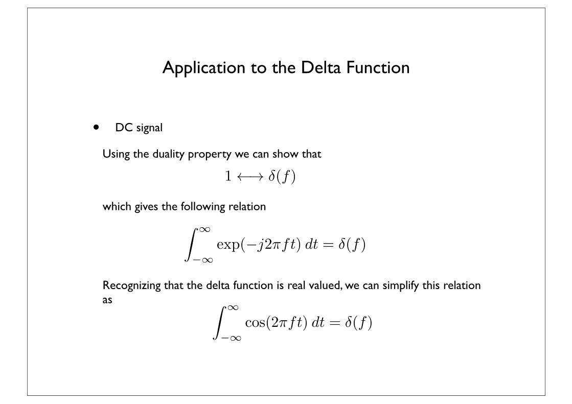
• DC signal

Using the duality property we can show that

which gives the following relation

Recognizing that the delta function is real valued, we can simplify this relation as

Application to the Delta Function

1 ! �(f)

Z 1

�1exp(�j2⇥ft) dt = �(f)

Z 1

�1cos(2⇥ft) dt = �(f)

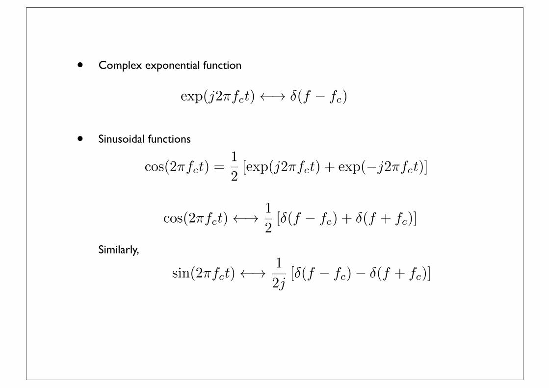
• Complex exponential function

• Sinusoidal functions

Similarly,

exp(j2⇥fct) ! �(f � fc)

cos(2�fct) =1

2

[exp(j2�fct) + exp(�j2�fct)]

cos(2⇥fct) !1

2

[�(f � fc) + �(f + fc)]

sin(2⇥fct) !1

2j[�(f � fc)� �(f + fc)]

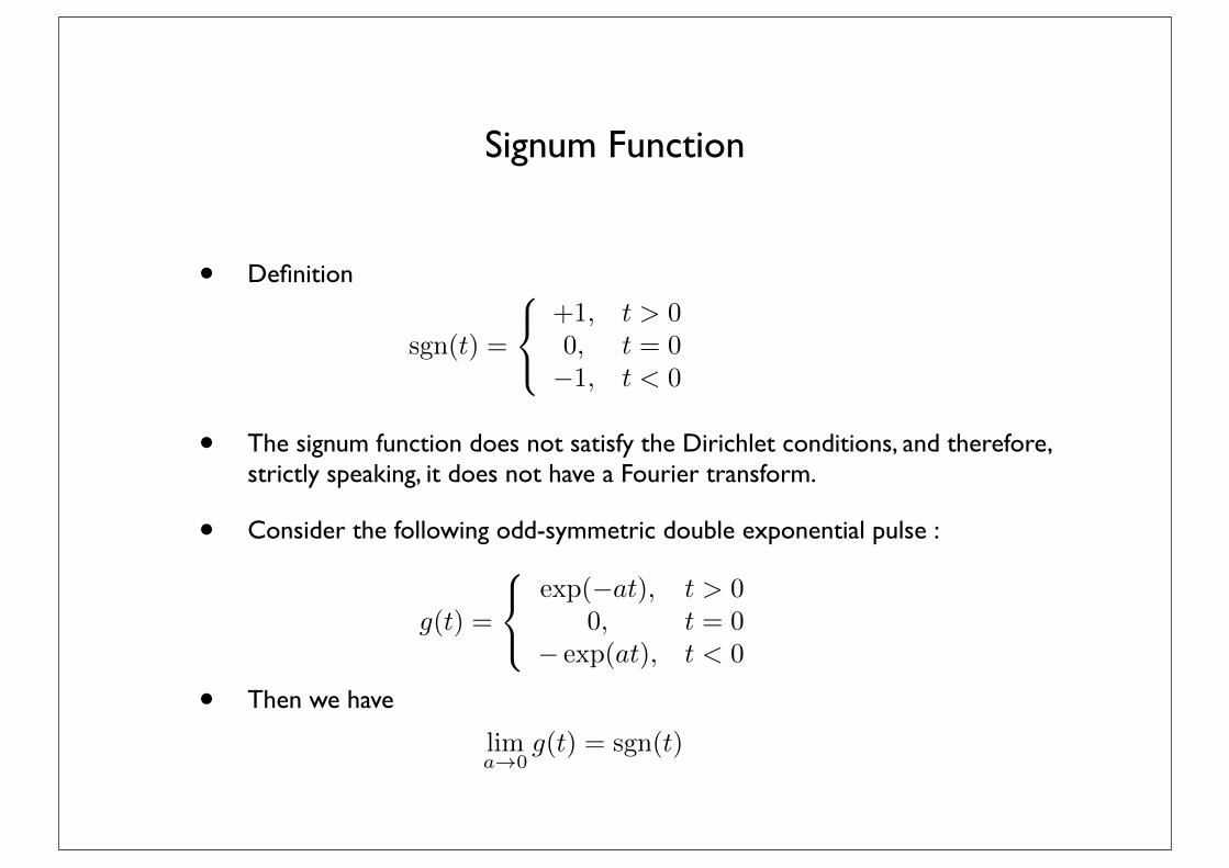
Signum Function

• Definition

• The signum function does not satisfy the Dirichlet conditions, and therefore, strictly speaking, it does not have a Fourier transform.

• Consider the following odd-symmetric double exponential pulse :

• Then we have

sgn(t) =

8<

:

+1, t > 00, t = 0�1, t < 0

g(t) =

8<

:

exp(�at), t > 0

0, t = 0

� exp(at), t < 0

lima!0

g(t) = sgn(t)

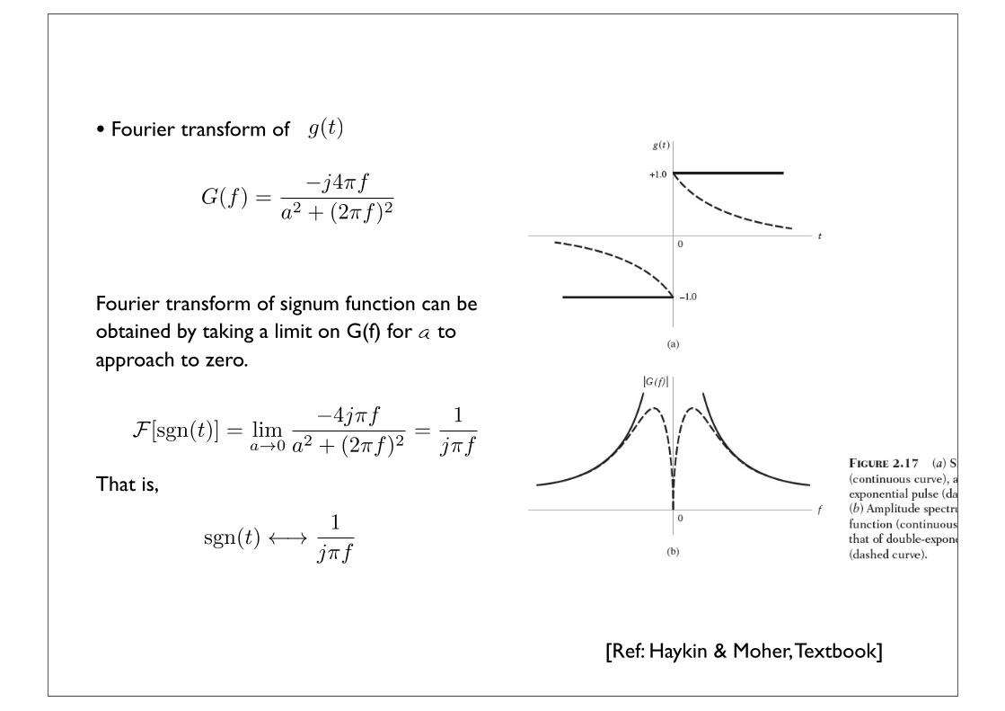
• Fourier transform of

Fourier transform of signum function can be obtained by taking a limit on G(f) for a to approach to zero.

That is,

G(f) =�j4�f

a2 + (2�f)2

g(t)

F [sgn(t)] = lima!0

�4j�f

a2 + (2�f)2=

1

j�f

sgn(t) ! 1

j�f

[Ref: Haykin & Moher, Textbook]

Unit Step Function

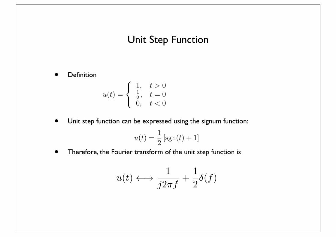
• Definition

• Unit step function can be expressed using the signum function:

• Therefore, the Fourier transform of the unit step function is

u(t) =

8<

:

1, t > 012 , t = 00, t < 0

u(t) =1

2[sgn(t) + 1]

u(t) ! 1

j2⇥f+

1

2�(f)

Fourier Transform of Periodic Signals

• The periodic signals do not satisfy the Dirichlet conditions so, strictly speaking, they do not have Fourier transform. However, using the delta function, we can obtain the Fourier transform of the periodic signals.

• Periodic signal with fundamental period :

• Then we can express it in Fourier series form given as

T0 gT0(t)

gT0(t) =1X

n=�1cn exp(j2�nf0t)

cn =

1

T0

Z T0/2

�T0/2gT0(t) exp(�j2�nf0t) dtwhere

f0 =1

T0

• Define as a function equals over one period

• Also, we have

• Accordingly we may rewrite the Fourier coefficients as

which gives

g(t) gT0(t)

g(t) =

⇢gT0(t), �T0

2 t T02

0, elsewhere

gT0(t) =1X

m=�1g(t�mT0)

cn = f0

Z 1

�1g(t) exp(�j2�nf0t) dt = f0G(nf0)

gT0(t) = f0

1X

n=�1G(nf0) exp(j2�nf0t)

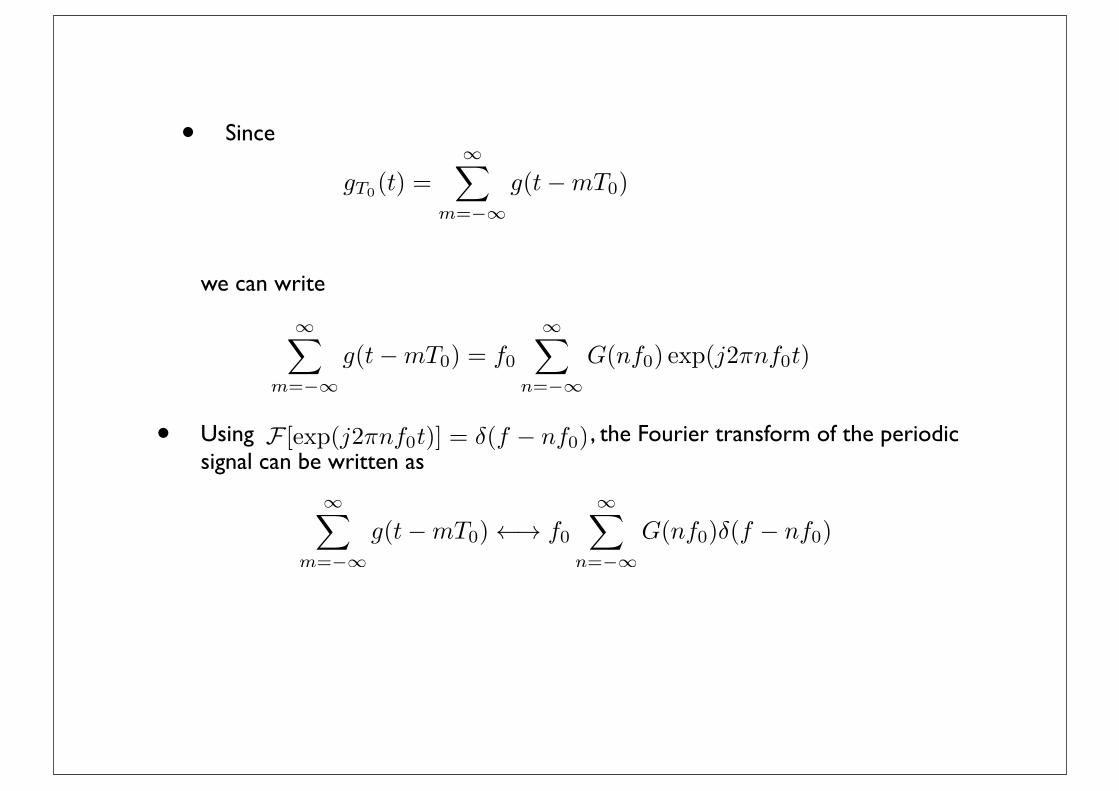
• Since

we can write

• Using , the Fourier transform of the periodic signal can be written as

gT0(t) =1X

m=�1g(t�mT0)

1X

m=�1g(t�mT0) = f0

1X

n=�1G(nf0) exp(j2�nf0t)

F [exp(j2⇥nf0t)] = �(f � nf0)

1X

m=�1g(t�mT0) ! f0

1X

n=�1G(nf0)�(f � nf0)

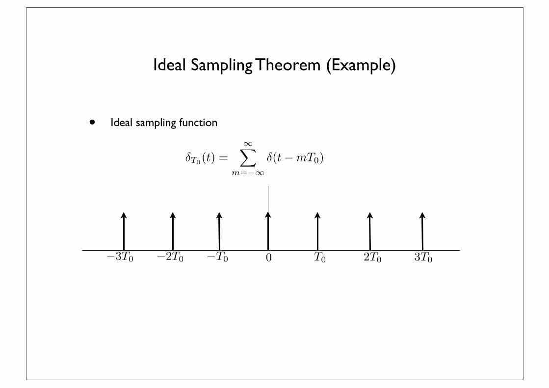
• Ideal sampling function

Ideal Sampling Theorem (Example)

�T0(t) =1X

m=�1�(t�mT0)

�T0�2T0�3T0 3T02T0T00

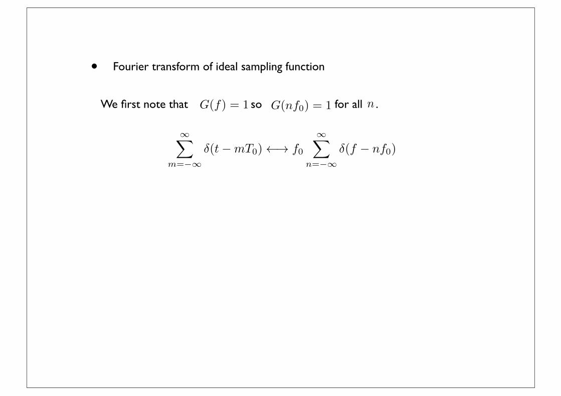
• Fourier transform of ideal sampling function

We first note that so for all .G(f) = 1 G(nf0) = 1 n

1X

m=�1�(t�mT0) ! f0

1X

n=�1�(f � nf0)

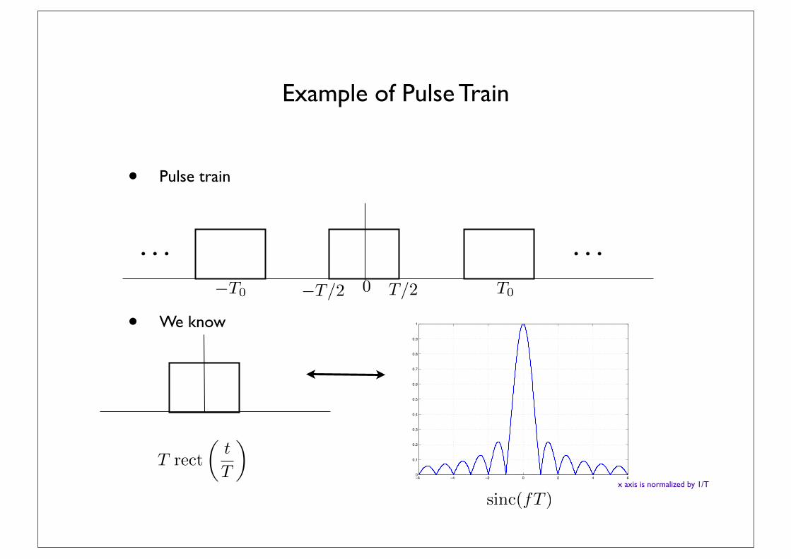
• Pulse train

• We know

Example of Pulse Train

T0�T0 0�T/2 T/2

. . .. . .

−6 −4 −2 0 2 4 60

0.1

0.2

0.3

0.4

0.5

0.6

0.7

0.8

0.9

1

sinc(fT )

T rect

✓t

T

◆

x axis is normalized by 1/T

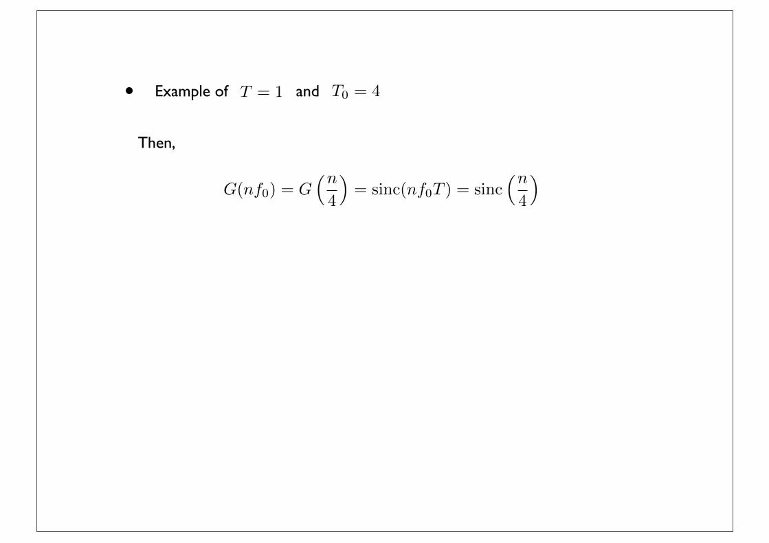
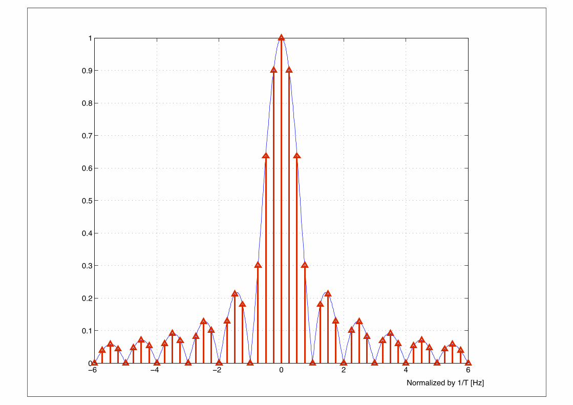
• Example of and

Then,

T = 1 T0 = 4

G(nf0) = G⇣n4

⌘= sinc(nf0T ) = sinc

⇣n4

⌘

−6 −4 −2 0 2 4 60

0.1

0.2

0.3

0.4

0.5

0.6

0.7

0.8

0.9

1

Normalized by 1/T [Hz]

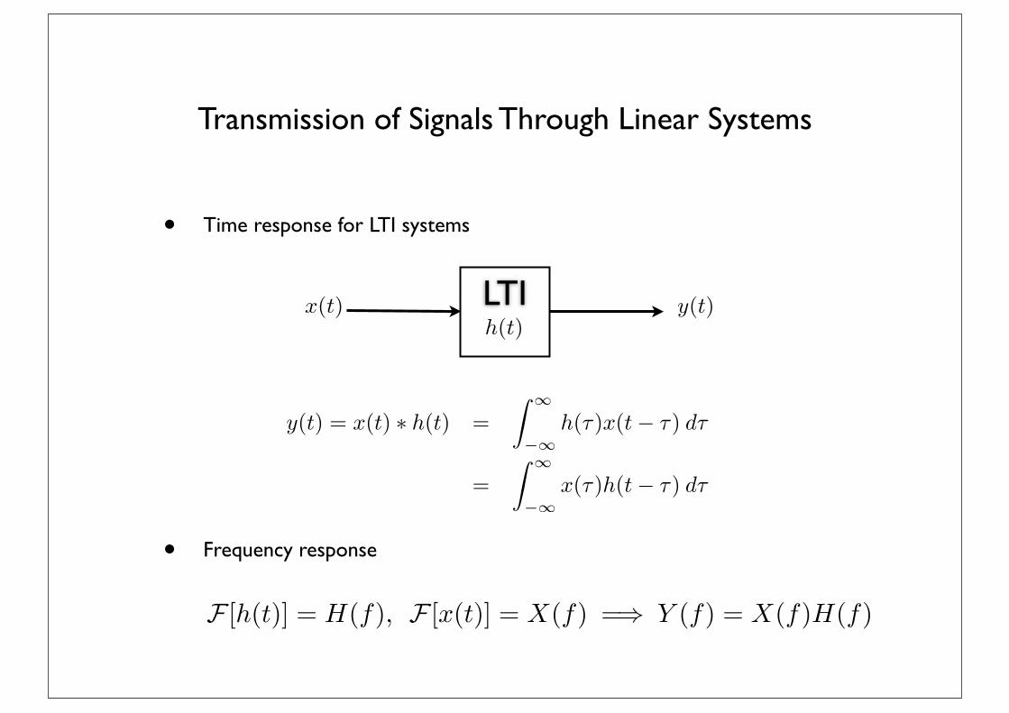
Transmission of Signals Through Linear Systems

• Time response for LTI systems

• Frequency response

LTIx(t) y(t)

h(t)

y(t) = x(t) ⇤ h(t) =

Z 1

�1h(�)x(t� �) d�

=

Z 1

�1x(�)h(t� �) d�

F [h(t)] = H(f), F [x(t)] = X(f) =� Y (f) = X(f)H(f)

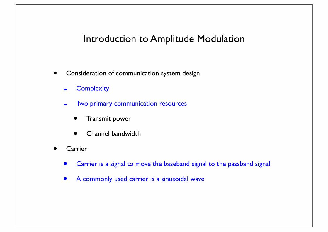
Introduction to Amplitude Modulation

• Consideration of communication system design

- Complexity

- Two primary communication resources

• Transmit power

• Channel bandwidth

• Carrier

• Carrier is a signal to move the baseband signal to the passband signal

• A commonly used carrier is a sinusoidal wave

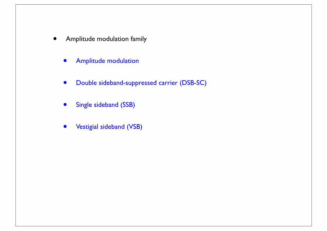
• Amplitude modulation family

• Amplitude modulation

• Double sideband-suppressed carrier (DSB-SC)

• Single sideband (SSB)

• Vestigial sideband (VSB)

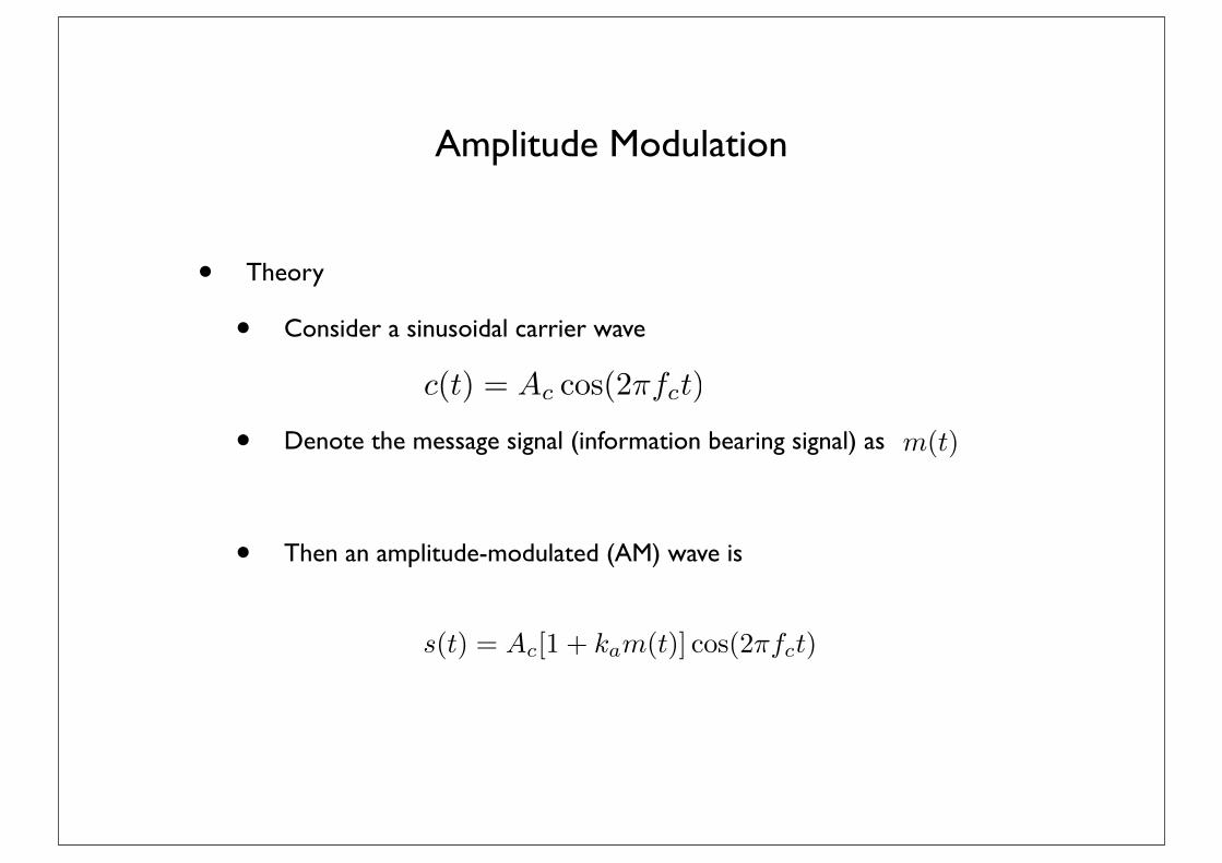
• Theory

• Consider a sinusoidal carrier wave

• Denote the message signal (information bearing signal) as

• Then an amplitude-modulated (AM) wave is

Amplitude Modulation

c(t) = Ac cos(2�fct)

m(t)

s(t) = Ac[1 + kam(t)] cos(2�fct)

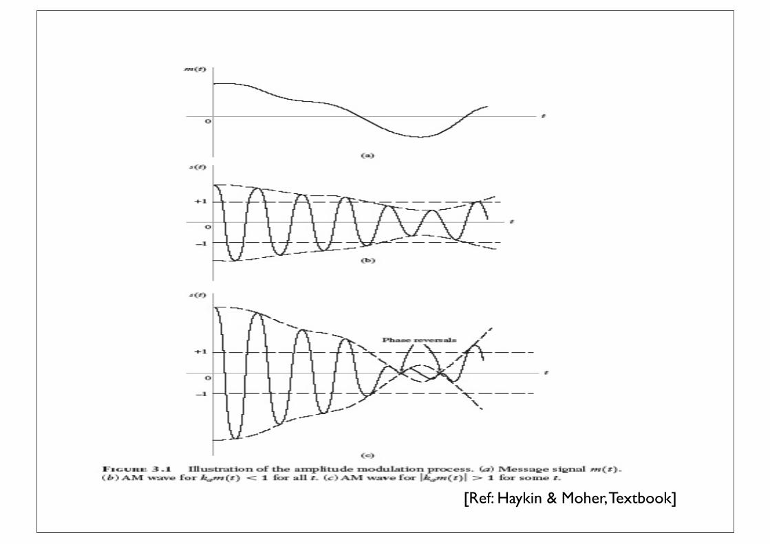
[Ref: Haykin & Moher, Textbook]