Embed Size (px)
Citation preview
0018-9286 (c) 2015 IEEE. Personal use is permitted, but republication/redistribution requires IEEE permission. See http://www.ieee.org/publications_standards/publications/rights/index.html for more information.
This article has been accepted for publication in a future issue of this journal, but has not been fully edited. Content may change prior to final publication. Citation information: DOI 10.1109/TAC.2015.2502781, IEEETransactions on Automatic Control
IEEE TRANSACTIONS ON AUTOMATIC CONTROL, VOL. ?, NO. ?, OCTOBER 2014 1
Formal Verification of Stochastic Max-Plus-Linear SystemsSadegh Esmaeil Zadeh Soudjani, Dieky Adzkiya, and Alessandro Abate
Abstract—This work investigates the computation of finiteabstractions of Stochastic Max-Plus-Linear (SMPL) systems andtheir formal verification against general bounded-time lineartemporal specifications. SMPL systems are probabilistic exten-sions of discrete-event MPL systems, which are widely employedfor modeling engineering systems dealing with practical timingand synchronization issues. Departing from the standard existingapproaches for the analysis of SMPL systems, we newly proposeto construct formal, finite abstractions of a given SMPL system:the SMPL system is first re-formulated as a discrete-time Markovprocess, then abstracted as a finite-state Markov Chain (MC).The derivation of precise guarantees on the level of the intro-duced formal approximation allows us to probabilistically modelcheck the obtained MC against bounded-time linear temporalspecifications (which are of rather general applicability), andto reliably export the obtained results over the original SMPLsystem. The approach is practically implemented on a dedicatedsoftware and is elucidated and run over numerical examples.
Index Terms—Max-plus-linear systems, max-plus algebra,discrete-time stochastic processes, continuous-state processes,probabilistic model checking, linear-time logic, finite abstractions.
I. BACKGROUND AND GOALS
MAX-PLUS-LINEAR (MPL) systems are a class ofdiscrete-event systems [1], [2] with a continuous state
space characterizing the timing of the underlying sequentialdiscrete events. MPL systems are used to describe the tim-ing synchronization between interleaved processes, under theassumption that timing events are dependent linearly (withinthe max-plus algebra) on previous event occurrences. MPLsystems are widely employed in the analysis and schedulingof infrastructure networks, such as communication and railwaysystems [3], or production and manufacturing lines [4], [5].
Stochastic Max-Plus-Linear (SMPL) systems [6], [7], [8]are MPL systems where the time interval between successiveevent occurrences (in the examples above, the transportation,processing, or production times) are now characterized byrandom quantities. In practical applications SMPL systems areevidently more realistic than simpler MPL ones: for instance ina model for a railway network, train running times depend onimperceptible changes in driver behavior, on hardly predictableweather conditions, and on volatile passenger numbers at
S. Esmaeil Zadeh Soudjani and A. Abate are with the Department ofComputer Science, University of Oxford, Oxford OX1 2JD, U.K. e-mail:{Sadegh.Soudjani,Alessandro.Abate}@cs.ox.ac.uk.
D. Adzkiya is with the Department of Mathematics, InstitutTeknologi Sepuluh Nopember, Surabaya 60111, Indonesia e-mail:[email protected].
The first two authors have equally contributed to this work.This work has been supported by the European Commission Marie Curie
grant MANTRAS 249295, IAPP project AMBI 324432, and by the John FellOUP Research Fund.
stations: as such they can arguably be more suitably modeledby random variables than fixed deterministic delays.
We are interested in analyzing general dynamical propertiesof SMPL systems. Only a few approaches have been developedin the literature, and focus on the study of the steady-statebehavior of SMPL systems, for example employing Lyapunovexponents and asymptotic growth rates [9], [10], [11], [12],[13], [14]. The Lyapunov exponent of an SMPL system isanalogous to the max-plus eigenvalue for an autonomous MPLsystem [11, Sec. 7.3]. The series expansion formula of aLyapunov exponent has been discussed in [12], [13]. Theasymptotic behavior of sequences of states of SMPL systemsis analyzed in [14]. The computation of Lyapunov exponentof SMPL systems under some assumptions has been studiedin [9], and later extended to approximate computations underother technical assumptions in [10, p. 251]. The application ofmodel predictive control and system identification to SMPLsystems is studied in [15], [16]. An alternative approachto model uncertainties in MPL systems using intervals isdiscussed in [17], [18], [19].
As we mentioned in the previous paragraph, the existingworks on SMPL systems focus on the study of steady-statebehaviors: as such, existing approaches cannot distinguishtime-dependent dynamical properties of trajectories outsidetheir steady state. This motivates us to develop a new approachfor studying general dynamical properties of SMPL systemsvia formal verification. The formal verification approach isbased on developing finite-state abstractions and, whilst quitedifferent in the nature of the used techniques and of the modelsof interest, can be related to the approach discussed in [20]for (deterministic) MPL systems. As discussed shortly, heregeneral dynamical properties are expressed as formulae in atemporal logic, and verification is attained via (probabilistic)model checking. Furthermore this work can also be seenas broad extension of [3, Ch. 9], where the authors discussthe sensitivity of deterministic MPL systems w.r.t. a periodictimetable against disturbances: this contribution focuses onverifying general behaviors of SMPL systems w.r.t. a periodictimetable.
Verification techniques and tools for deterministic, discrete-time, finite-state systems have been widely investigated anddeveloped in the past decades [21], often by means of modelchecking [22]. The application of formal methods to stochasticmodels is typically limited to discrete-state structures, eitherin continuous or in discrete time [22], [23]. Continuous-spacemodels on the other hand require the use of finite abstractions,as it is classically done for example with finite bisimulationsof timed automata [24]. With focus on stochastic models withcontinuous state space, as is the case for SMPL systems,numerical schemes based on Markov Chain (MC) approxi-
0000–0000/00$00.00 c© 2015 IEEE
0018-9286 (c) 2015 IEEE. Personal use is permitted, but republication/redistribution requires IEEE permission. See http://www.ieee.org/publications_standards/publications/rights/index.html for more information.
This article has been accepted for publication in a future issue of this journal, but has not been fully edited. Content may change prior to final publication. Citation information: DOI 10.1109/TAC.2015.2502781, IEEETransactions on Automatic Control
IEEE TRANSACTIONS ON AUTOMATIC CONTROL, VOL. ?, NO. ?, OCTOBER 2014 2
mations of stochastic systems have been introduced in [25],[26], and applied to the approximate study of probabilisticreachability or invariance in [27], [28], however these finiteabstractions do not come with explicit error bounds and assuch their use cannot lead to certified guarantees. On thecontrary in [29], [30], a technique with formal guarantees hasbeen introduced to provide formal abstractions of discrete-time, continuous-space Markov models, with the objective ofinvestigating their probabilistic invariance [29] by employingprobabilistic model checking algorithms over a finite-state MC[30]. In view of scalability and of generality, the approachhas been improved in [31], [32] and applied to ProbabilisticComputation Tree Logic (PCTL) properties [33], [34]. Fur-thermore the abstraction approach proposed in [35] allowsconstructing a single abstraction to be then used for verifyingany bounded linear temporal specification. Interestingly, theseprocedures have been shown [36] to introduce an approximateprobabilistic bisimulation of the concrete model [37], whichreinforces the quantitative relationship between concrete andabstract models.
Contributions: The aim of this work is to formally verifySMPL systems w.r.t. a periodic timetable via probabilisticmodel checking, and in particular to characterize and tocompute the satisfiability of Bounded Linear Temporal Logic(BLTL) formulae [38]. More precisely, for any allowable initialevent time, we determine the probability that the time differ-ence between the occurrence of events and a deterministicperiodic timetable satisfies a given BLTL formula (cf. SectionII-C). BLTL formulae are a class of Linear Temporal Logic(LTL) formulae where time horizon of the specifications isfinite. LTL formulae have been widely used to characterizedynamical properties of numerous models, such as discrete-time linear systems [39], stochastic systems [40], [41], andMarkov decision processes [42]. A number of interestingdynamical properties can be expressed as BLTL formulae,e.g. finite-time invariance, finite-time reachability, finite-timereach-avoid, or properties expressed as finite strings overautomata.
The approach works as follows. We first interpret a givenSMPL system as a discrete-time Markov process, as first sug-gested by [7], [8]. Then we adapt the techniques in [30], [32],[35] to the structure of the SMPL system, in order to generate afinite abstraction in the form of a finite-state MC, together withguarantees on the level of approximation introduced in the pro-cess. The formal approximation is guaranteed to hold over anyBLTL formula [35]. The BLTL property over the obtained MCcan then be analyzed via probabilistic model checking [22] andcomputed via existing software [43], [44]. The result obtainedfrom the model checking software is then combined with theapproximation guarantees, in order to obtain the probabilitythat the concrete (original) SMPL system satisfies the givenproperty. Throughout the manuscript we discuss the structuralassumptions and computational requirements underpinning ourresults, and examine relaxations and algorithmic improvementsaimed towards generalization and scalability.
In order to further elucidate the approach, we discuss thecomputation of finite-horizon probabilistic invariance, hereencoded as a simple BLTL formula, of an SMPL system: more
precisely, for any given occurrence time for the initial event,we determine the probability that the time associated with theoccurrence of N consecutive events remains close to a givendeterministic N -step timetable.
Finally, we conclude by discussing an alternative techniquebased on the following approach: first, we approximate theoriginal density functions by piecewise polynomial densityfunctions; in the second step, the value function associatedwith the approximated density functions is computed explicitlyusing a computer algebra program. We compare the perfor-mance of this technique and the abstraction approach: ourexperiments suggest that the abstraction approach at the coreof this work is more scalable, thus reinforcing its potential forapplications.
Structure of this article: The article is structured as fol-lows. Initially, Section II-A introduces the SMPL formalism,whereas Section II-C presents the problem of probabilisticmodel checking of SMPL systems against BLTL specifi-cations. Section III discusses the formal abstraction of anSMPL system as a Markov chain. Section IV describes thequantification of the abstraction error and presents numericalexamples, focused on the probabilistic invariance problem.An alternative formal approach for the computation of thesolution of the probabilistic invariance problem is discussedin Section V, which is based on the approximation of thedensity functions with piecewise polynomials. Finally, SectionVI concludes this work with future research directions.
Related work by the authors: This manuscript representsan extension and a completion of the results in [45]: there finiteabstraction techniques are constructed exclusively towards thesolution of the probabilistic invariance problem. This workgeneralizes [45] and develops abstractions of SMPL systemsfor model checking against general BLTL specifications. Wefurther elaborate on extensions geared towards computability,and in particular provide a formulation of the abstractionerror that is dimension-dependent, and, as such, parallelizable.Moreover, we discuss an alternative formal approach forcomputation of the solution of the probabilistic invarianceproblem based on approximation of the density functions withpiecewise-polynomial ones.
II. MODELS AND PROBLEM STATEMENT
We introduce the basics of max-plus algebra and of au-tonomous SMPL systems, and discuss probabilistic modelchecking of SMPL systems against BLTL specifications, a goalthat will be further elaborated throughout the article.
A. Modeling: Stochastic Max-Plus-Linear Systems
The notations N and Nn represent the whole positive inte-gers {1, 2, . . .} and the first n positive integers {1, 2, . . . , n},respectively. We use bold letters to denote vectors and indexedletters for the elements of the vector, for instance x =[x1, . . . , xn]
T . Furthermore we define Rε and ε respectively asR∪{ε} and −∞. For α, β ∈ Rε, introduce the two operations
α⊕ β = max{α, β} and α⊗ β = α+ β,
0018-9286 (c) 2015 IEEE. Personal use is permitted, but republication/redistribution requires IEEE permission. See http://www.ieee.org/publications_standards/publications/rights/index.html for more information.
This article has been accepted for publication in a future issue of this journal, but has not been fully edited. Content may change prior to final publication. Citation information: DOI 10.1109/TAC.2015.2502781, IEEETransactions on Automatic Control
IEEE TRANSACTIONS ON AUTOMATIC CONTROL, VOL. ?, NO. ?, OCTOBER 2014 3
where the element ε is considered to be absorbing w.r.t. ⊗[11, Definition 3.4], namely α ⊗ ε = ε for all α ∈ Rε. Therules for the order of evaluation of the max-algebraic operatorscorrespond to those in the conventional algebra: max-algebraicmultiplication ⊗ has a higher precedence than max-algebraicaddition ⊕ [11, Sec. 3.1].
The basic max-algebraic operations are extended to matricesas follows. If A,B ∈ R
m×nε ; C ∈ R
m×pε ; D ∈ R
p×nε ; and
α ∈ Rε, then
[α⊗A]ij = α⊗Aij = α+Aij ,
[A⊕B]ij = Aij ⊕Bij = max{Aij , Bij},
[C ⊗D]ij =
p⊕
k=1
Cik ⊗Dkj = maxk∈{1,...,p}
{Cik +Dkj},
for each i ∈ Nm and j ∈ Nn. Notice the analogy between ⊕,⊗ and respectively +, × for matrix and vector operations inthe conventional algebra. In this paper the usual multiplication× is usually omitted, whereas the max-algebraic multiplication⊗ is always written explicitly. Given m ∈ N, the m-thmax-algebraic power of A ∈ R
n×nε is denoted by A⊗m
and corresponds to A ⊗ · · · ⊗ A (m times). Notice thatmax-algebraic power has higher precedence than ⊗ and ⊕;A⊗0 is an n-dimensional max-plus identity matrix, i.e. thediagonal and non-diagonal elements are 0 and ε, respectively.In this paper, the following notation is adopted for reasons ofconvenience. A vector with each component being equal to 0(resp., −∞) is also denoted by 0 (resp., ε).
An autonomous SMPL system is defined as:
x(k + 1) = A(k)⊗ x(k), (1)
where x(k) = [x1(k), . . . , xn(k)]T ∈ R
n; each entry ofthe state matrix A(k) either equals the constant ε, or is anindependent and identically distributed random variable w.r.t.k ∈ N, taking values on the real line; and further Aij(·) areindependent for all i, j ∈ Nn. The random sequence {Aij(·)}is then characterized by a given density function tij(·) andcorresponding distribution function Tij(·) (cf. Theorem 1below). In (1) the independent variable k denotes an increasingdeterministic occurrence index, whereas the state variable x(k)defines the (continuous) time of the k-th occurrence of thediscrete events. The state component xi(k) denotes the timeof the k-th occurrence of the i-th event. In this work, theoccurrence time of all events is a real number because the statespace is Rn (rather than R
nε ): in order to guarantee x(k) ∈ R
n
for all k, the random matrix A has to be regular (or row-finite)[3, Sec. 1.2], namely A contains at least one element differentfrom ε in each row. Since this article is based exclusively onautonomous (that is, not non-deterministic) SMPL systems,the adjective will be dropped for simplicity.
In contrast with SMPL systems, deterministic MPL systemsare defined according to (1) where the state matrix A(k)is given and event-invariant (independent of k). Under anatural irreducibility condition [11, Definition 2.13] on matrixA, the deterministic MPL system admits periodic regimes,namely there exists a finite sequence of (max-plus) linearly-independent vectors {x1,x2, . . . ,xµ} such that xk+1 = A ⊗xk, k ∈ Nµ−1, and there is a constant d that satisfies
A⊗xµ = d⊗x
1. The parameter d and corresponding vectorsfor the periodic regime x
1,x2, . . . ,xµ represent the max-pluseigenvalue and its associated eigenvectors of matrix A⊗µ,respectively [6, Sec. 2.5.3]. Such periodic regimes are essentialingredients in the analysis and design of timetables for realapplications [46] modeled as MPL systems.
Example 1: Consider the following SMPL system represent-ing a simple railway network between two connected stations.The state variables xi(k) for i ∈ N2 denote the time of thek-th departure at station i:
x(k + 1) = A(k)⊗ x(k),
=
[2 + e11(k) 5 + e12(k)3 + e21(k) 3 + e22(k)
]
⊗ x(k),
or equivalently,
x1(k + 1) = max{2 + e11(k) + x1(k), 5 + e12(k) + x2(k)},
x2(k + 1) = max{3 + e21(k) + x1(k), 3 + e22(k) + x2(k)},
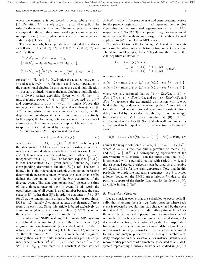
where we have assumed that e11(·) ∼ Exp(2), e12(·) ∼Exp(4/5), e21(·) ∼ Exp(4/3), and e22(·) ∼ Exp(4/3), andExp(λ) represents the exponential distribution with rate λ.Notice that Aij(·) denotes the traveling time from station jto station i and amounts to a deterministic constant plus adelay modeled by the random variable eij(·). A few sampletrajectories of the SMPL system, initialized at x(0) = [1, 0]T ,are displayed in Fig. 1 (left). Note that when all random delaysare assumed to be equal to zero, the resulting deterministicsystem
s(k + 1) = Ad ⊗ s(k), Ad =
[2 53 3
]
, s(0) = x(0), (2)
admits the unique solution s(k) = s(0) + dk = [1+ 4k, 4k]T ,where d = 4 is the max-plus eigenvalue of matrix Ad,and s(0) = [1, 0]T is a corresponding eigenvector of thedeterministic MPL system. Then the initial condition {s(0)}is associated with a periodic regime with period µ = 1, andthe associated periodic trajectory can be used as a timetable(cf. Section II-B) for the train departures. Note that in thisparticular example the increasing sequence {s(k)} providesa lower bound on the SMPL trajectories x(k), due to thepositive supports of the density functions for the delays eij(·),as visible in Fig. 1 (left).
B. Properties of Interest
Let us consider events that are scheduled to occur periodi-cally, that is assume there is a periodic timetable where eachevent is repeated at regular intervals characterized by the cycletime d ∈ R. For instance a periodic railway timetable definesthe scheduled arrival and departure times within a basic periodof length d for each periodic train line at all served stations. Asdiscussed in Section I, stochastic delays due to transportationtimes and train interactions are an unavoidable characteristicof real-world railway networks: it is therefore meaningfulto study and analyze properties of a railway timetable w.r.t.daily transportation time variations. For instance, stability andrecoverability properties of a timetable associated to an SMPLsystem representing a railway network are studied in [46]. In
0018-9286 (c) 2015 IEEE. Personal use is permitted, but republication/redistribution requires IEEE permission. See http://www.ieee.org/publications_standards/publications/rights/index.html for more information.
This article has been accepted for publication in a future issue of this journal, but has not been fully edited. Content may change prior to final publication. Citation information: DOI 10.1109/TAC.2015.2502781, IEEETransactions on Automatic Control
IEEE TRANSACTIONS ON AUTOMATIC CONTROL, VOL. ?, NO. ?, OCTOBER 2014 4
0 2 4 6 8 100
20
40
60
k
x1
0 2 4 6 8 10
0
10
k
z1
0 2 4 6 8 100
20
40
60
k
x2
0 2 4 6 8 10
0
10
k
z2
Fig. 1. The left and right plots represent 100 sample trajectories of theSMPL system in Examples 1 and 2 for 10 discrete steps (horizontal axis),respectively. Notice the different scales for the vertical axes.
this work, we consider probabilistic model checking of theSMPL system in (1) against a specification w.r.t. a periodictimetable. More specifically, for each possible time of initialoccurrence of all the events (xi(0), i ∈ Nn), we are interestedin determining the probability that the difference of the timeof k-th occurrence of all events (x(k)) and the correspondingtime of the periodic timetable satisfies a given BLTL formula,for k ∈ NN ∪ {0}. For instance, we may want to determinethe probability that the time of the occurrence of all eventsis at least 5 time units ahead of the corresponding eventsin the periodic timetable, as well as at most 5 time unitsbehind it: this example deals with an invariance property,where the (bounded) invariant set is defined as the desiredtime of occurrence of all events w.r.t. the periodic timetable.
Let us formally define a periodic timetable: s(·) is called aperiodic timetable with cycle time d > 0 and (arbitrary) initialtime s(0) = s0 ∈ R
n, if the successive scheduled event timesare given by the deterministic MPL system s(k+1) = d⊗s(k).In our analysis the periodic timetable can be freely selected:for instance, it can be an arbitrary function of the periodicregimes of the SMPL system in the absence of stochasticdelays (cf. (2) in Example 1, where a periodic trajectory isgenerated from a fixed initial condition in the eigenspace ofthe model). The mean behavior of the SMPL system, whichis proved in general to be eventually periodic [46], may alsobe selected as the given timetable.
Since we are interested in delays of event occurrences w.r.t.the given timetable, we introduce new variables z(·) defined asthe difference between the states of the original SMPL systemin (1) and those of the periodic timetable s(·), i.e. z(k) =x(k) − s(k), and z(k) = [z1(k), . . . , zn(k)]
T ∈ Rn for k ∈
N ∪ {0}. The dynamics of z(·) are given by
zi(k + 1) = max{Ai1(k)− d+ x1(k)− si(k), . . .. . . , Ain(k)− d+ xn(k)− si(k)},
for i ∈ Nn. From the dynamics of s(k), we obtain si(k) −sj(k) = si(0)−sj(0) for all i, j ∈ Nn and k ∈ N∪{0}. Then
we substitute si(k) = si(0)−sj(0)+sj(k) to the j-th term ofthe equation for zi(k+1), and further substitute xi(k)−si(k)by zi(k) to obtain
zi(k + 1) = max{Ai1(k) + s1(0)− si(0)− d+ z1(k), . . .. . . , Ain(k) + sn(0)− si(0)− d+ zn(k)}.
In matrix notation, the dynamics of the newly introducedSMPL system are then given by
z(k + 1) = [A(k) +D]⊗ z(k), (3)
where D = [dij ]i,j ∈ Rn×n (i.e. dij is the entry of matrix D
at row i and column j), dij = sj(0)− si(0)− d. Notice thatAij(k)⊗dij are independent for all k ∈ N∪{0} and i, j ∈ Nn.The density (resp., distribution) function of Aij(k) ⊗ dijcorresponds to the density (resp., distribution) function ofAij(k) shifted forward of dij units. In (3) the deterministicindex k again denotes an increasing occurrence index, whereasthe state variable z(k) defines the delay w.r.t. the scheduleof the k-th occurrence of all events: in particular the statecomponent zi(k) denotes the delay w.r.t. the schedule of k-thoccurrence of the i-th event. Notice that if the delay is negativethen the event occurs ahead of the schedule, whereas if thedelay is positive then the event occurs behind the schedule.
As confirmed by Example 1, the trajectories of the SMPLsystem (1) are lower bounded by a monotonically increasingsequence under some weak conditions on the density functionstij(·)
1. This condition results in a potentially very large statespace for the state variable x(·). In contrast, the timing ofevents w.r.t. to the timetable, encompassed by z(·), belongsto a substantially smaller set Z: this is beneficial since it willreduce the computational complexity of our abstraction, asdetailed later.
Example 2: Consider the SMPL system in Example 1.Sample trajectories of the new SMPL system associated withs(0) = [0, 0]T and d = 5 are depicted in Fig. 1 (right).
The next theorem shows that, much like the original modelin (1), the new SMPL system can be described as a discrete-time homogeneous Markov process.2 A Markov process is astochastic process where the probability distribution of the nextstate depends only on the current state.
Theorem 1: The SMPL system in (3) is fully characterizedby the following conditional density function
tz(z|z) =n∏
i=1
ti(zi|z) where
ti(zi|z) =n∑
j=1
tij(zi − dij − zj)n∏
k=1k 6=j
Tik(zi − dik − zk)
for i ∈ Nn.The proof of Theorem 1 appears in Appendix A.
1More precisely, it can be shown that if Aij(k) ≥ aij > 0, such thatA = [aij ]i,j is irreducible, then there exists a subsequence of x(k) that isbounded element-wise from below by a monotonically increasing sequence.
2Note that this result can be generalized to multi-periodic timetables,namely timetables characterized by s(k+1) = d⊗ s(k), where d ∈ R
n×n
is a diagonal matrix, whereas in periodic timetables the cycle time is a scalar.However the associated Markov process becomes inhomogeneous, whichgreatly increases the computational complexity of the discussed procedures.
0018-9286 (c) 2015 IEEE. Personal use is permitted, but republication/redistribution requires IEEE permission. See http://www.ieee.org/publications_standards/publications/rights/index.html for more information.
This article has been accepted for publication in a future issue of this journal, but has not been fully edited. Content may change prior to final publication. Citation information: DOI 10.1109/TAC.2015.2502781, IEEETransactions on Automatic Control
IEEE TRANSACTIONS ON AUTOMATIC CONTROL, VOL. ?, NO. ?, OCTOBER 2014 5
C. Problem Statement: Probabilistic Model Checking ofSMPL Systems Against BLTL Formulae
We present some basic definitions to formalize the prob-abilistic model checking problem on the SMPL system in(3). We introduce a set of finitely many atomic propositionsAP and a labeling function L : Z → 2AP . Notation 2AP
denotes the power set of AP . Atomic propositions intuitivelyexpress simple facts about the states of the system, or can bethought of as properties associated to the states (e.g., “initial,”“safe,” or “target” states). The labeling function L relates a setL(z) ∈ 2AP of atomic propositions to any state z ∈ Z . Theset L(z) represents the atomic propositions that are satisfiedby state z.
BLTL is a fragment of LTL, made up of formulae where thetime horizon of the specifications is bounded [35, Sec. 2.4].This class of formulae has been recently employed in statisticalmodel checking of stochastic systems [41]. Recall that an LTLformula consists of atomic propositions, of Boolean connec-tors, and of two temporal modalities: © (pronounced “next”)and U (pronounced “until”). BLTL formulae are instead ob-tained with only the temporal modality ©. More formally,the syntax of BLTL over the set of atomic propositions APis given by the following grammar:
ϕ ::= a | ¬ϕ | ϕ1 ∧ ϕ2 | ©ϕ,
where a ∈ AP . The semantics of BLTL formulae are inheritedfrom those of LTL formulae [47, Sec. 5.1.2].
We define the probabilistic model-checking problem overa BLTL specification as follows. Given the SMPL system in(3), a set of atomic propositions AP , a labeling function L,an initial state z(0) ∈ Z , and a BLTL formula ϕ, find theprobability that the trajectory starting from state z(0) satisfiesϕ:
Pr{z(0) � ϕ}. (4)
BLTL formulae can express well-known bounded-time ver-ification problems, such as probabilistic reachability, reach-avoid, and invariance (safety) [38, p. 220]. In order to makethe discussion as clear as possible, we provide the details ofthe construction of a BLTL formula associated with the sim-plest problem of invariance. The finite-horizon probabilisticinvariance problem amounts to evaluating the probability thata finite execution associated with the initial condition z(0)remains inside a given invariant set A during the finite eventhorizon N , as follows:
Pz0(A) = Pr{z(k) ∈ A for all k ∈ NN ∪ {0}|z(0) = z0},
(5)where A is assumed to be Borel measurable (that is, con-structed from open sets via operations of countable union,countable intersection, and relative complement). Define theset of atomic propositions AP = {a} and the labeling functionas L(z) = {a} if z ∈ A and L(z) = ∅ if z /∈ A. Consider aBLTL formula given by
�≤Na = a ∧©a ∧©© a ∧ · · · ∧©© · · ·©
︸ ︷︷ ︸
Ntimes
a.
Then the probabilistic invariance can be characterized as thefollowing probability: Pr{z(0) � �
≤Na}. This quantity, or
input: SMPL system (3) and labeling function L : Z → 2AP
output: A finite-state MC (P , Tp)1: Select a finite partition of the state space Z of cardinalitym, as Z = ∪m
i=1Zi, such that all states in a partition setsatisfy the same set of atomic propositions
2: For each Zi, select a single representative point zi ∈ Zi
3: Define P = {φi, i ∈ Nm} as the finite state space of theMC
4: Compute the transition probability matrix Tp as
Tp(φi, φj) =
∫
Ξ(φj)
tz(z|zi)dz, for all i, j ∈ Nm.
5: Define the induced labeling function Lp : P → 2AP forthe MC as Lp(φi) = L(zi) for all i ∈ Nm
Fig. 2. Algorithm 2. Generation of a finite-state MC from an SMPL systemand a labeling function L.
more generally the expression in (4), is numerically computedover finite-space models such as Markov chains, via knownexisting software PRISM [43]. An explicit characterizationof probabilistic invariance is provided in Proposition 2 andcan indeed be computed in PRISM. On the other hand, thecharacterization over models of interest in this work requiresthe approach discussed next, and will leverage the softwareFAUST2 [48], to be discussed below.
III. ABSTRACTIONS BY FINITE-STATE MARKOV CHAINS
We resort to the abstraction procedure presented in [30,Sec. 3.1], properly extended to the models under study. Theprocedure generates a finite-state MC (P , Tp) from a givenSMPL system (3), a set of finitely many atomic propositionsAP , and a labeling function L : Z → 2AP . We employ theobtained MC to approximately model check the SMPL systemagainst a given BLTL specification defined over the atomicpropositions AP .
Let P = {φ1, . . . , φm} be a set of finitely many discretestates, and Tp : P ×P → [0, 1] a related transition probabilitymatrix, such that Tp(φi, φj) characterizes the probability oftransitioning from state φi to state φj and thus induces aconditional discrete probability distribution over the finitespace P . Given a labeling function L, the algorithm in Fig. 2provides a procedure to abstract an SMPL system by a finite-state MC.3 The set P = {φ1, . . . , φm} denotes the discretestate space of cardinality m. In Algorithm 2, Ξ : P → 2Z
represents the concretization function, i.e. a set-valued mapthat associates to any discrete state (point) φi ∈ P thecorresponding continuous partition set Zi ⊂ Z .
Remark 1: The bottleneck of Algorithm 2 lies in the com-putation of transition probability matrix Tp (step 4), due to theintegration of kernel tz . The required number of integrationsis m2, where m represents the cardinality of the set of discretestates. This integration can be circumvented if the distributionfunctions Tij(·) for all i, j ∈ Nn have explicit analytical form(e.g. an exponential distribution).
3For simplicity, when referring to an algorithm we will use the term“Algorithm 2” rather than “the Algorithm in Fig. 2.”
0018-9286 (c) 2015 IEEE. Personal use is permitted, but republication/redistribution requires IEEE permission. See http://www.ieee.org/publications_standards/publications/rights/index.html for more information.
This article has been accepted for publication in a future issue of this journal, but has not been fully edited. Content may change prior to final publication. Citation information: DOI 10.1109/TAC.2015.2502781, IEEETransactions on Automatic Control
IEEE TRANSACTIONS ON AUTOMATIC CONTROL, VOL. ?, NO. ?, OCTOBER 2014 6
The abstraction procedure in Algorithm 2 preserves theunderlying labels, and has been shown to introduce an approx-imate probabilistic bisimulation of the concrete model [37],[36]. This means that Algorithm 2 can be applied to abstract anSMPL system as a finite-state MC, regardless of the particularBLTL specification. As discussed below, the quantification ofthe abstraction error in Section IV requires that the state spaceZ is bounded.
Considering the obtained finite-state, discrete-time MC(P , Tp) and the induced labeling function Lp, the BLTL modelchecking problem amounts to evaluating the probability thatan execution associated with the initial condition φ(0) ∈ Psatisfies a given BLTL specification ϕ expressed over thelabels induced by function Lp. This can be stated as thefollowing probability:
Pr{φ(0) � ϕ}. (6)
In general, the solution can be obtained by leveraging proba-bilistic model checking software [43], [44]. In the special caseof a BLTL specification representing finite-horizon invariance,the solution can also be characterized using dynamic program-ming, as shown in Section IV-B. The next section discussesthe error associated to the general abstraction procedure, andpresents numerical examples focused on the simple finite-horizon invariance problem.
IV. QUANTIFICATION OF THE ABSTRACTION ERROR
This section starts by precisely defining the error related tothe abstraction procedure, which is due to the approximation ofa continuous concrete model by a finite discrete one. A boundon the abstraction error in [32] is applied to the BLTL modelchecking problem under some structural assumptions, namelyin the case of Lipschitz-continuous density functions, or alter-natively of piecewise Lipschitz-continuous density functions.
The abstraction error is defined as the maximum differencebetween the outcomes obtained by (4) and (6) for any pairof initial conditions z(0) ∈ Z and ξ(z(0)) ∈ P , where theabstraction function ξ : Z → P associates to any point z ∈Z on the SMPL state space, the corresponding discrete stateξ(z) ∈ P . Since an exact computation of this error is notpossible in general, we resort to determining an upper boundof the abstraction error, which is denoted as E. More formally,we are interested in quantifying E that satisfies
|Pr{z(0) � ϕ} − Pr{ξ(z(0)) � ϕ}| ≤ E, (7)
for all z(0) ∈ Z and any BLTL formula ϕ. Notice that thequantification of this error allows making sense of the resultsobtained from model checking the MC (Pr{ξ(z(0)) � ϕ}) forthe verification of the SMPL system (Pr{z(0) � ϕ}).
We raise the following assumption on the SMPL system in(1) and in (3). Recall that the density function of Aij(k)⊗dijin (3) corresponds to the density function of Aij(k) in (1)shifted dij units forward.
Assumption 1: The density functions tij(·) for i, j ∈ Nn arebounded:
tij(z) ≤Mij for all z ∈ R.
Assumption 1 implies that the distribution functions Tij(·)for i, j ∈ Nn are Lipschitz-continuous. Recall that the (global)Lipschitz constant of a one-dimensional function can becomputed as the maximum of the absolute value of the firstderivative of the function. Thus
|Tij(z)− Tij(z′)| ≤Mij |z − z′| for all z, z′ ∈ R.
For the computation of the bound on the abstraction error,we use the following result based on [32], which has inspiredmost of this work.
Proposition 1 ([32, pp. 933-934]): Suppose Assumption 1holds and the density function tz(z|z) satisfies the condition∫
Z
|tz(z|z)− tz(z|z′)|dz ≤ H‖z− z
′‖ for all z, z′ ∈ Z,
then an upper bound on the abstraction error in (7) is E =NHδ, where N is the horizon of the specification ϕ and δ =max{‖z− z
′‖ s.t. z, z′ ∈ Zi and i ∈ Nm} is the diameter.The horizon of the BLTL specification is easily computed
on the syntax of the formula [35, Sec. 2.4]. Proposition 1shows that the upper bound on the abstraction error dependson the partition diameter (cf. step 1 of Algorithm 2). Recallthat the cardinality of the partition in step 1 of Algorithm 2 isfinite. Thus in order to guarantee that δ is finite, the state spacehas to be bounded. This restriction requires us to truncate thestate space into a bounded set while maintaining the wholedynamics of the system. In order to do so, assume the densityfunction of the initial state and that of entries of state matrixA have bounded support4. This assumption enables us tocompute bounds on the support of finite trajectories of theSMPL system in (3), which in turn can be used to constructa bounded state space [18]. On the other hand, for someBLTL specifications it is not required to partition the wholestate space: for instance, in the case of invariance only theboundedness of the invariant set is required for the abstractionprocedure.
In the remainder of this section, we first determine theconstant H for Lipschitz-continuous density functions, thengeneralize the result to piecewise Lipschitz-continuous densityfunctions. We reformulate the upper bound on the abstractionerror as a summation of dimension-dependent terms. Finallywe provide a simple application to the study of the probabilis-tic invariance problem.
A. Lipschitz-Continuous Density Functions
Assumption 2: The density functions tij(·) for i, j ∈ Nn
are Lipschitz-continuous, namely there exist finite and positiveconstants hij , such that
|tij(z)− tij(z′)| ≤ hij |z − z′| for all z, z′ ∈ R.
Assumption 2 requires the density functions tij(·) to becontinuous and to have bounded one-sided derivatives.
Under Assumptions 1 and 2, the conditional density functiontz(z|z) is Lipschitz-continuous. This opens up the application
4If instead tij(·) has an unbounded support, we must truncate it to abounded one. This introduces another error on top of the abstraction errorpresented in this section, see [49], [50] for more details.
0018-9286 (c) 2015 IEEE. Personal use is permitted, but republication/redistribution requires IEEE permission. See http://www.ieee.org/publications_standards/publications/rights/index.html for more information.
This article has been accepted for publication in a future issue of this journal, but has not been fully edited. Content may change prior to final publication. Citation information: DOI 10.1109/TAC.2015.2502781, IEEETransactions on Automatic Control
IEEE TRANSACTIONS ON AUTOMATIC CONTROL, VOL. ?, NO. ?, OCTOBER 2014 7
of the results in [30], [32] for the approximate solution ofthe probabilistic invariance problem. Notice that the Lipschitzconstant of tz(z|z) may be large, which implies a ratherconservative upper bound on the abstraction error. To improvethis bound, we can instead directly use Proposition 1 presentedbefore – an option also discussed in [32]. In particular wepresent three technical lemmas that are essential for the com-putation of the constant H with proofs appearing in AppendixA. After the derivation of the improved bound, the obtainedresults are applied to a numerical example.
Lemma 1: Any one-dimensional continuous distributionfunction T (·) satisfies the inequality∫
R
|T (z−z)−T (z−z′)|dz ≤ |z−z′| for all z, z′ ∈ R.
Lemma 2: Suppose the random vector z can be organizedas z = [zT1 , z
T2 ]
T , so that its conditional density function is themultiplication of the conditional density functions of z1, z2 as:
f(z|z) = f1(z1|z)f2(z2|z).
Then it holds that∫
Z
|f(z|z)− f(z|z′)|dz ≤2∑
i=1
∫
Πi(Z)
|fi(zi|z)− fi(zi|z′)|dzi,
with Πi(·) the projection operator on the i-th axis.Lemma 3: Suppose the vector z can be organized as
z = [zT1 , zT2 ]
T , and that the density function of the conditionalrandom variable (z|z) is of the form
f(z|z) = f1(z, z1)f2(z, z2),
where f1(z, z1), f2(z, z2) are bounded non-negative functionswith M1 = sup f1(z, z1) and M2 = sup f2(z, z2). Then for agiven set C ∈ B(R):
∫
C
|f(z|z1, z2)− f(z|z′1, z′2)|dz
≤M2
∫
C
|f1(z, z1)− f1(z, z′1)|dz
+M1
∫
C
|f2(z, z2)− f2(z, z′2)|dz.
Theorem 2: Under Assumptions 1 and 2, the constant H inProposition 1 is
H =
n∑
i,j=1
Hij + (n− 1)Mij ,
where Hij = Lihij , and where the constant Li = L(Πi(Z))is the Lebesgue measure of the projection of the bounded statespace onto the i-th axis.
In the next section we clarify the derivation of the quantitiesabove over the computation of the probabilistic invariance as in(5). The case study utilizes a beta distribution to characterizedelays. The motivation for employing a beta distribution isthat its density function has a bounded support. Thus byscaling and shifting the density function, we can constructa distribution taking positive real values within an interval.This is reasonable, since this distribution is used to modelprocessing or transportation times, and as such it can only take
positive values. Another reason for using a beta distribution isthat it can approximate the normal distribution with arbitraryaccuracy.
Definition 1 (Beta Distribution): The general formula forthe density function of the beta distribution is
t(x;α, β, a, b) =(x− a)α−1(b− x)β−1
B(α, β)(b− a)α+β−1if a ≤ x ≤ b,
and 0 otherwise, where α, β > 0 are the shape parameters;the interval [a, b] is the support of the density function; andB(·, ·) is the beta function. A random variable X characterizedby this distribution is denoted by X ∼ Beta(α, β, a, b).
The case where a = 0 and b = 1 is called the standardbeta distribution. Notice that the density function of the betadistribution is unbounded if any of the shape parametersbelongs to the interval (1, 2). Let us remark that if the shapeparameters are positive integers, the beta distribution has apiecewise polynomial density function, which has been usedin the literature for the identification of SMPL systems [16,Sec. 4.3].
B. Application to the Probabilistic Invariance Problem
In this section we characterize explicitly the probabilistic in-variance problem (5) using dynamic programming. We discussthe construction of a finite-state MC from the original SMPLsystem (3), and describe a computable solution over the finite-state MC via dynamic programming. The next propositionprovides a theoretical framework to study the finite-horizonprobabilistic invariance problem in (5).
Proposition 2 ([29, Lemma 1]): Consider value functionsVk : Z → [0, 1], for k ∈ NN ∪ {0}, computed through thefollowing backward recursion:
Vk(z) = 1A(z)
∫
A
Vk+1(z)tz(z|z)dz for all z ∈ Z,
and initialized with VN (z) = 1A(z) for all z ∈ Z . ThenPr{z(0) � �
≤Na} = V0(z(0)).The notation 1A : Z → {0, 1} denotes the indicator
function of the invariant set A ⊆ Z , i.e. 1A(z) = 1 if z ∈ Aand 1A(z) = 0 if z /∈ A. For any k ∈ NN ∪ {0}, notice thatVk(z) represents the probability that an execution of the SMPLsystem (3) remains within the invariant set A over the residualevent horizon {k, . . . , N}, starting from z at event step k. Thisresult characterizes the finite-horizon probabilistic invarianceproblem as a dynamic programming problem.
In order to compute approximate solution of the invarianceproblem (5), Algorithm 2 can be employed to abstract theSMPL system in (3). We select a partition that is proposition-preserving: in other words, the selected partition for the statespace Z is the union of partition for the invariant set A andthat for the complement of the invariant set Z\A (as shown in[30], [32], Z\A can be simply regarded as another partitionset).
Considering the obtained finite-state, discrete-time MC(P , Tp) with the initial condition φ(0) and the induced labelingfunction Lp, the probabilistic invariance problem amounts toevaluating the following probability: Pr{φ(0) � �
≤Na}.
0018-9286 (c) 2015 IEEE. Personal use is permitted, but republication/redistribution requires IEEE permission. See http://www.ieee.org/publications_standards/publications/rights/index.html for more information.
This article has been accepted for publication in a future issue of this journal, but has not been fully edited. Content may change prior to final publication. Citation information: DOI 10.1109/TAC.2015.2502781, IEEETransactions on Automatic Control
IEEE TRANSACTIONS ON AUTOMATIC CONTROL, VOL. ?, NO. ?, OCTOBER 2014 8
We define the invariant set Ap as the set of discrete statesthat satisfy the atomic proposition a, i.e. Ap = {φ ∈ P |Lp(φ) = {a}}. The solution of the finite-horizon probabilisticinvariance problem over the MC abstraction can be determinedvia a discrete version of Proposition 2, as follows.
Proposition 3: Consider value functions V pk : P → [0, 1],
for k ∈ NN ∪ {0}, computed through the following backwardrecursion:
V pk (φ) = 1Ap
(φ)∑
φ∈P
V pk+1(φ)Tp(φ, φ) for all φ ∈ P,
initialized with V pN (φ) = 1Ap
(φ) for all φ ∈ P . ThenPr{φ(0) � �
≤Na} = V p0 (φ(0)).
For any k ∈ NN ∪ {0}, notice that V pk (φ) represents the
probability that an execution of the finite-state MC remainswithin the discrete invariant set Ap over the residual eventhorizon {k, . . . , N}, starting from φ at event step k. Thequantities in Proposition 3 can be easily computed via linearalgebra operations.
Example 3: We apply the results in Theorem 2 to the two-dimensional system (3), where Aij(·) ∼ Beta(2, 2, 0, bij),i, j ∈ N2, b11 = 4, b12 = 10, b21 = 6 = b22. Skippingthe details of the direct calculations, the supremum and theLipschitz constant of the density functions are respectively[M11 M12
M21 M22
]
=
[3/8 3/201/4 1/4
]
,
[h11 h12h21 h22
]
=
[3/8 3/501/6 1/6
]
.
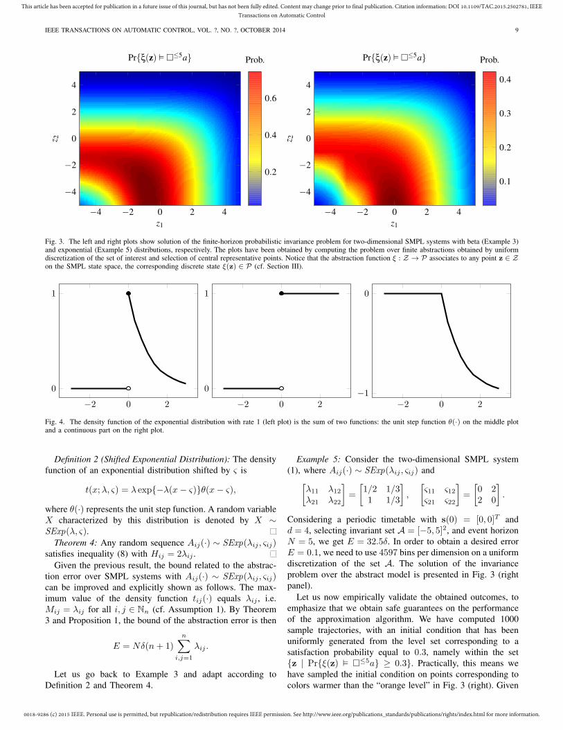
Considering a periodic timetable with s(0) = [0, 0]T andd = 4, selecting invariant set A = [−5, 5]2, and eventhorizon N = 5, according to Theorem 2 and Proposition1 we obtain an abstraction error E = 43.5δ. In order toobtain an abstraction error bounded by E = 0.1, we wouldneed to discretize set A uniformly with 6152 bins per eachdimension (step 1 of Algorithm 2). The representative pointshave been selected at the center of the squares obtainedby uniform discretization (step 2). The obtained finite-stateMC has m = 61522 + 1 discrete states (step 3), where theadditional state [30], [32] is considered as the representativepoint of the partition set Z\A. The solution of the invarianceproblem obtained over the abstract model (cf. Proposition 3) isdepicted in Fig. 3 (left panel). It is computed via the softwaretool FAUST2 [48], which is implemented in MATLAB andavailable for download.
C. Piecewise Lipschitz-Continuous Density Functions
The structural assumptions raised in Section IV-A limit thegeneral applicability of the work. For the sake of generality,we extend the previous results to models aligned with thefollowing requirement.
Assumption 3: The density functions tij(·) for i, j ∈ Nn arepiecewise Lipschitz-continuous, namely there exist partitionsR = ∪
mij
k=1Dkij and corresponding finite and positive constants
hkij , such that
|tkij(z)− tkij(z′)| ≤ hkij |z − z′| for all k ∈ Nmij
; z, z′ ∈ Dkij ,
tij(z) =
mij∑
k=1
tkij(z)1Dkij(z) for all z ∈ R.
This alternative assumption relaxes Assumption 2, allowingdiscontinuities in the density functions tij(·): this makes theresults applicable to a wider class of SMPL systems.
The notation k used in Assumption 3 does not denote apower, nor the occurrence index in (1), it is the index ofa set in the partition of cardinality
∑
i,j mij . Notice that ifAssumption 3 holds and the density functions are Lipschitz-continuous, then Assumption 2 is automatically satisfied withhij = maxk h
kij . In other words, with Assumption 3 we
allow relaxing Assumption 2 to hold only within arbitrary setspartitioning the state space of the SMPL system. For instance,as expected for the probabilistic invariance problem we maylimit the assumption to hold within the invariant set.
Under Assumptions 1 and 3, we now present a resultextending Theorem 2 for the computation of the constant H .
Theorem 3: Under Assumptions 1 and 3, the constant H inProposition 1 is
H =
n∑
i,j=1
Hij + (n− 1)Mij ,
where Hij = Li maxk hkij +
∑
k |Jkij | and Li = L(Πi(Z)).
The notation Jkij = limz↓ck
ijtij(z) − limz↑ck
ijtij(z) denotes
the jump distance of the density function tij(·) at the k-thdiscontinuity point ckij .The proof is similar to that of Theorem 2, the only differencebeing in the computation of constant Hij for the inequality
∫
Πi(Z)
|tij(zi−dij−zj)−tij(zi−dij−z′j)|dzi ≤ Hij |zj−z
′j |, (8)
for all zj , z′j ∈ Πj(Z), which utilizes a decomposition of tijinto a continuous part and a piecewise constant function. Thecomplete proof is presented in Appendix A. We display theresults with a numerical example.
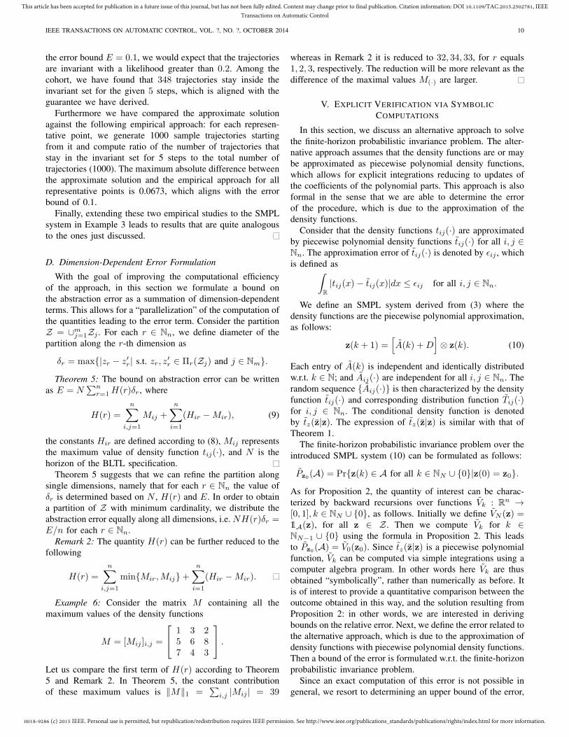
Example 4: Consider the density function of the exponentialdistribution with rate 1, i.e. t(z) = e−z if z ≥ 0 and 0otherwise (cf. Fig. 4 in the left). Notice that the densityfunction is piecewise Lipschitz-continuous (cf. Assumption 3).Furthermore the density function presents one discontinuitypoint c1 = 0 with associated jump distance equal to J1 = 1.One can show that the density function can be decomposedinto a piecewise constant function gd(z) = θ(z) and acontinuous function gc(z) = 01z<0 + (e−z − 1)1z≥0, asdepicted in Fig. 4 (middle and right plots).
In some cases, it is possible to obtain a smaller valuefor Hij by substituting the density function directly into theinequality in (8). Furthermore Hij may be independent of thesize of the state space. For instance, if the delay is modeledby an exponential distribution as in Example 1, then Aij(·)for all i, j ∈ Nn follows a shifted exponential distribution,i.e. Aij(·) ∼ SExp(λij , ςij). In this case, Hij = λij + λ2ijLi,as per Theorem 3. However if we compute directly the left-hand side of (8), we get the quantity Hij = 2λij , which isindependent of the shape of the state space. This fact is provenin general in Theorem 4, for the class of distribution functionsintroduced next.
0018-9286 (c) 2015 IEEE. Personal use is permitted, but republication/redistribution requires IEEE permission. See http://www.ieee.org/publications_standards/publications/rights/index.html for more information.
This article has been accepted for publication in a future issue of this journal, but has not been fully edited. Content may change prior to final publication. Citation information: DOI 10.1109/TAC.2015.2502781, IEEETransactions on Automatic Control
IEEE TRANSACTIONS ON AUTOMATIC CONTROL, VOL. ?, NO. ?, OCTOBER 2014 9
−4 −2 0 2 4
−4
−2
0
2
4
z1
z2
Pr{ξ(z) � �≤5
a}
0.2
0.4
0.6
Prob.
−4 −2 0 2 4
−4
−2
0
2
4
z1
z2
Pr{ξ(z) � �≤5
a}
0.1
0.2
0.3
0.4
Prob.
Fig. 3. The left and right plots show solution of the finite-horizon probabilistic invariance problem for two-dimensional SMPL systems with beta (Example 3)and exponential (Example 5) distributions, respectively. The plots have been obtained by computing the problem over finite abstractions obtained by uniformdiscretization of the set of interest and selection of central representative points. Notice that the abstraction function ξ : Z → P associates to any point z ∈ Zon the SMPL state space, the corresponding discrete state ξ(z) ∈ P (cf. Section III).
−2 0 2
0
1
−2 0 2
0
1
−2 0 2
−1
0
Fig. 4. The density function of the exponential distribution with rate 1 (left plot) is the sum of two functions: the unit step function θ(·) on the middle plotand a continuous part on the right plot.
Definition 2 (Shifted Exponential Distribution): The densityfunction of an exponential distribution shifted by ς is
t(x;λ, ς) = λ exp{−λ(x− ς)}θ(x− ς),
where θ(·) represents the unit step function. A random variableX characterized by this distribution is denoted by X ∼SExp(λ, ς).
Theorem 4: Any random sequence Aij(·) ∼ SExp(λij , ςij)satisfies inequality (8) with Hij = 2λij .
Given the previous result, the bound related to the abstrac-tion error over SMPL systems with Aij(·) ∼ SExp(λij , ςij)can be improved and explicitly shown as follows. The max-imum value of the density function tij(·) equals λij , i.e.Mij = λij for all i, j ∈ Nn (cf. Assumption 1). By Theorem3 and Proposition 1, the bound of the abstraction error is then
E = Nδ(n+ 1)n∑
i,j=1
λij .
Let us go back to Example 3 and adapt according toDefinition 2 and Theorem 4.
Example 5: Consider the two-dimensional SMPL system(1), where Aij(·) ∼ SExp(λij , ςij) and
[λ11 λ12λ21 λ22
]
=
[1/2 1/31 1/3
]
,
[ς11 ς12ς21 ς22
]
=
[0 22 0
]
.
Considering a periodic timetable with s(0) = [0, 0]T andd = 4, selecting invariant set A = [−5, 5]2, and event horizonN = 5, we get E = 32.5δ. In order to obtain a desired errorE = 0.1, we need to use 4597 bins per dimension on a uniformdiscretization of the set A. The solution of the invarianceproblem over the abstract model is presented in Fig. 3 (rightpanel).
Let us now empirically validate the obtained outcomes, toemphasize that we obtain safe guarantees on the performanceof the approximation algorithm. We have computed 1000sample trajectories, with an initial condition that has beenuniformly generated from the level set corresponding to asatisfaction probability equal to 0.3, namely within the set{z | Pr{ξ(z) � �
≤5a} ≥ 0.3}. Practically, this means wehave sampled the initial condition on points corresponding tocolors warmer than the “orange level” in Fig. 3 (right). Given
0018-9286 (c) 2015 IEEE. Personal use is permitted, but republication/redistribution requires IEEE permission. See http://www.ieee.org/publications_standards/publications/rights/index.html for more information.
This article has been accepted for publication in a future issue of this journal, but has not been fully edited. Content may change prior to final publication. Citation information: DOI 10.1109/TAC.2015.2502781, IEEETransactions on Automatic Control
IEEE TRANSACTIONS ON AUTOMATIC CONTROL, VOL. ?, NO. ?, OCTOBER 2014 10
the error bound E = 0.1, we would expect that the trajectoriesare invariant with a likelihood greater than 0.2. Among thecohort, we have found that 348 trajectories stay inside theinvariant set for the given 5 steps, which is aligned with theguarantee we have derived.
Furthermore we have compared the approximate solutionagainst the following empirical approach: for each represen-tative point, we generate 1000 sample trajectories startingfrom it and compute ratio of the number of trajectories thatstay in the invariant set for 5 steps to the total number oftrajectories (1000). The maximum absolute difference betweenthe approximate solution and the empirical approach for allrepresentative points is 0.0673, which aligns with the errorbound of 0.1.
Finally, extending these two empirical studies to the SMPLsystem in Example 3 leads to results that are quite analogousto the ones just discussed.
D. Dimension-Dependent Error Formulation
With the goal of improving the computational efficiencyof the approach, in this section we formulate a bound onthe abstraction error as a summation of dimension-dependentterms. This allows for a “parallelization” of the computation ofthe quantities leading to the error term. Consider the partitionZ = ∪m
j=1Zj . For each r ∈ Nn, we define diameter of thepartition along the r-th dimension as
δr = max{|zr − z′r| s.t. zr, z′r ∈ Πr(Zj) and j ∈ Nm}.
Theorem 5: The bound on abstraction error can be writtenas E = N
∑nr=1H(r)δr, where
H(r) =
n∑
i,j=1
Mij +
n∑
i=1
(Hir −Mir), (9)
the constants Hir are defined according to (8), Mij representsthe maximum value of density function tij(·), and N is thehorizon of the BLTL specification.
Theorem 5 suggests that we can refine the partition alongsingle dimensions, namely that for each r ∈ Nn the value ofδr is determined based on N , H(r) and E. In order to obtaina partition of Z with minimum cardinality, we distribute theabstraction error equally along all dimensions, i.e. NH(r)δr =E/n for each r ∈ Nn.
Remark 2: The quantity H(r) can be further reduced to thefollowing
H(r) =
n∑
i,j=1
min{Mir,Mij}+n∑
i=1
(Hir −Mir).
Example 6: Consider the matrix M containing all themaximum values of the density functions
M = [Mij ]i,j =
1 3 25 6 87 4 3
.
Let us compare the first term of H(r) according to Theorem5 and Remark 2. In Theorem 5, the constant contributionof these maximum values is ‖M‖1 =
∑
i,j |Mij | = 39
whereas in Remark 2 it is reduced to 32, 34, 33, for r equals1, 2, 3, respectively. The reduction will be more relevant as thedifference of the maximal values M(·) are larger.
V. EXPLICIT VERIFICATION VIA SYMBOLIC
COMPUTATIONS
In this section, we discuss an alternative approach to solvethe finite-horizon probabilistic invariance problem. The alter-native approach assumes that the density functions are or maybe approximated as piecewise polynomial density functions,which allows for explicit integrations reducing to updates ofthe coefficients of the polynomial parts. This approach is alsoformal in the sense that we are able to determine the errorof the procedure, which is due to the approximation of thedensity functions.
Consider that the density functions tij(·) are approximatedby piecewise polynomial density functions tij(·) for all i, j ∈Nn. The approximation error of tij(·) is denoted by ǫij , whichis defined as
∫
R
|tij(x)− tij(x)|dx ≤ ǫij for all i, j ∈ Nn.
We define an SMPL system derived from (3) where thedensity functions are the piecewise polynomial approximation,as follows:
z(k + 1) =[
A(k) +D]
⊗ z(k). (10)
Each entry of A(k) is independent and identically distributedw.r.t. k ∈ N; and Aij(·) are independent for all i, j ∈ Nn. Therandom sequence {Aij(·)} is then characterized by the densityfunction tij(·) and corresponding distribution function Tij(·)for i, j ∈ Nn. The conditional density function is denotedby tz(z|z). The expression of tz(z|z) is similar with that ofTheorem 1.
The finite-horizon probabilistic invariance problem over theintroduced SMPL system (10) can be formulated as follows:
Pz0(A) = Pr{z(k) ∈ A for all k ∈ NN ∪ {0}|z(0) = z0}.
As for Proposition 2, the quantity of interest can be charac-terized by backward recursions over functions Vk : R
n →[0, 1], k ∈ NN ∪ {0}, as follows. Initially we define VN (z) =1A(z), for all z ∈ Z . Then we compute Vk for k ∈NN−1 ∪ {0} using the formula in Proposition 2. This leadsto Pz0
(A) = V0(z0). Since tz(z|z) is a piecewise polynomialfunction, Vk can be computed via simple integrations using acomputer algebra program. In other words here Vk are thusobtained “symbolically”, rather than numerically as before. Itis of interest to provide a quantitative comparison between theoutcome obtained in this way, and the solution resulting fromProposition 2: in other words, we are interested in derivingbounds on the relative error. Next, we define the error related tothe alternative approach, which is due to the approximation ofdensity functions with piecewise polynomial density functions.Then a bound of the error is formulated w.r.t. the finite-horizonprobabilistic invariance problem.
Since an exact computation of this error is not possible ingeneral, we resort to determining an upper bound of the error,
0018-9286 (c) 2015 IEEE. Personal use is permitted, but republication/redistribution requires IEEE permission. See http://www.ieee.org/publications_standards/publications/rights/index.html for more information.
This article has been accepted for publication in a future issue of this journal, but has not been fully edited. Content may change prior to final publication. Citation information: DOI 10.1109/TAC.2015.2502781, IEEETransactions on Automatic Control
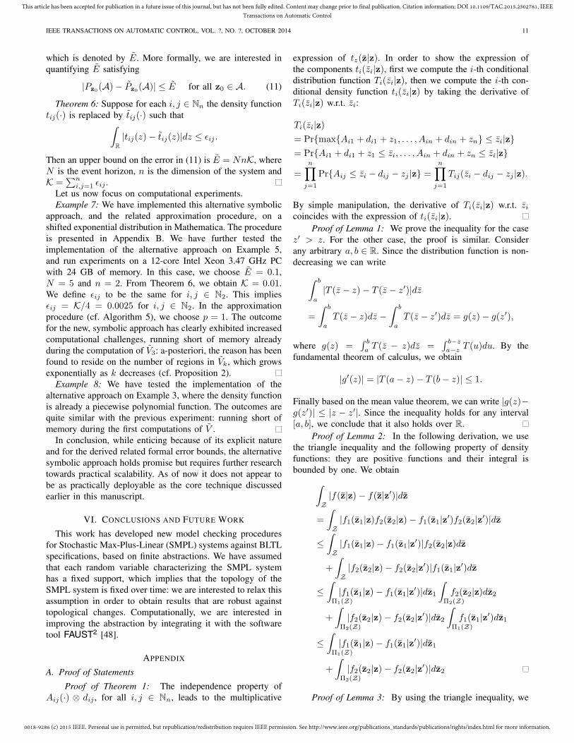
IEEE TRANSACTIONS ON AUTOMATIC CONTROL, VOL. ?, NO. ?, OCTOBER 2014 11
which is denoted by E. More formally, we are interested inquantifying E satisfying
|Pz0(A)− Pz0
(A)| ≤ E for all z0 ∈ A. (11)
Theorem 6: Suppose for each i, j ∈ Nn the density functiontij(·) is replaced by tij(·) such that
∫
R
|tij(z)− tij(z)|dz ≤ ǫij .
Then an upper bound on the error in (11) is E = NnK, whereN is the event horizon, n is the dimension of the system andK =
∑ni,j=1 ǫij .
Let us now focus on computational experiments.Example 7: We have implemented this alternative symbolic
approach, and the related approximation procedure, on ashifted exponential distribution in Mathematica. The procedureis presented in Appendix B. We have further tested theimplementation of the alternative approach on Example 5,and run experiments on a 12-core Intel Xeon 3.47 GHz PCwith 24 GB of memory. In this case, we choose E = 0.1,N = 5 and n = 2. From Theorem 6, we obtain K = 0.01.We define ǫij to be the same for i, j ∈ N2. This impliesǫij = K/4 = 0.0025 for i, j ∈ N2. In the approximationprocedure (cf. Algorithm 5), we choose p = 1. The outcomefor the new, symbolic approach has clearly exhibited increasedcomputational challenges, running short of memory alreadyduring the computation of V3: a-posteriori, the reason has beenfound to reside on the number of regions in Vk, which growsexponentially as k decreases (cf. Proposition 2).
Example 8: We have tested the implementation of thealternative approach on Example 3, where the density functionis already a piecewise polynomial function. The outcomes arequite similar with the previous experiment: running short ofmemory during the first computations of V .
In conclusion, while enticing because of its explicit natureand for the derived related formal error bounds, the alternativesymbolic approach holds promise but requires further researchtowards practical scalability. As of now it does not appear tobe as practically deployable as the core technique discussedearlier in this manuscript.
VI. CONCLUSIONS AND FUTURE WORK
This work has developed new model checking proceduresfor Stochastic Max-Plus-Linear (SMPL) systems against BLTLspecifications, based on finite abstractions. We have assumedthat each random variable characterizing the SMPL systemhas a fixed support, which implies that the topology of theSMPL system is fixed over time: we are interested to relax thisassumption in order to obtain results that are robust againsttopological changes. Computationally, we are interested inimproving the abstraction by integrating it with the softwaretool FAUST2 [48].
APPENDIX
A. Proof of Statements
Proof of Theorem 1: The independence property ofAij(·) ⊗ dij , for all i, j ∈ Nn, leads to the multiplicative
expression of tz(z|z). In order to show the expression ofthe components ti(zi|z), first we compute the i-th conditionaldistribution function Ti(zi|z), then we compute the i-th con-ditional density function ti(zi|z) by taking the derivative ofTi(zi|z) w.r.t. zi:
Ti(zi|z)
= Pr{max{Ai1 + di1 + z1, . . . , Ain + din + zn} ≤ zi|z}
= Pr{Ai1 + di1 + z1 ≤ zi, . . . , Ain + din + zn ≤ zi|z}
=
n∏
j=1
Pr{Aij ≤ zi − dij − zj |z} =
n∏
j=1
Tij(zi − dij − zj |z).
By simple manipulation, the derivative of Ti(zi|z) w.r.t. zicoincides with the expression of ti(zi|z).
Proof of Lemma 1: We prove the inequality for the casez′ > z. For the other case, the proof is similar. Considerany arbitrary a, b ∈ R. Since the distribution function is non-decreasing we can write
∫ b
a
|T (z − z)− T (z − z′)|dz
=
∫ b
a
T (z − z)dz −
∫ b
a
T (z − z′)dz = g(z)− g(z′),
where g(z) =∫ b
aT (z − z)dz =
∫ b−z
a−zT (u)du. By the
fundamental theorem of calculus, we obtain
|g′(z)| = |T (a− z)− T (b− z)| ≤ 1.
Finally based on the mean value theorem, we can write |g(z)−g(z′)| ≤ |z − z′|. Since the inequality holds for any interval[a, b], we conclude that it also holds over R.
Proof of Lemma 2: In the following derivation, we usethe triangle inequality and the following property of densityfunctions: they are positive functions and their integral isbounded by one. We obtain
∫
Z
|f(z|z)− f(z|z′)|dz
=
∫
Z
|f1(z1|z)f2(z2|z)− f1(z1|z′)f2(z2|z
′)|dz
≤
∫
Z
|f1(z1|z)− f1(z1|z′)|f2(z2|z)dz
+
∫
Z
|f2(z2|z)− f2(z2|z′)|f1(z1|z
′)dz
≤
∫
Π1(Z)
|f1(z1|z)− f1(z1|z′)|dz1
∫
Π2(Z)
f2(z2|z)dz2
+
∫
Π2(Z)
|f2(z2|z)− f2(z2|z′)|dz2
∫
Π1(Z)
f1(z1|z′)dz1
≤
∫
Π1(Z)
|f1(z1|z)− f1(z1|z′)|dz1
+
∫
Π2(Z)
|f2(z2|z)− f2(z2|z′)|dz2
Proof of Lemma 3: By using the triangle inequality, we
0018-9286 (c) 2015 IEEE. Personal use is permitted, but republication/redistribution requires IEEE permission. See http://www.ieee.org/publications_standards/publications/rights/index.html for more information.
This article has been accepted for publication in a future issue of this journal, but has not been fully edited. Content may change prior to final publication. Citation information: DOI 10.1109/TAC.2015.2502781, IEEETransactions on Automatic Control
IEEE TRANSACTIONS ON AUTOMATIC CONTROL, VOL. ?, NO. ?, OCTOBER 2014 12
obtain the following chain of inequalities∫
C
|f(z|z1, z2)− f(z|z′1, z′2)|dz
=
∫
C
|f1(z, z1)f2(z, z2)− f1(z, z′1)f2(z, z
′2)|dz
≤
∫
C
|f1(z, z1)− f1(z, z′1)|f2(z, z2)dz
+
∫
C
|f2(z, z2)− f2(z, z′2)|f1(z, z
′1)dz
≤M2
∫
C
|f1(z, z1)− f1(z, z′1)|dz
+M1
∫
C
|f2(z, z2)− f2(z, z′2)|dz.
Proof of Theorem 2: Using Lemma 2 on the multiplica-tive structure of the conditional density function we have:∫
Z
|tz(z|z)− tz(z|z′)|dz ≤
n∑
i=1
∫
Πi(Z)
|ti(zi|z)− ti(zi|z′)|dzi,
and employing the triangle inequality for the additive structureof ti(zi|z) and utilizing Lemma 3 and Assumption 1, weobtain:
≤n∑
i,j=1
∫
Πi(Z)
|tij(zi − dij − zj)− tij(zi − dij − z′j)|dzi
+
n∑
i,j=1
n∑
k=1k 6=j
Mij
∫
Πi(Z)
|Tik(zi − dik − zk) (12)
−Tik(zi − dik − z′k)|dzi.
Finally, by Assumption 2 and Lemma 1 we obtain
≤n∑
i,j=1
hijL(Πi(Z))|zj − z′j |+n∑
i,j=1
n∑
k=1k 6=j
Mij |zk − z′k|
≤
n∑
i,j=1
Hij + (n− 1)Mij
‖z− z′‖ = H‖z− z
′‖.
Proof of Theorem 3: We show that the constant Hij in(8) exists for piecewise Lipschitz-continuous density functionsand compute it based on Assumption 3. Introduce the twofunctions gdij(z) =
∑mij−1k=1 J k
ijθ(z − ckij) and gcij(z) =
tij(z)− gdij(z), where J kij =
∑kq=1 J
qij , θ(·) denotes the unit
step function, and {ckij | k ∈ Nmij−1} are the discontinuitypoints of the density function tij(·). Then the density functionis decomposed into tij(z) = gcij(z) + gdij(z), where gcij isits continuous part and gdij is a piecewise constant functionencompassing its jumps (cf. Fig. 4). It is clear that
∫
Πi(Z)
|gdij(z − dij − z)− gdij(z − dij − z′)|dz
≤m−1∑
k=1
|J kij ||z − z′|,
∫
Πi(Z)
|gcij(z − dij − z)− gcij(z − dij − z′)|dz
≤ Li maxk
hkij |z − z′|.
Adding both sides using the triangle inequality leads to thedesired value for Hij .
Proof of Theorem 4: We will show that the followinginequality holds:∫
Πi(A)
|tij(zi − dij − zj ;λij , ςij)− tij(zi − dij − z′j ;λij , ςij)|dzi
≤ 2λij |zj − z′j |, for all zj , z′j ∈ Πj(Z).
Without loss of generality, since the integrand and theexpression on the right-hand side are symmetric w.r.t. zj andz′j , let us assume that zj ≤ z′j . It follows that the integrand isa piecewise continuous function of zi, zj , z′j :
λij exp{−λij(zi − dij − z′j − ςij)}−λij exp{−λij(zi − dij − zj − ςij)},
if zi ≥ z′j + dij + ςij ,λij exp{−λij(zi − dij − zj − ςij)},
if zj + dij + ςij ≤ zi ≤ z′j + dij + ςij ,0, if zi ≤ zj + dij + ςij .
Thus the overall bounds can be computed based on the boundsof the first two sub-functions. We will prove that the first twosub-functions are bounded by λij |zj−z′j |. Let us focus on thefirst sub-function:
λij
∫ +∞
z′
j+dij+ςij
(exp{−λij(zi − dij − z′j − ςij)}
− exp{−λij(zi − dij − zj − ςij)}) dzi
= λij(exp{λijz′j} − exp{λijzj})
∫ +∞
z′
j+dij+ςij
exp{−λij(zi − dij − ςij)}dzi
= (exp{λijz′j} − exp{λijzj}) exp{−λijz
′j}
= 1− exp{−λij(z′j − zj)}
≤ λij |zj − z′j |.
The last inequality holds because λij(z′j − zj) ≥ 0 and 1 −exp{−z} ≤ z for all z ≥ 0. Then we continue to the secondsub-function:
λij
∫ z′
j+dij+ςij
zj+dij+ςij
exp{−λij(zi − dij − zj − ςij)}dzi
= − exp{−λij(z′j − zj)}+ 1
≤ λij |zj − z′j |.
Proof of Theorem 5: The proof follows the same line ofproofs of Theorems 2 and 3. We utilize the inequality (8) andLemma 1 in the right-hand side of (12) to get
∫
Z
|tz(z|z)− tz(z|z′)|dz ≤
n∑
i,j=1
Hijδj +n∑
i,j=1
n∑
k=1k 6=j
Mijδk,
which is equal to∑n
r=1H(r)δr with H(r) defined in (9).Finally, Proposition 1 guarantees the abstraction error of E =N
∑nr=1H(r)δr.

0018-9286 (c) 2015 IEEE. Personal use is permitted, but republication/redistribution requires IEEE permission. See http://www.ieee.org/publications_standards/publications/rights/index.html for more information.
This article has been accepted for publication in a future issue of this journal, but has not been fully edited. Content may change prior to final publication. Citation information: DOI 10.1109/TAC.2015.2502781, IEEETransactions on Automatic Control
IEEE TRANSACTIONS ON AUTOMATIC CONTROL, VOL. ?, NO. ?, OCTOBER 2014 13
Proof of Theorem 6: We consider Tij(·) and Tij(·) theassociated distribution functions:
|Tij(z)− Tij(z)| =
∣∣∣∣
∫ z
−∞
tij(u)du−
∫ z
−∞
tij(u)du
∣∣∣∣
≤
∫ z
−∞
|tij(u)− tij(u)|du ≤ ǫij .
Using this inequality we obtain∫
Z
|tz(z|z)− tz(z|z)|dz ≤n∑
i=1
∫
Πi(Z)
|ti(zi|z)− ti(zi|z)|dzi
≤n∑
i,j=1
∫
Πi(Z)
|tij(zi + d− zj)− tij(zi + d− zj)|dzi
+n∑
i,j=1
n∑
k=1k 6=j
supzi,zk
|Tik(zi + d− zk)− Tik(zi + d− zk)|
≤n∑
i,j=1
ǫij +n∑
i,j=1
n∑
k=1k 6=j
ǫik = nn∑
i,j=1
ǫij .
The upper bound on the error E is obtained by applying theresult in [35, Lemma 1] to the preceding inequality.
B. Approximation of Exponential Functions by PiecewisePolynomial Functions
We now develop a procedure to compute an approximationof exponential functions with arbitrary accuracy. The approx-imation is characterized by a piecewise polynomial function.
Here we consider the negative exponential function f :[0,+∞) → [0, 1], x 7→ e−x and provide a piecewise poly-nomial approximation f : [0,+∞) → R such that
∫ +∞
0
|f(x)− f(x)|dx ≤ ǫ,
for any given threshold ǫ > 0. Having this piecewise polyno-mial approximation of the negative exponential function andusing shifted scaled variables, we can approximate any shiftedexponential distribution by a piecewise polynomial one for agiven threshold.
For this purpose we select the shifted Legendre polynomialsas the basis function with the following explicit representation
Pn(x) = (−1)nn∑
k=0
(nk
)(n+ kk
)
(−x)k,
which are orthogonal in the interval [0, 1], i.e.∫ 1
0
Pm(x)Pn(x)dx =1
2n+ 1δmn,
where δmn is the Kronecker delta, which equals 1 if m = nand 0 otherwise. Note that since we do not have any weightingfunction inside the integral, we need to select the basisfunctions to be orthogonal with weight 1. To the best ofour knowledge, Legendre polynomials are the only availableoption.
Define the new basis functions ψij(x) and construct f(x)according to
ψij(x) = Pj
(x− iℓ
ℓ
)
1[iℓ,(i+1)ℓ)(x),
f(x) =
p−1∑
i=0
qi∑
j=0
cijψij(x),
where 1[iℓ,(i+1)ℓ)(·) is the indicator function of the interval[iℓ, (i+ 1)ℓ), the number of intervals for the function f(·) isdenoted by p, the maximum degree of basis polynomials in thei-th interval is denoted by qi, and the length of intervals ℓ > 0will be specified later. Note that these basis functions are stillorthogonal over R and the coefficients can be computed as
cij = e−iℓ (2j + 1)
∫ 1
0
e−ℓuPj(u)du
︸ ︷︷ ︸
αj
.
In the above equation, observe that αj does not depend on i.This observation makes it possible to take q0 = q1 = . . . =qp−1 = q and simplify the function f(·) by the following
fq(x) =
q∑
j=0
αjPj(x),
f(x) =
p−1∑
i=0
e−iℓfq
(x− iℓ
ℓ
)
1[iℓ,(i+1)ℓ)(x).
Remark 3: The coefficients have a closed form
αj = (2j + 1)
j∑
k=0
(−1)j+k
(jk
)(j + kk
)k!
ℓk+1
− (2j + 1)e−ℓ
j∑
k=0
k∑
r=0
(−1)j+k
(jk
)(j + kk
)
k!
(k − r)!
1
ℓr+1.
Algorithm 5 presents the required steps to construct theapproximation function. The advantage of this algorithm isthat we compute the polynomial only for one interval and useit to generate the polynomials for all intervals. This propertyis due to the characteristics of the exponential function and ingeneral does not hold for other functions.
Theorem 7: If q ∈ N is selected sufficiently large such that∫ 1
0
|e−ℓx − fq(x)|dx ≤ ǫ1, (13)
then f(x) approximates the exponential function f(x) = e−x
which satisfies the inequality∫ +∞
0|f(x)− f(x)|dx ≤ ǫ.
Remark 4: The completeness of Legendre polynomials asbasis functions implies that
+∞∑
j=0
α2j
2j + 1=
∫ 1
0
e−2ℓudu =1− e−2ℓ
2ℓ.
Moreover it guarantees that
limq→∞
∫ 1
0
|e−ℓx − fq(x)|dx = 0.
0018-9286 (c) 2015 IEEE. Personal use is permitted, but republication/redistribution requires IEEE permission. See http://www.ieee.org/publications_standards/publications/rights/index.html for more information.
This article has been accepted for publication in a future issue of this journal, but has not been fully edited. Content may change prior to final publication. Citation information: DOI 10.1109/TAC.2015.2502781, IEEETransactions on Automatic Control
IEEE TRANSACTIONS ON AUTOMATIC CONTROL, VOL. ?, NO. ?, OCTOBER 2014 14
input: The approximation precision 0 < ǫ < 1 and thenumber of intervals p ∈ N
output: f(x) =p−1∑
i=0
e−iℓfq(x−iℓℓ
)1[iℓ,(i+1)ℓ)(x)
1: Select the length of intervals ℓ = − 1p ln
(ǫ2
)> 0
2: Compute ǫ1 =ǫ
2ℓ
1− e−ℓ
1− e−pℓ
3: Define fq : [0, 1] → R as the polynomial approximationof the function e−ℓx in the interval [0, 1]:
fq(x) =
q∑
j=0
αjPj(x), αj = (2j + 1)
∫ 1
0
e−ℓuPj(u)du.
4: Select q sufficiently large such that∫ 1
0
|e−ℓx − fq(x)|dx ≤ ǫ1.
Fig. 5. Algorithm 5. Approximation of the function f(x) = e−x by apiecewise polynomial function f : [0,+∞) → R.
Then there exists a q such that the inequality (13) is satisfied.The convergence to zero is not monotonic but we can findan upper bound for the quantity of q using Cauchy-Schwarzinequality:
∫ 1
0
|e−ℓx − fq(x)|dx ≤
[∫ 1
0
(e−ℓx − fq(x))2dx
]1/2
=
1− e−2ℓ
2ℓ−
q∑
j=0
α2j
2j + 1
1/2
.
The right-hand side is now monotonically converges to zerowhich can be used to find an upper bound for the smallestvalue of q satisfying (13) (cf. step 4 of Algorithm 5). Thisupper bound must satisfy the inequality
q∑
j=0
α2j
2j + 1≥
1− e−2ℓ
2ℓ− ǫ21.
REFERENCES
[1] F. Baccelli, G. Cohen, and B. Gaujal, “Recursive equations and basicproperties of timed Petri nets,” Discrete Event Dynamic Systems: Theoryand Applications, vol. 1, no. 4, pp. 415–439, Jun. 1992.
[2] H. P. Hillion and J. P. Proth, “Performance evaluation of job-shopsystems using timed event graphs,” IEEE Trans. Autom. Control, vol. 34,no. 1, pp. 3–9, Jan. 1989.
[3] B. Heidergott, G. J. Olsder, and J. W. van der Woude, Max Plus atWork–Modeling and Analysis of Synchronized Systems: A Course onMax-Plus Algebra and Its Applications. Princeton University Press,2006.
[4] B. J. P. Roset, H. Nijmeijer, J. A. W. M. van Eekelen, E. Lefeber,and J. E. Rooda, “Event driven manufacturing systems as time domaincontrol systems,” in Proc. 44th IEEE Conf. Decision and Control andEuropean Control Conf. (CDC-ECC’05), Dec. 2005, pp. 446–451.
[5] J. A. W. M. van Eekelen, E. Lefeber, and J. E. Rooda, “Coupling eventdomain and time domain models of manufacturing systems,” in Proc.45th IEEE Conf. Decision and Control (CDC’06), Dec. 2006, pp. 6068–6073.
[6] B. Heidergott, Max-Plus Linear Stochastic Systems and PerturbationAnalysis (The International Series on Discrete Event Dynamic Systems).Secaucus, NJ: Springer-Verlag New York, Inc., 2006.
[7] G. J. Olsder, J. A. C. Resing, R. E. de Vries, M. S. Keane, andG. Hooghiemstra, “Discrete event systems with stochastic processingtimes,” IEEE Trans. Autom. Control, vol. 35, no. 3, pp. 299–302, Mar.1990.
[8] J. A. C. Resing, R. E. de Vries, G. Hooghiemstra, M. S. Keane, andG. J. Olsder, “Asymptotic behavior of random discrete event systems,”Stochastic Processes and their Applications, vol. 36, no. 2, pp. 195–216,Dec. 1990.
[9] J. W. van der Woude and B. Heidergott, “Asymptotic growth rateof stochastic max-plus systems that with a positive probability havea sunflower-like support,” in Proc. 8th Int. Workshop Discrete EventSystems (WODES’06), Jul. 2006, pp. 451–456.
[10] R. M. P. Goverde, B. Heidergott, and G. Merlet, “A coupling approachto estimating the Lyapunov exponent of stochastic max-plus linearsystems,” European Journal of Operational Research, vol. 210, no. 2,pp. 249–257, 2011.
[11] F. Baccelli, G. Cohen, G. J. Olsder, and J.-P. Quadrat, Synchronizationand Linearity, An Algebra for Discrete Event Systems. John Wiley andSons, 1992.
[12] F. Baccelli and D. Hong, “Analytic expansions of max-plus Lyapunovexponents,” The Annals of Applied Probability, vol. 10, no. 3, pp. 779–827, Aug. 2000.
[13] S. Gaubert and D. Hong, “Series expansions of Lyapunov exponentsand forgetful monoids,” INRIA, Tech. Rep. RR-3971, Jul. 2000.
[14] G. Merlet, “Cycle time of stochastic max-plus linear systems.” ElectronicJournal of Probability, vol. 13, no. 12, pp. 322–340, 2008.
[15] S. Farahani, T. J. J. van den Boom, H. van der Weide, and B. De Schutter,“An approximation approach for model predictive control of stochasticmax-plus linear systems,” in Proc. 10th Int. Workshop Discrete EventSystems (WODES’10), Berlin, DE, Aug./Sep. 2010, pp. 386–391.
[16] S. Farahani, T. J. J. van den Boom, and B. De Schutter, “Exactand approximate approaches to the identification of stochastic max-plus-linear systems,” Discrete Event Dynamic Systems: Theory andApplications, pp. 1–25, Apr. 2013.
[17] K. Cechlarova and R. A. Cuninghame-Green, “Interval systems of max-separable linear equations,” Linear Algebra and its Applications, vol.340, no. 1-3, pp. 215–224, 2002.
[18] K. Cechlarova, “Eigenvectors of interval matrices over maxplus algebra,”Discrete Applied Mathematics, vol. 150, no. 1-3, pp. 2–15, 2005.
[19] H. Myskova, “Interval systems of max-separable linear equations,”Linear Algebra and its Applications, vol. 403, no. 0, pp. 263–272, 2005.
[20] D. Adzkiya, B. De Schutter, and A. Abate, “Finite abstractions of max-plus-linear systems,” IEEE Trans. Autom. Control, vol. 58, no. 12, pp.3039–3053, Dec. 2013.
[21] R. P. Kurshan, Computer-Aided Verification of Coordinating Processes:The Automata-Theoretic Approach, ser. Princeton Series in ComputerScience. Princeton University Press, 1994.
[22] C. Baier, J.-P. Katoen, and H. Hermanns, “Approximate symbolic modelchecking of continous-time Markov chains,” in Proc. 10th Int. Conf.Concurrency Theory (CONCUR’99), ser. Lecture Notes in ComputerScience, J. C. M. Baeten and S. Mauw, Eds. Springer, Heidelberg,1999, vol. 1664, pp. 146–162.
[23] M. Kwiatkowska, G. Norman, R. Segala, and J. Sproston, “Verifyingquantitative properties of continuous probabilistic timed automata,” inProc. 11th Int. Conf. Concurrency Theory (CONCUR’00), ser. LectureNotes in Computer Science, C. Palamidessi, Ed. Springer, Heidelberg,2000, vol. 1877, pp. 123–137.
[24] R. Alur and D. L. Dill, “A theory of timed automata,” TheoreticalComputer Science, vol. 126, no. 2, pp. 183–235, 1994.
[25] H. J. Kushner and P. G. Dupuis, Numerical Methods for StochasticControl Problems in Continuous Time. New York: Springer-Verlag,2001.
[26] P. Chaput, V. Danos, P. Panangaden, and G. Plotkin, “ApproximatingMarkov processes by averaging,” Journal of the ACM, vol. 61, no. 1,pp. 5:1–5:45, Jan. 2014.
[27] K. Koutsoukos and D. Riley, “Computational methods for reachabilityanalysis of stochastic hybrid systems,” in Hybrid Systems: Computationand Control (HSCC’06), ser. Lecture Notes in Computer Science,J. Hespanha and A. Tiwari, Eds. Springer, Heidelberg, 2006, vol. 3927,pp. 377–391.
[28] M. Prandini and J. Hu, “Stochastic reachability: Theory and numericalapproximation,” in Stochastic hybrid systems, ser. Automation andControl Engineering Series 24, C. G. Cassandras and J. Lygeros, Eds.Taylor & Francis Group/CRC Press, 2006, pp. 107–138.
[29] A. Abate, M. Prandini, J. Lygeros, and S. Sastry, “Probabilistic reacha-bility and safety for controlled discrete time stochastic hybrid systems,”Automatica, vol. 44, no. 11, pp. 2724–2734, 2008.

0018-9286 (c) 2015 IEEE. Personal use is permitted, but republication/redistribution requires IEEE permission. See http://www.ieee.org/publications_standards/publications/rights/index.html for more information.
This article has been accepted for publication in a future issue of this journal, but has not been fully edited. Content may change prior to final publication. Citation information: DOI 10.1109/TAC.2015.2502781, IEEETransactions on Automatic Control
IEEE TRANSACTIONS ON AUTOMATIC CONTROL, VOL. ?, NO. ?, OCTOBER 2014 15
[30] A. Abate, J.-P. Katoen, J. Lygeros, and M. Prandini, “Approximate modelchecking of stochastic hybrid systems,” European Journal of Control,vol. 16, no. 6, pp. 624–641, 2010.
[31] S. Esmaeil Zadeh Soudjani and A. Abate, “Adaptive gridding forabstraction and verification of stochastic hybrid systems,” in Proc. 8thInt. Conf. Quantitative Evaluation of Systems (QEST’11), Sep. 2011, pp.59–69.
[32] ——, “Adaptive and sequential gridding procedures for the abstractionand verification of stochastic processes,” SIAM Journal on AppliedDynamical Systems, vol. 12, no. 2, pp. 921–956, 2013.
[33] ——, “Higher-order approximations for verification of stochastic hybridsystems,” in Automated Technology for Verification and Analysis, ser.Lecture Notes in Computer Science, S. Chakraborty and M. Mukund,Eds. Springer Verlag, Berlin Heidelberg, 2012, vol. 7561, pp. 416–434.
[34] S. Esmaeil Zadeh Soudjani, A. Abate, and R. Majumdar, “DynamicBayesian networks as formal abstractions of structured stochastic pro-cesses,” in 26th Int. Conf. Concurrency Theory (CONCUR’15), ser.Leibniz International Proceedings in Informatics (LIPIcs), L. Aceto andD. Frutos-Escrig, Eds., vol. 42, Dagstuhl, DE, 2015, pp. 169–183.
[35] I. Tkachev and A. Abate, “Formula-free finite abstractions for lineartemporal verification of stochastic hybrid systems,” in Hybrid Systems:Computation and Control (HSCC’13). ACM, 2013, pp. 283–292.
[36] A. Abate, “Approximation metrics based on probabilistic bisimulationsfor general state-space Markov processes: a survey,” Electronic Notes inTheoretical Computer Sciences, pp. 3–25, 2014.
[37] J. Desharnais, A. Edalat, and P. Panangaden, “Bisimulation for labelledMarkov processes,” Information and Computation, vol. 179, no. 2, pp.163 – 193, 2002.
[38] S. K. Jha, E. M. Clarke, C. J. Langmead, A. Legay, A. Platzer,and P. Zuliani, “A Bayesian approach to model checking biologicalsystems,” in Computational Methods in Systems Biology, ser. LectureNotes in Computer Science, P. Degano and R. Gorrieri, Eds. Springer,Heidelberg, 2009, vol. 5688, pp. 218–234.
[39] M. Rungger, M. Mazo, Jr., and P. Tabuada, “Specification-guidedcontroller synthesis for linear systems and safe linear-time temporallogic,” in Hybrid Systems: Computation and Control (HSCC’13), 2013,pp. 333–342.
[40] M. B. Horowitz, E. M. Wolff, and R. M. Murray, “A compositionalapproach to stochastic optimal control with co-safe temporal logicspecifications,” in IEEE/RSJ International Conference on IntelligentRobots and Systems (IROS’14), Sep. 2014, pp. 1466–1473.
[41] P. Zuliani, A. Platzer, and E. M. Clarke, “Bayesian statistical modelchecking with application to stateflow/simulink verification,” FormalMethods in System Design, vol. 43, no. 2, pp. 338–367, 2013.
[42] X. Ding, S. L. Smith, C. Belta, and D. Rus, “Optimal control of Markovdecision processes with linear temporal logic constraints,” IEEE Trans.Autom. Control, vol. 59, no. 5, pp. 1244–1257, May 2014.
[43] M. Kwiatkowska, G. Norman, and D. Parker, “PRISM 4.0: Verificationof probabilistic real-time systems,” in Proc. 23rd Int. Conf. ComputerAided Verification (CAV’11), ser. Lecture Notes in Computer Science,G. Gopalakrishnan and S. Qadeer, Eds., vol. 6806. Springer, Heidelberg,2011, pp. 585–591.
[44] J.-P. Katoen, M. Khattri, and I. S. Zapreev, “A Markov reward modelchecker,” in Proc. 2nd Int. Conf. Quantitative Evaluation of Systems(QEST’05). Los Alamos, CA, USA: IEEE Computer Society, 2005,pp. 243–244.
[45] D. Adzkiya, S. Esmaeil Zadeh Soudjani, and A. Abate, “Finite ab-stractions of stochastic max-plus-linear systems,” in Proc. 11th Int.Conf. Quantitative Evaluation of Systems (QEST’14), ser. Lecture Notesin Computer Science, G. Norman and W. Sanders, Eds. SpringerInternational Publishing, 2014, vol. 8657, pp. 74–89.
[46] R. M. P. Goverde, “Railway timetable stability analysis using max-plus system theory,” Transportation Research Part B: Methodological,vol. 41, no. 2, pp. 179–201, 2007.
[47] C. Baier and J.-P. Katoen, Principles of Model Checking. The MITPress, 2008.
[48] S. Esmaeil Zadeh Soudjani, C. Gevaerts, and A. Abate, “FAUST2: For-mal abstractions of uncountable-state stochastic processes,” in Tools andAlgorithms for the Construction and Analysis of Systems (TACAS’15),ser. Lecture Notes in Computer Science, C. Baier and C. Tinelli, Eds.Springer, Heidelberg, 2015, vol. 9035, pp. 272–286.
[49] S. Esmaeil Zadeh Soudjani and A. Abate, “Precise approximations ofthe probability distribution of a Markov process in time: an applicationto probabilistic invariance,” in Tools and Algorithms for the Constructionand Analysis of Systems (TACAS’14), ser. Lecture Notes in ComputerScience, E. Abraham and K. Havelund, Eds. Springer, Heidelberg,2014, vol. 8413, pp. 547–561.
[50] ——, “Quantitative approximation of the probability distribution of aMarkov process by formal abstractions,” Logical Methods in ComputerScience, vol. 11(3:8)2015, pp. 1–29, Sep. 2015.
Sadegh Esmaeil Zadeh Soudjani is a postdoctoralresearcher in the Department of Computer Scienceat the University of Oxford (UK). He received theB.Sc. degrees in Electrical Engineering and PureMathematics, and the M.Sc. degree in Control Engi-neering from the University of Tehran (IR), in 2007and 2009, respectively. He obtained a Ph.D. degreefrom the Delft Center for Systems and Control,Delft University of Technology (NL), in November2014. He was also a visiting scholar at Max PlanckInstitute for Software Systems (DE), in 2015.
His current research interests include analysis, verification, and controllersynthesis of complex dynamical models – in particular of stochastic hybridsystems – and in their applications in cyber-physical systems, including smartgrids, energy networks, and biological systems.
Dieky Adzkiya is a lecturer in the Department ofMathematics at Institut Teknologi Sepuluh Nopem-ber, Surabaya, Indonesia. He received the B.Sc.degree in September 2005 and the M.Sc. degreein October 2008, both in mathematics from InstitutTeknologi Sepuluh Nopember. He received the Ph.D.degree in systems and control in October 2014 andafter that he continued as a Postdoctoral Researcheruntil June 2015, both at the Delft Center for Systemsand Control, Delft University of Technology, Delft,The Netherlands.
His research interests are in the analysis and verification of discrete-eventsystems and in their applications.
Alessandro Abate (S’02–M’08) is an AssociateProfessor in the Department of Computer Science atthe University of Oxford (UK). He received a Laureain Electrical Engineering in October 2002 from theUniversity of Padova (IT), an MS in May 2004and a PhD in December 2007, both in ElectricalEngineering and Computer Sciences, at UC Berkeley(USA). He has been an International Fellow inthe CS Lab at SRI International in Menlo Park(USA), and a PostDoctoral Researcher at StanfordUniversity (USA), in the Department of Aeronautics
and Astronautics. From June 2009 to mid 2013 he has been an AssistantProfessor at the Delft Center for Systems and Control, TU Delft - DelftUniversity of Technology (NL).
His research interests are in the verification and control of probabilistic andhybrid systems, and in their general application over a number of domains,particularly in systems biology and in energy.