FORECASTING REALIZED VOLATILITY: A …...FORECASTING REALIZED VOLATILITY 711 allow for GARCH effects. For example, it provides improvements relative to a benchmark HAR-log-GARCH model

JOURNAL OF APPLIED ECONOMETRICSJ. Appl. Econ. 24: 709–733 (2009)Published online 28 April 2009 in Wiley InterScience(www.interscience.wiley.com) DOI: 10.1002/jae.1070

FORECASTING REALIZED VOLATILITY: A BAYESIANMODEL-AVERAGING APPROACH

CHUN LIUa AND JOHN M. MAHEUb*a School of Economics and Management, Tsinghua University, Beijing, People’s Republic of China

b Department of Economics, University of Toronto, Ontario, Canada

SUMMARYHow to measure and model volatility is an important issue in finance. Recent research uses high-frequencyintraday data to construct ex post measures of daily volatility. This paper uses a Bayesian model-averaging approach to forecast realized volatility. Candidate models include autoregressive and heterogeneousautoregressive specifications based on the logarithm of realized volatility, realized power variation, realizedbipower variation, a jump and an asymmetric term. Applied to equity and exchange rate volatility overseveral forecast horizons, Bayesian model averaging provides very competitive density forecasts and modestimprovements in point forecasts compared to benchmark models. We discuss the reasons for this, includingthe importance of using realized power variation as a predictor. Bayesian model averaging provides furtherimprovements to density forecasts when we move away from linear models and average over specificationsthat allow for GARCH effects in the innovations to log-volatility. Copyright 2009 John Wiley & Sons,Ltd.

1. INTRODUCTION

How to measure and model volatility is an important issue in finance. Volatility is latent and notobserved directly. Traditional approaches are based on parametric models such as GARCH orstochastic volatility models. In recent years, a new approach to modeling volatility dynamics hasbecome very popular which uses improved measures of ex post volatility constructed from high-frequency data. This new measure is called realized volatility (RV) and is discussed formally byAndersen et al. (2001a,b) and Barndorff-Nielsen and Shephard (2002a, b).1 RV is constructed fromthe sum of high-frequency squared returns and is a consistent estimator of integrated volatility plusa jump component for a broad class of continuous time models. In contrast to traditional measuresof volatility, such as squared returns, RV is more efficient. Recent work has demonstrated theusefulness of this approach in finance. For example, Bollerslev and Zhou (2002) use realizedvolatility to simplify the estimation of stochastic volatility diffusions, while Fleming et al. (2003)demonstrate that investors who use RV improve portfolio decisions.

This paper investigates Bayesian model averaging for models of volatility and contributes to agrowing literature that investigates time series models of RV and their forecasting power. Recentcontributions include Andersen et al. (2003, 2005), Andreou and Ghysels (2002), Koopman et al.(2005), Maheu and McCurdy (2002), and Martens et al. (2004). These papers concentrate on pure

Ł Correspondence to: John M. Maheu, Department of Economics, University of Toronto, Toronto, Ontario M5S 3G7,Canada. E-mail: [email protected] Earlier use of RV includes French et al. (1987), Schwert (1989), and Hsieh (1991).

Copyright 2009 John Wiley & Sons, Ltd.

710 C. LIU AND J. M. MAHEU

time series specifications of RV; however, there may be benefits to model averaging and includingadditional volatility proxies.

Barndorff-Nielsen and Shephard (2004) have defined several new measures of volatility andassociated estimators. Realized power variation (RPV) is constructed from the sum of powers ofthe absolute value of high-frequency returns. This is a consistent estimator of the integral of thespot volatility process raised to a positive power (integrated power variation). Realized bipowervariation, which is defined as the sum of the products of intraday adjacent returns, is a consistentestimator of integrated volatility.

There are several reasons why RPV may improve the forecasting of volatility. Barndorff-Nielsenand Shephard (2004) show that power variation is robust to jumps. Jumps are generally largeoutliers that may have a strong effect on model estimates and forecasts. Second, the absolute valueof returns displays stronger persistence than squared returns (Ding et al., 1993), and therefore mayprovide a better signal for volatility. Third, Forsberg and Ghysels (2007), Ghysels et al. (2006)and Ghysels and Sinko (2006) demonstrate that absolute returns (power variation of order 1)enhance volatility forecasts. Forsberg and Ghysels (2007) argue that the gains are due to thehigher predictability, smaller sampling error and a robustness to jumps.2

Building on this work, we show empirically for data from equity and foreign exchange marketsthat persistence is highest for realized power variation measures. The correlation between RV andlags of RPV as a function of the order p is maximized for 1.0 � p � 1.5, and not p D 2, whichcorresponds to RV. Compared with models using just RV, daily squared returns or the intradayrange, we find that power variation and bipower variation can provide improvements.

These observations motivate a wide range of useful specifications using RV, power variationof several orders, bipower variation, a jump and an asymmetric term. We focus on the benefitsof Bayesian model averaging (BMA) for forecasts of daily, weekly and biweekly average RV.BMA is constructed from autoregressive type parameterizations and variants of the heterogeneousautoregressive (HAR-log) model of Corsi (2004) and Andersen et al. (2007) extended to includedifferent regressors. Choosing one model ignores model uncertainty, understates the risk in fore-casting and can lead to poor predictions (Hibon and Evgeniou, 2004).3 BMA combines individualmodel forecasts based on their predictive record. Therefore, models with good predictions receivelarge weights in the Bayesian model average.

We compare models’ density forecasts using the predictive likelihood. The predictive likelihoodcontains the out-of-sample prediction record of a model, making it the central quantity of interestfor model evaluation (Geweke and Whiteman, 2006). The empirical results show BMA to beconsistently ranked at the top among all benchmark models, including a simple equally weightedmodel average. Considering all data series and forecast horizons, the BMA is the dominant model.Although there are substantial gains in BMA based on density forecasts, point forecasts using thepredictive mean show smaller improvements.

The importance of GARCH dynamics in time series models of log-realized volatility has beendocumented by Bollerslev et al. (2007). We find that BMA provides further improvements todensity forecasts when we move away from linear models and average over specifications that

2 Other papers that have used realized power variation include Ghysels et al. (2007). A range of different volatilityestimators is discussed in Barndorff-Nielsen and Shephard (2005).3 Recent examples of BMA in a macroeconomic context include Fernandez et al. (2001), Jacobson and Karlsson (2004),Koop and Potter (2004), Pesaran and Zaffaroni (2005) and Wright (2003).

Copyright 2009 John Wiley & Sons, Ltd. J. Appl. Econ. 24: 709–733 (2009)DOI: 10.1002/jae

FORECASTING REALIZED VOLATILITY 711

allow for GARCH effects. For example, it provides improvements relative to a benchmark HAR-log-GARCH model for daily density forecasts.

There are two main reasons why BMA delivers good performance. First, we show that no singlespecification dominates across markets and forecast horizons. For each market and forecast horizonthere is considerable model uncertainty in all our applications. In other words, there is model riskassociated with selecting any individual model. The ranking of individual models can changedramatically over data series and forecast horizons. BMA provides an optimal way to combinethis information.4 The second reason is that, based on the predictive likelihood, including RPVterms can dramatically improve forecasting power. Although specifications with RPV terms alsodisplay considerable model uncertainty, BMA gives them larger weights when they perform well.

The relative forecast performance of the specifications that enter the model average is ordered asfollows. As a group, models with RPV regressors deliver forecast improvements. Bipower variationdelivers relatively smaller improvements over models with only RV regressors. A realized jumpterm which is constructed from bipower variation is important in all model formulations.

This paper is organized as follows. Section 2 discusses the econometric issues for Bayesianestimation and forecasting. Section 3 reviews the theory behind the improved volatility measures:RV, RPV and realized bipower variation. Section 4 details the data and the adjustment to RVand realized bipower variation in the presence of market microstructure noise. The selection ofregressors is discussed in Section 5. Section 6 presents the different configurations that enter themodel averaging, while Section 7 discusses forecasting results as well as the role of RPV, and theperformance of BMA when allowing for GARCH effects. The last section concludes. An Appendixexplains how to calculate the marginal likelihood, and describes the algorithm to estimate volatilitymodels with GARCH innovations.

2. ECONOMETRIC ISSUES

2.1. Bayesian Estimation and Gibbs Sampling

To conduct formal model comparisons and model averaging we use Bayesian estimation methods.All the models we consider take the form of a standard normal linear regression:

yt D Xt�1ˇ C εt, εt ¾ N�0, �2� �1�

In the following let YT D [y1, . . . , yT]0 be a vector of size T, and X a T ð k, matrix of regressorswith row Xt�1. Inference focuses on the posterior density. By Bayes rule, the prior distributionp�ˇ, �2�, given data and a likelihood function p�YTjˇ, �2�, is updated to the posterior distribution:5

p�ˇ, �2jYT� D p�YTjˇ, �2�p�ˇ, �2�∫ ∫p�YTjˇ, �2�p�ˇ, �2�dˇd�2

�2�

4 Based on a logarithmic scoring rule, averaging over all the models provides superior predictive ability (Raftery et al.,1997).5 To minimize notation we suppress the conditioning on X in the following derivations.



We specify independent conditionally conjugate priors for ˇ ¾ N�b0, B0�, and �2 ¾ IG(

v02 , s0

2

),

where IG(Ð,Ð) denotes the inverse gamma distribution. Although the posterior is not a well-known distribution we can obtain samples from the posterior based on a Gibbs samplingscheme. Specifically, the conditional distributions used in sampling are ˇjYT, �2 ¾ N�M, V�where M D V��2X0YT C B�1

0 b0�, V D ��2X0X C B�10 ��1, and �2jYT, ˇ ¾ IG� v

2 , s2 �, where v D

T C v0, s D �YT � Xˇ�0�YT � Xˇ� D s0.Good introductions to Gibbs sampling and Markov chain Monte Carlo (MCMC) methods can

be found in Chib (2001) and Geweke (2005). Formally, Gibbs sampling involves the followingsteps. Select a starting value, ˇ�0� and �2�0�, and number of iterations N, then iterate on:

ž sample ˇ�i� ¾ p�ˇjYT, �2�i�1��;ž sample �2�i� ¾ p��2jYT, ˇ�i��.

Repeating these steps N times produces the draws f��i�gNiD1 D fˇ�i�, �2�i�gN

iD1. To eliminate theeffect of starting values, we drop the first N0 draws and collect the next N. For a sufficientlylarge sample this Markov chain converges to draws from the stationary distribution which is theposterior distribution. A simulation consistent estimate of features of the posterior density canbe obtained by sample averages. For example, the posterior mean of the function g�Ð� can beestimated as

E[g��jYT] ³ 1

N

N∑iD1

g��i��

which converges almost surely to E[g��jYT] as N goes to infinity.In this paper we compare forecasts of models based on the predictive mean. The predictive

mean is computed as

E[yTC1jYT] ³ 1

N

N∑iD1

XTˇ�i� �3�

As a new observation arrives the posterior is updated through a new round of Gibbs samplingand a forecast for yTC2 can be calculated.

2.2. Model Comparison

There is a long tradition in the Bayesian literature of comparing models based on predictivedistributions (Box, 1980; Gelfand and Dey, 1994; Gordon, 1997). In a similar fashion to theBayes factor, which is based on all the data, we can compare the performance of models ona specific out-of-sample period. Given the information set Ys�1 D fy1, . . . , ys�1g, the predictivelikelihood (Geweke, 1995, 2005) for model Mk is defined for the data ys, . . . , yt, s < t as

p�ys, . . . , ytjYs�1, Mk� D∫

p�ys, . . . , ytj�k, Ys�1, Mk�p��kjYs�1, Mk�d�k �4�

where p�ys, . . . , ytj�k, Ys�1, Mk� is the conditional data density given Ys�1. The predictivelikelihood is the predictive density evaluated at the realized outcome ys, . . . , yt. Note that



integration is performed with respect to the posterior distribution based on the data Ys�1. Ifs D 1, this is the marginal likelihood and the above equation changes to

p�y1, . . . , ytjMk� D∫

p�y1, . . . , ytj�k, Mk�p��kjMk�d�k �5�

where p�y1, . . . , ytj�k, Mk� is the likelihood and p��kjMk� the prior for model Mk .The predictive likelihood contains the out-of-sample prediction record of a model, making it

the central quantity of interest for model evaluation (Geweke and Whiteman, 2006). For example,(4) is simply the product of the individual predictive likelihoods:

p�ys, . . . , ytjYs�1, Mk� Dt∏

jDs

p�yjjYj�1, Mk� �6�

where each of the terms p�yjjYj�1, Mk� has parameter uncertainty integrated out. The relativevalue of density forecasts can be compared using the realized data ys, . . . , yt with the predictivelikelihoods for two or more models.

The Bayesian approach allows for the comparison and ranking of models by predictive Bayesfactors. Suppose we have K different models denoted by Mk, k D 1, . . . , K, then the predictiveBayes factor for the data ys, . . . , yt and models M0 versus M1 is

PBF01 D p�ys, . . . , ytjYs�1, M0�/p�ys, . . . , ytjYs�1, M1�

This summarizes the relative evidence for model M0 versus M1. An advantage of using Bayesfactors for model comparison is that they automatically include Occam’s razor effect in that theypenalize highly parameterized models that do not deliver improved predictive content. For theadvantages of the use of Bayes factors see Koop and Potter (1999). Kass and Raftery (1995)recommend considering twice the logarithm of the Bayes factor for model comparison, as it hasthe same scaling as the likelihood ratio statistic.6 In this paper we report estimates of the predictivelikelihood corresponding to an out-of-sample period in which point forecasts are also investigated.

2.3. Calculating the Predictive Likelihood

The previous results require the calculation of the predictive likelihood for each model. FollowingGeweke (1995), each of the individual terms of the right-hand side of (6) can be estimatedconsistently from the Gibbs sampler output as

p�yjjYj�1, Mk� ³ 1

N

N∑iD1

p�yjj��i�k , Yj�1, Mk� �7�

where ��i�k D fˇ�i�

k , �2�i�k g. p�yjj��i�

k , Yj�1, Mk� in the context of (1) denotes the normal density withmean Xj�1ˇ�i�

k and variance �2�i�k , evaluated at yj, and the Gibbs sampler draws are obtained based

on the information set Yj�1.

6 Kass and Raftery suggest a rule-of-thumb of support for M0 based on 2 log PBF01: 0 to 2 not worth more than a baremention, 2 to 6 positive, 6 to 10 strong, and greater than 10 as very strong.



2.4. Bayesian Model Averaging

In a Bayesian context it is straightforward to entertain many models and combine their informationand forecasts in a consistent fashion. There are several justifications for BMA. Min and Zellner(1993) show that the model average minimizes the expected predicted squared error when themodels are exhaustive, while it is superior based on a logarithmic scoring rule (Raftery et al.,1997). For an introduction to Bayesian model averaging see Hoeting et al. (1999) and Koop(2003). The probability of model Mk given the information set YT is7

p�MkjYT� D p�YTjMk�p�Mk�∑K

iD1p�YTjMi�p�Mi�

�8�

where K is the total number of models. In this equation, p�Mk� is the prior model probability,and p�YTjMk� is the marginal likelihood. In the context of recursive out-of-sample forecasts, itis more convenient to work with a period-by-period update to model probabilities. Given YT�1,after observing a new observation yT, we update as

p�MkjyT, YT�1� D p�yTjYT�1, Mk�p�Mk jYT�1�∑K

iD1p�yTjYT�1, Mi�p�MijYT�1�

�9�

p�yTjYT�1, Mk� is the predictive likelihood value for model Mk based on information YT�1, andcan be estimated by (7). p�Mk jYT�1� is last period’s model probability.

The predictive likelihood for BMA is an average of each of the individual model predictivelikelihoods:

p�yTC1jYT� DK∑

iD1

p�yTC1jYT, Mi�p�MijYT� �10�

where each model’s predictive density is estimated from (7). Similarly, the predictive mean ofyTC1 is

E[yTC1jYT] DK∑

iD1

E[yTC1jYT, Mi]p�MijYT� �11�

which is a weighted average, using the model probabilities, of model-specific predictive means.

3. REALIZED VOLATILITY, POWER VARIATION AND BIPOWER VARIATION

A good discussion of the class of special semi-martingales, which are stochastic processesconsistent with arbitrage-free prices, can be found in Andersen et al. (2003). These processesallow for a wide range of dynamics including jumps in the mean and variance process as well aslong memory.

For illustration, consider the following logarithmic price process:

dp�t� D ��t�dt C ��t�dW�t� C ��t�dq�t�, 0 � t � T �12�

7 Note that (8) can be written as p�Mk�/∑K

iD1 BFikp�Mi�, where BFik � p�YTjMi�/p�YTjMk� is the Bayes factor formodel i versus model k.



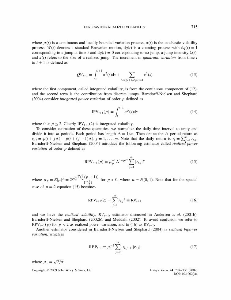
where ��t� is a continuous and locally bounded variation process, ��t� is the stochastic volatilityprocess, W�t� denotes a standard Brownian motion, dq(t) is a counting process with dq�t� D 1corresponding to a jump at time t and dq�t� D 0 corresponding to no jump, a jump intensity ��t�,and ��t� refers to the size of a realized jump. The increment in quadratic variation from time tto t C 1 is defined as

QVtC1 D∫ tC1

t�2�s�ds C

∑t<s�tC1,dq�s�D1

�2�s� �13�

where the first component, called integrated volatility, is from the continuous component of (12),and the second term is the contribution from discrete jumps. Barndorff-Nielsen and Shephard(2004) consider integrated power variation of order p defined as

IPVtC1�p� D∫ tC1

t�p�s�ds �14�

where 0 < p � 2. Clearly IPVtC1�2� is integrated volatility.To consider estimation of these quantities, we normalize the daily time interval to unity and

divide it into m periods. Each period has length D 1/m. Then define the period return asrt,j D p�t C j� � p�t C �j � 1��, j D 1, . . . , m. Note that the daily return is rt D ∑m

jD1 rt,j.Barndorff-Nielsen and Shephard (2004) introduce the following estimator called realized powervariation of order p defined as

RPVtC1�p� D ��1p 1�p/2

m∑jD1

jrt,jjp �15�

where �p D Ej�jp D 2p/2 � 12 �p C 1�� 1

2 �for p > 0, where � ¾ N�0, 1�. Note that for the special

case of p D 2 equation (15) becomes

RPVtC1�2� Dm∑

jD1

rt,j2 � RVtC1 �16�

and we have the realized volatility, RVtC1, estimator discussed in Andersen et al. (2001b),Barndorff-Nielsen and Shephard (2002b), and Meddahi (2002). To avoid confusion we refer toRPVtC1�p� for p < 2 as realized power variation, and to (16) as RVtC1.

Another estimator considered in Barndorff-Nielsen and Shephard (2004) is realized bipowervariation, which is

RBPtC1 � ��21

m∑jD2

jrt,j�1jjrt,jj �17�

where �1 D p2/�.



As shown by the papers discussed above, as m ! 1

RPVtC1�p�p!IPVtC1�p� D

∫ tC1

t�p�s�ds for p 2 �0, 2� �18�

RVtC1p!QVtC1 D

∫ tC1

t�2�s�ds C

∑�2�s� �19�

RBPtC1p!IPVtC1�2� D

∫ tC1

t�2�s�ds �20�

Note that the asymptotics operate within a fixed time interval by sampling more frequently.RV converges to quadratic variation, and the latter measures the ex post variation of the processregardless of the model or information set. Therefore, RV is the relevant quantity to focus on themodeling and forecasting of volatility. For further details on the relationship between RV and thesecond moments of returns see Andersen et al. (2003), Barndorff-Nielsen and Shephard (2002a,2005) and Meddahi (2003).

From these results, it follows that the jump component in QVtC1 can be estimated byRVtC1 � RBPtC1. RPVtC1�p� for p 2 �0, 2� and RBPtC1 are robust to jumps. Forsberg and Ghysels(2007), Ghysels et al. (2006) and Ghysels and Sinko (2006) have found that absolute returns (powervariation of order 1) improve volatility forecasting using criteria such as adjusted R2 and meansquared error. They argue that improvements are due to the higher predictability, less samplingerror and a robustness to jumps.

4. DATA

We investigate model forecasts for equity and exchange rate volatility over several forecasthorizons. For equity we consider the S&P 500 index by using the Spyder (Standard & Poor’sdepository receipts), which is an exchange traded fund that represents ownership in the S&P 500index. The ticker symbol is SPY. Since this asset is actively traded, it avoids the stale price effectof the S&P 500 index. The Spyder price transaction data are obtained from the Trade and Quotes(TAQ) database. After removing errors from the transaction data,8 a 5-minute grid from 9 : 30 to16 : 00 was constructed by finding the closest transaction price before or equal to each grid pointtime. The first observation of the day occurring just after 9 : 30 was used for the 9 : 30 grid time.From this grid, 5-minute intraday log returns are constructed. The intraday return data were usedto construct daily returns (open to close prices), and the associated realized volatility, realizedbipower variation and realized power variation of order 0.5, 1 and 1.5 following the previoussection. An adjusted estimator of RV and RBP to correct for market microstructure dynamicsis discussed below. Given the structural break found in early February 1997 in Liu and Maheu(2008) our data begin on 6 February 1997 and go to 30 March 2004.9 We reserve the first 35observations as startup values for the models. The final data have 1761 observations.

8 Data were collected with a TAQ correction indicator of 0 (regular trade) and when possible a 1 (trade later corrected).We also excluded any transaction with a sale condition of Z, which is a transaction reported on the tape out of timesequence, and with intervening trades between the trade time and the reported time on the tape. We also checked anyprice transaction change that was larger than 3%. A number of these were obvious errors and were removed.9 The main effect of the break is on the variance of log-volatility. We also investigated breaks in the JPY–USD andDEM–USD realized volatility data discussed below and found no evidence of parameter change.



High-frequency foreign exchange data on the JPY-USD and DEM-USD spot rates are fromOlsen Financial Technologies. We adopt the official conversion rate between DEM and euro after1 January 1999 to obtain the DEM–USD rate. Bid and ask quotes are recorded on a 5-minute gridwhen available. To fill in the missing values on the grid we take the closest previous bid and ask.The spot rate is taken as the logarithmic middle price for each grid point over a 24-hour day. Theend of a day is defined as 21 : 00:00 GMT and the start as 21 : 05:00 GMT. Weekends (21 : 05:00GMT Friday to 21 : 00:00 GMT Sunday) and slow trading dates (24–26, 31 December and 1–2January) and the moving holidays Good Friday, Easter Monday, Memorial Day, 4 July, Labor Day,Thanksgiving and the day after were removed. A few slow trading days were also removed. Fromthe remaining data, 5-minute returns where constructed, as well as the daily volatility measuresand the daily return (close to close prices). The sample period for FX data is from 3 February 1986to 30 December 2002. JPY–USD data has 4192 observations. The DEM–USD data have 4190observations. Conditioning on the first 35 observations leaves us 4157 observations (JPY–USD)and 4155 observations (DEM–USD).

4.1. Adjusting for Market Microstructure

It is generally accepted that there are dynamic dependencies in high-frequency returns inducedby market microstructure frictions (see Bandi and Russell, 2006; Hansen and Lunde, 2006a;Oomen, 2005; Zhang et al.; 2005) among others. The raw RV constructed from (16) can be aninconsistent estimator. To reduce the effect of market microstructure noise,10 we employ a kernel-based estimator suggested by Hansen and Lunde (2006a) which utilizes autocovariances of intradayreturns to construct realized volatility as

RVqt D

m∑iD1

r2t,i C 2

q∑wD1

(1 � w

q C 1

) m�w∑iD1

rt,irt,iCw �21�

where rt,i is the ith logarithmic return during day t, and q is a small non-negative integer.The theoretical results concerning this estimator is due to Barndorff-Nielsen et al. (2006a). ThisBartlett-type weight ensures a positive estimate, and Barndorff-Nielsen et al. (2006b) show that itis almost identical to the subsample-based estimator of Zhang et al. (2005).

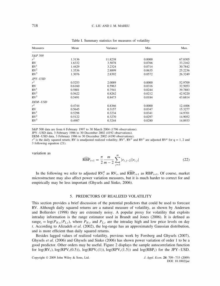
We list the summary statistics for daily squared returns, unadjusted RV and the adjusted RVfor q D 1, 2 and 3 in Table I. As a benchmark, the average daily squared return can be treatedas an unbiased estimator of the mean of latent volatility. However, it is very noisy, which can beseen from its large variance. The RV row lists the statistics for the unadjusted RV. The averagedifference between the mean of daily squared returns and unadjusted RV is fairly large. Thissuggests significant market microstructure biases. The adjusted RV provides an improvement. Inour work we use q D 3. The time series of adjusted log�RVt� measures are shown in Figure 1.

Market microstructure also contaminates bipower variation. As in Andersen et al. (2007) andHuang and Tauchen (2005), using staggered returns will decrease the correlation in adjacent returnsinduced by the microstructure noise. Following their suggestion, we use an adjusted bipower

10 An alternative is to sample the price process at a lower frequency to minimize market microstructure contamination.However, the asymptotics in Section 3 suggest a loss of information in lower sampling frequencies.



Table I. Summary statistics for measures of volatility

Measures Mean Variance Min. Max.

S&P 500r2 1.3136 11.8238 0.0000 67.8305RV 1.6332 3.5078 0.0766 33.2162RV1 1.4429 3.2324 0.0714 30.7842RV2 1.3536 2.8899 0.0635 25.2236RV3 1.3076 2.8392 0.0572 26.3249

JPY–USDr2 0.5253 2.0089 0.0000 52.9709RV 0.6160 0.5963 0.0316 32.5053RV1 0.5801 0.7541 0.0244 39.7883RV2 0.5622 0.8262 0.0212 42.9220RV3 0.5491 0.8473 0.0184 43.6814

DEM–USDr2 0.4744 0.8366 0.0000 12.4406RV 0.5645 0.3157 0.0347 15.3277RV1 0.5298 0.3234 0.0341 14.9701RV2 0.5122 0.3270 0.0297 14.9052RV3 0.4987 0.3244 0.0280 14.8933

S&P 500 data are from 6 February 1997 to 30 March 2004 (1796 observations).JPY–USD data, 3 February 1986 to 30 December 2002 (4192 observations).DEM–USD data, 3 February 1986 to 30 December 2002 (4190 observations).r2 is the daily squared return; RV is unadjusted realized volatility; RV1, RV2 and RV3 are adjusted RVq for q D 1, 2 and3 following equation (21).

variation as

RBPtC1 D �

2

m

m � 2

m∑jD3

jrt,j�2jjrt,jj �22�

In the following we refer to adjusted RVqt as RVt, and RBPtC1 as RBPtC1. Of course, market

microstructure may also affect power variation measures, but it is much harder to correct for andempirically may be less important (Ghysels and Sinko, 2006).

5. PREDICTORS OF REALIZED VOLATILITY

This section provides a brief discussion of the potential predictors that could be used to forecastRV. Although daily squared returns are a natural measure of volatility, as shown by Andersenand Bollerslev (1998) they are extremely noisy. A popular proxy for volatility that exploitsintraday information is the range estimator used in Brandt and Jones (2006). It is defined asranget D log�PH,t/PL,t�, where PH,t and PL,t are the intraday high and low price levels on dayt. According to Alizadeh et al. (2002), the log-range has an approximately Gaussian distribution,and is more efficient than daily squared returns.

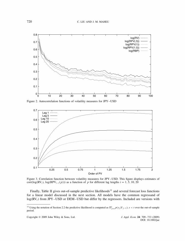
Besides lagged values of realized volatility, previous work by Forsberg and Ghysels (2007),Ghysels et al. (2006) and Ghysels and Sinko (2006) has shown power variation of order 1 to be agood predictor. Other orders may be useful. Figure 2 displays the sample autocorrelation functionfor log�RVt�, log�RPVt�0.5��, log�RPVt�1��, log�RPVt�1.5�� and log�RBPt� for the JPY–USD.



-3

-2

-1

0

1

2

3

4

2004200220001998

S&P 500

-4

-3

-2

-1

0

1

2

3

4

2000199619921988

JPY/USD

-4

-3

-2

-1

0

1

2

3

2000199619921988

DEM/USD

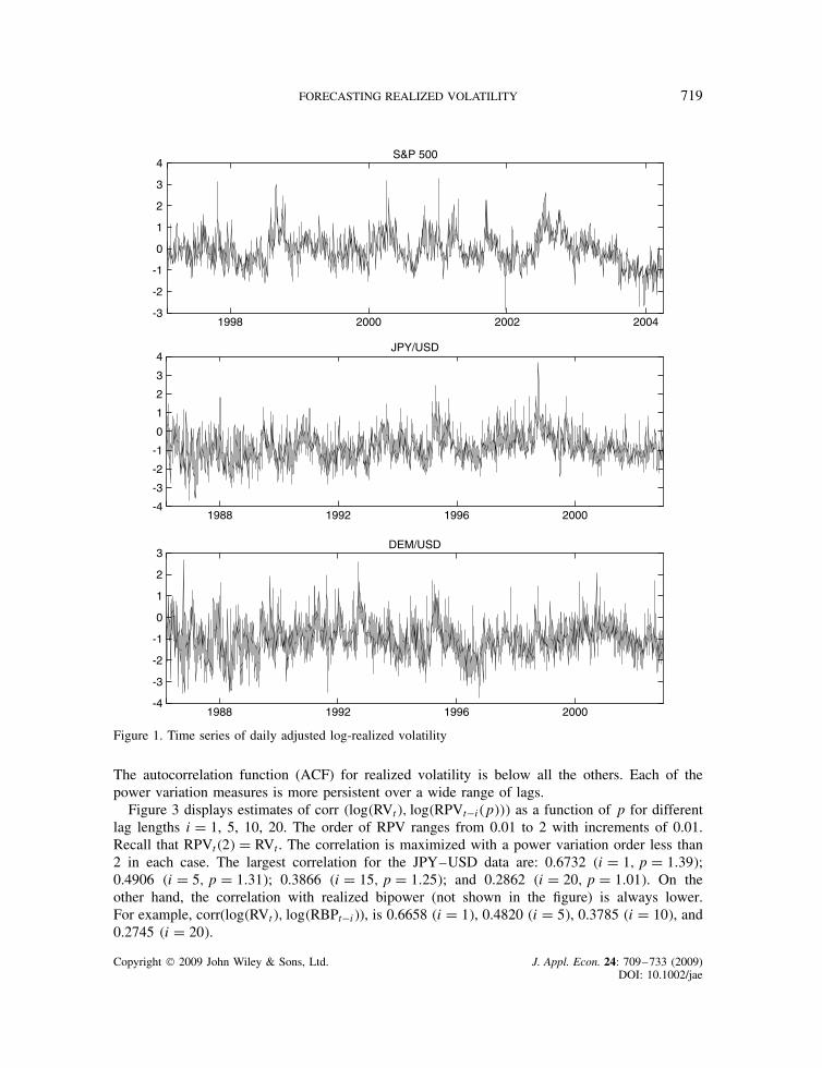
Figure 1. Time series of daily adjusted log-realized volatility

The autocorrelation function (ACF) for realized volatility is below all the others. Each of thepower variation measures is more persistent over a wide range of lags.

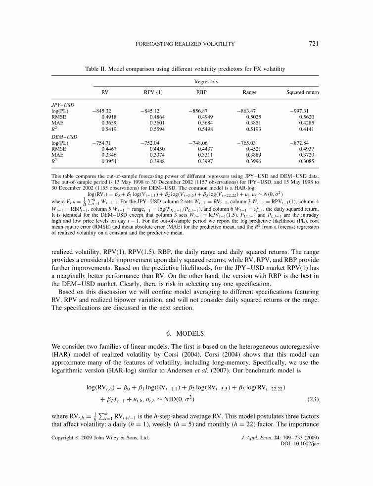
Figure 3 displays estimates of corr �log�RVt�, log�RPVt�i�p�� as a function of p for differentlag lengths i D 1, 5, 10, 20. The order of RPV ranges from 0.01 to 2 with increments of 0.01.Recall that RPVt�2� D RVt. The correlation is maximized with a power variation order less than2 in each case. The largest correlation for the JPY–USD data are: 0.6732 �i D 1, p D 1.39�;0.4906 �i D 5, p D 1.31�; 0.3866 �i D 15, p D 1.25�; and 0.2862 �i D 20, p D 1.01�. On theother hand, the correlation with realized bipower (not shown in the figure) is always lower.For example, corr(log�RVt�, log�RBPt�i�), is 0.6658 �i D 1�, 0.4820 �i D 5�, 0.3785 �i D 10�, and0.2745 �i D 20�.



0

0.1

0.2

0.3

0.4

0.5

0.6

0.7

0.8

1009080706050403020100

log(RV)log(RPV(.5))log(RPV(1))

log(RPV(1.5))log(RBP)

Figure 2. Autocorrelation functions of volatility measures for JPY–USD

0.1

0.2

0.3

0.4

0.5

0.6

0.7

21.751.51.2510.750.50.25

Order of PV

Lag 1Lag 5

Lag 10Lag 20

Figure 3. Correlation function between volatility measures for JPY–USD. This figure displays estimates ofcorr(log�RVt�, log�RPVt�i�p��) as a function of p for different lag lengths i D 1, 5, 10, 20

Finally, Table II gives out-of-sample predictive likelihoods11 and several forecast loss functionsfor a linear model discussed in the next section. All models have the common regressand oflog�RVt� from JPY–USD or DEM–USD but differ by the regressors. Included are versions with

11 Using the notation of Section 2.2 the predictive likelihood is computed as tjDsp�yjjYj�1�, s < t over the out-of-sample

period.



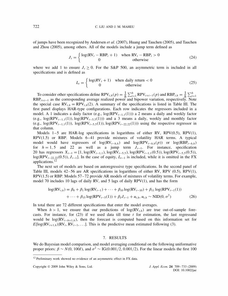
Table II. Model comparison using different volatility predictors for FX volatility

Regressors

RV RPV (1) RBP Range Squared return

JPY–USDlog(PL) �845.32 �845.12 �856.87 �863.47 �997.31RMSE 0.4918 0.4864 0.4949 0.5025 0.5620MAE 0.3659 0.3601 0.3684 0.3851 0.4285R2 0.5419 0.5594 0.5498 0.5193 0.4141

DEM–USDlog(PL) �754.71 �752.04 �748.06 �765.03 �872.84RMSE 0.4467 0.4450 0.4437 0.4521 0.4937MAE 0.3346 0.3374 0.3311 0.3889 0.3729R2 0.3954 0.3988 0.3997 0.3996 0.3085

This table compares the out-of-sample forecasting power of different regressors using JPY–USD and DEM–USD data.The out-of-sample period is 13 May 1998 to 30 December 2002 (1157 observations) for JPY–USD, and 15 May 1998 to30 December 2002 (1155 observations) for DEM–USD. The common model is a HAR-log:

log�RVt� D ˇ0 C ˇ1 log�Vt�1,1� C ˇ2 log�Vt�5,5� C ˇ3 log�Vt�22,22� C ut, ut ¾ N�0, �2�where Vt,h D 1

h∑h

iD1 WtCi�1. For the JPY–USD column 2 sets Wt�1 D RVt�1, column 3 Wt�1 D RPVt�1�1�, column 4Wt�1 D RBPt�1, column 5 Wt�1 D ranget�1 D log�PH,t�1/PL,t�1�, and column 6 Wt�1 D r2

t�1, the daily squared return.It is identical for the DEM–USD except that column 3 sets Wt�1 D RPVt�1�1.5�. PH,t�1 and PL,t�1 are the intradayhigh and low price levels on day t � 1. For the out-of-sample period we report the log predictive likelihood (PL), rootmean square error (RMSE) and mean absolute error (MAE) for the predictive mean, and the R2 from a forecast regressionof realized volatility on a constant and the predictive mean.

realized volatility, RPV(1), RPV(1.5), RBP, the daily range and daily squared returns. The rangeprovides a considerable improvement upon daily squared returns, while RV, RPV, and RBP providefurther improvements. Based on the predictive likelihoods, for the JPY–USD market RPV(1) hasa marginally better performance than RV. On the other hand, the version with RBP is the best inthe DEM–USD market. Clearly, there is risk in selecting any one specification.

Based on this discussion we will confine model averaging to different specifications featuringRV, RPV and realized bipower variation, and will not consider daily squared returns or the range.The specifications are discussed in the next section.

6. MODELS

We consider two families of linear models. The first is based on the heterogeneous autoregressive(HAR) model of realized volatility by Corsi (2004). Corsi (2004) shows that this model canapproximate many of the features of volatility, including long-memory. Specifically, we use thelogarithmic version (HAR-log) similar to Andersen et al. (2007). Our benchmark model is

log�RVt,h� D ˇ0 C ˇ1 log�RVt�1,1� C ˇ2 log�RVt�5,5� C ˇ3 log�RVt�22,22�

C ˇJJt�1 C ut,h, ut,h ¾ NID�0, �2� �23�

where RVt,h D 1h

∑hiD1 RVtCi�1 is the h-step-ahead average RV. This model postulates three factors

that affect volatility: a daily �h D 1�, weekly �h D 5� and monthly �h D 22� factor. The importance



of jumps have been recognized by Andersen et al. (2007), Huang and Tauchen (2005), and Tauchenand Zhou (2005), among others. All of the models include a jump term defined as

Jt D{

log�RVt � RBPt C 1� when RVt � RBPt > 00 otherwise

�24�

where we add 1 to ensure Jt ½ 0. For the S&P 500, an asymmetric term is included in allspecifications and is defined as

Lt D{

log�RVt C 1� when daily return < 00 otherwise

�25�

To consider other specifications define RPVt,h�p� D 1h

∑hiD1 RPVtCi�1�p� and RBPt,h D 1

h∑h

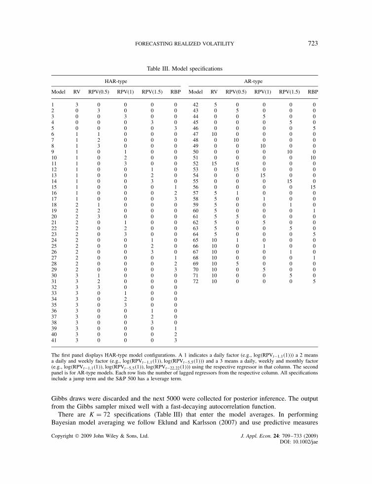
iD1RBPtCi�1 as the corresponding average realized power and bipower variation, respectively. Notethe special case RVt,h D RPVt,h�2�. A summary of the specifications is listed in Table III. Thefirst panel displays HAR-type configurations. Each row indicates the regressors included in amodel. A 1 indicates a daily factor (e.g., log�RPVt�1,1�1��) a 2 means a daily and weekly factor(e.g., log�RPVt�1,1�1��, log�RPVt�5,5�1��) and a 3 means a daily, weekly and monthly factor(e.g., log�RPVt�1,1�1��, log�RPVt�5,5�1��, log�RPVt�22,22�1��) using the respective regressor inthat column.

Models 1–5 are HAR-log specifications in logarithms of either RV, RPV(0.5), RPV(1),RPV(1.5) or RBP. Models 6–41 provide mixtures of volatility HAR terms. A typicalmodel would have regressors of log�RVt�h,h� and log�RPVt�h,h�p�� or log�RBPt�h,h�for h D 1, 5 and 22 as well as a jump term Jt�1. For instance, specification20 has regressors Xt�1 D [1, log�RVt�1,1�, log�RVt�5,5�, log�RPVt�1,1�0.5��, log�RPVt�5,5�0.5��,log�RPVt�22,22�0.5��, Jt�1]. In the case of equity, Lt�1 is included, while it is omitted in the FXapplications.12

The next set of models are based on autoregressive type specifications. In the second panel ofTable III, models 42–56 are AR specifications in logarithms of either RV, RPV (0.5), RPV(1),RPV(1.5) or RBP. Models 57–72 provide AR models of mixtures of volatility terms. For example,model 70 includes 10 lags of daily RV, and 5 lags of daily RPV(1), and has the form

log�RVt,h� D ˇ0 C ˇ1 log�RVt�1� C Ð Ð Ð C ˇ10 log�RVt�10� C ˇ11 log�RPVt�1�1��

C Ð Ð Ð C ˇ15 log�RPVt�5�1�� C ˇJJt�1 C ut,h, ut,h ¾ NID�0, �2� �26�

In total there are 72 different specifications that enter the model averages.When h > 1, we ensure that our predictions of log�RVt,h� are true out-of-sample fore-

casts. For instance, for (23) if we used data till time t for estimation, the last regressandwould be log�RVt�hC1,h�, then the forecast is computed based on this information set forE[log�RVtC1,h�jRVt, RVt�1, . . .]. This is the predictive mean estimated following (3).

7. RESULTS

We do Bayesian model comparison, and model averaging conditional on the following uniformativeproper priors: ˇ ¾ N�0, 100I�, and �2 ¾ IG�0.001/2, 0.001/2�. For the linear models the first 100

12 Preliminary work showed no evidence of an asymmetric effect in FX data.



Table III. Model specifications

HAR-type AR-type

Model RV RPV(0.5) RPV(1) RPV(1.5) RBP Model RV RPV(0.5) RPV(1) RPV(1.5) RBP

1 3 0 0 0 0 42 5 0 0 0 02 0 3 0 0 0 43 0 5 0 0 03 0 0 3 0 0 44 0 0 5 0 04 0 0 0 3 0 45 0 0 0 5 05 0 0 0 0 3 46 0 0 0 0 56 1 1 0 0 0 47 10 0 0 0 07 1 2 0 0 0 48 0 10 0 0 08 1 3 0 0 0 49 0 0 10 0 09 1 0 1 0 0 50 0 0 0 10 010 1 0 2 0 0 51 0 0 0 0 1011 1 0 3 0 0 52 15 0 0 0 012 1 0 0 1 0 53 0 15 0 0 013 1 0 0 2 0 54 0 0 15 0 014 1 0 0 3 0 55 0 0 0 15 015 1 0 0 0 1 56 0 0 0 0 1516 1 0 0 0 2 57 5 1 0 0 017 1 0 0 0 3 58 5 0 1 0 018 2 1 0 0 0 59 5 0 0 1 019 2 2 0 0 0 60 5 0 0 0 120 2 3 0 0 0 61 5 5 0 0 021 2 0 1 0 0 62 5 0 5 0 022 2 0 2 0 0 63 5 0 0 5 023 2 0 3 0 0 64 5 0 0 0 524 2 0 0 1 0 65 10 1 0 0 025 2 0 0 2 0 66 10 0 1 0 026 2 0 0 3 0 67 10 0 0 1 027 2 0 0 0 1 68 10 0 0 0 128 2 0 0 0 2 69 10 5 0 0 029 2 0 0 0 3 70 10 0 5 0 030 3 1 0 0 0 71 10 0 0 5 031 3 2 0 0 0 72 10 0 0 0 532 3 3 0 0 033 3 0 1 0 034 3 0 2 0 035 3 0 3 0 036 3 0 0 1 037 3 0 0 2 038 3 0 0 3 039 3 0 0 0 140 3 0 0 0 241 3 0 0 0 3

The first panel displays HAR-type model configurations. A 1 indicates a daily factor (e.g., log�RPVt�1,1�1��) a 2 meansa daily and weekly factor (e.g., log�RPVt�1,1�1��, log�RPVt�5,5�1��) and a 3 means a daily, weekly and monthly factor(e.g., log�RPVt�1,1�1��, log�RPVt�5,5�1��, log�RPVt�22,22�1��) using the respective regressor in that column. The secondpanel is for AR-type models. Each row lists the number of lagged regressors from the respective column. All specificationsinclude a jump term and the S&P 500 has a leverage term.

Gibbs draws were discarded and the next 5000 were collected for posterior inference. The outputfrom the Gibbs sampler mixed well with a fast-decaying autocorrelation function.

There are K D 72 specifications (Table III) that enter the model averages. In performingBayesian model averaging we follow Eklund and Karlsson (2007) and use predictive measures



to combine individual models. We set the model probabilities to P�Mk� D 1/K, k D 1, . . . , K atobservation 500.13 Thereafter we update model probabilities according to Bayes’ rule. The trainingsample of 500 observations only affects BMA, and Section 7.3 shows the results are robust todifferent sample sizes. The effect of the training sample is to put more weight on recent modelperformance. As Eklund and Karlsson (2007) show, this provides protection against in-sampleoverfitting and can improve forecast performance. To compute the predictive likelihood from theend of the training sample to the last in-sample observation we use the Chib (1995) method14 (seethe Appendix for details); thereafter we update model probabilities period by period using (7) and(9).

The in-sample observations are 1000 for S&P 500, and 3000 for both JPY-USD and DEM-USD.The out-of-sample period extends from 16 March 2001 to 30 March 2004 (761 observations) forS&P 500, 13 May 1998 to 30 December 2002 (1157 observations) for JPY–USD, and 15 May1998 to 30 December 2002 (1155 observations) for DEM–USD.

7.1. Bayesian Model Averaging

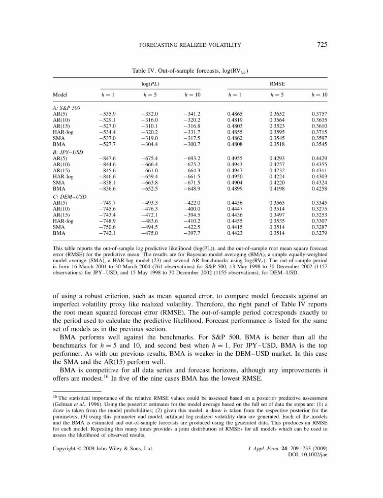
The predictive likelihood for BMA along with several benchmark alternatives is displayed in theleft panel of Table IV.15 Included are autoregressive models in log�RVt�, the HAR-log specificationin (23), and a simple model average (SMA) which assumes equal weighting across all modelsthrough time.

Beginning with the S&P 500, BMA is very competitive. When h D 1, the log predictivelikelihood is larger than all the benchmarks except for the AR(15) model, where BMA and AR(15)have very close values. The evidence for h D 5 and h D 10 is stronger. The log(PL) for the BMAis about 6 and 16 points larger than those from the best benchmarks. We also find the SMA isdominated by many of the benchmarks, and it has poor performance compared with BMA. Thedifference between these model averages is that BMA weights models based on predictive contentwhile the SMA ignores it.

For JPY–USD market the Bayesian model average outperforms all the benchmarks for eachtime horizon. Compared to the HAR-log model used in Andersen et al. (2007) the log predictiveBayes factor in favor of BMA is 10.0, 6.9, and 12.6 for h D 1, 5, and 10, respectively. It alsoperforms well for DEM–USD when h D 1. However, for h D 5 and h D 10 the BMA is secondto the AR(15) model.

In summary, in six out of nine cases BMA delivers the best performance in terms of densityforecasts, and when it is not the top model it is a close second.

7.2. Out-of-Sample Point Forecasts

Although we focus on the predictive likelihood to measure predictive content, it is interesting toconsider the out-of-sample point forecasts of average log volatility based on the predictive mean.Recent work by Hansen and Lunde (2006b) and Patton (2006) has emphasized the importance

13 For example, using (9) we set P�Mk jY500� � 1/K for k D 1, . . . , K and build up the model probabilities as new dataarrive.14 For instance, using the notation in Section 2, the log predictive likelihood for y501, . . . , yT, where yT is the last in-sampleobservation, can be decomposed as log�p�YT�� log�p�Y500�� and each term estimated by Chib (1995).15 The full set of results for individual models is available upon request from the authors.



Table IV. Out-of-sample forecasts, log�RVt,h�

log�PL� RMSE

Model h D 1 h D 5 h D 10 h D 1 h D 5 h D 10

A: S&P 500AR(5) �535.9 �332.0 �341.2 0.4865 0.3652 0.3757AR(10) �529.1 �316.0 �320.2 0.4819 0.3564 0.3635AR(15) �527.0 �310.1 �316.8 0.4803 0.3523 0.3610HAR-log �534.4 �320.2 �331.7 0.4855 0.3595 0.3715SMA �537.0 �319.0 �317.5 0.4862 0.3545 0.3597BMA �527.7 �304.4 �300.7 0.4808 0.3518 0.3545

B: JPY–USDAR(5) �847.6 �675.4 �693.2 0.4955 0.4293 0.4429AR(10) �844.6 �666.4 �675.2 0.4943 0.4257 0.4355AR(15) �845.6 �661.0 �664.3 0.4947 0.4232 0.4311HAR-log �846.6 �659.4 �661.5 0.4950 0.4224 0.4303SMA �838.1 �663.8 �671.5 0.4904 0.4220 0.4324BMA �836.6 �652.5 �648.9 0.4899 0.4198 0.4258

C: DEM–USDAR(5) �749.7 �493.3 �422.0 0.4456 0.3565 0.3345AR(10) �745.6 �476.3 �400.0 0.4447 0.3514 0.3275AR(15) �743.4 �472.1 �394.5 0.4436 0.3497 0.3253HAR-log �748.9 �483.6 �410.2 0.4455 0.3535 0.3307SMA �750.6 �494.5 �422.5 0.4415 0.3514 0.3287BMA �742.1 �475.0 �397.7 0.4423 0.3514 0.3279

This table reports the out-of-sample log predictive likelihood (log(PL)), and the out-of-sample root mean square forecasterror (RMSE) for the predictive mean. The results are for Bayesian model averaging (BMA), a simple equally-weightedmodel average (SMA), a HAR-log model (23) and several AR benchmarks using log�RVt�. The out-of-sample periodis from 16 March 2001 to 30 March 2004 (761 observations) for S&P 500, 13 May 1998 to 30 December 2002 (1157observations) for JPY–USD, and 15 May 1998 to 30 December 2002 (1155 observations), for DEM–USD.

of using a robust criterion, such as mean squared error, to compare model forecasts against animperfect volatility proxy like realized volatility. Therefore, the right panel of Table IV reportsthe root mean squared forecast error (RMSE). The out-of-sample period corresponds exactly tothe period used to calculate the predictive likelihood. Forecast performance is listed for the sameset of models as in the previous section.

BMA performs well against the benchmarks. For S&P 500, BMA is better than all thebenchmarks for h D 5 and 10, and second best when h D 1. For JPY–USD, BMA is the topperformer. As with our previous results, BMA is weaker in the DEM–USD market. In this casethe SMA and the AR(15) perform well.

BMA is competitive for all data series and forecast horizons, although any improvements itoffers are modest.16 In five of the nine cases BMA has the lowest RMSE.

16 The statistical importance of the relative RMSE values could be assessed based on a posterior predictive assessment(Gelman et al., 1996). Using the posterior estimates for the model average based on the full set of data the steps are: (1) adraw is taken from the model probabilities; (2) given this model, a draw is taken from the respective posterior for theparameters; (3) using this parameter and model, artificial log-realized volatility data are generated. Each of the modelsand the BMA is estimated and out-of-sample forecasts are produced using the generated data. This produces an RMSEfor each model. Repeating this many times provides a joint distribution of RMSEs for all models which can be used toassess the likelihood of observed results.



7.3. Training Sample

The above results are based on model combination using predictive measures. As previouslymentioned, we set the model probabilities to P�Mk� D 1/K, k D 1, . . . , K at observation 500;thereafter model probabilities are updated according to Bayes rule. This training sample of 500observations puts more weight on recent model performance and less on past model performance.To investigate the robustness of BMA to the size of the training sample, we calculate the resultswith different sample sizes as well as no training sample. Results are summarized in Table V forDEM–USD with similar results for the other data. Focusing on the predictive likelihood, we seethat using more recent predictive measures has some benefit for h D 10.

7.4. The Role of Power Variation

In this section we investigate why BMA performs well. One reason is that it weights individualmodels based on past predictive content through the model probabilities. Over time modelperformance changes and BMA responds to it. Another possibility is that the specifications withpower variation are better than existing models that only use RV.

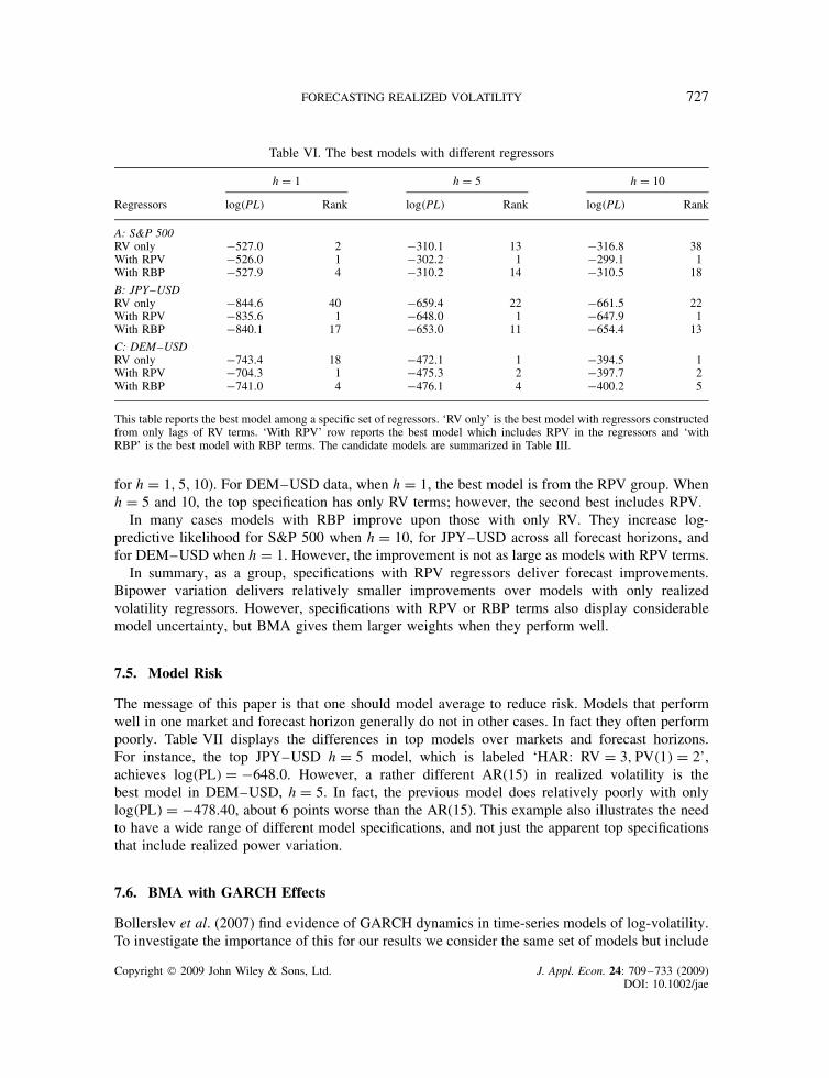
To focus on this latter question we divide all the models that enter BMA into three groupsaccording to their regressors. These are: the ‘RV only group’, which includes all models that haveregressors constructed from only lag terms of log�RVt�; the ‘RPV group’ includes all modelsin which at least one RPV regressor is used; and the ‘RBP group’ is all models that have RBPregressors. Table VI reports the predictive likelihood of the best models within each group for eachof the forecast horizons h D 1, 5, and 10. The rank of the model among the K D 72 alternativesis also displayed.

Including RPV terms can improve forecasting power. For S&P 500 when h D 1, if we excludeRPV regressors, the best individual model has a log-predictive likelihood �527.0 with a rank of2 out of the full 72 models. Among the models with RPV, the best one has log(PL) of �526.0and it is also the best model overall. For h D 5, including RPV increases log(PL) from �310.1 forthe RV group to �302.2 (rank from 13 to 1). For h D 10, the best RPV model achieves a �299.1with rank 1, while the best RV model is �316.8 with rank 38.

The results from the JPY–USD market provide very similar supportive evidence for the inclusionof RPV. In panel B, the best models in the RPV group dominate those in the RV only group acrossh with much higher predictive likelihood values (�835.6 vs. �844.6 for h D 1, �648.0 vs. �659.4for h D 5 and �647.9 vs. �661.5 for h D 10) and ranking (1, 1, 1 compared with 40, 22 and 22

Table V. Robustness to training sample size, DEM–USD

h D 1 h D 5 h D 10

Obs. log(PL) RMSE log(PL) RMSE log(PL) RMSE

0 �743.1 0.4426 �476.9 0.3514 �407.5 0.3308200 �741.5 0.4419 �475.3 0.3515 �397.7 0.3279500 �742.1 0.4423 �475.0 0.3514 �397.7 0.32791000 �742.4 0.4424 �474.3 0.3511 �397.4 0.3282

The first column is the number of observations in the training sample. A 0 denotes no training sample. Other columnsshow the results for BMA, including log predictive likelihood (PL) and root mean squared forecast error (RMSE).



Table VI. The best models with different regressors

h D 1 h D 5 h D 10

Regressors log�PL� Rank log�PL� Rank log�PL� Rank

A: S&P 500RV only �527.0 2 �310.1 13 �316.8 38With RPV �526.0 1 �302.2 1 �299.1 1With RBP �527.9 4 �310.2 14 �310.5 18

B: JPY–USDRV only �844.6 40 �659.4 22 �661.5 22With RPV �835.6 1 �648.0 1 �647.9 1With RBP �840.1 17 �653.0 11 �654.4 13

C: DEM–USDRV only �743.4 18 �472.1 1 �394.5 1With RPV �704.3 1 �475.3 2 �397.7 2With RBP �741.0 4 �476.1 4 �400.2 5

This table reports the best model among a specific set of regressors. ‘RV only’ is the best model with regressors constructedfrom only lags of RV terms. ‘With RPV’ row reports the best model which includes RPV in the regressors and ‘withRBP’ is the best model with RBP terms. The candidate models are summarized in Table III.

for h D 1, 5, 10). For DEM–USD data, when h D 1, the best model is from the RPV group. Whenh D 5 and 10, the top specification has only RV terms; however, the second best includes RPV.

In many cases models with RBP improve upon those with only RV. They increase log-predictive likelihood for S&P 500 when h D 10, for JPY–USD across all forecast horizons, andfor DEM–USD when h D 1. However, the improvement is not as large as models with RPV terms.

In summary, as a group, specifications with RPV regressors deliver forecast improvements.Bipower variation delivers relatively smaller improvements over models with only realizedvolatility regressors. However, specifications with RPV or RBP terms also display considerablemodel uncertainty, but BMA gives them larger weights when they perform well.

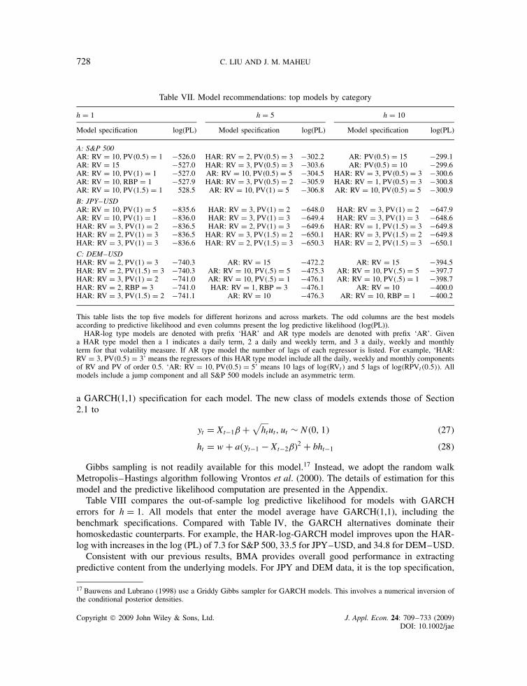
7.5. Model Risk

The message of this paper is that one should model average to reduce risk. Models that performwell in one market and forecast horizon generally do not in other cases. In fact they often performpoorly. Table VII displays the differences in top models over markets and forecast horizons.For instance, the top JPY–USD h D 5 model, which is labeled ‘HAR: RV D 3, PV�1� D 2’,achieves log�PL� D �648.0. However, a rather different AR(15) in realized volatility is thebest model in DEM–USD, h D 5. In fact, the previous model does relatively poorly with onlylog�PL� D �478.40, about 6 points worse than the AR(15). This example also illustrates the needto have a wide range of different model specifications, and not just the apparent top specificationsthat include realized power variation.

7.6. BMA with GARCH Effects

Bollerslev et al. (2007) find evidence of GARCH dynamics in time-series models of log-volatility.To investigate the importance of this for our results we consider the same set of models but include



Table VII. Model recommendations: top models by category

h D 1 h D 5 h D 10

Model specification log(PL) Model specification log(PL) Model specification log(PL)

A: S&P 500AR: RV D 10, PV�0.5� D 1 �526.0 HAR: RV D 2, PV�0.5� D 3 �302.2 AR: PV�0.5� D 15 �299.1AR: RV D 15 �527.0 HAR: RV D 3, PV�0.5� D 3 �303.6 AR: PV�0.5� D 10 �299.6AR: RV D 10, PV�1� D 1 �527.0 AR: RV D 10, PV�0.5� D 5 �304.5 HAR: RV D 3, PV�0.5� D 3 �300.6AR: RV D 10, RBP D 1 �527.9 HAR: RV D 3, PV�0.5� D 2 �305.9 HAR: RV D 1, PV�0.5� D 3 �300.8AR: RV D 10, PV�1.5� D 1 528.5 AR: RV D 10, PV�1� D 5 �306.8 AR: RV D 10, PV�0.5� D 5 �300.9

B: JPY–USDAR: RV D 10, PV�1� D 5 �835.6 HAR: RV D 3, PV�1� D 2 �648.0 HAR: RV D 3, PV�1� D 2 �647.9AR: RV D 10, PV�1� D 1 �836.0 HAR: RV D 3, PV�1� D 3 �649.4 HAR: RV D 3, PV�1� D 3 �648.6HAR: RV D 3, PV�1� D 2 �836.5 HAR: RV D 2, PV�1� D 3 �649.6 HAR: RV D 1, PV�1.5� D 3 �649.8HAR: RV D 2, PV�1� D 3 �836.5 HAR: RV D 3, PV�1.5� D 2 �650.1 HAR: RV D 3, PV�1.5� D 2 �649.8HAR: RV D 3, PV�1� D 3 �836.6 HAR: RV D 2, PV�1.5� D 3 �650.3 HAR: RV D 2, PV�1.5� D 3 �650.1

C: DEM–USDHAR: RV D 2, PV�1� D 3 �740.3 AR: RV D 15 �472.2 AR: RV D 15 �394.5HAR: RV D 2, PV�1.5� D 3 �740.3 AR: RV D 10, PV�.5� D 5 �475.3 AR: RV D 10, PV�.5� D 5 �397.7HAR: RV D 3, PV�1� D 2 �741.0 AR: RV D 10, PV�.5� D 1 �476.1 AR: RV D 10, PV�.5� D 1 �398.7HAR: RV D 2, RBP D 3 �741.0 HAR: RV D 1, RBP D 3 �476.1 AR: RV D 10 �400.0HAR: RV D 3, PV�1.5� D 2 �741.1 AR: RV D 10 �476.3 AR: RV D 10, RBP D 1 �400.2

This table lists the top five models for different horizons and across markets. The odd columns are the best modelsaccording to predictive likelihood and even columns present the log predictive likelihood (log(PL)).

HAR-log type models are denoted with prefix ‘HAR’ and AR type models are denoted with prefix ‘AR’. Givena HAR type model then a 1 indicates a daily term, 2 a daily and weekly term, and 3 a daily, weekly and monthlyterm for that volatility measure. If AR type model the number of lags of each regressor is listed. For example, ‘HAR:RV D 3, PV�0.5� D 3’ means the regressors of this HAR type model include all the daily, weekly and monthly componentsof RV and PV of order 0.5. ‘AR: RV D 10, PV�0.5� D 5’ means 10 lags of log�RVt� and 5 lags of log�RPVt�0.5��. Allmodels include a jump component and all S&P 500 models include an asymmetric term.

a GARCH(1,1) specification for each model. The new class of models extends those of Section2.1 to

yt D Xt�1ˇ C√

htut, ut ¾ N�0, 1� �27�

ht D w C a�yt�1 � Xt�2ˇ�2 C bht�1 �28�

Gibbs sampling is not readily available for this model.17 Instead, we adopt the random walkMetropolis–Hastings algorithm following Vrontos et al. (2000). The details of estimation for thismodel and the predictive likelihood computation are presented in the Appendix.

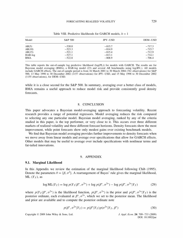
Table VIII compares the out-of-sample log predictive likelihood for models with GARCHerrors for h D 1. All models that enter the model average have GARCH(1,1), including thebenchmark specifications. Compared with Table IV, the GARCH alternatives dominate theirhomoskedastic counterparts. For example, the HAR-log-GARCH model improves upon the HAR-log with increases in the log (PL) of 7.3 for S&P 500, 33.5 for JPY–USD, and 34.8 for DEM–USD.

Consistent with our previous results, BMA provides overall good performance in extractingpredictive content from the underlying models. For JPY and DEM data, it is the top specification,

17 Bauwens and Lubrano (1998) use a Griddy Gibbs sampler for GARCH models. This involves a numerical inversion ofthe conditional posterior densities.



Table VIII. Predictive likelihoods for GARCH models, h D 1

Model S&P 500 JPY–USD DEM–USD

AR(5) �530.0 �815.7 �717.3AR(10) �523.3 �814.9 �715.7AR(15) �521.1 �815.4 �712.9HAR-log �527.1 �813.1 �714.1BMA �522.8 �808.9 �706.4

This table reports the out-of-sample log predictive likelihood (log(PL)) for models with GARCH. The results are forBayesian model averaging (BMA), a HAR-log model (23) and several AR benchmarks using log�RVt�. All modelsinclude GARCH effects. The out-of-sample period is from 16 March 2001 to 30 March 2004 (761 observations) for S&P500, 13 May 1998 to 30 December 2002 (1157 observations) for JPY–USD, and 15 May 1998 to 30 December 2002(1155 observations), for DEM–USD.

while it is a close second for the S&P 500. In summary, averaging over a better class of models,BMA remains a useful approach to reduce model risk and provide consistently good densityforecasts.

8. CONCLUSION

This paper advocates a Bayesian model-averaging approach to forecasting volatility. Recentresearch provides a range of potential regressors. Model averaging reduces the risk comparedto selecting any one particular model. Bayesian model averaging, ranked by any of the criteriastudied in this paper, is the top performer, or very close to it. This occurs over three differentmarkets of realized volatility and three different forecast horizons. Density forecasts show the mostimprovement, while point forecasts show only modest gains over existing benchmark models.

We find that Bayesian model averaging provides further improvements to density forecasts whenwe move away from linear models and average over specifications that allow for GARCH effects.Other models that may be useful to average over include specifications with nonlinear terms andfat-tailed innovations.

9. APPENDIX

9.1. Marginal Likelihood

In this Appendix we review the estimation of the marginal likelihood following Chib (1995).Denote the parameters � D fˇ, �2g. A rearrangement of Bayes’ rule gives the marginal likelihood,ML �YT�, as

log ML�YT� D log p�YTjˇŁ, �2Ł� C log p�ˇŁ, �2Ł� � log p�ˇŁ, �2ŁjYT� �29�

where p�YTjˇŁ, �2Ł� is the likelihood function, p�ˇŁ, �2Ł� is the prior and p�ˇŁ, �2ŁjYT� is theposterior ordinate, each evaluated at ˇŁ, �2Ł, which we set to the posterior mean. The likelihoodand prior are available and to compute the posterior ordinate note

p�ˇŁ, �2ŁjYT� D p�ˇŁjYT�p��2ŁjYT, ˇŁ� �30�



The first term at the right-hand side is

p�ˇŁjYT� D∫

p�ˇŁjYT, �2�p��2jYT�d�2 �31�

and can be estimated as p� ˇŁjYT� D 1N

N∑iD1

p�ˇŁjYT, �2�i��, where the draws f�2�i�gNiD1 are available

directly from our Gibbs estimation step, and the conditional density p��2ŁjYT, ˇŁ� is inverse-gamma as in Section 2.1 given ˇŁ.

9.2. Estimation of Models with GARCH

We set all priors in the regression equation as before; they are independent normal N(0,100). TheGARCH parameters have independent normal N (0, 100) truncated to ω > 0, a ½ 0, b ½ 0, anda C b < 1. These priors are uninformative.

Denote all the parameters by D f�1, �2, Ð Ð Ð , �Lg. Since the conditional distributions forsome of the model parameters are unknown, Gibbs sampling is not available. Instead we usea random walk Metropolis–Hastings algorithm. If we denote all the parameters except for �l as�l D f�1, Ð Ð Ð , �l�1, �lC1, Ð Ð Ð , �Lg, we sample a new �l given �l fixed. With as the previousvalue of the chain we iterate on the following steps:

ž Step 1: Propose a new 0 according to 0�l D �l, with element l determined as

� 0l D �l C el, el ¾ N�0, �2

l � �32�

ž Step 2: Accept 0 with probability

min{

p�YTj0�p�0�p�YTj�p��

, 1}

and otherwise reject. p�� is the prior, and

log p�YTj� DT∑

tD1

[�1

2log�2�� 1

2log�ht� � �yt � Xt�1ˇ�2

2ht

]�33�

where ht D ω C a�yt � Xt�1ˇ�2 C bht�1.18 Each �2l is selected to give an acceptance frequency

between 0.3 and 0.5. Running steps 1–2 above for all the parameters l D 1, . . . , L, we obtain anew draw which is one iteration. We perform 200,000 iterations and use the last 100,000 forposterior inference.

For the marginal likelihood we use the method of Gelfand and Dey (1994) adapted by Geweke(2005, Section 8.2.4). This estimate is based on 1

N∑N

iD1 g��i��/[p�YTj�i��p��i��] ! p�YT��1

as N ! 1, where p�YTj� is the likelihood, and g��i�� is a truncated multivariate normal.Note that the prior, likelihood and g�� must contain all integrating constants. Finally, to avoidunderflow/overflow we use logarithms in this calculation.

18 To start up the conditional variance we set h0 D ω/�1 � a � b�.



ACKNOWLEDGEMENTS

We are grateful to Olsen Financial Technologies GmbH, Zurich, Switzerland, for making the high-frequency FX data available. We thank the co-editor, Tim Bollerslev, and three anonymous refereesfor many helpful comments. We thank Tom McCurdy, who contributed to the preparation of thedata used in this paper, and the helpful comments from Doron Avramov, Chuan Goh, RaymondKan, Mark Kamstra, Gael Martin, Alex Maynard, Tom McCurdy, Angelo Melino, Neil Shephardand participants of the Far Eastern Meetings of the Econometric Society, Beijing, and ChinaInternational Conference in Finance, Xi’an. Maheu thanks the SSHRCC for financial support.

REFERENCES

Alizadeh S, Brandt MW, Diebold FX. 2002. Range-based estimation of stochastic volatility models. Journalof Finance 57: 1047–1091.

Andersen T, Bollerslev T. 1998. Answering the skeptics: yes, standard volatility models do provide accurateforecasts. International Economic Review 39: 885–905.

Andersen TG, Bollerslev T, Diebold FX, Ebens H. 2001a. The distribution of realized stock return volatility.Journal of Financial Economics 61: 43–76.

Andersen TG, Bollerslev T, Diebold FX, Labys P. 2001b. The distribution of exchange rate volatility.Journal of the American Statistical Association 96: 42–55.

Andersen TG, Bollerslev T, Diebold FX, Labys P. 2003. Modeling and forecasting realized volatility.Econometrica 71(2): 579–625.

Andersen TG, Bollerslev T, Meddahi N. 2005. Correcting the errors: volatility forecast evaluation usinghigh-frequency data and realized volatilities. Econometrica 73(1): 279–296.

Andersen TG, Bollerslev T, Diebold FX. 2007. Roughing it up: including jump components in the measure-ment, modeling and forecasting of return volatility. Review of Economics and Statistics 89: 701–720.

Andreou E, Ghysels E. 2002. Rolling-sample volatility estimators: some new theoretical, simulation, andempirical results. Journal of Business and Economic Statistics 20(3): 363–376.

Bandi FM, Russell JR. 2006. Separating microstructure noise from volatility. Journal of Financial Economics79: 655–692.

Barndorff-Nielsen OE, Shephard N. 2002a. Econometric analysis of realized volatility and its use inestimating stochastic volatility models. Journal of the Royal Statistical Society, Series B 64: 253–280.

Barndorff-Nielsen OE, Shephard N. 2002b. Estimating quadratic variation using realised variance. Journalof Applied Econometrics 17: 457–477.

Barndorff-Nielsen OE, Shephard N. 2004. Power and bipower variation with stochastic volatility and jumps.Journal of Financial Econometrics 2(1): 1–37.

Barndorff-Nielsen OE, Shephard N. 2005. Variation, jumps, market frictions and high frequency data infinancial econometrics. Working paper, Nuffield College, University of Oxford.

Barndorff-Nielsen OE, Hansen P, Lunde A, Shephard N. 2006a. Designing realised kernels to measure theex-post variation of equity prices in the presence of noise. OFRC Working Papers Series, Oxford FinancialResearch Centre.

Barndorff-Nielsen OE, Hansen P, Lunde A, Shephard N. 2006b. Subsampling realised kernels. OFRC Work-ing Papers Series, Oxford Financial Research Centre.

Bauwens L, Lubrano M. 1998. Bayesian inference on GARCH models using the Gibbs sampler. EconometricsJournal 1(1): 23–46.

Bollerslev T, Zhou H. 2002. Estimating stochastic volatility diffusion using conditional moments of integratedvolatility. Journal of Econometrics 109(1): 33–65.

Bollerslev T, Kretschmer U, Pigorsch C, Tauchen G. 2007. A discrete-time model for daily S&P 500 returnsand realized variations: jumps and leverage effects. Journal of Econometrics (forthcoming).

Box GEP. 1980. Sampling and Bayes’ inference in scientific modelling and robustness. Journal of the RoyalStatistical Society, Series A 143: 383–430.

Brandt MW, Jones CS. 2006. Volatility forecasting with range-based EGARCH models. Journal of Businessand Economic Statistics 24: 470–486.



Chib S. 1995. Marginal likelihood from the Gibbs output. Journal of the American Statistical Association90(432): 1313–1321.

Chib S. 2001. Markov chain Monte Carlo methods: computation and inference. In Handbook of Econometrics,Vol. 5, Heckman JJ, Leamer E (eds). North-Holland: Amsterdam; 3569–3649.

Corsi F. 2004. A simple long memory model of realized volatility. Working paper, University of SouthernSwitzerland.

Ding Z, Granger CWJ, Engle RF. 1993. A long memory property of stock market returns and a new model.Journal of Empirical Finance 1: 83–106.

Eklund J, Karlsson S. 2007. Forecast combination and model averaging using predictive measures. Econo-metric Reviews 26(2–4): 329–363.

Fernandez C, Ley E, Steel MJF. 2001. Model uncertainty in cross-country growth regressions. Journal ofApplied Econometrics 16(5): 563–576.

Fleming J, Kirby C, Ostdiek B. 2003. The economic value of volatility timing using ‘realized’ volatility.Journal of Financial Economics 67: 473–509.

Forsberg L, Ghysels E. 2007. Why do absolute returns predict volatility so well? Journal of FinancialEconometrics 5: 31–67.

French K, Schwert GW, Stambaugh RF. 1987. Expected stock returns and volatility. Journal of FinancialEconomics 19: 3–29.

Gelfand AE, Dey D. 1994. Bayesian model choice: asymptotic and exact calculations. Journal RoyalStatistical Society, Series B 56: 501–514.

Gelman A, Meng X, Stern H. 1996. Posterior predictive assessment of model fitness via realized discrepan-cies. Statistica Sinica 6(4): 733–807.

Geweke J. 1995. Bayesian comparison of econometric models. Working paper, Research Department, FederalReserve Bank of Minneapolis.

Geweke J. 2005. Contemporary Bayesian Econometrics and Statistics. Wiley: Chichester.Geweke J, Whiteman C. 2006. Bayesian forecasting. Handbook of Economic Forecasting, Graham E,

Granger C, Timmermann A (eds). Elsevier: Amsterdam.Ghysels E, Sinko A. 2006. Comment on Hansen and Lunde JBES paper. Journal of Business and Economic

Statistics 24(2): 192–194.Ghysels E, Santa-Clara P, Valkanov R. 2006. Predicting volatility: how to get most out of returns data

sampled at different frequencies. Journal of Econometrics 131: 59–95.Ghysels E, Sinko A, Valkanov R. 2007. MIDAS regressions: further results and new directions. Econometric

Reviews 26(1): 53–90.Gordon S. 1997. Stochastic trends, deterministic trends, and business cycle turning points. Journal of Applied

Econometrics 12: 411–434.Hansen PR, Lunde A. 2006a. Realized variance and market microstructure noise. Journal of Business and

Economic Statistics 24(2): 127–161.Hansen PR, Lunde A. 2006b. Consistent ranking of volatility models. Journal of Econometrics 131: 97–121.Hibon M, Evgeniou T. 2004. To combine or not combine: selecting among forecasts and their combinations.

International Journal of Forecasting 21(1): 15–24.Hoeting JA, Madigan D, Raftery A, Volinsky CT. 1999. Bayesian model averaging: a tutorial. Statistical

Science 14(4): 382–417.Hsieh D. 1991. Chaos and nonlinear dyanmics: application to financial markets. Journal of Finance 46:

1839–1877.Huang X, Tauchen G. 2005. The relative contribution of jumps to total price variance. Journal of Financial

Econometrics 3: 456–499.Jacobson T, Karlsson S. 2004. Finding good predictors for inflation: a Bayesian model averaging approach.

Journal of Forecasting 23: 479–496.Kass RE, Raftery AE. 1995. Bayes factors and model uncertainty. Journal of the American Statistical

Association 90: 773–795.Koop G. 2003. Bayesian Econometrics. Wiley: Chichester.Koop G, Potter S. 1999. Bayes factors and nonlinearity: evidence from economic time series. Journal of

Econometrics 88: 251–282.Koop G, Potter S. 2004. Forecasting in dynamic factor models using Bayesian model averaging. Econometrics

Journal 7(2): 550–565.



Koopman SJ, Jungbacker B, Hol E. 2005. Forecasting daily variability of the S&P 100 stock index usinghistorical, realised and implied volatility measurements. Journal of Empirical Finance 12(3): 445–475.

Liu C, Maheu J. 2008. Are there structural breaks in realized volatility? Journal of Financial Econometrics6: 326–360.

Maheu J, McCurdy TH. 2002. Nonlinear features of realized FX volatility. Review of Economics and Statistics84(4): 668–681.

Martens M, van Dijk DJC, de Pooter M. 2004. Modeling and forecasting S&P 500 volatility: long memory,structural breaks and nonlinearity. Discussion paper, Tinbergen Institute.

Meddahi N. 2002. A theoretical comparison between integrated and realized volatility. Journal of AppliedEconometrics 17: 479–508.

Meddahi N. 2003. ARMA representation of integrated and realized variances. Econometrics Journal 6:334–355.

Min C, Zellner A. 1993. Bayesian and non-Bayesian methods for combining models and forecasts withapplications to forecasting international growth rates. Journal of Econometrics 56(1–2): 89–118.

Oomen RCA. 2005. Properties of bias-corrected realized variance under alternative sampling schemes.Journal of Financial Econometrics 3(4): 555–577.

Patton A. 2006. Volatility forecast comparison using imperfect volatility proxies. Working paper 175,Quantitative Finance Research Centre, University of Technology, Sydney.

Pesaran MH, Zaffaroni P. 2005. Model averaging and value-at-risk based evaluation of large multi-assetvolatility models for risk management. CEPR Discussion Papers 5279.

Raftery AE, Madigan D, Hoeting JA. 1997. Bayesian model averaging for linear regression models. Journalof the American Statistical Association 92(437): 179–191.

Schwert GW. 1989. Why does stock market volatility change over time? Journal of Finance 44: 1115–1154.Tauchen G, Zhou H. 2005. Identifying realized jumps on financial markets. Working paper, Duke University.Vrontos ID, Dellaportas P, Politis DN. 2000. Full Bayesian inference for GARCH and EGARCH models.

Journal of Business and Economics Statistics 18(2): 187–198.Wright JH. 2003. Forecasting US inflation by Bayesian model averaging. International Finance Discussion

Paper, Federal Reserve Board.Zhang L, Mykland P, Ait-Sahalia Y. 2005. A tale of two time scales: determining integrated volatility with

noisy high-frequency data. Journal of American Statistical Association 100(472): 1394–1411.


Documents

FORECASTING REALIZED VOLATILITY: A …...FORECASTING REALIZED VOLATILITY 711 allow for GARCH effects. For example, it provides improvements relative to a benchmark HAR-log-GARCH model