For OnlinePublication: Appendix for“Beyond GDP? Welfare

For Online Publication:

Appendix for “Beyond GDP?

Welfare across Countries and Time”

Charles I. Jones

Stanford GSB and NBER

Peter J. Klenow

Stanford University and NBER

April 20, 2015 – Version 4.0

A Introduction

This online appendix has several parts:

• Robustness results for specific countries

• A detailed section of caveats

• Value of life results for the 13 countries in the micro sample

• Data appendix for micro data

• Data appendix for macro data.

B Robustness Results for Specific Countries

Section 5 of the main paper reports robustness results using summary statistics for our

13 countries. Two tables in this section of the expendix highlight results for specific

countries for the range of robustness checks considered in the paper.

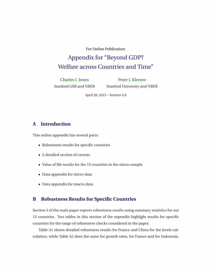
Table A1 shows detailed robustness results for France and China for the levels cal-

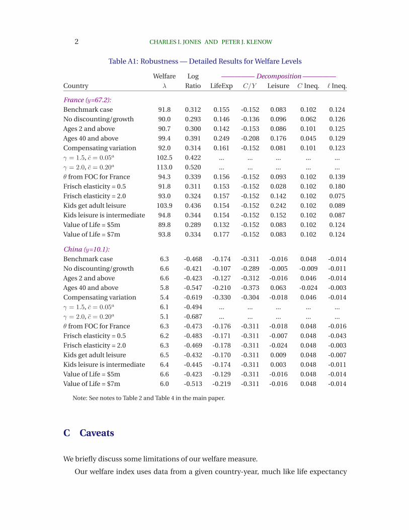
culation, while Table A2 does the same for growth rates, for France and for Indonesia.

http://stanford.edu/people/chadj

http://klenow.com/

2 CHARLES I. JONES AND PETER J. KLENOW

Table A1: Robustness — Detailed Results for Welfare Levels

Welfare Log ————— Decomposition —————

Country λ Ratio LifeExp C/Y Leisure C Ineq. ℓ Ineq.

France (y=67.2):

Benchmark case 91.8 0.312 0.155 -0.152 0.083 0.102 0.124

No discounting/growth 90.0 0.293 0.146 -0.136 0.096 0.062 0.126

Ages 2 and above 90.7 0.300 0.142 -0.153 0.086 0.101 0.125

Ages 40 and above 99.4 0.391 0.249 -0.208 0.176 0.045 0.129

Compensating variation 92.0 0.314 0.161 -0.152 0.081 0.101 0.123

γ = 1.5, c = 0.05a 102.5 0.422 ... ... ... ... ...

γ = 2.0, c = 0.20a 113.0 0.520 ... ... ... ... ...

θ from FOC for France 94.3 0.339 0.156 -0.152 0.093 0.102 0.139

Frisch elasticity = 0.5 91.8 0.311 0.153 -0.152 0.028 0.102 0.180

Frisch elasticity = 2.0 93.0 0.324 0.157 -0.152 0.142 0.102 0.075

Kids get adult leisure 103.9 0.436 0.154 -0.152 0.242 0.102 0.089

Kids leisure is intermediate 94.8 0.344 0.154 -0.152 0.152 0.102 0.087

Value of Life = $5m 89.8 0.289 0.132 -0.152 0.083 0.102 0.124

Value of Life = $7m 93.8 0.334 0.177 -0.152 0.083 0.102 0.124

China (y=10.1):

Benchmark case 6.3 -0.468 -0.174 -0.311 -0.016 0.048 -0.014

No discounting/growth 6.6 -0.421 -0.107 -0.289 -0.005 -0.009 -0.011

Ages 2 and above 6.6 -0.423 -0.127 -0.312 -0.016 0.046 -0.014

Ages 40 and above 5.8 -0.547 -0.210 -0.373 0.063 -0.024 -0.003

Compensating variation 5.4 -0.619 -0.330 -0.304 -0.018 0.046 -0.014

γ = 1.5, c = 0.05a 6.1 -0.494 ... ... ... ... ...

γ = 2.0, c = 0.20a 5.1 -0.687 ... ... ... ... ...

θ from FOC for France 6.3 -0.473 -0.176 -0.311 -0.018 0.048 -0.016

Frisch elasticity = 0.5 6.2 -0.483 -0.171 -0.311 -0.007 0.048 -0.043

Frisch elasticity = 2.0 6.3 -0.469 -0.178 -0.311 -0.024 0.048 -0.003

Kids get adult leisure 6.5 -0.432 -0.170 -0.311 0.009 0.048 -0.007

Kids leisure is intermediate 6.4 -0.445 -0.174 -0.311 0.003 0.048 -0.011

Value of Life = $5m 6.6 -0.423 -0.129 -0.311 -0.016 0.048 -0.014

Value of Life = $7m 6.0 -0.513 -0.219 -0.311 -0.016 0.048 -0.014

Note: See notes to Table 2 and Table 4 in the main paper.

C Caveats

We briefly discuss some limitations of our welfare measure.

Our welfare index uses data from a given country-year, much like life expectancy

WELFARE ACROSS COUNTRIES AND TIME 3

Table A2: Robustness — Detailed Results for Welfare Growth

————— Decomposition —————

Welfare Life Cons. Leis.

Growth Diff Exp. c/y Leisure Ineq. Ineq.

France (gy=2.15%):

Benchmark case 3.15 1.00 1.04 0.10 -0.05 -0.16 0.07

No discounting/growth 3.09 0.94 0.94 0.05 -0.05 -0.07 0.07

Ages 2 and above 3.06 0.91 0.95 0.10 -0.05 -0.16 0.07

Ages 40 and above 3.71 1.56 1.54 0.20 -0.09 -0.14 0.06

γ = 1.0, c = 0a 2.85 0.71 ... ... ... ... ...

γ = 1.5, c = 0.05a 2.74 0.60 ... ... ... ... ...

γ = 2.0, c = 0.20a 2.89 0.74 ... ... ... ... ...

θ from FOC for France 3.16 1.02 1.05 0.10 -0.06 -0.16 0.08

Frisch elasticity = 0.5 3.19 1.05 1.03 0.10 -0.01 -0.16 0.09

Frisch elasticity = 2.0 3.10 0.95 1.06 0.10 -0.10 -0.16 0.05

Kids get adult leisure 3.08 0.93 1.04 0.10 -0.13 -0.16 0.09

Kids leisure is intermediate 3.13 0.99 1.04 0.10 -0.08 -0.16 0.09

Value of Life = $5m 2.99 0.85 0.88 0.10 -0.05 -0.16 0.07

Value of Life = $7m 3.31 1.16 1.20 0.10 -0.05 -0.16 0.07

Indonesia (gy=0.39%):

Benchmark case 2.65 2.25 1.43 0.81 0.18 -0.16 -0.00

No discounting/growth 2.00 1.60 0.76 0.78 0.19 -0.12 -0.02

Ages 2 and above 2.28 1.88 1.06 0.81 0.19 -0.17 -0.01

Ages 40 and above 2.38 1.98 1.03 0.95 0.23 -0.16 -0.07

γ = 1.0, c = 0a 2.65 2.25 ... ... ... ... ...

γ = 1.5, c = 0.05a 1.59 1.20 ... ... ... ... ...

γ = 2.0, c = 0.20a 1.68 1.28 ... ... ... ... ...

θ from FOC for France 2.67 2.28 1.43 0.81 0.20 -0.16 -0.00

Frisch elasticity = 0.5 2.55 2.16 1.40 0.81 0.08 -0.16 0.03

Frisch elasticity = 2.0 2.74 2.35 1.45 0.81 0.27 -0.16 -0.02

Kids get adult leisure 2.62 2.22 1.39 0.81 0.25 -0.16 -0.07

Kids leisure is intermediate 2.58 2.19 1.43 0.81 0.16 -0.16 -0.05

Value of Life = $5m 2.21 1.82 1.00 0.81 0.18 -0.16 -0.00

Value of Life = $7m 3.08 2.69 1.87 0.81 0.18 -0.16 -0.00

Note: See notes to Table 3 and Table 4 in the main paper.

summarizes the cross-section distribution of mortality rates. It is not good at capturing

transition dynamics. To the extent consumption, leisure, or life expectancy exhibit

transition dynamics or even trend breaks (as with China after 1978), lifetime utility


could differ markedly from our snapshot. This is all the more true if individual utility

is not separable over time so that mobility in consumption and leisure matter. If an

individual or even whole economy is transitioning to a higher level of consumption,

current levels of consumption can be too pessimistic about lifetime utility. We explored

this issue in Table 8 of Jones and Klenow (2010) and noted that most observed cross-

country differences in consumption-output ratios reflect persistent (steady state) dif-

ferences rather than transition dynamics.

In a recursive world, one could take a value function approach, identifying the state

variables that matter for discounted welfare. Relevant states might include the stocks

of human and physical capital, TFP in producing final goods and health, and the de-

gree of consumption insurance.1 An advantage of this complementary value function

approach is that it might shed light on underlying policy distortions, as opposed to

simply evaluating outcomes.

We evaluate outcomes in terms of a single utility function both within and across

countries. In contrast, preference heterogeneity (at least within countries) is a routine

assumption in labor economics and public finance. See Weinzierl (2009) for a recent

discussion of how preference heterogeneity can affect optimal taxation. Although we

believe it is beyond the scope of this paper, one could try to use household data to

quantify preference heterogeneity within countries.

A related issue is whether countries differ in the efficiency of time spent in home

production. For example, human capital is surely useful at home (e.g. in childcare) as

well as in the market. To the extent the benefits take the form of future consumption,

our flow welfare index could pick this up eventually. Also, if leisure is more productive

because of a higher consumption, then this could arguably be dealt with by nonsepa-

rable momentary utility between consumption and leisure.

Our narrow utility over consumption and leisure ignores altruism, for example within

families. Given the big differences in family size and population growth rates across

countries (e.g., Tertilt (2005)), incorporating intergenerational altruism could have a

first order effect on welfare calculations.

Our measure of health focuses on the easier-to-measure extensive margin (quantity

of life), following a long tradition; see especially Nordhaus (2003). However, the inten-

1Related, Basu, Pascali, Schiantarelli and Serven (2010) suggest that total factor productivity growthmay, under quite general circumstances, be interpreted as a measure of welfare growth.


sive margin (quality of life) is obviously important as well. To the extent we include

health spending in our measure of consumption, one could argue we are capturing

the intensive margin across countries, and maybe even double-counting the extensive

margin. But this ignores differences in the natural disease environment that may cause

differences in morbidity for a given amount of health spending (e.g. the prevalence

of malaria). Moreover, in the cross-section within countries, health may be negatively

correlated with health spending (e.g. across age groups).2

Some of our parameter values implied negative flow utility for some individuals

in the poorest countries. This may understate welfare in these countries, although

negative flow utility in some periods of life is not inconsistent with positive lifetime

utility. With estimates of the value of life in some of the poorest countries, one could

get a sense for how badly this misses the mark.3 One could also incorporate hetero-

geneity in mortality rates within a country; Edwards (2010) suggests that this may be

quantitatively significant in his extension of the Becker, Philipson and Soares (2005)

growth rates.

We have neglected the natural environment more generally. The quality of the air,

water, and so on provide utility for a given amount of market consumption and leisure

and help sustain future consumption. See, for example, U.S. Bureau of Economic Anal-

ysis (1994), Dasgupta (2001) and Arrow et al. (2004).

There have been various efforts to quantify the economic costs of crime (including

prevention), such as Anderson (1999). Possibly related, Nordhaus and Tobin (1972)

subtracted urban disamenities in calculating their Measure of Economic Welfare.

The data we use for aggregate real consumption per capita is converted into dollars

using estimated PPP exchange rates. The underlying price ratios are supposed to be

for comparable-quality goods and services. But in practice it can be difficult to fully

control for quality differences, especially for education and health. And the current

methodology makes no attempt to quantify differences in variety across countries. Any

errors in the PPP exchange rate for consumption will contaminate the consumption

portion of our welfare index.

2A large recent literature also emphasizes the possible causal links between health and growth: forexample Acemoglu and Johnson (2007), Bleakley (2007), Weil (2007), Feyrer, Politi and Weil (2008), andAghion, Howitt and Murtin (2010).

3In this vein, Kremer, Leino, Miguel and Zwane (2011) use valuation of clean water in rural Kenya toestimate the implied value of averting a child death at between $769 and $3006.


Related, households in a given country may face different price indices (inclusive of

variety and quality). If so, then expenditures are not proportional to true consumption

within countries, as we have assumed. If true price indices are positively correlated

with expenditures (i.e., prices are lower in poorer areas), then the Gini coefficients we

use overstate consumption inequality.

Finally, we have not experimented with non-standard preferences such as habit

formation or keeping up with the Joneses. Doing so could imply smaller differences in

flow utility from gaps in average consumption across countries. How these alternative

preferences would affect the welfare costs of inequality is less clear.

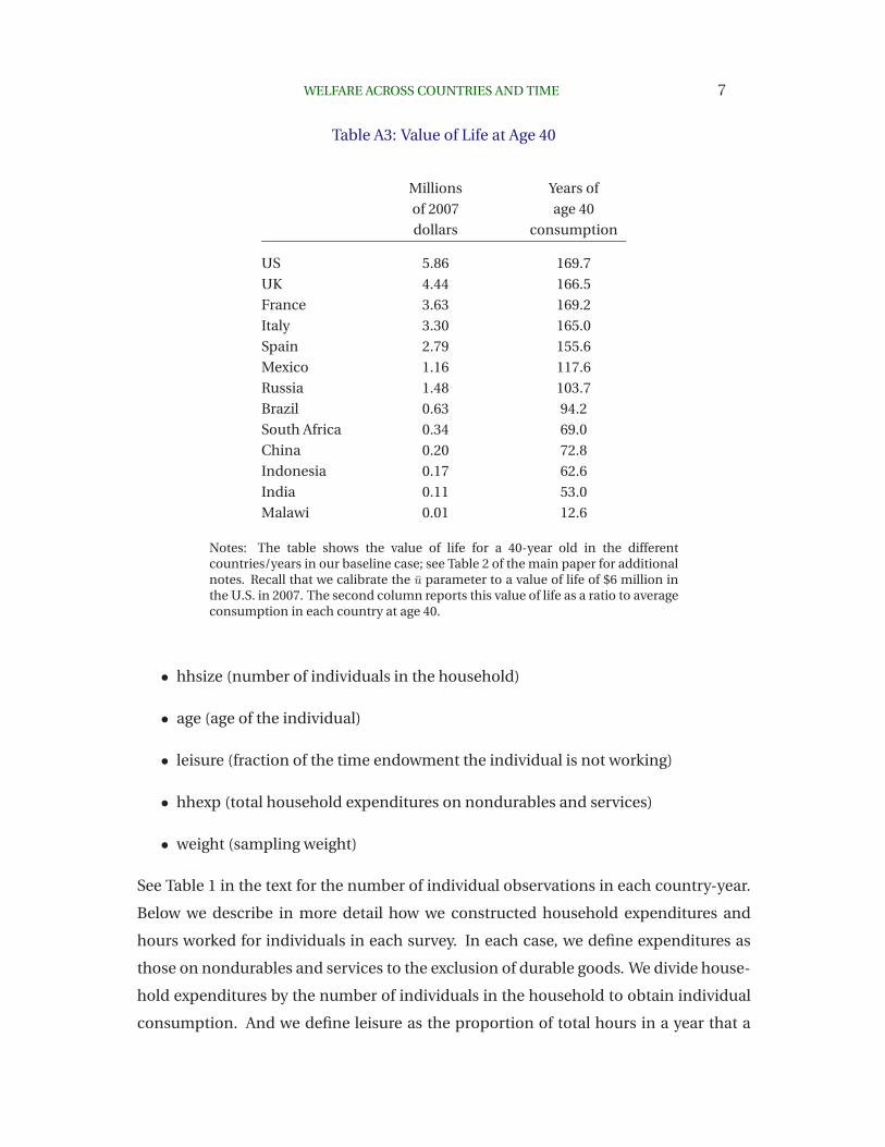
D Value of Life in Various Countries

Table A3 reports the value of life at age 40 associated with our baseline results (see Table

2 in the main paper). As is well-known, the case of log utility implies an income effect

in the value of life. For example, we find that the value of life at age 40 in the U.S. in

2006 is $5.9 million versus $1.2 million in Mexico and around $200,000 in China. As the

last column of the table shows, these differences are smaller but still important when

reported in units of “years of age 40 consumption.”

E Micro Data

E1. Overview

For the Household Survey data, we wrote two Stata programs to analyze the data for

each country-year:

• WBC YR sumstats.do

• WBC YR lamstats.do

WBC refers to the three-letter World Bank Country Code (BRA, CHN, ESP, FRA, GBR,

IDN, IND, ITA, MEX, MWI, RUS, ZAF, or USA). YR refers to the year of the survey (e.g. 06

for 2006, 85 for 1985). The “sumstats”files create datasets WBC YR.dta with the follow-

ing common set of variables for each individual covered in that household survey:

• hhid (household id code)


Table A3: Value of Life at Age 40

Millions Years of

of 2007 age 40

dollars consumption

US 5.86 169.7

UK 4.44 166.5

France 3.63 169.2

Italy 3.30 165.0

Spain 2.79 155.6

Mexico 1.16 117.6

Russia 1.48 103.7

Brazil 0.63 94.2

South Africa 0.34 69.0

China 0.20 72.8

Indonesia 0.17 62.6

India 0.11 53.0

Malawi 0.01 12.6

Notes: The table shows the value of life for a 40-year old in the differentcountries/years in our baseline case; see Table 2 of the main paper for additionalnotes. Recall that we calibrate the u parameter to a value of life of $6 million inthe U.S. in 2007. The second column reports this value of life as a ratio to averageconsumption in each country at age 40.

• hhsize (number of individuals in the household)

• age (age of the individual)

• leisure (fraction of the time endowment the individual is not working)

• hhexp (total household expenditures on nondurables and services)

• weight (sampling weight)

See Table 1 in the text for the number of individual observations in each country-year.

Below we describe in more detail how we constructed household expenditures and

hours worked for individuals in each survey. In each case, we define expenditures as

those on nondurables and services to the exclusion of durable goods. We divide house-

hold expenditures by the number of individuals in the household to obtain individual

consumption. And we define leisure as the proportion of total hours in a year that a


person does not work:

leisure =(5840− annual hours worked)

5840,

where 5840 = 365 days · 16 waking hours per day. For countries in which only “usual

weekly hours” are available, we use an estimate of the number of weeks worked from

other sources (typically the OECD), as described below. For countries in which only

the “previous week’s hours” are available, we multiply by 52 weeks per year under the

assumption that people in the survey will have been randomly taking vacation in the

previous week so that 52 is appropriate.

The “lamstats” files read in WBC YR.dta and calculate welfare relative to the U.S. in

the same year (in log differences), and its additive components due to life expectancy,

average consumption, consumption inequality, average leisure, and leisure inequality.

These calculations are made using sampling weights.

E2. Brazil

For Brazil (BRA), we use the Consumer Expenditure Survey (Pesquisa de Orcamen-

tos Familiares or POF) and the National Household Sample Survey (Pesquisa Nacional

por Amostra de Domicilios or PNAD), both of which are conducted by the Brazilian

Institute of Geography and Statistics (Instituto Brasileiro de Geografia e Estatstica or

IBGE). The POF and PNAD contain (but not limited to) information about each sur-

veyed household’s income, expenditures on final consumer goods, and demographic

characteristics. Both surveys are representative at the national level once sampling

weights are applied. We use the earliest and latest years with the necessary data, 2002-

2003 and 2008-2009, to calculate the growth rates. We use the most relevant year, 2002-

2003, for comparison with the U.S.

The PNAD and the POF have separate schedules on consumption and hours worked,

respectively, in 2002-2003 and 2008-2009. As the utility function we use in the micro

calculations is additively separable in consumption and leisure, we simply calculated

the consumption and leisure terms on the separate samples from the PNAD and the

POF in both years.

We construct consumption by adding up the reported expenditures on the follow-


ing: food, clothing, housing (rent and estimated rent for those who own their house),

utilities, communication services, medical services, transportation services, education

and cultural spending. In each case we exclude durables (furniture, durable leisure

goods, vehicles, etc.). Besides excluding the value of expenditures on durables, we ex-

clude the following: maintenance; repair and expansion of housing; deposits in savings

accounts; loans and debt payments; retirement, pensions allowance and other regular

income deductions; transfers made to acquaintances and for charity.

The PNAD contains information about typical weekly hours worked for all members

of the household aged 16 years and older. Because the survey does not ask about weeks

worked in the year and Brazil is not one of the OECD countries, we use the OECD

statistics for the average of the weeks worked per worker across OECD countries: 45.8

weeks in 2003 and 45.4 weeks in 2008. For those in the household under 16 years old,

we assume zero hours worked so that their fraction of leisure time is 1.

E3. China

For China we use the Chinese Household Income Project (CHIP) survey conducted

by the Rural Survey Group of the National Bureau of Statistics of China and by the

Institute of Economics of the Chinese Academy of Social Science. The CHIP covers

both rural and urban areas of China. The datasets contain (but not limited to) each sur-

veyed household’s income, expenditures on final consumer goods, and demographic

characteristics. The survey is a repeated cross section, conducted every seven years

since 1988, and considered to be self-weighted. Because the 1988 and 1995 surveys did

not include information about hours worked per week, and the 2007 survey is not yet

available, we only use the 2002 CHIP.

We construct consumption for urban and rural households by adding up the re-

ported expenditures on the following: food, clothing, housing (rent and estimated rent

for those who own their house), utilities, communication services, medical services,

transportation services, education and cultural spending. In these categories we in-

clude estimated home production for self-consumption and gifts received. In each case

we exclude durables (furniture, durable leisure goods, vehicles, etc.). Besides excluding

expenditures on durables, we exclude the following: maintenance, repair and expan-

sion of housing; spending on family business and agricultural production, deposits in


savings accounts; loans and debt payments; income and property taxes; purchases of

land, houses or condominiums; and transfers made to acquaintances and for charity.

One drawback of the CHIP data is that it lacks rent information for rural households. To

impute rent in rural areas, we use the average rent over value ratio for houses in urban

areas and apply the urban ratio to the value of each house in a rural area.

The urban dataset contains information about monthly hours worked and number

of months employed for all members of the household aged 16 years and older. For

rural residents, we construct hours worked by adding up the reported hours worked in

planting, raising livestock and non-agriculture jobs. For those in the household under

16 years old, we assume zero hours worked so that their fraction of leisure time is 1.

E4. Spain

For Spain (ESP), we used the European Community Household Panel (ECHP) carried

out by the European Commission and the Encuesta Continua de Presupuestos Famil-

iares (ECPF) Base 1997 carried out by the Instituto Nacional de Estadstica. The ECPF

is a quarterly survey that contains information about household expenditures and de-

mographic characteristics for a panel of households. The Base 1997 survey is available

for the years 1998-2005. The ECHP is a panel survey and contains information about

employment and demographic characteristics for the years 1994-2001. We use the

latest year with both consumption and leisure data, 2001, for comparison with the U.S.

Our measure of consumption includes reported expenditures on the following: food

and beverages, clothing and footwear, housing, water, electricity, gas and other fuels,

health (medical services, drugs, etc), transportation services, communications (postal

services, telephone, telegraph, and fax services), leisure and entertainment, education

services, hotels, cafes and restaurants, personal care (hairdressing etc), social protec-

tion, insurance and other financial services. We exclude spending on durable goods

(furniture, appliances, vehicles etc) as well as spending on the maintenance and repair

of the house and other durable goods, and remittances to non-resident household

members. We use the average annual consumption over the four quarters of the ECPF.

The ECHP dataset contains information about the total number of hours work-

ing per week in main and additional jobs for household members aged 16 and over.

Because the survey does not ask about weeks worked in the year, we assume those


working work 43.1 weeks, as in the 2001 OECD statistics for Spain. For those in the

household under 16 years old, we assume zero hours worked so that their fraction of

leisure time is 1.

E5. France

For France (FRA) we use the Family Budget Survey (Enquete Budget de Famille - or

EBF) conducted by the National Institute for Statistics and Economic Studies. The

EBF contains information about each surveyed household’s income, expenditures on

final consumer goods, and demographic characteristics. The survey is a repeated cross

section, conducted every five years since 1979, and is representative at the national

level once sampling weights are applied. We use the earliest and latest years with the

necessary data, 1984 and 2005, to calculate growth rates. We use the latest year, 2005,

for comparison with the U.S. We construct consumption by adding up the reported

expenditures on the following: food, clothing, utilities (payments for electricity, etc),

accessories for the house (e.g., dishes, cooking utensils, light bulbs) excluding furni-

ture, medical services, communication services (e.g., postal and telephone services),

leisure and cultural spending (expenditures on pets, gardening, theater tickets, and

entertainment events), accessories for personal care (soaps, perfumes, brush, etc.),

professional services (lawyers, accountants, funerals, etc.), and transportation services

(bus or subway tickets, taxi fees, etc.). In each case we exclude durables (furniture,

durable leisure goods, vehicles, etc.). Besides excluding the value of expenditures on

durables, we exclude the following: maintenance; repair and expansion of housing;

deposits in savings accounts; loans and debt payments; income and property taxes;

purchases of land, houses or condominiums; transfers made to acquaintances and for

charity; and value of items stolen. The dataset contains information about weekly

hours worked for all members of the household aged 16 years and older. Because

the household survey does not ask about weeks worked in the year, we use the OECD

statistics for weeks worked per worker in France: 43.5 weeks in 1984 and 41.0 weeks in

2005. For those in the household under 16 years old, we assume zero hours worked so

that their fraction of leisure time is 1.


E6. U.K.

For the United Kingdom (GBR), we use the Family Expenditure Survey (FES) conducted

by the Office for National Statistics. The FES contains information about each surveyed

household’s income, expenditures on final consumer goods, and demographic charac-

teristics. The survey is a repeated cross section, conducted annually since 1957, and

is representative at the national level once sampling weights are applied. We use the

earliest and latest years with the necessary data, 1985 and 2005, to calculate growth

rates. We use the latest year, 2005, for comparison with the U.S.

We used a cleaned version of the FES data generously made available by Richard

Blundell and Ben Etheridge, following their methodology in Blundell and Etheridge

(2010). As a result we apply their definitions of consumption expenditures and hours

worked. Specifically, we start from their definition of non-durable goods (food, cater-

ing, alcohol, tobacco, fuel, household services, clothing, personal goods and services

motoring expenses excluding vehicle purchases, travel expenses, leisure goods exclud-

ing audiovisual equipment, entertainment and holiday expenses) and add the real hous-

ing cost. We exclude durables expenditures.

The FES contains information about weekly hours worked for all members of the

household aged 16 years and older. Because the survey does not ask about weeks

worked in the year, we use the OECD statistics for weeks worked per worker in the

nearest year in United Kingdom: 45.4 weeks in 1987 and 45.1 weeks in 2005. For those

in the household under 16 years old, we assume zero hours worked so that their fraction

of leisure time is 1. As the survey lumps children whose ages are 15 and below together,

we assume they are equally distributed between age 1 and age 15 (inclusive).

E7. India

For India (IND) we use the National Sample Survey (NSS) conducted by the Indian

Ministry of Statistics and Programme Implementation. In some rounds (years) the NSS

contains information about expenditures on final consumer goods and demographic

characteristics for a cross-section of households. We use the earliest and latest years

with the necessary data, 1983-1984 and 2004-2005, to calculate growth rates. We use the

latest year, 2004-2005, for comparison with the U.S. The 1983-1984 survey has separate

schedules on consumption and time use, respectively. We were able to plausibly match


roughly one-half of the households in the two schedules. The relevant statistics (con-

sumption and leisure levels and inequality by age) are similar whether we use only the

matched households or all households. As the utility function we use in the micro cal-

culations is additively separable in consumption and leisure, we simply calculated the

consumption and leisure terms on the separate samples in 1983-1984. The 2004-2005

survey covered both consumption and leisure for a common set of households. Our

measure of consumption includes expenditures on the following, which the survey asks

about specifically: food (itemized), fuel and light, cinema/theater/video, tuition fees,

newspapers/magazines/fiction, medical expenses, toilet articles, regular (commuting

type) and other journeys, house rent, clothing and footwear. Respondents were asked

to include the value of home production consumed in these categories. We exclude

spending on durable goods, which were also asked about and itemized (furniture, ap-

pliances, etc.). The dataset contains “daily time disposition” for the prior seven days

for each household member. For each day, two main activities were identified and

recorded. We count the following as working: self-employment, unpaid family labor,

regular salary/wage employment, and casual wage labor. The survey asks the respon-

dent to assign each activity a “full-intensity” (4 hours or more) or a “half-intensity” (1-4

hours). For constructing hours worked in a week, we treat full-intensity as 8 hours and

half-intensity as 2.5 hours for the first 5 days of the week, and half these levels for days

6 and 7. With these values, many individuals work the resulting maximum of 48 hours

in a week in the Indian survey. We multiply weekly hours worked by 52 weeks to get

annual hours worked, as the prior seven days should include weeks not worked. As

these conversions are admittedly arbitrary, however, the Indian leisure results must be

taken with particular caution.

E8. Indonesia

For Indonesia (IDN), we use the National Socioeconomic Surveys (SUSENAS) for 1993

and 2006 conducted by the Central Bureau of Statistics. This survey contains detailed

information about each household’s expenditures and demographic characteristics and

includes sampling weights.

We construct consumption by adding up reported expenditures on the following:

food, housing, fuel, lighting, education, health, clothing, and miscellaneous goods and


services. We exclude expenditures on durables (household appliances, vehicles, jew-

elry etc.).

The SUSENAS survey contains information about weekly hours worked in the pre-

vious week for all members of the household aged 10 years and older. The survey does

not ask about weeks worked in the year, so we multiply by 52 weeks to get annual hours

worked. For people under the age of 10, we set hours worked to zero, so their fraction

of leisure time is 1.

E9. Italy

For Italy (ITA) we use the Survey of Household Income and Wealth (SHIW) conducted

by the Bank of Italy. The SHIW contains detailed information about each household’s

expenditures and demographic characteristics. The survey is a repeated cross section,

conducted annually from 1965 to 1987 (with the exception of 1985), and every other

year since 1987 (with the exception of a three-year interval between 1995 and 1998).

Information on hours and other dimensions of labor supply are available from 1987. It

is representative at the national level once sampling weights are applied. We use the

earliest and latest years with the necessary data, 1987 to 2006, to calculate growth rates.

We use the latest year, 2006, for comparison with the U.S.

We use a cleaned version of the SHIW data generously made available by Tullio

Jappelli and Luigi Pistaferri, used in Jappelli and Pistaferri (2010). Our measure of

consumption includes expenditures on the following: housing (rent and estimated rent

for those who own their house), other services, and non-durable goods. The survey

question on non-housing consumption instructs the respondent to exclude the fol-

lowing categories (mostly durables): purchases of precious objects; purchases of cars;

purchases of household appliances and furniture; extraordinary maintenance of your

dwelling; life insurance premiums; and contributions to private pension funds.

The SHIW contains information about average weekly hours worked during the year

(as an employee or self-employed) for the respondent and for other family members 16

years old and older (spouse, son/daughter, etc.). It also contains months worked in the

year. For those in the household under 16 years old, we set hours worked to zero, so

their fraction of leisure time is 1.


E10. Malawi

For Malawi (MWI) we use the 2004 Integrated Household Survey (IHS) conducted by

the National Statistics Office. The survey contains information about each surveyed


teristics.

We construct consumption by taking the real annual household consumption ex-

penditure aggregate in the auxiliary file of the dataset and subtracting from it furnish-

ings, vehicles and major recreational durables. The resulting consumption measure

includes expenditures on the following: food items, alcohol and tobacco, clothing,

housing and utilities, health, transport services, communication, recreation, educa-

tion, vendors and cafes, and other services.

The data contains information for all individuals 5 years or older on hours spent

on household activities, collecting water and collecting firewood, hours spent on agri-

cultural activities, household business, casual or daily (ganyu) labour, and salaried

employment. The survey reports the number of hours spent on household business

and agriculture in the week before the survey. We convert this to an annual value

by multiplying by 52, as the week before should include weeks not worked for some

individuals. We exclude hours spent on collecting water and firewood because values

for these items are not available for inclusion in our consumption measure. For indi-

viduals who were employed in full time or part time jobs during the past 12 months, we

compute annual hours worked by multiplying the reported weeks or months of work

by the reported average days worked in a month and reported average hours worked

per day.

E11. Mexico

For Mexico we use the National Survey of Household Income and Expenditure (En-

cuesta Nacional de Ingresos y Gastos de los Hogares - or ENIGH) conducted by the

National Institute of Statistics and Geography. ENIGH contains information about each

surveyed household’s income, expenditures on final consumer goods, and demographic

characteristics. The survey is a repeated cross section, conducted every two years,

and it is representative at the national level once sampling weights are applied. We

use the earliest and latest years with the necessary data, 1984 and 2006, to calculate


growth rates. We use the latest year, 2006, for comparison with the U.S. Our measure

of consumption includes expenditures on the following: housing (rent and estimated

rent for those who own their house), food, clothing and accessories, household services

(e.g. utilities), accessories for the house (e.g., light bulbs) excluding furniture, leisure

spending (expenditures on pets, gardening, and entertainment events), accessories for

personal care (soaps, perfumes, brush, etc.), professional services (lawyers, accoun-

tants, funerals, etc.), and transportation services (bus or subway tickets, taxi fees, etc.).

In these categories we include estimated home production for self-consumption and

gifts received. In each case we exclude durables (furniture, durable leisure goods, ve-

hicles, etc.). Besides excluding the value of expenditures on durables, we exclude the

following: maintenance, repair and expansion of housing; deposits in savings accounts;

loans and debt payments; income and property taxes; purchases of land, houses or

condominiums; transfers made to acquaintances and for charity; and value of items

stolen. The dataset contains information about weekly hours worked (in the previous

month) for all members of the household aged 12 years and older. Because the survey

does not ask about weeks worked in the year, we use the OECD statistics for weeks

worked per worker in the nearest year in Mexico (41.4 weeks worked in 1991 and 43.2

in 2004). For those in the household under 12 years old, we assume zero hours worked

so that the fraction of leisure time is 1 for them.

E12. Russia

For Russia, we use the Russia Longitudinal Monitoring Survey (RLMS) organized by the

Population Center at the University of North Carolina in cooperation with the Russian

Academy of Sociology. The RLMS contains information about each surveyed house-

hold’s income, expenditures on final consumer goods, and demographic characteris-

tics. The survey is a repeated cross section and is representative at the national level

once sampling weights are applied. We use the earliest and latest years with the neces-

sary data, 1998 and 2007, to calculate growth rates. We use 2006 for comparison with

the U.S.

Our measure of consumption includes reported expenditures on the following: food

and beverages, clothing and footwear, housing services, water, electricity, gas and other

fuels, health (medical services, drugs, etc.), transportation services, communications


(postal services, telephone, telegraph, and fax services), leisure and entertainment, ed-

ucation services, hotels, cafes and restaurants, personal care (hairdressing etc.), social

protection, insurance and other financial services. We exclude spending on durable

goods (furniture, appliances, vehicles etc.) as well as spending on the maintenance

and repair of the house and other durable goods.

The RLMS contains information about weekly hours worked for all members of

the household aged 16 years and older. Because the survey does not ask about weeks

worked in the year, we use the OECD statistics for Russia: 44.9 weeks in 1998, 44.1 weeks

in 2006, and 44.4 weeks in 2007. For those in the household under 16 years old, we

assume zero hours worked so that their fraction of leisure time is 1.

E13. South Africa

For South Africa we use the Integrated Household Survey (HIS) conducted by the South

Africa Labour Development Research Unit (at the University of Cape Town) in col-

laboration with the World Bank. The HIS contains information about each surveyed


teristics. The survey is a single cross section, conducted from mid-1993 through early

1994. Our measure of consumption includes expenditures on the following: housing

(rent and estimated rent for those who own their house), utilities, food, personal items,

clothing, health care, schooling, and transportation. The survey explicitly asks about

food consumption from own production. We exclude durables expenditures (including

home repairs). The dataset contains information about monthly hours worked for all

members of the household aged 16 years and older. Workers include the self-employed,

those employed in a family business (including crop production for own consumption),

those with regular employment, and those with casual or temporary employment. We

multiply monthly hours worked by 12 months to get annual hours worked. For those in

the household under 16 years old, we assume zero hours worked so that the fraction of

leisure time is 1 for them.

E14. United States

For the U.S. we used the Consumer Expenditure Survey (CES) carried out by the U.S.

Bureau of Labor Statistics. The CES contains information about each surveyed house-


hold’s income, expenditures on final consumer goods, and demographic characteris-

tics. The survey is a rotating panel of households, with each household reporting ex-

penditures and hours worked for up to four consecutive quarters. We use various years

from 1984 through 2006 for comparison with other countries (e.g. South Africa in 1993),

and for calculating U.S. growth rates from 1984-2006. We use a cleaned version of the

CES data generously made available by Dirk Krueger and Fabrizio Perri, following their

methodology in Krueger and Perri (2006). As a result we use their definitions of con-

sumption expenditures and hours worked. Specifically, we start from their definition

of nondurables (food, personal care, fuel, utilities, household operations, public trans-

portation, apparel, education, reading, health services, and miscellaneous personal

services) and add the following: services from vehicles, other vehicle expenses, services

from owned primary residence, rent, other lodging expenditures, and entertainment.

We exclude durables expenditures. The CES contains information about weeks worked

and hours per week for the respondent and for the respondent’s spouse (if any). For

other members of the household, we assumed zero hours worked so that the fraction

of leisure time is 1. As the survey lumps children 15 and under (other than babies)

together, we assume they are equally distributed between age 2 and age 15 (inclusive).

F Macro Data

The basic data sources that we use and an overview of the manipulations of this data are

described in the main paper in Section 6. Some of the basic underlying data that goes

into our calculations is available in the spreadsheet where we report our extended re-

sults; that file is available at http://www.stanford.edu/∼chadj/BeyondGDP400.xls. Once

we’ve double-checked and better annotated our matlab and stata programs, these will

be made available. If you’d really like to see the programs immediately, send us an email

and we’ll be happy to provide them.

The file “BeyondGDP-ReplicationInstructions.txt” contained in “BeyondGDP-ReplicationFiles.zip”

contains further details about the programs and how to replicate the results. The re-

mainder of this section provides more details about the underlying data we use.

http://www.stanford.edu/~chadj/BeyondGDP400.xls


F1. Programs for Reading and Cleaning Data

WIID3aLevels80.m, WIID3aGrowth80.m: These programs read and clean the WIID

data on Gini coefficients. The source for our inequality data is the UNU-WIDER World

Income Inequality Database, Version 3.0a, dated June 2014 and available at

http://www.wider.unu.edu/research/WIID-3a/en GB/database/. The WIID database

reports income and consumption Gini coefficients from a variety of micro data sets

for many countries and years. We use consumption measures when they are avail-

able and infer consumption measures from disposable income measures when only

the latter are available. For the cross-sectional analysis, we average across available

observations that meet a certain quality threshhold for the 3 observations available

since 2000 that are closest to our reference year, 2007. For the time-series analysis,

we use data from the 3 years closest to 1980 from the period 1975–1985 and from the 3

years closest to 2007 since 2000 for the 2007 estimate. LifeExpectancyWB80.m: Loads

the life expectancy data from the World Bank. These data are taken directly from the

World Bank’s HNPStats database.4 WBAdultPopulation80.m: We measure time spent

in leisure or home production as the difference between a time endowment and time

spent in employment. Our measure of time engaged in market work aims to capture

both the extensive and intensive margins. For the extensive margin, the Penn World

Tables, Version 8.0 provides a measure of employment. We divide this employment

measure by the adult population, i.e. those ages 15 and over (obtained from the World

Bank). The program WBAdultPopulation.m loads the fraction of the population aged

15 and over.

AnnualHoursPWT80.m Our measure of the intensive margin is annual hours worked

per person. We use the “avh” series from PWT 8.0 to measure hours, which is primarily

available for OECD countries. Missing values are set equal to the U.S. value.

References

Acemoglu, Daron and Simon Johnson, “Disease and development: the Effect of Life Expectancy

on Economic Growth,” Journal of Political Economy, 2007, 115 (6), 925–985.

Aghion, Philippe, Peter Howitt, and Fabrice Murtin, “The Relationship Between Health and

Growth: When Lucas Meets Nelson-Phelps,” NBER Working Paper 15813 March 2010.

4See http://go.worldbank.org/N2N84RDV00, series code SP.DYN.LE00.IN.

http://www.wider.unu.edu/research/WIID-3a/en_GB/database/

http://go.worldbank.org/N2N84RDV00


Anderson, David A., “The Aggregate Burden of Crime,” Journal of Law and Economics, October

1999, 42, 611–642.

Arrow, Kenneth, Partha Dasgupta, Lawrence Goulder, Gretchen Daily, Paul Ehrlich, Geoffrey

Heal, Simon Levin, Karl-Goran Maler, Stephen Schneider, David Starrett, and Brian Walker,

“Are We Consuming Too Much?,” Journal of Economic Perspectives, Summer 2004, 18 (3), 147–

172.

Basu, Susanto, Luigi Pascali, Fabio Schiantarelli, and Luis Serven, “Productivity, Welfare and

Reallocation: Theory and Firm Level Evidence,” Boston College manuscript June 2010.

Becker, Gary S., Tomas J. Philipson, and Rodrigo R. Soares, “The Quantity and Quality of Life and

the Evolution of World Inequality,” American Economic Review, March 2005, 95 (1), 277–291.

Bleakley, Hoyt, “Disease and Development: Evidence from Hookworm Eradication in the

American South,” The Quarterly Journal of Economics, February 2007, 122 (1), 73–117.

Dasgupta, Partha, Human Well-Being and the Natural Environment, Oxford and New York:

Oxford University Press, 2001.

Edwards, Ryan D., “The Cost of Uncertain Life Span,” Queen’s College manuscript May 2010.

Feyrer, James., Dimitra Politi, and David N. Weil, “The Economic Effects of Micronutrient De-

ficiency: Evidence from Salt Iodization in the United States,” manuscript, Brown University,

2008.

Jones, Charles I. and Peter J. Klenow, “Beyond GDP: Welfare across Countries and Time,”

September 2010. NBER Working Paper 16352.

Kremer, Michael, Jessica Leino, Edward Miguel, and Alix Peterson Zwane, “Spring Cleaning:

Rural Water Impacts, Valuation and Property Rights Institutions,” Quarterly Journal of

Economics, February 2011, 126 (1), 145–205.

Krueger, Dirk and Fabrizio Perri, “Does Income Inequality Lead to Consumption Inequality?

Evidence and Theory,” Review of Economic Studies, January 2006, 73 (1), 163–193.

Nordhaus, William D., “The Health of Nations: The Contribution of Improved Health to Living

Standards,” in Kevin M. Murphy and Robert Topel, eds., Measuring the Gains from Medical

Research: An Economic Approach, Chicago: University of Chicago Press, 2003, pp. 9–40.

and James Tobin, “Is Growth Obsolete?,” in “Economic Research: Retrospect and Prospect

Vol 5: Economic Growth,” National Bureau of Economic Research, Inc, December 1972,

pp. 1–80.


Tertilt, Michele, “Polygyny, Fertility, and Savings,” Journal of Political Economy, 12 2005, 113 (6),

1341–1371.

U.S. Bureau of Economic Analysis, “Integrated Economic and Environmental Satellite Ac-

counts,” Survey of Current Business, April 1994, 74, 33–49.

Weil, David N., “Accounting for The Effect of Health on Economic Growth,” Quarterly Journal

of Economics, 2007, 122 (3), 1265–1306.

Weinzierl, Matthew, “Incorporating Preference Heterogeneity into Optimal Tax Models: De

Gustibus non est Taxandum,” May 2009. unpublished paper, Harvard University.

Documents

For OnlinePublication: Appendix for“Beyond GDP? Welfare