FNCE 3020Financial Markets and Institutions Lecture 6; Part 1

Expectations and Financial Markets(The Efficient Market Hypothesis)

Objectives for This Lecture Series (1) To discuss the role of expectations in financial

markets.How do expectations influence asset prices and decisions

of investors and borrowers in the financial markets.

(2) To introduce you to the concept of market efficiency and the Efficient Market Hypothesis.

(3) To introduce you to the controversy surrounding the Efficient Market Hypothesis.

The Role of Expectations Expectations play a critical role in financial markets.

Here are some examples: Expectations about inflation affect

Interest rates in the bond market. Central Bank actions.

Expectations about interest rates affect The term structure of interest rates, i.e. the slope of the

yield curve The movement stock and bond prices and foreign

exchange rates. Expectations about future economic activity affect

Bond and stock prices.

Adaptive Expectations Model Key issue: How are “expectations” formed? Prior to the 1960s, most economists assumed that

market participants formed adaptive expectations. Their expectations about a variable were based on past

values of that variable, and changed slowly over time. There were, however, a couple of problems with

this adaptive model of expectations: A particular variable may be affected by many other

variables, so people will likely use all relevant data in forming an expectation about a variable (not just the variable itself).

Expectations can change very quickly if the environment also experiences sudden, substantial changes.

Abrupt Change in 1970s/1980s Environment Affecting Expectations

The New Environment for Bonds

Rational Expectations Model As a result of the issues surrounding the adaptive

expectations model, a more realistic model of expectations, called rational expectations, was introduced: According to this model, expectations are formed

using all available information. Rational expectations results in the market making its

“best forecast” (optimal forecast) given available information.

However – and this is important -- it is still a forecast, it could be wrong, and will be wrong if expectations about the future turn out to be incorrect.

Rational Expectations and Efficient Financial Markets Applying the theory of rational expectations to

financial markets produces the “efficient markets theory.” The efficient markets theory assumes that asset prices

reflect all available information (events) that directly impact on the future cash flow of a security (financial asset):

This includes: Past events, Current events and Expected future events.

Based upon all available information, the market forms its expectations and then sets prices accordingly.

Efficient Market Theory (Hypothesis) and Stock Prices Application of Efficient Market Theory to common

stocks can be traced to the work of Eugene Fama (1965, Financial Analyst Journal) For an interview with Fama see: http://

www.dfaus.com/library/reprints/interview_fama_tanous/ Efficient market theory: Stocks are always correctly

priced since everything that is publicly known about a stock is reflected in its market price.

Random walk theory: All future price changes are independent from previous price changes, thus, future stock prices cannot be predicted. See: A Random Walk Down Wall Street, by Burton Malkiel

(Norton Publishing 1973).

The Efficient Market Hypothesis (EMH) According to Eugene Fama Quoting Eugene Fama: “In an efficient market, competition among the many

intelligent participants leads to a situation where, at any point in time, the actual prices of securities already reflects the effects of information based on events that have

(1) already occurred and on events, (2) as of now, [and events] (3) the market expects to take place in the future.”

Eugene F. Fama, "Random Walks in Stock Market Prices," Financial Analysts Journal, September/October 1965

Role of Unexpected Events According to Eugene Fama’s definition of efficient

markets, financial asset prices reflect the best knowledge of the past, the present and predictions of the future.

Key issues: What happens when something unexpected occurs? How does the market react if the market is efficient? How does the market react if the market is inefficient? How quickly do asset prices adjust? How does an efficient market react to anticipated events? How does an inefficient market react to anticipated events?

Next two slides illustrating addressing these questions from Nikolai Chuvakhin, “Efficient Market Hypothesis and Behavioral Finance – Is a Compromise in Sight?”

Fama’s Illustration of Market’s Reaction to Unanticipated Events

Fama’s Illustration of Market’s Reaction to Anticipated Events

Example: Krispy Kreme and the Efficient Market Theory Founded in 1937 (in Winston-Salem, NC) , the company went

public (IPO) on April 5, 2000 and traded on NASDAQ. The company listed on the NYSE on May 17, 2001. The company was selling over 7.5 million doughnuts a day. Earnings announcement: Monday, November 22, 2004 (prior to

the opening on the NYSE) for the three months ending October 31, 2004. Analysts had expected Krispy Kreme to earn 13 cents per share, Instead, the company announced its first quarterly loss since

going public in 2000. Losses for the three months ending Oct. 31 were $3 million, or 5

cents per share, down from a profit of $14.5 million, or 23 cents per share, a year earlier.

Announced earnings (loss) were not in line with market expectations. So, what happened to the stock?

Krispy Kreme: Monday, November 22, 2004; Reaction to Unexpected Event

Example: Stock Market Reacts to Fed Surprise On Tuesday, September 18, 2007, the Federal Reserve surprised

financial markets by lowering the fed funds rate 50 basis points to 4.75% (the markets had been anticipating a reduction of 25 basis points). The announcement took place at 2:15EST.

Testing the Efficient Market Hypothesis The EMH provided the theoretical basis for much of the

financial market research during the 1970s and 1980s. During that time, most of the evidence seems to have

been consistent with the EMH. Prices were seen to follow a random walk model and the

predictable variations in equity returns, if any, were found to be statistically insignificant.

So, most of the studies in the 1970s focused on the inability to predict prices from past prices.

However, beginning in the 1980s, the EMH became somewhat controversial, especially after the detection of certain anomalies in the capital markets (i.e., situations which provided “abnormal returns”).

Testing for Financial Market Anomalies Some of the main financial market anomalies

that have been identified are as follows: 1. The January Effect: Rozeff and Kinney (1976)

were the first to document evidence of higher mean stock returns in January as compared to other months.

The January effect has also been documented for bonds by Chang and Pinegar (1986).

Maxwell (1998) showed that the bond market effect is strong for non-investment grade bonds, but not for investment grade bonds.

The Weekend (or Monday) Effect 2. The Weekend Effect (or Monday Effect):

French (1980) analyzed daily returns of U.S. stocks for the period 1953-1977 and found that there was a tendency for returns to be negative on Mondays whereas they were positive on the other days of the week.

Agrawal and Tandon (1994) found significantly negative returns on Monday in nine countries and on Tuesday in eight countries, yet large and positive returns on Friday in 17 of the 18 countries studied.

Steeley (2001) found that the weekend effect in the UK disappeared in the 1990s.

Seasonal Effects

3. Seasonal Effects: Holiday and turn of the month effects have been documented over time and across countries.

Lakonishok and Smidt (1988) showed that U.S. stock returns were significantly higher at the turn of the month, defined as the last and first three trading days of the month.

Ziemba (1991) found evidence of a turn of month effect for Japan when turn of month was defined as the last five and first two trading days of the month.

Cadsby and Ratner (1992) provided evidence to show that returns were, on average, higher the day before a holiday, than on other trading days.

Small Firm Effects

4. Small Firm Effect: Banz (1981) published one of the earliest

articles on the 'small-firm effect' which is also known as the 'size-effect'. His analysis of the 1936-1975 period in the U.S.

revealed that excess returns would have been earned by holding stocks of low capitalization companies.

Over/Under Reaction Effect 5. Over/Under Reaction of Stock Prices to

Earnings Announcements: DeBondt and Thaler (1985, 1987) presented evidence that is consistent with stock prices overreacting to current changes in earnings. They reported positive (negative) estimated

abnormal stock returns for portfolios that previously generated inferior (superior) stock price and earning performance.

This was construed as the prior period stock price behavior overreacting to earnings announcements.

Standard and Poor’s Effect

6. Standard & Poor’s (S&P) Index effect: Harris and Gurel (1986) and Shleifer (1986) found an increase in share prices (up to 3 percent) on the announcement of a stock's inclusion into the S&P 500 index. Since in an efficient market only new information

should change prices, the positive stock price reaction appears to be contrary to the EMH because there is no new information about the firm other than its inclusion in the index.

Weather Effect

7. The Weather: Saunders (1993) showed that the New York Stock Exchange index tended to fall when it was cloudy.

Hirshleifer and Shumway (2001) analyzed data for 26 countries from 1982-1997 and found that stock market returns were positively correlated with sunshine in almost all of the countries studied.

Volatility Effect 8. Volatility Effect: These tests are designed to test

for rationality of market behavior by examining the volatility of share prices relative to the volatility of the fundamental variables that affect share prices.

Shiller (1981) and LeRoy and Porter (1981) showed that fluctuations in actual prices (for both stocks and bonds) were greater than those implied by changes in fundamental variables during volatile periods.

Schwert (1989) found increased volatility in financial asset returns during recessions. The empirical evidence provided by volatility tests suggests

that movements in stock prices cannot be attributed merely to the rational expectations of investors, but also involve an irrational component.

Volatility Effect: October 19, 1987 On October 19, 1987, the stock market plunged with what, on

that day, was the largest one-day point loss in the history of the Dow Jones Industrial Average (507.99 points, or 22.6%). Issue: Could such a large one-day loss be reconciled with

efficient markets and the data at that time? The were several factors justifying lower stock prices at the

time: widening federal budget, trade deficits, legislation against corporate takeovers, rising inflation, and a falling dollar.

However, none of these fundamentals experienced such a dramatic one-day change as to precipitate the 22.6% decline. Many economists concluded that this episode is evidence

that investor psychology plays a role in setting stock prices (along with the fundamentals).

Lead to the study of Behavioral Finance

Human Behavior in Markets If we assume that markets are not totally rational

(i.e., they don’t react as a rational expectations model would suggest), it might be possible to explain some of the anomaly findings on the basis of human and social psychology. John Maynard Keynes once described the stock market as

a "casino" guided by "animal spirit" (1939). Shiller (2000) describes the rise in the U.S. stock market in

the late 1990s as the result of “psychological contagion leading to irrational exuberance.”

Behavioral Finance and Asset Pricing Suggests that real people:

Have limited information processing capabilities Exhibit systematic bias in processing information Are prone to making mistakes Tend to rely on the opinion of others (fads); referred to

as a “bandwagon” effect.

Conclusions from EMH Tests The studies based on EMH have made an

invaluable contribution to our understanding of financial market. The role of information (especially new information) in

asset pricing. However, for some there seems to be growing

discontentment with the theory’s “rational expectations” focus.

However, for an excellent paper in support of the EMH read: “The Efficient Market Hypothesis and its Critics,” by Burton Malkiel, Princeton University, Working Paper #91, April 2003.

Appendix 1: Impacts of Unexpected Events on Asset Prices

The following are examples of unanticipated events and their impacts on various asset prices.

Nike Reacts to Surprise Announcement Thursday, November 18, 2004  Near the close of the market (just before 4:00) the

company announced that Philip H. Knight, co-founder of Nike (NYSE: NKE) Inc., was stepping down as president and chief executive officer of the company.

Stock Market Reacts to Fed Surprise On Tuesday, September 18, 2007, the US Federal Reserve

surprised financial markets by lowering the fed funds rate 50 basis points to 4.75% (the markets had been anticipating a reduction of 25 basis points). The Fed announcement took place at 2:15EST.

Foreign Exchange Reaction to Fed Surprise On Tuesday, September 18, 2007, the US Federal Reserve

surprised by financial markets by lowering the fed funds rate 50 basis points to 4.75% (the markets had been anticipating a reduction of 25 basis points). The Fed announcement took place at 2:15EST.

Appendix 2: Over-Reaction Effect

Case Study: Nike and the Over Reaction Effect

Nike and the Overreaction Effect Thursday, November 18, 2004  Near the close of the market (just before 4:00) the

company announced that Philip H. Knight, co-founder of Nike (NYSE: NKE) Inc., was stepping down as president and chief executive officer of the company.

Overreaction of Nike Stock

Close Day Before $85.99 (11/17)

Close Day Of $85.00 (11/18) % change* -1.2%

Close the Day After: $82.50 (11/19) % change* -4.1%

Close 7 Days After $86.55 (12/1) % change** = 4.9%

Note: * = % change from close day before announcement.

** = % change from close the day after the announcement.

Appendix 3: Three Forms of Market Efficiency

The following slides discuss the three forms of market efficiency and the use of forecasting with these three forms.

Three Forms of The Efficient Market Hypothesis

There are actually three stages of the EMH model: Weak Form: Current prices reflect all past price and past

volume information. The fundamental information contained in the past sequence of

prices of a security is fully reflected in the current market price of that security.

Semi-strong Form: Current prices reflect all past price and past volume information AND all publicly available information. Information such as interest rates, earnings, inflation, etc.

Strong Form: Current prices reflect all past price and past volume information, all publicly available information publicly available information AND all private (e.g., insider) information.

Appendix 4: A More Detailed Look at the Efficient Market Hypothesis

Efficient Market Hypothesis According to the Efficient Market Hypothesis, the

prices of securities in financial markets fully reflect all available information.

The model assumes that the market makes an optimal forecast (“best guess”) of the future price using all available information. This is called Rational Expectations.

This optimal forecast, in turn, represents the expected return on the security. This is what investors expect to receive given all the

information available to them.

How can we Represent the Expected Rate of Return on a Security? The expected rate of return (expressed as a %)

on a security equals The capital gain on the security (i.e., change in price,

or Pet-1 – Pt) plus

Any cash dividends (C), Divided by the initial purchase price of the security, or:

Where Re is the expected return

t

tete

P

CPPR

)( 1

Can we Measure the Expected Return? However, a security’s expected return cannot be

observed (i.e., it cannot be calculated). Why is this the so?

Because the market does not know what future changes in prices or dividends will be.

This is dependent upon information which the market does not yet have.

Thus, we need to devise some way to “conceptualize” the expected return and how it moves, or responds to new information.

Conceptualizing the Expected Return The EMH assumes that each security has an

equilibrium return. This is the return which equates the quantity of the

security demanded with the quantity of the security supplied.

The security’s equilibrium return is determined by the security’s risk characteristics. Higher risk securities carry a higher equilibrium return.

The EMH assumes that the expected return on a security (Re) will move towards the security’s equilibrium return (R*).

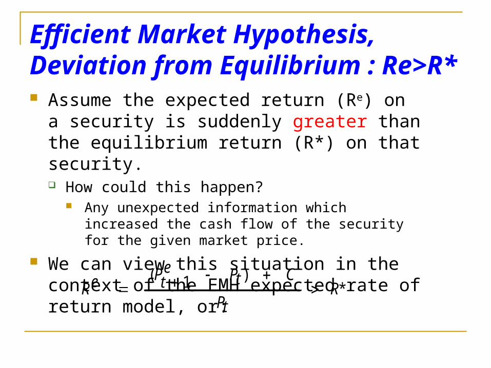
Efficient Market Hypothesis, Deviation from Equilibrium : Re>R* Assume the expected return (Re) on a security

is suddenly greater than the equilibrium return (R*) on that security. How could this happen?

Any unexpected information which increased the cash flow of the security for the given market price.

We can view this situation in the context of the EMH expected rate of return model, or:

*)1(

RtP

CtPetPeR

Restoring Equilibrium

If the expected return (Re) is suddenly greater than the equilibrium return (R*), the current price (Pt) must adjust to satisfy equilibrium, or in this case the current price will rise:

And will do so, until Re = R* As the price rises, the expected return will fall.

e *e If RtPRR

Efficient Market Hypothesis, Deviation from Equilibrium : Re<R* Assume the expected return (Re) on a security

is suddenly less than the equilibrium return (R*) on that security. How could this happen?

Any unexpected information which decreased the cash flow of the security for the given market price.

We can view this situation in the context of the expected rate of return model, or:

*)1(

RtP

CtPetPeR

Restoring Equilibrium

If the expected return (Re) is suddenly less than the equilibrium return (R*), the current price (Pt) must adjust must adjust to satisfy equilibrium, or in this case the current price will fall:

And will do so, until Re = R* As the price falls, the expected return will rise.

e *e If RtPRR

Unexploited Profits According to the EMH, all unexploited profit

opportunities (defined as expected returns greater than equilibrium returns) will be eliminated through price changes. Prices will rise or fall so that expected returns will adjust to

equilibrium return. Conclusion: You can’t beat the market.

When new information affecting the expected return becomes public, prices will adjust.

Unless you have “expected return” information that the rest of the market doesn’t have, you can’t take advantage of this market move.