fMRI Preprocessing

John Ashburner

Contents* Preliminaries

* Rigid-Body and Affine Transformations* Optimisation and Objective Functions* Transformations and Interpolation

* Within Subject: Realignment & Coregistration* Between Subject: Spatial Normalisation & Smoothing

Rigid-Body Transformations* Assume that brain of the same subject doesn’t change

shape or size in the scanner.* Head can move, but remains the same shape and size.* Some exceptions:

* Image distortions.* Brain slops about slightly because of gravity.* Brain growth or atrophy over time.

* If the subject’s head moves, we need to correct the images.* Do this by image registration.

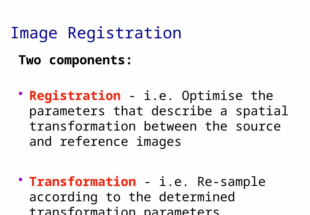
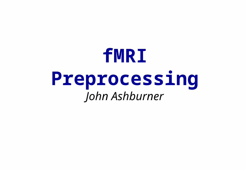
Image Registration

Two components:

• Registration - i.e. Optimise the parameters that describe a spatial transformation between the source and reference images

• Transformation - i.e. Re-sample according to the determined transformation parameters

2D Affine Transforms* Translations by tx and ty

* x1 = x0 + tx

* y1 = y0 + ty

* Rotation around the origin by radians* x1 = cos() x0 + sin() y0

* y1 = -sin() x0 + cos() y0

* Zooms by sx and sy

* x1 = sx x0

* y1 = sy y0

*Shear

* x1 = x0 + h y0

* y1 = y0

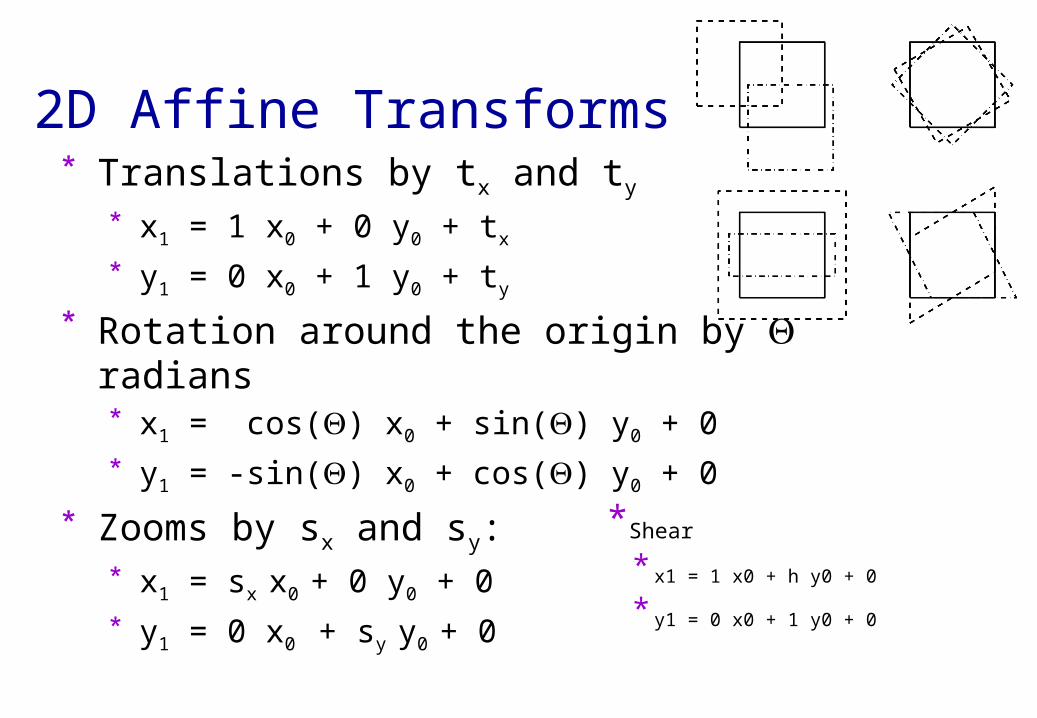
2D Affine Transforms* Translations by tx and ty

* x1 = 1 x0 + 0 y0 + tx

* y1 = 0 x0 + 1 y0 + ty

* Rotation around the origin by radians* x1 = cos() x0 + sin() y0 + 0

* y1 = -sin() x0 + cos() y0 + 0

* Zooms by sx and sy:* x1 = sx x0 + 0 y0 + 0

* y1 = 0 x0 + sy y0 + 0

*Shear

* x1 = 1 x0 + h y0 + 0

* y1 = 0 x0 + 1 y0 + 0

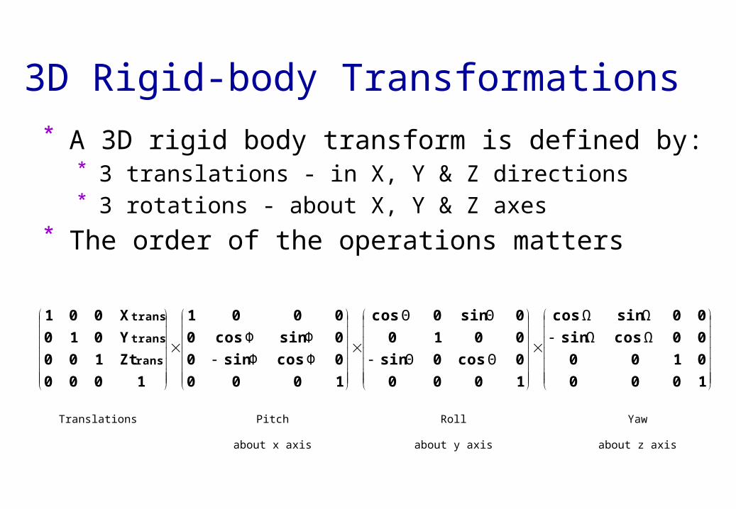
3D Rigid-body Transformations

* A 3D rigid body transform is defined by:* 3 translations - in X, Y & Z directions* 3 rotations - about X, Y & Z axes

* The order of the operations matters

1000

0100

00cossin

00sincos

1000

0cos0sin

0010

0sin0cos

1000

0cossin0

0sincos0

0001

1000

Zt100

Y010

X001

rans

trans

trans

ΩΩ

ΩΩ

ΘΘ

ΘΘ

ΦΦ

ΦΦ

Translations Pitch

about x axis

Roll

about y axis

Yaw

about z axis

Voxel-to-world Transforms* Affine transform associated with each image

* Maps from voxels (x=1..nx, y=1..ny, z=1..nz) to some world co-ordinate system. e.g.,* Scanner co-ordinates - images from DICOM toolbox* T&T/MNI coordinates - spatially normalised

* Registering image B (source) to image A (target) will update B’s voxel-to-world mapping* Mapping from voxels in A to voxels in B is by

* A-to-world using MA, then world-to-B using MB-1

* MB-1 MA

Left- and Right-handed Coordinate Systems

* NIfTI format files are stored in either a left- or right-handed system* Indicated in the header

* Talairach & Tournoux uses a right-handed system* Mapping between them sometimes requires a flip

* Affine transform has a negative determinant

Optimisation

* Image registration is done by optimisation.* Optimisation involves finding some “best”

parameters according to an “objective function”, which is either minimised or maximised

* The “objective function” is often related to a probability based on some model

Value of parameter

Objective function

Most probable solution (global optimum)

Local optimumLocal optimum

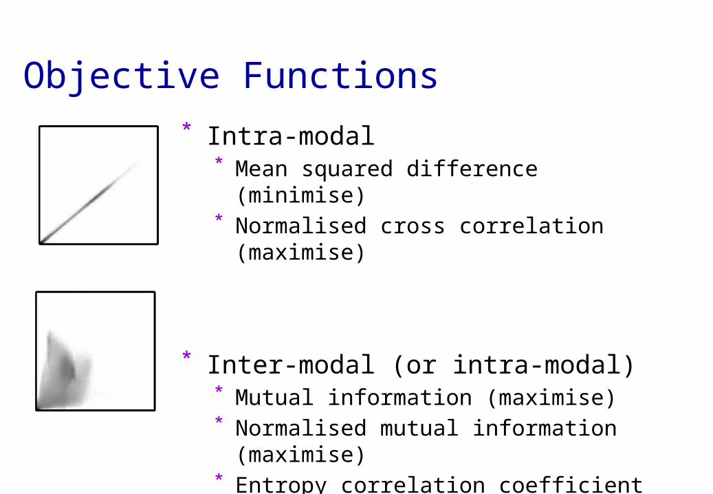
Objective Functions

* Intra-modal* Mean squared difference (minimise)* Normalised cross correlation (maximise)

* Inter-modal (or intra-modal)* Mutual information (maximise)* Normalised mutual information (maximise)* Entropy correlation coefficient (maximise)

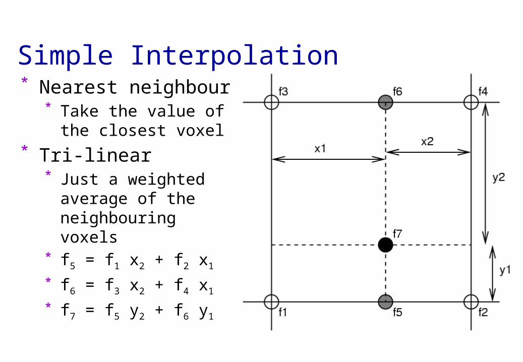
* Nearest neighbour* Take the value of the

closest voxel

* Tri-linear* Just a weighted average

of the neighbouring voxels

* f5 = f1 x2 + f2 x1

* f6 = f3 x2 + f4 x1

* f7 = f5 y2 + f6 y1

Simple Interpolation

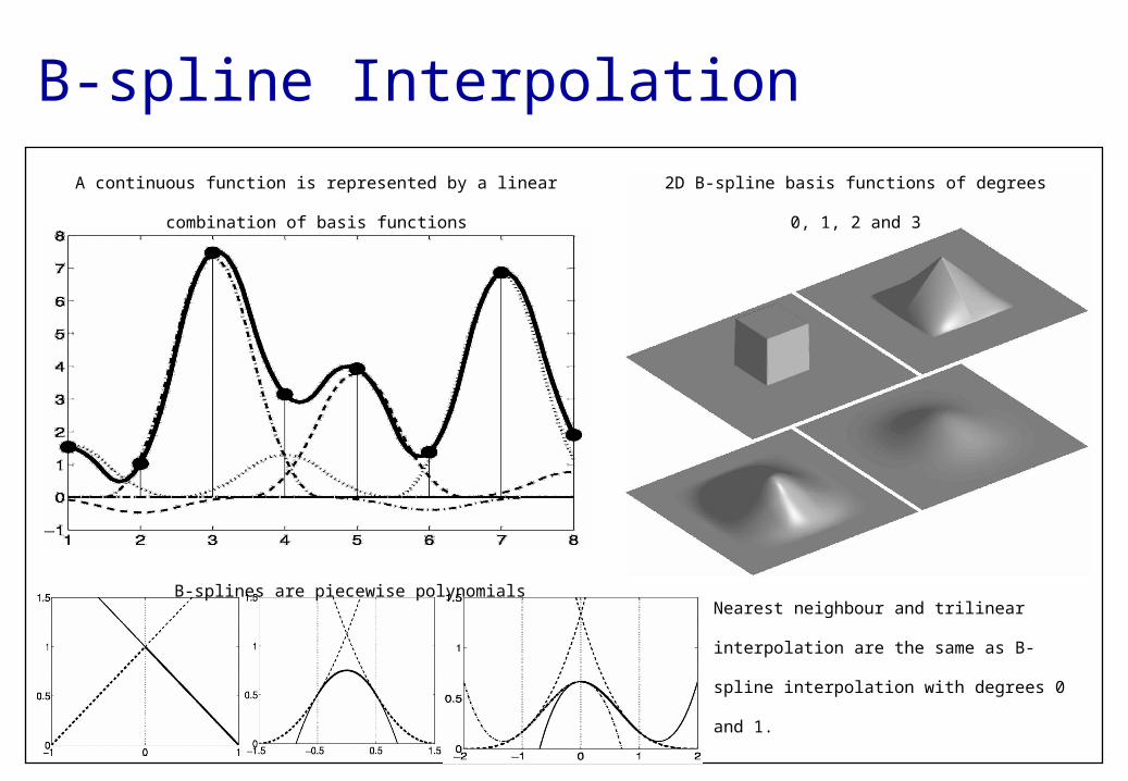
B-spline Interpolation

B-splines are piecewise polynomials

A continuous function is represented by a linear combination of basis

functions

2D B-spline basis functions of degrees 0, 1, 2 and 3

Nearest neighbour and trilinear interpolation are

the same as B-spline interpolation with degrees 0

and 1.

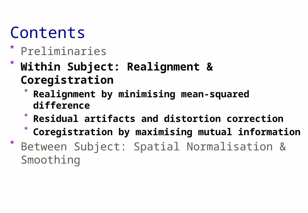
Contents* Preliminaries* Within Subject: Realignment & Coregistration

* Realignment by minimising mean-squared difference* Residual artifacts and distortion correction* Coregistration by maximising mutual information

* Between Subject: Spatial Normalisation & Smoothing

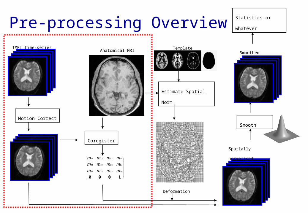
Pre-processing OverviewfMRI time-series

Motion Correct

Anatomical MRI

Coregister

1000

34333231

24232221

14131211

mmmm

mmmm

mmmm

Deformation

Estimate Spatial Norm

Spatially normalised

Smooth

Smoothed

Statistics or

whatever

Template

Mean-squared Difference

* Minimising mean-squared difference works for intra-modal registration (realignment)

* Simple relationship between intensities in one image, versus those in the other* Assumes normally distributed differences

Residual Errors from aligned fMRI

* Re-sampling can introduce interpolation errors* especially tri-linear interpolation

* Gaps between slices can cause aliasing artefacts* Slices are not acquired simultaneously

* rapid movements not accounted for by rigid body model

* Image artefacts may not move according to a rigid body model* image distortion* image dropout* Nyquist ghost

* Functions of the estimated motion parameters can be modelled as confounds in subsequent analyses

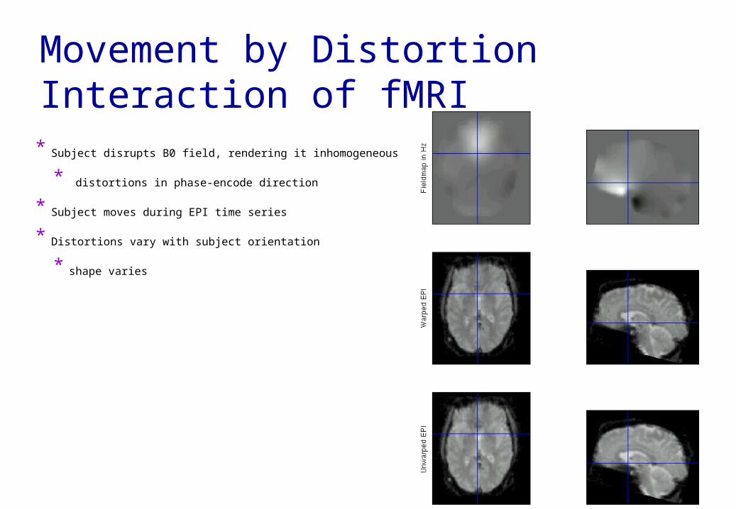
Movement by Distortion Interaction of fMRI* Subject disrupts B0 field, rendering it inhomogeneous

* distortions in phase-encode direction

* Subject moves during EPI time series

* Distortions vary with subject orientation

* shape varies

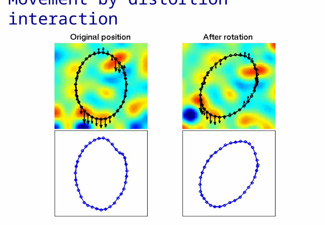
Movement by distortion interaction

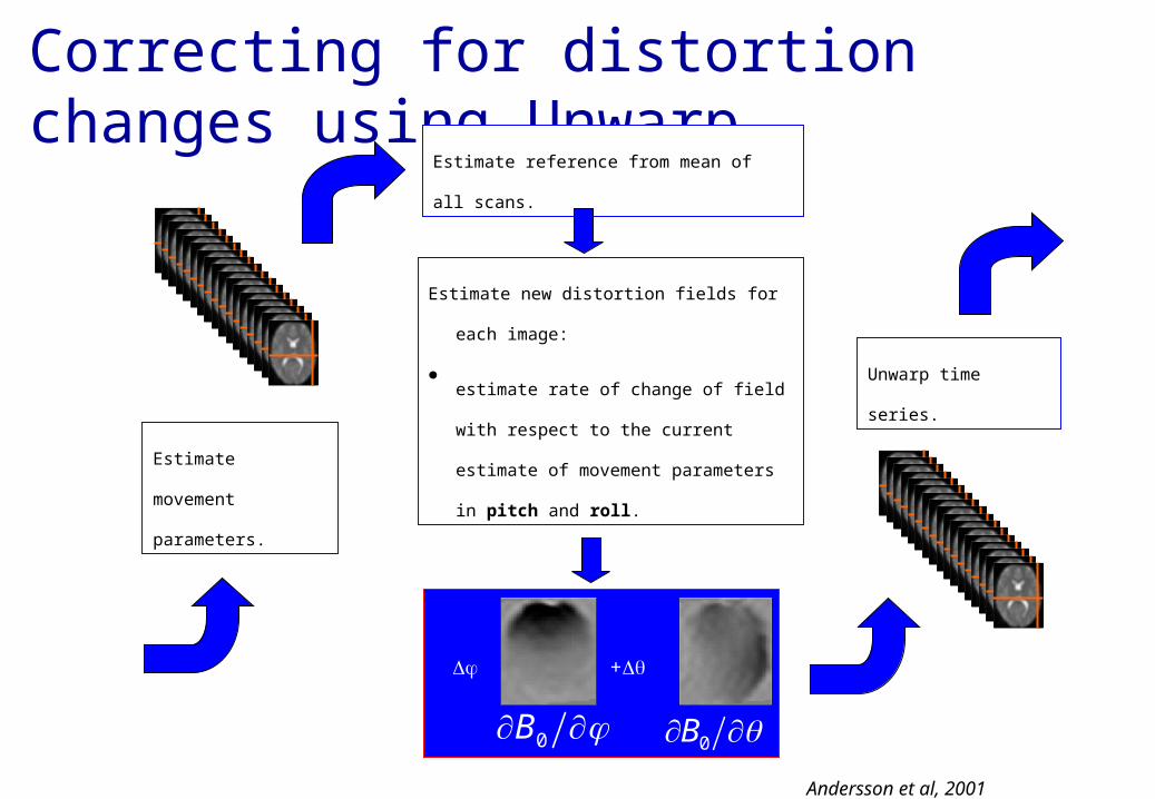
Correcting for distortion changes using Unwarp

Estimate movement

parameters.

Estimate new distortion fields for each image:

•estimate rate of change of field with respect

to the current estimate of movement

parameters in pitch and roll.

Estimate reference from mean of all scans.

Unwarp time series.

0B 0B

+

Andersson et al, 2001

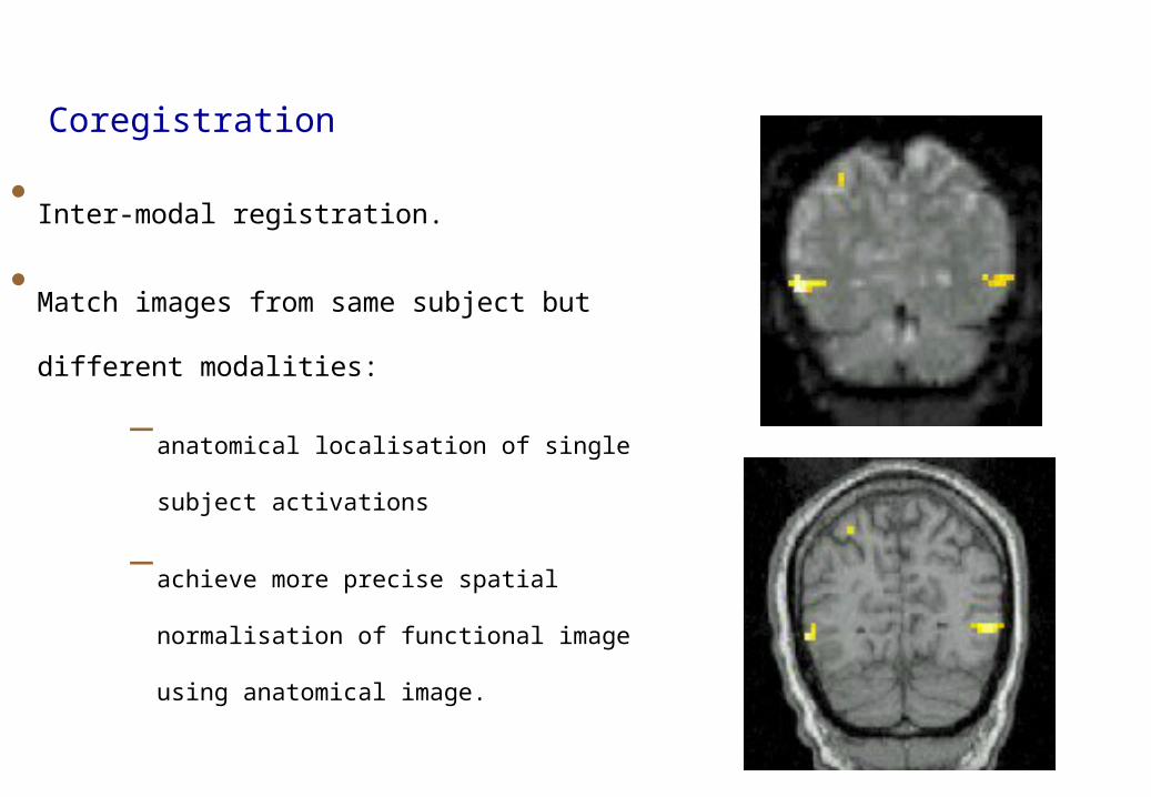
•Inter-modal registration.

•Match images from same subject but different

modalities:

–anatomical localisation of single subject

activations

–achieve more precise spatial normalisation of

functional image using anatomical image.

Coregistration

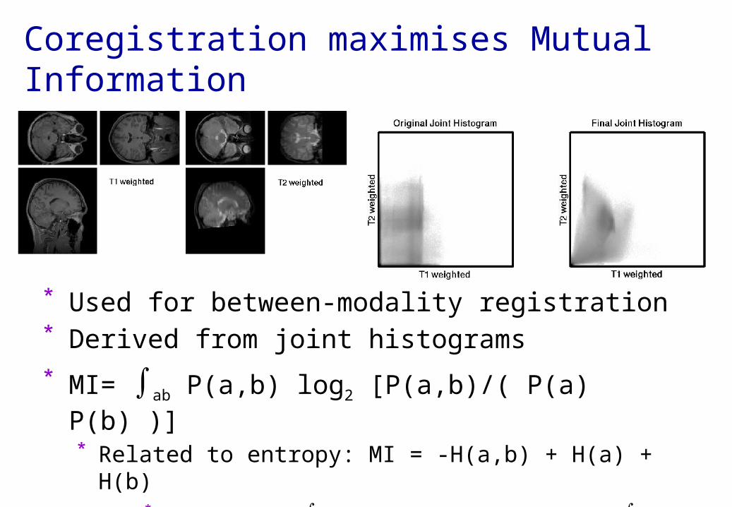
Coregistration maximises Mutual Information

* Used for between-modality registration* Derived from joint histograms

* MI= ab P(a,b) log2 [P(a,b)/( P(a) P(b) )]* Related to entropy: MI = -H(a,b) + H(a) + H(b)

* Where H(a) = -a P(a) log2P(a) and H(a,b) = -a P(a,b) log2P(a,b)

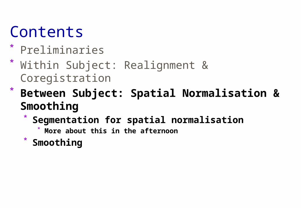
Contents* Preliminaries* Within Subject: Realignment & Coregistration* Between Subject: Spatial Normalisation & Smoothing

* Segmentation for spatial normalisation* More about this in the afternoon

* Smoothing

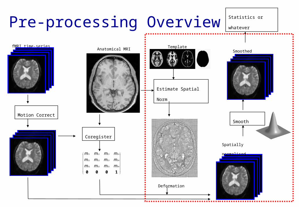
Pre-processing OverviewfMRI time-series

Motion Correct

Anatomical MRI

Coregister

1000

34333231

24232221

14131211

mmmm

mmmm

mmmm

Deformation

Estimate Spatial Norm

Spatially normalised

Smooth

Smoothed

Statistics or

whatever

Template

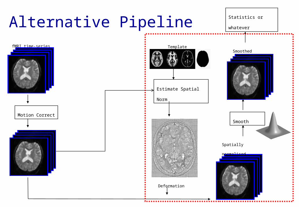
Alternative PipelinefMRI time-series

Motion Correct

Deformation

Estimate Spatial Norm

Spatially normalised

Smooth

Smoothed

Statistics or

whatever

Template

Spatial Normalisation* Brains of different subjects vary in shape and size.* Need to bring them all into a common anatomical space.

* Examine homologous regions across subjects* Improve anatomical specificity* Improve sensitivity

* Report findings in a common anatomical space (eg MNI space)

* In SPM, alignment is achieved by matching grey matter with grey matter and white matter with white matter.* Need to segment.

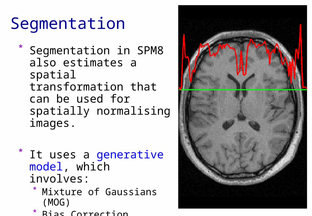
Segmentation

* Segmentation in SPM8 also estimates a spatial transformation that can be used for spatially normalising images.

* It uses a generative model, which involves:* Mixture of Gaussians (MOG)* Bias Correction Component* Warping (Non-linear

Registration) Component

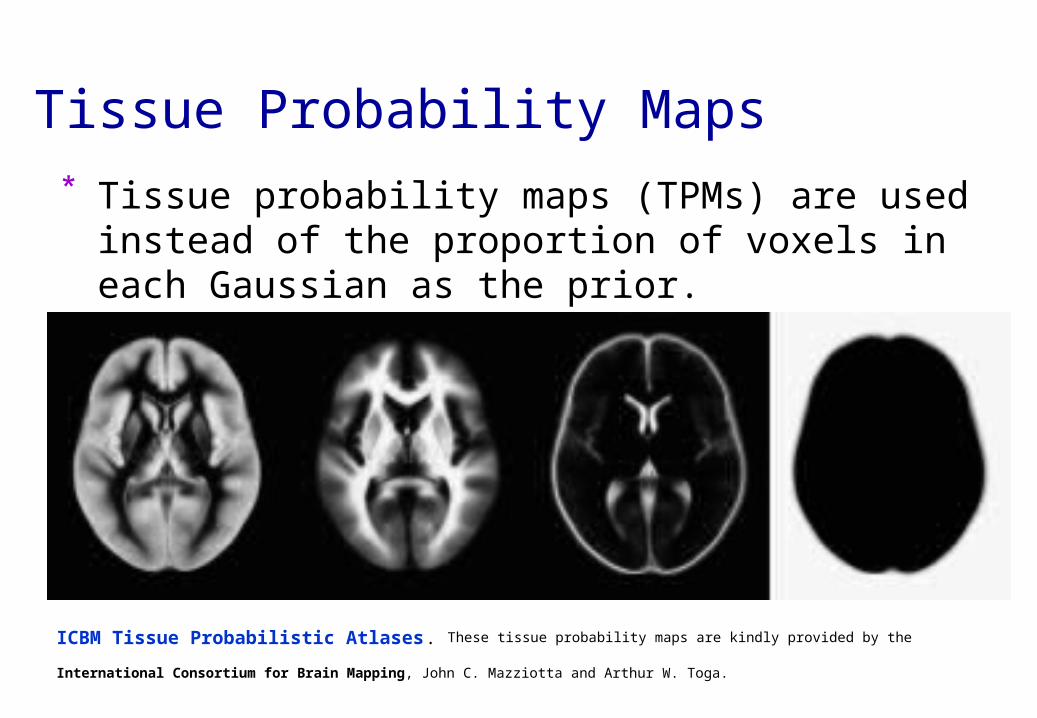
Tissue Probability Maps

* Tissue probability maps (TPMs) are used instead of the proportion of voxels in each Gaussian as the prior.

ICBM Tissue Probabilistic Atlases. These tissue probability maps are kindly provided by the International Consortium for Brain

Mapping, John C. Mazziotta and Arthur W. Toga.

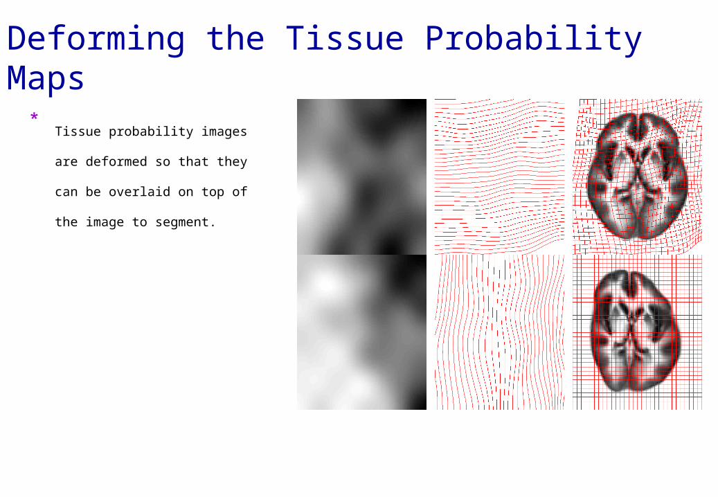
Deforming the Tissue Probability Maps*

Tissue probability images are

deformed so that they can be

overlaid on top of the image to

segment.

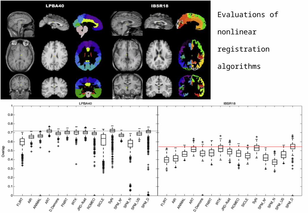
Evaluations of nonlinear

registration algorithms

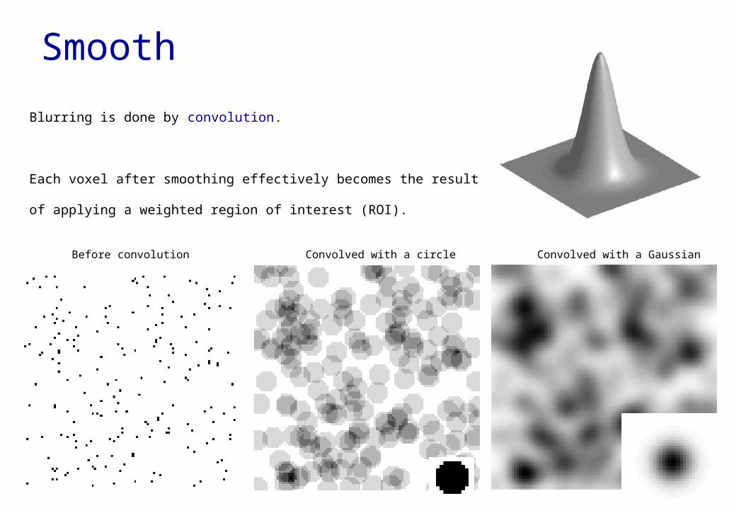
Smooth

Before convolution Convolved with a circle Convolved with a Gaussian

Blurring is done by convolution.

Each voxel after smoothing effectively becomes the result of applying a

weighted region of interest (ROI).

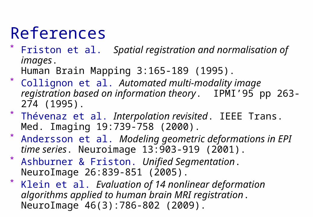
References* Friston et al. Spatial registration and normalisation of images.

Human Brain Mapping 3:165-189 (1995).* Collignon et al. Automated multi-modality image registration

based on information theory. IPMI’95 pp 263-274 (1995).* Thévenaz et al. Interpolation revisited. IEEE Trans. Med. Imaging

19:739-758 (2000).* Andersson et al. Modeling geometric deformations in EPI time

series. Neuroimage 13:903-919 (2001).* Ashburner & Friston. Unified Segmentation. NeuroImage 26:839-

851 (2005).* Klein et al. Evaluation of 14 nonlinear deformation algorithms

applied to human brain MRI registration. NeuroImage 46(3):786-802 (2009).