Submit Manuscript | http://medcraveonline.com

IntroductionIn river basin study, flood routing technique is usually used to

predict the temporal and spatial variations of a flood hydrograph moving through a river reach or reservoir. As the flood wave moves downwards from an upstream point along a river reach, changes in hydrograph shape and timing are due to the routing effects such as storage and flow resistance within the reach. Figure 1 shows the

changes of a flood hydrograph as it moves along a river reach. Routing techniques may be classified broadly into two categories: hydraulic routing, and hydrologic routing. Hydraulic routing techniques are based on the solution of the partial differential equations of unsteady open channel flow, i. e. the St. Venant equations or the dynamic wave equations. Hydrologic routing uses the continuity equation and analytical or empirical relationship between storage in a reach and discharge at the outlet of the channel.

Int Rob Auto J. 2018;4(6):446‒455. 446© 2018 Lang et al. This is an open access article distributed under the terms of the Creative Commons Attribution License, which permits unrestricted use, distribution, and build upon your work non-commercially.

Flood routing for selected gauged basins in Malaysia

Volume 4 Issue 6 - 2018

Hong Jer Lang,¹ Hong Kee An,¹ Hamizah Muhamad²1Monash University, School of Information Technology, Malaysia ²Drainage and Irrigation Department, Malaysia

Correspondence: Hong Jer Lang, Hong and Associates, Monash University, School of Information Technology, Faculty Member, Malaysia, Email Received: September 24, 2018 | Published: December 26, 2018

Abstract

Flood hydrographs are required for the design of hydraulic structures at ungauged locations where no stream flow data are available, as is often the case. In this context, design floods may be derived using a design storm or a regional flood estimation method. However, for specific location in a river where there is a gauging record upstream, it is possible to estimate the flow at the site utilising flood routing techniques. The routing techniques are able to predict the temporal and spatial variations of a flood hydrograph moving through the river reach. Hydrologic routing techniques such as Muskingum and Lag method have been widely used for this purpose. The objective of this paper is to use simple routing techniques to assess the applicability of the methods to two selected Malaysian rivers. Two basins, the Klang river and the Krian river in Peninsular Malaysia were selected for analysis, with river lengths of 0.95 and 7km and gauging records at both upstream and downstream end of the reach. Local inflows from the tributary entering the reach were estimated using synthetic Snyder unit hydrograph method. The performance of the methods was evaluated by comparing the simulated and observed hydrographs graphically and statistically. Best fit parameters for the models were derived using the optimization module of HEC-HMS, and the average parameters obtained were used to validate the routing models using different sets of flood events. Results from optimization and validation runs show that the Muskingum model gives overall better results for both Klang and Krian rivers.

Keywords: flood routing, gauged basins, technique, empirical relationship, hydraulic, boundary conditions

International Robotics & Automation Journal

Research Article Open Access

Figure 1 Discharge hydrograph routing effects.

Flood routing for selected gauged basins in Malaysia 447Copyright:

©2018 Lang et al.

Citation: Lang HJ, An HK, Muhamad H. Flood routing for selected gauged basins in Malaysia. Int Rob Auto J. 2018;4(6):446‒455. DOI: 10.15406/iratj.2018.04.00162

Routing techniques have been widely used in flood forecasting, reservoir and channel design, floodplain studies, and basin simulations. In basin simulation studies, hydrologic routing technique is typically useful in applying to large basin with long river reaches, which are normally subdivided into smaller reaches. An example of using the routing technique is to obtain a flow hydrograph at a point downstream of a location where an observed hydrograph is available. To achieve this, the upstream hydrograph is routed through the reach using a hydrologic routing technique that predicts changes in hydrograph shape and timing. Local flows entering the reach are added to the inflow hydrograph to form the total inflow. Intermediate outflows should be added to the outflow hydrograph so that total volume of inflow is equal to the volume of outflow in the reach. The approach is adequate except there are no significant backwater effects or discontinuities in the water surface because of jumps or bores. If there are downstream controls that affect the routing process through an upstream reach, the channel configuration should be treated as one continuous system. This needs the use of hydraulic routing technique that can incorporate backwater effects as well as internal boundary conditions, such as those associated with culverts, bridges, and weirs.

This paper focused on storage routing, involving solution of the equation of continuity (or conservation of mass), often referred to as storage equation. Storage routing considers the effect of storage on the hydrograph, including translation or delay of the peak, and attenuation or reduction of the hydrograph. The change in magnitude of the hydrograph in respect to the two aspects mentioned depends on the volume of flood relative to the volume of storage through which the flood passes and the physical characteristics of the storage such as length, shape slope and hydraulic resistance of the reach. To this end, storage is the volume of water temporarily stored within the reach at any given time and the water is in transit to the outlet of the downstream end. As storage is temporarily, the total volume of outflow must equal the volume of inflow, and this should be checked in all routing calculations. For the great majority of problems, solutions based on the storage equation are quite satisfactorily.Hydrologic routing techniques

Hydrologic routing used the continuity equation and analytical or empirical relationship between storage and outflow at the downstream end in a river reach . In its simplest form, the continuity equation can be written as inflow minus outflow equals the rate of change of storage within the reach:

SI O

t∆

− =∆

(1)

where

I=The average inflow to the reach during

O=The average outflow from the reach during

S=Storage within the reach

t∆ =computation interval

Hydrologic routing techniques have been widely applied to solve river routing problems, for example, Ansari and Ukarnde,1 Song and Kong,2 Kumar and Raju,3 Elbashir,4 Reggiani et al,5 Sujikumar and Suman,6 Tewolde and Smithers.7

In this paper, calculation of river routing for Klang and Krian rivers is based on the inflow and outflow of observed floods adjusted to equal volumes within the selected period of analysis. Two commonly used hydrologic routing methods are adopted for analysis, namely

the Muskingum and the lag methods. Recorded flood hydrographs of two gauging stations of Klang river (within a distance of 0.95 km ) and Krian river (within a distance of 7km), i were used to estimate the model parameters of the two routing methods chosen using the optimization module of the HEC-HMS program.8

Materials and methodsThe following sections present the details of floods chosen for

analysis and the methods used in river routing for the Klang and Krian rivers.

Klang and krian rivers

Klang basin is located in the central part of west Peninsular Malaysia. The basin is hilly in the lower portion and the upper basin is mountainous rising to a height of 1430 m. The maximum length and breadth of the basin are 29 km and 27 km respectively. Hilly areas are under palm oil and small low-lying area is under tin mining. The other area is urban and mined lands. Krian River is located in north western Peninsular Malaysia. The basin has length and breadth of 31 and 23km respectively. About 50% of the basin is occupied by steep mountainous country rising to 1500 m while the remaining is undulating to flat lands. Oil palm plantations cover the low-lying area while the hills are covered with forest. The hills are extremely steep.The locations of the two basins are shown in Figure 2.

Figure 2 Klang and krian rivers.

Flood hydrographs of klang and krian rivers

Klang river has been gauged at several locations (Figure 3). The gauging stations at Leboh Pasar Kuala Lumpur and Sulaiman Bridge in the centre of Kuala Lumpur city are within a distance of 950m. Concurrent discharge data are available from the automatic recorders from these stations from October 1973 to December 1974. Details of the gauging stations and records available are shown in Table 1. Examination of the flow records shows that several flood events in this period are available and can be adopted for river routing analysis. Selected flood events used in this study are shown in Table 2. As the area between the gauging stations is small and no tributaries enter the reach between the stations, the runoff volume of inflow hydrograph should equal to that of outflow hydrograph. Therefore, within the analysis period, if the outflow runoff volume is found to be lower than the inflow volume, the outflow hydrograph was scaled proportionally so that the volume of flow at upstream side is equal to that of downstream as there are no records available for local inflow. The start and end times for the analysis are selected so that average discharges in the reach were approximately equal in the start and end time of the hydrographs. Figure 4 and Figure 5 show two of the selected flood hydrographs recorded at the gauging stations.

Flood routing for selected gauged basins in Malaysia 448Copyright:

©2018 Lang et al.

Citation: Lang HJ, An HK, Muhamad H. Flood routing for selected gauged basins in Malaysia. Int Rob Auto J. 2018;4(6):446‒455. DOI: 10.15406/iratj.2018.04.00162

Figure 3 Gauging stations of klang river.

Legend:

Gauging

Stations

Sg Klang

River Basin

Table 1 Details of the gauging records, klang basin

Station ID Station name Period of record Catchment area (km²)

3116432 Klang at Leboh Pasar Kuala Lumpur Jul 1960-Dec 1974 464

3116430 Klang at Sulaiman Bridge Oct 1973-to date 468

Table 2 Selected floods used for routing analysis, klang basin

Flood event Period Peak Flow (m³/s)

At Leboh Pasar At Sulaiman Bridge

1 06/12/1973 18:00 to 11/12/1973 10:00 191.2 151.3

2 22/12/1973 10:00 to 24/12/1973 20:30 75.5 75.7

3 24/11/1973 13:00 to 27/11/1973 16:00 110.9 93.6

4 02/05/1974 15:00 to 03/05/1974 19:00 63.5 63.8

5 07/12/1974 12:00 to 10/12/1974 04:00 56.4 53.9

6 10/12/1974 10:00 to 13/12/1974 07:00 69.3 70.8

Figure 4 Flood hydrographs of 24/11/1973 (s for sulaiman bridge, lp for leboh pasar).

Figure 5 Flood hydrographs of 07/12/1974 (s for Sulaiman Bridge, lp for Leboh Pasar).

Flood routing for selected gauged basins in Malaysia 449Copyright:

©2018 Lang et al.

Citation: Lang HJ, An HK, Muhamad H. Flood routing for selected gauged basins in Malaysia. Int Rob Auto J. 2018;4(6):446‒455. DOI: 10.15406/iratj.2018.04.00162

The gauging stations of Krian are shown in Figure 6. The gauging stations at Selama Dusun Rimau are within a distance of 7 km. Concurrent discharge data are available from the automatic recorders from these stations from April 1973 to December 1973. Details of the

gauging stations and records available are shown in Table 3. Selected flood events from the records available used in this study are shown in Table 4.

Figure 6 Gauging stations of krian basin.

Table 3 Details of the gauging records krian basin

Station ID Station name Period of record Catchment area (km²)

5206432 Krian at Selama Jul 1960–to date 629

5106431 Krian At Dusun Rimau Jul1960-Nov 1974 694

Table 4 Selected floods used for routing analysis, krian basin

Flood Event Period Peak flow (m³/s)

At selama At dusun rimau

1 23/10/1973 15:00 to 09/11/1973 20:00 151 120.9

2 31/07/1973 15:00 to 08/08/1973 23:00 136.7 109.3

3 12/09/1973 22:00 to 17/09/1973 19:00 98.2 87.8

4 02/10/1973 11:00 to 10/10/1973 22:00 70.7 66.2

As there is an ungauged tributary, Terap river entering the reach between the stations, the total inflow into the reach includes flows from Selama gauging station and the ungauged Terap tributary. As stated in Linsley et al(1980) the inflow hydrograph from the tributary can be estimated using synthetic unit hydrograph. For this study, the flood hydrographs of the Terap river for the flood events listed in Table 4 were estimated using Hydrological Procedure No 11.9 Hydrological Procedure No 11 used Snyder Unit Hydrograph method to estimate lag time and peaking coefficients for ungauged basins. The formula used to estimate lag time is:

0.4143 0.1403 0.43210.639p

t A L S −= (2)

Where A is the basin area in km²

L is the length of basin main stream from basin divide to basin outlet

S is the weighted slope of the main stream

And a peaking coefficient of 0.55 was adopted

For Terap A=65

L=18

And S=1.67%

And the lag time calculated is 4.33hours

Base flow of Terap river used to compute the flood hydrograph of each event is assumed to be proportional to those of Selama and Dusun Rimau. Rainfall records from an autographic station near to the Terap river are used for estimating floods using the Snyder unit hydrograph method. Within the analysis period, if the outflow runoff volume is found to be lower than the inflow volume, the outflow hydrograph was scaled proportionally so that the volume of flow at upstream side is equal to the flow volume at the downstream end.

Flood routing for selected gauged basins in Malaysia 450Copyright:

©2018 Lang et al.

Citation: Lang HJ, An HK, Muhamad H. Flood routing for selected gauged basins in Malaysia. Int Rob Auto J. 2018;4(6):446‒455. DOI: 10.15406/iratj.2018.04.00162

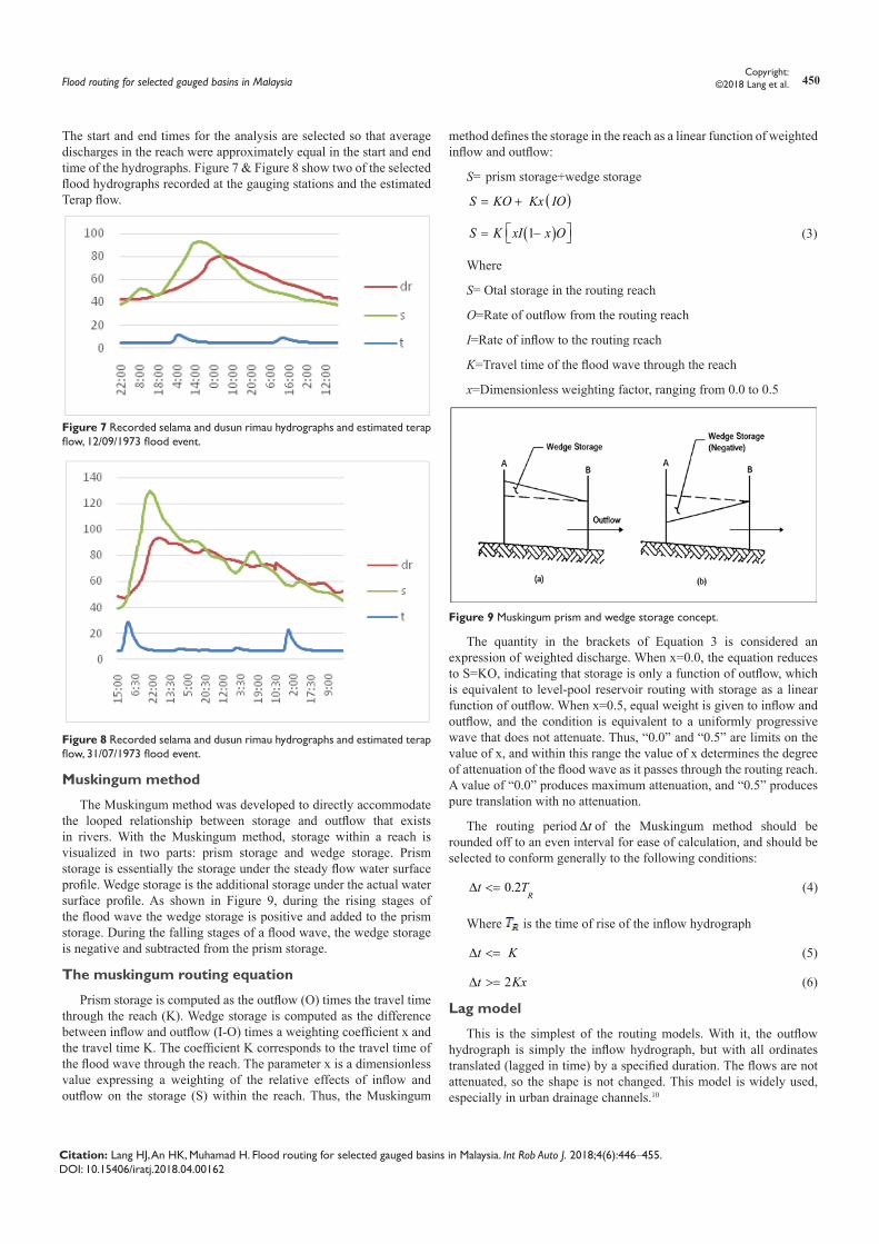
The start and end times for the analysis are selected so that average discharges in the reach were approximately equal in the start and end time of the hydrographs. Figure 7 & Figure 8 show two of the selected flood hydrographs recorded at the gauging stations and the estimated Terap flow.

Figure 7 Recorded selama and dusun rimau hydrographs and estimated terap flow, 12/09/1973 flood event.

Figure 8 Recorded selama and dusun rimau hydrographs and estimated terap flow, 31/07/1973 flood event.

Muskingum method

The Muskingum method was developed to directly accommodate the looped relationship between storage and outflow that exists in rivers. With the Muskingum method, storage within a reach is visualized in two parts: prism storage and wedge storage. Prism storage is essentially the storage under the steady flow water surface profile. Wedge storage is the additional storage under the actual water surface profile. As shown in Figure 9, during the rising stages of the flood wave the wedge storage is positive and added to the prism storage. During the falling stages of a flood wave, the wedge storage is negative and subtracted from the prism storage.

The muskingum routing equation

Prism storage is computed as the outflow (O) times the travel time through the reach (K). Wedge storage is computed as the difference between inflow and outflow (I-O) times a weighting coefficient x and the travel time K. The coefficient K corresponds to the travel time of the flood wave through the reach. The parameter x is a dimensionless value expressing a weighting of the relative effects of inflow and outflow on the storage (S) within the reach. Thus, the Muskingum

method defines the storage in the reach as a linear function of weighted inflow and outflow:

S= prism storage+wedge storage

( ) S KO Kx IO= +

( )1 S K xI x O= − (3)

Where

S= Otal storage in the routing reach

O=Rate of outflow from the routing reach

I=Rate of inflow to the routing reach

K=Travel time of the flood wave through the reach

x=Dimensionless weighting factor, ranging from 0.0 to 0.5

Figure 9 Muskingum prism and wedge storage concept.

The quantity in the brackets of Equation 3 is considered an expression of weighted discharge. When x=0.0, the equation reduces to S=KO, indicating that storage is only a function of outflow, which is equivalent to level-pool reservoir routing with storage as a linear function of outflow. When x=0.5, equal weight is given to inflow and outflow, and the condition is equivalent to a uniformly progressive wave that does not attenuate. Thus, “0.0” and “0.5” are limits on the value of x, and within this range the value of x determines the degree of attenuation of the flood wave as it passes through the routing reach. A value of “0.0” produces maximum attenuation, and “0.5” produces pure translation with no attenuation.

The routing period t∆ of the Muskingum method should be rounded off to an even interval for ease of calculation, and should be selected to conform generally to the following conditions:

0.2R

t T∆ <= (4)

Where is the time of rise of the inflow hydrograph

t K∆ <= (5)

2 t Kx∆ >= (6)

Lag model

This is the simplest of the routing models. With it, the outflow hydrograph is simply the inflow hydrograph, but with all ordinates translated (lagged in time) by a specified duration. The flows are not attenuated, so the shape is not changed. This model is widely used, especially in urban drainage channels.10

Flood routing for selected gauged basins in Malaysia 451Copyright:

©2018 Lang et al.

Citation: Lang HJ, An HK, Muhamad H. Flood routing for selected gauged basins in Malaysia. Int Rob Auto J. 2018;4(6):446‒455. DOI: 10.15406/iratj.2018.04.00162

Mathematically, the downstream ordinates are computed by:

{ O It t= t<lag

tI lag− t>=lag

where

Ot=outflow hydrograph ordinate at time

t

I =inflow hydrograph ordinate at time t; and

Lag=time by which the inflow ordinates are to be lagged.

Figure 10 illustrates the results of application of the lag model. In the figure, the upstream (inflow) hydrograph is the boundary condition. The downstream hydrograph is the computed outflow, with each ordinate equal to an earlier inflow ordinate, but lagged in time. The lag model is a special case of other models, as its results can be duplicated if parameters of those other models are carefully chosen. For example, if X=0.50 and K t= ∆ in the Muskingum model, the computed outflow hydrograph will equal the inflow hydrograph lagged by K.11

Figure 10 Lag model examples.

Estimating the lag

If observed flow hydrographs are available, the lag can be estimated from these as the elapsed time between the time of the centroid of areas of the two hydrographs, between the times of hydrograph peaks, or between the times of the midpoints of the rising limbs.

Calibration of routing models using HEC-HMS

The river routing models consist of parameters that must be specified in order to use the model for estimating runoff or routing hydrographs. For the routing models, appropriate values for the parameters can be selected if stream flow observations are available, by model calibration. Calibration uses observed hydro meteorological data in a systematic search for parameters that yield the best fit of the computed results to the observed runoff. This search is often referred to as optimization. In this Paper, HEC-HMS of Hydrologic Engineering Centre8 is adopted for this purpose.

Calibration procedure

In HEC-HMS, the systematic search for the best (optimal) parameter values begins with data collection. For routing models, observations of both inflow to and outflow from the routing reach are required. Table 5 offers some guide lines for collecting these data.

The next step is to select initial estimates of the parameters. As with any search, the better these initial estimates (the starting point of the search), the quicker the search will yield a solution. Given these

initial estimates of the parameters, the models can be used with the observed boundary conditions (upstream flow) to compute the output, the channel outflow hydrograph.

Table 5 Guide lines for collecting data for routing model calibration

The upstream and downstream hydrograph time series must represent flow for the same period of time.

The volume of the upstream hydrograph should approximately equal the volume of the downstream hydrograph, with minimum lateral inflow. The lumped routing models in HEC-HMS assume that these volumes are equal.

The duration of the downstream hydrograph should be sufficiently long so that the total volume represented equals the volume of the upstream hydrograph.

At this point, the program compares the computed hydrograph to the observed hydrograph. The goal of this comparison is to judge how well the model “fits” the real hydrologic system. If the fit is not satisfactory, the program systematically adjusts the parameters and reiterates. When the fit is satisfactory, the program will report the optimal parameter values. The presumption is that these parameter values then can be used routing computations that are the goal of the flood runoff analyses.

Goodness-of-fit indices

To compare a computed hydrograph to an observed hydrograph, HEC-HMS computes indices of the goodness-of-fit. The three indices calculated are:

a) Mean absolute error (MAE)

b) Root mean square error (RMSE)

c) Nash –Sutcliffe efficiency coefficient (NSE)

Where

1n

si oiQ QMAE

n−∑

= (8)

21 ( )n

si oiQ QRMSE

n−∑= (9)

21

2

( )1

( )

nsi oi

oi Q

Q QNAE

Q

−∑= −

− (10)

Where

Qoi is the ith observed flow and

Qsi is the ith simulated flow Q is the average of the observed flow

n is the number of data points

The best fit between the calculated and observed hydrographs using these parameters occurs when NAE approaches 1, RMSE and MAE approach 0. A lower MAE and RMSE will give a better fit and a better model performance, on the other hand, a higher NAE gives a better fit for the model (NAE is normally between 0 and 1)ResultsResults from calibration runs

a. Of the six flood events chosen for this Study for Klang river, 3 are used for calibrating the routing models and the rest used

Flood routing for selected gauged basins in Malaysia 452Copyright:

©2018 Lang et al.

Citation: Lang HJ, An HK, Muhamad H. Flood routing for selected gauged basins in Malaysia. Int Rob Auto J. 2018;4(6):446‒455. DOI: 10.15406/iratj.2018.04.00162

for model validation. And for Krian 3 are used for calibration and one for validation. Calibration results for Klang and Krian rivers using Muskingum method are presented in Table 6 and Table 7.

b. Figure 11 and Figure 12 show the observed and predicted hydrographs for the 02/05/1974 floods for Klang river and 06/12/1973 floods for Krian river using Muskingam model.

Calibration results using Lag method for Klang and Krian rivers are presented in Table 8 & Table 9.

c. Figure 13 & Figure 14 show the observed and predicted hydrographs for the 02/05/1974 and 09/12/1973 floods using Lag model respectively for Klang and Krian. Results show that the Muskingum method gives a better fit as it has overall better goodness of fit indices.

Table 6 Calibration results for muskingum method, klang river

Flood occurred on K, hours No of subreaches x Peak flow (m3/s) MAE RMSE NAE

Qo Qs

2/5/1974 0.8 1 0.142 63.8 62.7 1.1 1.3 0.992

7/12/1974 0.61 1 0.141 55.6 53.9 1.3 2.5 0.938

6/12/1973 0.61 1 0.142 151.3 189.5 5.7 9.2 0.935

Average 0.68 1 0.142

Table 7 Calibration results for muskingum method, krian river

Flood occurred on K, hours No of subreaches x Peak flow (m3/s) MAE RMSE NAE

Qo Qs

12/9/1973 15.4 1 0.108 87.8 86.2 1.4 1.9 0.977

31/07/1973 17 1 0.108 109.3 112.9 3.1 3.9 0.932

23/10/1973 19 1 0.108 120.9 133.4 4.7 6.4 0.832

Average 17 1 0.108

Table 8 Calibration results for lag method, klang river

Flood occurred on Lag (minutes) Peak flow (m3/s) MAE RMSE NAE

Qo Qs

2/5/1974 48 63.5 63.8 1.1 1.6 0.987

7/12/1974 123 56.3 53.9 2.9 5.8 0.664

6/12/1973 24.5 151.1 191.1 5.7 9.1 0.935

Average 65

Table 9 Calibration results for lag method, krian river

Flood occurred on Lag (minutes) Peak flow (m3/s) MAE RMSE NAE

Qo Qs

27007 784 87.8 98.2 4.8 5.9 0.775

31/07/1973 697 109.3 136.6 6.1 8.5 0.673

23/10/1973 24.5 120.9 150.9 7.4 9.8 0.603

Average 65

Flood routing for selected gauged basins in Malaysia 453Copyright:

©2018 Lang et al.

Citation: Lang HJ, An HK, Muhamad H. Flood routing for selected gauged basins in Malaysia. Int Rob Auto J. 2018;4(6):446‒455. DOI: 10.15406/iratj.2018.04.00162

Figure 11 Observed & predicted outflow hydrographs of the 02/05/1974 floods (muskingum model), klan river.

Figure 12 Observed inflow and outflow and predicted outflow hydrographs of the 12/09/1973 floods (muskingum model), krian river.

Results from validation runs

a. The average calibrated parameters of the routing models were used to predict the outflow hydrographs for 3 recorded floods in Klang basin and one flood for Krian basin using Muskingum and Lag methods. Results of Muskingum method are shown in Table 10 & Table 11.

b. Figure 15 & Figure 16 show the observed and predicted

hydrographs for the 10/12/1973 and 02/10/1973 floods using Muskingam model for Klang and Krian respectively.

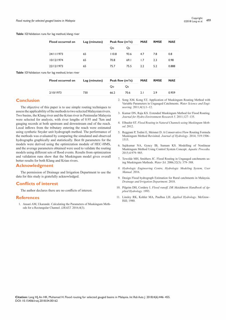
c. The Lag model validation results are shown in Table 12 &Table 13.

d. Figure 17 & Figure 18 show the observed and predicted hydrographs for the 10/12/1974 and 02/10/1973 floods using Lag model for Klang and Krian rivers respectively.

e. Results show that the Muskingum method gives better predicted hydrographs as it has overall better goodness of fit indices obtained from the validation runs.

Figure 13 Observed and predicted outflow hydrographs of the 02/05/1974 floods (lag model), klang river.

Figure 14 Observed inflow and outflow and predicted outflow hydrographs of the 12/09/1973 floods (lag model), krian river.

Flood routing for selected gauged basins in Malaysia 454Copyright:

©2018 Lang et al.

Citation: Lang HJ, An HK, Muhamad H. Flood routing for selected gauged basins in Malaysia. Int Rob Auto J. 2018;4(6):446‒455. DOI: 10.15406/iratj.2018.04.00162

Table 10 Validation runs for muskingum method, klang river

Flood occurred on K , hours No of subreaches x Peak flow (m3/s) MAE RMSE NAE

Qo Qs

24/11/1973 0.68 1 0.142 109. 8 93.6 4.1 6.5 0.861

10/12/1974 0.68 1 0.142 70.8 68.4 2.2 3.4 0.957

22/12/1973 0.68 1 0.142 75.7 75.1 1.5 3.6 0.945

Table 11 Validation runs for muskingum method, krian river

Flood occurred on K, hours No of subreaches x Peak flow (m3/s) MAE RMSE NAE

Qo Qs

2/10/1973 17 1 0.11 66.2 62.5 2.1 2.5 0.969

Figure 15 Observed & predicted outflow hydrographs of the 10/12/1974 floods (muskingum model), klang river.

Figure 16 Observed & predicted outflow hydrographs of the 02/10/1973 floods (muskingum model), krian river.

Figure 17 Observed and predicted outflow hydrographs of the 10/12/1974 floods (lag model), klang river.

Figure 18 Observed and predicted outflow hydrographs of the 02/10/1973 floods (lag model), krian river.

Flood routing for selected gauged basins in Malaysia 455Copyright:

©2018 Lang et al.

Citation: Lang HJ, An HK, Muhamad H. Flood routing for selected gauged basins in Malaysia. Int Rob Auto J. 2018;4(6):446‒455. DOI: 10.15406/iratj.2018.04.00162

Table 12 Validation runs for lag method, klang river

Flood occurred on Lag (minutes) Peak flow (m3/s) MAE RMSE NAE

Qo Qs

24/11/1973 65 110.8 93.6 4.7 7.8 0.8

10/12/1974 65 70.8 69.1 1.7 2.3 0.98

22/12/1973 65 75.7 75.5 2.2 5.2 0.888

Table 13 Validation runs for lag method, krian river

Flood occurred on Lag (minutes) Peak flow (m3/s) MAE RMSE NAE

Qo Qs

2/10/1973 730 66.2 70.6 2.1 2.9 0.959

ConclusionThe objective of this paper is to use simple routing techniques to

assess the applicability of the methods to two selected Malaysian rivers. Two basins, the Klang river and the Krian river in Peninsular Malaysia were selected for analysis, with river lengths of 0.95 and 7km and gauging records at both upstream and downstream end of the reach. Local inflows from the tributary entering the reach were estimated using synthetic Snyder unit hydrograph method. The performance of the methods was evaluated by comparing the simulated and observed hydrographs graphically and statistically. Best fit parameters for the models were derived using the optimization module of HEC-HMS, and the average parameters obtained were used to validate the routing models using different sets of flood events. Results from optimization and validation runs show that the Muskingum model gives overall better results for both Klang and Krian rivers.Acknowledgment

The permission of Drainage and Irrigation Department to use the data for this study is gratefully acknowledged.

Conflicts of interestThe author declares there are no conflicts of interest.

References1. Ansari AM, Ukarande. Calculating the Parameters of Muskingum Meth-

ods for a Rectangular Channel. IJRAET. 2016;4(3).

2. Song XM, Kong FZ. Application of Muskingum Routing Method with Variable Parameters in Ungauged Catchments. Water Science and Engi-neering. 2011;4(1):1–12.

3. Kumar DN, Raju KS. Extended Muskingum Method for Flood Routing. Journal for Hydro-Environment Research 5. 2011;127–135.

4. Elbashir ST. Flood Routing in Natural Channels using Muskingum Meth-od. 2012.

5. Reggiani P, Todini E, Meisner D. A Conservative Flow Routing Formula Muskingum Method Revisited. Journal of Hydrology. 2014; 519:1506–1515.

6. Sajikumar NA, Gyncy IB, Sumam KS. Modelling of Nonlinear Muskingum Method Using Control System Concept. Aquatic Procedia. 2015;4:979–985.

7. Tewolde MH, Smithers JC. Flood Routing in Ungauged catchments us-ing Muskingum Methods. Water SA. 2006;32(3): 379–388.

8. Hydrologic Engineering Centre, Hydrologic Modeling System, User Manual. 2016.

9. Design Flood hydrograph Estimation for Rural catchments in Malaysia. Drainage and Irrigation Department. 2018.

10. Pilgrim DH, Cordery I. Flood runoff, DR Maiddment Handbook of Ap-plied Hydrology. 1993.

11. Linsley RK, Kohler MA, Paulhus LH. Applied Hydrology. McGraw–Hill; 1980.