Fisheye camera system calibration for automotive … · Fisheye Camera System Calibration for Automotive ... List of Figures ... extrinsic and intrinsic calibration are part of the

Masterarbeit am Institut für Informatik der Freien Universität Berlin,

Dahlem Center for Machine Learning and Robotics

Fisheye Camera System Calibration for Automotive

Applications

Christian Kühling

Matrikelnummer: 4481432

[email protected]

Erstgutachter: Prof. Dr. Daniel Göhring

Zweitgutachter: Prof. Dr. Raúl Rojas

Betreuer: Fritz Ulbrich

Berlin, 05.05.2017

mailto:[email protected]

Abstract

In this thesis, the imagery of the fisheye camera system mounted to the au-tonomous car MadeInGermany of the Freie Universität Berlin is processedand calibrated. Hereby, distortions caused by fisheye lenses are automati-cally corrected and a surround view of the vehicle is created.Over the next decade, autonomous cars are expected to radically changemobility as we know it. While intelligent software systems made astonishingimprovements over the past years, the eventual quality of autonomous carsdepends on their sensors capturing the environment.One of the most important sensors are cameras for visual input. Hence, itdoes not surprise that current autonomous prototypes often have multiplecameras, for example to prevent having blind spots. For this specific reason,fisheye lenses with a large field of views are often used.To utilize recordings of these camera systems by computer vision algorithms,a camera calibration is required. It consists of the intrinsic calibration,rectifying possible distortions and extrinsic calibration, determining positionand pose of the cameras.

Statement of Academic Integrity

Hereby, I declare that I have composed the presented paper independentlyon my own and without any other resources than the ones indicated. Allthoughts taken directly or indirectly from external sources are properly de-noted as such. This paper has neither been previously submitted to anotherauthority nor has it been published yet.

05.05.2017

Christian Kühling

Contents

1 Introduction 1

1.1 Motivation . . . . . . . . . . . . . . . . . . . . . . . . . . . . 11.2 AutoNOMOS project . . . . . . . . . . . . . . . . . . . . . . . 21.3 Goal . . . . . . . . . . . . . . . . . . . . . . . . . . . . . . . . 31.4 Thesis structure . . . . . . . . . . . . . . . . . . . . . . . . . . 41.5 Related Work . . . . . . . . . . . . . . . . . . . . . . . . . . . 4

2 Fundamentals 5

2.1 Hardware setup . . . . . . . . . . . . . . . . . . . . . . . . . . 52.2 Theoretical fundamentals . . . . . . . . . . . . . . . . . . . . 8

2.2.1 Mathematical notations . . . . . . . . . . . . . . . . . 82.2.2 Coordinate systems . . . . . . . . . . . . . . . . . . . 92.2.3 Pinhole camera model . . . . . . . . . . . . . . . . . . 10

2.3 Intrinsic camera calibration . . . . . . . . . . . . . . . . . . . 142.3.1 Mei’s calibration toolbox . . . . . . . . . . . . . . . . 142.3.2 Scaramuzza’s OcamCalibToolbox . . . . . . . . . . . . 162.3.3 OpenCV camera calibration . . . . . . . . . . . . . . . 18

2.4 Extrinsic camera calibration . . . . . . . . . . . . . . . . . . . 212.4.1 Approaches . . . . . . . . . . . . . . . . . . . . . . . . 212.4.2 CamOdoCal . . . . . . . . . . . . . . . . . . . . . . . . 25

2.5 Used libraries and software . . . . . . . . . . . . . . . . . . . 322.5.1 ROS . . . . . . . . . . . . . . . . . . . . . . . . . . . . 322.5.2 OpenCV . . . . . . . . . . . . . . . . . . . . . . . . . . 322.5.3 LibPCAP . . . . . . . . . . . . . . . . . . . . . . . . . 322.5.4 LibJPEG-turbo . . . . . . . . . . . . . . . . . . . . . . 332.5.5 Docker . . . . . . . . . . . . . . . . . . . . . . . . . . . 332.5.6 MATLAB . . . . . . . . . . . . . . . . . . . . . . . . . 33

3 Implementation 35

3.1 The camera driver . . . . . . . . . . . . . . . . . . . . . . . . 353.2 Decompression of received compressed JPEG images . . . . . 363.3 Extrinsic and intrinsic camera calibration script . . . . . . . . 373.4 Rectification of distorted fisheye images . . . . . . . . . . . . 42

ii

3.5 Surround view of the MIG . . . . . . . . . . . . . . . . . . . . 423.6 Overview of the Implementation . . . . . . . . . . . . . . . . 45

4 Results and conclusion 47

4.1 Results and discussion . . . . . . . . . . . . . . . . . . . . . . 474.1.1 Intrinsic parameters . . . . . . . . . . . . . . . . . . . 484.1.2 Extrinsic parameters . . . . . . . . . . . . . . . . . . . 504.1.3 Performance of the implementation . . . . . . . . . . . 54

4.2 Conclusion . . . . . . . . . . . . . . . . . . . . . . . . . . . . 564.3 Future work . . . . . . . . . . . . . . . . . . . . . . . . . . . . 57

List of Figures

1.1 Autonomous Car MIG of Freie Universität Berlin [Aut] . . . 2

2.1 The installed camera system . . . . . . . . . . . . . . . . . . . 62.2 Camera positions . . . . . . . . . . . . . . . . . . . . . . . . . 62.3 Technical data of BroadR-Reach SatCAM . . . . . . . . . . . 72.5 Overview of the camera positions and their theoretical FOV . 72.6 Mathematical Notations . . . . . . . . . . . . . . . . . . . . . 82.10 Roll, pitch and yaw [Rol] . . . . . . . . . . . . . . . . . . . . . 132.11 Two types of distortion [Dis] . . . . . . . . . . . . . . . . . . . 142.12 2D illustration of Mei projection model [Söd15] . . . . . . . . 162.13 Images taken with different optics [Hof13] . . . . . . . . . . . 172.14 Scaramuzza perspective projection . . . . . . . . . . . . . . . 182.15 Calibration patterns . . . . . . . . . . . . . . . . . . . . . . . 202.16 Fisheye image rectification [Opec] . . . . . . . . . . . . . . . . 202.18 MonoSLAM. Top: in operation. Bottom: SURF features

added. [CAD11] . . . . . . . . . . . . . . . . . . . . . . . . . 242.19 Inlier feature point tracks [HLP13] . . . . . . . . . . . . . . . 292.20 Inlier feature point correspondences between rectified images 30

3.1 The original fish eye images of each camera . . . . . . . . . . 373.2 Visualization of a successful driven path used by CamOdoCal

for extrinsic camera calibration . . . . . . . . . . . . . . . . . 403.3 The original fish eye and rectified image of the rear camera . 423.4 The original fish eye and undistorted top view image of the

front camera . . . . . . . . . . . . . . . . . . . . . . . . . . . 433.5 Image coordinate system in relation to world coordinate sys-

tem [TOJG10] . . . . . . . . . . . . . . . . . . . . . . . . . . 443.7 UML sequence diagram of the ROS implementation . . . . . 463.8 Basic structure of the camera calibration script . . . . . . . . 46

4.1 The original fish eye and undistorted image of the front cam-era with a chessboard calibration pattern . . . . . . . . . . . 48

4.2 The original fish eye and undistorted image of the rear camerawith a chessboard calibration pattern . . . . . . . . . . . . . . 49

iv

4.3 The original fish eye and undistorted image of the left camerawith a chessboard calibration pattern . . . . . . . . . . . . . . 49

4.4 The original fish eye and undistorted image of the right cam-era with a chessboard calibration pattern . . . . . . . . . . . 50

4.5 Calculated translation vector . . . . . . . . . . . . . . . . . . 514.6 Measured translation vector . . . . . . . . . . . . . . . . . . . 514.7 Calculated roll pitch and yaw angles . . . . . . . . . . . . . . 524.8 Measured roll pitch and yaw angles . . . . . . . . . . . . . . . 524.9 Rviz screenshots of extrinsic camera parameters using ROS

transformation package . . . . . . . . . . . . . . . . . . . . . 534.10 Set of surround view images . . . . . . . . . . . . . . . . . . . 544.11 Performance of the implemented ROS nodes . . . . . . . . . . 55

Chapter 1

Introduction

1.1 Motivation

There has been a remarkable growth in the use of cameras on autonomousand human-driven vehicles. In 2014 analysis of the market reveals possiblegrowth at a rate of over 50% Compound Annual Growth Rate until 2018 forAdvanced Driver Assistance Systems [Gro]. Cameras offer a rich source ofvisual information, which can be processed in real-time thanks to recent ad-vances in computing hardware. From the automotive perspective, multiplecameras are recommended for using them for driver assistance applicationssuch as lane detection, traffic light detection, the recognition of other trafficparticipants or simply the termination of blind spots, where there is no orlittle view.Image processing applications utilizing multiple cameras for a vehicle re-quire an accurate calibration. Camera calibration is divided into two parts:intrinsic and extrinsic calibration.An accurate intrinsic camera calibration consists of an optimal set of pa-rameters for a camera projection model that relates 2D image points to 3Dscene points. This is especially challenging for fisheye lenses, whose advan-tage is a large field of view at the cost of strong distortions. Latter shouldbe rectified by using the parameters resulting from the intrinsic calibration.An accurate extrinsic calibration corresponds to accurate camera positionsand their rotations with respect to a reference frame on the vehicle. This isneeded whenever the size of an object has to be measured, or the locationor position of an object has to be determined.Overall camera calibration is a crucial part of computer vision being therequirement for most available computer vision algorithms.

1

1.2 AutoNOMOS project Christian Kühling

Figure 1.1: Autonomous Car MIG of Freie Universität Berlin [Aut]Not displayed: the fisheye cameras used in this thesis

1.2 AutoNOMOS project

In the year 2006 Prof. Dr. Raúl Rojas and his students of the working groupArtificial Intelligence at the Freie Universität Berlin launched the ancestor ofthe AutoNOMOS project [Neu16]. A Dodge Grand Caravan was convertedto an autonomous car by installing several sensors and computer hardware.This car was called Spirit of Berlin. It participated in the DARPA(DefenceAdvanced Research Project Agency) Grand Urban Challenge 2007, a com-petition for autonomous vehicle.Since 2007 tests were ran, while driving autonomously at the area of the for-mer airport Berlin-Tempelhof. This led to public funds granted by the fed-eral ministry of education and research, which resulted in the AutoNOMOSproject [Aut]. Two new test vehicles were designed. The first one is called e-Instein, an electrically powered vehicle whose basis is a Mitsubishi i-MiEV.The other car is a Volkswagen Passat Variant 3C equipped with Drive-by-Wire, Steer-by-Wire technology, overall more sensors and computer hard-ware than e-Instein. It is called MadeInGermany which will be shortenedto MIG going forward. Due to exceptional permissions, testing function-alities in real traffic situations in Berlin, Germany was possible. This re-sulted in various publications of miscellaneous topics like vehicle detectionthrough stereo vision [Neu16], Swarm Behaviour for Path Planning [Rot14]or Radar/Lidar Sensor Fusion for Car-Following on Highways[GWSG11].

2

1.3 Goal Christian Kühling

In figure [1.1] the following sensors are displayed:

• Hella Aglia INKA cameras: Two front-orientated stereo-cameras, placednext to the rear mirror

• Lux Laser Scanner: For detecting obstacles, placed in the front andrear bumper bar

• Smart Microwave Sensors GmH Radar(SMS): At the front bumper todetect the speed of preceding vehicles

• Odometer(Applanix POS/LV System): For calculating the travelleddistance and the wheel rotations. It is placed at the left rear wheel.

• TRW/ Hella radar system: This radar system is placed in the frontand rear area. It is installed for measuring the distance between theMIG and surrounding objects.

• Velodyne HDL-64E: To detect obstacles all around the MIG this LIDAR-system is placed at the roof of the vehicle.

Not all installed sensors are displayed in figure [1.1], because from time totime the setup changes. New sensors get installed, tested, deactivated oreven deconstructed. MIG is also equipped with four fisheye cameras, whichwere not used for researching until now. In this thesis, this camera systemis the main component wherefore this very thesis only refers to the MIG,not discussing the e-Instein. A detailed description of the fisheye camerasystem can be found at section [2.1].

1.3 Goal

The goal for this master’s thesis is to calibrate a fisheye camera systemintegrated into the autonomous car MIG of Freie Universität Berlin forfurther usage.For this purpose, a camera driver is required in addition to an easy to usecalibration script for gaining the intrinsic and extrinsic camera parameters.The verification of the resulting intrinsic parameters will be done by therectifying the current fisheye distortion. Furthermore, a combination of theintrinsic and extrinsic calibrations represents the basis of a surround view.The aim of this work is also to provide the captured images and calibrationswithin the ROS(Robot Operation System) [2.5.1] framework, for furtherutilization.

3

1.4 Thesis structure Christian Kühling

1.4 Thesis structure

This thesis is structured as follows: Subsequent to the current introductionchapter, essentials in terms of the available setup, camera models, coordi-nate systems, camera calibration and the used software will be illustrated.Afterwards chapter three will cover the implementation made for this thesisin order to calibrate the existing fisheye camera system and evaluate theresulting intrinsic and extrinsic parameters. Eventually, in the last chapterthe achieved results and possible optimizations will be discussed.

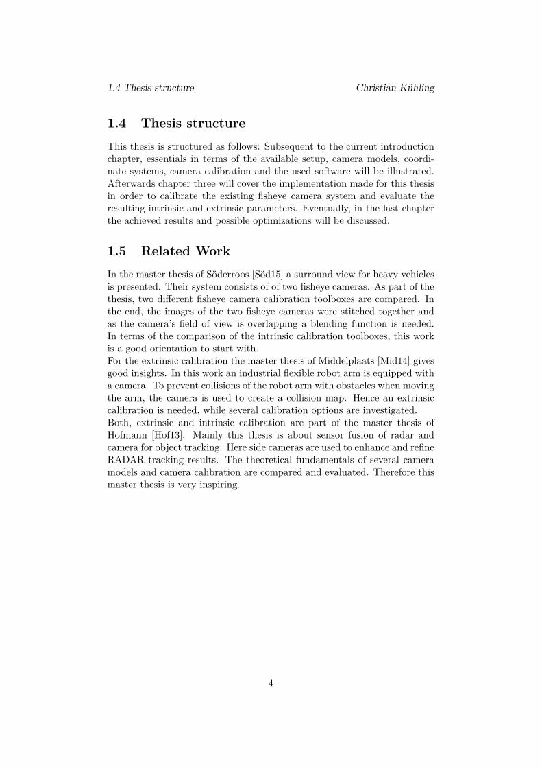
1.5 Related Work

In the master thesis of Söderroos [Söd15] a surround view for heavy vehiclesis presented. Their system consists of of two fisheye cameras. As part of thethesis, two different fisheye camera calibration toolboxes are compared. Inthe end, the images of the two fisheye cameras were stitched together andas the camera’s field of view is overlapping a blending function is needed.In terms of the comparison of the intrinsic calibration toolboxes, this workis a good orientation to start with.For the extrinsic calibration the master thesis of Middelplaats [Mid14] givesgood insights. In this work an industrial flexible robot arm is equipped witha camera. To prevent collisions of the robot arm with obstacles when movingthe arm, the camera is used to create a collision map. Hence an extrinsiccalibration is needed, while several calibration options are investigated.Both, extrinsic and intrinsic calibration are part of the master thesis ofHofmann [Hof13]. Mainly this thesis is about sensor fusion of radar andcamera for object tracking. Here side cameras are used to enhance and refineRADAR tracking results. The theoretical fundamentals of several cameramodels and camera calibration are compared and evaluated. Therefore thismaster thesis is very inspiring.

4

Chapter 2

Fundamentals

This chapter provides the basic knowledge for the further progression of thisthesis. Starting with the hardware setup [2.1] covering detailed informationabout the camera system installed in the MIG. Afterwards, the theoreticalfundamentals [2.2] like coordinate systems, the basics of camera models andfinally the essentials of intrinsic [2.3] and extrinsic camera calibration [2.4]are presented. An overview of the used libraries and software [2.5] completesthis chapter.

2.1 Hardware setup

There is a total of four cameras installed in the MIG. The first camera islocated in the front central placed between the numberplate and the car icon.Mirrored at the other end but just a little bit higher is the rear camera. Theleft and right cameras are positioned under the side mirrors of the vehicle.All cameras are displayed in detail in Figure [2.1] respectively their positionsin Figure [2.2].The BroadR-Reach SatCAM [Tec] has the following basic features and isdisplayed in [2.4a]:

• Automotive Grade Surround View Camera used in series cars as frontrear or mirror camera.

• Up to 1280x800 pixels at 30 frames per second

• Freescale PowerPC Technology

• Automotive BroadR-Reach Ethernet data transfer

• Integrated Webserver for easy configuration.

• Delivers compressed JPEG-pictures

5

2.1 Hardware setup Christian Kühling

(a) Front camera (b) Rear camera

(c) Left camera (d) Right camera

Figure 2.1: The installed camera system

(a) Front view of the MIG (b) Back view of the MIG

Figure 2.2: Camera positions

Figure [2.4b] exhibits the car trunk of the MIG. The blue box right front isthe technica engineering media gateway [Med], the switch of the BroadR-Reach cameras. In table [2.3] the BroadR-Reach SatCam’s technical data isshown.Due to restricted information its not definitely clear, but considering allavailable information the camera lenses are classified to belong to the OVTOV10645 [Omn] camera lenses family. These offer a field of view of 190◦.Based on the technical data of the camera sensors a rough model is shownin figure [2.5] to display the camera positions and their theoretical sensorcoverage in one overview. Cameras positions are marked with an orangedot. The blue area represents the area only visible to the front and rearcamera, the yellow area showing the area only visible to the left and rightcamera and at last the overlapping Fields of View are displayed in green.

6

2.1 Hardware setup Christian Kühling

Feature

Power requirement 8 to 14 Volt DC (nominal 12 Volt DC)

Size 25 x 28 x 55 mm

Weight 0,1 kg

Operation Temperature -40 to +80 degree Celsius

Figure 2.3: Technical data of BroadR-Reach SatCAM

(a) BroadR-Reach Camera [Tec] (b) Car trunk of the MIG

Figure 2.5: Overview of the camera positions and their theoretical FOVOrange Dots: camera positions. Blue area: front/rear only FOV, yellow

area: left/right only FOV, green area: overlapping FOV.

7

2.2 Theoretical fundamentals Christian Kühling

2.2 Theoretical fundamentals

In subsection [2.2.2] the coordinate systems and mathematical notations[2.2.1], that are used in this thesis, are presented. In this sections end [2.2.3]an introduction to camera systems is shown. Parts of this section werestructured based on the work presented in [BK13] and [Hof13].

2.2.1 Mathematical notations

Matrices, points and vectors are frequently used in this thesis, alongsideangles, which are particular Greek letters annotated kind of scalar. In table[2.6] the respective notations can be found.

Type Notation Explanation

Angle α Greek letter, normal font

Coordinate TA→B Bold, big letters transformstransformation from System A to B

Matrix M Bold, big letter

Point P Big letter, normal font

Scalar s Small letter, normal font

Vector ~v Small letter with an arrow above

Figure 2.6: Mathematical Notations

Coordinate representations of n-dimensional space, representing lines in n+ 1-dimensional space by adding one as a constant to the vector can bedefined as homogeneous coordinates.

xyz

→

xyz1

(2.1)

This compact combination of rotations and translations are annotated asTA→B. For arbitrary transformations from n-dimensional coordinate sys-tem A to d-dimensional coordinate system, these annotations can be used.Commonly they define a transformation matrix [2.2] consisting of a rotationmatrix R and a translation vector ~t that is used to transform homogeneouscoordinates. The rotation matrix and translation vector combined togetherare the extrinsic parameters. While the translation vector describes the posi-tion of a camera, the rotation matrix represents the rotations of the cameraregarding the yaw, pitch and roll angles. A more detailed description isexpressed later on in this thesis.

8


TA→B =

(

R ~t0 0 0 1

)

=

r11 r12 r13 t1

r21 r22 r23 t2

r31 r32 r33 t3

0 0 0 1

(2.2)

2.2.2 Coordinate systems

At some point when working with multiple cameras involving multiple co-ordinate systems, they have to be transformed to each other. To do so,mathematical notations need to be introduced. There are several coordi-nate systems used in this thesis. Starting with a world coordinate systems,which is used as a general reference. A local coordinate system which iscarried along with the motion of the vehicle is defined as the ego vehiclecoordinate system. There are two coordinate systems used by the pinholecamera model [2.2.3]: the 3-dimensional camera coordinate frame and theimage frame referencing to pixel coordinates. Following these coordinatesystems are explained in detail.

World coordinate system

The world coordinate system as shown as in figure [2.7a] defines the x-y-plane as the ground plane, while the z-axis is pointing upwards. So thecoordinate system is right-handed.

x axis

z axis

y axis

(a) World coordinate system

x

y

(b) Ego Vehicle Coordinate System,model taken from [Ego]

9


x axis

y axis

z axis

(a) Camera coordinate system

x axis

y axis

(b) Image coordinate system

Ego vehicle coordinate system

Alongside with the motion of the car, the so-called ego coordinate systemreference frame is carried along. Like the world coordinate system, it isright handed. Its origin is located in the middle of the front axle. Thex-axis points to the driving direction, the y-axis runs parallel to the frontaxle and the z-axis is pointing upwards. It is displayed in figure [2.7b].

Camera coordinate system

As shown in [2.8a], the camera coordinate systems viewpoint with the z-axispointing away from the camera in the direction of the view is the origin ofthe camera system.

Image coordinate system

Images captured from camera sensors making use of the image coordinateframe. Its center is at the top left of the position of the image and referencesto pixel coordinates.

2.2.3 Pinhole camera model

A simple model to describe the illustration properties of cameras is thepinhole camera model, which is explained in more detail in the followingworks: [MK04], [BK13] and [Sze10]. In this model, light is envisioned asentering from the scene or a distant object, but only a single ray enters froma particular point, which is “projected“ onto an imaging surface. The imageof this image plane is as a result always in focus. A single parameter of thecamera, the so-called focus length gives the size of the image relative to thedistant object. The distance from the pinhole aperture to the screen in thisidealized pinhole camera is precisely the focus length. Also, this figure [2.9a]

10


(a) Pinhole camera Model [BK13] (b) Pinhole camera Model [Sze10]

shows the distance from the camera to the object Z, the length of the objectX, the cameras focus length f and the object’s image on the imaging planex. This is summarized in equation [2.3]:

− x = f ·X

Z(2.3)

Another visualization by Szeliski [Sze10] is displayed in figure [2.9b] andillustrates the basic structure of the pinhole camera model. It shows a 3D-Point Pc, which is assumed to be in the camera coordinate system that hasits origin at Oc. This is the optical center with the axes xc, yc and zc. The3D-Point Pc is transformed onto the image sensor plane, usually by a pro-jective transformation like in equations [2.4] and [2.5]. The 3D origin Cs

and the scaling factors sx and sy determines the projected point P on thesensor plane. The last variable zc defines the so-called optical axis.

x′ =X

Z(2.4)

y′ =Y

Z(2.5)

In order to transform the 3D-Points from its own world coordinate system[2.7a] to the camera coordinate system [2.8a] equation [2.2] is used. Exam-ining the full relationship between a 3D-Point P and its image projectionx under the usage of homogeneous coordinates this results in the followingformula [2.6] [Sze10]. The Matrix K is called the intrinsic matrix, contain-ing the intrinsic camera parameters. They are needed to acquire the pixelcoordinates of the projection point (u,v). s is a scalar scaling factor. Knownas the 3 × 4 camera matrix is the combination of K[R|~t].The intrinsic camera Matrix K combines the focal lengths fx and fy togetherwith the skew γ between the sensor axes and the principal point (Cx, Cy),

11


which determines the intersection of the camera Z-axis with the viewingplane. The skew γ is usually negligible in real-world cameras, which is whyit will be assumed to be zero. Further the aspect ratio between the x-axis andy-axis can be explicit by adapting the definition of the second focal lengthfy = α fx. It is worth mentioning, that this ratio is not directly related

to the aspect ratio between an image produced by the camera (widthpx

heightpx),

but rather defines the pixel aspect ratio. Usually it is possible to simplifyfx = fy = f because of the assumption of square pixels, which means thatin most cases a single focal length is suitable. Another presumption is, thatthe principal point usually lies near the image center. This way it is possibleto get the principle point P by Px =

widthpx

2and Py =

heightpx

2.

The intrinsic camera matrix does only depend on internal camera properties,not on scene properties. So as long as parameters like focal length, whichonly changes when the lens is modified, and the output image size stays thesame, the intrinsic camera matrix can stay the same.

sx = K[R|~t]P = s

uv1

=

fx γ Cx

0 fy Cy

0 0 1

=

r11 r12 r13~t1

r21 r22 r23~t2

r31 r32 r33~t3

XYZ1

(2.6)Besides the intrinsic camera Matrix K the formula [2.6] contains the alreadyin [2.2] mentioned rotation matrix R and the translation vector ~t. Bothtogether are the extrinsic parameters and they determine the orientationrespectively the position of the camera in the world coordinate system [2.7a].The extrinsic parameters consist of six degrees of freedom, three coordinatesnamely X,Y ,Z and three angles α, β, γ. From the aviation the names roll,pitch and yaw were established for the angles [2.10].Normally rotations are done in the following order:

• Rotation around the x-axis: roll

Rx =

1 0 00 cos(γ) − sin(γ)0 sin(γ) cos(γ)

(2.7)

• Rotation around the y-axis: pitch

Ry =

cos(β) 0 sin(β)0 1 0

− sin(β) 0 cos(beta)

(2.8)

• Rotation around the z-axis: yaw

Rz =

cos(α) − sin(α) 0sin(α) cos(alpha) 0

0 0 1

(2.9)

12


Figure 2.10: Roll, pitch and yaw [Rol]

• which results in:R = RxRyRz (2.10)

13

2.3 Intrinsic camera calibration Christian Kühling

2.3 Intrinsic camera calibration

The advantage of using a wide-angle or fisheye lenses is the larger fieldof view. Though there are the disadvantages of distortion, which makesstraight lines appear as curved lines instead, and the impact on the resolutionof the image. In figure [2.11] two common types of radial distortion aredisplayed: the barrel distortion and the pincushion distortion. These typesare the most occurring distortions besides slight tangential distortion.Wide-angle cameras have a field of view(FOV) of 100◦ - 130◦ while a fisheyecamera has a larger FOV of about 180◦. Since the pinhole camera model[2.9a] can not handle a zero value on the z-coordinate, the axis parallel tothe optical axis, a lens using a classic wide angle model can not cover a 180◦

FOV. The pinhole camera model will project 3D-points covered from a 180◦

FOV at infinity and it can therefore not be used as a projection model forfisheye lenses.

Figure 2.11: Two types of distortion [Dis]

Hence new camera models that are able to handle this distortion are re-quired. These models use parameters to describe distortions. The processto estimate the set of intrisic parameters in a camera model is called in-trinsic camera calibration. Following, this section discusses three differentoptions to gain the intrinsic camera parameters and is inspired by theseworks: [Söd15], [Hof13] and [Sch].

2.3.1 Mei’s calibration toolbox

The first calibration toolbox was developed by Mei [Meia] for providing thecamera extrinsic, intrinsic and distortion parameters in MATLAB [2.5.6].It can be used to calibrate and evaluate the intrinsic camera parametersfor multiple camera types such as parabolic, catadioptric and dioptric. Thistoolbox is based on a specific projection model [Meib], an extension of [BA01]also made by Mei. Here the world points are projected onto the unit spherebefore they are projected onto the normalized image plane. This allows thecenter of projection to be shifted onto the image plane. The center of theimages are used as an estimate of the principal points with a diotric camera

14


model and a planar calibration grid is used in the calibration procedure.Figure [2.12] illustrates the projection model for projection 3D-points andis described by the following steps:

1. Project a world point Y in the camera coordinate frame onto the unitsphere

(xn, yn, zn) =Y

‖Y ‖(2.11)

2. Change the points to a new reference frame centred in Cp = (0, 0, ξ)

(xS , yS , zS) = (xn, yn, zn + ξ) (2.12)

ξ =df

√

df2 + 4p2(2.13)

where df is the distance between focal points and 4p is the lactus rec-tum, the chord through a focus parallel to the conic section directrix.

3. Project the points onto the normalised image plane. The shift of thecenter of projection in the previous step ensures, that ZS is never zeroand this perspective projection runs smoothly.

Mu = (xS

zS

,yS

zS

, 1) (2.14)

4. Add the radial distortion to the point, where ki are the distortionparameters, and D is the distortion function [2.17].

Md = Mu + D(Mu, ki) (2.15)

5. Project the points onto the image using the camera matrix K

P =

f s xc

0 fα yc

0 0 1

md (2.16)

Equation [2.17] shows the distortion function D with distortion pa-rameters ki = 1, .., 5 and p =

√

x2 + y2

D(p) = 1 + k1p2 + k2p4 + k3p6 + k4p8 + k5p10 (2.17)

It is required to collect images of the chessboard calibration pattern shownin different positions and angles to the camera before using the toolbox.The user has to select at least three non-radial points, meaning not placedon radii from the image center, which belong to a line in an image, andthe focal length is estimated from them. Also, the user has to select fourgrid corner points in each image which can be used for initialization of the

15


Figure 2.12: 2D illustration of Mei projection model [Söd15]

extrinsic grid parameters. Afterwards, the grid pattern is reprojected anda global minimization can be done when calibrating the intrinsic cameraparameters.Unfortunately, this calibration toolbox is not working automatically becausethe user has to select and click on the four outer grid corners in everyimage. Also, it is not possible to relocate the position of a displaced cornermanually. Therefore images, which work poorly with the corner detectionshould be removed from the calibration dataset. In addition MATLAB[2.5.6] is required to use this tool and for that, a charged license is needed.Because of these drawbacks, Mei’s calibration toolbox cannot be part of aneasy-to-use calibration script.

2.3.2 Scaramuzza’s OcamCalibToolbox

Another calibration toolbox for MATLAB has been provided by Scaramuzza[OCa] based on his work [SMS06]. It can be used for any central omnidi-rectional cameras including fisheye lenses. There are similarities to Mei’stoolbox, because both require MATLAB, make use of the chessboard cali-bration pattern and can be used for calibrating the intrinsic and the distor-tion parameters. The user needs to collect some images of the calibrationpattern shown in different angles and positions. An advantage over Mei’stoolbox is the possibility to detect the corners automatically instead of man-ually proceeding. In a case of a faulty automatically detection the cornerspositions can also be changed manually. A disadvantage of this toolbox is,that coordinate system is defined differently regarding not using the stan-dard right-handed coordinate system. When using the calibration results interms of rotation and translation this has to be corrected.Mathematically the simple pinhole camera model [2.2.3], even incorporatingdistortions, is not able to model field of views with angels larger than 180◦.Already with much smaller angles problems can occur in practice. That is

16


why Scaramuzza presented a new camera model [SMS06] which allows higherviewing angles. Systems exhibiting strong radial distortion like mirror lensoptics(catadioptric) [2.13b], wide angle [2.13c] and fisheye lenses [2.13a] canbe used with the proposed approach. Those distortions can be recognized infisheye lenses when the middle of the image has a higher zoom factor thanthe edges. Because of these distortions, relative sizes change and straightlines become bent.

(a) fisheye (b) Catadioptric system (c) Wide angle

Figure 2.13: Images taken with different optics [Hof13]

Scaramuzza’s model does not simply reposition the pixels on the image plane

with a distortion function. Instead it computes a vector(

x y z)T

radiat-

ing from the single viewpoint to an picture sphere pointing in the direction

of the incoming light ray for each pixel position(

u v)T

. This reference

frame originates in the center of the image. In figure [2.14] the differenceof the central projection used in the standard pinhole camera model [2.2.3]and the model by Scaramuzza is shown.

Function g(p) [2.18] is defined as a Taylor polynomial and models the radialdistortion. It consists of coefficients ai which define the intrinsic parameters

and the Euclidean distance of the pixel position(

u v)T

from the image

center through function [2.19]. Function [2.18] is needed to make use of thespherical projections properties, so that a point in camera coordinates canalways be represented as a point on a specific ray. This is shown in equation[2.20] with s being an arbitrary scaling factor.

g(p) = a0 + a1p + a2p2 + a3p3 + .. + anpn (2.18)

p =√

u2 + v2 (2.19)

xyz

= s

uv

g(p)

(2.20)

17


(a) The standard pinhole cameramodel

not distinguishing scenepoints lying on opposite

half-lines

(b) The spherical model

distinguishing two scenepoints lying on opposite

half-lines

Figure 2.14: Scaramuzza perspective projectionlimited to view angles covered by the projection plane and spherical

projection which covers the whole camera reference frame space [Sca07].

To project a point from camera coordinates onto an image, equation’s [2.18]polynomial has to be solved, in order to get u and v. That is computa-tionally inefficient. So Scaramuzza estimated an inverse Taylor polynomial[2.21]. The radial positioning on the image plane based on the angle α ofa light ray to the z axis is described by it. Just like Mei’s toolbox [2.3.1],Scaramuzzas requires MATLAB. Since there is no full-automatically possi-bility to calibrate the cameras and license costs of MATLAB, this toolboxis insufficient for an easy-to-use calibration script.

f(α) = b0 + b1α + b2α2 + b3α3 + .. + bnαn (2.21)

r =√

x2 + y2 (2.22)

α = arctan(z/r) (2.23)

u =x

rf(α) (2.24)

v =y

rf(α) (2.25)

2.3.3 OpenCV camera calibration

The widely used open source computer vision library OpenCV [2.5.2] pro-vides a intrinsic camera calibration tool. It is based on Brown’s [Sze10]distortion model. The coordinates x′ [2.4] and y′ [2.5] are the ideal pinholecamera coordinates. x′′ and y′′ are their respective repositioning based onthe distortion parameters. Those are k1, k2, k3 and the tangential distortioncoefficients p1 and p2. Those calculated coordinates are sufficient for most

18


and weaker distortions, but in case of stronger ones the first term of [2.27]and [2.28] are divided by 1 + k4r2 + k5r4 + k6r6 where k4, k5 and k6 areadditional distortion coefficients.

r2 = x′2 + y′2 (2.26)

x′′ = x′(1 + k1r2 + k2r4 + k3r6) + 2p1x′y′ + p2(r2 + 2x′2) (2.27)

y′′ = y′(1 + k1r2 + k2r4 + k3r6) + p1(r2 + 2y′2) + 2p2x′y′ (2.28)

u = fx · x′′ + cx (2.29)

v = fy · y′′ + cy (2.30)

Especially for fisheye lenses this model has been adjusted [Opeb] in OpenCVversion 3. Subsequent the OpenCV 3 fisheye camera model is explained. Inequation [2.31] the coordinate vector ~xc of a point P in the reference frame isshown. This point P is a point in 3D coordinates X in the world coordinatesystem, which is stored the matrix X. The matrix R is the rotation matrixcorresponding to the rotation vector ~om: R = rodrigues(om) [Gup89].Since the point P is a point in 3D coordinates it consists of 3 coordinatesx = ~xc1

, y = ~xc2, z = ~xc3

.~xc = RX + T (2.31)

The pinhole projection coordinates of P is(

a b)T

where a = x/z, b =

y/z, r2 = a2 + b2 and θ = arctan r. Equation [2.32] describes the fisheyedistortion:

θd = θ(1 + k1θ2 + k2θ4 + k3θ6 + k4θ8 (2.32)

This results in the distorted point coordinates(

x′ y′

)Twhere

x′ = (θd/r)x (2.33)

y′ = (θd/r)y (2.34)

Finally the conversion into pixel coordinates with the resulting vector(

u v)T

whereu = fx(x′ + αy′) + Cx (2.35)

andv = fyyy + Cy (2.36)

The actual calibration method is based on the work of Zhang [Zha00] andBouguet [Bou15]. A known pattern has to be printed like in figure [2.15a]on a piece of paper and attached to a rigid surface to make it reasonablyplanar. Information like the used calibration pattern, the size of its circlesor corners and the pure amount of circles or corners must be known.

19


(a) Chessboard calibration pattern(b) Asymmetric circles calibration pat-tern [pat]

Figure 2.15: Calibration patterns

(a) Original fisheye image (b) Complete rectified fisheye image

Figure 2.16: Fisheye image rectification [Opec]

To calibrate one camera it takes several images of the calibration pattern invarious orientations. In the process either the calibration pattern or like inthis case the camera must be fixated while moving the other one around. Ineach image the feature points of the pattern have to be detected by a patternspecific feature detection algorithm like the algorithm for chessboards byBennett [BL14].Since the intrinsic and the distortion parameters depend on the camera andits lens, it is not essential to calibrate all wanted cameras at once.Accompanied by the rectification of curved images is the loss of outer partsof the original fisheye image. Figure [2.16] exhibits an original fisheye imageand its completely rectified version. Only the inner tagged rectangle of theimage is further used, the rest of the image is excised.OpenCV’s camera calibration is robust, works with multiple calibration pat-terns and runs automatically. Hence it is a good choice for a camera cali-bration script.

20

2.4 Extrinsic camera calibration Christian Kühling

2.4 Extrinsic camera calibration

Analogous to intrinsic camera calibration, the process to estimate the setof extrinsic parameters in a camera model is called extrinsic camera cali-bration. The extrinsic parameters of a camera are the camera’s position,described through the translation vector ~t and its orientation, displayed viathe rotation matrix R as already introduced in [2.2.1].When multiple cameras are used, like in this thesis, the camera’s extrinsicparameters have to be recalibrated, if their position relative to each other ischanged. Fortunately, the used broadreach-cameras are firmly installed sothat only an extraction and renewed installation or strong impacts wouldmake this necessary.It is important to estimate the extrinsic parameters for each of the camerasin relation to the same reference coordinate system. This way the transfor-mation between all cameras can be estimated.Because the relation between the cameras is crucial here, it is an easy possi-bility to place the reference system in one of the cameras. Thus, the positionsof the other cameras can be estimated in relation to the first one.There are many ways to calculate the extrinsic parameters of a camerasystem. Subsequent works providing options to gain the extrinsic parametersare presented.

2.4.1 Approaches

There are several options available for calculation the extrinsic camera pa-rameters. First of all the most obvious: measuring of the translation androtations manually. This is only possible, if the cameras are exposed, likethe front [2.1a], left [2.1c] and right [2.1d] camera of the MIG, but unlikethe rear camera [2.1d]. The body of the last-mentioned is not visible at all,only the camera’s lense can be seen. Hence no reasonable assertions can bemade about this cameras rotation.An often used approach to determine the extrinsic camera parameters is theuse of markers. Just like the calibration patterns used for intrinsic calibra-tion [2.15], the algorithms recognize the predefined forms of the marker.The work of Vatolin, Strelnikov and Obukhov [OSV08] presents an approachto fully automatic pantilt-zoom (PTZ) camera calibration, using a visualmarker detection system. It focuses on extrinsic parameters only. A set ofmeasurements, each represented by the correspondence between the Carte-sian work coordinates and the camera’s internal coordinates for a givenpoint, is used. The camera position and rotation can be calculated inde-pendently because this approach uses a "direct measurement". The abovementioned visual marker are detected via a corresponding detection sys-tem to obtain the world coordinates of specific points, even though internalcoordinates are accessible in most cameras. Unfortunately, this approach

21


(a) ARTag visual marker acting as a cal-ibration object [OSV08]

(b) AR markers used to calibrate robots[Rak16]

requires fixed camera positions and is meant to be used for indoor camerasas can be seen in figure [2.17a], thus adjusting this work for this thesis needswould take have been elaborate.In the master thesis [Rak16] multiple approaches to get extrinsic parame-ters were compared to each other. ROS [2.5.1] was used, just like in thisthesis working group. That is why, it gives an insight, especially because be-sides AR(Augmented Reality) marker were used besides point clouds; moreconcretely the ROS library ar_track_alvar. The results of this thesis werepromising, but unfortunately when testing this library with the existinghardware got problems with false positive marker recognition.A completely different technique is presented in the work of Takahashi,Bobuhara and Matsuyama [TNM12]. This paper assumes that there is nodirect visibility to a 3D reference object. So this reference object is capturedvia a mirror under three different unknown poses. Afterwards the extrinsicparameters are calibrated from 2D appearances of the appropriate reflec-tions in the mirror. Since the cameras of the MIG can have direct visibilityto reference objects, this is not worth taking a deeper look.A very fast approach has been made in a paper called "extrinsic calibrationof a set of range cameras in five seconds without pattern" [FMGJRA14].It relies on finding and matching planes. The presented method serves tocalibrate two or more range cameras, requiring only to observe one planefrom different viewpoints simultaneously. According to its authors, thisapproach is very fast. It is generic, because it does not require a 3D cali-bration pattern or relies on the robustness of simultaneous localization andmapping (SLAM) or Visual Odometry(VO), which highly depends on theenvironment. Though this works takes advantage of the fact, that struc-tured environments like floors, walls and ceiling contain large planes, so ismade for indoor camera calibration, similar to [OSV08] and therefore it isno option for this thesis.In the work [TR13] by Raúl Rojas and Ernesto Tapia the pattern of appar-

22


ent motions of objects or surfaces in a visual scene caused by the relativemotion between an observer and a scene is the base for extrinsic calibration.This is called optical flow. Here it is assumed, that the camera is mountedon a moveable object like a robot or a vehicle while pointing forward. Nextthis object is moving forward and sideways on a flat area to acquire the im-ages needed for the calibration. This way a subset of the segments definedby the optical flow are the projection of parallel line segments of the worldcoordinate frame. At a common point, the so called vanishing point, this setof parallel lines intersects in the image plane. If the vehicles moves sidewayswhile still capturing the video frames, the set of vanishing points define thehorizon. According to this promising work, estimating the direction andposition of the camera is possible, if the slope of horizon line and the coor-dinates of vanishing points of lines parallel to the forward movement of thevehicle is known.Since this approach requires forward pointing cameras it could have beenused for the front camera only or most probably the rear camera as well.Therefore it is not possible to get extrinsic parameters for rest of the camerasystem. So this calibration method was not chosen.

The work [CAD11] written by Davison, Angeli and Carrera is based on thewidely used Simultaneous Localization and Mapping (SLAM) algorithm. Itis used on automatically extrinsic calibrate a mulit-camera rig. The samealgorithm is part of the chosen extrinsic calibration pipeline CamOdoCal[2.4.2]. No calibration pattern, overlapping fields of view or other infrastruc-ture is required. Known individual intrinsic parameters and synchronisedcapture across the multiple cameras are assumed, although they can havevarying types and optics and uses a multi-camera rig mounted on a mobilerobot. The approach has the following steps:

• Attachment of the cameras to a mobile robot in arbitrary rigid posi-tions and orientations.

• Pre-programmed movement of the robot through an unprepared envi-ronment. Meanwhile the synchronized video streams from the camerasare captured.

• Every cameras video stream is analysed by a modified version of theMonoSLAM algorithm [DRMS07]. This is visualized in figure [2.18].MonoSLAM builds a 3D map of visual feature locations, while ev-ery feature is characterized by a SURF(Speeded Up Robust Features)descriptor. Also the camera motions are estimated.

• By using bundle adjustment, each camera’s map and motion estimatesare individually refined.

23


Figure 2.18: MonoSLAM. Top: in operation. Bottom: SURF featuresadded. [CAD11]

• Via thresholded matching between their SURF descriptors, candidatefeature correspondences between each pair of individual maps are ob-tained.

• To generate hypotheses, sets of three correspondences between mapsfrom the SURF [BTVG06] matches are used. These sets in combi-nation with RANSAC [FB81] and 3D similarity alignment is used, toachieve an initial alignment of the maps’ relative 3D pose and scale.Afterwards a reliable set of correspondences between each pair of mapsis derived, which satisfies descriptor matching and geometrical corre-spondence. The monocular maps are merged into a single joint map.

• In the end, full bundle adjustment optimization with this initial jointmap as the starting point is run to estimate the relative poses of thecameras, 3D positions of scene points and motion of the robot.

Overall results of this approach are satisfying. That is why in this thesisthe further developed pipeline CamOdoCal [2.4.2] is part in the subsequentimplementation.

24


2.4.2 CamOdoCal

One of the key aspects of this thesis’s goal is camera calibration and hencealso the calculation of extrinsic parameters. Therefore within this thesis,an easy-to-use calibration script has to be implemented, which has some re-quirements. The user interaction should be minimized and optimally thereshould not be any expenses for the requirement tools. Hence open sourceapplications are preferred. Therefore this thesis uses CamOdoCal(CameraOdometry Calibration) for calculating the extrinsic parameters. It is anopen source pipeline written in C++, available at GitHub [Cam] and isbased on the work of Heng, Li and Pollefeys [HLP13] as part of the au-tonomous car project V-charge of the ETH-Zürich. CamOdoCal is the basefor further works like [HFP15]. The pipeline is able to calculate both in-trinsic and extrinsic parameters. Though the intrinsic calibration is verysimilar to the one provided by Mei [2.3.1], only the extrinsic calibration willbe discussed. The name of the framework directly tells which data is usedfor calibration: camera images and wheel odometry. These data has to berecorded while driving around with the vehicle for a short time at a richtextured environment. The extrinsic calibration finds all camera-odometrytransforms, is unsupervised and uses natural features. Another advantageof CamOdoCal over the other approaches is its flexibility, because it is ableto compute and handle parameters of the pinhole camera model [2.2.3], theunified projection model [2.3.1] and the equidistant fisheye model [KB06].In short, CamOdoCal does the following steps when calibrating the extrinsicparameters:

1. Visual odometry for each camera

2. Triangulate 3D points with feature correspondences from mono visualodometry and run bundle adjustment

3. Run robust pose graph simultaneous localization and mapping (SLAM)and find inlier 2D-3D correspondences from loop closures

4. Find local inter-camera 3D-3D correspondences

5. Run bundle adjustment

Ensuing, a more detailed summary of the single steps strongly based on theCamOdoCal paper [HLP13] is presented.

Monocular visual odometry

First for each camera separately monocular visual odometry with slidingwindow bundle adjustment is run. Visual odometry is the process of deter-mining the orientation and position of an moving object, that has a cameraaffixed like a robot or a vehicle, by analyzing its camera images. In the work

25


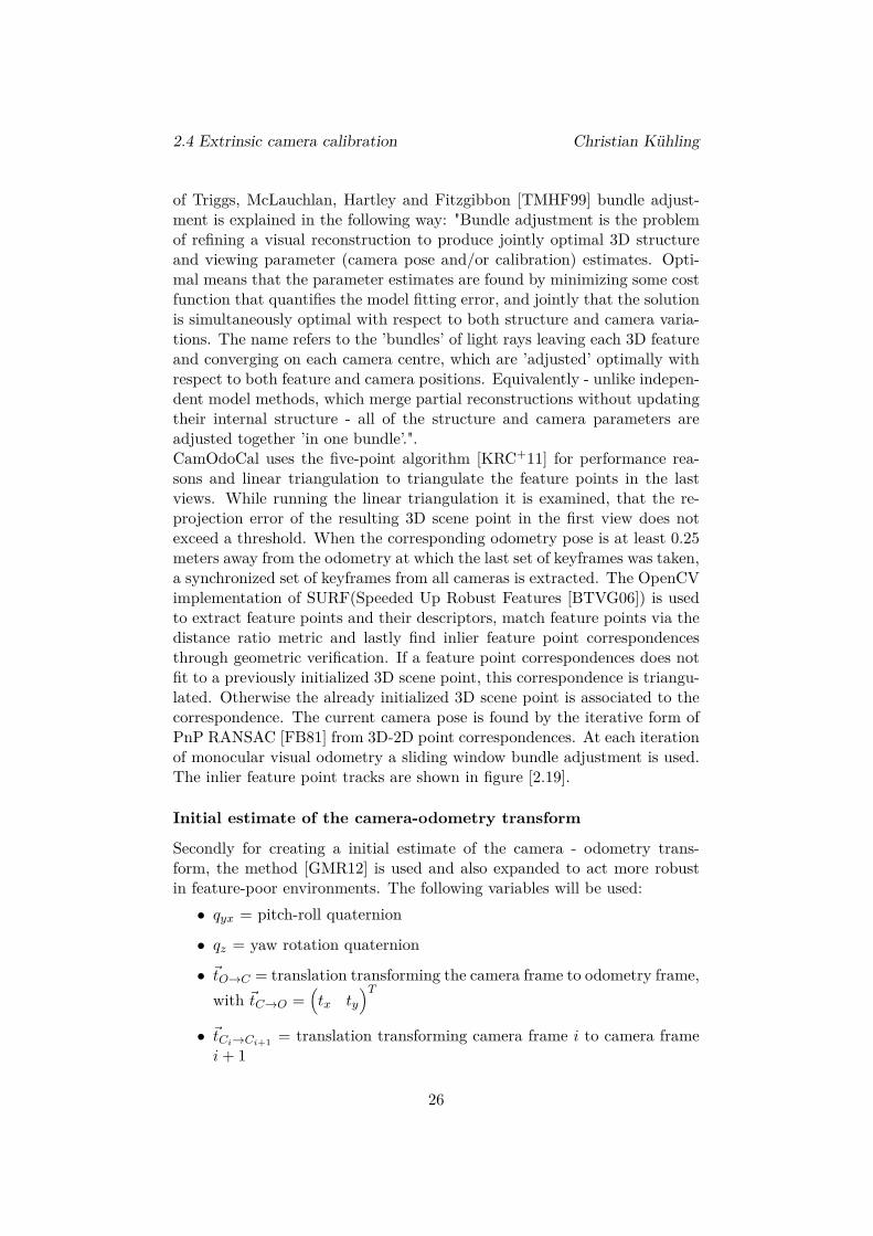
of Triggs, McLauchlan, Hartley and Fitzgibbon [TMHF99] bundle adjust-ment is explained in the following way: "Bundle adjustment is the problemof refining a visual reconstruction to produce jointly optimal 3D structureand viewing parameter (camera pose and/or calibration) estimates. Opti-mal means that the parameter estimates are found by minimizing some costfunction that quantifies the model fitting error, and jointly that the solutionis simultaneously optimal with respect to both structure and camera varia-tions. The name refers to the ’bundles’ of light rays leaving each 3D featureand converging on each camera centre, which are ’adjusted’ optimally withrespect to both feature and camera positions. Equivalently - unlike indepen-dent model methods, which merge partial reconstructions without updatingtheir internal structure - all of the structure and camera parameters areadjusted together ’in one bundle’.".CamOdoCal uses the five-point algorithm [KRC+11] for performance rea-sons and linear triangulation to triangulate the feature points in the lastviews. While running the linear triangulation it is examined, that the re-projection error of the resulting 3D scene point in the first view does notexceed a threshold. When the corresponding odometry pose is at least 0.25meters away from the odometry at which the last set of keyframes was taken,a synchronized set of keyframes from all cameras is extracted. The OpenCVimplementation of SURF(Speeded Up Robust Features [BTVG06]) is usedto extract feature points and their descriptors, match feature points via thedistance ratio metric and lastly find inlier feature point correspondencesthrough geometric verification. If a feature point correspondences does notfit to a previously initialized 3D scene point, this correspondence is triangu-lated. Otherwise the already initialized 3D scene point is associated to thecorrespondence. The current camera pose is found by the iterative form ofPnP RANSAC [FB81] from 3D-2D point correspondences. At each iterationof monocular visual odometry a sliding window bundle adjustment is used.The inlier feature point tracks are shown in figure [2.19].

Initial estimate of the camera-odometry transform

Secondly for creating a initial estimate of the camera - odometry trans-form, the method [GMR12] is used and also expanded to act more robustin feature-poor environments. The following variables will be used:

• qyx = pitch-roll quaternion

• qz = yaw rotation quaternion

• ~tO→C = translation transforming the camera frame to odometry frame,

with ~tC→O =(

tx ty

)T

• ~tCi→Ci+1= translation transforming camera frame i to camera frame

i + 1

26


• ~tOi→Oi+1= translation transforming odometry frame i to odometry

frame i + 1

• sj = scale for each of the m sparse maps

• qOi→Oi+1= unit quaternion rotating odometry frame i to odometry

frame i + 1

• qCi→Ci+1= unit quaternion rotating camera frame i to camera frame

i + 1

• qC→O = unit quaternion rotating camera frame to odometry frame,with qC→O = qzqyx

A quaternion can be thought of a composite of a scalar and a vector, avector with four components, or as a complex number with three differentimaginary parts [Hor87]. It is possible to convert between a rotation matrixand a quaternion [K+99]. Since quaternions are more compact than rotationmatrices, they are used as a representation of rotations in this subsection.The hand-eye calibration problem consists of calculating the rotation andtranslation between a sensor like a camera on a robot actuator and theactuator itself [HD95]. It is described using quaternion representation isdescribed via equations [2.37] and [2.38].

qOi→Oi+1qC→O = qC→OqCi→Ci+1

(2.37)

(R(qOi→Oi+1) − I~tC→O) = sjR(qC→O)~tCi→Ci+1

− ~tOi→Oi+1(2.38)

Rotations around the z-axis commute. This is used to estimate the pitch-rollquaternion by substituting qC→O = qzqyx, as shown in equation [2.39].

qOi→Oi+1qyx − zyxqCi→Ci+1

= 0 (2.39)

There are two constraints on the unknown qyx. The first constrain: thex-value and y-value of the pitch-roll quaternion multiplied with each otherequals the negative z-value multiplied with the w-value of the same pitch-roll quaternion. The second constrain: the transposed pitch-roll quaternionmultiplied with the original one equals one. These constrained are mathe-matically expressed in equation [2.40] respectively [2.41].

qyxxqyxy

= −qyxzqyxw

(2.40)

qTyxqyx = 1 (2.41)

With at least two or more motions a 4n × n matrix T [2.43] is build:

T =(

S1T ... Sn

T)T

(2.42)

27


where S is a 4 × 4 matrix resulting of equation [2.38]. With the unitarymatrix U the singular value decomposition is found: T = USV T . Thenull space of T is encompassed by the last two columns of V: the last tworight-singular vectors ~v3 and ~v4, as displayed in equation [2.43].

qyx = λ1 ~v3 + λ2 ~v4 (2.43)

Finally qyx is obtained by using the constraints [2.39] and [2.40] to solve forλ1 and λ2.

Due to planar motion, the z-component of the camera-odometry transla-tion is unobservable. So the third row from equation [2.38] can be removed,resulting in equation [2.44].

(

cos β − 1 − sin βsin β cos β − 1

)(

tx

ty

)

− sj

(

cos α − sin αsin α cos α

)(

p1

p2

)

+ ~t′

Oi→Oi+1= 0

(2.44)Here, α is the yaw, ~t′

Oi→Oi+1denotes the first two elements of the translation

vector ~tOi→Oi+1and

(

p1 p2

)Tare the first to elements of the vector R(qyx).

With J =

(

cos β − 1 − sin βsin β cos β − 1

)

and K =

(

p1 −p2

p2 p1

)

equation [2.44] is

rewritten as a matrix vector equation in equation [2.45].

(

J K)

tx

ty

−sj cos α−sj sin α

= −~t′

Oi→Oi+1(2.45)

Afterwards the 2n × (2 + 2m) matrix G is build in [2.46], with n =m∑

i=1

ni

because of m visual odometry segments with n1 ≥ 2, ..., nm ≥ 2 motionseach. J

ji and K

ji are the respective versions of J respectively K to the ith

motion in the visual odometry segment j.

G =

J11 K1

1 ... 0 0 ... 0 0... ... ... 0 0 ... 0 0

J1n1

K1n1

... 0 0 ... 0 0

0 0 ... Jj1 K

j1 ... 0 0

0 0 ... ... ... ... 0 0

0 0 ... J jnj

Kjnj

... 0 0

0 0 ... 0 0 ... Jm1 Km

1

0 0 ... 0 0 ... 0 00 0 ... 0 0 ... Jm

nmKm

nm

(2.46)

28


Figure 2.19: Inlier feature point tracks [HLP13]

Using Matrix G [2.46] equation [2.45] is extended and rewritten to involvethe motions of the visual odometry segements in equation [2.47]:

G

tx

ty

−s0 cos α0

−s0 sin α0

...−sm cos αm

−sm sin αm

= −

~t′

O0→O1

...~t′

On→On+1

(2.47)

Now, to find the solution to ~tC→O =(

tx ty

)T, sj and αj , the least square

motion is used. This estimates the scale sj for each visual odometry segmentbesides the translation vector ~tC→O, but still there are m hypotheses ofα. The best hypothesis that minimizes the cost function [2.48] is chosen,before the estimate of sj , α, qyx and ~tC→O are refined by using non-linearoptimization to minimize the just mentioned cost function C [2.48].

C =

nj∑

i=0

((R(qOi→Oi+1) − I)~tC→O − sjR(α)R(qyx)~tCi→Ci+1

+ ~tOi→Oi+1)

(2.48)

3D point triangulation

In the third step, all features of every frame which are visible in the currentframe and the last two frames, and do not correspond to a previously ini-tialized 3D scene point are found for each camera while iterating through

29


Figure 2.20: Inlier feature point correspondences between rectified images

every frame. Each feature correspondence in the last and current frameis triangulated. If a threshold of 3 pixels for the reprojection error of theresulting 3D scene point in the second last frame does not exceed, this 3Dscene point is associated with the corresponding feature in the second lastframe. Afterwards, each feature track is associated with the same 3D scenepoint which the first three features already correspond to. To optimize theextrinsic parameters and 3D scene points, bundle adjustment is run via theCeres solver [AM12]. This minimizes the image reprojection error across allframes for all cameras.

Finding inter-camera feature point correspondences

As the fourth step, a local frame history for each camera is retained by iter-ating over each odometry pose of increasing timestamp. For every possiblepair of cameras at each odometry pose the features in the first camera’s cur-rent frame are matched against those in the second camera’s frame history.This is done to find the frame in the history that provides the highest num-ber of inlier feature points correspondences. The image pair is rectified on acommon image plane which corresponds to the average rotation between thefirst camera’s pose and the second camera’s pose before the feature match-ing. By using the current extrinsic estimate and odometer poses, the cameraposes are calculated. The rectification is done to ensure a high number ofinlier feature point correspondences. In figure [2.20] an example of a rectifiedimage pair between two cameras is shown. By reprojecting 3D scene pointsin the map corresponding to the first camera into the first rectified frameand equally for the second camera, the subset of inlier feature correspon-dences that correspond to 3D scene points found in the map. If a thresholdof 2 pixels is exceeded by the image distance between the feature pointsand corresponding projected 3D scene point, the feature correspondence isrejected. This is done for each inlier feature correspondence.

Loop closures

The penultimate step is loop closures detection. This is done for enhancingthe robustness of the just applied SLAM algorithm [Loo]. The loop closure

30


problem consists in detecting when the vehicle or robot has returned toan already visited location after having discovered new areas for a while.It is possible to increase the precision of the current pose estimate. Inthis case, it is also a mutual verification between the poses calculated byCamOdoCal and the odometry poses. Following is done for each frame foreach camera. Features of the corresponding image are converted into a bag-of-words vector and this vector is added to a vocabulary tree, whereby aDBoW2 [GLT12] implementation is used. The n most similar images arefound. Then the matched images, which belong to the same monocularvisual odometry segment and whose keyframe indices are within a certainrange of the query images keyframe index are filtered, to avoid unnecessarylinking of frames whose features may already belong to common featuretracks.

Full bundle adjustment

Lastly full bundle adjustment is performed, optimizing all extrinsic param-eters, odometry poses and 3D scene points.Because the z-component of the camera-odometry translation is unobserv-able due to planar motion, the relative heights of the cameras are onlyestimated, hence a hand measurement is recommended.

31

2.5 Used libraries and software Christian Kühling

2.5 Used libraries and software

This section introduces the libraries and software used in this thesis.

2.5.1 ROS

ROS stands for Robot Operating System and is a modular framework forrobotic software projects. It provides package management, IPC (inter-process communication) and hardware abstraction. The communication be-tween the components is message-based. Using the publish-subscribe pat-tern, each component (or node) can subscribe to so-called topics and pushmessage to them. The structure of a message is defined static. It composesdifferent fields of primitive types, arrays of primitive types and other mes-sages. ROS also offers so-called nodelets, that act similar to nodes. Justlike when comparing threads to processes, nodelets have the advantage overnodes of zero copy costs between nodelets of the same nodelet handler. Sothere are no costs of copying or serialization between nodelets of the samenodelet handler, despite running different algorithms. Recordings of ROSnodes, for example of images captured by a camera, are called rosbags.Hence the working group autonomous cars of this thesis is mainly usingROS, it is mandatory using it for this thesis. All implementations createdfor this thesis have the option to be run as a nodelet or as a node.

2.5.2 OpenCV

OpenCV [Opea] stands for Open Source Computer Vision Library. It is anopen source library for machine learning and computer vision. The sourcecode of OpenCV is available at GitHub [Oped]. Hence it is easy to modifythe code for specific needs. It was built to provide a common infrastructureto accelerate the use of machine perception and a common infrastructure forcomputer vision. Well-established companies like Google, Microsoft, Intel,Sony or IBM employ the library. There are C++, C, Python, Java andMATLAB interfaces available and the library supports Microsoft Windows,Linux, Android and Mac OS. Thanks to taking advantage of MMX, SSEinstructions when they are available alongside with CUDA and OpenCL in-terfaces, mostly real-time vision applications are possible. This thesis usesOpenCV as a dependency of CamOdoCal [2.4.2], its intrinsic camera calibra-tion implementation [2.3.3] and its algorithms to rectify images which wereintroduced in version 3.0 alongside many other functionalities for fisheyecamera lenses.

2.5.3 LibPCAP

LibPCAP [Libc] is a portable C/C++ library for network traffic capture.Functionally, it is the sibling of its Windows pendant WinPCAP [Win].

32


PCAP stands for packet capture and is used to get direct access to packetsfrom the network interface. Famous tools using LibPCAP are TCPdumpand Wireshark [Wir]. LibPCAP purpose in this thesis implementation isestablishing a connection between the installed camera system [2.1] andROS [2.5.1] via TCP/IP.

2.5.4 LibJPEG-turbo

Due to our focus on image calibration, an efficient image processing processis obviously indispensable. Libjpeg-turbo [Libb] is a huge improvement overthe widely used libJPEG [liba]. It is a JPEG image codec, which uses SIMDinstructions like MMX and SSE2 to accelerate baseline JPEG compressionand decompression on modern systems like x86, x86-64 and ARM. LibJPEG-turbo is generally two up to six times faster as libJPEG, or on other systems,it is as least equal. It even outperforms other rivals using proprietary high-speed JPEG codes in many cases, thanks to its highly optimized Huffmancoding routines. LibJPEG-turbo has the traditional libJPEG API, as well asthe less powerful but more straightforward TurboJPEG API implemented.In this thesis it is used for decompressing the compressed JPEG images, thecameras are sending over the network.

2.5.5 Docker

Docker [Doca] is a software container platform. When using container, ev-erything required to make a piece of software run is packed into isolatedcontainers. Because of that, it is not necessary to install all required depen-dencies on a running real existing machine with the possibility to generateconflicts. This way a container grants stability. While virtual machinesbundle a full operating system, Docker containers only bundle the requiredlibraries and settings required to make the software work. In consequence,the software will run the same, regardless of where it is deployed. Docker isavailable for Linux, Microsoft Windows and Mac OS. All in all Docker con-tainers are efficient, lightweight and self-contained systems. Hence Dockercontainers are a logical choice for this thesis because ROS [2.5.1] using onlya trimmed version of OpenCV [2.5.2] can conflict with a full installation ofOpenCV, that is required by CamOdoCal [2.4.2].

2.5.6 MATLAB

Similar to OpenCV [2.5.2] MATLAB [Mat] is a software environment formathematical calculations, widely used in science and engineering, partic-ularly for machine learning, signal processing, image processing, computervision, robots and more. The name MATLAB stems from its optimizationfor matrix calculations (Matrix Laboratory). Nonetheless, in the mean-while MATLAB has also been used in statistics, economic optimization and

33


modeling, or biological problems. MATLAB has two advantages concerningthis thesis: multiple available calibration libraries like Mei’s toolbox [2.3.1]and Scaramuzza’s toolbox [2.3.2] are implemented using MATLAB and werethus easy to adopt. Also, MATLAB is a rigorously tested environment usedin many production settings. Thus it is both reliable for future use andscalable when later used on larger machines/clusters. But it has also twodisadvantages: its license costs and that both toolboxes cannot be run com-pletely automatically. Therefore MATLAB is only used to get additionalinsights but not as part of the implementation.

34

Chapter 3

Implementation

After introducing the fundamentals of camera calibration in the previouschapter [2] the upcoming chapter covers the made implementations in orderto achieve this thesis goals [1.3] in chapter [1]. At the beginning of thisthesis the cameras were installed and wired, but there was no possibility toget the camera’s pictures and consequently no link to the used framework.So the first essential part of the implementation is to write a camera driver[3.1]. Since the cameras are sending compressed JPEG-Images over thenetwork [2.1] and decompression is time-consuming and produces a highcomputational load it is advisable to implement an efficient ROS node [2.5.1]only for decompression [3.2]. These are the preparations of the thesis.The actual camera calibration is done by an easy-to-use camera calibrationscript [3.3]. The calculated intrinsic and extrinsic camera parameters arethen used to rectify the fisheye images [3.4], provide those images and tocreate a surround view [3.5] of the MIG.

3.1 The camera driver

When using the cameras for the very first time, their VLAN(virtual localarea network) configuration must be adjusted to prevent interferences insidethe existing LAN of the MIG. Conveniently this can easily be done via theintegrated web interface. Once the BroadR-Reach cameras are switched on,they are constantly sending DHCP(dynamic host configuration protocol)requests.Under the usage of the libPCAP library [2.5.3] the driver responses to thisrequest with specific network packets. Because libPCAP is a C library thecamera driver is written in C++. As a result, every camera gets its own fixedIP address and starts sending compressed JPEG pictures. This is happeningthrough one ROS node for each camera with adjusted configurations whichcontains the IP address, the MAC(Media access control) address, an URLto the camera info file, the cameras name for each camera and the network

35

3.2 Decompression of received compressed JPEG images Christian Kühling

interface to use. The MAC address is the cameras constant hardware addressand, because the TCP-IP protocol is used, the destination of the DHCPresponse packet.The camera info file comprises the following information about each camera:

• Image width

• Image height

• Camera matrix

• Distortion model

• Distortion coefficients

• Rectification matrix(stereo cameras only)

• Projection matrix

This information are published with the aid of the ROS camera info manager.Other ROS nodes can subscribe to this topic to get the depicted intrinsiccalibration.Due to the allocation of the IP-addresses, each camera is constantly sendingcompressed JPEG-Packets. One single image cannot be sent within onepacket because of TCP-IP limitations. Here one image consists of roughlyninety packets. Therefore the driver differs between the start of a new imagewith a specific header or the rest of an image and appends the receiveddata until another start packet is received. This is only possible becausethe images of each camera are sent in the correct order thereby sortingthe packets is not required. As soon as an image is complete, the driverpublishes it in a specific ROS camera name space, allowing other ROS nodesto subscribe and utilize the image data further. Figure [3.1] displays theresult of the driver.

3.2 Decompression of received compressed JPEG

images

As mentioned in section [2.1] and [3.1] the cameras immediately start send-ing compressed JPEG images once IP addresses have been assigned to them.The camera driver [3.1] makes this compressed images available to every sub-scribed ROS node. Unfortunately, each of those nodes must decompress theimages if they want to proceed with for example any OpenCV [2.5.2] opera-tion. It is most likely that the camera images will be used in many differentways like for pedestrian or traffic light detection. For this intention, therewould be a ROS node each, which would need to decompress each imageby itself. The cameras are sending thirty images each second so there is

36

3.3 Extrinsic and intrinsic camera calibration script Christian Kühling

(a) Front camera (b) Rear camera

(c) Left camera (d) Right camera

Figure 3.1: The original fish eye images of each camera

already much computation needed to decompress the images for one singleROS node. With each further ROS node this would linearly increase.

For decompressing compressed images widely libJPEG [liba] is used, a Clibrary for reading and writing JPEG Images files, whose latest stable ver-sion is dated from the year 1998. It is also integrated into ROS. That is whyit is recommendable to write a ROS node only for decompression, againmaking usage of the ROS C++ API. This way, not every other ROS nodehas to handle this, and the linear increasing computation power needed forevery ROS node is gone. Instead of using libJPEG, an improvement namelylibJPEG-turbo [2.5.4] is applied. As a consequence, every single decompres-sion task is generally two till six times as fast as under the utilization oflibJPEG.

3.3 Extrinsic and intrinsic camera calibration script

One of the main goals of this thesis is the proper calibration of the fisheyecamera system installed in the MIG. In the previous chapter three tools forcalculating the intrinsic camera parameters and one framework for calculat-ing the extrinsic camera parameters were discussed. For future calibrationsa camera calibration script is advisable. The complete camera calibrationscript has some requirements such as:

1. Compatibility with ROS [2.5.1]

37


2. Easy to use, with as little user interaction as possible

3. Flexible calculation booth, intrinsic and extrinsic parameters or onlyone of these

4. Preferably open source usage

Since ROS [2.5.1] is used in this thesis working group [1.2] and also in manyother robotic projects the first point of the enumeration is self-explaining.There are two ROS-APIs available: the C++ and the Python-API. Thescript should be a user-friendly as possible, consequently unlike the otherparts of this thesis implementations, the camera calibration script is writtenin Python. Compiling and starting a Python script is only one step; simplyrun python filename.py, which is much more convenient than working withC++.Camera calibration is an important but complicated process as can be seenin the comprehensive fundamentals chapter [2]. Most commonly users justwant to get the images out of the cameras and proceed with them, be itsimple displaying or further computation. To utilize computer vision algo-rithms calibration parameters are required. It is not mandatory that theuser has to know how the parameters are calibrated. The importance ofsimple usage is huge, if there are too many obstacles in the way to adequatecalibrations, the user might use vague results or even give up completely.For intrinsic calibration with the toolboxes of Mei [2.3.1] or Scaramuzza[2.3.2] the user would have to record the images with the calibration pat-terns, select them manually, in the case of Mei toolbox manually selectevery corner, start the toolbox and run multiple other tasks. This is waytoo much interaction, especially when doing it for multiple cameras. Thatis one reason why the OpenCV intrinsic camera calibration [2.3.3] is chosen.It automatically detects the calibration patterns over a list of image filesand calculates the intrinsic parameters. Still, there are requirements like aninstallation of OpenCV, which often interferes with the ROS installation.The list of images is also needed and would have to be prepared by the user,besides the configuration describing details of the used calibrated pattern.As for the extrinsic calibration, especially in the case of CamOdoCal [2.4.2],there are many dependencies to fulfill before the process of extrinsic cal-ibration can start. A look of the frameworks GitHub page [Cam] showsthe following required dependencies: BLAS, Boost >= 1.4.0, Eigen3, glog,OpenCV >= 2.4.6, SuiteSparse >= 4.2.1 and optionally CUDA >= 4.2.

Consequently, there would be a lot of work to do before starting the au-tomatic extrinsic calibration. To relieve the user, the camera calibrationscript utilizes Docker, which is presented in detailed in subsection [2.5.5].Briefly, Docker is an open source software, which can be used to isolate op-erating system virtualizations in containers. For example, it is commonly

38


used to run web servers inside of containers. One advantage of Docker isthat all dependencies and possible conflicts are managed directly inside thecontainer and not the actual user’s operation system. This prevents con-flicts because if any errors would occur, they would only happen in thecontainer. The camera calibration script deploys Docker to create the envi-ronment that required to run the OpenCV intrinsic camera calibration andthe extrinsic via CamOdoCal. Luckily, Docker is very performant, so thecalculation time does not increase. Having no visual output available is onedisadvantage when using Docker.Now that the dependencies of the tools the calibration script uses for theactual calibration are done by Docker, the data management is anotherimportant point for the proper usage of these tools. Specific file name pat-terns, file formats and correct directory structures or links to them need tobe heeded. This also handled by the calibration script.Overall the users work flow, besides installing Docker [2.5.5], Python andROS [2.5.1], is as follows:

1. For each camera create a rosbag (recording of ROS nodes containing(de-)compressed image files via record -o /folder/camera_0_intrinsic.bag-e /̈sensors/broadrreachcam_front¨. These images must show alwaysthe same calibration pattern [2.15] in different positions and angles.The rosbag files must be ascending named camera_0_intrinsic.bag upto camera_9_intrinsic.bag and be placed in the camera calibrationscript root folder.

2. Create a single flexible named rosbag file: rosbag record -o /folder/file-name -e /̈sensors/broadrreachcam_(.*)/image_compressed/compressed| /sensors/applanix/gps_odom¨. It must contain about 5 minutesof simultaneous recordings of all camera images and odometry poseswhile driving around in a feature rich, flat and quiet area. It is im-portant to drive in circles in a small area, so that every sight has beenseen by each camera ideally multiple times. A successful driven pathcan be seen in figure [3.2].

3. Adjust in the file configuration.yml the following entries:

• ros_image_topics - the ROS topics publishing the wanted images

• ros_odometry_topic - the ROS topics publishing the wantedodometry poses

• max_images - the maximal amount of images to use

• BoardSize_Width - number of inner corners per a item row.(square, circle)

• BoardSize_Height - number of inner corners per a item column.(square, circle)

39


• Square_Size - the size of a square in some user defined metricsystem (pixel, millimeter)

• Calibrate_Pattern - the type of input used for camera calibra-tion. One of: CHESSBOARD, CIRCLES_GRID or ASYMMET-RIC_CIRCLES_GRID

• ref_camera_height the reference camera’s(= camera_0) height

4. run the command python complete_calibration.py in the camera cali-bration script root folder

Figure 3.2: Visualization of a successful driven path used by CamOdoCalfor extrinsic camera calibration

In the end for each camera the intrinsic calibration files generated by OpencVand the log file written by CamOdoCal are placed in the results folder. Theintrinsic calibration files are XML files containing general image parameterssuch as the image’s width and height, information about the used calibra-tion pattern and the desired camera matrix alongside with the distortioncoefficients. These files can be directly imported by the OpenCV library forfurther usage such as an image rectifier [3.4]. The CamOdoCal log file hasa lot of text about the process of the extrinsic calibration, which is usefulfor debugging. If the framework succeeded, the wanted translation vectorand rotation information in form of the classical rotation matrix or as aquaternion are at the end of the log file.Referring to the fourth point, flexible intrinsic and/or intrinsic parametercalculation, of the camera calibration scripts requirements list [4] there isan option implemented, to choose which parameters should be calculated.

40


With python complete_calibration.py intrinsic only the camera matrix anddistortion coefficients are calculated within few minutes. On the contrary viapython complete_calibration.py extrinsic the rotation matrix and translationvector are calculated within a few hours, but this needs complete intrinsiccamera calibration files with file names like camera_0_intrinsic_calibration.xmlto be placed inside the subfolders Docker-share/results. These files mustcontain the camera matrix and distortion coefficients alongside other in-formation. In terms of the wanted flexibility it is possible to use differentcalibration patterns, thanks to OpenCV intrinsic calibration, as long as thefile configuration.yml has been properly adjusted.

Recapitulating the camera calibration script has the following steps:

1. Read the configuration file to determine the ROS image topics and theodometry topic besides the maximal of images to employ.

2. List all rosbag files, that are ascending named camera_0_intrinsic.bagup to camera_9_intrinsic.bag placed in the root folder of the cameracalibration script.

3. Extract all image out of the intrinsic rosbag files if the image top-ics match with the ones in the configuration file. For easier cornerdetection the extraction is monochrome.

4. Extract all images and odometry poses in the right format out of theother rosbag

5. Build and run a Docker container to create an environment that satis-fies the dependencies of CamOdoCal and the OpenCV intrinsic cameracalibration.

6. Edit the source code of the OpenCV intrinsic camera calibration andCamOdoCal that there is no visual output, because this is complicatedto realize with Docker and only needed for debugging or getting anbetter insight of the calibrations process

7. Create a list of images to use for intrinsic calibration for each camera

8. Use this image list and the configuration file to calculate the intrinsicparameters

9. Ensure that all required files are at the correct place, and that for eachset of images there is one predecessor and successor odometry pose file

10. Run CamOdoCal to calculate the extrinsic parameters. This processhas a high disk space demand. 4 Cameras and 500 pictures each re-sulted in a total Docker container size of around 11 GB before anycalculations and when finished of about 75 GB

41

3.4 Rectification of distorted fisheye images Christian Kühling

11. Copy the resulting files from inside the container to the camera cali-brations project folder Docker-share/results for user access

3.4 Rectification of distorted fisheye images

By using the camera calibration script [3.3], the camera matrix and dis-tortion coefficients are available. To evaluate these generated parameters,they are used in a specific ROS node to remove the distortion of the fish-eye lens. The camera calibration script uses OpenCV [2.5.2] in version 3,in which the support for fisheye lenses, based on the model of [KB06] wereadded, just as described in [2.3.3]. Alongside the option to calibrate fisheyecameras this version added several new functions and especially an adjustedversion of the initUndistortRectifyMap function. This function computesthe rectification transformation and the joint undistortion applying the in-trinsic parameters and represents the results in a form, the remap functionis capable of handling. Because the intrinsic parameters are not changingover time, the initUndistortRectifyMap function is only called once for eachcamera. Afterwards, the resulting maps are applied for every new incomingimage using the remap function, which applies a generic geometrical trans-formation to an image. There is one rectification ROS node for every cameraavailable. Figure [3.3] displays the changes, that made curvy lines in [3.3a]back straight again in [3.3b]. This implementation is the base of the intrin-sic camera parameters verification in subsection [4.1.1] in the subsequentchapter results and conclusion [4].

(a) Fisheye image (b) Rectified image

Figure 3.3: The original fish eye and rectified image of the rear camera

3.5 Surround view of the MIG

After successfully calibrating the fisheye camera system installed in the MIG,theses parameters will find their application in a surround view. A possibleapplication of this view is the detection of lanes, parking spots or simply thetermination of dark spots. A surround view is a compound of all available

42

3.5 Surround view of the MIG Christian Kühling

top-down views. In order to do this Inverse Perspective Mapping [MBLB91]is needed. It is a coordinate system transformation to transform one per-spective to another. Here Inverse Perspective Mapping is used to remove theeffects of perspective distortion of the plane surface towards an undistortedtop down view. So this part of the implementation does not rely on therectification node of section [3.4], but its input are the decompressed origi-nal fisheye images. In figure [3.4] one single transformation of the originaldistorted fisheye image towards an undistorted top view image can be seen.The white dot represents the camera’s position and every pixel below thehorizon going through this point shows the sky and whatever is in the upperarea of the original image. Lines that appear to converge near the horizonare straightened.

(a) Original front fisheye image(b) Undistorted front top view imageafter perspective transformation

Figure 3.4: The original fish eye and undistorted top view image of the frontcamera

To generate a single top view in order to later generate a surround viewor bird’s eye view, the mapping of a point on the road surface (xw, yw, zw)to its projection on the image plane (u, v) needs to be found [TOJG10][VBPG14]. This requires a rotation about θ, which is a translation alongthe camera’s optical axis, besides a scaling by the camera parameter matrix[3.2]. Figure [3.5] displays the image coordinate system in relation to theworld coordinate system.Equation [3.1] is an expression of this mapping. K is the camera parametermatrix with f = px∗Cz as the focal length, where px is the determined valueof the pixels per meter and Cz is the camera’s height as part of the camerascalculated translation vector. Cx respectively Cy are the two remainingparts of the camera’s position in the world coordinate system. The matrixT described in [3.3] is the translation matrix, that rotates the image in away it is looking up and the last matrix R is the rotation matrix, alreadycalculated by the extrinsic calibration, but the angle θ from figure [3.5] isknow it is part of equation [3.4].

uv1

= KT R (3.1)

43

3.5 Surround view of the MIG Christian Kühling

Figure 3.5: Image coordinate system in relation to world coordinate system[TOJG10]

K =

f 0 Cx

0 f Cy

0 0 1

(3.2)

T =

0 1 01 0 00 0 1

(3.3)

R =

1 0 00 cos θ − sin θ0 sin θ cos θ

(3.4)

The result of equation [3.1] is then applied with the already in the Rectifica-tion ROS node [3.4] used OpenCV function initUndistortRectifyMaps alongside the intrinsic calibrations of the camera. Hence all camera calibrationsare used when generating the surround view, which is why this is a validverification method.The just described approach is applied for every new image of every camera.Therewith for every camera, a top view is available, but to get a surroundview these must be connected. Here the single top view images are simplycopied to a structure similar to figure [3.6a] with the front cameras top viewput in the front trapezoid part of the structure, the left camera top viewput in the left trapezoid part of the structure and so on. The center showsa vehicle model for better orientation so that the overall image is likewise tothe ego vehicle coordinate system [2.2.2]. Also, the positions of the camerasare visualized via a small white circle. The surround view is implementedin C++ and figure [3.6b] is one outcome of this implementation.

44

3.6 Overview of the Implementation Christian Kühling

(a) Structure of the surround view (b) Surround view of the MIG

3.6 Overview of the Implementation

The final section of this chapter displays an overview over the implementa-tions of this thesis. Figure [3.7] is a sequence diagram showing an abstractedview of the implemented ROS node and their relationships to each other.All of them are implemented in C++. When the cameras are switched on,they are sending DHCP-requests in a loop until they receive a proper replyto their requests. This reply is only sent once. Afterwards they repeatedlysend compressed JPEG packets over the network until they are switched off.The driver [3.1] assembles this packets to complete compressed JPEG im-ages and publishes them for each of the cameras. In turn, the decompressionROS node [3.2 is subscribed to the camera driver ROS nodes, decompressesthe images and publishes these decompressed JPEG images. For each cam-era, there is one decompression ROS node. Every ROS node that wants toutilize the images of the cameras is required to subscribe to the decompres-sion node. So there are four single rectification ROS nodes [3.4] that removethe fisheye distortion and one surround view or birds-eye view ROS node3.5] that is subscribed to all decompression ROS nodes at once, because itcreates one single surround view out of all available camera images.The basic structure of the camera calibration script [3.8] is shown in figure[3.4a]. For each camera, one rosbag is recorded showing multiple images ofa predefined calibration pattern vertically held towards the camera. Thisrosbag is needed for the intrinsic calibration. Another rosbag is recorded forthe extrinsic calibration. Here, it must contain the recorded images of allcameras and odometry poses while driving sharp curves and in circles in anenvironment full of features. The recording is done via the utilization of theMIG. Now at any available computer, which has Docker, Python and ROSinstalled the calibration script extracts the recorded data from the rosbags.Next, a Docker container is created, which has access to the just extracted

45

3.6 Overview of the Implementation Christian Kühling

Figure 3.7: UML sequence diagram of the ROS implementation

Figure 3.8: Basic structure of the camera calibration script

images and odometry poses. This container installs all dependencies neededby CamOdoCal without having the risk of software conflicts besides somestructural tasks. Inside of this container, the OpenCV intrinsic calibrationuses the images extracted from the intrinsic rosbags to calculate the intrinsicparameters. Those are employed by CamOdoCal in addition to the imagesof all cameras and the odometry data of the extrinsic rosbag. CamOdoCalcalculates the extrinsic parameters which are then copied back to the phys-ical computer. The same applies to the intrinsic parameters. Afterwards,the Docker container can be destroyed and deleted.

46

Chapter 4

Results and conclusion

This chapter addresses the received results and their discussion, split inthe intrinsic [4.1.1] and extrinsic [4.1.2] parameters that were generated bythe camera calibration script. The evaluation of the intrinsic calibrationis a visual comparison of the original fisheye images and their distortedversion. Whereas the extrinsic calibration evaluation matches the calculatedextrinsic parameters with the measured ones. Both calibrations are used inthe surround view. That is why the result of this is a benchmark of thewhole camera calibration. Moreover, in subsection [4.1.3] the performancein terms of CPU load and how smooth the images are generated, is discussed.After the examination and discussion of the results follows a conclusion ofthis thesis 4.2, which summarizes the work that has been done. Based onthis, the thesis is finalized with a prospect of what could be improved orwhich works are possible with the outcome of this thesis in the future workssection [4.3].

4.1 Results and discussion

First of all, the preconditions to calibrate the fisheye camera calibrationsystem, namely the camera driver [3.1], are successfully implemented as canbe seen in several figures like [3.1], [3.3] or [3.4]. Thanks to the driver,the BroadR-Reach cameras [2.1] are sending their compressed JPEG imagepackets, which are then integrated into the ROS framework. How well thedriver performs can be seen in the respective subsection performance [4.1.3].Same applies for the decompression [3.2] ROS node.The results of the camera calibration script and the discussion about them[3.3] are split into two subsection: the resulting intrinsic parameters in sub-section [4.1.1] and the extrinsic parameters in subsection [4.1.2]. The firstmentioned also contains the findings of the rectification implementation [3.4]because it depends on the calculated intrinsic parameters and its results areused as a verification method. As for the extrinsic parameters subsection

47

4.1 Results and discussion Christian Kühling

[4.1.2], it comprises a visualization of the rotation matrix and the transla-tion vector and the results of the surround view [3.5] which deploys both,the extrinsic and the intrinsic calibration.

4.1.1 Intrinsic parameters

As explained in previous chapters, the installed cameras are delivering fish-eye images. That is why straight lines appear twisted. This should be fixedby the rectification applying the calculated intrinsic parameters. To verifythese intrinsic parameters, the original fisheye images will be compared tothe undistorted counterparts. For the best possible evaluation, these imagesall show the camera calibration chessboard, because its lines are straightand its corners are all the same size. Placing the chessboard perpendicularto the camera is important. Red rectangles framing the chessboard, withtheir own corners being placed at the outer corners of the chessboard, wereadded manually to illustrate the change.

(a) Original front fisheye image (b) Undistorted front image

Figure 4.1: The original fish eye and undistorted image of the front camerawith a chessboard calibration pattern

The images in figure [4.1] are showing the original fisheye images capturedby the front camera and its undistorted complement. At the very end of thefront camera images, the vehicle license plate number and the case of thecamera can be seen, thanks to the 190 deg FOV. As expected the corners inthe original image [4.1a] appear straight in the center of the image, but whengoing away from the middle, the distortion is getting obvious. The outerchessboard corners are overlapping the red rectangle in the upper, righthand and mostly on the left-hand side of the chessboard. By contrast, thechessboard fits perfectly inside of the red rectangle in the undistorted image[4.1b], but this comes with the costs of a smaller FOV. The rectificationitself causes this zoom-in effect, that makes the trees on the left and rightside disappear. Same applies to the upper and lower areas of the originalimages. The calibration overall succeeded, as also can be seen by referenceto the straightened railings on the left and right sides of the image.

48


(a) Original rear fisheye image (b) Undistorted rear image

Figure 4.2: The original fish eye and undistorted image of the rear camerawith a chessboard calibration pattern

Analogical to the front cameras intrinsic results are the rear camera extrinsicresults. The images do pretty much look alike since the vehicle was movedwhen capturing these images. The reason is that shadows should not influ-ence the calibration process. At the lower end of the rear cameras picturethe vehicle back bumper is visible. Again the chessboard of the original im-age [4.2a] does not fit into the later added red rectangle and the distortionis getting worse when moving away from the center of the image. Comparedto the original image, the rectified one [4.2b] has only straight lines and achessboard that fits perfect into the red rectangle. The railings and parkingmarks on the ground are not curvy anymore.

(a) Original left fisheye image (b) Undistorted left image

Figure 4.3: The original fish eye and undistorted image of the left camerawith a chessboard calibration pattern

Coming to the left camera, it is obvious, that the side cameras are notstraight oriented like the front and back camera. That is why the horizoncurvy and the complete lower left side of the MIG is visible in the originalfisheye image of the left camera [4.3a]. The chessboard in this figure is placedin the cameras focus, so the upper and right side of the chessboard nearlymatch with the red rectangles upper and right side. Though when having

49


a closer look, the corners of the chessboard are distorted, especially on theleft and lower side of it. All in all the chessboard does not fit inside the redrectangle and barely any line appears straight. In direct comparison to therectified image [4.3b] there is a loss of FOV but every line is now straightand the red rectangle is nicely framing the chessboard.

(a) Original right fisheye image (b) Undistorted right image

Figure 4.4: The original fish eye and undistorted image of the right camerawith a chessboard calibration pattern

Lastly, the images of the right camera are displayed in figure [4.4]. Justlike in the original picture of the left camera the chassis of the vehicle isdiscernible, and all lines are not straight. Again it is obvious, that therotation of the right camera differs to all the other cameras. This time,the chessboard is not in the center of the image. That is why the fisheyeeffect is most visible here and only the left side of the red rectangle matcheswith the chessboard. Despite the not placing the chessboard in the center,the undistorted version [4.4b] is looking fine. Every line that is straight inreality is also in the rectified version.Concluding this subsection about the resulting intrinsic parameters, all ofthem are satisfying. The only lines that are still curved are the same oneslike in reality. Unfortunately the disadvantage of the straight lines is theloss of the large FOV as can be seen in figure [2.16].

4.1.2 Extrinsic parameters

Verifying extrinsic parameters is different to the verification of the intrinsicparameters because it is possible to compare the calculated parameters withmeasured ones. The positions of the cameras were measured with a commonyardstick and confirmed through the data already known about the MIG.But the rotation is more difficult. Measurements were done with the An-droid app smart tools [Sma] regarding the roll and pitch angles. As forthe pitch angles, there is another option, specific determining the anglesbetween the horizon of an image and a straight line from the left side startof the horizon towards the right side of the same image height. This is onlypossible when the images are rectified to get straight lines to compare.

50


x y z

Front 0.95 m 0.02 m 0.52 m

Left -0.73 m 0.97 m 0.94 m

Rear -3.68 m 0.03 m 0.825 m

Right -0.78 m -0.95 m 0.965 m

Figure 4.5: Calculated translation vector

x y z

Front 0.93 m 0 m 0.52 m

Left -0.72 m 0.935 m 0.915 m

Rear -3.81 m 0.01 m 0.84 m

Right -0.73 m -0.94 m 0.92 m

Figure 4.6: Measured translation vector

Table [4.5] contains the calculated translation vector respectively the cam-eras position. All translation values are given in meters. A point directlyon the ground under the front centered axle of the MIG is the point oforigin, just like in the ego vehicle coordinate system [2.2.2]. The creatorsof CamOdoCal explained, that the height calculation is a weakness of theirframework. Since the height of the front camera is the reference height andhas to be entered before the calculation, the measured and calculated valueis exactly the same. The heights of the other cameras differ between 1.5 and4.3 centimeters or 1.7 % up to 4.7%. X-axis values deviate between 2 for thefront camera as the point of origin and 13 centimeters for the right and rearcamera which is a divergence of 2.4% for the left up to 3.4% for the rightcamera. Lastly the y-axis value. Here the front and rear cameras have agap of 2 centimeters and for the left and right camera, it is 3.5 respectively1 centimeters which is a maximum of 3.7% for the left camera. Overall thecalculated translation vector, meaning the cameras positions, are very closeto reality with only a few centimeters variance.

In table [4.7[ and table [4.8] the calculated respectively measured roll pitchand yaw angles are exhibited, describing the cameras rotations. When thepitch angle is zero, it means that the horizon of the images the cameracaptured is a line with the same height pixels all over. When looking atthe images the cameras created, this angle is expected to be the smallest,with the right camera to have the highest value. Here a roll angle of −90◦

means, that the camera is neither looking up or down, so the left and rightcameras are looking downwards. The value −90◦ is the initial value becauseof outstanding transformation. Where the cameras are looking is illustratedby the yaw-angle. If two cameras would look in absolute opposite directions,

51


Roll Pitch Yaw

Front 0.4◦ −91.26◦ −91.73◦

Left 1.15◦ −126.18◦ 6.6◦

Rear 4.28◦ −90.3◦ 85.85◦

Right 11.14◦ −138.24◦ 154.86◦

Figure 4.7: Calculated roll pitch and yaw angles

Roll Pitch Yaw

Front 0.05◦ −90◦ −90◦

Left 2.75◦ −123◦ 10◦

Rear 4.22◦ −90◦ 90◦

Right 17.26◦ −135◦ 155◦

Figure 4.8: Measured roll pitch and yaw angles

the yaw angle between them would be 180◦, so when covering all 4 directionsthe difference between the front and left or the rear and right and so on,would be 90◦.The calculated and measured results are very close. Yaw angles have thelargest variance with 1.73◦ for the front, 3.4◦ for the left, 4.15◦ for rear and0.14◦ for the right camera. In average this is a difference of 2.355◦. Asfor the roll angles, the gap is 0.35◦ for the front, 1.6◦ for the left, 0.06◦ forthe rear and a large mismatch of 6.12◦ for the right camera, resulting inan average of 2.0325◦. Lastly the pitch angles. The disparity of the frontcamera is 1.26◦, of the left camera 3.18◦, of the rear camera 0.3◦ and of theright camera, it is 3.24◦. Consequent this is an average of 1.95◦. In totalthe mean mismatch between the calculated and measured rotation angles is2.0325◦ for the row angles, 1.95◦ for the pitch angles and 2.355◦ for the yawangle.Figure [4.9] shows a screenshot of the ROS 3D-visualization tool RVIZ, con-taining an illustration of the car model and a visualization of the extrinsicparameters through the transformation package. Although the height val-ues were confirmed through measurements, in this representation they hadto be increased by 10 centimeters. All other values were untouched in thisfigure.At last, the surround view is being discussed. Implementations section [3.5]explains, that for each camera a top view is generated applying both theintrinsic and extrinsic camera parameters and afterwards the results weresimply copied into one image. The driven path of the used extrinsic rosbagis displayed in figure [3.2]. A top level of a parking level was the used envi-ronment, which can roughly be recognized through the intrinsic calibrationimages [4.1]. No pedestrians disturbed the recording. Despite there is no

52


(a) Rviz screenshot front camera (b) Rviz screenshot rear camera

(c) Rviz screenshot left camera (d) Rviz screenshot right camera

Figure 4.9: Rviz screenshots of extrinsic camera parameters using ROStransformation package

further optimization, the resulting images in figure [4.10] are promising. Thewhite semicircles represent the cameras positions and the black regions areareas the cameras are not able to see, because of the bumper blocking thefield of view. Thanks to the intrinsic parameters the lines on the ground ofthe Tempelhofer Feld are straight. An advantage of using this area is theguaranteed flat level because it is near a former airport. No color calibra-tion has been done in this thesis, explaining the differences in brightness orcontrast. In subfigures [4.10a] and [4.10d] it looks like the lines from the leftcamera continue correctly through the vehicle into the right camera. Butthe transitions between the cameras with an overlapping field of view arenot ideal, especially for the rear camera as can be seen in image [4.10c].The transition from the front camera towards the left or right camera islooking better, but still not perfect. Figure [4.10b] displays this behaviour.It seems that the camera is placed a little bit too much up front. Overallthe presented surround view is a good initial position but still needs some

53


improvements.

(a) Surround view 1 (b) Surround view 2

(c) Surround view 3 (d) Surround view 4

Figure 4.10: Set of surround view images

4.1.3 Performance of the implementation

After discussing the results in terms of the calculated camera parameter, theupcoming subsection is about how well the implemented ROS nodes and thecalibration script are running. Two computers were used, both had Ubuntu14.04, ROS indigo and besides that the newest updates installed. Bench-marks were made with live data using the Ubuntu command top respectivelythe command rostopic hz <topic name> while being connected to the MIGand having access to the camera system. The mainly used laptop which wasrunning the ROS nodes has the following hardware:

• Model: Dell XPS 15 9550

• CPU: Intel(R) Core(TM) i7-6700HQ CPU @ 2.60GHz (4 Cores, 8Threads)

54


• GPU: Nvidia Geforce 960m (2GB)

• SSD: Samsung PM951 NVMe 512GB

• RAM: 16 GB

In table [4.11] the published frames per second alongside with the CPU usagecan be seen. While the camera driver performs very well with a very lowCPU usage of about one percent and delivering the full 30 frames per secondthe cameras are providing; the decompression has a higher CPU demand ofbetween 20% and 30% for each camera. So with this hardware setup, oneout of 8 threads was nearly completely busy with the decompression of allcameras compressed JPEG images. Still, the decompression node is capablepublishing the decompressed JPEG images with the full frame rate of 30.A much higher CPU load of between sixty and seventy percent is generatedby the rectification nodes. It is not a surprise when remembering that thereare thirty images every second with a resolution of 1280 in width and 800in height and every pixel has to be moved to its new position. Despitethis, the ROS node is able to publish nearly the full rate of 30 rectifiedimages, being just a little bit below it with about an average of 29 framesper second. The 240% CPU load, meaning that more than two out of eightavailable threads were completely busy, generated by the surround viewmakes sense since there are four images rectified like by the rectificationnode and combined to each other. Unfortunately, the surround view doesnot reach the maximum possible frame rate. Most probably it is becausethe cameras are not synchronized and the ROS node waits for new imagesof every camera before publishing a new surround view. The overall RAMusage of the nodes is very low as each node has a maximum demand of onepercent of the available 16 GB.

ROS node Frames per second CPU usage RAM usage

Driver 30 0.7% - 1.3% 0.7% - 1% each

Decompression 30 20% - 30% each 0.1% - 0.2% each

Rectification 29 60% - 70% each 0.3% - 0.4% each

Surround view 24 240% 0.7% - 1%

Figure 4.11: Performance of the implemented ROS nodes

Next is the camera calibration script, which ran on the following hardware:

• Mode: Dell Precision T1600

• CPU: Intel(R) Xeon(R) CPU E31245 @ 3.30GHz (4 cores, 8 Threads)

• GPU: Nvidia Quadro 2000

• HDD: Seagate ST3500413AS 500GB

55

4.2 Conclusion Christian Kühling

• RAM: 10 GB

Since as part of the Docker container building process software is installedlike OpenCV [2.5.2] and out of every needed rosbag the image and odom-etry files are extracted and added to the container, there is a huge needfor disk space. There were four rosbags used only for the intrinsic cameracalibration, each of the size of about 500 MB. The extrinsic rosbag was 2.8GB large, from which 500 images were used of each camera, leading to atotal of 2.9 GB image and odometry files. All in all the created dockercontainer had a size of 10.9 GB. But this was before even starting the calcu-lations. During these, CamOdoCal [2.4.2] combines many images to searchfor matching features and to look for correlations. This is why the overallcontainer size rises up to 77 GB. Depending on the calculation steps, theCPU usage alternates between 100% and 750%, mostly around 700% afterthe initialization steps, and the RAM usage raises up to 65%. In total, thecamera calibration process with building the whole Docker container took 3hours and 43 minutes when using this camera calibration script.

4.2 Conclusion

Before the start of this thesis, the BroadR-Reach fisheye camera system wasonly installed in the autonomous car MIG. There was no possibility to gainimages out of the cameras, and their positions and orientations were un-known.So the first goal of this thesis was, to write a driver for the camera systemwhich feeds the used ROS-framework with the recorded images of the cam-eras. This has been realized with the full available performance of thirtyframes per second. Preventing every single ROS node accessing the pro-vided compressed JPEG images to decompress, a separate ROS node onlyfor this purpose was implemented, increasing the overall performance.Due to the fact, that the installed cameras are equipped with fisheye lenses,their images distortions had to be removed to get straight lines, necessary forcomputer vision algorithms. Therefore an intrinsic calibration was needed,resulting in an easy-to-use camera calibration script. This script is based onthe OpenCV intrinsic camera calibration and CamOdoCal, an open sourcepipeline based on Visual Odometry and SLAM. Only for each camera, onerecording of images showing a calibration pattern is required to gain preciseintrinsic camera parameters. Besides that, if the script is fed with a record-ing of images and odometry data while driving curves in a rich texturedenvironment, the cameras positions and rotations are calculated.Using the new calculated intrinsic parameters, the distortions of the origi-nal fisheye images were removed by a separate ROS node while still beingable to process at twenty-nine out of the the full available thirty frames persecond.

56

4.3 Future work Christian Kühling

The calculated extrinsic parameters were verified through measurementsmade by hand. Both, the intrinsic and extrinsic parameters were appliedto create single top views of each camera, which then were combined to asurround view of the MIG.Overall the final outcome of this thesis is a promising base for further worksusing the installed fisheye camera system, now that it is completely acces-sible and proper intrinsic and extrinsic camera calibration has been done.This work can be seen as a starting point on top of which most diversecomputer vision algorithms could grow.

4.3 Future work

Now, with a properly calibrated camera system, there are many possibili-ties to make use of it. With an improved surround view parking lots couldbe recognized like in these works [LW12] [HKH+13]. Another option isthe detection of traffic lights [dCN09]. For the safety of surround peoplea pedestrian detection is an important field presented in several works like[OPS+97], [DWSP12] or [EG09].Currently, the implementation of this thesis only makes use of the CPU. Ifthe power of graphical process units were used by applying specific API’s likeCUDA, huge performance improvements are possible. CamOdoCal [2.4.2]already provides this option and a specific base Docker container is alsoavailable at Github [Docb].The presented implementation of the surround view is very simple. As al-ready mentioned, every single camera’s top view is just copied to its newposition of the surround view. The resulting images reveal an unhandledproblem - pending color calibration. This is visible in figure [4.10] becausethere are huge differences in terms of brightness and contrast between therecorded images. The work [ZAP+14] uses photometric alignment to cor-rect the brightness and color mismatches between adjacent views to achieveseamless stitching. Therefore a global color and brightness correction func-tion for each view is designed. This way the discrepancies in the overlap-ping regions of adjacent views are minimized. Also, the transition betweenthe single top views is optimized via a loop-up-table which is created af-ter initially running a feature matching algorithm. Altogether, this workdemonstrates promising ways to optimize the existing implementation ofthe surround view.

57

Bibliography

[AM12] Sameer Agarwal and Keir Mierle. Ceres solver: Tutorial &reference. Google Inc, 2:72, 2012.

[Aut] AutonomousLabs. http://autonomos-labs.com/team/. Ac-cessed: 2017-04-15.

[BA01] Joao P Barreto and Helder Araujo. Issues on the geometryof central catadioptric image formation. In Computer Visionand Pattern Recognition, 2001. CVPR 2001. Proceedings ofthe 2001 IEEE Computer Society Conference on, volume 2,pages II–II. IEEE, 2001.

[BK13] Gary Bradski and Adrian Kaehler. Learning OpenCV: Com-puter Vision in C++ with the OpenCV Library. O’ReillyMedia, Inc., 2nd edition, 2013.

[BL14] Stuart Bennett and Joan Lasenby. Chess–quick and robustdetection of chess-board features. Computer Vision and Im-age Understanding, 118:197–210, 2014.

[Bou15] Jean-Yves Bouguet. Matlab calibration tool, 2015.

[BTVG06] Herbert Bay, Tinne Tuytelaars, and Luc Van Gool. Surf:Speeded up robust features. Computer vision–ECCV 2006,pages 404–417, 2006.

[CAD11] Gerardo Carrera, Adrien Angeli, and Andrew J Davison.Slam-based automatic extrinsic calibration of a multi-camerarig. In Robotics and Automation (ICRA), 2011 IEEE Inter-national Conference on, pages 2652–2659. IEEE, 2011.

[Cam] CamOdoCalGithub. https://github.com/hengli/

camodocal. Accessed: 2017-04-15.

[dCN09] Raoul de Charette and Fawzi Nashashibi. Real time visualtraffic lights recognition based on spot light detection andadaptive traffic lights templates. In Intelligent Vehicles Sym-posium, 2009 IEEE, pages 358–363. IEEE, 2009.

58

http://autonomos-labs.com/team/

https://github.com/hengli/camodocal

https://github.com/hengli/camodocal

Bibliography Christian Kühling

[Dis] Distortion. http://docs.opencv.org/2.4/modules/

calib3d/doc/camera_calibration_and_3d_reconstruction.html.Accessed: 2017-04-14.

[Doca] Docker. https://www.docker.com/what-docker. Accessed:2017-04-11.

[Docb] DockerCUDA. https://github.com/NVIDIA/nvidia-

docker. Accessed: 2017-04-25.

[DRMS07] Andrew J Davison, Ian D Reid, Nicholas D Molton, andOlivier Stasse. Monoslam: Real-time single camera slam.IEEE transactions on pattern analysis and machine intelli-gence, 29(6), 2007.

[DWSP12] Piotr Dollar, Christian Wojek, Bernt Schiele, and Pietro Per-ona. Pedestrian detection: An evaluation of the state of theart. IEEE transactions on pattern analysis and machine in-telligence, 34(4):743–761, 2012.

[EG09] Markus Enzweiler and Dariu M Gavrila. Monocular pedes-trian detection: Survey and experiments. IEEE transactionson pattern analysis and machine intelligence, 31(12):2179–2195, 2009.

[Ego] EgoVehicleBlueprint. http://car-blueprints.narod.ru/

images/skoda/skoda-fabia-combi.gif. Accessed: 2017-04-11.

[FB81] Martin A Fischler and Robert C Bolles. Random sampleconsensus: a paradigm for model fitting with applications toimage analysis and automated cartography. Communicationsof the ACM, 24(6):381–395, 1981.

[FMGJRA14] Eduardo Fernandez-Moral, Javier González-Jiménez, PatrickRives, and Vicente Arévalo. Extrinsic calibration of a set ofrange cameras in 5 seconds without pattern. In IntelligentRobots and Systems (IROS 2014), 2014 IEEE/RSJ Interna-tional Conference on, pages 429–435. IEEE, 2014.

[GLT12] Dorian Gálvez-López and Juan D Tardos. Bags of binarywords for fast place recognition in image sequences. IEEETransactions on Robotics, 28(5):1188–1197, 2012.

[GMR12] Chao X Guo, Faraz M Mirzaei, and Stergios I Roumelio-tis. An analytical least-squares solution to the odometer-camera extrinsic calibration problem. In Robotics and Au-

59

http://docs.opencv.org/2.4/modules/calib3d/doc/camera_calibration _and_3d_reconstruction.html

http://docs.opencv.org/2.4/modules/calib3d/doc/camera_calibration _and_3d_reconstruction.html

https://www.docker.com/what-docker

https://github.com/NVIDIA/nvidia-docker

https://github.com/NVIDIA/nvidia-docker

http://car-blueprints.narod.ru/images/skoda/skoda-fabia-combi.gif

http://car-blueprints.narod.ru/images/skoda/skoda-fabia-combi.gif


tomation (ICRA), 2012 IEEE International Conference on,pages 3962–3968. IEEE, 2012.

[Gro] GrowthImageSensors. http://www.sensorsmag.com/

components/significant-growth-potential-for-

image-sensors-automotive-market. Accessed: 2017-05-01.

[Gup89] KC Gupta. An historical note on finite rotations. Journal ofApplied Mechanics, 56:139, 1989.

[GWSG11] Daniel Göhring, Miao Wang, Michael Schnürmacher, andTinosch Ganjineh. Radar/lidar sensor fusion for car-followingon highways. In Automation, Robotics and Applications(ICARA), 2011 5th International Conference on, pages 407–412. IEEE, 2011.

[HD95] Radu Horaud and Fadi Dornaika. Hand-eye calibration.The international journal of robotics research, 14(3):195–210,1995.

[HFP15] Lionel Heng, Paul Furgale, and Marc Pollefeys. Leveragingimage-based localization for infrastructure-based calibrationof a multi-camera rig. Journal of Field Robotics, 32(5):775–802, 2015.

[HKH+13] Sebastian Houben, Matthias Komar, Andree Hohm, StefanLuke, Marcel Neuhausen, and Marc Schlipsing. On-vehiclevideo-based parking lot recognition with fisheye optics. InIntelligent Transportation Systems-(ITSC), 2013 16th Inter-national IEEE Conference on, pages 7–12. IEEE, 2013.

[HLP13] Lionel Heng, Bo Li, and Marc Pollefeys. Camodocal: Auto-matic intrinsic and extrinsic calibration of a rig with multiplegeneric cameras and odometry. In Intelligent Robots and Sys-tems (IROS), 2013 IEEE/RSJ International Conference on,pages 1793–1800. IEEE, 2013.

[Hof13] Peter Hofmann. Object Detection and Tracking with SideCameras and RADAR in an Automotive Context. Master’sthesis, Freie Universität Berlin, Inst. für Informatik, 2013.

[Hor87] Berthold KP Horn. Closed-form solution of absolute orienta-tion using unit quaternions. JOSA A, 4(4):629–642, 1987.

[K+99] Jack B Kuipers et al. Quaternions and rotation sequences,volume 66. Princeton university press Princeton, 1999.

60

http://www.sensorsmag.com/components/significant-growth-potential-for-image-sensors-automotive-market




[KB06] Juho Kannala and Sami S Brandt. A generic camera modeland calibration method for conventional, wide-angle, and fish-eye lenses. IEEE transactions on pattern analysis and ma-chine intelligence, 28(8):1335–1340, 2006.

[KRC+11] Bernd Manfred Kitt, Joern Rehder, Andrew D Chambers,Miriam Schonbein, Henning Lategahn, and Sanjiv Singh.Monocular visual odometry using a planar road model tosolve scale ambiguity. 2011.

[liba] libJPEG. http://libjpeg.sourceforge.net/. Accessed:2017-04-15.

[Libb] LibJPEG-turbo. http://libjpeg-turbo.virtualgl.org/.Accessed: 2017-04-11.

[Libc] LibPCAP. http://www.tcpdump.org/. Accessed: 2017-04-11.

[Loo] LoopClosureDetection. http://cogrob.ensta-

paristech.fr/loopclosure.html. Accessed: 2017-05-03.

[LW12] Chien-Chuan Lin and Ming-Shi Wang. A vision based top-view transformation model for a vehicle parking assistant.Sensors, 12(4):4431–4446, 2012.

[Mat] Matlab. https://www.mathworks.com/products/

matlab.html. Accessed: 2017-04-11.

[MBLB91] Hanspeter A Mallot, Heinrich H Bülthoff, JJ Little, and Ste-fan Bohrer. Inverse perspective mapping simplifies opticalflow computation and obstacle detection. Biological cyber-netics, 64(3):177–185, 1991.

[Med] MediaGateway. http://www.technica-engineering.de/

produkte/media-gateway/. Accessed: 2017-04-27.

[Meia] MeiCalibrationToolbox. http://www-

sop.inria.fr/icare/personnel/Christopher.Mei/

ChristopherMeiPhDStudentToolbox.html. Accessed:2017-04-15.

[Meib] MeiProjectionModel. http://www.robots.ox.ac.uk/~cmei/

articles/projection_model.pdf. Accessed: 2017-04-15.

[Mid14] LNM Middelplaats. Automatic extrinsic calibration andworkspace mapping: Algorithms to shorten the setup timeof camera-guided industrial robots. 2014.

61

http://libjpeg.sourceforge.net/

http://libjpeg-turbo.virtualgl.org/

http://www.tcpdump.org/

http://cogrob.ensta-paristech.fr/loopclosure.html

http://cogrob.ensta-paristech.fr/loopclosure.html

https://www.mathworks.com/products/matlab.html

https://www.mathworks.com/products/matlab.html

http://www.technica-engineering.de/produkte/media-gateway/

http://www.technica-engineering.de/produkte/media-gateway/

http://www-sop.inria.fr/icare/personnel/Christopher.Mei/ChristopherMeiPhDStudentToolbox.html



http://www.robots.ox.ac.uk/~cmei/articles/projection_model.pdf

http://www.robots.ox.ac.uk/~cmei/articles/projection_model.pdf


[MK04] Gerard Medioni and Sing Bing Kang. Emerging topics incomputer vision. Prentice Hall PTR, 2004.

[Neu16] D. Neumann. Fahrzeugerfassung mithilfe von Stereo-Visionsowie HOG-, LBP-, und Haar-Feature-basierten Bildklassi-fikatoren. Master’s thesis, Freie Universität Berlin, Inst. fürInformatik, 2016.

[OCa] OCamCalib. https://sites.google.com/site/

scarabotix/ocamcalib-toolbox. Accessed: 2017-04-15.

[Omn] OmniVision. http://www.ovt.com/sensors/OV10635. Ac-cessed: 2017-04-11.

[Opea] OpenCV. http://opencv.org/. Accessed: 2017-04-11.

[Opeb] OpenCVFisheye. http://docs.opencv.org/3.1.0/db/d58/

group__calib3d__fisheye.html. Accessed: 2017-04-30.

[Opec] OpenCVFishZoom. http://answers.opencv.org/

question/36032/how-to-draw-inscribed-rectangle-

in-fish-eye-corrected-image-using-opencv/. Ac-cessed: 2017-04-30.

[Oped] OpenCVGithub. https://github.com/opencv/opencv. Ac-cessed: 2017-04-26.

[OPS+97] Michael Oren, Constantine Papageorgiou, Pawan Sinha,Edgar Osuna, and Tomaso Poggio. Pedestrian detection usingwavelet templates. In Computer Vision and Pattern Recogni-tion, 1997. Proceedings., 1997 IEEE Computer Society Con-ference on, pages 193–199. IEEE, 1997.

[OSV08] Anton Obukhov, Konstantin Strelnikov, and Dmitriy Vatolin.Fully automatic ptz camera calibration method. In Proc. ofGraphicon, pages 122–127, 2008.

[pat] patternAsymCircles. http://docs.opencv.org/2.4/

_downloads/acircles_pattern.png. Accessed: 2017-04-15.

[Rak16] Sindre Raknes. 3d robot vision using multiple cameras. Mas-ter’s thesis, NTNU, 2016.

[Rol] RollPitchYaw. https://www.grc.nasa.gov/WWW/K-12/

airplane/rotations. Accessed: 2017-04-13.

62

https://sites.google.com/site/scarabotix/ocamcalib-toolbox

https://sites.google.com/site/scarabotix/ocamcalib-toolbox

http://www.ovt.com/sensors/OV10635

http://opencv.org/

http://docs.opencv.org/3.1.0/db/d58/group__calib3d__fisheye.html

http://docs.opencv.org/3.1.0/db/d58/group__calib3d__fisheye.html

http://answers.opencv.org/question/36032/how-to-draw-inscribed-rectangle-in-fish-eye-corrected-image-using-opencv/



https://github.com/opencv/opencv

http://docs.opencv.org/2.4/_downloads/acircles_pattern.png

http://docs.opencv.org/2.4/_downloads/acircles_pattern.png

https://www.grc.nasa.gov/WWW/K-12/airplane/rotations

https://www.grc.nasa.gov/WWW/K-12/airplane/rotations


[Rot14] Simon Sebastian Rotter. FSwarm Behaviour for Path Plan-ning. Master’s thesis, Freie Universität Berlin, Inst. für In-formatik, 2014.

[Sca07] Davide Scaramuzza. Omnidirectional vision: from calibrationto robot motion estimation. PhD thesis, ETH Zurich, 2007.

[Sch] Florian Michael Schaukowitsch. Pano .net.

[Sma] SmartToolsAndroid. https://play.google.com/store/

apps/details?id=kr.aboy.tools&hl=de. Accessed: 2017-04-24.

[SMS06] Davide Scaramuzza, Agostino Martinelli, and Roland Sieg-wart. A toolbox for easily calibrating omnidirectional cam-eras. In Intelligent Robots and Systems, 2006 IEEE/RSJ In-ternational Conference on, pages 5695–5701. IEEE, 2006.

[Söd15] Anna Söderroos. Fisheye camera calibration and imagestitching for automotive applications, 2015.

[Sze10] Richard Szeliski. Computer vision: algorithms and applica-tions. Springer Science & Business Media, 2010.

[Tec] TechnicaEngineering. http://shop.technica-

engineering.de/index.php?id_product=18&controller=

product. Accessed: 2017-04-11.

[TMHF99] Bill Triggs, Philip F McLauchlan, Richard I Hartley, and An-drew W Fitzgibbon. Bundle adjustment?a modern synthesis.In International workshop on vision algorithms, pages 298–372. Springer, 1999.

[TNM12] Kosuke Takahashi, Shohei Nobuhara, and Takashi Mat-suyama. A new mirror-based extrinsic camera calibration us-ing an orthogonality constraint. In Computer Vision and Pat-tern Recognition (CVPR), 2012 IEEE Conference on, pages1051–1058. IEEE, 2012.

[TOJG10] Shane Tuohy, D O’cualain, E Jones, and M Glavin. Distancedetermination for an automobile environment using inverseperspective mapping in opencv. In Signals and Systems Con-ference (ISSC 2010), IET Irish, pages 100–105. IET, 2010.

[TR13] Ernesto Tapia and Rojas Raúl. A note on calibration of videocameras for autonomous vehicles with optical flow. 2013.

63

https://play.google.com/store/apps/details?id=kr.aboy.tools&hl=de

https://play.google.com/store/apps/details?id=kr.aboy.tools&hl=de

http://shop.technica-engineering.de/index.php?id_product=18&controller=product




[VBPG14] SM Vaitheeswaran, MK Bharath, Ashish Prasad, andM Gokul. Leader follower formation control of ground vehi-cles using dynamic pixel count and inverse perspective map-ping. International Journal of Multimedia and its Applica-tions, 6(5):1–11, 2014.

[Win] WinPCAP. https://www.winpcap.org/. Accessed: 2017-04-27.

[Wir] Wireshark. https://www.wireshark.org/. Accessed: 2017-04-11.

[ZAP+14] Buyue Zhang, Vikram Appia, Ibrahim Pekkucuksen, YuchengLiu, Aziz Umit Batur, Pavan Shastry, Stanley Liu, ShijuSivasankaran, and Kedar Chitnis. A surround view cam-era solution for embedded systems. In Proceedings of theIEEE Conference on Computer Vision and Pattern Recogni-tion Workshops, pages 662–667, 2014.

[Zha00] Zhengyou Zhang. A flexible new technique for camera cali-bration. IEEE Transactions on pattern analysis and machineintelligence, 22(11):1330–1334, 2000.

64

https://www.winpcap.org/

https://www.wireshark.org/

Documents

Fisheye camera system calibration for automotive … · Fisheye Camera System Calibration for Automotive ... List of Figures ... extrinsic and intrinsic calibration are part of the