First Time Underwater - CEPR

Center for Economic and Policy Research

1611 Connecticut Avenue, NW, Suite 400

Washington, D.C. 20009

202-293-5380

www.cepr.net

First Time Underwater

The Impact of the First-time Homebuyer Tax Credit

Dean Baker

April 2012

CEPR First Time Underwater: The Impact of the First-time Homebuyer Tax Credit i

About the Author Dean Baker is an economist and Co-director of the Center for Economic and Policy Research in Washington, D.C.

Acknowledgements The author thanks Alan Barber, Kris Warner, and Nicole Woo for helpful comments and edits.

Contents

Introduction ........................................................................................................................................................ 1

The Impact of the First-time Homebuyer Tax Credit on the National Housing Market ....................... 2

Regional Differences in the Impact of the First-time Homebuyer Credit ................................................ 8

Conclusion ........................................................................................................................................................ 15

Appendix ........................................................................................................................................................... 16

CEPR First Time Underwater: The Impact of the First-time Homebuyer Tax Credit 1

Introduction One of the items that Congress added to the American Recovery and Reinvestment Act of 2009, President Obama’s stimulus package, was a first-time homebuyer tax credit. The tax credit gave people buying their first home, or who had not been homeowners for at least three years, a tax credit equal to 10 percent of the purchase price of the home, up to $8,000. The intention was to spur home buying and put an end to the plunge in home prices, which were dropping at an annual rate of close to 20 percent at the time. According to the Government Accountability Office, 2.3 million people took advantage of the credit, at a cost to the government of $16.2 billion.1 The impact of the tax credit is easy to see in the data. There was a sharp jump in existing home sales almost immediately after the credit was passed into law. It was also successful in ending the plunge in prices. Prices stabilized in the second quarter of 2009, just after the first-time credit went into effect. They actually rose somewhat in the second half of the year as homebuyers rushed to take advantage of the credit before it was initially scheduled to end in November. There was a second surge in buying, and a corresponding rise in prices, in the second quarter of 2010 as an extension of the credit ended. In this sense the credit had a substantial impact on the housing market, as was intended. However, if its proponents expected the credit to permanently sustain bubble-inflated home prices, they would have been badly disappointed. After the expiration of the extension of the credit in April of 2010, sales plunged and prices followed. The effect of the credit was primarily to pull purchases forward. There were not many people who would be motivated to buy a home who would not have otherwise, even with this relatively generous credit. Essentially, the credit persuaded many people who might have bought a home in the second half of 2010 or 2011 to buy their home in 2009 or the first half of 2010. This delayed the deflation of the bubble, but did not stop it. By the end of 2011, nationwide home prices had fallen by 8.4 percent since the credit-induced peak reached in the second quarter of 2010.2 They are continuing to fall into 2012. The temporary boost to the market from the credit allowed many homeowners to sell their homes at prices that were still partially inflated by the bubble. This was good for these homeowners, as well as their creditors, who might have otherwise been forced to accept short sales. However, it was bad news for homebuyers who were persuaded to buy homes at prices that were often still above trend values. This paper briefly outlines the impact of the homebuyer credit. The first part produces a set of calculations of the amount of wealth transferred to sellers and creditors as a result of the credit. These calculations are intended to determine the additional amount that homebuyers paid for homes as a result of the credit, as opposed to a situation in which the housing market had been allowed to continue its decline unchecked. The second part of the paper focuses on some of the cities where the credit appears to have had the greatest impact. It looks at the extent to which buyers of less expensive homes – the segment of the market most influenced by the credit – experienced losses as a result of buying homes at bubble-inflated prices.

1 Government Accountability Office, 2010. “Usage and Selected Analyses of the First-Time Homebuyer Tax Credit,”

GAO-10-1025R, available at http://www.gao.gov/products/GAO-10-1025R. 2 This drop is based on data from the Case-Shiller nationwide home price index.


The Impact of the First-time Homebuyer Tax Credit on

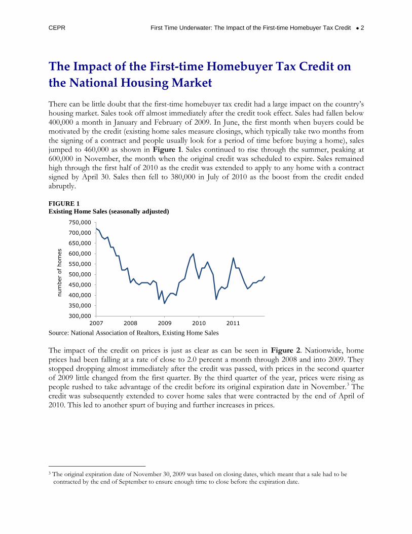
the National Housing Market There can be little doubt that the first-time homebuyer tax credit had a large impact on the country’s housing market. Sales took off almost immediately after the credit took effect. Sales had fallen below 400,000 a month in January and February of 2009. In June, the first month when buyers could be motivated by the credit (existing home sales measure closings, which typically take two months from the signing of a contract and people usually look for a period of time before buying a home), sales jumped to 460,000 as shown in Figure 1. Sales continued to rise through the summer, peaking at 600,000 in November, the month when the original credit was scheduled to expire. Sales remained high through the first half of 2010 as the credit was extended to apply to any home with a contract signed by April 30. Sales then fell to 380,000 in July of 2010 as the boost from the credit ended abruptly. FIGURE 1

Existing Home Sales (seasonally adjusted)

Source: National Association of Realtors, Existing Home Sales

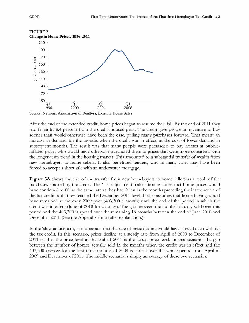
The impact of the credit on prices is just as clear as can be seen in Figure 2. Nationwide, home prices had been falling at a rate of close to 2.0 percent a month through 2008 and into 2009. They stopped dropping almost immediately after the credit was passed, with prices in the second quarter of 2009 little changed from the first quarter. By the third quarter of the year, prices were rising as people rushed to take advantage of the credit before its original expiration date in November.3 The credit was subsequently extended to cover home sales that were contracted by the end of April of 2010. This led to another spurt of buying and further increases in prices.

3 The original expiration date of November 30, 2009 was based on closing dates, which meant that a sale had to be

contracted by the end of September to ensure enough time to close before the expiration date.

300,000

350,000

400,000

450,000

500,000

550,000

600,000

650,000

700,000

750,000

2007 2008 2009 2010 2011

num

ber

of hom

es


FIGURE 2

Change in Home Prices, 1996-2011

Source: National Association of Realtors, Existing Home Sales

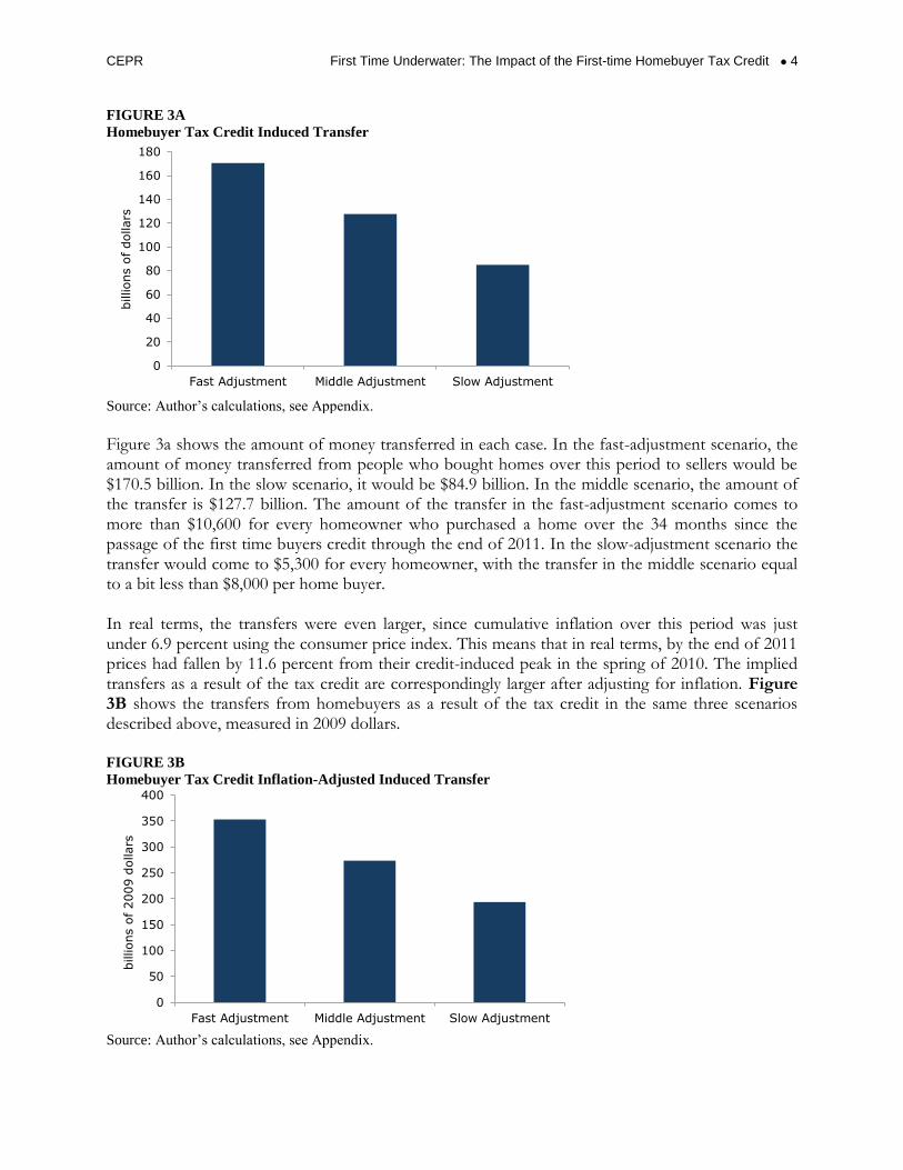
After the end of the extended credit, home prices began to resume their fall. By the end of 2011 they had fallen by 8.4 percent from the credit-induced peak. The credit gave people an incentive to buy sooner than would otherwise have been the case, pulling many purchases forward. That meant an increase in demand for the months when the credit was in effect, at the cost of lower demand in subsequent months. The result was that many people were persuaded to buy homes at bubble-inflated prices who would have otherwise purchased them at prices that were more consistent with the longer-term trend in the housing market. This amounted to a substantial transfer of wealth from new homebuyers to home sellers. It also benefitted lenders, who in many cases may have been forced to accept a short sale with an underwater mortgage. Figure 3A shows the size of the transfer from new homebuyers to home sellers as a result of the purchases spurred by the credit. The ‘fast adjustment’ calculation assumes that home prices would have continued to fall at the same rate as they had fallen in the months preceding the introduction of the tax credit, until they reached the December 2011 level. It also assumes that home buying would have remained at the early 2009 pace (403,300 a month) until the end of the period in which the credit was in effect (June of 2010 for closings). The gap between the number actually sold over this period and the 403,300 is spread over the remaining 18 months between the end of June 2010 and December 2011. (See the Appendix for a fuller explanation.) In the ‘slow adjustment,’ it is assumed that the rate of price decline would have slowed even without the tax credit. In this scenario, prices decline at a steady rate from April of 2009 to December of 2011 so that the price level at the end of 2011 is the actual price level. In this scenario, the gap between the number of homes actually sold in the months when the credit was in effect and the 403,300 average for the first three months of 2009 is spread over the whole period from April of 2009 and December of 2011. The middle scenario is simply an average of these two scenarios.

50

70

90

110

130

150

170

190

210

Q11996

Q12000

Q12004

Q12008

Q1 2

000 =

100


FIGURE 3A

Homebuyer Tax Credit Induced Transfer

Source: Author’s calculations, see Appendix.

Figure 3a shows the amount of money transferred in each case. In the fast-adjustment scenario, the amount of money transferred from people who bought homes over this period to sellers would be $170.5 billion. In the slow scenario, it would be $84.9 billion. In the middle scenario, the amount of the transfer is $127.7 billion. The amount of the transfer in the fast-adjustment scenario comes to more than $10,600 for every homeowner who purchased a home over the 34 months since the passage of the first time buyers credit through the end of 2011. In the slow-adjustment scenario the transfer would come to $5,300 for every homeowner, with the transfer in the middle scenario equal to a bit less than $8,000 per home buyer. In real terms, the transfers were even larger, since cumulative inflation over this period was just under 6.9 percent using the consumer price index. This means that in real terms, by the end of 2011 prices had fallen by 11.6 percent from their credit-induced peak in the spring of 2010. The implied transfers as a result of the tax credit are correspondingly larger after adjusting for inflation. Figure 3B shows the transfers from homebuyers as a result of the tax credit in the same three scenarios described above, measured in 2009 dollars. FIGURE 3B

Homebuyer Tax Credit Inflation-Adjusted Induced Transfer


0

20

40

60

80

100

120

140

160

180

Fast Adjustment Middle Adjustment Slow Adjustment

billions o

f dollars

0

50

100

150

200

250

300

350

400


billions o

f 2009 d

ollars


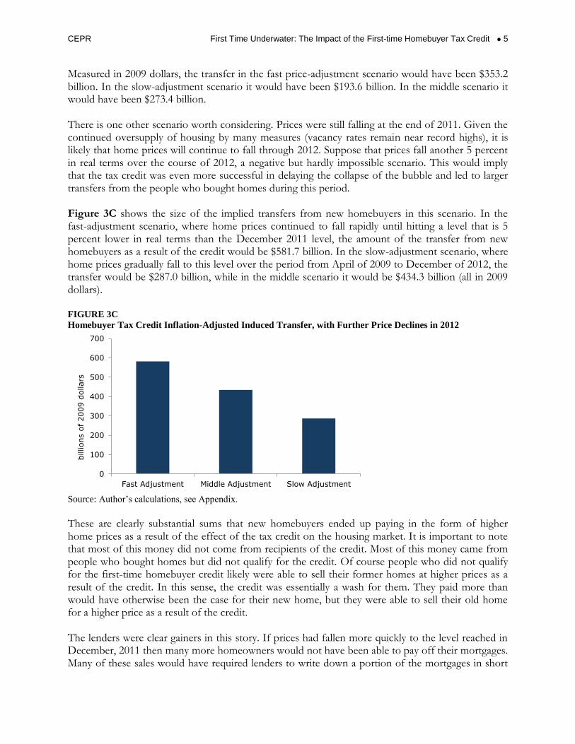
Measured in 2009 dollars, the transfer in the fast price-adjustment scenario would have been $353.2 billion. In the slow-adjustment scenario it would have been $193.6 billion. In the middle scenario it would have been $273.4 billion. There is one other scenario worth considering. Prices were still falling at the end of 2011. Given the continued oversupply of housing by many measures (vacancy rates remain near record highs), it is likely that home prices will continue to fall through 2012. Suppose that prices fall another 5 percent in real terms over the course of 2012, a negative but hardly impossible scenario. This would imply that the tax credit was even more successful in delaying the collapse of the bubble and led to larger transfers from the people who bought homes during this period. Figure 3C shows the size of the implied transfers from new homebuyers in this scenario. In the fast-adjustment scenario, where home prices continued to fall rapidly until hitting a level that is 5 percent lower in real terms than the December 2011 level, the amount of the transfer from new homebuyers as a result of the credit would be $581.7 billion. In the slow-adjustment scenario, where home prices gradually fall to this level over the period from April of 2009 to December of 2012, the transfer would be $287.0 billion, while in the middle scenario it would be $434.3 billion (all in 2009 dollars). FIGURE 3C

Homebuyer Tax Credit Inflation-Adjusted Induced Transfer, with Further Price Declines in 2012


These are clearly substantial sums that new homebuyers ended up paying in the form of higher home prices as a result of the effect of the tax credit on the housing market. It is important to note that most of this money did not come from recipients of the credit. Most of this money came from people who bought homes but did not qualify for the credit. Of course people who did not qualify for the first-time homebuyer credit likely were able to sell their former homes at higher prices as a result of the credit. In this sense, the credit was essentially a wash for them. They paid more than would have otherwise been the case for their new home, but they were able to sell their old home for a higher price as a result of the credit. The lenders were clear gainers in this story. If prices had fallen more quickly to the level reached in December, 2011 then many more homeowners would not have been able to pay off their mortgages. Many of these sales would have required lenders to write down a portion of the mortgages in short

0

100

200

300

400

500

600

700


billions o

f 2009 d

ollars


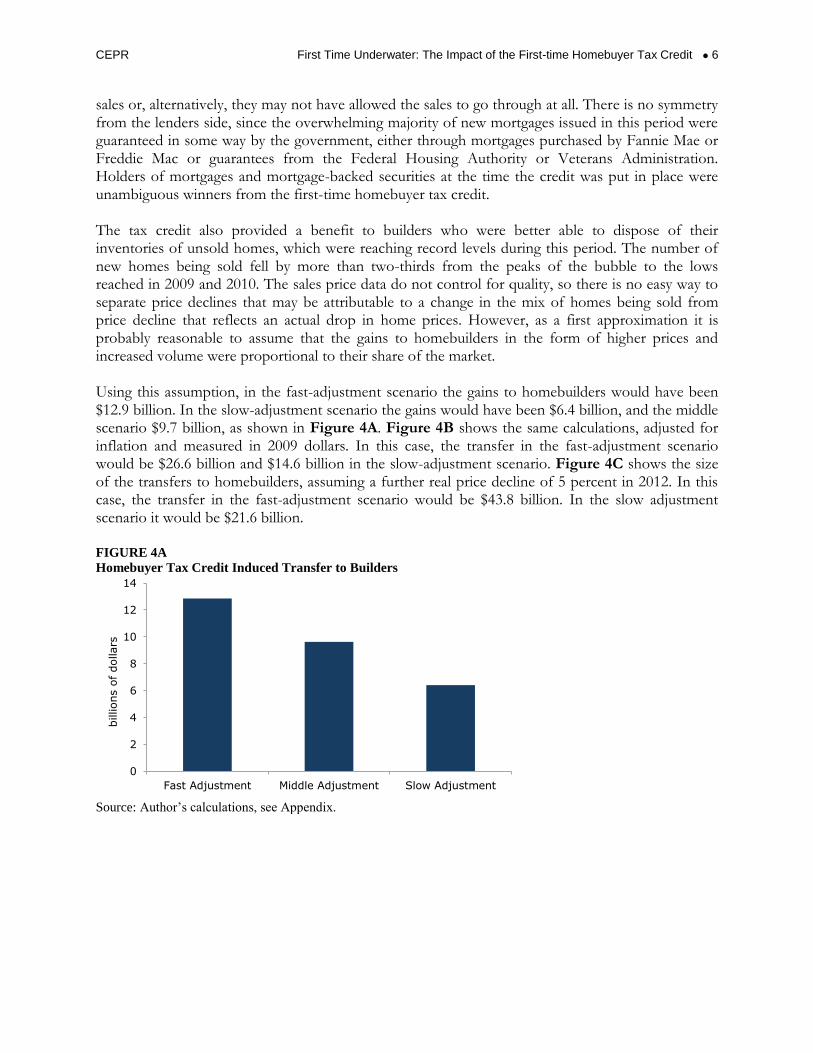
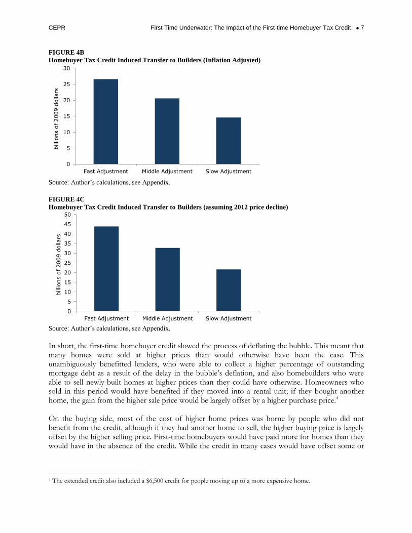
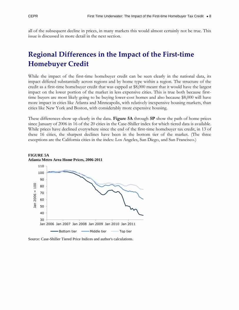
sales or, alternatively, they may not have allowed the sales to go through at all. There is no symmetry from the lenders side, since the overwhelming majority of new mortgages issued in this period were guaranteed in some way by the government, either through mortgages purchased by Fannie Mae or Freddie Mac or guarantees from the Federal Housing Authority or Veterans Administration. Holders of mortgages and mortgage-backed securities at the time the credit was put in place were unambiguous winners from the first-time homebuyer tax credit. The tax credit also provided a benefit to builders who were better able to dispose of their inventories of unsold homes, which were reaching record levels during this period. The number of new homes being sold fell by more than two-thirds from the peaks of the bubble to the lows reached in 2009 and 2010. The sales price data do not control for quality, so there is no easy way to separate price declines that may be attributable to a change in the mix of homes being sold from price decline that reflects an actual drop in home prices. However, as a first approximation it is probably reasonable to assume that the gains to homebuilders in the form of higher prices and increased volume were proportional to their share of the market. Using this assumption, in the fast-adjustment scenario the gains to homebuilders would have been $12.9 billion. In the slow-adjustment scenario the gains would have been $6.4 billion, and the middle scenario $9.7 billion, as shown in Figure 4A. Figure 4B shows the same calculations, adjusted for inflation and measured in 2009 dollars. In this case, the transfer in the fast-adjustment scenario would be $26.6 billion and $14.6 billion in the slow-adjustment scenario. Figure 4C shows the size of the transfers to homebuilders, assuming a further real price decline of 5 percent in 2012. In this case, the transfer in the fast-adjustment scenario would be $43.8 billion. In the slow adjustment scenario it would be $21.6 billion. FIGURE 4A

Homebuyer Tax Credit Induced Transfer to Builders


0

2

4

6

8

10

12

14


billions o

f dollars


FIGURE 4B

Homebuyer Tax Credit Induced Transfer to Builders (Inflation Adjusted)


FIGURE 4C

Homebuyer Tax Credit Induced Transfer to Builders (assuming 2012 price decline)


In short, the first-time homebuyer credit slowed the process of deflating the bubble. This meant that many homes were sold at higher prices than would otherwise have been the case. This unambiguously benefitted lenders, who were able to collect a higher percentage of outstanding mortgage debt as a result of the delay in the bubble’s deflation, and also homebuilders who were able to sell newly-built homes at higher prices than they could have otherwise. Homeowners who sold in this period would have benefited if they moved into a rental unit; if they bought another home, the gain from the higher sale price would be largely offset by a higher purchase price.4 On the buying side, most of the cost of higher home prices was borne by people who did not benefit from the credit, although if they had another home to sell, the higher buying price is largely offset by the higher selling price. First-time homebuyers would have paid more for homes than they would have in the absence of the credit. While the credit in many cases would have offset some or

4 The extended credit also included a $6,500 credit for people moving up to a more expensive home.

0

5

10

15

20

25

30


billions o

f 2009 d

ollars

0

5

10

15

20

25

30

35

40

45

50


billions o

f 2009 d

ollars


all of the subsequent decline in prices, in many markets this would almost certainly not be true. This issue is discussed in more detail in the next section.

Regional Differences in the Impact of the First-time

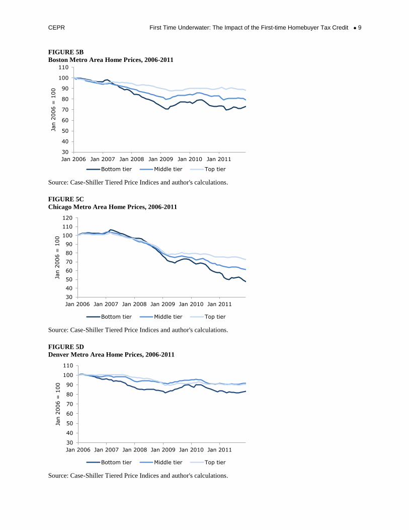
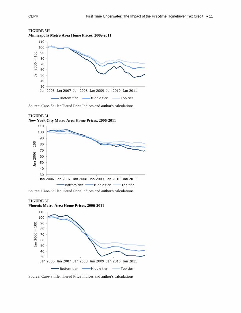
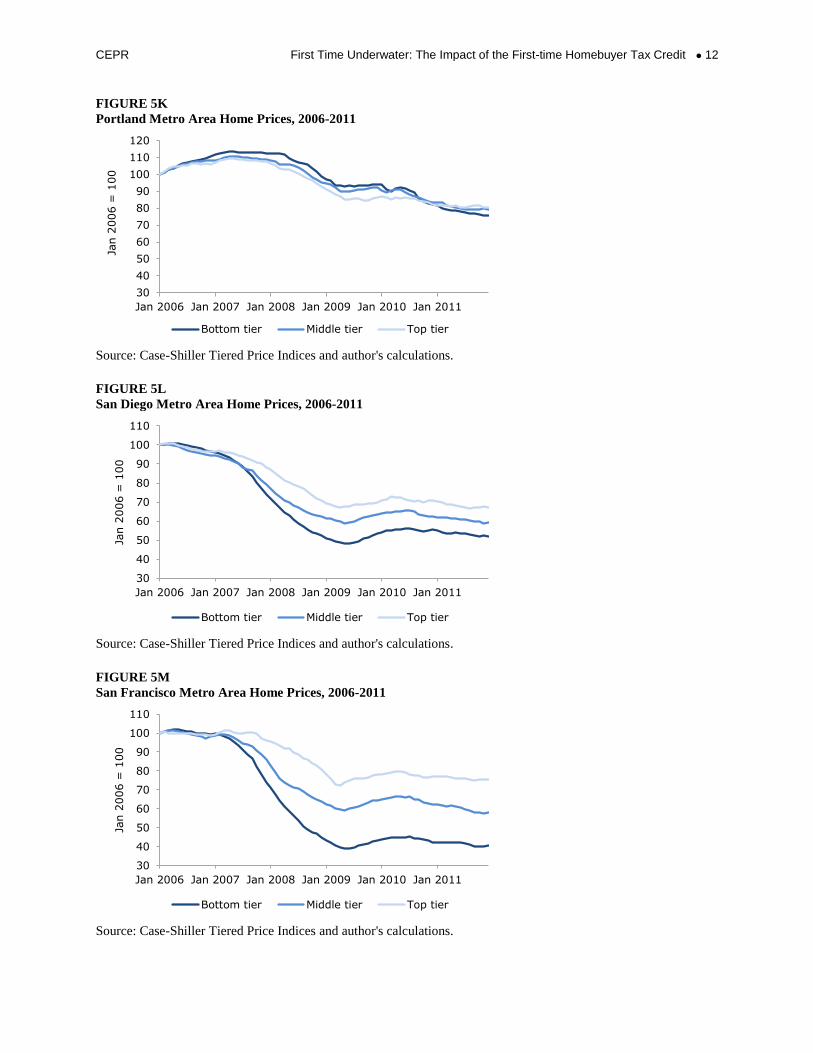
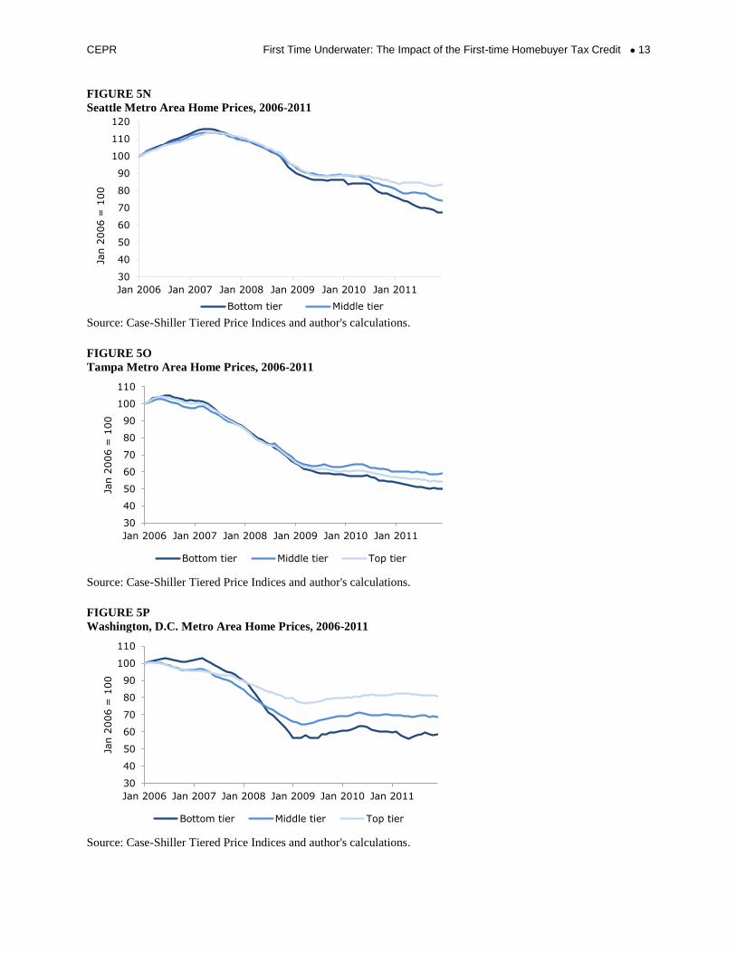
Homebuyer Credit While the impact of the first-time homebuyer credit can be seen clearly in the national data, its impact differed substantially across regions and by home type within a region. The structure of the credit as a first-time homebuyer credit that was capped at $8,000 meant that it would have the largest impact on the lower portion of the market in less expensive cities. This is true both because first-time buyers are most likely going to be buying lower-cost homes and also because $8,000 will have more impact in cities like Atlanta and Minneapolis, with relatively inexpensive housing markets, than cities like New York and Boston, with considerably more expensive housing. These differences show up clearly in the data. Figure 5A through 5P show the path of home prices since January of 2006 in 16 of the 20 cities in the Case-Shiller index for which tiered data is available. While prices have declined everywhere since the end of the first-time homebuyer tax credit, in 13 of these 16 cities, the sharpest declines have been in the bottom tier of the market. (The three exceptions are the California cities in the index: Los Angeles, San Diego, and San Francisco.) FIGURE 5A

Atlanta Metro Area Home Prices, 2006-2011

Source: Case-Shiller Tiered Price Indices and author's calculations.

30

40

50

60

70

80

90

100

110

Jan 2006 Jan 2007 Jan 2008 Jan 2009 Jan 2010 Jan 2011

Jan 2

006 =

100

Bottom tier Middle tier Top tier


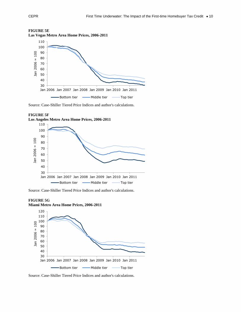
FIGURE 5B

Boston Metro Area Home Prices, 2006-2011


FIGURE 5C

Chicago Metro Area Home Prices, 2006-2011


FIGURE 5D

Denver Metro Area Home Prices, 2006-2011


30

40

50

60

70

80

90

100

110


Jan 2

006 =

100


30

40

50

60

70

80

90

100

110

120


Jan 2

006 =

100


30

40

50

60

70

80

90

100

110


Jan 2

006 =

100



FIGURE 5E

Las Vegas Metro Area Home Prices, 2006-2011


FIGURE 5F

Los Angeles Metro Area Home Prices, 2006-2011


FIGURE 5G

Miami Metro Area Home Prices, 2006-2011


30

40

50

60

70

80

90

100

110


Jan 2

006 =

100


30

40

50

60

70

80

90

100

110


Jan 2

006 =

100


30

40

50

60

70

80

90

100

110

120


Jan 2

006 =

100



FIGURE 5H

Minneapolis Metro Area Home Prices, 2006-2011


FIGURE 5I

New York City Metro Area Home Prices, 2006-2011


FIGURE 5J

Phoenix Metro Area Home Prices, 2006-2011


30

40

50

60

70

80

90

100

110


Jan 2

006 =

100


30

40

50

60

70

80

90

100

110


Jan 2

006 =

100


30

40

50

60

70

80

90

100

110


Jan 2

006 =

100



FIGURE 5K

Portland Metro Area Home Prices, 2006-2011


FIGURE 5L

San Diego Metro Area Home Prices, 2006-2011


FIGURE 5M

San Francisco Metro Area Home Prices, 2006-2011


30

40

50

60

70

80

90

100

110

120


Jan 2

006 =

100


30

40

50

60

70

80

90

100

110


Jan 2

006 =

100


30

40

50

60

70

80

90

100

110


Jan 2

006 =

100



FIGURE 5N

Seattle Metro Area Home Prices, 2006-2011


FIGURE 5O

Tampa Metro Area Home Prices, 2006-2011


FIGURE 5P

Washington, D.C. Metro Area Home Prices, 2006-2011


30

40

50

60

70

80

90

100

110

120


Jan 2

006 =

100

Bottom tier Middle tier

30

40

50

60

70

80

90

100

110


Jan 2

006 =

100


30

40

50

60

70

80

90

100

110


Jan 2

006 =

100



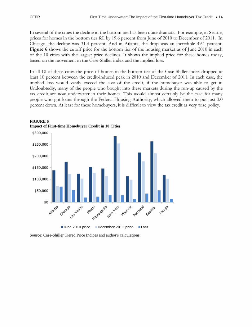
In several of the cities the decline in the bottom tier has been quite dramatic. For example, in Seattle, prices for homes in the bottom tier fell by 19.6 percent from June of 2010 to December of 2011. In Chicago, the decline was 31.4 percent. And in Atlanta, the drop was an incredible 49.1 percent. Figure 6 shows the cutoff price for the bottom tier of the housing market as of June 2010 in each of the 10 cities with the largest price declines. It shows the implied price for these homes today, based on the movement in the Case-Shiller index and the implied loss. In all 10 of these cities the price of homes in the bottom tier of the Case-Shiller index dropped at least 10 percent between the credit-induced peak in 2010 and December of 2011. In each case, the implied loss would vastly exceed the size of the credit, if the homebuyer was able to get it. Undoubtedly, many of the people who bought into these markets during the run-up caused by the tax credit are now underwater in their homes. This would almost certainly be the case for many people who got loans through the Federal Housing Authority, which allowed them to put just 3.0 percent down. At least for these homebuyers, it is difficult to view the tax credit as very wise policy. FIGURE 6

Impact of First-time Homebuyer Credit in 10 Cities


$0

$50,000

$100,000

$150,000

$200,000

$250,000

$300,000

June 2010 price December 2011 price Loss


Conclusion The fact that the first-time homebuyer credit would have the effect of luring millions of homebuyers into paying too much for a home should not have been a surprise. At the time the credit was put into effect, the housing bubble had not fully deflated, in the sense that home prices were still above their long-term trend. In this context, there was little reason to believe that a temporary tax credit could stabilize prices. The basic problem remained that home prices were above a level where supply and demand could be brought into balance. By pulling purchases forward the credit could only temporarily delay this adjustment process. The tax credit could redistribute the losses on housing, from the homeowners at the time the credit was passed and the holders of their mortgages to new homeowners and the holders of new mortgages, which was primarily the government. The size of this redistribution was in the hundreds of billions of dollars. It was remarkable that the Federal Reserve Board, the Treasury Department, the Council of Economic Advisers and other top economic officials managed to overlook the largest asset bubble in the history of the world as it was growing. It was even more remarkable that they continued to overlook it even as its collapse wrecked the economy and gave us the worst economic downturn since the Great Depression. If these officials had been paying attention, there would presumably have been more opposition to the first-time homebuyer tax credit.


Appendix Figure 3A – To construct the counterfactual set of prices and sales in order to calculate the amount of money transferred from sellers to buyers, the fast-adjustment assumed that home prices continued to fall at the same real rate they had been falling in the year prior to the passage of the first-time homebuyer tax credit (5.0 percent a quarter), until they reached the real level of December 2011. (The rate of price decline is taken from the Case-Shiller national index.) It assumed that the sales rate for all of 2009 would have remained at its level for the first four months of the year (403,300) in the absence of the credit until the end of the credit’s impact in June of 2010. The additional sales over this period (1,537,000 houmes) are then spread evenly over the subsequent 18 months from July 2010 until December of 2011. The revenue transferred is then the difference between revenue calculated using actual sales prices and quantities and these assumed counterfactuals summed over the period from June 2009 to June 2010. In the slow-adjustment scenario, it is assumed that prices would have adjusted at an even pace to their December 2011 level, falling at a real rate of 0.35 percent per month. This calculation assumes that in the absence of the credit the additional 1,537,000 in home sales calculated above would have been distributed evenly over the months from June of 2009 through December of 2011, with this number (49,600) being added to actual sales for the months after the end of the credit’s impact in 2010. In the months for which the credit was having an effect, this number was added to 403,300 baseline assumed in the fast decline scenario described above. The size of the revenue transfer was calculated in the same way described above. The middle scenario is a simple average of these two calculations. Figure 3B – The calculation in Figure 3B uses the consumer price index to express the totals in Figure 3A in 2009 dollars. Figure 3C – The fast-adjustment scenario assumes a counterfactual with the same rate of price decline as in Figure 1, except this rate of price decline continues until real prices hit a level that is 5 percent below their December 2011 level. The slow adjustment scenario assumes an even rate of price decline so that prices in December 2012 hit a real level that is 5.0 percent below the December 2011 level. The rate of home sales assumed in these counterfactuals is the same as described for Figure 1 above. The middle scenario is also calculated in the same way. Figures 4a, 4b, and 4c – These were constructed in the same way as Figures 3a, 3b, and 3c, with the only difference that data on new homes sales and prices were used.

Documents

First Time Underwater - CEPR