First LIGO search for gravitational wave bursts from cosmic (super)strings

First LIGO search for gravitational wave bursts from cosmic (super)strings

B. P. Abbott,17 R. Abbott,17 R. Adhikari,17 P. Ajith,2 B. Allen,2,60 G. Allen,35 R. S. Amin,21 S. B. Anderson,17

W.G. Anderson,60 M.A. Arain,47 M. Araya,17 H. Armandula,17 P. Armor,60 Y. Aso,17 S. Aston,46 P. Aufmuth,16

C. Aulbert,2 S. Babak,1 P. Baker,24 S. Ballmer,17 C. Barker,18 D. Barker,18 B. Barr,48 P. Barriga,59 L. Barsotti,20

M.A. Barton,17 I. Bartos,10 R. Bassiri,48 M. Bastarrika,48 B. Behnke,1 M. Benacquista,42 J. Betzwieser,17

P. T. Beyersdorf,31 I. A. Bilenko,25 G. Billingsley,17 R. Biswas,60 E. Black,17 J. K. Blackburn,17 L. Blackburn,20 D. Blair,59

B. Bland,18 T. P. Bodiya,20 L. Bogue,19 R. Bork,17 V. Boschi,17 S. Bose,61 P. R. Brady,60 V. B. Braginsky,25 J. E. Brau,53

D.O. Bridges,19 M. Brinkmann,2 A. F. Brooks,17 D. A. Brown,36 A. Brummit,30 G. Brunet,20 A. Bullington,35

A. Buonanno,49 O. Burmeister,2 R. L. Byer,35 L. Cadonati,50 J. B. Camp,26 J. Cannizzo,26 K. C. Cannon,17 J. Cao,20

L. Cardenas,17 S. Caride,51 G. Castaldi,56 S. Caudill,21 M. Cavaglia,39 C. Cepeda,17 T. Chalermsongsak,17 E. Chalkley,48

P. Charlton,9 S. Chatterji,17 S. Chelkowski,46 Y. Chen,1,6 N. Christensen,8 C. T. Y. Chung,38 D. Clark,35 J. Clark,7

J. H. Clayton,60 T. Cokelaer,7 C. N. Colacino,12 R. Conte,55 D. Cook,18 T. R. C. Corbitt,20 N. Cornish,24 D. Coward,59

D. C. Coyne,17 J. D. E. Creighton,60 T. D. Creighton,42 A.M. Cruise,46 R.M. Culter,46 A. Cumming,48 L. Cunningham,48

S. L. Danilishin,25 K. Danzmann,2,16 B. Daudert,17 G. Davies,7 E. J. Daw,40 D. DeBra,35 J. Degallaix,2 V. Dergachev,51

S. Desai,37 R. DeSalvo,17 S. Dhurandhar,15 M. Dıaz,42 A. Dietz,7 F. Donovan,20 K. L. Dooley,47 E. E. Doomes,34

R.W. P. Drever,5 J. Dueck,2 I. Duke,20 J.-C. Dumas,59 J. G. Dwyer,10 C. Echols,17 M. Edgar,48 A. Effler,18 P. Ehrens,17

E. Espinoza,17 T. Etzel,17 M. Evans,20 T. Evans,19 S. Fairhurst,7 Y. Faltas,47 Y. Fan,59 D. Fazi,17 H. Fehrmann,2 L. S. Finn,37

K. Flasch,60 S. Foley,20 C. Forrest,54 N. Fotopoulos,60 A. Franzen,16 M. Frede,2 M. Frei,41 Z. Frei,12 A. Freise,46 R. Frey,53

T. Fricke,19 P. Fritschel,20 V. V. Frolov,19 M. Fyffe,19 V. Galdi,56 J. A. Garofoli,36 I. Gholami,1 J. A. Giaime,21,19

S. Giampanis,2 K.D. Giardina,19 K. Goda,20 E. Goetz,51 L.M. Goggin,60 G. Gonzalez,21 M. L. Gorodetsky,25 S. Goßler,2

R. Gouaty,21 A. Grant,48 S. Gras,59 C. Gray,18 M. Gray,4 R. J. S. Greenhalgh,30 A.M. Gretarsson,11 F. Grimaldi,20

R. Grosso,42 H. Grote,2 S. Grunewald,1 M. Guenther,18 E. K. Gustafson,17 R. Gustafson,51 B. Hage,16 J.M. Hallam,46

D. Hammer,60 G.D. Hammond,48 C. Hanna,17 J. Hanson,19 J. Harms,52 G.M. Harry,20 I.W. Harry,7 E. D. Harstad,53

K. Haughian,48 K. Hayama,42 J. Heefner,17 I. S. Heng,48 A. Heptonstall,17 M. Hewitson,2 S. Hild,46 E. Hirose,36 D. Hoak,19

K.A. Hodge,17 K. Holt,19 D. J. Hosken,45 J. Hough,48 D. Hoyland,59 B. Hughey,20 S. H. Huttner,48 D. R. Ingram,18

T. Isogai,8 M. Ito,53 A. Ivanov,17 B. Johnson,18 W.W. Johnson,21 D. I. Jones,57 G. Jones,7 R. Jones,48 L. Ju,59 P. Kalmus,17

V. Kalogera,28 S. Kandhasamy,52 J. Kanner,49 D. Kasprzyk,46 E. Katsavounidis,20 K. Kawabe,18 S. Kawamura,27

F. Kawazoe,2 W. Kells,17 D. G. Keppel,17 A. Khalaidovski,2 F. Y. Khalili,25 R. Khan,10 E. Khazanov,14 P. King,17

J. S. Kissel,21 S. Klimenko,47 K. Kokeyama,27 V. Kondrashov,17 R. Kopparapu,37 S. Koranda,60 D. Kozak,17 B. Krishnan,1

R. Kumar,48 P. Kwee,16 P. K. Lam,4 M. Landry,18 B. Lantz,35 A. Lazzarini,17 H. Lei,42 M. Lei,17 N. Leindecker,35

I. Leonor,53 C. Li,6 H. Lin,47 P. E. Lindquist,17 T. B. Littenberg,24 N.A. Lockerbie,58 D. Lodhia,46 M. Longo,56

M. Lormand,19 P. Lu,35 M. Lubinski,18 A. Lucianetti,47 H. Luck,2,16 B. Machenschalk,1 M. MacInnis,20 M. Mageswaran,17

K. Mailand,17 I. Mandel,28 V. Mandic,52 S. Marka,10 Z. Marka,10 A. Markosyan,35 J. Markowitz,20 E. Maros,17

I.W. Martin,48 R.M. Martin,47 J. N. Marx,17 K. Mason,20 F. Matichard,21 L. Matone,10 R.A. Matzner,41 N. Mavalvala,20

R. McCarthy,18 D. E. McClelland,4 S. C. McGuire,34 M. McHugh,23 G. McIntyre,17 D. J. A. McKechan,7 K. McKenzie,4

M. Mehmet,2 A. Melatos,38 A. C. Melissinos,54 D. F. Menendez,37 G. Mendell,18 R. A. Mercer,60 S. Meshkov,17

C. Messenger,2 M. S. Meyer,19 J. Miller,48 J. Minelli,37 Y. Mino,6 V. P. Mitrofanov,25 G. Mitselmakher,47 R. Mittleman,20

O. Miyakawa,17 B. Moe,60 S. D. Mohanty,42 S. R. P. Mohapatra,50 G. Moreno,18 T. Morioka,27 K. Mors,2 K. Mossavi,2

C. MowLowry,4 G. Mueller,47 H. Muller-Ebhardt,2 D. Muhammad,19 S. Mukherjee,42 H. Mukhopadhyay,15 A. Mullavey,4

J. Munch,45 P. G. Murray,48 E. Myers,18 J. Myers,18 T. Nash,17 J. Nelson,48 G. Newton,48 A. Nishizawa,27 K. Numata,26

J. O’Dell,30 B. O’Reilly,19 R. O’Shaughnessy,37 E. Ochsner,49 G.H. Ogin,17 D. J. Ottaway,45 R. S. Ottens,47 H. Overmier,19

B. J. Owen,37 Y. Pan,49 C. Pankow,47 M.A. Papa,1,60 V. Parameshwaraiah,18 P. Patel,17 M. Pedraza,17 S. Penn,13

A. Perreca,46 V. Pierro,56 I.M. Pinto,56 M. Pitkin,48 H. J. Pletsch,2 M.V. Plissi,48 F. Postiglione,55 M. Principe,56 R. Prix,2

L. Prokhorov,25 O. Punken,2 V. Quetschke,47 F. J. Raab,18 D. S. Rabeling,4 H. Radkins,18 P. Raffai,12 Z. Raics,10 N. Rainer,2

M. Rakhmanov,42 V. Raymond,28 C.M. Reed,18 T. Reed,22 H. Rehbein,2 S. Reid,48 D.H. Reitze,47 R. Riesen,19 K. Riles,51

B. Rivera,18 P. Roberts,3 N.A. Robertson,17,48 C. Robinson,7 E. L. Robinson,1 S. Roddy,19 C. Rover,2 J. Rollins,10

J. D. Romano,42 J. H. Romie,19 S. Rowan,48 A. Rudiger,2 P. Russell,17 K. Ryan,18 S. Sakata,27 L. Sancho de la Jordana,44

V. Sandberg,18 V. Sannibale,17 L. Santamarıa,1 S. Saraf,32 P. Sarin,20 B. S. Sathyaprakash,7 S. Sato,27 M. Satterthwaite,4

P. R. Saulson,36 R. Savage,18 P. Savov,6 M. Scanlan,22 R. Schilling,2 R. Schnabel,2 R. Schofield,53 B. Schulz,2

B. F. Schutz,1,7 P. Schwinberg,18 J. Scott,48 S.M. Scott,4 A. C. Searle,17 B. Sears,17 F. Seifert,2 D. Sellers,19

PHYSICAL REVIEW D 80, 062002 (2009)

1550-7998=2009=80(6)=062002(11) 062002-1 � 2009 The American Physical Society

A. S. Sengupta,17 A. Sergeev,14 B. Shapiro,20 P. Shawhan,49 D.H. Shoemaker,20 A. Sibley,19 X. Siemens,60 D. Sigg,18

S. Sinha,35 A.M. Sintes,44 B. J. J. Slagmolen,4 J. Slutsky,21 J. R. Smith,36 M. R. Smith,17 N.D. Smith,20 K. Somiya,6

B. Sorazu,48 A. Stein,20 L. C. Stein,20 S. Steplewski,61 A. Stochino,17 R. Stone,42 K.A. Strain,48 S. Strigin,25 A. Stroeer,26

A. L. Stuver,19 T. Z. Summerscales,3 K.-X. Sun,35 M. Sung,21 P. J. Sutton,7 G. P. Szokoly,12 D. Talukder,61 L. Tang,42

D. B. Tanner,47 S. P. Tarabrin,25 J. R. Taylor,2 R. Taylor,17 J. Thacker,19 K.A. Thorne,19 K. S. Thorne,6 A. Thuring,16

K.V. Tokmakov,48 C. Torres,19 C. Torrie,17 G. Traylor,19 M. Trias,44 D. Ugolini,43 J. Ulmen,35 K. Urbanek,35

H. Vahlbruch,16 M. Vallisneri,6 C. Van Den Broeck,7 M.V. van der Sluys,28 A. A. van Veggel,48 S. Vass,17 R. Vaulin,60

A. Vecchio,46 J. Veitch,46 P. Veitch,45 C. Veltkamp,2 A. Villar,17 C. Vorvick,18 S. P. Vyachanin,25 S. J. Waldman,20

L. Wallace,17 R. L. Ward,17 A. Weidner,2 M. Weinert,2 A. J. Weinstein,17 R. Weiss,20 L. Wen,6,59 S. Wen,21 K. Wette,4

J. T. Whelan,1,29 S. E. Whitcomb,17 B. F. Whiting,47 C. Wilkinson,18 P. A. Willems,17 H. R. Williams,37 L. Williams,47

B. Willke,2,16 I. Wilmut,30 L. Winkelmann,2 W. Winkler,2 C. C. Wipf,20 A.G. Wiseman,60 G. Woan,48 R. Wooley,19

J. Worden,18 W. Wu,47 I. Yakushin,19 H. Yamamoto,17 Z. Yan,59 S. Yoshida,33 M. Zanolin,11 J. Zhang,51 L. Zhang,17

C. Zhao,59 N. Zotov,22 M. E. Zucker,20 H. zur Muhlen,16 J. Zweizig,17 and F. Robinet62

(The LIGO Scientific Collaboration)*

1Albert-Einstein-Institut, Max-Planck-Institut fur Gravitationsphysik, D-14476 Golm, Germany2Albert-Einstein-Institut, Max-Planck-Institut fur Gravitationsphysik, D-30167 Hannover, Germany

3Andrews University, Berrien Springs, Michigan 49104 USA4Australian National University, Canberra, 0200, Australia

5California Institute of Technology, Pasadena, California 91125, USA6Caltech-CaRT, Pasadena, California 91125, USA

7Cardiff University, Cardiff, CF24 3AA, United Kingdom8Carleton College, Northfield, Minnesota 55057, USA

9Charles Sturt University, Wagga Wagga, NSW 2678, Australia10Columbia University, New York, New York 10027, USA

11Embry-Riddle Aeronautical University, Prescott, Arizona 86301 USA12Eotvos University, ELTE 1053 Budapest, Hungary

13Hobart and William Smith Colleges, Geneva, New York 14456, USA14Institute of Applied Physics, Nizhny Novgorod, 603950, Russia

15Inter-University Center for Astronomy and Astrophysics, Pune-411007, India16Leibniz Universitat Hannover, D-30167 Hannover, Germany

17LIGO-California Institute of Technology, Pasadena, California 91125, USA18LIGO-Hanford Observatory, Richland, Washington 99352, USA

19LIGO-Livingston Observatory, Livingston, Louisiana 70754, USA20LIGO-Massachusetts Institute of Technology, Cambridge, Massachusetts 02139, USA

21Louisiana State University, Baton Rouge, Louisiana 70803, USA22Louisiana Tech University, Ruston, Louisiana 71272, USA23Loyola University, New Orleans, Louisiana 70118, USA

24Montana State University, Bozeman, Montana 59717, USA25Moscow State University, Moscow, 119992, Russia

26NASA/Goddard Space Flight Center, Greenbelt, Maryland 20771, USA27National Astronomical Observatory of Japan, Tokyo 181-8588, Japan

28Northwestern University, Evanston, Illinois 60208, USA29Rochester Institute of Technology, Rochester, New York 14623, USA

30Rutherford Appleton Laboratory, Harwell Science and Innovation Campus, Chilton, Didcot, Oxon OX11 0QX United Kingdom31San Jose State University, San Jose, California 95192, USA

32Sonoma State University, Rohnert Park, California 94928, USA33Southeastern Louisiana University, Hammond, Louisiana 70402, USA

34Southern University and A&M College, Baton Rouge, Louisiana 70813, USA35Stanford University, Stanford, California 94305, USA36Syracuse University, Syracuse, New York 13244, USA

37The Pennsylvania State University, University Park, Pennsylvania 16802, USA38The University of Melbourne, Parkville VIC 3010, Australia

39The University of Mississippi, University, Mississippi 38677, USA40The University of Sheffield, Sheffield S10 2TN, United Kingdom, USA

41The University of Texas at Austin, Austin, Texas 78712, USA42The University of Texas at Brownsville and Texas Southmost College, Brownsville, Texas 78520, USA

B. P. ABBOTT et al. PHYSICAL REVIEW D 80, 062002 (2009)

062002-2

43Trinity University, San Antonio, Texas 78212, USA44Universitat de les Illes Balears, E-07122 Palma de Mallorca, Spain

45University of Adelaide, Adelaide, SA 5005, Australia46University of Birmingham, Birmingham, B15 2TT, United Kingdom

47University of Florida, Gainesville, Florida 32611, USA48University of Glasgow, Glasgow, G12 8QQ, United Kingdom49University of Maryland, College Park, Maryland 20742 USA

50University of Massachusetts-Amherst, Amherst, Massachusetts 01003, USA51University of Michigan, Ann Arbor, Michigan 48109, USA

52University of Minnesota, Minneapolis, Minnesota 55455, USA53University of Oregon, Eugene, Oregon 97403, USA

54University of Rochester, Rochester, New York 14627, USA55University of Salerno, 84084 Fisciano (Salerno), Italy

56University of Sannio at Benevento, I-82100 Benevento, Italy57University of Southampton, Southampton, SO17 1BJ, United Kingdom

58University of Strathclyde, Glasgow, G1 1XQ, United Kingdom59University of Western Australia, Crawley, Washington 6009, Australia, USA

60University of Wisconsin-Milwaukee, Milwaukee, Wisconsin 53201, USA61Washington State University, Pullman, Washington 99164, USA

62Laboratoire de l’Accelerateur Lineaire, Univ Paris-Sud, CNRS/IN2P3, Orsay, France(Received 29 May 2009; published 23 September 2009)

We report on a matched-filter search for gravitational wave bursts from cosmic string cusps using LIGO

data from the fourth science run (S4) which took place in February and March 2005. No gravitational

waves were detected in 14.9 days of data from times when all three LIGO detectors were operating. We

interpret the result in terms of a frequentist upper limit on the rate of gravitational wave bursts and use the

limits on the rate to constrain the parameter space (string tension, reconnection probability, and loop sizes)

of cosmic string models. Many grand unified theory-scale models (with string tension G�=c2 � 10�6)

can be ruled out at 90% confidence for reconnection probabilities p � 10�3 if loop sizes are set by

gravitational back reaction.

DOI: 10.1103/PhysRevD.80.062002 PACS numbers: 11.27.+d, 11.25.�w, 98.80.Cq

I. INTRODUCTION

Cosmic strings are one-dimensional topological defectsthat can form during phase transitions in the early universe[1,2]. Topological defect formation is generic in grandunified theories (GUTs), and cosmic string productionspecifically is generic in supersymmetric GUTs [3]. Instring theory motivated cosmological models, cosmicstrings may also form (and are referred to as cosmic super-strings to differentiate them from strings formed in phasetransitions) [4–13]. There are important differences be-tween cosmic superstrings and field theoretic strings.When superstrings meet they reconnect with probabilityp that can be less than unity. This is partly due to the factthat fundamental strings interact probabilistically.Furthermore, these models have extra spatial dimensionsso that even though two strings may meet in 3 dimensions,they miss each other in the extra dimensions. These twoeffects result in values of p in the range 10�3–1 [9]. Inaddition, in string theory motivated cosmological models,more than one type of string may form.

Cosmic strings and superstrings may produce a varietyof astrophysical signatures including gamma ray bursts

[14], ultrahigh energy cosmic rays [15], magnetogenesis[16], microlensing, strong and weak lensing [17–21], radiobursts [22], effects on the cosmic 21 cm power spectrum[23], effects on the cosmic microwave background (CMB)at small angular scales [24,25], and effects on the CMBpolarization [26].Cosmic strings and superstrings can also produce power-

ful bursts of gravitational waves [27–31]. The most potentbursts are produced at regions of string called cusps whichacquire large Lorentz boosts. The formation of cusps oncosmic strings is generic, and cusp gravitational wave-forms are simple and robust [32,33]. The large mass perunit length of cosmic strings combined with the largeLorentz boost may result in signals detectable by Earth-based interferometric gravitational wave detectors such asLIGO [34] and Virgo [35]. Thus, gravitational waves mayprovide a powerful probe of early universe physics.The LIGO detector network is comprised of three laser

interferometers. Two of them are located at the Hanford,WA site: a four-kilometer arm instrument referred to as H1,and a two-kilometer arm instrument referred to as H2. Asecond four-kilometer interferometer located at theLivingston, LA site, is referred to as L1. LIGO’s fourthscience run (S4) took place between February 22, 2005 andMarch 23, 2005. The configuration of the LIGO instru-*http://www.ligo.org

FIRST LIGO SEARCH FOR GRAVITATIONAL WAVE . . . PHYSICAL REVIEW D 80, 062002 (2009)

062002-3

http://dx.doi.org/10.1103/PhysRevD.80.062002

ments during the fourth science run (S4) is described in[36]. The sensitivity of this run was significantly betterthan that of previous runs: at the low frequencies relevantto this search, close to a factor of 10 more sensitive than theprevious science run S3, though still about a factor of 2 lesssensitive than LIGO’s most recent science run (S5), whichwas at design sensitivity.

In this work, we report on the results of a matched-filtersearch for bursts from cosmic string cusps performed on14.9 days of S4 data. We implement the data analysismethods described in [31] using a simple triple coinci-dence scheme. No gravitational waves were detected, andwe interpret the result in terms of a frequentist upper limiton the rate using the loudest event technique [37]. We usethe upper limit on the rate to constrain the parameter spaceof cosmic strings models. The sensitivity of the LIGOinstruments during the S4 run does not allow us to placeconstraints as tight as the indirect bounds from big bangnucleosynthesis [38]. In the future, however, we expect oursensitivity to surpass these limits for large areas of cosmicstring model parameter space.

In Sec. II we discuss data selection, data analysis tech-niques, and describe the analysis pipeline. In Sec. III wedescribe the computation of the rate of accidental eventswe expect to survive the thresholds and consistency checksof the pipeline (the so-called background), and we compareit to the events that made it to the end of the pipeline in oursearch (the so-called foreground). In Sec. IV we show howwe estimate the sensitivity of the analysis using simulatedgravitational wave signals. We compute the efficiency ofour pipeline, the fraction of simulated signals that wedetect, as a function of the strength of the signals. InSec. V we show how to estimate the rate of burst eventswe expect, the effective rate, using the efficiency curvesand the cosmological rate of events. We show the con-straints our data place on the parameter space of cosmicstring models. We conclude in Sec. VI.

II. DATA ANALYSIS

A. Data selection and conditioning

All available S4 science data when all three instrumentswere operating (triple coincident data) were used exceptfor periods

(1) with overflows in the error signal digitizer,(2) when airplanes flew over the detector sites,(3) thirty seconds prior to loss of lock (loss of resonance

of the Fabry-Perot cavities in the arms) of anyinstrument,

(4) of excessive wind,(5) of excessive seismic activity, and(6) with calibration uncertainties larger than 10%.

The total time of triple coincident data available after thesecuts is 14.9 days. Calibration of the data used in thisanalysis was performed in the time domain [39]. Thedata were high-pass filtered near 30 Hz to remove unnec-

essary low frequency content and down-sampled from theoriginal LIGO sampling rate of 16384 to 4096 Hz.

B. Matched filters and templates

For each of the three LIGO instruments, we then per-formed a matched-filter search on this data for gravita-tional bursts from cosmic string cusps, i.e. linearlypolarized signals of the form [28]

hþðfÞ ¼ Bf�4=3�ðfh � fÞ�ðf� flÞ: (1)

The amplitude of the cusp waveform is B�G�L2=3=ðc3rÞ, where G is Newton’s constant, � is themass per unit length of the string, L is the size of the featureon the string that produces the cusp, and r is the distancebetween the cusp and the point of observation. In naturalunits G�=c2 can be thought of as the dimensionless massper unit length, or tension, of cosmic strings. For GUT-scale cosmic strings, for example, G�=c2 ¼ 10�6 [2]. Thesize L of the feature on the string that produces the cuspalso determines the low frequency cutoff fl. Since L isexpected to be cosmological, for example, the size of acosmic string loop, the low frequency cutoff of detectableradiation is determined by the low frequency behavior ofthe instruments: for the LIGO instruments by seismicnoise. The high frequency cutoff depends on the angle �between the line of sight and the direction of the cusp. It isgiven by fh � 2c=ð�3LÞ and can be arbitrarily large (up tothe inverse of the light crossing time of the width ofstrings).Following [31] for our templates, we take

�ðfÞ ¼ f�4=3�ðfh � fÞ�ðf� flÞ; (2)

so that hðfÞ ¼ A�ðfÞ. We can normalize our templates bydefining the detector-noise-weighted inner product [40] interms of the two frequency series xðfÞ and yðfÞ as

ðxjyÞ � 4<Z 1

0df

xðfÞy�ðfÞShðfÞ : (3)

Here, ShðfÞ is the single-sided spectral density defined byhnðfÞn�ðf0Þi ¼ 1

2�ðf� f0ÞShðfÞ, and nðfÞ is the Fourier

transform of the detector noise. We take the inner productof a template with itself to be �2 ¼ ð�j�Þ and define thenormalized template � � �=�, so that ð�j�Þ ¼ 1.The calibrated output of an interferometer can be written

as

sðtÞ ¼ nðtÞ þ hðtÞ; (4)

where nðtÞ is the instrumental noise, and hðtÞ ¼ FþhþðtÞthe gravitational wave signal. The antenna pattern responsefunction to þ-polarized gravitational waves, Fþ is a func-tion of the sky location of the cusp and the polarizationangle. The signal to noise ratio (SNR) is defined in terms ofthe inner product as � � ðsj�Þ. For the case of Gaussiannoise and in the absence of a signal, the SNR is a Gaussian


062002-4

variable with zero mean and unit variance. In the presenceof a signal of amplitude A, the signal to noise ratio is aGaussian random variable, with mean A� and unit vari-ance. Since the average SNR is h�i ¼ A�, for a particularrealization of the measured SNR �, we can identify asignal amplitude

A ¼ �=�; (5)

which has an average value hAi ¼ FþB.In our search, we set fl ¼ 50 Hz to be our low frequency

cutoff. Because of the low frequency behavior of ourinstruments, a negligible SNR would be gained by includ-ing frequencies lower than 50 Hz. We look for signals withhigh frequency cutoffs fh in the range 75–2048 Hz. Thesensitivity of the instruments is such that very little is lostby limiting the search to signals with high frequency cut-offs above 75 Hz and below 2048 Hz. The only templateparameter is the high frequency cutoff fh and the templatebank (the set of templates that determines the signals wesearch for) is constructed iteratively by computing theoverlap between adjacent templates [31]. The maximumfractional loss of signal to noise is set to 0.05 and alongwith the spectrum, determines the spacing between thehigh frequency cutoffs of the different templates. Thespectrum ShðfÞ is estimated using the median-meanmethod [41] which is fairly robust against nonstationaritiesin the data, including loud simulated signal injections.

C. Trigger generation

To produce our trigger data, we proceed as follows. Weapply the matched filter for each template and all possiblearrival times using fast Fourier transform convolution (asdescribed in [31]). This procedure results in a time seriesfor the SNR sampled at 4096 Hz for every template. Ineach of these time series, we search for clusters of valuesabove the threshold �th ¼ 4 which we identify as triggers.For each trigger we determine

(a) the SNR � of the trigger (the maximum SNR of thecluster),

(b) the peak time of the trigger (the location in time ofthe trigger SNR),

(c) the start time of the trigger (the first value abovethreshold in the cluster),

(d) the duration of the trigger (the length of the cluster),(e) the high frequency cutoff of the template, and(f) the amplitude of the trigger A, given by A ¼ �=�,

where � is the template normalization.When several templates result in triggers that occur withina time of 0.1 s, we select the trigger with the largest SNRwithin that time window.

We apply this procedure to the data sets of the threeLIGO interferometers to produce a list of triggers for eachinstrument.

D. Trigger consistency checks

To reduce the rate of events unassociated with gravita-tional waves (noise induced events), we demand that thepeak times of triggers in each instrument be coincident intime with triggers in the other two instruments. The timewindow used for H1-H2 events is 2 ms. This coincidencewindow allows for calibration uncertainties as well asshifts in the peak times of triggers induced by fluctuationsin the noise. For coincidence between events in either ofthe two Hanford instruments with events in the Livingstoninterferometer, a 12 ms coincidence window is used. Thisallows for the maximum light travel time between sites of10 ms along with calibration uncertainties and shifting ofthe peak location due to noise. We require strict triplecoincidence: in order for an event in one interferometerto survive, it must be coincident with events in the othertwo instruments and those two events must also becoincident.Additionally, we impose a symmetric consistency check

on the amplitudes of H1 and H2 coincident events [31]. Inparticular, for H1 events we demand that

jAH1 � AH2jAH1

<

��

�H1

þ �

�; (6)

along with an analogous requirement for H2 events. Here,� is the number of standard deviations of amplitude dif-ference we allow, and � is an additional fractional differ-ence that accounts for other sources of uncertainty such asthe calibration. We conservatively set � ¼ 3 and � ¼ 0:5.The purpose of this loose cut on the amplitude of events isto eliminate large SNR events seen in one instrument butnot in the other. These events are not due to gravitationalwaves but rather to instrumental glitches in the datastreams. It is worth pointing out that because each instru-ment has its own antenna response factor Fþ that dependson the orientation and direction of the gravitational wave,the H1-H2 amplitude consistency test cannot be applied toH1-L1 or H2-L1. Instruments that are not colocated mayhave different values of Fþ, and therefore the measuredamplitudes A could differ significantly.Both time coincidence and amplitude consistency

checks reduce the rate of events in each instrument fromabout 1 Hz to about 10 �Hz. To simplify the analysis in thefollowing, we only use the results and statistics for the H1events.

III. FOREGROUND AND BACKGROUND

To estimate the rate of accidental coincidences thatsurvive our consistency checks, the so-called background,we time shift the trigger sets relative to one another andlook for coincident events. We do not perform time shiftson the two Hanford trigger sets. Environmental disturban-ces are known to cause correlations between triggers inboth interferometers, and the effect of time shifting the two


062002-5

Hanford trigger sets would be to underestimate the back-ground. We therefore take the double coincident H1 andH2 triggers (which already satisfy the amplitude consis-tency check) and time shift them relative to the L1 triggerset. This amounts to treating the two Hanford instrumentsas a single trigger generator, on the same footing as L1 butwith a much smaller trigger rate. For each trigger in eachtime shift, we then demand the first consistency criterionbe satisfied, namely, that each Hanford trigger peak bewithin 12 ms of a Livingston trigger peak. We performed100 time shifts, with Livingston triggers shifted by ap-proximately 1.79 s, the total time shift ranging from�89:3 s to 89.3 s. The time shifts are large enough thatcoincident events cannot result from gravitational wavebursts from cosmic string cusps.

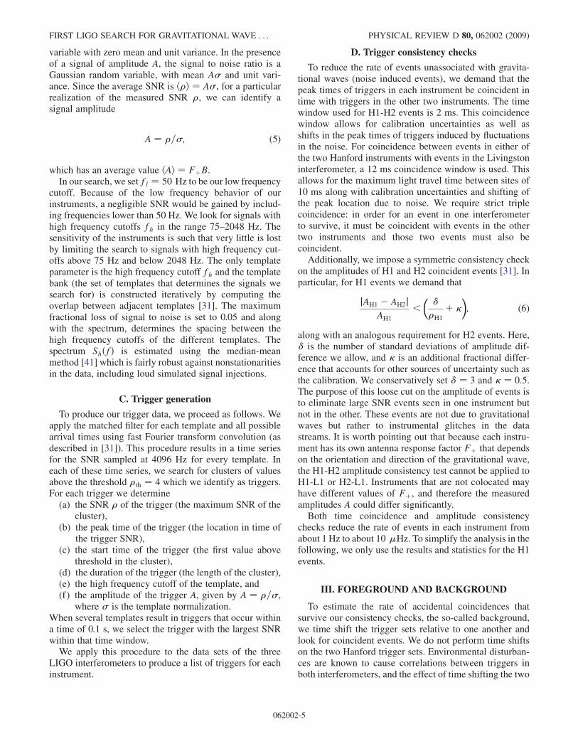
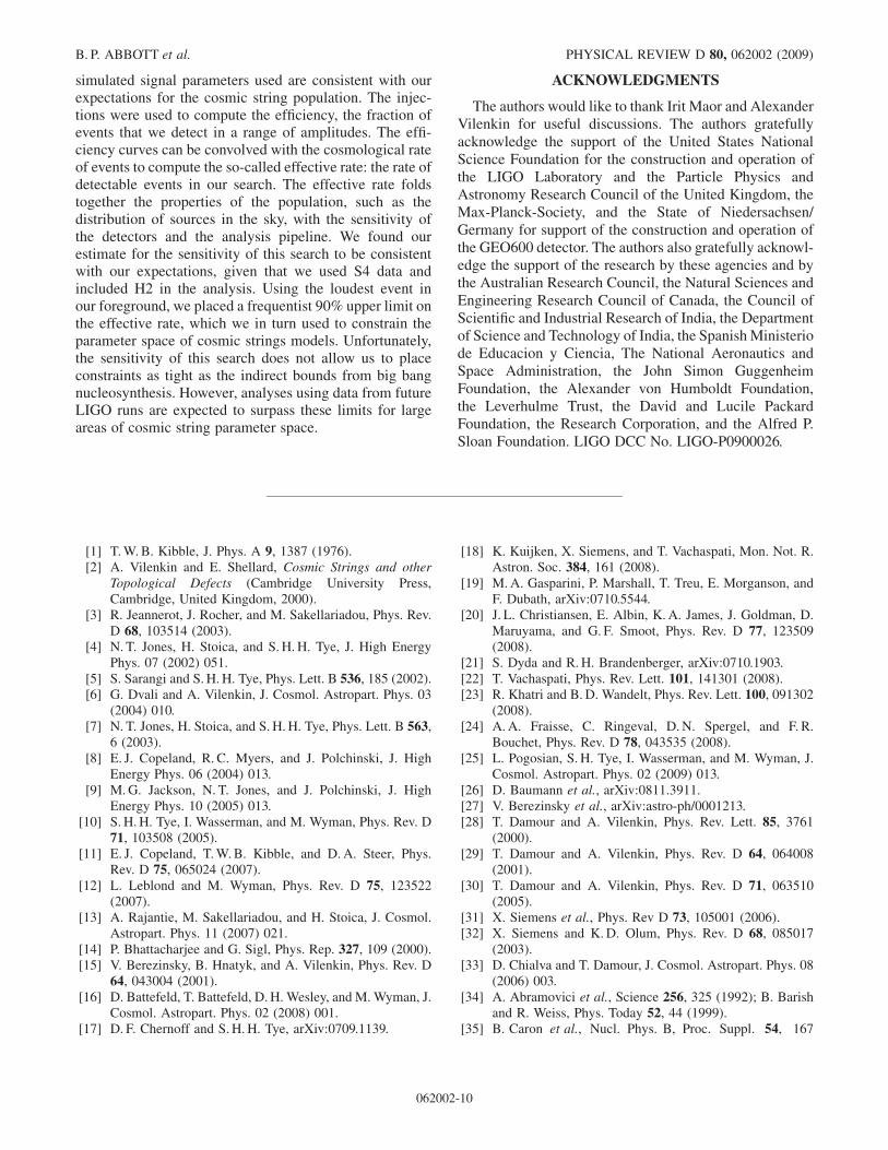
Figure 1 summarizes the results of this procedure for theH1 trigger set. We plot the cumulative rate of events forboth foreground (unshifted) events (filled circles), as wellas the average rate of events found in the time shifted data(stair steps) binned in amplitude. The shaded region cor-responds to 1-� uncertainties computed from the variationsin the number of events found in the time shifted data.

The loudest H1 event has an amplitude of AL ¼ 3:4�10�20 s�1=3. There are no foreground events which deviatesignificantly from the time slides, and a Kolmogorov-Smirnov test confirms that the foreground and backgrounddistributions are consistent at the 77% confidence level. Wetherefore conclude that no gravitational waves have beendetected in this search.

IV. EFFICIENCY

To determine our sensitivity and construct an upperlimit, we injected over 7400 simulated cusp signals intoour data set and performed a search identical to the onedescribed above.

The distribution of high frequency cutoffs fh for the

injected signals is dN / f�5=3h dfh, appropriate for the cusp

signals we are seeking [31]. The lowest high frequencycutoff injected is f� ¼ 75 Hz, coinciding with the lowesthigh frequency cutoff of our templates. The amplitudes are

distributed logarithmically between B ¼ 6� 10�21 s�1=3

and B ¼ 10�17 s�1=3 spanning the range of detectability.The sources are placed isotropically in the sky with suffi-cient separation in time so as not to unduly bias thespectrum estimate needed to perform the matched filter.An injection is found if its peak time lies between the

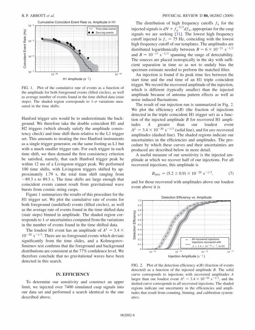
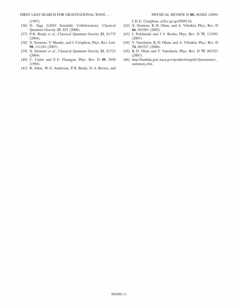
start time and the end time of an H1 triple coincidenttrigger. We record the recovered amplitude of the injection,which is different (typically smaller) than the injectedamplitude because of antenna pattern effects as well asnoise induced fluctuations.The result of our injection run is summarized in Fig. 2.

We plot the efficiency �ðBÞ (the fraction of injectionsdetected in the triple coincident H1 trigger set) as a func-tion of the injected amplitude B for recovered H1 ampli-tudes A greater than our loudest event

AL ¼ 3:4� 10�20 s�1=3 (solid line), and for any recoveredamplitudes (dashed line). The shaded regions indicate ouruncertainties in the efficiencies and amplitudes. The pro-cedure by which these curves and their uncertainties areproduced are described below in more detail.A useful measure of our sensitivity is the injected am-

plitude at which we recover half of our injections. For allrecovered injections, this amplitude is

B50% ¼ ð5:2� 0:9Þ � 10�20 s�1=3; (7)

and for those recovered with amplitudes above our loudestevent above it is

10− 20 10− 19

H1 Amplitude (s− 13 )

10− 7

10− 6

10− 5

10− 4C

oinc

iden

tEve

ntR

ate

(Hz)

Cumulative Coincident Event Rate vs. Amplitude in H1

Time-slide eventsZero-lag events

FIG. 1. Plot of the cumulative rate of events as a function ofthe amplitude for both foreground events (filled circles), as wellas average number of events found in the time shifted data (stairsteps). The shaded region corresponds to 1-� variations mea-sured in the time shifts.

10 20 10 19 10 18 10 17

Injection Amplitude (s13 )

0

0 1

0 2

0 3

0 4

0 5

0 6

0 7

0 8

0 9

1 0

Det

ectio

nE

ffici

ency

Detection Efficiency vs. Amplitude

All recovered injectionsInjections recovered with

3 4 10 20 s13 in H1

FIG. 2. Plot of the detection efficiency �ðBÞ (fraction of eventsdetected) as a function of the injected amplitude B. The solidcurve corresponds to injections with recovered amplitudes Alarger than our loudest event AL ¼ 3:4� 10�20 s�1=3, and thedashed curve corresponds to all recovered injections. The shadedregions indicate our uncertainty in the efficiencies and ampli-tudes that result from counting, binning, and calibration system-atics.


062002-6

BL50% ¼ ð1:1� 0:2Þ � 10�19 s�1=3: (8)

These numbers are consistent with our expectations. In[31], a sensitivity estimate was made for initial LIGO

BLIGO50% � 10�20 s�1=3. The current search is somewhat

less sensitive for two reasons. First, data from the S4 runis about a factor of 2 less sensitive than initial LIGO.Second, we demand coincidence with events in the H2interferometer which is about a factor of 2 less sensitivethan H1. Together, these account for a factor of about 4leaving only about a 30% discrepancy between the roughinitial LIGO sensitivity estimate made in [31] and Eq. (7).

As stated above, the software injections are generatedrandomly, with injected amplitudes that are uniformlydistributed in their logarithm. Individually, each injectionis either found or missed. To estimate the probability ofinjections with a given amplitude being recovered, we useda sliding window to count the number of software injec-tions that were made and recovered within an intervalaround that amplitude. The window used was Gaussianin the logarithm of the injected amplitudes. Choosingdifferent widths for the window will yield qualitativelyequivalent but quantitatively different efficiency curves.As pointed out above, a useful measure of our sensitivityis B50%, and we chose the width of the Gaussian window tominimize the uncertainty in B50%.

Three uncertainties are associated with the efficiencycurve. First, because at each point the value of the effi-ciency has been measured by counting a finite number ofinjections, there is an uncertainty in the efficiency attrib-utable to binomial counting fluctuations. Second, there isan uncertainty in the amplitude to which a measurement ofthe efficiency should be assigned, on account of it havingbeen found by counting injections spanning a range ofamplitudes. Finally, uncertainties in the calibration trans-late into an additional uncertainty in the amplitude, onaccount of the injections from which the efficiency wasmeasured having been done at amplitudes different fromwhat was intended. The calibration uncertainty we use is11%. This number results from the systematics in thecalibration models (5%) and our use of time domain cali-brated data (10%), which we combine in quadrature. Thecounting, amplitude range, and calibration uncertaintiesdescribed above are combined in quadrature to producethe shaded regions shown in Fig. 2.

V. PARAMETER SPACE OF COSMIC STRINGMODELS: CONSTRAINTS AND SENSITIVITY

For simplicity in this section, we will adopt units wherethe speed of light c ¼ 1. The parameter space of cosmicstring models we need to consider depends on whetherloops in the cosmic string network are short-lived (lifetimemuch smaller than a Hubble time) or long-lived (lifetimemuch larger than a Hubble time). This, in turn, depends onloop sizes at formation. If their size is given by the gravi-

tational back reaction scale [42,43], then to a good ap-proximation all loops have the same size at formation andthey are short-lived. In this case, their size at formation atcosmic time t can be approximated by l ¼ "�G�t, where" < 1 [30] is an unknown parameter that depends on thespectrum of perturbations on cosmic strings, and � is aconstant related to the lifetime of loops and is measured insimulations to be �� 50. Recent cosmic string networksimulations, however, suggest loops form at much largersizes given by the network dynamics [44,45]. If this is thecase, it has been shown [38] that the regions of parameterspace accessible to initial LIGO are already ruled out bypulsar timing experiments. So here, we will consider onlythe first possibility, that loop sizes are determined bygravitational back reaction and take the size of loops atformation to be l ¼ "�G�t. As mentioned, unlike fieldtheoretic cosmic strings, cosmic superstrings do not alwaysreconnect when they meet. Rather, they reconnect withprobability p � 1. The effect of the decreased reconnec-tion probability is to increase the density of strings by afactor inversely proportional to the reconnection probabil-ity [30].For a point in cosmic string parameter space (G�; "; p),

we can use the efficiency curves �ðBÞ to compute the rateof bursts we expect to observe in our instruments, whichwe will refer to as the effective rate . It is given by theintegral [31]

ðG�; "; pÞ ¼Z 1

0�ðBÞdRðB;G�; "; pÞ

dBdB; (9)

where B�G�l2=3=r is the optimally oriented amplitude(i.e. the amplitude of events excluding antenna patterneffects), �ðBÞ is the efficiency of detecting events at anamplitude B, and dRðB;G�; "; pÞ is the cosmological rateof events with amplitude in the interval B and Bþ dB. Wehave taken the size of the feature that produces the cusp tobe the size of the loop l.Since we are considering loops that are small when they

are formed, they are also short-lived, and at a given redshiftthey are all of essentially the same size. As a result, theamplitude of burst events from a given redshift is the same.In this case, rather than Eq. (9), it is easier to evaluate

ðG�; "; pÞ ¼Z 1

0�ðzÞdRðz;G�; "; pÞ

dzdz: (10)

Here, dRðzÞ is the rate of bursts originating at redshifts inthe interval between z and zþ dz. The rate is given byEq. (59) of [31]

dR

dz¼ H0

Ncðg2f�H�10 Þ�2=3

25=3p�G�’�14=3

t ðzÞ’VðzÞð1þ zÞ�5=3

��ð1� �mðz; f�; H�10 ’tðzÞÞ; (11)

where H0 is the present value of the Hubble parameter; Nc


062002-7

is the average number of cusps per loop oscillation; g2 is anignorance constant that absorbs the unknown fraction ofthe loop length that contributes to the cusp and otherfactors of Oð1Þ; f� is the lowest high frequency cutoff ofthe bursts we are interested in detecting; ¼ "�G� is the

loop formation size in units of the cosmic time; and �m ¼½g2ð1þ zÞf�l�1=3 is the maximum angle a cusp and theline of sight can subtend and still produce a burst with highfrequency cutoff f�. The � function removes events thatdo not have the form of Eq. (1). Two dimensionless cos-

mological functions enter the expression for the rate ofevents: ’tðzÞ which relates the cosmic time t and theredshift via t ¼ H�1

0 ’tðzÞ, and ’VðzÞ which determines

the proper volume element at a redshift z through dVðzÞ ¼H�3

0 ’VðzÞdz (see Appendix A of [31]). For details on the

derivation of this expression, see [28–31].The efficiency �ðzÞ is the fraction of events we detect

from a redshift z. We compute this quantity starting fromour measured efficiency as a function of the amplitude B,using Eq. (60) of [31]

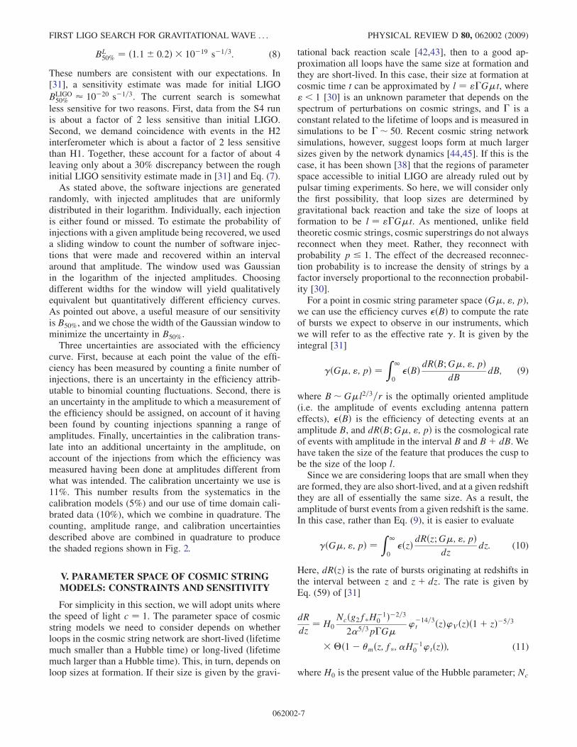
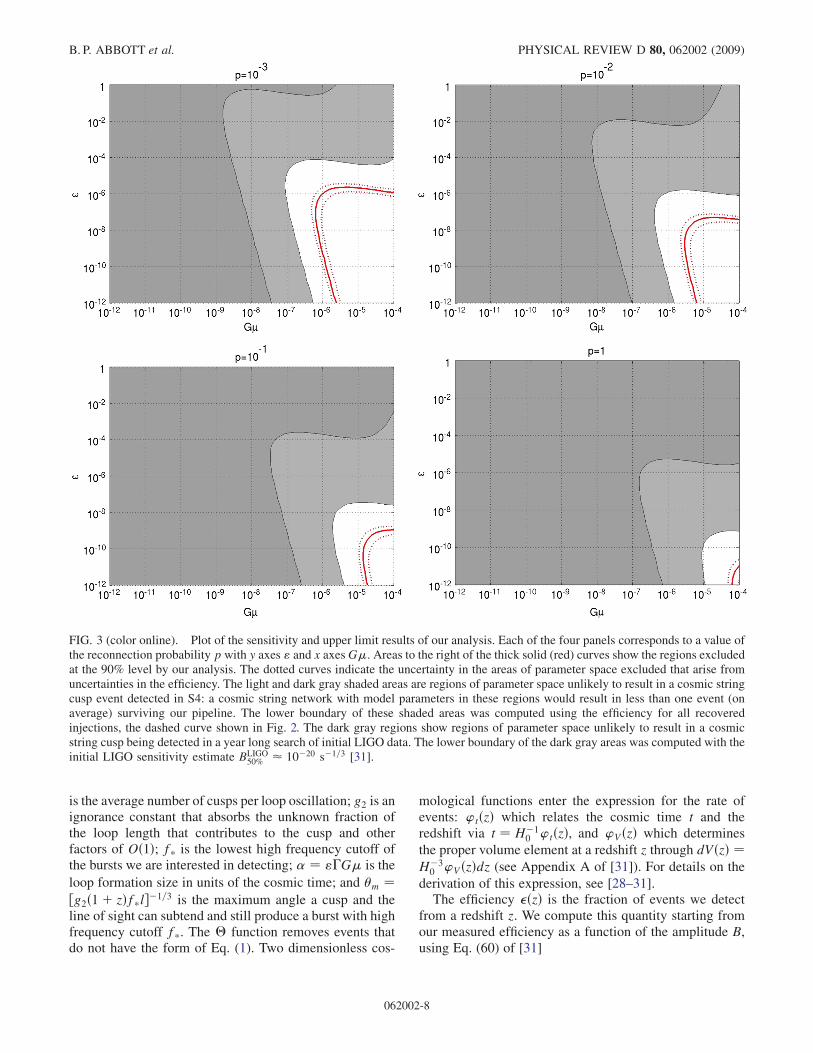
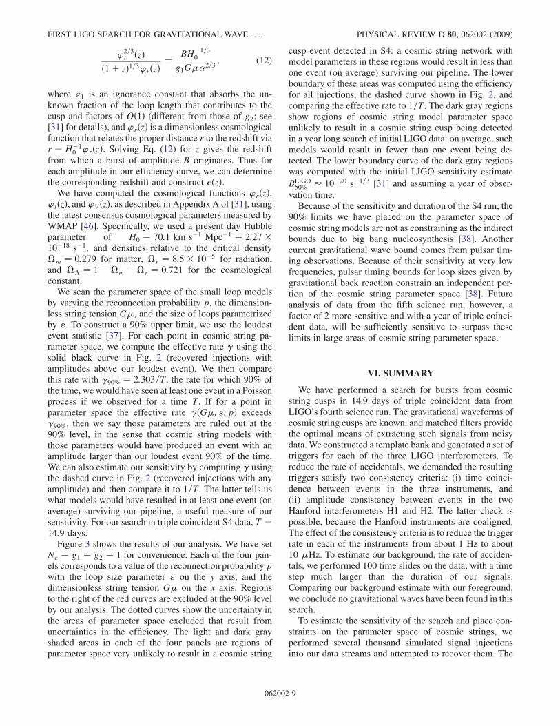
FIG. 3 (color online). Plot of the sensitivity and upper limit results of our analysis. Each of the four panels corresponds to a value ofthe reconnection probability p with y axes " and x axesG�. Areas to the right of the thick solid (red) curves show the regions excludedat the 90% level by our analysis. The dotted curves indicate the uncertainty in the areas of parameter space excluded that arise fromuncertainties in the efficiency. The light and dark gray shaded areas are regions of parameter space unlikely to result in a cosmic stringcusp event detected in S4: a cosmic string network with model parameters in these regions would result in less than one event (onaverage) surviving our pipeline. The lower boundary of these shaded areas was computed using the efficiency for all recoveredinjections, the dashed curve shown in Fig. 2. The dark gray regions show regions of parameter space unlikely to result in a cosmicstring cusp being detected in a year long search of initial LIGO data. The lower boundary of the dark gray areas was computed with theinitial LIGO sensitivity estimate BLIGO

50% � 10�20 s�1=3 [31].


062002-8

’2=3t ðzÞ

ð1þ zÞ1=3’rðzÞ¼ BH�1=3

0

g1G�2=3; (12)

where g1 is an ignorance constant that absorbs the un-known fraction of the loop length that contributes to thecusp and factors of Oð1Þ (different from those of g2; see[31] for details), and’rðzÞ is a dimensionless cosmologicalfunction that relates the proper distance r to the redshift viar ¼ H�1

0 ’rðzÞ. Solving Eq. (12) for z gives the redshift

from which a burst of amplitude B originates. Thus foreach amplitude in our efficiency curve, we can determinethe corresponding redshift and construct �ðzÞ.

We have computed the cosmological functions ’rðzÞ,’tðzÞ, and’VðzÞ, as described in Appendix A of [31], usingthe latest consensus cosmological parameters measured byWMAP [46]. Specifically, we used a present day Hubbleparameter of H0 ¼ 70:1 km s�1 Mpc�1 ¼ 2:27�10�18 s�1, and densities relative to the critical density�m ¼ 0:279 for matter, �r ¼ 8:5� 10�5 for radiation,and �� ¼ 1��m ��r ¼ 0:721 for the cosmologicalconstant.

We scan the parameter space of the small loop modelsby varying the reconnection probability p, the dimension-less string tension G�, and the size of loops parametrizedby ". To construct a 90% upper limit, we use the loudestevent statistic [37]. For each point in cosmic string pa-rameter space, we compute the effective rate using thesolid black curve in Fig. 2 (recovered injections withamplitudes above our loudest event). We then comparethis rate with 90% ¼ 2:303=T, the rate for which 90% ofthe time, wewould have seen at least one event in a Poissonprocess if we observed for a time T. If for a point inparameter space the effective rate ðG�; "; pÞ exceeds90%, then we say those parameters are ruled out at the90% level, in the sense that cosmic string models withthose parameters would have produced an event with anamplitude larger than our loudest event 90% of the time.We can also estimate our sensitivity by computing usingthe dashed curve in Fig. 2 (recovered injections with anyamplitude) and then compare it to 1=T. The latter tells uswhat models would have resulted in at least one event (onaverage) surviving our pipeline, a useful measure of oursensitivity. For our search in triple coincident S4 data, T ¼14:9 days.

Figure 3 shows the results of our analysis. We have setNc ¼ g1 ¼ g2 ¼ 1 for convenience. Each of the four pan-els corresponds to a value of the reconnection probability pwith the loop size parameter " on the y axis, and thedimensionless string tension G� on the x axis. Regionsto the right of the red curves are excluded at the 90% levelby our analysis. The dotted curves show the uncertainty inthe areas of parameter space excluded that result fromuncertainties in the efficiency. The light and dark grayshaded areas in each of the four panels are regions ofparameter space very unlikely to result in a cosmic string

cusp event detected in S4: a cosmic string network withmodel parameters in these regions would result in less thanone event (on average) surviving our pipeline. The lowerboundary of these areas was computed using the efficiencyfor all injections, the dashed curve shown in Fig. 2, andcomparing the effective rate to 1=T. The dark gray regionsshow regions of cosmic string model parameter spaceunlikely to result in a cosmic string cusp being detectedin a year long search of initial LIGO data: on average, suchmodels would result in fewer than one event being de-tected. The lower boundary curve of the dark gray regionswas computed with the initial LIGO sensitivity estimate

BLIGO50% � 10�20 s�1=3 [31] and assuming a year of obser-

vation time.Because of the sensitivity and duration of the S4 run, the

90% limits we have placed on the parameter space ofcosmic string models are not as constraining as the indirectbounds due to big bang nucleosynthesis [38]. Anothercurrent gravitational wave bound comes from pulsar tim-ing observations. Because of their sensitivity at very lowfrequencies, pulsar timing bounds for loop sizes given bygravitational back reaction constrain an independent por-tion of the cosmic string parameter space [38]. Futureanalysis of data from the fifth science run, however, afactor of 2 more sensitive and with a year of triple coinci-dent data, will be sufficiently sensitive to surpass theselimits in large areas of cosmic string parameter space.

VI. SUMMARY

We have performed a search for bursts from cosmicstring cusps in 14.9 days of triple coincident data fromLIGO’s fourth science run. The gravitational waveforms ofcosmic string cusps are known, and matched filters providethe optimal means of extracting such signals from noisydata. We constructed a template bank and generated a set oftriggers for each of the three LIGO interferometers. Toreduce the rate of accidentals, we demanded the resultingtriggers satisfy two consistency criteria: (i) time coinci-dence between events in the three instruments, and(ii) amplitude consistency between events in the twoHanford interferometers H1 and H2. The latter check ispossible, because the Hanford instruments are coaligned.The effect of the consistency criteria is to reduce the triggerrate in each of the instruments from about 1 Hz to about10 �Hz. To estimate our background, the rate of acciden-tals, we performed 100 time slides on the data, with a timestep much larger than the duration of our signals.Comparing our background estimate with our foreground,we conclude no gravitational waves have been found in thissearch.To estimate the sensitivity of the search and place con-

straints on the parameter space of cosmic strings, weperformed several thousand simulated signal injectionsinto our data streams and attempted to recover them. The


062002-9

simulated signal parameters used are consistent with ourexpectations for the cosmic string population. The injec-tions were used to compute the efficiency, the fraction ofevents that we detect in a range of amplitudes. The effi-ciency curves can be convolved with the cosmological rateof events to compute the so-called effective rate: the rate ofdetectable events in our search. The effective rate foldstogether the properties of the population, such as thedistribution of sources in the sky, with the sensitivity ofthe detectors and the analysis pipeline. We found ourestimate for the sensitivity of this search to be consistentwith our expectations, given that we used S4 data andincluded H2 in the analysis. Using the loudest event inour foreground, we placed a frequentist 90% upper limit onthe effective rate, which we in turn used to constrain theparameter space of cosmic strings models. Unfortunately,the sensitivity of this search does not allow us to placeconstraints as tight as the indirect bounds from big bangnucleosynthesis. However, analyses using data from futureLIGO runs are expected to surpass these limits for largeareas of cosmic string parameter space.

ACKNOWLEDGMENTS

The authors would like to thank Irit Maor and AlexanderVilenkin for useful discussions. The authors gratefullyacknowledge the support of the United States NationalScience Foundation for the construction and operation ofthe LIGO Laboratory and the Particle Physics andAstronomy Research Council of the United Kingdom, theMax-Planck-Society, and the State of Niedersachsen/Germany for support of the construction and operation ofthe GEO600 detector. The authors also gratefully acknowl-edge the support of the research by these agencies and bythe Australian Research Council, the Natural Sciences andEngineering Research Council of Canada, the Council ofScientific and Industrial Research of India, the Departmentof Science and Technology of India, the Spanish Ministeriode Educacion y Ciencia, The National Aeronautics andSpace Administration, the John Simon GuggenheimFoundation, the Alexander von Humboldt Foundation,the Leverhulme Trust, the David and Lucile PackardFoundation, the Research Corporation, and the Alfred P.Sloan Foundation. LIGO DCC No. LIGO-P0900026.

[1] T.W. B. Kibble, J. Phys. A 9, 1387 (1976).[2] A. Vilenkin and E. Shellard, Cosmic Strings and other

Topological Defects (Cambridge University Press,Cambridge, United Kingdom, 2000).

[3] R. Jeannerot, J. Rocher, and M. Sakellariadou, Phys. Rev.D 68, 103514 (2003).

[4] N. T. Jones, H. Stoica, and S.H. H. Tye, J. High EnergyPhys. 07 (2002) 051.

[5] S. Sarangi and S.H. H. Tye, Phys. Lett. B 536, 185 (2002).[6] G. Dvali and A. Vilenkin, J. Cosmol. Astropart. Phys. 03

(2004) 010.[7] N. T. Jones, H. Stoica, and S. H.H. Tye, Phys. Lett. B 563,

6 (2003).[8] E. J. Copeland, R. C. Myers, and J. Polchinski, J. High

Energy Phys. 06 (2004) 013.[9] M.G. Jackson, N. T. Jones, and J. Polchinski, J. High

Energy Phys. 10 (2005) 013.[10] S. H.H. Tye, I. Wasserman, and M. Wyman, Phys. Rev. D

71, 103508 (2005).[11] E. J. Copeland, T.W.B. Kibble, and D.A. Steer, Phys.

Rev. D 75, 065024 (2007).[12] L. Leblond and M. Wyman, Phys. Rev. D 75, 123522

(2007).[13] A. Rajantie, M. Sakellariadou, and H. Stoica, J. Cosmol.

Astropart. Phys. 11 (2007) 021.[14] P. Bhattacharjee and G. Sigl, Phys. Rep. 327, 109 (2000).[15] V. Berezinsky, B. Hnatyk, and A. Vilenkin, Phys. Rev. D

64, 043004 (2001).[16] D. Battefeld, T. Battefeld, D.H. Wesley, and M. Wyman, J.

Cosmol. Astropart. Phys. 02 (2008) 001.[17] D. F. Chernoff and S. H.H. Tye, arXiv:0709.1139.

[18] K. Kuijken, X. Siemens, and T. Vachaspati, Mon. Not. R.Astron. Soc. 384, 161 (2008).

[19] M.A. Gasparini, P. Marshall, T. Treu, E. Morganson, andF. Dubath, arXiv:0710.5544.

[20] J. L. Christiansen, E. Albin, K.A. James, J. Goldman, D.Maruyama, and G. F. Smoot, Phys. Rev. D 77, 123509(2008).

[21] S. Dyda and R.H. Brandenberger, arXiv:0710.1903.[22] T. Vachaspati, Phys. Rev. Lett. 101, 141301 (2008).[23] R. Khatri and B.D. Wandelt, Phys. Rev. Lett. 100, 091302

(2008).[24] A. A. Fraisse, C. Ringeval, D.N. Spergel, and F. R.

Bouchet, Phys. Rev. D 78, 043535 (2008).[25] L. Pogosian, S. H. Tye, I. Wasserman, and M. Wyman, J.

Cosmol. Astropart. Phys. 02 (2009) 013.[26] D. Baumann et al., arXiv:0811.3911.[27] V. Berezinsky et al., arXiv:astro-ph/0001213.[28] T. Damour and A. Vilenkin, Phys. Rev. Lett. 85, 3761

(2000).[29] T. Damour and A. Vilenkin, Phys. Rev. D 64, 064008

(2001).[30] T. Damour and A. Vilenkin, Phys. Rev. D 71, 063510

(2005).[31] X. Siemens et al., Phys. Rev D 73, 105001 (2006).[32] X. Siemens and K.D. Olum, Phys. Rev. D 68, 085017

(2003).[33] D. Chialva and T. Damour, J. Cosmol. Astropart. Phys. 08

(2006) 003.[34] A. Abramovici et al., Science 256, 325 (1992); B. Barish

and R. Weiss, Phys. Today 52, 44 (1999).[35] B. Caron et al., Nucl. Phys. B, Proc. Suppl. 54, 167


062002-10

(1997).[36] D. Sigg (LIGO Scientific Collaboration), Classical

Quantum Gravity 23, S51 (2006).[37] P. R. Brady et al., Classical Quantum Gravity 21, S1775

(2004).[38] X. Siemens, V. Mandic, and J. Creighton, Phys. Rev. Lett.

98, 111101 (2007).[39] X. Siemens et al., Classical Quantum Gravity 21, S1723

(2004).[40] C. Cutler and E. E. Flanagan, Phys. Rev. D 49, 2658

(1994).[41] B. Allen, W.G. Anderson, P. R. Brady, D. A. Brown, and

J. D. E. Creighton, arXiv:gr-qc/0509116.[42] X. Siemens, K. D. Olum, and A. Vilenkin, Phys. Rev. D

66, 043501 (2002).[43] J. Polchinski and J. V. Rocha, Phys. Rev. D 75, 123503

(2007).[44] V. Vanchurin, K.D. Olum, and A. Vilenkin, Phys. Rev. D

74, 063527 (2006).[45] K. D. Olum and V. Vanchurin, Phys. Rev. D 75, 063521

(2007).[46] http://lambda.gsfc.nasa.gov/product/map/dr3/parameters_

summary.cfm.


062002-11

Documents

First LIGO search for gravitational wave bursts from cosmic (super)strings