Embed Size (px)
Citation preview

Firm Selection and Corporate Cash Holdings
Juliane Begenau Berardino Palazzo
Working Paper 16-130

Working Paper 16-130
Copyright © 2016, 2017 by Juliane Begenau and Berardino Palazzo
Working papers are in draft form. This working paper is distributed for purposes of comment and discussion only. It may not be reproduced without permission of the copyright holder. Copies of working papers are available from the author.
Firm Selection and Corporate Cash Holdings
Juliane Begenau Harvard Business School
Berardino Palazzo Boston University
Firm Selection and Corporate Cash Holdings∗
Juliane Begenau Berardino PalazzoHarvard University & NBER Boston University
February 2017
Abstract
Among stock market entrants, more firms over time are R&D–intensive with initially
lower profitability but higher growth potential. This sample-selection effect determines
the secular trend in U.S. public firms’ cash holdings. A stylized firm industry model
allows us to analyze two competing changes to the selection mechanism: a change in
industry composition and a shift toward less profitable R&D–firms. The latter is key
to generating higher cash ratios at IPO, necessary for the secular increase, whereas the
former mechanism amplifies this effect. The data confirm the prominent role played
by selection, and corroborate the model’s predictions.
∗ We are particularly grateful to Joan Farre-Mensa for comments and suggestions and Young Min Kimfor excellent research assistance. We are also grateful to Rajesh Aggarwal, Rui Albuquerque, Andrea Buffa,Gian Luca Clementi, Marco Da Rin, Fritz Foley, Ambrus Kecskes, Pablo Kurlat, Evgeny Lyandres, SebastienMichenaud, Stefano Sacchetto, Martin Schmalz, Ken Singleton, Viktoriya Staneva, Anna-Leigh Stone, andToni Whited as well as seminar attendants at Boston University, Harvard University, IDC Summer Con-ference, SED meeting in Warsaw, Tepper-LAEF Conference on “Advances in Macro-Finance,” Christmasmeeting at LMU, Utah Winter Finance Conference, Midwest Finance Association Conference, SUNY atStony Brook, World Finance Conference, Federal Reserve Board, D’Amore-McKim School of Business, SimonSchool of Business, Carlson School of Management Finance Department Junior Conference, and DriehausCollege of Business for their comments and suggestions. All remaining errors are our own responsibility.Correspondence: Juliane Begenau ([email protected]) and Berardino Palazzo ([email protected]).
1 Introduction
The average U.S. public firm has changed its characteristics over the last 35 years. The
disappearance of dividends (Fama and French (2001)), the decline in profitability (Fama
and French (2004)), the increase in cash holdings (Bates et al. (2009)) and firm-specific
risk measures (Davis et al. (2007) and Brown and Kapadia (2007)) are phenomena of this
period. A change in the behavior of the average public firm could be caused by a change in
the behavior of incumbent firms as well as by the selection of a different type of firm into
the stock market that gradually replaces incumbent firms over time.
This paper studies and quantifies the role of sample selection for the secular increase
in the average cash–to–assets ratio of U.S. public companies over the last 35 years.1 The
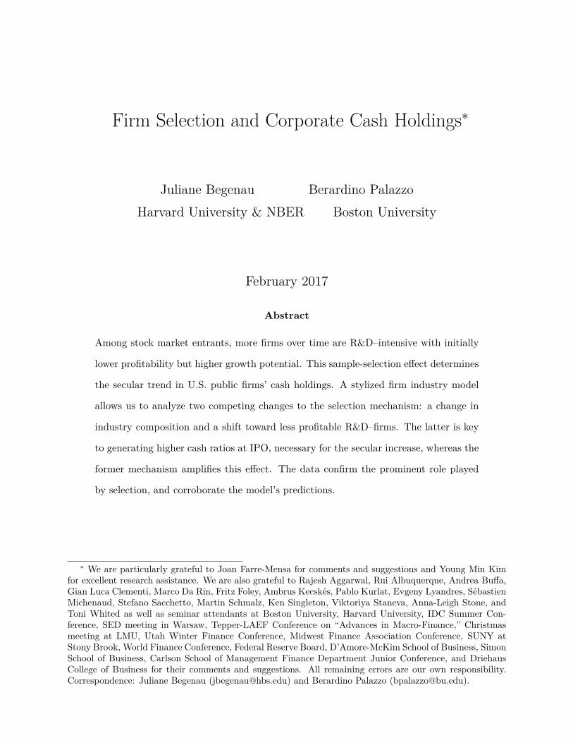
following facts motivate our research. Since the beginning of the 1980s, firms went public
with progressively higher cash–to–assets ratios, but they reduced their cash ratios gradually
afterward (see Figure 1).2 This feature of the data is indicative of a sample-selection mecha-
nism, namely, a change in the conditions that determine which firms choose to enter the stock
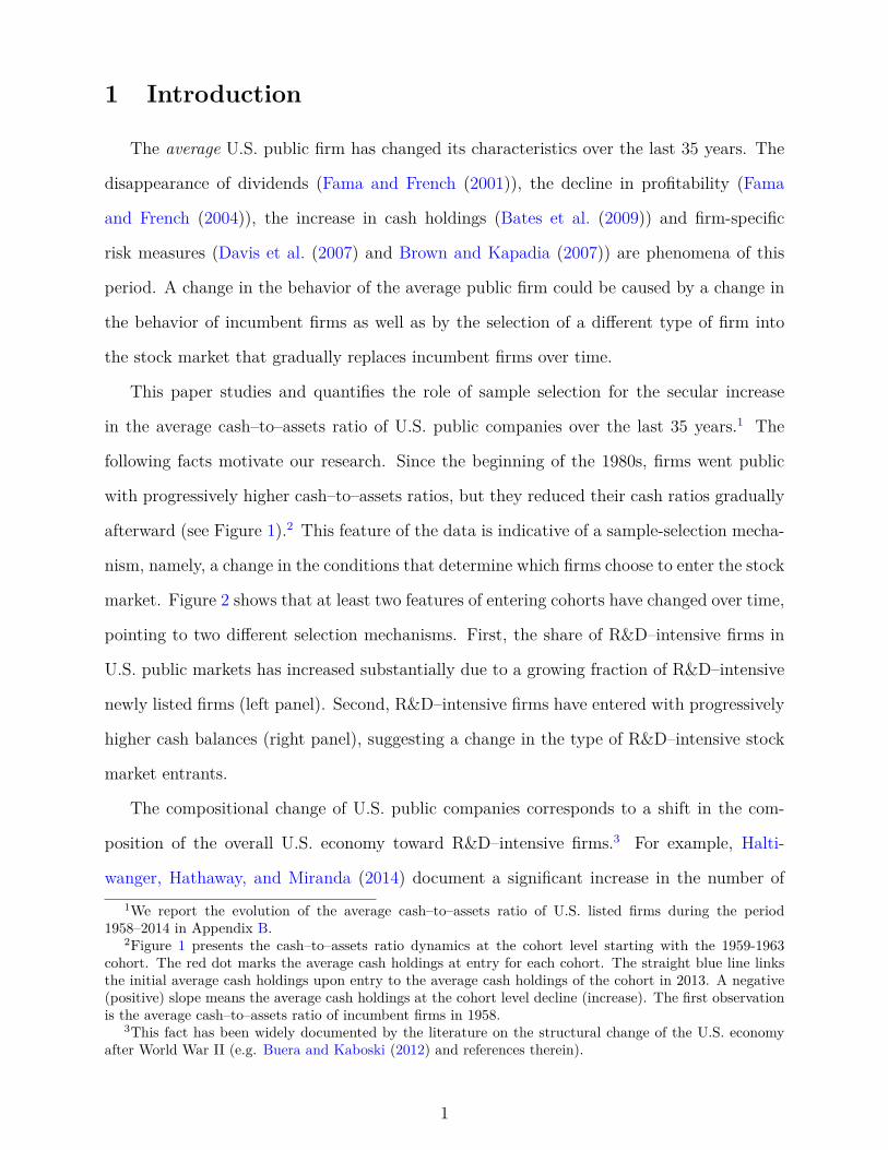
market. Figure 2 shows that at least two features of entering cohorts have changed over time,
pointing to two different selection mechanisms. First, the share of R&D–intensive firms in
U.S. public markets has increased substantially due to a growing fraction of R&D–intensive
newly listed firms (left panel). Second, R&D–intensive firms have entered with progressively
higher cash balances (right panel), suggesting a change in the type of R&D–intensive stock
market entrants.
The compositional change of U.S. public companies corresponds to a shift in the com-
position of the overall U.S. economy toward R&D–intensive firms.3 For example, Halti-
wanger, Hathaway, and Miranda (2014) document a significant increase in the number of1We report the evolution of the average cash–to–assets ratio of U.S. listed firms during the period
1958–2014 in Appendix B.2Figure 1 presents the cash–to–assets ratio dynamics at the cohort level starting with the 1959-1963
cohort. The red dot marks the average cash holdings at entry for each cohort. The straight blue line linksthe initial average cash holdings upon entry to the average cash holdings of the cohort in 2013. A negative(positive) slope means the average cash holdings at the cohort level decline (increase). The first observationis the average cash–to–assets ratio of incumbent firms in 1958.
3This fact has been widely documented by the literature on the structural change of the U.S. economyafter World War II (e.g. Buera and Kaboski (2012) and references therein).
1
Figure 1: Average Cash Holdings at Entry (1959-2013)
1958
59-6
364
-68
69-7
374
-78
79-8
384
-88
89-9
394
-98
99-0
304
-08
09-1
320
130.05
0.1
0.15
0.2
0.25
0.3
0.35
0.4
0.45
0.5
The figure reports the evolution of the cash–to–assets ratio for U.S. public companies for 11 5-year cohortsover the period 1959-2013. The red dot denotes the average cash ratio at entry for each cohort. The firstobservation denotes the average cash holdings of incumbent firms in 1958. The straight line connects theinitial average cash holdings to the average holding in 2013 for each cohort.
Figure 2: Industry Composition of U.S. Public Firms (1959-2013)
59-6
364
-6869
-7374
-7879
-8384
-8889
-9394
-9899
-0304
-0809
-13
0.25
0.3
0.35
0.4
0.45
0.5
0.55
0.6
0.65
0.7
0.75Fraction of R&D-Intensive Firms
All R&D-Intensive FirmsR&D-Intensive Entrants
59-6
364
-6869
-7374
-7879
-8384
-8889
-9394
-9899
-0304
-0809
-13
0
0.1
0.2
0.3
0.4
0.5
0.6Cash Holdings at Entry
R&D Non-R&D
The left panel of this figure presents the share of R&D–intensive firms in Compustat (in darker color with adashed line) and the share of R&D–intensive entrants (in red with a solid line). The right panel shows theaverage cash–to–assets ratio at entry of R&D–intensive and non–R&D–intensive firms. A R&D–intensivefirm belongs to an industry (three-level digit SIC code) whose average R&D investment amounts to at least2% of assets over the sample period. We group firms into cohorts of five years starting from 1959. We defineas entrant a firms that reports a fiscal year-end value of the stock price for the first time (item PRCC F ).
2
high-tech startups during the period 1982–2007 relative to other startups. A larger ratio of
R&D–intensive to non R&D–intensive firms in the economy increases the likelihood of an
IPO by R&D–intensive firms, all else being equal.
The increase in cash holdings of newly listed R&D–intensive firms suggests each new
cohort to the stock market has different characteristics. Indeed, over time newly listed firms
are smaller, less profitable, and appear to exhibit higher cash-flow volatility compared to
previous cohorts. In the spirit of Fama and French (2004), the selection of a different type
of firm could be driven by more favorable IPO conditions that have allowed weaker firms to
go public (i.e., “a downward shift in the supply curve for new list equity funding” Fama and
French (2004, page 233)). Such a change could have been instigated by the relaxation of
the Employment Retirement Income Security Act’s (ERISA) “Prudent Man” Rule passed by
Congress in 1979 that induced pension funds to invest in riskier (i.e., smaller, less profitable,
and higher growth option) ventures.4 The ensuing improvement in IPO conditions for risky
firms might have particularly benefited R&D–intensive firms, as indicated by Figure 2.
In the first part of this paper, we build a stylized firm industry model with endogenous
entry to gain insights into how these two selection mechanisms can shape the secular increase
in cash holdings. The benefit of a model is that we can isolate confounding effects and develop
testable predictions. In the second part of the paper, we test whether the data corroborate
the model’s predictions.
Our firm industry model assumes firms belong to two sectors that share the same pro-
duction technology and financing opportunities. We interpret old-economy firms as non-
R&D–intensive and new-economy firms as R&D–intensive. Guided by the evidence in Fig-
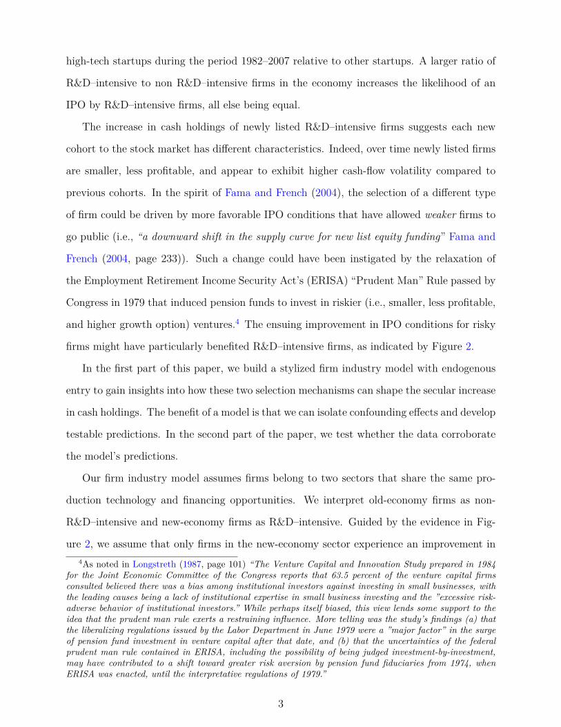
ure 2, we assume that only firms in the new-economy sector experience an improvement in4As noted in Longstreth (1987, page 101) “The Venture Capital and Innovation Study prepared in 1984
for the Joint Economic Committee of the Congress reports that 63.5 percent of the venture capital firmsconsulted believed there was a bias among institutional investors against investing in small businesses, withthe leading causes being a lack of institutional expertise in small business investing and the ”excessive risk-adverse behavior of institutional investors.” While perhaps itself biased, this view lends some support to theidea that the prudent man rule exerts a restraining influence. More telling was the study’s findings (a) thatthe liberalizing regulations issued by the Labor Department in June 1979 were a ”major factor” in the surgeof pension fund investment in venture capital after that date, and (b) that the uncertainties of the federalprudent man rule contained in ERISA, including the possibility of being judged investment-by-investment,may have contributed to a shift toward greater risk aversion by pension fund fiduciaries from 1974, whenERISA was enacted, until the interpretative regulations of 1979.”
3

the conditions that influence their entry decisions. A reduction in entry costs causes firms
with lower idiosyncratic productivity (i.e., less profitable firms with high growth potential)
to go public. The assumed mean reversion in the productivity process implies these firms
have higher funding needs and choose higher cash balances at entry to save up for future
investment opportunities in order to avoid equity issuance costs. As these firms grow, they
reduce their cash holdings given that they can rely more on internal funds, thus making the
model consistent with the evidence in Figure 1.
The model predicts that the first selection mechanism, a change in the industry compo-
sition at entry (across-industry selection), plays no role in shaping the secular increase in
cash. However, it provides an important amplification mechanism when coupled with the
entry of less-profitable, high-growth-potential new-economy firms (intra-industry selection).
This second selection effect is necessary to generate increasing cash holdings at entry over
time that, in turn, lead to a steady increase in the average cash–to–assets ratio in the cross
section. In addition, the model suggests the turnover ratio plays a major role in determining
the cash holdings of entering firms given its tight connection with firm-level profitability
since the ratio of sales over total assets is proportional to profitability in the model.
In the second part of the paper, we measure the importance of sample selection in de-
termining the secular increase in cash, and test the model’s predictions in the data. We
first show that sample selection is a major cause for the secular increase in cash holdings.
Our evidence is straightforward. On average, firms deplete their cash holdings over time,
as measured by a negative time trend within firms. Yet, on average, firms’ cash holdings
have increased. Thus, the increase in cash holdings is a consequence of newly listed firms
increasing their cash holdings at entry faster than the rate at which incumbents deplete
theirs. Using a simple accounting identity, we decompose the change in the average cash-to-
assets ratio over the period 1979–2013 (0.151) in the contribution due to the entry margin
(sample-selection effect) and the contribution due to incumbent firms (within effect). We
show that sample selection accounts for more than 200% of the secular increase in cash
holdings (0.329), whereas the contribution of the within change is actually -117% (-0.178).
Next, we present evidence for the two selection mechanisms our model highlights. To this
4
end, we construct random subsamples from the data that control for both selection effects
so that (1) R&D–intensive entrants in the stock market have an average cash–to–assets ratio
as in 1974-1978 (pre-secular increase), and (2) the proportion of R&D–intensive entrants
is the same as in 1974-1978. When both restrictions are imposed, we can hardly generate
a positive trend in average cash holdings. At the same time, R&D–intensive entrants are
relatively larger and more efficient (i.e., higher turnover ratio) compared to the data, as
predicted by the model. Allowing for an across-industry selection mechanism by lifting
restriction (2) results in a small increase in average cash holdings that is not large enough
to fit the data. Moreover, R&D–intensive entrants are larger and exhibit higher turnover
ratios compared to the actual sample. Lifting only restriction (1), that is, allowing for an
intra-industry selection, results in R&D–intensive entrants whose evolution of characteristics
in terms of size and turnover ratios are in line with the data. As predicted by the model,
average cash holdings increase, but not by as much as to match the data. For this to happen,
we need to lift both restrictions so that the across-industry selection mechanism amplifies
the effects of the intra-industry selection mechanism.
In our model, the turnover ratio is proportional to firm-level productivity and, as such, is
an important determinant for cash holdings at entry. We conclude the empirical analysis by
assessing the explanatory power of the latter variable. We find the turnover ratio is indeed
an important predictor of cash holdings at entry, and its dominant explanatory power is not
subdued when we include a set of important determinants of corporate cash holdings that
have been discussed in the literature.
Our paper contributes to the debate on the causes of the increase in cash holdings
among U.S. publicly listed firms.5 A rich literature uses heterogeneous dynamic corpo-5The literature on the determinants of cash holdings is extensive and ranges over many decades. A classic
motive for holding cash is transaction costs (e.g., Baumol (1952), Tobin (1956), Miller and Orr (1966), andVogel and Maddala (1967)). Other motives include taxes (e.g., Foley, Hartzell, Titman, and Twite (2007)),precautionary savings (e.g., Froot, Scharfstein, and Stein (1993), Kim et al. (1998)), and agency costs (e.g.,Jensen (1986), Dittmar and Mahrt-Smith (2007) and Nikolov and Whited (2014)). Opler et al. (1999) providean extensive test of these different motives. In the last decade, the secular increase in cash holdings hasreceived much attention and spurred many explanations that are not based on sample selection, for example,a tax-based explanation by Foley, Hartzell, Titman, and Twite (2007) and Faulkender and Petersen (2012), aprecautionary savings motive by Bates, Kahle, and Stulz (2009), McLean (2011), and Zhao (2015), operativechanges by Falato, Kadyrzhanova, and Sim (2013) and Gao (2015), as well as the cost of carrying cash (e.g.Azar, Kagy, and Schmalz (2016) and Curtis, Garin, and Mehkari (2015)).
5
rate finance models to understand and quantify corporate cash policies (e.g., Gamba and
Triantis (2008), Riddick and Whited (2009), Anderson and Carverhill (2012), and Nikolov
and Whited (2014)) as well as the secular increase in cash holdings (e.g., Falato et al. (2013),
Gao (2015), Zhao (2015), Armenter and Hnatkovska (2016), Chen et al. (2017)). The firm’s
optimization problem in our model is based on Riddick and Whited (2009). To the best of
our knowledge, our stylized model provides one of the first dynamic corporate finance models
that explicitly allows for the presence of various selection mechanisms and is qualitatively
consistent with the stylized facts we document in Figures 1 and 2.
Heckman (1979) highlighted how ignoring sample selection can lead to biased estimates.
In our model, the standard decreasing returns-to-scale assumption in combination with the
entry of less profitable firms over time is sufficient to generate higher cash–to–assets ratios and
higher sales-growth volatility. Empirical estimates that do not control for sample selection
may incorrectly infer that the underlying cash–flow process has become more volatile. Put
differently, those estimates could assign too much importance to increased uncertainty when
in fact selection contributed to the rise in measured cash-flow volatility and cash holdings.6
In this paper, we argue that selection is a key driver for the secular increase in the cash-
to-assets ratio. We are not the first to point out that newly listed firms in R&D–intensive
industries appear to play a role.7 Bates, Kahle, and Stulz (2009) find that high–tech, non-
dividend payers and recently listed firms have successively higher cash ratios, but they also
find an increase in the non-high–tech sectors.8 Booth and Zhou (2013) present evidence that
the increase in the average cash–to–assets ratio is due to changing firm characteristics of
high-tech firms that went public after 1980. In concurrent work, Graham and Leary (2016)
study the determinants of cash policies using data from the 1920s onward to investigate
what factors were most important for cash holdings over different periods. Related to the
period we study, they also find that average cash holdings began to rise in about 1980 even6Roberts and Whited (2013) provide a survey of potential endogeneity issues in empirical corporate
finance.7Several papers find a positive relationship between cash and R&D expenditures (e.g., Opler and Titman
(1994), Opler, Pinkowitz, Stulz, and Williamson (1999), Brown and Petersen (2011), Falato and Sim (2014),He and Wintoki (2014), Lyandres and Palazzo (2015), and Malamud and Zucchi (2016) among many others).
8We discuss this difference in section 3.2 and 3.3.
6

though within-firm cash balances declined over this period. They also attribute the post-
1980 rise in average cash balances to changes in sample composition due to new health and
tech NASDAQ firms going public with large cash balances.9
We expand on these insights by (1) proposing an empirical measure of the selection effect,
(2) providing evidence for the two sample-selection mechanisms advanced by the model, and
(3) highlighting the importance of the turnover ratio (sales over assets) as an important
determinant of cash holdings at entry and therefore the secular increase in cash holdings.
The paper is organized as follows. We present the model in Section 2. The results of the
empirical analysis are in Section 3. We first empirically assess the contribution of sample
selection to the secular increase in cash holdings. Then, in Section 3.4, we explicitly study
the impact of different selection mechanisms. We conclude in Section 3.5 by comparing the
explanatory power of the turnover ratio with other important determinants of corporate cash
holdings.
2 Selection and average cash holdings: insights from a
firm industry model
In this section, we develop a stylized heterogeneous firm industry model to illustrate how
changes in the selection process can be a major driver of the average cash-to-assets ratio over
time. We assume firms belong to one of two sectors labeled as the new-economy sector and
old-economy sector. We set up the firm problem similarly to Riddick and Whited (2009).
That is, firms use a decreasing returns-to-scale technology with capital as the only input.
Firms can finance themselves with equity or with internal funds. We assume a time-invariant
mass of potential firms exists that endogenously decides to become public (i.e., entry in the
stock market). These potential entrants are either new-economy or old-economy firms.
To highlight the effect of the entry margin, both firm types are modeled identically. That
is, we assume firms in both sectors share the same production technology and have the same9Seventy percent of the R&D–intensive entrants in our sample are listed on NASDAQ, while 20% are
listed on the NYSE, and the remainder on AMEX.
7
financing opportunities. The only difference between these sectors is that, contrary to old-
economy firms, new-economy firms experience a change in the conditions that influence their
entry decision.
2.1 Incumbent problem
This section presents the incumbent problem that is identical across both sectors.
Technology Firms produce using the decreasing returns-to-scale production function
yt = ezt+1kαt , where zt+1 is an idiosyncratic productivity shock that evolves according to
zt+1 = ρzt + σεt+1, εt+1i.i.d.∼ N(0, 1).
The law of motion for the capital stock is kt+1 = (1− δ)kt + xt, where δ is the depreciation
rate and xt is the capital investment at time t that entails an adjustment cost equal to
φ(kt+1, kt) = η
(kt+1 − (1− δ)kt
kt
)2
kt.
Financing Firms can finance their operations internally by transferring cash from one
period to the next at an accumulation rate R lower than the (gross) risk-free rate R. In
particular, we assume R = νR, where ν ∈ (0, 1). Firms can also raise external resources
by issuing equity. Equity financing is costly: raising equity (i.e., having a negative dividend
dt < 0) requires the payment of H(dt), where H(dt) = −κ|dt|.
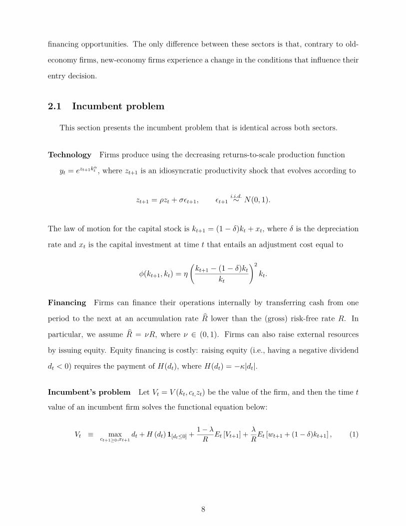
Incumbent’s problem Let Vt = V (kt, ct,zt) be the value of the firm, and then the time t
value of an incumbent firm solves the functional equation below:
Vt ≡ maxct+1≥0,xt+1
dt +H (dt) 1[dt≤0] + 1− λR
Et [Vt+1] + λ
REt [wt+1 + (1− δ)kt+1] , (1)
8
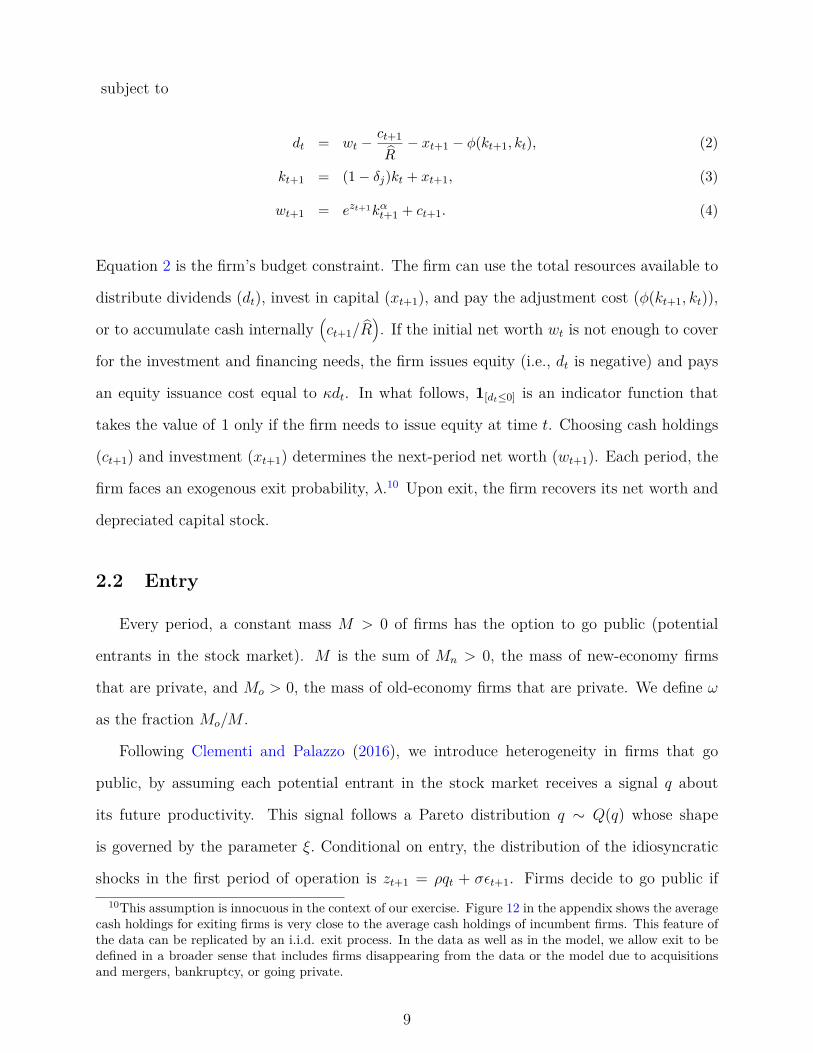
subject to
dt = wt −ct+1
R− xt+1 − φ(kt+1, kt), (2)
kt+1 = (1− δj)kt + xt+1, (3)
wt+1 = ezt+1kαt+1 + ct+1. (4)
Equation 2 is the firm’s budget constraint. The firm can use the total resources available to
distribute dividends (dt), invest in capital (xt+1), and pay the adjustment cost (φ(kt+1, kt)),
or to accumulate cash internally(ct+1/R
). If the initial net worth wt is not enough to cover
for the investment and financing needs, the firm issues equity (i.e., dt is negative) and pays
an equity issuance cost equal to κdt. In what follows, 1[dt≤0] is an indicator function that
takes the value of 1 only if the firm needs to issue equity at time t. Choosing cash holdings
(ct+1) and investment (xt+1) determines the next-period net worth (wt+1). Each period, the
firm faces an exogenous exit probability, λ.10 Upon exit, the firm recovers its net worth and
depreciated capital stock.
2.2 Entry
Every period, a constant mass M > 0 of firms has the option to go public (potential
entrants in the stock market). M is the sum of Mn > 0, the mass of new-economy firms
that are private, and Mo > 0, the mass of old-economy firms that are private. We define ω
as the fraction Mo/M .
Following Clementi and Palazzo (2016), we introduce heterogeneity in firms that go
public, by assuming each potential entrant in the stock market receives a signal q about
its future productivity. This signal follows a Pareto distribution q ∼ Q(q) whose shape
is governed by the parameter ξ. Conditional on entry, the distribution of the idiosyncratic
shocks in the first period of operation is zt+1 = ρqt + σεt+1. Firms decide to go public if10This assumption is innocuous in the context of our exercise. Figure 12 in the appendix shows the average
cash holdings for exiting firms is very close to the average cash holdings of incumbent firms. This feature ofthe data can be replicated by an i.i.d. exit process. In the data as well as in the model, we allow exit to bedefined in a broader sense that includes firms disappearing from the data or the model due to acquisitionsand mergers, bankruptcy, or going private.
9

the value of being a publicly traded firm exceeds the value of staying private Vp. The value
function for a potential entrant is
V E(qt) = maxct+1,xt+1
{−xt+1 −
ct+1
R+ 1RE[V (kt+1, ct+1, zt+1)|qt]
}. (5)
A firm goes public if and only if V E ≥ Vp.11
2.3 The underlying mechanism: mean reversion in productivity
This section describes the tight link between the cash–to–assets ratio of entrants and
their productivity state. Before we go into more detail on this link, we first briefly sketch
out the model parametrization. The firm industry equilibrium and the solution method are
described in the appendix (Section A.1). We parametrize the model at an annual frequency
using calibrated values that match key features of U.S. public firms. The calibration strategy
is laid out in detail in Section A.2. To highlight the role of selection, we calibrate the
parameters listed in Table 1 using the period 1959-1979, that is, before a marked increase
in the cash–to-assets ratio. Panel A lists standard parameters that we borrowed from the
literature. Panel B reports the calibrated parameters, their value, the targeted data moment,
and the equivalent model moments. Finally, Panel C reports the calibration target for the
exit-rate parameter λ that has been chosen to map the age distribution in the model as close
as possible to the age distribution in the data.
The policy functions (Section A.3) are fairly standard. The key insights from those
policy functions is the importance of precautionary financing for small firms. Large firms
have a smaller precautionary savings motive because they rely on larger expected cash flows,
and for this reason, they need to retain less cash when financing constraints are binding.
Conversely, small firms engage in larger precautionary savings, and in doing, so they deliver
a larger cash-to-assets ratio.
This paper stresses the importance of the entry margin, i.e. the selection process. The11We follow a reduced-form approach to model the going-public decision and choose not to model the
problem of the private firm. The selection mechanisms that drive our results will also operate in a morerealistic setup along the lines of Clementi (2002).
10
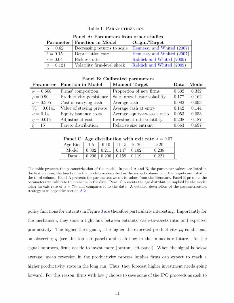
Table 1: Parametrization
Panel A: Parameters from other studiesParameter Function in Model Origin/Targetα = 0.62 Decreasing returns to scale Hennessy and Whited (2007)δ = 0.15 Depreciation rate Hennessy and Whited (2007)r = 0.04 Riskless rate Riddick and Whited (2009)σ = 0.121 Volatility firm-level shock Riddick and Whited (2009)
Panel B: Calibrated parametersParameter Function in Model Moment Target Data Modelω = 0.668 Firms’ composition Proportion of new firms 0.332 0.332ρ = 0.90 Productivity persistence Sales growth rate volatility 0.177 0.162ν = 0.995 Cost of carrying cash Average cash 0.082 0.093Vp = 0.0141 Value of staying private Average cash at entry 0.142 0.144κ = 0.14 Equity issuance costs Average equity-to-asset ratio 0.053 0.053η = 0.015 Adjustment cost Investment rate volatility 0.208 0.187ξ = 15 Pareto distribution Relative size entrant 0.663 0.697
Panel C: Age distribution with exit rate λ = 0.07Age Bins 1-5 6-10 11-15 16-20 >20
Model 0.302 0.211 0.147 0.102 0.238Data 0.296 0.206 0.159 0.119 0.221
The table presents the parametrization of the model. In panel A and B, the parameter values are listed inthe first column, the function in the model are described in the second column, and the targets are listed inthe third column. Panel A presents the parameters we set to values from the literature. Panel B presents theparameters we calibrate to moments in the data. Panel C presents the age distribution implied by the modelusing an exit rate of λ = 7% and compares it to the data. A detailed description of the parametrizationstrategy is in appendix section A.2.
policy functions for entrants in Figure 3 are therefore particularly interesting. Importantly for
the mechanism, they show a tight link between entrants’ cash–to–assets ratio and expected
productivity. The higher the signal q, the higher the expected productivity ρq conditional
on observing q (see the top left panel) and cash flow in the immediate future. As the
signal improves, firms decide to invest more (bottom left panel). When the signal is below
average, mean reversion in the productivity process implies firms can expect to reach a
higher productivity state in the long run. Thus, they forecast higher investment needs going
forward. For this reason, firms with low q choose to save some of the IPO proceeds as cash to
11
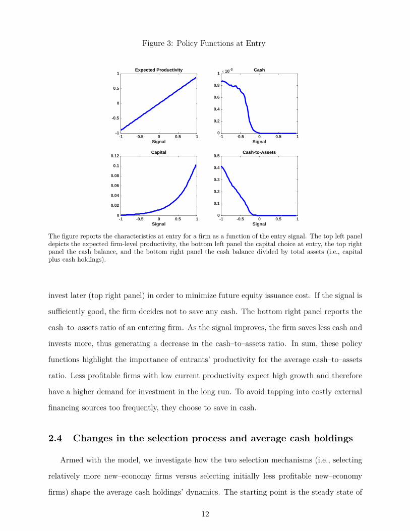
Figure 3: Policy Functions at Entry
Signal-1 -0.5 0 0.5 1
-1
-0.5
0
0.5
1Expected Productivity
Signal-1 -0.5 0 0.5 1
#10-3
0
0.2
0.4
0.6
0.8
1Cash
Signal-1 -0.5 0 0.5 1
0
0.02
0.04
0.06
0.08
0.1
0.12Capital
Signal-1 -0.5 0 0.5 1
0
0.1
0.2
0.3
0.4
0.5Cash-to-Assets
The figure reports the characteristics at entry for a firm as a function of the entry signal. The top left paneldepicts the expected firm-level productivity, the bottom left panel the capital choice at entry, the top rightpanel the cash balance, and the bottom right panel the cash balance divided by total assets (i.e., capitalplus cash holdings).
invest later (top right panel) in order to minimize future equity issuance cost. If the signal is
sufficiently good, the firm decides not to save any cash. The bottom right panel reports the
cash–to–assets ratio of an entering firm. As the signal improves, the firm saves less cash and
invests more, thus generating a decrease in the cash–to–assets ratio. In sum, these policy
functions highlight the importance of entrants’ productivity for the average cash–to–assets
ratio. Less profitable firms with low current productivity expect high growth and therefore
have a higher demand for investment in the long run. To avoid tapping into costly external
financing sources too frequently, they choose to save in cash.
2.4 Changes in the selection process and average cash holdings
Armed with the model, we investigate how the two selection mechanisms (i.e., selecting
relatively more new–economy firms versus selecting initially less profitable new–economy
firms) shape the average cash holdings’ dynamics. The starting point is the steady state of
12

the benchmark model calibrated to data from the 1959-1979 period, where the economy is
populated by identical firms.
The first experiment is designed to explore the effect of a structural change in the com-
position of firms (across-industry selection mechanism) on the average cash-to-assets ratio
(top left panel of Figure 4). To this end, we assume the fraction of potential entrants of type
old ω changes over a time span of 35 years so that the model replicates the compositional
change for publicly traded firms in the data (top right panel of Figure 4).12
A structural change in the composition of entrants is unable to generate a secular increase
in the average cash holdings of publicly traded firms. The solid blue lines in the bottom
panels of Figure 4 show the increase in average cash holdings for new-economy firms (bottom
left panel) is due to the increase in the proportion of young firms (bottom right panel). Given
that exit is i.i.d., a progressively larger fraction of new-economy entrants leads to an increase
in the proportion of young new-economy firms. These firms are smaller and have, on average,
larger cash-to-assets ratios relative to their more mature counterparts.
This positive effect on average cash holdings is counterbalanced by the dynamics of
cash holdings for old-economy firms, as illustrated by the dashed red lines in the bottom
panels of Figure 4. Because old economy firms enter in a smaller number, their composition
shifts toward more mature firms that have, on average, lower cash-to-assets ratios. This
effects leads to an initial decrease of average cash holdings. It follows that the cash-holdings
dynamics in the two sectors offset each other, thus leaving the overall cash-to-assets ratio
unchanged over time, as described by the top left panel of Figure 4. Without a change in
the characteristics at entry of new-economy firms, the model cannot generate an increase in
average cash holdings.
Our second experiment investigates how a change in the characteristics of new-economy
entrants (intra-industry selection) affects the cash–to–assets ratio. Motivated by the changes
to institutional investors’ investment opportunities at the end of the 1970s discussed in the12To be precise, we assume the fraction of potential entrants of type old evolves over time according to
ωt = (ω − a1) + a1t−a2 , where t = 1, ..., 35. We pick a1 and a2 to minimize the distance between the
compositional change generated by the model and the one observed in the data. The calibrated values of a1and a2 deliver a fraction of potential entrants of type old equal to 40% after 35 years.
13
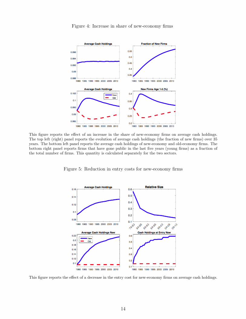
Figure 4: Increase in share of new-economy firms
This figure reports the effect of an increase in the share of new-economy firms on average cash holdings.The top left (right) panel reports the evolution of average cash holdings (the fraction of new firms) over 35years. The bottom left panel reports the average cash holdings of new-economy and old-economy firms. Thebottom right panel reports firms that have gone public in the last five years (young firms) as a fraction ofthe total number of firms. This quantity is calculated separately for the two sectors.
Figure 5: Reduction in entry costs for new-economy firms
This figure reports the effect of a decrease in the entry cost for new-economy firms on average cash holdings.
14
introduction, we study the response of the model to a reduction in the value of staying private
for new-economy firms. We assume a reduction in Vp over 35 years to mimic the dynamics
of the relative size of entering firms.13 Figure 5 shows this change reduces the threshold
productivity level for entry. That is, even small (top right panel) and less productive firms
(i.e., low-profitability firms with higher growth potential) choose to go public. Because
the shocks are mean reverting, lower-productivity firms anticipate higher productivity in the
future and raise more cash relative to their assets at the IPO stage (bottom right panel). This
behavior is a natural consequence of the entrants’ policy function discussed in section 2.3.
This selection mechanism only affects the average cash-to-assets ratio of new-economy firms
(bottom left panel), thus replicating the empirical evidence in Figure 2 of R&D–intensive
firms entering with progressively higher cash balances. The model can explain around 26%
of the total change in cash holdings.14
On its own, neither selection mechanism is quantitatively strong enough to explain the
secular trend in cash holdings. However, the combination of the intra-industry selection effect
with the across-industry selection effect - a purely selection-based mechanism - explains 46%
of the trend.
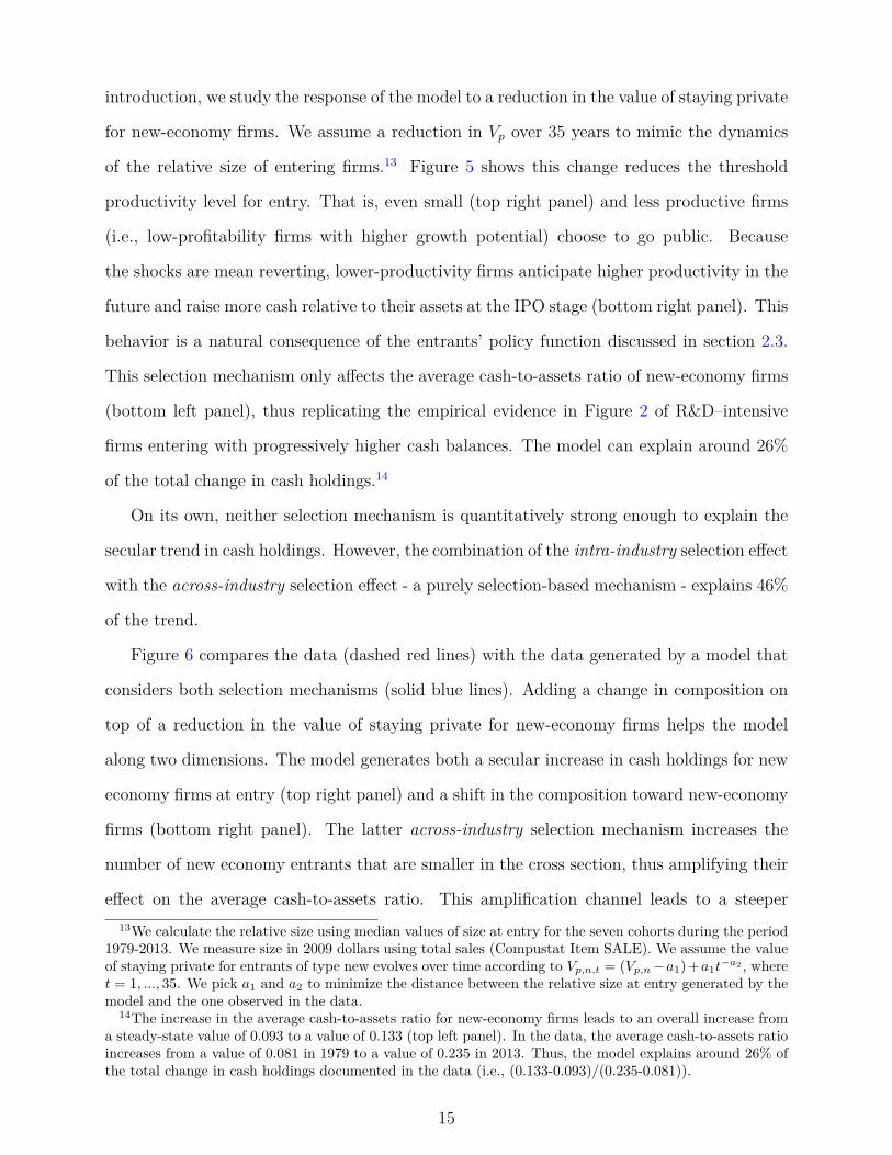
Figure 6 compares the data (dashed red lines) with the data generated by a model that
considers both selection mechanisms (solid blue lines). Adding a change in composition on
top of a reduction in the value of staying private for new-economy firms helps the model
along two dimensions. The model generates both a secular increase in cash holdings for new
economy firms at entry (top right panel) and a shift in the composition toward new-economy
firms (bottom right panel). The latter across-industry selection mechanism increases the
number of new economy entrants that are smaller in the cross section, thus amplifying their
effect on the average cash-to-assets ratio. This amplification channel leads to a steeper13We calculate the relative size using median values of size at entry for the seven cohorts during the period
1979-2013. We measure size in 2009 dollars using total sales (Compustat Item SALE). We assume the valueof staying private for entrants of type new evolves over time according to Vp,n,t = (Vp,n−a1)+a1t
−a2 , wheret = 1, ..., 35. We pick a1 and a2 to minimize the distance between the relative size at entry generated by themodel and the one observed in the data.
14The increase in the average cash-to-assets ratio for new-economy firms leads to an overall increase froma steady-state value of 0.093 to a value of 0.133 (top left panel). In the data, the average cash-to-assets ratioincreases from a value of 0.081 in 1979 to a value of 0.235 in 2013. Thus, the model explains around 26% ofthe total change in cash holdings documented in the data (i.e., (0.133-0.093)/(0.235-0.081)).
15
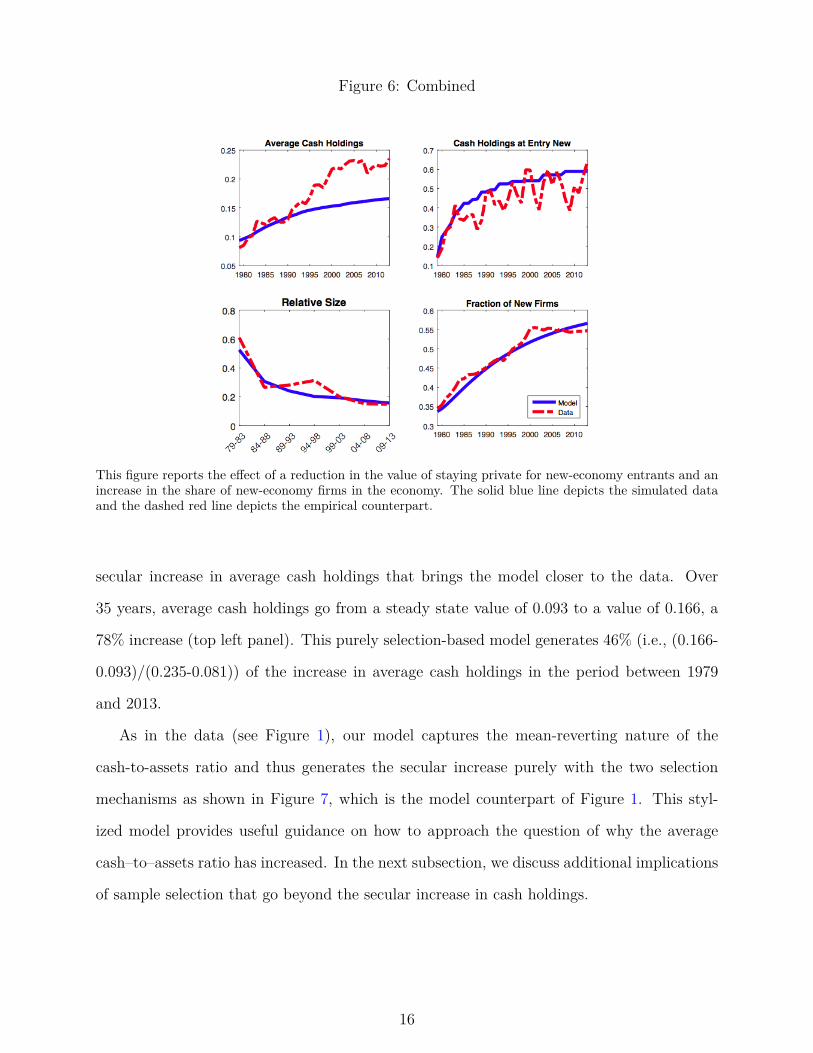
Figure 6: Combined
This figure reports the effect of a reduction in the value of staying private for new-economy entrants and anincrease in the share of new-economy firms in the economy. The solid blue line depicts the simulated dataand the dashed red line depicts the empirical counterpart.
secular increase in average cash holdings that brings the model closer to the data. Over
35 years, average cash holdings go from a steady state value of 0.093 to a value of 0.166, a
78% increase (top left panel). This purely selection-based model generates 46% (i.e., (0.166-
0.093)/(0.235-0.081)) of the increase in average cash holdings in the period between 1979
and 2013.
As in the data (see Figure 1), our model captures the mean-reverting nature of the
cash-to-assets ratio and thus generates the secular increase purely with the two selection
mechanisms as shown in Figure 7, which is the model counterpart of Figure 1. This styl-
ized model provides useful guidance on how to approach the question of why the average
cash–to–assets ratio has increased. In the next subsection, we discuss additional implications
of sample selection that go beyond the secular increase in cash holdings.
16
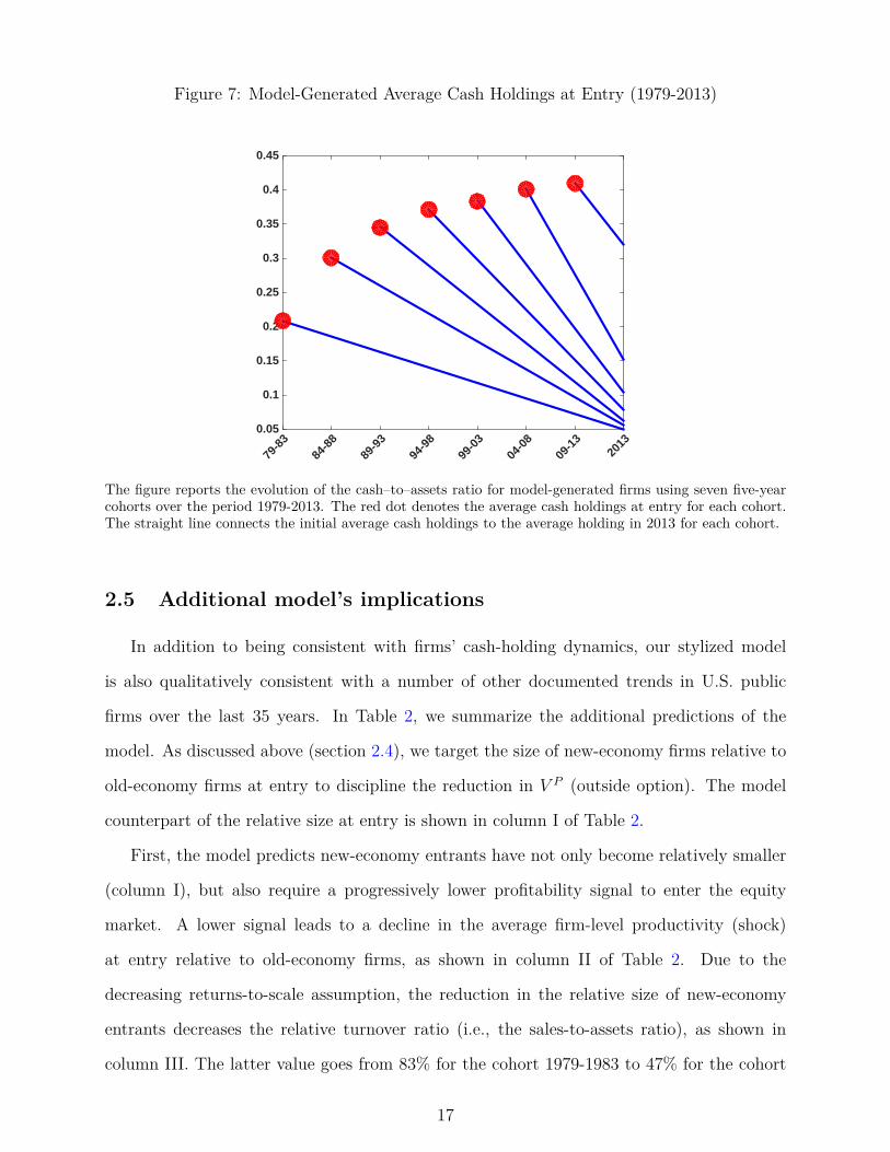
Figure 7: Model-Generated Average Cash Holdings at Entry (1979-2013)
79-8
384
-88
89-9
394
-98
99-0
304
-08
09-1
320
130.05
0.1
0.15
0.2
0.25
0.3
0.35
0.4
0.45
The figure reports the evolution of the cash–to–assets ratio for model-generated firms using seven five-yearcohorts over the period 1979-2013. The red dot denotes the average cash holdings at entry for each cohort.The straight line connects the initial average cash holdings to the average holding in 2013 for each cohort.
2.5 Additional model’s implications
In addition to being consistent with firms’ cash-holding dynamics, our stylized model
is also qualitatively consistent with a number of other documented trends in U.S. public
firms over the last 35 years. In Table 2, we summarize the additional predictions of the
model. As discussed above (section 2.4), we target the size of new-economy firms relative to
old-economy firms at entry to discipline the reduction in V P (outside option). The model
counterpart of the relative size at entry is shown in column I of Table 2.
First, the model predicts new-economy entrants have not only become relatively smaller
(column I), but also require a progressively lower profitability signal to enter the equity
market. A lower signal leads to a decline in the average firm-level productivity (shock)
at entry relative to old-economy firms, as shown in column II of Table 2. Due to the
decreasing returns-to-scale assumption, the reduction in the relative size of new-economy
entrants decreases the relative turnover ratio (i.e., the sales-to-assets ratio), as shown in
column III. The latter value goes from 83% for the cohort 1979-1983 to 47% for the cohort
17
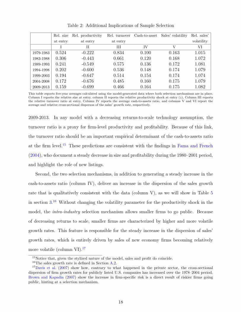
Table 2: Additional Implications of Sample Selection
Rel. size Rel. productivity Rel. turnover Cash-to-asset Sales’ volatility Rel. sales’at entry at entry at entry volatility
I II III IV V VI1979-1983 0.524 -0.222 0.834 0.100 0.163 1.0151983-1988 0.306 -0.443 0.661 0.120 0.168 1.0721989-1993 0.241 -0.549 0.575 0.136 0.172 1.0811994-1998 0.202 -0.600 0.536 0.148 0.174 1.0791999-2003 0.194 -0.647 0.514 0.154 0.174 1.0742004-2008 0.172 -0.676 0.485 0.160 0.175 1.0792009-2013 0.159 -0.699 0.466 0.164 0.175 1.082
This table reports five-year averages calculated using the model-generated data where both selection mechanisms are in place.Column I reports the relative size at entry, column II reports the relative productivity shock at entry (z), Column III reportsthe relative turnover ratio at entry, Column IV reports the average cash-to-assets ratio, and columns V and VI report theaverage and relative cross-sectional disperson of the sales’ growth rate, respectively.
2009-2013. In any model with a decreasing returns-to-scale technology assumption, the
turnover ratio is a proxy for firm-level productivity and profitability. Because of this link,
the turnover ratio should be an important empirical determinant of the cash-to-assets ratio
at the firm level.15 These predictions are consistent with the findings in Fama and French
(2004), who document a steady decrease in size and profitability during the 1980–2001 period,
and highlight the role of new listings.
Second, the two selection mechanisms, in addition to generating a steady increase in the
cash-to-assets ratio (column IV), deliver an increase in the dispersion of the sales growth
rate that is qualitatively consistent with the data (column V), as we will show in Table 5
in section 3.16 Without changing the volatility parameter for the productivity shock in the
model, the intra-industry selection mechanism allows smaller firms to go public. Because
of decreasing returns to scale, smaller firms are characterized by higher and more volatile
growth rates. This feature is responsible for the steady increase in the dispersion of sales’
growth rates, which is entirely driven by sales of new economy firms becoming relatively
more volatile (column VI).17
15Notice that, given the stylized nature of the model, sales and profit do coincide.16The sales growth rate is defined in Section A.2.17Davis et al. (2007) show how, contrary to what happened in the private sector, the cross-sectional
dispersion of firm growth rates for publicly listed U.S. companies has increased over the 1978–2004 period.Brown and Kapadia (2007) show the increase in firm-specific risk is a direct result of riskier firms goingpublic, hinting at a selection mechanism.
18
To sum up, our model suggests that any data analysis should pay attention to entry de-
cisions of firms, particularly when a specific firm type (here R&D–intensive firms) becomes
increasingly dominant in the sample. Inference based on exogenous changes in deep param-
eters (e.g., an increase in the cash–flow volatility parameter over time) can be confounded
with factors that are outside the firm’s optimization problem, but are due to changes in the
selection process into the stock market. For example, empirical estimates could assign too
much importance to increased uncertainty when in fact selection contributes to the rise in
cash-flow volatility and cash holdings.
3 The empirical evidence on sample selection effects
In this section, we explore the model’s predictions by studying how sample selection
affects the secular increase in the cash–to–assets ratio. The data corroborate what the
model suggests: most of the action for the change in the cash–to–assets ratio is at the entry
margin and is driven by an increasing share of smaller and less profitable R&D–intensive
firms with higher cash-to-assets ratios that went public during the last 35 years.
We first describe the data set and definitions. Then we show a negative time trend exists
in the cash–to–assets ratio at the firm level, whereas pooled OLS regressions show a positive
time trend. A negative firm-level trend together with a positive trend in the cross-section
suggests the secular increase in cash is mainly a byproduct of sample selection. We isolate the
effect of sample selection on the positive time trend using a simple accounting decomposition
and show that newly listed R&D–intensive firms are responsible for the bulk in the increase
of the average cash-to-assets ratio.18 We conclude our analysis by providing evidence for
the two selection mechanisms discussed in the model and by studying the determinants of
R&D–intensive firms’ cash holdings before they go public.18We rule out firm exit as a driver of the secular increase in the cash–to–assets ratio (see figure 12 in the
appendix). We find the average cash–to–assets ratio at exit is close to the cross-sectional average of thecash–to–assets ratio. This behavior is consistent with exit being i.i.d.
19
3.1 R&D–intensive firms: Data and definitions
We use annual Compustat data for the period 1959-2013, excluding financial firms (SIC
codes 6000 to 6999) and regulated industries (SIC codes 4000 to 4999), non-U.S.-incorporated
firms, and those not traded on the three major exchanges: NYSE, AMEX, and NASDAQ.
R&D–intensive firms are firms that belong to an industry (using the three-level-digit
SIC code) that has an average R&D investment–to–assets ratio of at least 2%. We choose
2% as the cut-off level because it is the minimum R&D–to–asset ratios of the top quintile
industries in terms of R&D to assets.19
Our R&D–based industry classification is consistent with other classifications used in
previous empirical studies. The seven industries that account for the bulk of R&D–intensive
entrants are the same industries Brown et al. (2009) use to identify the high–tech sector.
In addition, our broadly defined R&D–intensive sector contains all the industries classified
as “Internet and Technology Firms” by Loughran and Ritter (2004), with the exception of
Telephone Equipment (SIC 481), which we exclude by construction because it belongs to a
regulated industry.20
We want to follow the dynamics of an entering cohort. To this end, we sort firms into
seven cohorts using non-overlapping periods of five years starting with the window 1979-
1983. A cohort definition based on a five-year window is fairly standard in the firm-dynamics
literature but not essential to our results. We define an entrant as a firm that reports a
fiscal year-end value of the stock price for the first time (item PRCC F ).21
19We obtain very similar results if we narrow our definition down to using the seven specific industriesthat account for the bulk of R&D–intensive entrants: Computer and Data Processing Services (SIC 737,26% of total entrants), Drugs (SIC 283, 15%), Medical Instruments and Supplies (SIC 384, 9%), ElectronicComponents and Accessories (SIC 367, 8%), Computer and Office Equipment (SIC 357, 7%), Measuringand Controlling Devices (SIC 382, 5%), and Communications Equipment (SIC 366, 5%).
20Differently from Bates et al. (2009), we do not to follow the classification in Loughran and Ritter(2004), because it excludes one of the most relevant R&D–intensive industries (Drugs, SIC 283) from theR&D–intensive sector.
21Our results are robust to using value-weighted data (e.g., Table 11 in the Appendix) or defining entrybased on the IPO dates provided by Jay Ritter. http://bear.warrington.ufl.edu/ritter/ipodata.htm.
20
Tabl
e3:
Estim
atin
gth
eT
ime
Tren
d
Pool
edO
LSFi
rm-b
y-Fi
rmA
llA
llA
llA
llYo
ung
Youn
gM
atur
eM
atur
eO
ldO
ldI
IIII
IIV
VV
IV
IIV
III
IXX
Tren
d0.
418*
**0.
055*
**-0
.497
***
-0.2
67**
*-0
.461
***
-0.2
39**
*-0
.226
***
-0.1
15**
*0.
005
0.00
10.
007
0.00
60.
034
0.04
80.
037
0.05
30.
026
0.03
70.
239
0.03
3
Tren
dX
R&
D0.
605*
**-0
.463
***
-0.4
47**
*-0
.224
***
0.00
70.
013
0.06
80.
075
0.05
20.
048
R&
DD
umm
y4.
579*
**20
.711
***
20.7
60**
*0.
180*
**11
.100
***
0.25
30.
587
0.64
20.
000
0.91
0
Con
stan
t10
.661
***
9.37
1***
21.9
20**
*11
.640
***
21.5
81**
*11
.276
***
20.2
34**
*11
.446
***
14.6
48**
*9.
510*
**0.
123
0.12
20.
325
0.41
30.
350
0.45
30.
387
0.50
50.
474
0.61
9
Obs
erva
tions
85,9
4785
,947
(5,4
96;1
6)(5
,496
;5)
(3,6
14;9
)(1
607;
13)
Adj
uste
dR
20.
035
0.18
50.
295
0.41
80.
312
0.29
1W
ees
timat
eth
efo
llow
ing
base
line
linea
req
uatio
n:
CHi,t
=α
+βt
+ε i,t
The
depe
nden
tva
riabl
eis
the
cash
–to–
asse
tsra
tiode
fined
asC
ompu
stat
item
CH
Edi
vide
dby
Com
pust
atite
mAT
and
expr
esse
din
perc
enta
gete
rms.
The
sam
ple
incl
udes
Com
pust
atfir
m-y
ear
obse
rvat
ions
from
1979
-201
3w
ithat
leas
tfiv
eye
ars
ofob
serv
atio
ns,
posit
ive
valu
esfo
ras
sets
and
sale
s,ex
clud
ing
finan
cial
firm
s(S
ICco
des
6000
to69
99)
and
utili
ties
(SIC
code
s40
00to
4999
).W
eal
soso
rtfir
ms
into
R&
D–
vers
usno
n-R
&D
–int
ensiv
e,as
disc
usse
din
sect
ion
3.1.
Inco
lum
nsI
and
II,w
eru
npo
oled
OLS
regr
essio
nsan
dw
eno
rmal
ize
the
year
1979
toze
ro.
Inco
lum
nsII
I-X
,we
run
alin
ear
regr
essio
nfo
rea
chfir
min
our
sam
ple
and
set
the
time
varia
ble
equa
lto
zero
the
first
year
the
firm
appe
ars
inth
esa
mpl
e.Yo
ung
firm
sar
efir
ms
that
have
been
publ
icfo
rat
mos
tfiv
eye
ars,
mat
ure
firm
sar
efir
ms
that
have
been
publ
icfo
rm
ore
than
five
year
sbu
tle
ssth
an16
year
s,an
dol
dfir
ms
are
firm
sth
atha
vebe
enpu
blic
for
atle
ast
16ye
ars.
For
the
firm
-by-
firm
regr
essio
ns,w
ere
port
the
num
ber
ofin
divi
dual
firm
sin
the
sam
ple
toge
ther
with
the
aver
age
num
ber
ofob
serv
atio
nsfo
rea
chfir
m.
The
repo
rted
R2
for
the
firm
-by-
firm
regr
essio
nsis
the
aver
ageR
2ac
ross
allt
here
gres
sions
.W
ere
port
robu
stst
anda
rder
rors
.*
deno
tes
signi
fican
ceat
the
10%
leve
l,**
deno
tes
signi
fican
ceat
the
5%le
vel,
and
***
deno
tes
signi
fican
ceat
the
1%le
vel.
21
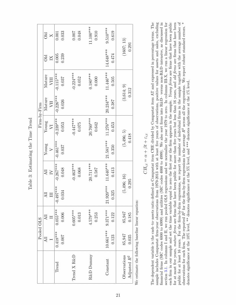
3.2 The time trend in cash holdings
The model presented in Section 2 is able to generate a positive trend in cash holdings
despite the mean-reverting nature of the cash-to-assets ratio at the firm level, which means
that new entrants deplete cash at a lower rate than the rate at which they increase cash at
entry, as illustrated in Figure 7. In this section, we provide evidence for this selection-based
explanation.
We first estimate the time trend in the cash–to–assets ratio using all firms over the period
1979–2013. The resulting trend is positive: cash holdings represented around 11% of total
assets for the typical firm in 1979, and they have increased by 14% over the subsequent
35 years (column I of Table 3). Column II of Table 3 shows the differences in the time
trend across sectors by including a dummy variable that takes a value of zero if a firm is
non-R&D–intensive, and 1 otherwise. The estimated slope for the R&D sector is one order
of magnitude larger than the estimated slope for the non-R&D sector (66 b.p. vs. 5.5 b.p.).
The implied increase in cash holdings for the non–R&D sector over the 35-year period is very
small (around 2%), while cash holdings in the R&D sector surged from an average value of
14% in 1979 to an average value of 35% in 2013. The secular increase in the cash-to-assets
ratio appears to be a phenomenon that pertains almost exclusively to the R&D–intensive
sector.
Pooled OLS regressions allow us to identify R&D–intensive firms as the driver of the sec-
ular increase in cash holdings. However, the cash–to–assets ratio is fairly persistent (see also
Figure 13 and Lemmon et al. (2008)), and pooled OLS regressions are not conclusive with
regard to each firm’s individual cash–to–assets evolution. In fact, incumbent R&D–intensive
firms could have indeed increased their cash–to–assets ratios over time. To address the
persistence issue, we perform firm–by–firm regressions and report average values of the esti-
mated coefficients. We set the time variable equal to zero the first year the firm appears in
the sample. In this way, we control for the cash holdings at entry at the firm level. The re-
sults show a negative change in average cash holdings for incumbents. The estimated yearly
within-firm change in average cash holdings over 35 years is -50 b.p. (column III). Column
22

IV shows that R&D–intensive firms start with much larger cash balances and deplete cash
faster than non-R&D–intensive firms.
The estimates in columns III and IV represent the trend for an average public firm during
the 1979–2013 period. In the remaining columns of Table 3, we estimate the time-trend-
by-age category because firms might not be at their steady-state cash level shortly after the
IPO. In particular, we define young firms as firms that have been public for at most five
years, mature firms as firms that have been public for more than five years but less than 16,
and old firms as firms that have been public for at least 16 years. The results in columns
V-VIII show that (i) both young and mature firms deplete cash after an IPO, (ii) young
firms deplete cash faster than mature firms, and (iii) the estimated slope for R&D–intensive
firms is twice as large as the estimated slope for non–R&D–intensive firms. No significant
time trend in cash holdings exists for old firms (see columns IX and X) regardless of the
sector.
The data show that a positive time trend in average cash holdings exists despite a negative
time trend within firms. As in the model, this feature is a result of newly listed firms
increasing their cash holdings at entry faster than the rate at which incumbents deplete
theirs.22
3.3 Decomposing the change in the average cash ratio
In this section, we directly measure the contribution of sample selection to the secular
increase in average cash holdings. Using a simple accounting decomposition, we find selection
contributes by more than 200%, whereas the within-firm change in cash holdings contributes
a negative 120%.
The accounting decomposition allows us to isolate the part of the change in the average
cash–to–assets ratio coming from changes within incumbent firms from changes due to new
firms (entrants). The change in the average cash–to–assets ratio ∆CHt between time t− 122In the Appendix, we show in Table 9 which entering cohorts have mattered for the secular trend.
23
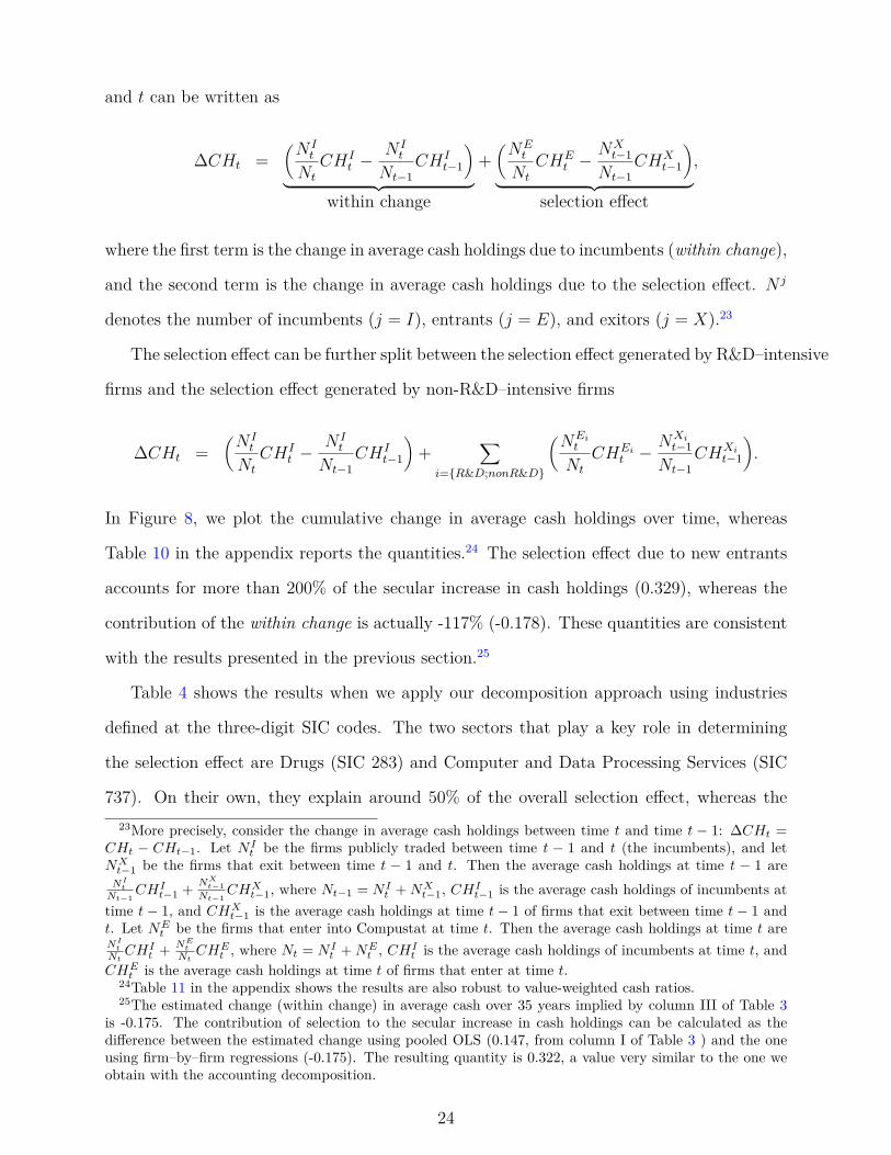
and t can be written as
∆CHt =(N It
Nt
CHIt −
N It
Nt−1CHI
t−1
)︸ ︷︷ ︸
within change
+(NEt
Nt
CHEt −
NXt−1
Nt−1CHX
t−1
)︸ ︷︷ ︸
selection effect
,
where the first term is the change in average cash holdings due to incumbents (within change),
and the second term is the change in average cash holdings due to the selection effect. N j
denotes the number of incumbents (j = I), entrants (j = E), and exitors (j = X).23
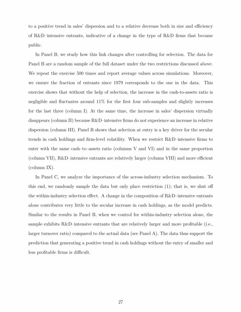
The selection effect can be further split between the selection effect generated by R&D–intensive
firms and the selection effect generated by non-R&D–intensive firms
∆CHt =(N It
Nt
CHIt −
N It
Nt−1CHI
t−1
)+
∑i={R&D;nonR&D}
(NEit
Nt
CHEit −
NXit−1
Nt−1CHXi
t−1
).
In Figure 8, we plot the cumulative change in average cash holdings over time, whereas
Table 10 in the appendix reports the quantities.24 The selection effect due to new entrants
accounts for more than 200% of the secular increase in cash holdings (0.329), whereas the
contribution of the within change is actually -117% (-0.178). These quantities are consistent
with the results presented in the previous section.25
Table 4 shows the results when we apply our decomposition approach using industries
defined at the three-digit SIC codes. The two sectors that play a key role in determining
the selection effect are Drugs (SIC 283) and Computer and Data Processing Services (SIC
737). On their own, they explain around 50% of the overall selection effect, whereas the23More precisely, consider the change in average cash holdings between time t and time t − 1: ∆CHt =
CHt − CHt−1. Let N It be the firms publicly traded between time t − 1 and t (the incumbents), and let
NXt−1 be the firms that exit between time t − 1 and t. Then the average cash holdings at time t − 1 areNI
t
Nt−1CHI
t−1 + NXt−1
Nt−1CHX
t−1, where Nt−1 = N It +NX
t−1, CHIt−1 is the average cash holdings of incumbents at
time t− 1, and CHXt−1 is the average cash holdings at time t− 1 of firms that exit between time t− 1 and
t. Let NEt be the firms that enter into Compustat at time t. Then the average cash holdings at time t are
NIt
NtCHI
t + NEt
NtCHE
t , where Nt = N It +NE
t , CHIt is the average cash holdings of incumbents at time t, and
CHEt is the average cash holdings at time t of firms that enter at time t.
24Table 11 in the appendix shows the results are also robust to value-weighted cash ratios.25The estimated change (within change) in average cash over 35 years implied by column III of Table 3
is -0.175. The contribution of selection to the secular increase in cash holdings can be calculated as thedifference between the estimated change using pooled OLS (0.147, from column I of Table 3 ) and the oneusing firm–by–firm regressions (-0.175). The resulting quantity is 0.322, a value very similar to the one weobtain with the accounting decomposition.
24
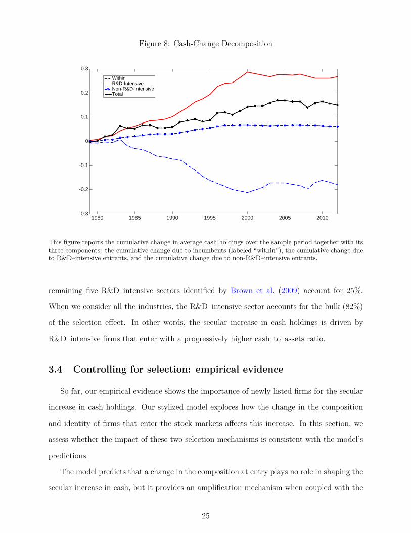
Figure 8: Cash-Change Decomposition
1980 1985 1990 1995 2000 2005 2010-0.3
-0.2
-0.1
0
0.1
0.2
0.3
WithinR&D-IntensiveNon-R&D-IntensiveTotal
This figure reports the cumulative change in average cash holdings over the sample period together with itsthree components: the cumulative change due to incumbents (labeled “within”), the cumulative change dueto R&D–intensive entrants, and the cumulative change due to non-R&D–intensive entrants.
remaining five R&D–intensive sectors identified by Brown et al. (2009) account for 25%.
When we consider all the industries, the R&D–intensive sector accounts for the bulk (82%)
of the selection effect. In other words, the secular increase in cash holdings is driven by
R&D–intensive firms that enter with a progressively higher cash–to–assets ratio.
3.4 Controlling for selection: empirical evidence
So far, our empirical evidence shows the importance of newly listed firms for the secular
increase in cash holdings. Our stylized model explores how the change in the composition
and identity of firms that enter the stock markets affects this increase. In this section, we
assess whether the impact of these two selection mechanisms is consistent with the model’s
predictions.
The model predicts that a change in the composition at entry plays no role in shaping the
secular increase in cash, but it provides an amplification mechanism when coupled with the
25
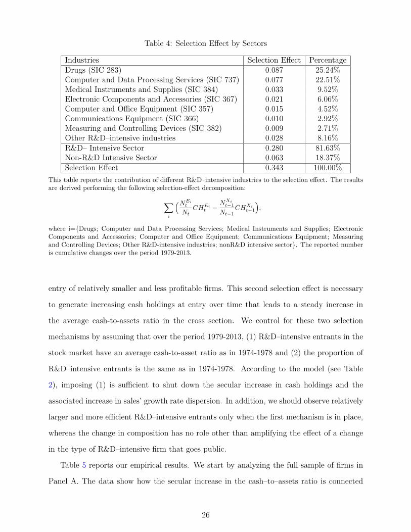
Table 4: Selection Effect by Sectors
Industries Selection Effect PercentageDrugs (SIC 283) 0.087 25.24%Computer and Data Processing Services (SIC 737) 0.077 22.51%Medical Instruments and Supplies (SIC 384) 0.033 9.52%Electronic Components and Accessories (SIC 367) 0.021 6.06%Computer and Office Equipment (SIC 357) 0.015 4.52%Communications Equipment (SIC 366) 0.010 2.92%Measuring and Controlling Devices (SIC 382) 0.009 2.71%Other R&D–intensive industries 0.028 8.16%R&D– Intensive Sector 0.280 81.63%Non-R&D Intensive Sector 0.063 18.37%Selection Effect 0.343 100.00%
This table reports the contribution of different R&D–intensive industries to the selection effect. The resultsare derived performing the following selection-effect decomposition:
∑i
(NEit
NtCHEi
t −NXit−1
Nt−1CHXi
t−1
),
where i={Drugs; Computer and Data Processing Services; Medical Instruments and Supplies; ElectronicComponents and Accessories; Computer and Office Equipment; Communications Equipment; Measuringand Controlling Devices; Other R&D-intensive industries; nonR&D intensive sector}. The reported numberis cumulative changes over the period 1979-2013.
entry of relatively smaller and less profitable firms. This second selection effect is necessary
to generate increasing cash holdings at entry over time that leads to a steady increase in
the average cash-to-assets ratio in the cross section. We control for these two selection
mechanisms by assuming that over the period 1979-2013, (1) R&D–intensive entrants in the
stock market have an average cash-to-asset ratio as in 1974-1978 and (2) the proportion of
R&D–intensive entrants is the same as in 1974-1978. According to the model (see Table
2), imposing (1) is sufficient to shut down the secular increase in cash holdings and the
associated increase in sales’ growth rate dispersion. In addition, we should observe relatively
larger and more efficient R&D–intensive entrants only when the first mechanism is in place,
whereas the change in composition has no role other than amplifying the effect of a change
in the type of R&D–intensive firm that goes public.
Table 5 reports our empirical results. We start by analyzing the full sample of firms in
Panel A. The data show how the secular increase in the cash–to–assets ratio is connected
26
to a positive trend in sales’ dispersion and to a relative decrease both in size and efficiency
of R&D–intensive entrants, indicative of a change in the type of R&D firms that became
public.
In Panel B, we study how this link changes after controlling for selection. The data for
Panel B are a random sample of the full dataset under the two restrictions discussed above.
We repeat the exercise 500 times and report average values across simulations. Moreover,
we ensure the fraction of entrants since 1979 corresponds to the one in the data. This
exercise shows that without the help of selection, the increase in the cash-to-assets ratio is
negligible and fluctuates around 11% for the first four sub-samples and slightly increases
for the last three (column I). At the same time, the increase in sales’ dispersion virtually
disappears (column II) because R&D–intensive firms do not experience an increase in relative
dispersion (column III). Panel B shows that selection at entry is a key driver for the secular
trends in cash holdings and firm-level volatility. When we restrict R&D–intensive firms to
enter with the same cash–to–assets ratio (columns V and VI) and in the same proportion
(column VII), R&D–intensive entrants are relatively larger (column VIII) and more efficient
(column IX).
In Panel C, we analyze the importance of the across-industry selection mechanism. To
this end, we randomly sample the data but only place restriction (1); that is, we shut off
the within-industry selection effect. A change in the composition of R&D–intensive entrants
alone contributes very little to the secular increase in cash holdings, as the model predicts.
Similar to the results in Panel B, when we control for within-industry selection alone, the
sample exhibits R&D–intensive entrants that are relatively larger and more profitable (i.e.,
larger turnover ratio) compared to the actual data (see Panel A). The data thus support the
prediction that generating a positive trend in cash holdings without the entry of smaller and
less profitable firms is difficult.
27
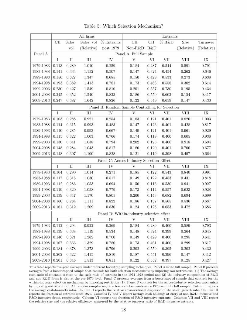
Table 5: Which Selection Mechanism?
All firms EntrantsCH Sales’ Sales’ vol % Entrants CH CH % R&D Size Turnover
vol (Relative) post 1979 Non-R&D R&D (Relative) (Relative)Panel A Panel A: Full Sample
I II III IV V VI VII VIII IX1979-1983 0.113 0.289 1.010 0.259 0.184 0.287 0.544 0.591 0.7911983-1988 0.141 0.334 1.152 0.507 0.147 0.324 0.454 0.262 0.6461989-1993 0.156 0.327 1.347 0.685 0.150 0.429 0.533 0.273 0.6381994-1998 0.193 0.382 1.413 0.781 0.173 0.463 0.558 0.302 0.6141999-2003 0.230 0.427 1.549 0.810 0.201 0.557 0.730 0.195 0.4342004-2008 0.245 0.352 1.540 0.823 0.186 0.550 0.603 0.154 0.4172009-2013 0.247 0.387 1.642 0.826 0.122 0.549 0.659 0.147 0.430
Panel B: Random Sample Controlling for SelectionI II III IV V VI VII VIII IX
1979-1983 0.103 0.288 0.921 0.254 0.183 0.121 0.401 0.826 1.0031983-1988 0.114 0.315 0.993 0.483 0.147 0.123 0.401 0.428 0.8171989-1993 0.110 0.285 0.993 0.667 0.149 0.121 0.401 0.961 0.9291994-1998 0.115 0.322 1.003 0.766 0.174 0.119 0.400 0.605 0.9381999-2003 0.130 0.341 1.038 0.794 0.202 0.125 0.400 0.918 0.6942004-2008 0.148 0.284 1.043 0.817 0.186 0.120 0.401 0.700 0.6772009-2013 0.148 0.307 1.100 0.828 0.121 0.119 0.398 0.497 0.664
Panel C: Across-Industry Selection EffectI II III IV V VI VII VIII IX
1979-1983 0.104 0.290 1.014 0.271 0.185 0.122 0.543 0.840 0.9911983-1988 0.117 0.315 1.030 0.517 0.149 0.122 0.453 0.431 0.8181989-1993 0.112 0.286 1.053 0.694 0.150 0.116 0.530 0.941 0.9271994-1998 0.119 0.320 1.058 0.779 0.173 0.114 0.557 0.623 0.9281999-2003 0.139 0.347 1.170 0.805 0.200 0.143 0.682 0.694 0.6992004-2008 0.160 0.284 1.111 0.822 0.186 0.137 0.565 0.536 0.6872009-2013 0.161 0.312 1.209 0.830 0.124 0.126 0.653 0.472 0.686
Panel D: Within-industry selection effectI II III IV V VI VII VIII IX
1979-1983 0.112 0.294 0.922 0.269 0.184 0.289 0.400 0.589 0.7931983-1988 0.139 0.338 1.119 0.534 0.148 0.324 0.399 0.264 0.6451989-1993 0.146 0.321 1.282 0.700 0.149 0.429 0.400 0.295 0.6411994-1998 0.167 0.363 1.329 0.780 0.173 0.461 0.400 0.299 0.6171999-2003 0.184 0.378 1.373 0.796 0.202 0.559 0.395 0.202 0.4322004-2008 0.202 0.322 1.415 0.810 0.187 0.551 0.396 0.147 0.4122009-2013 0.201 0.346 1.513 0.811 0.122 0.552 0.397 0.125 0.427
This table reports five-year averages under different bootstrap sampling techniques. Panel A is the full sample. Panel B presentsaverages from a bootstrapped sample that controls for both selection mechanisms by imposing two restrictions: (1) The averagecash ratio of entrants is close to the cash ratio of entrants in the 1974-1978 period and (2) the industry composition of R&Dand non-R&D firms is also at the pre-1979 level. Panel C presents averages from a bootstrapped sample that controls for thewithin-industry selection mechanism by imposing restriction (1). Panel D controls for the across-industry selection mechanismby imposing restriction (2). All random samples keep the fraction of entrants since 1978 as in the full sample. Column I reportsthe average cash-to-assets ratio. Column II reports the relative cross-sectional disperson of the sales’ growth rate. Column IIIreports the fraction of entrants since 1979. Columns IV and V report average cash holdings at entry of non-R&D-intensive andR&D-intensive firms, respectively. Column VI reports the fraction of R&D-intensive entrants. Columns VII and VIII reportthe relative size and the relative efficiency, measured by the relative turnover ratio of R&D-intensive entrants.
28
In Panel D, we shut off the across-industry selection mechanism and turn on the intra-
industry selection mechanism by randomly sampling the data from the full sample but keep-
ing the proportion of R&D–intensive entrants to non-R&D–intensive entrants constant. The
increase in the cash-to-assets ratio is quite large, and the relative size and efficiency are
falling, as the model predicts. At the same time, without the amplification effect provided
by the compositional change, the intra-industry selection mechanism cannot explain the
entire change in the average cash-to-assets ratio.
3.5 What determines the cash ratio at entry?
The results in the previous section highlight a tight connection between the cash-to-
assets ratio at entry for R&D–intensive firms and our proxy for firm-level efficiency (i.e., the
turnover ratio). In this section, we compare the explanatory power of the latter variable
with other important determinants of corporate cash holdings.
First we show in Figure 9 firms’ average cash holdings for each cohort of entrants around
the IPO year. For both sectors, average cash holdings are smaller before the IPO year and de-
crease the year after the IPO below their pre–IPO values.26 However, only the R&D–intensive
sector (left panel) shows a secular trend in average cash holdings before the IPO year, a phe-
nomenon that clearly does not depend on a higher retention of IPO proceeds.
Table 6 studies what determines the cash–to–assets ratio entry by focusing on quantities
in the fiscal year that precede the IPO year. We consider widely studied determinants in
the cash holding literature (e.g., Azar et al. (2016) and Bates et al. (2009)) and include the
turnover ratio as a proxy for the underlying total revenue productivity shock, as suggested
by the model. In column I, we consider all variables. Only the T-bill rate does not enter
significantly.27 In column II, we report the Shapley-Owen’s R-square decomposition (Israeli
(2007) and Huettner and Sunder (2012)) to measure each individual independent variable’s26We can perform these calculations because Compustat reports up to three years of firms’ accounting
data prior to their IPO.27Following Azar et al. (2016), we include the T-bill as a main predictor of corporate cash holdings. Unlike
Azar et al. (2016), we cannot compute the cost of carry cash at the individual firm level given the lack ofobservations in the years preceding the IPO.
29
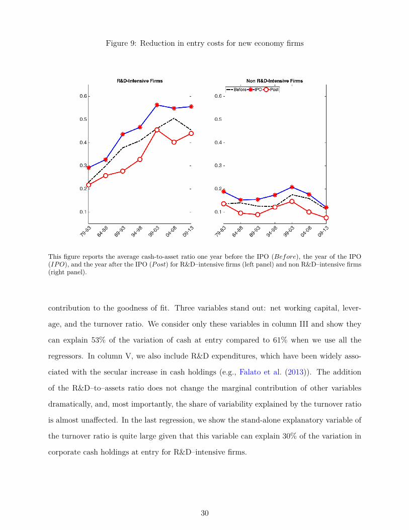
Figure 9: Reduction in entry costs for new economy firms
This figure reports the average cash-to-asset ratio one year before the IPO (Before), the year of the IPO(IPO), and the year after the IPO (Post) for R&D–intensive firms (left panel) and non R&D–intensive firms(right panel).
contribution to the goodness of fit. Three variables stand out: net working capital, lever-
age, and the turnover ratio. We consider only these variables in column III and show they
can explain 53% of the variation of cash at entry compared to 61% when we use all the
regressors. In column V, we also include R&D expenditures, which have been widely asso-
ciated with the secular increase in cash holdings (e.g., Falato et al. (2013)). The addition
of the R&D–to–assets ratio does not change the marginal contribution of other variables
dramatically, and, most importantly, the share of variability explained by the turnover ratio
is almost unaffected. In the last regression, we show the stand-alone explanatory variable of
the turnover ratio is quite large given that this variable can explain 30% of the variation in
corporate cash holdings at entry for R&D–intensive firms.
30

Table 6: What drives the cash ratio?
VARIABLES CH %R2 CH %R2 CH %R2 CHI II III IV V VI VII
Tbill (3-Month) -0.137 2.418(0.160)
Size -0.019*** 1.925(0.003)
Cash Flows 0.066*** 4.829(0.016)
NWC -0.323*** 12.64 -0.373*** 22.230 -0.318*** 17.889(0.021) (0.019) (0.019)
R&D 0.210*** 8.633 0.168*** 11.370(0.027) (0.019)
Dividend -0.047*** 2.117(0.016)
Market / Book 0.001 1.337(0.001)
CAPEX -0.606*** 5.200(0.055)
Leverage -0.630*** 27.933 -0.757*** 38.907 -0.733*** 36.128(0.024) (0.023) (0.023)
Acquisition -0.643*** 4.802(0.060)
Turnover -0.167*** 28.168 -0.168*** 38.864 -0.160*** 34.614 -0.243***(0.007) (0.006) (0.006) (0.07)
Constant 0.658*** 0.650*** 0.611*** 0.599***(0.011) (0.006) (0.008) (0.07)
Observations 2,314 2,773 2,773 2,923R-squared 0.610 0.530 0.543 0.296
This table reports cross-sectional regressions where the dependent variable is the cash-to-assets ratio (Com-pustat item che divided by at) in the fiscal year before a company goes public. We only consider firms inthe R&D-intensive sector. The independent variables are Size (log of real total assets, Compustat item at),Cash Flows ((oibdp - xint - dvc - txt)/at)), Net Working Capital ((wcap-che)/at), R&D over sales (xrd/sale,we set xrd to zero when missing); Dividend Dummy (takes the value of 1 if dvc > 0 and zero otherwise),Market-to-Book ratio ((at+prcc f*csho-ceq)/at), Capital expenditures (capx/at), Leverage ((dltt+dlc)/at);Acquisition (aqc/at), and Turnover ratio (sale/at). ”Observations” reports the number of R&D-intensivefirms for which we have observations on accounting quantities in the fiscal year before the IPO. For eachof the first three regressions, we report the contribution of each individual independent variable using theShapley-Owen decomposition (Huettner and Sunder (2012)). For the regression in column VII, the Shapley-Owen decomposition delivers a value of 100 and we do not report it. We report robust standard errors. *denotes significance at the 10% level, ** denotes significance at the 5% level, and *** denotes significanceat the 1% level.
31
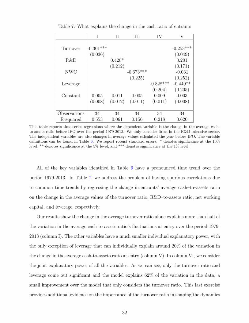
Table 7: What explains the change in the cash ratio of entrants
I II III IV V
Turnover -0.301*** -0.253***(0.036) (0.049)
R&D 0.420* 0.201(0.212) (0.171)
NWC -0.673*** -0.031(0.225) (0.252)
Leverage -0.828*** -0.449**(0.204) (0.205)
Constant 0.005 0.011 0.005 0.009 0.003(0.008) (0.012) (0.011) (0.011) (0.008)
Observations 34 34 34 34 34R-squared 0.553 0.061 0.156 0.218 0.620
This table reports time-series regressions where the dependent variable is the change in the average cash-to-assets ratio before IPO over the period 1979-2013. We only consider firms in the R&D-intensive sector.The independent variables are also changes in average values calculated the year before IPO. The variabledefinitions can be found in Table 6. We report robust standard errors. * denotes significance at the 10%level, ** denotes significance at the 5% level, and *** denotes significance at the 1% level.
All of the key variables identified in Table 6 have a pronounced time trend over the
period 1979-2013. In Table 7, we address the problem of having spurious correlations due
to common time trends by regressing the change in entrants’ average cash–to–assets ratio
on the change in the average values of the turnover ratio, R&D–to-assets ratio, net working
capital, and leverage, respectively.
Our results show the change in the average turnover ratio alone explains more than half of
the variation in the average cash-to-assets ratio’s fluctuations at entry over the period 1979-
2013 (column I). The other variables have a much smaller individual explanatory power, with
the only exception of leverage that can individually explain around 20% of the variation in
the change in the average cash-to-assets ratio at entry (column V). In column VI, we consider
the joint explanatory power of all the variables. As we can see, only the turnover ratio and
leverage come out significant and the model explains 62% of the variation in the data, a
small improvement over the model that only considers the turnover ratio. This last exercise
provides additional evidence on the importance of the turnover ratio in shaping the dynamics
32
of the average cash-to-assets ratio over the last 35 years.
4 Conclusion
This paper finds that sample selection has been a key driver of the increase in the average
cash–to–assets ratio for U.S. public companies over the last 35 years. While new entrants to
the stock market have increased their cash–to–assets ratios, the typical U.S. public company
experiences a decline in cash holdings over time. The selection effect is powerful enough to
reverse the negative within-firm effect and to generate a secular increase.
A stylized firm industry model with endogenous entry allows us to study how selection
mechanisms can shape the average cash–to–assets ratio. More than a shift in the composition
of R&D–intensive firms, a shift toward smaller, initially less productive, but higher-growth-
potential firms is the key driver of higher cash balances at IPO. This mechanisms is backed
up by the data as we show with bootstrap sampling techniques. The data also show the
turnover ratio, as a proxy for firm-level productivity, is a key predictor for cash ratios at
entry, as our model suggests.
All in all, our results suggest a new direction in the debate about the causes of the secular
increase in the corporate cash–to–assets ratio and other observed changes in investment and
financing practices. Instead of focusing on factors that influence incumbents’ investment
and financing decisions, we advocate for a shift of research efforts toward understanding why
more R&D–intensive firms go public and why they do so with higher cash–to–assets ratios
over time.
33
REFERENCES
Anderson, R. W. and A. Carverhill (2012). Corporate liquidity and capital structure. Review of
Financial Studies 25 (3), 797–837.
Armenter, R. and V. Hnatkovska (2016). Technical report, Working Paper.
Asker, J., J. Farre-Mensa, and A. Ljungqvist (2014). Corporate investment and stock market
listing: a puzzle? Review of Financial Studies.
Azar, J., J.-F. Kagy, and M. C. Schmalz (2016). Can changes in the cost of carry explain the
dynamics of corporate cash holdings? Review of Financial Studies, Forthcoming.
Baker, M. and J. Wurgler (2004). Appearing and disappearing dividends: The link to catering
incentives. Journal of Financial Economics 73, 271–288.
Banerjee, S., V. A. Gatchev, and P. A. Spindt (2007). Stock market liquidity and firm dividend
policy. Journal of Financial and Quantitative Analysis 42, 369–398.
Bargeron, L. L., K. M. Lehn, and C. J. Zutter (2010). Sarbanes–oxley and corporate risk–taking.
Journal of Accounting and Economics 49, 34–52.
Bates, T. W., K. M. Kahle, and R. Stulz (2009). Why do us firms hold so much more cash than
they used to? Journal of Finance 64 (5), 1985–2021.
Baumol, W. J. (1952). The transactions demand for cash: An inventory theoretic approach. Quar-
terly Journal of Economics 66 (4), 545–556.
Begenau, J. and J. Salomao (2016). Firm financing over the business cycle. Working Paper .
Booth, L. and J. Zhou (2013). Increase in cash holdings: Pervasive or sector-specific? Frontiers in
Finance and Economics 10 (2), 31–62.
Brown, G. and N. Kapadia (2007). Firm-specific risk and equity market development. Journal of
Financial Economics 84 (2), 358–388.
Brown, J., S. M. Fazzari, and B. C. Petersen (2009). Financing innovation and growth: Cash flow,
external equity, and the 1990s r&d boom. Journal of Finance 54 (1), 151–185.
34
Brown, J. R. and B. C. Petersen (2011). Cash holdings and r&d smoothing. Journal of Corporate
Finance 17, 2011.
Buera, F. J. and J. P. Kaboski (2012). The rise of the service economy. American Economic
Review 6 (102), 2540–2569.
Butters, J. K. (1949). Federal income taxation and external vs. internal financing. The Journal of
Finance 4 (3), 197–205.
Chemmanur, Thomas J Krishnan, K. and Q. Yu (2016). Venture capital backing, investor attention,
and initial public offerings. Working Paper .
Chen, P., L. Karabarbounis, and B. Neiman (2017). The global rise of corporate savings. NBER
Working Paper 23133 .
Clementi, G. L. (2002). Ipos and the growth of firms. Working Paper .
Clementi, G. L. and B. Palazzo (2016). Entry, exit, firm dynamics, and aggregate fluctuations.
American Economic Journal: Macroeconomics 8 (3), 1–41.
Curtis, C., J. Garin, and M. S. Mehkari (2015). Inflation and the evolution of firm-level liquid
assets. Technical report.
Davis, S. J., J. Haltiwanger, R. Jarmin, and J. Miranda (2007). Volatility and dispersion in
business growth rates: Publicly traded versus privately held firms. In NBER Macroeconomics
Annual 2006, Volume 21, pp. 107–180. MIT Press.
Dittmar, A. and J. Mahrt-Smith (2007). Corporate governance and the value of cash holdings.
Journal of Financial Economics 83 (3), 599–634.
Evans, D. S. (1987). The relationship between firm growth, size, and age: Estimates for 100
manufacturing industries. Journal of Industrial Economics 35 (4), 567–581.
Falato, A., D. Kadyrzhanova, and J. Sim (2013). Rising intangible capital, shrinking debt capacity,
and the us corporate savings glut.
35

Falato, A. and J. Sim (2014). Why do innovative firms hold so much cash? evidence from changes
in state r&d tax credits. Technical report, Federal Reserve Board, Washington, D.C., Federal
Reserve Board, Washington, D.C.
Fama, E. F. and K. R. French (2001). Disappearing dividends: changing firm characteristics or
lower propensity to pay? Journal of Financial economics 60 (1), 3–43.
Fama, E. F. and K. R. French (2004). New lists: Fundamentals and survival rates. Journal of
Finance 73 (2), 229–269.
Farre-Mensa, J. (2014). Comparing the cash policies of public and private firms.
Faulkender, M. and M. Petersen (2012). Investment and capital constraints: Repatriations under
the american jobs creation act. Review of Financial Studies 25 (11), 3351–3388.
Foley, F. C., J. C. Hartzell, S. Titman, and G. Twite (2007). Why do firms hold so much cash? a
tax–based explanation. Journal of Financial Economics 86, 579–607.
Froot, K. A., D. S. Scharfstein, and J. C. Stein (1993). Risk management: Coordinating corporate
investment and financing policies. Journal of Finance 48 (5), 1629–1658.
Gamba, A. and A. Triantis (2008). The value of financial flexibility. Journal of Finance 63 (5),
2263–2296.
Gao, X. (2015). Corporate cash hoarding: The role of just-in-time adoption. Technical report,
UBC Working Paper.
Graham, J. and M. Leary (2016). The evolution of corporate cash. Working Paper .
Hall, B. H. (2007). Measuring the returns to r&d: The depreciation problem. NBER Working
Paper 13473 .
Haltiwanger, J., I. Hathaway, and J. Miranda (2014). Declining business dynamism in the u.s.
high-technology sector. Kaufmann Foundation Working Paper .
Hartzell, J., S. Titman, and G. Twite (2005). Why do firms hold so much cash? a tax-based
explanation. Journal of Financial Economics.
36
He, Z. and M. B. Wintoki (2014). The cost of innovation: R&d and high cash holdings in u.s. firms.
Heckman, J. J. (1979). Sample selection bias as a specification error. Econometrica: Journal of the
Econometric Society, 153–161.
Hennessy, C. A. and T. M. Whited (2007). How costly is external financing? evidence from a
structural estimation. Journal of Finance 62 (4), 1705–1745.
Hines, J. R. and E. M. Rice (1994). Fiscal paradise: Foreign tax havens and american business.
The Quarterly Journal of Economics 109 (1), 149–82.
Hoberg, G. and N. R. Prabhala (2009). Disappearing dividends, catering, and risk. Review of
Financial Studies 22 (1), 79–116.
Hopenhayn, H. A. (1992). Entry, exit, and firm dynamics in long run equilibrium. Econometrica:
Journal of the Econometric Society, 1127–1150.
Huettner, F. and M. Sunder (2012). Axiomatic arguments for decomposing goodness of fit according
to shapley and owen values. Electronic Journal of Statistics 6, 1239–1250.
Israeli, O. (2007). A shapley-based decomposition of the r-square of a linear regression. Journal of
Economic Inequality 5.
Jensen, M. C. (1986). Agency costs of free cash flow, corporate finance, and takeovers. American
Economic Review 76 (2), 323–329.
Jovanovic, B. and P. Rousseau (2001). Why wait? a century of life before ipo. American Economic
Review 91 (2), 336–341.
Kim, C.-S., D. C. Mauer, and A. E. Sherman (1998). The determinants of corporate liquidity:
Theory and evidence. Journal of financial and quantitative analysis 33 (03), 335–359.
Klette, T. J. and S. Kortum (2004). Innovating firms and aggregate innovation. Journal of Political
Economy 112 (5), 986–1018.
Lemmon, M. L., M. R. Roberts, and J. F. Zender (2008). Back to the beginning: Persistence and
the cross-section of corporate capital structure. Journal of Finance 63 (4), 1575–1608.
37
Li, W. C. Y. (2012). Depreciation of business r&d capital. Technical report, U.S. Bureau of
Economic Analysis.
Longstreth, B. (1987). Modern Investment Management and the Prudent Man Rule. Oxford Uni-
versity Press.
Loughran, T. and J. R. Ritter (2004). Why has ipo underpricing changed over time? Financial
Management 33 (3).
Lyandres, E. and B. Palazzo (2015). Cash holdings, competition, and innovation. Journal of
Financial and Quantitative Analysis, Forthcoming.
Malamud, S. and F. Zucchi (2016). Liquidity, innovation, and endogenous growth. Working Paper .
McLean, R. D. (2011). Share issuance and cash savings. Journal of Financial Economics 99,
693–715.
Michelacci, C. and J. Suarez (2004). Business creation and the stock market. The Review of
Economic Studies 71 (2), 459–481.
Miller, M. H. and D. Orr (1966). A model of the demand for money by firms. Quarterly Journal
of Economics 80 (3), 413–435.
Nikolov, B. and T. Whited (2014). Agency conflicts and cash: Estimates from a dynamic model.
Journal of Finance 69 (5), 1883–1921.
Officer, M. S. (2011). Overinvestment, corporate governance, and dividend initiations. Journal of
Corporate Finance 17, 710–724.
Opler, T., L. Pinkowitz, R. Stulz, and R. Williamson (1999). The determinants and implications
of corporate cash holdings. Journal of Financial Economics 52, 3–46.
Opler, T. and S. Titman (1994). Financial distress and corporate performance. Journal of Fi-
nance 49 (3), 1015–1040.
Pinkowitz, L., R. M. Stulz, and R. Williamson (2016). Do us firms hold more cash than foreign
firms do? Review of Financial Studies 29 (2), 309–348.
38
Riddick, L. A. and T. M. Whited (2009). The corporate propensity to save. The Journal of
Finance 64 (4), 1729–1766.
Roberts, M. R. and T. M. Whited (2013). Endogeneity in empirical corporate finance. Handbook
of the Economics of Finance 2, 493–572.
Rouwenhorst, K. G. (1995). Asset pricing implications of equilibrium business cycle models. In
T. Cooley (Ed.), Frontiers of Business Cycle Research, pp. 294–330. Princeton University Press.
Tobin, J. (1956). The interest–elasticity of transactions demand for cash. The Review of Economics
and Statistics 38 (3), 241–247.
Vogel, R. C. and G. Maddala (1967). Cross-section estimates of liquid asset demand by manufac-
turing corporations. The Journal of Finance 22 (4), 557–575.
Warusawitharana, M. (2015). Research and development, profits, and firm value: A structural
estimation. Quantitative Economics 6 (2), 531–565.
Zhao, J. (2015). Accounting for the corporate cash increase. Available at SSRN 2492339 .
39
A On the Model
This appendix section presents the details of the model presented in section 2.
A.1 Firm industry equilibrium
Denote ω as the fraction of old-economy firms. Given ω and the riskless rate R, a
recursive competitive equilibrium consists of (i) value functions V i (ki, si,z) and V E,i(q),
(ii) policy functions l′i (ki, si,z) and x′i (ki, si,z) , and (iii) bounded sequences of incumbents’
measure {Γit}∞t=1 and entrants’ measures {εit}
∞t=0 ∀i ∈ {o, n} such that
1. V i (ki, si,z), l′i (ki, si,z), and x′i (ki, si,z) solve the incumbents problem ∀i ∈ {o, n} .
2. V E,i (q), s′i (q) and x′i (q) solve the entrants problem ∀i ∈ {o, n} .
3. For all Borel sets Z ×K × L×X ×< and ∀t ≥ 0 and W = K × L
εit+1(W ) = Mi
∫Z
∫BEi (W )
dQ(q)d(F (z′∗|q)).
where BEi(W ) ={
(s′i(q), x′i(q)) s.t. l′i(q) ∈ L, x′i (q) ∈ Xand V E,i ≥ ce,i}
denotes the
policy functions of entrants.
4. For all Borel sets Z ×K × L×X ×< and ∀t ≥ 0 and W = K × L ,
Γit+1(W ′) = (1− φ)∫Z
∫Bi(W )
dΓit(W )dF (z′|z) + εit+1(W ),
whereBi(W ) denotes the policy functions of incumbents and ω = Γot+1(W ′)/(Γnt+1(W ′)+
Γot+1(W ′)).
The distribution of firms evolves in the following way. A mass of entrants receives a signal
and some decide to enter. The signal q determines the productivity level of the following
period. Firms choose savings and capital investment. These choices determine the expected
net worth for the following period. Conditional on not exiting, incumbent firms pick the
period’s investment, internal, or external funds. The shocks follow a Markov distribution.
40
A.2 Parametrization
We parametrize the model at an annual frequency using calibrated parameters that match
key features of U.S. public companies. To highlight the role of selection, we calibrate the
parameters using the period 1959-1979, i.e. before the large increase in cash–holdings.
A few standard parameters are set to values used in the literature. Following Hennessy
and Whited (2007), we set the decreasing returns-to-scale parameter to 0.62 and the depreci-
ation rate to 0.15. Following Riddick and Whited (2009), we set the annual risk-free interest
rate to 4% and the conditional standard deviation of the idiosyncratic shock to 0.121. Table
1 reports the parameter values and their targets.
We calibrate the remaining parameters to match key moments, using data from the period
1959–1979. The proportion of potential entrants of type old (ω) is set to 0.668. This value
allows us to replicate the composition of publicly traded firms during the period 1959-1979.
We set the persistence parameter equal to 0.90 – a value within the estimates provided by
Hennessy and Whited (2007) – to match the standard deviation of the sales’ growth rate
during the period 1959-1979. We define the latter quantity as ∆yt = yt−yt−10.5yt−1+0.5yt−1
.
Then we calibrate a set of parameters to replicate key cash holdings moments for publicly
traded firms in 1979. First, we calibrate the cost of carrying cash inside the firm, ν, to match
the average cash–to–assets ratio. Second, we choose a number for the value of staying private
to match the average cash–to–assets ratio at entry. The proportional equity issuance cost
(κ) is set to match the average equity-to-assets ratio over the period 1959-1979. We define
the cash–to–assets ratio in the model as cash holdings divided by the beginning of the period
capital plus cash holdings, whereas the equity–to–assets ratio as equity issuance divided by
the beginning of the period capital plus cash holdings.
The parameter that governs the investment adjustment cost is set to deliver an investment-
rate standard deviation close to the one found in the data over the period 1959-1979.28
The parameter that governs the shape of the Pareto distribution, ξ, over the set of signals
is chosen to match the size of entrants relative to the size of incumbents of age 5. We measure28We measure the investment rate in the data as capital expenditures (Compustat item capx) divided by
the previous period value of net property, plant, and equipment (item ppent).
41
firm size using total sales.29 Panel B of Table 1 reports the simulated moments together with
their empirical counterpart.
To conclude, we set the exogenous exit rate (λ) to 7%, a value that delivers an age
(i.e., years since entry) distribution close to the age distribution in Compustat over the
period 1979-2013 (Panel C of Table 1). In our model (as in the data), the years since entry
distribution matters because firms that recently IPOed tend to be smaller and have larger
cash–to–assets ratios. For this reason, we choose an exit rate that delivers an age distribution
as close as possible to the data.
Solution
We solve the incumbent problem by value function iteration. We discretize the firm-level
shock with 35 grid points using the method in Rouwenhorst (1995). We discretize the capital
grid using 200 grid points, the net leverage grid for old-economy firms using 100 grid points,
and the cash grid for new-economy firms using 100 grid points. We also scale the revenue
function so that the capital choice is between zero and 1.
We also solve the entrant problem by value function iteration. We discretize the signal
space using 100 grid points. The lower (upper) bound of the signal grid coincides with the
lower (upper) bound of the firm-level shock grid. We use a discrete version of the Pareto
distribution to allocate the mass of potential entrants over the signal space.
A.3 Incumbent policy functions
Figure 10 illustrates the policy functions for an incumbent firm as a function of the
firm–level shock. The top panels are policies for two firms that have the same size, as
measured by their beginning of the period capital, and only differ in their beginning of the
period cash balances. The left panel shows these two firms choose the same capital next
period if they are both distributing dividends or issuing equity. For small values of the
shock, both firms have the same investment and financing policies. In particular, when the29We assume Q(q) = 1− (q/q)ξ, ξ > 1, where q is the lower bound of the signal grid. For further details,
see Appendix B in Clementi and Palazzo (2016).
42

Figure 10: Policy Functions
-1 0 1 20
0.02
0.04
0.06
0.08
0.1Capital next Period
Low CashHigh Cash
-1 0 1 2-0.06
-0.04
-0.02
0
0.02
0.04
0.06Dividend
-1 0 1 20
0.002
0.004
0.006
0.008
0.01
0.012Cash next Period
-1 0 1 20
0.02
0.04
0.06
0.08
0.1Capital next Period
High CapitalLow Capital
-1 0 1 2-0.06
-0.04
-0.02
0
0.02
0.04Dividend
-1 0 1 2
#10-3
0
2
4
6
8Cash next Period
The figure reports the policy functions as a function of the firm-level shock for a new-economy firm. The leftpanels depict the optimal capital choice, the middle panels depict the distributed dividends, and the rightpanels depict the optimal saving policy. The top panels report the policies for a high-cash firm (red line) anda low-cash firm (blue line), while considering the same level of beginning-of-the-period capital stock. Thebottom panels report the policies for a low-capital firm (red line) and a high-capital firm (blue line), whileconsidering the same level of beginning-of-the-period cash.
productivity shock is very low, both firms find it more convenient to distribute dividends
rather than to invest. As the productivity increases (i.e., the shock becomes larger), in order
to take advantage of a good state, both firms decide to reduce their dividend distributions
and to invest more. If the shock becomes large enough, firms save precautionarily. Because
issuing equity is costly, firms save internal resources to avoid equity issues in the near future;
that is, they seek a reduction in their external financing costs. If the shock is very large,
it becomes optimal to stop saving and to issue equity to finance a larger investment. In
the latter case, both firms have similar investment policies, but the firm with less cash has
to issue more costly equity and invest slightly less compared to the firm with larger cash
43
holdings. The difference in equity issuance is exactly equal to the cash balance differential
multiplied by 1 +κ (i.e. 1+ equity issuance cost). To summarize, the three panels show that
cash-rich firms have a larger amount of internal resources that allows them to (i) distribute
more dividends when they are financially unconstrained, (ii) invest more and save more when
financing constraints are binding, and (iii) reduce their financing cost when they decide to
invest in excess of their internal resources, everything else being equal.
Capital is an endogenous state variable because of capital adjustment costs. The bottom
panels of Figure 10 show the policies for two firms that only differ in their beginning-of-
period capital stock (i.e., size). The patterns of the investment and financing policies are very
similar to the ones in the top panels. What emerges from these patterns is the importance
of precautionary financing for small firms. The bottom panels show that large firms have
a smaller precautionary savings motive because they rely on larger expected cash flows,
and for this reason they need to retain less cash when financing constraints are binding.
Conversely, small firms engage in larger precautionary savings, and in doing so they deliver
a larger cash-to-assets ratio given (i) their larger amount of savings and (ii) their smaller
beginning-of-the-period capital.
Simulation
We simulate a panel of 40,000 firms for 300 periods to let the economy settle in the ergodic
state. At each time t, a fraction λ of firms exits the economy. These firms are replaced by
an equal mass of entrants in each period. We discard the first 100 periods and calibrate the
model using the remaining 200.
To run our experiments, we start from the stationary distribution and simulate our
economy for an additional 35 years. We repeat the simulation 200 times and report average
values across the 200 simulations.
44
B Supplemental Empirical Results
In this appendix, we provide graphs and tables to supplement the empirical analysis in
the main body of the paper. All figures and tables are at the end of the document.
The secular increase in cash. Figure 11 shows the average cash–to–assets ratio for U.S.
public companies over the period 1958–2013. What has been dubbed as the secular increase
(Bates et al. (2009)) starts in 1979. In the period 1979–2013, the average cash-holdings value
goes from 0.08 in 1979 to 0.25 in 2013.
Which Cohorts Drove up the Cash–to–Assets Ratio? Given the persistence of cash
balances documented in Table 3, we follow Brown and Kapadia (2007) and estimate a model
that includes a cohort fixed effect using firms that become public from 1959 onward. The
results are reported in Table 9.
When we include cohort fixed effects, the positive trend in column I becomes not signifi-
cant. In column II, the estimates of the cohort fixed effects are differences from the excluded
cohort (1974–1978), whose estimated value is given by the intercept. Column II makes clear
that no differences exist in cohort fixed effects prior to the 1979-1983 cohort, whereas starting
with the latter cohort, the fixed effect becomes significantly bigger and its evolution mimics
the evolution of the average cash holdings at entry depicted in Figure 1. In columns III and
IV, we separately estimate cohort fixed effects for R&D–intensive and non–R&D–intensive
firms. In both cases, no significant differences exist in cohort fixed effects among the first four
cohorts, thus supporting the evidence in Figure 2 that places the beginning of the secular
increase in cash holdings with the 1979–1983 cohort.
By contrast, starting with the excluded cohort, the cohort fixed effects are always sig-
nificantly different from the excluded cohort (the intercept) for the R&D–intensive sector.
In addition, starting with the 1984-1988 cohort and up to 1999-2003 cohort the fixed effect
becomes significantly larger (i.e., the difference in the fixed effect between two successive
cohorts is positive and significantly different from zero).
On the other hand, the cohort fixed effects for the non–R&D–intensive sector (column
45
II) are significantly different from the 1974-1978 cohort only for the 1999–2003 cohort.30 Dif-
ferently from the R&D–intensive sector, only the 1984-1988 cohort fixed effect (significantly
smaller) and 1999–2003 cohort fixed effect (significantly larger) are statistically different from
the 1979-1983 cohort fixed effect. In addition, the magnitude of the cohort fixed effects is
always much smaller for the non–R&D–intensive sector, furthering the evidence of a minor
role played by this sector in determining the secular increase in cash holdings.
Cash decomposition: Selection effect versus within effect. Table 10 reports the
contribution of the selection effect and of the within change on a year–by–year basis for the
period 1979–2012. For each year, we report both the change and the cumulative change in
average cash holdings due to incumbents (within change) and the change in average cash
holdings due to the selection effect. The latter quantity is split between the selection effect
generated by R&D–intensive firms and the selection effect generated by non-R&D–intensive
firms.31 The average cash holdings equal 0.082 in 1979 and 0.237 in 2012, an increase of
0.152. We can decompose the actual increase in the contribution of the within change and
the contribution of the selection effect. The within-change contribution is -0.192, whereas
the overall contribution of the selection effect is 0.343.
Cash decomposition: Value-weighted results. Table 11 presents the same decom-
position exercise as above but with the value-weighted instead of the equally weighted
cash–to–assets ratio. In this case, we decompose the change in the value-weighted cash–to–assets
ratio between time t− 1 and t as
∆CHVWt =
It∑i=1
(wi,tCHi,t − wi,t−1CHi,t−1)︸ ︷︷ ︸within change
+Et∑j=1
wj,tCHj,t −Xt−1∑k=1
wk,t−1CHk,t−1︸ ︷︷ ︸selection effect
,
30During the first half of the 2000s, two events had a significant impact on corporate cash holdings: theSarbanes–Oxley Act and the 2003 dividend tax cut. Bargeron et al. (2010) document a significant increasein cash holdings following the introduction of the Sarbanes–Oxley Act. Officer (2011) documents a largeincrease in cash holdings in anticipation of the dividend tax cut.
31Table 11 below shows the results are even robust to value-weighted cash ratios.
46
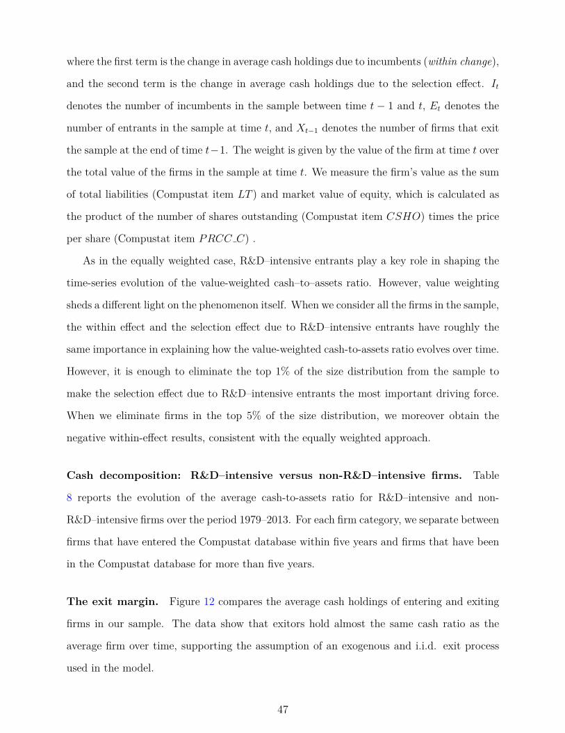
where the first term is the change in average cash holdings due to incumbents (within change),
and the second term is the change in average cash holdings due to the selection effect. It
denotes the number of incumbents in the sample between time t − 1 and t, Et denotes the
number of entrants in the sample at time t, and Xt−1 denotes the number of firms that exit
the sample at the end of time t−1. The weight is given by the value of the firm at time t over
the total value of the firms in the sample at time t. We measure the firm’s value as the sum
of total liabilities (Compustat item LT ) and market value of equity, which is calculated as
the product of the number of shares outstanding (Compustat item CSHO) times the price
per share (Compustat item PRCC C) .
As in the equally weighted case, R&D–intensive entrants play a key role in shaping the
time-series evolution of the value-weighted cash–to–assets ratio. However, value weighting
sheds a different light on the phenomenon itself. When we consider all the firms in the sample,
the within effect and the selection effect due to R&D–intensive entrants have roughly the
same importance in explaining how the value-weighted cash-to-assets ratio evolves over time.
However, it is enough to eliminate the top 1% of the size distribution from the sample to
make the selection effect due to R&D–intensive entrants the most important driving force.
When we eliminate firms in the top 5% of the size distribution, we moreover obtain the
negative within-effect results, consistent with the equally weighted approach.
Cash decomposition: R&D–intensive versus non-R&D–intensive firms. Table
8 reports the evolution of the average cash-to-assets ratio for R&D–intensive and non-
R&D–intensive firms over the period 1979–2013. For each firm category, we separate between
firms that have entered the Compustat database within five years and firms that have been
in the Compustat database for more than five years.
The exit margin. Figure 12 compares the average cash holdings of entering and exiting
firms in our sample. The data show that exitors hold almost the same cash ratio as the
average firm over time, supporting the assumption of an exogenous and i.i.d. exit process
used in the model.
47
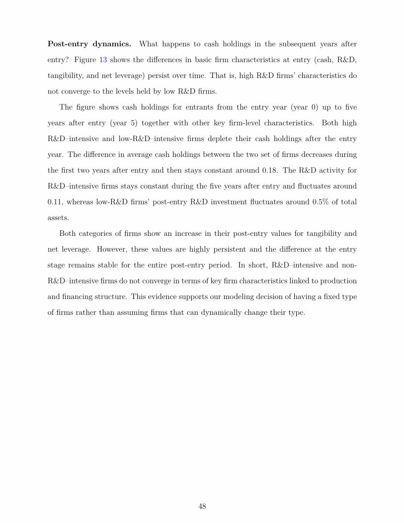
Post-entry dynamics. What happens to cash holdings in the subsequent years after
entry? Figure 13 shows the differences in basic firm characteristics at entry (cash, R&D,
tangibility, and net leverage) persist over time. That is, high R&D firms’ characteristics do
not converge to the levels held by low R&D firms.
The figure shows cash holdings for entrants from the entry year (year 0) up to five
years after entry (year 5) together with other key firm-level characteristics. Both high
R&D–intensive and low-R&D–intensive firms deplete their cash holdings after the entry
year. The difference in average cash holdings between the two set of firms decreases during
the first two years after entry and then stays constant around 0.18. The R&D activity for
R&D–intensive firms stays constant during the five years after entry and fluctuates around
0.11, whereas low-R&D firms’ post-entry R&D investment fluctuates around 0.5% of total
assets.
Both categories of firms show an increase in their post-entry values for tangibility and
net leverage. However, these values are highly persistent and the difference at the entry
stage remains stable for the entire post-entry period. In short, R&D–intensive and non-
R&D–intensive firms do not converge in terms of key firm characteristics linked to production
and financing structure. This evidence supports our modeling decision of having a fixed type
of firms rather than assuming firms that can dynamically change their type.
48
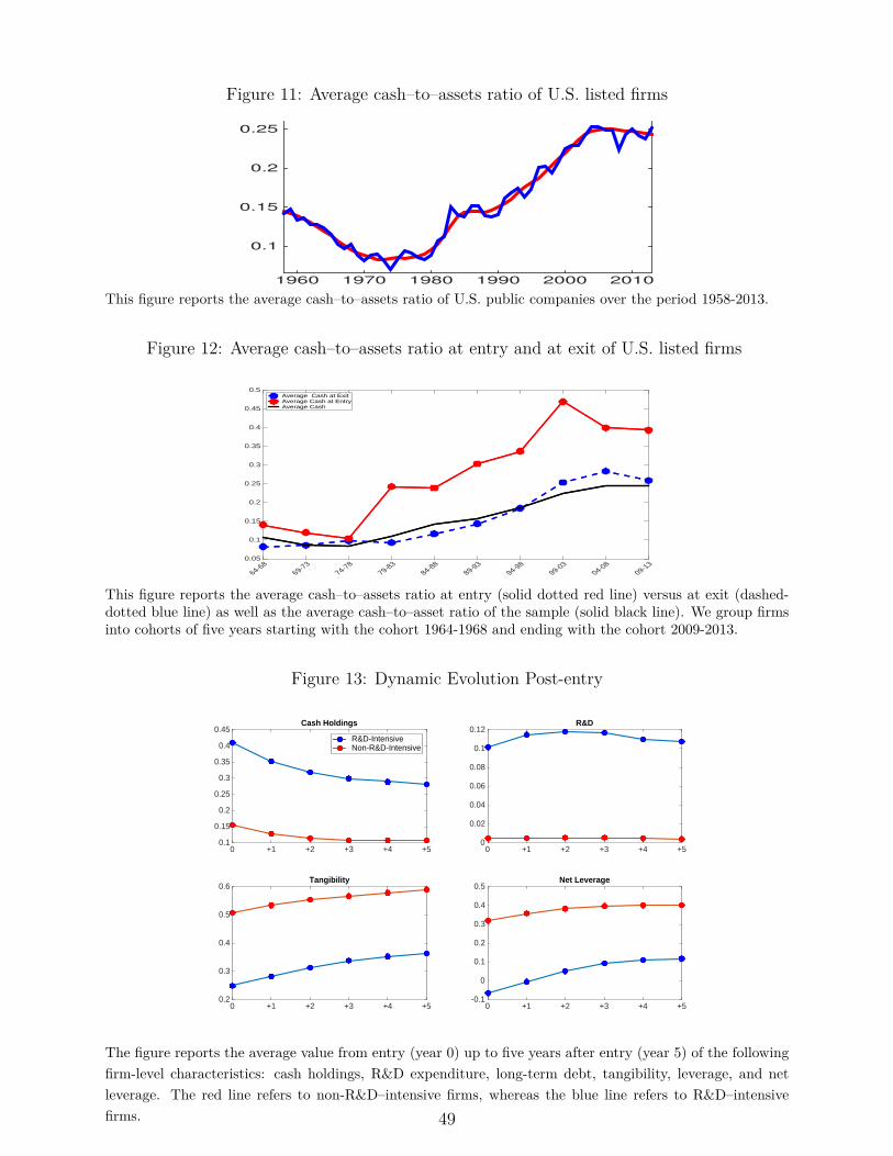
Figure 11: Average cash–to–assets ratio of U.S. listed firms
1960 1970 1980 1990 2000 2010
0.1
0.15
0.2
0.25
This figure reports the average cash–to–assets ratio of U.S. public companies over the period 1958-2013.
Figure 12: Average cash–to–assets ratio at entry and at exit of U.S. listed firms
64-6869-73
74-7879-83
84-8889-93
94-9899-03
04-0809-13
0.05
0.1
0.15
0.2
0.25
0.3
0.35
0.4
0.45
0.5 Average Cash at Exit Average Cash at Entry Average Cash
This figure reports the average cash–to–assets ratio at entry (solid dotted red line) versus at exit (dashed-dotted blue line) as well as the average cash–to–asset ratio of the sample (solid black line). We group firmsinto cohorts of five years starting with the cohort 1964-1968 and ending with the cohort 2009-2013.
Figure 13: Dynamic Evolution Post-entry
0 +1 +2 +3 +4 +50.1
0.15
0.2
0.25
0.3
0.35
0.4
0.45Cash Holdings
R&D-Intensive Non-R&D-Intensive
0 +1 +2 +3 +4 +50
0.02
0.04
0.06
0.08
0.1
0.12R&D
0 +1 +2 +3 +4 +50.2
0.3
0.4
0.5
0.6Tangibility
0 +1 +2 +3 +4 +5-0.1
0
0.1
0.2
0.3
0.4
0.5Net Leverage
The figure reports the average value from entry (year 0) up to five years after entry (year 5) of the followingfirm-level characteristics: cash holdings, R&D expenditure, long-term debt, tangibility, leverage, and netleverage. The red line refers to non-R&D–intensive firms, whereas the blue line refers to R&D–intensivefirms. 49
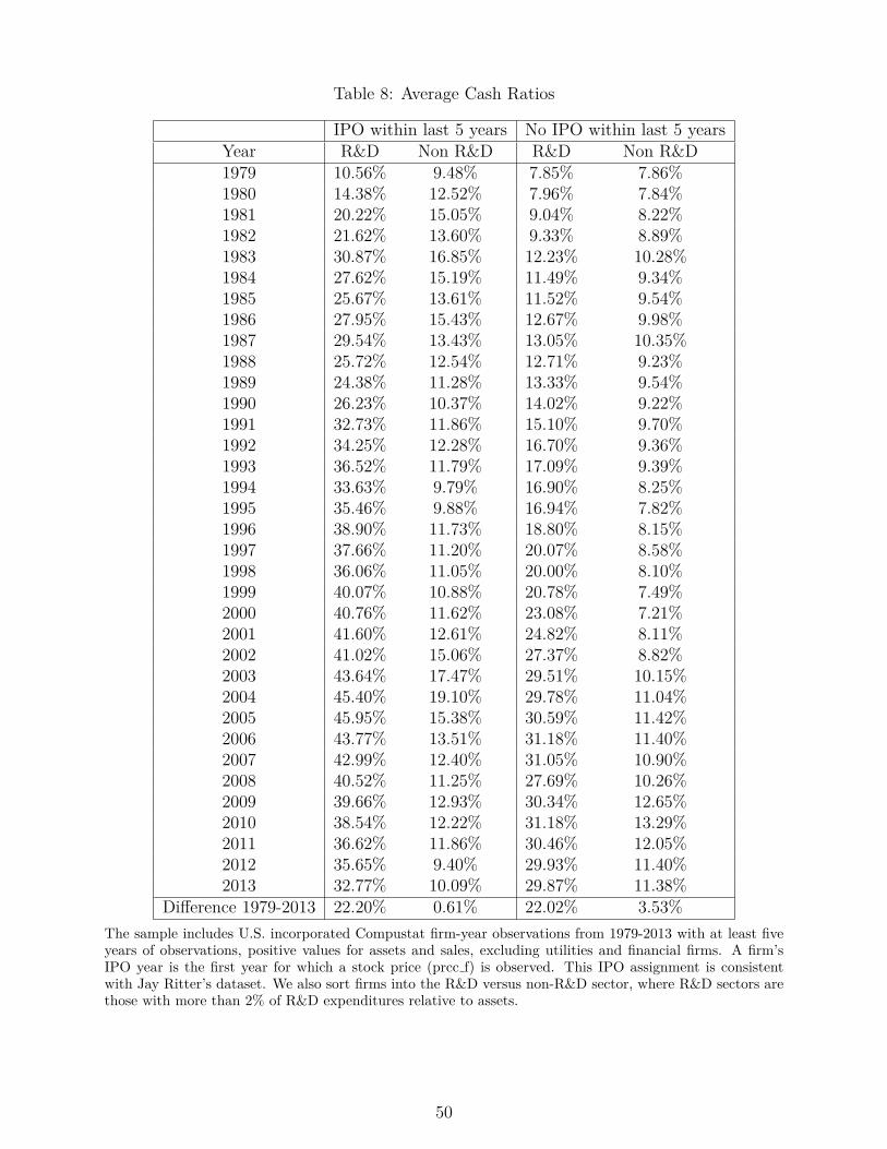
Table 8: Average Cash Ratios
IPO within last 5 years No IPO within last 5 yearsYear R&D Non R&D R&D Non R&D1979 10.56% 9.48% 7.85% 7.86%1980 14.38% 12.52% 7.96% 7.84%1981 20.22% 15.05% 9.04% 8.22%1982 21.62% 13.60% 9.33% 8.89%1983 30.87% 16.85% 12.23% 10.28%1984 27.62% 15.19% 11.49% 9.34%1985 25.67% 13.61% 11.52% 9.54%1986 27.95% 15.43% 12.67% 9.98%1987 29.54% 13.43% 13.05% 10.35%1988 25.72% 12.54% 12.71% 9.23%1989 24.38% 11.28% 13.33% 9.54%1990 26.23% 10.37% 14.02% 9.22%1991 32.73% 11.86% 15.10% 9.70%1992 34.25% 12.28% 16.70% 9.36%1993 36.52% 11.79% 17.09% 9.39%1994 33.63% 9.79% 16.90% 8.25%1995 35.46% 9.88% 16.94% 7.82%1996 38.90% 11.73% 18.80% 8.15%1997 37.66% 11.20% 20.07% 8.58%1998 36.06% 11.05% 20.00% 8.10%1999 40.07% 10.88% 20.78% 7.49%2000 40.76% 11.62% 23.08% 7.21%2001 41.60% 12.61% 24.82% 8.11%2002 41.02% 15.06% 27.37% 8.82%2003 43.64% 17.47% 29.51% 10.15%2004 45.40% 19.10% 29.78% 11.04%2005 45.95% 15.38% 30.59% 11.42%2006 43.77% 13.51% 31.18% 11.40%2007 42.99% 12.40% 31.05% 10.90%2008 40.52% 11.25% 27.69% 10.26%2009 39.66% 12.93% 30.34% 12.65%2010 38.54% 12.22% 31.18% 13.29%2011 36.62% 11.86% 30.46% 12.05%2012 35.65% 9.40% 29.93% 11.40%2013 32.77% 10.09% 29.87% 11.38%
Difference 1979-2013 22.20% 0.61% 22.02% 3.53%The sample includes U.S. incorporated Compustat firm-year observations from 1979-2013 with at least fiveyears of observations, positive values for assets and sales, excluding utilities and financial firms. A firm’sIPO year is the first year for which a stock price (prcc f) is observed. This IPO assignment is consistentwith Jay Ritter’s dataset. We also sort firms into the R&D versus non-R&D sector, where R&D sectors arethose with more than 2% of R&D expenditures relative to assets.
50
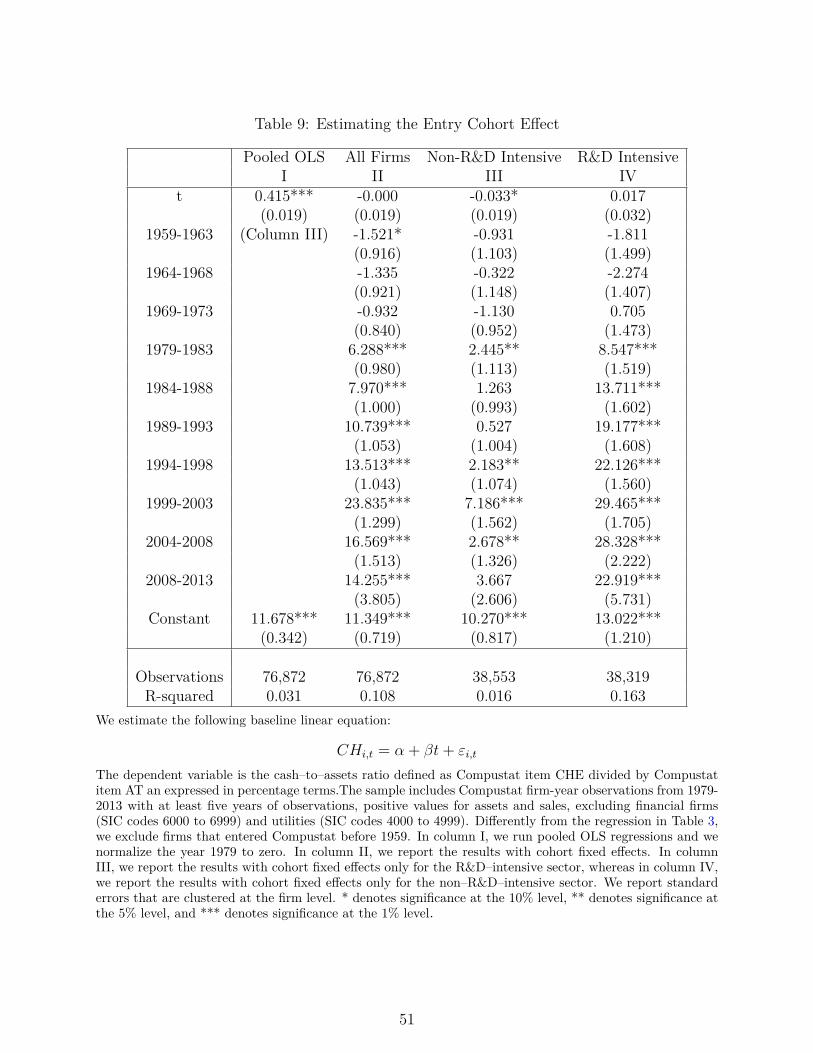
Table 9: Estimating the Entry Cohort Effect
Pooled OLS All Firms Non-R&D Intensive R&D IntensiveI II III IV
t 0.415*** -0.000 -0.033* 0.017(0.019) (0.019) (0.019) (0.032)
1959-1963 (Column III) -1.521* -0.931 -1.811(0.916) (1.103) (1.499)
1964-1968 -1.335 -0.322 -2.274(0.921) (1.148) (1.407)
1969-1973 -0.932 -1.130 0.705(0.840) (0.952) (1.473)
1979-1983 6.288*** 2.445** 8.547***(0.980) (1.113) (1.519)
1984-1988 7.970*** 1.263 13.711***(1.000) (0.993) (1.602)
1989-1993 10.739*** 0.527 19.177***(1.053) (1.004) (1.608)
1994-1998 13.513*** 2.183** 22.126***(1.043) (1.074) (1.560)
1999-2003 23.835*** 7.186*** 29.465***(1.299) (1.562) (1.705)
2004-2008 16.569*** 2.678** 28.328***(1.513) (1.326) (2.222)
2008-2013 14.255*** 3.667 22.919***(3.805) (2.606) (5.731)
Constant 11.678*** 11.349*** 10.270*** 13.022***(0.342) (0.719) (0.817) (1.210)
Observations 76,872 76,872 38,553 38,319R-squared 0.031 0.108 0.016 0.163
We estimate the following baseline linear equation:
CHi,t = α + βt+ εi,t
The dependent variable is the cash–to–assets ratio defined as Compustat item CHE divided by Compustatitem AT an expressed in percentage terms.The sample includes Compustat firm-year observations from 1979-2013 with at least five years of observations, positive values for assets and sales, excluding financial firms(SIC codes 6000 to 6999) and utilities (SIC codes 4000 to 4999). Differently from the regression in Table 3,we exclude firms that entered Compustat before 1959. In column I, we run pooled OLS regressions and wenormalize the year 1979 to zero. In column II, we report the results with cohort fixed effects. In columnIII, we report the results with cohort fixed effects only for the R&D–intensive sector, whereas in column IV,we report the results with cohort fixed effects only for the non–R&D–intensive sector. We report standarderrors that are clustered at the firm level. * denotes significance at the 10% level, ** denotes significance atthe 5% level, and *** denotes significance at the 1% level.
51
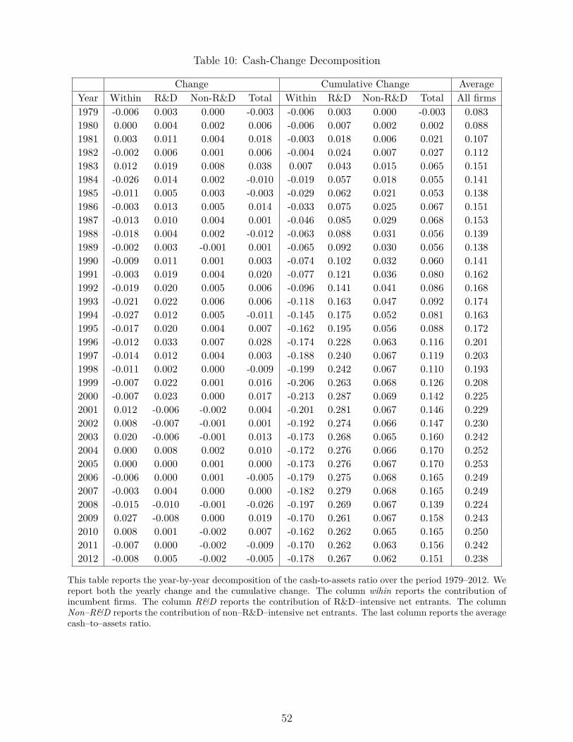
Table 10: Cash-Change Decomposition
Change Cumulative Change AverageYear Within R&D Non-R&D Total Within R&D Non-R&D Total All firms1979 -0.006 0.003 0.000 -0.003 -0.006 0.003 0.000 -0.003 0.0831980 0.000 0.004 0.002 0.006 -0.006 0.007 0.002 0.002 0.0881981 0.003 0.011 0.004 0.018 -0.003 0.018 0.006 0.021 0.1071982 -0.002 0.006 0.001 0.006 -0.004 0.024 0.007 0.027 0.1121983 0.012 0.019 0.008 0.038 0.007 0.043 0.015 0.065 0.1511984 -0.026 0.014 0.002 -0.010 -0.019 0.057 0.018 0.055 0.1411985 -0.011 0.005 0.003 -0.003 -0.029 0.062 0.021 0.053 0.1381986 -0.003 0.013 0.005 0.014 -0.033 0.075 0.025 0.067 0.1511987 -0.013 0.010 0.004 0.001 -0.046 0.085 0.029 0.068 0.1531988 -0.018 0.004 0.002 -0.012 -0.063 0.088 0.031 0.056 0.1391989 -0.002 0.003 -0.001 0.001 -0.065 0.092 0.030 0.056 0.1381990 -0.009 0.011 0.001 0.003 -0.074 0.102 0.032 0.060 0.1411991 -0.003 0.019 0.004 0.020 -0.077 0.121 0.036 0.080 0.1621992 -0.019 0.020 0.005 0.006 -0.096 0.141 0.041 0.086 0.1681993 -0.021 0.022 0.006 0.006 -0.118 0.163 0.047 0.092 0.1741994 -0.027 0.012 0.005 -0.011 -0.145 0.175 0.052 0.081 0.1631995 -0.017 0.020 0.004 0.007 -0.162 0.195 0.056 0.088 0.1721996 -0.012 0.033 0.007 0.028 -0.174 0.228 0.063 0.116 0.2011997 -0.014 0.012 0.004 0.003 -0.188 0.240 0.067 0.119 0.2031998 -0.011 0.002 0.000 -0.009 -0.199 0.242 0.067 0.110 0.1931999 -0.007 0.022 0.001 0.016 -0.206 0.263 0.068 0.126 0.2082000 -0.007 0.023 0.000 0.017 -0.213 0.287 0.069 0.142 0.2252001 0.012 -0.006 -0.002 0.004 -0.201 0.281 0.067 0.146 0.2292002 0.008 -0.007 -0.001 0.001 -0.192 0.274 0.066 0.147 0.2302003 0.020 -0.006 -0.001 0.013 -0.173 0.268 0.065 0.160 0.2422004 0.000 0.008 0.002 0.010 -0.172 0.276 0.066 0.170 0.2522005 0.000 0.000 0.001 0.000 -0.173 0.276 0.067 0.170 0.2532006 -0.006 0.000 0.001 -0.005 -0.179 0.275 0.068 0.165 0.2492007 -0.003 0.004 0.000 0.000 -0.182 0.279 0.068 0.165 0.2492008 -0.015 -0.010 -0.001 -0.026 -0.197 0.269 0.067 0.139 0.2242009 0.027 -0.008 0.000 0.019 -0.170 0.261 0.067 0.158 0.2432010 0.008 0.001 -0.002 0.007 -0.162 0.262 0.065 0.165 0.2502011 -0.007 0.000 -0.002 -0.009 -0.170 0.262 0.063 0.156 0.2422012 -0.008 0.005 -0.002 -0.005 -0.178 0.267 0.062 0.151 0.238
This table reports the year-by-year decomposition of the cash-to-assets ratio over the period 1979–2012. Wereport both the yearly change and the cumulative change. The column wihin reports the contribution ofincumbent firms. The column R&D reports the contribution of R&D–intensive net entrants. The columnNon–R&D reports the contribution of non–R&D–intensive net entrants. The last column reports the averagecash–to–assets ratio.
52
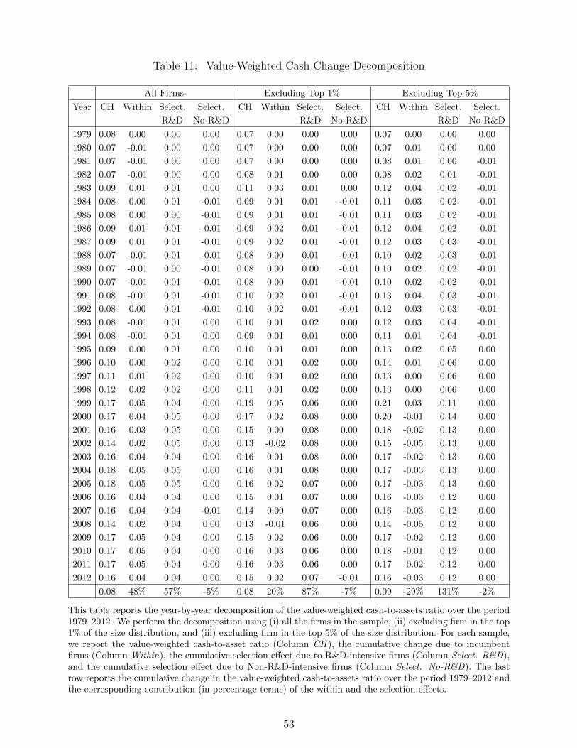
Table 11: Value-Weighted Cash Change Decomposition
All Firms Excluding Top 1% Excluding Top 5%Year CH Within Select. Select. CH Within Select. Select. CH Within Select. Select.
R&D No-R&D R&D No-R&D R&D No-R&D1979 0.08 0.00 0.00 0.00 0.07 0.00 0.00 0.00 0.07 0.00 0.00 0.001980 0.07 -0.01 0.00 0.00 0.07 0.00 0.00 0.00 0.07 0.01 0.00 0.001981 0.07 -0.01 0.00 0.00 0.07 0.00 0.00 0.00 0.08 0.01 0.00 -0.011982 0.07 -0.01 0.00 0.00 0.08 0.01 0.00 0.00 0.08 0.02 0.01 -0.011983 0.09 0.01 0.01 0.00 0.11 0.03 0.01 0.00 0.12 0.04 0.02 -0.011984 0.08 0.00 0.01 -0.01 0.09 0.01 0.01 -0.01 0.11 0.03 0.02 -0.011985 0.08 0.00 0.00 -0.01 0.09 0.01 0.01 -0.01 0.11 0.03 0.02 -0.011986 0.09 0.01 0.01 -0.01 0.09 0.02 0.01 -0.01 0.12 0.04 0.02 -0.011987 0.09 0.01 0.01 -0.01 0.09 0.02 0.01 -0.01 0.12 0.03 0.03 -0.011988 0.07 -0.01 0.01 -0.01 0.08 0.00 0.01 -0.01 0.10 0.02 0.03 -0.011989 0.07 -0.01 0.00 -0.01 0.08 0.00 0.00 -0.01 0.10 0.02 0.02 -0.011990 0.07 -0.01 0.01 -0.01 0.08 0.00 0.01 -0.01 0.10 0.02 0.02 -0.011991 0.08 -0.01 0.01 -0.01 0.10 0.02 0.01 -0.01 0.13 0.04 0.03 -0.011992 0.08 0.00 0.01 -0.01 0.10 0.02 0.01 -0.01 0.12 0.03 0.03 -0.011993 0.08 -0.01 0.01 0.00 0.10 0.01 0.02 0.00 0.12 0.03 0.04 -0.011994 0.08 -0.01 0.01 0.00 0.09 0.01 0.01 0.00 0.11 0.01 0.04 -0.011995 0.09 0.00 0.01 0.00 0.10 0.01 0.01 0.00 0.13 0.02 0.05 0.001996 0.10 0.00 0.02 0.00 0.10 0.01 0.02 0.00 0.14 0.01 0.06 0.001997 0.11 0.01 0.02 0.00 0.10 0.01 0.02 0.00 0.13 0.00 0.06 0.001998 0.12 0.02 0.02 0.00 0.11 0.01 0.02 0.00 0.13 0.00 0.06 0.001999 0.17 0.05 0.04 0.00 0.19 0.05 0.06 0.00 0.21 0.03 0.11 0.002000 0.17 0.04 0.05 0.00 0.17 0.02 0.08 0.00 0.20 -0.01 0.14 0.002001 0.16 0.03 0.05 0.00 0.15 0.00 0.08 0.00 0.18 -0.02 0.13 0.002002 0.14 0.02 0.05 0.00 0.13 -0.02 0.08 0.00 0.15 -0.05 0.13 0.002003 0.16 0.04 0.04 0.00 0.16 0.01 0.08 0.00 0.17 -0.02 0.13 0.002004 0.18 0.05 0.05 0.00 0.16 0.01 0.08 0.00 0.17 -0.03 0.13 0.002005 0.18 0.05 0.05 0.00 0.16 0.02 0.07 0.00 0.17 -0.03 0.13 0.002006 0.16 0.04 0.04 0.00 0.15 0.01 0.07 0.00 0.16 -0.03 0.12 0.002007 0.16 0.04 0.04 -0.01 0.14 0.00 0.07 0.00 0.16 -0.03 0.12 0.002008 0.14 0.02 0.04 0.00 0.13 -0.01 0.06 0.00 0.14 -0.05 0.12 0.002009 0.17 0.05 0.04 0.00 0.15 0.02 0.06 0.00 0.17 -0.02 0.12 0.002010 0.17 0.05 0.04 0.00 0.16 0.03 0.06 0.00 0.18 -0.01 0.12 0.002011 0.17 0.05 0.04 0.00 0.16 0.03 0.06 0.00 0.17 -0.02 0.12 0.002012 0.16 0.04 0.04 0.00 0.15 0.02 0.07 -0.01 0.16 -0.03 0.12 0.00
0.08 48% 57% -5% 0.08 20% 87% -7% 0.09 -29% 131% -2%
This table reports the year-by-year decomposition of the value-weighted cash-to-assets ratio over the period1979–2012. We perform the decomposition using (i) all the firms in the sample, (ii) excluding firm in the top1% of the size distribution, and (iii) excluding firm in the top 5% of the size distribution. For each sample,we report the value-weighted cash-to-asset ratio (Column CH ), the cumulative change due to incumbentfirms (Column Within), the cumulative selection effect due to R&D-intensive firms (Column Select. R&D),and the cumulative selection effect due to Non-R&D-intensive firms (Column Select. No-R&D). The lastrow reports the cumulative change in the value-weighted cash-to-assets ratio over the period 1979–2012 andthe corresponding contribution (in percentage terms) of the within and the selection effects.
53