Finite Element Modeling of anUltrasonic Transducer

S. Moten

D&C 2011.006

Literature Survey

Coach(es): dr.ir N. Mihajlovic (Philips Research)

Supervisor: prof.dr. H. Nijmeijer

Eindhoven University of TechnologyDepartment of Mechanical EngineeringDynamics & Control Group

Eindhoven, January, 2011

Abstract

Ultrasonic transducers are integrated into the minimally invasive needles andcatheters for medical diagnostic. There is a need for a model that can predict thebehavior of the ultrasonic transducer. Many designers employ one dimensionalanalytic models, however due to certain limitations these models are not adequateto understand the entire performance of an ultrasonic transducer.

Nowadays, finite element modeling is being adopted in the design of ultrasonictransducers. The purpose is to get more realistic transducer simulations and toaccelerate the design process. In this report, a literature survey is presented in or-der to model the complete ultrasonic measurement system using the finite elementmethod.

i

ii

Preface

This literature survey is written as a part of the graduation thesis in Dynamics andControl group at department of Mechanical Engineering, Eindhoven University ofTechnology (TU/e). It is pleasure for me to thank all those who made this possible.

First of all, I owe my deepest gratitude to Prof. Henk Nijmeijer (TU/e) who madehis support available in a number of ways and made it possible to work on such aninteresting topic in Philips Research (High Tech Campus).

I am heartily thankful to Dr. ir. Nenad Mihajlovic (Philips Research) whose encour-agement and guidance enabled me to develop firm understanding of the subject.Finally, I would like to thank the whole team working on transducer in MinimallyInvasive Healthcare group (Philips Research), with whom I can discuss and shareideas in a pleasant environment.

Last but not least, I want to pay regards and blessings to my parents who alwaysstood behind me for support.

Sikandar Moten, EindhovenDecember, 2010

iii

iv

Contents

Abstract i

Preface iii

Contents v

1 Introduction 1

1.1 Cardiac Ablation . . . . . . . . . . . . . . . . . . . . . . . . . . . . . . 1

1.2 Ultrasonic Measurement System–System Description . . . . . . . . . 2

1.3 Report Outlook and Organization . . . . . . . . . . . . . . . . . . . . . 3

2 Literature Survey 5

2.1 Transducer Design . . . . . . . . . . . . . . . . . . . . . . . . . . . . . 5

2.1.1 Basic configuration of the ultrasonic transducer . . . . . . . . 5

2.1.2 Quarter-wave acoustic matching . . . . . . . . . . . . . . . . . 5

2.1.3 Backing layer . . . . . . . . . . . . . . . . . . . . . . . . . . . . 7

2.1.4 Electrical matching . . . . . . . . . . . . . . . . . . . . . . . . . 8

2.2 Transducer Modeling . . . . . . . . . . . . . . . . . . . . . . . . . . . . 8

2.2.1 One-dimensional modeling . . . . . . . . . . . . . . . . . . . . 8

2.2.2 Three-dimensional modeling . . . . . . . . . . . . . . . . . . . 9

2.3 Vibration Characteristics of a Piezoelectric Disc . . . . . . . . . . . . . 10

2.4 Finite Element Modeling of the Piezoelectric Ultrasonic Transducer . 12

2.4.1 Formulation of the piezoelectric effect . . . . . . . . . . . . . . 12

2.4.2 Formulation of the acoustic waves propagation . . . . . . . . 13

v

CONTENTS

2.4.3 Finite element method . . . . . . . . . . . . . . . . . . . . . . . 15

2.4.4 The Electric Circuit . . . . . . . . . . . . . . . . . . . . . . . . . 19

2.5 Material Characterization . . . . . . . . . . . . . . . . . . . . . . . . . 20

2.5.1 Characterization of passive materials . . . . . . . . . . . . . . 21

2.5.2 Characterization of active materials . . . . . . . . . . . . . . . 23

2.6 Incremental Validation . . . . . . . . . . . . . . . . . . . . . . . . . . . 24

2.6.1 Step by step validation . . . . . . . . . . . . . . . . . . . . . . . 25

2.6.2 Impedance measurement . . . . . . . . . . . . . . . . . . . . . 26

2.7 Performance Measurement and Validation . . . . . . . . . . . . . . . 26

2.7.1 Pulse-echo testing . . . . . . . . . . . . . . . . . . . . . . . . . 27

2.7.2 Acoustic output measurement and beam plots . . . . . . . . . 27

3 Conclusion and Recommendations 29

3.1 Conclusion . . . . . . . . . . . . . . . . . . . . . . . . . . . . . . . . . . 29

3.2 Recommendations . . . . . . . . . . . . . . . . . . . . . . . . . . . . . 30

References 33

vi

Chapter 1

Introduction

In this chapter, we discuss an application for which we need to model the ultra-sonic transducer in an ultrasonic measurement system. This provides motivationto develop a basic understanding for the ultrasonic measurement system.

1.1 Cardiac Ablation

The heart is a pump that functions by pumping the blood in a controlled sequencethrough its four chambers: left atrium, right atrium, left ventricle and right ventri-cle. Each heart beat originates as an electrical impulse from a small area of tissuein the right atrium of the heart called the sinus node. The impulse initially causesboth of the atria to contract, then activates the atrioventricular node which is nor-mally the only electrical connection between the atria and the ventricles. The im-pulse then spreads through both ventricles causing a synchronized contraction ofthe heart muscle.

For a healthy person, this regular flow of electricity through defined paths is thebasis of normal heart muscle contractions which results in normal heart beat. How-ever, sometimes this flow of electricity becomes irregular due to a faulty electricalpathway and, consequently, the heart beats very erratically. Such heart diseasesare termed arrhythmia in medical science. In adults the normal resting heart rateranges from 60 to 80 beats per minute. The resting heart rate in children is muchfaster.

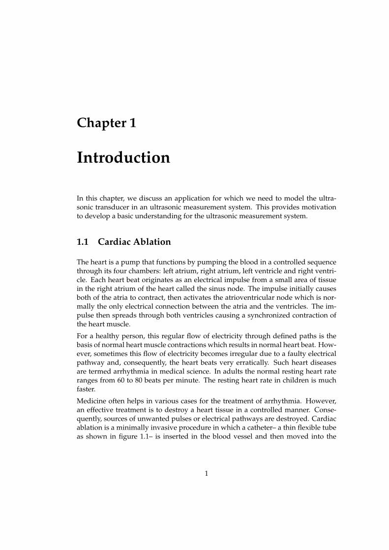
Medicine often helps in various cases for the treatment of arrhythmia. However,an effective treatment is to destroy a heart tissue in a controlled manner. Conse-quently, sources of unwanted pulses or electrical pathways are destroyed. Cardiacablation is a minimally invasive procedure in which a catheter– a thin flexible tubeas shown in figure 1.1– is inserted in the blood vessel and then moved into the

1

Introduction

heart by surgeons. Once the tip of the catheter has reached the targeted place intothe heart, Radio Frequency(RF) energy is used to destroy the tissue.

Figure 1.1: A typical catheter used for ablation [Courtesy: Philips Research]

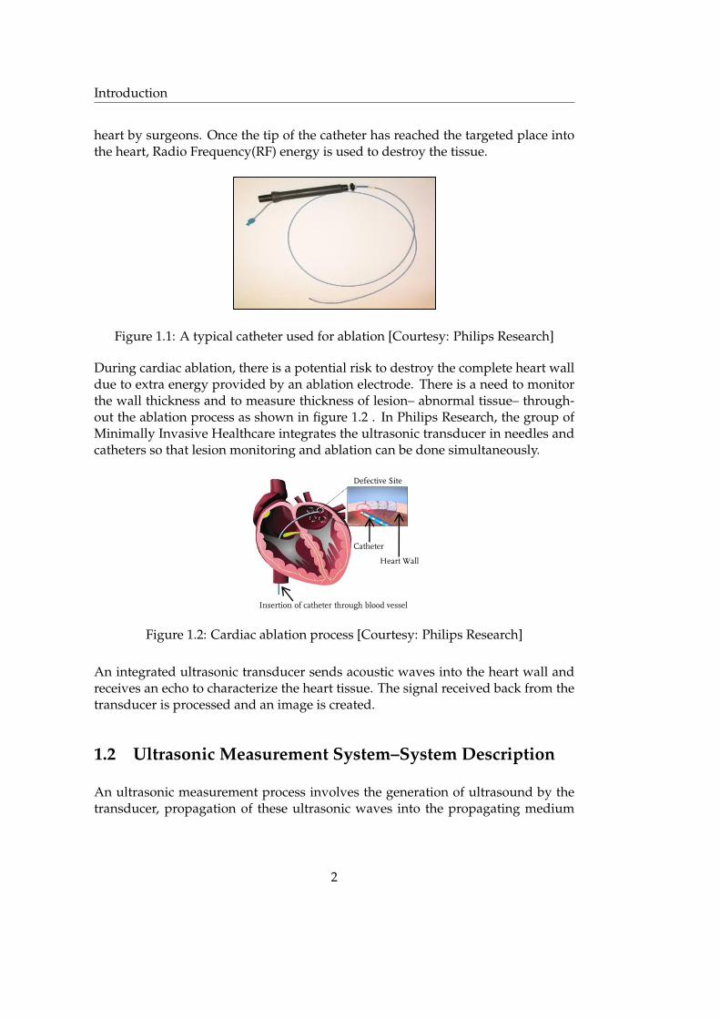
During cardiac ablation, there is a potential risk to destroy the complete heart walldue to extra energy provided by an ablation electrode. There is a need to monitorthe wall thickness and to measure thickness of lesion– abnormal tissue– through-out the ablation process as shown in figure 1.2 . In Philips Research, the group ofMinimally Invasive Healthcare integrates the ultrasonic transducer in needles andcatheters so that lesion monitoring and ablation can be done simultaneously.

Catheter

Heart Wall

Insertion of catheter through blood vessel

Defective Site

Figure 1.2: Cardiac ablation process [Courtesy: Philips Research]

An integrated ultrasonic transducer sends acoustic waves into the heart wall andreceives an echo to characterize the heart tissue. The signal received back from thetransducer is processed and an image is created.

1.2 Ultrasonic Measurement System–System Description

An ultrasonic measurement process involves the generation of ultrasound by thetransducer, propagation of these ultrasonic waves into the propagating medium

2

Introduction

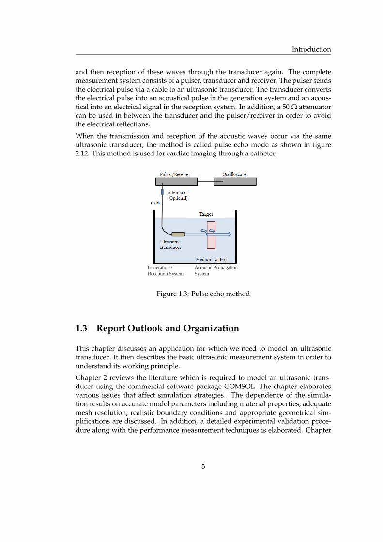
and then reception of these waves through the transducer again. The completemeasurement system consists of a pulser, transducer and receiver. The pulser sendsthe electrical pulse via a cable to an ultrasonic transducer. The transducer convertsthe electrical pulse into an acoustical pulse in the generation system and an acous-tical into an electrical signal in the reception system. In addition, a 50 Ω attenuatorcan be used in between the transducer and the pulser/receiver in order to avoidthe electrical reflections.

When the transmission and reception of the acoustic waves occur via the sameultrasonic transducer, the method is called pulse echo mode as shown in figure2.12. This method is used for cardiac imaging through a catheter.

Generation /

Reception System

Acoustic Propagation

System

Figure 1.3: Pulse echo method

1.3 Report Outlook and Organization

This chapter discusses an application for which we need to model an ultrasonictransducer. It then describes the basic ultrasonic measurement system in order tounderstand its working principle.

Chapter 2 reviews the literature which is required to model an ultrasonic trans-ducer using the commercial software package COMSOL. The chapter elaboratesvarious issues that affect simulation strategies. The dependence of the simula-tion results on accurate model parameters including material properties, adequatemesh resolution, realistic boundary conditions and appropriate geometrical sim-plifications are discussed. In addition, a detailed experimental validation proce-dure along with the performance measurement techniques is elaborated. Chapter

3

Introduction

3 summarizes the salient features of the complete discussion and gives concludingremarks.

4

Chapter 2

Literature Survey

2.1 Transducer Design

Traditionally, the design of an ultrasonic transducer is normally accomplished viaestablished "rules of thumb" and fundamental theoretical understanding. Afteran initial design is made, the performance of the transducer is analyzed eitherby a simple analytic one-dimensional model or a three-dimensional finite elementmodel. Before we start with the design guideline for a single element transducer, itis necessary to understand the basic configuration of the transducer.

2.1.1 Basic configuration of the ultrasonic transducer

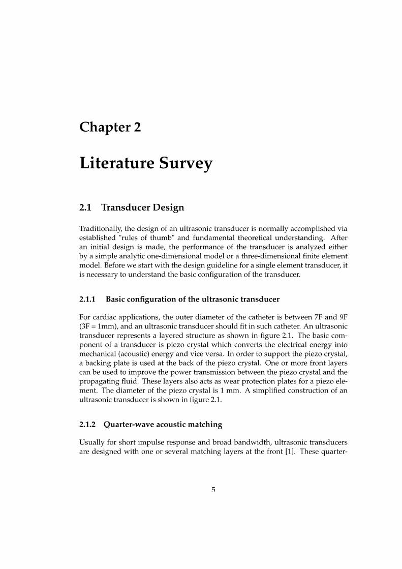
For cardiac applications, the outer diameter of the catheter is between 7F and 9F(3F = 1mm), and an ultrasonic transducer should fit in such catheter. An ultrasonictransducer represents a layered structure as shown in figure 2.1. The basic com-ponent of a transducer is piezo crystal which converts the electrical energy intomechanical (acoustic) energy and vice versa. In order to support the piezo crystal,a backing plate is used at the back of the piezo crystal. One or more front layerscan be used to improve the power transmission between the piezo crystal and thepropagating fluid. These layers also acts as wear protection plates for a piezo ele-ment. The diameter of the piezo crystal is 1 mm. A simplified construction of anultrasonic transducer is shown in figure 2.1.

2.1.2 Quarter-wave acoustic matching

Usually for short impulse response and broad bandwidth, ultrasonic transducersare designed with one or several matching layers at the front [1]. These quarter-

5

Literature Survey

Matching layer

Piezo ceramic disc

Backing layer

Catheter

Physical Design

7F(3F = 1mm)

Figure 2.1: Simplified construction of an ultrasonic transducer inside a catheter

wave front layers are used to improve the energy transmission from the piezocrystal to the acoustic medium. For designing an ultrasonic transducer for in-vivo (within the living) applications, material of the front layer should also be bio-compatible.

McKeighen in [1] mentions that the transmission line theory can be used to choosethe front layers such that these layers provide matching between impedance of thepiezo ceramic Zpiezo and impedance of the acoustic medium Zmed. According totransmission line theory, the optimal acoustic impedances for one or two matchinglayer are:For one layer:

Zlayer =√

ZpiezoZmed (2.1)

For two layers:

Zlayer1 = Zpiezo3/4Zmed

1/4

Zlayer2 = Zpiezo1/4Zmed

3/4(2.2)

For the design of a wide-band transducer, Desilets et al. in [2] modify the choice offront layers using the KLM theory. They consider the first half of a piezoceramicas a quarter-wave matching layer, in addition to the quarter wave matching layersattached to the ceramic. Their analysis dictates the choice of the matching layersas:For one layer:

Zlayer = Zpiezo1/3Zmed

2/3 (2.3)

6

Literature Survey

For two layers:

Zlayer1 = Zpiezo4/7Zmed

3/7

Zlayer2 = Zpiezo1/7Zmed

6/7 (2.4)

The addition of more than one matching layer increases the complexity to manu-facture the transducer. However, this also increases the efficiency of the transducerand results in the improvement of both the bandwidth and sensitivity.

2.1.3 Backing layer

To select an appropriate backing layer, there are several design considerationswhich need to be considered. Brown in [3] discusses in detail about these designconsiderations. Based on that discussion, the following design considerations arenecessary to take into account.

1. The impedance of the backing material has to be according to the requiredbandwidth of the ultrasonic transducer. For the cardiac application, we needhigh bandwidth transducers. This gives a fast ringing down of the signal and,a higher resolution for imaging. However, increasing the bandwidth with anincrease of the backing impedance, also decreases the efficiency [4] and thusthe signal to noise ratio (SNR). This means there is a tradeoff between theseparameters.

2. The attenuation coefficient of the backing material should be as high as possi-ble so that acoustic waves transmitted to the back cannot reflect back and wereceive an echo without interference.

There are other design considerations which do not influence the performance ofthe ultrasonic transducer but these are necessary for manufacturing the transducer.

1. The backing material should be easy to machine and should be shaped intodifferent thickness and size.

2. The backing material should have good adhesion properties so that it canadhere with the piezoelectric material.

3. The backing material should have high surface quality to ease the transfer ofenergy to the back and to reduce noise.

7

Literature Survey

2.1.4 Electrical matching

The electrical impedance of an ultrasonic transducer depends on the material prop-erties of the active element (piezo ceramic) as well as the effects of the front match-ing layers and the backing layer [5]. There is a high chance that the impedance ofa designed transducer does not match with the impedance of the connected cableand transceiver (pulser/receiver) at the transducer resonant frequency. This elec-trical impedance mismatch creates the electrical reflections between the transducerand cable and between the cable and transceiver. In order to avoid these electri-cal reflections, which can cause artifacts in the image, the following solutions aresuggested in [5].

1. The basic electrical elements (preferably capacitors and inductors) can beplaced in series or shunt (as per the design requirement) between the cableand transducer and/or between the cable and transceiver to match the elec-trical impedances.

2. A coaxial cable itself can be used to match the impedance of the trans-ducer with the transceiver. In this approach, the electrical impedance of thetransceiver Zelec and the electrical impedance of the transducer Ztran at thetransducer resonant frequency dictate the choice of the electrical impedanceof the cable as given below.

Zcable =√

ZelecZtran (2.5)

In order to transfer the maximum power, the length of the cable should beequal to the quarter wavelength of the signal within the cable.

Any of the above "rules" not only removes the electrical reflections but also in-creases the energy transmission, which consequently improves the signal to noiseratio and bandwidth of the received echo signal.

2.2 Transducer Modeling

2.2.1 One-dimensional modeling

Two well known one-dimensional analytic models are Mason’s and the KLMmodel, see [6]. These models are equivalent circuit models for a piezo crystal anduse different electrical configuration, see [7]. The transducer has a backing layer atthe back and single (or multiple) layer(s) at the front side. In order to model thecomplete transducer, we also need a model of the backing layer and the front layer

8

Literature Survey

separately. For the detailed modeling process and implementation using the Ma-son’s model, see [8]. Both Mason’s and KLM model are one-dimensional in natureand are very effective in predicting the response of an ultrasonic transducer. Thesemodels are computationally very cheap and help to accelerate the product designcycles. Besides many advantages, these models have the following limitations aswell:

• The model is one-dimensional, therefore only a one-dimensional pressurefield can be investigated.

• The model assumed that the thickness of the backing layer is semi-infinitewithout losses [9]. This means that any acoustic wave transmitted to the backdoes not reflect back from other interfaces. In reality, these reflections caninterfere with the received echo from the front side, if the backing layer hasless attenuation.

• The model is made for a piezo crystal having the lateral dimensions muchlarger than the thickness. In practice, due to severe space limitations, thepiezo crystal does not satisfy these geometrical constraints. Consequently,the model results will become unreliable and less accurate.

• The model is made for a thin, loss-less, disc shaped piezo crystal. It is notvalid for a lossy piezo ceramic and polymer based piezo element. For thisreason, several authors (such as [10] and [11]) modified the actual electricalconfiguration of the standard circuit to introduce losses inside a piezo crystal.

• The model is made to simulate an ultrasonic transducer. It cannot simulatethe interactions of other objects with the transducer (such as catheter capshown in figure 2.1).

2.2.2 Three-dimensional modeling

A finite element model for an ultrasonic transducer provides a realistic transducersimulation and gives a way to visualize the real acoustic wave propagation into theacoustic medium [12]. Using the finite element method, we can cope with all thelimitations described above for one-dimensional model, such as:

• Using the finite element model a three-dimensional pressure field can be in-vestigated.

• Finite element models are based on the governing equations of the acousticpropagation and piezoelectricity, so back reflections from any interface can bemodeled and investigated.

9

Literature Survey

• With the 3D or 2D axisymmetric models, we can simulate all the vibrationmodes upon the excitation of a piezo crystal layer. There is no geometricalconstraint for accurate simulations.

• The losses in the materials (both in active and passive materials) can be mod-eled easily by setting the appropriate material properties.

• The interaction of the acoustic field of an ultrasonic transducer with otherobjects can be simulated.

Besides the above advantages, finite element modeling has certain disadvantagesas well. In order to obtain required accuracy at high frequencies, the finite elementmodel of an ultrasonic transducer comprises of several thousands to few milliondegrees of freedom. Such a large model requires computer systems with extensiveprocessing capabilities and considerable effort to build, debug and operate.

Another disadvantage of finite element modeling is that the response of a trans-ducer can differ substantially from the actual response. This can be due to theuse of an inadequate number of elements to resolve acoustic waves, unrealisticboundary conditions or less accurate model parameters (such as material proper-ties). These disadvantages indicate the need for experimental validation of a finiteelement model. This will be discussed in a latter section.

2.3 Vibration Characteristics of a Piezoelectric Disc

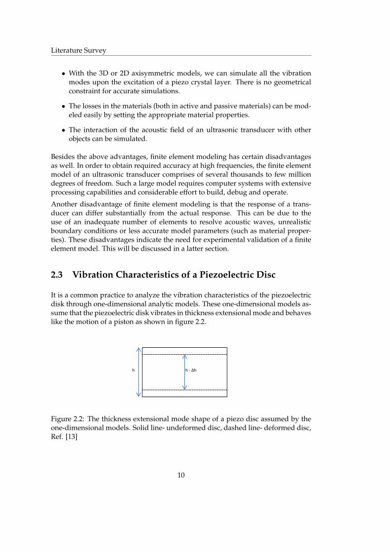
It is a common practice to analyze the vibration characteristics of the piezoelectricdisk through one-dimensional analytic models. These one-dimensional models as-sume that the piezoelectric disk vibrates in thickness extensional mode and behaveslike the motion of a piston as shown in figure 2.2.

h - Δhh

Figure 2.2: The thickness extensional mode shape of a piezo disc assumed by theone-dimensional models. Solid line- undeformed disc, dashed line- deformed disc,Ref. [13]

10

Literature Survey

Guo et al. mention in [13] that these one-dimensional methods are applicable toa piezo disk with diameter to thickness (d/h) ratios greater than or around 20.This is due to the fact that under such geometrical constraint, the vibration char-acteristic related to the thickness extensional mode becomes dominant. However,many designers employ the disc with the d/h ratios much less than 20 due to spacelimitations in their design. In these cases, the use of the finite element method toanalyze the vibration characteristics of a piezoelectric disc becomes indispensable.

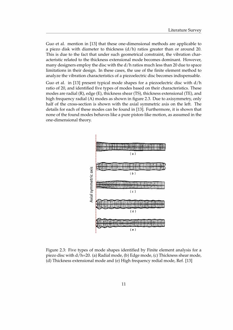
Guo et al. in [13] present typical mode shapes for a piezoelectric disc with d/hratio of 20, and identified five types of modes based on their characteristics. Thesemodes are radial (R), edge (E), thickness shear (TS), thickness extensional (TE), andhigh frequency radial (A) modes as shown in figure 2.3. Due to axisymmetry, onlyhalf of the cross-section is shown with the axial symmetric axis on the left. Thedetails for each of these modes can be found in [13]. Furthermore, it is shown thatnone of the found modes behaves like a pure piston-like motion, as assumed in theone-dimensional theory.

Axi

al s

ymm

etri

c ax

is

Figure 2.3: Five types of mode shapes identified by Finite element analysis for apiezo disc with d/h=20. (a) Radial mode, (b) Edge mode, (c) Thickness shear mode,(d) Thickness extensional mode and (e) High frequency redial mode, Ref. [13]

11

Literature Survey

It implies that the one-dimensional models are no longer adequate to completelyanalyze the performance of an ultrasonic transducer. It is therefore necessary toanalyze the piezoelectric transducer using a complete three dimensional model.The finite element method (FEM) has a great flexibility to analyze the piezo elementdisc independently and with the layered structured inside an ultrasonic transducer.

2.4 Finite Element Modeling of the Piezoelectric UltrasonicTransducer

An ultrasonic measurement process involves the generation of ultrasound by thetransducer and propagation of the acoustic waves into the propagating medium. Itis important to see the formulation of the governing equations for the piezoelectricdevice and wave propagation in the acoustic medium.

2.4.1 Formulation of the piezoelectric effect

2.4.1.1 The piezoelectric effect

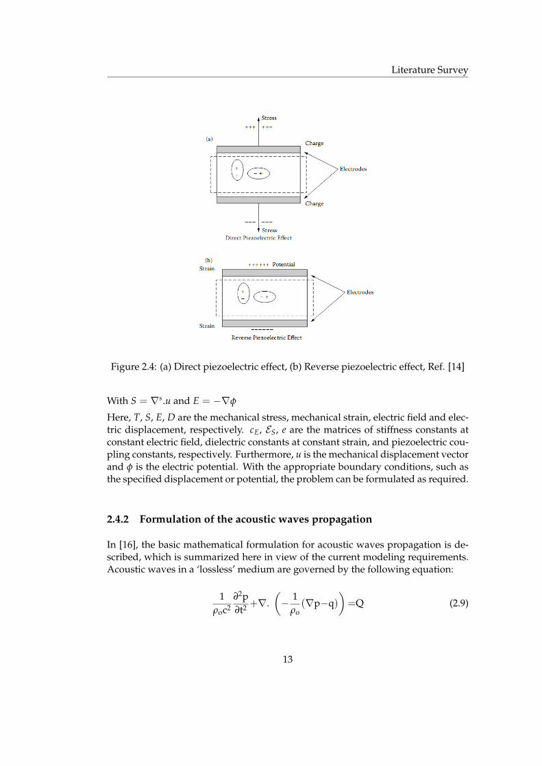
The piezoelectric effect involves the conversion of electric energy to mechanical en-ergy and vice versa. The direct and reverse piezoelectric effects are shown in figure2.4. The direct effect consists of the generation of net charge across the electrodesupon the application of stress, whereas the reverse piezoelectric effect refers to thephenomenon in which an applied electric potential across the electrodes induces adeformation of the crystal.

2.4.1.2 The piezoelectric constitutive relations

Abboud et al. in [15] express the governing equations of the linear piezoelectricityalong with the equations of the mechanical and electric balance as:

Constitutive equations:

T = cE.S− eT.ED = e.S + ES.E (2.6)

Momentum balance:ρu = ∇.T (2.7)

Electric balance:∇.D = 0 (2.8)

12

Literature Survey

Figure 2.4: (a) Direct piezoelectric effect, (b) Reverse piezoelectric effect, Ref. [14]

With S = ∇s.u and E = −∇φ

Here, T, S, E, D are the mechanical stress, mechanical strain, electric field and elec-tric displacement, respectively. cE, ES, e are the matrices of stiffness constants atconstant electric field, dielectric constants at constant strain, and piezoelectric cou-pling constants, respectively. Furthermore, u is the mechanical displacement vectorand φ is the electric potential. With the appropriate boundary conditions, such asthe specified displacement or potential, the problem can be formulated as required.

2.4.2 Formulation of the acoustic waves propagation

In [16], the basic mathematical formulation for acoustic waves propagation is de-scribed, which is summarized here in view of the current modeling requirements.Acoustic waves in a ‘lossless’ medium are governed by the following equation:

1ρoc2

∂2p∂t2 +∇.

(− 1

ρo(∇p−q)

)=Q (2.9)

13

Literature Survey

Here, p is the acoustic pressure in the medium, ρo is the density of the acousticmedium, c is the speed of sound in the medium, q and Q are the monopole anddipole sources respectively.

The acoustic medium with lossy behavior can be modeled by using a complexspeed of sound and a complex density. Various fluid models are available in theCOMSOL (a commercial FEM package) such as linear elastic, linear elastic with at-tenuation, Delany-Bazley (for a porous medium), viscous medium and ideal gasmodels. Each of these models has its own formulation, details can be found in [16].When there is a need to model the transient behavior, only certain frequency depen-dencies can be modeled, which limits the number of fluid models. In time domainan additional term of first order time derivative can account for attenuation of thesound waves, as shown below:

1ρoc2

∂2p∂t2 −da

∂p∂t

+∇.(− 1

ρo(∇p−q)

)=Q (2.10)

Here, da is the damping coefficient

The quality and accuracy of the results is dependent on the accurate boundaryconditions. Below are typical boundary conditions which can be used during anmodeling exercise,

• Sound hard boundary - Zero acceleration condition

• Sound soft boundary - Zero acoustic pressure condition

• Acceleration boundary condition - Specified normal acceleration at theboundary

• Pressure boundary condition - Specified acoustic pressure at the boundary

• Continuity boundary condition - Equal acceleration at the interface betweenparts in an assembly

• Impedance boundary condition - Specified impedance condition at the theboundary

• Non reflecting boundary condition - To allow an outgoing wave to leave themedium with minimum reflections

• Axial symmetry boundary condition - For axisymmetric geometries to reducethe dimensions

14

Literature Survey

2.4.3 Finite element method

We have seen that governing equations for both the piezoelectric effect and acousticwave propagation involve partial differential equations. The finite element methodis one of the possible numerical techniques that can be used to find the approximatesolutions for partial differential equations. Nowadays, thanks to the commerciallyavailable packages (such as COMSOL, ANSYS, ABAQUS, PZFLEX etc.) for solvingcomplex problems by the finite element method. However, a modeler or designerneeds to know various aspects involve in the finite element modeling to accuratelymodel and analyze a problem. Many authors including [15], [17], [12], [18] etc.adopted finite element method to analyze the ultrasonic transducer.

Modeling of an ultrasonic measurement system using a finite element approachinvolves various issues. This includes a careful selection of the mesh resolutionto resolve waves, artificial boundary conditions and model connections to the realworld (surroundings), damping of the the real world materials etc. In what follows,we discuss some of the fundamental modeling issues underlying the finite elementsimulation of the ultrasonic transducer propagating in the acoustic medium.

2.4.3.1 Spatial discretization

The resolution of a solution provided by the finite element model is defined by itsmesh. The solutions of the wave propagation problems are wave like in nature.These waves are characterized by the wavelength λ in space. The dependence ofwavelength on the frequency f and speed of sound c in a acoustic medium is givenby:

λ = c/ f (2.11)

For wave propagation problems, the spatial discretization must be defined suchthat it can resolve the shortest wavelength (i.e. highest frequency) of interest [15].To have a meaningful solution on the discrete grid, at least two degrees of freedomper wavelength is required [16]. However, such a coarse solution is useless to ana-lyze. In practice, the designer needs adequate resolution of the solution. In [16], itis recommended to use 12 degrees of freedom per wavelength to get an adequatesolution rather than a borderline solution. As in most cases, the direction of prop-agation is not known before analysis, so it is better to use the isotropic mesh. Thisgives the following rules of thumb to calculate the number of degrees of freedom(DOFs).

• For 1D, Number of DOFs = 12 times the length of a model geometry measuredin wavelengths

15

Literature Survey

• For 2D, Number of DOFs = 144 times the area of a model geometry measuredin wavelengths squared

• For 3D, Number of DOFs = 1728 times the volume of a model geometry mea-sured in wavelengths cubed

Nowadays, a 32-bit computer system can usually deal somewhere from a few hun-dred thousand up to a million degrees of freedom [16], using the commercial soft-ware package COMSOL. It is a good practice to estimate the number of degrees offreedom in a model before hand, as it can help the modeler to take certain decisionsregarding the model simplifications.

2.4.3.2 Analyzing model convergence

Convergence of a finite element model is necessary to obtain an accurate solution.Although the rules of thumb indicated above (i.e. use 12 DOFs per wavelength)is adequate, it is recommended in [16] to perform a convergence test to check ifthe mesh density is sufficient. In such a test, a modeler refines the mesh, runsthe study again, and then checks if the solution converges to a stable value. Ifthe solution changes after the mesh refinement then it means that the solution ismesh dependent. Such a unstable solution dictates the need of a finer mesh. Thisconvergence test should be performed until the solution converges to a stable value.The commercial FEM package COMSOL offers adaptive mesh refinement, whichadds mesh elements based on an error criterion to resolve those areas where theerror is large.

2.4.3.3 Axial symmetry

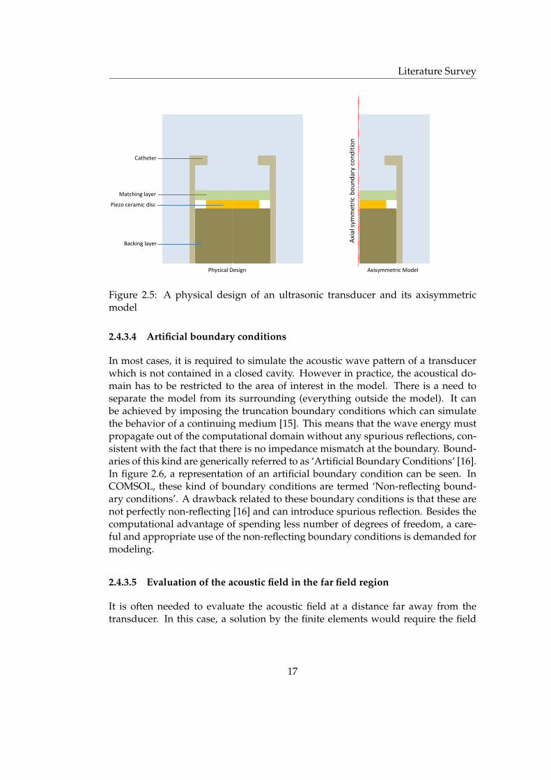
When the geometry of the ultrasonic transducer has cylindrical shape, it is imprac-tical to model the full 3D model of the transduction device and surrounding acous-tic media for the axial symmetric geometries. Usually, the transducer in a catheterhas a circular piezo ceramic disc. So, we can take advantage of the axial symmetryand model the transducer in a 2D domain. In figure 2.5, a 2D axisymmetric modelof a transducer enclosed in a catheter is shown. By using a 2D axisymmetric ge-ometry instead of the complete 3D geometry, we can reduce the number of degreesof freedom dramatically and save a lot of computational resources. Many authorsincluding [12] have taken advantage of axisymmetric geometry of the transducerand modeled the transducer with a 2D axisymmetric geometry. Furthermore, Guoet al. in [13] found the vibration characteristics of a piezo disc through a 2D axisym-metric geometry.

16

Literature Survey

Matching layer

Piezo ceramic disc

Backing layer

Catheter

Physical Design Axisymmetric Model

Axi

al s

ymm

etri

c b

ou

nd

ary

con

dit

ion

Figure 2.5: A physical design of an ultrasonic transducer and its axisymmetricmodel

2.4.3.4 Artificial boundary conditions

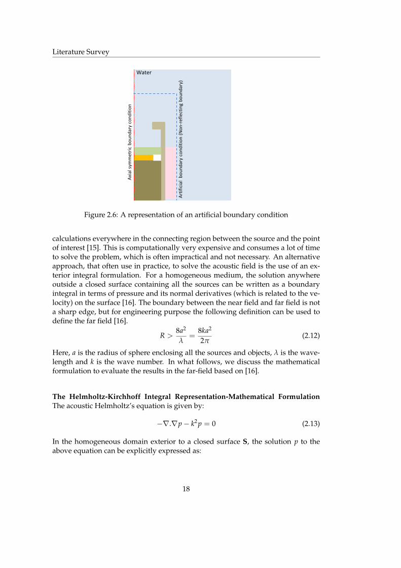
In most cases, it is required to simulate the acoustic wave pattern of a transducerwhich is not contained in a closed cavity. However in practice, the acoustical do-main has to be restricted to the area of interest in the model. There is a need toseparate the model from its surrounding (everything outside the model). It canbe achieved by imposing the truncation boundary conditions which can simulatethe behavior of a continuing medium [15]. This means that the wave energy mustpropagate out of the computational domain without any spurious reflections, con-sistent with the fact that there is no impedance mismatch at the boundary. Bound-aries of this kind are generically referred to as ‘Artificial Boundary Conditions’ [16].In figure 2.6, a representation of an artificial boundary condition can be seen. InCOMSOL, these kind of boundary conditions are termed ‘Non-reflecting bound-ary conditions’. A drawback related to these boundary conditions is that these arenot perfectly non-reflecting [16] and can introduce spurious reflection. Besides thecomputational advantage of spending less number of degrees of freedom, a care-ful and appropriate use of the non-reflecting boundary conditions is demanded formodeling.

2.4.3.5 Evaluation of the acoustic field in the far field region

It is often needed to evaluate the acoustic field at a distance far away from thetransducer. In this case, a solution by the finite elements would require the field

17

Literature Survey

Axisymmetric Model

Axi

al s

ymm

etri

c b

ou

nd

ary

con

dit

ion

Art

ific

ial

bo

un

dar

y co

nd

itio

n (

No

n-r

efle

ctin

g b

ou

nd

ary)

Water

Figure 2.6: A representation of an artificial boundary condition

calculations everywhere in the connecting region between the source and the pointof interest [15]. This is computationally very expensive and consumes a lot of timeto solve the problem, which is often impractical and not necessary. An alternativeapproach, that often use in practice, to solve the acoustic field is the use of an ex-terior integral formulation. For a homogeneous medium, the solution anywhereoutside a closed surface containing all the sources can be written as a boundaryintegral in terms of pressure and its normal derivatives (which is related to the ve-locity) on the surface [16]. The boundary between the near field and far field is nota sharp edge, but for engineering purpose the following definition can be used todefine the far field [16].

R >8a2

λ=

8ka2

2π(2.12)

Here, a is the radius of sphere enclosing all the sources and objects, λ is the wave-length and k is the wave number. In what follows, we discuss the mathematicalformulation to evaluate the results in the far-field based on [16].

The Helmholtz-Kirchhoff Integral Representation-Mathematical FormulationThe acoustic Helmholtz’s equation is given by:

−∇.∇p− k2 p = 0 (2.13)

In the homogeneous domain exterior to a closed surface S, the solution p to theabove equation can be explicitly expressed as:

18

Literature Survey

p (R) =∫

S(G (R, r) ∇p (r)−∇G (R, r) p (r) ) .ndS (2.14)

Here, the unit vector n is directed into the domain enclosed by S, which means npoints normal outwards to the exterior infinite domain. The close surface S is pa-rameterized by the coordinate vector r. The function G (R, r) is the Green’s functionsatisfying the following equation:

−∇.∇G (R, r)− k2G (R, r) = δ(3)(R− r) (2.15)

The Green’s function itself is a function of the vector r of an outgoing wave excitedby a source at R. For the 3D case, this Green’s function can be written as:

G (R, r) =e−ik|r−R|

4π |r−R| (2.16)

Substituting the above Green’s function into the general solution for the pressure(equation (2.14)), we have the following expression for the solution:

p (R) =1

4π

∫S

e−ik|r−R|

|r−R|

(∇p (r) + p (r)

1 + ik |r−R||r−R|2

(r−R)

).ndS (2.17)

For the 2D axial symmetric geometry, evaluation of the 3D integral is necessarywhich needs 3D geometry. To accommodate this problem, COMSOL uses an adap-tive numerical quadrature in the azimuthal direction on a fictitious revolved geom-etry, in addition to the standard mesh-based quadrature in the 2D rz-plane [16].

2.4.4 The Electric Circuit

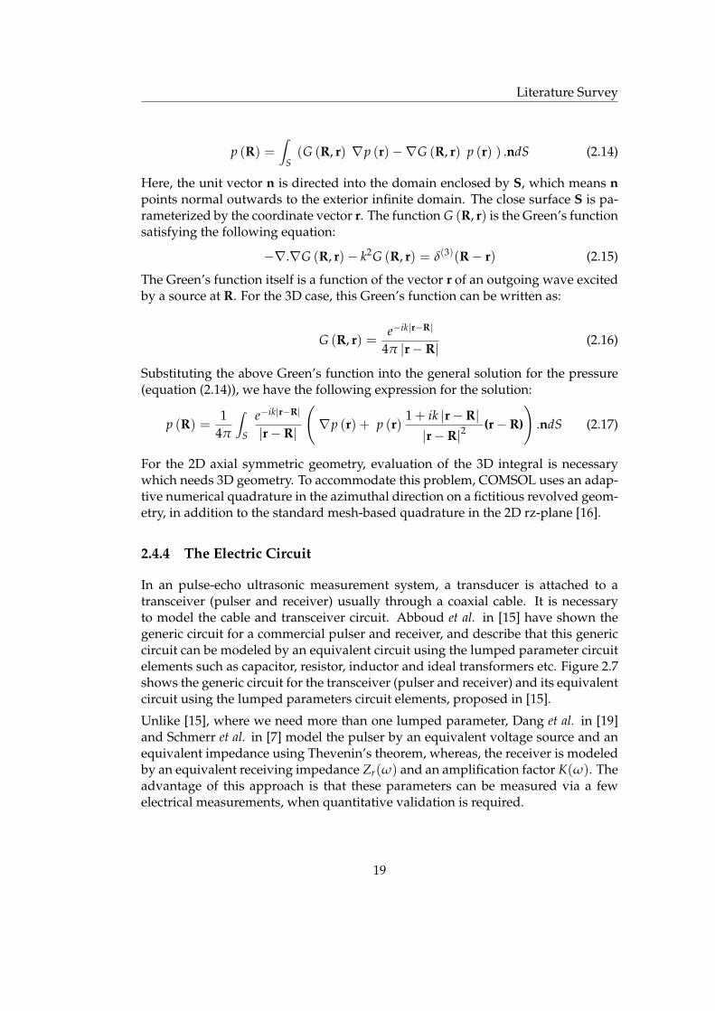
In an pulse-echo ultrasonic measurement system, a transducer is attached to atransceiver (pulser and receiver) usually through a coaxial cable. It is necessaryto model the cable and transceiver circuit. Abboud et al. in [15] have shown thegeneric circuit for a commercial pulser and receiver, and describe that this genericcircuit can be modeled by an equivalent circuit using the lumped parameter circuitelements such as capacitor, resistor, inductor and ideal transformers etc. Figure 2.7shows the generic circuit for the transceiver (pulser and receiver) and its equivalentcircuit using the lumped parameters circuit elements, proposed in [15].

Unlike [15], where we need more than one lumped parameter, Dang et al. in [19]and Schmerr et al. in [7] model the pulser by an equivalent voltage source and anequivalent impedance using Thevenin’s theorem, whereas, the receiver is modeledby an equivalent receiving impedance Zr(ω) and an amplification factor K(ω). Theadvantage of this approach is that these parameters can be measured via a fewelectrical measurements, when quantitative validation is required.

19

Literature Survey

Generic circuit for a commercial pulser Generic circuit for a commercial receiver

TRANSDUCER

TRANSDUCER

Equivalent circuit for a commercial pulser Equivalent circuit for a commercial receiver

TRANSDUCER

TRANSDUCER

Figure 2.7: Generic circuit for pulser and receiver and their equivalent representa-tion, adapted from [15]

2.5 Material Characterization

Accuracy of both the one-dimensional equivalent circuit model and three-dimensional finite element model depends on the accuracy of the material con-stitutive properties. For one dimensional piston model, we need only the longi-tudinal properties of the material. In contrast, a three dimensional finite elementmodel needs material properties both in the longitudinal and transverse directions.Established protocols are crucial to characterize the materials if we want to use amodel as a designing and a virtual prototyping tool. The properties available in themanufacturer specification sheets are often incomplete or sometimes there is a needto characterize a new material (with unknown properties) for certain requirements(e.g. making of a highly attenuating backing material). In the sequel, we discusssome established protocols available in the literature to characterize the active andpassive materials.

20

Literature Survey

2.5.1 Characterization of passive materials

The matching and backing layers in an ultrasonic transducer (see Figure 2.5) comein the category of the passive materials. For a one-dimensional model, we onlyneed the longitudinal speed of sound and the attenuation constant, but for a threedimensional model we also need shear properties. An experimental setup that canbe used to measure these properties and the method to find these properties aredescribed next.

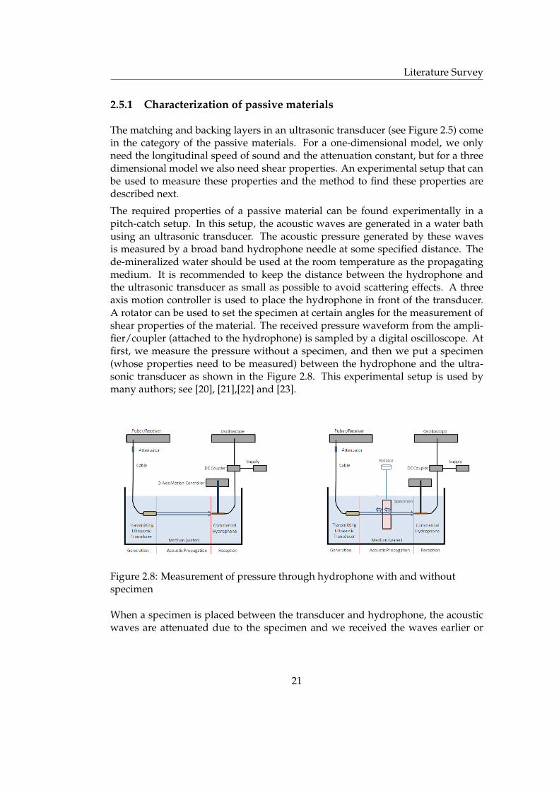
The required properties of a passive material can be found experimentally in apitch-catch setup. In this setup, the acoustic waves are generated in a water bathusing an ultrasonic transducer. The acoustic pressure generated by these wavesis measured by a broad band hydrophone needle at some specified distance. Thede-mineralized water should be used at the room temperature as the propagatingmedium. It is recommended to keep the distance between the hydrophone andthe ultrasonic transducer as small as possible to avoid scattering effects. A threeaxis motion controller is used to place the hydrophone in front of the transducer.A rotator can be used to set the specimen at certain angles for the measurement ofshear properties of the material. The received pressure waveform from the ampli-fier/coupler (attached to the hydrophone) is sampled by a digital oscilloscope. Atfirst, we measure the pressure without a specimen, and then we put a specimen(whose properties need to be measured) between the hydrophone and the ultra-sonic transducer as shown in the Figure 2.8. This experimental setup is used bymany authors; see [20], [21],[22] and [23].

Rotator

Specimen

Figure 2.8: Measurement of pressure through hydrophone with and withoutspecimen

When a specimen is placed between the transducer and hydrophone, the acousticwaves are attenuated due to the specimen and we received the waves earlier or

21

Literature Survey

later depending on the speed of sound. In order to calculate the longitudinal speedof sound in the material and the attenuation constant, several authors discuss aboutthe time domain techniques, see [20].

For the materials with high attenuation constant, the wave shape for the pressurewave changes dramatically as it transmitted through the material. In order to locatethe equivalent points for finding the amplitude ratio is detrimental [21], using timedomain signals. Other authors use frequency domain techniques developed bySachse and Pao (1978), see [23]. Wang et al. in [23] explicitly mention the formulaeto calculate the longitudinal speed of sound and attenuation constant, as givenbelow:

cl =cw

1 +(ϕ− ϕw + 2π f4t)cw

2π f d

(2.18)

αl = αw +1d

20log10

(Tl Aw

A

)(2.19)

In equations (2.18) and (2.19),4t is the trigger delay of the signal, cw is the speed ofsound in water, f is the frequency, d is the thickness of the specimen, Aw, A, ϕw andϕ are the amplitude and phase spectra, obtained by taking the Fourier transforma-tion of the time domain pressure signal, without and with a specimen respectively.Tl is the product of the transmission coefficients for the interface of water to speci-men and specimen to water:

Tl = Tw−→sTs−→w =4zwzl

(zw + zl)2 (2.20)

Here, zw and zl are the specific acoustic impedances of the water and specimenrespectively. When the acoustic wave is incident at an angle on the object otherthan 0, a shear wave is generated by the mode conversion effect [23]. Wang et al.in [23] mention the formulae to calculate the shear speed of sound and attenuationconstant, as given below:

cs =cw√

sin2(θi) +

[(ϕs − ϕw + 2π f4t)cw

2π f d+ cos(θi)

]2(2.21)

αs = αw cos(θ − θi) +1d

20log10

(Ts Aw

As

)(2.22)

In equations (2.21) and (2.22), θi is the incident angle, θ is the refractive angle ofshear waves and can be calculated from the Snell’s law. Ts is the product of the

22

Literature Survey

transmission coefficients for the interface of water to specimen and specimen towater:

Ts = Tw−→sTs−→w =4zwzs

(zw + zs)2 (2.23)

Here, zw and zs are the specific acoustic impedances of the water and specimen (inshear position) respectively. In this way, we can characterize the passive materialsfor the model.

2.5.2 Characterization of active materials

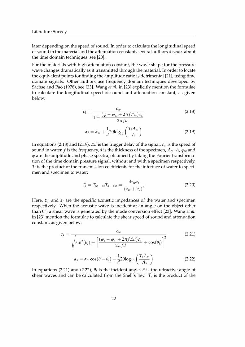
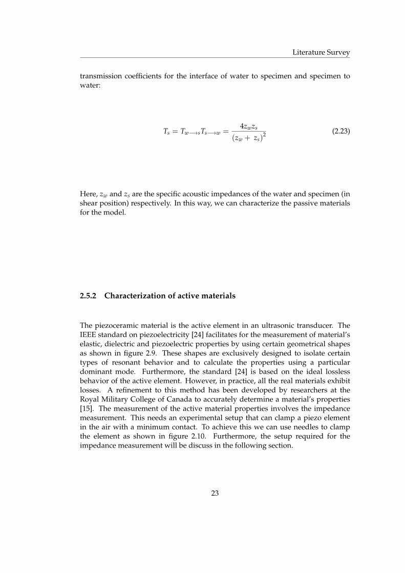
The piezoceramic material is the active element in an ultrasonic transducer. TheIEEE standard on piezoelectricity [24] facilitates for the measurement of material’selastic, dielectric and piezoelectric properties by using certain geometrical shapesas shown in figure 2.9. These shapes are exclusively designed to isolate certaintypes of resonant behavior and to calculate the properties using a particulardominant mode. Furthermore, the standard [24] is based on the ideal losslessbehavior of the active element. However, in practice, all the real materials exhibitlosses. A refinement to this method has been developed by researchers at theRoyal Military College of Canada to accurately determine a material’s properties[15]. The measurement of the active material properties involves the impedancemeasurement. This needs an experimental setup that can clamp a piezo elementin the air with a minimum contact. To achieve this we can use needles to clampthe element as shown in figure 2.10. Furthermore, the setup required for theimpedance measurement will be discuss in the following section.

23

Literature Survey

Figure 2.9: Exclusively designed geometries for different modes, adapted from [18],[15] based on IEEE standard [24]

102 micron

1 mm

Needles

Piezo disc

Schematic Real View

Piezo disc

Figure 2.10: Schematic and actual experimental setup for the measurement of piezoelement

2.6 Incremental Validation

In order to make use of the full scale model of an ultrasonic transducer propagat-ing in an acoustic medium, the quantitative validation of the model with the experi-

24

Literature Survey

mental results is crucial. Powell et al. in [18] describes an incremental "model-build-test" validation exercise to precisely model the complete ultrasonic transducer. Thestep by step procedure reported in the paper allows the user to tune the modelat different step of manufacturing before the complete simulation of the measure-ment system. Abboud et al. in [15] discusses about the same technique to validatethe model step by step.

During the manufacturing of the transducer, the piezoceramic element undergoeselevated temperatures and other complex manufacturing steps. This may causepartial depoling of the piezoceramic disc inside the transducer. Due to this fact,Powell et al. in [18] found 5% depoling of the piezo element and 10% reducedvalue of the speed of sound in the second matching layer with respect to the nom-inal material properties. Therefore, by correlating the experimental result with thesimulation one can tune the material properties, which might be off from the nom-inal properties due to the measurement errors during material characterization orthe complex manufacturing process.

The work presented in [18] is performed to validate the individual components ofan array configuration of the transducers. This is completely applicable for a singletransducer as well.

2.6.1 Step by step validation

A summary of the methodology adopted in [18] can be written in terms of differentsteps as given below.

1. Model the piezo ceramic element in air using the finite element method, basedon the properties of the piezo ceramic material

2. Correlate the impedance curve of the model and real piezo element

3. Tune the material properties of the active element, if needed

4. Add a passive layer to the model, as per the order of the manufacturing pro-cess

5. Correlate the input impedance curve of the model and the newly manufac-tured configuration

6. Tune the material properties of the newly added passive layer, if needed

7. Goto step 3 until all the passive layers will be added to the model

8. Assume the depoling effect in order to correlate the impedance curve of thecomplete configuration

25

Literature Survey

9. Now, correlate the input impedance of the complete transducer both in water

10. Put the transducer in the required package e.g in a catheter

11. Simulate the complete transducer in the required acoustic medium to analyzethe output acoustic field

12. Modify the transducer geometry (if needed) and and go to step 11

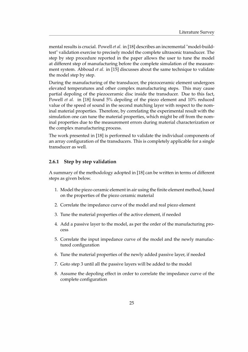
2.6.2 Impedance measurement

Both for the material characterization and incremental validation process we needto measure the input impedance. A network analyzer of appropriate frequencyrange can be used for this purpose. Before measuring the impedance, it is necessaryto calibrate the network analyzer for the open, short and known load (50 Ω usuallyused) termination conditions. Once the calibration is done, the input impedanceof a transducer or piezo element can be measured in any acoustic medium. Figure2.11 shows the measurement setup in this regard.

Network Analyzer

Loads for calibration Transducer propagating in an acoustic medium

Figure 2.11: Measurement setup for the impedance measurement

2.7 Performance Measurement and Validation

Electrical measurements (such as the transducer impedance measurements) pro-vide only an indirect measure of the acoustic performance [25]. To check the perfor-mance of a transduction device propagating in an acoustic medium, the followingstandard measurements and validation procedures can be adopted depending onthe need of a designer.

26

Literature Survey

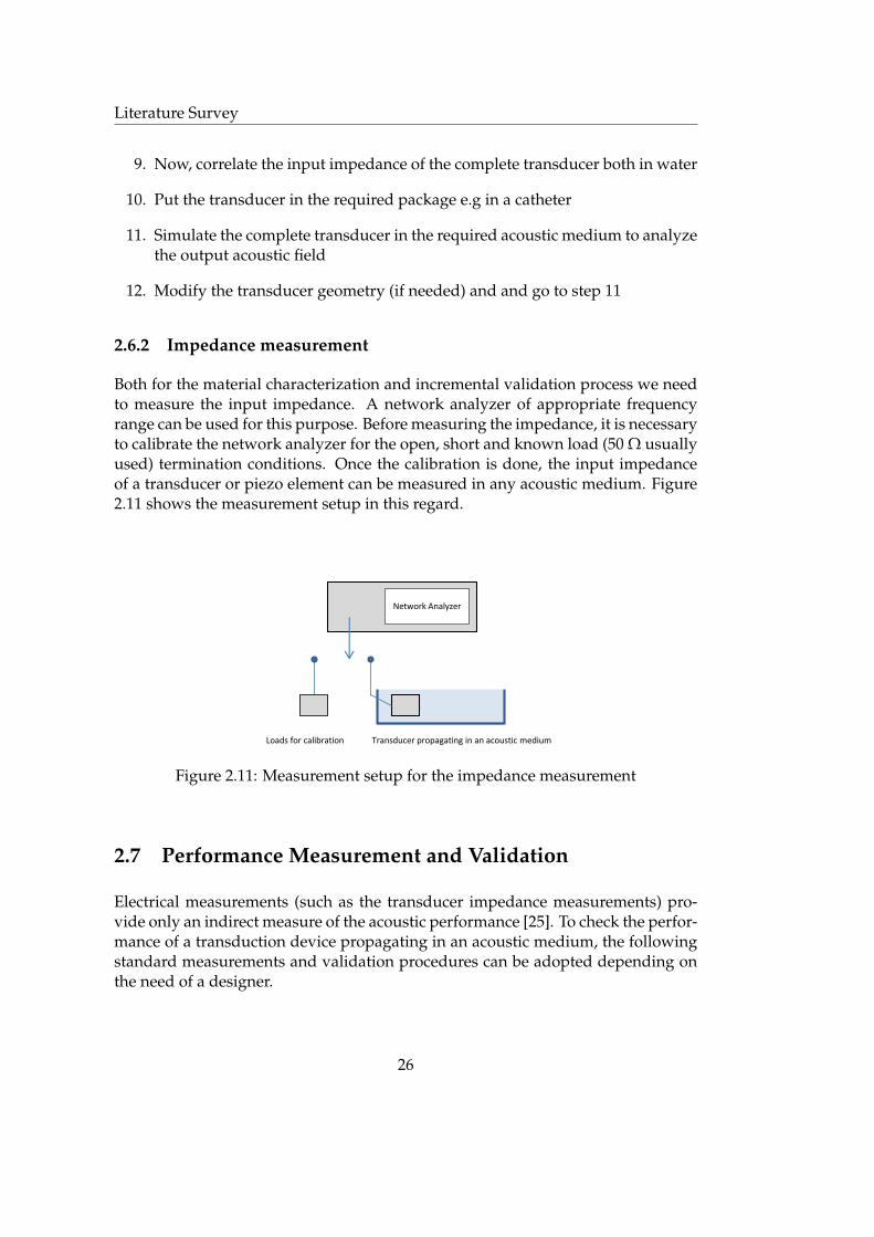
2.7.1 Pulse-echo testing

One of the standard measures of the transducer acoustic performance is a pulse-echo test [25]. In this method, a transducer is excited (usually by an impulse) andthe round-trip signal from an aligned target is obtained as shown in figure 2.12. Thereceived signal is transformed into the frequency domain by a Fast Fourier trans-formation. This transformed signal is used to find the transducer bandwidth (atvarious levels e.g.-6dB) and the sensitivity. This testing is very common in practice,because the transducer is used in a pulse-echo mode for the imaging applications.

Generation /

Reception System

Acoustic Propagation

System

Figure 2.12: Pulse echo method

2.7.2 Acoustic output measurement and beam plots

Hydrophones are a type of transducer used to measure pressure waves over anextremely wide bandwidth at an infinitesimally small spatial point [25]. A similarsetup shown in figure 2.8 is used for measuring the acoustic pressure by the hy-drophone. Medina et al. in [12] measure the acoustic pressure by a hydrophone atcertain distances to validate their 2D axisymmetric transducer model.

A further extension of this measurement can be made by setting the transducer ata fixed position and align the hydrophone along the acoustic axis by translatingin x, y, and z direction and rotation along the vertical axis. After alignment, thehydrophone is translated with a predefined resolution either in a horizontal planeor in a vertical plane to measure the acoustic pressure at different spatial points.Then a particular feature of the acoustic waveform, such as peak-to-peak voltageor signal amplitude, is determined and plotted. This kind of plot is referred asbeam plot. It is common to normalize the beam plot to the largest value measured

27

Literature Survey

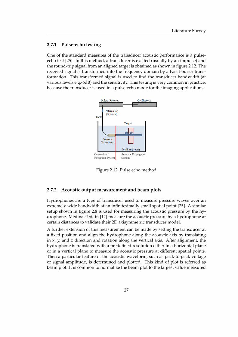
(for qualitative analysis) and present the data as a contour map with the contoursrepresenting decibel levels. Gutierrez et al. in [17] compared the normalized beamplot obtained by the simulation and experiment for the qualitative analysis of atransducer, as shown in figure 2.13

Figure 2.13: Normalized beam plot, measured for the model validation in [17]

28

Chapter 3

Conclusion and Recommendations

3.1 Conclusion

The field of medical diagnostic using ultrasonic transducers is moving forward ata rapid pace. Many designers employ one dimensional analytic models to predictthe behavior of the ultrasonic transducer. However, due to certain limitations thesemodels are not adequate to understand the entire performance of an ultrasonictransducer. Nowadays, finite element modeling is being adopted in the design ofultrasonic transducers. The objective is to get more realistic transducer simulationsand to accelerate the design process.

The purpose of this literature study is to serve as a primer for modeling an ul-trasonic transducer using the commercial software package COMSOL. The reportelaborates various issues that arise during the finite element modeling of an ul-trasonic transducer. The present study starts with basic transducer configurationand design guidelines. The breadth of this report focuses on the background andpractical modeling issues that affect simulation strategies. The dependence of thesimulation results on accurate model parameters including material properties, ad-equate mesh resolution, realistic boundary conditions and appropriate geometricalsimplifications are discussed. Various standard procedures to characterize mate-rial properties for both active and passive materials are presented. As modelingis the part of transducer design, so it is not independent of the experimental val-idation. In addition, a detailed experimental validation procedure along with theperformance measurement techniques is elaborated.

29

Conclusion and Recommendations

3.2 Recommendations

The study presented in this report highlights various aspects of finite elementacoustic modeling. Although these issues are not all-encompassing, it provides abasic foundation to a modeler or a designer for modeling an ultrasonic transducerusing finite element methods.

The modeling process involved in this report is not only useful for the ultrasonictransducer used in cardiac application, but, it is applicable to any ultrasonic mea-surement system for diagnostic and inspection. Such a system can be a non-destructive evaluation system for an aerospace structure or underwater pipe lineinspection or any medical diagnostic system. New horizons need to be found forthe application of ultrasonic transducers either by using a single ultrasonic trans-ducer or in array. In future, the need of ultrasonic transducers in medical diagnos-tics can be more demanding due to the reduction in size of ultrasonic transducersto micro scale level.

30

References

[1] R. E. McKeighen, “Design guidelines for medical ultrasonic arrays,” SPIE In-ternational Symposium on Medical Imaging, vol. 3341(2), pp. 2–18, 1998.

[2] C. S. Desilets, J. D. Fraser, and G. S. Kino, “The design of efficient broad-bandpiezoelectric transducers,” Sonics and Ultrasonics, IEEE transactions, vol. 25(3),pp. 115–125, 1978.

[3] L.F. Brown, “The effects of material selection for backing and wearprotection/quarter-wave matching of piezoelectric polymer ultrasound trans-ducers,” IEEE Ultrasonic Symposium, vol. 2, pp. 1029–1032, 2000.

[4] S.J.H. van Kervel and J.M. Thijssen, “A calculation scheme for he optimumdesign of ultrasonic transducers,” Ultrasonics, vol. 21(3), pp. 134–140, 1983.

[5] J. M. Cannata, T. A. Ritter, W. H. Chen, R. H. Silverman, and K. K. Shung, “De-sign of efficient, broadband single element (20-80 mhz) ultrasonic transducersfor medical imaging applications,” Ultrasonics, Ferroelectrics and frequency Con-trol, IEEE transactions, vol. 56(11), pp. 1548–1557, 2003.

[6] C. Dang, L.W. Schmerr Jr., and A. Sedov, “Modeling and measurement all theelements of an ultrasonic nondestructive evaluation system I: Modeling foun-dations,” Research in Nondestructive Evaluation, vol. 14(4), pp. 141–176, 2002.

[7] L.W. Schmerr and S.J. Song, Ultrasonic nondestructive evaluation system: Modeland Measurements. Springer, 2007.

[8] S. Moten, “Modeling of an ultrasonic transducer for cardiac imaging,” Tech.Rep. D&C 2010.049, Dynamics and Control Group, Eindhoven University ofTechnology, 2010.

[9] J.Assaad, M. Ravez, C. Bruneel, J.M. Rouvaen, and F. Haine, “Influence of thethickness and attenuation coeficeint of a backing on the response of transduc-ers,” Ultrasonics, vol. 34, pp. 103–106, 1996.

31

[10] A. Putterman, P. Hauptmann, Ralf Lucklum, Olaf Krause, and B. Henning,“SPICE model for lossy piezoceramic transducers,” Ultrasonics, Ferroelectricsand frequency Control, IEEE transactions, vol. 44(1), pp. 60–66, 1997.

[11] L. F. Brown and D. L. Carlson, “Ultrasound transducer models for piezoelec-tric polymer films,” Ultrasonics, Ferroelectrics and frequency Control, IEEE trans-actions, vol. 36(3), pp. 313–318, 1989.

[12] J.E.S.M. Medina, F. Buiochi, and J.C. Adamowski, “Numerical modeling of acircular piezoelectric ultrasonic transducer radiating in water,” ABCM Sympo-sium Series in Mechatronics, vol. 2, pp. 458–464, 2006.

[13] N.Guo, P. Cawley, and D. Hitchings, “The finite element analysis of the vi-bration characteristics of piezoelectric disc,” Journal of Sound and Vibration,vol. 159(2), pp. 115–138, 1992.

[14] K.K. Shung, Diagnostic ultrasound - Imaging and blood flow measurements. Taylorand Francis Group, 2004.

[15] N. N. Abboud, G.L. Wojcik, D.K. Vaughan, J. Mould, D.J. Powell, and L.Nikodym, “Finite element modeling for ultrasonic transducers,” Medical Imag-ing : Ultrasonic Transducer Engineering, Proc. SPIE, vol. 3341, pp. 19–42, 1998.

[16] COMSOL AB, User’s Guide COMSOL ver 4.0a, June 2010.

[17] M. I. Gutierrez, A. Vera, and L. Leija, “Finite element modeling of acousticfield of physiotherapy ultrasonic transducers and the comparison with mea-surements,” in Pan American Health Care Exchange (PAHCE), pp. 76–80, 2010.

[18] D.J. Powell, G.L. Wojcik, C.S. Desilets, T.R. Gururaja, K. Guggenberger, S. Sher-rit, and B.K. Mukherjee, “Incremental "Model-Build-Test" validation exercisefor a 1-D biomedical ultrasonic imaging array,” IEEE Ultrasonic Symposium,vol. 2, pp. 1669 – 1674, 1997.

[19] C. Dang, L.W. Schmerr Jr., and A. Sedov, “Modeling and measuring all the ele-ments of an ultrasonic nondestructive evaluation system II: Model based mea-surements,” Research in Nondestructive Evaluation, vol. 14, pp. 177–201, 2002.

[20] N.T. Nguyen, M. Lethiecq, B. Karlsson, and F. Patat, “Highly attenuative rub-ber modified epoxy for ultrasonic transducer backing applications,” Ultrason-ics, vol. 34, pp. 669–675, 1996.

[21] J. Wu, “Determination of velocity and attenuation of shear waves using ul-trasonic spectroscopy,” Acoustical Society of America, vol. 99(5), pp. 2871–2875,1996.

32

[22] M.G. Grewe, T.R. Gururaja, T.R. Shrout, and R. E. Newnham, “Acoustic prop-erties of particle/polymer composites for ultrasounic transducer backing ap-plications,” Ultrasonics, Ferroelectrics and frequency Control, IEEE transactions,vol. 37(6), pp. 506–514, 1990.

[23] H. Wang, W. Cao, and K.K. Shung, “High frequency properties of passive ma-terials for ultrasonic transducers,” Ultrasonics, Ferroelectrics and frequency Con-trol, IEEE transactions, vol. 48(1), pp. 78–83, 2001.

[24] “IEEE standard on piezoelectricity,” 1987.

[25] T.L. Szabo, Diagnostic ultrasound imaging - Inside out. Elsevier, 2004.

33