Finite Di erence Analysis of 2-Dimensional Acoustic Wave ... · Finite Di erence Analysis of 2-Dimensional Acoustic Wave with a Signal Function Opiyo Richard Otieno 1, ... two dimensional

Finite Difference Analysis of 2-Dimensional Acoustic

Wave with a Signal Function

Opiyo Richard Otieno 1, Alfred Manyonge 1, Owino Maurice 2 & Ochieng Daniel 1

[email protected],[email protected] & [email protected]

1 Dept of Pure & Applied MathematicsMaseno University(Kenya)

2 Dept of Mathematics & Computer SciencesUniversity of Kabianga (Kenya)

December 9, 2015

Abstract

This paper describes progress on a two dimensionalnumerical simulation of acoustic wave propagationthat has been developed to visualize the propagationof acoustic wave fronts and to provide time-domainsignal. In this exercise, we have simulated propaga-tion of sound in such a medium using both explicitand Crank Nicolson finite difference schemes, we havealso tested for stability of the developed schemes us-ing Vonn Newmann and Matrix stability analysis to-gether with its associated code in matlab. The stabil-ity analyses of the developed schemes revealed thatExplicit scheme was conditionally stable while theHybrid one (Crank Nicolson Scheme) was uncondi-tionally stable, for all values of courant number r.The rate of convergence of the algorithms depend onthe truncation error introduced when approximatingthe partial derivatives, the Crank-Nicolson methodconverged at the rate of (k2 + h2), which is a fasterrate of convergence than either the explicit method,or the implicit method.

Keywords:

Acoustic wave, Finite difference approximation,Signal function, Crank Nicolson, Vonn Newman,Matrix stability analysis.

1 Introduction

When determining the acoustic properties of an en-vironment, we are actually interested in the propa-gation of sound, given the properties and location ofa sound source. Propagation of light or sound waveis of long standing interest in several branches of ba-sic and applied physics, from old disciplines such asx-ray diffraction in crystallography, to the modernscience of photonic crystals. Many problems in nat-ural environment so involve wave propagation in pe-riodic media. For example, nearly periodic sand barsare frequently found in shallow seas outside the surf

zone; their presence changes the wave climate nearthe coast. The technology of remote-sensing, eitherby underwater sound or by radio waves from a satel-lite, depends on our understanding of scattering bythe wavy sea surface.Finite difference method is a key tool in numericalanalysis and the motivation to study and learn thismethod is the fact that in Fluid dynamics, thermody-namics, solid mechanics etc. a large number of differ-ential equations are found. And to solve all of themanalytically is very difficult and at times impossible.As a result Finite Difference Methods provide suf-ficiently satisfactory accurate numerical solutions tosuch equations. Finite-difference modelling of wavepropagation in heterogeneous media is a useful tech-nique in a number of disciplines, including seismologyand ocean acoustics. Sound is a longitudinal wavethat is, waves of alternating pressure deviations fromequilibrium causing local regions of compression andrarefaction as a result of vibrating objects. Sound isa wave which can be described as a disturbance thattravels through a medium, transporting energy fromone location to another location.Many researchers have developed numerical interpre-tations of the wave equation suited to acoustics andseismic propagation. Hugh and Pat [13], developedsecond order finite difference scheme for modellingthe acoustic wave equation in Matlab but their majorlimitation was, insufficient consideration of boundaryconditions. Alford, Kelly and Boore [2], proposedthat acoustic wave equation for homogeneous mediacan be approximated in rectangular co-ordinate sys-tem by the second and fourth order central difference.Although, one-way wave equation method in inho-mogeneous media has been extensively studied in theliterature, few detailed studies have been made onthe implementation of source term and free bound-ary conditions. For this reason, Xie and Wu [29] inte-grated free surface boundary condition and the sourceterm for one way elastic waves for decomposition ofplane wave.Charara and Tarantola [7], in their publication con-

1

International Journal of Multidisciplinary Sciences and Engineering,Vol. 6, No. 10, October 2015

sidered boundary conditions and source term for one-way acoustic depth extrapolation and they used anumber of finite difference schemes and techniquesnamely, implicit finite difference scheme, central finitedifference schemes and splitting methods. Seongjai[24], came up with fourth order implicit time step-ping scheme for numerical solution of the acousticwave equation as a variant of the conventional modi-fied equation method, the scheme incorporated a lo-cally one-dimensional (LOD) procedure with splittingerror of O(∆t4). Walstijn and Kowalczyk [19], fo-cused on compact stencil finite difference time domain(FDTD) scheme for approximating 2D wave equationin the context of digital audio.This present work is a finite difference analysis oftwo dimensional acoustic wave equation with a signalfunction. Further, Von Neumann and matrix stabil-ity analyses criterion is done.

1.1 Finite Difference Method

The mathematical modelling of practical problems of-ten involves the use of Partial Differential Equations.Very few of these equations can be solved analyti-cally. For the acoustic wave equation described by aPartial Differential Equation , analytical solutions doexist but only for special or simple cases like the ho-mogeneous case. However, for complex or sufficientlyrealistic models, it is necessary to resort to numericalmethods.The finite difference method is one of several tech-niques for obtaining numerical solutions to practicalproblems governed by Partial Differential Equations(PDE). In all numerical solutions the continuous par-tial differential equation (PDE) is replaced with adiscrete approximation. In this context, the worddiscrete means that the numerical solution is knownonly at a finite number of points in the physical do-main. The number of those points can be selectedby the user of the numerical method. In general, in-creasing the number of points not only increases theresolution, but also the accuracy of the numerical so-lution. The discrete approximation results in a setof algebraic equations that are evaluated (or solved)for the values of the discrete unknowns. Figure 1 isa schematic representation of the numerical solution.The mesh is the set of locations where the discretesolution is computed. These points are called nodes,and if one were to draw lines between adjacent nodesin the domain the resulting image would resemble anet or mesh. Two key parameters of the mesh are∆x&∆z, the local distance between adjacent pointsin space, and ∆t, the local distance between adjacenttime steps. For the case considered in this article∆x and ∆z are uniform throughout the mesh. Thecore idea of the finite difference method is to replacecontinuous derivatives with difference formulas thatinvolve only the discrete values associated with po-sitions on the mesh. Applying the finite differencemethod to a differential equation involves replacing

all derivatives with difference formulas. In the waveequation there are derivatives with respect to time,and derivatives with respect to space. Using differentcombinations of mesh points in the difference formu-las results in different schemes. In the limit as themesh spacing (∆x,∆z) and (∆t) go to zero, the nu-merical solution obtained with any useful scheme willapproach the true solution to the original differentialequation. However, the rate at which the numericalsolution approaches the true solution varies with thescheme. In addition, there are some practically use-ful schemes that can fail to yield a solution for badcombinations of ∆x,∆z and ∆t.

1.2 Discretization Procedure

In developing the schemes, computational domain Ωis discretized with uniform grid with assumption thatwith uniform grid, both the space and time are ade-quate for the solution, it implies that (∆x = ∆z = h).Dividing the domain into a grid of Nx by Nz points,where ∆x and ∆z are the distance between pointsin the grid in the x and z axes respectively, to yieldx = nx∆x and z = nz∆z, where nx = 1, 2, ..., Nxand nz = 1, 2, ..., Nz . Also, if ∆t is the incrementin time, then t = k∆t where k is the time step withk = 1, 2, · · · , n. Denoting the discrete approxima-tion of u(x, z, t) at the grid point ( different points inspace and time) as (xi = i∆x, zj = j∆z, tn = n∆t),then the acoustic wave field ( numerical solution)can be specified as u(x, z, t) ≈ uni,j = u(ih, jh, nk),for all i = 1, 2, 3, · · · , nx, j = 1, 2, 3, · · · , nz andn = 0, 1, 2, · · ·

1.3 Finite Difference Approximations

Finite difference formulas are first developed with thedependent variable φ as a function of only one inde-pendent variable, x, i.e. φ = φ(x). The resulting for-mulas are then used to approximate derivatives withrespect to either space or time. By initially workingwith φ = φ(x), the notation is simplified without anyloss of generality in the result.

1.3.1 First Order Forward Difference

Consider a Taylor series expansion φ(x) about thepoint xi

φ(x+∆x) = φ(xi)+∆x∂φ

∂x|xi+

∆x2

2

∂2φ

∂x2|xi+

∆x3

3!

∂3φ

∂x3|xi+. . . (1)

where ∆x is a change in x relative to xi. Solving for(∂φ∂x

)xi

yields

∂φ

∂x|xi =

φ(x+ ∆x)− φ(xi)

∆x−∆x

2

∂2φ

∂x2|xi−

∆x2

3!

∂3φ

∂x3|xi+. . . (2)

Notice that the powers of ∆x multiplying the partialderivatives on the right hand side have been reduced

[ISSN:2045-7057] www.ijmse.org 2


by one. Let the approximate solution for the exactsolution, i.e. φi ≈ φ(xi) and φi+1 ≈ φ(xi+∆x), thenequation (2) becomes;

∂φ

∂x|xi ≈

φi+1)− φi∆x

−∆x

2

∂2φ

∂x2|xi−

∆x2

3!

∂3φ

∂x3|xi+. . . (3)

From the mean value theorem we can have for higherorder derivatives

∆x2

2

∂2φ

∂x2|xi +

(∆x)3

3!

∂3φ

∂x3|xi + . . . =

∆x2

2

∂2φ

∂x2|ε (4)

where xi ≤ ε ≤ xi+1, therefore

∂φ

∂x|xi ≈

φi+1)− φi∆x

+∆x2

2

∂2φ

∂x2|ε

or equivalently;

∂φ

∂x|xi −

φi+1)− φi∆x

≈ ∆x2

2

∂2φ

∂x2|ε (5)

The term on the right hand side of Equation (5) iscalled the truncation error of the finite difference ap-proximation. It is the error that results from trun-cating the series in Equation (3).In general, notice that ε is not known. Furthermore,

since the function φ(x, t) is also unknown, ∂2φ∂x2 cannot

be computed. We apply the big O notation to expressthe dependence of the truncation error on the meshspacing. Note that the right hand side of Equation(5) contain the mesh parameter ∆x, which is chosenby the person using the finite difference simulation.Since this is the only parameter under the user’s con-trol that determines the error, the truncation error issimply written

∆x2

2

∂2φ

∂x2|ε = O(∆x2)

The equals sign in this expression is true in the orderof magnitude sense. In other words its not a strictequality, but rather, means that the left hand side is aproduct of an unknown constant and ∆x2. Althoughthe expression does not give us the exact magnitude

of ∆x2

2 ((∂2φ∂x2 )xi)ε, it tells us how quickly that term

approaches zero as ∆x is reduced.Using big O notation, Equation (3) can be written

∂φ

∂x|xi =

φi+1)− φi∆x

+O(∆x) (6)

Equation (6) is called the forward difference formulafor ∂φ

∂xxisince it involves nodes xi and xi+1, hence,

forward difference approximation has a truncation er-ror that is O(∆x). The size of the truncation erroris (mostly) under our control because we can choosethe mesh size ∆x. The part of the truncation errorthat is not under our control is ∂φ

∂x |ε.

1.3.2 First Order Backward Difference

An alternative first order finite difference formula isobtained if the Taylor series like that in Equation (1)

is written with a backward shift (−∆x). Using thediscrete mesh variables in place of all the unknowns,one obtains

φi−1 = φi−∆x∂φ

∂x|xi+

∆x2

2

∂2φ

∂x2|xi−

(∆x)3

3!

∂3φ

∂x3|xi+. . .

Notice in this case the alternating signs of terms onthe right hand side. Solving for ∂φ

∂x |xi , we arrive at

∂φ

∂x|xi =

φi − φi−1

∆x+

∆x

2

∂2φ

∂x2|xi −

(∆x)2

3!

∂3φ

∂x3|xi + . . .

On using big O notation we get

∂φ

∂x|xi =

φi − φi−1

∆x+O(∆x) (7)

This is called the backward difference formula becauseit involves the values of φ at xi and xi−1.The order of magnitude of the truncation error forthe backward difference approximation is the sameas that of the forward difference approximation.

1.3.3 First Order Central Difference

Consider the Taylor series expansions for φi+1 andφi−1 as below;

φi+1 = φi+∆x∂φ

∂x|xi+

∆x2

2

∂2φ

∂x2|xi+

∆x3

3!

∂3φ

∂x3|xi+. . . (8)

φi−1 = φi−∆x∂φ

∂x|xi+

∆x2

2

∂2φ

∂x2|xi−

(∆x)3

3!

∂3φ

∂x3|xi+. . . (9)

Subtracting Equation (9) from Equation (8) yields

φi+1 − φi−1 = 2∆x∂φ

∂x|xi + 2

(∆x)3

3!

∂3φ

∂x3|xi . . .

Solving for (∂φ∂x )xi gives

∂φ

∂x|xi =

φi+1 − φi−1

2∆x− ∆x2

3!

∂3φ

∂x3|xi + . . .

which results to;

∂φ

∂x|xi =

φi+1 − φi−1

2∆x+O(∆x2) (10)

which is the central difference approximation to (∂φ∂x )xi .To get good approximations to the continuous prob-lem generally, small ∆x is chosen. When ∆x << 1,the truncation error for the central difference approx-imation goes to zero much faster than the truncationerror in Equation (6) or Equation (7).

1.3.4 Second Order Central Difference

Finite difference approximations to higher order deriva-tives can be obtained with the additional manipu-lations of the Taylor Series expansion about φ(xi).Adding Equation (9) and Equation (8) yields

φi+1+φi−1 = 2φi+(∆x)2 ∂2φ

∂x2|xi+

2(∆x)4

4!

∂4φ

∂x4|xi+. . .



Solving for(∂2φ∂x2

)xi

gives;

∂2φ

∂x2|xi =

φi+1 − 2φi + φi−1

∆x2− (∆x)2

12

∂4φ

∂x4|xi + . . .

Using order notation

∂2φ

∂x2|xi =

φi+1 − 2φi + φi−1

∆x2+O(∆x2) (11)

This is also called the central difference approxima-tion, to the second derivative, whereas Equation (11)is the central difference approximation to the firstderivative

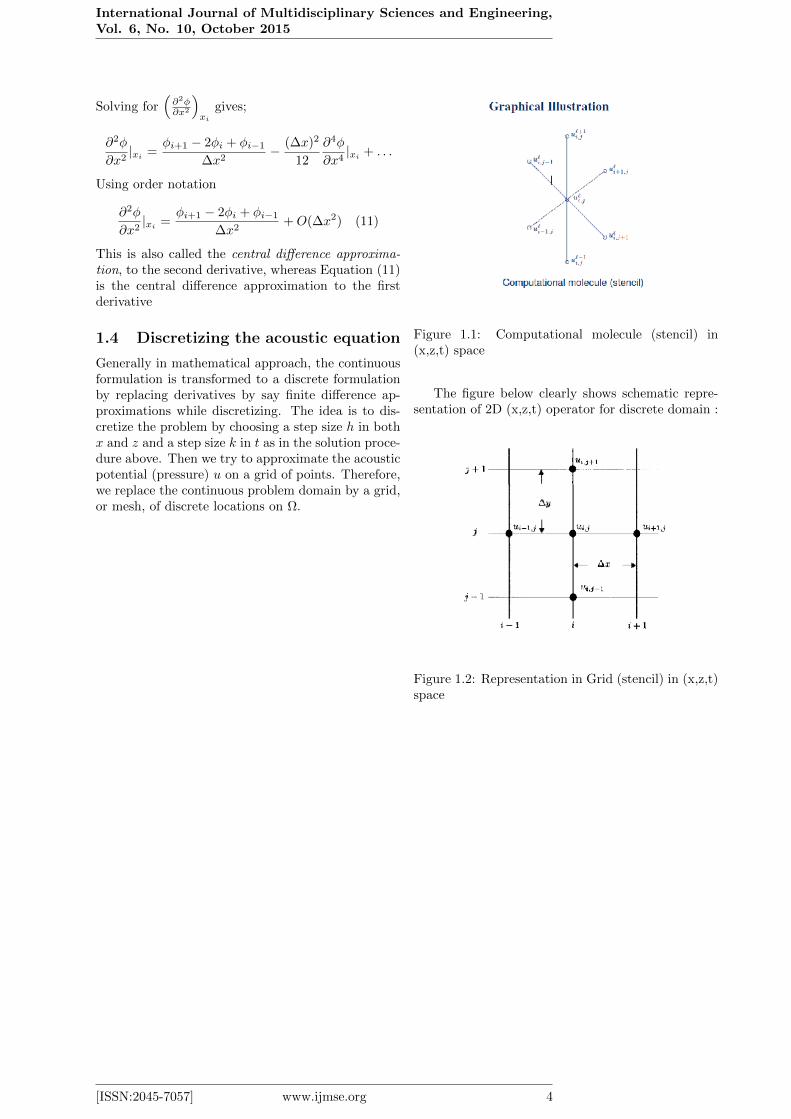
1.4 Discretizing the acoustic equation

Generally in mathematical approach, the continuousformulation is transformed to a discrete formulationby replacing derivatives by say finite difference ap-proximations while discretizing. The idea is to dis-cretize the problem by choosing a step size h in bothx and z and a step size k in t as in the solution proce-dure above. Then we try to approximate the acousticpotential (pressure) u on a grid of points. Therefore,we replace the continuous problem domain by a grid,or mesh, of discrete locations on Ω.

Figure 1.1: Computational molecule (stencil) in(x,z,t) space

The figure below clearly shows schematic repre-sentation of 2D (x,z,t) operator for discrete domain :

Figure 1.2: Representation in Grid (stencil) in (x,z,t)space



2 Numerical schemes

In this section, we develop the two numerical schemesthat we shall use in this study, that is Central Differ-ence Scheme (explicit) and Crank-Nicolson schemes(Hybrid) for the model equation

∂2u

∂x2+∂2u

∂z2− 1

c2(x, z)

∂2u

∂t2= S(x, z, t)

which is a hyperbolic PDE, therefore we first dis-cretize this equation by using the central differenceapproximation to the second derivative in uxx, uzzand utt

2.1 Central Difference Scheme(CDS)(Explicit)

Construction of the simple explicit scheme for thehomogeneous 2-dimensional acoustic wave equationin rectangular coordinate is a fairly straight forwardmatter. Namely;

utt = c2 (uxx + uzz) , (2.1)

where S = 0 which means that there is no supply ofenergy from the source. To develop explicit schemefor this equation, we discretize the terms in the homo-geneous equation governed by (2.1) in the standardway by defining the central difference operators asfollows:

D2xu

ni,j =

uni+1,j − 2uni,j + uni−1,j

(∆x)2

D2zuni,j =

uni,j+1 − 2uni,j + uni,j−1

(∆z)2

Substituting these operators in equation (2.1), we ar-rive at:

un+1i,j = 2uni,j − un−1

i,j + c2k2D2xu

ni,j + c2k2D2

zuni,j

Systematic substitution yields;

un+1i,j − 2uni,j + un−1

i,j

(∆t)2=

c2

(∆x)2

(uni+1,j − 2uni,j + uni−1,j

)+

c2

(∆z)2

(uni,j+1 − 2uni,j + uni,j−1

). (2.2)

We then express un+1i,j in terms of other terms to give;

un+1i,j = 2uni,j−un−1

i,j +c2(∆t)2

(∆x)2


)+

c2(∆t)2(∆z)2(uni,j+1 − 2uni,j + uni,j−1

)(2.3)

subscripts, i, j and superscript n represent the x, zand time co-ordinates respectively for a discrete gridof uniform spacing that is ∆x = ∆z and for con-

venience, we introduce the substitution σ =(c∆t∆x

)2,

this yields;

un+1i,j = 2uni,j − un−1

i,j + σ(uni+1,j − 2uni,j + uni−1,j

)+

σ(uni,j+1 − 2uni,j + uni,j−1

). (2.4)

therefore,

un+1i,j = (2− 4σ)uni,j + σuni+1,j + σuni−1,j+

σuni,j+1 + σuni,j−1 − un−1i,j . (2.5)

Using the same reasoning we can extend this conceptto non-homogeneous case below

uxx + uzz −1

c2(x, z)utt = S(x, z, t)

asc2i,j

(∆x)2


)+

c2i,j(∆z)2

(uni,j+1 − 2uni,j + uni,j−1

)−(


i,j

(∆t)2

)= c2i,jS

ni,j (2.6)

Again by letting σ =(ci,j∆t

∆x

)2

and subscripts, i, j

and superscript n to represent the x, z and time co-ordinates respectively for a discrete grid of uniformspacing that is ∆x = ∆z then, collecting the un-known terms that is un+1

i,j on the left hand side gives;

un+1i,j = (2− 4σ)uni,j+

σ(uni+1,j + uni−1,j + uni,j+1 + uni,j−1

)− un−1

i,j −

c2i,j∆t2Sni,j , (2.7)

which is the explicit scheme for the two dimensionalacoustic wave with source term for alli = 1, 2, 3, . . . ,M − 1; j = 1, 2, 3, · · · , N − 1.

2.2 Crank - Nicolson scheme

In Crank-Nicolson scheme, we replace the spatial co-ordinates uxx and uzz by the average of each centraldifference approximations at nth time level and at(n+ 1)th time level. These yields in (1.3.2) as

c2i,j2(∆x)2

[(un+1i+1,j − 2un+1

i,j + un+1i−1,j

)]+

c2i,j2(∆x)2

[(uni+1,j − 2uni,j + uni−1,j

)]+

c2i,j2(∆z)2

[(un+1i,j+1 − 2un+1

i,j + un+1i,j−1

)]+

c2i,j2(∆z)2

[(uni,j+1 − 2uni,j + uni,j−1

)]−(


i,j

k2

)= c2i,j

(Sni,j + Sn+1

i,j

)2

(2.8)



In order to reduce the computing time, we adopt uni-form grid spacing that is ∆x = ∆z = h and ∆t = k,

now letting r =c2i,j∆t

2

2∆x2 =c2i,jk

2

2h2 to give

c2i,jk2

2h2

[(un+1i+1,j − 2un+1

i,j + un+1i−1,j

)+(un+1i,j+1 − 2un+1

i,j + un+1i,j−1

)]+

c2i,jk2

2h2

[(uni+1,j − 2uni,j + uni−1,j

)+(uni,j+1 − 2uni,j + uni,j−1

)]−

un+1i,j + 2uni,j − un−1

i,j = c2i,jk2

(Sni,j + Sn+1

i,j

)2

(2.9)

on collecting unknown terms un+1i,j on the left hand

side gives the Implicit Crank-Nicolson scheme

−run+1i+1,j+(1+4r)un+1

i,j −run+1i−1,j−ru

n+1i,j+1−ru

n+1i,j−1 =

runi+1,j+(2−4r)uni,j+runi−1,j+ru

ni,j+1+runi,j−1−un−1

i,j −

c2i,jk2

(Sni,j + Sn+1

i,j

)2

, (2.10)

for alli = 1, 2, 3, · · · ,M − 1 and j = 1, 2, 3, · · · , N − 1Taking S to be a space function of x and z but nota function of time(t), then Sni,j = Sn+1

i,j , our ImplicitCrank-Nicolson equation reduces to

−run+1i+1,j+(1+4r)un+1


n+1i,j+1−ru

n+1i,j−1 =



i,j −

c2i,jk2Sni,j (2.11)

for all i = 1, 2, 3, · · · ,M−1; and j = 1, 2, 3, · · · , N−1

3 Results

Accuracy and Stability analysis

3.1 Matrix stability of Explicit scheme

Matrix stability method considers the finite differ-ence representation of both the PDE and boundarycondition in a matrix form for which eigenvalue anal-ysis is used to study stability, the theory behind thismethod is that the modulus of the eigenvalues of theamplification matrix should be less than unity. Em-ploying matrix method to analyze stability of thescheme (2.7)and expanding this scheme by takingi = 1, 2, 3, . . . ,M − 1; j = 1, 2, 3, . . . , N − 1, andr = σ = (

ci,j∆t∆x )2, generates the system of equations

(see appendix) which can be expressed in matrix formas

Un+1i,j = AUni,j − Un−1

i,j + b,

where

un+1i,j =

u1,1

u2,1

...u1,2

...uM−1,N−1

n+1

A =

(2− 4r) r · · · r

r (2− 4r) r · · · r...

. . .. . . · · ·

...· · · r · · · r (2− 4r)

uni,j =

u1,1

u2,1

...u1,2

...uM−1,N−1

n

b =

run0,1 + run1,0 + run0,1 − c21,1k2Sn1,1run2,0 − c22,1k2Sn2,1

...

and

un−1i,j =

u1,1

u2,1

...u1,2

...uM−1,N−1

n−1

We realise some pattern and the resulting matrix[(M − 1)× (N − 1)]× [(M − 1)× (N − 1)] is of block-tridiagonal form as

G =

C DB C D

. . .. . .

. . .

B C,

where B,C and D are (M − 1) × (M − 1) matrices,and there are N such C matrices on the diagonal. Forthis case, B and D are diagonal matrices whereas Cis tridiagonal,

C =

(2− 4r) r

r (2− 4r) r. . .

. . .. . .

r (2− 4r)

,

B = D =

r

r. . .

r

Since C is tridiagonal matrix which is symmetric pos-itive definite and is diagonally dominant, then C isnon-singular thus there is a unique solution. Thesymmetry then implies that we have both a neces-sary condition for stability, therefore this scheme willalways be stable for restricted values of r.

3.2 Von Neumann stability of Explicitscheme (CDS)

The von Neumann stability analysis is a way to deter-mine when a particular numerical method is stable.



It looks at solutions of the form anj = ξneijkh, where

i =√−1, j is our spatial index, k is the time index,

and h is the spatial step. To do the analysis usingthis method, we simply substitute the above solutioninto the discretized form of the numerical method anddetermine where | ξ |2≤ 1. This tells us whether theamplitude of the wave is less than or equal to one. Ifthe amplitude is greater than one, then the amplitudeis increasing and will therefore eventually become un-stable. Thus the method is stable at the values where| ξ |2≤ 1. In general, the Von Neumanns procedureintroduces an error represented by a finite Fourier se-ries and examines how this error propagates duringthe solution.Stability being independent of source term, now get-ting the stability of explicit scheme using Von Neu-mann’s method, we set S = 0 in the explicit scheme(2.7) to give the homogeneous equation;

un+1i,j = (2− 4σ)uni,j+

σ(uni+1,j + uni−1,j + uni,j+1 + uni,j−1

)− un−1

i,j (3.1)

Then using the fact that the solution of this con-stant coefficient differential equation is satisfied bythe Fourier harmonics

Uni,j = ξneiβmheiγlh.

whereβ is time index in xγ is time index in zh is spatial step in x and zm is spatial index in xand l is spatial index in z.Substituting in the homogeneous scheme (3.1), we get

ξn+1eiβmheiγlh = (2− 4σ)ξneiβmheiγlh+

σ[ξneiβ(m+1)heiγlh + ξneiβ(m−1)heiγlh

]+

σ[ξneiβmheiγ(l+1)h + ξneiβmheiγ(l−1)h

]−

ξn−1eiβmheiγlh (3.2)

so that on dividing equation (3.2) by ξneiβmheiγlh,we have;

ξ = (2− 4σ) + σ[eiβh + e−iβh + eiγh + e−iγh

]− ξ−1

But 2 cos θ = eiθ + e−iθ which reduces this equationto

ξ = (2−4σ)+σ

[2(1− 2 sin2 βh

2) + 2(1− 2 sin2 γh

2)

]−ξ−1 (3.3)

then;

ξ2 − 2

[1− 2σ(sin2 βh

2+ sin2 γh

2)

]ξ + 1 = 0

we then let g =[1− 2σ(sin2 βh

2 + sin2 γh2 )], to

get;ξ2 − 2gξ + 1 = 0,

where the ith eigenvalue is given by

ξi = g ±√g2 − 1

Therefore, for stability, | ξi |≤ 1; i = 1, 2, · · · , N ,this implies

−1 ≤ 1− 2σ(sin2 βh

2+ sin2 γh

2) ≤ 1

which has non-trivial solution when1− 2σ(sin2 βh

2 + sin2 γh2 ) ≥ −1,

for this we get;

σ(sin2 βh

2+ sin2 γh

2) ≤ 1,

since the maximum value of sin2 βh2 is unity, our

equation reduces to σ ≤ 12 as stability condition.

Therefore, convergence of the scheme follows the Courantet al. (1928) (C.F.L.) condition for convergence, whichapplies to explicit difference replacement of hyper-bolic equations. It requires that (3.1) to be conver-gent when 0 ≤ σ ≤ 1

2 . Thus, the stability conditioncoincides with the C.F.L. condition.

Crank-Nicolson scheme (Hybrid)

3.3 Matrix stability of Crank-Nicolsonscheme

Similarly, we adopt the matrix method to analyzestability of the Crank-Nicolson scheme (2.11). Weexpand this scheme by takingi = 1, 2, 3, · · · ,M − 1; j = 1, 2, 3, · · · , N − 1, toget the system of equations which we can express inmatrix form as

(1 + 4r) −r · · · −r−r (1 + 4r) −r · · ·...

. . .. . .

...−r · · · −r (1 + 4r)

−r · · · (1 + 4r)

u1,1

u2,1

...u1,2

...uM−1,N−1

n+1

=

(2− 4r) r · · · r

r (2− 4r) r · · · r...

. . .. . .

. . ....

r · · · r (2− 4r) rr · · · r (2− 4r)



u1,1

u2,1

...u1,2

...uM−1,N−1

n

+

run+10,1 + run+1

1,0 + run0,1 + run1,0 − un−11,1 − k2Sn1,1

run+12,0 + run2,0 − un−1

2,1 − k2Sn2,1...

run+10,2 + run0,2 − un−1

1,2 − k2Sn1,2...

.

Which we can express in matrix form as

AUn+1i,j = BUni,j + C

Un+1i,j = (A−1B)Uni,j + A−1C · · · (3.3a)

A and B are block tridiagonal matrices. Thus, equa-tion (3.3a) may be put in the form

(I − rAN−1)Un+1i,j = (2I + rAN−1)Uni,j + D,

where

AN−1 =

−4 1 0 · · · 01 −4 1 · · · 0

0 1 −4 1...

.... . . · · · 1 −4

0 · · · 0 · · · −4

I is an (N − 1)× (N − 1) identity matrix. Thus,

Un+1i,j =

[(2I + rAN−1)(I − rAN−1)−1

]Uni,j + E,

where D = A−1C and E = C(I − rAN−1)−1.In simpler form we write this equation as

Un+1i,j = PUni,j + E

In this case, P = (2I + rAN−1)(I − rAN−1)−1 isthe amplification matrix, and the stability conditionis that absolute value of the eigenvalues of the am-plification matrix should be less than or equal to 1,that is | λi |≤ 1. Since our Equation (2.11) is implicitand A and B are block tridiagonal matrices which aresymmetric positive definite and are weakly diagonallydominant, then A and B are non-singular thus thereis a unique solution, the symmetry then implies thatwe have both necessary and sufficient condition forstability, therefore this scheme will always be stablefor all values of r since r has no restrictions (uncon-ditionally stable).

3.4 Von Neumann stability of Crank-Nicolson scheme

To get stability of Crank Nicolson via this method,we set S = 0 since stability is independent of sourceterm, then substitute Uni,j = ξneiβmheiγlh in the ho-mogeneous equation (2.11)

−run+1i+1,j+(1+4r)un+1


n+1i,j+1−ru

n+1i,j−1 =



i,j ,(3.4)

which yields

−rξn+1eiβ(m+1)heiγlh + (1 + 4r)ξn+1eiβmheiγlh−

rξn+1eiβ(m−1)heiγlh − rξn+1eiβmheiγ(l+1)h

−rξn+1eiβmheiγ(l−1)h = rξneiβ(m+1)heiγlh+

(2− 4r)ξneiβmheiγlh + rξneiβ(m−1)heiγlh+

rξneiβmheiγ(l+1)h+rξneiβmheiγ(l−1)h−ξn−1eiβmheiγlh

(3.5)Again dividing (3.5) by ξneiβmheiγlh, we obtain

(1 + 4r)ξ − rξ(eiβh + e−iβh)− rξ(eiγh + e−iγh) =

(2−4r)+r(eiβh+e−iβh)+r(eiγh+e−iγh)−ξ−1 (3.6)

Recall that cos θ = 1 − 2 sin2 θ2 = eiθ+e−iθ

2 , thereforeusing this fact in (3.6), yields

(1+4r)ξ−rξ(

2(1− 2 sin2 βh

2) + 2(1− 2 sin2 γh

2)

)=

(2−4r)+r

(2(1− 2 sin2 βh

2) + 2(1− 2 sin2 γh

2)

)− 1

ξ

After rearrangement, we get

ξ2

[1 + 4r(sin2 βh

2+ sin2 γh

2)

]

−ξ[2− 4r(sin2 βh

2+ sin2 γh

2)

]+ 1 = 0

which has a non-trivial solution when −1 ≤ ξi ≤ 1,where ξi is the magnification factor corresponding toeigenvalue, thus;

ξi =2− 4r(sin2 βh

2 + sin2 γh2 )

2 + 8r(sin2 βh2 + sin2 γh

2 )≤ 1

Now for | ξi |≤ 1, we have sin2 βh2 = 1 and

sin2 γh2 = 1, therefore

ξi =1− 4r

1 + 8r

Hence for stability r > 0, which makes ξi less thanunity for all values of r implying unconditional sta-bility throughout.



Analysis and Software

In this section we present an analysis of the numericalexperiments. We also present and discuss the resultsobtained from these methods. We shall display theseresults using three- dimensional figures and graphs.

From the initial condition

ut(x, z, 0) = 0

But since ut is approximated using central differencei.e. (??), then central difference analogue of ut yields

ut ≈un+1i,j − u

n−1i,j

2k= 0

Taking n = 0, from initial condition we find

ut ≈u0+1i,j − u

0−1i,j

2k= 0,

wherek = ∆t

Implying thatu1i,j = u−1

i,j

Again, from the initial condition, u(x, z, 0) = (sinπx)(sinπz),we get that

u(x, z, 0) ≈ u0i,j = (sinπx)(sinπz)

At this point we developed a Matlab program thatcould give the pressure field as a function of x and zat varying time levels and results have been plottedfor both equation (2.7) and (2.11).

Figure 3.1: Numerical solution explicit scheme atc=1500,dt=0.5

Figure 3.2: Numerical solution Crank Nicolsonscheme at c=1500,dt=0.5



Figure 3.3: numerical solution of explicit scheme att=10,c=1500.dt=0.5

Figure 3.4: numerical solution of Crank Nicolsonscheme at t=10,c=1500.dt=0.5

4 Discussions

In reality, sound propagation in elastic medium isdamped, the amplitude of the pressure of the soundwave decreases with increasing distance from the soundsource. Our results from the two numerical schemes(CDS) and (CNS) are confirming this since the dis-placement of the particles given by u(x, z, t) is de-creasing with an increase in the distance from thesource (in this case t=0). The efficacy of a finite dif-ference scheme is achieved with the increase of thegrid points involved hence the increase in the accu-racy of a finite difference scheme. In addition, thespeed of sound reduces with increase in the distancefrom the source, this is evidenced by the reductionof the ripples as the propagation advances away fromsource see figure 4.1.3.

Conclusions

This study focussed on the second order acoustic equa-tion with a signal function. Two numerical schemesnamely Central Difference Scheme (Explicit scheme)and Hybrid scheme (Crank Nicolson Scheme) were

Figure 3.5: Numerical solution explicit scheme atc=1000,dt=0.8

Figure 3.6: Numerical solution Crank Nicolsonscheme at c=1000,dt=0.8

developed and used in this study. The stability anal-yses of the developed schemes revealed that Explicitscheme was conditionally stable while the Hybrid one(Crank Nicolson Scheme) was unconditionally stable,for all values of courant number r.The rate of convergence of the algorithms depends onthe truncation error introduced when approximatingthe partial derivatives, the Crank-Nicolson methodconverges at the rate of (k2 + h2), which is a fasterrate of convergence than either the explicit method,or the implicit method. Further, since c is a functionof (x, z), from the results it suffices to use the maxi-mum sound velocity in the model.The smaller the mesh sizes, the more finely the re-sults, this makes the grid more finer thus improvingthe approximation around the boundary but at thecost of strongly increased computational time as evi-denced by figures (4.1.5, 4.1.6).

5 Recommendations

We wish to recommend that further research can beundertaken to;



Figure 3.7: Numerical solution explicit scheme att=5,c=0.5,dt=0.5

(1).png

Figure 3.8: Numerical solution Crank Nicolsonscheme at t=5,c=0.5,dt=0.5

(i) Explore numerical solution to this problem us-ing other methods like finite element and com-pare results.

(ii) Try out an analytical method via green’s func-tion.

References

[1] Alford, R. M., Kelly, K. R., and Boore, D. M.(1974): Accuracy of finite-difference model-ing of acoustic wave propagation, Geophysics,vol. 39, pp 834-842.

[2] Alford, R. M., Kelly, K. R., and Boore, D. M.(1974): Accuracy of finite-difference model-ing of acoustic wave propagation, Geophysics,vol. 39, pp 834-842.

[3] Bernatz, R. (2010): Fourier series and numer-ical methods for partial differential equations,Luther College, John Wiley & Sons, inc., publi-cation.

[4] Borthen, J. (2010): A numerical approximationof the wave equation, Mathematics and Statis-tics, Georgetown University.

[5] Brekhovskikh, L. M., and Yu Lysanov, P. (2003):Fundamentals of Ocean Acoustics, 3rd edition,Springer-Verlag, NY.

[6] Cerjan, C., Kosloff, D., Kosloff, R., and Reshef,M. (1985): A nonreflecting boundary conditionfor discrete acoustic and elastic wave equations,Geopgysics, vol. 50, no. 4, pp.705-708.

[7] Charara, M. and Tarantola, A. (1996):Boundary conditions and the source termfor one-way acoustic depth extrapolation,Geophysics,vol. 61 , pp 244-252.

[8] Clay, C. S., Medwin, H. (1977): Acousti-cal Oceanography: Principles and Applications,John Wiley and Sons, New York, NY, pp. 88 and98-99.

[9] Daniel, R. R. (2009): The science and Applica-tion of acoustics second edition, The City Collegeof the City University of New York.

[10] David, H. and Robert, R. (1989): Fundamentalof physics, 2nd Edition, John Wiley and sons,New York.

[11] Evans, C. L. (1997): Partial Differential Equa-tions, American Mathematical Society.

[12] Frank J. F. (2000): Foundations of engineer-ing acoustics, Institite of sound and vibrationresearch, University of Southampton, U.K.

[13] Hugh D. G. and Pat, F. D. (2003): Finite differ-ence modelling of the full acoustic wave equationin Matlab, CREWES Research Report vol. 15.

[14] Jain, M. K. (1991): Numerical solution of Dif-ferential Equations, Wiley Eastern Limited, NewDelhi.

[15] Jensen, F., Kuperman, W., Porter, M., andSchmidt, H. (2000): Computational OceanAcoustics, springer, New York, pp.11-12 and 52-54.

[16] John, H. M. (2001): Numerical Methods forMathematics, Science and Engineering,2nd Edi-tion, Prentice Hall of India. New Delhi.

[17] Kelly, K. R., Ward, R. W., Sven T. andAlford, R. M. (1976): Synthetic Seismo-grams: A finite-difference Approach, Geo-physics, vol. 41, no. 1, p.2-27.

[18] Lines, L. R. Slawinski, R. and Bording, R. P.(1999): A recipe for stability of finite differ-ence wave equation computations, Geophysics,vol. 64, pp 967-969.



[19] Maarten, V. W. and Kowalczyk, K. (2008): Onthe numerical solution of the 2D wave equa-tion with compact FDTD schemes, Sonic ArtsResearch Centre, Queen’s University Belfast,United Kingdom.

[20] Randall. J. L. (2005): Finite difference Meth-ods for Differential Equations, lecture notes forAmath 585-586 University of Washington.

[21] Rao, S. K. (2004): Introduction to Partial Dif-ferential Equations, Prentice Hall of India, NewDelhi.

[22] Richtmyer, R. D. and Morton, K. W. (1967):Tridiagonal Algorithm, Lecture notes.

[23] Rodney, F. W. C. (1990): Underwater acousticsystems, John Wiley and sons, New York.

[24] Seongjai, K. (2002): Higher-Order Schemes forAcoustic Waveform Simulation, Acoustic Wave-form Simulation , Department of Mathematics,University of Kentucky, Lexington, Kentucky40506-0027 USA, March.

[25] Serway, R. A. and Faughn, J. S. (1992): Stu-dent Solutions, Manual and Study Guide to ac-company College Physics, 4th Edition. Saunderscollege Publishing.

[26] Strikwerda, J. C. (1989): Finite Differ-ence Schemes and Partial Differential Equa-tions, Wadsworth and Brook/Cole.

[27] Vetreno, J. R. (2007): Analytic Models forAcoustic Wave Propagation in Air, Master’sThesis, North Carolina State University.

[28] William, F. A. (1992): Numerical methods forpartial differential equations, third edition, Aca-demic press, New York.

[29] Xie, X. B., and Wu, R.S. (1997): Free surfaceboundary condition and the source term for one-way elastic wave method, Institute of Tectonics,University of California, Santa Crux.



6 Appendix

6.1 Matrix Generation

Set one, j = 1;

un+11,1 = run2,1 + (2− 4r)un1,1 + run0,1 + run1,2 + run1,0 − c21,1(∆t)2Sn1,1 − un−1

1,1


2,1


3,1

... =...

...

un+1M−1,1 = runM,1 + (2− 4r)unM−1,1 + runM−2,1 + runM−1,2 + runM−1,0−

c2M−1,1(∆t)2SnM−1,1 − un−1M−1,1

In set two, we set j = 2 to generate the systems of equations


1,2


2,2


3,2

... =...

...


c2M−1,2(∆t)2SnM−1,2 − un−1M−1,2

Continuing in the same trend, we set j = 3 to give


1,3


2,3


3,3

... =...

...


c2M−1,3(∆t)2SnM−1,3 − un−1M−1,3

Setting j = 4 yields


1,4


2,4


3,4


4,4

... =...

...


c2M−1,4(∆t)2SnM−1,4 − un−1M−1,4



This process is continued until i = (M − 1), j = (N − 1) as below

un+11,N−1 = run2,N−1 + (2− 4r)un1,N−1 + run0,N−1 + run1,N + run1,N−2−

c21,N−1(∆t)2Sn1,N−1 − un−11,N−1


c22,N−1(∆t)2Sn2,N−1 − un−12,N−1


c23,N−1(∆t)2Sn3,N−1 − un−13,N−1

... =...

...

un+1M−1,N−1 = runM,N−1 + (2− 4r)unM−1,N−1 + runM−2,N−1 + runM−1,N + runM−1,N−2−

c2M−1,N−1(∆t)2SnM−1,N−1 − un−1M−1,N−1

6.2 Matlab Programme


Documents

Finite Di erence Analysis of 2-Dimensional Acoustic Wave ... · Finite Di erence Analysis of 2-Dimensional Acoustic Wave with a Signal Function Opiyo Richard Otieno 1, ... two dimensional