This article was downloaded by: [The UC Irvine Libraries]On: 17 October 2014, At: 02:01Publisher: RoutledgeInforma Ltd Registered in England and Wales Registered Number: 1072954 Registered office: Mortimer House,37-41 Mortimer Street, London W1T 3JH, UK

Applied Financial EconomicsPublication details, including instructions for authors and subscription information:http://www.tandfonline.com/loi/rafe20

Financial market spillovers around the globeThomas Dimpfl a & Robert C. Jung ba Wirtschafts- und Sozialwissenschaftliche Fakultät , Eberhard Karls Universität Tübingen ,Mohlstr. 36, D-72074 Tübingen, Germanyb Staatswissenschaftliche Fakultät , Universität Erfurt , D-99089 Erfurt, GermanyPublished online: 27 Sep 2011.

To cite this article: Thomas Dimpfl & Robert C. Jung (2012) Financial market spillovers around the globe, Applied FinancialEconomics, 22:1, 45-57, DOI: 10.1080/09603107.2011.597721

To link to this article: http://dx.doi.org/10.1080/09603107.2011.597721

PLEASE SCROLL DOWN FOR ARTICLE

Taylor & Francis makes every effort to ensure the accuracy of all the information (the “Content”) containedin the publications on our platform. However, Taylor & Francis, our agents, and our licensors make norepresentations or warranties whatsoever as to the accuracy, completeness, or suitability for any purpose of theContent. Any opinions and views expressed in this publication are the opinions and views of the authors, andare not the views of or endorsed by Taylor & Francis. The accuracy of the Content should not be relied upon andshould be independently verified with primary sources of information. Taylor and Francis shall not be liable forany losses, actions, claims, proceedings, demands, costs, expenses, damages, and other liabilities whatsoeveror howsoever caused arising directly or indirectly in connection with, in relation to or arising out of the use ofthe Content.

This article may be used for research, teaching, and private study purposes. Any substantial or systematicreproduction, redistribution, reselling, loan, sub-licensing, systematic supply, or distribution in anyform to anyone is expressly forbidden. Terms & Conditions of access and use can be found at http://www.tandfonline.com/page/terms-and-conditions

Applied Financial Economics, 2012, 22, 45–57

Financial market spillovers around

the globe

Thomas Dimpfla,* and Robert C. Jungb

aWirtschafts- und Sozialwissenschaftliche Fakultat, Eberhard Karls

Universitat Tubingen, Mohlstr. 36, D-72074 Tubingen, GermanybStaatswissenschaftliche Fakultat, Universitat Erfurt, D-99089 Erfurt,

Germany

This article investigates the transmission of return and volatility spillovers

around the globe. It draws on index futures of three representative indices,

namely the Dow Jones Euro Stoxx 50, the S&P 500 and the Nikkei 225.

Devolatized returns and realized volatilities are modelled separately using

a Structural Vector Autoregressive (SVAR) model, thereby accounting for

the particular sequential time structure of the trading venues. Within this

framework, we test hypotheses in the spirit of Granger causality tests,

investigate the short-run dynamics in the three markets using Impulse

Response (IR) functions, and identify leadership effects through variance

decomposition. Our key results are as follows. We find weak and short-

lived return spillovers, in particular from the USA to Japan. Volatility

spillovers are more pronounced and persistent. The information from the

home market is most important for both returns and volatilities; the

contribution from foreign markets is less pronounced in the case of returns

than in the case of volatility. Possible gains in terms of forecasting

precision when applying our modelling strategy are illustrated by a forecast

evaluation.

Keywords: spillovers; index futures; realized volatility; structural

VAR model

JEL Classification: C32; G15

I. Introduction

This article investigates the correlation dynamics of

stock index returns and volatility in the three major

financial centres around the globe: Asia, Europe and

the United States. It continues a strand of the

literature in empirical finance that goes back to the

seminal papers of Hamao et al. (1990), Lin et al.

(1994) and Susmel and Engle (1994), if not further,

and builds upon the quite distinctive definition of

spillovers developed therein. Unfortunately, there is

no generally agreed upon definition of spillovers in

the financial literature and therefore, the closely

related concepts ‘spillover’, ‘contagion’, ‘interdepen-

dence’ and ‘comovement’ are often used interchange-

ably. Gallo and Otranto (2008) provide a clarificatory

discussion of these terms and attempt to establish

some practical definitions. Following, first and

*Corresponding author. E-mail: thomas.dimpfl@uni-tuebingen.de

Applied Financial Economics ISSN 0960–3107 print/ISSN 1466–4305 online � 2012 Taylor & Francis 45http://www.tandfonline.com

http://dx.doi.org/10.1080/09603107.2011.597721

Dow

nloa

ded

by [

The

UC

Irv

ine

Lib

rari

es]

at 0

2:01

17

Oct

ober

201

4

foremost, Hamao et al. (1990), return and volatilityspillovers are defined in the present study to be effectsfrom foreign stock markets on the conditional meansand variances of daytime returns of subsequentlytrading markets. As has already been pointed out byHamao et al. (1990), this particular concept ofspillovers requires the use of intraday data to dividedaily (close-to-close) returns into daytime (open-to-close) and overnight (close-to-open) returns.Subsequent work such as that of Baur and Jung(2006) and Soriano and Climent (2006) stresses theimportance of this partitioning.

Classic financial theory, like the (strong-form)efficient market hypothesis, predicts that returnspillovers do not occur, as the information frompreviously trading markets should be fully reflected inthe overnight returns. However, there is ampleempirical evidence that stock markets do notinstantly incorporate all overnight information intothe opening prices, see e.g. Hamao et al. (1990), Linet al. (1994), Baur and Jung (2006) and Savva et al.(2009). Explanations for this empirical phenomenoncan be found in the literature on asset valuationmodels, such as Kyle (1985) and Admati andPfleiderer (1988), and in the behavioural financeliterature. According to the former body of literature,traders may not yet perceive the entire informationcontent of previous trading in foreign markets, and,thus, be unwilling to fully trade their demandschedule and thereby reveal their share of privateinformation. Therefore, the full incorporation ofnewly arriving information might take time and,thus, might cause spillovers into the daytime returnsof the domestic market. In this context, spillovers arean expression of valuation insecurity, but not marketinefficiency and are caused by the rational actions ofagents. The behavioural finance literature has devel-oped several psychological explanations for the exis-tence of mean spillovers (see Fung et al., 2010, andthe literature cited therein).

In contrast to mean spillovers, the existence ornonexistence of volatility spillovers is an issue withregard to which classic financial theory has remainedrather silent. An extensive empirical literature hasprovided ample evidence of (short-lived) volatilityspillovers from foreign stock markets into domesticones. The article by Soriano and Climent (2006)provides a useful survey, while Melvin and PeiersMelvin (2003) discuss different sources of volatilityspillovers in the context of the closely relatedexchange rate markets. Diebold and Yilmaz (2009)and Harrison and Moore (2009) are recent contribu-tions which investigate international volatilitydynamics and spillovers. While their approaches arequite distinct from ours, their general results, namely

the detection of foreign volatility influences on home

market volatility, are in line with the results of this

article.On a more general level, the financial economics

literature has developed a number of theoretical

foundations with regard to the interdependence of

international stock markets. See, for example, Ge�bkaand Serwa (2007) for an overview and Pritsker (2001)

for an extensive discussion of transmission channels

from one market to the other.In the present article we propose separate

Structural Vector Autoregressive (SVAR) models

for stock index future returns and a suitable volatility

measure which enable us to test various hypotheses in

the spirit of Granger causality testing. Within this

framework we are able to use Impulse Response (IR)

functions to analyse short-run dynamics in the system

of global financial markets. Finally, we are able to

adopt variance decomposition to identify leadership

effects in both the mean and volatility systems. The

three major financial centres around the globe are

represented by the Nikkei 225 future for Asia, the

Dow Jones Euro Stoxx 50 future for Europe and the

S&P 500 future for the United States. The structure in

our model follows naturally from the timing of the

trading in these three markets and requires us to

model returns and volatility separately, as is done by,

for example, Diebold and Yilmaz (2009). As a

volatility measure we employ the realized volatilities

as suggested by Andersen et al. (2003). To overcome

the widely documented stale quote problem, we base

the empirical analysis on index future data instead of

the underlying indices, as is done, for example, by

Ryoo and Smith (2004).We proceed as follows. Section II discusses the

methodology employed in our empirical analysis, and

Section III describes the data. Section IV presents the

empirical results, while Section V provides the results

of an illustrative out-of-sample forecast and, finally,

Section VI concludes.

II. Methodology

The first part of this section describes the

generic multivariate modelling framework proposed

here for the analysis of return and volatility

spillovers, the structure of which results directly

from the opening and closing of the markets consid-

ered in this study. In the second part, details of the

specific return and volatility measurement employed

are presented.

46 T. Dimpfl and R. C. Jung

Dow

nloa

ded

by [

The

UC

Irv

ine

Lib

rari

es]

at 0

2:01

17

Oct

ober

201

4

Trading times and the econometric model

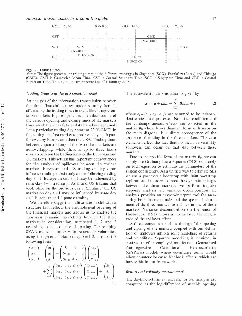
An analysis of the information transmission between

the three financial centres under scrutiny here isaffected by the trading times in the different represen-

tative markets. Figure 1 provides a detailed account ofthe various opening and closing times of the markets

from which the index futures data have been acquired.Let a particular trading day t start at 23:00 GMT. In

this setting, the first market to trade on day t is Japan,followed by Europe and then the USA. Trading times

between Japan and any of the two other markets arenonoverlapping, while there is up to three hours

overlap between the trading times of the European andUS markets. This setting has important consequences

for the analysis of spillovers between the variousmarkets: European and US trading on day t can

influence trading in Asia only on the following trading

day tþ 1. Europe on day tþ 1 may be influenced bysame-day tþ 1 trading in Asia, and US trading that

took place on the previous day t. Similarly, the USmarket on day tþ 1 may be influenced by same-day

tþ 1 European and Japanese trading.We therefore suggest a multivariate model with a

structure that reflects the chronological ordering of

the financial markets and allows us to analyse theshort-run dynamic interactions between the three

markets in consideration, numbered 1, 2 and 3according to the sequence of opening. The resulting

SVAR model of order p for returns or volatilities,using the generic notation xi,t, i¼ 1, 2, 3, is of the

following form:

x1,t

x2,t

x3,t

0B@

1CA¼

a1

a2

a3

0B@

1CAþ

0 0 0

b21,0 0 0

b31,0 b32,0 0

0B@

1CA

x1,t

x2,t

x3,t

0B@

1CA

þXpl¼1

b11,l b12,l b13,l

b21,l b22,l b23,l

b31,l b32,l b33,l

0B@

1CA

x1,t�l

x2,t�l

x3,t�l

0B@

1CAþ

"1,t

"2,t

"3,t

0B@

1CAð1Þ

The equivalent matrix notation is given by

xt ¼ aþ B0xt þXpl¼1

Blxt�l þ et ð2Þ

where et¼ ("1,t, "2,t, "3,t)0 are assumed to be indepen-

dent white noise processes. Note that coefficients ofthe contemporaneous effects are collected in thematrix B0 whose lower diagonal form with zeros onthe main diagonal is a direct consequence of thesequence of trading in the three markets. The zeroelements reflect the fact that no mean or volatilityspillovers can occur on that day between thesemarkets.

Due to the specific form of the matrix B0, we cansimply use Ordinary Least Squares (OLS) separatelyon each equation to estimate the parameters of thesystem consistently. As a unified way to estimate SEswe use a parametric bootstrap with 1000 bootstrapreplications. In order to trace the dynamic linkagesbetween the three markets, we perform impulseresponse analysis and variance decomposition. IRanalysis provides an easy-to-interpret tool for mea-suring both the magnitude and the speed of adjust-ment of the three markets to a shock in one of thesemarkets. Variance decomposition (in the sense ofHasbrouck, 1991) allows us to measure the magni-tude of the spillover effect.

A direct consequence of the timing of the openingand closing of the markets coupled with our defini-tion of spillovers inhibits joint modelling of returnsand volatilities. Separate modelling is required, incontrast to often employed multivariate GeneralizedAutoregressive Conditional Heteroscedastic(GARCH) models where covariance terms wouldallow counter-clockwise feedback effects, which areimpossible in our framework.

Return and volatility measurement

The daytime returns ri,t relevant for our analysis arecomputed as the log-difference of suitable opening

GMT

CST

SGT

CET

23:55 23:5552:6 00:8 14:30 21:0012:00

SGX SGX

EUREX

CME

7:55-10.1511:15-14:25

9:00-22.00

8:30-15:15

Fig. 1. Trading timesNotes: The figure presents the trading times at the different exchanges in Singapore (SGX), Frankfurt (Eurex) and Chicago(CME). GMT is Greenwich Mean Time, CST is Central Standard Time, SGT is Singapore Time and CET is CentralEuropean Time. Trading hours are presented as of 1 January 2006.

Financial market spillovers around the globe 47

Dow

nloa

ded

by [

The

UC

Irv

ine

Lib

rari

es]

at 0

2:01

17

Oct

ober

201

4

and closing transaction prices. Specific details con-cerning the different markets are given in Section III.To account for the presence of conditional hetero-scedasticity in the return time series we rely uponso-called ‘devolatized returns’, computed as daytimereturns ri,t standardized by the corresponding realizedvolatility �i,t (as defined below), following the recentproposal of Pesaran and Pesaran (2010). Formally,they are computed as

~ri,t ¼ri,t�i,t

ð3Þ

As shown by Pesaran and Pesaran (2010), devolatizedreturn series are approximately Gaussian andhomoscedastic.

We consider two different approaches that may befollowed in constructing the volatility time series: therealized volatility measure as proposed by Andersenet al. (2003), and the daily volatility estimate devel-oped by Bollen and Inder (2002) (subsequentlylabelled ABDL and BI, respectively). Both methodsseek to overcome the well-documented market micro-structure effects present in high-frequency financialdata when estimating the unobservable volatilityprocess.

Andersen et al. (2010) propose that the trueunderlying volatility process be estimated by sum-ming squared intraday returns computed over suit-ably large time intervals D. Specifically, they definethe daily realized variance on day t as

�2i,t ¼X1=Dj¼1

r2i,t,Djð4Þ

where ri,t,Djis the return computed over the intraday

time interval Dj and1D defines the number of intervals

used for calculating the volatility measures. Andersenet al. (2010) argue that due to market microstructurefrictions it is undesirable to sample returns infinitelyoften (i.e. D! 0), as would be required to approachthe true underlying volatility. When summing thesquared returns, one would at the same time accu-mulate the noise present in the market, which wouldlead to non-trivial measurement errors. To overcomethis issue, Andersen et al.’s (2003) realized volatility iscalculated using returns computed over sufficientlylarge time intervals D. For the subsequent applicationwe have chosen to use 5-minute returns for thecalculation of the realized variance in Equation 4,as done, for example, by Andersen et al. (2006).The realized volatility is then given by thesquare-root of �2i,t.

A drawback of using returns computed over5-minute intervals is the possible loss of informationcontained in the observations within the interval.Bollen and Inder (2002) therefore propose aVARHAC estimator in order to explicitly accountfor the different autocorrelation structures in intra-day returns induced by market microstructure effects.Specifically, they estimate for each trading day t anautoregressive model of order qt,

ri,t,Dj¼Xqtl¼1

�l,t ri,t,Dj�lþ �t,Dj

where �l,t denotes the autocorrelation parameter(s)and �t,Dj

are independent and identically distributed(i.i.d) errors. The optimal lag length per day qt ischosen by an information criterion. The purpose ofthis procedure is to purge the returns of microstruc-ture noise. The estimate of the daily volatility is thencomputed as

�2i,t ¼RSSi,t

1�Xqtl¼1

�l,t

" #2

RSSi,t ¼Xnt

j¼qtþ1

ri,t,Dj�Xqtl¼1

�l,t ri,t,Dj�l

!2

ð5Þ

and nt is the number of observations per day t. Theestimator in Equation 5 is efficient in the sense that itutilizes the data at the highest available frequency(1 minute for the data set at hand).

To model the volatility transmission between thethree major financial centres around the globe, wefollow Andersen et al. (2006), who suggest that thederived volatility time series be treated as if it weredirectly observed. This allows the straightforwardapplication of standard estimation techniques.

III. Data Description

The data set on which our analysis is based consists ofintraday transaction prices of the Dow Jones EuroStoxx 50 future (traded at Eurex), the S&P 500 future(traded at the Chicago Mercantile Exchange, CME)and the Nikkei 225 future (traded at the SingaporeExchange, SGX1). The datasets were obtained fromOlsen Financial Technologies and are sampled inminutes. Subsequently, we employ the followingacronyms for the future data from these three

1We use the Nikkei 225 future as traded at the SGX, as during the time period at hand the SGX was the market with thehighest trading volume of Nikkei 225 futures.

48 T. Dimpfl and R. C. Jung

Dow

nloa

ded

by [

The

UC

Irv

ine

Lib

rari

es]

at 0

2:01

17

Oct

ober

201

4

markets: FESX for the Eurex data, FSP for the CMEdata and FNI for the SGX data. The data coverfutures contracts from 1 July 2002 to 31 May 2006,and all futures are denominated in local currencies.The model is estimated using data up to andincluding 18 May 2006; the remaining days are usedto evaluate the out-of-sample forecast.

Previous studies dedicated to spillover analysis,such as Lin et al. (1994) and Baur and Jung (2006),have used indices instead of futures. The use of stockmarket indices, however, could entail the so-calledstale quote problem (cf. Ryoo and Smith, 2004). Toovercome this problem, it has been proposed that asuitable proxy be used for the opening quote of thestock index, varying from opening plus 5 minutes intothe trading day up to opening plus 30 minutes. Thisstrategy, however, might dilute the results in the sameway as the stale quote problem: prices of someunderlying stocks might already have changed sub-stantially within these 5 to 30 minutes. The approx-imate opening quote would then again not reflect thetrue opening index value. Using index future datahelps to overcome the stale quote problem withoutloss of information from the market opening. Indexfutures are self-contained securities and, thus, the firsttransaction in the morning of a new trading day isdriven only by information available to the market atthis point in time. A slight drawback of using futuresis that a continuous dataset is not available for a timehorizon greater than 9 months. So in order to obtaina continuous sample, we construct the return andvolatility time series for each future contract and rollover to the contract closest to maturity. The lasttrading day is excluded in order to avoid thepossibility of the settlement having an influence.

Essential for our analysis of spillover effects is thecalculation of returns and volatilities based onnonoverlapping trading hours. Trading at the SGXstarts at 7:55 and ends at 14:25 Singapore Time(SGT) and did not change throughout the 4 yearsunder study. As there is no overlap in trading timesbetween the SGX and the CME or between the SGXand Eurex (see Fig. 1), we compute the log-returns forthe FNI as open-to-close returns and the volatilitymeasures for the full trading day.

The FESX was traded at Eurex from 9:00 to 20:00Central European Time (CET) until 20 November2005. From 21 November 2005 on, Eurex extendedtrading hours from 9:00 to 22:00 CET. The FSP istraded in Chicago from 8:30 to 15:15 CentralStandard Time (CST) throughout our samplingperiod. Thus, there is an overlap of up to 6.5 hoursof trading between the two exchanges.

In order to obtain a clear-cut time structure, weapply the ideas of Menkveld et al. (2007) and Susmeland Engle (1994), who suggest that the intradayobservation period is restricted according to econom-ically relevant points in time. We choose to truncatethe FESX at 13:30 CET, well in advance of potentialmacroeconomic news announcements made in theUSA ahead of trading.2 The reason for this choice isthe assumption that European morning trade shouldconvey information which is of interest for the tradersin the United States and accounted for as soon astrading opens. We therefore compute the return andthe volatility measures of the FESX from the marketopening to 13:30 CET. The respective measures forthe FSP are computed from the opening to the closeof the CME.

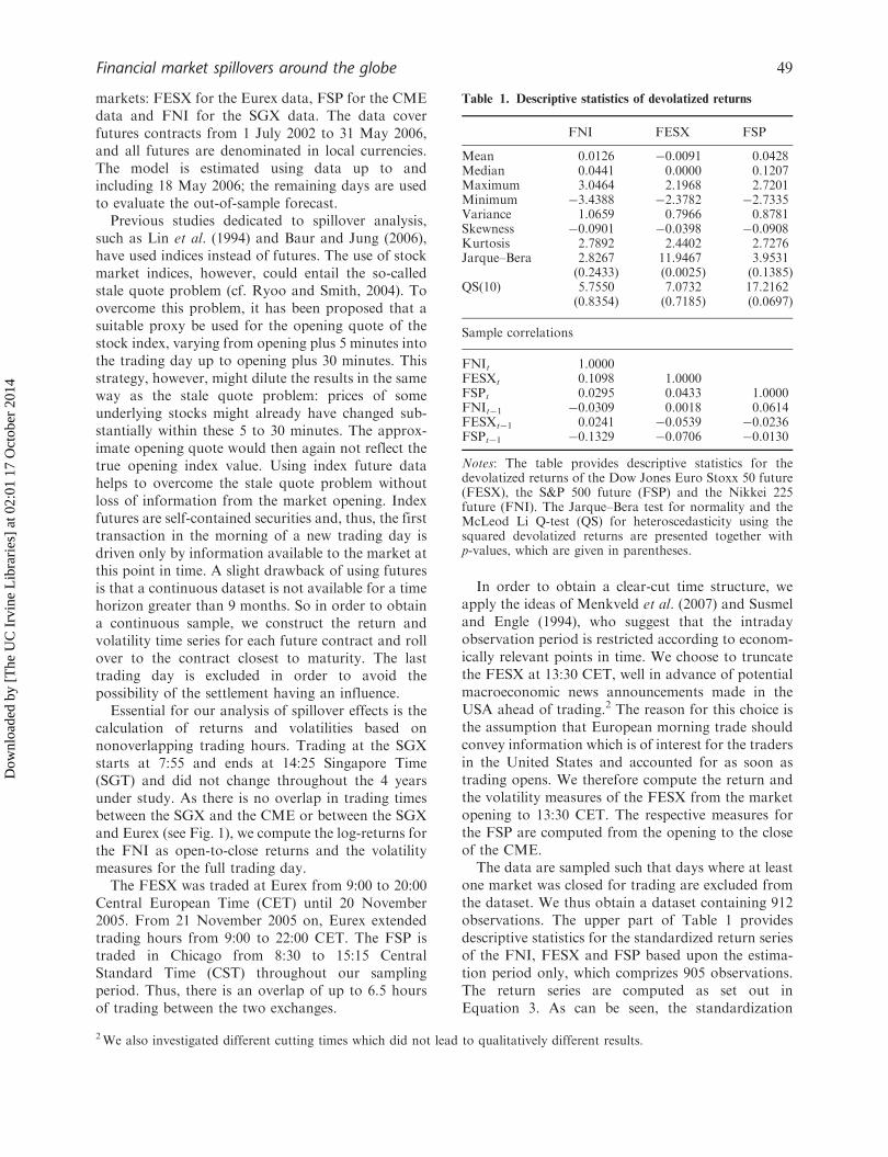
The data are sampled such that days where at leastone market was closed for trading are excluded fromthe dataset. We thus obtain a dataset containing 912observations. The upper part of Table 1 providesdescriptive statistics for the standardized return seriesof the FNI, FESX and FSP based upon the estima-tion period only, which comprizes 905 observations.The return series are computed as set out inEquation 3. As can be seen, the standardization

Table 1. Descriptive statistics of devolatized returns

FNI FESX FSP

Mean 0.0126 �0.0091 0.0428Median 0.0441 0.0000 0.1207Maximum 3.0464 2.1968 2.7201Minimum �3.4388 �2.3782 �2.7335Variance 1.0659 0.7966 0.8781Skewness �0.0901 �0.0398 �0.0908Kurtosis 2.7892 2.4402 2.7276Jarque–Bera 2.8267 11.9467 3.9531

(0.2433) (0.0025) (0.1385)QS(10) 5.7550 7.0732 17.2162

(0.8354) (0.7185) (0.0697)

Sample correlations

FNIt 1.0000FESXt 0.1098 1.0000FSPt 0.0295 0.0433 1.0000FNIt�1 �0.0309 0.0018 0.0614FESXt�1 0.0241 �0.0539 �0.0236FSPt�1 �0.1329 �0.0706 �0.0130

Notes: The table provides descriptive statistics for thedevolatized returns of the Dow Jones Euro Stoxx 50 future(FESX), the S&P 500 future (FSP) and the Nikkei 225future (FNI). The Jarque–Bera test for normality and theMcLeod Li Q-test (QS) for heteroscedasticity using thesquared devolatized returns are presented together withp-values, which are given in parentheses.

2We also investigated different cutting times which did not lead to qualitatively different results.

Financial market spillovers around the globe 49

Dow

nloa

ded

by [

The

UC

Irv

ine

Lib

rari

es]

at 0

2:01

17

Oct

ober

201

4

leaves the time series slightly mesokurtic. The Jarque–Bera test indicates that for two of the three series(FNI and FSP) the normality assumption can berejected only at the 1% level. Overall, the standardi-zation of the returns leads to time series which areapproximately Gaussian. For illustrative purposes wehave also employed McLeod and Li’s (1983) Q-test,which uses the squared devolatized returns to checkfor conditional heteroscedasticity. The p-values dis-played in Table 1 indicate no rejection of the nullhypothesis of conditional homoscedasticity for allthree series. The bottom part of Table 1 presentssample autocorrelations and (lagged) cross-correla-tions between the FNI, FESX and FSP returns. Itshould be noted that FNIt and FSPt�1 as well asFESXt and FSPt�1 are negatively correlated.

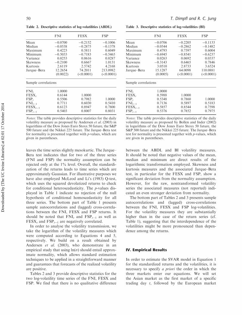
In order to analyse the volatility transmission, wetake the logarithm of the volatility measures whichwere computed according to Equations 4 and 5,respectively. We build on a result obtained byAndersen et al. (2003), who demonstrate in anempirical study that using ln(�) should entail approx-imate normality, which allows standard estimationtechniques to be applied in a straightforward mannerand guarantees that forecasts of the realized volatilityare positive.

Tables 2 and 3 provide descriptive statistics for thetwo log-volatility time series of the FNI, FESX andFSP. We find that there is no qualitative difference

between the ABDL and BI volatility measures.It should be noted that negative values of the mean,median and minimum are direct results of thelogarithmic transformation employed. Skewness andkurtosis measures and the associated Jarque–Beratest, in particular for the FESX and FSP, show asignificant deviation from the normality assumption.However, for the raw, nontransformed volatilityseries the associated measures (not reported) indi-cated an even stronger deviation from normality.

The bottom part of Tables 2 and 3 presents sampleautocorrelations and (lagged) cross-correlationsbetween the FNI, FESX and FSP log-volatilities.For the volatility measures they are substantiallyhigher than in the case of the return series (cf.Table 1), suggesting that the interdependence of thevolatilities might be more pronounced than depen-dence among the returns.

IV. Empirical Results

In order to estimate the SVAR model in Equation 1for the standardized returns and the volatilities, it isnecessary to specify a priori the order in which thethree markets enter our equations. We will setthe Asian market as the first market of a specifictrading day t, followed by the European market

Table 2. Descriptive statistics of log-volatilities (ABDL)

FNI FESX FSP

Mean �0.0700 �0.2152 �0.1006Median �0.0538 �0.2875 �0.1378Maximum 0.4223 0.5811 0.6049Minimum �0.5033 �0.7183 �0.5465Variance 0.0253 0.0616 0.0287Skewness �0.2100 0.6667 1.0131Kurtosis 2.6119 2.5742 4.2168Jarque–Bera 12.2654 74.2011 213.0982

(0.0022) (50.0001) (50.0001)

Sample correlations

FNIt 1.0000FESXt 0.6144 1.0000FSPt 0.5506 0.7982 1.0000FNIt�1 0.7711 0.6030 0.5410FESXt�1 0.6123 0.8947 0.7800FSPt�1 0.5403 0.8007 0.8031

Notes: The table provides descriptive statistics for the dailyvolatility measure as proposed by Andersen et al. (2003) inlogarithms of the Dow Jones Euro Stoxx 50 future, the S&P500 future and the Nikkei 225 future. The Jarque–Bera testfor normality is presented together with p-values, which aregiven in parentheses.

Table 3. Descriptive statistics of log-volatilities (BI)

FNI FESX FSP

Mean �0.0706 �0.2205 �0.1133Median �0.0544 �0.2862 �0.1482Maximum 0.4793 0.7597 0.6004Minimum �0.6945 �0.8541 �0.6237Variance 0.0263 0.0692 0.0337Skewness �0.3143 0.6465 0.7846Kurtosis 3.0510 2.8733 3.6524Jarque–Bera 15.1287 64.0098 110.0881

(0.0005) (50.0001) (50.0001)

Sample correlations

FNIt 1.0000FESXt 0.5988 1.0000FSPt 0.5348 0.7860 1.0000FNIt�1 0.7136 0.5897 0.5183FESXt�1 0.5857 0.8544 0.7598FSPt�1 0.5376 0.7852 0.7975

Notes: The table provides descriptive statistics of the dailyvolatility measure as proposed by Bollen and Inder (2002)in logarithms of the Dow Jones Euro Stoxx 50 future, theS&P 500 future and the Nikkei 225 future. The Jarque–Beratest for normality is presented together with p-values, whichare given in parentheses.

50 T. Dimpfl and R. C. Jung

Dow

nloa

ded

by [

The

UC

Irv

ine

Lib

rari

es]

at 0

2:01

17

Oct

ober

201

4

and the US market, such that in our genericnotation xt¼ (xFNI,t xFESX,t xFSP,t)

0. Alternativeorderings are possible by setting either Eurex or theCME as the first market on trading day t. Theestimation results obtained from these differentmodels are qualitatively similar. Subsequently, wetherefore report only the results obtained with thespecification where the SGX is ordered first. As acheck for robustness of the empirical results pre-sented below, we additionally split the sample butfound no qualitatively different results.

Modelling daily returns

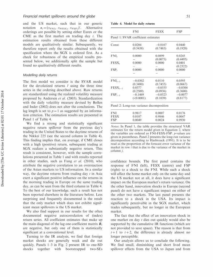
The first model we consider is the SVAR modelfor the devolatized returns ~r using the three timeseries in the ordering described above. Raw returnsare standardized using the realized volatility measureproposed by Andersen et al. (2003). Standardizationwith the daily volatility measure devised by Bollenand Inder (2002) does not alter the conclusions. Thelag length is set to p¼ 1 as suggested by an informa-tion criterion. The estimation results are presented inPanel 1 of Table 4.

We find a strong and statistically significantnegative return spillover from the previous day’strading in the United States to the daytime returns ofthe Nikkei 225 (see the second column in Table 4).This finding implies that, on average, if CME closeswith a high (positive) return, subsequent trading atSGX realizes a substantially negative return. Thisresult is consistent, however, with the sample corre-lations presented in Table 1 and with results reportedin other studies, such as Fung et al. (2010), whoattribute the negative correlation to an overreactionof the Asian markets to US information. In a similarway, the daytime returns from trading day t in Asiaexert a significant positive influence on the returns inthe morning trading in Europe on the same tradingday, as can be seen from the third column in Table 4.To the best of our knowledge, such a result has notbeen reported elsewhere in the literature before. Lesssurprising and frequently documented is the resultthat the only market which does not exhibit signif-icant mean spillovers is the US market.

We also find support in our results for the oftendocumented negative autocorrelation of (index)return series. All coefficient estimates that make upthe main diagonal of the lag one coefficient matrix B1

are negative, but only one of them is statisticallysignificant at a conventional level.

Turning to the IR analysis, we find that foreignmarket shocks are generally weak and die outquickly. Panels 1–3 in Fig. 2 present IR to one-SDshocks together with bootstrapped two-SEs

confidence bounds. The first panel contains theresponse of FNI (left), FESX (centre) and FSP(right) to a shock to the FNI. While such a shockwill affect the home market only on the same day andthe US market not at all, it does have a significantimpact on the European market’s return variance. Onthe other hand, innovation shocks in Europe (secondpanel) do not have a significant impact on either ofthe other two markets. The last panel presents thereaction to a shock in the USA. Its impact issignificantly perceivable in the SGX market, whichtrades subsequently, but no longer in the Europeanmarket.

The fact that the effect of an innovation shock inone market on day t dies out quickly would also besupported by the cumulative IR functions (which arenot provided to save space). The reason is that fromtþ 1 to tþ 2, the difference is already almost nolonger perceptible.

Our analysis allows us to conclude the following.We find small, diminishing and short lived meanspillover effects from the USA to Japan and from

Table 4. Model for daily returns

FNI FESX FSP

Panel 1: SVAR coefficient estimates

Const 0.0204 �0.0107 0.0440(0.5438) (0.7483) (0.1920)

FNIt 0.0000 0.0899 0.0245� (0.0073) (0.4495)

FESXt 0.0000 0.0000 0.0401� � (0.2322)

FSPt 0.0000 0.0000 0.0000� � �

FNIt�1 �0.0302 0.0110 0.0595(0.3480) (0.7455) (0.0667)

FESXt�1 0.0377 �0.0555 �0.0304(0.2509) (0.0936) (0.3600)

FSPt�1 �0.1469 �0.0523 �0.0077(50.0001) (0.1039) (0.8177)

Panel 2: Long-run variance decomposition

FNI 0.9817 0.0007 0.0176FESX 0.0107 0.9846 0.0047FSP 0.0049 0.0024 0.9930

Notes: In Panel 1, the table provides the structural VARestimates for the return model given in Equation 2, wherethe variables are ordered as FNI-FESX-FSP. p-values aregiven in parentheses. Panel 2 presents the long-run variancedecomposition according to Hasbrouck (1991). It is to beread as the proportion of the forecast error variance of themarket in row i that is due to the variance of the market incolumn j.

Financial market spillovers around the globe 51

Dow

nloa

ded

by [

The

UC

Irv

ine

Lib

rari

es]

at 0

2:01

17

Oct

ober

201

4

Japan to Europe, following the chronological order-ing as expected. Moreover, the US market turns outto be robust against return spillovers. A possibleexplanation may be the differing speed of informationprocessing in the USA compared to Japan andEurope, which is compatible with the theoreticalmodels discussed in the introduction.

Volatility modelling

The second model we examine is the SVAR model forthe two different volatility measures � (see Equations4 and 5), once again using the ordering as set outabove. In order to capture the possible long memory

property of the log realized volatility time series,Andersen et al. (2007) suggest to resort to the HAR-RV class of volatility models suggested by Corsi(2009). We find that the long persistence in our data isdescribed best by a model which includes daily,weekly and half-yearly lags. We therefore specify aVector Autoregression (VAR) which includes lagsp¼ (1, 5, 120). The results presented in the followingare not altered if the half-yearly lag is, for example,specified as lag 125 or 130. It also turns out that theestimation results based on the ABDL and the BIvolatility measures are not qualitatively different. Weconclude from this finding that both measuresefficiently account for possible microstructure effects

Fig. 2. Return model: impulse response

Notes: The graphs depict the response of the FNI (left column), FESX (middle column), and FSP returns (right column) to aone SD shock in Singapore (first row), Europe (second row), and the USA (third row), respectively. The dashed lines are twoSE bounds.

52 T. Dimpfl and R. C. Jung

Dow

nloa

ded

by [

The

UC

Irv

ine

Lib

rari

es]

at 0

2:01

17

Oct

ober

201

4

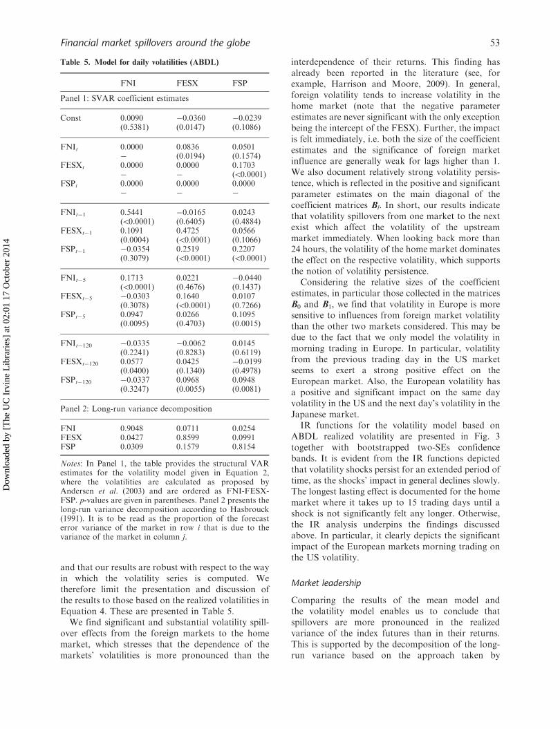
and that our results are robust with respect to the wayin which the volatility series is computed. Wetherefore limit the presentation and discussion ofthe results to those based on the realized volatilities inEquation 4. These are presented in Table 5.

We find significant and substantial volatility spill-over effects from the foreign markets to the homemarket, which stresses that the dependence of themarkets’ volatilities is more pronounced than the

interdependence of their returns. This finding hasalready been reported in the literature (see, forexample, Harrison and Moore, 2009). In general,foreign volatility tends to increase volatility in thehome market (note that the negative parameterestimates are never significant with the only exceptionbeing the intercept of the FESX). Further, the impactis felt immediately, i.e. both the size of the coefficientestimates and the significance of foreign marketinfluence are generally weak for lags higher than 1.We also document relatively strong volatility persis-tence, which is reflected in the positive and significantparameter estimates on the main diagonal of thecoefficient matrices Bl. In short, our results indicatethat volatility spillovers from one market to the nextexist which affect the volatility of the upstreammarket immediately. When looking back more than24 hours, the volatility of the home market dominatesthe effect on the respective volatility, which supportsthe notion of volatility persistence.

Considering the relative sizes of the coefficientestimates, in particular those collected in the matricesB0 and B1, we find that volatility in Europe is moresensitive to influences from foreign market volatilitythan the other two markets considered. This may bedue to the fact that we only model the volatility inmorning trading in Europe. In particular, volatilityfrom the previous trading day in the US marketseems to exert a strong positive effect on theEuropean market. Also, the European volatility hasa positive and significant impact on the same dayvolatility in the US and the next day’s volatility in theJapanese market.

IR functions for the volatility model based onABDL realized volatility are presented in Fig. 3together with bootstrapped two-SEs confidencebands. It is evident from the IR functions depictedthat volatility shocks persist for an extended period oftime, as the shocks’ impact in general declines slowly.The longest lasting effect is documented for the homemarket where it takes up to 15 trading days until ashock is not significantly felt any longer. Otherwise,the IR analysis underpins the findings discussedabove. In particular, it clearly depicts the significantimpact of the European markets morning trading onthe US volatility.

Market leadership

Comparing the results of the mean model andthe volatility model enables us to conclude thatspillovers are more pronounced in the realizedvariance of the index futures than in their returns.This is supported by the decomposition of the long-run variance based on the approach taken by

Table 5. Model for daily volatilities (ABDL)

FNI FESX FSP

Panel 1: SVAR coefficient estimates

Const 0.0090 �0.0360 �0.0239(0.5381) (0.0147) (0.1086)

FNIt 0.0000 0.0836 0.0501� (0.0194) (0.1574)

FESXt 0.0000 0.0000 0.1703� � (50.0001)

FSPt 0.0000 0.0000 0.0000� � �

FNIt�1 0.5441 �0.0165 0.0243(50.0001) (0.6405) (0.4884)

FESXt�1 0.1091 0.4725 0.0566(0.0004) (50.0001) (0.1066)

FSPt�1 �0.0354 0.2519 0.2207(0.3079) (50.0001) (50.0001)

FNIt�5 0.1713 0.0221 �0.0440(50.0001) (0.4676) (0.1437)

FESXt�5 �0.0303 0.1640 0.0107(0.3078) (50.0001) (0.7266)

FSPt�5 0.0947 0.0266 0.1095(0.0095) (0.4703) (0.0015)

FNIt�120 �0.0335 �0.0062 0.0145(0.2241) (0.8283) (0.6119)

FESXt�120 0.0577 0.0425 �0.0199(0.0400) (0.1340) (0.4978)

FSPt�120 �0.0337 0.0968 0.0948(0.3247) (0.0055) (0.0081)

Panel 2: Long-run variance decomposition

FNI 0.9048 0.0711 0.0254FESX 0.0427 0.8599 0.0991FSP 0.0309 0.1579 0.8154

Notes: In Panel 1, the table provides the structural VARestimates for the volatility model given in Equation 2,where the volatilities are calculated as proposed byAndersen et al. (2003) and are ordered as FNI-FESX-FSP. p-values are given in parentheses. Panel 2 presents thelong-run variance decomposition according to Hasbrouck(1991). It is to be read as the proportion of the forecasterror variance of the market in row i that is due to thevariance of the market in column j.

Financial market spillovers around the globe 53

Dow

nloa

ded

by [

The

UC

Irv

ine

Lib

rari

es]

at 0

2:01

17

Oct

ober

201

4

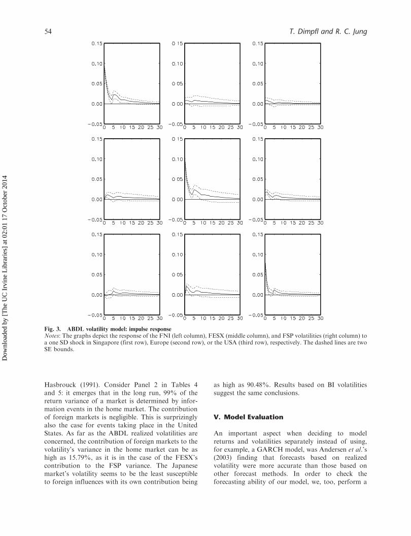
Hasbrouck (1991). Consider Panel 2 in Tables 4and 5: it emerges that in the long run, 99% of thereturn variance of a market is determined by infor-mation events in the home market. The contributionof foreign markets is negligible. This is surprizinglyalso the case for events taking place in the UnitedStates. As far as the ABDL realized volatilities areconcerned, the contribution of foreign markets to thevolatility’s variance in the home market can be ashigh as 15.79%, as it is in the case of the FESX’scontribution to the FSP variance. The Japanesemarket’s volatility seems to be the least susceptibleto foreign influences with its own contribution being

as high as 90.48%. Results based on BI volatilitiessuggest the same conclusions.

V. Model Evaluation

An important aspect when deciding to modelreturns and volatilities separately instead of using,for example, a GARCH model, was Andersen et al.’s(2003) finding that forecasts based on realizedvolatility were more accurate than those based onother forecast methods. In order to check theforecasting ability of our model, we, too, perform a

Fig. 3. ABDL volatility model: impulse responseNotes: The graphs depict the response of the FNI (left column), FESX (middle column), and FSP volatilities (right column) toa one SD shock in Singapore (first row), Europe (second row), or the USA (third row), respectively. The dashed lines are twoSE bounds.

54 T. Dimpfl and R. C. Jung

Dow

nloa

ded

by [

The

UC

Irv

ine

Lib

rari

es]

at 0

2:01

17

Oct

ober

201

4

simple forecast evaluation. We evaluate whether

an out-of-sample return forecast based on the

estimated SVAR models can compete with a univar-

iate modelling approach forecasting the devolatized

return and the realized volatility separately, and

compare these two forecasts to a univariate

GARCH(1,1)-model-based forecast, as well as a

forecast based on a univariate Autoregressive AR(1)

model. Note that the evaluation is intended to

compare a forecast of the log-returns, not the

devolatized returns. We therefore undo the devolati-

zation when using the multivariate and univariate

models, i.e. we forecast the volatility and the

standardized returns separately and combine the

results according to Equation 3. In order to account

for distributional aspects of the log-returns, both the

GARCH model and the univariate AR(1) model are

estimated by maximum likelihood assuming t-dis-

tributed errors.

To evaluate the accuracy of the forecast we use the

Mean Absolute Error (MAE), the Mean Absolute

Percent Error (MAPE) and the Mean Percent Error

(MPE) measures (e.g. Makridakis et al., 1998) which

are defined as

MAE ¼1

s

Xst¼1

rt � r?t�� �� � 100

MAPE ¼1

s

Xst¼1

rt � r?trt

�������� � 100

MPE ¼1

s

Xst¼1

rt � r?trt� 100

where s is the forecast horizon and r?t is the forecast

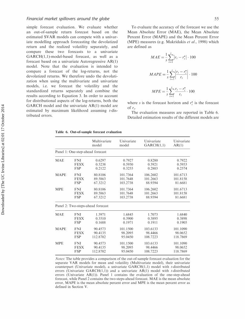
of rt.The evaluation measures are reported in Table 6.

Detailed estimation results of the different models are

Table 6. Out-of-sample forecast evaluation

Multivariate Univariate Univariate Univariatemodel model GARCH(1,1) AR(1)

Panel 1: One-step-ahead forecast

MAE FNI 0.6297 0.7927 0.8280 0.7922FESX 0.5238 0.5950 0.5921 0.5953FSP 0.2122 0.3255 0.2803 0.2574

MAPE FNI 80.8106 101.7364 106.2602 101.6713FESX 89.5863 101.7648 101.2663 101.8158FSP 67.3212 103.2738 88.9394 81.6681

MPE FNI 80.8106 101.7364 106.2602 101.6713FESX 89.5863 101.7648 101.2663 101.8158FSP 67.3212 103.2738 88.9394 81.6681

Panel 2: Two-steps-ahead forecast

MAE FNI 1.5971 1.6845 1.7073 1.6840FESX 0.3510 0.3900 0.3895 0.3898FSP 0.1688 0.1971 0.1911 0.1905

MAPE FNI 90.4573 101.1500 103.6133 101.1090FESX 90.4135 98.2095 98.4466 98.0652FSP 112.8702 95.0450 108.7223 118.7869

MPE FNI 90.4573 101.1500 103.6133 101.1090FESX 90.4135 98.2095 98.4466 98.0652FSP 112.8702 95.0450 108.7223 118.7869

Notes: The table provides a comparison of the out-of-sample forecast evaluation for theseparate VAR models for mean and volatility (Multivariate model), their univariatecounterpart (Univariate model), a univariate GARCH(1,1) model with t-distributederrors (Univariate GARCH(1,1)) and a univariate AR(1) model with t-distributederrors (Univariate AR(1)). Panel 1 contains the evaluation of the one-step-aheadforecast, while Panel 2 contains the two-steps-ahead forecast. MAE is the mean absoluteerror, MAPE is the mean absolute percent error and MPE is the mean percent error asdefined in Section V.

Financial market spillovers around the globe 55

Dow

nloa

ded

by [

The

UC

Irv

ine

Lib

rari

es]

at 0

2:01

17

Oct

ober

201

4

not reported, but are available from the authors uponrequest. We find that the multivariate model alwaysperforms better than any of the univariate models,with the only exception of the FSP two-step-aheadforecast. To justify the using of our estimationprocedure in preference to the GARCH or ARapproaches, consider the differences between thesemodels in the MAPE of the one-step-ahead forecast.When modelling mean and volatility separately, theforecast of the FNI based on this approach is betterby almost 5 percentage points than the forecast basedon the GARCH model, and still slightly better thanthe forecast based on the AR(1)-model. In the case ofthe FESX forecast, the model is only slightly worse(by 0.5 percentage points) than the GARCH modeland performs slightly better than the AR(1)-model. Inthe case of the FSP, the univariate model performsworse than the GARCH or AR model. However, inthe two-step-ahead forecast this is reversed, and itperforms decisively better. Forecasts errors of theFNI and FESX remain approximately stable in thetwo-step-ahead forecast.

To summarize the findings of the forecast evalua-tion, we can state that there are clearly two advan-tages in our modelling approach. First, the forecastbased on the strategy of modelling returns andvariances separately pays off in terms of forecastaccuracy, in particular when it comes to longerhorizon forecasts. Second, by taking this approachwe avoid the delicate issues that arise when using amultivariate GARCH model within the context of astructural VAR approach, especially the issues con-cerning the identification of a structural GARCHprocess.

VI. Concluding Remarks

Our article contributes to the fast-growing body ofliterature in empirical financial economics dedicatedto the investigation of international financial marketlinkages. We propose a new modelling strategydesigned to capture the short-run daytime spilloverdynamics of the main financial centres around theglobe. Specifically, we employ SVAR models for themean and the volatilities of the daytime returns,which draw their structure from the natural chrono-logical ordering of the trading in the three marketsused in our study (Europe, USA and Japan). Thisallows us to provide IR and variance decompositionanalysis, as well as Granger-type causality testing,within this well-established framework.

For the mean system, we find only short-livedsignificant spillovers from the USA to Japan and

from Japan to Europe, albeit in a small order ofmagnitude. It emerges that the Japanese market’sreturns are the most susceptible to foreign informa-tion, originating essentially from the United States.The European market, on the other hand, reacts onlyto information spilling over from the Japanesemarket. This indicates that, while the US andEuropean markets are closed, the markets in Asiaefficiently process information which then spill overto Europe, the market which opens first after Asianmarkets close. The US market, however, seems tohave a particular position in that we do notfind spillovers either from Europe or from Japan tothe USA.

As regards volatility spillovers, we find that allmarkets react more intensely to the volatility of theprevious market than in the case of the returnspillovers. The effect originating in foreign marketsdies out within 2–3 trading days; the influence of thehome market is persistent, however, for approxi-mately 10 days. In contrast to the findings for themean model, the timing seems to be less important forvolatility spillovers as it is not always the marketwhich was open directly before that exerts thegreatest influence. Our findings are robust withrespect to the way the volatility series is computed.

The dynamical systems estimated here can ulti-mately be employed to trace and forecast the impact ofa shock in one of the world’s leading markets on theother markets, as well as to generate a forecast of thereturns in the markets. We find that the contributionof the separate modelling approach in the multivariatecontext is threefold. First, the multivariate structureallows for a more accurate forecast of the return seriesthan a univariate approach. Second, the (univariate)separation of returns and volatilities and theirdetached forecast turns out to perform, on average,better than a univariate forecast based on a GARCHmodel or an ARmodel. And finally, the application ofstructural VARs is econometrically easier to managethan using multivariate GARCH models within thisstructural context. All in all, the model seems able totrace the linkages between international stock mar-kets, and highlights once again the interdependence ofglobal financial markets.

References

Admati, A. R. and Pfleiderer, P. (1988) A theory ofintraday patterns: volume and price variability, TheReview of Financial Studies, 1, 3–40.

Andersen, T. G., Bollerslev, T., Christoffersen, P. F. andDiebold, F. X. (2006) Practical volatility and correla-tion modeling for financial market risk management,

56 T. Dimpfl and R. C. Jung

Dow

nloa

ded

by [

The

UC

Irv

ine

Lib

rari

es]

at 0

2:01

17

Oct

ober

201

4

in The Risks of Financial Institutions, Chap. 17 (Eds)M. Carey and R. M. Stulz, University of ChicagoPress, Chicago, Illinois, pp. 513–48.

Andersen, T. G., Bollerslev, T. and Diebold, F. X. (2007)Roughing it up: including jump components in themeasurement, modeling, and forecasting of returnvolatility, The Review of Economics and Statistics, 89,701–20.

Andersen, T. G., Bollerslev, T. and Diebold, F. X. (2010)Parametric and nonparametric volatility measurement,in Handbook of Financial Econometrics (Eds)Y. Aıt-Sahalia and L. P. Hansen, Elsevier ScienceLtd, Amsterdam, pp. 67–138.

Andersen, T. G., Bollerslev, T., Diebold, F. X. andLabys, P. (2003) Modeling and forecasting realizedvolatility, Econometrica, 71, 529–626.

Baur, D. and Jung, R. C. (2006) Return and volatilitylinkages between the US and the German stockmarket, Journal of International Money and Finance,25, 598–613.

Bollen, B. and Inder, B. (2002) Estimating daily volatility infinancial markets utilizing intraday data, Journal ofEmpirical Finance, 9, 551–62.

Corsi, F. (2009) A simple approximate long-memory modelof realized volatility, Journal of FinancialEconometrics, 7, 174–96.

Diebold, F. X. and Yilmaz, K. (2009) Measuring financialasset return and volatility spillovers, with applicationto global equity markets, The Economic Journal, 119,158–71.

Fung, A. K. W., Lam, K. and Lam, K. M. (2010) Do theprices of stock index futures in Asia overreact to USmarket returns?, Journal of Empirical Finance, 17,428–40.

Gallo, G. M. and Otranto, E. (2008) Volatility spillovers,interdependence and comovements: a Markov switch-ing approach, Computational Statistics and DataAnalysis, 52, 3011–26.

Ge�bka, B. and Serwa, D. (2007) Intra- and inter-regionalspillovers between emerging capital markets aroundthe world, Research in International Business andFinance, 21, 203–21.

Hamao,Y.,Masulis, R.W. andNg,V. (1990)Correlations inprice changes and volatility across international stockmarkets, The Review of Financial Studies, 3, 281–307.

Harrison, B. and Moore, W. (2009) Spillover effects fromLondon and Frankfurt to Central and Eastern

European stock markets, Applied FinancialEconomics, 19, 1509–21.

Hasbrouck, J. (1991) The summary informativeness ofstock trades: an econometric analysis, The Review ofFinancial Studies, 4, 571–95.

Kyle, A. S. (1985) Continuous auctions and insider trading,Econometrica, 53, 1315–35.

Lin, W. L., Engle, R. F. and Ito, T. (1994) Do bulls andbears move across borders? International transmissionof stock returns and volatility, The Review of FinancialStudies, 7, 507–38.

Makridakis, S., Wheelwright, S. C. and Hyndman, R. J.(1998) Forecasting – Methods and Applications,3rd edn, John Wiley & Sons, Inc., New York.

McLeod, A. I. and Li, W. K. (1983) Diagnostic checkingARMA time series models using squared-residualautocorrelations, Journal of Time Series Analysis, 4,269–73.

Melvin, M. and Peiers Melvin, B. (2003) The globaltransmission of volatility in the foreign exchangemarket, Review of Economics and Statistics, 85, 670–9.

Menkveld, A. J., Koopman, S. J. and Lucas, A. (2007)Modeling around-the-clock price discovery forcross-listed stocks using state space methods,Journal of Business and Economic Statistics, 25,213–25.

Pesaran, B. and Pesaran, M. H. (2010) Conditionalvolatility and correlations of weekly returns and theVAR analysis of 2008 stock market crash, EconomicModelling, 27, 1398–416.

Pritsker, M. (2001) The channels for financial contagion,in International Financial Contagion, Chap. 4 (Eds)S. Claessens and K. J. Forbes, Springer-Verlag, Berlin,pp. 67–95.

Ryoo, H. J. and Smith, G. (2004) The impact of stock indexfutures on the Korean stock market, Applied FinancialEconomics, 14, 243–51.

Savva, C. S., Osborn, D. R. and Gill, L. (2009) Spilloversand correlations between US and major Europeanstock markets: the role of the euro, Applied FinancialEconomics, 19, 1595–604.

Soriano, P. and Climent, F. J. (2006) Volatility transmis-sion models: a survey, Revista de Economıa Financiera,10, 32–81.

Susmel, R. and Engle, R. F. (1994) Hourlyvolatility spillovers between international equitymarkets, Journal of International Money and Finance,13, 3–25.

Financial market spillovers around the globe 57

Dow

nloa

ded

by [

The

UC

Irv

ine

Lib

rari

es]

at 0

2:01

17

Oct

ober

201

4