Embed Size (px)
Citation preview

FIELD ORIENTED CONTROL OF STEP MOTORS
BHAVINKUMAR SHAH
Bachelor of Engineering in Electrical Engineering
SVMIT - Bharuch, India
June, 2000
Submitted in partial fulfillment of requirements for the degree
MASTER OF SCIENCE IN ELECTRICAL ENGINEERING
at the
CLEVELAND STATE UNIVERSITY
December, 2004
This thesis has been approved
for the Department of Electrical and Computer Engineering
and the College of Graduates Studies by
_________________________________________________ Thesis Committee Chairperson, Dr. Dan Simon
_____________________________ Department/Date
_________________________________________________ Thesis Committee Member, Dr. Zhiqiang Gao
_____________________________ Department/Date
_________________________________________________ Thesis Committee Member, Dr. Ana Stankovic
_____________________________ Department/Date

To
My parents: Satish Shah & Sharmistha Shah
My Brother: Hardik Shah

ACKNOWLEDGEMENT
I would like to express my sincere gratitude to my advisor Dr. Dan Simon, for his
guidance, encouragement and invaluable help throughout the course of my study and
thesis.
I would like to thank my committee members Dr. Zhiqiang Gao and Dr. Ana
Stankovic for their support and time in evaluating my thesis.
I would like to thank Dennis Feucht of Innovatia Laboratories for his technical
assistance.
I would also like to thank my friends at the Embedded Control Systems Research
Laboratory for offering me encouragement and advice whenever I needed.
A special thanks to my family for their continuous encouragement and support.

FIELD ORIENTED CONTROL OF STEP MOTORS
BHAVINKUMAR SHAH
ABSTRACT
Despite recent performance improvements in step motor modeling and control
algorithms, open-loop control still falls significantly short of achieving maximum motor
performance. Step motors, which are often used in industrial applications, can exhibit
stepping resonance and skipped steps. Field oriented control can eliminate resonance
anomalies and skipped steps. The maximum theoretical performance from the step motor
can be derived by driving a step motor with field oriented control rather than stepping.
In field oriented control, the motor input currents are adjusted to set a specific angle
between the stator magnetic field and rotor magnetic field. From basic motor theory,
when the stator magnetic field vector is maintained at a phase angle of 900 ahead of the
rotor magnetic field, maximum torque is produced. The torque varies with the sine of this
torque angle between the stator and rotor magnetic field vectors. By sensing rotor
position, the phase of the rotor magnetic field can be determined and the current
excitation kept 900 ahead of it. At this optimal torque angle, maximum torque is available
(for given power supply voltage) under steady-state and transient operation. This
approach is not widespread because electronic components historically have constrained
drives to simple schemes such as stepping, and the full dynamic theory of electric
machines was not worked out until the 1980’s. The resulting performance advantages of
field oriented control over stepping compensate for the additional circuit cost and
complexity.

TABLE OF CONTENTS
LIST OF FIGURES ................................................................................................................X
LIST OF TABLES ..............................................................................................................XII
CHAPTER
I. DIGITAL SIGNAL PROCESSING AND STEP MOTOR CONTROL...…….1
1.1 Analog Control Systems..........................................................................…...2
1.2 DSP Based Digital Control Systems........................................................…...3
1.3 Step Motor System………………………...………………...………………4
1.3.1 Controller......................................................................…..........5
1.3.2 Driver……………………………………………......................5
1.3.3 Step Motor………………………….………………….............5
1.4 SMC3 Background…………………..………………………………...........6
1.5 Thesis Organization ….………………………..………………………........6
II. STEP MOTORS........……………………………………….……………………….8
2.1 Types of Step Motors…….....………...……………………………………..9
2.1.1 Variable Reluctance Motors.......................................................9
2.1.2 Permanent Magnet Step Motors................................................11
2.1.3 Hybrid Step Motors...................................................................12
2.2 Comparison of Motor Types.........................................................................14
2.2.1 Variable Reluctance versus Permanent Magnet or Hybrid.......14
2.2.2 Hybrid versus Permanent Magnet.............................................15

2.3 Step Motor Modes of Excitation...................................................................16
2.3.1 Full Step Operation...................................................................16
2.3.2 Half Step Operation..................................................................17
2.3.3 Micro Step Operation................................................................17
2.4 Types of Drives.............................................................................................18
2.4.1 Unipolar Drives.........................................................................18
2.4.2 Bipolar Drives...........................................................................19
2.5 Torque Production in Hybrid Step Motors...................................................19
2.6 Field Oriented Control..................................................................................23
2.6.1 Sine/Cosine wave generation....................................................25 2.6.2 Frequency Synthesis.................................................................28 2.7 Torque vs Speed Characteristics...................................................................29 2.8 Effect of Inductance on Winding Current.....................................................31 2.9 Longevity......................................................................................................33 2.10 Resonance.....................................................................................................35 2.10.1 Low-Frequency Resonance.......................................................35
2.10.2 Medium-Range Instability........................................................35
2.10.3 Higher-Range Oscillation.........................................................36
III. THE HARDWARE DESIGN OF THE SMC3…………….........………………37
3.1 SMC3 Design Overview...............................................................................38 3.2 Dual PWM Generator...................................................................................39 3.3 Power Driver Circuit.....................................................................................43 3.3.1 PWM Switching Technique......................................................46

3.3.2 Maximum Current Limiter........................................................47 3.4 Sensing Circuit..............................................................................................48 3.4.1 Zero-Crossing Detection...........................................................48 3.4.2 Position Sensor.........................................................................49
3.4.3 Current Sensing.........................................................................50
3.5 Speed Input...................................................................................................53
3.5.1 AD7811 A/D Converter............................................................54
3.5.2 Reference Voltage.....................................................................54
3.5.3 External latch............................................................................55
3.6 ADSP-2101..................................................................................................56
3.6.1 Data Transfer............................................................................57
3.6.2 Serial Ports................................................................................58
3.6.3 Interrupts...................................................................................60
3.6.4 System Clock............................................................................61
IV. CURRENT CONTROL IN STEP MOTORS...….…..………...………………64
4.1 Motor Equivalent Circuit...............................................................................65
4.1.1 Motor Transfer Function...........................................................66
4.1.2 Torque Constant........................................................................67
4.1.3 PID Controller...........................................................................69
4.2 SMC3 Open-Loop Simulink Model..............................................................70
4.2.1 SMC3 Closed-Loop Model.......................................................71
4.2.2 PID Controller Tuning..............................................................73
V. SENSORLESS STEP MOTOR CONTROL.................................................…...75

5.1 Kalman Filter.................................................................................................75
5.1.1 Discrete-Time Kalman filter.....................................................77
5.1.2 Extended Kalman Filter (EKF).................................................78
5.2 EKF Implementation for a Step Motor..........................................................80
5.2.1 Continuous Step Motor Model.................................................80
5.2.2 Discretization of the Step Motor Model...................................81
5.2.3 Simulation and Real-Time Implementation..............................82
VI. CONCLUSIONS AND FUTURE RESEARCH.........................................…...86
BIBLIOGRAPHY............................................................................................................88
APPENDIX......................................................................................................................91
A Software Listing…………………………………………...……...………...92

LIST OF FIGURES
Figure Page
1. Step Motor System……………………………………………………..............….4
2. Variable Reluctance Motor……………………….…….…………………………9
3. Permanent Magnet Motor………..………………………………………………11
4. Hybrid Step Motor……………………………………………..………………...12
5. Unipolar Drive………………………..………………………………………….18
6. Bipolar Drive……………………..……………………………………………...19
7. Two Phase Hybrid Step Motor……………..…………………………………....20
8. Speed-Torque Curves………………………………..…………………………...30
9. Winding Model…………………………..………………………………………31
10. Winding Current……………………...………………………………………….32
11. SMC3 ECB (Electronic Circuit board)……………...…………………………...38
12. SMC3 Hardware Functional Diagram…………………………...………………39
13. Dual PWM-generator………………………………………………...…………..42
14. Power Driver and Sensing Circuit……………………...………………………..45
15. Winding Current and Supply Voltage…………………..……………………….47
16. Back emf voltage and zero crossing comparator…………………...……………49
17. Position Sensor………………………...………………………………………...50
18. Current Sensing Circuit………..………………………………………………...51
19. DSP and Speed Input……………………...……………………………………..52
20. Speed Command Interface…...…………………………………………………..53
21. ADSP-2101 System………...……………………………………………………56
22. ADSP-2101 Block Diagram………………...…………………………………...57
23. External Crystal Connection for the ADSP-2101…………...…………………...61
24. Per Phase Equivalent Circuit…………………...………………………………..65
25. Winding Back-emf Voltage………...……………………………………………68
26. SMC3 Open-Loop Model………………………………………………………..70
27. SMC3 Closed-Loop Model………………...…………………………………….71
28. Simulated Winding Current………………...……………………………………72
29. Experimental Winding Current……...…………………………………………...73

LIST OF TABLES
Table Page
1. Look-up Table for Encoder Information................................................................27
2. Potentiometer Input and Corresponding ADC Count……………………………54
3. Interface Signal…………………………………………………………………..59
4. ADSP-2101 Pin Definitions...................................................................................62

1
CHAPTER I
DIGITAL SIGNAL PROCESSING AND STEP MOTOR
CONTROL
Electric motors are everywhere in the modern world. The worldwide market for electric
motors drives will grow from $12.5 billion in 2000 to $19.1 billion in 2005, according to
a market research study by Drives Research Corporation. Electric motors consume two-
thirds of the industrial electric consumption and one fourth of the residential electric
consumption.
Saving energy has become a key concern because of the continuing increase in energy
usage and new government regulation. The new electric drive system must have higher
efficiency and at the same time reduced electromagnetic interference. The new system
must be flexible to incorporate modification with minimum time. All of these
improvements must be achieved while decreasing system cost.
The DSP (digital signal processor) is now emerging as a key technology enabling the
electric drive to be a smoother, more energy-efficient and most importantly cost-effective

2
solution. This is being exploited in a whole spectrum of applications, such as washing
machines, heating and air conditioning, and electric power assist in cars.
A digital signal processor utilizes a high degree of parallelism, optimized for very fast
mathematical calculations. DSPs usually incorporate specialized hardware for the
efficient implementation of digital filters, matrix operations and frequency
transformation. Until recently they have been used predominately in telecommunications
applications which require complex filtering. The computing power of DSPs allows users
to exploit software modeling to implement closed-loop motor control, creating a shift
from hardware to software based systems. The increased power of DSPs can be used in
several ways. The first is simply to run existing algorithms faster and improve the
dynamic response of the system. The second is to use it to implement more complex
closed loop sensorless control algorithms.
1.1 Analog Control Systems
Traditionally electric motor drives are designed with relatively inexpensive analog
components. Analog controls offer the following advantages over digital control systems.
(1) Fast torque and speed control is achieved as data is processed in real time.
(2) Because of high bandwidth, they offer higher resolution over wider bandwidth.
However there are several drawbacks to analog systems.
(1) As motor control systems age, the wear and tear on mechanical components may
result in a loss of control, since the control system is tuned to the characteristics
of the system when it was new. Temperature also can cause component variation.
So the analog system requires regular adjustment.

3
(2) In order to control parameters, analog systems require expensive sensors and
more physical parts than digital systems, which reduces the reliability of the
system.
(3) Upgrades are difficult because the design is hardwired.
1.2 DSP Based Digital Control Systems
The DSP based digital control system offers the following advantages over analog
systems.
(1) The enhanced math capabilities of a DSP result in the implementation of real-time
filter structures that can extract or recreate required feedback signals that would
otherwise require expensive sensors to detect. This provides an immediate size
and cost advantage.
(2) It reduces acoustic noise from the motor when running at lower speed. This opens
up many new applications where step motors have previously been excluded due
to motor noise. Low-noise motor operation is achieved because the PWM
switching pulses applied to the motor drivers are generated by the processor, and
can be precisely controlled in width and frequency so that they are inaudible at
standstill.
(3) The implementation of self-tuning regulators or model reference adaptive controls
on a DSP can often extend the life of the system, making it more reliable over a
wider range of parameters.
(4) The upgrades are easily made in software, so the system is more robust.

4
(5) Efficient control using DSPs make it possible to reduce torque ripple and
harmonics. DSP based systems improve dynamic behavior over a wider speed
range. The motor design can be optimized due to lower vibrations and lower
power losses such as harmonic losses in the rotor. Smooth operation with higher
efficiency is achieved.
(6) A single-chip control system is possible as the encoder interface, PWM
generators, multiple synchronous A/Ds , and more, are all available on the same
chip with the DSP.
(7) Real-time generation of smooth, near optimal reference profiles and move
trajectories is possible, which results in better performance.
1.3 Step Motor System
Figure 1. Step Motor System
A typical step motor system is shown in Figure 1. A step motor system consists of
three basic elements: a controller, a driver, and a step motor.

5
1.3.1 Controller
The controller is a DSP or microprocessor which is capable of generating step pulses and
direction signals for the driver. Controlling the speed or torque of a motor accurately
requires the use of a closed loop control strategy which feeds back motor parameters.
These parameters may include rotor position or phase current. The controller implements
complex software algorithms with or without sensors. It is also capable of measuring key
system parameters such as bus voltage and temperature.
1.3.2 Driver
The step motor driver receives low-level signals from the controller and converts them
into pulses to run the motor. There are numerous types of drivers, with different power
ratings and construction topologies. The speed-torque requirements and winding
configuration determines which step motor drive is selected.
1.3.3 Step Motor
The step motor is a synchronous motor which is designed to rotate through a specific
angle for each electrical pulse received from the driver unit. Step motors are low in cost
because of their high volume use in industry. The step motor is a permanent magnet
motor with many poles. They can produce high torque at a given motor winding current.
This makes the step motor ideal for precise motion control. Linear precise positioning
systems are required in a variety of applications including high and low propulsion
technology, computer peripherals, machine tools, and robotics.

6
Step motor can be run in open-loop or closed-loop mode. In closed-loop mode, the
motor is used like a conventional servo motor. A signal from the output feedback is used
to operate a gate controlling the pulses from a pulse generator.
1.4 SMC3 Background
The SMC3 (Step Motor Controller-3) drive is designed by Dennis Feucht of Innovatia
Laboratories. It is design to run two phase step motors and it is advanced version of
SMC1 and SMC2. The SMC1 uses low-cost components in a semi-discrete
implementation, which provides greater circuit observability during design development.
It is adaptable to a wide range of power amplifiers. The SMC2 is a semi-discrete
implementation of a sensor based, field-oriented control of a step motor. The SMC1 and
SMC2 use a microcontroller while the SMC3 uses a DSP (ADSP-2101). The DSP allows
complex functions to be implemented with the flexibility of software, rather than custom
hardware which is function and application specific. So SMC3 uses less physical
components compared to SMC1 and SMC2. The SMC1 and SMC2 control the current
using a hardware approach (chopper control) while the SMC3 controls the current using
control firmware (PID control). The main research of this thesis was to debug and
troubleshoot hardware and implement current control for the SMC3 for sensorless step
motor control.
1.5 Thesis Organization
The present research work focuses on the implementation of current control for field-
oriented controlled step motor so that sensorless control can be implemented.

7
Chapter II presents various step motor designs, their operation, advantages, drive
topology, and field-orientation control technique.
Chapter III gives an overview of the SMC3 design and explains about dual PWM
generator, power driver, sensing circuit and DSP.
Chapter IV establishes the need for current control and presents the SMC3 closed loop
model for simulation and compares simulation results with experimental results.
Chapter V provides an overview of sensorless implementation using an extended Kalman
filter for a field-oriented step motor.

8
CHAPTER II
STEP MOTORS
The step motor, also called a stepper motor, is an electromagnetic device that converts
digital pulses into mechanical shaft position. Basically, a step motor is a synchronous
motor with the magnetic field electrically switched to rotate the armature magnet rotor. In
theory a step motor is similar to a permanent magnet synchronous motor. The motor
rotation not only has a direct relation to the number of input pulses, but its speed is
related to the frequency of the pulses. Due to step motor ease of use, simple controls
needs, and precise control, step motors are commonly used in measurement and control
applications. Sample applications include printers, disk drives, robots, and machine tools.
There are several features common to all step motors that make them ideally suited for
these types of applications. These features are
• Brushless: Step motors are brushless. The commutator and brushes of
conventional motors are some of the most failure-prone components; they create
electrical arcing that is undesirable or dangerous in some environments.

9
• Load Independent: Step motors will turn at a set speed regardless of load as long
as the load does not exceed the torque rating.
• Holding Torque: Between steps, the motor hold its position without clutches or
brakes. Thus a step motor can be precisely controlled so that it rotates a desired
number of steps.
• Response: Step motors provide excellent response to rapid deceleration, stopping
and reversal with the appropriate logic.
This chapter describes various types of step motors, their operation, drive topology, mode
of excitation, field-oriented control, speed-torque characteristics and resonances.
2.1 Types of Step Motors
The step motor can be classified into several types according to machine structure and
principle of operation. There are basically three types of step motors; variable reluctance,
permanent magnet and hybrid.
2.1.1 Variable Reluctance Motors
Figure 2. Variable Reluctance Motor

10
The variable reluctance motor is available in single stack or in multi stack. The stator and
the rotor core are normally made of laminated silicon steel, but solid silicon steel rotors
are also extensively employed. Both the stator and rotor materials must have high
permeability and be capable of allowing high magnetic flux to pass through even if a low
magnetomotive force is applied. In a multi stack motor each stack includes a stator held
in position by the outer casing of the motor and carrying the motor windings. The rotor is
fabricated as a single unit, which is supported at each end of the machine by bearings,
and includes a projecting shaft for the connection of external loads.
The basic variable reluctance step motor with three phases and 12 stator poles is
shown in Figure 2. The stator teeth which are 90 degrees apart from each other belong to
the same phase. The rotor has eight teeth. Both the stator and rotor have a toothed
structure. If phase A is excited magnetic flux will be set up in motor. The rotor will then
be positioned so that the stator poles associated with winding A and any four rotor teeth
are aligned. Thus when the rotor teeth and stator teeth are aligned, the magnetic
reluctance is minimized, and this state is an equilibrium position. If phase A is turned off
and phase B is now turned on, the motor reluctance seen from the DC power supply will
be suddenly increased just after switching takes place. So to minimize the reluctance the
rotor will move 150 in the clockwise direction. This process will continue if we turn off
phase B and turn on phase C. After completing a rotor-tooth-pitch rotation in 24 steps,
the rotor will return to its original position. Reversing the procedure (C to A) would result
in a counterclockwise rotation.

11
2.1.2 Permanent Magnet Step Motors
A step motor using a permanent magnet in the rotor is called a permanent magnet (PM)
motor. The rotor is made of ferrite or rare earth material which is permanently
magnetized. An elementary PM motor is shown in Figure 3, which employs a cylindrical
permanent magnet as the rotor and possesses four poles in its stator. Two overlapping
windings are wound as one winding on poles 1 and 3, and these two windings are
separated from each other at terminals to keep them as independent windings. The same
is true for poles 2 and 4. The terminals marked Ca or Cb denote “common” to be
connected to the positive terminal of the power supply as shown in the switching circuit
(Figure 3). If winding A is excited, pole 1 produces a north pole and pole 3 produces a
south pole. If winding A1 is excited the polarity will be reversed. If the windings are
excited in the sequence A → B → A1 → B1 → - - - - - the rotor will be driven in a
clockwise direction. The step length is 900 in this machine. If the number of stator teeth
and magnetic poles on the rotor are both doubled, a two-phase motor with a step length of
450 will be realized. PM motors have simple construction and low cost that makes it an
ideal choice for non-industrial applications, such as a line printer.
Figure 3. Permanent Magnet Motor

12
2.1.3 Hybrid Step Motors
Another type of step motor having a permanent magnet in its rotor is the hybrid motor.
The term ‘hybrid’ derives from the fact that the motor is operated with the combined
principles of the permanent magnet and variable reluctance motors in order to achieve
small step length and high torque in spite of small motor size. Standard hybrid motors
have 50 rotor teeth and rotate at 1.80 degrees per step. Other hybrid motors are available
in 0.9 and 3.6 degree step lengths. Because they exhibit high static and dynamic torque
and run at very small step lengths, hybrid motors are used in a wide variety of industrial
applications.
Figure 4. Hybrid Step Motor
Figure 4 shows a two phase hybrid step motor with four poles. The windings are placed
on poles on the stator and a permanent magnet is mounted on the rotor. The important
feature of the hybrid motor is its rotor structure. A cylindrical or disk-shaped magnet lies
in the rotor core. Both the stator and rotor end-caps are toothed. The toothed end-caps are
normally made of laminated silicon steel. The stator has only one set of winding-excited

13
poles which interact with two rotor teeth. The coil in pole 1 and pole 3 is connected in
series consisting of phase A, and poles 2 and 4 are for phase B. If stator phase A is
excited the top stator pole acquires a north polarity while the bottom stator pole acquires
a south polarity. As a result the top stator pole attracts the rotor’s south pole while the
bottom stator pole aligns with the rotor’s north pole. If the excitation is shifted from
phase A to phase B such that stator pole 2 becomes a north pole and stator pole 4
becomes a south pole, that would cause the rotor to turn 900 in the clockwise direction.
Again phase A is excited with pole 1 as a south pole and pole 3 as a north pole, causing
the rotor to move 900 in the clockwise direction. If excitation is removed from phase A
and phase B is excited such that pole 2 produces a south pole and pole 4 produces a north
pole, that results in rotor movement of 900 in the clockwise direction. Again shifting
excitation from phase B to phase A with stator pole 1 as a north pole and stator pole 3 as
a south pole causes the rotor to move 900 in the clockwise direction. A complete cycle of
excitation for the hybrid motor consists of four states and produces four steps of rotor
movement. The excitation state is the same before and after these four steps, so the
alignment of stator/rotor teeth occurs under the same stator poles. Therefore the step
length for a hybrid motor is given by
Step length = 900 / Nr (2.1.1)
The motor explained above has one rotor pole pair (Nr), so the step length is 900 in this
case.

14
2.2 Comparison of Motor Types
The system designer is faced with the choice of the specific type of step motor, and the
decision is influenced by the application of the motor. Some of these factors are the
torque requirements of the system, and the complexity of the controller.
2.2.1 Variable Reluctance versus Permanent Magnet or Hybrid Variable reluctance motors (VRMs) benefit from the simplicity of their design. These
motors do not require complex permanent magnet rotors, so they are generally more
robust than permanent magnet motors. Variable reluctance motors have two important
advantages when the load must be moved a considerable distance. First, step lengths are
longer than in the hybrid type so fewer steps are required to move a given distance. A
reduction in the number of steps implies fewer excitation changes. The speed with which
excitation changes limits the time taken to move the required distance. Second, the
variable-reluctance stepping motor has a lower rotor mechanical inertia than hybrid (and
PM) motors, because there is no permanent magnet on its rotor. In many cases the rotor
inertia contributes a significant proportion of the total inertia load on the motor and
reduction in the inertia allows faster acceleration.
Variable reluctance motors do have a drawback. With sinusoidal exciting currents,
permanent magnet and hybrid motors are very quiet. In contrast, variable reluctance
motors are generally noisy, no matter what drive waveform is used. As a result,
permanent magnet or hybrid motors are generally preferred where noise or vibration is an
issue.

15
With appropriate control systems, both permanent magnet and hybrid motors can be
microstepped, allowing positioning to a fraction of a step, and allowing smooth, jerk-free
moves from one step to next. Microstepping is not generally applicable to variable
reluctance motors. These motors are typically run in full-step increments. Complex
current limiting control is required to achieve high speed with variable reluctance motors.
Compared to variable reluctance motors a hybrid motor (and permanent magnet motor
too) requires less excitation because of the PM rotor. If the stator excitation were to be
removed, the rotor will continue to remain locked into the same position as it is prevented
from moving in either direction by torque caused by the permanent magnet excitation.
This feature favors hybrid (and PM) motors in applications where the rotor position must
be preserved during a power failure.
Although PM motors operate at fairly low speed the PM motor has a relatively high
torque characteristic for a small motor size compared with a variable reluctance motor of
the same size.
2.2.2 Hybrid versus Permanent Magnet
In selecting between hybrid and permanent magnet motors, the two primary issues are
cost and resolution. The same drive electronics and wiring options generally apply to
both motor types.
Permanent magnet motors are, without question, some of the least expensive motors
made. They are sometimes described as can-stack motors because the stator is
constructed as a stack of two windings enclosed in metal stampings that resemble tin cans
and are almost as inexpensive to manufacture. In comparison, hybrid and variable

16
reluctance motors are made using stacked laminations with motor windings that are
significantly more difficult to wind.
Hybrid motors have a small step length, which can be a great advantage when high
resolution angular positioning is required. Compared to PM motors, finer step length for
better resolution is easily obtained in hybrid motors by adding additional rotor teeth.
Hybrid motors suffer some of the vibration problems of variable reluctance motors,
but they are not as severe. They generally can step at rates higher than permanent magnet
motors, although very few of them offer useful torque above 5000 steps per second.
2.3 Step Motor Modes of Excitation
One of the most important decisions to make is the step size (mode) of the motor. This
will be determined by the resolution necessary for particular application. The most
common step sizes for PM motors are 7.5 and 3.6 degrees. Hybrid motors typically have
step sizes ranging from 3.6 degrees to 0.9 degrees. Step motor ‘step modes’ include full,
half, and microstep. The type of step mode output of any motor is dependent on the
design of the driver circuit.
2.3.1 Full Step Operation
Full step mode is achieved by energizing both windings while reversing the current
alternately. Essentially one digital input from the driver is equivalent to one step. If two
phases of the hybrid motor are excited, the torque produced by the motor is increased but
the power supply to the motor is also increased. This can be an important consideration in
17
applications where the power available to drive the motor is limited. The SMC3 motor
has a step length of 1.80.
2.3.2 Half Step Operation
In half step mode, one winding is energized and then two windings are energized
alternately, causing the rotor to rotate at half the distance. An essential advantage of a
step motor operation in half step mode is its position resolution is increased by a factor of
two compares to full step mode. If we have a (1.8)0 full step length, a step length of (0.9)0
is achieved in half step mode. Half step mode also reduces the amount of “jumpiness”
inherent in running in full step mode. The half step system needs twice as many clock
pulses as the full step system; the clock frequency is twice as high as with full step mode,
and half step mode produces only about half of the torque of full step mode.
2.3.3 Micro Step Operation
The full step length of a stepping motor can be divided in to smaller increments of rotor
motion - known as “micro step” - by partially exciting several phase windings. Micro
stepping is a relatively new step motor technology that controls the current in the motor
winding. Micro stepping is typically used in applications that require accurate positioning
and a fine resolution over a wide range of speeds. The major disadvantage of the micro
step drive is the cost of implementation due to the need for partial excitation of the motor
windings at different current levels.

18
2.4 Types of Drives
The step motor driver circuit has to change the current and flux direction in the phase
windings. Stepping requires a change of flux direction, independently in each phase. The
direction change is done by changing the current direction, and may be done in two
different ways: using a unipolar or a bipolar drive.
2.4.1 Unipolar Drives
The name unipolar is derived from the fact that current flow is limited to one direction. A
unipolar drive is fairly simply and inexpensive. The unipolar drive principle requires a
winding with a center tap, or two separate windings per phase. Flux direction is reversed
by moving the current from one half of the winding to the other half. This method
requires only two switches per phase. The unipolar drive utilizes only half the available
copper volume of winding and therefore incurs twice the loss of a bipolar drive at the
same output power. The basic control circuit for a unipolar motor is shown in Figure 5.
Figure 5. Unipolar Drive

19
2.4.2 Bipolar Drives
Bipolar drives are by far the most widely used drives for industrial applications. Although
they are typically more expensive to design, they offer high performance and high
efficiency. The word “bipolar” refers to the principle where the current direction in one
winding is changed by shifting the voltage polarity across the winding terminal. To
change polarity a total of four switches are needed, forming an H-bridge. The bipolar
drive method requires one winding per phase. The motor winding is fully energized by
turning on one set (top and bottom) of the switching transistors. The basic control circuit
for a bipolar motor is shown in Figure 6.
Figure 6. Bipolar Drive
2.5 Torque Production in Hybrid Step Motors
Consider a two phase motor having the pole configuration as shown in Figure 7. To
simplify the analysis, the effects of winding resistance, eddy currents, detent torque,
mutual induction, and hysteresis are neglected. Also magnetic circuits in the motor are
assumed to be linear, that is the magnetic flux induced by the stator currents is
independent of the internal magnet and proportional to the applied emf [1].

20
Figure 7. Two Phase Hybrid Step Motor
From the fundamental law of energy conservation
(Electrical power supplied by source) = (Mechanical output power) + (Rate of increase in
magnetic energy) (2.5.1)
This equation can be written as
( )dt
Li21
Li21
d
dtd
TieieBB
2AA
2
BBAA
���
����
� ∗∗��
���
�+∗∗��
���
�
+��
���
� θ=∗+∗ (2.5.2)
where eA=emf induced in the A phase
eB=emf induced in the B phase
iA= current in the A phase
iB=current in the B phase
LA=inductance of the A phase
LB=inductance of the B phase
T=torque developed

21
�= angular displacement
If the magnetic circuits are linear and the mutual inductance between the two phases is
negligible, the torque can be separated into A and B components such that
BA ��T += (2.5.3)
Hence
( ) ( )dt
Lid21
dtd�
�ie AA2
AAA
∗∗��
���
�+��
���
�=∗− (2.5.4)
( ) ( )dt
Lid21
dtd�
�ie BB2
BBB
∗∗��
���
�+��
���
�=∗− (2.5.5)
The terminal voltage for each phase is the sum of two components; the voltage generated
by the permanent-magnet flux linking the phase windings and that caused by current
flowing through the phase inductance. The equation for phase A is therefore rewritten as
( ) ( )dt
Lid21
dtd�
�iee AA2
AALAgA
∗∗��
���
�+��
���
�=∗+− (2.5.6)
where gAe is the voltage generated by the permanent-magnet flux linking with phase A
and LAe is the voltage induced by the current in phase A and is given by
( )dt
Lide AA
LA
∗−= (2.5.7)
Substituting this into equation (2.5.6)
( ) ( )dt
Lid21
dtd�
�dt
Lidiie AA
2
AAA
AAgA
∗∗��
���
�+��
���
�∗=∗∗+∗− (2.5.8)
Hence
( ) ( ) ( ) ( ) −∗∗��
���
�−∗+∗=∗∗��
���
�−∗∗dtid
L21
dtdi
iLdt
dLi
dtLid
21
dtLid
i A2
AA
AAA
A2AA
2AA
A

22
dtdL
i21 A
A2 ∗∗�
�
���
� (2.5.9)
The second and the third term cancel each other, so this equation becomes
��
���
� θ∗��
���
�
θ∗∗�
�
���
�=∗∗��
���
�
dtd
ddL
i21
dtdL
i21 A
A2A
A2 (2.5.10)
Substituting this relation in to equation (2.5.8)
θ∗∗�
�
���
�+θ
∗=τd
dLi
21i
e AA
2AgAA �
(2.5.11)
where
dtdθ=θ� (2.5.12)
The second term on the right-hand side of equation represents the torque due to the
variation of the phase inductance with rotor position, which is the principle of the VR
stepping motor. In a typical hybrid stepping motor, the variation of the phase inductance
is as small as a few percent, and its contribution to the stationary torque is negligible.
Hence the torque is given by
( )�
ieieT BgBAgA
�
∗+∗−= (2.5.13)
It is known from experiments that the waveform of eg is close to a sine wave, plus some
harmonic components.
Ignoring the harmonic components egA and egB are given by
( )�t�cos��egA −∗∗∗= (2.5.14)
( )�t�cos��egB −∗∗∗= (2.5.15)
where � = a constant determined by the motor dimensions and number of turns (Vs rad-1)
� = the phase angle, i.e., the torque angle (rad)

23
The angular frequency � in these equations is related to the angular speed •θ and the
number of rotor teeth Nr and is given by
�= Nr * θ� (2.5.16)
The current in each phase is a sinusoidal wave with amplitude of IM and the same
frequency � as that of the induced voltages.
( )tsinIi MA ∗ω∗−= (2.5.17)
( )tcosIi MB ∗ω∗−= (2.5.18)
Substituting equation (2.5.14), (2.5.15), (2.5.16), (2.5.17), (2.5.18), into Equation (2.5.13)
gives
( ) ( ) ( ) ( ) ( ){ }θ
∗ω∗ρ−∗ω−∗ω∗ρ−∗ω∗∗λ∗ω−=�
tsintcostcostsinIT M (2.5.19)
sin�IN�T Mr ∗∗∗= (2.5.20)
2.6 Field Oriented Control
In its simplest form, a step motor consists of a permanent magnet which rotates (the
rotor), surrounded by equally spaced windings which are fixed (the stator). Current flow
in each winding produces a magnetic field vector, which sums with the field from the
other winding. By controlling currents in each winding, a magnetic field of arbitrary
direction and magnitude can be produced by the stator. Torque is then produced by the
attraction or repulsion between this net stator field and the magnetic field of the rotor.
In field oriented control, the motor input currents are adjusted to set a specific angle
between the fluxes produced in the rotor and stator windings. The key to field oriented
control is the knowledge of the rotor flux position angle with respect to the stator. The

24
angle between the stator and rotor flux is computed from shaft position. For any position
of the rotor, there is an optimal direction of the net stator field, which maximizes torque;
there is also a direction which will produce no torque. If the permanent magnet rotor is in
the same direction as the field produces the net stator field, no torque is produced. The
fields interact to produce a force, but because the force is in line with the axis of rotation
of the rotor, it only serves to compress the motor bearings, not to cause rotation. On the
other hand, if the stator field is orthogonal to the field produced by the rotor, the magnetic
forces work to turn the rotor and torque is maximized. A stator field with arbitrary
direction and magnitude can be decomposed into components parallel and orthogonal to
the rotor field. In this case, only the orthogonal (quadrature) component produces torque,
while the parallel component produces useless compression forces. For the purpose of
control system modeling and analysis, it is convenient to work in terms of winding
currents rather than stator magnetic field. This is because motor currents are easily
measured externally while fields (flux) are not.
In a step motor, the stator field is produced by current flow in two equally spaced
stator windings. These two components sum to produce the net magnetic field of the
stator. In order to model the field produced by the stator windings in terms of winding
current, ‘current space vectors’ are used. The current space vector for a given winding
has the direction of the field produced by that winding and a magnitude proportional to
the current through the winding. This will represent the total stator field as a current
space vector that is the vector sum of two current space vector components, one for each
of the stator windings.
25
The stator current space vector can be broken into orthogonal components in parallel
with, and perpendicular to, the axis of the rotor magnet. The quadrature current
component produces a field at right angles to the rotor magnet and therefore results in
torque, while the direct current component produces a field that is aligned with the rotor
magnet and therefore produces no torque. Winding currents will be adjusted so as to
produce a current space vector that lies exclusively in the quadrature direction. Torque
will then be proportional to the magnitude of the current space vector.
In order to efficiently produce constant smooth torque, the stator space vector should
ideally be constant in magnitude and should turn with the rotor so as to always be in the
quadrature direction, irrespective of the rotor angle and speed. While the stator current
space vector may be constant in magnitude and direction if viewed form the rotating
frame of reference of the rotor, from the fixed frame of the stator the current space vector
describes a circle as the motor turns. Because the current space vector is produced by the
vector sum of components from each of the motor windings, the motor winding currents
should ideally be two sinusoids, phase shifted 900 from the each other. If winding A and
B currents are sine waves phased 900 with respect to each other, then the resulting stator
magnetic field vector will rotate at the sinusoidal frequency.
2.6.1 Sine/Cosine wave generation The generation of sinusoidal current waves for field oriented control requires a complex
sine-cosine generator (resolver) either by analog or digital design. The sine-cosine waves
are generated digitally by DSP for SMC3 [2].
The following formula approximates the sine of the input variable x

26
( ) 5432 1.800293x0.544677x5.325196xx0.020263673.140625xxsin ++−+= (2.6.1)
The approximation is accurate for any value of x from 00 to 900 (the first quadrant). The
sine of any angle can be inferred from the sine of an angle in first quadrant because
sin(-x) = -sin(x) and sin(x) = sin(1800-x). The ADSP-2101 is a 16-bit DSP. On this scale,
1800 equals the maximum positive value, H#7FFF, and –1800 equals the maximum
negative vale, H#8000. So the routine first adjusts the input angle to its equivalent in the
first quadrant. The sine of the modified angle is calculated by multiplying increasing
powers of the angle by the appropriate coefficients. The result is adjusted if necessary to
compensate for the modifications made to the original input value. The cosine of the
phase is generated by subtracting the phase from H#4000, which corresponds to �/2.
The SMC3 uses a 1000 line encoder, with 4000 encoder transitions per mechanical
revolution. The motor in the SMC3 has 100 poles. So one mechanical revolution is equal
to 50 electrical revolutions. The number of encoder counts per electrical revolution
equals 80. The current in each winding is controlled as a function of shaft angle as
follows:
( )phasesin IIa = (2.6.2)
( )phasecos II b = (2.6.3)
where I is the amplitude of the desired motor current set by the PID current controller and
the phase is obtained from the rotor position by the encoder. Since there are 80 encoder
counts per electrical revolution, the phase value can be changed from -40 to +40. The
ADSP-2101 is 16-bit DSP, which can represent maximum value of 65536. So scaling
factor of 8198065536 ≅ is used for phase adjustment. The look-up table is created to
obtain rotor position from encoder.

27
Previous Encoder State Current Encoder State Phase Change
B A B A
0 0 0 0 0
0 0 0 1 -1
0 0 1 0 1
0 0 1 1 2
0 1 0 0 1
0 1 0 1 0
0 1 1 0 2
0 1 1 1 -1
1 0 0 0 -1
1 0 0 1 2
1 0 1 0 0
1 0 1 1 1
1 1 0 0 2
1 1 0 1 1
1 1 1 0 -1
1 1 1 1 0
Table 1. Look-up Table for Encoder Information

28
2.6.2 Frequency Synthesis
The quadrature sine waves are generated digitally by executing DSP firmware. Frequency
is the rate of phase change, dtdφ . The ADSP-2101 has a word length of N=16 bits. An
n-bit phase variable is incremented by the amount φ∆ at a rate of cf . The phase is then
scaled appropriately and the sine of the phase is computed [3].
In this case the phase iteration rate, cf , is the frequency of the IRQ2 interrupt, which is
the PWM frequency of 39.0625 kHz. The phase of one cycle of sinusoid (2 π radians) is
scaled to the word-length of the phase variable (16 bits) so that when the variable exceeds
its allowable range, it wraps continuously into the adjacent sine cycle. With this scaling,
no end-of-cycle rollover calculation is required. Therefore, one bit of the N-bit phase
variable represents 2 π /2N degrees of the phase. An LSB represents 2 π /2N =96 �rad.
The sine of the phase is therefore calculated as:
��
���
� φπ162
2sin
where φ is the N-bit value of the phase variable. The output frequency of the sinusoid is,
in general:
cNout .f2�
f ��
���
�= (2.6.4)
For a commanded output frequency, the required phase increment value can be calculated
from

29
���
����
�=
c
outN
ff
.2� (2.6.5)
In the DSP code, outf is multiplied by c2N f2 . After multiplying, the upper N bits of the
2N-bit product are taken as the result, effectively dividing the product by 2N.
As an example, suppose we want to run at constant speed of 1200 rpm. This corresponds
to 20 mechanical revolutions per second, which for a 100-pole motor corresponds to 1000
electrical revolutions per second. For the given fc of 39.0625 kHz and output frequency of
fout = 1 kHz, the desired phase increment is:
( ) 10.7bits167739.0625kHz
1kHz.2� 16 ≅=�
�
���
�= (2.6.6)
Since φ∆ has a resolution of 21± bit, outf has a resolution of
[ ]kHz 39.06252)1(216 = 0.30 Hz. (2.6.7)
2.7 Torque vs Speed Characteristics
If a stepping motor is used to change the position of a mechanical load by several steps
the system designer needs to know how much torque the motor can produce while
accelerating, decelerating or running at constant speed.
To characterize the torque versus speed relationship of a stepping motor the graph as
shown in Figure 8 is presented. The stepping rate is proportional to speed. The two
curves in the Figure 8 are the pull-in torque curve and the pull-out torque curve which is

30
known also as the slewing curve. These torques are important for determining whether or
not a stepping motor will “slip” when operating in a particular application. A “slip” refers
to the motor not moving when it should be moving, or moving when it should not be
moving.
Figure 8. Speed-Torque Curves
The pull-out torque versus speed curve represents the maximum friction-torque load
that a stepping motor can drive before losing synchronism at a specified stepping rate
with the magnetic field and motor stall. The pull-in torque versus speed curve represents
the maximum frictional load at which the stepping motor can start without failure of
motion when a pulse train of the corresponding frequency is applied. The pull in torque
depends on the inertia of the load connected to the motor. The holding torque of is
defined as the maximum torque produced by the motor at a standstill condition. The
detent torque is the torque required to rotate the motor’s shaft while the windings are not
energized. The maximum starting frequency is defined as the maximum control
frequency at which the unloaded motor can start and stop without losing steps. The

31
maximum slewing frequency is defined as the maximum frequency at which the unloaded
motor can run without losing steps, and is alternatively called the “maximum pull-out
rate.” The maximum starting torque is alternatively called the “maximum pull-in torque”
and is defined as the maximum frictional load torque with which the motor can start and
synchronize with a pulse train of a frequency as low as 10 Hz.
2.8 Effect of Inductance on Winding Current
An important consideration in designing a high-speed motor controller is the effect of the
inductance of the motor windings. Stepping motors are often run at voltages higher than
their rated voltage. Increasing the voltage supplied to a motor increases the rate at which
current rises in the windings of the motor. The higher current in the windings, the greater
the torque and the higher the speed characteristics of the motor [4].
Figure 9. Winding Model
In order to understand why running a step motor at high voltage is beneficial to motor
performance, it is necessary to understand the behavior of the motor current in the
winding of a step motor. A winding can be modeled as an inductive-resistive circuit.
There are three components to this model: the supply voltage (V), the resistance of the
32
winding (R), and the inductance of the winding (L). The winding model is shown in
Figure 9.
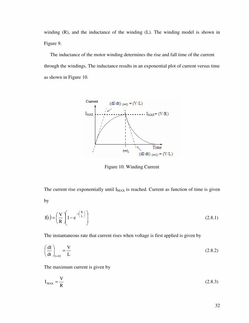
The inductance of the motor winding determines the rise and fall time of the current
through the windings. The inductance results in an exponential plot of current versus time
as shown in Figure 10.
Figure 10. Winding Current
The current rise exponentially until IMAX is reached. Current as function of time is given
by
( )��
�
�
��
�
�−�
�
���
�=��
���
�−LR
t
e1RV
tI (2.8.1)
The instantaneous rate that current rises when voltage is first applied is given by
( ) LV
dtdI
0t
=��
���
�
=
(2.8.2)
The maximum current is given by
RV
IMAX = (2.8.3)
33
The current in the winding will remain at IMAX until the supply is switched off. Referring
to Figure 10, the current drops exponentially when the voltage supply is removed.
Current as a function of time is then given by
( )( ) �
�
���
�−−
��
���
�= LR
TT 2
ERV
TI (2.8.4)
The instantaneous rate that the current drops when voltage is removed is given by
��
���
�−=LV
dtdI
(2.8.5)
These equations show that current rises and falls for a given winding as a function of the
supply voltage and internal winding resistance.
Referring to Equation (2.8.1) and (2.8.2), the rate that current rises in a winding is
increased by using a higher supply voltage. Equation (2.8.3) shows that IMAX is also
affected by increasing the supply voltage. So running a motor at high voltage while not
taking into consideration current limitations can be very detrimental to motor life and
drive circuitry.
2.9 Longevity
Another factor to consider when choosing a motor is the longevity of the motor. There is
no analytical method for calculating motor life. Motor life is a complex function of:
environment (temperature, altitude, humidity, air quality, shock, vibration, etc.), design
(commutation design, bearing design, etc.), and application variables (shaft loads,
velocity profile etc.).
Step motors by their nature are more robust than other type of motors because they do
not have brushes that will wear out over time. Typically, other components in a particular

34
system will wear out long before the motor. However, all step motors are not created
equal and even the best motors will fail if the proper considerations are not made. The
following are some design guidelines that influence motor longevity:
(1) Ball bearings last longer than bronze bushings and do not generate as much heat,
but they are more costly.
(2) Motors that run near their rated torque will not last as long as those that do not.
Motors should be chosen so that they will run at 40-60% of their torque rating.
(3) Protecting the motor from harsh environments. Exposure, humidity, harsh
chemicals, dirt and debris will decrease motor life.
(4) Ensuring adequate cooling will increase motor life and motor performance. Heat
sinking can have a dramatic effect not only on the motor, but also on the driven
load. Good design practice will allow for proper heat conduction away from
temperature sensitive machine members, as well as away from the motor. Hybrid
motors that use rare-earth magnets are particularly heat sensitive.
(5) A coupling method should be selected to prevent damage to the motor due to
axial or radial forces. Conversely, motor shaft end play, radial play and
concentricity should be considered to assure proper mating to the load.
(6) Resonance problems can be avoided by closely coupling all elements of the drive
train. Direct coupling is normally more economical, quieter and less prone to
resonance problems.
(7) Finally, motors should be driven properly. Special care should be taken to ensure
the current rating of the windings is not exceeded.

35
2.10 Resonance
Resonance is oscillatory phenomena which disturb the normal operation of the stepping
motor. In some cases the magnitude of oscillation increases with time and eventually the
motor loses synchronism. Resonance and instabilities may be classified into three
categories: low-frequency, medium-range instability, and higher-range oscillation.
2.10.1 Low-Frequency Resonance
When a stepping motor is started at a very low speed and the pulse frequency is increased
slowly, resonance first occurs at subharmonics of the natural frequency which is
ordinarily around 100 Hz. Then a major resonance will appear around the natural
frequency. These oscillations occur below 200 Hz and are called low-frequency
resonance. As the pulse rate is increased above the natural frequency, the magnitude of
oscillation decreases and becomes stable. In most practical situations the low-frequency
resonance does not critically limit the performance of the stepping motor system since
most motor/load combinations can be instantaneously started at stepping rates well above
the natural frequency.
2.10.2 Medium-Range Instability
When the stepping rate is increased to the range of 500 Hz to 1500 Hz, stepping motors
show troublesome behavioral features which are not of the low-frequency resonant type.
They are due to inherent instability in the motor or in the motor drive system. This kind
of oscillation in stepping motors is known as ‘medium-range instability.’ The frequency
of this oscillatory behavior is quite different from the natural frequency, but occurs at 1/4

36
to 1/5 of stepping rate. The region of mid-range can be crossed without loss of
synchronism by introducing more damping. Higher drive voltage and higher series
resistance of the step motor drive improves the performance of the step motor in the mid-
range frequency.
2.10.3 Higher-Range Oscillation
If the frequency is increased further and the motor is successfully accelerated through the
mid-range instability, the next region of instability occurs in the range of 2500 HZ to
4000 Hz which known as Higher-range Oscillation.
37
CHAPTER III
THE HARDWARE DESIGN OF THE SMC3
This chapter describes the various aspects of the SMC3 hardware. The SMC3 drive is
designed to drive a two-phase step motor. The SMC3 drive consists of four basic
elements: PWM-generator, power driver, sensing circuit, and DSP. The PWM-generator
generates two sinusoidal waveforms (for windings A and B) with frequencies and
amplitudes computed by the DSP. The sine waves are applied to the motor windings
through two full H-bridge power drivers. The full H-bridge driver provides bipolar drive
to the motor windings, connected between the positive and negative terminals. The sense
circuit measures motor winding voltages and currents. This chapter explains about
various techniques (sensor and sensorless) to sense rotor position. The sense motor
current is fed back to the DSP to implement current control. The SMC3 drive is built
using an ADSP-2101. This chapter explains the ADSP-2101 architecture, interrupts, and
serial ports.

38
3.1 SMC3 Design Overview
The SMC3 ECB (Electronic Circuit Board) is shown in Figure 11.
Figure 11. SMC3 ECB (Electronic Circuit board)
The SMC3 motor drive has been built using an Analog Devices ADSP-2101 digital
signal processor (DSP). The SMC3 is designed to work with two-phase step motors,
which are permanent magnet motors with many (typically 100) poles. The controller of
the SMC3 interfaces to the DSP via a serial interface. The DSP outputs duty-ratio values
to the dual PWM generator, which drives switching power drivers. These, in turn, drive
output circuits that interface to the motor windings. The SMC3 electronics (hardware)
functional diagram is shown in Figure 12.

39
The output sense circuits sense output voltages and currents. These analog quantities
are processed for input to the A/D converter. The control loop includes the DSP, which
inputs digitized voltage and current values from the motor. The DSP computes the output
quantity (torque or speed) and compares it with the commanded value. The error
difference is processed by a control filter to achieve the desired dynamic loop response.
The output quantities of the filter are duty ratios, D, that are sent to the dual PWM
generator via a DSP serial port.
Figure 12. SMC3 Hardware Functional Diagram
3.2 Dual PWM Generator
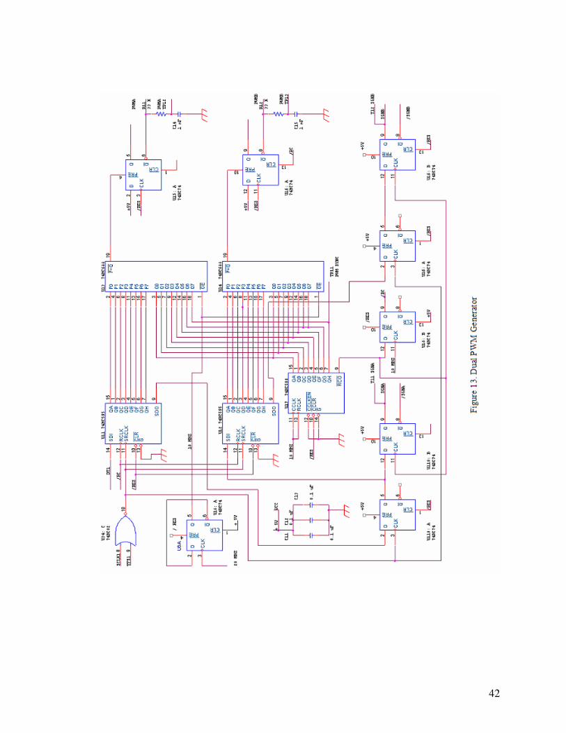
Figure 13 shows the dual PWM (pulse-width modulation) generator. The DSP generates
two sinusoidal waveforms (for windings A and B) with frequencies and amplitudes
computed by the DSP. The sine-waves are in PWM form, as signed PWM duty ratios.
The sine-waves are applied to the motor windings through two full H-bridge power
drivers (one for each winding). For smooth, steady-state motor operation, the two motor

40
windings voltages must be sine waves in quadrature. Each PWM on-time is represented
by nine bits (one sign bit and eight magnitude bits). DSP serial port 1 provides a
programmable, constant-frequency clock (SCLK1) that is gated by TFS1 (transmit frame
synchronization) for the 18 bits that are shifted into the shift registers of U11 and U12, in
that order. U11 and U12 are 74HC595s: 8-bit shift registers clocked on the SRCLK (shift
register clock input) pin, plus an 8-bit output register into which the shift-register is
clocked from the RCLK (storage register clock input) pin. U17 is an 8-bit counter that is
driven by a divide-by-two flip-flop, U18: A. The outputs of U11 and U12 are the PWMA
and PWMB duty-ratio values, respectively. The PWM magnitude is 8 bits, which is
compared against the U17 counter output by comparator U13. When the two comparator
inputs are equal, U13 pin 19 goes low, resetting flip flop U15/Q output low, and ending
the PWM cycle. The sign bit in the DSP code is considered positive when high.
Counter U17 Q7 output is brought out under the board on a wire that an oscilloscope
external sync probe can be connected to, called PWMA SYNC. It goes low at the end of
a PWM cycle, which is the beginning of a new PWM cycle. At the cycle transition point,
/RC of U18:B asserts, resetting the U15 flip-flops and setting the PWM pulses on (high)
at the /Q pins.
U17 is more than a counter. The 8 bits of the counter output drive an 8-bit register that
latches on RCLK input positive edges. Consequently, the output state at the Q0-Q7 pins
is one clock behind the counter. The /RCO output (pin 9) is the direct counter overflow,
which asserts low on count 254 of Q0-Q7. It is clocked into U18:B on the next clock, and
/RC asserts on count 255. Consequently the 255 state is the reset state and is not useable
as a valid PWM duty-ratio value. The PWM output is according to the duty-ratio formula

41
D = (N+1) / 256 , N = 0,……., 254 (3.2.1)
On count 255, /RC asserts low, resetting the U15:A PWM pulse and interrupting the
DSP through /IRQ2. Since the counter runs at 10 MHz, IRQ2 interrupts occur at a
frequency of 10 MHz / 256 = 39.0625 KHz. If N is set to 255, a very short PWM pulse
(of a few tens of nanoseconds) occurs. The shift-register output of U11 is the data input
(pin 14) of U12. Consequently, the PWMB value is shifted out of the DSP serial port
first.
To synchronize updating of D values with the PWM generator, the end of a PWMA
cycle interrupts the DSP, which then computes new values of D for PWMA and reissues
the current D value for PWMB. The composite 16-bit data stream is shifted out before the
end of the PWM cycle, so that when it occurs, the updated values of D are loaded into the
U11, U12 output registers at the 255 count (reload state), starting the new cycle. The
duty-ratio is a signed number of 9 bits. The sign bit switches the H-bridge for bipolar
drive, to create a sine-wave.
Because the serial port allows up to 16 bits, the 18-bit quantity is sent 9 bits at a time,
using the “transmit buffer empty” interrupt to effect transmission of the second PWM
quantity for PWM A. To avoid cyclic transmission, a flag variable is set upon the
transmission of the two PWM quantities.
For development and testing, it is hard to view a PWM waveform as a function of
time. To recreate an approximate waveform, the PWM output is low-pass filtered for
PWMA by R11 and C14, and is available at test point TP12. It normally appears as an
approximate (obviously sampled) magnitude of sine – a full-wave rectified sine wave.
Similarly, for PWMB, TP13 provides a filtered PWM representation.
42

43
3.3 Power Driver Circuit
The right half of Figure 14 is the power driver for PWMA (top) and an identical circuit
laid out on the circuit-board prototype for PWMB (bottom). The PWMA power driver is
a full H-bridge, with upper power switches Q21 and Q23, and low-side switches Q22 and
Q24. Either Q21 and Q24 are on and Q22 and Q23 off, or vice-versa, providing bipolar
drive to the load, connected between the A+ and A– terminals. This H-bridge uses
MOSFETs for one main reason - to improve the efficiency of the bridge. The voltage
drop across the collector and emitter can reach more than 1 V during saturation and high
heat dissipation is encountered using BJT devices. MOSFETS, which are intrinsically
characterized by low drain to source turn-on resistance, are better suited for motor drive
applications. MOSFETS are extremely static sensitive. If the gate is left open (no
connection) the MOSFET can self-destruct. The gate is a high impedance device (10+
megaohms) and noise can trigger the MOSFET. Resistors R23, R24, R25 and R26 have
been added specifically to stop the MOSFET from self-destructing. The TO-220
MOSFET package has a 1.7 °C/W thermal resistance.
The Power Integrations INT-201 high-side driver provides gate drive for an external
high-side MOSFET switch. It is used in conjunction with an INT-200 low-side driver.
This gate driver circuit provides a simple, cost effective interface between low voltage
control logic and high voltage load. For bipolar drive, SGNA and /SGNA select between
the + and – side low-side drivers and also gate the PWM waveform to the high-side
drivers (/HSI on the INT-200 ICs) using U21:A and :B NAND gates. The LSIN signal
directly controls Q21. The /HSIN signal causes the INT-200 to command the INT-201 to
turn Q22 on or off as required. The INT-200 will ignore input signals that would

44
command both Q21 and Q22 to conduct simultaneously, protecting against shorting high
bus to low bus.
The high-side driver INT-201 is designed to drive a floating N-channel MOSFET. The
bias voltage for the high-side driver is developed by a bootstrap supply circuit, consisting
of the diode and bootstrap capacitor. During start-up, the source (pin 5) is held at ground,
allowing CBOOT (C26) to charge to +15V through the diode (D22). When the PWM
input goes high, OUT (pin 6) will begin to charge the high-side MOSFET’s gate (Q21).
During this transition, charge is removed from CBOOT and delivered to Q21’s gate. As
Q21 turns on, the source (pin 5) rises to VIN, forcing the VDDH pin to VIN+VCBOOT which
provides sufficient VGS enhancement for Q21. To complete the switching cycle, Q21 is
turned off by pulling OUT (pin 6) to source. CBOOT is then recharged to VIN. When OUT
(pin-5) falls to ground, OUT is in phase with PWM input.
The low-side driver (INT-200) is designed to drive a ground referenced low RDS(ON)
N-channel MOSFET. The bias for the low-side driver is connected between the OUT pin
and ground. When the driver is enabled, the driver’s output is 1800 out of phase with the
PWM input.

45
46
3.3.1 PWM Switching Technique
For the SMC3 system the supply voltage is chopped at a fixed frequency (39.0625 KHz)
with a duty cycle depending on the reference input (potentiometer). The main advantage
of this PWM strategy is that the chopping frequency is a fixed parameter; hence acoustic
and electromagnetic noise is relatively easy to filter [5]. There are two ways of handling
the drive current switching: hard chopping and soft switching.
In hard chopping both transistors are driven by the same pulsed signal: the two
transistors are switched on and switched off at the same time. In soft chopping mode the
low side transistor is left on during the phase supply and high side transistor switches
depending on the duty cycle set by the reference input. The soft chopping approach
allows not only control of the current and of the rate of change of the current but
minimization of the current ripple as well. The rate of current change is related directly to
the voltage applied across the winding by the equation
V = L (di/dt) (3.3.1)
The current ripple will be determined by the chopping frequency and the voltage across
the coil [6]. When the winding is driven by two transistors switched on, the voltage
across the winding is fixed by the power supply minus the saturation voltage (RDon
voltage drop) of the MOSFET. When soft switching is used, the voltage across the
winding during recirculation is Von of the lower transistor plus one diode drop plus the
voltage drop across the sense resistor. In this case the current decays much slower than it
rises and the ripple current is much smaller than in the previous case. So for this reason
SMC3 uses the soft switching technique.

47
3.3.2 Maximum Current Limiter U23A (LM393) is used to provide current limiting in the SMC3. The way this circuit
works is that the voltage across the current sense resistor (Rsense) is compared with a fixed
reference voltage which is predetermined according to
Vref = Rsense * IMAX (3.3.2)
When Vsense rises above Vref the transistor to which the PWM is applied is put in the
off state until the current feedback becomes less than the maximum current limit. So one
of the inputs to the LM393 comparator is the maximum current limit (set by VRH, R216,
and R217), and the other input is the current feedback form the motor [7].
A comparison of the current and the voltage applied to the winding over time is
showing in Figure 15. The current limit can be changed by changing R216 or R217. This
current limit is for protection and normally it is not reached.
Figure 15. Winding Current and Supply Voltage
48
3.4 Sensing Circuit
The sensing circuits are on the left half of Figure 14. The output sense circuits measure
motor winding voltages and currents. The winding voltage zero crossings are detected
and input to the DSP as comparator output waveforms, and the currents are measured as
scaled analog voltage. These voltages are input to an Analog Devices AD7811 ADC. The
ADC outputs are sent to the serial port 0 (SPORT0) input of the DSP. The SPORT0
output simultaneously sets the channel for the next A/D sample acquisition.
3.4.1 Zero-Crossing Detection
The first step in the development of a sensorless motor control is the detection of the
motor back emf. The back emf is created when the motor’s rotor turns, which creates an
electrical kickback or emf that is sensed as a voltage through the resistor. The amplitude
of the emf signal increase with the speed of the rotation. The back emf voltage produces a
sine waveform that is sensed and converted to a digital square wave by a zero-crossing
circuit. The comparator signal is input to the DSP, which calculates the commutation
sequence and motor position from the phase relationship of the square wave
representation of the back emf signals.
A limitation of the back emf method is that the amplitude of the signal is very small at
low shaft speed. So for that reason the back emf signal is amplified before comparing it
with a fixed reference. The back emf measured from the winding is noisy and small in
amplitude. So first it is filtered and amplified by U22:A. Low pass filtering helps to
restrict the bandwidth to frequencies close to the frequency of the signal being measured
[8]. This technique is well suited for signals that are expected to have small deviations
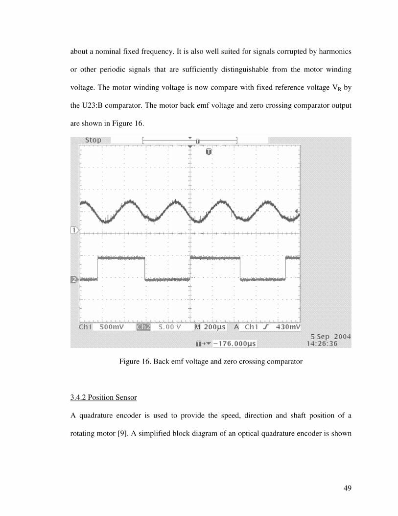
49
about a nominal fixed frequency. It is also well suited for signals corrupted by harmonics
or other periodic signals that are sufficiently distinguishable from the motor winding
voltage. The motor winding voltage is now compare with fixed reference voltage VR by
the U23:B comparator. The motor back emf voltage and zero crossing comparator output
are shown in Figure 16.
Figure 16. Back emf voltage and zero crossing comparator
3.4.2 Position Sensor
A quadrature encoder is used to provide the speed, direction and shaft position of a
rotating motor [9]. A simplified block diagram of an optical quadrature encoder is shown

50
in Figure 17. The typical quadrature encoder is packaged inside the motor assembly and
provides three logic-level signals.
A quadrature encoder generates two signals that are electrically 90 degrees out of
phase with each other. The term quadrature refers to this 90 degrees phase relationship.
Motor speed is determined by the frequency of the Channel A and B signals. The phase
relationship between Channel A and B can be used to determine if the motor is turning in
either the forward or reverse direction. The index signal provides the position of the
motor. A single pulse is generated for every 360 degrees of the shaft rotation.
Figure 17. Position Sensor
3.4.3 Current Sensing
Shunt resistors are a popular current-sensing device because of their low cost and good
accuracy. The current flowing through the resistor will be proportional to the voltage
drop across it. Measuring the voltage drop across it gives an indication of the current flow
in the motor. This resistor is small in magnitude, making as little impact on the circuit as
possible; if it is too high in value it will eat up a considerable amount of power.

51
Shunt resistors can provide either high-side or low-side measurements of the current
flowing through the motor. A high-side monitor has the resistor connected in series with
the power source, while a low-side monitor locates the resistor between the load and the
ground current return path. The SMC3 uses the low-side measurement method. Low-side
current measurement offers the advantage that the circuitry can be implemented with a
low voltage op-amp because the measurement is referenced to ground. A simplified
version of the current measurement used in the SMC3 is shown in Figure 18.
VIA = (Vsense)*(1+2000/220)
VIA = IA*0.1*14.3
VIA = IA*1.43
So the scaling for the current measured as a scaled analog voltage is 1.43.
Figure 18. Current Sensing Circuit

52

53
3.5 Speed Input
The DSP and speed input circuit is shown in Figure 19. The potentiometer input can be
varied between -10 V to +10 V. The input range of the A/D converter is 0 V to 5 V. In
order to make the potentiometer input compatible with the A/D converter, a differential
amplifier (LM324) with a feedback resistance of 6.8 k is used.
Figure 20. Speed Command Interface
As seen from Figure 20 the input available at pin number 10 of the differential
amplifier is [(10/10+23.2)*Vspd+3.149] = [(0.3012)*Vspd+3.149]. This input voltage is
buffer by a differential amplifier. Before applying this voltage to the A/D converter, a
voltage divider circuit with a resistance of 10 k and 26.7 k is used. So input of A/D
converter (X) is given by
X = [Vspd*(0.3012)+3.149]*(26.7/(26.7+10)] (3.5.1)
Output of the A/D converter (W) is
W= [Vspd*(0.3012)+3.149]*(0.7275)*(1024/4.506)

54
W= [(49.8*Vspd)+ 520.6] (3.5.2)
The potentiometer input and corresponding ADC count for different input values is given
in Table 2.
Table 2. Potentiometer Input and Corresponding ADC Count
3.5.1 AD7811 A/D Converter
The AD7811(U36) is a four-channel analog to digital converter with a conversion rate of
2.3 �s. The maximum input voltage is 5 V and the minimum input voltage is 0 V. It is a
10 bit A/D converter, so each bit will represent = (5 – 0) / 1024 = 4.88 mV [10]. Channel
0 is connected to the potentiometer input. Channel one and two are connected to the
output of the LM358, which is the current measured as a scaled analog voltage of
windings A and B respectively. Channel three is connected to the winding supply
voltage.
3.5.2 Reference Voltage
A stable reference voltage of 4.506V is required in the SMC3. This reference voltage is
Potentiometer Input
LM324 Input Vspd*(0.3012)
+ 3.149
AD7811 Input [Vspd*(0.3012)+3.149] *
(0.7275)
ADC Count
Ideal Count
+ 10 V 6.161 V 4.482V 1019 1023
0 V 3.149 V 2.291 V 521 512
-10 V 0.137V 30.9 mV 7 0

55
independent of supply voltage variations and shows minimum sensitivity to temperature.
This constant voltage reference is used for the zero crossing detection circuit for the back
emf. The input to U35:B (LM324) is 4 V. So the available reference voltage at pin 7 is
Vref = 4 * (1+ 30.1/(100+191))
Vref = 4.506V. (3.5.3)
A voltage divider circuit is composed of R311 and R312 to divide the reference voltage
by half which is buffered by U35:A (LM324). This voltage is used for setting the
maximum current limit in the motor.
3.5.3 External latch
The U34:B and :A form an OR gate that gates U33 onto the DSP external bus for read
cycles addressing data memory (/DMS asserted). U33 inputs have been modified to be
available at the square-pin connector, as indicated in the photograph of the ECB (Figure
11). Eight bits are available externally from a 74HC373 latch. Pins 1 and 2 are the 5 V
supply and ground, and pins 3-8 are D0-D5 of the U33 tri-state 8-bit buffer. Bits D6 and
D7 come from the configuration jumpers on the board, for selection of code segments in
program boot memory. These eight bits include three encoder bits (two quadraturer bits
and an absolute position index bit), two phase-winding zero-crossing bits, a stop-
command bit that can be asserted with a pushbutton, and two configuration jumpers.
U37 is the DSP reset circuit. It also clocks the PWM flip-flops 74HC74 (U15) at reset
to low outputs (no drive). U32 is a 27128 EPROM containing the program code for the
DSP. At reset, the DSP boots in the program code and then proceeds to execute it.
Multiple programs can be selected and loaded from EPROM to the ADSP-2101.
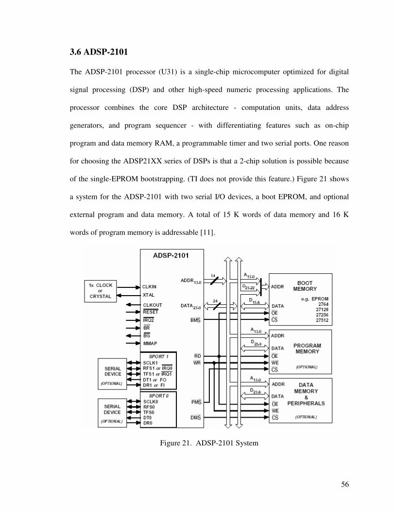
56
3.6 ADSP-2101
The ADSP-2101 processor (U31) is a single-chip microcomputer optimized for digital
signal processing (DSP) and other high-speed numeric processing applications. The
processor combines the core DSP architecture - computation units, data address
generators, and program sequencer - with differentiating features such as on-chip
program and data memory RAM, a programmable timer and two serial ports. One reason
for choosing the ADSP21XX series of DSPs is that a 2-chip solution is possible because
of the single-EPROM bootstrapping. (TI does not provide this feature.) Figure 21 shows
a system for the ADSP-2101 with two serial I/O devices, a boot EPROM, and optional
external program and data memory. A total of 15 K words of data memory and 16 K
words of program memory is addressable [11].
Figure 21. ADSP-2101 System

57
Figure 22 shows a block diagram of the ADSP-2101 architecture. The processors
contain three independent computational units: the ALU, the multiplier/accumulator
(MAC), and the shifter. The computational units process 16-bit data directly and have
provisions to support multiprecision computations. The ALU performs a standard set of
arithmetic and logic operations; division primitives are also supported. The MAC
performs single-cycle multiply, multiply/add, and multiply/subtract operations. The
shifter performs logical and arithmetic shifts, normalizations, demoralization, and derive
exponent operations. The shifter can be used to efficiently implement numeric format
control including multiword floating-point representations.
Figure 22. ADSP-2101 Block Diagram
3.6.1 Data Transfer
The internal result (R) bus directly connects the computational units so that the output of
any unit may be used as the input of any unit on the next cycle. A powerful program
sequencer and two dedicated data address generators ensure efficient use of these
58
computational units. Two data address generators (DAGs) provide addresses for
simultaneous dual operand fetches. Each DAG maintains and updates four address
pointers. The circular buffering feature is also used by the serial ports for automatic data
transfer to on-chip memory.
Efficient data transfer is achieved with the use of five internal buses:
• Program Memory Address (PMA) Bus
• Program Memory Data (PMD) Bus
• Data Memory Address (DMA) Bus
• Data Memory Data (DMD) Bus
• Result (R) Bus
The two address buses (PMA, DMA) share a single external address bus, allowing
memory to be expanded off-chip, and the two data buses (PMD, DMD) share a single
external data bus. The BMS, DMS, and PMS signals indicate which memory space is
using the external buses. The memory interface supports slow memories and memory-
mapped peripherals with programmable wait state generations. External devices can gain
control of the processor’s buses with the use of the bus request/grant signals (BR, BG).
3.6.2 Serial Ports
The ADSP-2101 processor includes synchronous serial ports (“SPORTs”) for serial
communications and multiprocessor communication. The ADSP-2101 processor has two
serial ports (SPORT0, SPORT1). SPORT0 is used to take data in from the A/D converter
and SPORT1 is used to transmit PWM data to the PWM generator circuit for windings A
and B. A wide variety of framed or frameless data transmit and receive modes of

59
operation are available on the serial ports. Each SPORT can generate an internal
programmable serial clock or accept an external serial clock. The serial clock is generated
internally on both serial ports in the SMC3. SPORT0 provides a multichannel interface to
selectively receive or transmit a 24-word or 32-word, time-division multiplexed serial bit
stream. SPORT0 is used to select one channel from the four-channel A/D converter. Each
serial port has a 5-pin interface consisting of the signals given in Table 3. Writing to a
SPORT’s TX register readies the SPORT for transmission; the TFS signal initiates the
transmission of serial data. Once transmission has begun, each value written to the TX
register is transferred to the internal transmit shift register and subsequently the bits are
sent, MSB first. Each bit is shifted out on the rising edge of SCLK. After the first bit
(MSB) of a word has been transferred, the SPORT generates the transmit interrupt. The
TX register is now available for the next data word, even though the transmission of the
first word is ongoing. In the receiving section, bits accumulate as they are received in an
internal receive register. When a complete word has been received, it is written to the RX
register and the receive interrupt for that SPORT is generated.
Signal Name Function
SCLK Serial Clock (I/O)
RFS Receive Frame Synchronization (I/O)
TFS Transmit Frame Synchronization (I/O)
DR Serial Data Receive
DT Serial Data Transmit
Table. 3 Interface Signal

60
3.6.3 Interrupts
The ADSP-2101 processor can respond to several different interrupts. Three external
interrupt input pins, IRQ0, IRQ1, and IRQ2, are available. IRQ2 is always available as a
dedicated pin; IRQ1 and IRQ0 may be alternately configured as part of Serial Port 1. The
ADSP-2101 also supports internal interrupts from the timer, and the serial ports. The
interrupts are internally prioritized and individually maskable (except for RESET which
is non-maskable). The IRQx input pins can be programmed for either level- or edge-
sensitivity. In the SMC3 the IRQx input pins are programmed for edge sensitivity. The
ADSP-2101 processor can provide either: one external interrupt (IRQ2) and two serial
ports (SPORT0, SPORT1), or three external interrupts (IRQ0, IRQ1, IRQ2) and one
serial port (SPORT0). In the SMC3 IRQ0 and IRQ1 are not used because SPORT1 is
configured as a serial port. IRQ2 is generated from external PWM counter overflow,
which occurs every 25.6 �s. A programmable interval timer can generate periodic
interrupts. A 16-bit count register (TCOUNT) is decremented every n cycles, where n-1
is a scaling value stored in an 8-bit register (TSCALE). When the value of the counter
register reaches zero, an interrupt is generated and the count register is reloaded from a
16-bit period register (TPERIOD). In the SMC3 TSCALE is fixed to 0 and TPERIOD is
fixed to 199. So the timer interrupt comes every 10 �s.
When an interrupt request occurs, it is latched while the processor finishes executing
the current instruction. The interrupt request is then compared with the interrupt mask
register (IMASK), by the interrupt controller. If the interrupt is not masked, the program
sequencer pushes the current value of the program counter (which contains the address of
the next instruction) onto the PC stack. This allows execution to continue, after the

61
interrupt is serviced, with the next instruction of the main program. The program
sequencer also pushes the current values of ASTAT, MSTAT, and IMASK register onto
status stack. ASTAT, MSTAT, and IMASK are stored in this order, with the MSB of
ASTAT first, and so on. When IMASK is pushed, it is automatically reloaded with a new
value that determines whether or not interrupt nesting is allowed. The processor then
executes a NOP while simultaneously fetching the instruction located at the interrupt
vector address. Upon return from the interrupt service routine, the PC and status stacks
are popped and execution resumes with the next instruction of the program.
3.6.4 System Clock
The ADSP-2101 processor’s CLKIN input may be driven by a crystal or by a TTL-
compatible external clock signal. The CLKIN input may not be halted or changed in
frequency during operation, nor operated below the specified low frequency limit.
Because the ADSP-2101 processor includes an on-chip oscillator circuit, an external
crystal may also be used. In the SMC3 an external crystal is used which is mounted on
the ECB bottom side. The crystal is connected across the CLKIN and XTAL pins, with
two capacitors connected as shown in Figure 23. A parallel-resonant, fundamental
frequency, microprocessor-grade crystal is used.
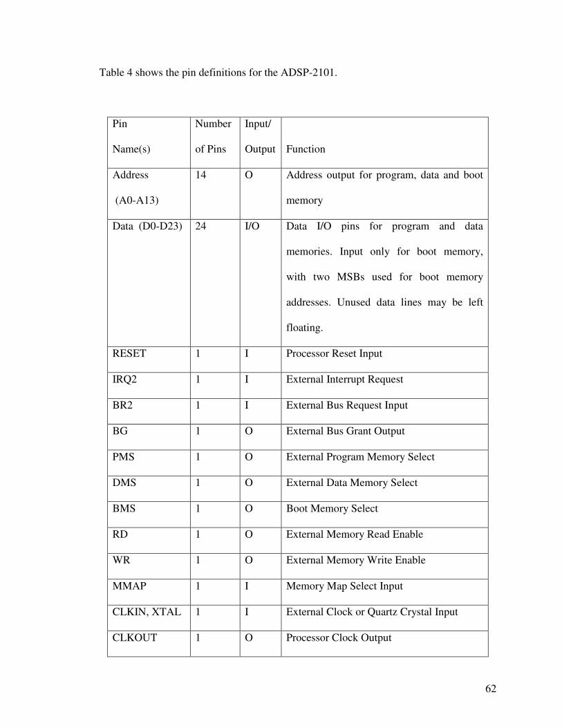
62
Table 4 shows the pin definitions for the ADSP-2101.
Pin
Name(s)
Number
of Pins
Input/
Output
Function
Address
(A0-A13)
14 O Address output for program, data and boot
memory
Data (D0-D23) 24 I/O Data I/O pins for program and data
memories. Input only for boot memory,
with two MSBs used for boot memory
addresses. Unused data lines may be left
floating.
RESET 1 I Processor Reset Input
IRQ2 1 I External Interrupt Request
BR2 1 I External Bus Request Input
BG 1 O External Bus Grant Output
PMS 1 O External Program Memory Select
DMS 1 O External Data Memory Select
BMS 1 O Boot Memory Select
RD 1 O External Memory Read Enable
WR 1 O External Memory Write Enable
MMAP 1 I Memory Map Select Input
CLKIN, XTAL 1 I External Clock or Quartz Crystal Input
CLKOUT 1 O Processor Clock Output
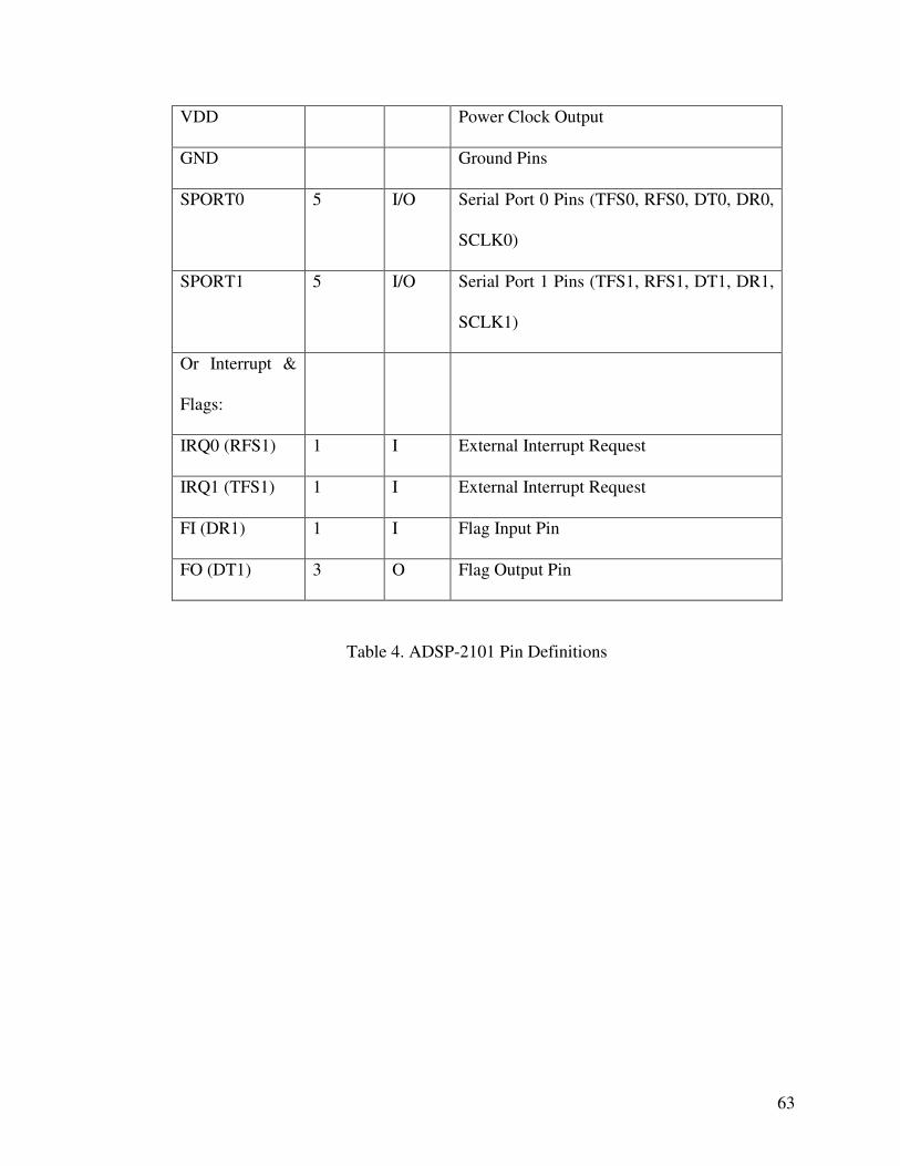
63
VDD Power Clock Output
GND Ground Pins
SPORT0 5 I/O Serial Port 0 Pins (TFS0, RFS0, DT0, DR0,
SCLK0)
SPORT1 5 I/O Serial Port 1 Pins (TFS1, RFS1, DT1, DR1,
SCLK1)
Or Interrupt &
Flags:
IRQ0 (RFS1) 1 I External Interrupt Request
IRQ1 (TFS1) 1 I External Interrupt Request
FI (DR1) 1 I Flag Input Pin
FO (DT1) 3 O Flag Output Pin
Table 4. ADSP-2101 Pin Definitions
64
CHAPTER IV
CURRENT CONTROL IN STEP MOTORS
Sensorless motor control obtains the speed and position of the motor directly from the
voltage of the motor winding. If the sources across motor windings appear as voltage
sources, then the sensed winding voltage is just the output of H-bridge, not the induced
voltage. If the winding current is controlled then the sources driving the motor windings
appear as current sources rather than voltages sources, which allows sensing of the motor
induced voltages across the windings to obtain their zero-crossings for sensorless motor
control. In this chapter the transfer function of the step motor is derived and various
motor parameters are calculated. This information is used to simulate the SMC3 system
using Matlab Simulink to find proper the tuning parameters of a PID controller for
current control, and simulation results are compared with experimental results.
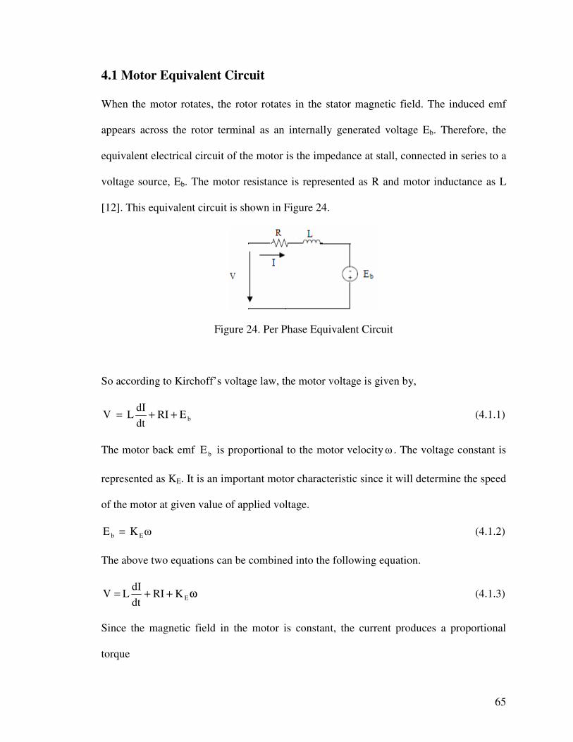
65
4.1 Motor Equivalent Circuit
When the motor rotates, the rotor rotates in the stator magnetic field. The induced emf
appears across the rotor terminal as an internally generated voltage Eb. Therefore, the
equivalent electrical circuit of the motor is the impedance at stall, connected in series to a
voltage source, Eb. The motor resistance is represented as R and motor inductance as L
[12]. This equivalent circuit is shown in Figure 24.
Figure 24. Per Phase Equivalent Circuit
So according to Kirchoff’s voltage law, the motor voltage is given by,
V = bERIdtdI
L ++ (4.1.1)
The motor back emf bE is proportional to the motor velocity� . The voltage constant is
represented as KE. It is an important motor characteristic since it will determine the speed
of the motor at given value of applied voltage.
bE = �K E (4.1.2)
The above two equations can be combined into the following equation.
ω++= EKRIdtdI
L V (4.1.3)
Since the magnetic field in the motor is constant, the current produces a proportional
torque
66
T = IK T (4.1.4)
The constant friction torque can be represent as fT and the viscous friction torque which
is proportional to the velocity can be represent as D� . The opposing torque in the motor,
mT , is given by
mT = D�Tf + (4.1.5)
If motor is coupled to a load, the relation between torque and velocity is given by
T = ( ) LfLm TTD�dtd�
jj ++++ (4.1.6)
where Lj represent the load moment of inertia, mj represent the rotor moment of inertia,
and LT represent the load opposing torque.
The above equation is the dynamic equation of the motor, and it describes the relation
between the electrical and mechanical variables.
4.1.1 Motor Transfer Function
When the motor is used as a component in a system, it is desired to describe it by the
appropriate transfer function between the motor voltage and its velocity. For this purpose
assume TL=0 and Tf=0, since neither affects the transfer function. If we now apply a
Laplace transformation to the motor equations, we get:
( )sV = ( ) ( ) ( )sKsIRsL Eω++ (4.1.7)
( )sT = ( )sIK T (4.1.8)
T(s) = ( ) ( ) ( )sDssjj Lm ω+ω+ (4.1.9)
The total moment of inertia J is given by
J = Lm jj + (4.1.10)

67
By using equation (4.2.2) and (4.2.3) we obtain an expression for the current:
( )sI = ( ) ( )s�DsJK1
T
+���
����
� (4.1.11)
Combine Equation (4.1.11) and Equation (4.1.7) to form
( )sV = ( )( ) ( ) ( )s�Ks�DsJRsLK1
ET
+++ (4.1.12)
The corresponding transfer function is
( )sG m = ( )( )sVs�
(4.1.13)
= ( )( ) TE
T
KKDsJRsLK
+++ (4.1.14)
The motor impedance is given by;
( )sZ = ( )( )sIsV
= ( )( ) ( )
( )DsJKKs�DsJRsL TE
++++
(4.1.15)
The torque constant is always related to the voltage constant in the following way:
TK = EK ��
�
�
ANm
(4.1.16)
By using proper units for the torque constant, the motor impedance is given by
( )sZ = ( )( )sIsV
= ( )( ) ( )
( )DsJKs�DsJRsL 2
T
++++
(4.1.17)
4.1.2 Torque Constant
The torque constant is measured by operating the motor as a generator at a constant
velocity [13]. The torque constant is given by the following relationship
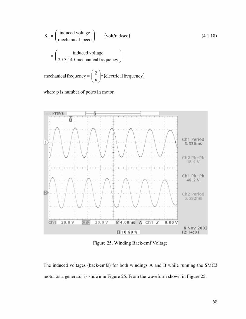
68
TK = ���
����
�
speed mechanical voltageinduced
( )ecvolt/rad/s (4.1.18)
= ���
����
�
∗∗ frequency mechanical14.32 voltageinduced
frequency mechanical = ( )frequency electrical2 ∗���
����
�
p
where p is number of poles in motor.
Figure 25. Winding Back-emf Voltage
The induced voltages (back-emfs) for both windings A and B while running the SMC3
motor as a generator is shown in Figure 25. From the waveform shown in Figure 25,

69
frequency mechanical = ��
���
�∗��
���
�
00574.01
1002
= 484.3
So torque constant for SMC3 motor is obtained as
TK = ( )����
���
�
∗∗ 484.314.321.24
TK = 1.01 ��
�
�
ANm
(4.1.19)
4.1.3 PID Controller
The PID controller looks at the current value of the error, the integral of the error over a
recent time interval, and the current derivative of the error signal, to determine how much
of a correction to apply and for how long. Each of those three quantities are multiplied
by a tuning constant and added together. Thus the PID output u(t) is a weighted sum as
explained by following equation.
( )tu = PK e + eK I td +dtde
K D (4.1.20)
By adjusting the weighting constants Kp, KI, and KD, the PID controller can be set to give
the desired performance.
As explained so far, continuous time domain and analog variables are considered in
PID control. In the SMC3, the PID algorithms have been implemented in DSP. This
means that the PID controller operates in discrete time and deals with analog signals
quantized to a limited number of levels. To discretise the controller, the integral and
derivative terms of the controller have to be approximated. The integral becomes a sum

70
and the derivative becomes a difference. The continuous time signal e(t) is sampled at a
sample period T. Thus discrete PID control can be described by the following equation.
( )tU = PK ( )te + IK T ( )� ne + ( ) ( )[ ]1kekeK D −− (4.1.21)
4.2 SMC3 Open-Loop Simulink Model
Figure 26. SMC3 Open-Loop Model
The SMC3 open-loop Simulink model is shown in Figure 26 [14]. The potentiometer is
used to set the reference quantity (speed or torque). The potentiometer inputs to the DSP.
The DSP generates two sinusoidal waveforms with frequencies and amplitudes computed
by the DSP. The sine waves are in PWM form as PWM duty ratios. The sine waves are
applied to the motor windings through two full H-bridge power drivers (one for each
winding). The motor current is measured as a scaled analog voltage which is the output of
the LM293 amplifier.

71
4.2.1 SMC3 Closed-Loop Model
Figure 27. SMC3 Closed-Loop Model
The model shown in Figure 27 is an equivalent hardware configuration for the current
controller, which has been implemented in software inside the DSP. In this control
method the magnitude of the current flowing into the winding is controlled using a
control loop with current feedback. The current in a motor phase winding is directly
measured with a current sense resistor connected in series with the phase. The pulse
width modulation (fixed frequency of 39.0625 KHz) signals with varying duty cycle is
used for current regulation. The current is compared with a desired value of current
(potentiometer reference), forming an error signal. The current error is compensated via
the PID regulator, and an appropriate control action is taken as shown below
errorI = fbref II − (4.2.1)
newduty_cycle = oldcycleduty − + ( )1kKp EEK −− (4.2.2)
If ≥newduty_cycle max_duty
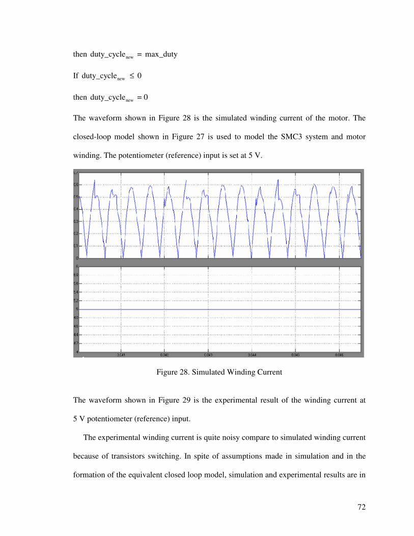
72
then newduty_cycle = max_duty
If newduty_cycle ≤ 0
then newduty_cycle = 0
The waveform shown in Figure 28 is the simulated winding current of the motor. The
closed-loop model shown in Figure 27 is used to model the SMC3 system and motor
winding. The potentiometer (reference) input is set at 5 V.
Figure 28. Simulated Winding Current The waveform shown in Figure 29 is the experimental result of the winding current at
5 V potentiometer (reference) input.
The experimental winding current is quite noisy compare to simulated winding current
because of transistors switching. In spite of assumptions made in simulation and in the
formation of the equivalent closed loop model, simulation and experimental results are in

73
close agreement. The average (and peak) values of the winding currents (experimental
and simulated) matches reasonably well, which is important in terms of PID controller
tuning.
Figure 29. Experimental Winding Current
4.2.2 PID Controller Tuning
Proportional action is typically the main drive in a control loop. The proportional gain,
Kp, reduces a large part of the overall error. Kp provides the instantaneous error correction
and is independent from the sampling time value. The higher the Kp, the lower will be the
error and the better will be the dynamic response. Taking a very high value for Kp will

74
oscillate the system. Proportional action alone can not reduce the steady-state error. The
value of proportional gain of 0.1 provides satisfactory results for SMC3 current control.
The dynamic response of the system is fast enough and steady-state error is not that high.
Integral action reduces the final error in a system. Summing even a small error over
time produces a drive signal large enough to move the system towards a smaller error.
The higher the integral gain KI, the faster will be the error cancellation and the better will
be the dynamic response. The SMC3 system is not using integral control. Adding integral
control will reduce steady-state error but at same time will increase the response time of
the system.
Derivative action speeds up the system response by adding in control action
proportional to the rate of change of feedback error. Consequently this is susceptible to
noise in the error signal, which limits derivative gain. The SMC3 system is not using
derivative action.

75
CHAPTER V
SENSORLESS STEP MOTOR CONTROL
The sensed winding current is quite noisy because of the switching transistors. So better
current estimation can be obtained by using a Kalman filter. In order to implement
sensorless step motor control it is necessary to know the position of the rotor. The DSP
can compute rotor position using sophisticated rotor-position estimation algorithms, such
as a Kalman filter that extracts estimates of the rotor position from measurements of the
motor voltage and current [15-16]. This estimator relies on the real time implementation
of a sufficiently accurate model of the motor in the DSP. This chapter describes in brief
the Kalman filter and its application for sensorless control of the SMC3 system.
5.1 Kalman Filter
The Kalman filter was developed by R.E. Kalman in 1960 [17]. Due to advances in the
development of digital computing, the Kalman filter is a subject of extensive research and
application. Kalman filtering has been applied in the areas of aerospace, navigation,
manufacturing, and many others.
76
The Kalman filter provides a means for inferring missing information from indirect
(and noisy) measurements. It provides the optimal (minimum variance) state estimate
when the dynamic system is linear and the statistical characteristics of the various noise
elements are know [18]. The system can be described with following equation.
x� = BwBuAx ++ (System) (5.1.1)
y = Cx+ Dv (Measurement) (5.1.2)
where x is the state, y is the measurement, u is the control input, and w and v are the
system and measurement noise. The measurement vector could be a function of the
control as well as the state. The assumptions regarding the noises are that these noises are
stationary, white, uncorrelated, and their expectation is zero. The definition of the
covariance matrices of these noises is:
( ) { } QwwEwcov T == (5.1.3)
( ) { } RvvEvcov T == (5.1.4)
where E{.} denotes expected value.
The overall structure of the Kalman filter leads to the system equation:
( ) KyBuxKCAx ++−=� (5.1.5)
where K denotes the Kalman gain matrix. The setting of the matrix K depends on the
covariance of the noises.
The quality of measurement of the goodness of the observation is given by;
( ) ( ){ } −−= dtxxxxminEH T (5.1.6)
H can be minimized by choosing K as;
K = PCTR−1 (5.1.7)
where P can be calculated from the solution of the following equation:

77
PCTR−1 CP- AP- PAT – Q = 0 (5.1.8)
Q and R have to be set up based on the stochastic properties of the corresponding noises.
Since these are usually not known, they are used as weight matrices in most cases.
5.1.1 Discrete-Time Kalman filter
The discrete-time linear system can be modeled as;
xk = Ak-1xk +Buk-1 +wk-1 (5.1.9)
The measurement equation can be modeled as;
yk = Ckxk+vk (5.1.10)
where k is the time index.
The system noise is white and zero-mean:
E(wk)=0 (5.1.11)
E(wkwTk)=Qk (5.1.12)
E(wkwTj)=0 (k�j) (5.1.13)
The measurement noise is white, zero-mean, and uncorrelated with the system noise:
E(vk)=0 (5.1.14)
E(vkvTk)=Rk (5.1.15)
E(vkvTj)=0 (k�j) (5.1.16)
E(vkwTj)=0 (5.1.17)
The discrete-time Kalman filter recursive generation can be expressed in five equations:
(1) State Estimate Extrapolation (Propagation)
(2) Covariance Estimate Extrapolation (Propagation)
(3) Filter Gain Computation

78
(4) State Estimate Update
(5) Covariance Estimate Update
The discrete-time Kalman filter can be implemented as follows:
State estimate extrapolation:
1k1k1k1k1k/k uBxAx −−−−− += (5.1.18)
Covariance estimate extrapolation:
1kT
1k1k1kT
11/kk1k1k/k BQBAPAP −−−−−−−− += (5.1.19)
Kalman filter gain:
1k1k
T1kk1k1k
T1kkk ]RCPC[CPK −
−−−−− += (5.1.20)
State estimate update:
]xCy[Kxx 1kk1kkk1kkk −−− −+= (5.1.21)
Covariance estimate update:
11k
1k1k
T11k/kk/k ]CRC[PP −
−−
−−
− += (5.1.22)
The 1kkx − denotes the state estimate that results from the propagation equation alone,
1kx − is the correlated state estimate that accounts for the measurements and 1kkP − and kP
are defined similarly.
5.1.2 Extended Kalman Filter (EKF)
The extended Kalman filter is used if the process to be estimated or the measurement
relationship to the process is non-linear. The extended Kalman filter retains the linear
calculation of the covariance and the Kalman gain matrices, and it updates the state
estimate using a linear function of a filter residual using original nonlinear equations for

79
state propagation and definition of the output vector. The extended Kalman filter
linearizes about the current mean and covariance.
Assuming the system has a state vector x and the system is governed by the non-linear
difference equation
( )1k,1k1kk wu,xfx −−−= (5.1.23)
with the measurement y which is
( )kkk v,xhy = (5.1.24)
In practice, it is not possible to know the value of the process noise wk-1 and measurement
noise vk-1 at each time step and we can still estimate the state without them as
( )0u,xfx ,1k1kk −−=
( )0,xhy 1-kk =
The extend Kalman filter can be expressed as;
State estimate extrapolation:
( ),0u,xfx 1k1k1kk −−− = (5.1.25)
( ) 1k1k1k1-k1k1k uBxA,0u,xf −−−−− += (5.1.26)
Covariance estimate extrapolation:
Qx
fP
xf
P1k1k1k1k xx
T
1k
xx
T
1kk +∂
∂∂
∂=−−−− =
−=
− (5.1.27)
where Q represents the system noise covariance matrix and it is defined as
Q = E(wkwTk)
Kalman filter gain computation:
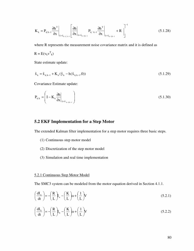
80
1
xx
T
1kkxxxx
T
1kkk Rx
hP
xh
xh
PK1k1k1k1k1k1k
−
=−
==−
��
�
�
�+
∂∂
∂∂
∂∂=
−−−−−−
(5.1.28)
where R represents the measurement noise covariance matrix and it is defined as
R = E(vkvTk)
State estimate update:
))0,x(hy(Kx x 1kkkk1kkk −− −+= (5.1.29)
Covariance Estimate update:
��
�
�
��
�
�
∂∂−=
−−= 1k1kxxkkk x
hKIP (5.1.30)
5.2 EKF Implementation for a Step Motor
The extended Kalman filter implementation for a step motor requires three basic steps.
(1) Continuous step motor model
(2) Discretization of the step motor model
(3) Simulation and real time implementation
5.2.1 Continuous Step Motor Model
The SMC3 system can be modeled from the motor equation derived in Section 4.1.1.
VL1
�LK
ILR
dtdI
aa �
�
���
�+��
���
�−��
���
�−=��
���
� (5.2.1)
VL1
�LK
ILR
dtdI
bb �
�
���
�+��
���
�−��
���
�−=��
���
� (5.2.2)

81
�JD
IJK
dtd�
a ��
���
�−��
���
�=��
���
� (5.2.3)
�dtd� =��
���
� (5.2.4)
The system can be modeled as;
����
�
�
�
�
�
II
dtd b
a
=
��������
�
�
�
��
���
�−��
���
�
��
���
���
���
�−��
���
�−
��
���
���
���
�−��
���
�−
0100
0JD
0JK
L1
LK
LR
0
L1
LK
0LR
����
�
�
�
�
�
II
b
a
+
�������
�
�
�
��
���
�
��
���
�
00L1L1
V (5.2.5)
We are measuring current Ia and Ib.
��
�
�
b
a
II
= ��
�
�
00100001
����
�
�
�
�
�
II
b
a
(5.2.6)
5.2.2 Discretization of the Step Motor Model
Since the Kalman filter will be implemented in a DSP, we will need a discrete version of
the system. From the linear, time-varying differential equation model for a dynamic
system given in Equation 5.2.1, the corresponding discrete time model is given by;
xk = Adxk-1+Bduk-1 (5.2.7)
and the corresponding measurement model is given by;
yk = Cdxk-1 (5.2.8)
The conversion is done by the following approximation;
ATIeA ATd +≈= (5.2.9)

82
BTBd�eBT
0
A d == (5.2.10)
CCd = (5.2.11)
where the input and output matrices of the continuous system are A, B, and C and those
of the discrete system are Ad, Bd, and Cd. We are assuming that the step-time T is very
small compared to the system dynamics. The discrete model of the step motor is given as;
1k
b
a
�
�
II
+
����
�
�
�
=
k1T00
0JD
T10JK
T
0LK
TLR
T10
0LK
T0LR
T1
��������
�
�
�
��
���
� −��
���
�
��
���
�−��
���
� −
��
���
�−��
���
� −
����
�
�
�
�
�
II
b
a
+
�������
�
�
�
��
���
�
��
���
�
00LTLT
V (5.2.12)
kb
a
II��
�
� = ��
�
�
00100001
����
�
�
�
�
�
II
b
a
(5.2.13)
5.2.3 Simulation and Real-Time Implementation
The filter equation and matrix calculation for the extended Kalman filter implementation
can be obtained as follows:
(1) State Estimate Extrapolation:
State estimate extrapolation uses the dynamic system model to propagate the estimate of
the state mean value to the next sampling instant without regard to new measurements.
The non-linear dynamic step motor system is represented as
( ),0u,xfx 1k1k1k/k −−− = (5.2.14)
( ) 1k1k1k1-k1k1k uBxA,0u,xf −−−−− +=
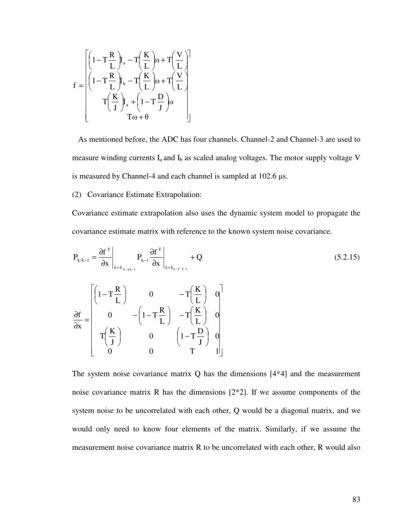
83
��������
�
�
�
+
��
���
� −+��
���
�
��
���
�+��
���
�−��
���
� −
��
���
�+��
���
�−��
���
� −
=
�T�
�JD
T1IJK
T
LV
T�LK
TILR
T1
LV
T�LK
TILR
T1
f
a
b
a
As mentioned before, the ADC has four channels. Channel-2 and Channel-3 are used to
measure winding currents Ia and Ib as scaled analog voltages. The motor supply voltage V
is measured by Channel-4 and each channel is sampled at 102.6 �s.
(2) Covariance Estimate Extrapolation:
Covariance estimate extrapolation also uses the dynamic system model to propagate the
covariance estimate matrix with reference to the known system noise covariance.
Qx
fP
xf
P1k1k1k1k xx
T
1k
xx
T
1kk +∂
∂∂
∂=−−−− =
−=
− (5.2.15)
��������
�
�
�
��
���
� −��
���
�
��
���
�−��
���
� −−
��
���
�−��
���
� −
=∂∂
1T00
0JD
T10JK
T
0LK
TLR
T10
0LK
T0LR
T1
xf
The system noise covariance matrix Q has the dimensions [4*4] and the measurement
noise covariance matrix R has the dimensions [2*2]. If we assume components of the
system noise to be uncorrelated with each other, Q would be a diagonal matrix, and we
would only need to know four elements of the matrix. Similarly, if we assume the
measurement noise covariance matrix R to be uncorrelated with each other, R would also

84
be a diagonal matrix. The winding currents Ia and Ib have the same noise characteristics.
The system and measurement noise covariance matrices will be;
����
�
�
�
=
44
33
11
11
q0000q0000q0000q
Q ��
�
�=
11
11
r00r
R
(3) Kalman filter gain computation:
The Kalman filter gain computation is done by weighting the prior knowledge of the
measurement noise with the state estimate covariance. The actual measurements have no
effect on the gain computation.
1
xx
T
1kkxxxx
T
1kkk Rx
hP
xh
xh
PK1k1k1k1k1k1k
−
=−
==− �
�
�
�
�+
∂∂
∂∂
∂∂=
−−−−−−
(5.2.16)
��
�
�==
b
a
II
Cxh
��
�
�=
∂∂
00100001
xh
(4) State estimate update:
The state estimate update is done by adding the product of the gain matrix and the
measurement residual to the state estimate propagation. The measurement vector is
represented as
( )0,xhy 1-kk =
The state estimation at time k is given as;
))0,x(hy(Kx x 1kkkk1kkk −− −+= (5.2.17)
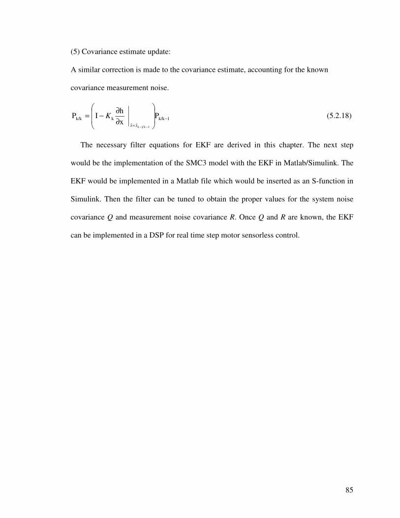
85
(5) Covariance estimate update:
A similar correction is made to the covariance estimate, accounting for the known
covariance measurement noise.
1k/kˆˆ
kk/k Pxh
IP11
−=
��
�
�
��
�
�
∂∂−=
−− kkxx
K (5.2.18)
The necessary filter equations for EKF are derived in this chapter. The next step
would be the implementation of the SMC3 model with the EKF in Matlab/Simulink. The
EKF would be implemented in a Matlab file which would be inserted as an S-function in
Simulink. Then the filter can be tuned to obtain the proper values for the system noise
covariance Q and measurement noise covariance R. Once Q and R are known, the EKF
can be implemented in a DSP for real time step motor sensorless control.

86
CHAPTER VI
CONCLUSIONS AND FUTURE RESEARCH
This thesis makes two primary contributions to the literature. First, it demonstrates how
field oriented control can be used in step motors, and provides experimental results
showing its implementation. With the current emphasis on energy conservation, the
electric drive has to be made more efficient and smoother. The open-loop performance of
step motors is limited due to the lack of control of the torque angle of the step motor,
while field oriented control adjusts the step motor torque angle to achieve maximum
performance of the motor. Field oriented control also eliminates skipped steps and
stepping resonance which is a common problem in stepping control. But it is more
expensive compared to stepping control in terms of circuit components and complexity in
circuit and software design. Driving the step motor using SMC3 drive by stepping mode
requires much less powerful micro-processor and software coding is much simpler as it
does not require complex filed-oriented software routine.
The second contribution of this thesis is that it shows how a Kalman filter can be used
to implement sensorless field oriented control of step motors. As explained earlier, the
sensed winding current is quite noisy and a Kalman filter provides better winding current

86
estimation. Sensorless field oriented control of step motors provides a cost effective and
more reliable system as it uses less physical components than encoder-based systems.
The next step in SMC3 design is to implement sensorless step motor control. The
basic approach on how to implement sensorless step motor control is given in this thesis.
The system noise covariance Q and measurement noise covariance R will be tuned so that
real time step motor sensorless control can be implemented in DSP. Once sensorless
control is implemented, speed control [19] or torque control can be implemented using
various advanced control strategies (optimal control [21], fuzzy logic [22], H� control
[23], etc.).
88
BIBILIOGRAPHY
[1]. Acarnley, P.P., “Stepping Motors: a guide to theory and practice: Fourth
Edition,” Institution of Electrical Engineers, London, 2002.
[2]. ADSP-2100 Family User’s Manual (Third Edition), Analog Devices Inc.,
1995.
[3]. Simon D. and Feucht D.,”DSP-Based Field-Oriented Step Motor Control,”
SHARC International DSP Conference, Boston, pp. 303-309, 2001.
[4]. Microchip Technology Inc., “Stepping Motor Fundamentals,” Literature
Number: AN907.
[5]. Holtz J., “Pulsewidth Modulation for Electric Power Conversion,”
Proceedings of the IEEE, vol.82, No. 8, pp. 1194-1212 August 1994.
[6]. A. Nabae, S.Ogasawara, and H. Akagi, “A Novel Control Scheme for
Current- Controlled PWM Inverters,” IEEE Transactions on Industry
Applications, vol. IA-22, pp. 697-701, July/Aug. 1986.
[7]. Pillay P., and Krishnan R., “Control Characteristics and Speed Controller
Design for a High Performance Permanent Magnet Synchronous Motor
Drive,” IEEE Transactions on Power Electronics, vol.5, No. 2, pp. 151-159,
April 1990.
[8]. Wall, R.W., “Simple Method for Detecting Zero Crossing,” Proceedings of
the 29th Annual Conference of the IEEE Industrial Electronics Society,
Paper#00291.

89
[9]. Microchip Technology Inc., “Motor Control Sensor Feedback Circuit,”
Literature number: AN894.
[10]. Analog Devices, “AD7811 datasheet”.
[11]. Digital Signal Processing Applications Using the ADSP-2100 Family,
Volume 1, Prentice Hall, 1992.
[12]. Nagrath I., and Gopal M., “Control Systems Engineering: Third Edition,”
New Age International Publishers.
[13]. Welch R.H., “Measuring Permanent Magnet DC Motor Parameters- Part II:
Brushless DC Motors,” AIME, Reliance Motion Control, Eden Prairie,
Minnesota.
[14]. Ohm D. and Oleksuk R., “On practical Digital Current Regulator design for
PM Synchronous Motor drives,” IEEE Applied Power Electronics Conference
and Exposition, Vol.1, pp. 56-63, Feb. 1998.
[15]. Texas Instruments, “Digital Signal Processings Solutions for Motor Control
Using the TMS320F240 DSP-Controller,” Literature number: SPRA 345, Sep
1996.
[16]. Obermeier C., Kellermann H., and Brandenburg, G., “Sensorless field
oriented speed control of a hybrid and a permanent magnet disk stepper motor
using an extended Kalman filter,” IEEE International Electrical Machines and
Drives Conference Record, pp. MC3/5.1-MC3/5.3, 1997.
[17]. Kalman, R.E., “A New Approach to Linear Filtering and Prediction
Problems,” Transactions of the ASME--Journal of Basic Engineering, vol.82,
pp. 35-45, 1960.

90
[18]. Stengel R., “Optimal Control and Estimation: First Edition,” Dover
Publication, Inc., New York.
[19]. Behal A., Feemster M., Dawson D., and Mangal A., “Sensorless Rotor
Velocity Tracking Control of the Permanent Magnet Stepper Motor,”
Proceedings of the IEEE International conference on Control Applications,
pp. 150-154, Alaska, September, 2000.
[20]. Simon D., “Design and rule base reduction of a fuzzy filter for the estimation
of motor currents,” International Journal of Approximate Reasoning, 2000,
pp. 145-167.
[21]. Crnosija P., Kuzmanvoic B., and Ajdukovic S., “Microcomputer
implementation of optimal algorithms for closed-loop control of hybrid
stepper motor drives,” IEEE Transactions on Industrial Electronics, vol. 47,
pp. 1319-1325, 2000.
[22]. Qingding G. and Yanna S., “H� control based on internal model theory for
linear permanent magnet synchronous servo motor (LPSM),” Control Theory
& Applications, vol.17, pp. 509-512, 2000.
[23]. Betin F., Pinchon D., and Capolino G., “Fuzzy logic applied to speed control
of a stepping motor drive,” IEEE Transactions on Industrial Electronics, vol.
47, pp.610-622, 2000.

91
Appendix

92
APPENDIX A SOFTWARE LISTING
{**********************************************************************} { SMC3F.DSP } { encoder-based closed loop control } { automatic phase reference alignment on DSP reset } { You can set the variable open_loop=1 to achieve open loop control. } { You can set the variable open_loop=0 to achieve closed loop control } { using the encoder input. } .module/RAM/ABS=0 smc3f; { Assemble-time constants } { ADSP2101 addresses } .const SPORT1_Autobuf = 0x3fef; .const SPORT1_RFSDIV = 0x3ff0; .const SPORT1_SCLKDIV = 0x3ff1; .const SPORT1_Control_Reg = 0x3ff2; .const SPORT0_Autobuf = 0x3ff3; .const SPORT0_RFSDIV = 0x3ff4; .const SPORT0_SCLKDIV = 0x3ff5; .const SPORT0_Control_Reg = 0x3ff6; .const SPORT0_TX_Channels0 = 0x3ff7; .const SPORT0_TX_Channels1 = 0x3ff8; .const SPORT0_RX_Channels0 = 0x3ff9; .const SPORT0_RX_Channels1 = 0x3ffa; .const TSCALE = 0x3ffb; .const TCOUNT = 0x3ffc; .const TPERIOD = 0x3ffd; .const DM_Wait_Reg = 0x3ffe; .const System_Control_Reg = 0x3fff; .const counts_revel = 80; { encoder counts/electrical rev } { 1000 lines/rev, 4000 counts/rev } .const half_counts_revel = counts_revel / 2; .const fourth_counts_revel = counts_revel / 4; { 1/4 rev counts } .const phase_scale = 819; { scale phase: 32768/half_counts_revel } { 32768/40 = 819.2 => 819 } .const via_scale = 2; .const pro_gain = 5; .const ticks = 10000; { manual z-phase advance every "ticks" timer ints } .const timebase = 100; { how often to increment phase for open loop control }

93
{ Port address } .const Encoder_In = 0x0000; { Data variables/buffers } .var/dm/ram open_loop; { flag for open loop control } .init open_loop: 0; .var/dm/ram ax0_reg; { register storage for interrupts } .var/dm/ram ay0_reg; .var/dm/ram ar_reg; .var/dm/ram ay1_reg; .var/dm/ram sr0_reg; .var/dm/ram sr1_reg; .var/dm/ram ADC_Control_reg; .var/dm/ram irq2_tick; { irq2 clock } .init irq2_tick: 0; .var/dm/ram timer_tick; { timer clock for manual z-phase advance } .init timer_tick: 0; .var/dm/ram advance_tick; { open loop control clock } .init advance_tick: 0; .var/dm/ram/circ pwm_buf[2]; { PWMB first, then PWMA } .init pwm_buf: 0x0000, 0x0000; .var/dm/ram tx1_flag; .var/dm/ram/circ adc_buf[4]; { Vspd } .init adc_buf: 900; .var/dm/ram magnitude; { current magnitude of sin/cos in 1.15 format } .init magnitude: 0; .var/dm/ram encoder[2]; { b7-b0: SW1 SW0 VZB VZA /STOP Z B A } { latest value at 0 index } .var/dm/ram encoder_cnt; { signed encoder count } .init encoder_cnt: 0; .var/dm/ram encoder_state[8]; { previous, present: B A } .init encoder_state: 0, -1, 1, 2, 1, 0, 2, -1; .var/dm/ram phase; { el phase, in encoder counts } .init phase: 0; .var/dm/ram Z_phase; { phase offset, in encoder counts } .init Z_phase: 0; .var/dm/ram/circ sin_coeff[5]; { signed; used by sine subroutine }

94
.init sin_coeff: 0x3240, 0x0053, 0xAACC, 0x08B7, 0x1CCE; .var/dm/ram angle; { total angle } .init angle: 0; .var/dm/ram last_int; { when the last encoder count occurred } .init last_int: 0; .var/dm/ram speed_cnt; { speed control counter } .init speed_cnt: 0; .var/dm/ram angle_ref; { speed reference } .init angle_ref: 0; .var/dm/ram omega_ref; { angular velocity reference } .init omega_ref: 0; .const speed_ticks = 100; { speed control every speed_ticks interrupts } .var/dm/ram xhat[2]; .init xhat: 0, 0; .var/dm/ram RevIter1; .init RevIter1: 0; .var/dm/ram RevIter2; .init RevIter2: 0; .var/dm/ram angle1; .init angle1: 0; .var/dm/ram direction; .init direction: 0; .var/dm/ram iteration; .init iteration: 0; .var/dm/ram angle_tot; .init angle_tot: 0; .var/dm/ram via_count; .init via_count: 0; .var/dm/ram via_count1; .init via_count1: 0; .var/dm/ram via_old; .init via_old: 0; .var/dm/ram via_fed; .init via_fed: 0; .var/dm/ram pid_flag; .init pid_flag: 0; .var/dm/ram sign_flag; .init sign_flag: 0; .var/dm/ram abs_err; .init abs_err: 0; .var/dm/ram p_con; .init p_con: 0; .var/dm/ram mag_err; .init mag_err: 0; .var/dm/ram/circ scale_buf[4]; { PWMB first, then PWMA }

95
.init scale_buf: 0,10,0,0; .var/dm/ram/circ co_buf[3]; { PWMB first, then PWMA } .init co_buf: 0x0000, 0x0000,0x0000; { Interrupt vector table } JUMP dsp_reset; RTI; RTI; RTI; { 00: reset } JUMP irq2; RTI; RTI; RTI; { 04: IRQ2 } RTI; RTI; RTI; RTI; { 08: SPORT0 tx } JUMP rx0_int; RTI; RTI; RTI; { 0C: SPORT0 rx } JUMP tx1_int; RTI; RTI; RTI; { 10: SPORT1 tx or IRQ1 } RTI; RTI; RTI; RTI; { 14: SPORT1 rx or IRQ0 } JUMP timer_int; RTI; RTI; RTI; { 18: timer } { DSP intialization } dsp_reset: { DSP register initialization } AX0 = 0x1C1B; DM(System_Control_Reg) = AX0; AX0 = 0x36DB; DM(DM_Wait_Reg) = AX0; { 200 ns } { SPORT0: ADC } AX0 = 0x6A09; { 10 bits/frame } DM(SPORT0_Control_Reg) = AX0; AX0 = 0x0000; DM(SPORT0_Autobuf) = AX0; { no autobuf } { SCLKDIV = CLKOUT/2*SCLK - 1) = 20 MHz/2*1 MHz - 1 = 9 } AX0 = 9; DM(SPORT0_SCLKDIV) = AX0; { SPORT1: PWMs } AX0 = 0x7FC8; DM(SPORT1_Control_Reg) = AX0; { SCLKDIV = CLKOUT/2*SCLK - 1) = 20 MHz/2*1 MHz - 1 = 9 } AX0 = 9; DM(SPORT1_SCLKDIV) = AX0; { Timer period = 10 us }

96
AX0 = 0; DM(TSCALE) = AX0; { DSP clock period = 50 ns } AX0 = 199; DM(TPERIOD) = AX0; { Init positional variables } SR0 = DM(Encoder_In); AY0 = 3; { mask B A track bits } AR = SR0 AND AY0; DM(encoder) = AR; DM(encoder + 1) = AR; { init previous encoder sample } SR = LSHIFT SR0 BY -6 (LO); I0 = ^pwm_buf; L0 = %pwm_buf; M0 = 0; M1 = 1; I5 = ^sin_coeff; L5 = %sin_coeff; I6 = 0; { not dedicated } L6 = 0; { used as table index for encoder_state } I4= ^adc_buf; L4= %adc_buf; I1=^co_buf; L1=%co_buf; I7 = ^scale_buf; L7 = %scale_buf; M4 = 0; M5 = 1; M6 = -1; M7 = 2; { Init. PWM values } DM(I0, M1) = 0; DM(I0, M1) = 0; { Mode register }

97
MSTAT = 0x20; { timer enabled } { Interrupt initialization } ICNTL = 0x07; { edge-sensitive ext. ints., no nesting } IFC = 0x3F; { clear pending interrupts } NOP; { one cycle for ifc write to go into effect } IMASK = 0x2D; { IRQ2, rx0, tx1, timer: 0x2D } { Align z_phase for the maximum speed } call Align; { Go to the main loop } jump main; {*******************************************************************} { Align the phase for maximum speed } Align: call IterTime; { Get the # of control cycles per revolution } AX1 = dm(iteration); dm(RevIter1) = AX1; AY0 = dm(z_phase); { Change the phase alignment } AF = AY0 + 1; AR = AF + 1; dm(z_phase) = AR; call IterTime; { Again get the # of control cycles per revolution } AX1 = dm(iteration); dm(RevIter2) = AX1; AY1 = 1; dm(direction) = AY1; { direction = 1 if we want to increase } AY0 = dm(RevIter1); { z_phase for alignment, -1 if we want } AR = AX1 - AY0; { to decrease z_phase for alignment } if LT jump ReverseDir; { Swap RevIter1 and RevIter2; Set the phase advance direction to -1 } dm(RevIter2) = AY0; dm(RevIter1) = AX1; AY1 = -1; dm(direction) = AY1; ReverseDir: AY0 = dm(RevIter1); AX1 = dm(RevIter2); AR = AX1 - AY0; if GE RTS; dm(RevIter1) = AX1; { RevIter1 = RevIter2 } AR = dm(z_phase); { Advance the phase by +/- 1 } AY1 = dm(direction); AR = AR + AY1;

98
dm(z_phase) = AR; call IterTime; { Wait one iteration for the motor speed } call IterTime; { to settle } AX1 = dm(iteration); dm(RevIter2) = AX1; jump ReverseDir; {*******************************************************************} { The IterTime routine measures how long it takes for one motor revolution } { The number of control cycles required for one motor revolution } { is returned in "iteration". } IterTime: AY0 = 0; dm(iteration) = AY0; { # of control cycles per revolution } dm(angle_tot) = AY0; { total encoder counts measured } AR = AY0 + 1; dm(speed_cnt) = AR; IterWait: call drive; AY0 = dm(speed_cnt); { Wait for a control cycle } AF = pass AY0; if NE jump IterWait; AY0 = dm(iteration); AR = AY0 + 1; { Increment the # of control cycles } dm(iteration) = AR; AY0 = dm(angle1); AX0 = dm(angle_tot); AR = AX0 + AY0; { Increment the # of encoder counts } dm(angle_tot) = AR; AY0 = 4000; { Assume one control cycle / 1 msec } AF = AR - AY0; { 4000 encoder counts per revolution } if GE RTS; { Return after one revolution } AY0 = 2000; { AX1 = 2000 after 2 seconds } AX1 = dm(iteration); AF = AX1 - AY0; { If 2 seconds have passed without a rev } if LT jump IterWait; { then bump the z-phase and start over } AR = dm(z_phase); AY0 = 10; AR = AR + AY0; dm(z_phase) = AR; jump IterTime; {*******************************************************************} { Interrupted loop } main:

99
call drive1; JUMP main; { loop } {*******************************************************************} drive: { ADC0 (vspd) input scaling } AX0 = DM(adc_buf); AY0 = 521; { fs/2 offset of vspd 10-bit ADC input } ENA AR_SAT; { no 2's complement wraparound } AR = AX0 - AY0; { signed voltage offset } SR = ASHIFT AR BY 6 (LO) ; { 1.15 format fraction } AR = ABS SR0; { Limit max magnitude to 0x7F00 = 254 * 2^7 } AY0 = 0x7F00; { +fs magnitude = 7F00 } AF = AR - AY0; IF GT AR = PASS AY0; AF = PASS SR0; IF NEG AR = -AR; { AR = scaled command input } AR = 0x7F00; DM(magnitude) = AR; DIS AR_SAT; CALL phase_generator; rts; {*******************************************************************} drive1: AX0=DM(adc_buf); AY0=DM(adc_buf+1); AR=AX0-AY0; {error} MX0=DM(I1,M1),MY0=PM(I7,M5); MR=MX0*MY0(SS),MX1=DM(I1,M1),MY0=PM(I7,M5); MR=MR+MX1*MY0(SS),MY0=PM(I7,M5); {pid controller} MR=MR+AR*MY0(SS),MX0=DM(I1,M1),MY0=PM(I7,M5); MR=MR+MX0*MY0(RND),DM(I1,M1)=MX1; SR=ASHIFT MR1(HI),DM(I1,M1)=AR; DM(I1,M1)=SR1; AX0=SR1; AY0 = 521; { fs/2 offset of vspd 10-bit ADC input } ENA AR_SAT; { no 2's complement wraparound } AR = AX0 - AY0; { signed voltage offset } SR = ASHIFT AR BY 6 (LO) ; { 1.15 format fraction } AR = ABS SR0; { Limit max magnitude to 0x7F00 = 254 * 2^7 } AY0 = 0x7F00; { +fs magnitude = 7F00 }

100
AF = AR - AY0; IF GT AR = PASS AY0; AF = PASS SR0; IF NEG AR = -AR; { AR = scaled command input } DM(magnitude) = AR; DIS AR_SAT; phase_gen: CALL phase_generator; rts; {*******************************************************************} phase_generator: { Get the total phase by adding phase + z-phase } AX0 = DM(phase); AY0 = DM(Z_phase); AR = AX0 + AY0; { Put the total phase between +/- 40 } AX1 = AR; call CheckPhaseWrap; { scale the phase for the sine function } MY1 = phase_scale; { phase_scale = 32768/40 = 819.2 => 819 } ENA M_MODE; { integer mpy } MR = AR * MY1 (SS); { vector generator - sin/cos synthesis } AY1 = MR0; { save arg for cos } AR = MR0; DIS M_MODE; { fractional mpy } CALL sine; { sin => A } MX0 = AR; AX0 = 0x4000; { 90 deg } AR = AX0 - AY1; { cos(theta) = sin(pi/2 - theta) } CALL sine; { cos => B } { AR => PWMB; MX0 => PWMA } { PWM format: 1 sign bit (hi = +), 8 bits magnitude } AY0 = 0x100; { bit 9 positive sign bit } MY0 = DM(magnitude); { PWMB } MR = AR * MY0 (SU); SR = ASHIFT MR1 BY -7 (LO); { PWM = 9 MSBs } AR = ABS SR0; { magnitude }

101
IF POS AR = AR OR AY0; { + sign for positive PWM value } DM(pwm_buf) = AR; { update PWMB value } MR = MX0 * MY0 (SU); { PWMA } SR = ASHIFT MR1 BY -7 (LO); AR = ABS SR0; { magnitude } IF POS AR = AR OR AY0; { + sign for positive PWM value } DM(pwm_buf + 1) = AR; { update PWMA value } RTS; {*******************************************************************} sine: { 1.15 format: AR = arg (-180 deg = 0x8000 to +180 deg = 0x7FFF), AR = sin; uses: AY0, AF, AR, MX1, MY1, MF, MR, SR, I5, M5 25 cycles } AY0 = 0x4000; AX0 = AR; AF = AX0 AND AY0; { Check 2nd or 4th quad. } IF NE AR = -AX0; AY0 = 0x7FFF; AR = AR AND AY0; { remove sign bit } MY1 = AR; MF = AR * MY1 (RND), MX1 = DM(I5, M5); { MF = x^2 } MR = MX1 * MY1 (SS), MX1 = DM(I5, M5); { MR = c1*x } CNTR = 3; DO sine1 UNTIL CE; MR = MR + MX1 * MF (SS); sine1: MF = AR * MF (RND), MX1 = DM(I5, M5); MR = MR + MX1 * MF (SS); SR = ASHIFT MR1 BY 3 (HI); SR = SR OR LSHIFT MR0 BY 3 (LO); { convert to 1.15 format } AR = PASS SR1; IF LT AR = PASS AY0; { saturate if needed } AF = PASS AX0; IF LT AR = -AR; { negate output if needed } RTS; {*******************************************************************} { irq2: external PWM counter overflow => irq2 ADC & PWM driver: 25.6 us - every tick } irq2: DM(ax0_reg) = AX0; { save registers used in irq2 } DM(ay0_reg) = AY0; DM(ay1_reg)= AY1;

102
DM(ar_reg) = AR; DM(sr0_reg)=SR0; DM(sr1_reg)=SR1; { PWM Driver } AX0 = DM(pwm_buf); TX1 = AX0; { start tx of PWMB } AX0 = 0xFFFF; DM(tx1_flag) = AX0; AY0= DM(ADC_Control_Reg); AY1= ^adc_buf; AX0= I4; AR= AX0-AY1; SR=LSHIFT AR BY 2(LO); AR= SR0 OR AY0; TX0 =AR; AX0 = DM(ax0_reg); { restore used registers in irq2 } AY0 = DM(ay0_reg); AR = DM(ar_reg); AY1=DM(ay1_reg); SR0=DM(sr0_reg); SR1=DM(sr1_reg); RTI; {*******************************************************************} { Timer Interrupt Routine: Encoder driver; switch debounce: 10 ms } timer_int: ENA SEC_REG; { Check if we should use open loop or closed loop control } AR = dm(open_loop); AR = pass AR; if EQ call ClosedLoopControl; AR = dm(open_loop); AR = pass AR; if NE call OpenLoopControl; { Make sure phase is in the +/- 40 range } AX1 = dm(phase); call CheckPhaseWrap; dm(phase) = AR; { Check if the user wants to adjust the z-phase } call AdjustZPhase; { Call the speed control routine } call speed_control; RTI;

103
{*******************************************************************} AdjustZPhase: { manual phase advance tick counter } AY0 = DM(timer_tick); AR = AY0 + 1; AX0 = ticks; AF = AX0 - AY0; IF LE AR = PASS 0; DM(timer_tick) = AR; IF NE rts; { check for z phase adjustment if timer_tick = ticks } { Adjust Z_phase } AY1 = DM(Z_phase); AF = PASS AY1; AX0 = DM(Encoder_In); AY0 = 0x0040; { CNFG1 bit - active low } AR = AX0 AND AY0; IF EQ AF = AF + 1; AR = PASS AF; DM(Z_phase) = AR; rts; {*******************************************************************} ClosedLoopControl: { encoder driver } SR0 = DM(encoder); DM(encoder + 1) = SR0; { advance previous encoder sample } SR = LSHIFT SR0 BY 2 (LO); { shift previous sample by 2 } MR0 = DM(Encoder_In); { SR = LSHIFT MR0 BY -4 (HI); SR1 = MR0; } AY1 = 3; AR = MR0 AND AY1; { A B tracks only } DM(encoder) = AR; { store present sample } AY0 = SR0; AR = AR OR AY0; { table index: previous B A, present B A } AY0 = 8; AF = AR - AY0; IF GE AR = NOT AR; { if GE 8, invert bits } AY0 = 7; AR = AR AND AY0; { 3-bit index } AY0 = ^encoder_state; AR = AR + AY0; { add table base address }
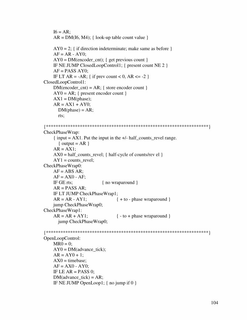
104
I6 = AR; AR = DM(I6, M4); { look-up table count value } AY0 = 2; { if direction indeterminate; make same as before } AF = AR - AY0; AY0 = DM(encoder_cnt); { get previous count } IF NE JUMP ClosedLoopControl1; { present count NE 2 } AF = PASS AY0; IF LT AR = -AR; { if prev count < 0, AR <= -2 } ClosedLoopControl1: DM(encoder_cnt) = AR; { store encoder count } AY0 = AR; { present encoder count } AX1 = DM(phase); AR = AX1 + AY0; DM(phase) = AR; rts; {*******************************************************************} CheckPhaseWrap: { input = AX1. Put the input in the +/- half_counts_revel range. { output = AR } AR = AX1; AX0 = half_counts_revel; { half-cycle of counts/rev el } AY1 = counts_revel; CheckPhaseWrap0: AF = ABS AR; AF = AX0 - AF; IF GE rts; { no wraparound } AR = PASS AR; IF LT JUMP CheckPhaseWrap1; AR = AR - AY1; { + to - phase wraparound } jump CheckPhaseWrap0; CheckPhaseWrap1: AR = AR + AY1; { - to + phase wraparound } jump CheckPhaseWrap0; {*******************************************************************} OpenLoopControl: MR0 = 0; AY0 = DM(advance_tick); AR = AY0 + 1; AX0 = timebase; AF = AX0 - AY0; IF LE AR = PASS 0; DM(advance_tick) = AR; IF NE JUMP OpenLoop1; { no jump if 0 }

105
MR0 = 1; { Open-loop advance of phase by incrementing at timebase rate } OpenLoop1: AY0 = MR0; { = 1 on timebase timeout } { iterate phase: AY0 = phase increment } AX1 = DM(phase); AR = AX1 + AY0; DM(phase) = AR; { advance the phase } rts; {*******************************************************************} speed_control: { Speed control } AR = DM(encoder_cnt); { get the encoder count } AY0 = DM(angle); AR = AR + AY0; DM(angle) = AR; { total angle } AY0 = DM(speed_cnt); { filtering and } AF = AY0 + 1; { speed control every speed_ticks ints } AR = PASS AF; AX0 = speed_ticks; AF = AX0 - AF; if EQ AR = PASS 0; DM(speed_cnt) = AR; if NE RTS; MR0 = DM(angle); { Save the total angle in MR0 and angle1 } AR = ABS MR0; DM(angle1) = AR; MR0 = AR; AX0 = 0; { reset the total angle to 0 } DM(angle) = AX0; RTS; {*******************************************************************} { Turn off autobuffering at pwm_buf rollover } tx1_int: DM(ax0_reg) = AX0; { Save regs } DM(ar_reg) = AR; AX0 = DM(tx1_flag); AR = PASS AX0; IF EQ JUMP tx1_int1;

106
AX0 = DM(pwm_buf + 1); { PWMA } TX1 = AX0; AX0 = 0; DM(tx1_flag) = AX0; tx1_int1: AX0 = DM(ax0_reg); { retsore regs } AR = DM(ar_reg); RTI; {*******************************************************************} rx0_int: { Acquire ADC data into adc_buf } DM(ax0_reg) = AX0; { save reg } AX0 = RX0; { prev ADC sample in } MODIFY (I4,M6); DM(I4,M7)=AX0; AX0 = DM(ax0_reg); RTI; .endmod; {****************************** end ********************************}