Embed Size (px)
Citation preview

Feature-based Similarity Search in Graph
Structures
Xifeng Yan
University of Illinois at Urbana-Champaign
Feida Zhu
University of Illinois at Urbana-Champaign
Philip S. Yu
IBM T. J. Watson Research Center
and
Jiawei Han
University of Illinois at Urbana-Champaign
Similarity search of complex structures is an important operation in graph-relatedapplications since exact matching is often too restrictive. In this article, we inves-tigate the issues of substructure similarity search using indexed features in graphdatabases. By transforming the edge relaxation ratio of a query graph into themaximum allowed feature misses, our structural filtering algorithm can filter graphswithout performing pairwise similarity computation. It is further shown that us-ing either too few or too many features can result in poor filtering performance.Thus the challenge is to design an effective feature set selection strategy that couldmaximize the filtering capability. We prove that the complexity of optimal featureset selection is Ω(2m) in the worst case, where m is the number of features forselection. In practice, we identify several criteria to build effective feature sets forfiltering, and demonstrate that combining features with similar size and selectivitycan improve the filtering and search performance significantly within a multi-filtercomposition framework. The proposed feature-based filtering concept can be gener-alized and applied to searching approximate non-consecutive sequences, trees, andother structured data as well.
Categories and Subject Descriptors: H.2.4 [Database Management]: Systems – Query process-
This is a preliminary release of an article accepted by ACM Transactions on Database Systems.The definitive version is currently in production at ACM and, when released, will supersede this
version.Authors’ address: X. Yan, F. Zhu, Department of Computer Science, University of Illinois at
Urbana-Champaign, Urbana, IL 61801, Email: xyan, [email protected]; P. S. Yu, IBM T. J.Watson Research Center, Hawthorne, NY 10532, Email: [email protected]; J. Han, Departmentof Computer Science, University of Illinois at Urbana-Champaign, Urbana, IL 61801, Email:
[email protected] to make digital/hard copy of all or part of this material without fee for personal
or classroom use provided that the copies are not made or distributed for profit or commercialadvantage, the ACM copyright/server notice, the title of the publication, and its date appear, andnotice is given that copying is by permission of the ACM, Inc. To copy otherwise, to republish, to
post on servers, or to redistribute to lists requires prior specific permission and/or a fee. Requestpermissions from Publications Dept, ACM Inc., fax +1 (212) 869-0481, or [email protected]© 2006 ACM 0362-5915/2006/0300-0001 $5.00
ACM Transactions on Database Systems, Vol. V, No. N, June 2006, Pages 1–0??.
2 · Xifeng Yan et al.
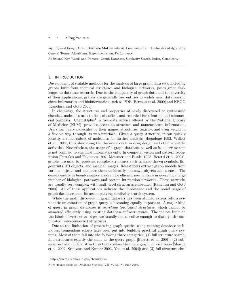
ing, Physical Design; G.2.1 [Discrete Mathematics]: Combinatorics – Combinatorial algorithms
General Terms: Algorithms, Experimentation, Performance
Additional Key Words and Phrases: Graph Database, Similarity Search, Index, Complexity
1. INTRODUCTION
Development of scalable methods for the analysis of large graph data sets, includinggraphs built from chemical structures and biological networks, poses great chal-lenges to database research. Due to the complexity of graph data and the diversityof their applications, graphs are generally key entities in widely used databases inchem-informatics and bioinformatics, such as PDB [Berman et al. 2000] and KEGG[Kanehisa and Goto 2000].
In chemistry, the structures and properties of newly discovered or synthesizedchemical molecules are studied, classified, and recorded for scientific and commer-cial purposes. ChemIDplus1, a free data service offered by the National Libraryof Medicine (NLM), provides access to structure and nomenclature information.Users can query molecules by their names, structures, toxicity, and even weight ina flexible way through its web interface. Given a query structure, it can quicklyidentify a small subset of molecules for further analysis [Hagadone 1992, Willettet al. 1998], thus shortening the discovery cycle in drug design and other scientificactivities. Nevertheless, the usage of a graph database as well as its query systemis not confined to chemical informatics only. In computer vision and pattern recog-nition [Petrakis and Faloutsos 1997, Messmer and Bunke 1998, Beretti et al. 2001],graphs are used to represent complex structures such as hand-drawn symbols, fin-gerprints, 3D objects, and medical images. Researchers extract graph models fromvarious objects and compare them to identify unknown objects and scenes. Thedevelopments in bioinformatics also call for efficient mechanisms in querying a largenumber of biological pathways and protein interaction networks. These networksare usually very complex with multi-level structures embedded [Kanehisa and Goto2000]. All of these applications indicate the importance and the broad usage ofgraph databases and its accompanying similarity search system.
While the motif discovery in graph datasets has been studied extensively, a sys-tematic examination of graph query is becoming equally important. A major kindof query in graph databases is searching topological structures, which cannot beanswered efficiently using existing database infrastructures. The indices built onthe labels of vertices or edges are usually not selective enough to distinguish com-plicated, interconnected structures.
Due to the limitation of processing graph queries using existing database tech-niques, tremendous efforts have been put into building practical graph query sys-tems. Most of them fall into the following three categories: (1) full structure search:find structures exactly the same as the query graph [Beretti et al. 2001]; (2) sub-structure search: find structures that contain the query graph, or vice versa [Shashaet al. 2002, Srinivasa and Kumar 2003, Yan et al. 2004]; and (3) full structure sim-
1http://chem.sis.nlm.nih.gov/chemidplus.
ACM Transactions on Database Systems, Vol. V, No. N, June 2006.

Feature-based Similarity Search in Graph Structures · 3
ilarity search: find structures that are similar to the query graph [Petrakis andFaloutsos 1997, Willett et al. 1998, Raymond et al. 2002]. These kinds of queriesare very useful. For example, in substructure search, a user may not know theexact composition of the full structure he wants, but requires that it contain a setof small functional fragments.
A common problem in substructure search is: what if there is no match or veryfew matches for a given query graph? In this situation, a subsequent query refine-ment process has to be taken in order to find the structures of interest. Unfortu-nately, it is often too time-consuming for a user to perform manual refinements.One solution is to ask the system to find graphs that nearly contain the entirequery graph. This similarity search strategy is more appealing since the user canfirst define the portion of the query for exact matching and let the system changethe remaining portion slightly. The query could be relaxed progressively until arelaxation threshold is reached or a reasonable number of matches are found.
N
N
N
N
O
O
(a) caffeine
N
N
N
N
O
O
(b) thesal
N
NS
O O
N
NN
N
O
O
(c) viagra
Fig. 1. A Chemical Database
N
N
N
N
O
Fig. 2. A Query Graph
Example 1. Figure 1 is a chemical dataset with three molecules. Figure 2 showsa substructure query. Obviously, no match exists for this query graph. If we relaxthe query with one edge miss, caffeine and thesal in Figures 1(a) and 1(b) will begood matches. If we relax the query further, the structure in Figure 1(c) could alsobe an answer.
Unfortunately, few systems are available for this kind of search scheme in largescale graph databases. Existing tools such as ChemIDplus only provide the fullstructure similarity search and the exact substructure search. Other studies usuallyfocus on how to compute the substructure similarity between two graphs efficiently[Nilsson 1980]. This leads to the linear complexity with respect to the size of graphdatabase since each graph in the database has to be checked.
ACM Transactions on Database Systems, Vol. V, No. N, June 2006.

4 · Xifeng Yan et al.
Given that the pairwise substructure similarity computation is very expensive,practically it is not affordable in a large database. A naıve solution is to forma set of subgraph queries with one or more edge misses and then use the exactsubstructure search. This does not work well even when the number of misses isslightly higher than 1. For example, if we allow three edges to be missed in a 20-edge query graph, it may generate
(
203
)
= 1, 140 substructure queries, which is tooexpensive to check. Therefore, a better solution is greatly preferred.
In this article, we propose a feature-based structural filtering algorithm, calledGrafil (Graph Similarity Filtering), to perform substructure similarity search ina large scale graph database. Grafil models each query graph as a set of featuresand transforms edge misses into feature misses in the query graph. With an up-per bound on the maximum allowed feature misses, Grafil can filter many graphsdirectly without performing pairwise similarity computations. As a filtering tech-nology, Grafil will improve the performance of existing pairwise substructure simi-larity search systems as well as the naıve approach discussed above in large graphdatabases.
To facilitate the feature-based filtering, we introduce two data structures, feature-graph matrix and edge-feature matrix. The feature-graph matrix, initially proposedby Giugno and Shasha [Giugno and Shasha 2002, Shasha et al. 2002], is an indexstructure to compute the difference in the number of features between a query graphand graphs in the database. The edge-feature matrix is built on the fly to computea bound on the maximum allowed feature misses based on a query relaxation ratio.
It will be shown here that using too many features will not improve the filter-ing performance due to a frequency conjugation phenomenon identified through ourstudy. This counterintuitive result inspires us to identify better combinations of fea-tures for filtering purposes. A geometric interpretation is thus proposed to capturethe rationale behind the frequency conjugation phenomenon, which also deepensour understanding of the complexity of optimal feature set selection. We prove thatit takes Ω(2m) steps to find an optimal solution in the worst case, where m is thenumber of features for selection. Practically, we develop a multi-filter compositionstrategy, where each filter uses a distinct and complementary subset of the features.The filters are constructed by a hierarchical, one-dimensional clustering algorithmthat groups features with similar selectivity into a feature set. The experimentalresult shows that the multi-filter strategy can improve performance significantlyfor a moderate relaxation ratio. To the best of our knowledge, there is no previouswork using feature clustering to improve the filtering performance.
A significant contribution of this study is an examination of an increasingly im-portant search problem in graph databases and a new perspective into handling thegraph similarity search: instead of indexing approximate substructures, we proposea feature-based indexing and filtering framework, which is a general model that canbe applied to searching approximate, non-consecutive sequences, trees, and othercomplicated structures as well.
The rest of the article is organized as follows. Related work is presented in Section2. Section 3 defines the preliminary concepts. We introduce our structural filteringtechnique in Section 4, followed by an exploration of optimal feature set selection,its complexity and the development of clustering-based feature selection in Section
ACM Transactions on Database Systems, Vol. V, No. N, June 2006.

Feature-based Similarity Search in Graph Structures · 5
5. Section 6 describes the algorithm implementation, while our performance studyis reported in Section 7. Section 8 concludes our study.
2. RELATED WORK
Structure similarity search has been studied in various fields. Willett et al. [Willettet al. 1998] summarized the techniques of fingerprint-based and graph-based sim-ilarity search in chemical compound databases. Raymond et al. [Raymond et al.2002] proposed a three-tier algorithm for full structure similarity search. Recently,substructure search has attracted lots of attention in the database research com-munity. Shasha et al. [Shasha et al. 2002] developed a path-based approach forsubstructure search, while Srinivasa et al. [Srinivasa and Kumar 2003] built mul-tiple abstract graphs for the indexing purpose. Yan et al. [Yan et al. 2004] tookthe discriminative frequent structures as indexing features to improve the searchperformance.
As to substructure similarity search, in addition to graph edit distance and align-ment distance, maximum common subgraph is used to measure the similarity be-tween two structures. Unfortunately, finding the maximum common subgraph isNP-complete [Garey and Johnson 1979]. Nilsson[Nilsson 1980] presented an al-gorithm for the pairwise approximate substructure matching. The matching isgreedily performed to minimize a distance function for two structures. Hagadone[Hagadone 1992] recognized the importance of substructure similarity search in alarge set of graphs. He used the atom and edge label to do screening. Holder etal. [Holder et al. 1994] adopted the principle of minimum description length for ap-proximate graph matching. Messmer and Bunke [Messmer and Bunke 1998] studiedthe reverse substructure similarity search problem in computer vision and patternrecognition. These methods did not explore the potential of using more compli-cated structures to improve the filtering performance, which is studied extensivelyby our work. In [Shasha et al. 2002], Shasha et al. also extended their substructuresearch algorithm to support queries with wildcards, i.e., don’t care nodes and edges.Different from their similarity model, we do not fix the positions of wildcards, thusallowing a general and flexible search scheme.
In our recent work [Yan et al. 2005], we introduced the basic concept of a feature-based indexing and filtering methodology for substructure similarity search. It wasshown that using either too few or too many features can result in poor filteringperformance. In this extended work, we provide a geometric interpretation to thisphenomena, followed by a rigorous analysis on the feature set selection problemusing a linear inequality system. We propose three optimization problems in ourfiltering framework and prove that each of them takes Ω(2m) steps to find theoptimal solution in the worst case, where m is the number of features for selec-tion. These results ask for selection heuristics, such as clustering-based feature setselection developed in our solution.
Besides the full-scale graph search problem, researchers also studied the approx-imate tree search problem. Wang et al. [Wang et al. 1994] designed an interactivesystem that allows a user to search inexact matchings of trees. Kailing et al. [Kail-ing et al. 2004] presented new filtering methods based on tree height, node degreeand label information.
ACM Transactions on Database Systems, Vol. V, No. N, June 2006.

6 · Xifeng Yan et al.
The structural filtering approach presented in this study is also related to stringfiltering algorithms. A comprehensive survey on various approximate string filter-ing methods was presented by Navarro [Navarro 2001]. The well-known q-grammethod was initially developed by Ullmann [Ullmann 1977]. Ukkonen [Ukkonen1992] independently discovered the q-gram approach, which was further extendedin [Gravano et al. 2001] against large scale sequence databases. These q-gram al-gorithms work for consecutive sequences, not structures. Our work generalized theq-gram method to fit structural patterns of various sizes.
3. PRELIMINARY CONCEPTS
Graphs are widely used to represent complex structures that are difficult to model.In a labeled graph, vertices and edges are associated with attributes, called labels.The labels could be tags in XML documents, atoms and bonds in chemical com-pounds, genes in biological networks, and object descriptors in images. The choiceof using labeled graphs or unlabeled graphs depends on the application need. Thefiltering algorithm we proposed in this article can handle both types efficiently.
Let V (G) denote the vertex set of a graph G and E(G) the edge set. A labelfunction, l, maps a vertex or an edge to a label. The size of a graph is defined bythe number of edges it has, written as |G|. A graph G is a subgraph of G′ if thereexists a subgraph isomorphism from G to G′, denoted by G ⊆ G′, in which case itis called a supergraph of G.
Definition 1 Subgraph Isomorphism. A subgraph isomorphism is an injec-tive function f : V (G) → V (G′), such that (1) ∀u ∈ V (G), f(u) ∈ V (G′) andl(u) = l′(f(u)), and (2) ∀(u, v) ∈ E(G), (f(u), f(v)) ∈ E(G′) and l(u, v) =l′(f(u), f(v)), where l and l′ is the label function of G and G′, respectively. Such afunction f is called an embedding of G in G′.
Given a graph database and a query graph, we may not find a graph (or mayfind only a few graphs) in the database that contains the whole query graph. Thus,it would be interesting to find graphs that contain the query graph approximately,which is a substructure similarity search problem. Based on our observation, thisproblem has two scenarios, similarity search and reverse similarity search.
Definition 2 Substructure Similarity Search. Given a graph databaseD = G1, G2, . . . , Gn and a query graph Q, similarity search is to discover all thegraphs that approximately contain this query graph. Reverse similarity search is todiscover all the graphs that are approximately contained in this query graph.
Each type of search scenario has its own applications. In chemical informatics,similarity search is more popular, while reverse similarity search has key appli-cations in pattern recognition. In this article, we develop a structural filteringalgorithm for similarity search. Nevertheless, our algorithm can also be applied toreverse similarity search with slight modifications.
To distinguish a query graph from the graphs in a database, we call the lattertarget graphs. The question is how to measure the substructure similarity betweena target graph and the query graph. There are several similarity measures. We canclassify them into three categories: (1) physical property-based, e.g., toxicity andweight; (2) feature-based; and (3) structure-based. For the feature-based measure,
ACM Transactions on Database Systems, Vol. V, No. N, June 2006.

Feature-based Similarity Search in Graph Structures · 7
domain-specific elementary structures are first extracted as features. Whether twographs are similar is determined by the number of common features they have.For example, we can compare two compounds based on the number of benzenerings they have. Under this similarity definition, each graph is represented as afeature vector, x = [x1, x2, . . . , xn]T , where xi is the frequency of feature fi. Thedistance between two graphs is measured by the distance between their featurevectors. Because of its efficiency, the feature-based similarity search has becomea standard retrieval mechanism [Willett et al. 1998]. However, the feature-basedapproach only provides a very rough measure on structure similarity since it losesthe global structural connectivity. Sometimes it is hard to build an “elementarystructure” dictionary for a graph database, due to the lack of domain knowledge.
In contrast, the structure-based similarity measure directly compares the topol-ogy of two graphs, which is often costly to compute. However, since this measuretakes structure connectivity fully into consideration, it is more accurate than thefeature-based measure. Bunke and Shearer [Bunke and Shearer 1998] used themaximum common subgraph to measure full structure similarity. Researchersalso developed the concept of graph edit distance by simulating the graph match-ing process in a way similar to the string matching process (akin to string editdistance). No matter what the definition is, the matching of two graphs can beregarded as a result of three edit operations: insertion, deletion, and relabeling.According to the substructure similarity search, each of these operations relaxesthe query graph by removing or relabeling one edge (insertion does not change thequery graph). Thus, we take the percentage of retained edges in the query graph asa similarity measure.
Definition 3 Relaxation Ratio. Given two graphs G and Q, if P is the max-imum common subgraph2 of G and Q, then the substructure similarity between G
and Q is defined by |E(P )||E(Q)| , and 1 − |E(P )|
|E(Q)| is called relaxation ratio.
Example 2. Consider the target graph in Figure 1(a) and the query graph inFigure 2. Their maximum common subgraph has 11 out of the 12 edges. Thus, thesubstructure similarity between these two graphs is around 92% with respect to thequery graph. That also means if we relax the query graph by 8%, the relaxed querygraph is contained in Figure 1(a). The similarity of graphs in Figures 1(b) and1(c) with the query graph is 92% and 67%, respectively.
With the advance of computational power, it is affordable to compute the maxi-mum common subgraph for two sparse graphs. Nevertheless, the pairwise similaritycomputation through a large graph database is still time-consuming. In this article,we want to examine how to build a connection between the structure-based mea-sure and the feature-based measure so that we can use the feature-based measure toscreen the database before performing expensive pairwise structure-based similaritycomputation. Using this strategy, we are able to take advantage of both measures:efficiency from the feature-based measure and accuracy from the structure-basedmeasure.
2The maximum common subgraph is not necessarily connected.
ACM Transactions on Database Systems, Vol. V, No. N, June 2006.
8 · Xifeng Yan et al.
4. STRUCTURAL FILTERING
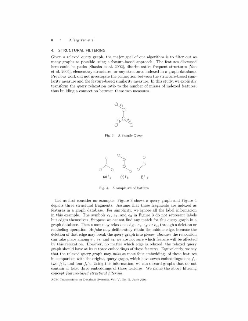
Given a relaxed query graph, the major goal of our algorithm is to filter out asmany graphs as possible using a feature-based approach. The features discussedhere could be paths [Shasha et al. 2002], discriminative frequent structures [Yanet al. 2004], elementary structures, or any structures indexed in a graph database.Previous work did not investigate the connection between the structure-based simi-larity measure and the feature-based similarity measure. In this study, we explicitlytransform the query relaxation ratio to the number of misses of indexed features,thus building a connection between these two measures.
e 1
e 2 e 3
Fig. 3. A Sample Query
(a) f a (b) f b ( c ) f c
Fig. 4. A sample set of features
Let us first consider an example. Figure 3 shows a query graph and Figure 4depicts three structural fragments. Assume that these fragments are indexed asfeatures in a graph database. For simplicity, we ignore all the label informationin this example. The symbols e1, e2, and e3 in Figure 3 do not represent labelsbut edges themselves. Suppose we cannot find any match for this query graph in agraph database. Then a user may relax one edge, e1, e2, or e3, through a deletion orrelabeling operation. He/she may deliberately retain the middle edge, because thedeletion of that edge may break the query graph into pieces. Because the relaxationcan take place among e1, e2, and e3, we are not sure which feature will be affectedby this relaxation. However, no matter which edge is relaxed, the relaxed querygraph should have at least three embeddings of these features. Equivalently, we saythat the relaxed query graph may miss at most four embeddings of these featuresin comparison with the original query graph, which have seven embeddings: one fa,two fb’s, and four fc’s. Using this information, we can discard graphs that do notcontain at least three embeddings of these features. We name the above filteringconcept feature-based structural filtering.
ACM Transactions on Database Systems, Vol. V, No. N, June 2006.

Feature-based Similarity Search in Graph Structures · 9
4.1 Feature-Graph Matrix Index
In order to facilitate the feature-based filtering, we need an index structure, referredto as the feature-graph matrix [Giugno and Shasha 2002, Shasha et al. 2002]. Eachcolumn of the feature-graph matrix corresponds to a target graph in the graphdatabase, while each row corresponds to a feature being indexed. Each entry recordsthe number of the embeddings of a specific feature in a target graph. Suppose wehave a sample database with four graphs, G1, G2, G3, and G4. Figure 5 shows anexample. For instance, G1 has two embeddings of fc. The feature-graph matrixindex is easily maintainable: as each time a new graph is added to the graphdatabase, only an additional column needs to be added.
G 1 G 2 G 3 G 4
f a 0 1 0 0
f b 0 0 1 0
f c 2 3 4 4
Fig. 5. Feature-Graph Matrix Index
Using the feature-graph matrix, we can apply the feature-based filtering on anyquery graph against a target graph in the database using any subset of the indexedfeatures. Consider the query shown in Figure 3 with one edge relaxation. Accordingto the feature-graph matrix in Figure 5, even if we do not know the structure ofG1, we can filter G1 immediately based on the features included in G1, since G1
only has two of all the embeddings of fa, fb, and fc. This feature-based filteringprocess is not involved with any costly structure similarity checking. The onlycomputation needed is to retrieve the features from the indices that belong to aquery graph and compute the possible feature misses for a relaxation ratio. Sinceour filtering algorithm is fully built on the feature-graph matrix index, we need notaccess the physical database unless we want to calculate the accurate substructuresimilarity.
We implement the feature-graph matrix based on a list, where each element pointsto an array representing the row of the matrix. Using this implementation, we canflexibly insert and delete features without rebuilding the whole index. In the nextsubsection, we will present the general framework of processing similarity search,and illustrate the position of our structural filtering algorithm in this framework.
4.2 A General Framework
Given a graph database and a query graph, the substructure similarity search canbe performed within a general framework detailed in the following four steps.
(1) Index construction: Select small structures as features in the graph database,and build the feature-graph matrix between the features and the graphs in thedatabase.
ACM Transactions on Database Systems, Vol. V, No. N, June 2006.

10 · Xifeng Yan et al.
(2) Feature miss estimation: Determine the indexed features belonging to thequery graph, select a feature set (i.e., a subset of the features), calculate thenumber of selected features contained in the query graph and then computethe upper bound of feature misses if the query graph is relaxed with one edgedeletion or relabeling. This upper bound is written as dmax. Some portionof the query graph can be specified as not to be altered, e.g., key functionalstructures.
(3) Query processing: Use the feature-graph matrix to calculate the differencein the number of features between each graph G in the database and query Q.If the difference is greater than dmax, discard graph G. The remaining graphsconstitute a candidate answer set, written as CQ. We then calculate substruc-ture similarity using the existing algorithms and prune the false positives inCQ.
(4) Query relaxation: Relax the query further if the user needs more matchesthan those returned from the previous step; iterate Steps 2 to 4.
The feature-graph matrix in Step 1 is built beforehand and can be used by anyquery. The similarity search for a query graph takes place in Step 2 and Step 3.The filtering algorithm proposed should return a candidate answer set as small aspossible since the cost of the accurate similarity computation is proportional tothe size of the candidate set. Quite a lot of work has been done at calculatingthe pairwise substructure similarity. Readers are referred to the related work in[Nilsson 1980, Hagadone 1992, Raymond et al. 2002].
In the step of feature miss estimation, we calculate the number of features in thequery graph. One feature may have multiple embeddings in a graph; thus, we usethe number of embeddings of a feature as a more precise term. In this article, thesetwo terms are used interchangeably for convenience.
In the rest of this section, we will introduce how to estimate feature misses bytranslating it into the maximum coverage problem. The estimation is further refinedthrough a branch-and-bound method. In Section 5, we will explore the opportunityof using different feature sets to improve filtering efficiency.
4.3 Feature Miss Estimation
Substructure similarity search is akin to approximate string matching. In approx-imate string matching, filtering algorithms such as q-gram achieve the best per-formance because they do not inspect all the string characters. However, filteringalgorithms only work for a moderate relaxation ratio and need a validation algo-rithm to check the actual matches [Navarro 2001]. Similar arguments also applyto our structural filtering algorithm in substructure similarity search. Fortunately,since we are doing substructure search instead of full structure similarity search,usually the relaxation ratio is not very high in our problem setting.
A string with q characters is called a q-gram. A typical q-gram filtering algorithmbuilds an index for all q-grams in a string database. A query string Q is brokeninto a set of q-grams, which are compared against the q-grams of each target stringin the database. If the difference in the number of q-grams is greater than thefollowing threshold, Q will not match this string within k edit distance.
Given two strings P and Q, if their edit distance is k, their difference in the
ACM Transactions on Database Systems, Vol. V, No. N, June 2006.

Feature-based Similarity Search in Graph Structures · 11
number of q-grams is at most kq [Ukkonen 1992].
It would be interesting to check whether we can similarly derive a bound for size-qsubstructures. Unfortunately, we may not draw a succinct bound like the one givento q-grams due to the following two issues. First, in substructure similarity search,the space of size-q subgraphs is exponential with respect to q. This contrasts withthe string case where the number of q-grams in a string is linear to its length.Secondly, even if we index all of the size-q subgraphs, the above q-gram bound willnot be valid since the graph does not have the linearity that the string does.
f a f b (1) f b (2) f c (1) f c (2) f c (3) f c (4)
e 1 0 1 1 1 0 0 0
e 2 1 1 0 0 1 0 1
e 3 1 0 1 0 0 1 1
Fig. 6. Edge-Feature Matrix
In order to calculate the maximum feature misses for a given relaxation ratio,we introduce edge-feature matrix that builds a map between edges and featuresfor a query graph. In this matrix, each row represents an edge while each columnrepresents an embedding of a feature. Figure 6 shows the matrix built for the querygraph in Figure 3 and the features shown in Figure 4. All of the embeddings arerecorded. For example, the second and the third columns are two embeddings offeature fb in the query graph. The first embedding of fb covers edges e1 and e2
while the second covers edges e1 and e3. The middle edge does not appear in theedge-feature matrix if a user prefers retaining it. We say that an edge ei hits afeature fj if fj covers ei.
It is not expensive to build the edge-feature matrix on the fly as long as thenumber of features is small. Whenever an embedding of a feature is discovered, anew column is attached to the matrix. We formulate the feature miss estimationproblem as follows: Given a query graph Q and a set of features contained in Q,if the relaxation ratio is θ, what is the maximum number of features that can bemissed? In fact, it is the maximum number of columns that can be hit by k rows inthe edge-feature matrix, where k = ⌊θ ·|G|⌋. This is a classic maximum coverage (orset k-cover) problem, which has been proved NP-complete. The optimal solutionthat finds the maximal number of feature misses can be approximated by a greedyalgorithm. The greedy algorithm first selects a row that hits the largest number ofcolumns and then removes this row and the columns covering it. This selection anddeletion operation is repeated until k rows are removed. The number of columnsremoved by this greedy algorithm provides a way to estimate the upper bound offeature misses.
Algorithm 1 shows the pseudo-code of the greedy algorithm. Let mrc be the entry
in the r-th row, c-th column of matrix M. Mr denotes the r-th row vector of matrixM, while Mc denotes the c-th column vector of matrix M. |Mr| represents the
ACM Transactions on Database Systems, Vol. V, No. N, June 2006.

12 · Xifeng Yan et al.
number of non-zero entries in the r-th row. Line 3 in Algorithm 1 returns the rowwith the maximum number of non-zero entries.
Algorithm 1 GreedyCover
Input: Edge-feature Matrix M,Maximum edge relaxations k.
Output: The number of feature misses Wgreedy.
1: let Wgreedy = 0;2: for each l = 1 . . . k do
3: select row r s.t. r = arg maxi |Mi|;
4: Wgreedy = Wgreedy + |Mr|;5: for each column c s.t. mr
c = 1 do
6: set Mc=0;7: return Wgreedy;
Theorem 1. Let Wgreedy and Wopt be the total feature misses computed by thegreedy solution and by the optimal solution. We have
Wgreedy ≥ [1 − (1 −1
k)k] Wopt ≥ (1 −
1
e) Wopt, (1)
where k is the number of edge relaxations.
Proof. [Hochbaum 1997]
It can be shown theoretically that the optimal solution cannot be approximatedin polynomial time within a ratio of (e/(e− 1)− o(1)) unless P = NP [Feige 1998].We rewrite the inequality in Theorem 1.
Wopt ≤1
1 − (1 − 1k)k
Wgreedy
Wopt ≤e
e − 1Wgreedy
Wopt ≤ 1.6 Wgreedy (2)
Traditional applications of the maximum coverage problem focus on how to ap-proximate the optimal solution as much as possible. Here we are only interested inthe upper bound of the optimal solution. Let maxi |M
i| be the maximum numberof features that one edge hits. Obviously, Wopt should be less than k times of thisnumber,
Wopt ≤ k × maxi
|Mi|. (3)
The above bound is actually adopted from q-gram filtering algorithms. Thisbound is a bit loose in our problem setting. The upper bound derived from In-equality 2 is usually tighter for non-consecutive sequences, trees and other complex
ACM Transactions on Database Systems, Vol. V, No. N, June 2006.

Feature-based Similarity Search in Graph Structures · 13
structures. It may also be useful for approximate string filtering if we do not enu-merate all q-grams in strings for a given query string.
4.4 Estimation Refinement
A tight bound of Wopt is critical to the filtering performance since it often leads to asmall set of candidate graphs. Although the bound derived by the greedy algorithmcannot be improved asymptotically, we may still improve the greedy algorithm inpractice.
Let Wopt(M, k) be the optimal value of the maximum feature misses for k edgerelaxations. Suppose r = arg maxi|M
i|. Let M′ be M except (M′)r = 0 and(M′)c = 0 for any column c that is hit by row r, and M′′ be M except (M′′)r = 0.
Any optimal solution that leads to Wopt should satisfy one of the following twocases: (1) r is selected in this solution; or (2) r is not selected (we call r disqualifiedfor the optimal solution). In the first case, the optimal solution should also containthe optimal solution for the remaining matrix M′. That is, Wopt(M, k) = |Mr| +Wopt(M
′, k − 1). k − 1 means that we need to remove the remaining k − 1 rowsfrom M′ since row r is selected. In the second case, the optimal solution for M
should be the optimal solution for M′′, i.e., Wopt(M, k) = Wopt(M′′, k). k means
that we still need to remove k rows from M′′ since row r is disqualified. We callthe first case the selection step, and the second case the disqualifying step. Sincethe optimal solution is to find the maximum number of columns that are hit by kedges, Wopt should be equal to the maximum value returned by these two steps.Therefore, we can draw the following conclusion.
Lemma 1.
Wopt(M, k) = max
|Mr| + Wopt(M′, k − 1),
Wopt(M′′, k).
(4)
Lemma 1 suggests a recursive solution to calculate Wopt. It is equivalent toenumerating all the possible combinations of k rows in the edge-feature matrix,which may be very costly. However, it is worth exploring the top levels of thisrecursive process, especially for the case where most of the features intensivelycover a set of common edges. For each matrix M′ (or M′′) that is derived fromthe original matrix M after several recursive calls in Lemma 1, M′ encounteredinterleaved selection steps and disqualifying steps. Suppose M′ has h selected rowsand b disqualified rows. We restrict h to be less than H and b to be less thanB, where H and B are predefined constants, and H + B should be less than thenumber of rows in the edge-feature matrix. In this way, we can control the depthof the recursion.
Let Wapx(M, k) be the upper bound on the maximum feature misses calculatedusing Equations (2) and (3), where M is the edge-feature matrix and k is thenumber of edge relaxations. We formulate the above discussion in Algorithm 2.Line 7 selects row r while Line 8 disqualifies row r. Lines 7 and 8 correspond to theselection and disqualifying steps shown in Lemma 1. Line 9 calculates the maximumvalue of the result returned by Lines 7 and 8. Meanwhile, we can also use the greedyalgorithm to get the upper bound of Wopt directly, as Line 10 does. Algorithm 2returns the best estimation we can get. The condition in Line 1 will terminate the
ACM Transactions on Database Systems, Vol. V, No. N, June 2006.

14 · Xifeng Yan et al.
recursion when it selects H rows or when it disqualifies B rows. Algorithm 2 is aclassical branch-and-bound approach.
Algorithm 2 West(M, k, h, b)
Input: Edge-feature Matrix M,Number of edge relaxations k,h selection steps and b disqualifying steps.
Output: Maximum feature misses West.
1: if b ≥ B or h ≥ H then
2: return Wapx(M, k);3: select row r that maximizes |Mr|;4: let M′ = M and M′′ = M;5: set (M′)r = 0 and (M′)c = 0 for any c if mr
c = 1;6: set (M′′)r = 0;7: W1 = |Mr| + West(M
′, k − 1, h + 1, b) ;8: W2 = West(M
′′, k, h, b + 1) ;9: Wa = max(W1,W2) ;10: Wb = Wapx(M, k);11: return West = min(Wa,Wb);
We select parameters H and B such that H is less than the number of edgerelaxations, and H + B is less than the number of rows in the matrix. Algorithm 2is initialized by West(M, k, 0, 0). The bound obtained by Algorithm 2 is not greaterthan the bound derived by the greedy algorithm since we intentionally select thesmaller one in Lines 10-11. On the other hand, West(M, k, 0, 0) is not less thanthe optimal value since Algorithm 2 is just a simulation of the recursion in Lemma1, and at each step, it has a greater value. Therefore, we can draw the followingconclusion.
Lemma 2. Given two non-negative integers H and B in the branch-and-boundalgorithm (Algorithm 2), if H ≤ k and H + B ≤ n, where k is the number of edgerelaxations and n is the number of rows in the edge-feature matrix M, we have
Wopt(M, k) ≤ West(M, k, 0, 0) ≤ Wapx(M, k). (5)
Proof. Lines 10 and 11 in Algorithm 2 imply that the second inequality isobvious. We prove the first inequality using induction. Let M(h,b) be the matrixderived from M with h rows selected and b rows disqualified.
West(M(h,B), k, h,B) = Wapx(M(h,B), k) ≥ Wopt(M(h,B), k)
West(M(H,b), k,H, b) = Wapx(M(H,b), k) ≥ Wopt(M(H,b), k)
Assume that Wopt(M(h,b), k) ≤ West(M(h,b), k, h, b) for some h and b, 0 < h ≤ Hand 0 < b ≤ B. Let West(M(h−1,b), k, h−1, b) = minmaxW1,W2,Wb according
ACM Transactions on Database Systems, Vol. V, No. N, June 2006.

Feature-based Similarity Search in Graph Structures · 15
to Lines 7-11 in Algorithm 2.
Wb = Wapx(M(h−1,b), k) ≥ Wopt(M(h−1,b), k)
W1 = |Mr| + West(M(h,b), k − 1, h, b) ≥ |Mr| + Wopt(M(h,b), k − 1)
≥ Wopt(M(h−1,b), k)
W2 = West(M(h−1,b+1), k, h − 1, b + 1) ≥ Wopt(M(h−1,b+1), k)
≥ Wopt(M(h−1,b), k)
Therefore, West(M(h−1,b), k, h−1, b) ≥ Wopt(M(h−1,b), k). Similarly, West(M(h,b−1),k, h, b − 1) ≥ Wopt(M(h,b−1), k). By induction, Wopt(M, k) ≤ West(M, k, 0, 0).
Lemma 2 shows that the bound derived by the branch-and-bound algorithm isbetween the bounds calculated by the optimal solution and the greedy solution,thus providing a tighter bound on the maximum feature misses.
4.5 Time Complexity
Let us first examine the time complexity of the greedy algorithm shown in Algorithm1. We maintain the value of |Mr| for all of the rows in an array. Assume that thematrix has n rows and m columns. Line 3 in Algorithm 1 can finish in O(n). Line4 takes O(1). Line 5 erases columns covering the selected row. When an entry mr
c
is set at 0, we also update |Mr|. Once an entry is erased, it will not be accessedin the remaining computation. The maximum number of entries to be erased isnm. In each erasing, the value of |Mr| has to be updated for erased entries andthe maximum value will be selected for the next-round computation. Therefore,the time complexity of the greedy algorithm is O(nm + kn). Since usually m ≫ k,the complexity can be written as O(nm). Now we are going to examine the timecomplexity of the branch-and-bound algorithm shown in Algorithm 2.
Lemma 3. Given two non-negative integers H and B, TH,B is the number oftimes that the branch-and-bound algorithm (Algorithm 2) is called.
TH,B =
(
B + HH
)
. (6)
Proof. We have
TH,0 = 1,
T0,B = 1,
TH,B = TH−1,B + TH,B−1(Lines 7 and 8).
TH,B =
(
B + HH
)
is a solution that satisfies the above condition since
(
B + HH
)
=
(
B + H − 1H − 1
)
+
(
B + H − 1H
)
It takes O(nm) to finish a call to Algorithm 2 if the recursion is excluded. Hence,the time complexity of the branch-and-bound algorithm is O(TH,B · nm). Given
ACM Transactions on Database Systems, Vol. V, No. N, June 2006.

16 · Xifeng Yan et al.
a query Q and the maximum allowed selection and disqualifying steps, H and B,the cost of computing West is irrelevant to the number of the graphs in a database.Thus, the cost of feature miss estimation remains constant with respect to thedatabase size.
4.6 Frequency Difference
Assume that f1, f2, . . . , fn form the feature set used for filtering. Once the upperbound of feature misses is obtained, we can use it to filter graphs in our framework.Given a target graph G and a query graph Q, let u = [u1, u2, . . . , un]T and v =[v1, v2, . . . , vn]T be their corresponding feature vectors, where ui and vi are thefrequencies (i.e., the number of embeddings) of feature fi in graphs G and Q.Figure 7 shows the two feature vectors u and v. As mentioned before, for anyfeature set, the corresponding feature vector of a target graph can be obtainedfrom the feature-graph matrix directly without scanning the graph database.
Target Graph G
Query Graph Q
u 1
u 2
u 3
u 4
u 5
v 1
v 2
v 3 v 4
v 5
f 1 f 2 f 3 f 4 f 5
Fig. 7. Frequency Difference
We want to know how many more embeddings of feature fi appear in the querygraph, compared to the target graph. Equation (7) calculates this frequency differ-ence for feature fi,
r(ui, vi) =
0, if ui ≥ vi,
vi − ui, otherwise.(7)
For the feature vectors shown in Figure 7, r(u1, v1) = 0; we do not take the extraembeddings from the target graph into account. The summed frequency differenceof each feature in G and Q is written as d(G,Q). Equation (8) sums up all thefrequency differences,
d(G,Q) =
n∑
i=1
r(ui, vi). (8)
Suppose the query can be relaxed with k edges. Algorithm 2 estimates the upperbound of allowed feature misses. If d(G,Q) is greater than that bound, we canconclude that G does not contain Q within k edge relaxations. For this case, wedo not need to perform any complicated structure comparison between G and Q.Since all the computations are done on the preprocessed information in the indices,the filtering actually is very fast.
ACM Transactions on Database Systems, Vol. V, No. N, June 2006.

Feature-based Similarity Search in Graph Structures · 17
Before we check the problem of feature selection, let us first examine whetherwe should include all the embeddings of a feature. An intuition is that we shouldeliminate the automorphic embeddings of a feature.
Definition 4 Graph Automorphism. An automorphism of a graph is a map-ping from the vertices of the given graph G back to vertices of G such that theresulting graph is isomorphic with G.
Given two feature vectors built from a target graph G and a query graph Q, u =(u1, u2, . . . , un) and v = (v1, v2, . . . , vn), where ui and vi are the frequencies (thenumber of embeddings) of feature fi in G and Q, respectively. Suppose structurefi has κ automorphisms. Then ui and vi can be divided by κ exactly. It also meansthat the edge-feature matrix will have duplicate columns. In practice, we shouldremove these duplicate columns since they do not provide additional information.
5. FEATURE SET SELECTION
In Section 4, we have explored the basic filtering framework and our bounding tech-nique for feature miss estimation. For a given feature set, the filtering performancecould not be improved further unless we have a tighter bound of allowed featuremisses. Nevertheless, we have not explored the opportunities of composing filtersbased on different feature sets. An interesting question is “does a filter achievegood filtering performance if all of the features are used together?” A seeminglyattractive intuition is that the more features are used, the greater pruning poweris achieved. After all, we are using more information provided by the query graph.Unfortunately, though a bit counter-intuitive, using all of the features together willnot necessarily give the optimal solution; in some cases, it even deteriorates theperformance rather than improving it. In the following presentation, we will exam-ine the principles behind this phenomenon and derive the complexity of finding anoptimal feature set in the worst case.
Given a query graph Q, let F = f1, f2, . . . , fm be the set of features includedin Q, and dk
F the maximal number of features missed in F after Q is relaxed (eitherrelabeled or deleted) with k edges. Relabeling and deleting an edge e in Q havethe same effect: the features containing e are broken. Let u = [u1, u2, . . . , um]T
and v = [v1, v2, . . . , vm]T be the feature vectors built from a target graph G inthe graph database and a query graph Q based on a chosen feature set F . LetΓF = G|d(G,Q) > dk
F , which is the set of graphs pruned from the index by thefeature set F . It is obvious that, for any feature set F , the greater the cardinalityof ΓF , the better.
In general, a candidate graph G passing a filter should satisfy the followinginequality,
r(u1, v1) + r(u2, v2) + . . . + r(un, vn) ≤ dkF . (9)
Let P be the maximum common subgraph of G and Q. Vector u′ = [u′1, u
′2, . . . , u
′n]T
is its feature vector. If G contains Q within the relaxation ratio, P should containQ within the relaxation ratio as well, i.e.,
r(u′1, v1) + r(u′
2, v2) + . . . + r(u′n, vn) ≤ dk
F . (10)
ACM Transactions on Database Systems, Vol. V, No. N, June 2006.

18 · Xifeng Yan et al.
Since for any feature fi, ui ≥ u′i, we have
r(ui, vi) ≤ r(u′i, vi),
n∑
i=1
r(ui, vi) ≤n
∑
i=1
r(u′i, vi).
Inequality (10) is stronger than Inequality (9). Mathematically, we should checkInequality (10) instead of Inequality (9). However, we do not want to calculate P ,the maximum common subgraph of G and Q, beforehand, due to its computationalcost. Inequality (9) is the only choice we have. Assume that Inequality (10) does nothold for graph P , and furthermore, there exists a feature fi such that its frequencyin P is too small to make Inequality (10) hold. However, we can still make Inequality(9) true for graph G, if we compensate the misses of fi by adding more occurrencesof another feature fj in G. We call this phenomenon feature conjugation. Featureconjugation is likely to be taking place in our filtering algorithm since the filteringdoes not distinguish the misses of a single feature, but a collective set of features.As one can see, because of feature conjugation, we may fail to filter some graphsthat do not satisfy the query requirement.
Example 3. Assume that we have a graph G that contains the sample querygraph in Figure 3 with edge e3 relaxed. In this case, G must have one embeddingof feature fb and two embeddings of fc (fb and fc are in Figure 4). However, wemay slightly change G such that it does not contain fb but has one more embeddingof fc. This is what G4 has in Figure 5 (G4 could contain 4 2-edge fragments thatare disconnected with each other). The feature conjugation takes place when themiss of fb is compensated by the addition of one more occurrence of fc. In such asituation, Inequality (9) is still satisfied for G4, while Inequality (10) may not.
However, if we can divide the features in Figure 4 into two groups, we can par-tially solve the feature conjugation problem. Let group A contain feature fa and fb,and group B contain feature fc only. For any graph containing the query shown inFigure 3 with one edge relaxation (edge e1, e2 or e3), it must have one embeddingin Group A. Using this constraint, we can drop G4 in Figure 5 since G4 does nothave any embedding of fa or fb.
5.1 Geometric Interpretation
Example 3 implies that the filtering power may be weakened if we deploy all thefeatures in one filter. A feature has filtering power if its frequency in a targetgraph is less than its frequency in the query graph; otherwise, it does not helpthe filtering. Unfortunately, a feature that is good for some graph may not begood for other graphs in the database. We are interested in finding optimal filtersthat can prune as many unqualified graphs as possible. This leads to a naturalquestions “What is the optimal feature set for pruning? How hard is it to computethe optimal solution?” Before solving this optimization problem, it is beneficial tolook at the geometric interpretation of the feature-based pruning. Given a chosenfeature set F = f1, f2, . . . , fm, each indexed graph G can be viewed as a point ina space of m dimensions whose coordinates are represented by the feature vectoru = [u1, u2, . . . , um]T .
ACM Transactions on Database Systems, Vol. V, No. N, June 2006.

Feature-based Similarity Search in Graph Structures · 19
Lemma 4. For any feature set F = f1, f2, . . . , fm,
maxdkf1
, dkf2
, . . . , dkfm ≤ dk
F ≤m
∑
i=1
dkfi
Proof. For any i, 1 ≤ i ≤ m, since fi ⊆ F , by definition we have dkfi
≤
dkF . Let ki be the number of features missed for feature fi in the solution to dk
F .Obviously, ki ≤ dk
fi; therefore, dk
F =∑m
i=1 ki ≤∑m
i=1 dkfi
.
Let us check a specific case where a query graph Q only has two features f1 and f2.For any target graph G, G ∈ Γf1,f2 if and only if d(G,Q) = r(u1, v1)+ r(u2, v2)−
dkf1,f2
> 0. The only situation under which this inequality is guaranteed is when
G ∈ Γf1 and G ∈ Γf2 since in this case r(u1, v1) − dkf1
> 0 and r(u2, v2) −
dkf2
> 0. It follows from the lemma above that r(u1, v1)+ r(u2, v2)− dkf1,f2
> 0.It is easy to verify that under all other situations, even if G ∈ Γf1 or G ∈ Γf2,it can still be the case that G 6∈ Γf1,f2. In the worst case, an evil adversarycan construct an index such that |Γf1,f2| < min|Γf1|, |Γf2|. This discussionshows that an algorithm using all features therefore may fail to yield the optimalsolution.
v 1 -d f1
v 2 -d f2 v 2 -d f2
v 1 -d f1
v 1 + v 2 -d f1 , f2
v 2
v 1
f 1 f 2 f 1 , f 2
Fig. 8. Geometric Interpretation
For a given query Q with two features f1, f2, each graph G in the databasecan be represented by a point in the plane with coordinates in the form of (u1, u2).Let v = v1, v2 be the feature vector of Q. To select a feature set and then use itto prune the target graphs is equivalent to selecting a halfspace and throwing awayall points in the halfspace. Figure 8 depicts three feature selections: f1, f2 andf1, f2. If only f1 is selected, it corresponds to throwing away all points to theleft of line u1 = v1 − dk
f1. If only f2 is selected, it corresponds to throwing away
all points below line u2 = v2 − dkf2
. If both f1 and f2 are selected, it corresponds
to throwing away all points below line u1 + u2 = v1 + v2 − dkf1,f2
, points below
the line u2 = v2 − dkf1,f2
, and points to the left of line u1 = v1 − dkf1,f2
. It iseasy to observe that, depending on the distribution of the points, each feature setcould have varied pruning power.
Note that, by Lemma 4, the line u1 + u2 = v1 + v2 − dkf1,f2
is always above
the point (v1 − dkf1
, v2 − dkf2
); it passes the point if and only if when dkf1,f2
=
ACM Transactions on Database Systems, Vol. V, No. N, June 2006.

20 · Xifeng Yan et al.
dkf1
+dkf2
. This explains why even applying all the features one after another forpruning does not generally guarantee the optimal solution. Alternatively, we canconclude that, given the set F = f1, f2, . . . , fm of all features in a query graphQ, the smallest candidate set remained after the pruning is contained in a convexsubspace of the m-dimensional feature space. The convex subspace in the exampleis shown as shaded area in Figure 8.
5.2 Complexity of Optimal Feature Set Selection
The geometric interpretation presented in the previous section offers us not onlyinsight into the intricacy of the problem within a unified model, but also implieslower bounds of its complexity. Let F = f1, f2, . . . , fm be the set of all featuresfound in query graph Q. There are 2m − 1 different ways to choose a nonemptyfeature subset of F . Given a chosen feature set Fi = fi1 , fi2 , . . . , fij
, Fi ⊆ F , toprune the indexed target graphs by Fi is equivalent to pruning the m-dimensionalfeature space with the halfspace defined by the inequality r(xi1 , vi1) + r(xi2 , vi2) +. . .+r(xij
, vij) ≥ dk
Fi. For simplicity of presentation, we first examine the properties
of the halfspace defined by
xi1 + xi2 + . . . + xij≥ vi1 + vi2 + . . . + vij
− dkFi
, (11)
which contains the space defined by Inequality 9. In this case, r(xi, vi) = vi − xi
for any selected feature fi. We will later show that all of the following results holdunder the original definition of r(xi, vi). In the pruning, all points lying in thishalfspace may survive while others are definitely pruned away.
It is evident at this point that, given the set F = f1, f2, . . . , fm of all featuresin Q, the way to prune the most graphs is to use every nonempty subset F ′ ⊆ Fsuccessively. The optimal solution thus corresponds to the convex subspace whichis the intersection of all the 2m − 1 convex subspaces. However, it is infeasible toaccess the index 2m − 1 times in practice. We therefore seek a feature set withthe greatest pruning power. Unfortunately, we prove in the following that thecomplexity of computing the best feature set is Ω(2m) in the worst case.
Let Ax ≥ b be the inequality system of all these 2m−1 inequalities derived fromF , where A is a (2m − 1) × m matrix, x ∈ Rn and b ∈ Rn are column vectors(n = 2m − 1). Each inequality has the format shown in Inequality (11). Denoteby xi the i-th entry of x, bi the i-th entry of b and ai
j the entry in the i-th rowand j-th column of A. We also denote the i-th row and the j-th column of A asAi and Aj respectively. By construction, A is a 0 − 1 matrix. The i-th row of A
corresponds to the chosen feature set Fi ⊆ F ; aij = 1 if and only if feature fj is
selected in Fi. The corresponding bi =∑
fj∈Fivj − dk
Fi.
Let χF = x ∈ Rn : Ax ≥ b be the convex subspace containing all the pointsthat survived the pruning by F . We also call χF the feasible region from nowon. We prove that there exist query graphs such that none of the inequalities inAx ≥ b is a redundant constraint, i.e., all the supporting halfplanes appear inthe lower envelope of χF . Intuitively, this means that, if we start with the entirem-dimensional feature space and compute the feasible region by adding all theinequalities in Ax ≥ b one after another (in any order), every halfplane definedby an inequality would “cut” off a polytope of nonempty volume from the current
ACM Transactions on Database Systems, Vol. V, No. N, June 2006.

Feature-based Similarity Search in Graph Structures · 21
feasible region. In order to prove this result, we cite the following theorem whichis well-known in linear programming.
Theorem 2. [Padberg 1995] An inequality dx ≥ d0 is redundant relative to asystem of n linear inequalities in m unknowns: Ax ≥ b,x ≥ 0 if and only if theinequality system is unsolvable or there exists a row vector u ∈ Rn satisfying
u ≥ 0,d ≥ uA,ub ≥ d0
f 1 f 2 ... f m
s 1
s 2
s 3
s n
... w ( s 1 )
w ( s 2 )
w ( s 3 )
w ( s n )
Fig. 9. Weighted Set System
Denote as π(X) the set of nonzero indices of a vector X and 2S the power set ofS.
Lemma 5. Given a graph Q, a feature set F = f1, f2, . . . , fm (fi ⊆ Q) and aweighted set system Φ = (I, w), where I ⊆ 2F \∅, F, w : I 7→ R+, define functiongΦ : F 7→ R+,
gΦ(f) =
0 if⋃
f∈S,S∈I = ∅∑
f∈S,S∈I w(S) otherwise
Denote as gΦ(F ) the feature set F weighted by gΦ such that deleting an edge ofa feature f kills an amount of gΦ(f) of that feature. Let dk
gΦ(F ) be the maximumamount of features that can be killed by deleting k edges on Q, for a weighted featureset gΦ(F ). Then,
maxS∈I
w(S)dkS ≤ dk
gΦ(F ) ≤∑
S∈I
(
w(S)dkS
)
Proof. (1) For any S ∈ I, since S ⊆ F , we have dkS ≤ dk
F , so the weightedinequality w(S)dk
S ≤ w(S)dkF ≤ dk
gΦ(F ).
(2) Let F ∗ ⊆ F be the set of features killed in a solution of dkgΦ(F ). Then for any
S ∈ I,we have |F ∗ ∩ S| ≤ dkS since all features in F ∗
⋂
S can be hit by deleting kedges over the feature set S. Summing over I,
∑
S∈I
(
w(S)dkS
)
≥∑
S∈I
(w(S)|F ∗ ∩ S|)
=∑
f∈F∗
∑
f∈S,S∈I
w(S)
=∑
f∈F∗
gΦ(f) = dkgΦ(F ).
ACM Transactions on Database Systems, Vol. V, No. N, June 2006.
22 · Xifeng Yan et al.
Figure 9 depicts a weighted set system. The features in each set S is assigneda weight w(S). The total weight of a feature f is the sum of weights of sets thatinclude this feature, i.e.,
∑
f∈S,S∈I w(S). Lemma 5 shows that an optimal solution
of dkgΦ(F ) in a feature set weighted by Φ constitutes a (sub)optimal solution of dk
S .Actually Lemma 5 is a generalization of Lemma 4.
Lemma 6. Given a feature set F (|F | > 1) and a weighted set system Φ = (I, w),where I ⊆ 2F \ ∅, F and w : I 7→ R+, if ∀f ∈ F,
∑
f∈S,S∈I w(S) = 1, then∑
S∈I w(S) ≥ 1 + 12m−1−1 .
Proof. For any f ∈ F , there are at most 2m−1 − 1 subsets S ∈ I such thatf ∈ S. Let w(S∗) = maxw(S)|f ∈ S, S ∈ I. We have w(S∗) ≥ 1
2m−1−1 ,since
∑
f∈S,S∈I w(S) = 1. Since S∗ ⊂ F , there exists a feature f ′ 6∈ S∗. Since∑
f ′∈S,S∈I w(S) = 1, we conclude∑
S∈I w(S) ≥∑
f ′∈S,S∈I w(S) + w(S∗) ≥ 1 +1
2m−1−1 .
...
Q F Q S1 Q S2 Q S n
Query Graph Q S
e
f i1
f ik ...
Fig. 10. A Query Graph
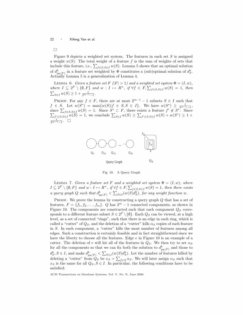
Lemma 7. Given a feature set F and a weighted set system Φ = (I, w), whereI ⊆ 2F \ ∅, F and w : I 7→ R+, if ∀f ∈ F,
∑
f∈S,S∈I w(S) = 1, then there exists
a query graph Q such that dkgΦ(F ) <
∑
S∈I(w(S)dkS), for any weight function w.
Proof. We prove the lemma by constructing a query graph Q that has a set offeatures, F = f1, f2, . . . , fm. Q has 2m − 1 connected components, as shown inFigure 10. The components are constructed such that each component QS corre-sponds to a different feature subset S ∈ 2F \∅. Each QS can be viewed, at a highlevel, as a set of connected “rings”, such that there is an edge in each ring, which iscalled a “cutter” of QS , and the deletion of a “cutter” kills αS copies of each featurein S. In each component, a “cutter” kills the most number of features among alledges. Such a construction is certainly feasible and in fact straightforward since wehave the liberty to choose all the features. Edge e in Figure 10 is an example of acutter. The deletion of e will hit all of the features in QS . We then try to set αS
for all the components so that we can fix both the solution to dkgΦ(F ) and those to
dkS , S ∈ I, and make dk
gΦ(F ) <∑
S∈I(w(S)dkS). Let the number of features killed by
deleting a “cutter” from QS be xS =∑
f∈S αS . We will later assign αS such thatxS is the same for all QS , S ∈ I. In particular, the following conditions have to besatisfied:
ACM Transactions on Database Systems, Vol. V, No. N, June 2006.
Feature-based Similarity Search in Graph Structures · 23
(1) The solution to dkgΦ(F ) is the full feature set F . This means the k edges to be
deleted must all be the “cutter” in component QF . In this case, since each“cutter” kills
∑
f∈F
αF
∑
f∈S,S∈I
w(S)
=∑
f∈F
αF = mαF
features, to make deleting a “cutter” in QF more profitable than in any otherQS , S ∈ I, it has to be that
mαF > xS
(2) For S ∈ I, dkS = kxS . This means none of the k “cutter”s to be deleted lies in
component QF . For this to happen, deleting a “cutter” in QS has to be moreprofitable than in QF for all feature subset S ∈ I. A “cutter” in QS kills xS
features and a “cutter” in QF kills at most |S|αF . Since S ⊂ F , |S| ≤ m − 1.Thus, it has to be that
(m − 1)αF < xS
(3) For any w satisfying ∀f ∈ F,∑
f∈S,S∈I w(S) = 1,
kmαF <∑
S∈I
w(S)xS
Due to Lemma 6, we have∑
S∈I w(S) ≥ 1+ 12m−1−1 . Set xS = αF m(1+ 1
21
2m−1−1 ) =
αF m 2m−12m . It is easy to verify that all three conditions are satisfied with this xS .
Lemma 8. There exist a query graph Q and a feature set F , such that none ofthe inequalities in the corresponding inequality system Ax ≥ b is redundant.
Proof. Because every feature is chosen in 2m−1 different feature sets, any givencolumn of A thus consists exactly 2m−1 1s and 2m−1 − 1 0s. Recall that dk
F isdefined to be the maximum number of features in a chosen feature set F that canbe killed by deleting k edges from a query graph. Therefore, b ≥ 0.
Take from the system the i-th inequality Aix ≥ bi. Let A′x ≥ b′ be the resultingsystem after deleting this inequality. We prove that this inequality is not redundantrelative to A′x ≥ b′.
It is obvious that A′x ≥ b′ is solvable, since by assigning values large enoughto all the variables, all inequalities can be satisfied. The feasible region is indeedunbounded. We are left to show that there exists no such row vector u ∈ R2m−2
satisfying
u ≥ 0,Ai ≥ uA′,ub′ ≥ bi.
As there are exactly 2m−1 1s in every column c 6∈ π(Ai) of A′, in order to satisfyu ≥ 0,Ai ≥ uA′, it has to be that uj = 0, j ∈ π(A′
c). We prove that for all suchu, ub′ < bi.
Let H = π(Ai) and θπ((A′)i) = ui. For any S ⊆ 1, 2, . . . ,m, denote the
feature set FS = fi|i ∈ S. Define a weighted set system Φ = (I, w), I = 2H \
ACM Transactions on Database Systems, Vol. V, No. N, June 2006.

24 · Xifeng Yan et al.
∅,H, w(S) = θS , S ∈ I, and function gΦ : F 7→ R+, gΦ(fi) =∑
i∈S,S∈I w(S).Let D(F ) ⊆ F be the set of deleted features corresponding to any solution ofdk
F . Observe that since Ai ≥ uA′, for 1 ≤ j ≤ m,∑
j∈S θS ≤ 1. Also note that
bi =∑
j∈π(Ai) vj − dkF
π(Ai)=
∑
j∈H vj − dkFH
.
ub′ − bi =∑
S∈I
θS
∑
j∈S
vj − dkFS
−
∑
j∈H
vj − dkFH
=∑
S∈I
θS
∑
j∈S
vj − dkFS
−∑
j∈H
vj
∑
j∈S,S∈I
θS + (1 −∑
j∈S,S∈I
θS)
+dkFH
=∑
S∈I
θS
∑
j∈S
vj −∑
j∈H
vj
∑
j∈S,S∈I
θS −∑
j∈H
vj(1 −∑
j∈S,S∈I
θS)
+dkFH
−∑
S∈I
θSdkFS
=∑
j∈1,2,...,m
vj
∑
j∈S,S∈I
θS −∑
j∈H
vj
∑
j∈S,S∈I
θS −∑
j∈H
vj(1 −∑
j∈S,S∈I
θS)
+dkFH
−∑
S∈I
θSdkFS
= −∑
j∈H
vj(1 −∑
j∈S,S∈I
θS) + dkFH
−∑
S∈I
θSdkFS
We distinguish two possible cases here:
(1) If ∃j,∑
j∈S,S∈I θS < 1, let kj be the number of features killed for feature fj in
the solution to dkFH
, we write the above expression as
ub′ − bi = −∑
j∈H
vj(1 −∑
j∈S,S∈I
θS) +∑
fj∈D(FH)
kj(1 −∑
j∈S,S∈I
θS)
∑
fj∈D(FH)
kj
∑
j∈S,S∈I
θS −∑
S∈I
θSdkFS
≤ −∑
j∈H
vj(1 −∑
j∈S,S∈I
θS) +∑
fj∈D(FH)
kj(1 −∑
j∈S,S∈I
θS)
+dkgΦ(FH) −
∑
S∈I
θSdkFS
By definition, D(FH) ⊆ FH , and there exist a query graph Q and a feature setF such that kj < vj , for fj ∈ D(FH). Since dk
gΦ(FH) ≤∑
S∈I θSdkFS
, in this
case ub′ − bi < 0.
ACM Transactions on Database Systems, Vol. V, No. N, June 2006.

Feature-based Similarity Search in Graph Structures · 25
(2) If ∀j,∑
j∈S,S∈I θS = 1,
ub′ − bi = dkFH
−∑
S∈I
θSdkFS
= dkgΦ(FH) −
∑
S∈I
θSdkFS
Since we have proved in Lemma 7 that there exists a query graph Q anda feature set F , such that, for any u ≥ 0 satisfying ∀j,
∑
j∈S,S∈I θS = 1,
dkgΦ(FH) <
∑
S∈I θSdkFS
. It follows that in this case ub′ − bi < 0.
Therefore we have ub′ − bi < 0. As such, there exists no such a row vectoru ∈ R2m−2 satisfying
u ≥ 0,Ai ≥ uA′,ub′ ≥ bi.
Now that we have established these lemmas in the modified definition of r(ui, vi)in Definition (11), it is time to go back to our original Definition (7). For anyselected feature set Fi, let F ′
i = fj |fj ∈ Fi, uj ≥ vj. Then the inequality ofFi becomes
∑
xi∈Fi\F ′
ixi ≥
∑
xi∈Fi\F ′
ivi − dk
Fi. Since we have dk
Fi\F ′
i≤ dk
Fi, the
hyperplane defined by this inequality always lies outside the feasible region of thehalfspace defined by
∑
xi∈Fi\F ′
ixi ≥
∑
xi∈Fi\F ′
ivi − dk
Fi\F ′
i, and the latter is an
inequality of the inequality system in our proved lemma. Since a hyperplane hasto intersect the current feasible region to invalidate the nonredundancy of anyinequality, this means adding these hyperplanes will not make any of the inequalitiesin the system redundant. By definition of redundant constraint, Lemma (8) alsoholds under the original definition of r(ui, vi) in Definition (7).
We now prove the lower bound on the complexity of the feature set selectionproblem by adversary arguments, a technique that has been widely used in compu-tational geometry to prove lower bounds for many fundamental geometric problems[Kislicyn 1964, Erickson 1996]. In general, the arguments works as follows. Any al-gorithm that correctly computes output must access the input. Instead of queryingan input chosen in advance, imagine an all-powerful malicious adversary pretends tochoose an input, and answers queries in whatever way that will make the algorithmdo the most work. If the algorithm does not make enough queries, there will beseveral different inputs, each consistent with the adversary’s answers, that shouldresult in different outputs. Whatever the output of the algorithm, the adversarycan reveal an input that is consistent with all of its answers, yet inconsistent withthe algorithms’s output. Therefore any correct algorithm would have to make themost queries in the worst case.
Theorem 3. [Single Feature Set Selection Problem] Suppose F = f1, f2, . . . , fmis the set of all features in query graph Q. In the worst case, it takes Ω(2m) stepsto compute Fopt such that |ΓFopt
| = maxF ′⊆F |ΓF ′ |.
Proof. Given a query graph Q, imagine an adversary has the N points at hisdisposal, each corresponding to an indexed graph. For any algorithm A to computeFopt, it would have to determine if there exists a halfspace defined by a feature set
ACM Transactions on Database Systems, Vol. V, No. N, June 2006.

26 · Xifeng Yan et al.
F ′ that could prune more points than the current best choice. Assume that A hasto compare a point with the hyperplane in order to know if the point lies in thehalfspace. Suppose that it stops after checking k inequalities and claims that Fopt
is found. Let S be the current feasible region formed by these k halfspaces. Thefollowing observations are immediate.
(1) Placing any new point inside S does not change the number of points that canbe pruned by any F ′ already checked, i.e., the current best choice remains thesame.
(2) Any unchecked inequality corresponds to a hyperplane that will “cut” off anonempty convex subspace from S since it is not redundant.
Then a simple strategy for the adversary is to always keep more than half of the Npoints in hand. Whenever A stops before checking all the 2m − 1 inequalities andclaims an answer for Fopt, the adversary can put all the points in hand into thenonempty subspace of the current feasible region that would be cut off by adding anunchecked inequality. Since now this inequality prunes more points than any otherinequality as yet, the algorithm A thus would fail in computing Fopt. Therefore, inthe worst case, any algorithm would have to take Ω(2m) steps to compute Fopt
Corollary 1. [Fixed Number of Feature Sets Selection Problem] Suppose F =f1, f2, . . . , fm is the set of all features in query graph Q. In the worst case, ittakes Ω(2m) steps to compute SF = F ′|F ′ ⊆ F, |SF | = c such that SF prunes themost number of graphs for any set of c feature sets, where c is a constant.
Proof. The proof is by an argument similar to that in Theorem 3. Since anadversary can always keep more than half of the N points in hand, and choose,depending on the output of the algorithm, whether or not to place them in thenonempty polytope cut off by an inequality that has not been checked; and the al-gorithm, before checking the corresponding inequality, has no access to this knowl-edge; any correct algorithm would fail if it announces an optimal set of c featuresets before Ω(2m) steps.
Corollary 2. [Multiple Feature Sets Selection Problem] Suppose F = f1, f2,. . . , fm is the set of all features in query graph Q. In the worst case, it takes Ω(2m)steps to compute the smallest candidate set.
Proof. The proof is by an argument similar to that in Theorem 3 and Corollary1.
Theorem 3 shows that to prune the most number of graphs in one access to theindex structure, it takes exponential time in the number of features in the worstcase. Corollary 1 shows that even if we want to compute a set of feature sets suchthat, used one after another, they prune the most graphs with multiple accesses tothe index, such an optimal set is also hard to compute.
5.3 Clustering based Feature Set Selection
Theorem 3 shows that it takes an exponential number of steps to find an optimalsolution in the worst case. In practice, we are interested in the heuristics thatare good for a large number of query graphs. We use selectivity defined below tomeasure the filtering power of a feature f for all graphs in the database.
ACM Transactions on Database Systems, Vol. V, No. N, June 2006.

Feature-based Similarity Search in Graph Structures · 27
Definition 5 Selectivity. Given a graph database D, a query graph Q, and afeature f , the selectivity of f is defined by its average frequency difference within Dand Q, written as δf (D,Q). δf (D,Q) is equal to the average of r(u, v), where u isa variable denoting the frequency of f in a graph belonging to D, v is the frequencyof f in Q, and r is defined in Equation (7).
Using the feature-graph matrix, we need not access the physical database tocalculate selectivity. Since selectivity is dependent on the graphs in the databaseas well as the query graph, it needs to be computed for every query and is not partof preprocessing. However, we can sample the feature-graph matrix to acceleratethe computation of the selectivity for a given feature.
To put features with the same filtering power in a single filter, we have to groupfeatures with similar selectivity into the same feature set. Before we elaborate thisidea, we first conceptualize three general principles that provide guidance on featureset selection.
Principle 1. Select a large number of features.
Principle 2. Make sure features cover the query graph uniformly.
Principle 3. Separate features with different selectivity.
Obviously, the first principle is necessary. If only a small number of features areselected, the maximum allowed feature misses may become very close to
∑n
i=1 vi.In that case, the filtering algorithm loses its pruning power. The second principleis more subtle than the first one, but both based on the same intuition. If most ofthe features cover several common edges, the relaxation of these edges will makethe maximum allowed feature misses too big. The third principle has been exam-ined above. Unfortunately, these three criteria are not consistent with each other.For example, if we use all the features in a query, the second and the third princi-ples will be violated since sparse graphs such as chemical structures have featuresconcentrated in the graph center. Secondly, low selective features deteriorate thepotential filtering power from high selective ones due to frequency conjugation. Onthe other hand, we cannot use the most selective features alone because we maynot have enough highly selective features in a query.
Since using a single filter with all the features included is not expected to performwell, we devise a multi-filter composition strategy: Multiple filters are constructedand coupled together, where each filter uses a distinct and complementary featureset. The three principles we have examined provide general guidance on how tocompose the feature set for each of the filters. The task of feature set selectionis to make a trade-off among these principles. We may group features by theirsize to create feature sets. This simple scheme satisfies the first and the secondprinciples. Usually the selectivity of features with varying sizes is different. Thusit also roughly meets the third principle. This simple scheme actually works asverified by our experiments. However, we may go one step further by first groupingfeatures with similar size and then clustering them based on their selectivity toform feature sets.
We devise a simple hierarchical agglomerative clustering algorithm based on theselectivity of the features. The final clusters produced represent the distinct featuresets for the different filters. The algorithm starts at the bottom, where each feature
ACM Transactions on Database Systems, Vol. V, No. N, June 2006.

28 · Xifeng Yan et al.
is an individual cluster. At each level, it recursively merges the two closest clustersinto a single cluster. The “closest” means their selectivity is the closest. Eachcluster is associated with two parameters: the average selectivity of the cluster andthe number of features associated with it. The selectivity of two merged clusters isdefined by a linear interpolation of their own selectivity,
n1δ1 + n2δ2
n1 + n2, (12)
where n1 and n2 are the number of features in the two clusters, and δ1 and δ2 aretheir corresponding selectivity.
f 1 f 2 f 3 f 4 f 5 f 6
3 clusters
Fig. 11. Hierarchical Agglomerative Clustering
Features are first sorted according to their selectivity and then clustered hierar-chically. Assume that δf1
(D,Q) ≤ δf2(D,Q) ≤ . . . ≤ δf6
(D,Q) . Figure 11 showsa hierarchical clustering tree. In the first round, f5 is merged with f6. In the secondround, f1 is merged with f2. After that, f4 is merged with the cluster formed byf5 and f6 if f4 is the closest one to them. Since the clustering is performed in onedimension, it is very efficient to build.
6. ALGORITHM IMPLEMENTATION
In this section, we formulate our filtering algorithm, called Grafil (Graph SimilarityFiltering).
Grafil consists of two components: a base component and a clustering component.Both of them apply the multi-filter composition strategy. The base componentgenerates feature sets by grouping features of the same size and uses them to filtergraphs based on the upper bound of allowed feature misses derived in Section 4.4. Itfirst applies the filter using features with one edge, then the one using features withtwo edges, and so on. We denote the base component by Grafil-base. The clusteringcomponent combines the features whose sizes differ by at most 1, and groups themby their selectivity values. Algorithm 3 sketches the outline of Grafil. Fi in Line 2represents the set of features with i edges. Lines 2-4 form the base component andLines 5-11 form the clustering component. Once the hierarchical clustering is doneon features with i edges and i + 1 edges, Grafil divides them into three groups withhigh selectivity, medium selectivity, and low selectivity, respectively. A separatefilter is constructed based on each group of features. For the hierarchical clusters
ACM Transactions on Database Systems, Vol. V, No. N, June 2006.

Feature-based Similarity Search in Graph Structures · 29
Algorithm 3 Grafil
Input: Graph database D, Feature set F ,Maximum feature size maxL, andA relaxed query Q.
Output: Candidate answer set CQ.
1: let CQ = D;2: for each feature set Fi, i ≤ maxL do
3: calculate the maximum feature misses dmax;4: CQ = G|d(G,Q) ≤ dmax, G ∈ CQ ;5: for each feature set Fi
⋃
Fi+1, i < maxL do
6: compute the selectivity based on CQ;7: do the hierarchical clustering on features in Fi
⋃
Fi+1;8: cluster features into three groups, X1, X2, and X3;9: for each cluster Xi do
10: calculate the maximum feature misses dmax;11: CQ = G|d(G,Q) ≤ dmax, G ∈ CQ ;12: return CQ;
shown in Figure 11, Grafil will choose f1 and f2 as group 1, f3 as group 2, and f4,f5 and f6 as group 3.
To deploy the multiple filters, Grafil can run in a pipeline mode or a parallelmode. The diagram in Figure 12 depicts the pipeline mode, where the candidateanswer set returned from the current step is pumped into the next step.
Query feature set 1
feature set n
...
C 1
C n
Fig. 12. Filtering Pipeline
Algorithm 3 is written in the pipeline mode. We can change it to the parallelmode by replacing Line 4 and Line 11 with the following statement,
CQ = G|d(G,Q) ≤ dmax, G ∈ D ,
and CQ in Line 6 with D. With these modifications, Grafil can be parallelizeddirectly. The final candidate answer set is the intersection of the candidate setsreturned by each filter. However, there is a slight difference between the pipelinemode and the parallel mode. Grafil in the pipeline mode can achieve a smallercandidate answer set. The reason is the clustering component (Line 6) in thepipeline mode calculates the selectivity based on the candidate graphs returned in
ACM Transactions on Database Systems, Vol. V, No. N, June 2006.

30 · Xifeng Yan et al.
the previous step, while the parallel mode does not. We will show the performanceimpact raised by this difference in the next section.
7. EMPIRICAL STUDY
In this section, we conduct several experiments to examine the properties of Grafil.The performance of Grafil is compared with two algorithms based on a single filter:one using individual edges as features (denoted as Edge) and the other using allfeatures of a query graph (denoted as Allfeature). Many similarity search algorithms[Hagadone 1992, Raymond et al. 2002] can only apply the edge-based filteringmechanism since the mapping between edge deletion/relabeling and feature misseswas not established before this study. In fact, the edge-based filtering approach canbe viewed as a degenerate case of the feature-based approach using a filter withsingle edge features. By demonstrating the conditions where Grafil can filter moregraphs than Edge and Allfeature, we show that Grafil can substantially improvesubstructure similarity search in large graph databases.
Two kinds of datasets are used throughout our empirical study: one real datasetand a series of synthetic datasets. The real dataset is an AIDS antiviral screendataset containing the topological structures of chemical compounds. This datasetis available on the website of the Developmental Therapeutics Program (NCI/NIH)3.In this dataset, thousands of compounds have been checked for evidence of anti-HIVactivity. The dataset has around 44,000 structures. The synthetic data generatorwas kindly provided by Kuramochi et al. [Kuramochi and Karypis 2001]. The gen-erator allows the user to specify various parameters, such as the database size, theaverage graph size, and the label types, to examine the scalability of Grafil.
We built Grafil based on the gIndex algorithm [Yan et al. 2004]. gIndex firstmines frequent subgraphs with size up to 10 and then retains discriminative onesas indexing features. We thus take the discriminative frequent structures as ourindexing features. Certainly, other kinds of features can be used in Grafil too, sinceGrafil does not rely on the kinds of features to be used. For example, Grafil can alsotake paths [Shasha et al. 2002] as features to perform the similarity search.
Through our experiments, we illustrate that
(1) Grafil can efficiently prune the search space for substructure similarity searchand generate up to 15 times fewer candidate graphs than the alternatives inthe chemical dataset.
(2) Bound refinement and feature set selection for the multiple filter approachdeveloped by Grafil are both effective.
(3) Grafil performs much better for graphs with a small number of labels.
(4) The single filter approach using all features together does not perform well dueto the frequency conjugation problem identified in Section 5. Neither does theapproach using individual edges as features due to their low selectivity.
Experiments on the Chemical Compound Dataset.
We first examine the performance of Grafil over the AIDS antiviral database. Thetest dataset consists of 10, 000 graphs that are randomly selected from the AIDS
3http://dtpsearch.ncifcrf.gov/FTP/AIDO99SD.BIN
ACM Transactions on Database Systems, Vol. V, No. N, June 2006.

Feature-based Similarity Search in Graph Structures · 31
screen database. These graphs have 25 nodes and 27 edges on average. The largestone has 214 nodes and 217 edges in total. Note that in this dataset most of the atomsare carbons and most of the edges are carbon-carbon bonds. This characteristicmakes the substructure similarity search very challenging. The query graphs aredirectly sampled from the database and are grouped together according to theirsize. We denote the query set by Qm, where m is the size of the graphs in Qm. Forexample, if the graphs in a query set have 20 edges each, the query set is writtenas Q20. Different from the experiment setting in [Yan et al. 2004], the edges in ourdataset are assigned with edge types, such as single bond, double bond, and so on.By doing so, we reduce the number of exact substructure matches for each querygraph. This is exactly the case where the substructure similarity search will help:find a relatively large matching set by relaxing the query graph a little bit. Whena user submits a substructure similarity query, he may not allow arbitrary deletionof some critical atoms and bonds. In order to simulate this constraint, we retain25% of the edges in each query graph.
104
103
102
10 0 1 2 3 4 5
# of
can
dida
te a
nsw
ers
# of edge relaxations
EdgeAll
Grafil
Fig. 13. Structure Query with 16 edges
We made some slight modifications to the Allfeature approach by removing fea-tures whose size is greater than the query graph size divided by the number of edgerelaxations. This modification improves the performance of Allfeature. Figure 13depicts the performance of Edge, Allfeature and Grafil for the query set Q16. TheX-axis shows the number of edge relaxations done for a query graph. The Y -axisshows the average number of candidate graphs returned by each algorithm. Asexplained in Section 1, it is always preferable to filter as many graphs as possiblebefore performing real similarity computation. The accurate pairwise similaritychecking is very time-consuming. If we allow one edge to be lost for queries with16 edges, the Edge approach can prune 96% of the dataset while Grafil can prune99.7%. If a user wants to check whether there are real matches in the remaining0.3% of the dataset, they can apply the similarity computation tools developed in[Hagadone 1992, Raymond et al. 2002] to check them. If they are not satisfied withthe result, the user can relax the edge loss to 3. The Edge approach will return18% of the dataset and Grafil will return 11% of the dataset. The running time ofGrafil is negligible in comparison to the accurate substructure similarity computa-tion. Using the feature-graph matrix, the filtering stage takes less than 1 secondper query for this query set.
ACM Transactions on Database Systems, Vol. V, No. N, June 2006.

32 · Xifeng Yan et al.
Figure 13 demonstrates that Grafil outperforms Edge and Allfeature significantlywhen the relaxation ratio is within 2 edges by a factor of 5-10 times. However,when the relaxation ratio increases, the performance of Grafil is close to Edge. Thereason is very simple. The structures of chemical compounds are very sparse, andare mainly tree-structured with several loops embedded. If we allow three edges tobe deleted or relabeled for a query that has 16 edges, it is likely that the relaxededges divide the query graph into four pieces. Each piece may only have 4-5 edges intotal which virtually cannot hold any significant features. These small pieces havevery weak pruning power. Eventually, only the number of remaining edges in aquery graph counts. Therefore, we expect that when the relaxation ratio increases,Grafil will have performance close to Edge. However, at this time the number ofmatches will increase dramatically. Since a user may not like the relaxed querygraph to deviate too far away from her/his need, she/he may stop with a smallrelaxation ratio. Take the query set Q16 as an example, on average it only has 1.2exact substructure matches. If we allow two edges to be relaxed, it has 12.8 matcheson average, which may be enough for examination. And this figure is proportionalto the number of graphs in the database.
The above result is further confirmed through another experiment. We test thequeries that have 20 edges. Figure 14 shows the performance comparison amongthese three algorithms. Again, Grafil outperforms Edge and Allfeature.
104
103
102
10
1 0 1 2 3 4 5
# of
can
dida
te a
nsw
ers
# of edge relaxations
EdgeAll
Grafil
Fig. 14. Structure Query with 20 edges
0 200 400 600 800
1000 1200 1400 1600 1800 2000
0 1 2 3 4 5
# of
can
dida
te a
nsw
ers
# of edge relaxations
with bound refinementwithout bound refinement
Fig. 15. Feature Miss Estimation Refinement
ACM Transactions on Database Systems, Vol. V, No. N, June 2006.
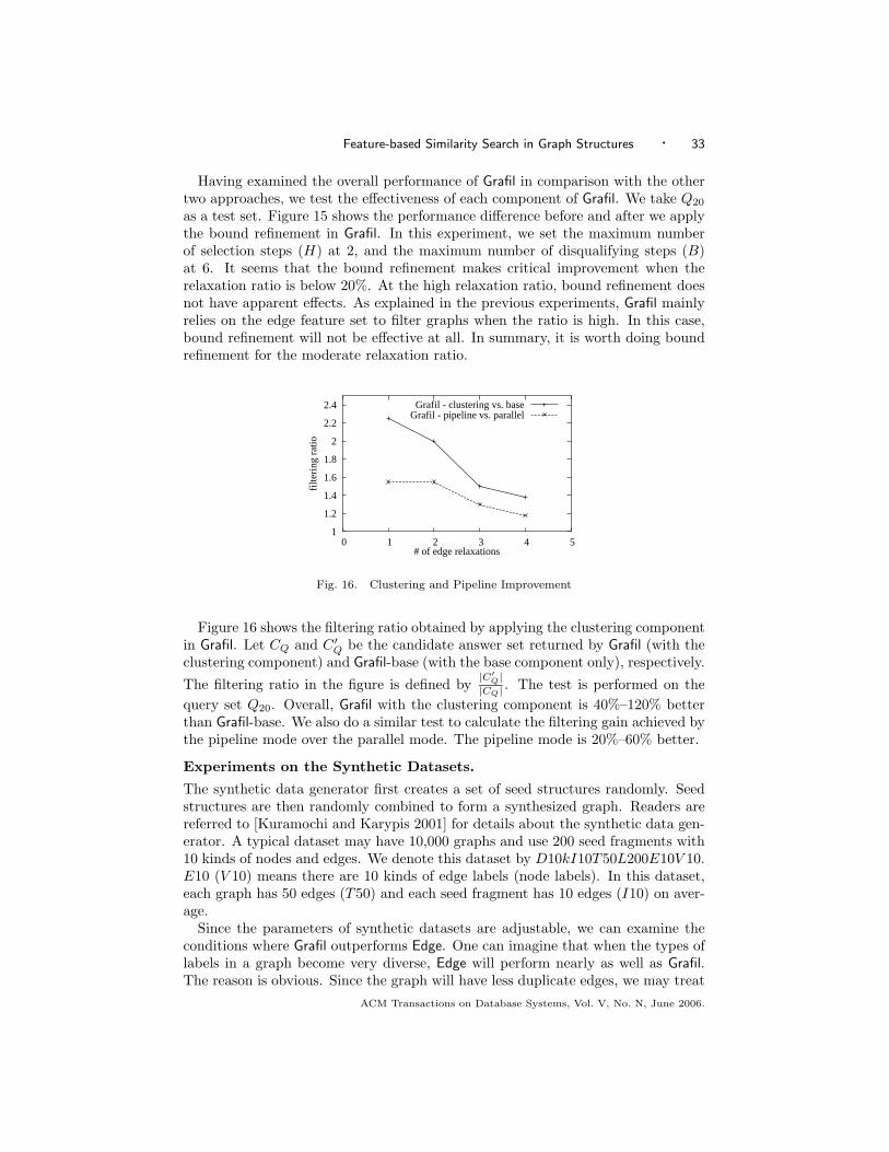
Feature-based Similarity Search in Graph Structures · 33
Having examined the overall performance of Grafil in comparison with the othertwo approaches, we test the effectiveness of each component of Grafil. We take Q20
as a test set. Figure 15 shows the performance difference before and after we applythe bound refinement in Grafil. In this experiment, we set the maximum numberof selection steps (H) at 2, and the maximum number of disqualifying steps (B)at 6. It seems that the bound refinement makes critical improvement when therelaxation ratio is below 20%. At the high relaxation ratio, bound refinement doesnot have apparent effects. As explained in the previous experiments, Grafil mainlyrelies on the edge feature set to filter graphs when the ratio is high. In this case,bound refinement will not be effective at all. In summary, it is worth doing boundrefinement for the moderate relaxation ratio.
1
1.2
1.4
1.6
1.8
2
2.2
2.4
0 1 2 3 4 5
filte
ring
rat
io
# of edge relaxations
Grafil - clustering vs. baseGrafil - pipeline vs. parallel
Fig. 16. Clustering and Pipeline Improvement
Figure 16 shows the filtering ratio obtained by applying the clustering componentin Grafil. Let CQ and C ′
Q be the candidate answer set returned by Grafil (with theclustering component) and Grafil-base (with the base component only), respectively.
The filtering ratio in the figure is defined by|C′
Q|
|CQ| . The test is performed on the
query set Q20. Overall, Grafil with the clustering component is 40%–120% betterthan Grafil-base. We also do a similar test to calculate the filtering gain achieved bythe pipeline mode over the parallel mode. The pipeline mode is 20%–60% better.
Experiments on the Synthetic Datasets.
The synthetic data generator first creates a set of seed structures randomly. Seedstructures are then randomly combined to form a synthesized graph. Readers arereferred to [Kuramochi and Karypis 2001] for details about the synthetic data gen-erator. A typical dataset may have 10,000 graphs and use 200 seed fragments with10 kinds of nodes and edges. We denote this dataset by D10kI10T50L200E10V 10.E10 (V 10) means there are 10 kinds of edge labels (node labels). In this dataset,each graph has 50 edges (T50) and each seed fragment has 10 edges (I10) on aver-age.
Since the parameters of synthetic datasets are adjustable, we can examine theconditions where Grafil outperforms Edge. One can imagine that when the types oflabels in a graph become very diverse, Edge will perform nearly as well as Grafil.The reason is obvious. Since the graph will have less duplicate edges, we may treat
ACM Transactions on Database Systems, Vol. V, No. N, June 2006.

34 · Xifeng Yan et al.
it as a set of tuples node1 label, node2 label, edge label instead of a complexstructure. This result is confirmed by the following experiment. We generate asynthetic dataset, D10kI10T50L200 E10V 10, which has 10 edge labels and 10node labels. This setting will generate (10× 11)/2× 10 = 550 different edge tuples.Most of the graphs in this synthetic dataset have 30 to 100 edges. If we representa graph as a set of edge tuples, few edge tuples will be the same for each graph inthis dataset. In this situation, Edge is good enough for similarity search. Figure 17shows the results for queries with 24 edges. The two curves are very close to eachother, as expected.
5
10
15
20
25
0 1 2 3 4 5 6 7
# of
can
dida
te a
nsw
ers
# of edge relaxations
EdgeGrafil
Fig. 17. Numerous Types of Labels
We then reduce the number of label types in the above synthetic dataset and onlyallow 2 edge labels and 4 vertex labels. This setting significantly increases the selfsimilarity in a graph. Figure 18 shows that Grafil outperforms Edge significantly inthis dataset. We can further reduce the number of label types. For example, if weignore the label information and only consider the topological skeleton of graphs,the edge-based filtering algorithm will not be effective at all. In that situation,Grafil has more advantages than Edge.
10
102
103
104
0 1 2 3 4 5
# of
can
dida
te a
nsw
ers
# of edge relaxations
EdgeGrafil
Fig. 18. Few Types of Labels
ACM Transactions on Database Systems, Vol. V, No. N, June 2006.

Feature-based Similarity Search in Graph Structures · 35
8. CONCLUSIONS
In this study, we have investigated the problem of substructure similarity search inlarge scale graph databases, a problem raised by the emergence of massive, com-plex structural data. Different from the previous work, our solution explored thefiltering algorithm using indexed structural patterns, without doing costly struc-ture comparisons. The transformation of the structure-based similarity measure tothe feature-based measure renders our method attractive in terms of accuracy andefficiency. Since our filtering algorithm is fully built on the feature-graph matrix,it performs very fast without accessing the physical database. We showed thatthe multi-filter composition strategy adopted by Grafil is superior to the single fil-ter approach using all features together due to the frequency conjugation problemidentified in this article. Based on a geometric interpretation, the complexity ofoptimal feature set was analyzed in our study, which is Ω(2m) in the worst case. Inpractice, we identified several criteria to build effective feature sets for filtering anddemonstrated that the clustering-based feature selection can improve the filteringperformance further. The proposed feature-based indexing concept is very generalsuch that it can be applied to searching approximate non-consecutive sequences,trees, and other structured data as well.
REFERENCES
Beretti, S., Bimbo, A., and Vicario, E. 2001. Efficient matching and indexing of graph modelsin content based retrieval. IEEE Trans. on Pattern Analysis and Machine Intelligence 23,
1089–1105.
Berman, H., Westbrook, J., Feng, Z., Gilliland, G., Bhat, T., Weissig, H., Shindyalov, I.,
and Bourne, P. 2000. The protein data bank. Nucleic Acids Research 28, 235–242.
Bunke, H. and Shearer, K. 1998. A graph distance metric based on the maximal commonsubgraph. Pattern Recognition Letters 19, 255 – 259.
Erickson, J. 1996. Lower bounds for fundamental geometric problems. Ph.D. Thesis,Universityof California at Berkeley.
Feige, U. 1998. A threshold of ln n for approximating set cover. Journal of the ACM 45, 634 –
652.
Garey, M. and Johnson, D. 1979. Computers and Intractability: A Guide to the Theory ofNP-Completeness. Freeman & Co., New York.
Giugno, R. and Shasha, D. 2002. Graphgrep: A fast and universal method for querying graphs.Proc. 2002 Int. Conf. on Pattern Recognition (ICPR’02), 112–115.
Gravano, L., Ipeirotis, P., Jagadish, H., Koudas, N., Muthukrishnan, S., Pietarinen, L.,
and Srivastava, D. 2001. Using q-grams in a dbms for approximate string processing. DataEngineering Bulletin 24, 28–37.
Hagadone, T. 1992. Molecular substructure similarity searching: efficient retrieval in two-dimensional structure databases. J. Chem. Inf. Comput. Sci. 32, 515–521.
Hochbaum, D. 1997. Approximation Algorithms for NP-Hard Problems. PWS Publishing, MA.
Holder, L., Cook, D., and Djoko, S. 1994. Substructure discovery in the subdue system. In
Proc. AAAI’94 Workshop on Knowledge Discovery in Databases (KDD’94). 169 – 180.
Kailing, K., Kriegel, H., Schnauer, S., and Seidl, T. 2004. Efficient similarity search for
hierarchical data in large databases. In Proc. 9th Int. Conf. on Extending Database Technology(EDBT’04). 676–693.
Kanehisa, M. and Goto, S. 2000. Kegg: Kyoto encyclopedia of genes and genomes. Nucleic
Acids Research 28, 27–30.
Kislicyn, S. S. 1964. On the selection of the kth element of an ordered set by pairwise compar-
isons. Sibirskii Matematiceskii Zurnal (in Russian) 5, 557–564.
ACM Transactions on Database Systems, Vol. V, No. N, June 2006.

36 · Xifeng Yan et al.
Kuramochi, M. and Karypis, G. 2001. Frequent subgraph discovery. In Proc. 2001 Int. Conf.
on Data Mining (ICDM’01). 313–320.
Messmer, B. and Bunke, H. 1998. A new algorithm for error-tolerant subgraph isomorphism
detection. IEEE Trans. on Pattern Analysis and Machine Intelligence 20, 493 – 504.
Navarro, G. 2001. A guided tour to approximate string matching. ACM Computing Surveys 33,
31 – 88.
Nilsson, N. 1980. Principles of Artificial Intelligence. Morgan Kaufmann, Palo Alto, CA.
Padberg, M. 1995. Linear Optimization and Extensions. Springer-Verlag.
Petrakis, E. and Faloutsos, C. 1997. Similarity searching in medical image databases. Knowl-
edge and Data Engineering 9, 3, 435–447.
Raymond, J., Gardiner, E., and Willett, P. 2002. Rascal: Calculation of graph similarityusing maximum common edge subgraphs. The Computer Journal 45, 631–644.
Shasha, D., Wang, J., and Giugno, R. 2002. Algorithmics and applications of tree and graphsearching. In Proc. 21th ACM Symp. on Principles of Database Systems (PODS’02). 39–52.
Srinivasa, S. and Kumar, S. 2003. A platform based on the multi-dimensional data modelfor analysis of bio-molecular structures. In Proc. 2003 Int. Conf. on Very Large Data Bases
(VLDB’03). 975–986.
Ukkonen, E. 1992. Approximate string matching with q-grams and maximal matches. Theoretic
Computer Science, 191–211.
Ullmann, J. 1977. Binary n-gram technique for automatic correction of substitution, deletion,
insertion, and reversal errors in words. The Computer Journal 20, 141–147.
Wang, J., Zhang, K., Jeong, K., and Shasha, D. 1994. A system for approximate tree matching.IEEE Trans. on Knowledge and Data Engineering 6, 559 – 571.
Willett, P., Barnard, J., and Downs, G. 1998. Chemical similarity searching. J. Chem. Inf.Comput. Sci. 38, 983–996.
Yan, X., Yu, P., and Han, J. 2004. Graph indexing: A frequent structure-based approach. InProc. 2004 ACM Int. Conf. on Management of Data (SIGMOD’04). 335 – 346.
Yan, X., Yu, P., and Han, J. 2005. Substructure similarity search in graph databases. In Proc.2005 ACM Int. Conf. on Management of Data (SIGMOD’05). 766 – 777.
ACM Transactions on Database Systems, Vol. V, No. N, June 2006.


![An Efficient Probabilistic Approach for Graph …An Efficient Probabilistic Approach for Graph Similarity Search [Extended Technical Report] Zijian Li #1, Xun Jian #2, Xiang Lian](https://img.dokumen.tips/doc/110x75/5f1037bb7e708231d44805ae/an-eficient-probabilistic-approach-for-graph-an-eficient-probabilistic-approach.jpg)