Embed Size (px)
Citation preview

Feasibility Study: Oregon
Retirement Savings Plan
August 2016

Contents
Executive Summary ............................................................................................................................ 1 Detailed Feasibility Study ................................................................................................................... 4
Introduction ....................................................................................................................................... 4
Program Costs ................................................................................................................................... 5 Start-up Costs ................................................................................................................................ 6 Ongoing Costs ............................................................................................................................... 6
Program Revenue ............................................................................................................................ 10 Contributions to the Program ...................................................................................................... 10
Account Withdrawals and Growth ............................................................................................. 11 ORSP Finances ................................................................................................................................ 13
The “Break-even” Point .............................................................................................................. 13 Paying Off Initial Losses ............................................................................................................. 15
Alternative Scenarios ...................................................................................................................... 17 Conclusion ....................................................................................................................................... 20
Appendix A ......................................................................................................................................... 21 Appendix B ......................................................................................................................................... 23
Number of Active Participants .................................................................................................... 23
Number of Inactive Participants ................................................................................................. 27 Account Closures ........................................................................................................................ 30
Inactive Accounts Returning to Active ....................................................................................... 31

1
Executive Summary
The Oregon Retirement Savings Plan (ORSP) will require employers who offer no
retirement plan to automatically enroll their employees in a Roth IRA. For ORSP to succeed, it has
to be financially self-sufficient. The following analysis shows that ORSP will be cash-flow positive
(annual revenue will be equal to annual operating costs) within four years and net positive (revenue
will cover both start-up and operating costs) in seven years. These results are based on a set of
initial assumptions for program design and participant behavior, and include annual fees of 1.2
percent (or 120 basis points) on asset balances. Once start-up costs are paid back, fees can be
greatly reduced to as low as 30-50 basis points. These results hold under a variety of scenarios, but
the number of years needed to break even would go up if the state chooses a default contribution
rate that is below 5 percent, account maintenance costs are higher than expected, or initial fees are
set too low. Appendix A contains a range of outcomes based on alternative assumptions. Program
costs are based on discussions with Bridgepoint/Segal, other state feasibility studies, international
experience, costs faced by existing IRA providers, and discussions with the ORSP Board.
The initial assumptions regarding program design are threefold. First, the default
contribution rate is 5 percent, with auto-escalation to 10 percent. Second, contributions are invested
in a blended target date fund. Third, employers without a plan are enrolled in a staggered manner:
Year 1, employers with 50+ employees; Year 2, employers with 10+ employees and a payroll
provider; Year 3, all employers with 5 or more employees; and Year 5, employers with fewer than 5
employees.
This feasibility study first identifies the number of years that it takes the program, under the
initial assumptions, to become cash-flow positive and net positive, and the maximum size of the
deficit during the initial years. These results will inform the required length of a contract to attract
bids from recordkeepers or, alternatively, the size of a loan that ORSP might need to cover short-
term losses. The study then assesses how sensitive the program’s financial performance is to
changes in the underlying assumptions.
Under the program design laid out above, with revenues generated from asset management
fees of 120 basis points, the program becomes cash-flow positive in Year 4. As noted, in the long
run, costs as a share of assets will likely fall below 50 basis points, so the program can charge lower

2
fees in the longer term. These results are depicted in Figure 1, which shows program costs and
revenues, with revenues estimated under three alternative fee levels: 120, 100, and 50 basis points.
Clearly, higher fees cause the program to break even earlier, but – even under the lowest fee – the
program is cash flow positive in Year 10.
Figure 1. Estimated Ongoing Revenue and Costs of ORSP Under Initial Scenario, in Millions
Source: Center for Retirement Research at Boston College (CRR) calculations.
Figure 2 adds start-up costs to the analysis. It shows the program’s cumulative deficit from
both the ongoing costs and the fixed start-up costs, under the initial assumption of a 120-basis-point
fee. Under these assumptions, the program runs up a deficit of $23.9 million by Year 5 and then
begins running surpluses and paying the deficit down. The deficit is completely paid off by Year 7.
This finding suggests three strategies for managing the start-up years of the program. The first
alternative is to offer a recordkeeper a seven-year contract, which will allow it to use surpluses in
later years to eliminate any losses in the early years. The second option is for ORSP to take out a
loan to cover some of these upfront costs. ORSP could also combine these two approaches.
$0m
$20m
$40m
$60m
$80m
$100m
$120m
1 2 3 4 5 6 7 8 9 10 11 12 13 14 15
Program year
Ongoing costsRevenue (120 basis points)Revenue (100 basis points)Revenue (50 basis points)

3
Figure 2. Running ORSP Program Net Profits, in Millions, Assuming Fees of 120 Basis Points
Note: The loss increases slightly from Year 4 to Year 5, despite ongoing costs being covered, because of the enrollment
of employers with fewer than 5 employees at a per-employer cost of $200.
Source: CRR calculations.
Of course, these results could be sensitive to the underlying assumptions. The analysis
shows that the program is particularly vulnerable if either: 1) contribution rates are below 5 percent,
or 2) per-account costs are higher than expected. A fixed contribution rate of 3 percent increases the
number of the years for the program to become cash flow positive by three years and net positive by
five years. Increasing per-account costs by $10 – from $30 to $40 – has a slightly smaller effect,
with an increase of one year for cash flow positive and two years for net positive. However, the
program is not especially vulnerable to lower asset returns, higher-than-anticipated account
leakages, or higher rates of account closures as workers change jobs. In other words, early program
revenues are driven primarily by contributions and by early costs, primarily costs per account.
-$8.3m
-$14.8m
-$23.2m -$22.8m -$23.9m
-$12.8m
$4.6m
$28.6m
-$40m
-$20m
$0m
$20m
$40m
1 2 3 4 5 6 7 8
Plan year
4
Detailed Feasibility Study
Introduction
This study will evaluate the financial feasibility of the Oregon Retirement Savings Plan
(ORSP) using two metrics. The first metric is the time it takes for the program to become cash
positive or “self-sufficient,” i.e., for the fee revenue generated by account balances to exceed the
costs of creating and maintaining the accounts. The second metric is the time needed for the
program to become net positive, i.e., to generate enough revenue in excess of costs to pay back the
cost of starting up the program. This second metric will depend on the magnitude of the start-up
costs and how start-up costs are financed – one option is to give an outside vendor a long enough
contract to recoup any start-up costs and initial losses; a second option is for the ORSP to take out a
loan to finance these losses, with ORSP being paid back out of program revenue. In either case, it is
critical to that the program generates revenue in excess of operating costs within a short period of
time, with reasonable fees, and without accumulating large losses. This study will evaluate whether
the ORSP is likely to meet these goals.
Program and plan design can affect projections of costs and revenue; thus, the majority of
this study presents results under an initial program design and using a set of additional assumptions
on worker behavior. Under this initial design, employers who offer no retirement plan are required
to automatically enroll their employees in a Roth IRA at a default contribution rate of 5 percent with
auto-escalation over time to 10 percent. The initial scenario assumes that all employers without a
plan will be enrolled, but in a staggered manner: in Year 1, employers with 50+ employees will be
enrolled; in Year 2, employers with 10+ employees and a payroll provider; in Year 3, employers
with 5 or more employees; and in Year 5 employers with fewer than 5 employees. The study
initially assumes account holders’ money is invested in a blended target date fund.
The study makes several other assumptions, including population growth, worker
participation, worker mobility, and withdrawals. Perhaps the most important of these is that the
majority of workers participate in the program – our Market Research Report suggests 79 percent of
full-time and 76 percent of part-time workers will participate. The justifications for all of these
assumptions are discussed in detail in the Appendix B to this report. Because the final program
design has not been determined and because any one assumption may differ once the program is
implemented, the study will also present analyses to test the sensitivity of our results to changes in
participation, costs, account closures, and other assumptions that may affect program outcomes.

5
This study is organized as follows. The first section estimates the start-up and ongoing costs
of the ORSP. The second section estimates program revenue, which is ultimately collected as a
fraction of total account balances and which, in turn, depends on eligible worker participation, the
contribution rate, asset returns, and account withdrawals. The third section projects how costs and
revenue will interact to determine when the program becomes self-sufficient and when any initial
losses will be covered, as well as how these losses might be financed. The fourth section provides
insight into how alternative program designs and economic assumptions might affect estimates of
costs, revenue, and the time needed to break even. The final section concludes that, under the initial
assumptions for program design, revenue will equal operating costs within the first four years, and
that the start-up costs and operating losses over this time period would be less than $24 million, a
sum that could be paid back by Year 7 with program fees of 120 basis points.
Program Costs
ORSP’s costs fall into two broad categories: 1) the start-up costs associated with creating the
program and bringing on employers; and 2) the ongoing administrative costs associated with
maintaining accounts, serving participants, and managing investments. Figure 1 illustrates these
costs schematically, highlighting two drivers of start-up costs: 1) the number of employers that must
be brought into ORSP; and 2) the number of accounts that must be administered.
Figure 1. ORSP Costs
Start-up
costs
Ongoing
costs
One-time fixed cost to ORSP
Cost per employer
Recordkeeper’s cost
Investment cost as share of assets
Annual account administration cost
Total ORSP
costs
x # employers
x # accounts

6
Start-up Costs
Start-up costs reflect two realities: 1) presently, an auto-IRA program like the ORSP does
not exist; and 2) one of third-party recordkeepers’ biggest costs is connecting to individual
employers. The first fact means that an initial fixed cost of developing the program’s required
infrastructure will need to be paid by the ORSP or borne by a recordkeeper. Based on information
from other state auto-IRA studies, as well as consultations with the ORSP Board, the fixed cost of
developing the infrastructure to run the program was assumed to $993,000. The second fact means
that an additional charge must be anticipated by the recordkeeper to enroll each employer. After
consultation with Segal/Bridgepoint, the study assumes a cost of $200 per employer to reflect the
average cost of bringing on new employers.1 Because some of the more than 64,000 employers
described in the Market Research Report who may be affected by the ORSP may choose to offer a
private sector plan, the study assumes only 80 percent of eligible employers end up participating
(which is projected to translate to 20 percent of eligible employees). These assumptions yield a
start-up cost estimate of over $11 million – $1 million in fixed costs and $10 million to enroll the
51,000 employers affected by the program who do not switch over to a private sector plan.2 Figure
1A updates Figure 1 to include these start-up costs.
Figure 1A. Summary of Start-up Costs
Ongoing Costs
The next driver of overall cost is the per-account administration cost, which the
recordkeeper charges to keep track of account funds, provide statements, cover call centers, and
1 Onboarding an employer involves getting information from an employer to a recordkeeper to auto-enroll workers and
set-up accounts, and also setting up an interface between an employer’s payroll system and the recordkeeping platform to
process ongoing payroll deductions. 2 The start-up costs associated with connecting employers to ORSP is paid over the first five years of the program, as it is
rolled out to more employers.
Start-up
costs
One time fixed cost
$1 million
Cost per employer
$200 x
# employers
51,000
Total start-up
ORSP costs
11m

7
maintain the program’s website for account holders. The administration cost also covers transaction
costs associated with money coming into the program and money going out of the program through
distributions. After consultation with Segal/Bridgepoint on the operating model being considered,
this report assumes a per-account cost of $30 per year.
The contribution of account administrative costs to ORSP’s total costs largely depends on
the number of accounts. In this study, two types of accounts exist: active and inactive. In active
accounts, an individual is employed at an employer without a plan and is contributing to the plan.
Inactive accounts are maintained by someone who is not employed at an eligible employer but who
has not closed out their account. Given the initial scenario, the number of active accounts is
presented in Table 1.3
Table 1. Number of Active Full- and Part-time Participants in the ORSP
Year 3 Year 5 Year 10 Year 15
Full-time 265,000 297,000 304,000 312,000
Part-time 74,000 83,000 85,000 87,000
Total 349,000 380,000 389,000 399,000
Source: CRR calculations.
Inactive accounts are assumed to come from two types of employees who exit the program
and do not close their accounts: 1) workers who become unemployed; and 2) workers who switch to
an employer that offers a retirement plan. The rates at which individuals transition from active to
unemployed and from active to ineligible are based on the Survey of Income and Program
Participation (SIPP) and described in detail in Appendix B; the basic assumption is that each year,
85 percent of active accounts remain active, while 9 percent become inactive.4 The number of
inactive full- and part-time accounts is shown in Table 2.
3 For a more detailed description of how these estimates were obtained, see Appendix B.
4 The remaining 6 percent of accounts close, which is discussed in more detail in the revenue section of this report. Once
inactive, some workers do reenter the program. Each year, 5 percent of inactive workers in the covered sector are
assumed to return to eligibility, and workers who become unemployed are assumed to reenter the program the next year.
For more details, see Appendix B.

8
Table 2. Number of Inactive Full- and Part-time Participants in the ORSP
Year 3 Year 5 Year 10 Year 15
Full-time 24,000 47,000 83,000 100,000
Part-time 10,000 19,000 30,000 35,000
Total 34,000 66,000 113,000 135,000
Source: CRR calculations.
Combining Tables 1 and 2 and assuming the $30 per-account administrative cost allows the
calculation of total account administrative costs, as shown in Table 3. Because these administrative
costs are sensitive to several assumptions made so far, Box 1 highlights how costs would change
under alternative assumptions.
Table 3. Annual Account Administrative Costs
Year 3 Year 5 Year 10 Year 15
Active accounts 349,000 380,000 389,000 399,000
Inactive accounts 34,000 66,000 113,000 135,000
Total accounts 383,000 446,000 502,000 534,000
x cost per $30 $30 $30 $30
Account admin. costs $11.5m $13.4m $15.1m $16.0m Source: CRR calculations and discussions with Segal/Bridgepoint.
Box 1. Account Administrative Costs under Alternative Assumptions
Because administrative costs are driven by the number of accounts, costs are lower with fewer
accounts. For example, assume that participation is 50 percent, and 50 percent of workers exiting
the program close their accounts (the initial case is 75-80 percent participating and 20 percent
closing accounts). In this case, by program Year 15, there would be 308,000 accounts resulting in
account administrative costs of $9.2 million, as opposed to $16 million under the initial scenario.
Of course, these assumptions also reduce program assets substantially (see Box 2).
Should per-account costs increase from $30 to $40, administrative costs would increase
substantially by Year 15, to $21.4 million, demonstrating the importance of the per-account cost.
In addition to the yearly cost per account, other yearly costs include general operating costs
such as program governance, the costs of communicating with employers and employees across
Oregon, and staffing. Unlike the per-account costs, these costs are not assumed to be a function of

9
the number of accounts and remain roughly constant over the life of the program.5 Table 4 shows
the assumed costs associated with the state’s administrative operations after consultation with the
ORSP. In addition to the cost per-account, the ORSP will cost roughly $1.3 million dollars per year
to run.
Table 4. Yearly Program Administration Costs
Administrative task Yearly cost
Governance $250,000
Communication/publications $550,000
Staff $500,000
Total $1,300,000
Source: CRR discussions with ORSP.
The final type of cost associated with the program is the fee for investment management.
This cost is simply a fraction of participants’ total account assets under management. Because it is
assumed the ORSP will have investment options with limited management (such as an Index Fund
or a Target Date Fund), these costs are assumed to be relatively low, at 15 basis points. Figure 1B
fills in the ongoing costs portion of Figure 1.
Figure 1B. Summary of Ongoing Costs
Figures 1A and 1B summarize the total costs of the ORSP. These costs are high initially
due to fixed costs but also contain a component that increases over time with the number of
5 In practice, we assume that the cost of governance and communication grows 1 percent faster than inflation and cost of
staffing at 2 percent faster than inflation over the course of the program.
Ongoing
costs
Recordkeeping cost
$30
Investment cost as share of assets
0.15 percent of balances
Annual administration cost
$1.3 million
Total
Ongoing costs
Varies yearly,
increasing
over time with
participation
growth
x # accounts
Increasing
yearly

10
accounts. Thus, to be feasible, the ORSP must quickly generate revenue to cover its fixed costs and
ultimately have higher balances per account so that the $30 fee does not represent a prohibitive cost
for participation. The next section will discuss whether these conditions are likely to be met.
Program Revenue
The feasibility of the ORSP largely comes down to the program’s ability to have revenue
exceed ongoing costs in a relatively short amount of time. After this “break-even” point is reached,
the program can pay back the start-up costs highlighted above, along with any losses incurred
during the initial period when ongoing costs exceed revenue. This portion of the study estimates
revenue generated by the program, given the initial assumptions laid out above and those in
Appendix B. Since fees are estimated as a percentage of these assets under management, this
section analyzes several drivers of these assets: 1) how much money is contributed to the program
each year; 2) how much money exits the program through participant withdrawals and account
closures; and 3) how much assets grow through investment returns. The section closes by
describing how account balances accumulate over time.
Contributions to the Program
Contributions are generated by the active accounts laid out in Table 1 above. The total
dollar amount of the contributions depends on two factors: 1) the contribution rate of each
participant; and 2) the average participant’s income. The initial scenario assumes participants are
enrolled at a contribution rate of 5 percent, with auto-escalation to 10 percent over their first five
years in the program.6 To determine the contribution amount, the contribution rate is applied to the
average income of full- and part-time workers in Oregon (based on the Current Population Survey)
– $40,000 for full-time workers and $15,000 for part-time workers.7 Given the number of active
accounts, the contribution rate, and the average wage, Table 5 shows the projected contributions to
the program by full- and part-time workers in various program years.
6 This feature does not mean that the overall average contribution rate increases from 5 to 10 over the first five years of
the program. Since new workers are always entering and some old accounts close, the average contribution rate never
reaches 10 percent. For example, even by Year 10 of the program the average contribution rate is assumed to be just 7.3
percent. Alternative scenarios are presented later in the report with a fixed contribution rate. 7 These are participation weighted averages by age, reflecting the fact that older workers have higher wages but are also
more likely to opt out. If the wage were calculated as a simple average, it would be higher.

11
Table 5. Estimated Annual Contributions to the ORSP
Year 3 Year 5 Year 10 Year 15
Full-time $577.3m $706.8m $875.6m $1,052.4m
Part-time 61.6m 75.5m 93.5m 112.4m
Total 638.9m 782.3m 969.1m 1,164.8m
Source: CRR calculations.
Account Withdrawals and Growth
Once contributed to an account, money can exit the plan in one of two ways: 1) through in-
service withdrawals that occur even when a participant is not closing his/her account; or 2) through
an account closure (cash-out). In-service leakages typically average around 1 percent in 401(k)
plans and that rate is assumed here.8 However, account closures are likely to be more frequent in
the ORSP than in 401(k)s, because workers covered by the ORSP are more mobile than 401(k)
participants and are more likely to become unemployed. This study assumes that 20 percent of
workers entering unemployment or exiting ORSP-covered work (by switching to an employer who
offers a retirement plan) close their ORSP account. Additionally, the study assumes any worker
retiring or moving out of Oregon also closes their account. Estimates of the rate at which these
events occur is provided in Appendix B, but the net result is that in any given year, 6 percent of
ORSP accounts are likely to close.9
Regarding investment returns, the study initially assumes that money in the plan is invested
in a blended fund with an average rate of return of 5 percent annually. The study also assumes an
initial fee level of 120 basis points, so that the net-of-fees return is 3.8 percent.10
Figure 2 shows
how assets are estimated to accumulate over time in the ORSP under these assumptions regarding
contributions, leakages, and investment returns.
8 Sensitivity to this assumption is tested later in the study.
9 The study assumes that accounts that close have balances equal to the average of all accounts. Because larger accounts
are less likely to close than smaller ones, this assumption likely overstates losses due to closures. 10
As discussed below, the initial fee level of 120 basis points is higher than is needed to cover costs in the long run.
Alternative assumptions on the rate of return are also shown below.

12
Figure 2. Estimated Total Assets under Management in ORSP, in Millions
Source: CRR calculations.
Figure 2 illustrates that assets grow quickly as the program rolls out, with almost linear
growth occurring thereafter. The next section highlights how the revenue generated by these assets
interacts with the costs described earlier to determine the program’s break-even point as well as the
highest initial loss accrued by the program. Box 2 discusses how these assets change under the
assumptions in Box 1, as well as under alternative assumptions of 3- and 5-percent contribution
rates, higher in-service leakages, or lower investment returns.
$730.2m
$1,857.1m
$5,116.9m
$8,466.5m
$0m
$2,000m
$4,000m
$6,000m
$8,000m
$10,000m
1 2 3 4 5 6 7 8 9 10 11 12 13 14 15Program year
13
Box 2. ORSP Assets under Alternative Program Design and Economic Assumptions
In Box 1, fewer participants (a 50-percent participation rate) and more account closures (a 50-
percent closure rate) lead to fewer accounts and lower costs. But these assumptions also lead to
lower asset levels. Under these assumptions, in Year 15 of the program there would be $4,478
million dollars in ORSP accounts from $8,446 under the initial scenario.
Other assumptions are important for asset accumulation as well. If the contribution rate is 5 percent
but without automatic escalation, assets in Year 15 are reduced to $6,693 million from $8,446
million under the initial scenario. Dropping the rate to 3 percent (without escalation) assets fall to
$4,067 million in Year 15.11
Assuming in-service leakages are 4 percent instead of 1 percent has a marginal effect on asset
accumulation, reducing them to $7,041 million by Year 15 instead of $8,446 under the initial
scenario. Finally, assuming a return of 1 percent (-0.2 percent net of fees) reduces assets by a
similar amount, to $7,086 million in Year 15.
ORSP Finances
Front-loaded costs and back-loaded revenue pose a financing challenge for the ORSP.
Given that the ORSP has the desire not to set fees too high for the early participants, the program
may be financed by: 1) offering a long enough contract that the vendor ultimately makes a profit; 2)
taking out a loan on some of the initial losses to be paid back through program fees; or 3) through
some combination of the first two options. Understanding how long it takes to cover ongoing costs
and the size of the largest deficit (amount needed to finance) will help the program make several
decisions, including: 1) how much to self-finance versus finance through a long contract period; 2)
how much to smooth asset fees over time; and 3) which employers to roll out the program to first.
The “Break-even” Point
Ignoring fixed costs, a key driver of the program’s financial status is the length of time
before revenue exceeds the ongoing costs of account and program maintenance (summarized in
Figure 1B). If the ORSP goes on too long with an operating deficit then, when combined with fixed
costs, the program will end up with a large overall deficit. Fortunately, as Figure 3 shows, under the
11 Since automatic escalation is associated with lower participation, these projections reflect an assumption that the
number of accounts increase by about 50,000 by Year 10 due to increased participation under a fixed contribution rate
versus auto-escalation.

14
assumptions of the initial scenario, program revenue – again defined as 1.2 percent of the asset
balances shown in Figure 2 – exceed ongoing costs within 4 years.
Figure 3. Estimated Revenue and Ongoing Costs of ORSP, in Millions
Source: CRR calculations.
In other words, the study estimates that within 4 years of ORSP’s launch, the cost of running
it should fall below 120 basis points, or 1.2 percent of assets. Figure 4 shows the progression of
ongoing costs as a share of asset balances and illustrates that, not only do costs fall below 1.2
percent of assets within four years, but also that long-run costs fall below 0.5 percent of assets. This
longer term trend suggests that fees could be lowered for program participants once the program is
up and running. Box 3 contains information on how the years to the break-even point changes
based on the changes to program design and the economic assumptions outlined in Box 2 and under
some alternative cost assumption.
$0m
$20m
$40m
$60m
$80m
$100m
$120m
1 2 3 4 5 6 7 8 9 10 11 12 13 14 15
Program year
Initial scenario ongoing costs
Initial scenario revenue (120 basis points)

15
Box 3. ORSP Time to Break Even Under Alternative Program and Economic Assumptions
Should participation be lower than anticipated (50 percent) and account closures higher (50
percent), the time to breakeven is 5 years, since lower revenue is generally offset by lower account
administrative costs.
A fixed contribution rate of 5 percent also increases the break-even mark by just 1 year (since, early
in the program, the average contribution rate is close to 5 even under auto-escalation), but a fixed
rate of 3 percent increases the time to 7 years. Quadrupling leakages to 4 percent or reducing stock
returns to 1 percent also increase the break-even point by just 1 year. This result stems from the fact
that early ORSP asset growth is driven primarily by contributions.
Increasing recordkeeping costs per account to $40 also increases the breakeven year from 4 to 5 as
does doubling the yearly cost of program administration (e.g., communication, governance).
Figure 4. Ongoing Costs as a Share of Assets
Source: CRR calculations.
Paying Off Initial Losses
Initially, the program will operate at a deficit because of the start-up costs and the fact that
ongoing costs exceed revenue. The ORSP will likely consider some combination of offering a long
enough contract that a vendor ultimately makes a profit or taking out a loan to finance some of the
initial losses, paid back out of fees on program participants.
2.97%
1.17%
0.76% 0.57% 0.47% 0.41% 0.37%
0.0%
1.0%
2.0%
3.0%
4.0%
2 3 4 5 6 7 8 9 10 11 12 13 14 15
Program year

16
As ORSP considers these options, two numbers are important: 1) the length of time it would
take for the recordkeeper to offset initial losses with gains; and 2) the largest loan ORSP would have
to take on, i.e., the maximum deficit accumulated by the program. Calculating these two quantities
is relatively straightforward – the financial model developed by the Center for Retirement Research
(CRR) keeps a running sum of the program’s start-up costs and each year’s losses and reduces the
loss total by the amount that revenue exceeds costs until the total loss is zero. Figure 5 shows this
calculation for the initial scenario, again under the assumption that fees are 1.2 percent of assets
under management.
Figure 5. Running ORSP Program Net Profits, in Millions
Source: CRR calculations.
Figure 5 shows that the program achieves a positive running profit by Year 7. This finding
suggests that a recordkeeper that absorbs the initial start-up costs and operating deficit would be
willing to accept no less than a 7-year contract to be the first recordkeeper for the ORSP. It also
shows that the highest total loss is $23.9 million. If the ORSP took on a portion of these losses
through a loan to be paid back later, then a shorter contract could be offered (and less-risk averse
vendors might bid to serve the program). In any case, the findings suggest that under the initial
-$8.3m
-$14.8m
-$23.2m -$22.8m -$23.9m
-$12.8m
$4.6m
$28.6m
-$40m
-$20m
$0m
$20m
$40m
1 2 3 4 5 6 7 8Plan year
17
scenario, the program achieves the break-even point relatively quickly and with a manageable initial
deficit. Box 4 shows how these quantities vary under the alternative assumptions from Box 3.
Box 4. Length to Repay Starting Costs and Maximum Deficit under Alternative Program Design
and Economic Assumptions
If participation is low (50 percent) and account closures are also high (50 percent), ORSP will take 8
years to pay off the initial loss instead of 7, but with an overall smaller maximum deficit of $18.2
million, as opposed to $23.9 million. The reason for a smaller deficit is that while fewer accounts
exist to generate revenue to pay off the deficit, the costs of a smaller account base are also lower.
However, a fixed contribution rate of 5 percent increases the time to pay off the loss by one year –
to 8 years in total – and increases the maximum deficit to $27.2 million due to more accounts (lower
contribution rates increase participation slightly) and less revenue. A fixed contribution rate of 3
percent has larger consequences, increasing the payoff period to 12 years and the largest deficit to
$47.0 million.
Quadrupling leakages or reducing the assumed rate of return on stocks have small effects – they
increase the payoff period by 1 year and increase the maximum deficit to $26.4 million and $25.3
million respectively.
Changing the cost assumptions has predictable effects on these results. Doubling start-up costs and
increasing employer onboarding costs from $200 to $250 per account does not increase the payback
period but does increase the maximum deficit to $26.3 million. If the administrative cost of
individual accounts is increased from $30 to $40, the time to payoff initial losses increases to 9
years and the maximum deficit increases to $40.7 million. On the other hand, if yearly
administrative costs (e.g., communication, governance) double, the effect is smaller with a one-year
increase in the payoff period and with an increase in the maximum deficit to $30.5 million.
Alternative Scenarios
So far, results have been presented for an initial scenario, with Boxes 1 to 4 presenting one-
off changes to these assumptions. This section presents the cumulative effect of several program
changes that, taken together, could alter the financial status of the ORSP, including changes in the
rollout of the program and changes in the fees charged and the default contribution rate. Table 6
provides alternative assumptions for the rollout of the program. Because ORSP is interested in
covering as many workers as possible as soon as possible, there has been discussion of rolling out
the program to employers with fewer than five employees in Year 3 instead of Year 5. This line of
thinking has led ORSP to also consider allowing workers at employers that have a retirement
savings plan in which they are not covered (e.g., because they are part-time workers) to opt into the

18
ORSP, along with the self-employed, in Year 4 after the initial rollout. Although ORSP has also
considered allowing workers with a plan at work who are not included to be automatically enrolled,
this study, to be conservative, has assumed only opt-in status is achieved by these workers.
Table 6. Outcomes under Alternative Program Rollouts
Initial scenario Add employers under
5 employees in year 3
Add employers under 5 in
year 3 and allow opt in of
other uncovered workers in
year 4
Year 15 accounts 533,000 534,000 627,000
Year 15 assets $8,467m $8,547m $10,315
Year 15 assets/account $16,000 $16,000 $16,000
Breakeven year 4 5 5
Payoff year 7 7 7
Max deficit $23.9m $30.3m $32.6m
Year 15 cost/assets 0.36 % 0.36 % 0.34 %
Note: Opt-in of workers not included in a plan offered by their employer and the self-employed are assumed to opt in at a
rate of 20 percent, much lower than the participation rate of those auto-enrolled.
Source: CRR calculations.
Table 6 shows that changing the rollout to expand coverage has the long-run benefit of
increasing accounts and assets. But a shorter-term cost also occurs, since more employers and
employees with small balances are brought on during the low revenue period of ORSP. Under both
of these alternative rollout scenarios, the maximum deficit increases to over $30 million.
The ORSP also has an interest in keeping fees low, even during the initial period when
account balances are low. Table 7 shows three scenarios that build off of fees of 100 basis points on
assets under management: 1) the initial scenario but with fees of 100 basis points, rather than 120
basis points; 2) the initial scenario with fees of 100 basis points and a default contribution of 5
percent without the auto-escalation assumed in the initial scenario; and 3) the initial scenario with
fees of 100 basis points and a default contribution rate of 3 percent, also without auto-escalation.
The second and third scenarios are meant to reflect concerns that auto-escalation may be difficult to
implement and that even a 5 percent contribution may be high for some uncovered workers.

19
Table 7. Outcomes under Alternative Fees and Default Contributions
Initial scenario
100 basis points
with auto-
escalation from
5 to 10 percent
100 basis points and
5-percent default
100 basis points and
3-percent default
Year 15 accounts 533,000 533,000 584,000 591,000
Year 15 assets $8,467m $8,545 $6,762 $4,109
Year 15 assets/account $16,000 $16,000 $12,000 $7,000
Break-even year 4 5 6 8
Payoff year 7 8 9 15
Max deficit $23.9m $32.2m $35.9m $56.8m
Year 15 cost/assets 0.36 % 0.36 % 0.43 % 0.62 %
Source: CRR calculations.
Table 7 makes it clear that while fees of 100 basis points slightly increase the break-even
period than do fees of 120 basis points, combining these lower fees with a lower default of 3 percent
increases the time it takes to pay off the initial losses and the largest deficit substantially. As a final
exercise, and because ORSP has an interest in financial outcomes under various fee structures,
Table 8 shows the results of the initial scenario, but with fees at 50, 75, and 150 basis points.
Table 8. Outcomes under Alternative Fees
Initial scenario:
120 basis points 50 basis points 75 basis points 150 basis points
Year 15 accounts 533,000 533,000 533,000 533,000
Year 15 assets $8,467m $8,746m $8,645 $8,350
Year 15 assets/account $16,000 $16,000 $16,000 $16,000
Break-even year 4 10 7 4
Payoff year 7 >15 11 6
Max deficit $23.9m $66.9m $42.8m $20.0m
Year 15 cost/assets 0.36 % 0.35 % 0.35 % 0.36 %
Source: CRR calculations.
Table 8 illustrates that when fees are very low the maximum deficit can be substantial, and
at 50 basis points the program will not pay off initial losses within 15 years. Higher fees obviously
reduce the payoff time and reduce the maximum deficit. With fees of 150 basis points, the largest
deficit the program achieves is just under $20 million. In addition to these scenarios, Appendix A

20
lays out the range of outcomes under several alternative program setups that impact ORSP finances.
Conclusion
Under the initial set of assumptions – 75 to 80 percent participation, contributions equal to 5
percent of pay with auto-escalation to 10 percent, and 120 basis point fees – this study suggests that
the ORSP should be able to generate revenue to cover its costs within four years and pay back initial
losses within seven years. This result suggests the plan is feasible. Furthermore, as Appendix A
shows, the program is still feasible even under assumptions less favorable than the initial ones
discussed in the main body of this study.
However, several caveats are in order. The program will perform worse financially if
contribution rates are set low or per account costs are high, and a combination of these factors could
lead to a program that is either financially unsustainable or requires fees that are too expensive to be
beneficial to participants. The program is less vulnerable to the risk of low participation rates, high
rates of withdrawals, low returns on investment, or high rates of account closure when workers
transition from job-to-job or out of the labor force. The reason is simple: early program revenue is
driven primarily by contributions and early costs primarily by costs per account. Although fixed
costs are important, due to the anticipated scale of the program, higher initial costs are not
prohibitive in the long run, even though they can lead to high deficits that will need to be covered in
the ORSP’s early years. In short, it is anticipated that the ORSP will be financially feasible under
the initial scenario presented.

21
Appendix A
This Appendix lays out the range of outcomes that occur under the alternative program
designs that ORSP has expressed an interest in. These are laid out in Table A1 along with the
inputs used and ordered from lowest deficit to highest deficit. Costs may also vary and alternative
scenarios with respect to costs are laid out in Table A2 given the initial program assumptions made
throughout the report.
Table A1. Alternative Outcomes under Various Program Assumptions
Scenario
1 2 3 4 5 6 7 8
Inputs
Rollout to
under 5
employees
Year 5 Year 5 Year 5 Never Year 3 Year 3 Year 3 Year 3
Fees 150 120 120 100 120 100 100 100
Cont. rate 5 to 10 5 to 10 5 to 10 5 to 10 5 to 10 5 to 10 5 3
Employees No plan No plan
No
plan,
others
opt in
No plan No plan No plan No plan No plan
Outputs
Year 15
accounts 533,000 533,000 627,000 480,000 534,000 534,000 585,000 592,220
Year 15
assets ($m) $8,350 $8,467 $10,235 $7,788 $8,547 $8,627 $6,842 $4,158
Year 15
assets/accou
nt
$16,000 $16,000 $16,000 $16,000 $16,000 $16,000 $12,000 $7,000
Break-even
year 4 4 5 5 5 5 5 8
Payoff year 6 7 7 8 7 8 9 15
Max deficit $19.9m $23.9m $27.0m $27.4m $30.2m $35.1m $37.9m $57.5m
Year 15
cost/assets 0.36% 0.36% 0.35% 0.36% 0.36% 0.35% 0.43% 0.62%
Source: CRR calculations.

22
Table A2. Alternative Outcomes under Various Cost Assumptions
Scenario
1 2 3
Inputs
Start-up costs Double start-up
$250 per employer
Initial
assumptions
Double start-up
$250 per employer
Ongoing costs Initial
assumptions
Double admin.
$40 per account
Double admin.
$40 per account
Outputs
Year 15 accounts 533,000 533,000 533,000
Year 15 assets ($m) $8,467 $8,467 $8,467
Break-even year 4 6 6
Year 15 assets/account $16,000 $16,000 $16,000
Payoff year 7 9 9
Max deficit $26.3m $47.4m $49.9m
Year 15 cost/assets 0.36% 0.44% 0.44%
Source: CRR calculations.

23
Appendix B
This Appendix lays out the assumptions used to derive the number of active and inactive
accounts, as well as the number of account closures. These assumptions drive program costs
through the ongoing administrative cost per account and drive program revenues.
Number of Active Participants
The number of participants in the ORSP is driven by two factors: 1) the pool of eligible
workers; and 2) the rate of participation of eligible workers. As Table B1 shows, three groups of
uncovered workers may be eligible for the ORSP and either automatically enrolled in the program
or allowed to opt in: 1) workers without any retirement plan at work; 2) workers with a retirement
plan at work; and 3) workers who are self-employed and do not have a retirement savings plan.
Table B1. Uncovered Workers in Oregon by Reason for Lack of Coverage, 2014
Reason for not having coverage Number of workers Share of total workforce
All Oregon workers 1,746,000 100 %
Uncovered workers 1,051,300 60
Employer does not offer plan 591,000 34
Employer offers plan, not included 259,000 15
Self-employed without plan 202,000 11
Note: Weighted using the Current Population Survey March Supplement weights. Includes both private and public
sector workers. All public sector workers are considered as working for an employer offering a plan in which they are
not included.
Source: CRR calculations from Current Population March Supplement, 2015 (reflecting calendar year 2014).
The initial assumption of the feasibility study is that only workers who do not have a plan at
work will be automatically enrolled in the ORSP and that other workers will not be given the
opportunity to opt in. It is also assumed that workers under the age of 18 are not eligible for the
program – this assumption eliminates just over 6,000 workers from the 590,581 eligible workers
shown in Table B1. The net result is a population today of roughly 584,000 eligible workers.
Of course, projecting the feasibility of the ORSP requires not just the population of eligible
workers today, but also the eligible population over the next 15 years. According to the Bureau of
Labor Statistics, the U.S. labor force is expected to grow at a rate of 0.5 percent per year over the
next decade, and this rate was assumed for the feasibility study. The net result of that assumption
24
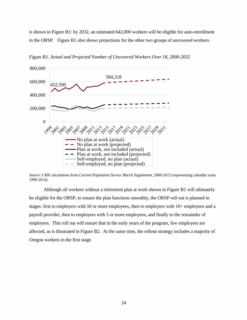
is shown in Figure B1: by 2032, an estimated 642,000 workers will be eligible for auto-enrollment
in the ORSP. Figure B1 also shows projections for the other two groups of uncovered workers.
Figure B1. Actual and Projected Number of Uncovered Workers Over 18, 2000-2032
Source: CRR calculations from Current Population Survey March Supplement, 2000-2015 (representing calendar years
1999-2014).
Although all workers without a retirement plan at work shown in Figure B1 will ultimately
be eligible for the ORSP, to ensure the plan functions smoothly, the ORSP roll out is planned in
stages: first to employers with 50 or more employees, then to employers with 10+ employees and a
payroll provider, then to employers with 5 or more employees, and finally to the remainder of
employers. This roll out will ensure that in the early years of the program, few employers are
affected, as is illustrated in Figure B2. At the same time, the rollout strategy includes a majority of
Oregon workers in the first stage.
452,590
584,318
0
200,000
400,000
600,000
800,000
No plan at work (actual)No plan at work (projected)Plan at work, not included (actual)Plan at work, not included (projected)Self-employed, no plan (actual)Self-employed, no plan (projected)

25
Figure B2. Share of Employers and Employees by Size and Payroll Management
Sources: Oregon Employment Division, 2015; and Current Population Survey March Supplement, 2015 (representing
calendar year 2014).
Once the number of workers without a plan at work whose employers are eligible for the
ORSP is determined, the feasibility model divides this population between those who are full-time
and those who are part-time workers. This division of workers is important for three reasons
stemming from the market research: 1) part-time workers are more likely to opt out than full-time
workers; 2) part-time workers are more mobile than full-time workers; and 3) part-time workers
earn less than full-time workers. Based on the market research, the feasibility study assumes that
roughly 75 percent of workers without a plan at work are full-time workers (30 or more hours per
week) and the remainder are part-time workers.
Of course, not all of these workers will participate in the plan. For one, employers currently
without a plan may decide they would rather offer a private-sector alternative to the ORSP. Until
the program is actually rolled out, it is unclear how often this will occur. The study has assumed
that 20 percent of employers currently not offering a plan take this alternative course and that there
is not a relationship between the number of employees at a firm and the firm deciding to offer a
private sector alternative. This combination of assumptions means that the number of potential
participants highlighted in Figure B1 is reduced by 20 percent in the study.
2.6% 6.3%
91.2%
56.2%
9.7%
34.1%
0%
20%
40%
60%
80%
100%
50+ employees 10+ employees w/
payroll provider
(But not 50+
employees)
Other employers
Share of employers
Share of employees

26
Next, some workers who are eligible for the plan and whose employer chooses the ORSP
will opt out. Under the plan design currently being considered – a Roth IRA with a default
contribution of 5 percent, auto-escalating to 10 percent – the Center for Retirement Research (CRR)
estimates that roughly 79 percent of full-time and 76 percent of part-time workers will participate in
the program. This estimate is based on a nationwide survey of uncovered workers, with the results
weighted to reflect the Oregon population distribution of income and age.12
These participation
rates reflect the fact that auto-escalation is predicted to decrease the probability of participation by
about 5 percentage points. The rates also reflect the age and income distribution of Oregon workers
– older workers are less likely to participate in the ORSP and higher-income workers are more
likely to participate. Although other relevant variables do influence participation – for example,
Hispanic and black workers are more likely to participate than whites – the most significant are
income and age. Because these participation rates are estimates, the feasibility model is also tested
under lower assumed rates of participation, with results presented in the main body of the report.
The number of “active accounts’ is arrived at by multiplying the number of eligible workers
and the participation – i.e., the number of accounts where an individual is currently contributing
from their paycheck. Based on the estimates contained in Figures B1 and B2 and the participation
rates discussed above, Figure B3 shows the number of full- and part-time active participants over
the first 15 years of the plan. Participation quickly increases during the first three years of the
program as more employers are reached by the roll-out and then continues to grow in line with
population growth.
12 See the Market Research Report for more detail on how these estimates were maintained.

27
Figure B3. Estimated Number of Full- and Part-time Active Participants
Source: CRR calculations.
Number of Inactive Participants
Inactive participants are participants formerly eligible and participating in the ORSP but
who have either become unemployed or switched to a job not covered by the ORSP (because the
employer offers a qualified plan), but maintained their account. Three factors influence the number
of inactive accounts. The first is the level of job-to-job and job-to-nonemployment mobility
amongst active participants. The second is the rate at which participants who switch jobs end up
employed at an employer offering a qualified plan. The third is the rate at which workers making
these transitions close their accounts.
To estimate the first two quantities, longitudinal data are required to follow individual
workers who would currently be eligible for ORSP to see their transition rates. For this purpose, the
Current Population Survey used throughout much of this study is inadequate, since it contains the
required longitudinal data for only a subset of its sample. Instead, the study turns to the Survey of
Income and Program Participation, a study that follows individuals for two to five years and asks
detailed information about retirement plans and tracks an individual’s place of employment. In
particular, the study identifies a sample of workers who would be eligible for ORSP and then
follows them for 1 year to see if they: 1) remain at the same job; 2) switch jobs; 3) become
0
100,000
200,000
300,000
400,000
1 2 3 4 5 6 7 8 9 10 11 12 13 14 15
Plan year
Full-time active participants
Part-time active participants

28
nonemployed; or 4) exit the state of Oregon. The study assumes workers who switch jobs or
become non-employed have the chance to become inactive participants, while workers exiting the
state will close their accounts (see below). Table B2 shows the estimated rates of mobility obtained.
Table B2. One-Year Job Mobility Rates for Oregon and U.S. Workers by Coverage and Hours
Worked, 1997, 2005, and 2009
Full-time Part-time
Covered at
work
Employer does
not offer plan
Employer
offers plan,
not included
Covered at
work
Employer does
not offer plan
Employer
offers plan,
not included
I. Oregon
Same employer 82.2 % 62.7 % 59.3 % 81.5 % 56.1 % 46.2 %
New employer 11.2 23.1 28.8 11.1 26.3 30.8
Not working 5.1 11.8 8.5 7.4 15.8 23.1
Exit Oregon 1.5 2.4 3.4 0.0 1.8 0.0
II. Rest of U.S.
Same employer 79.9 67.7 65.0 68.3 53.4 53.9
New employer 14.8 23.1 26.4 21.3 28.3 30.1
Not working 3.8 7.8 6.4 8.9 16.8 13.6
Exit state 1.4 1.3 2.3 1.5 1.5 2.4
Source: Survey of Income and Program Participation, 1996, 2004, and 2008 Panels (representing data on mobility for
1997, 2005, and 2009).
Because the sample of workers from any one state in the SIPP is small, Table B2 shows the
needed results for both U.S. workers and Oregon workers. The results are fairly similar and indicate
that workers affected by ORSP are more mobile than workers covered by a plan with part-time
workers especially so. Because the sample of Oregon workers is relatively small, U.S. estimates
were used in the study. Although the table above uses several panels of the SIPP to increase sample
sizes, the 2008 data has a special feature: it asks people two different times one year apart about
their employer’s pension offerings while the other panels only ask these questions once. This
allows the study to estimate the second quantity above, the rate at which employees who switch jobs
end up at an employer offering a qualified plan. This was accomplished by examining the pension
coverage of workers who were not covered by a plan in 2009 when they were first interviewed
about retirement plans, but who said they were covered in 2010. The study finds that 74 percent of
eligible workers who switched jobs still did not have a retirement savings plan at their second job.

29
These numbers can be used to estimate the rate at which workers either remain covered by
ORSP or transition out of the program. Because 68 percent of eligible workers remain at the same
job and another 17 percent (0.23*0.74) switch jobs but remain eligible for ORSP, the study assumes
85 percent of active accounts remain active.13
Of the remaining 15 percent, 6 percent of workers are
assumed to switch jobs to employers ineligible for the ORSP. Of these, and in the absence of
reliable data on the likely rate account closures, the study assumes 20 percent close their account
and 80 percent maintain it. An additional 8 percent of workers are assumed to leave their job for
nonemployment. Of these, we assume 30 percent retire (based on the age profile of Oregon
workers), while 70 percent look for work and have a choice as to whether to maintain their account.
Again, we assume 20 percent of these workers close their accounts while 80 percent maintain them.
The net result of these assumptions is that in any period, about 5 percent (0.23*0.26*0.80) become
inactive due to switching to an ineligible employer while 4 percent (0.08*0.70*0.80) of active
accounts will become inactive due to nonemployment.14
The end result is shown in Figure B4.
13 This number is for full-time workers. Part-time workers have a rate of 74 percent remaining active, which is lower
than for full-time workers due to part-time workers higher rates of job mobility and transitions to not working. 14
This number is for full-time workers. Part-time workers have a rate of 15 percent becoming inactive, which is higher
than for full-time workers due to part-time workers higher rates of job mobility and transitions to not working.

30
Figure B4. Estimated Number of Full- and Part-time Inactive Participants
Source: CRR calculations.
Account Closures
Workers who transition to an ineligible employer or who cease working temporarily can
also close their accounts. The numbers presented above can be used to calculate the rate of account
closures in a straightforward way. Because 20 percent of workers who move to an ineligible
employer close their accounts, a little over 1 percent (0.06*0.20) of active accounts will be closed
by these workers. Another 1 percent (0.08*0.70*0.20) will be closed by workers who cease
working temporarily. Finally, we assume all workers retiring or leaving the state of Oregon close
their accounts. This results in an additional 4 percent of active accounts closing – 2 percent due to
retirement (0.080*0.30) and 2 percent due to moving out of Oregon. On the whole, about 6 percent
of active accounts are assumed to close each year.15
15 This is the number for full-time workers. Part-time workers have a rate of 10 percent closing, which is higher than for
full-time workers due to part-time workers higher rates of job mobility and transitions to not working.
0
20,000
40,000
60,000
80,000
100,000
120,000
1 2 3 4 5 6 7 8 9 10 11 12 13 14 15
Plan year
Full-time inactive participantsPart-time inactive participants
31
Inactive Accounts Returning to Active
The last transitional feature of the model is that some inactive accounts become active. In
particular, the model assumes that all unemployed workers “churn” back into the market the next
year, since typically spells of not working are brief. Of inactive accounts held by workers at
ineligible employers, a small fraction re-enter the ORSP each year as they transition back to the
covered sector. In the Survey of Income and Program Participation analysis described above, about
11 percent of workers with a plan at work switch jobs in a given year and, of these, about 33 percent
switch to a job without a plan. Thus, each year about 4 percent of inactive accounts held by workers
outside of ORSP reenter the program.