Fast spatio-temporal stereo for intelligent transportation systems

INDUSTRIAL AND COMMERCIAL APPLICATION

Fast spatio-temporal stereo for intelligent transportation systems

Abdenbi Mazoul • Mohamed El Ansari •

Khalid Zebbara • George Bebis

Received: 16 September 2011 / Accepted: 12 November 2012 / Published online: 7 December 2012

� Springer-Verlag London 2012

Abstract This paper presents a fast approach for match-

ing stereoscopic images acquired by stereo cameras

mounted aboard a moving car. The proposed approach

exploits the spatio-temporal consistency between consecu-

tive frames in stereo sequences to improve matching results.

This means that the matching process at current frame uses

the matching results obtained at its preceding one. The

preceding frame allows to compute an Initial Disparity Map

for the current frame. The initial disparity map is used to

derive disparity ranges for each scanline as well as what we

call Matching Control Edge Points. Dynamic programming

is performed for matching edge points in stereo pairs. The

matching control edge points are used to drive the search for

an optimal solution in the search plane. This is accom-

plished by dividing the dynamic programming search space

into a number of subspaces depending on the number of the

matching control edge points. The proposed approach has

been tested both on virtual and real stereo images sequences

demonstrating satisfactory performance.

Keywords Stereo matching � Stereo sequences �Spatio-temporal matching � Intelligent transportation

systems

1 Introduction

Stereo vision [2] is a well-known method for obtaining an

accurate and detailed 3D representation of the environment

around an intelligent vehicle (IV). The key problem in

stereo vision is finding correspondences between pixels of

stereo images taken from different viewpoints [1].

Exhaustive surveys on methods tackling the correspon-

dence problem can be found in [4, 8]. A taxonomy of dense

stereo correspondence algorithms together with a testbed

for quantitative evaluation of stereo algorithms is provided

by Scharstein and Szeliski [18]. According to the taxon-

omy, graph-cuts-based methods [3] seem to outperform

other methods, but they are time consuming which makes

them not suitable for real-time applications (e.g., advanced

driver assistance systems (ADAS).

Although there is strong support that incorporating

temporal information in stereo matching can achieve better

results [7, 9, 12, 22], only a small amount of research has

been devoted to the reconstruction of dynamic scenes from

stereo images sequences. We believe that by considering

the temporal consistency between consecutive frames,

stereo matching results could be improved [10, 11]. This

paper presents a new stereo matching method which

exploits the similarity of edge curves in consecutive stereo

pairs of images captured by a stereo camera mounted

aboard an IV. The proposed method represents an exten-

sion of the one presented in [10]. Using temporal infor-

mation, the key question is ‘‘how to match stereo images in

the current frame using the matching results from the

A. Mazoul � M. El Ansari (&) � K. Zebbara

LabSIV, Department of Computer Science, Faculty of Science,

Ibn Zohr University, BP 8106, 80000 Agadir, Morocco

e-mail: [email protected]; [email protected]

M. El Ansari

LITIS EA 4108, INSA de Rouen, Avenue de l’Universite,

BP 8, 76801 Saint-Etienne-du-Rouvray Cedex, France

G. Bebis

CVL Laboratory, Department of Computer Science

and Engineering, University of Nevada, Reno, NV 89557, USA

G. Bebis

Computer Science Department, King Saud University,

Riyadh, Saudi Arabia

123

Pattern Anal Applic (2014) 17:211–221

DOI 10.1007/s10044-012-0310-x

preceding frame?’’. In addressing the above question, first

we have to think how to determine a link between the

current and preceding frames. Here, we use the approach

detailed in [10].

Specifically, edge points are extracted and significant

edge curves are selected in consecutive stereo image pairs.

The spatial correspondences between the curves of the

preceding frame are deduced from the pairs of matched

edge points in the same frame. Temporal matching of the

curves of the left and right consecutive images are com-

puted based on the so-called ‘‘association’’ [10]. As a

result, the spatial correspondences between the curves in

the current frame are inferred. Matched edge points,

belonging to the matched curves, are used as control points

to drive the dynamic programming search process [17] for

matching all edge points in the current stereo pair. The

proposed method has been tested on both virtual and real

stereo images sequences showing satisfactory performance.

The rest of the paper is organized as follows. Section 2

overviews stereo methods handling stereo sequences and

employing temporal consistency. The proposed stereo

method is detailed in Sect. 3 Our experimental results and

comparisons are presented in Sect. 4 Finally, Sect. 5 con-

cludes the paper.

2 Related work

In recent years, several techniques have been proposed to

obtain more accurate disparity maps from stereo sequences

by utilizing temporal consistency [7, 12, 20, 22]. Most of

these methods use either optical flow or a spatio-temporal

window for matching stereo sequences. In Tao et al. [20], a

dynamic depth recovery approach was proposed to incre-

mentally obtain a scene representation, consisting of

piecewise planar surface patches. Their method employs

color segmentation and models each segment as a 3D

plane. The motion of a plane is described using constant

velocity. A spatial match measure and a scene flow con-

straint [21] are employed in the matching process. The

processing speed of the method and the accuracy of the

results presented are limited by the image segmentation

algorithm used.

Vedula et al. [21] presented a linear algorithm to com-

pute 3D scene flow from 2D optical flow and estimate 3D

structure information from scene flow. In [14], the tem-

poral consistency was enforced by minimizing the differ-

ence between the disparity maps of consecutive frames.

That approach was designed for off-line processing only

(i.e. it takes pre-captured stereo sequences as input and

calculates the disparity maps for all frames at the same

time). In [12], an algorithm was developed to compute both

disparity maps and disparity flow maps in an integrated

way. The disparity map generated for the current frame is

used to predict the disparity map for the next frame. The

estimated disparity map provides spatial correspondence

information which was used to cross-validate the disparity

flow maps estimated for different views. Programmable

graphics hardware was used for speeding up processing.

Zhang et al. [22], extended traditional methods by using

both spatial and temporal information. The spatial window

typically used to compute the sum of squared differences

(SSD) cost function was extended to a spatio-temporal

window for computing the sum of SSD (SSSD). Their

method could improve results when dealing with static

scenes and structured light. However, it fails to do so when

dealing with dynamic scenes. Davis et al. [7] have devel-

oped a similar framework as in [22]. However, their work

was focused on geometrically static scenes imaged under

varying illumination. Given an input sequence taken by a

freely moving camera, Zhang et al. [23] proposed a novel

approach to construct a view-dependent depth map for each

frame. The method takes a sequence as input and provides

the depth for different frame. That approach was also

designed for off-line processing, so it is not applicable in

an IV.

Recently, the so-called ‘‘association’’ was presented as a

technique to find a relationship between consecutive stereo

pairs [10]. Using the same technique to obtain a link

between adjacent frames, we proposed a spatio-temporal

approach to match edge curves in adjacent frames. The

edge points of the matched edge curves form a set of

control points which are used to drive dynamic program-

ming during matching.

3 Stereo matching algorithm

In this section, we describe the steps of the proposed

method for matching stereo images captured by a stereo

sensor mounted aboard an IV. It should be noted that the

stereoscopic sensor used in our experiments provides

rectified images (i.e., corresponding pixels have the same

y-coordinate). The key idea of the proposed approach is

exploiting the link between consecutive stereo pairs. In this

sense, the matching results from the preceding stereo pair

are used to obtain matching results in the current stereo

pair. The following notation will be used in the rest of the

paper: Ik-1L and Ik-1

R denote the left and right stereo images

of frame fk-1, acquired at time k - 1, and dk-1 is the

corresponding disparity map. IkL and Ik

R represent the left

and right stereo images of frame fk, acquired at time k. We

assume that frame fk = (IkL, Ik

R) represents the current ste-

reo pair for which we want to compute the disparity map

dk. fk-1 = (Ik-1L ,Ik-1

R ) represents the preceding frame for

which the disparity map dk-1 is available. The matching

212 Pattern Anal Applic (2014) 17:211–221

123

problem is formulated as follows: compute dk by taking

into account dk-1 and the relationship between frames fk-1

and fk. A summary of processing steps of the proposed

method is given in Fig. 1.

3.1 Edge detection

The first step consists of extracting significant features

from the stereo images to be matched. Here, we are

interested in employing edge points for matching. In [10],

the declivity operator [16] was used to detect edge points

from stereo sequences. This operator, however, is not able

to detect horizontal edge curves. Therefore, it misses an

interesting number of edge points and the resulting

disparity map is rather sparse. In this work, we use the

Canny edge detector [5] which provides continuous edge

curves, which are vital to the proposed matching method.

Using the Canny detector yields more edge points, leading

to richer 3D information. The following notation is

used throughout the paper: Smf ¼ C

m;if

n oi¼1;...;Nm

f

denotes

the set of edge curves extracted from image Ifm where

f 2 fk � 1; kg represents the frame index and m 2 fL;Rgrepresents the index of the stereo image, (i.e. L for left

image and R for right image). Nfm represents the number of

edge curves in Ifm.

3.2 Association between edge points in consecutive

images

As mentioned earlier, the main idea of the proposed

approach is exploiting the relationship between consecu-

tive stereo pairs. The so-called association technique, for

achieving this task, was proposed in [10]. In this subsec-

tion, we review the method used to find the association

between edge points in consecutive frames [i.e., the asso-

ciation between edge points in the images Ik-1L and Ik

L (resp.

Ik-1R and Ik

R)].

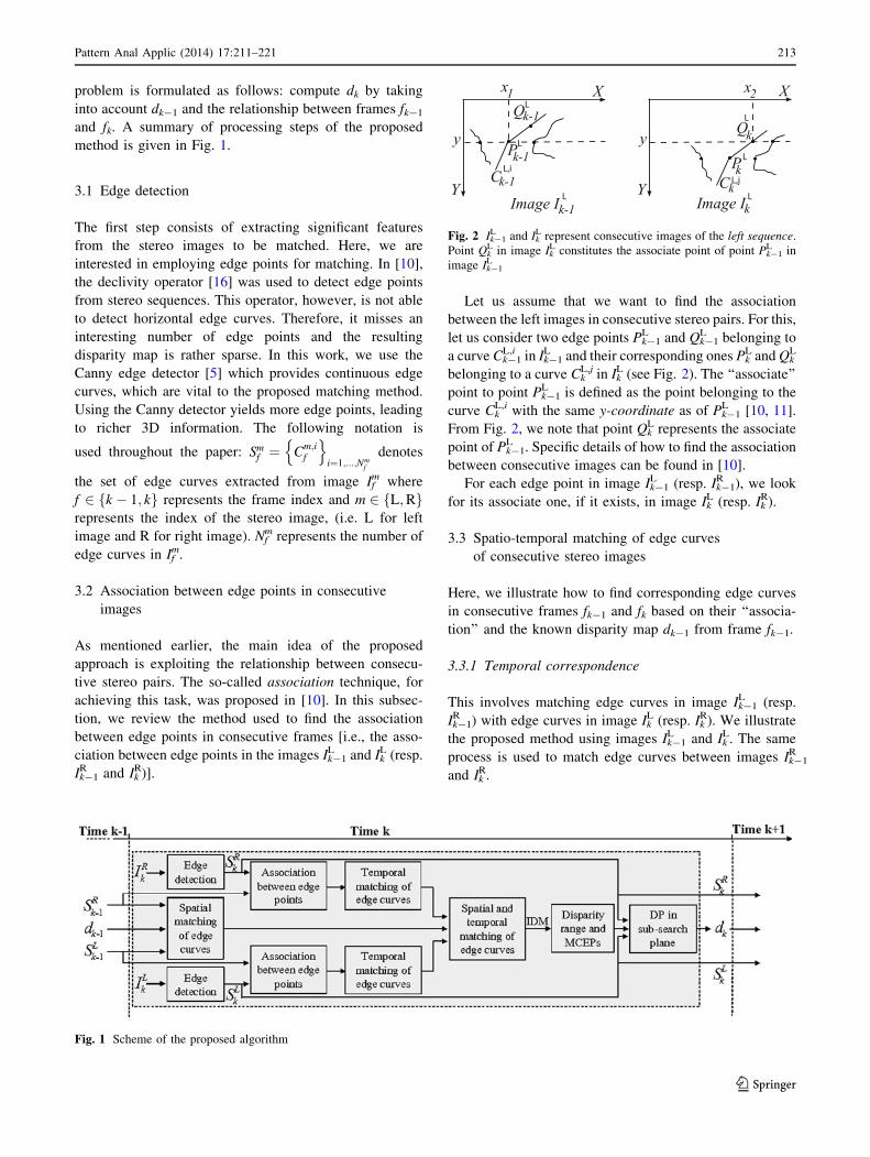
Let us assume that we want to find the association

between the left images in consecutive stereo pairs. For this,

let us consider two edge points Pk-1L and Qk-1

L belonging to

a curve Ck-1L,i in Ik-1

L and their corresponding ones PkL and Qk

L

belonging to a curve CkL,j in Ik

L (see Fig. 2). The ‘‘associate’’

point to point Pk-1L is defined as the point belonging to the

curve CkL,i with the same y-coordinate as of Pk-1

L [10, 11].

From Fig. 2, we note that point QkL represents the associate

point of Pk-1L . Specific details of how to find the association

between consecutive images can be found in [10].

For each edge point in image Ik-1L (resp. Ik-1

R ), we look

for its associate one, if it exists, in image IkL (resp. Ik

R).

3.3 Spatio-temporal matching of edge curves

of consecutive stereo images

Here, we illustrate how to find corresponding edge curves

in consecutive frames fk-1 and fk based on their ‘‘associa-

tion’’ and the known disparity map dk-1 from frame fk-1.

3.3.1 Temporal correspondence

This involves matching edge curves in image Ik-1L (resp.

Ik-1R ) with edge curves in image Ik

L (resp. IkR). We illustrate

the proposed method using images Ik-1L and Ik

L. The same

process is used to match edge curves between images Ik-1R

and IkR.

Fig. 1 Scheme of the proposed algorithm

Fig. 2 Ik-1L and Ik

L represent consecutive images of the left sequence.

Point QkL in image Ik

L constitutes the associate point of point Pk-1L in

image Ik-1L

Pattern Anal Applic (2014) 17:211–221 213

123

Temporal correspondence consists of finding for each

edge curve Ck-1L,i in the set Sk-1

L its corresponding edge

curve CkL,j in the set Sk

L, if it exists. Let AssðCL;ik�1Þ ¼

aenf gn¼1;...;Nibe the set of edge points aen, belonging to

image IkL, which represent the associates of the edge points

of edge curve Ck-1L,i . Ni is the number of associations found

for the edge curve Ck-1L,i . If Mi represents the number of

edge points in Ck-1L,i , Ni B Mi because there are edge points

in image Ik-1L with no associates in image Ik

L. If the asso-

ciation process is error-free, all the edge points belonging

to the set Ass(Ck-1L,i ) should belong to the same edge curve,

which is the curve corresponding to Ck-1L,i . Unfortunately,

there might be some errors inherent to the association

process. Consequently, the edge points aem may belong to

different curves in SkL. We find the match of Ck-1

L,i by

looking for the curve CkL,j, which contains the maximum

number of edge points in Ass(Ck-1L,i ). We apply the same

method to all the edge curves in Sk-1L to find their corre-

sponding ones in SkL.

3.3.2 Spatial correspondence

This step involves matching the edge curves between the

stereo images Ik-1L and Ik-1

R using the disparity map dk-1.

The same principle, as in the case of establishing the

temporal correspondences, is used to find the spatial

correspondences.

Let MatchðCL;ik�1Þ ¼ menf gn¼1;...;Ni

be the set of edge

points men, belonging to the image Ik-1R , which match the

edge points of Ck-1L,i . Ni is the number of matched edge

points belonging to Ck-1L,i . If Mi represents the number of

edge points in Ck-1L,i , Ni B Mi because there is a number of

edge points in image Ik-1L for which there is no match in

image Ik-1R . If there is no error in the matching process, all

edge points belonging to the set Match(Ck-1L,i ) should

belong to a single edge curve, which is the corresponding

of the curve Ck-1L,i . Unfortunately again, there might be

some errors inherent to the matching process. Conse-

quently, the edge points mem may belong to different

curves in Sk-1R . We find the match of the curve Ck-1

L,i by

looking for the curve Ck-1R,j , which contains the maximum

number of edge points in Match(Ck-1L,i ).

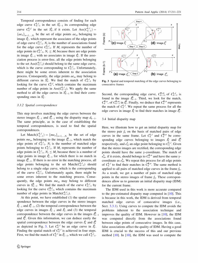
At this point, we have established (1) the spatial corre-

spondence between the edge curves in the stereo images

Ik-1L and Ik-1

R , (2) the temporal correspondence between the

edge curves in images Ik-1L and Ik

L, and (3) the temporal

correspondence between the edge curves in the images Ik-1R

and IkR. Given this information, we can deduce easily the

spatial correspondence between the edge curves IkL and Ik

R

as depicted in Fig. 3. Let CkL,i be an edge curve in Ik

L.

Finding the spatial match of CkL,i is achieved in four steps.

First, we find the match of CkL,i in Ik-1

L , which we call Ck-1L,j .

Second, the corresponding edge curve, Ck-1R,m, of Ck-1

L,j is

found in the image Ik-1R . Third, we look for the match,

CkR,n, of Ck-1

R,m in IkR. Finally, we deduce that Ck

R,n represents

the match of CkL,i. We repeat the same process for all the

edge curves in image IkL to find their matches in image Ik

R.

3.4 Initial disparity map

Here, we illustrate how to get an initial disparity map for

the stereo pair fk on the basis of matched pairs of edge

curves in the same frame. Let CkL,i and Ck

R,n be corre-

sponding edge curves belonging to images IkL and Ik

R

respectively, and emL an edge point belonging to Ck

L,i. Given

that the stereo images are rectified, the corresponding edge

points should have the same y-coordinate. The match of

emL, if it exists, should belongs to Ck

R,n and have the same y-

coordinate as emL. We repeat this process for all edge points

of CkL,i to find their matches in Ck

R,n. The same method is

applied to all pairs of matched edge curves in the frame fk.

As a result, we get a number of pairs of matched edge

points in the stereo images of frame fk. These correspon-

dences allow us to generate an initial disparity map (IDM)

for the current frame.

The IDM used in this work is more accurate compared

to the pre-estimated disparity map computed in [10]. This

is because in this work, the IDM is derived from temporal

matched edge curves of consecutive images (i.e.,

Sect. 3.3.1). Using curves to compute the IDM avoids the

problems inherent to the association technique and

improves the quality of IDM. However in [10], the IDM

was computed directly from the associations found

between edge points of consecutive images. In this case,

false associations affect the quality of IDM. Having a good

IDM is crucial to the success of this and our previous

method [10]. In [10], the IDM was used to compute the

Fig. 3 Spatial and temporal matching of the edge curves belonging to

consecutive frames


123

disparity range. Here, it is being used to estimate the dis-

parity range as well as obtain the matched control edge

points (MCEPs) which drive the dynamic programming for

matching the remaining edge points in the current frame

(i.e., Sect. 3.5.3)

3.5 Stereo matching method of edge points

of the current frame

In Sect. 3.4, we described how to match the edge points

belonging to the edge curves in frame fk. This section

presents our method for matching the remaining edge

points of the current frame by considering the MCEPs.

3.5.1 Disparity range constraint

The accurate choice of the maximum disparity threshold

value is crucial to the quality of the output disparity map and

computation time [6, 18]. In [10, 11], a method to compute

the range of possible disparities was presented. The method

was based on analyzing the v-disparity [13] computed from

the IDM. This provides the disparity range for each scan-

line of the stereo images. We use the same idea here to

determine the disparity range for each image line in the

matched stereo pair. More details can be found in [10].

3.5.2 Cost function

As a similarity criterion between corresponding edge

points, we use a cost function based on the gradient mag-

nitude and orientation at the matched edge points. Let eL

and eR be two edge points belonging to images IkL and

IkR, respectively. We denote by mL and mR (resp. hL and hR)

their gradient magnitudes (resp. orientations). We assume

that corresponding edge points in stereo images should

have the same (or close) gradient magnitudes as well as the

same (or close) orientations. Therefore, we define the cost

function as follows:

CðeL; eRÞ ¼ ILk ðxL; yLÞ � IR

k ðxR; yRÞ� �2þðmLÞ2n

þ mRÞ2 � 2 � mL � mR � cosðhL � hRÞ� o1=2

ð1Þ

where (xL, yL) and (xR, yR) are the coordinates of the edge

points eL and eR, respectively.

3.5.3 Dynamic programming

Let {ei,slL }i=1,…,N_sl

L (resp. {ej,slR }j=1,…,N_sl

R ) be the set of edge

points in scan-line sl of image IkL (resp. Ik

R). We assume that

these points are ordered according to their x-coordinate; NslL

(resp. NslR) is the number of points. We demonstrate how to

match these edge points for scan-line sl using dynamic

programming. The same technique is used for all scan-lines

in the stereo images IkL and Ik

R.

The problem of obtaining correspondences between

edge points on right and left epipolar scan-lines can be

expressed as a path finding problem on the 2D plane [17].

We propose to subdivide the search space into several sub-

spaces, depending on the number of MCEPs found at scan-

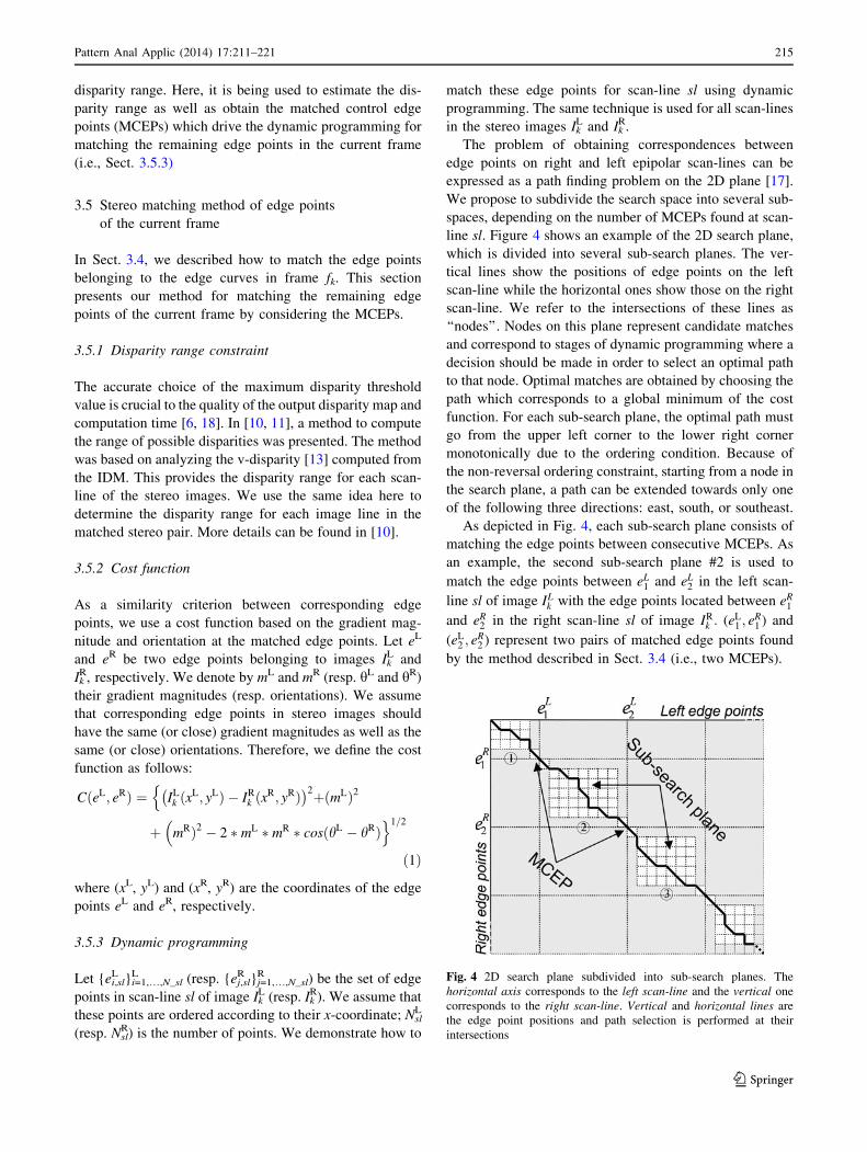
line sl. Figure 4 shows an example of the 2D search plane,

which is divided into several sub-search planes. The ver-

tical lines show the positions of edge points on the left

scan-line while the horizontal ones show those on the right

scan-line. We refer to the intersections of these lines as

‘‘nodes’’. Nodes on this plane represent candidate matches

and correspond to stages of dynamic programming where a

decision should be made in order to select an optimal path

to that node. Optimal matches are obtained by choosing the

path which corresponds to a global minimum of the cost

function. For each sub-search plane, the optimal path must

go from the upper left corner to the lower right corner

monotonically due to the ordering condition. Because of

the non-reversal ordering constraint, starting from a node in

the search plane, a path can be extended towards only one

of the following three directions: east, south, or southeast.

As depicted in Fig. 4, each sub-search plane consists of

matching the edge points between consecutive MCEPs. As

an example, the second sub-search plane #2 is used to

match the edge points between eL1 and eL

2 in the left scan-

line sl of image ILk with the edge points located between eR

1

and eR2 in the right scan-line sl of image IR

k : (eL1 ; e

R1 ) and

(eL2 ; e

R2 ) represent two pairs of matched edge points found

by the method described in Sect. 3.4 (i.e., two MCEPs).

Fig. 4 2D search plane subdivided into sub-search planes. The

horizontal axis corresponds to the left scan-line and the vertical one

corresponds to the right scan-line. Vertical and horizontal lines are

the edge point positions and path selection is performed at their

intersections


123

First, the disparity range is used to select the valid nodes

for the sub-search plane #2. Second, the cost function

(Eq. 1) is used to find additional matches between the valid

nodes. After the optimal path has been found, the pairs of

corresponding edge points between eL1 and eL

2 in the left

scan-line and those between eR1 and eR

2 in the right scan-line

are determined. The same process is repeated for all the

sub-search planes. The same method is applied to all other

scan-lines for matching the edge points of the whole image.

As we detailed above, for each scan-line the dynamic

programming space is divided into a number of subspaces

depending on the number of MCEPs found. We are con-

fident of the correctness of the matched edge points used as

MCEPs. MCEPs force the dynamic programming search

process to follow the correct path. Therefore, the proposed

method provides less mismatches than our previous method

reported in [10] which uses a single search space only.

3.6 Algorithm of the proposed method

The algorithm of the proposed matching approach can be

described as follows:

4 Experimental results

To evaluate the performance of the proposed approach, we

experimented with different stereo sequences. Let us refer

to the new method as Spatio-Temporal Matching (STM)

method. The STM method is developed based on the TCM

(Temporal Consistent Matching) method [10]. Comparison

results between the two methods are presented to show the

improvements brought by STM.

4.1 Virtual stereo image sequences

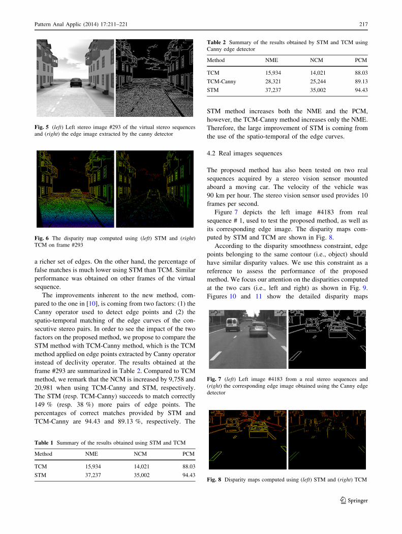
First, we used the MARS/PRESCAN virtual stereo images

available from [19]. The size of the images is 512 9 512.

The left stereo image of frame #293 of the virtual stereo

sequences is shown on the left side of Fig. 5. The edge

image, obtained by the Canny edge detector, is shown on

the right side of Fig. 5. The corresponding disparity maps

computed by STM and TCM are shown in Fig. 6. For

clarity, we use false colors for represent the disparity map.

Table 1 summarizes the matching results obtained from the

two methods. It shows the number of matched edge points

(NME), the number of correct matches (NCM), and the

percentage of correct matches (PCM) obtained for frame

#293. It is clear that STM yields more correct matches

compared to TCM (i.e., almost twice as many). Of course

this is due to using the Canny edge detector which provides


123

a richer set of edges. On the other hand, the percentage of

false matches is much lower using STM than TCM. Similar

performance was obtained on other frames of the virtual

sequence.

The improvements inherent to the new method, com-

pared to the one in [10], is coming from two factors: (1) the

Canny operator used to detect edge points and (2) the

spatio-temporal matching of the edge curves of the con-

secutive stereo pairs. In order to see the impact of the two

factors on the proposed method, we propose to compare the

STM method with TCM-Canny method, which is the TCM

method applied on edge points extracted by Canny operator

instead of declivity operator. The results obtained at the

frame #293 are summarized in Table 2. Compared to TCM

method, we remark that the NCM is increased by 9,758 and

20,981 when using TCM-Canny and STM, respectively.

The STM (resp. TCM-Canny) succeeds to match correctly

149 % (resp. 38 %) more pairs of edge points. The

percentages of correct matches provided by STM and

TCM-Canny are 94.43 and 89.13 %, respectively. The

STM method increases both the NME and the PCM,

however, the TCM-Canny method increases only the NME.

Therefore, the large improvement of STM is coming from

the use of the spatio-temporal of the edge curves.

4.2 Real images sequences

The proposed method has also been tested on two real

sequences acquired by a stereo vision sensor mounted

aboard a moving car. The velocity of the vehicle was

90 km per hour. The stereo vision sensor used provides 10

frames per second.

Figure 7 depicts the left image #4183 from real

sequence # 1, used to test the proposed method, as well as

its corresponding edge image. The disparity maps com-

puted by STM and TCM are shown in Fig. 8.

According to the disparity smoothness constraint, edge

points belonging to the same contour (i.e., object) should

have similar disparity values. We use this constraint as a

reference to assess the performance of the proposed

method. We focus our attention on the disparities computed

at the two cars (i.e., left and right) as shown in Fig. 9.

Figures 10 and 11 show the detailed disparity maps

Fig. 5 (left) Left stereo image #293 of the virtual stereo sequences

and (right) the edge image extracted by the canny detector

Fig. 6 The disparity map computed using (left) STM and (right)

TCM on frame #293

Table 1 Summary of the results obtained using STM and TCM

Method NME NCM PCM

TCM 15,934 14,021 88.03

STM 37,237 35,002 94.43

Table 2 Summary of the results obtained by STM and TCM using

Canny edge detector

Method NME NCM PCM

TCM 15,934 14,021 88.03

TCM-Canny 28,321 25,244 89.13

STM 37,237 35,002 94.43

Fig. 7 (left) Left image #4183 from a real stereo sequences and

(right) the corresponding edge image obtained using the Canny edge

detector

Fig. 8 Disparity maps computed using (left) STM and (right) TCM


123

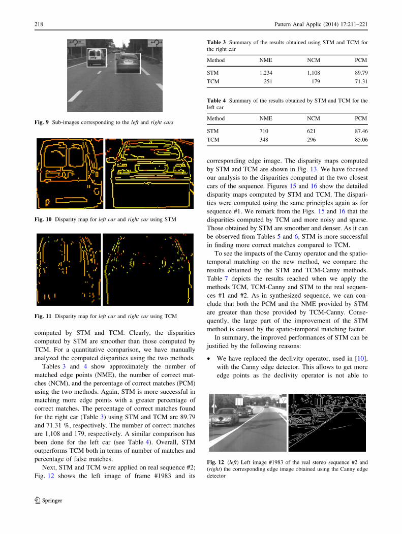
computed by STM and TCM. Clearly, the disparities

computed by STM are smoother than those computed by

TCM. For a quantitative comparison, we have manually

analyzed the computed disparities using the two methods.

Tables 3 and 4 show approximately the number of

matched edge points (NME), the number of correct mat-

ches (NCM), and the percentage of correct matches (PCM)

using the two methods. Again, STM is more successful in

matching more edge points with a greater percentage of

correct matches. The percentage of correct matches found

for the right car (Table 3) using STM and TCM are 89.79

and 71.31 %, respectively. The number of correct matches

are 1,108 and 179, respectively. A similar comparison has

been done for the left car (see Table 4). Overall, STM

outperforms TCM both in terms of number of matches and

percentage of false matches.

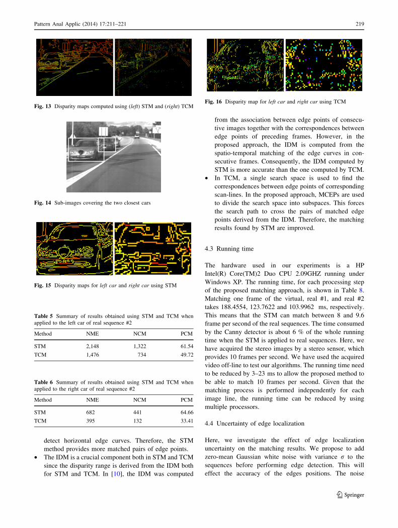
Next, STM and TCM were applied on real sequence #2;

Fig. 12 shows the left image of frame #1983 and its

corresponding edge image. The disparity maps computed

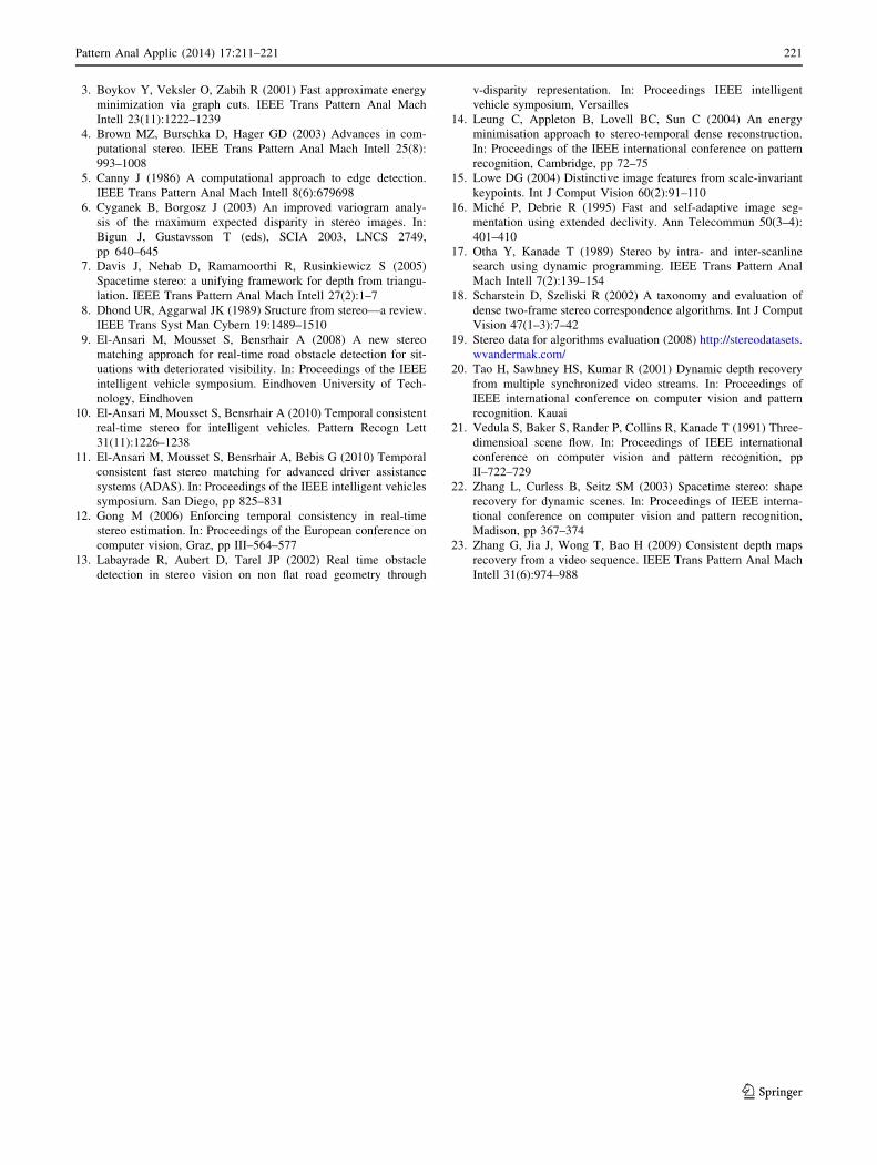
by STM and TCM are shown in Fig. 13. We have focused

our analysis to the disparities computed at the two closest

cars of the sequence. Figures 15 and 16 show the detailed

disparity maps computed by STM and TCM. The dispari-

ties were computed using the same principles again as for

sequence #1. We remark from the Figs. 15 and 16 that the

disparities computed by TCM and more noisy and sparse.

Those obtained by STM are smoother and denser. As it can

be observed from Tables 5 and 6, STM is more successful

in finding more correct matches compared to TCM.

To see the impacts of the Canny operator and the spatio-

temporal matching on the new method, we compare the

results obtained by the STM and TCM-Canny methods.

Table 7 depicts the results reached when we apply the

methods TCM, TCM-Canny and STM to the real sequen-

ces #1 and #2. As in synthesized sequence, we can con-

clude that both the PCM and the NME provided by STM

are greater than those provided by TCM-Canny. Conse-

quently, the large part of the improvement of the STM

method is caused by the spatio-temporal matching factor.

In summary, the improved performances of STM can be

justified by the following reasons:

• We have replaced the declivity operator, used in [10],

with the Canny edge detector. This allows to get more

edge points as the declivity operator is not able to

Fig. 9 Sub-images corresponding to the left and right cars

Fig. 10 Disparity map for left car and right car using STM

Fig. 11 Disparity map for left car and right car using TCM

Table 3 Summary of the results obtained using STM and TCM for

the right car

Method NME NCM PCM

STM 1,234 1,108 89.79

TCM 251 179 71.31

Table 4 Summary of the results obtained by STM and TCM for the

left car

Method NME NCM PCM

STM 710 621 87.46

TCM 348 296 85.06

Fig. 12 (left) Left image #1983 of the real stereo sequence #2 and

(right) the corresponding edge image obtained using the Canny edge

detector


123

detect horizontal edge curves. Therefore, the STM

method provides more matched pairs of edge points.

• The IDM is a crucial component both in STM and TCM

since the disparity range is derived from the IDM both

for STM and TCM. In [10], the IDM was computed

from the association between edge points of consecu-

tive images together with the correspondences between

edge points of preceding frames. However, in the

proposed approach, the IDM is computed from the

spatio-temporal matching of the edge curves in con-

secutive frames. Consequently, the IDM computed by

STM is more accurate than the one computed by TCM.

• In TCM, a single search space is used to find the

correspondences between edge points of corresponding

scan-lines. In the proposed approach, MCEPs are used

to divide the search space into subspaces. This forces

the search path to cross the pairs of matched edge

points derived from the IDM. Therefore, the matching

results found by STM are improved.

4.3 Running time

The hardware used in our experiments is a HP

Intel(R) Core(TM)2 Duo CPU 2.09GHZ running under

Windows XP. The running time, for each processing step

of the proposed matching approach, is shown in Table 8.

Matching one frame of the virtual, real #1, and real #2

takes 188.4554, 123.7622 and 103.9962 ms, respectively.

This means that the STM can match between 8 and 9.6

frame per second of the real sequences. The time consumed

by the Canny detector is about 6 % of the whole running

time when the STM is applied to real sequences. Here, we

have acquired the stereo images by a stereo sensor, which

provides 10 frames per second. We have used the acquired

video off-line to test our algorithms. The running time need

to be reduced by 3–23 ms to allow the proposed method to

be able to match 10 frames per second. Given that the

matching process is performed independently for each

image line, the running time can be reduced by using

multiple processors.

4.4 Uncertainty of edge localization

Here, we investigate the effect of edge localization

uncertainty on the matching results. We propose to add

zero-mean Gaussian white noise with variance r to the

sequences before performing edge detection. This will

effect the accuracy of the edges positions. The noise

Fig. 13 Disparity maps computed using (left) STM and (right) TCM

Fig. 14 Sub-images covering the two closest cars

Fig. 15 Disparity maps for left car and right car using STM

Fig. 16 Disparity map for left car and right car using TCM

Table 5 Summary of results obtained using STM and TCM when

applied to the left car of real sequence #2

Method NME NCM PCM

STM 2,148 1,322 61.54

TCM 1,476 734 49.72

Table 6 Summary of results obtained using STM and TCM when

applied to the right car of real sequence #2

Method NME NCM PCM

STM 682 441 64.66

TCM 395 132 33.41


123

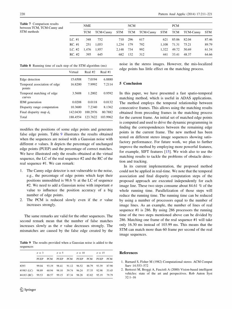
modifies the positions of some edge points and generates

false edge points. Table 9 illustrates the results obtained

when the sequences are noised with a Gaussian noise with

different r values. It depicts the percentage of unchanged

edge points (PUEP) and the percentage of correct matches.

We have illustrated only the results obtained at the virtual

sequence, the LC of the real sequence #2 and the RC of the

real sequence #1. We can remark:

1. The Canny edge detector is not vulnerable to the noise,

e.g., the percentage of edge points which kept their

positions unmodified is 98.6 % at the LC of sequence

#2. We need to add a Gaussian noise with important rvalue to influence the position accuracy of a big

number of edge points.

2. The PCM is reduced slowly even if the r value

increases strongly.

The same remarks are valid for the other sequences. The

second remark mean that the number of false matches

increases slowly as the r value decreases strongly. The

mismatches are caused by the false edge created by the

noise in the stereo images. However, the mis-localized

edge points has little effect on the matching process.

5 Conclusion

In this paper, we have presented a fast spatio-temporal

matching method, which is useful in ADAS applications.

The method employs the temporal relationship between

consecutive frames. This allows using the matching results

obtained from preceding frames in the matching process

for the current frame. An initial set of matched edge points

is computed and used to drive the dynamic programming in

finding the correspondences between the remaining edge

points in the current frame. The new method has been

tested on different stereo image sequences showing satis-

factory performance. For future work, we plan to further

improve the method by employing more powerful features,

for example, SIFT features [15]. We wish also to use the

matching results to tackle the problems of obstacle detec-

tion and tracking.

In its current implementation, the proposed method

could not be applied in real-time. We note that the temporal

association and final disparity computation steps of the

proposed approach are executed independently for each

image line. These two steps consume about 84.61 % of the

whole running time. Parallelization of those steps will

reduce the running time. The running time can be reduced

by using a number of processors equal to the number of

image lines. As an example, the number of lines of real

sequence #1 is 286. By using 286 processors the running

time of the two steps mentioned above can be divided by

286. Matching one frame of the real sequence #1 will take

only 16.30 ms instead of 103.99 ms. This means that the

STM can match more than 60 frame per second of the real

image sequences.

References

1. Barnard S, Fisher M (1982) Computational stereo. ACM Comput

Surv 14:553–572

2. Bertozzi M, Broggi A, Fascioli A (2000) Vision-based intelligent

vehicles: state of the art and perspectives. Rob Auton Syst

32:1–16

Table 7 Comparison results

between TCM, TCM-Canny and

STM methods

NME NCM PCM

TCM TCM-Canny STM TCM TCM-Canny STM TCM TCM-Canny STM

LC. #1 348 752 710 296 617 621 85.06 82.04 87.46

RC. #1 251 1,053 1,234 179 792 1,108 71.31 75.21 89.79

LC. #2 1,476 1,957 2,148 734 992 1,322 49.72 50.69 61.54

RC. #2 395 645 682 132 312 441 33.41 48.37 64.66

Table 8 Running time of each step of the STM algorithm (ms)

Virtual Real #2 Real #1

Edge detection 15.6508 7.0194 6.8880

Temporal association of edge

points

16.8200 7.9992 7.2114

Temporal matching of edge

curves

3.5608 1.2002 0.9592

IDM generation 0.0208 0.0118 0.0132

Disparity range computation 10.3600 7.2340 8.1362

Final disparity map dk 142.0430 100.2976 80.7882

Total 188.4554 123.7622 103.9962

Table 9 The results provided when a Gaussian noise is added to the

sequences

r = 3 r = 5 r = 10 r = 15

PUEP PCM PUEP PCM PUEP PCM PUEP PCM

#293 99.04 93.19 98.41 91.12 96.52 88.79 93.39 87.90

#1983 (LC) 98.89 60.94 98.10 59.74 96.24 57.35 92.98 53.45

#4183 (RC) 99.53 88.57 99.15 87.34 98.28 83.82 95.19 79.79


123

3. Boykov Y, Veksler O, Zabih R (2001) Fast approximate energy

minimization via graph cuts. IEEE Trans Pattern Anal Mach

Intell 23(11):1222–1239

4. Brown MZ, Burschka D, Hager GD (2003) Advances in com-

putational stereo. IEEE Trans Pattern Anal Mach Intell 25(8):

993–1008

5. Canny J (1986) A computational approach to edge detection.

IEEE Trans Pattern Anal Mach Intell 8(6):679698

6. Cyganek B, Borgosz J (2003) An improved variogram analy-

sis of the maximum expected disparity in stereo images. In:

Bigun J, Gustavsson T (eds), SCIA 2003, LNCS 2749,

pp 640–645

7. Davis J, Nehab D, Ramamoorthi R, Rusinkiewicz S (2005)

Spacetime stereo: a unifying framework for depth from triangu-

lation. IEEE Trans Pattern Anal Mach Intell 27(2):1–7

8. Dhond UR, Aggarwal JK (1989) Sructure from stereo—a review.

IEEE Trans Syst Man Cybern 19:1489–1510

9. El-Ansari M, Mousset S, Bensrhair A (2008) A new stereo

matching approach for real-time road obstacle detection for sit-

uations with deteriorated visibility. In: Proceedings of the IEEE

intelligent vehicle symposium. Eindhoven University of Tech-

nology, Eindhoven

10. El-Ansari M, Mousset S, Bensrhair A (2010) Temporal consistent

real-time stereo for intelligent vehicles. Pattern Recogn Lett

31(11):1226–1238

11. El-Ansari M, Mousset S, Bensrhair A, Bebis G (2010) Temporal

consistent fast stereo matching for advanced driver assistance

systems (ADAS). In: Proceedings of the IEEE intelligent vehicles

symposium. San Diego, pp 825–831

12. Gong M (2006) Enforcing temporal consistency in real-time

stereo estimation. In: Proceedings of the European conference on

computer vision, Graz, pp III–564–577

13. Labayrade R, Aubert D, Tarel JP (2002) Real time obstacle

detection in stereo vision on non flat road geometry through

v-disparity representation. In: Proceedings IEEE intelligent

vehicle symposium, Versailles

14. Leung C, Appleton B, Lovell BC, Sun C (2004) An energy

minimisation approach to stereo-temporal dense reconstruction.

In: Proceedings of the IEEE international conference on pattern

recognition, Cambridge, pp 72–75

15. Lowe DG (2004) Distinctive image features from scale-invariant

keypoints. Int J Comput Vision 60(2):91–110

16. Miche P, Debrie R (1995) Fast and self-adaptive image seg-

mentation using extended declivity. Ann Telecommun 50(3–4):

401–410

17. Otha Y, Kanade T (1989) Stereo by intra- and inter-scanline

search using dynamic programming. IEEE Trans Pattern Anal

Mach Intell 7(2):139–154

18. Scharstein D, Szeliski R (2002) A taxonomy and evaluation of

dense two-frame stereo correspondence algorithms. Int J Comput

Vision 47(1–3):7–42

19. Stereo data for algorithms evaluation (2008) http://stereodatasets.

wvandermak.com/

20. Tao H, Sawhney HS, Kumar R (2001) Dynamic depth recovery

from multiple synchronized video streams. In: Proceedings of

IEEE international conference on computer vision and pattern

recognition. Kauai

21. Vedula S, Baker S, Rander P, Collins R, Kanade T (1991) Three-

dimensioal scene flow. In: Proceedings of IEEE international

conference on computer vision and pattern recognition, pp

II–722–729

22. Zhang L, Curless B, Seitz SM (2003) Spacetime stereo: shape

recovery for dynamic scenes. In: Proceedings of IEEE interna-

tional conference on computer vision and pattern recognition,

Madison, pp 367–374

23. Zhang G, Jia J, Wong T, Bao H (2009) Consistent depth maps

recovery from a video sequence. IEEE Trans Pattern Anal Mach

Intell 31(6):974–988


123

http://stereodatasets.wvandermak.com/

http://stereodatasets.wvandermak.com/

Documents

Fast spatio-temporal stereo for intelligent transportation systems