Fast spatio-temporal image reconstruction for dynamic PET

IEEE TRANSACTIONS ON MEDICAL IMAGING, VOL. 18, NO. 3, MARCH 1999 185

Fast Spatio-Temporal Image Reconstructionfor Dynamic PET

Miles N. Wernick,* Member, IEEE, E. James Infusino, and Milos Milosevic, Student Member, IEEE

Abstract—In tomographic imaging, dynamic images are typi-cally obtained by reconstructing the frames of a time sequenceindependently, one by one. A disadvantage of this frame-by-framereconstruction approach is that it fails to account for temporalcorrelations in the signal. Ideally, one should treat the entireimage sequence as a single spatio-temporal signal. However, theresulting reconstruction task becomes computationally intensive.Fortunately, as we show in this paper, the spatio-temporal recon-struction problem can be greatly simplified by first applying atemporal Karhunen–Loeve (KL) transformation to the imagingequation. We show that if the regularization operator is chosen tobe separable into space and time components, penalized weightedleast squares reconstruction of the entire image sequence isapproximately equivalent to frame-by-frame reconstruction inthe space-KL domain. By this approach, spatio-temporal recon-struction can be achieved at reasonable computational cost. Onecan achieve further computational savings by discarding high-order KL components to avoid reconstructing them. Performanceof the method is demonstrated through statistical evaluations ofthe bias-variance tradeoff obtained by computer simulation.

Index Terms—Dynamic, PET, principal component analysis,reconstruction.

I. INTRODUCTION

I N POSITRON emission tomography (PET), as in manyother types of imaging, the use of short-exposure acquisi-

tions to obtain a time sequence of images provides temporalresolution at the expense of the signal-to-noise ratio (SNR) ineach image. For this reason, dynamic PET images can be verynoisy and the image-reconstruction problem for time-sequenceimages can be a challenging one.

Conventionally, a time sequence of tomographic imagesis obtained by reconstructing each image independently. Asignificant disadvantage of this frame-by-frame approach isthat it fails to exploit important signal correlations along thetime axis. Ideally, one should treat the data from a dynamicimaging study as a whole, rather than as a collection ofseparate time frames. However, the computations involved insuch an approach are lengthy. We refer to the approach in

Manuscript received August 18, 1997; revised March 4, 1999. This workwas supported by in part by the NIH National Institute of NeurologicalDisorders and Stroke (NINDS) under Grant R29 NS35273. The AssociateEditor responsible for coordinating the review of this paper and recommendingits publication was J. Fessler.Asterisk indicates corresponding author.

*M. N. Wernick is with the Department of Electrical and Computer Engi-neering, Illinois Institute of Technology, 3301 S. Dearborn Street, Chicago,IL 60616 USA (e-mail: [email protected]).

E. J. Infusino is with PairGain Technologies, Inc., Tustin, CA 92780 USA.M. Milo sevic is with Motorola, Inc., Austin, TX 78752 USA.Publisher Item Identifier S 0278-0062(99)04076-8.

which all the images and data are considered collectively asspatio-temporal reconstruction of the image sequence.

In this paper we introduce a spatio-temporal penalizedweighted least squares (PWLS) reconstruction criterion [1] andpropose a fast approximate method for its optimization. In theproposed method a Karhunen–Loeve (KL) transformation isfirst applied along the time axis of the data. This transformsthe imaging model in a way that permits the reconstructionto be performed rapidly, frame by frame, in the KL domain.Once the KL coefficients have been reconstructed, the imagesequence can be obtained by performing an inverse KL trans-formation. If additional computational savings are desired, onecan neglect high-order KL components to avoid reconstructingthem. Also, because the spatio-temporal reconstruction prob-lem is decoupled into a set of single-frame reconstructions, thealgorithm can be readily implemented in a parallel fashion ona multiprocessor computer.

The reconstruction problems for dynamic PET and gatedsingle-photon emission computed tomography (SPECT) haveonly recently been explored in depth. Lalush and Tsui [2]–[4]have proposed a Bayesian reconstruction approach using afour-dimensional (4-D) Gibbs prior to account for temporalcorrelations in gated SPECT. Our group has investigatedtemporal smoothing of PET data using a low-order approxima-tion prior to sinogram restoration and filtered-backprojectionreconstruction [5]. Both methods work well, but the formerrequires extensive computations and the latter does not followany optimality principle. Elements of the method described inthis paper were first introduced by us in [6] and our approachhas been applied to cardiac imaging in [7].

Although the reconstruction problem for dynamic tomogra-phy has only recently been studied, it is mathematically similarto that of restoring multispectral and color images: a problemfor which many solutions have been proposed [8]–[11]. TheKL transform has been used for many years, particularly ingeoscience and remote sensing, to decorrelate multispectralimages as a preliminary step in compression [12], denoising[13], and deblurring [11]. The KL, or principal components,transform is also well known in nuclear medicine where ithas been investigated as a tool for analysis and denoising ofdynamic studies [14], [15]. The method we propose is based onan approach similar to the KL-domain Wiener filter suggestedin [11] for restoring still color images.

In Section II we outline potential approaches to thedynamic-image reconstruction problem. In Section III weintroduce the imaging model and cost functional used inthe spatio-temporal reconstruction algorithm. We demonstrate

0278–0062/99$10.00 1999 IEEE

186 IEEE TRANSACTIONS ON MEDICAL IMAGING, VOL. 18, NO. 3, MARCH 1999

the effects of applying a KL transformation to the data inSection IV and discuss the optimization procedure we usein Section V. In Section VI we summarize the steps in ouralgorithm and present experimental results in Section VII. InSection VIII we present our conclusions. Details of some ofthe calculations and mathematical derivations are given in theAppendices.

II. POSSIBLE APPROACHES

There are at least four general approaches one can considerfor reconstruction of a sequence of tomographic images.

1) Reconstruct the sequence frame by frame.2) Reconstruct frame by frame, but first smooth the data

along the time axis.3) Reconstruct the entire image sequence at once, using

regularization or Bayesian priors to impose smoothnessalong the time axis.

4) Transform the data using a KL transformation along thetime direction, perform the reconstruction component bycomponent in the KL domain, then inverse transform toobtain the result.

The first approach is usually used in practice. Though notbased on any optimality criterion, the second approach canwork well as we have demonstrated previously [5]. The thirdapproach [2]–[4] allows an optimal solution to be obtained,but it involves extensive computations and requires sufficientmemory to store all of the images and sinograms at once.As a result, the methods in [2]–[4] use a model in whichtemporal signal correlations are enforced directly only betweenpairs of neighboring frames. It is not clear that this approachcan capture the true long-range temporal correlations of thesignal. The fourth approach, which is the subject of thispaper, approximates the third approach but requires muchless computation time and computer memory. It allows foran explicit model of between-frame signal correlations amongall pairs of image frames and can produce results in less timethan ordinary frame-by-frame reconstruction.

III. I MAGING MODEL FOR DYNAMIC DATA

A. System Model

In a PET system that precorrects for accidental coincidences(randoms), the data are obtained by subtracting an estimate ofthe randoms contribution from the raw emission data. Theraw emission data are measured by coincident detection usinga prompt time window. The randoms are estimated by using adelayed window that serves to reject true annihilation events.The ensemble average of the prompt-window data can bemodeled as

(1)

in which is the Poisson intensity of annihilationsat location in the object at time, is the

spatial response function of sinogram bin( )for an annihilation at ( ), is the time intervalof the th scan ( ), is the field of viewof the tomograph, is the attenuation-correction factor forsinogram bin , is the detector-efficiency normalizationfactor for sinogram bin , and is the ensemble averageof the efficiency-normalized number of randoms in sinogrambin scan . The spatial response functions caninclude the effects of detector-aperture blur, scatter, positronrange, and angulation error. Note that, for simplicity, we haveassumed the normalization factors to be the same for both trueand random coincidences, which may not always be the case.

In practice, one attempts to measure the integral ofduringthe th scan, i.e.,

(2)

Rewriting (1) in terms of we obtain

(3)

The ensemble average of the delayed-window data isequal to the average randoms contribution, i.e.,

(4)

The corrected data are obtained as

(5)

therefore, using (3) and (4) it follows that

(6)

For purposes of computation, the imaging model in (6) canbe approximated for each time frame by the set of matrixequations

(7)

in which is an vectorobtained by lexicographic ordering of the corrected PETdata obtained in scan, isthe vector obtained by lexicographic ordering of adiscrete representation of the integrated intensity ,and is the system matrix representing the actionof the response functions . The subscript onemphasizes that is the system matrix that applies to eachsingle frame of data.

The conventional approach to the dynamic-image recon-struction problem is to estimate each image frameinde-pendently, using one of the familiar equations in (7), then toassemble the results into a time sequence. A shortcoming ofthis approach is that it fails to make use of the fact that theobject activity distributions are highly correlated with oneanother. Indeed, in nuclear medicine the time variations arequite systematic.

WERNICK et al.: FAST SPATIO-TEMPORAL IMAGE RECONSTRUCTION FOR DYNAMIC PET 187

In principle, a desirable approach is to perform spatio-temporal image reconstruction using the dynamic-imagingmodel

(8)

in which the image sequenceis estimated from the entire dynamic data set

using knowledge of thespace–time system matrix

...(9)

Unfortunately, the computations involved are extensive.Therefore, we propose an alternative approximate approachthat greatly reduces the computational requirement.

B. Noise Model

PET data are commonly assumed to obey Poisson statistics.However, in modern PET systems that precorrect the datathe Poisson assumption no longer holds. According to (5),the corrected data are obtained as a difference of twoPoisson variates multiplied by a scalar. The exact likelihoodfunction describing these data is complicated and difficult towork with. Therefore, it has been suggested that minimizationof a weighted least squares (WLS) functional be used insteadof maximum likelihood or maximuma posteriori (MAP)estimation [1]. This is a well-known approach to estimationproblems in which the true likelihood is either unknown orintractable [16]. As was demonstrated in [1], precorrectedPET data are well approximated by a normal distribution,therefore, minimization of the WLS objective approximatesmaximization of the likelihood function. However, it shouldbe noted that the accuracy of the normal approximationdiminishes when the number of counts is low.

For the spatio-temporal reconstruction problem, the WLSfunctional is

WLS (10)

in which denotes the transpose operation andis thediagonal variance matrix of , i.e.,

(11)

where the variance of is computed as [1]

(12)

A method for estimating is described in Appendix A.Like maximum likelihood reconstruction, optimization of

the WLS cost functional alone would rigidly enforce confor-mance of the solution to the data, resulting in noisy undesirableimages. Therefore, we also include a penalty term which, likethe prior probability density function in MAP estimation, canbe used to impose smoothness on the solution. Many penaltyfunctions have been proposed, with an aim toward achieving

smoothness while preserving edge information, however, re-cent studies have shown that an ordinary quadratic penalty canproduce superior quantitative results [17]. Adding a quadraticpenalty to the WLS functional, we obtain the following PWLScost functional:

(13)

in which and the matrix , known as the regular-ization operator, determines the nature of the smoothing. Notethat the PWLS cost functional is identical in form to a MAPfunctional based on a Gaussian likelihoodand a Gaussian prior . Optimization of (13)can also be viewed as linear minimum mean-square error(LMMSE) estimation, regardless of the likelihood function, if

and are the covariance matrices ofand , respectively.Throughout the remainder of the paper we adhere to theterminology of PWLS to be precise and consistent, however,our choices of and are motivated by an LMMSEinterpretation.

IV. KL T RANSFORMATION OF

THE RECONSTRUCTIONPROBLEM

A. Transformation of the Imaging Model

In this section we formulate the spatio-temporal reconstruc-tion problem in the space–KL domain. The main finding isthat the form of the imaging model in the space–KL domainis the same as in the space–time domain.

In a dynamic study, the time-activity curve for pixeldenoted by

(14)

can be viewed as a realization of a random sequence

(15)

In this way, the dynamic image sequence can be viewed asan ensemble of realizations of a random sequence (one foreach pixel). The covariance structure of the time behavior ofthe image sequence is conveyed by the covariancematrix of the random sequence . A simple methodfor estimation of is given in Appendix B.

The KL basis vectors are the eigenvectors of , i.e., therows of the matrix defined by

(16)

In (16) where is the th eigenvalueof . Note that the solution of the eigenvector problem in(16) is easily computed because is of dimensionwhere is the number of scans (time frames) in the dynamicstudy (typically less than 100).

The KL transformation of the dynamic dataalong its timeaxis can be represented by a transformation matrix of theform

(17)


where denotes the identity matrix and representsthe Kronecker product [18].

Applying to both sides of the dynamic-imaging model(8) we obtain

(18)

Using properties of the Kronecker product, we rewriteas follows:

(19)

Interchanging the transformation matrix and the expectationoperator in (18), using the result in (19), and defining thetransformed quantities

(20)

and

(21)

yields the following transformed imaging model for dynamicdata:

(22)

Note that (22) has precisely the same form as the conventionallinear imaging model, thus, the solution in the transformed ba-sis can be accomplished by existing reconstruction approaches.

B. Transformation of the PWLS Cost Functional

In Appendix C we show that the PWLS functional canbe greatly simplified by applying a KL transformation if theregularization operator is chosen to be separable intospatial and temporal components as follows:

(23)

Only under this choice can the desired computational sim-plification be achieved. Applied directly, a separable regu-larization operator is best suited for imaging of motion-freeobjects. However, it has been shown to work extremely wellin reconstructing cardiac image sequences as well [7]. Ourhypothesis is that this is true because the model capturesmotion information in the form of motion-induced temporalfluctuations of the signal.

In an LMMSE interpretation of the PWLS formulation,should be chosen to be the spatio-temporal covariance

matrix of the image sequence. Therefore, andshould be chosen to be the covariance matrices expressing thetemporal (between-frame) covariances and spatial (between-pixel) covariances, respectively.

In our experiments we choose to be

(24)

where is a block-Toeplitz matrix representing a discreteapproximation of the two-dimensional (2-D) Laplacian oper-ator. Thus, the regularization term becomes which

penalizes roughness of the image as measured by the squaredEuclidean norm of its Laplacian. In an LMMSE frameworkthis can be viewed as a simultaneously autoregressive modelof the signal’s covariance structure. The action ofis simplya 2-D convolution of the image with the kernel

(25)

Using the form of the regularization operator given in (23)we show, in Appendix C, that upon transformation into theKL domain, the PWLS cost functional given in (13) canbe approximated as

(26)

in which

(27)

In (27) , , and are the th KL components of ,, and , respectively, is the diagonal variance matrix

of , and is the eigenvalue associated with theth KLbasis vector. The significance of this result is that the PWLScost functional in the space–KL domain can be minimizedapproximately by separate minimization of the PWLS func-tionals in (27), because they are not coupled. Thus, theproblem of spatio-temporal reconstruction of the entire imagesequence using (13) is reduced to a series of independentimage reconstructions in the KL domain using (27). Equation(27) also reveals that, to reconstruct each KL-domain imageframe, one should use as the regularization parameter.Such a result is expected: small KL eigenvalues usually areassociated with components having low SNR, thus, a largeregularization parameter should be used when reconstructingthese components to impose smoothness more strongly.

C. Computational Savings by Discardingof High-Order KL Components

A well-known property of the KL transform is its tendencyto compact the signal part of noisy observations into a smallnumber of components, with the components being ordered interms of decreasing SNR. The strict ordering in terms of SNRis guaranteed theoretically only in certain cases [19], but it ismore generally observed in practice. This property is reflectedby the form of the regularization parameter which prescribesthat components associated with very small eigenvalues shouldbe heavily smoothed in the reconstruction process. In thelimit of very small eigenvalue (very low SNR in the thcomponent), (27) becomes dominated by the regularizationterm, and the reconstructed componenttends toward zero.Often, the first few eigenvalues derived from dynamic PETdata are dominant, thus, in some cases it may be advantageous


merely to disregard the contributions from’s associated witheigenvalues that are very small. This eliminates the need toreconstruct these ’s and can result in a great deal of addi-tional computational savings. Experiments demonstrating theeffect of discarding components are described in Section VII.This issue was investigated in detail in our previous work [5].In some applications, it may be desirable to retain all of thecomponents to ensure against signal loss. In these cases, theproposed method will still produce the desired spatio-temporalreconstruction, but with less computational savings.

V. MINIMIZATION OF KL-DOMAIN PWLS FUNCTIONALS

By expanding (27) and collecting like terms, the PWLS costfunctionals can be expressed simply by the following quadraticexpression:

constant (28)

where

(29)

and

(30)

This form of is obtained using the fact thatin the case we are considering. The choice of we

suggest in (25) is a high-pass filter that nulls constant signals.Therefore, since is a constant in terms of the spatial index,the term equals zero and need not be includedin the calculations.

The cost functionals in (28) are quadratic inand can beminimized by any of a number of well-known methods. In ourstudies we have used the classical conjugate gradient method[20]. Theoretically, the method is guaranteed to converge in

steps (the dimension of each image), in practice, a muchsmaller number of iterations is sufficient for good results. Inour experiments we stopped the iteration when the changesin the cost functional fell below 10 times its initial value,i.e., when . Thistypically required around 40 iterations.

VI. SUMMARY OF THE METHOD

The following summarizes the proposed steps to reconstructa sequence of dynamic PET images.

1) Compute the sample temporal covariance matrix(see Appendix B).

2) Compute the KL transformation matrix using(16).

3) Transform the dynamic PET datato obtain . Mathe-matically, this step is expressed by (20), in practice, theelements of are computed simply as the inner productbetween the th KL basis vector and the time-activitycurve for the th sinogram bin.

4) Compute (see Appendix A), , and , then re-construct , by conjugate-gradient minimization of (28). Neglecting the remaining

components reduces the computations by a factor of.

5) Invert the KL transformation to obtain the dynamic im-age sequence from the reconstructed KL components

, .

VII. EXPERIMENTAL RESULTS

A. Simulated Dynamic PET Study

We evaluated the statistical estimation performance of ourreconstruction method by studying the bias-variance tradeofffor region-of-interest (ROI) measurements and compared theresults to frame-by-frame PWLS and filtered backprojection(FBP). Frame-by-frame PWLS refers to separate minimizationof the cost functionals

(31)

in which all of the symbols are as defined previously.In each reconstruction method a smoothness parameter con-

trols the tradeoff between the average accuracy of the estimates(bias) and noise in the result (measured by the variance).In PWLS, smoothness is determined by the regularizationparameter . In FBP it can be controlled by the order of thefilter. A plot of variance versus bias illustrates the entire rangeof obtainable operating points of an algorithm for a particularsignal and thus permits fair comparisons to be made. Forexample, if, for certain choices of their respective smoothnessparameters, two algorithms yield ROI values having the samebias, the one with the lower variance can be said to be asuperior statistical estimator for ROI values. Our experimentsshow that, for the case studied, the proposed reconstructionmethod produces results that are superior to those obtainableby the other two methods.

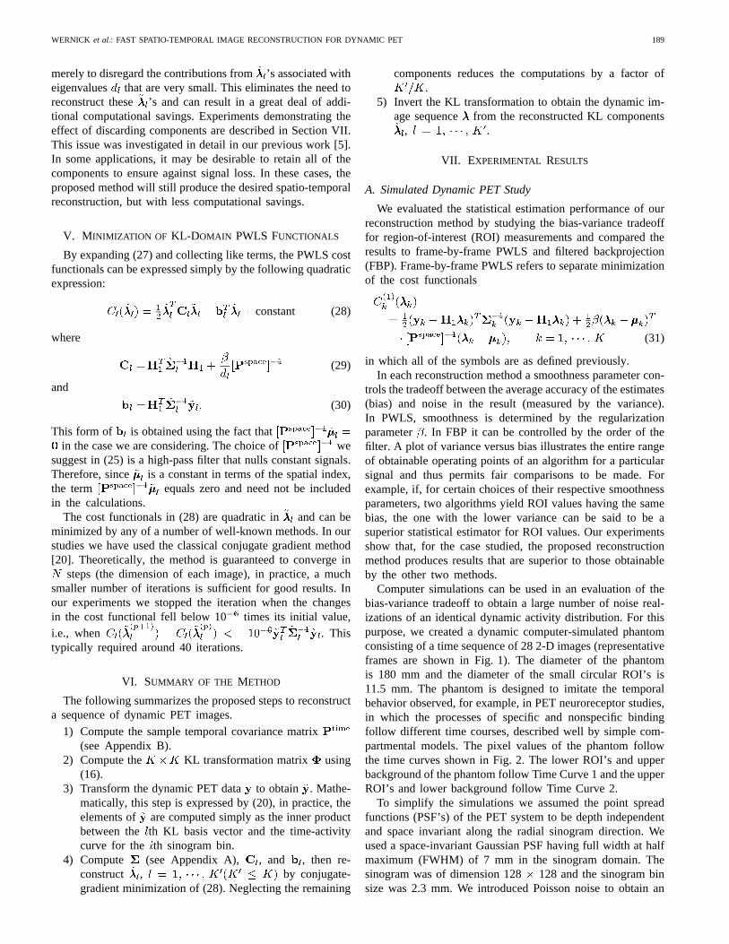
Computer simulations can be used in an evaluation of thebias-variance tradeoff to obtain a large number of noise real-izations of an identical dynamic activity distribution. For thispurpose, we created a dynamic computer-simulated phantomconsisting of a time sequence of 28 2-D images (representativeframes are shown in Fig. 1). The diameter of the phantomis 180 mm and the diameter of the small circular ROI’s is11.5 mm. The phantom is designed to imitate the temporalbehavior observed, for example, in PET neuroreceptor studies,in which the processes of specific and nonspecific bindingfollow different time courses, described well by simple com-partmental models. The pixel values of the phantom followthe time curves shown in Fig. 2. The lower ROI’s and upperbackground of the phantom follow Time Curve 1 and the upperROI’s and lower background follow Time Curve 2.

To simplify the simulations we assumed the point spreadfunctions (PSF’s) of the PET system to be depth independentand space invariant along the radial sinogram direction. Weused a space-invariant Gaussian PSF having full width at halfmaximum (FWHM) of 7 mm in the sinogram domain. Thesinogram was of dimension 128 128 and the sinogram binsize was 2.3 mm. We introduced Poisson noise to obtain an


Fig. 1. Representative image frames from dynamic phantom used in com-puter simulations. Pixels follow one of the time-activity curves shown inFig. 2.

Fig. 2. Time-activity curves followed by pixels in simulated dynamic phan-tom.

average of four million counts for the entire dynamic dataset (divided among the 28 images in accordance with thetime behavior). We also created a realization of the Poisson-distributed randoms contribution for each frame which weused to simulate the effect of randoms precorrection. Weassumed the Poisson randoms rate to be constant throughouteach sinogram and used a randoms fraction of 20% of thetotal counts per scan. We then simulated precorrected PETdata using (5), omitting the corrections for detector efficiencyand attenuation.

The proposed reconstruction method (labeled in the figuresas KL-PWLS) begins with computation of the KL basisvectors. A plot of the resulting eigenvalues for one noiserealization is shown in Fig. 3. Note the dominance of thefirst two eigenvalues. The importance of the first two KLcomponents of the data is reinforced by visual inspection(see Fig. 4). Based on Fig. 3 it appears that beyond ,the KL components of the data are dominated by noise. Inthis study, significance of the components was not assessedrigorously. Fortunately, the number of components to retain isnot critical because the algorithm relies on the discarding ofcomponents only to reduce the computations.

For comparison, we reconstructed each image frame in-dependently by PWLS and by FBP with a Hamming filterwithout any KL transformation. This represents the moreconventional frame-by-frame approach to reconstructing animage sequence in which existing reconstruction methods areapplied separately to each frame.

In implementing frame-by-frame PWLS we used the samespatial regularization operator used in the proposed KL-PWLSmethod. A nonnegativity constraint was not included in eitherimplementation. We did not consider methods for choosing the

Fig. 3. Spectrum of Karhunen–Loève eigenvaluesdl. Note that the first twoare significantly larger than the rest.

Fig. 4. Karhunen–Loève-transformed data~yl for values ofl indicated above.The first two components appear to contain the bulk of the signal information.Components~yl; l = 5; � � � ; 27 (not shown) look very much like~y28.

regularization parameter in either algorithm, but rather studiedthe results obtained by a broad range of parameter values.

The ROI’s in our experiment are the small circular regionsin the phantom. We studied the algorithms’ performance forthe lower ROI’s (Time Curve 1) and upper ROI’s (TimeCurve 2) separately. Plots of the variance versus bias ofestimates of the average activity in the ROI’s (as measuredfrom the reconstructed images) are shown in Fig. 5. The biasand variance are expressed in terms of percentages as follows:

Bias (%) (32)

Variance (%) (33)

where denotes the true activity in one of the sets of ROI’sintegrated over scan interval, is an estimate of made byaveraging over the pixels within the ROI’s in the reconstructedimage, and the overbar denotes a sample mean over 100 noiserealizations.

Results for representative frames are shown in Fig. 5. Notethat for any specified bias level, the proposed KL-PWLS meth-ods can achieve lower variance than either FBP or frame-by-frame PWLS. In this sense, the results obtained by KL-PWLSreconstruction can be said to be superior. It is interesting tonote also that the KL-PWLS method worked best when onlythree KL components were retained, i.e., when . Weattribute this to the excellent noise reduction obtained whenhigh-order KL components are discarded, an effect that wasalso observed in a previous study [5].

We noticed a curious shape to the KL-PWLS bias-variancecurves for the early time frames. In the curve for Frame 1,Time Curve 1, the bias-variance curve extends to near 30%bias, then folds back. We have observed similar curves in


Fig. 5. Variance versus bias of ROI activity in reconstructed images, showing tradeoff between accuracy and noise for various reconstruction algorithms:FBP; frame-by-frame PWLS; and proposed KL-domain method (KL-PWLS), shown with 3, 14, and 28 KL components retained. The graphs in the leftcolumn are for regions of the phantom following Time Curve 1 and the right-column results are for Time Curve 2. Note that the KL-PWLS methods aresuperior to FBP and PWLS, and that the best results overall are obtained by retaining only three components.

previous work by others, e.g., [17], but we are uncertain of thecause. We suspect it may result from premature stopping of theiterative optimization (iterating to completion is impractical).Fortunately, this behavior does not present a problem inpractice because the useful portion of the curve extends overseveral orders of magnitude for the regularization parameter

. The appropriate choice of depends on the imagingapplication: visual appearance usually is best at higher valuesof , However, quantitative measurements are more accurateat lower values for .

A global assessment of performance is given in Fig. 6 whichconsists of plots of the mean absolute bias and mean variancefor the entire image sequence, defined by

Mean Absolute Bias (%) (34)

Mean Variance (%) (35)


Fig. 6. Plots of mean variance versus mean absolute bias. These quantities (defined in the text) summarize the overall performance of the reconstructionalgorithms for the entire image sequence. Note that the KL-PWLS algorithms produce superior results: the best results overall are obtained when onlythree components are retained.

Fig. 7. Examples from reconstructed image sequences having high (approx-imately 25%) mean absolute bias. The best results appear to be obtained bythe proposed KL-PWLS method when only three components are retained.

These plots summarize the statistical properties of the wholeimage sequence. Again, the KL-PWLS methods provideduniformly superior results, and the best results were obtainedwhen the number of retained components is three.

Examples of 128 128 images reconstructed by the meth-ods tested are shown in Figs. 7 and 8. To compare the resultsfairly, images obtained by the different methods are shown atcomparable bias levels. In Fig. 7 the smoothing parameterin PWLS and KL-PWLS and the filter order in FBP werechosen to obtain a bias level of approximately 25%. At acomparable bias level, the FBP and frame-by-frame PWLS

Fig. 8. Examples from reconstructed image sequences with smoothing pa-rameter chosen to produce low (approximately 5%) mean bias. Images areshown at comparable bias levels to fairly compare the results. Filteredbackprojection images are not shown because 5% mean absolute bias was notachievable by this method. Again, KL-PWLS with three retained componentsproduces the best results.

images are visibly noisier than the images obtained by KL-PWLS. Reconstructed images with a bias of about 5% areshown in Fig. 8. Without sinogram restoration FBP cannotachieve low bias, therefore, no FBP images are shown inFig. 8. At both bias levels the images obtained with only threeretained components appear to be best.

The KL-PWLS method produces better results than frame-by-frame PWLS or FBP and can do so with very reasonablecomputation time. Table I shows theoretical formulae forthe relative computation times (normalized to that of FBP)required by the reconstruction methods considered. These wereobtained by counting the numbers of multiply-and-accumulate(MAC) operations. The reason for the long computation timeof the exact spatio-temporal PWLS method is the temporalregularization. Table II shows empirical relative computationtimes for the particular experiments reported in this paper.With three retained components, KL-PWLS required only8.4 times the computation time of FBP to reconstruct the


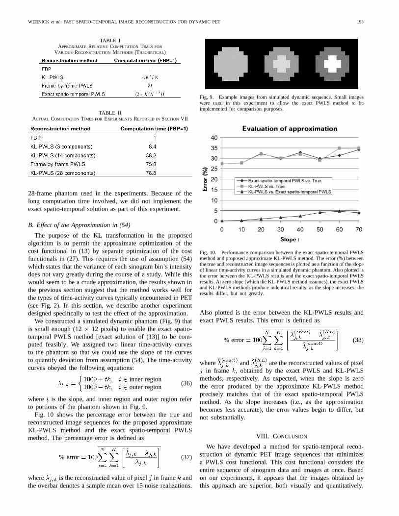
TABLE IAPPROXIMATE RELATIVE COMPUTATION TIMES FOR

VARIOUS RECONSTRUCTIONMETHODS (THEORETICAL)

TABLE IIACTUAL COMPUTATION TIMES FOR EXPERIMENTS REPORTED IN SECTION VII

28-frame phantom used in the experiments. Because of thelong computation time involved, we did not implement theexact spatio-temporal solution as part of this experiment.

B. Effect of the Approximation in (54)

The purpose of the KL transformation in the proposedalgorithm is to permit the approximate optimization of thecost functional in (13) by separate optimization of the costfunctionals in (27). This requires the use of assumption (54)which states that the variance of each sinogram bin’s intensitydoes not vary greatly during the course of a study. While thiswould seem to be a crude approximation, the results shown inthe previous section suggest that the method works well forthe types of time-activity curves typically encountered in PET(see Fig. 2). In this section, we describe another experimentdesigned specifically to test the effect of the approximation.

We constructed a simulated dynamic phantom (Fig. 9) thatis small enough (12 12 pixels) to enable the exact spatio-temporal PWLS method [exact solution of (13)] to be com-puted feasibly. We assigned two linear time-activity curvesto the phantom so that we could use the slope of the curvesto quantify deviation from assumption (54). The time-activitycurves obeyed the following equations:

inner regionouter region

(36)

where is the slope, and inner region and outer region referto portions of the phantom shown in Fig. 9.

Fig. 10 shows the percentage error between the true andreconstructed image sequences for the proposed approximateKL-PWLS method and the exact spatio-temporal PWLSmethod. The percentage error is defined as

% error (37)

where is the reconstructed value of pixelin frame andthe overbar denotes a sample mean over 15 noise realizations.

Fig. 9. Example images from simulated dynamic sequence. Small imageswere used in this experiment to allow the exact PWLS method to beimplemented for comparison purposes.

Fig. 10. Performance comparison between the exact spatio-temporal PWLSmethod and proposed approximate KL-PWLS method. The error (%) betweenthe true and reconstructed image sequences is plotted as a function of the slopeof linear time-activity curves in a simulated dynamic phantom. Also plotted isthe error between the KL-PWLS results and the exact spatio-temporal PWLSresults. At zero slope (which the KL-PWLS method assumes), the exact PWLSand KL-PWLS methods produce indentical results: as the slope increases, theresults differ, but not greatly.

Also plotted is the error between the KL-PWLS results andexact PWLS results. This error is defined as

% error (38)

where and are the reconstructed values of pixelin frame , obtained by the exact PWLS and KL-PWLS

methods, respectively. As expected, when the slope is zerothe error produced by the approximate KL-PWLS methodprecisely matches that of the exact spatio-temporal PWLSmethod. As the slope increases (i.e., as the approximationbecomes less accurate), the error values begin to differ, butnot substantially.

VIII. C ONCLUSION

We have developed a method for spatio-temporal recon-struction of dynamic PET image sequences that minimizesa PWLS cost functional. This cost functional considers theentire sequence of sinogram data and images at once. Basedon our experiments, it appears that the images obtained bythis approach are superior, both visually and quantitatively,


to those produced by conventional frame-by-frame image-sequence reconstruction. A straightforward optimization of thePWLS cost functional involves a lengthy calculation, but,by using the proposed method, we obtained results in aslittle as 8.4 times the computational cost of ordinary filteredbackprojection.

The proposed method has several potential limitations whichwe plan to consider in future work: 1) a nonnegativity con-straint cannot be imposed directly in the KL domain becauseKL coefficients may be negative; 2) a MAP cost functionalwith a precise description of the statistics of precorrected PETdata may be superior to the PWLS cost functional we used inthis paper, especially when the number of counts is very low;3) we have not yet conducted a thorough investigation of theeffect that patient motion might have on the behavior of thealgorithm; and 4) we have not yet implemented a method fordetermining the minimum number of KL components requiredfor good reconstruction.

APPENDIX AESTIMATION OF

As described in Section III

(39)

where

(40)

In principle, is unobservable. In practice, isunrecorded by PET systems that precorrect the data. How-ever, satisfactory estimates of and can be easilyobtained. can be approximated as a smoothed versionof the data obtained using a linear filter. In our experimentswe use a filter having a five-pixel kernel that is cross-shaped,including the center pixel, and extending one pixel forwardand back in time, and one in either direction along the radialsinogram coordinate. The randoms contribution can beestimated as the total delayed-window counts divided by thenumber of sinogram elements.

APPENDIX BESTIMATION OF

To approximate we use a sample covariance matrixobtained from filtered-backprojection reconstructions of thedynamic images (computed using a ramp filter). Letdenote the value of pixel in a filtered-backprojection recon-struction of scan and let represent its sample mean overall pixels, i.e.,

(41)

Then element of can be approximated as

APPENDIX CDERIVATION OF THE PWLS FUNCTIONAL IN THE KL DOMAIN

Inversion of (20) and (21) yields

(42)

and

(43)

Similarly, the mean of can be written as

(44)

Note that and are orthogonal matrices soand . Substituting (23) and (42)–(44) into thePWLS cost functional (13) we obtain

(45)

In a manner similar to that used to derive (19), one can showthat

(46)

Using (46), distributing the transpose operations, and factoringout the transformation matrices we obtain

(47)

Using (17) we rewrite the term in curly braces as follows:

(48)

where is the diagonal matrix ofKL eigenvalues defined by (16). It is easy to show that

(49)

where is the covariance matrix of the data in the space-KLdomain. Using (48) and (49), (47) becomes

(50)

The inverse covariance matrix is of the form

......

.. ....

(51)

in which the blocks are given by

(52)


where

(53)

is the variance matrix of the time-activity curve for sinogrambin and is the th KL basis vector.

If the dynamic PET data do not vary to greatly in time,then the variances are nearly equal andcan be approximated by a constant. In this case, canbe approximated as

(54)

While this would seem to be a rough approximation, the resultsshown in Section VII suggest that it produces good resultsfor time variation characteristic of dynamic PET. In gatedmyocardial imaging the approximation would be even moreappropriate. There, each image frame is a time average, theimages do not reflect tracer dynamics, and the total observedactivity is roughly conserved from frame to frame. Except nearthe edges of the myocardium, the intensity of most pixels ina gated-image sequence remains relatively constant in time.

Based on assumption (54), since the eigenvectorsareorthogonal, the off-diagonal blocks of are approximatelyzero and becomes

...(55)

which is the diagonal variance matrix of. In the followingequations we drop the repeated index on the diagonal blocks,thus is written as which is the variance matrix of theth KL component of .

Because is block diagonal, is diagonal, and isapproximated as diagonal (50) reduces to

(56)

where

(57)

ACKNOWLEDGMENT

The authors are grateful to J. Mukherjee for many helpfuldiscussions regarding receptor imaging.

REFERENCES

[1] J. A. Fessler, “Penalized weighted least-squares image reconstructionfor positron emission tomography,”IEEE Trans. Med. Imag.,vol. 13,pp. 290–300, June 1994.

[2] D. S. Lalush and B. M. W. Tsui, “Space-time Gibbs priors appliedto gated SPECT myocardial perfusion,” inThree-Dimensional Im-age Reconstruction in Radiology and Nuclear Medicine, ComputationalImaging and Vision,P. Grangeat, J-L, and Amans, Eds. Dordrecht, TheNetherlands: Kluwer, 1996, pp. 209–224.

[3] , “A priori motion models for four-dimensional reconstruction ingated cardiac SPECT,” in1996 Conf. Record Nuclear Science Symp.Medical Imaging Conf.,1997.

[4] , “Block-iterative techniques for fast 4D reconstruction usingapriori motion models in gated cardiac SPECT,”Phys. Med. Biol.,vol.43, pp. 875–886, 1998.

[5] C.-M. Kao, J. T. Yap, J. Mukherjee, and M. N. Wernick, “Imagereconstruction for dynamic PET based on low-order approximation andrestoration of the sinogram,”IEEE Trans. Med. Imag.,vol. 16, pp.738–749, Dec. 1997.

[6] M. N. Wernick, G. Wang, C.-M. Kao, J. T. Yap, J. Mukherjee, M.Cooper, and C.-T. Chen, “An image reconstruction method for dynamicPET,” in 1995 Conf. Record Nuclear Science Symp. Medical ImagingConf., 1996.

[7] V. M. Narayanan, M. A. King, E. Soares, C. Byrne, H. Pretorius, andM. N. Wernick, “Application of the Karhunen–Loève transform to 4Dreconstruction of gated cardiac SPECT images,” in1997 Conf. RecordNuclear Science Symp. Medical Imaging Conf.,1998.

[8] N. P. Galatsanos and R. T. Chin, “Digital restoration of multichannelimages,” IEEE Trans. Acoust., Speech, Signal Processing,vol. 37, pp.415–421, Mar. 1989.

[9] N. P. Galatsanos, A. K. Katsaggelos, R. T. Chin, and A. D. Hillery,“Least squares restoration of multichannel images,”IEEE Trans. SignalProcessing,vol. 39, pp. 2222–2236, Oct. 1991.

[10] N. P. Galatsanos and R. T. Chin, “Restoration of color images bymultichannel Kalman filtering,”IEEE Trans. Signal Processing,vol. 39,pp. 2237–2252, Oct. 1991.

[11] B. R. Hunt and O. Kubler, “Karhunen–Loeve multispectral imagerestoration—Part 1: Theory,”IEEE Trans. Acoust., Speech, Signal Pro-cessing,vol. ASSP-32, pp. 592–599, June 1984.

[12] P. J. Ready and P. A. Wintz, “Information extraction, SNR improvement,and data compression in multispectral imagery,”IEEE Trans. Commun.,vol. 21, pp. 1123–1130, June 1973.

[13] J. B. Lee, S. Woodyatt, and M. Berman, “Enhancement of high spectralresolution remote-sensing data by a noise-adjusted principal componentstransform,”IEEE Trans. Geosci. Remote Sensing,vol. 28, pp. 295–304,May 1990.

[14] D. C. Barber, “The use of principal components in the quantitativeanalysis of gamma camera dynamic studies,”Phys. Med. Biol.,vol. 25,pp. 283–292, 1980.

[15] J. T. Yap, J. D. Treffert, C.-T. Chen, and M. D. Cooper, “Imageprocessing of dynamic images with principal component analysis,”Radiology,vol. 185(p), p. 177, 1992.

[16] S. M. Kay, Fundamentals of Statistical Signal Processing: EstimationTheory. Englewood Cliffs, NJ: Prentice-Hall, 1993.

[17] E. U. Mumcuoglu, R. M. Leahy, Z. Zhou, and S. R. Cherry, “A phantomstudy of the quantitative behavior of Bayesian PET reconstructionmethods,” in1996 Conf. Record Nuclear Science Symp. Medical ImagingConf., 1997.

[18] A. K. Jain, Fundamentals of Digital Image Processing.Upper SaddleRiver, NJ: Prentice-Hall, 1989.

[19] A. A. Green, M. Berman, P. Switzer, and M. D. Craig, “A transfor-mation for ordering multispectral data in terms of image quality withimplications for removing noise,”IEEE Trans. Geosci. Remote Sensing,vol. 26, pp. 65–74, Jan. 1988.

[20] E. Z. P. Chong and S. H. Zak,An Introduction to Optimization. NewYork: Wiley, 1996.

Documents

Fast spatio-temporal image reconstruction for dynamic PET