Embed Size (px)
Citation preview

General rights Copyright and moral rights for the publications made accessible in the public portal are retained by the authors and/or other copyright owners and it is a condition of accessing publications that users recognise and abide by the legal requirements associated with these rights.
Users may download and print one copy of any publication from the public portal for the purpose of private study or research.
You may not further distribute the material or use it for any profit-making activity or commercial gain
You may freely distribute the URL identifying the publication in the public portal If you believe that this document breaches copyright please contact us providing details, and we will remove access to the work immediately and investigate your claim.
Downloaded from orbit.dtu.dk on: Jan 17, 2020
Fast Generation of Container Vessel Stowage Plansusing mixed integer programming for optimal master planning and constraint based localsearch for slot planningPacino, Dario; Jensen, Rune Møller
Publication date:2012
Link back to DTU Orbit
Citation (APA):Pacino, D., & Jensen, R. M. (2012). Fast Generation of Container Vessel Stowage Plans: using mixed integerprogramming for optimal master planning and constraint based local search for slot planning. IT University ofCopenhagen.

IT University of Copenhagen
Ph.D. Thesis
Fast Generation of Container VesselStowage Plans
using mixed integer programming for optimal master planning and
constraint based local search for slot planning
Author:Dario Pacino
Supervisor:Assoc.Prof. Rune Møller Jensen
October 5, 2012
Preface
During my undergraduate studies, I have always been focused on becoming a goodsoftware designer and programmer. During my master studies at the IT-Universityof Copenhagen I met Rune Møller Jensen who proposed I do a project within theshipping domain. Without even realizing it I was thrown into the abyss of research,which changed my career plans drastically. I wanted to be a researcher. I was verythankful when the Dansk Maritim Fond granted me a full Ph.D. scholarship at theIT-University of Copenhagen with Rune Møller Jensen as my supervisor.
The road to the successful conclusion of this Ph.D. project was not smooth. Verylittle was known about the details of container stowage. There is no book telling thewhole story. In some way I hope this Ph.D. thesis can cover this knowledge gap forfuture researchers. The years of industrial collaboration and the hard work of everyoneinvolved in this project has contributed to its success.
During my Ph.D. studies I also have had the pleasure of visiting Professor Pascal VanHentenryck at Brown University for a period of 5 months. During the visit I worked ondecomposition techniques for scheduling problems. The results of this project are pub-lished in peer-reviewed venues. I have also had the pleasure to work with my colleaguesfrom the Decision Optimization Lab, Alberto Delgado and Kevin Tierney, and withYuri Malitsky on a machine assignment problem for a competition organized by EURO(European Conference on Operations Research), for which we have qualified. Thesecollaborations have undoubtedly contributed to broadening my research prospectivesand finally to the completion of my Ph.D. study.
2

Abstract
Containerization has changed the way the world perceives shipping. It isnow possible to establish complex international supply chains that haveminimized shipping costs. Over the past two decades, the demand for costefficient containerized transportation has seen a continuous increase. In or-der to answer to this demand, shipping companies have deployed biggercontainer vessels, that nowadays can transport up to 18,000 containers andare wider than the extended Panama Canal. Like busses, container ves-sels sail from port to port through a fixed route loading and dischargingthousands of containers. Before the vessel arrives at a port, it is the jobof a stowage coordinator to devise a stowage plan. A stowage plan is adocument describing where each container should be loaded in the vesselonce terminal operations commence. When creating stowage plans, stowagecoordinators must make sure that the vessel is stable and seaworthy, and atthe same time arrange the cargo such that the time at port is minimized.Moreover, stowage coordinators only have a limited amount of time to pro-duce the plan. This thesis addresses the question of whether it is possibleto automatically generate stowage plans to be used by stowage coordina-tors, and it advocates that the quality of the stowage plans and the timein which they can be generated is of the outmost importance for practicalusage. We introduce a detailed description of a representative problem ofthe computational complexity of stowage planning that has enough detailto allow professionals from the industry to evaluate its solutions. A 2-phasehierarchical decomposition of the problem is presented. In the first phase,the problem of distributing containers to sections of the vessel is solved,and it is here that the seaworthiness of the solution is evaluated. In thesecond phase, the assignment of containers is refined to specific positionswithin the ship and lower level constraints are handled. The approach hasbeen implemented with a combination of operations research and artificialintelligence methods, and has produced promising results on real test in-stances provided by a major liner shipping company. Improvements to themodeling of vessel stability and an analysis of its accuracy together with ananalysis of the computational complexity of the container stowage problemare also included in the thesis, resulting in an overall in-depth analysis ofthe problem.
3
Acknowledgments
Obtaining a Ph.D. is hardly a task one does alone, and in this regard I would like toexpress my thanks to the people that have been helpful and supportive through out mystudies.
First of all, I must thank my wife Heidi and my children Leo, Anna and Luca. Thesupport and joy that a family can give, is, in my opinion, invaluable to endure theperiods of frustration that can afflict us during research. They have been running alongside with me in the marathon that writing this thesis has been.
I was very lucky to have Rune Møller Jensen as supervisor, and I would like to thankhim for all his constructive comments and for always being excited and supportive ofmy research. He not only supported my research, but also made quite an effort to helpme with my future academic career. I regard him as my mentor and most of all as afriend.
Thanks must also go to Alberto Delgado, Kevin Tierney and all of the SoftwareDevelopment Group at the IT-University of Copenhagen for all their comments, ad-vises and for taking me out for beers. I would also like to thank the IT-University ofCopenhagen and all the administrative staff for their support and friendliness.
A special thanks goes to Carsten Melchiors and Den Danske Maritime Fond forgrating fonds for the entire Ph.D. study. Without them this thesis would not exist.Ange Optimization and Mærsk Line, have also been invaluable to this research and Ithank them for providing all the needed data and for answering countless questions. Inparticular I would like to thank Kim Hansen, Nicolas Guilbert, Niels Christensen andTom Bebbington.
During my study I have met a number of very interesting people. One in par-ticular is Professor Pascal Van Hentenryck, whom has been so kind to have me asvisiting researcher at Brown University. I would like to thank him, and all of the fellowresearchers, that I have meet in different scientific conference and meeting, for theirquestions, criticism and interest in my research. My thanks must also go to all theanonymous reviewers of my articles and papers for their hard work.
Last, but not least, I would like to thank the members of the thesis assessment com-mittee: Stefan Voß, David Pisinger and Thore Husfeldt for all their valuable commentsand dedication.
4
CONTENTS
Contents
1 Introduction 71.1 Thesis Question . . . . . . . . . . . . . . . . . . . . . . . . . . . . . . . 81.2 Thesis Contributions . . . . . . . . . . . . . . . . . . . . . . . . . . . . 101.3 Publications . . . . . . . . . . . . . . . . . . . . . . . . . . . . . . . . . 101.4 Document Outline . . . . . . . . . . . . . . . . . . . . . . . . . . . . . 11
2 Container Stowage Planning 132.1 Container Terminals . . . . . . . . . . . . . . . . . . . . . . . . . . . . 132.2 Standard Containers . . . . . . . . . . . . . . . . . . . . . . . . . . . . 152.3 Container Vessels . . . . . . . . . . . . . . . . . . . . . . . . . . . . . . 172.4 Vessel Stability and Stress Limits . . . . . . . . . . . . . . . . . . . . . 182.5 Container Stowage . . . . . . . . . . . . . . . . . . . . . . . . . . . . . 222.6 Stowage Plans . . . . . . . . . . . . . . . . . . . . . . . . . . . . . . . . 23
3 Related Work 253.1 Single Model Approaches . . . . . . . . . . . . . . . . . . . . . . . . . . 253.2 Decomposition Models . . . . . . . . . . . . . . . . . . . . . . . . . . . 29
4 Representative Problem and Algorithmic Framework 314.1 A Representative Problem . . . . . . . . . . . . . . . . . . . . . . . . . 31
4.1.1 Container Types . . . . . . . . . . . . . . . . . . . . . . . . . . 314.1.2 Vessel Layout and Routes . . . . . . . . . . . . . . . . . . . . . 324.1.3 Vessel Stability . . . . . . . . . . . . . . . . . . . . . . . . . . . 324.1.4 Container Stowage . . . . . . . . . . . . . . . . . . . . . . . . . 334.1.5 Container Stowage Objectives . . . . . . . . . . . . . . . . . . . 334.1.6 The Proposed Problem . . . . . . . . . . . . . . . . . . . . . . . 34
4.2 The Quad Framework . . . . . . . . . . . . . . . . . . . . . . . . . . . 34
5 Master Planning 375.1 A Model for Master Planning . . . . . . . . . . . . . . . . . . . . . . . 385.2 Complexity of the Master Planning Problem . . . . . . . . . . . . . . . 415.3 Computational Results . . . . . . . . . . . . . . . . . . . . . . . . . . . 425.4 An Improved Stability and Stress Model . . . . . . . . . . . . . . . . . 47
5

CONTENTS
5.4.1 Linearization of stability constraints . . . . . . . . . . . . . . . . 475.4.2 A Revised Model with Ballast Tanks . . . . . . . . . . . . . . . 505.4.3 Analysis of Model Accuracy . . . . . . . . . . . . . . . . . . . . 53
6 Slot Planning 596.1 The Slot Planning Problem . . . . . . . . . . . . . . . . . . . . . . . . 596.2 Constraint-Based Local Search (CBLS) . . . . . . . . . . . . . . . . . . 626.3 A CBLS for Slot Planning . . . . . . . . . . . . . . . . . . . . . . . . . 63
6.3.1 Constraint Violations . . . . . . . . . . . . . . . . . . . . . . . . 646.3.2 Objective Violations . . . . . . . . . . . . . . . . . . . . . . . . 666.3.3 Incremental evaluation . . . . . . . . . . . . . . . . . . . . . . . 666.3.4 Placement heuristic . . . . . . . . . . . . . . . . . . . . . . . . . 696.3.5 The Search Strategy . . . . . . . . . . . . . . . . . . . . . . . . 70
6.4 Experimental Evaluation . . . . . . . . . . . . . . . . . . . . . . . . . . 736.5 Dealing with Fractional and Infeasible Instances . . . . . . . . . . . . . 75
7 Conclusions 797.1 Outlook and Future Directions . . . . . . . . . . . . . . . . . . . . . . . 80
A Complexity Analysis 83A.1 The k-Shift Problem . . . . . . . . . . . . . . . . . . . . . . . . . . . . 83A.2 UkSP is NP-Complete . . . . . . . . . . . . . . . . . . . . . . . . . . . 84A.3 Complexity of CkSP . . . . . . . . . . . . . . . . . . . . . . . . . . . . 85A.4 The Hatch Overstow Problem . . . . . . . . . . . . . . . . . . . . . . . 85A.5 Remarks . . . . . . . . . . . . . . . . . . . . . . . . . . . . . . . . . . . 87
B Decomposition in Scheduling 89B.1 Constraint Based Decompositions for Scheduling Problems . . . . . . . 89B.2 The Flexible Jobshop Problem . . . . . . . . . . . . . . . . . . . . . . . 90B.3 Prior Work . . . . . . . . . . . . . . . . . . . . . . . . . . . . . . . . . 90B.4 A Constraint-Based Scheduling Model . . . . . . . . . . . . . . . . . . 91B.5 Large Neighborhood Search . . . . . . . . . . . . . . . . . . . . . . . . 91B.6 Adaptive Randomized Decompositions . . . . . . . . . . . . . . . . . . 93
B.6.1 Time Decomposition . . . . . . . . . . . . . . . . . . . . . . . . 93B.6.2 Machine Decomposition . . . . . . . . . . . . . . . . . . . . . . 95B.6.3 Solution Merging . . . . . . . . . . . . . . . . . . . . . . . . . . 96
B.7 Experimental Evaluation . . . . . . . . . . . . . . . . . . . . . . . . . . 96B.8 Concluding Remarks . . . . . . . . . . . . . . . . . . . . . . . . . . . . 100
C Completeness of the CBLS neighborhood 101
6

Chapter 1. Introduction
Chapter 1
Introduction
The world economy has always been heavily dependent on the ability of transportinggoods. In the years up to the 1950’s companies were operating mainly in local marketswhere the competitive advantage depended on how close to the customers the productswere manufactured. After 1955, with the introduction of containerized shipping, allthis changed. Containers made it possible to transport products across the oceanswith reduced cost and complexity. The world’s economy changed to a global economy,where Asian manufacturing companies could sell their products to the rest of the worldat lower costs than others, and where supply chains grew larger and more international(Levinson, 2006).
Liner shipping companies faced this increasing demand by building larger ships,that nowadays can carry up to 18,000 containers. We also saw the creation of special-ized harbors that only handle container shipping, easing intermodal transportation andsupporting this new global economy.
Employing larger ships, however, is not enough for shipping companies to respondto the demand for cheap transportation. The load of containers on a vessel must beoptimized so costs can be reduced. The distribution of containers defines how thevessel sits in the water, and thus influences its bunker consumption. Moreover, loadand discharge operations at container terminals are costly, ergo reducing the numberof moves and the total time at port is essential to achieving cost reductions.
It is the job of stowage coordinators to ensure that the containers are correctlystowed in the vessel in a cost efficient way. Stowage coordinators manually producea stowage plan 1. Stowage plans define the exact position of each container withina vessel and are used by container terminals during load and discharge operations.Stowage planning is a central component in the liner shipping industry and can beused in different contexts. For example, it can be used by string managers for thedesign of cargo flows in a shipping network, where stowage plans define the possiblecontainer intakes of the vessels given a specific mixture of cargo. In container terminals,sequencing operations (the decision of which container to be taken from the yard at
1Stowage plans, container ship stowage plans and container stowage plans will be used interchange-ably in this thesis.
7
Chapter 1. Introduction
which point in time), are strongly affected by each vessel stowage plan. Integrationof stowage planning into terminal sequencing would improve terminal operations evenmore.
Cost-efficient stowage plans, however, are hard to produce in practice. First, theyare made under pressure of time just hours before the vessel calls the port. Second,large deep-sea vessels often require thousands of container moves in a port. Third,complex interactions between low-level stacking rules and high-level stress limits andstability requirements make it difficult to minimize time at port. Finally, robust plansrequire stowage coordinators to evaluate the consequences of decisions in down-streamports. Information about containers in further ports is, however, scarce and based onforecasting so several scenarios might need to be generated before a final plan can bereleased.
From a research point of view, it is also hard to access information about stowageplanning. Detailed information about vessel designs is necessary in order to producecorrect stability and stress calculations. This data is considered confidential and thusvery hard to access without close collaboration with the industry. Expert knowledgeabout stowage planning itself is also very important, but no book written about stowageplanning exists. Knowledge must be extracted from various guides, companies’ internaldocumentations and the experience of senior staff.
These barriers did not stop academics from developing an interest in this problem,and the past decades have seen a growing number of works published in the litera-ture. Previous work on the stowage planning problem has been innovative on solutionapproaches, but has been challenged by the inaccessibility of the problem. This haslead to limited representative power of the developed models and a lack of benchmarkproblems.
1.1 Thesis Question
This thesis is based on a long term collaboration with a large liner shipping company,and thus has the opportunity to breach the knowledge and data barrier and deliverhighly representative research findings. This thesis aims at answering a question that,according to the results shown in the literature, has yet to receive a positive answer:
“Can container ship stowage plans with high enough quality for practicalusage be computed on standard equipment within the time required by thework processes of stowage coordinators?”
In order to fully understand this question, it is important to clarify some of the keyaspects the question is built upon. The first of those aspects is “high enough quality.”Like many other industrial problems, stowage planning is riddled with details, specialcases and solution preferences. This thesis does not aim at generating stowage planningalgorithms that can substitute human stowage coordinators. We believe that both theresearch field and the current technology is not ready for such a challenge. This thesis
8
Chapter 1. Introduction
aims at producing stowage plans that can be used by human stowage coordinators asguidance in the decision making process of generating a final stowage plan. More specif-ically, automated stowage planning should model all key aspects of stowage planningsuch that an automatically generated stowage plan can be used as a reference solutionthat can easily be modified into a final plan.
The second important aspect of the thesis’ question is “computed on standard equip-ment.” Shipping companies have teams of stowage coordinators and it would be un-reasonable to believe that each coordinator is equipped with a super computer. Weaim at identifying the possibility of answering the thesis question using hardware thatis affordable, but still has high quality properties. The work presented in this thesis isbased on hardware corresponding to 8-12 AMD Opteron processors on a single machine.
The last, and most restrictive aspect or requirement of the thesis question is “withinthe time required by the work processes of stowage coordinators.” Stowage coordinatorshave a limited number of hours to produce the final stowage plan, however one mustconsider that the stochastic nature of the forecasts used during stowage planning forcescoordinators to consider different scenarios. Should an automated stowage planning tooltake too long to produce plans, it would not be possible for the stowage coordinator toconsider all the necessary scenarios. Moreover, it is often the case that in problems ascomplex as stowage planning, software only solves an abstraction of the problem andthus stowage coordinators must also spend time on final adjustments. In accordancewith our industrial collaborators it was estimated that 10 minutes is the maximumamount of time that a piece of software should take to deliver an answer, if it is to beused during the everyday planning process.
The thesis attempts to answer the thesis question in a two phase research process.Initially we analysed the currently available software packages and documentation tocollect all of the necessary knowledge. As questions arose, the expert knowledge ofstowage coordinators was used to fill-in the gaps. With all the collected informationit was possible, with the agreement of our industrial collaborators, to define a set ofstowage planning aspects that any software package should have in order to be consid-ered representative. With a representative problem at hand, the second phase of theresearch project focuses on the design of efficient algorithms for stowage planning. The10 minutes required by the industry is a relatively short time to solve a complex andlarge scale problem such as stowage planning. The literature has shown that monolithicapproaches tend to fail even on small instances (e.g. Ambrosino and Sciomachen (2003);Giemsch and Jellinghaus (2004); Li et al. (2008)), while multi-phase approaches haveshown promising results, (e.g. Wilson and Roach (1999); Kang and Kim (2002); Am-brosino et al. (2010)). This thesis, inspired by those last two works, presents a 2-phaseapproach to stowage planning that is able to reach phase-wise optimal solutions withinthe required time. An initial phase distributes containers into stowage areas along thevessel while satisfying stability and stress forces and optimizing time at port. A secondphase then assigns specific positions to containers within each of the stowage areas whilesatisfying low-level constraints such as stacking rules and robustness requirements. Thepositive results obtained also motivated an extension of the current model to include
9

Chapter 1. Introduction
more accurate stability and stress calculations.
1.2 Thesis Contributions
The thesis has four major contributions:
1. Accurate modelsThe models presented in this thesis are the most accurate models published inthe literature available. The master planning models include key aspects aboutstress forces and vessel stability that have not yet been presented in the literature.Solution objectives that guide the search toward robust stowage plans are also anovel part of this thesis’ work.
2. Optimal master planningThis thesis presents the first optimal master plans.
3. Fast approachThe models and algorithms presented in this thesis are the fastest among thosetaking into account similar stowage planning aspects.
4. Many instancesThis thesis presents the first results that are based on a large set of industrialbenchmark instances. The instances are generated from stowage problems thathave sailed and thus are highly representative.
It should be noted that only three Ph.D. thesis have been published on the con-tainer stowage problem: Aslidis (1989), Wilson (1997), and Kaisar (1999). The lasthas, however, no related publications. Besides the above contributions, as part of thecollaboration with Professor Pascal Van Hentenryck, a number of contributions havebeen made in the field of constraint based scheduling:
1. First Decoupling Analysis Of Flexible Jobshop SchedulingTo the best of our knowledge this thesis presents the first application of decouplingtechniques to scheduling problems.
2. Improved Best Solutions On Standard BenchmarksThe algorithms implemented in this thesis have brought many new best solutionsto standard flexible jobshop scheduling benchmarks.
1.3 Publications
• Pacino, D. and R. M. Jensen (2012).Constraint-based local search for con-tainer stowage slot planning. In Proceedings of the International MultiCon-ference of Engineers and Computer Scientists, pp. 1467-1472.
10
Chapter 1. Introduction
• Pacino, D., A. Delgado, R. Jensen, and T. Bebbington (2011). Fast generationof near-optimal plans for eco-efficient stowage of large container vessels.Computational Logistics, Volume 6971 of Lecture Notes in Computer Science, pp.286-301.
• Pacino, D. and R. M. Jensen (2010). A 3-phase randomized constraint basedlocal search algorithm for stowing under deck locations of containervessel bays. Technical Report TR-2010-123, IT-University of Copenhagen.
• Pacino, D., A. Delgado, R. Jensen, and T. Bebbington (2012b). Large-scalecontainer vessel stowage planning using mixed integer and constraintprogramming. Under review at Transportation Science.
• Pacino, D., A. Delgado, R. Jensen, and T. Bebbington (2012a). An accuratemodel for seaworthy stowage planning with ballast tank. Under reviewfor the 3rd International Conference on Computational Logistics, (ICCL12).
• Pacino, D., K. Tierney, and R. M. Jensen (2012). NP-hard components ofcontainer vessel stowage planning. To be submitted to OR Letters.
• Pacino, D. and R. M. Jensen (2009). A local search extended placementheuristic for stowing under deck bays of container vessels. ExtendedAbstract in The 4th Int. Workshop on Freight Transportation and Logistics(ODYSSEUS-09).
• Pacino, D., A. Delgado, and R. Jensen (2012). Modeling ballast water incontainer stowage planning. Accepted for presentation at the 25th EuropeanConference on Operational Research (EURO 2012), 8-11 July 2012, Vilnius (LT).
1.4 Document Outline
Chapter 2 Container Stowage Planning. This chapter introduces the reader tothe domain of liner shipping, providing the necessary knowledge and terminologyfor a full understanding of the container stowage problem. This chapter is basedon both the knowledge accumulated during our collaboration with the industryand the book on naval architecture by Tupper (2009).
Chapter 3 Related Work. This chapter gives, to the best of our knowledge, a com-plete review of all the academic work on the container stowage problem.
Chapter 4 Representative Problem and Algorithmic Framework This chapterpresents the representative problem that is solved as part of the work in this the-sis. Remarks about the abstractions and assumptions are also presented. In thischapter we also introduce the 2-phase solution framework, called Quad, used tosolve the container stowage problem.
11

Chapter 1. Introduction
Chapter 5 Master Planning. This chapter describes the first phase of the Quadapproach to container stowage planning. In particular it introduces a MixedInteger Programming (MIP) model that can solve the master planning phaseand provides evidence of its efficiency. Later in the chapter, a refinement of themodel that focuses on achieving high precision for the stability calculations, isalso presented.
This chapter is based on the papers of Pacino et al. (2011), Pacino et al. (2012b),and Pacino et al. (2012a). Note that the defendant has made significant contri-butions to these papers and the implementation methods.
Chapter 6 Slot Planning. This chapter presents a detailed description of the CBLSalgorithm used to solve the slot planning problem in the second phase of the Quadframework. The neighborhood, heuristics, and incremental calculations used inthe algorithm are described in detail together with the experimental results thatshow evidence of the solution method’s efficiency.
This chapter is based on papers by Pacino and Jensen (2009), Pacino and Jensen(2010) and Pacino and Jensen (2012). The defendant is responsible for the im-plementation of the methods and is the main contributor to the papers.
Chapter 7 Conclusions. This chapter ends the thesis with the presentation of con-cluding remarks and giving an outlook of future work and possible research di-rections.
Appendix A Complexity Analysis This appendix introduces previous work on thecomputational complexity of the container stowage problem, and presents newresults. In particular we prove that the Hatch Overstow Problem is NP-Complete.
This chapter is the extended and revised version of the paper by Pacino et al.(2012), in which the defendant made significant contributions.
Appendix B Decomposition in Scheduling. This appendix describes the work donein collaboration with Professor Pascal Van Hentenryck. It presents the applica-tion of decomposition methods to the flexible jobshop problem. Particular focusis given to the Adaptive Randomized Decomposition framework that, for the firsttime, is being applied to scheduling problems.
This chapter is based on the paper by Pacino and Hentenryck (2011). The de-fendant is responsible for the implementation of the methods and is the maincontributor to the papers.
12

Chapter 2. Container Stowage Planning
Chapter 2
Container Stowage Planning
Seaborne shipping is nowadays the most used shipping mode. In general there are threemain seaborne shipping modes: industrial, tramp and liner. In industrial shipping itis the owner of the cargo that owns the fleet and focuses on the minimization of cargotransports costs. Tramp ships are operated like taxis, transporting available cargo todestinations. It is often the case that such shipping companies have contractual com-mitments with cargo companies. In liner shipping, vessels are assigned a route (orstring) and follow a specific schedule. Liner shipping is the preferred mode for con-tainerized transportation and it is the assumed transportation mode in the remainderof this thesis.
Containerization is the transportation of cargo into metallic boxes called containers.Containers are transported by container vessels, which are ships specially designed forthe transportation of containers. Such vessels can carry thousands of containers witha small crew. In general we will talk about 20’ and 40’ long containers and refer tothe space occupied by a 20’ container as a Twenty-foot Equivalent Unit (TEU). Thismeans that a 40’ container is equivalent to two TEUs.
2.1 Container Terminals1
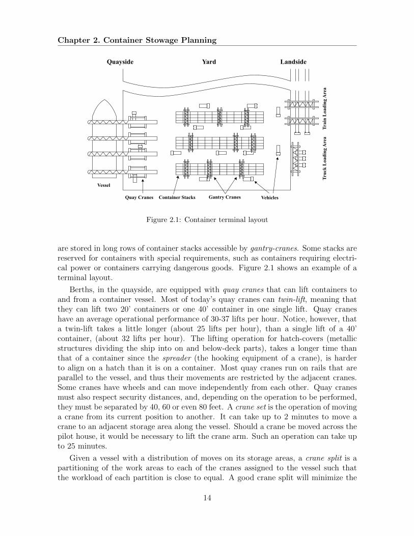
Container terminals are specialized harbors for the handling of containers. When acontainer vessel arrives at the terminal, it is assigned a berth where load and dischargeoperations will be performed. Terminals are divided into three main areas, the quayside,where the berths and the vessels are, the yard, which is a temporary storage area forcontainers, and the landside where truck and train operations are performed. Importcontainers are unloaded from the vessels and transported either to the yard, especiallyin case of transshipments, or directly to the landside for inland transportation. Theopposite cargo flow applies for export containers. Container movements between thequayside, the yard and the landside can be performed by trucks with trailers, multitrail-ers, Automated Guided Vehicles (AGVs) or straddle carriers. Containers in the yard
1Inspired by Steenken et al. (2004)
13
Chapter 2. Container Stowage Planning
Quayside Landside
Vessel
Quay Cranes Gantry Cranes Vehicles
Tra
in L
oad
ing A
rea
Tru
ck L
oad
ing A
rea
Container Stacks
Yard
Figure 2.1: Container terminal layout
are stored in long rows of container stacks accessible by gantry-cranes. Some stacks arereserved for containers with special requirements, such as containers requiring electri-cal power or containers carrying dangerous goods. Figure 2.1 shows an example of aterminal layout.
Berths, in the quayside, are equipped with quay cranes that can lift containers toand from a container vessel. Most of today’s quay cranes can twin-lift, meaning thatthey can lift two 20’ containers or one 40’ container in one single lift. Quay craneshave an average operational performance of 30-37 lifts per hour. Notice, however, thata twin-lift takes a little longer (about 25 lifts per hour), than a single lift of a 40’container, (about 32 lifts per hour). The lifting operation for hatch-covers (metallicstructures dividing the ship into on and below-deck parts), takes a longer time thanthat of a container since the spreader (the hooking equipment of a crane), is harderto align on a hatch than it is on a container. Most quay cranes run on rails that areparallel to the vessel, and thus their movements are restricted by the adjacent cranes.Some cranes have wheels and can move independently from each other. Quay cranesmust also respect security distances, and, depending on the operation to be performed,they must be separated by 40, 60 or even 80 feet. A crane set is the operation of movinga crane from its current position to another. It can take up to 2 minutes to move acrane to an adjacent storage area along the vessel. Should a crane be moved across thepilot house, it would be necessary to lift the crane arm. Such an operation can take upto 25 minutes.
Given a vessel with a distribution of moves on its storage areas, a crane split is apartitioning of the work areas to each of the cranes assigned to the vessel such thatthe workload of each partition is close to equal. A good crane split will minimize the
14

Chapter 2. Container Stowage Planning
56 3656 12 45 27 4 33 3 10 31 24 15 845
113 123 10465
Figure 2.2: A crane split with 4 cranes
makespan of the load and discharge operations and thus minimize the time at port. Anexample crane split of 4 cranes for a vessel with 15 storage areas is shown in Figure 2.2.
It is important to discuss crane productivity since a vessel not only has to pay a feefor each move (load or discharge operation), but also for the team operating the cranesand the cost of the vehicles feeding the cranes. The total move cost is thus linear in thenumber of cranes utilized. The move cost, however, is often outweighed by the need forreducing the time at port.
2.2 Standard Containers
Containers are metallic boxes designed to withstand significant outer forces. Theyare particularly robust to high vertical compression, which allows the creation of highstacks. All containers are fitted with corner castings designed to support the container’sweight, and to which security fittings can be attached. ISO standard containers areusually 20’, 40’ or 45’ long. In the US trade it is also possible to find 48’ or 53’containers that are non-standard in liner shipping. ISO containers are 8’ wide and 8.6’tall with the exception of high-cube containers which are 1 foot taller. Figure 2.3 showsan illustration of a 20’ container, a 40’ container, and a 45’ high-cube container. Longercontainers, such as the 45’ containers are equipped with two extra sets of castings ata 40’ distance. The extra castings allow longer containers to be stacked on top of40’ containers. No castings, however, exist at the 20’ position, which means that 20’containers cannot be stacked on top of longer containers. Note, however, that on-deckit is often not allowed to stack 40’ containers on top of longer ones, since it becomesdifficult to attach security fittings.
Aside from the standard and high-cube containers discussed above, there are anumber of specialized containers for different kinds of cargo. Fruits and vegetables, forexample, must be transported in refrigerated containers. There are two kinds of refrig-erated containers, reefer, which have an integrated refrigeration unit and thus must beconnected to power supplies, and insulated containers, which have more internal capac-ity than a reefer container since they do not have an integrated refrigeration unit andthus must be connected to the vessel’s internal cooling plant when on board. Venti-lated containers have small openings allowing air circulation and do not require externalpower. Fluids, foodstuffs, chemicals and hazardous cargo are often transported in tankcontainers. Some of the cargo in tank containers might need to be kept heated andtherefore those containers might also need to be plugged into power supplies. Food-
15

Chapter 2. Container Stowage Planning
Corner Casting
High Cube Container
20.0'
40.0'45.0'
8.0'
8.0'
8.0'
8.6'9.6'
Figure 2.3: Dimensions of the most common ISO standard containers
stuffs, cereals and spices are also often transported in bulk containers where cargo canbe loaded through three hatches on the top. Cargo with non-standard dimensions, suchas overweight or tall cargo, is transported in Out-Of-Gauge (OOG) containers. Withinthis category we find hard-top containers with a removable roof, open-top containerswithout a roof, flatrack containers with only two end-walls that can be collapsed, andplatforms for heavy and oversized cargo.
In order to better fit Euro-pallets, pallet-wide containers use the 2 inch (ca. 5 cm),space between container stacks to enlarge their capacity. Based on the stacking rulesthat those containers follow, they are divided into three categories: PW0 which do notneed any special stacking rules, PW3 which can be stacked side by side but require astandard container every two PW3s, and PW6 which cannot be stacked side by side.Figure 2.4 shows two valid stacking configurations including a PW6 container. Noticehow the stacking rules involve more containers as palletwides are mixed with high-cubes.
PW6PW6
HQ
(b)(a)
Figure 2.4: Valid palletwide container stowage, (a) without high-cubes (b) with high-cubes
Another classification of containers that require special stacking rules are the IMOcontainers. All containers transporting hazardous materials fall under this category.IMO containers are further classified by the numbers 1-4 depending on the level of
16
Chapter 2. Container Stowage Planning
risk. Containers in the IMO-1 group do not have any specific requirements. A onecontainer separation is required between IMO-2 containers. IMO-3 and IMO-4 requiremore complex separation patterns, (see IMO (2010)). Most vessels have special storageareas for IMO containers, often towards the bow below-deck.
2.3 Container Vessels
The first vessel specifically designed for the transportation of containers was built in1960 and had a capacity of 610 TEUs (MAN Diesel & Turbo, 2008). Since then,container vessels have been increasing in size and quality. Nowadays the world fleetis composed of about 6,000 ships, transporting over 16 million TEU with the largestcontainer vessel having a capacity of 18,000 TEUs (Alphaliner, 2012). Container vesselsare usually classified according to their capacity and size into the following main groups:
Small Feeders with a capacity of ≤ 1000 TEUs are used for short distance sea trans-port
Feeders with a capacity of 1,000 - 2,800 TEUs are usually employed to feed very largevessels or service markets that are too small for larger vessels
Panamax with a capacity of 2,800 - 5,100 TEUs are vessels that can sail through theexisting Panama Canal
Post-Panamax with a capacity of 5,100 - 10,000 TEUs are vessels that exceed thecurrent Panama Canal beam
New Panamax with a capacity of 12,000 - 14,500 TEUs are vessels that exceed thecurrent Panama Canal beam, but will be able to sail through the new lane andlock chambers that will be fully operative in the canal by 2015
ULCV Ultra Large Container Vessels (ULCVs) have a capacity ≥ 14,500 TEUs andare already larger than the new Panama Canal beam (MAN Diesel & Turbo,2008).
The layout of a container vessel is shown in Figure 2.5. The figure shows howcontainers are arranged into storage areas called bays (or holds), throughout the entirevessel length. Each bay is composed of a number of container stacks, and since loadand discharge operations only happen from the top, it is only the top container in astack that can be accessed at any point in time. A vertical position in a container stackis called a cell and usually has a capacity of two TEUs, meaning that we can eitherstow two 20’ containers or one 40’ (or 45’), container. Each TEU position within a cellis referred to as a slot. Slots toward the bow of the vessel are called Fore slots andthose towards the stern are called Aft slots. In general there is a distinction betweenon-deck and below-deck areas of a bay. The below-deck areas are closed by hatch-covers(or hatch-lids), which are tight metallic structures that prevent water from coming in.
17
Chapter 2. Container Stowage Planning
(50)
3−5
(4)(32)31−3335−37
(36)39−41(40)
43−45(44)
47−49 17−9
(8)(12)11−1315−17
(16)19−21
(20)23−25(24)(28)
27−29
Hatch cover Bay
Line of sight
Lashing bridge Waterline
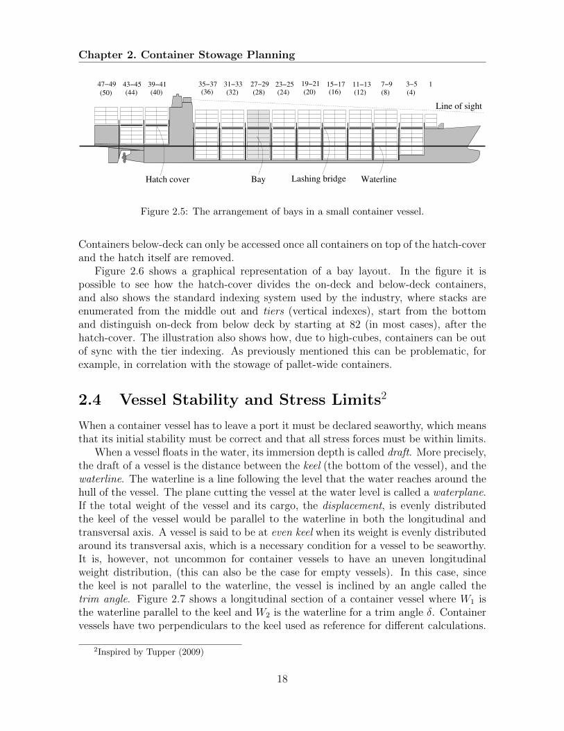
Figure 2.5: The arrangement of bays in a small container vessel.
Containers below-deck can only be accessed once all containers on top of the hatch-coverand the hatch itself are removed.
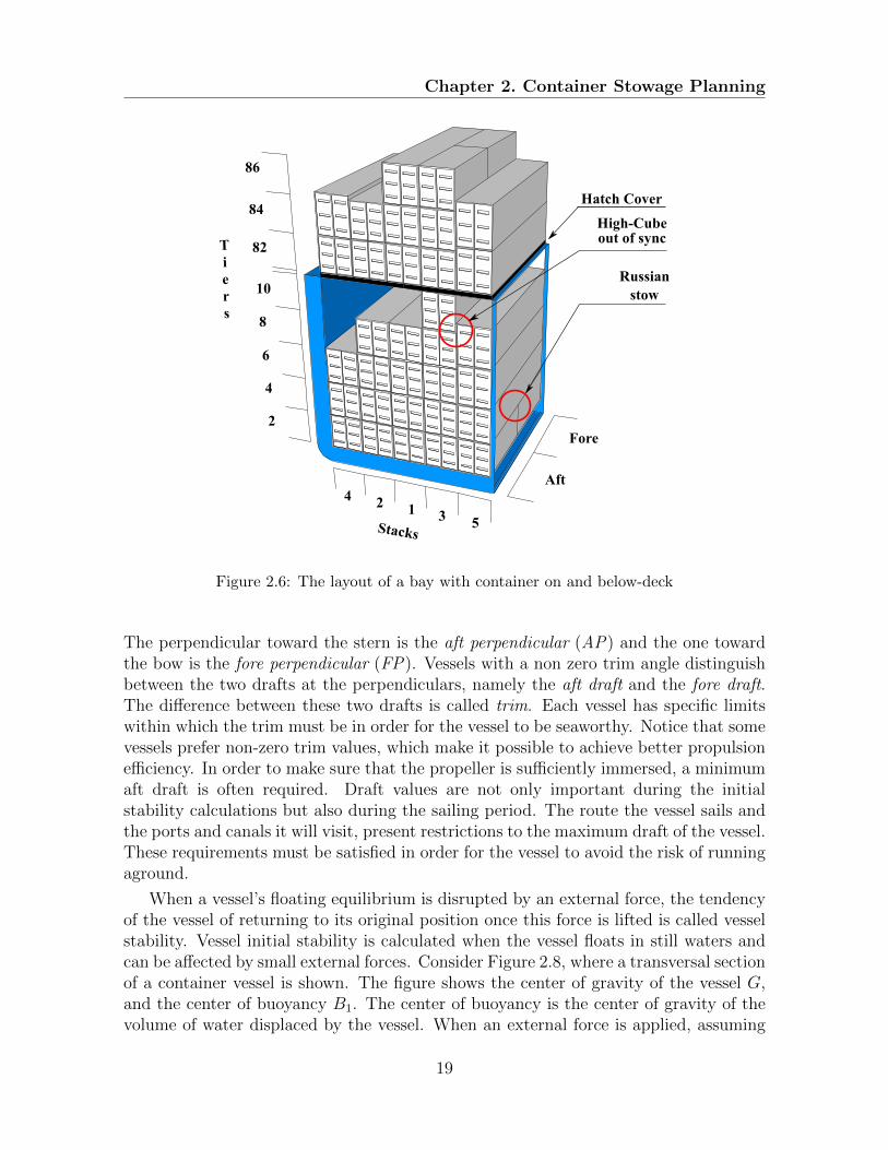
Figure 2.6 shows a graphical representation of a bay layout. In the figure it ispossible to see how the hatch-cover divides the on-deck and below-deck containers,and also shows the standard indexing system used by the industry, where stacks areenumerated from the middle out and tiers (vertical indexes), start from the bottomand distinguish on-deck from below deck by starting at 82 (in most cases), after thehatch-cover. The illustration also shows how, due to high-cubes, containers can be outof sync with the tier indexing. As previously mentioned this can be problematic, forexample, in correlation with the stowage of pallet-wide containers.
2.4 Vessel Stability and Stress Limits2
When a container vessel has to leave a port it must be declared seaworthy, which meansthat its initial stability must be correct and that all stress forces must be within limits.
When a vessel floats in the water, its immersion depth is called draft. More precisely,the draft of a vessel is the distance between the keel (the bottom of the vessel), and thewaterline. The waterline is a line following the level that the water reaches around thehull of the vessel. The plane cutting the vessel at the water level is called a waterplane.If the total weight of the vessel and its cargo, the displacement, is evenly distributedthe keel of the vessel would be parallel to the waterline in both the longitudinal andtransversal axis. A vessel is said to be at even keel when its weight is evenly distributedaround its transversal axis, which is a necessary condition for a vessel to be seaworthy.It is, however, not uncommon for container vessels to have an uneven longitudinalweight distribution, (this can also be the case for empty vessels). In this case, sincethe keel is not parallel to the waterline, the vessel is inclined by an angle called thetrim angle. Figure 2.7 shows a longitudinal section of a container vessel where W1 isthe waterline parallel to the keel and W2 is the waterline for a trim angle δ. Containervessels have two perpendiculars to the keel used as reference for different calculations.
2Inspired by Tupper (2009)
18
Chapter 2. Container Stowage Planning
Figure 2.6: The layout of a bay with container on and below-deck
The perpendicular toward the stern is the aft perpendicular (AP) and the one towardthe bow is the fore perpendicular (FP). Vessels with a non zero trim angle distinguishbetween the two drafts at the perpendiculars, namely the aft draft and the fore draft.The difference between these two drafts is called trim. Each vessel has specific limitswithin which the trim must be in order for the vessel to be seaworthy. Notice that somevessels prefer non-zero trim values, which make it possible to achieve better propulsionefficiency. In order to make sure that the propeller is sufficiently immersed, a minimumaft draft is often required. Draft values are not only important during the initialstability calculations but also during the sailing period. The route the vessel sails andthe ports and canals it will visit, present restrictions to the maximum draft of the vessel.These requirements must be satisfied in order for the vessel to avoid the risk of runningaground.
When a vessel’s floating equilibrium is disrupted by an external force, the tendencyof the vessel of returning to its original position once this force is lifted is called vesselstability. Vessel initial stability is calculated when the vessel floats in still waters andcan be affected by small external forces. Consider Figure 2.8, where a transversal sectionof a container vessel is shown. The figure shows the center of gravity of the vessel G,and the center of buoyancy B1. The center of buoyancy is the center of gravity of thevolume of water displaced by the vessel. When an external force is applied, assuming
19

Chapter 2. Container Stowage Planning
AP
FP
Draft AftDraft Fore
W1
W2 TrimTrim angle
δ
Figure 2.7: Longitudinal section of a vessel showing trim, draft and waterlines
constant displacement and no free weights, it is safe to assume that the rotation will notaffect the center of gravity, which thus remains constant. The center of buoyancy, onthe other hand, changes as the underwater volume changes its form. The gray wedgesbetween the original waterline W1 and the waterline after the inclination W2 representthe movement of the volume of water displaced by the vessel. The center of buoyancyof the vessel thus changes to B2. For small heeling angles (θ), it is safe to assume thatthe volume of the wedges will grow linearly with θ. The metacenter of the vessel isthe intersection M between the center line going through G and the center line goingthrough B2, and for small angles can be considered a fixed point. Once the externalforce inclining the vessel is removed an equal and opposite force δ will bring the vesselback to its original position. The perpendicular from G to B1M is called the rightinglevel (z), thus the moment with which the vessel rolls back to is original position isMr = δz = δGM sin θ, where GM is called the metacentric height. Vessels have aminimum required GM before they can be considered stable. The larger the GM themore stable the vessel is. Too large values might, however, result in too “stiff”a vessel.
The weight distribution on a container vessel does not only affect its stability; Theforces at play on a vessel stress its physical structure and must be kept within the vessel’sstructural limits. The most basic structural stresses are those regarding the weight ofthe container stacks, which must not exceed the maximum capacities. Nowadays shipsare designed to be light in order to reduce bunker consumption. It is thus important totake structural weight limitations into account. Two weight limits exist for each stack,one regarding the outer container supports and one regarding the inner supports. Limitson the inner supports are often the most stringent as the vessel structure in the middleof a stack is weaker. The inner supports are used only when 20’ containers are stowed.When 20’ and 40’ containers are mixed in the same stack, only half of the 20’ weight isconsidered to be supported by the outer supports, since the other half sits on the innersupports.
Other structural stresses come from the distribution of the upward and downwardforces that act on the vessel. When a body floats in still water, it experiences twoacting forces: a downward force due to gravity (the weight), and an equal and opposite(upward), force due to hydrostatic pressure. The upward force is the buoyancy andits magnitude is equal to the mass of water displaced by the object. This is also truefor container vessels. Even though the total weight and buoyancy forces are equal, the
20

Chapter 2. Container Stowage Planning
G
B1 B2
M
W1
W2
metacentric height
θ
δ
z
Figure 2.8: Transversal section of a vessel showing initial stability components.
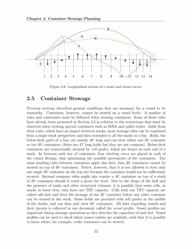
shape of the hull and the uneven distribution of weight results in an uneven distributionof forces along the vessel which stresses its structure. Each vessel has a fixed set ofcalculation points called frames for which stress limits are known. Consider Figure 2.9.It shows a longitudinal section of a container vessel with 14 frames. The W curverepresents the weight distribution along the vessel and the O curve is the correspondingbuoyancy. For each of the sections between each frame, the arrows denote the resultingforces acting on each section. Should each one of these sections be allowed to freelymove, sections with a stronger downward force will sink more into the water while theopposite would be true for those with stronger upward forces. Since the sections arenot allowed to move, they cause shearing and bending stresses over the vessel structure.The shear force on a vessel, at a specific frame, is the integral of the forces on eitherside of the frame. Similarly, the bending moment at each frame is the integral of themoments on either side of the frame; another way of seeing this is using the load curve,which shows the resulting force per length unit where moment is defined as force timesdistance. Shear force is then the area under the load curve, from either the bow or thestern to the frame of calculation. Shear force is shown in Figure 2.9 as the curve S.The image also shows the bending curve B for the bending moment of the vessel, whichcan also be computed as the area under the shear force curve S.
Modern container vessels are equipped with ballast tanks. These tanks can be usedto load water, and thus distribute extra weight along the vessel to, for example, im-prove vessel stability or adjust weight distribution to reduce stress forces. Automaticpumps can move water between the tanks, which is particularly useful during load anddischarge operations.
21
Chapter 2. Container Stowage Planning
1 2 3 4 5 6 7 8 9 10 11 12 13 14
B
OW
S
Figure 2.9: Longitudinal section of a vessel and stress curves.
2.5 Container Stowage
Previous sections described general conditions that are necessary for a vessel to beseaworthy. Containers, however, cannot be stowed on a vessel freely. A number ofrules and constraints must be followed when stowing containers. Some of these ruleshave already been presented in Section 2.2 in relation to the restrictions that must beobserved when stowing special containers such as IMOs and pallet-wides. Aside fromthese rules, which have an impact between stacks, most stowage rules can be explainedfrom a single stack perspective and then extended to all the stacks in a bay. Holds, thebelow-deck parts of a bay, are mainly 40’ long and can stow either one 40’ containeror two 20’ containers, (there are 45’ long holds but they are not common). Below-deckcontainers are transversally secured by cell guides, which are found on each end of astack. In between each tier of containers, four stacking cones are placed in each ofthe corner fittings, thus minimizing the possible movements of the containers. Thesame stacking rules between containers apply also here, thus 20’ containers cannot bestowed on top of 40’ containers. Notice, however, that it is not allowed to stow onlyone single 20’ container on the top tier because the container would not be sufficientlysecured. Internal company rules might also require a 40’ container on top of a stackof 20’ containers should it reach a given tier level. Due to the shape of the hull andthe presence of tanks and other structural volumes, it is possible that some cells, instacks in lower tiers, only have one TEU capacity. Cells with one TEU capacity arecalled odd-slots and force the stowage of one 20’ container before any other containercan be stowed in the stack. Some holds are provided with cell guides in the middleof the stacks, and can thus only stow 20’ containers. All data regarding vessels andtheir layouts is collected in one document called the vessel profile. Vessel profiles areimportant during stowage operations as they describe the capacities of each slot. Vesselprofiles can be used to check where power outlets are available, such that it is possibleto know where, for example, reefer containers can be stowed.
22

Chapter 2. Container Stowage Planning
Container stowage on-deck has the same basic stacking restrictions as in stowagebelow-deck. It is, however, uncommon to have Russian stacks, stacks of mixed 20’and 40’ containers, on-deck. Container stacks on-deck are not supported by the vesselstructure as the ones below-deck, thus containers must be secured in a different way.The stacking cones used below-deck are replaced by twist-locks, which similar to cones,fit into the corner castings, but that can lock containers between each other when thecone heads are twisted. Nowadays it is common to use automatic twist-locks whichrelease the containers automatically once a crane lifts them. The first two tiers ofcontainers are secured using lashing-rods. The use of lashing-rods presents, however,a restriction on the positioning of 20’ containers. Ship personnel must be able toreach in between two 20’ containers in order to tighten the lashing rods. Should a40’ container be stowed in the path of 20’ containers it would not be possible to lashthose last containers. All containers above the second tier, that cannot be lashed, areonly supported by the twist-locks. For that reason, stacks on-deck with more than twotiers must have at most a tier difference of one in order to support each other. Somevessels are equipped with a lashing bridge (see Figure 2.5), a metallic structure similarto the one found below-deck. Containers within the lashing bridge are firmly secured,and the bridge gives the possibility of lashing the next two tiers on top of it. In thatway, it allows much higher and secure stacking of containers. If a lashing bridge ispresent, it must be noted that long containers such as 45’ containers are only allowedabove the bridge. It is not allowed, even though physically possible, to stow 40’ on topof 45’ containers since the 40’ cannot be lashed. The rolling moment of a vessel alsoinfluences the way containers should be stacked on-deck in terms of security. Vesselshaving a short rolling period, and thus a large GM (see Section 2.4 for the definition ofGM ) experience strong forces on the top tiers. For that reason, it is preferable to havelight containers at the top of a stack and heavy at the bottom. If heavy containers areat the top, the resulting forces might collapse the entire stack. High container stackscannot be freely stowed on-deck due to wind forces. Shipping companies have differentwind-stacking rules. An example of such a rule is to not allow stacks to be more thanone tier higher than the ones supporting them on the side. The height that containerstacks can reach is also governed by the line-of-sight of the pilot house. The line-of-siteis a fictitious line from the pilot house to the sea at a distance equal to double the lengthof the vessel, or 500 meters, which ever is smallest. Containers are not allowed abovethis line or they will obstruct visibility, an example of which can be seen in Figure 2.5.
2.6 Stowage Plans
A stowage plan is an assignment of containers to slots in a vessel. Stowage plans aregenerated by stowage coordinators before a vessel reaches its destination port. Stowageplans are then used in the terminal to coordinate the load and discharge operations.Section 2.1 gave a description of the main costs of terminal operations, and mentionedthat those, and the tight schedule of liner vessels, result in a wish to minimize the time
23

Chapter 2. Container Stowage Planning
at port. It was already shown in Section 2.1 how the distribution of moves on each ofthe vessel’s bays has a direct impact on the crane-split and thus the total time thatterminal operations will take. Another, and very important, factor to the minimizationof time at port, is overstowage. Consider container a to be discharged in an arbitraryport, and container b to be discharged at a later port. Once the vessel reaches theport of discharge of container a, if container b is stowed on top of container a, b willneed to be discharged so that container a can be reached. Container b will then haveto be loaded again into the vessel to continue to its port of destination. Container bis said to overstow container a and the extra moves caused by this overstowage arecalled shifts. There also exists a more costly kind of overstowage, one that involveshatch-covers. Consider again container a, but this time assume it is stowed below-deck.Once container a has to be discharged, all the containers over the hatch-cover, that donot have the same discharge port as a, will be overstowing a independently of whichstack they are stowed in since it is necessary to remove the hatch-cover. All thesecontainers will result in shifts. Clearly, stowing containers with a later discharge portfirst will reduce this problem. However, such stowage would result in a horizontal layerdistribution of discharge ports which could have a disastrous impact on the stowageplans at later ports. It is for this reason, that stowage coordinators must take futureports into account when decisions about the stowage plans are taken. Normally stowagecoordinators have about six hours to produce a stowage plan. The information at theirdisposal is: a loadlist containing information (weight, size and discharge port), aboutthe containers to be loaded on the vessel, a release containing the same informationabout the containers already onboard the vessel, a forecast, based on historical data,giving information about the containers to be expected in down stream ports, and portdata about the string, such as the number of assigned cranes and port depths. Inorder to help stowage coordinators produce valid plans, they are often given access tospecialized software that can, in real time, calculate and give feed back on the stateof a vessel given a specific stowage plan. Stowage planning then becomes a complexpuzzle governed by expert guidelines, experience and the trial and error feed back of thecurrently available software packages. One of the most successful stowage guidelines isblock stowage. When block stowing, stowage coordinators attempt to assign dischargeports to sections of bays to minimize crane workloads and overstowage at current andfuture ports. The containers in the loadlist are then loaded within those blocks ifpossible. Stowage coordinators also use a number of rules-of-thumb that allow them toproduce robust plans, such as making sure that reefer plugs are correctly utilized suchthat they can be available when containers have to be stowed in future ports.
24
Chapter 3. Related Work
Chapter 3
Related Work
Previous academic work is rich with innovative solution approaches, but has been chal-lenged by the inaccessibility of the problem. This has led to limited representativepower of the developed models and a lack of test instances. The work can be clusteredinto two main groups: approaches based on a single model of the entire problem andapproaches based on a decomposition of the problem into several optimization models.Between the methods aiming at optimality, the latter approaches are the most success-ful, however, most of the work in the literature focuses on heuristic approaches using asingle model. To the best of the author’s knowledge, this chapter presents a completereview of the academic work for the container stowage problem.
3.1 Single Model Approaches
Mathematical Programming
Within the realm of single model optimization, mathematical modeling has been appliedby Ambrosino et al. (2004) and Li et al. (2008). Ambrosino et al. (2004) use a 0-1Integer Programming (IP) formulation that considers 20’ and 40’ containers withinthree weight classes. The model indirectly deals with lashing and GM constraints byforcing containers to be ordered descending by weight from the bottom to the top instacks. Containers with special requirements, such as reefers, are not modelled andoverstowage is modelled as a constraint rather than an objetive. The goal of the modelis to minimize time at port. Using a preprocessing procedure, the proposed IP modelcan solve stowage instances for a single vessel of 188 TEUs within 33 minutes on aPC Pentium II. The model, however, only considers the current port. Li et al. (2008)also propose a 0-1 IP model, but take a multi-port scenario into account. Similarto Ambrosino et al. (2004) only standard 20’ and 40’ containers are modelled. Thiswork, however, does not consider weight limitations but does represent overstowage asan objective. The authors claim to solve randomly generated problem instances for asingle vessel of 800 TEUs but present no details of the runtime results.
25
Chapter 3. Related Work
Placement Heuristics
Pure placement heuristics have been explored by Avriel et al. (1998) and Yoke et al.(2009). Avriel et al. (1998) presented the Suspensory Heuristic Procedure, which is re-stricted to a single bay vessel and solves the stowage problem of a single size containerwithout taking into account the stability of the vessel. The heuristic is aimed at mini-mizing overstowage in a multi-port problem where only loading is allowed. Randomlygenerated problem instances with vessels of up to 1,700 TEUs can be solved within 30seconds. In the same paper, the authors also present an IP model that can solve thisproblem to optimality for very small instances. Yoke et al. (2009) proposes a placementheuristic based on the work practice of stowage coordinators. Containers are initiallygrouped by discharge port, length, and type of special requirements. The vessel isthen partitioned in so called blocks to which discharge ports are assigned. After this,containers are stowed into each group using heuristic rules. These rules minimize over-stowage but do not embed stability considerations. The authors show evidence thatone problem instance for a single vessel of 5,000 TEUs can be stowed efficiently. Thefeasibility of the plan is, however, not guaranteed. Some improvements to the heuristicrules are presented by Fan et al. (2010) in order to take stability into account.
Placement Heuristics with Local Search
Some of the earliest work combines a placement heuristic with local search. Scott andChen (1978) propose grouping containers into classes based on special requirements,leaving the last class to hold all the standard containers which are then further classifiedaccording to their weight. Containers with special requirements are assigned to slotsfirst based on some heuristic rules. Two IP models are then solved, one to assign thestandard containers to bays and maximize intake, and one to optimize ship stability.A local search using container swaps as a neighborhood is used to solve the trim andGM . Should it not be possible to find a solution, the process is repeated by removingone container form the loadlist. The method does not take overstowage into accountand has long computation times according to the authors. Aslidis (1984) solved asimplified version of the problem with one size of container without special requirements.Overstowage minimization was the only objective and weight capacities were not takeninto account. The authors propose a placement heuristic for the containers where trimis solved using ballast water. A local search based on swap neighborhoods is used tosolve the GM . Once a feasible solution is found, swaps with no cost on the objectivevalue are performed to maximize GM . Two test cases on a 1,500 TEU vessel were solvedwithin 30 seconds. Similar ideas have recently been investigated by Liu et al. (2011)and Low et al. (2011). Low et al. (2011) improves the solutions given by the placementheuristic of Yoke et al. (2009) using a local search with swap neighborhoods that arespecifically designed to solve weight limits, trim, and heel requirements. The work ofLiu et al. (2011) modifies the heuristic of Yoke et al. (2009) to obtain non-deterministicsolutions. In a first stage the modified heuristic is used to generate a number of initialsolutions. The best of these, in terms of overstowage and crane intensity, are then used
26
Chapter 3. Related Work
in a second stage. The second stage uses a swap neighborhood limited to containerswith the same discharge port to solve the stability as a multi-objective problem. Forthe vessel of 5,000 TEUs examined by the authors, 10 non-dominant solutions can befound within 2,600 seconds.
Bin Packing Heuristic
The similarity between the stowage problem and the Bin Packing problem has beeninvestigated by Sciomachen and Tanfani (2003) and Zhang et al. (2005). Sciomachenand Tanfani (2003) adapt a 3D-Bin Packing heuristic to a stowage problem which takesinto account 20’ and 40’ containers and high-cube containers. The vessel is dividedinto sections that are filled by containers according to their destination and length.Main sections have simple forms and are easy to stow, while remaining sections areleft for later stowage. Stability and stacking constraints are considered in the loadingorder of containers and sections. Generated plans are designed for only one port. For avessel of 1,800 TEUs, the two industrial cases can be solved within 33 minutes. Zhanget al. (2005) propose a bin packing model of the multi-port stowage problem. Stabilityconstraints, however, are not modelled. Overstowage minimization and minimizationof the number of used bays are optimized by modeling the packing decisions as a binarydecision tree traversed using bin packing heuristics. One case study with a vessel of895 TEUs was presented but there was no accompanying runtime performance.
Genetic Algorithms
Dubrovsky et al. (2002) propose a compact encoding of a container stowage problemsimilar to that described by Avriel et al. (1998). In this encoding, a single bay ves-sel can be stowed with one size of container. Stability and container weights are nottaken into consideration. The solution process does, however, heuristically handle trimrequirements. Random problem instances, with vessels of 500 and 1,000 TEUs, havebeen solved for 10 ports in 30 minutes. Another work that makes use of genetic algo-rithms is that of Imai et al. (2006) where container stowage and terminal sequencingare combined. Sequencing is introduced by modelLing the transportation time neededfor each container to be retrieved from the yard. Plans are only produced for the holdsand overstowage is modeled as a constraint. Stability is taken into account as well asGM , trim, and heel angles. The algorithm, however, takes over 1 hour to generateplans for random problem instances of vessels in the range of 500-2,000 TEUs.
Constraint Programming
The use of Constraint Programming (CP) for container stowage was introduced by Am-brosino and Sciomachen (1998). In this work, a single bay vessel loading 350 containersis modelled. The approach takes 20’, 40’, and IMO containers into account, and hasa heuristic handling of the stability constraints. The CP model is optimized within abranch & bound framework where overstowage and intake are optimized. The model
27

Chapter 3. Related Work
also considers the use of Roll-On Roll-Off vessels. The authors claim to solve prob-lem instances within 10 minutes, but no evidence is presented. Later, Delgado et al.(2009) presented a different CP model which takes into account most of the stackingconstraints for vessel holds, but disregards IMO restrictions and stability. A detaileddescription of the model and its improvements, such as symmetry breaking, channel-ing constraints and partial evaluations are presented. An extension of this work waslater published (Delgado et al., 2012) where an in-depth comparison with an IP modelis shown. The approach can solve industrial problem instances of 100 TEUs vesselpartitions to optimality within 1 second, (in most cases). It must be noted that thismodel solves the slot planning problem of the decomposition described in this thesis,thus stability is assumed to be handled during the master planning phase. This is alsothe approach used to generate the optimal solutions for the evaluation of the CBLSalgorithm presented in this thesis.
Simulation
Simulation in stowage planning is found in one of the earliest (Shields, 1984) and oneof the latest (Azevedo et al., 2012) contributions. Shields (1984) uses a Monte Carlomodel with the aim of handling the uncertainty of cargo in the loadlists. For each port,container groups are loaded into the vessel using heuristic guidelines that try to pruneslots where the analysed containers cannot be stowed and thus aim to find bays thatcan stow the entire group. Penalty functions are used to rank solutions and the threebest ones are selected for each port. An overall best solution between all ports is thenselected. No performance results were published. Azevedo et al. (2012) uses simulationin a similar fashion, however, stochasticity is not taken into account. Azevedo et al.(2012) proposes a solution search based on the selection of the loading and unloadingrules applied by stowage coordinators. The idea is to decide which overall rules to use,and simulate them in order to generate a plan. The decision tree is then traversedusing beam search in order to reduce the search space. Stability and standard onesize containers (with unitary weight) are taken into account. The model optimizesoverstowage and stability with a runtime between 400 and 18,000 seconds for a 1,500TEU vessel.
Other Approaches
Giemsch and Jellinghaus (2004) present an alternative approach to the uncapacitatedsingle bay problem, where a 2-step heuristic stows containers by their discharge portsinto stacks. The remaining containers, those for which a stack that does not force re-handles cannot be found, are assigned to slots using a branch & bound search. Theauthors claim to achieve better results than the Suspensory Heuristic Procedure byAvriel et al. (1998), but no detailed results have been published. The same problemis solved by Yanbin et al. (2008) using a multi-agent system, which, however, onlyachieves results comparable to those of the Suspensory Heuristic Procedure. Nugroho
28
Chapter 3. Related Work
(2004) presents a very different approach, a case-based system. The idea is to find astowage plan similar to the one in question within a knowledge base. The databaseof cases will then grow and be more accurate the more stowage plans are solved. Nosufficient experimental evaluation of the idea is presented.
3.2 Decomposition Models
To the best of the author’s knowledge, the first decomposition of the stowage problemwas proposed by Botter and Brinati (1992). In this work, a detailed mathematical modelof the container stowage problem was presented. The model also included decisions overthe sequence in which containers should be loaded or discharged. Botter and Brinati(1992) proposed to solve the problem using a decomposition which first solves theassignment problem of containers to slots, and then the sequencing problem. Given asolution to the assignment problem, the set of sequencing variables was greatly reduced.The decomposition, however, was too computationally expensive and was replaced bya branch & bound search with domain specific branching heuristics. The authors claimthat the search could be stopped within acceptable computational times and result ingood quality stowages. No evidence of these results was presented.
The first decomposition approach that presented promising results was the work ofWilson and Roach (1999)(Wilson and Roach, 2000; Wilson et al., 2001) where the blockbased decomposition was introduced. Wilson and Roach (1999) divided each bay of thevessel into blocks. Blocks are logically distributed such that they are either on or below-deck and often follow the pattern of the hatch covers. The proposed decomposition firstsolves an assignment problem from container groups to blocks. This problem is solvedusing an enumeration algorithm where solutions are graded by a fitness function. Thealgorithm optimizes overstowage, crane utilization, and discharge port clustering withinblocks. Given this assignment, a tabu search is run to find the assignment of containerswithin each block. Here overstowage is minimized, container weights are ordered, andstacks with the same discharge port are preferred. Without presenting any evidence,the authors claim to solve problem instances for 688 TEU vessels. A total of 90 minutesis necessary for the block assignment problem, and less than 1 hour for the tabu searchto be completed.
Kang and Kim (2002) presented an iterative decomposition, where information ispassed between the master and the sub-problem. Kang and Kim (2002) have alsoadapted the concept of block decomposition, and, as with Wilson and Roach (1999),the first stage of the decomposition assigns container groups to blocks. Only one sizeof container with no special requirements is taken into consideration. The assignmentproblem is not solved for all ports simultaneously but for one port at a time with theobjective of reducing overstowage and stability violations. Solutions are found usinga modified version of the transportation simplex that uses specialized pivoting rules.The classes of containers are then assigned to the slots using a tree search enumerationfor each block. After this, information from the slot assignment is passed to the block
29
Chapter 3. Related Work
assignment algorithm in order to find improving solutions. The approach can solverandomly generated problem instances for 4,000 TEU vessels using three weight classesfor the containers in 640 seconds, while planning for eight ports.
A different decomposition approach is proposed by Ambrosino et al. (2006) that isbased, however, on the assumption that overstowage is a hard constraint in the model.The authors present a 3-phase decomposition. In the first phase, containers are groupedaccording to their discharge port and are distributed among the bays (which are devotedto one discharge port) taking into account capacities. For each defined partition of thevessel, an IP model is solved that assigns containers to specific slots. Once all partitionsare solved, a local search uses a swap neighborhood to improve the stability of the vessel.The approach generates stowage plans for a single port, and with a vessel of 198 TEUs,it runs in 3.5 minutes and finds solutions with a one percent optimality gap comparedto the IP model of Ambrosino et al. (2004). Later, the authors propose a modificationof the decomposition (Ambrosino et al., 2009) where a new IP model for the solutionof the single destination partitions is presented and the simple local search is changedto a tabu search. The new modifications allow the decomposition to scale up to a 2,124TEUs vessel with a runtime of 74.7 seconds. Further research on the decompositionmodel was presented by Ambrosino et al. (2010), where a constructive heuristic wasdeveloped and used after the initial bay assignment. The heuristic is based on AntColony Optimization where the first decision is the assignment of containers to stacksand the successive decision is the assignment of containers to slots. The found solutionis then improved using local search. The ant system is updated (pheromone update)and a solution is returned once the ants start converging. The new heuristic was shownto solve problem instances for a 5,632 TEU vessel in 139.4 seconds. Multi-port solutionsand overstowage have not yet been modeled.
Gumus et al. (2008) presents a multistage decomposition, where containers aregrouped into types. In the first stage, fractions of bay capacities are assigned to specificdischarge ports. The assignment is then refined at the tier level such that hatch coverscan be taken into account. Then, further refinement is made at the slot level. Thefourth, and last, stage assigns containers to the slots according to the assigned portof discharge and uses a heuristic to handle vessel stability. Aside from the first stage,solved with a mixed-integer program, the authors do not provide details of the otherstages. The decomposition is claimed to scale to large instances but no evidence hasbeen presented.
30
Chapter 4. Representative Problem and Algorithmic Framework
Chapter 4
Representative Problem andAlgorithmic Framework
Chapter 2 gave an in-depth overview of all the details and constraints that surroundthe container stowage problem. From a research point of view, it would be unpracticalto study models of the problem that include all those details. Instead we propose tostudy a representative problem. This problem should include all the core computationalcomponents of the container stowage problem, and, at the same time, be detailed enoughfor the industry to be able to evaluate the value of the obtained results.
4.1 A Representative Problem
The definition of a representative problem requires balanced decisions about whichparts of the original problem should be relaxed and which should be always taken intoaccount.
4.1.1 Container Types
The computational complexity of the container stowage problem does not depend on thetype of containers used, as the assignment problem itself is nontrivial (see Appendix A).Such an observation could lead to the representation of only one container type. Stowagecoordinators, however, know that it also can be hard to find stowage plans where 20’and 40’ containers are mixed. This is due to the fact that 20’ containers cannot bestowed on top of 40’ containers and that the vessel arrives non-empty. For this reason arepresentative model should at least include containers of these two length’s. Containerswith other lengths are not very common, with exception of the 45’ containers which,however, are not involved in complex constraints.
Containers with special requirements, such as reefers, IMO, OGG and pallet-wides,can also have a significant impact on the complexity of the problem. Pallet-wides aregenerally used on specific routes and thus are not representative of the general problem.OGGs, such as bulk cargo, are not very common and one can imagine them as being
31
Chapter 4. Representative Problem and Algorithmic Framework
handled by the stowage coordinator and thus simply resulting in a capacity reduction.The same can be said about IMO containers since vessels often have dedicated baysfor those containers towards the bow. One could easily imagine models where IMOsare forced to be stowed on such bays and where the final decision of their positioningis left to the stowage coordinators. Reefer containers are more common, and representan everyday challenge for stowage coordinators. Due to the fact that vessels have alimited number of reefer plugs, the positioning of those containers can greatly influencea stowage plan. For this reason a representative stowage problem should include reefercontainers. It is debatable whether high-cube containers should be included into arepresentative problem. It is true that the extra height of those containers might leadto a reduction in the capacity of a vessel, but at the same time from a computationalstand point they can be seen as extra capacity constraints, and thus redundant from acomputational perspective.
4.1.2 Vessel Layout and Routes
Considering the shape of the vessel is important for solving the container stowage prob-lem as it posts major constraints on the possible distribution of containers. Also fromthe perspective of the industry, it would be very hard to evaluate solutions based onrectangular vessels, as there would be a good chance that the produced stowage planswill not look anything like the ones stowage coordinators are used to seeing. For astowage problem to be representative it should consider the layout of the vessel, in-cluding the separation between on and below-deck with hatch covers. A problem whichdoes not take hatch covers into account cannot model the hatch-overstowage, which isa significant part of the overstowage calculation. We, however, do not regard odd-slots(cells that only allow the stowage of one TEU) as part of the representative problemsince it would only result in extra capacity constraints that do not have an impact onthe computational complexity of the problem or on the way stowage coordinators wouldevaluate the results.
Vessels should also be considered to have an initial load of containers. This initialload forces stowage plans toward specific configurations, which is a property that shouldbe exploited from a computational point of view. Moreover, a stowage problem thatincludes already onboard containers is more representative of the everyday planning thata stowage coordinator has to perform. All ports of the plan should also be considered.Besides the fact that stowage coordinators judge stowage plans also on their robustness,a multiport problem has a higher level of complexity which cannot be ignored.
4.1.3 Vessel Stability
It is clear that the stability of the vessel is of high importance for the industry, andthus automated stowage plans should be as accurate as possible in that regard. Stowageplans that do not take stability into account, or that are too inaccurate, might forcestowage coordinators to make big changes to the plan, which defeats the purpose of
32
Chapter 4. Representative Problem and Algorithmic Framework
solving the problem. To give an example, due to the shape of the vessel it can behard to handle bending moments as there is not enough capacity at the extremities ofthe vessel. A solution to a container stowage problem that disregards bending mightrequire the stowage coordinator to change its container distribution such that less weightis assigned at the vessel’s extremities. With regard to stress forces and ship stability,ballast water can have a significant impact as well. Since the release of ballast water canhave significant environmental impacts, it is debatable whether the amount of waterin the tanks will change drastically within a stowage planning horizon. Nevertheless,a representative stowage planning problem should at least take the weight distributionof the water into account.
4.1.4 Container Stowage
Clearly, basic container stacking rules should be part of the representative problem.Vessels tend to be loaded close to their maximum capacities. When combining thisfact with the optimized construction of the vessels, it is clear that it is not possibleto disregard the structural limitations of a ship such as the weight constraints of thestacks. Due to the presence of hatch-covers and the requirement for line-of-sight, itis also unreasonable to model problems that consider uncapacitated stacks. Represen-tative models should also consider on-deck wind stacking rules (at least heuristically),since inter-bay container arrangements can be restrictive, especially in the cases wherecontainers with different discharge ports are stowed in the same bay.
4.1.5 Container Stowage Objectives
Overstowage has the largest impact on the efficiency of a stowage plan as it resultsin extra moves. Any representative model should include overstowage both for thecurrent and down-stream ports. It is also important to include hatch overstowagein the objective calculation due to the significant number of extra moves that it couldenforce. Different ways of defining crane utilization exist, and those ways are most likelycompany and contract dependent. One thing that is common is that the arrangement ofcontainers in a vessel will be heavily affected by it, thus a representative model should insome way take those concepts into account. Ballast water minimization is often requiredfor optimizing bunker consumption. As previously mentioned, releasing ballast watercan have environmental consequences thus it is possible that only a limited amountof water can be released. For that reason we do not believe that ballast optimizationshould be part of the representative problem. The handling of the current conditionof the tanks should, however, still be taken into consideration. When discussing withstowage coordinators, one can find a large number of characteristics that each stowagecoordinator thinks a stowage plan should have. We believe that such considerations,can be left out of a representative model.
33
Chapter 4. Representative Problem and Algorithmic Framework
4.1.6 The Proposed Problem
In summary, we propose the following representative container stowage problem.
Definition 1. Given a vessel profile that includes hydrostatic data, capacity and layoutof bays, and given data about the ports in the planned route including a loadlist ofcontainers at the current port and a forecast for the containers in the down-streamports, generate a stowage plan for the containers in the loadlist such that:
1. Both 20’ and 40’ containers are modelled
2. Reefer containers are stowed near power plugs
3. Already onboard containers are considered
4. Container stacking constraints are satisfied
5. Stack weight and height limits are respected
6. Trim, heel, draft and GM are within limits
7. Shear forces and bending moments are within limits
8. Wind stacking rules are taken into account
9. Loading and discharge of containers is allowed for all planned ports
The generated stowage plans should then minimize overstowage, hatch overstowage, andmaximize crane utilization.
4.2 The Quad Framework
The work in this thesis is part of a research project that uses an algorithmic frameworkcalled Quad. This framework assumes a block decomposition similar to that of Wilsonand Roach (1999) and Kang and Kim (2002). The problem is decomposed into a masterplanning problem and a slot planning problem. During master planning we solve theproblem of distributing groups of containers to sub-sections of bays called locations. Thecontainers are grouped based on their weight, length, and special requirements, (e.g.reefers). In order to achieve a robust plan, the framework assumes that the masterplanning problem is solved for the current port and a number of down-stream ports.The input of master planning is thus the loadlist of the current port and a forecast ofthe containers to be transported in the future ports. The input also includes the vesselprofile and data about the ports the stowage is planned for, (e.g. maximum draft,cranes available, etc.). It is in this phase that stability constraints are handled andthe hatch-overstowage and crane utilization are optimized. The output of the masterplanning phase is an assignment of container groups to locations for the current port,
34
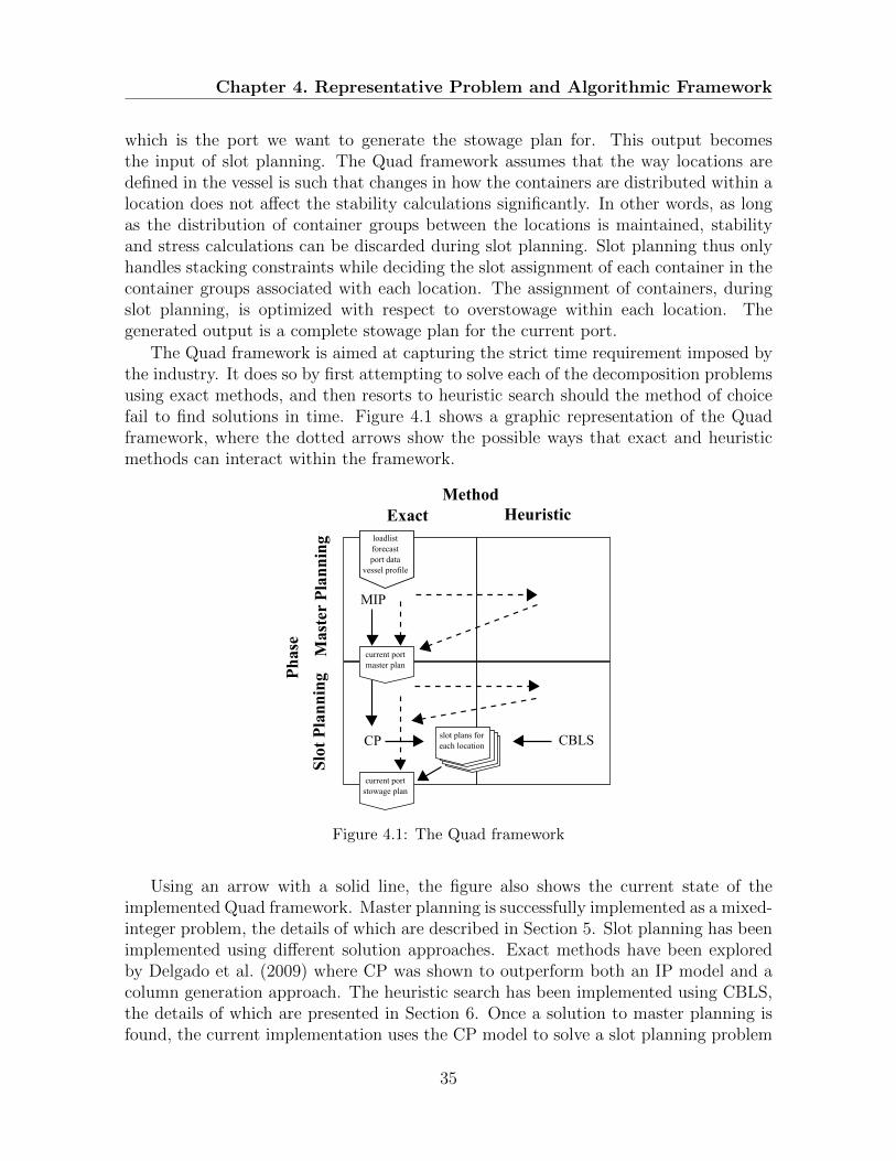
Chapter 4. Representative Problem and Algorithmic Framework
which is the port we want to generate the stowage plan for. This output becomesthe input of slot planning. The Quad framework assumes that the way locations aredefined in the vessel is such that changes in how the containers are distributed within alocation does not affect the stability calculations significantly. In other words, as longas the distribution of container groups between the locations is maintained, stabilityand stress calculations can be discarded during slot planning. Slot planning thus onlyhandles stacking constraints while deciding the slot assignment of each container in thecontainer groups associated with each location. The assignment of containers, duringslot planning, is optimized with respect to overstowage within each location. Thegenerated output is a complete stowage plan for the current port.
The Quad framework is aimed at capturing the strict time requirement imposed bythe industry. It does so by first attempting to solve each of the decomposition problemsusing exact methods, and then resorts to heuristic search should the method of choicefail to find solutions in time. Figure 4.1 shows a graphic representation of the Quadframework, where the dotted arrows show the possible ways that exact and heuristicmethods can interact within the framework.
Method
Exact Heuristic
Ph
ase M
ast
er P
lan
nin
gS
lot
Pla
nn
ing
MIP
CP CBLS
loadlist
forecast
port data
vessel profile
current port
master plan
current port
stowage plan
slot plans for
each location
Figure 4.1: The Quad framework
Using an arrow with a solid line, the figure also shows the current state of theimplemented Quad framework. Master planning is successfully implemented as a mixed-integer problem, the details of which are described in Section 5. Slot planning has beenimplemented using different solution approaches. Exact methods have been exploredby Delgado et al. (2009) where CP was shown to outperform both an IP model and acolumn generation approach. The heuristic search has been implemented using CBLS,the details of which are presented in Section 6. Once a solution to master planning isfound, the current implementation uses the CP model to solve a slot planning problem
35

Chapter 4. Representative Problem and Algorithmic Framework
for each location. The CBLS model is used in all the cases where the CP model failsto find solutions. The mixed-integer programming model for master planning and theCBLS model for slot planning are part of the work behind this thesis.
36
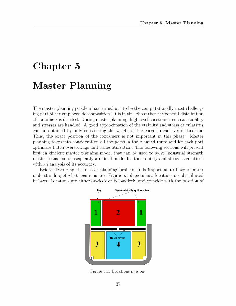
Chapter 5. Master Planning
Chapter 5
Master Planning
The master planning problem has turned out to be the computationally most challeng-ing part of the employed decomposition. It is in this phase that the general distributionof containers is decided. During master planning, high level constraints such as stabilityand stresses are handled. A good approximation of the stability and stress calculationscan be obtained by only considering the weight of the cargo in each vessel location.Thus, the exact position of the containers is not important in this phase. Masterplanning takes into consideration all the ports in the planned route and for each portoptimizes hatch-overstowage and crane utilization. The following sections will presentfirst an efficient master planning model that can be used to solve industrial strengthmaster plans and subsequently a refined model for the stability and stress calculationswith an analysis of its accuracy.
Before describing the master planning problem it is important to have a betterunderstanding of what locations are. Figure 5.1 depicts how locations are distributedin bays. Locations are either on-deck or below-deck, and coincide with the position of
1 2 1
3 34
Symmestrically split location
Hatch covers
Bay
Figure 5.1: Locations in a bay
37

Chapter 5. Master Planning
the hatch-covers, which makes it easier to model hatch overstowage. Some locations arenot composed of a continuous row of stacks. This is the case of locations representingthe extremities of a bay. This split and symmetric distribution of stacks is a useful toolfor the modelling of the transversal stability. With the assumption that containers andtheir weights are symmetrically distributed in the locations, it is possible to disregardstability constraints about the heel angle.
5.1 A Model for Master Planning
The master planning problem described in this thesis considers both 20’ and 40’ con-tainers. As an example of containers with special requirements, reefer containers arealso considered. Containers are grouped into types and are assigned to locations. Loca-tions are then used as basic elements for the stability and stress calculations. We modeltrim, GM , draft, and shear forces as an example of stresses. Assuming that stackingconstraints are handled during slot planning, this model only lacks the handling of thebending moment and the wind-stacking rules compared to the representative problemdescribe in Chapter 4. Ballast tanks are included in the calculations, but are consideredconstants. Thus it is debatable to consider them as part of the problem.
More formally, master planning assigns container types to locations. For 20’ and40’ containers, we consider a set of four mutually exclusive container types T ={L,H,RL,RH}, respectively light and heavy containers and light and heavy reefercontainers. To produce a robust plan, our model takes into account the current and aset of down-stream ports P . We define transports TR as a set of pairs 〈p1, p2〉, wherep1, p2 ∈ P are the load and discharge port of a container type. Notice that the containertypes T are only a classification and thus are not bound to fixed weight ranges. Foreach type τ ∈ T , the average weight of the containers on a specific transport t ∈ TRis calculated and represented by the constants W 20τ
t and W 40τt . This results in a more
refined weight categorization than taking the average weight of the containers in eachcontainer class. We define two sets of decision variables x20τtl and x40τtl representing re-spectively the number of 20’ and 40’ containers of type τ ∈ T to be stowed on locationl ∈ L during transport t ∈ TR, where L is the set of all locations. Following is theproposed IP model:
minimize∑p∈P
∑l∈L
(COyOpl + CPyPpl + CRyRpl
)+∑p∈P
CTyTp (5.1)
subject to∑t∈TRON
p
∑τ∈T
(x20τtl + 2x40τtl
)≤ Cpl ∀p ∈ P, l ∈ L (5.2)
38
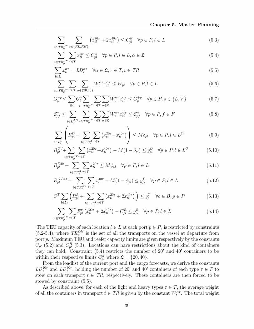
Chapter 5. Master Planning
∑t∈TRON
p
∑τ∈{RL,RH}
(x20τtl + 2x40τtl
)≤ CR
pl ∀p ∈ P, l ∈ L (5.3)
∑t∈TRON
p
∑τ∈T
xατtl ≤ Cαpl ∀p ∈ P, l ∈ L, α ∈ L (5.4)
∑l∈L
xατtl = LDατt ∀α ∈ L, τ ∈ T, t ∈ TR (5.5)∑
t∈TRONp
∑τ∈T
∑α∈{20,40}
Wατt xατtl ≤ Wpl ∀p ∈ P, l ∈ L (5.6)
G−ρp ≤∑l∈L
Gρl
∑t∈TRON
p
∑τ∈T
∑α∈L
Wατt xατtl ≤ G+ρ
p ∀p ∈ P, ρ ∈ {L, V } (5.7)
S−pf ≤∑l∈LAftf
∑t∈TRON
p
∑τ∈T
∑α∈L
Wατt xατtl ≤ S+
pf ∀p ∈ P, f ∈ F (5.8)
∑i∈LUl
RDpi +
∑t∈TRAp
∑τ∈T
(x20τti +x40τti
) ≤Mδpl ∀p ∈ P, l ∈ LO (5.9)
ROVpl +
∑t∈TROV
p
∑τ∈T
(x20τtl +x40τtl
)−M(1− δpl) ≤ yOpl ∀p ∈ P, l ∈ LO (5.10)
RD20pl +
∑t∈TRAp
∑τ∈T
x20τtl ≤Mφpl ∀p ∈ P, l ∈ L (5.11)
ROV 40pl +
∑t∈TROV
p
∑τ∈T
x40τtl −M(1− φpl) ≤ yPpl ∀p ∈ P, l ∈ L (5.12)
CT∑l∈Lb
(RApl +
∑t∈TRAp
∑τ∈T
(x20τtl + 2x40τtl
) )≤ yTp ∀b ∈ B, p ∈ P (5.13)
∑t∈TRON
p
∑τ∈T
F τpl
(x20τtl + 2x40τtl
)− CR
pl ≤ yRpl ∀p ∈ P, l ∈ L (5.14)
The TEU capacity of each location l ∈ L at each port p ∈ P , is restricted by constraints(5.2-5.4), where TRON
p is the set of all the transports on the vessel at departure fromport p. Maximum TEU and reefer capacity limits are given respectively by the constantsCpl (5.2) and CR
pl (5.3). Locations can have restrictions about the kind of containersthey can hold. Constraint (5.4) restricts the number of 20’ and 40’ containers to bewithin their respective limits Cα
pl where L = {20, 40}.From the loadlist of the current port and the cargo forecasts, we derive the constants
LD20τt and LD40τ
t , holding the number of 20’ and 40’ containers of each type τ ∈ T tostow on each transport t ∈ TR, respectively. These containers are then forced to bestowed by constraint (5.5).
As described above, for each of the light and heavy types τ ∈ T , the average weightof all the containers in transport t ∈ TR is given by the constant Wατ
t . The total weight
39
Chapter 5. Master Planning
of a location is then calculated and kept within its maximum limit Wpl (reflecting vesselcapacities), by constraint (5.6).
Hydrostatic data, specific to each vessel, is used to calculate its trim, draft, buoyancyand stability. Those calculations can be expressed as functions of displacement andcenter of gravity of the vessel. Due to our assumption about constant displacement(since no ballast can be added), hydrostatic calculations only depend on the center ofgravity of the vessel. This allows us to transform the stability, trim and draft restrictionsto bounds on the center of gravity. In constraint (5.7), for each port p ∈ P , the centerof gravity limits, G+ρ
p and G−ρp , have been calculated, where ρ ∈ {L, V } represent thelongitudinal and vertical components. The center of gravity of each location is definedby the constant Gρ
l . Due to the symmetrical position of the stacks in outer locations, itis possible to distribute the weight of the containers in these stacks such that the vesselis at even keel. For that reason we do not need specific constraints to ensure this.
Given a set of frames f ∈ F , where each frame is a calculation point as describedin Chapter 2, constraint (5.8) calculates the downward force created by the cargo aftof each frame f , where LAftf is the set of locations aft of frame f , and S+
pf and S−pf arethe maximum and minimum shear limits at frame f ∈ F for port p ∈ P , respectively.Since the weight of the vessel is constant, we pre-compute the buoyancy forces and thusonly restrict the weight distribution over the vessel accordingly.
Constraints (5.9 - 5.14) define the various objective components minimized in (5.1).A major objective is to minimize hatch-overstowage. This is modelled by the binaryvariables δpl ∈ {0, 1}, indicating the presence of containers to load or unload at portp ∈ P under on-deck locations LO. This is accomplished with constraint (5.9), whereLUl is the set of locations under l ∈ LO, TRA
p is the set of transports that are eitherloaded or unloaded in port p (we refer to such containers as active containers), and RD
pi
are the containers already on board the vessel when arriving at the first port (hereafterreferred to as the release), that are discharged from location i in port p. In constraints5.9-5.12) we make use of a BigM constant M . In our implementation of the model wetighten these constants to the upper bounds of the constraints. Variable yOpl is definedin (5.10) to be the number of hatch-overstowing containers in an on deck location l inport p given the set of transports TROV
p (and release containers ROVpl ), that overstow
containers to load or unload in port p.
Overstowage can happen also within locations. One of the major constraints thatcan force overstowage within a location is the fact that 20’ containers cannot be stowedover 40’ containers. Having many 20’ containers with earlier discharge ports than the40’ containers stowed in a location is thus an undesirable configuration. An estimateof the potential overstowage between 20’ and 40’ containers within each location isdefined by constraints (5.11) and (5.12). Constraint (5.11) introduces a new set ofBoolean variables φpl for each port p ∈ P and location l ∈ L, indicating the presence of20’ containers to load or unload. These indicator variables define the cost variable yPplin constraint (5.12). This variable holds the number of potential overstows between 40’and 20’ containers within a location. The constants RD20
pl and ROV40pl are the number of
containers in the release discharged and potentially overstowing in port p, respectively.
40

Chapter 5. Master Planning
Another important objective is the optimization of crane utilization. In this work,we define crane utilization as the makespan of the quay-side operations, in other wordsthe total amount of time needed for the cranes to perform all the load and dischargeoperations. Given that any two cranes must work at least two bays apart, we know thatcrane moves in adjacent bays can only be carried out by a single crane at a time. Thus,a lower bound of the makespan of cranes is the maximum work time for a single craneover the set of moves in adjacent bays, and this is the objective considered in this work.In the crane split example shown in Figure 2.2 this lower-bound would correspond to123 moves. Constraint (5.13) represents this calculation, where the variable yTp definesthe lower bound for each port p ∈ P . The index set B represents the set of adjacentbays. Lb is the set of locations of the pair of adjacent bays b ∈ B, RA
pl is the number ofactive TEU in location l and port p, and CT is the average time needed to move oneTEU by a crane.
During master planning, stacking rules are not taken explicitly into account. Forthat reason some generated slot planning instances may be infeasible. A possible sourceof this infeasibility is the reefer containers, since they can only be stowed in slots withpower plugs,(which might be occupied by other containers). Constraint (5.14) alleviatesthis issue by reducing the maximum capacity of reefer containers within a location bya proportional factor F τ
pl, where F τpl = CR
pl/Cpl for all non-reefer containers and a factor1 for all reefer containers. The reduction is then captured in the variable yRpl.
The master planning problem is, due to preference objectives such as reefer capacityreductions, strictly a multi-objective optimization problem. We, however, minimize aweighted sum of the cost variables where the weights (CO, CP , CR, CT ), correspond tothe preferences of our industrial partner and of stowage coordinators.
5.2 Complexity of the Master Planning Problem
From a bin-packing reduction, it is easy to show that slot planning is NP-Hard, (e.g.Sciomachen and Tanfani (2003)). The same reduction, however, does not apply to themaster planning problem since it abstracts the slots away. Here we show that masterplanning nevertheless is NP-Hard by a reduction from the Hatch Overstow Problem(HOP). A HOP instance is a tuple 〈C, in, out , H, r,m, k〉, where C is a set of containersand each container c ∈ C is loaded at port in(c) and discharged at port out(c), H isa set of hatch covers where each h ∈ H must be lifted in the set of ports r(h), and mis the capacity of each stowage area above a hatch cover. The question is whether it ispossible to stow all the containers with at most k hatch overstows in the stowage areaabove the hatches. The HOP is shown to be NP-Complete in Appendix A.4.
Proposition 1. Master planning is NP-Hard.
Proof. We reduce HOP to master planning by creating a vessel with 2|H| locations suchthat for each on deck location there is a corresponding counterpart below deck. Theset C of containers are created as 40’ reefer containers, where c ∈ C has load port in(c)
41
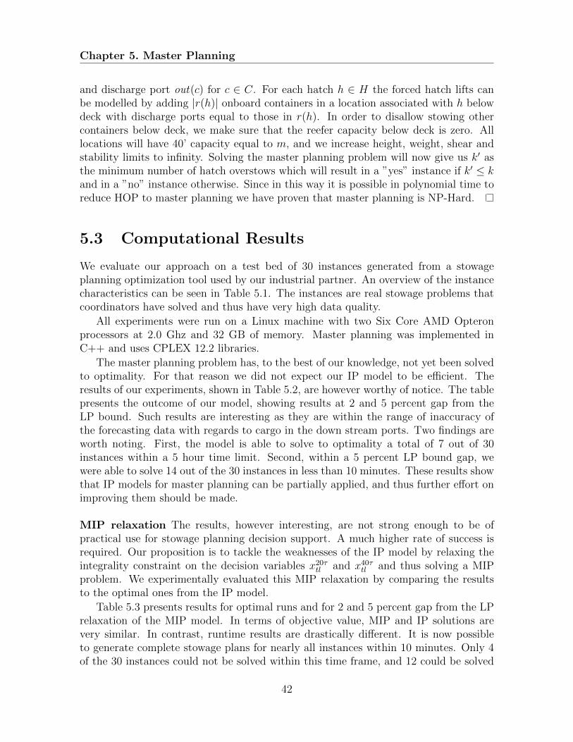
Chapter 5. Master Planning
and discharge port out(c) for c ∈ C. For each hatch h ∈ H the forced hatch lifts canbe modelled by adding |r(h)| onboard containers in a location associated with h belowdeck with discharge ports equal to those in r(h). In order to disallow stowing othercontainers below deck, we make sure that the reefer capacity below deck is zero. Alllocations will have 40’ capacity equal to m, and we increase height, weight, shear andstability limits to infinity. Solving the master planning problem will now give us k′ asthe minimum number of hatch overstows which will result in a ”yes” instance if k′ ≤ kand in a ”no” instance otherwise. Since in this way it is possible in polynomial time toreduce HOP to master planning we have proven that master planning is NP-Hard.
5.3 Computational Results
We evaluate our approach on a test bed of 30 instances generated from a stowageplanning optimization tool used by our industrial partner. An overview of the instancecharacteristics can be seen in Table 5.1. The instances are real stowage problems thatcoordinators have solved and thus have very high data quality.
All experiments were run on a Linux machine with two Six Core AMD Opteronprocessors at 2.0 Ghz and 32 GB of memory. Master planning was implemented inC++ and uses CPLEX 12.2 libraries.
The master planning problem has, to the best of our knowledge, not yet been solvedto optimality. For that reason we did not expect our IP model to be efficient. Theresults of our experiments, shown in Table 5.2, are however worthy of notice. The tablepresents the outcome of our model, showing results at 2 and 5 percent gap from theLP bound. Such results are interesting as they are within the range of inaccuracy ofthe forecasting data with regards to cargo in the down stream ports. Two findings areworth noting. First, the model is able to solve to optimality a total of 7 out of 30instances within a 5 hour time limit. Second, within a 5 percent LP bound gap, wewere able to solve 14 out of the 30 instances in less than 10 minutes. These results showthat IP models for master planning can be partially applied, and thus further effort onimproving them should be made.
MIP relaxation The results, however interesting, are not strong enough to be ofpractical use for stowage planning decision support. A much higher rate of success isrequired. Our proposition is to tackle the weaknesses of the IP model by relaxing theintegrality constraint on the decision variables x20τtl and x40τtl and thus solving a MIPproblem. We experimentally evaluated this MIP relaxation by comparing the resultsto the optimal ones from the IP model.
Table 5.3 presents results for optimal runs and for 2 and 5 percent gap from the LPrelaxation of the MIP model. In terms of objective value, MIP and IP solutions arevery similar. In contrast, runtime results are drastically different. It is now possibleto generate complete stowage plans for nearly all instances within 10 minutes. Only 4of the 30 instances could not be solved within this time frame, and 12 could be solved
42

Chapter 5. Master Planning
Instances Characteristics
ID Vessel Route EncodingCap. Loc. Ports Util. Weight Loadlist & Release Moves Transports Bools
(TEU) (%) (%) forecast
1 5802 58 7 58 56 11194 0 8163 16 4252 9112 100 7 80 65 27648 1515 26801 11 4503 9112 100 7 80 65 27648 1515 26801 11 4504 9882 87 7 66 65 14102 1438 16331 14 4485 5802 58 8 52 21 10268 1545 12988 18 4086 9078 100 10 65 48 39936 1409 26207 20 5717 8334 80 11 58 40 14862 2743 26702 37 6078 2480 40 8 42 38 4444 388 5130 20 2499 9958 87 8 58 51 15037 1741 16332 19 58510 3354 47 7 40 36 5717 139 5108 13 26711 2480 40 6 61 55 5306 191 5937 11 13712 3354 47 5 36 11 1831 111 3036 7 18213 8434 100 6 69 58 22127 525 9121 4 35014 7474 90 6 83 86 16985 1956 23131 8 20615 7464 90 9 71 48 28436 1754 19824 9 32016 4988 71 8 74 37 12292 289 10863 19 60317 7464 90 5 82 68 12297 1816 19183 6 14618 4434 61 4 68 30 4294 433 7239 6 15319 4978 70 9 50 57 12651 132 8678 12 64620 4672 67 7 54 42 10006 182 7491 15 41721 7170 68 11 81 33 33037 1317 27296 15 38722 7470 90 7 80 75 20974 1878 24244 9 35323 5004 70 12 61 48 24093 582 13514 23 54924 8292 80 10 63 67 23440 3220 18287 26 62225 2480 40 9 44 59 6117 433 5190 30 35326 8292 80 6 86 62 18484 1433 19275 13 34627 2748 44 7 31 52 2548 402 3269 17 26128 6966 72 7 69 61 20981 648 15606 15 47429 6966 72 4 47 50 4185 1457 6185 6 12030 9090 80 11 63 58 31250 2624 19513 20 386
Table 5.1: Problem instances overview. Columns under Vessel indicate ship dependent data:Cap.. is the maximum TEU capacity of the ship and Loc. is the total number of loca-tions. Notice that given the same number of locations, different vessels can have differentcapacities. Columns under Route show information about the route, Ports indicates thenumber of calls on the route, Util. and Weight are the maximum percentage of utilizationduring the voyage in terms of TEU and weight. Loadlist and Release are respectively thetotal number of containers to be loaded in the vessel and the number of containers alreadyonboard in TEUs. Moves is the total number of crane moves on the route. The Encodingcolumns present the number of Boolean variables (Booleans), needed by the master plan-ning phase after preprocessing, while Transports is the total number of active transports.
to optimality. Experiments have shown next to no difference in objective value withregard to overstowage. Also we see a very small difference in crane utilization, clearlydue to the increased flexibility of the decision variables. This important observationcan be used to advocate the use of the MIP model in exchange of IP. Notice that thelast column of Table 5.3 shows the runtime including the slot planning phase. Part ofthe success of the MIP master planning model is due to the high efficiency of the slotplanning algorithms. As shown in Chapter 6, slot plans can be generated in less theone minute for the entire vessel, leaving a large portion of the 10 minutes time-limit to
43
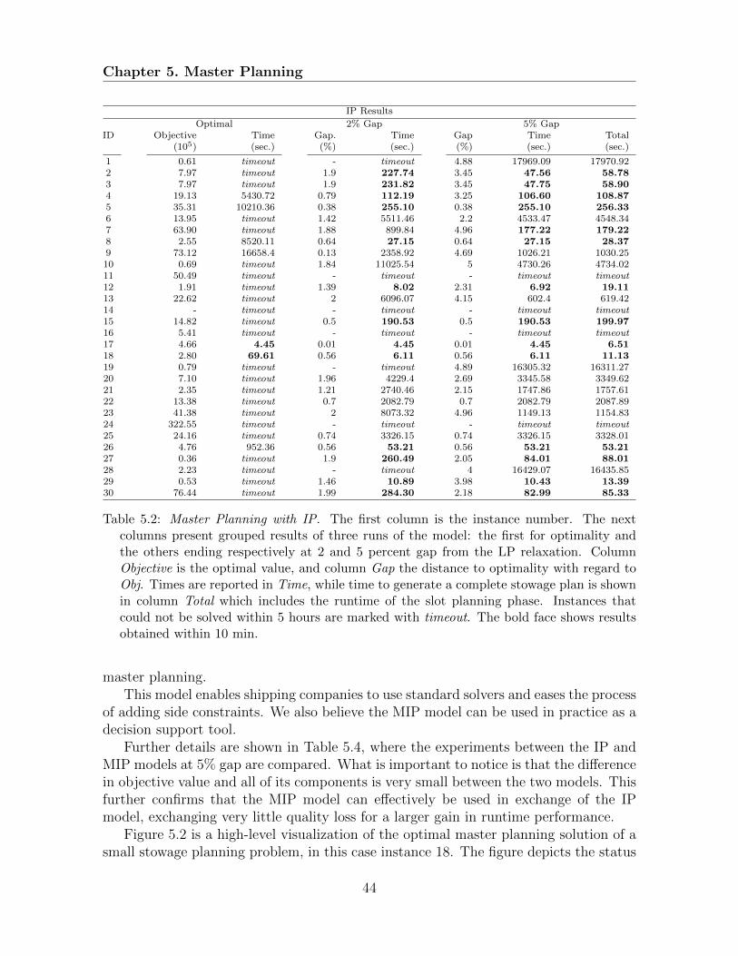
Chapter 5. Master Planning
IP Results
Optimal 2% Gap 5% GapID Objective Time Gap. Time Gap Time Total
(105) (sec.) (%) (sec.) (%) (sec.) (sec.)
1 0.61 timeout - timeout 4.88 17969.09 17970.922 7.97 timeout 1.9 227.74 3.45 47.56 58.783 7.97 timeout 1.9 231.82 3.45 47.75 58.904 19.13 5430.72 0.79 112.19 3.25 106.60 108.875 35.31 10210.36 0.38 255.10 0.38 255.10 256.336 13.95 timeout 1.42 5511.46 2.2 4533.47 4548.347 63.90 timeout 1.88 899.84 4.96 177.22 179.228 2.55 8520.11 0.64 27.15 0.64 27.15 28.379 73.12 16658.4 0.13 2358.92 4.69 1026.21 1030.2510 0.69 timeout 1.84 11025.54 5 4730.26 4734.0211 50.49 timeout - timeout - timeout timeout12 1.91 timeout 1.39 8.02 2.31 6.92 19.1113 22.62 timeout 2 6096.07 4.15 602.4 619.4214 - timeout - timeout - timeout timeout15 14.82 timeout 0.5 190.53 0.5 190.53 199.9716 5.41 timeout - timeout - timeout timeout17 4.66 4.45 0.01 4.45 0.01 4.45 6.5118 2.80 69.61 0.56 6.11 0.56 6.11 11.1319 0.79 timeout - timeout 4.89 16305.32 16311.2720 7.10 timeout 1.96 4229.4 2.69 3345.58 3349.6221 2.35 timeout 1.21 2740.46 2.15 1747.86 1757.6122 13.38 timeout 0.7 2082.79 0.7 2082.79 2087.8923 41.38 timeout 2 8073.32 4.96 1149.13 1154.8324 322.55 timeout - timeout - timeout timeout25 24.16 timeout 0.74 3326.15 0.74 3326.15 3328.0126 4.76 952.36 0.56 53.21 0.56 53.21 53.2127 0.36 timeout 1.9 260.49 2.05 84.01 88.0128 2.23 timeout - timeout 4 16429.07 16435.8529 0.53 timeout 1.46 10.89 3.98 10.43 13.3930 76.44 timeout 1.99 284.30 2.18 82.99 85.33
Table 5.2: Master Planning with IP. The first column is the instance number. The nextcolumns present grouped results of three runs of the model: the first for optimality andthe others ending respectively at 2 and 5 percent gap from the LP relaxation. ColumnObjective is the optimal value, and column Gap the distance to optimality with regard toObj. Times are reported in Time, while time to generate a complete stowage plan is shownin column Total which includes the runtime of the slot planning phase. Instances thatcould not be solved within 5 hours are marked with timeout. The bold face shows resultsobtained within 10 min.
master planning.This model enables shipping companies to use standard solvers and eases the process
of adding side constraints. We also believe the MIP model can be used in practice as adecision support tool.
Further details are shown in Table 5.4, where the experiments between the IP andMIP models at 5% gap are compared. What is important to notice is that the differencein objective value and all of its components is very small between the two models. Thisfurther confirms that the MIP model can effectively be used in exchange of the IPmodel, exchanging very little quality loss for a larger gain in runtime performance.
Figure 5.2 is a high-level visualization of the optimal master planning solution of asmall stowage planning problem, in this case instance 18. The figure depicts the status
44

Chapter 5. Master Planning
MIP Results
Optimal 2% Gap 5% GapID Gap Time Gap. Time Gap Time Total
(%) (sec.) (%) (sec.) (%) (sec.) (sec.)
1 - timeout - 1718.57 0.011 782.93 784.752 - 105.24 0.012 22.37 0.007 17.99 29.903 - 106.86 0.012 22.52 0.007 18.17 30.084 0.000 31.25 0.006 9.71 0.032 9.71 13.105 0.000 1074.08 0.003 47.65 0.003 47.65 48.796 - timeout 0.004 346.78 0.020 332.46 346.287 - timeout 0.008 143.74 0.008 92.19 94.958 0.002 16.91 0.006 5.68 0.006 5.68 7.359 0.000 107.01 0.001 101.28 0.049 101.28 106.5710 - 663.15 0.012 157.82 0.025 41.59 44.9511 - timeout - timeout - timeout timeout12 - 2.04 0.016 0.65 0.025 0.65 12.1713 - 17098.95 0.009 137.75 0.008 58.08 76.9214 - 645.51 - 13.09 - 13.09 13.0915 - 1304.77 0.012 16.05 0.012 16.05 24.8816 - 15844.06 - 8775.7 - 2665.65 2672.4817 0.001 1.77 0.006 1.54 0.006 1.54 4.0618 0.001 1.52 0.005 1.12 0.005 1.12 5.2919 - timeout - 216.28 0.009 81.55 87.3020 - 9050.47 0.010 70.43 0.017 70.43 74.3421 - timeout 0.006 84.36 0.027 72.88 82.9122 - timeout 0.011 61.80 0.021 12.14 20.4223 - timeout 0.005 1543.14 0.010 304.03 309.9724 - 2858.98 - 2328.33 - 1609.04 1615.8825 - timeout 0.004 63.63 0.013 37.92 39.6426 0.002 54.59 0.004 8.59 0.004 8.59 8.5927 - 93.86 0.000 4.95 0.013 4.40 6.5228 - timeout - 4624.16 0.017 1794.5 1799.8929 - 1.68 0.012 0.95 0.038 0.95 3.0630 - 102.41 0.002 37.54 0.024 28.02 30.85
Table 5.3: Master Planning with MIP. The second column describes the gap between the IPand MIP optimal solution. For the other columns see Table 5.2. Note that the gap in thistable is with regards to the corresponding IP solutions.
of the vessel upon arrival at each port. The top shows the state of the vessel as itarrives at the first port before any load or discharge operations are performed. The leftside depicts the load of each bay with a color coding indicating the port of discharge.On the right side, each of the vertical lines represents a transport assigned to a locationof the associated bay. The beginning of the line indicates the loading port and the endthe discharge port. The horizontal gray box between the vessels represents the ports.As illustrated, the crane makespan objective imposes a distribution of containers alongthe ship to maximize concurrent crane operations. Vessel bays, throughout the entireroute, also tend to hold most containers with the same port of discharge to minimizeoverstowage.
45
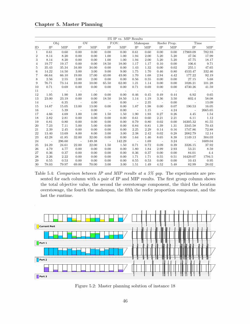
Chapter 5. Master Planning
5% IP vs. MIP Results
Obj OV P.OV. Makespan Reefer Prop. Time
ID IP MIP IP MIP IP MIP IP MIP IP MIP IP MIP
1 0.61 0.60 0.00 0.00 0.00 0.00 0.61 0.60 0.00 0.00 17969.09 782.932 8.14 8.20 0.00 0.00 1.00 1.00 1.94 2.00 5.20 5.20 47.56 17.993 8.14 8.20 0.00 0.00 1.00 1.00 1.94 2.00 5.20 5.20 47.75 18.174 19.77 19.17 0.00 0.00 18.50 18.00 1.17 1.17 0.10 0.00 106.6 9.715 35.43 35.34 34.00 34.00 0.00 0.00 1.43 1.32 0.00 0.02 255.1 47.656 14.22 14.50 3.00 3.00 9.00 9.00 1.75 1.70 0.46 0.80 4533.47 332.467 66.64 66.10 19.00 17.00 43.00 43.00 1.70 1.68 2.94 4.42 177.22 92.198 2.56 2.55 2.00 2.00 0.00 0.00 0.56 0.55 0.00 0.00 27.15 5.689 76.71 73.14 10.00 10.00 65.50 62.00 1.21 1.14 0.00 0.00 1026.21 101.2810 0.71 0.69 0.00 0.00 0.00 0.00 0.71 0.69 0.00 0.00 4730.26 41.5911 - - - - - - - - - - - -12 1.95 1.90 1.00 1.00 0.00 0.00 0.46 0.45 0.49 0.44 6.92 0.6513 23.00 23.19 0.00 0.00 18.50 18.50 1.14 1.19 3.36 3.50 602.4 58.0814 - 6.35 - 4.00 - 0.00 - 2.35 - 0.00 - 13.0915 14.87 15.05 13.00 13.00 0.00 0.00 1.87 1.98 0.00 0.07 190.53 16.0516 - 5.39 - 0.00 - 0.00 - 1.15 - 4.24 - 2665.6517 4.66 4.69 1.00 1.00 1.50 1.50 1.90 1.93 0.27 0.26 4.45 1.5418 2.82 2.81 0.00 0.00 0.00 0.00 0.61 0.60 2.21 2.21 6.11 1.1219 0.81 0.80 0.00 0.00 0.00 0.00 0.79 0.80 0.02 0.00 16305.32 81.5520 7.23 7.11 5.00 5.00 0.00 0.00 0.84 0.81 1.39 1.31 3345.58 70.4321 2.39 2.45 0.00 0.00 0.00 0.00 2.25 2.29 0.14 0.16 1747.86 72.8822 13.40 13.69 8.00 8.00 3.00 3.00 2.38 2.42 0.02 0.28 2082.79 12.1423 42.28 41.85 32.00 32.00 0.00 0.00 1.64 1.46 8.65 8.38 1149.13 304.0324 - 296.60 - 149.38 - 142.29 - 1.69 - 3.24 - 1609.0425 24.29 24.61 22.00 22.00 1.50 1.50 0.71 0.72 0.09 0.39 3326.15 37.9226 4.79 4.77 0.00 0.00 0.00 0.00 1.80 1.84 2.99 2.93 53.21 8.5927 0.36 0.37 0.00 0.00 0.00 0.00 0.36 0.37 0.00 0.00 84.01 4.428 2.26 2.22 0.00 0.00 0.00 0.00 1.71 1.71 0.55 0.51 16429.07 1794.529 0.55 0.53 0.00 0.00 0.00 0.00 0.55 0.53 0.00 0.00 10.43 0.9530 78.03 79.97 69.00 70.00 3.00 3.00 1.51 1.49 4.52 5.48 82.99 28.02
Table 5.4: Comparison between IP and MIP results at a 5% gap. The experiments are pre-sented for each column with a pair of IP and MIP results. The first group column showsthe total objective value, the second the overstowage component, the third the locationoverstowage, the fourth the makespan, the fifth the reefer proportion component, and thelast the runtime.
Figure 5.2: Master planning solution of instance 18
46
Chapter 5. Master Planning
5.4 An Improved Stability and Stress Model
Hydrostatic calculations, such as buoyancy, stability, trim and draft restrictions arenon-linear functions of the ship’s center of gravity and its displacement, (the totalweight of the loaded vessel). Those can, however, easily be linearized and translatedinto bounds on the position of the center of gravity when displacement is consideredconstant. This is the assumption in previous work and in the model presented in theprevious section.
In reality, ballast tanks are used by stowage coordinators to better handle the stabil-ity of the vessel and allow stowage configurations that are otherwise infeasible. Ignoringballast water can become a great source of error as it can constitute up to 25% of theship’s displacement. Including tanks in the mathematical models, however, brings fortha number of non-linear constraints due to the now variable vessel displacement.
When variable displacement is taken into account, the above mentioned hydrostaticcalculations becomes a function of two variables, the center of gravity and the displace-ment. The previously trivial linearization now becomes complex and difficult to handleefficiently. The intuition behind this complexity is simple. When the displacement isconstant, it is possible to pre-calculate the amount of water the vessel will displace.With variable displacement the amount of displaced water changes, and it does sonon-linearly due to the curved shape of the vessel hull.
According to our industrial collaborators, it is possible for stowage coordinators tomake an educated guess on the amount of ballast water that a vessel might need within15% of the actual amount. We use this assumption to define a displacement rangewithin which we are able to define a linearization of the stability constraints with anacceptable error.
5.4.1 Linearization of stability constraints
When ballast tanks are included into the optimization model there are two major non-linearities that need to be dealt with. The first is the calculation of the center of gravityand second is the linearization of the hydrostatic data. Consider the following equationfor the calculation of the longitudinal center of gravity (lcg) without ballast tanks:
LCG =LM o +
∑l∈LG
Ll vl
W(5.15)
where LM o is the constant longitudinal moment of the empty vessel, GLl is the longitu-
dinal center of gravity of location, l ∈ L, vl is the weight of location, l ∈ L and W is thedisplacement. Displacement is given by W = W o +
∑l∈L vl where W o is the constant
weight of the empty vessel. Since we load all the containers in the loadlist, the totalweight of the locations does not change and we can thus assume W to be constant,which makes equation (5.15) linear. Now let us consider the same equation where we
47
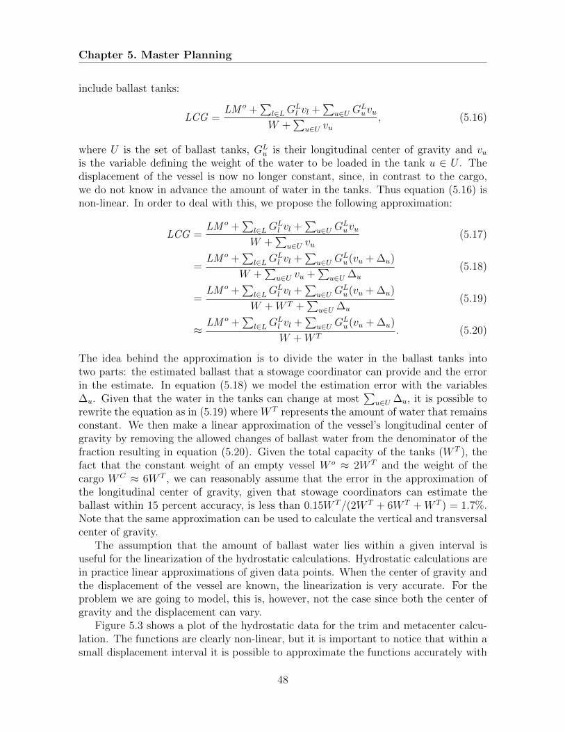
Chapter 5. Master Planning
include ballast tanks:
LCG =LM o +
∑l∈LG
Ll vl +
∑u∈U G
Luvu
W +∑
u∈U vu, (5.16)
where U is the set of ballast tanks, GLu is their longitudinal center of gravity and vu
is the variable defining the weight of the water to be loaded in the tank u ∈ U . Thedisplacement of the vessel is now no longer constant, since, in contrast to the cargo,we do not know in advance the amount of water in the tanks. Thus equation (5.16) isnon-linear. In order to deal with this, we propose the following approximation:
LCG =LM o +
∑l∈LG
Ll vl +
∑u∈U G
Luvu
W +∑
u∈U vu(5.17)
=LM o +
∑l∈LG
Ll vl +
∑u∈U G
Lu(vu + ∆u)
W +∑
u∈U vu +∑
u∈U ∆u
(5.18)
=LM o +
∑l∈LG
Ll vl +
∑u∈U G
Lu(vu + ∆u)
W +W T +∑
u∈U ∆u
(5.19)
≈LM o +
∑l∈LG
Ll vl +
∑u∈U G
Lu(vu + ∆u)
W +W T. (5.20)
The idea behind the approximation is to divide the water in the ballast tanks intotwo parts: the estimated ballast that a stowage coordinator can provide and the errorin the estimate. In equation (5.18) we model the estimation error with the variables∆u. Given that the water in the tanks can change at most
∑u∈U ∆u, it is possible to
rewrite the equation as in (5.19) where W T represents the amount of water that remainsconstant. We then make a linear approximation of the vessel’s longitudinal center ofgravity by removing the allowed changes of ballast water from the denominator of thefraction resulting in equation (5.20). Given the total capacity of the tanks (W T ), thefact that the constant weight of an empty vessel W o ≈ 2W T and the weight of thecargo WC ≈ 6W T , we can reasonably assume that the error in the approximation ofthe longitudinal center of gravity, given that stowage coordinators can estimate theballast within 15 percent accuracy, is less than 0.15W T/(2W T + 6W T + W T ) = 1.7%.Note that the same approximation can be used to calculate the vertical and transversalcenter of gravity.
The assumption that the amount of ballast water lies within a given interval isuseful for the linearization of the hydrostatic calculations. Hydrostatic calculations arein practice linear approximations of given data points. When the center of gravity andthe displacement of the vessel are known, the linearization is very accurate. For theproblem we are going to model, this is, however, not the case since both the center ofgravity and the displacement can vary.
Figure 5.3 shows a plot of the hydrostatic data for the trim and metacenter calcu-lation. The functions are clearly non-linear, but it is important to notice that within asmall displacement interval it is possible to approximate the functions accurately with
48
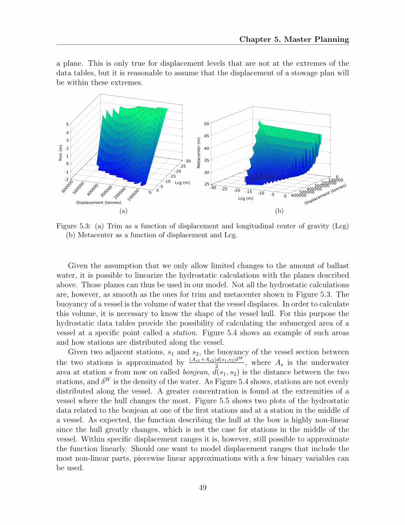
Chapter 5. Master Planning
a plane. This is only true for displacement levels that are not at the extremes of thedata tables, but it is reasonable to assume that the displacement of a stowage plan willbe within these extremes.
Trim
(m
)
Displacement (tonnes)
Lcg (m)
5
4
3
2
1
0
-1
-2
0-5
-10-15
-20-25
-30
0
1000
00
2000
00
3000
00
4000
00
5000
00
6000
00
(a)
Meta
cen
ter
(m)
Lcg (m)Disp
lacement (tonnes)25
30
35
40
45
50
-30 -25 -20 -15 -10 -5 0 600000500000
400000300000
200000100000
0
(b)
Figure 5.3: (a) Trim as a function of displacement and longitudinal center of gravity (Lcg)(b) Metacenter as a function of displacement and Lcg.
Given the assumption that we only allow limited changes to the amount of ballastwater, it is possible to linearize the hydrostatic calculations with the planes describedabove. Those planes can thus be used in our model. Not all the hydrostatic calculationsare, however, as smooth as the ones for trim and metacenter shown in Figure 5.3. Thebuoyancy of a vessel is the volume of water that the vessel displaces. In order to calculatethis volume, it is necessary to know the shape of the vessel hull. For this purpose thehydrostatic data tables provide the possibility of calculating the submerged area of avessel at a specific point called a station. Figure 5.4 shows an example of such areasand how stations are distributed along the vessel.
Given two adjacent stations, s1 and s2, the buoyancy of the vessel section between
the two stations is approximated by (As1+As2)d(s1,s2)δW
2, where As is the underwater
area at station s from now on called bonjean, d(s1, s2) is the distance between the twostations, and δW is the density of the water. As Figure 5.4 shows, stations are not evenlydistributed along the vessel. A greater concentration is found at the extremities of avessel where the hull changes the most. Figure 5.5 shows two plots of the hydrostaticdata related to the bonjean at one of the first stations and at a station in the middle ofa vessel. As expected, the function describing the hull at the bow is highly non-linearsince the hull greatly changes, which is not the case for stations in the middle of thevessel. Within specific displacement ranges it is, however, still possible to approximatethe function linearly. Should one want to model displacement ranges that include themost non-linear parts, piecewise linear approximations with a few binary variables canbe used.
49
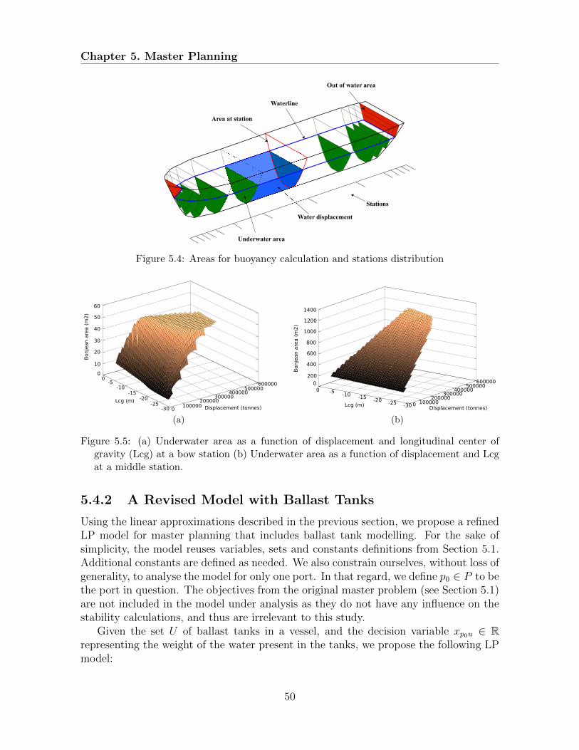
Chapter 5. Master Planning
Waterline
Out of water area
Area at station
Underwater area
Water displacement
Stations
Figure 5.4: Areas for buoyancy calculation and stations distribution
Bonje
an a
rea (
m2
)
Lcg (m)Displacement (tonnes)
60
50
40
30
20
10
00
-5-10
-15-20
-25-30
600000500000
400000300000
200000100000
0
(a)
Bon
jean
are
a (
m2
)
1400
1200
1000
800
600
400
200
00 -5
-10 -15 -20 -25 -30 0 100000200000
300000400000
500000600000
Lcg (m)Displacement (tonnes)
(b)
Figure 5.5: (a) Underwater area as a function of displacement and longitudinal center ofgravity (Lcg) at a bow station (b) Underwater area as a function of displacement and Lcgat a middle station.
5.4.2 A Revised Model with Ballast Tanks
Using the linear approximations described in the previous section, we propose a refinedLP model for master planning that includes ballast tank modelling. For the sake ofsimplicity, the model reuses variables, sets and constants definitions from Section 5.1.Additional constants are defined as needed. We also constrain ourselves, without loss ofgenerality, to analyse the model for only one port. In that regard, we define p0 ∈ P to bethe port in question. The objectives from the original master problem (see Section 5.1)are not included in the model under analysis as they do not have any influence on thestability calculations, and thus are irrelevant to this study.
Given the set U of ballast tanks in a vessel, and the decision variable xp0u ∈ Rrepresenting the weight of the water present in the tanks, we propose the following LPmodel:
50
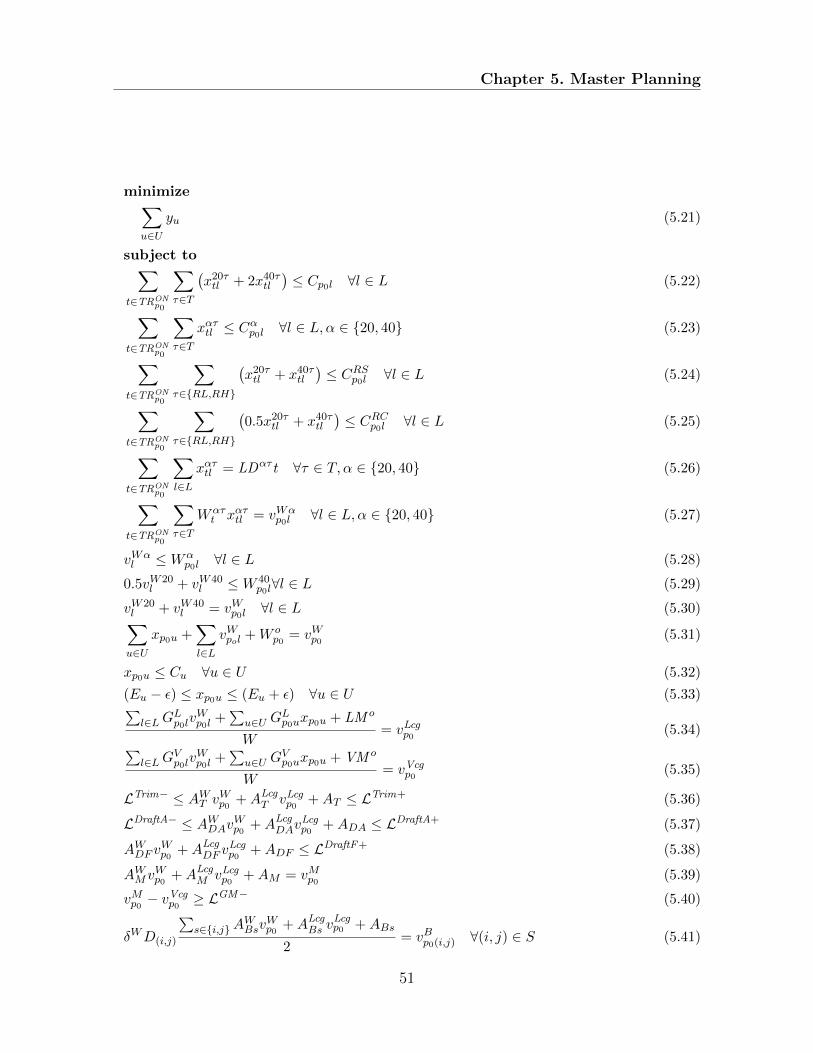
Chapter 5. Master Planning
minimize∑u∈U
yu (5.21)
subject to∑t∈TRON
p0
∑τ∈T
(x20τtl + 2x40τtl
)≤ Cp0l ∀l ∈ L (5.22)
∑t∈TRON
p0
∑τ∈T
xατtl ≤ Cαp0l ∀l ∈ L,α ∈ {20, 40} (5.23)
∑t∈TRON
p0
∑τ∈{RL,RH}
(x20τtl + x40τtl
)≤ CRSp0l ∀l ∈ L (5.24)
∑t∈TRON
p0
∑τ∈{RL,RH}
(0.5x20τtl + x40τtl
)≤ CRCp0l ∀l ∈ L (5.25)
∑t∈TRON
p0
∑l∈L
xατtl = LDατ t ∀τ ∈ T, α ∈ {20, 40} (5.26)
∑t∈TRON
p0
∑τ∈T
Wατt xατtl = vWα
p0l ∀l ∈ L,α ∈ {20, 40} (5.27)
vWαl ≤Wα
p0l ∀l ∈ L (5.28)
0.5vW20l + vW40
l ≤W 40p0l∀l ∈ L (5.29)
vW20l + vW40
l = vWp0l ∀l ∈ L (5.30)∑u∈U
xp0u +∑l∈L
vWpol +W op0 = vWp0 (5.31)
xp0u ≤ Cu ∀u ∈ U (5.32)
(Eu − ε) ≤ xp0u ≤ (Eu + ε) ∀u ∈ U (5.33)∑l∈LG
Lp0lvWp0l +
∑u∈U G
Lp0uxp0u + LM o
W= vLcgp0 (5.34)∑
l∈LGVp0lvWp0l +
∑u∈U G
Vp0uxp0u + VM o
W= vVcg
p0 (5.35)
LTrim− ≤ AWT vWp0 +ALcgT vLcgp0 +AT ≤ LTrim+ (5.36)
LDraftA− ≤ AWDAvWp0 +ALcgDAv
Lcgp0 +ADA ≤ LDraftA+ (5.37)
AWDF vWp0 +ALcg
DF vLcgp0 +ADF ≤ LDraftF+ (5.38)
AWMvWp0 +ALcg
M vLcgp0 +AM = vMp0 (5.39)
vMp0 − vVcgp0 ≥ L
GM− (5.40)
δWD(i,j)
∑s∈{i,j}A
WBsv
Wp0 +ALcg
Bs vLcgp0 +ABs
2= vBp0(i,j) ∀(i, j) ∈ S (5.41)
51

Chapter 5. Master Planning
Wαf +
∑l∈L
pαlfvWp0l +
∑u∈U
pαufxp0u −∑s∈S
pαsfvBp0f = vSαp0f ∀f ∈ F, α ∈ {Aft ,Fore} (5.42)
Mαf +∑l∈L
aαlfpαlfv
Wp0l +
∑u∈U
aαufpαufxp0u−
∑s∈S
aαsfpαsfv
Bp0s = vBαp0f ∀f ∈ F, α ∈ {Aft ,Fore} (5.43)
LShear−p0f≤ wfvsForep0f + (1− wf )vSAft
p0f≤ LShear+p0f
(5.44)
LBending−p0f
≤ wfvBForep0f + (1− wf )vBAft
p0f≤ LBending+
p0f(5.45)
Eu − xu ≤ yu ∀u ∈ U (5.46)
xu − Eu ≤ yu ∀u ∈ U (5.47)
Constraints (5.22), (5.23), (5.24) and (5.26) are equivalent to constraints (5.2), (5.4),(5.3) and (5.5) of the previous model, and are therefore not further discussed.
Once a 20’ container is placed on a reefer cell, if that cell has two reefer plugs,the cell-wise capacity is reduced as the extra plug cannot be used for a 40’ container.For that reason an extra constraint for the reefer cell’s capacity (CRC
p0l) is required,
(constraint (5.25)). Chapter 2 discussed how the weight of 20’ and 40’ containers dif-ferently affect the structure of the vessel. To achieve a more accurate model, we takethis information into account with constraint (5.27) that defines the variables vW20
p0land
vW40p0l
, holding the weight of the 20’ and 40’ containers in location l ∈ L respectively.With constraint (5.28) we constrain each of the variables to the respective limits W 20
p0l
and W 40p0l
. The combined total weight is constrained in (5.29). All stability calcula-tions are based on the weight of containers in a location. Constraint (5.30) definesthe auxiliary variable vWp0l representing the weight of containers in location l ∈ L. Thedisplacement (total weight), of the vessel is represented by the auxiliary variable vWp0with constraint (5.31) where W o
p0is the constant weight of the empty vessel and on-
board containers. Constraint (5.32) defines the capacity (Cu) of the tanks, while givenEu as the initial condition of the tanks, constraint (5.33) defines the allowed ε ballastchange. Variable vLcgp0l
represents the longitudinal center of gravity of location l and iscomputed in constraint (5.34) using the approximation defined in (5.20). The constantLM o is the constant longitudinal moment of the vessel, GL
p0uis the longitudinal center
of gravity of the tank u ∈ U and W is the approximated constant displacement. Thesame approximation is used in constraint (5.35) for the calculation of the vertical centerof gravity represented by the variable vVcg
p0. Given the displacement of the vessel vWp0
and its approximated longitudinal center of gravity vLcgp0, constraint (5.36) approximates
trim with a plane given by the coefficients AWT , ALcgT and AT . The calculated trim is then
required to be within the limits LTrim− and LTrim+. Changing the coefficients accord-ingly, constraint (5.37) and (5.38) approximate the aft and fore draft of the vessel. Bothdrafts are kept within the maximum limits LDraftA+ and LDraftF+. Due to the propellerit is also necessary to constrain the draft aft to be at least LDraftA−. The metacenter isalso calculated using a linear approximation and is defined in constraint (5.39) by thevariable vMp0 . The GM is then calculated in constraint (5.40) and required to be abovethe limit LGM . The buoyancy of the section of a vessel between two adjacent stations
52

Chapter 5. Master Planning
is defined in constraint (5.41) by the variable vBpo(i,j). Set S is the set of adjacent station
pairs (i, j), D(ij) is the distance between the two stations, and δW is the density ofthe water. Again, the hydrostatic linearization is used in this calculation. In shear andbending calculations we take into account the forces at play aft or fore of a frame. Sinceframes do not always coincide with the starting points of tanks, locations or buoyancystations, it is necessary to know, given a frame f ∈ F , the fraction of weight thatneeds to be taken into account from a location l, tank u or station s. For this purposethe constant pAft
lf ∈ [0, 1] is used to denote the fraction of cargo to be considered from
location l ∈ L aft of frame f ∈ F and pForelf for the fraction fore of the frame (pAftuf , p
Foreuf
for the tanks and pAftsf , p
Foresf for the buoyancy). Since the shear forces and bending mo-
ments are calculated per frame, errors in the linearization accumulate the further awayfrom the calculation frame the weights are. This can become problematic in the caseof bending where the forces are multiplied by the arm, thereby substantially increasingthe approximation error. Shear and bending calculations can be done for either thefore or aft part of a frame. It stands to reason that aft stress calculations are moreaccurate at the stern of the vessel and fore calculations at the bow. For that reason amore precise modelling of stress forces requires the calculation at both the aft and forepart of a frame where the two resulting stresses are blended such that aft calculationsare weighted more at stern and less at bow. Constraint (5.42) calculates the shearforces both aft and fore of each frame f ∈ F and defines the shear variable vSp0f , andwhere Wαf is the constant weight aft or fore of frame f . The final shear calculationwhere the aft and fore shear are mixed using a scaling factor wf ∈ [0, 1] (such thatit is 1 for the first frame at bow and 0 in the first frame at stern), is kept within thelimits LShear+
p0fand LShear−
p0fin constraint (5.44). The same calculation is made for the
bending. The bending variable vBαp0f is defined in constraint (5.43) where aαlf , aαuf , a
αsf
are the arm to frame f ∈ F of location l ∈ L, tank u ∈ U and buoyancy sections ∈ S for both the aft and fore calculation. The constant moment of the vessel is givenby the constant M o
f and bending is kept within the limits LBending+p0f
and LBending−p0f
byconstraint (5.45). Constraints (5.46) and (5.47) define the cost variable yu quantifyingthe changes in tank configuration from the initial estimate. The approximation errorincreases with the amount of difference from the estimated amount of water in eachtank, thus objective 5.21 minimizes this difference.
5.4.3 Analysis of Model Accuracy
The improved model for stability and stress calculations, was evaluated experimentallyon a large container vessel with a capacity of about 15,000 TEUs. This vessel was usedas a case study where a set of 10 stowage plans were analysed. The stowage planswere taken directly from actual historical data and are thus representative of the loadsthat can be expected on such vessels at any given port. Table 5.5 gives an overview ofthe test instance characteristics. In order to evaluate the solutions, we compare witha manual calculation. The manual calculation uses the actual displacement and center
53
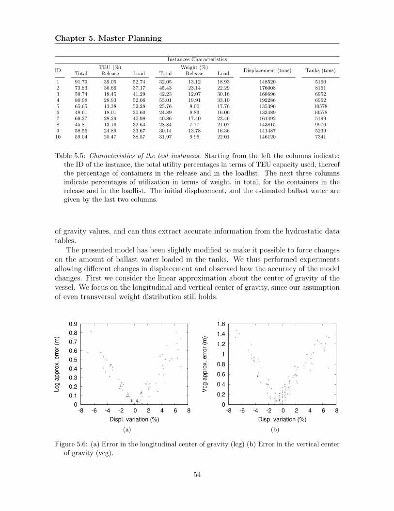
Chapter 5. Master Planning
Instances Characteristics
IDTEU (%) Weight (%)
Displacement (tons) Tanks (tons)Total Release Load Total Release Load
1 91.79 39.05 52.74 32.05 13.12 18.93 148520 51602 73.83 36.66 37.17 45.43 23.14 22.29 176008 81613 59.74 18.45 41.29 42.23 12.07 30.16 168696 69524 80.98 28.93 52.06 53.01 19.91 33.10 192286 69625 65.65 13.38 52.28 25.76 8.00 17.76 135396 105786 48.61 18.01 30.60 24.89 8.83 16.06 133489 105787 69.27 28.29 40.98 40.86 17.40 23.46 161492 51998 45.81 13.16 32.64 28.84 7.77 21.07 143815 99769 58.56 24.89 33.67 30.14 13.78 16.36 141487 523910 59.04 20.47 38.57 31.97 9.96 22.01 146120 7341
Table 5.5: Characteristics of the test instances. Starting from the left the columns indicate:the ID of the instance, the total utility percentages in terms of TEU capacity used, thereofthe percentage of containers in the release and in the loadlist. The next three columnsindicate percentages of utilization in terms of weight, in total, for the containers in therelease and in the loadlist. The initial displacement, and the estimated ballast water aregiven by the last two columns.
of gravity values, and can thus extract accurate information from the hydrostatic datatables.
The presented model has been slightly modified to make it possible to force changeson the amount of ballast water loaded in the tanks. We thus performed experimentsallowing different changes in displacement and observed how the accuracy of the modelchanges. First we consider the linear approximation about the center of gravity of thevessel. We focus on the longitudinal and vertical center of gravity, since our assumptionof even transversal weight distribution still holds.
0
0.1
0.2
0.3
0.4
0.5
0.6
0.7
0.8
0.9
-8 -6 -4 -2 0 2 4 6 8
Lcg a
ppro
x. err
or
(m)
Displ. variation (%)
(a)
0
0.2
0.4
0.6
0.8
1
1.2
1.4
1.6
-8 -6 -4 -2 0 2 4 6 8
Vcg a
ppro
x. err
or
(m)
Disp. variation (%)
(b)
Figure 5.6: (a) Error in the longitudinal center of gravity (lcg) (b) Error in the vertical centerof gravity (vcg).
54
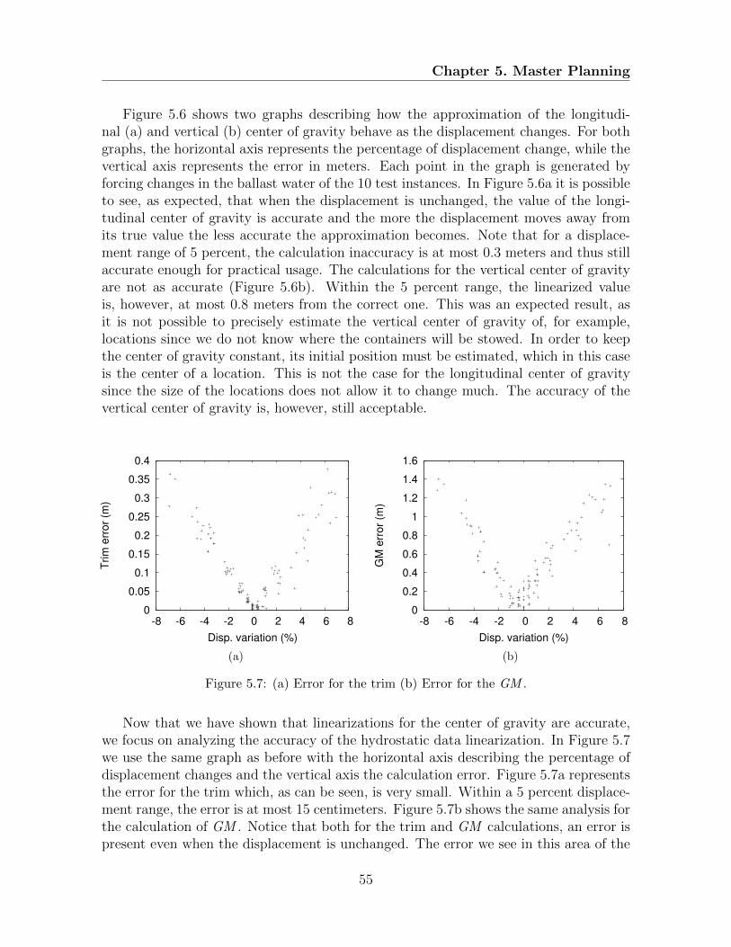
Chapter 5. Master Planning
Figure 5.6 shows two graphs describing how the approximation of the longitudi-nal (a) and vertical (b) center of gravity behave as the displacement changes. For bothgraphs, the horizontal axis represents the percentage of displacement change, while thevertical axis represents the error in meters. Each point in the graph is generated byforcing changes in the ballast water of the 10 test instances. In Figure 5.6a it is possibleto see, as expected, that when the displacement is unchanged, the value of the longi-tudinal center of gravity is accurate and the more the displacement moves away fromits true value the less accurate the approximation becomes. Note that for a displace-ment range of 5 percent, the calculation inaccuracy is at most 0.3 meters and thus stillaccurate enough for practical usage. The calculations for the vertical center of gravityare not as accurate (Figure 5.6b). Within the 5 percent range, the linearized valueis, however, at most 0.8 meters from the correct one. This was an expected result, asit is not possible to precisely estimate the vertical center of gravity of, for example,locations since we do not know where the containers will be stowed. In order to keepthe center of gravity constant, its initial position must be estimated, which in this caseis the center of a location. This is not the case for the longitudinal center of gravitysince the size of the locations does not allow it to change much. The accuracy of thevertical center of gravity is, however, still acceptable.
0
0.05
0.1
0.15
0.2
0.25
0.3
0.35
0.4
-8 -6 -4 -2 0 2 4 6 8
Trim
err
or
(m)
Disp. variation (%)
(a)
0
0.2
0.4
0.6
0.8
1
1.2
1.4
1.6
-8 -6 -4 -2 0 2 4 6 8
GM
err
or
(m)
Disp. variation (%)
(b)
Figure 5.7: (a) Error for the trim (b) Error for the GM .
Now that we have shown that linearizations for the center of gravity are accurate,we focus on analyzing the accuracy of the hydrostatic data linearization. In Figure 5.7we use the same graph as before with the horizontal axis describing the percentage ofdisplacement changes and the vertical axis the calculation error. Figure 5.7a representsthe error for the trim which, as can be seen, is very small. Within a 5 percent displace-ment range, the error is at most 15 centimeters. Figure 5.7b shows the same analysis forthe calculation of GM . Notice that both for the trim and GM calculations, an error ispresent even when the displacement is unchanged. The error we see in this area of the
55
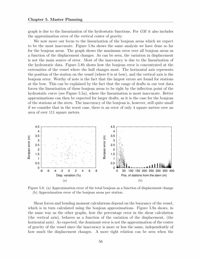
Chapter 5. Master Planning
graph is due to the linearization of the hydrostatic functions. For GM it also includesthe approximation error of the vertical center of gravity.
We now move our focus to the linearization of the bonjean areas which we expectto be the most inaccurate. Figure 5.8a shows the same analysis we have done so farfor the bonjean areas. The graph shows the maximum error over all bonjean areas asa function of the displacement changes. As can be seen, the variation in displacementis not the main source of error. Most of the inaccuracy is due to the linearization ofthe hydrostatic data. Figure 5.8b shows how the bonjean error is concentrated at theextremities of the vessel where the hull changes most. The horizontal axis representsthe position of the station on the vessel (where 0 is at bow), and the vertical axis is thebonjean error. Worthy of note is the fact that the largest errors are found for stationsat the bow. This can be explained by the fact that the range of drafts in our test dataforces the linearization of these bonjean areas to be right by the inflection point of thehydrostatic curve (see Figure 5.5a), where the linearization is most inaccurate. Betterapproximations can then be expected for larger drafts, as it is the case for the bonjeanof the stations at the stern. The inaccuracy of the bonjean is, however, still quite smallif we consider that in the worst case, there is an error of only 4 square meters over anarea of over 111 square meters.
0
0.5
1
1.5
2
2.5
3
3.5
4
4.5
-8 -6 -4 -2 0 2 4 6 8
Bonje
an e
rror
(m)
Disp. variation (%)
(a)
0
0.5
1
1.5
2
2.5
3
3.5
4
4.5
0 50 100 150 200 250 300 350 400
Bonje
an e
rror
(m)
Pos. of stations from the stern (m)
(b)
Figure 5.8: (a) Approximation error of the total bonjean as a function of displacement change(b) Approximation error of the bonjean areas per station.
Shear forces and bending moment calculations depend on the buoyancy of the vessel,which is in turn calculated using the bonjean approximations. Figure 5.9a shows, inthe same way as the other graphs, how the percentage error in the shear calculation(the vertical axis), behaves as a function of the variation of the displacement, (thehorizontal axis). As expected, the dominant error is not the approximation of the centerof gravity of the vessel since the inaccuracy is more or less the same, independently ofhow much the displacement changes. A more tight relation can be seen when the
56

Chapter 5. Master Planning
shear calculation is related to the error in the bonjean linearization. Figure 5.9b showsthe percentage error of the shear force calculation as a function of the total error inbonjean area from the hydrostatic linearization. As depicted, the error in the shearcalculation increases with the error in the bonjean linearization. The graph also groupsthe data points according to their displacement range, and for the data points with nodisplacement change we can see that the tendency remains the same. One must alsotake into account that the linearization error of the bonjean is amplified in the shearforces calculation by the fact that it becomes accumulated in the summation of theforces. This particular information is very important when analyzing the error in thebending moment calculation, since this accumulated error is multiplied by the arm ofthe moment and thus multiplies its impact.
0
0.2
0.4
0.6
0.8
1
1.2
1.4
-8 -6 -4 -2 0 2 4 6 8
Shear
forc
e e
rror
(%)
Disp. variation (%)
(a)
0
0.2
0.4
0.6
0.8
1
1.2
1.4
2 4 6 8 10 12 14 16 18 20
Shear
forc
e e
rror
(%)
Total bonjean error (m2)
[-10,-5][-5,-2.5][-2.5,-1][-1,-0.1]
[-0.1,0.1]
[0.1,1][1,2.5]
[2.5, 5][5,10]
(b)
Figure 5.9: (a) Approximation error of the shear forces as a function of displacement change(b) Approximation error of the shear forces as a function of the total bonjean error.
Figure 5.10a shows the error in the bending calculation as a function of the changesin displacement. As expected, comparable to the shear force calculation, the mainsource of error is not the approximation of the longitudinal center of gravity, but ratherthe error in the linearization of the bonjean areas. Due to the fact that the bonjeanerror is amplified by the multiplication of the arm, it is necessary to look at the errorat each calculation frame in order to see how the error of the bending moment changes.We do this by forcing the displacement to remain constant, thus removing the error ofthe longitudinal center of gravity approximation, and analyzing how the bending errorchanges at each calculation frame as the draft of each of the 10 test instances changes.The result is shown in Figure 5.10b, where the horizontal axis represents the framesof the vessel and the vertical axis is the percentage of error in the bending momentcalculation. Each of the lines plotted in the graph represent one of the 10 test instanceseach of which has a different draft. As expected, the bending moment is less accurateat the bow and stern due to the imprecision in the bonjean calculations. One more
57

Chapter 5. Master Planning
0
1
2
3
4
5
6
-8 -6 -4 -2 0 2 4 6 8
Bendin
g a
ppro
x. err
or
(%)
Disp. variation (%)
(a)
0
0.2
0.4
0.6
0.8
1
1.2
1.4
0 5 10 15 20 25
Bendin
g a
ppro
x. err
or
(%)
Frames from the AP
Draft 10.76Draft 11.43Draft 11.52Draft 11.72Draft 12.53Draft 14.38
(b)
Figure 5.10: (a) Approximation error of the bending moment as a function of displacementchange (b) Approximation error of the bending moment at each bonjean station.
thing worthy of notice is that there is no direct relation between the bending error andthe draft of the vessel. This is due to the non-linear shape of the hull. The bendingerror for constant displacement does not exceed 1.4 percent. However, when variabledisplacement is considered an error of up to 3.5 percent might be reached within a 5percent displacement variation. We consider these approximations acceptable. Higheraccuracy can be achieved by reducing the linearization error of the hydrostatic functionsfor bonjean.
58

Chapter 6. Slot Planning
Chapter 6
Slot Planning
The slot planning phase refines the plan generated during master planning. It assignsthe containers associated with each location to specific slots within the location. Itis during this phase that container stacking constraints are handled. The abstracteddecisions taken during master planning might, however, not always be feasible. Slotplanning must thus be able to handle these situations. The master planning objectives,minimization of overstowage and minimization of crane makespan, produce master planswhere the average number of discharge ports per location is close to one. This becomes afeature of the input of the slot planning instances. In comparison to the general problemcomplexity, the instances are thus much simpler, as far as overstowage is concerned.We therefore expect heuristic solutions to achieve high quality solutions fast.
As previously mentioned (chapter 5), such efficiency in runtime allows us to spendmost of the time in the harder master planning phase. The slot planning phase usesthe following simple algorithm:
1. The container to slot assignment for a specific location is solved using the con-straint programming model of Delgado et al. (2012).
2. If no solution is found within a given time limit, the problem is solved using aCBLS algorithm.
3. If no feasible solution is found, a heuristic procedure drops containers until afeasible solution is found.
(a) The feasible solution is optimized using the same CBLS algorithm.
The CBLS algorithm and the procedure to handle infeasible instances are part of theresearch behind this thesis and are described in detail in the following sections.
6.1 The Slot Planning Problem
The slot planing problem solved in this thesis includes both 20’ and 40’ containers. Asan example of containers with special requirements, it considers reefer and high-cube
59
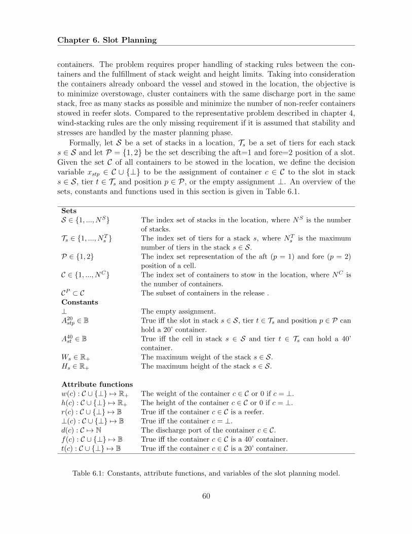
Chapter 6. Slot Planning
containers. The problem requires proper handling of stacking rules between the con-tainers and the fulfillment of stack weight and height limits. Taking into considerationthe containers already onboard the vessel and stowed in the location, the objective isto minimize overstowage, cluster containers with the same discharge port in the samestack, free as many stacks as possible and minimize the number of non-reefer containersstowed in reefer slots. Compared to the representative problem described in chapter 4,wind-stacking rules are the only missing requirement if it is assumed that stability andstresses are handled by the master planning phase.
Formally, let S be a set of stacks in a location, Ts be a set of tiers for each stacks ∈ S and let P = {1, 2} be the set describing the aft=1 and fore=2 position of a slot.Given the set C of all containers to be stowed in the location, we define the decisionvariable xstp ∈ C ∪ {⊥} to be the assignment of container c ∈ C to the slot in stacks ∈ S, tier t ∈ Ts and position p ∈ P , or the empty assignment ⊥. An overview of thesets, constants and functions used in this section is given in Table 6.1.
SetsS ∈ {1, ..., NS} The index set of stacks in the location, where NS is the number
of stacks.Ts ∈ {1, ..., NT
s } The index set of tiers for a stack s, where NTs is the maximum
number of tiers in the stack s ∈ S.P ∈ {1, 2} The index set representation of the aft (p = 1) and fore (p = 2)
position of a cell.C ∈ {1, ..., NC} The index set of containers to stow in the location, where NC is
the number of containers.CP ⊂ C The subset of containers in the release .Constants⊥ The empty assignment.A20stp ∈ B True iff the slot in stack s ∈ S, tier t ∈ Ts and position p ∈ P can
hold a 20’ container.A40st ∈ B True iff the cell in stack s ∈ S and tier t ∈ Ts can hold a 40’
container.Ws ∈ R+ The maximum weight of the stack s ∈ S.Hs ∈ R+ The maximum height of the stack s ∈ S.
Attribute functionsw(c) : C ∪ {⊥} 7→ R+ The weight of the container c ∈ C or 0 if c = ⊥.h(c) : C ∪ {⊥} 7→ R+ The height of the container c ∈ C or 0 if c = ⊥.r(c) : C ∪ {⊥} 7→ B True iff the container c ∈ C is a reefer.⊥(c) : C ∪ {⊥} 7→ B True iff the container c = ⊥.d(c) : C 7→ N The discharge port of the container c ∈ C.f(c) : C ∪ {⊥} 7→ B True iff the container c ∈ C is a 40’ container.t(c) : C ∪ {⊥} 7→ B True iff the container c ∈ C is a 20’ container.
Table 6.1: Constants, attribute functions, and variables of the slot planning model.
60
Chapter 6. Slot Planning
We propose a logic based model. A feasible solution to the proposed slot planningproblem fulfills the following constraints:
∀s ∈ S, t ∈ Ts .¬f(xst1) ∧ (f(xst2)⇒ ⊥(xst1)) (6.1)
∀s ∈ S, t ∈ Ts \ {1}, p ∈ P .¬⊥(xstp)⇒(t(xs(t−1)1) ∧ t(xs(t−1)2)
)∨ f(xs(t−1)1) (6.2)
∀s ∈ S, t ∈ Ts, p ∈ P . t(xstp)⇒ A20stp (6.3)
∀s ∈ S, t ∈ Ts . f(xst1)⇒ A40st (6.4)
∀s ∈ S, t ∈ Ts \ {NTs }, p ∈ P . f(xst1)⇒ ¬t(xs(t+1)p) (6.5)
∀c ∈ C . |{xstp = c | s ∈ S, t ∈ Ts, p ∈ P}| = 1 (6.6)
∀c ∈ CP . xsctcpc = c (6.7)
∀s ∈ S, t ∈ Ts, p ∈ P . r(xstp) ∧ t(xstp)⇒ ARstp (6.8)
∀s ∈ S, t ∈ Ts . r(xst1) ∧ f(xst1)⇒ ARst1 ∨ ARst2 (6.9)
∀s ∈ S .∑t∈Ts
(w(xst1) + w(xst2)) ≤ Ws (6.10)
∀s ∈ S .∑t∈Ts
max(h(xst1), h(xst2)) ≤ Hs (6.11)
The assignment convention for the 40’ containers is maintained by constraint (6.1),where f(c) indicates if container c ∈ C ∪ {⊥} is a 40’ container and ⊥(c) indicates itis an empty assignment (c = ⊥). Physical support from below is guaranteed for allcontainers via constrains (6.2), where t(c) is true if container c ∈ C ∪ {⊥} is a 20’container. Cell capacities for 20’ and 40’ containers are fulfilled by constraint (6.3) and(6.4), where the constant A20
stp is the 20’ capacity of a slot and A40st is the 40’ capacity of
a cell. Stacking rules between 20’ and 40’ containers are modelled by constraint (6.5),where NT
s is the index of the top tier in stack s ∈ S. Each container is assigned toexactly one slot (6.6). Given a set of release containers CP constraint (6.7), ensures theoriginal assignment (sc, tc, pc), is maintained.
Reefer slots are indicated with the constant ARstp = true, and 20’ reefer containersare forced to be stowed in those slots by constraint (6.8), while (6.9), ensures that 40’reefer containers are stowed in cells where either one of the two slots has a power-plug.Reefer containers are identified by the function r(c). Stacks weights and heights aremaintained within limits by constraints (6.10) and (6.11), where w(c) and h(c) arerespectively the weight and height of container c ∈ C ∪ {⊥}. Stack weight and heightlimits are defined by the constants Ws and Hs
Two of the objectives modelled in the slot planning phase are known from theliterature, namely overstowage minimization and the clustering of containers with thesame discharge port on one stack. The other objectives have not been modelled beforeand are aimed to generating a robust plan. The first of these attempts at leaving asmany stacks free of containers as possible, thus generating space in the location for thenext ports. The second, reduces the number of non-reefer containers stowed in reefer
61

Chapter 6. Slot Planning
slots since those are scarce. Following is the modelling of the slot planning objectivecomponents:
oos =∑s∈S
∑t∈Ts
∑p∈P
ostp (6.12)
our =∑s∈S
∑t∈Ts
∑p∈P
urstp (6.13)
ops =∑s∈S
| {d(xstp) | t ∈ Ts, p ∈ P ,¬⊥(xstp)} | (6.14)
ous =∑s∈S
uss (6.15)
In (6.12) one unit of cost is counted for each container that is overstowing anotherone below in the stack, where ostp defines whether a container c ∈ C in stack s ∈ S,tier t ∈ Ts and slot position p ∈ P overstows another container in the stack. Thus,ostp = 1 if ¬⊥(xstp) and there exists a tier t′ ∈ {ts, ..., t− 1} below t with an overstowedcontainer d(xst′p) < d(xstp) (d(c) return the discharge port of container c). Otherwiseostp = 0. Objective (6.13), counts one unit cost for each misused reefer slot, whereurstp = 1 if ARstp and (f(xst1) ∧ ¬r(xst1) ∨ t(xstp) ∧ ¬r(xstp)), and 0 otherwise. Noticethat a 40’ non-reefer container will add a unit cost for each reefer slot it covers. In orderto favor stacks stowing containers with the same port of destination, one unit cost iscounted for each discharge port present in the stack, (6.14). In order to minimize thenumber of used stacks, one unit cost for each stack used is counted by (6.15), whereuss = 1 if there exists a t ∈ Ts and p ∈ P such that ¬⊥(xstp), and 0 otherwise.
An optimal solution to a slot planning problem optimizes the following weightedsum:
min COoos + CCops + CSous + CRour (6.16)
where the cost weights CO, CC , CS and CR represent the priority given to each objectiveby the stowage coordinators.
6.2 Constraint-Based Local Search (CBLS)
CBLS is an architecture for combinatorial local search algorithms based on the conceptof constraints and objectives. The constraint satisfaction part of a combinatorial opti-mization problem is transformed into an optimization problem where the objective isto minimize constraint violations.
At the core of the architecture we find the concept of invariants or one-way con-straints. Invariants are represented by incremental variables which express a relation-ship that must be maintained once a new assignment is made to the decision variables.Consider the following example:
v =n∑i=1
xi (6.17)
62

Chapter 6. Slot Planning
where xi is a decision variable and v is an incremental variable. Expression (6.17) is aninvariant, and each time a variable xi assumes a new value, the incremental variable vmust be updated accordingly.
Once invariants are available it is natural to create compound objects that maintainproperties incrementally. Those objects are called differentiable objects. An example ofthose are constraints and objectives. Differentiable objects maintain properties such assatisfiability, violations and the contribution of each variable to the violation. Complexfunctions and evaluations to differentiate similar solutions can also be maintained.
In order to incrementally maintain the system, it is enough to implement an in-cremental algorithm for the basic invariants based on the neighborhood operator ofchoice.
It is now possible to define formal models of combinatorial problems that make use ofthe invariant and differentiable objects. Such a model then provides the means to definesearch algorithms that use the available information, such as constraint violations, forheuristic decisions. This way it is effectively possible to divide the modelling and searchparts of local search algorithms.
We refer the reader to Hentenryck and Michel (2009) for an in-depth description ofthe architecture and the concepts behind CBLS.
6.3 A CBLS for Slot Planning
The CBLS algorithm proposed for slot planning is a classical hill-climbing search usingthe min-conflict heuristic (Minton et al., 1992). The initial solution is given by a place-ment heuristic that relaxes the weight and height constraints to find an initial containerarrangement which minimises the objective function. After the initial configuration isfound, the algorithm diverges from its classical definition by first focusing on findinga feasible solution with respect to the constraints. Once such a solution is found, itis possible to constrain the neighborhood function to remain within the feasible regionwhile optimizing the objectives.
The aim is to gradually reduce the complexity of the problem in such a way that afeasible solution is found fast, allowing the algorithm to use more time searching for anoptimal solution. In order for the algorithms to pursue different search paths, random-ization is used whenever possible and a race between parallel searches is performed.
The CBLS algorithm uses a neighborhood generated by swapping containers withinthe location. A swap is an exchange of some containers between a pair of cells. Formally,a swap γ is a pair of tuples γ = (〈s, t, c〉, 〈s′, t′, c′〉) where the containers c in the cellin stack s and tier t exchange position with the containers c′ in the cell in stack s′ andtier t′. The sets c and c′ can contain at most two containers. Swaps are implementedwith two functions swap20 for exchanging position of 20’ containers, and swap40 forexchanging position of 40’ containers.
• swap20(xstp, xs′t′p′) where p 6= p′ if (s, t) = (s′, t′), swaps the value of xstp and xs′t′p′and covers the following swap types 1) 20′ ↔ 20′ and 2) ⊥ ↔ 20′.
63
Chapter 6. Slot Planning
• swap40 ((xst1, xst2), (xs′t′1, xs′t′2)) where (s, t) 6= (s′, t′), pairwise swaps the valuesof the cell variables (xst1, xst2) and (xs′t′1, xs′t′2) and covers the following swaptypes 1) (40′,⊥) ↔ (40′,⊥), 2) (⊥, 20′) ↔ (40′,⊥), 3) (20′,⊥) ↔ (40′,⊥), 4)(20′, 20′)↔ (40′,⊥) and, 5) (⊥,⊥)↔ (40′,⊥).
Proposition 2. The swap neighborhood Γ defined by the union of swap20 and swap40
swaps for a slot planning problem Π is complete.
Proof in Appendix C.
6.3.1 Constraint Violations
In CBLS it is common to evaluate and represent a constraint in terms of the set ofvariables that violate it. When the violation of a constraint is 0 the constraint issatisfied. When a variable violates a constraint, its violation degree is either fixed, (e.g,1) or it reflects to which extent the variable breaks the constraint. This representationis ideal when using the min-conflict heuristic, since it makes it possible to identify whichvariable violates most constraints and to what degree.
Let πstp denote the value of variable xstp in assignment π. Each constraint andobjective is then defined in terms of a function σ(π) on the assignment π of variablesover the violations of each slot variable defined by ν(π, s, t, p), where s is the stack, tis the tier, and p is the position of the slot. To ease the readability, we often interpretthe Boolean values false and true as the numerical values 0 and 1, respectively.
The 20’ and 40’ capacity constraint (6.3) and (6.4) are represented by
ν1(π, s, t, p) = ¬(t(πstp)⇒ A20stp)
σ1(π) =∑s∈S
∑t∈Ts
∑p∈P
ν1(π, s, t, p)
and
ν2(π, s, t, p) = ¬(f(πstp)⇒ A40st )
σ2(π) =∑s∈S
∑t∈Ts
∑p∈P
ν1(π, s, t, p).
The “no hanging containers” constraint for 20’ and 40’ containers (6.2) is representedby
ν3(π, s, t, p) =t−1∑t′=ts
¬ (¬⊥(πstp)⇒ (t(πst′1) ∧ t(πst′2)) ∨ f(πst′1))
σ3(π) =∑s∈S
∑t∈Ts\{ts}
∑p∈P
ν3(π, s, t, p).
64

Chapter 6. Slot Planning
Thus, for some stowed containers, the degree of violation is defined as the number ofslots in cells below with insufficient support. The reefer constraints (6.8) and (6.9) arerepresented by
ν4(π, s, t, p) = ¬(r(πxtp)⇒ ARstp ∨
(f(πstp) ∧ (ARst1 ∨ ARst2)
))σ4(π) =
∑s∈S
∑t∈Ts
∑p∈P
ν4(π, s, t, p).
The maximum stack height constraint (6.11) and the maximum stack weight constraint(6.10) are represented by
ν5(π, s, t, p) =
{max
(0, ϑ
Hπs −Hs|ϑCπs |
): ¬⊥(πstp)
0 : otherwise
σ5(π) =∑s∈S
∑t∈Ts
max(ν5(π, s, t, 1), ν5(π, s, t, 2)
)
ν6(π, s, t, p) =
{max
(0, ϑ
Wπs −Ws
|ϑCπs |
): ¬⊥(πstp)
0 : otherwise
σ6 =∑s∈S
∑t∈Ts
∑p∈P
ν6(π, s, t, p).
where ϑWπs =
∑t∈Ts
∑p∈P w (πstp) is the weight, ϑHπs =
∑t∈TS max (h (πst1) , h (πst2))
is the height of stack s and ϑCπs =∑
t∈Ts∑
p∈P ¬⊥(πstp) is the current number ofcontainers stowed in stack s for assignment π. For these constraints, the violationdegree is distributed equally over variables holding containers since it is not possible toidentify which one of them will have the largest influence. Finally, the no 20’ over 40’container constraint (6.5) is represented by
ν7(π, s, t, p) =t−1∑t′=ts
¬ (t(πstp)⇒ ¬f(πst′1))
σ7 =∑s∈S
NT∑t=ts+1
∑p∈P
ν7(π, s, t, p).
Similar to ν3, the violation degree of a 20’ container is the number of 40’ containersstored below.
The remaining constraints are implicitly satisfied by the algorithm by first assigningrelease containers to their given position, and by heuristically placing the remainder ofthe containers to variables at the beginning of the algorithm according to the conventionof assigning 40’ containers, constraint (6.1), the release constraint (6.7), and the all-loaded constraint (6.6), are also satisfied.
65
Chapter 6. Slot Planning
6.3.2 Objective Violations
The objectives have been defined in the form of soft-constraints, where the number ofviolations is the actual objective value. The overstowage objective (6.12), is representedby
ν8(π, s, t, p) = ∃t′ ∈ {t− s, . . . , t− 1}, p′ ∈ P .¬⊥(πst′p′) ∧ d(πstp) > d(πst′p′)
σ8(π) =∑s∈S
∑t∈Ts
∑p∈P
ν8(π, s, t, p).
The free reefer slots objective (6.13), is represented by
ν9(π, s, t, p) = ARstp ∧ (f(πst1) ∧ ¬r(πstp) ∨ t(πstp) ∧ ¬r(πstp))
σ9 =∑s∈S
∑t∈Ts
∑p∈P
ν9(π, s, t, p).
The free stack objective (6.15), is represented by
ν10(π, s, t, p) =
{1ϑCs
: ¬⊥(πstp)
0 : otherwise
σ10 =∑s∈S
∑t∈Ts
∑p∈P
ν10(π, s, t, p).
The last objective, pure stacks (6.14), is represented by
ν11(π, s, t, p) =
{|{d(πs′tp) | t′∈Ts , p′∈P ,¬⊥(πst′p′ )}|
ϑCπs: ¬⊥(πstp)
0 : otherwise
σ11 =∑s∈S
∑t∈Ts
∑p∈P
ν11(π, s, t, p).
As for ν5 and ν6, we distribute the violation degree equally over variables holdingcontainers since it is not possible to identify which one of them will have the largestinfluence.
6.3.3 Incremental evaluation
Candidate swap variables are selected based on their current violation degree; once thefirst variable is chosen, the algorithm evaluates the possibility of swapping the containerrelated to this variable with the container of any other variable. The incrementalevaluation of swap moves is performed using specialized algorithms for each constraintand objective. Evaluation of a move with those operations only involves a partial re-computation of the constraints or objectives that are affected by the change. Formally,let swap(π, γ) be the assignment π′ resulting from performing swap γ ∈ Γ on the current
66

Chapter 6. Slot Planning
assignment π. For a constraint or objective σ ∈ {σ1, ..., σ11}, we then define the deltachange δπ(σ, γ) = σ(π′)− σ(π).
Taking the weight constraint (σ6) as an example, the violation based on the swapcan be recalculated by removing the weight of the swapping containers from the cur-rent weight of their respective stacks and then adding it to the current weight of therespective stacks of destination. The difference in violation between the new weightviolation and the original one would be the result of the delta evaluation. The deltaevaluations for constraints σ1, σ2, σ4, and σ5 are similar to the weight constraint andwill not be described further. The σ3 and σ7 constraints on the other hand are morecomplex, since the swap may affect many containers in the involved stacks. Here weshow how to define one of these constraints for a specific swap case. The remainingconstraints can be implemented using similar ideas.
We consider the constraint of no 20’ on top of 40’ containers (σ7), for a swapγ = (〈s, t, c〉, 〈s, t′, c′〉) within the same stack of a 40’ container with two null containers(swap40 type 5). The other cases can be defined in a similar fashion. If the 40’ containeris above the null containers, the value of the delta evaluation is equal to the numberof 20’ containers between the null containers and the 40’ container. Otherwise it issimply the negative of this. Thus, if tbπ(c, c′) denote the number of 20’ containersstored between container c and c′, the delta evaluation for this swap case is defined by
δπ(σ7, γ) =
{tbπ(c, c′) : t > t′
−tbπ(c′, c) : otherwise, where tbπ(c, c′) =
t′∑m=t
∑p∈P
t(πstp).
Similar to the constraints, the delta evaluation of the objectives can be dividedinto simple (σ9 and σ10), and complex (σ8 and σ11), cases. The delta evaluation forobjectives σ9 and σ10 are similar to the weight constraint (σ6) and are therefore notdescribed further. Here we show how to define the delta evaluation of the overstowageobjective, (σ8). The delta evaluation of the pure stack objective (σ11) can be computedin a similar way.
Consider a single 20’ to 20’ swap γ = (〈s, t, c〉, 〈s′, t′, c′〉) (swap20 type 1), betweentwo distinct stacks. The delta evaluation is computed using the following schema. Foreach container, we remove the violation it contributes, and we add the violation that itcreates when swapped to its new position. A graphical representation of the algorithm isshown in Figure 6.1. Consider for the moment the container c, following the evaluationschema. Its violation ν8(π, s, t, p), must first be removed, but also the violations ofthe containers overstowing c. For this purpose we have defined the function oπ(s, t, c),which given a cell (s, t), and a container c, counts the number of containers stowedunder the specific cell which are overstowed by c. Formally
oπ(s, t, c) =t−1∑t′=1
∑p′∈P
ovπ(c, πst′p′), where ovπ(c, c′) =
0 : ⊥(c) ∨ ⊥(c′)
1 : d(c) > d(πst′p′)
0 : otherwise
.
67
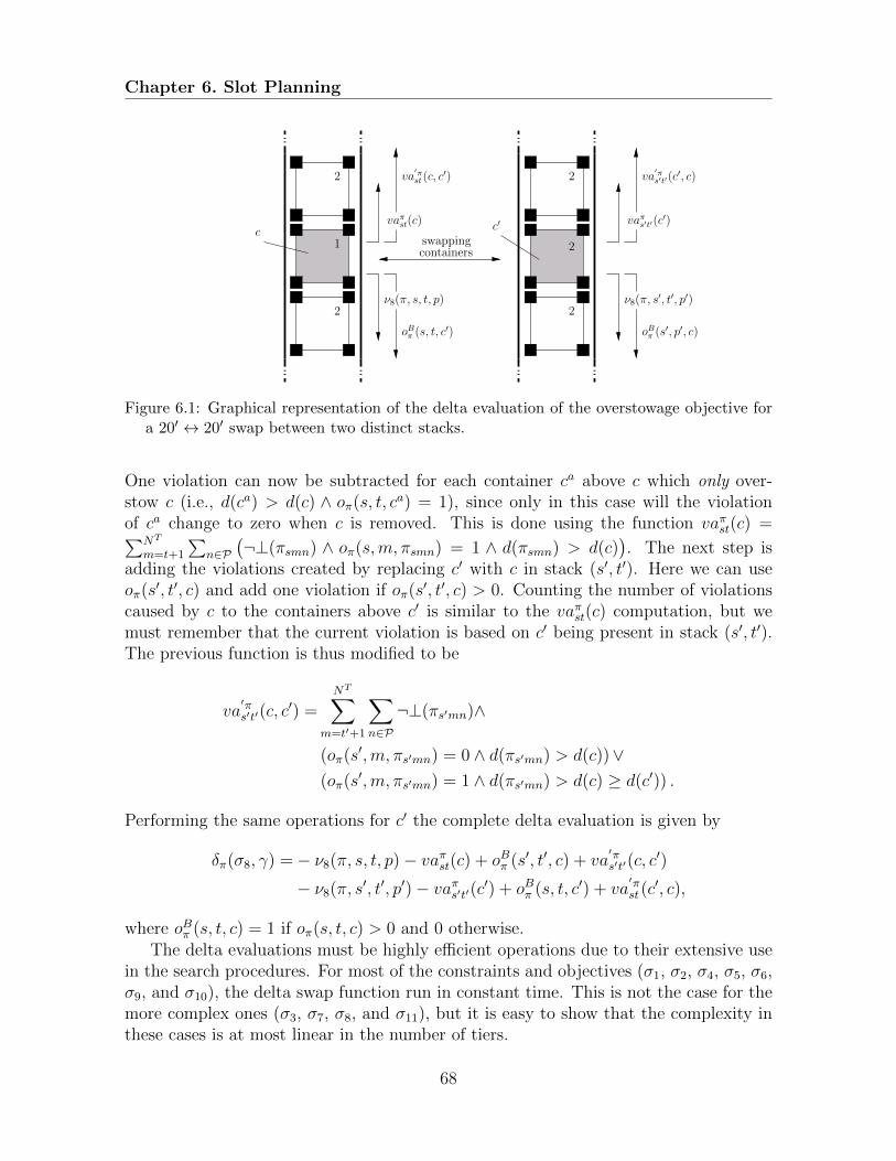
Chapter 6. Slot Planning
1
2
2
2
2
2
c c′
swappingcontainers
ν8(π, s, t, p)
va′πst(c, c
′)
vaπst(c)
ν8(π, s′, t′, p′)
oBπ (s, t, c′) oBπ (s′, p′, c)
vaπs′t′(c′)
va′πs′t′(c
′, c)
Figure 6.1: Graphical representation of the delta evaluation of the overstowage objective fora 20′ ↔ 20′ swap between two distinct stacks.
One violation can now be subtracted for each container ca above c which only over-stow c (i.e., d(ca) > d(c) ∧ oπ(s, t, ca) = 1), since only in this case will the violationof ca change to zero when c is removed. This is done using the function vaπst(c) =∑NT
m=t+1
∑n∈P
(¬⊥(πsmn) ∧ oπ(s,m, πsmn) = 1 ∧ d(πsmn) > d(c)
). The next step is
adding the violations created by replacing c′ with c in stack (s′, t′). Here we can useoπ(s′, t′, c) and add one violation if oπ(s′, t′, c) > 0. Counting the number of violationscaused by c to the containers above c′ is similar to the vaπst(c) computation, but wemust remember that the current violation is based on c′ being present in stack (s′, t′).The previous function is thus modified to be
va′πs′t′(c, c
′) =NT∑
m=t′+1
∑n∈P
¬⊥(πs′mn)∧
(oπ(s′,m, πs′mn) = 0 ∧ d(πs′mn) > d(c))∨(oπ(s′,m, πs′mn) = 1 ∧ d(πs′mn) > d(c) ≥ d(c′)) .
Performing the same operations for c′ the complete delta evaluation is given by
δπ(σ8, γ) =− ν8(π, s, t, p)− vaπst(c) + oBπ (s′, t′, c) + va′πs′t′(c, c
′)
− ν8(π, s′, t′, p′)− vaπs′t′(c′) + oBπ (s, t, c′) + va′πst(c
′, c),
where oBπ (s, t, c) = 1 if oπ(s, t, c) > 0 and 0 otherwise.The delta evaluations must be highly efficient operations due to their extensive use
in the search procedures. For most of the constraints and objectives (σ1, σ2, σ4, σ5, σ6,σ9, and σ10), the delta swap function run in constant time. This is not the case for themore complex ones (σ3, σ7, σ8, and σ11), but it is easy to show that the complexity inthese cases is at most linear in the number of tiers.
68
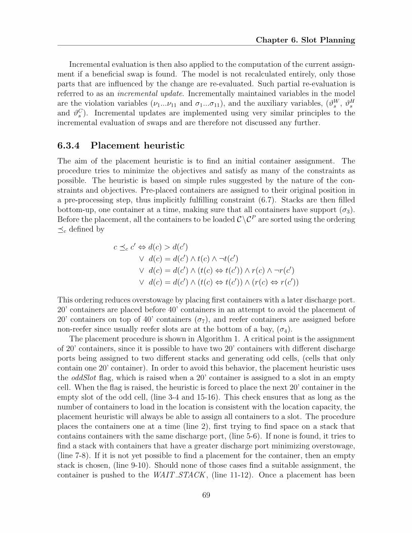
Chapter 6. Slot Planning
Incremental evaluation is then also applied to the computation of the current assign-ment if a beneficial swap is found. The model is not recalculated entirely, only thoseparts that are influenced by the change are re-evaluated. Such partial re-evaluation isreferred to as an incremental update. Incrementally maintained variables in the modelare the violation variables (ν1...ν11 and σ1...σ11), and the auxiliary variables, (ϑWs , ϑHsand ϑCs ). Incremental updates are implemented using very similar principles to theincremental evaluation of swaps and are therefore not discussed any further.
6.3.4 Placement heuristic
The aim of the placement heuristic is to find an initial container assignment. Theprocedure tries to minimize the objectives and satisfy as many of the constraints aspossible. The heuristic is based on simple rules suggested by the nature of the con-straints and objectives. Pre-placed containers are assigned to their original position ina pre-processing step, thus implicitly fulfilling constraint (6.7). Stacks are then filledbottom-up, one container at a time, making sure that all containers have support (σ3).Before the placement, all the containers to be loaded C\CP are sorted using the ordering�c defined by
c �c c′ ⇔ d(c) > d(c′)
∨ d(c) = d(c′) ∧ t(c) ∧ ¬t(c′)∨ d(c) = d(c′) ∧ (t(c)⇔ t(c′)) ∧ r(c) ∧ ¬r(c′)∨ d(c) = d(c′) ∧ (t(c)⇔ t(c′)) ∧ (r(c)⇔ r(c′))
This ordering reduces overstowage by placing first containers with a later discharge port.20’ containers are placed before 40’ containers in an attempt to avoid the placement of20’ containers on top of 40’ containers (σ7), and reefer containers are assigned beforenon-reefer since usually reefer slots are at the bottom of a bay, (σ4).
The placement procedure is shown in Algorithm 1. A critical point is the assignmentof 20’ containers, since it is possible to have two 20’ containers with different dischargeports being assigned to two different stacks and generating odd cells, (cells that onlycontain one 20’ container). In order to avoid this behavior, the placement heuristic usesthe oddSlot flag, which is raised when a 20’ container is assigned to a slot in an emptycell. When the flag is raised, the heuristic is forced to place the next 20’ container in theempty slot of the odd cell, (line 3-4 and 15-16). This check ensures that as long as thenumber of containers to load in the location is consistent with the location capacity, theplacement heuristic will always be able to assign all containers to a slot. The procedureplaces the containers one at a time (line 2), first trying to find space on a stack thatcontains containers with the same discharge port, (line 5-6). If none is found, it tries tofind a stack with containers that have a greater discharge port minimizing overstowage,(line 7-8). If it is not yet possible to find a placement for the container, then an emptystack is chosen, (line 9-10). Should none of those cases find a suitable assignment, thecontainer is pushed to the WAIT STACK , (line 11-12). Once a placement has been
69
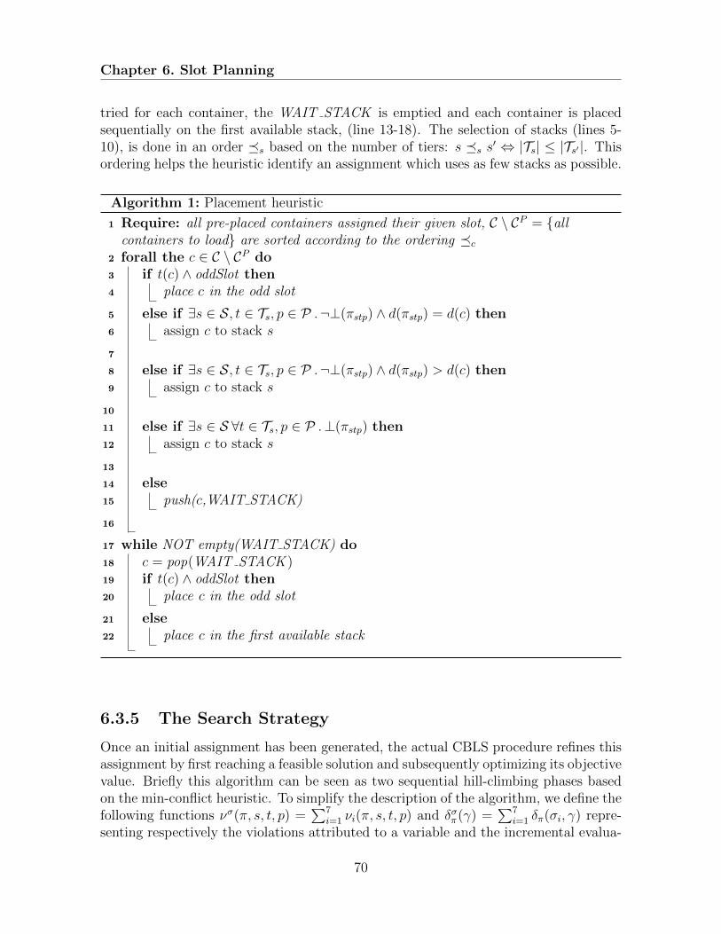
Chapter 6. Slot Planning
tried for each container, the WAIT STACK is emptied and each container is placedsequentially on the first available stack, (line 13-18). The selection of stacks (lines 5-10), is done in an order �s based on the number of tiers: s �s s′ ⇔ |Ts| ≤ |Ts′ |. Thisordering helps the heuristic identify an assignment which uses as few stacks as possible.
Algorithm 1: Placement heuristic
1 Require: all pre-placed containers assigned their given slot, C \ CP = {allcontainers to load} are sorted according to the ordering �c
2 forall the c ∈ C \ CP do3 if t(c) ∧ oddSlot then4 place c in the odd slot
5 else if ∃s ∈ S, t ∈ Ts, p ∈ P .¬⊥(πstp) ∧ d(πstp) = d(c) then6 assign c to stack s
7
8 else if ∃s ∈ S, t ∈ Ts, p ∈ P .¬⊥(πstp) ∧ d(πstp) > d(c) then9 assign c to stack s
10
11 else if ∃s ∈ S ∀t ∈ Ts, p ∈ P .⊥(πstp) then12 assign c to stack s
13
14 else15 push(c,WAIT STACK)
16
17 while NOT empty(WAIT STACK) do18 c = pop(WAIT STACK )19 if t(c) ∧ oddSlot then20 place c in the odd slot
21 else22 place c in the first available stack
6.3.5 The Search Strategy
Once an initial assignment has been generated, the actual CBLS procedure refines thisassignment by first reaching a feasible solution and subsequently optimizing its objectivevalue. Briefly this algorithm can be seen as two sequential hill-climbing phases basedon the min-conflict heuristic. To simplify the description of the algorithm, we define thefollowing functions νσ(π, s, t, p) =
∑7i=1 νi(π, s, t, p) and δσπ(γ) =
∑7i=1 δπ(σi, γ) repre-
senting respectively the violations attributed to a variable and the incremental evalua-
70

Chapter 6. Slot Planning
tion of a possible swap. And similarly for the objectives νo(π, s, t, p) =∑11
i=8 νi(π, s, t, p)and δoπ(γ) =
∑11i=8 δπ(σi, γ).
The general search procedure is outlined in Algorithm 2. It is important to noticethat the swap selection is done through the selection of two slots, where a slot is definedby the triple τ = 〈s, t, p〉, where s is the stack, t is the tier, and p is the position of theslot. Let T denote the set of all slot triples. The function Γ(τ, τ ′) : T × T 7→ Γ thendefines the swap based on the containers found in the two slots defined by τ and τ ′.
Algorithm 2: CBLS algorithm
1 sideMove ← false2 π = placementHeuristic()
3 while∑7
i=1 σi > 0 do4 π′ ← π5 selectMax s ∈ S, t ∈ Ts, p ∈ P on νσ(π, s, t, p) do6 selectMin s′ ∈ S, t′ ∈ Ts, p′ ∈ P on δσπ(γ = Γ(〈s, t, p〉, 〈s′, t′, p′〉)) do7 π ← swap(π, γ)
8 sideMove ← σ(π′) = σ(π)
9 changed = true10 sideMove = 011 while changed ∧ sideMoveCount < MAX SIDEMOVES do12 changed = false13 selectMax s ∈ S, t ∈ Ts, p ∈ P on νo(π, s, t, p) do14 select s′ ∈ S, t′ ∈ Ts, p′ ∈ P do15 changed = true on δoπ(γ = Γ(〈s, t, p〉, 〈s′, t′, p′〉))16 π = swap(π, γ)17 sideMove = 0
18 if ¬changed then19 select s′ ∈ S, t′ ∈ Ts, p′ ∈ P on eval oπ(γ = Γ(〈s, t, p〉, 〈s′, t′, p′〉)) do20 sideMove ← sideMove + 121 changed = true22 π = swap(π, γ)
23 return π;
The algorithm starts with the initial candidate assignment returned by the place-ment heuristic on line 2, and then performs the first hill-climbing CBLS over the neigh-borhood until all the constraints are satisfied, (line 3-8). The step function, whichselects a new assignment, makes the selection of the slots that will define the swap intwo phases. It begins (line 5), by selecting a slot triple τ = 〈s, t, p〉 preventing, however,the selection of slots holding pre-placed containers or null containers, and selects onlythose that actually violate some constraints. Between all the possible slots the one that
71
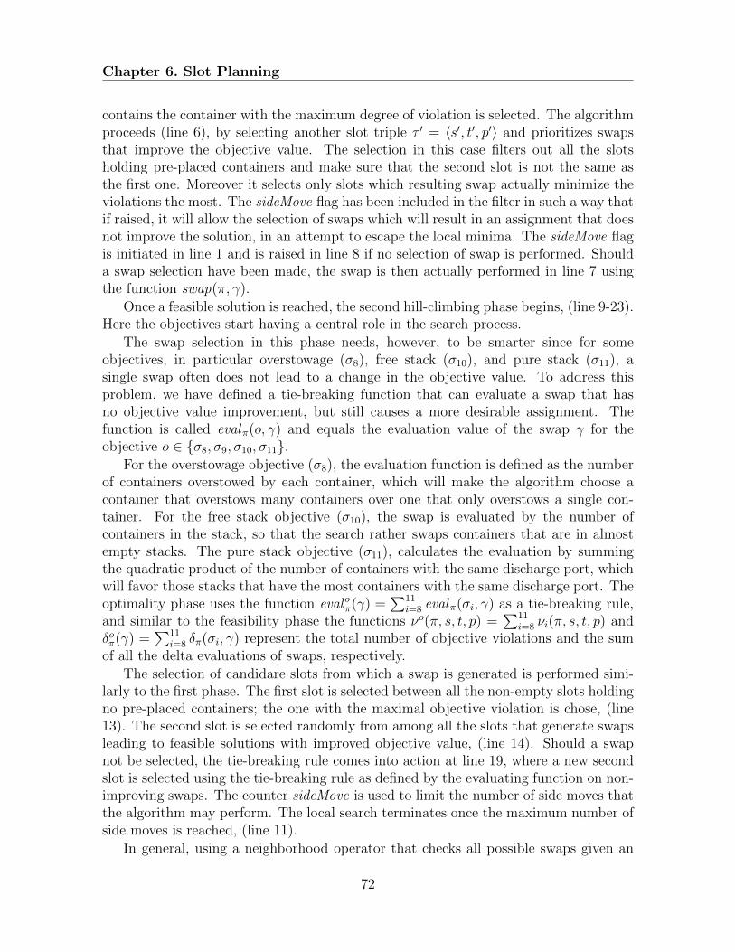
Chapter 6. Slot Planning
contains the container with the maximum degree of violation is selected. The algorithmproceeds (line 6), by selecting another slot triple τ ′ = 〈s′, t′, p′〉 and prioritizes swapsthat improve the objective value. The selection in this case filters out all the slotsholding pre-placed containers and make sure that the second slot is not the same asthe first one. Moreover it selects only slots which resulting swap actually minimize theviolations the most. The sideMove flag has been included in the filter in such a way thatif raised, it will allow the selection of swaps which will result in an assignment that doesnot improve the solution, in an attempt to escape the local minima. The sideMove flagis initiated in line 1 and is raised in line 8 if no selection of swap is performed. Shoulda swap selection have been made, the swap is then actually performed in line 7 usingthe function swap(π, γ).
Once a feasible solution is reached, the second hill-climbing phase begins, (line 9-23).Here the objectives start having a central role in the search process.
The swap selection in this phase needs, however, to be smarter since for someobjectives, in particular overstowage (σ8), free stack (σ10), and pure stack (σ11), asingle swap often does not lead to a change in the objective value. To address thisproblem, we have defined a tie-breaking function that can evaluate a swap that hasno objective value improvement, but still causes a more desirable assignment. Thefunction is called evalπ(o, γ) and equals the evaluation value of the swap γ for theobjective o ∈ {σ8, σ9, σ10, σ11}.
For the overstowage objective (σ8), the evaluation function is defined as the numberof containers overstowed by each container, which will make the algorithm choose acontainer that overstows many containers over one that only overstows a single con-tainer. For the free stack objective (σ10), the swap is evaluated by the number ofcontainers in the stack, so that the search rather swaps containers that are in almostempty stacks. The pure stack objective (σ11), calculates the evaluation by summingthe quadratic product of the number of containers with the same discharge port, whichwill favor those stacks that have the most containers with the same discharge port. Theoptimality phase uses the function eval oπ(γ) =
∑11i=8 evalπ(σi, γ) as a tie-breaking rule,
and similar to the feasibility phase the functions νo(π, s, t, p) =∑11
i=8 νi(π, s, t, p) andδoπ(γ) =
∑11i=8 δπ(σi, γ) represent the total number of objective violations and the sum
of all the delta evaluations of swaps, respectively.
The selection of candidare slots from which a swap is generated is performed simi-larly to the first phase. The first slot is selected between all the non-empty slots holdingno pre-placed containers; the one with the maximal objective violation is chose, (line13). The second slot is selected randomly from among all the slots that generate swapsleading to feasible solutions with improved objective value, (line 14). Should a swapnot be selected, the tie-breaking rule comes into action at line 19, where a new secondslot is selected using the tie-breaking rule as defined by the evaluating function on non-improving swaps. The counter sideMove is used to limit the number of side moves thatthe algorithm may perform. The local search terminates once the maximum number ofside moves is reached, (line 11).
In general, using a neighborhood operator that checks all possible swaps given an
72
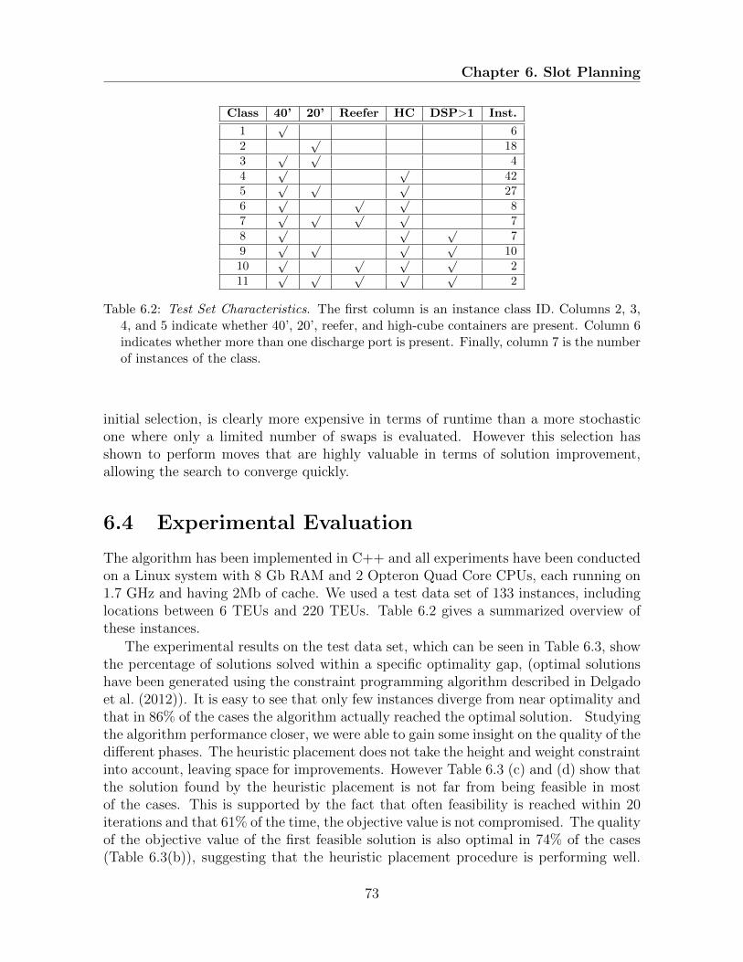
Chapter 6. Slot Planning
Class 40’ 20’ Reefer HC DSP>1 Inst.
1√
62
√18
3√ √
44
√ √42
5√ √ √
276
√ √ √8
7√ √ √ √
78
√ √ √7
9√ √ √ √
1010
√ √ √ √2
11√ √ √ √ √
2
Table 6.2: Test Set Characteristics. The first column is an instance class ID. Columns 2, 3,4, and 5 indicate whether 40’, 20’, reefer, and high-cube containers are present. Column 6indicates whether more than one discharge port is present. Finally, column 7 is the numberof instances of the class.
initial selection, is clearly more expensive in terms of runtime than a more stochasticone where only a limited number of swaps is evaluated. However this selection hasshown to perform moves that are highly valuable in terms of solution improvement,allowing the search to converge quickly.
6.4 Experimental Evaluation
The algorithm has been implemented in C++ and all experiments have been conductedon a Linux system with 8 Gb RAM and 2 Opteron Quad Core CPUs, each running on1.7 GHz and having 2Mb of cache. We used a test data set of 133 instances, includinglocations between 6 TEUs and 220 TEUs. Table 6.2 gives a summarized overview ofthese instances.
The experimental results on the test data set, which can be seen in Table 6.3, showthe percentage of solutions solved within a specific optimality gap, (optimal solutionshave been generated using the constraint programming algorithm described in Delgadoet al. (2012)). It is easy to see that only few instances diverge from near optimality andthat in 86% of the cases the algorithm actually reached the optimal solution. Studyingthe algorithm performance closer, we were able to gain some insight on the quality of thedifferent phases. The heuristic placement does not take the height and weight constraintinto account, leaving space for improvements. However Table 6.3 (c) and (d) show thatthe solution found by the heuristic placement is not far from being feasible in mostof the cases. This is supported by the fact that often feasibility is reached within 20iterations and that 61% of the time, the objective value is not compromised. The qualityof the objective value of the first feasible solution is also optimal in 74% of the cases(Table 6.3(b)), suggesting that the heuristic placement procedure is performing well.
73
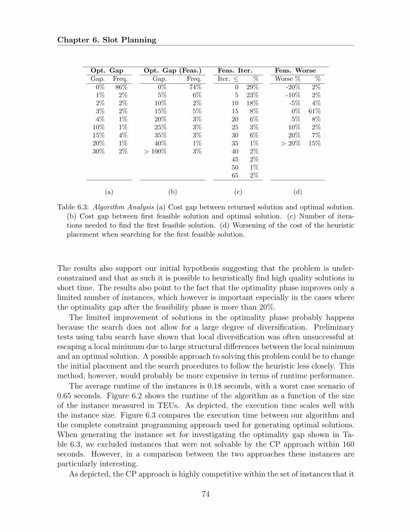
Chapter 6. Slot Planning
Opt. GapGap. Freq.
0% 86%1% 2%2% 2%3% 2%4% 1%
10% 1%15% 4%20% 1%30% 2%
(a)
Opt. Gap (Feas.)Gap. Freq.
0% 74%5% 6%
10% 2%15% 5%20% 3%25% 3%35% 3%40% 1%
> 100% 3%
(b)
Feas. Iter.Iter. ≤ %
0 29%5 23%
10 18%15 8%20 6%25 3%30 6%35 1%40 2%45 2%50 1%65 2%
(c)
Feas. WorseWorse % %
-20% 2%-10% 2%-5% 4%0% 61%5% 8%
10% 2%20% 7%
> 20% 15%
(d)
Table 6.3: Algorithm Analysis (a) Cost gap between returned solution and optimal solution.(b) Cost gap between first feasible solution and optimal solution. (c) Number of itera-tions needed to find the first feasible solution. (d) Worsening of the cost of the heuristicplacement when searching for the first feasible solution.
The results also support our initial hypothesis suggesting that the problem is under-constrained and that as such it is possible to heuristically find high quality solutions inshort time. The results also point to the fact that the optimality phase improves only alimited number of instances, which however is important especially in the cases wherethe optimality gap after the feasibility phase is more than 20%.
The limited improvement of solutions in the optimality phase probably happensbecause the search does not allow for a large degree of diversification. Preliminarytests using tabu search have shown that local diversification was often unsuccessful atescaping a local minimum due to large structural differences between the local minimumand an optimal solution. A possible approach to solving this problem could be to changethe initial placement and the search procedures to follow the heuristic less closely. Thismethod, however, would probably be more expensive in terms of runtime performance.
The average runtime of the instances is 0.18 seconds, with a worst case scenario of0.65 seconds. Figure 6.2 shows the runtime of the algorithm as a function of the sizeof the instance measured in TEUs. As depicted, the execution time scales well withthe instance size. Figure 6.3 compares the execution time between our algorithm andthe complete constraint programming approach used for generating optimal solutions.When generating the instance set for investigating the optimality gap shown in Ta-ble 6.3, we excluded instances that were not solvable by the CP approach within 160seconds. However, in a comparison between the two approaches these instances areparticularly interesting.
As depicted, the CP approach is highly competitive within the set of instances that it
74

Chapter 6. Slot Planning
Runtime
TEUs
Runtime performance
Tim
e (s
ec.)
0.7
0.6
0.5
0.4
0.3
0.2
0.1
00 50 100 150 200 250
Figure 6.2: Execution time as a function of instance size measured in TEUs.
LS vs CP runtime comparison
CP t
ime
LS time
NormalUnsolved
More than 5 sec.More then 3 sec.
1
0.8
0.6
0.4
0.2
00 0.2 0.4 0.6 0.8 1
Figure 6.3: Execution time comparison between our algorithm and the complete constraintprogramming approach used to generate optimal solutions.
can solve in 160 seconds. However our approach can solve the problematic instances forCP fast as well. This result indicates that the under-constrained nature of the problemmight force exact methods to spend an excessive amount of time proving optimality.
6.5 Dealing with Fractional and Infeasible Instances
As mentioned before, the abstracted decisions taken during master planning might re-sult in infeasible slot planning instances. CBLS is of great help in this situation, since,thanks to the concept of constraint violations, it is possible to analyse an infeasibleinstance. Once the feasibility phase fails, the resulting solution is one where the viola-tions have been minimized. This means that the solution is the one closest to feasibilitythat the algorithm could find. We then find a feasible solution using algorithm 3.
The algorithm selects the variable with the highest degree of violation (line 2), and
75
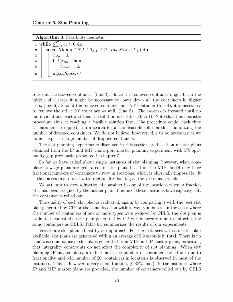
Chapter 6. Slot Planning
Algorithm 3: Feasibility heuristic
1 while∑7
i=1 σi > 0 do2 selectMax s ∈ S, t ∈ Ts, p ∈ P on νσ(π, s, t, p) do3 xstp = ⊥4 if t(xstp) then5 xstp−1 = ⊥6 adjustStack(s)
rolls out the stowed container, (line 3). Since the removed container might be in themiddle of a stack it might be necessary to lower down all the containers in highertiers, (line 6). Should the removed container be a 20’ container (line 4), it is necessaryto remove the other 20’ container as well, (line 5). The process is iterated until nomore violations exist and thus the solution is feasible, (line 1). Note that this heuristicprocedure aims at reaching a feasible solution fast. The procedure could, each timea container is dropped, run a search for a new feasible solution thus minimizing thenumber of dropped containers. We do not believe, however, this to be necessary as wedo not expect a large number of dropped containers.
The slot planning experiments discussed in this section are based on master plansobtained from the IP and MIP multi-port master planning experiment with 5% opti-mality gap previously presented in chapter 5.
So far we have talked about single instances of slot planning, however, when com-plete stowage plans are generated, master plans based on the MIP model may havefractional numbers of containers to stow in locations, which is physically impossible. Itis thus necessary to deal with fractionality looking at the vessel as a whole.
We attempt to stow a fractioned container in one of the locations where a fractionof it has been assigned by the master plan. If none of these locations have capacity left,the container is rolled out.
The quality of each slot plan is evaluated, again, by comparing it with the best slotplan generated by CP for the same location within twenty minutes. In the cases wherethe number of containers of one or more types were reduced by CBLS, the slot plan isevaluated against the best plan generated by CP within twenty minutes, stowing thesame containers as CBLS. Table 6.4 summarizes the results of our experiments.
Vessels are slot planned fast by our approach. For the instances with a master planavailable, slot plans are generated within an average of 5.9 seconds in total. There is notime-wise dominance of slot plans generated from MIP and IP master plans, indicatingthat integrality constraints do not affect the complexity of slot planning. When slotplanning IP master plans, a reduction in the number of containers rolled out due tofractionality and odd number of 20’ containers in locations is observed in most of theinstances. This is, however, a very small fraction, (0.88% max). In the instances whereIP and MIP master plans are provided, the number of containers rolled out by CBLS
76
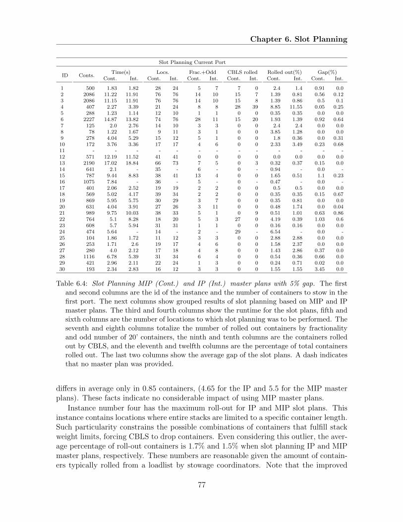
Chapter 6. Slot Planning
Slot Planning Current Port
ID Conts.Time(s) Locs. Frac.+Odd CBLS rolled Rolled out(%) Gap(%)
Cont. Int. Cont. Int. Cont. Int. Cont. Int. Cont. Int. Cont. Int.
1 500 1.83 1.82 28 24 5 7 7 0 2.4 1.4 0.91 0.02 2086 11.22 11.91 76 76 14 10 15 7 1.39 0.81 0.56 0.123 2086 11.15 11.91 76 76 14 10 15 8 1.39 0.86 0.5 0.14 407 2.27 3.39 21 24 8 8 28 39 8.85 11.55 0.05 0.255 288 1.23 1.14 12 10 1 1 0 0 0.35 0.35 0.0 0.06 2227 14.87 13.82 74 76 28 11 15 20 1.93 1.39 0.92 0.647 125 2.0 2.76 14 10 3 3 0 0 2.4 2.4 0.0 0.08 78 1.22 1.67 9 11 3 1 0 0 3.85 1.28 0.0 0.09 278 4.04 5.29 15 12 5 1 0 0 1.8 0.36 0.0 0.3110 172 3.76 3.36 17 17 4 6 0 0 2.33 3.49 0.23 0.6811 - - - - - - - - - - - - -12 571 12.19 11.52 41 41 0 0 0 0 0.0 0.0 0.0 0.013 2190 17.02 18.84 66 73 7 5 0 3 0.32 0.37 0.15 0.014 641 2.1 - 35 - 6 - 0 - 0.94 - 0.0 -15 787 9.44 8.83 38 41 13 4 0 0 1.65 0.51 1.1 0.2316 1075 7.84 - 36 - 5 - 0 - 0.47 - 0.0 -17 401 2.06 2.52 19 19 2 2 0 0 0.5 0.5 0.0 0.018 569 5.02 4.17 39 34 2 2 0 0 0.35 0.35 0.15 0.6719 869 5.95 5.75 30 29 3 7 0 0 0.35 0.81 0.0 0.020 631 4.04 3.91 27 26 3 11 0 0 0.48 1.74 0.0 0.0421 989 9.75 10.03 38 33 5 1 0 9 0.51 1.01 0.63 0.8622 764 5.1 8.28 18 20 5 3 27 0 4.19 0.39 1.03 0.623 608 5.7 5.94 31 31 1 1 0 0 0.16 0.16 0.0 0.024 474 5.64 - 14 - 2 - 29 - 6.54 - 0.0 -25 104 1.86 1.72 11 12 3 3 0 0 2.88 2.88 0.0 0.026 253 1.71 2.6 19 17 4 6 0 0 1.58 2.37 0.0 0.027 280 4.0 2.12 17 18 4 8 0 0 1.43 2.86 0.37 0.028 1116 6.78 5.39 31 34 6 4 0 0 0.54 0.36 0.66 0.029 421 2.96 2.11 22 24 1 3 0 0 0.24 0.71 0.02 0.030 193 2.34 2.83 16 12 3 3 0 0 1.55 1.55 3.45 0.0
Table 6.4: Slot Planning MIP (Cont.) and IP (Int.) master plans with 5% gap. The firstand second columns are the id of the instance and the number of containers to stow in thefirst port. The next columns show grouped results of slot planning based on MIP and IPmaster plans. The third and fourth columns show the runtime for the slot plans, fifth andsixth columns are the number of locations to which slot planning was to be performed. Theseventh and eighth columns totalize the number of rolled out containers by fractionalityand odd number of 20’ containers, the ninth and tenth columns are the containers rolledout by CBLS, and the eleventh and twelfth columns are the percentage of total containersrolled out. The last two columns show the average gap of the slot plans. A dash indicatesthat no master plan was provided.
differs in average only in 0.85 containers, (4.65 for the IP and 5.5 for the MIP masterplans). These facts indicate no considerable impact of using MIP master plans.
Instance number four has the maximum roll-out for IP and MIP slot plans. Thisinstance contains locations where entire stacks are limited to a specific container length.Such particularity constrains the possible combinations of containers that fulfill stackweight limits, forcing CBLS to drop containers. Even considering this outlier, the aver-age percentage of roll-out containers is 1.7% and 1.5% when slot planning IP and MIPmaster plans, respectively. These numbers are reasonable given the amount of contain-ers typically rolled from a loadlist by stowage coordinators. Note that the improved
77
Chapter 6. Slot Planning
weight constraints in the master planning model with ballast tanks (see Section 5.4),would solve this particular issue since specific weight constraints are considered for eachcontainer length.
Of the slot plans generated for the IP and MIP master plans 2.24% have an opti-mality gap over 5%, and only 1.24% a gap over 10%. The maximum gap, however, is55%. CP generated optimal slot plans within one second for 96.2% of the locations ofthe MIP master plans and 96.0% of the locations of the IP ones. Moreover, CP wasable to prove optimality 87.8% and 86.5% of the slot plans generated for the locationsfor the MIP and IP master plans, respectively.
78

Chapter 7. Conclusions
Chapter 7
Conclusions
The aim of this thesis has been to investigate the possibility of applying automatedstowage planning in practice. The work presented does not aim to show that stowagecoordinators can be substituted by automated planners, but rather to explore the pos-sibility of using automatically generated stowage plans in decision support tools forstowage coordinators. In order to answer the research question, two main aspects ofautomated stowage planning were to be taken into account. First, the quality of thegenerated solution and second, the performance of the system in terms of runtime. Toensure the generated solutions are of high quality, we have proposed a representativemodel in collaboration with the industry. This representative problem includes all therelevant computational components of container stowage planning and all the detailsthat make the solutions of this problem possible to evaluate by stowage coordinators.The representative problem requires the handling of vessel stability and stress forces,the consideration of 20’ and 40’ containers and all their stacking rules, and the opti-mization of overstowage and crane utilization.
The algorithmic approach presented in this thesis hierarchically decomposes theproblem into a master planning and a slot planning phase. During the master planningphase, groups of containers are assigned to sub-sections of the vessel. During thisphase, stability and stress forces are solved, and hatch-overstowage and crane utilizationare optimized. The slot planning phase, solves the stowage problem of each location,handling stacking constraints and optimizing overstowage. This decomposition, and theruntime performance of the two phases, is able to solve large scale container stowageproblems within 10 minutes, which is the time limit given by the industry for a toolto be useful within the day to day planning routine of stowage coordinators. Furtherimprovements of the master planning model were presented in this thesis that analysedthe possibility of including ballast tanks in the optimization model.
The experimental results collected in this thesis show that automated stowage planscan be generated for the representative problem within the 10 minute time frame set bythe industry, thus giving a positive answer to the research question central to this thesis.Moreover, it has been shown that ballast water can be successfully modelled usingstandard mathematical programming methods via the use of linearization of hydrostatic
79

Chapter 7. Conclusions
data. The possibility of modelling such problems with standard modelling tools providesthe industry with the flexibility of easily adding side-constraints and changing theobjectives.
7.1 Outlook and Future Directions
This thesis has shown a proof of concept that container stowage planning can be au-tomated, resulting in solutions of high quality within a short time. The integrationof such a system within the planning process of stowage coordinators is an interestingdirection for future research. In order for current state-of-the-art container stowageplanning to be part of the daily work routine, a number of extensions are needed, suchas the handling of lashing forces and support for special requirement container types.It is debatable whether those extensions should be a part of the optimization modelor if they should be included into an external decision process. The modality in whichoptimization models integrate into daily work routines can be a fascinating challengeas they will have to be able to handle the heuristic choices and quality criterions thatmight change between coordinators. In this direction, the work of Jensen et al. (2012)is the first to apply configuration ideas to the container stowage problem, where binarydecision diagrams are used to guide the user.
Besides extensions to the current approach, some of the results obtained indicateother interesting research directions in terms of the general approach taken. Consider,for example, the runtime performance of the two phases. It might be possible to ex-change information between the two phases such that a true optimal solution can befound. Now consider the master planning phase which includes the planning of downstream ports. Cargo flow information for such ports is based on forecast data, whichis more imprecise the further down the stream the plan goes. An interesting futureanalysis would be to use a rolling horizon optimization and study how it impacts thesolutions. Such an approach could greatly improve the runtime of the master planningphase.
Stowage Planning in Artificial Intelligence
A very different research direction can be the analysis of the knowledge of stowagecoordinators. Successful approaches to stowage planning, such as the one used in thisthesis, are based on the work process of stowage coordinators. It is not always simple,however, to extract this knowledge, as different heuristic rules might be used by differentcoordinators. Systematic analysis of historical data might allow learning algorithms toinfer heuristic rules which can be applied to improve the current models. An examplecould be to estimate the distribution of containers with the same discharge port ona vessel given a loadlist and a release. Such information could be used as branchingheuristics, thus boosting the solution process.
80

Chapter 7. Conclusions
Stowage Planning in Related Problems
Container stowage planning can be seen as a central element of many decisions in theliner shipping industry. The fact that it can be solved within acceptable time limitsopens the opportunity of solving other problems that depend on stowage planning.Cargo flow analysis over the strings of a liner shipping network could benefit from theintegration of stowage planning, as it would be possible to analyse the feasibility of thecargo flows based on the vessels deployed in more detail than the raw TEU capacityof a vessel. Heuristically generated stowage plans could then also be implemented intosimulation models for the analysis of business decisions, for example in network designor repositioning.
81
Chapter 7. Conclusions
82
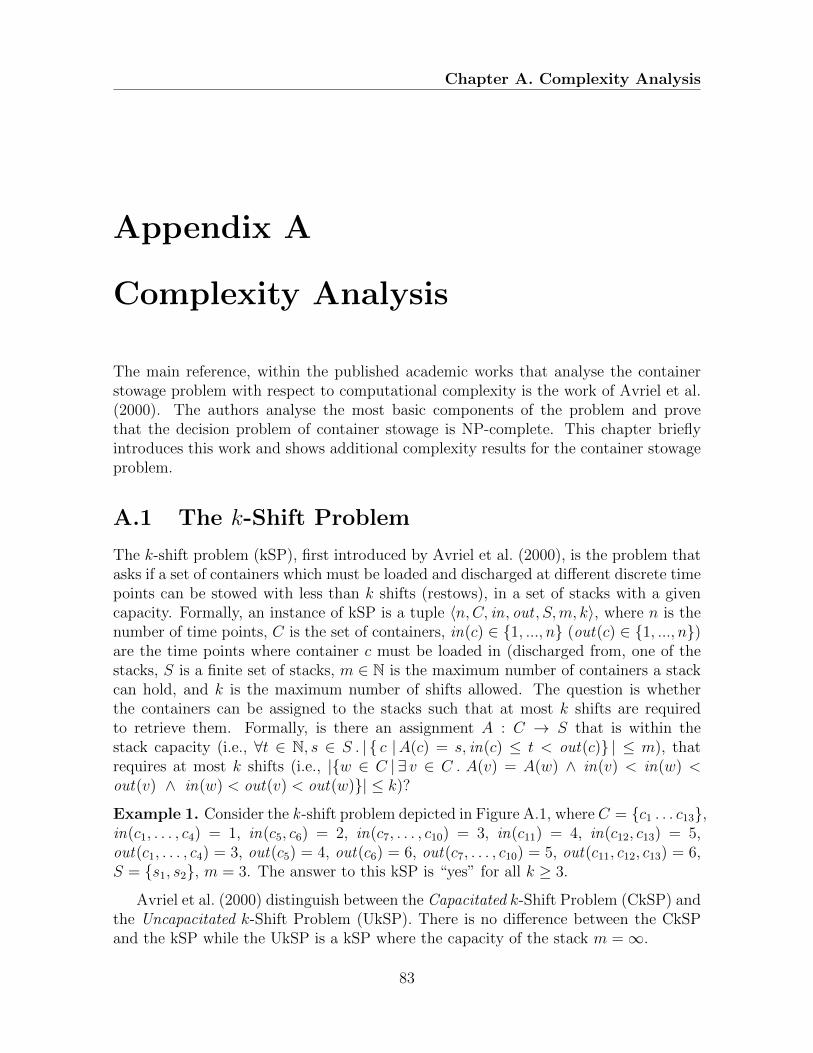
Chapter A. Complexity Analysis
Appendix A
Complexity Analysis
The main reference, within the published academic works that analyse the containerstowage problem with respect to computational complexity is the work of Avriel et al.(2000). The authors analyse the most basic components of the problem and provethat the decision problem of container stowage is NP-complete. This chapter brieflyintroduces this work and shows additional complexity results for the container stowageproblem.
A.1 The k-Shift Problem
The k-shift problem (kSP), first introduced by Avriel et al. (2000), is the problem thatasks if a set of containers which must be loaded and discharged at different discrete timepoints can be stowed with less than k shifts (restows), in a set of stacks with a givencapacity. Formally, an instance of kSP is a tuple 〈n,C, in, out , S,m, k〉, where n is thenumber of time points, C is the set of containers, in(c) ∈ {1, ..., n} (out(c) ∈ {1, ..., n})are the time points where container c must be loaded in (discharged from, one of thestacks, S is a finite set of stacks, m ∈ N is the maximum number of containers a stackcan hold, and k is the maximum number of shifts allowed. The question is whetherthe containers can be assigned to the stacks such that at most k shifts are requiredto retrieve them. Formally, is there an assignment A : C → S that is within thestack capacity (i.e., ∀t ∈ N, s ∈ S . | { c |A(c) = s, in(c) ≤ t < out(c)} | ≤ m), thatrequires at most k shifts (i.e., |{w ∈ C | ∃ v ∈ C . A(v) = A(w) ∧ in(v) < in(w) <out(v) ∧ in(w) < out(v) < out(w)}| ≤ k)?
Example 1. Consider the k -shift problem depicted in Figure A.1, where C = {c1 . . . c13},in(c1, . . . , c4) = 1, in(c5, c6) = 2, in(c7, . . . , c10) = 3, in(c11) = 4, in(c12, c13) = 5,out(c1, . . . , c4) = 3, out(c5) = 4, out(c6) = 6, out(c7, . . . , c10) = 5, out(c11, c12, c13) = 6,S = {s1, s2}, m = 3. The answer to this kSP is “yes” for all k ≥ 3.
Avriel et al. (2000) distinguish between the Capacitated k-Shift Problem (CkSP) andthe Uncapacitated k-Shift Problem (UkSP). There is no difference between the CkSPand the kSP while the UkSP is a kSP where the capacity of the stack m =∞.
83

Chapter A. Complexity Analysis
Figure A.1: A kSP instance with m = 3. The instance is a “yes”-instance for any k ≥ 3.Possible configurations (disregarding symmetric ones), are shown at each time step withthe discharge time of the container in each slot. Gray slots contain containers that mustbe shifted, and each configuration is labeled with the number of containers that will beshifted at that time-step. A path through the configurations represents a complete stowageplan, and the optimal plan is shown with bold arcs.
A.2 UkSP is NP-Complete
The NP-completeness of the UkSP is proven by Avriel et al. (2000) via a reductionfrom the circle-graph coloring problem. Avriel et al. (2000) shows that a special caseof the UkSP, where k = 0, is equivalent to the circle-graph coloring problem and thusknown complexity results can be easily applied to the U(zero)SP. Avriel et al. (2000)shows how a circle-graph can be constructed from an instance of a U(zero)SP wherethe number of colors on the circle-graph coloring problem corresponds to the numberof stacks in the U(zero)SP. The authors prove the following theorem:
Theorem 1. Let C be the number of columns in an uncapacitated bay. Then, theuncapacitated shift problem is NP-complete for C ≥ 4.
In this theorem C corresponds to the number of stacks |S| and an uncapacitatedbay corresponds to the set of stacks in S. Even though the authors base the proof onthe U(zero)SP, the result carries over to the UkSP since the U(zero)SP is a special caseof the UkSP. Due to the equivalence with the circle-graph coloring problem, it is alsoknown that the U(zero)SP is in P for any uncapacitated bays with less than 4 stacks.Beside Aslidis (1990) O(n3) algorithm for the UkSP with one stack, the complexity ofUkSP for two and three stacks is still an open problem.
A short coming, in terms of practical use of the result, of theorem 1 is that, as theauthors have hinted, if |S| ≥ |P | the problem becomes trivially solvable in polynomialtime since stacks can be dedicated to a single discharge port. A more precise theoremwould then be:
84
Chapter A. Complexity Analysis
c
h
c
h
c
c
c
1
2
4
2
1
3
5
h
h1
2
c
c
c
c
1
2
3
4
c5
h2
h1
(b)(a)
1 2 3 4 5 6 7 8 9 1 2 3 4 5 6 7 8 9
Figure A.2: (a) A HOP instance with m = 2 and k = 1. (b) An assignment of containers tohatches with only one hatch overstow (for h1) showing that it is a “yes”-instance.
Theorem 2. Let C be the number of columns in an uncapacitated bay and P be thenumber of ports visited. Then, the uncapacitated shift problem is NP-complete for 4 ≤C < |P |.
A.3 Complexity of CkSP
Avriel et al. (2000) extends the complexity result of the UkSP of to the CkSP, since apolynomial reduction from UkSP is trivia, (it is enough to set m = |C| to simulate anuncapacitated stack). The authors therefore show that the CkSP is NP-complete.
Theorem 3. Let C be the number of stacks of capacity m in a bay. The capacitatedk-shifts problem is NP-complete for all m > 1 and C ≥ 4.
A.4 The Hatch Overstow Problem
In Chapter 2, the concept of hatch-overstowage was introduced. As this problem sig-nificantly impacts the total number of re-handles, it is of interest to analyze it’s com-putational complexity. We perform this analysis defining the Hatch Overstow Problem(HOP). HOP is a decision problem that asks whether a set of containers that mustbe loaded and discharged in a set of numbered ports visited, in the order 1, 2, . . ., canbe stowed on a set of hatch covers without causing more than k hatch overstows. Inparticular when the hatches may have to be removed in some ports to access containersstowed below them. Formally, an instance of the HOP is a tuple 〈C, in, out , H, r,m, k〉,where C is a finite set of containers; in(c) ∈ N (out(c) ∈ N) is the port that container cmust be loaded to (and unloaded from); H is a finite set of hatches; r(h) ∈ 2N is the setof ports where hatch h must be removed; m ∈ N is the maximum number of containersthat each hatch can hold at any time; and k ∈ {0, . . . , |C|} is the maximum number ofhatch overstows.
The question is whether the containers can be assigned to the hatches withoutcausing more than k hatch overstows. Formally, the question is whether there ex-
85
Chapter A. Complexity Analysis
ists an assignment A : C → H that is within the hatch capacity (i.e., ∀t ∈ N, h ∈H .∣∣ { c |A(c) = h, in(c) ≤ t < out(c)}
∣∣ ≤ m), and has at most k hatch overstows,(i.e.,
∣∣ { c | ∃p ∈ r(A(c)) . in(c) < p < out(c)}∣∣ ≤ k).
Example 2. Consider a HOP with C = {c1, c2, c3, c4, c5}, in(c1) = 1, in(c2) = 2,in(c3) = 4, in(c4) = 5, in(c5) = 5, out(c1) = 3, out(c2) = 6, out(c3) = 7, out(c4) = 8,out(c5) = 9, H = {h1, h2}, r(h1) = {2, 6, 8}, r(h2) = {4, 9}, m = 2, and k = 1. Asdepicted in Figure A.2, the answer to this HOP is “yes”.
We now prove that the HOP is NP-complete by a reduction from the Set CoverProblem (SCP). Recall that an instance of the SCP is a tuple 〈S,A, k′〉, where S isa finite set, A is a collection of non-empty subsets of S, and k′ ∈ {1, . . . , |A|}. Thequestion is whether A contains a cover for S of size k′ or less, i.e. a subset A′ ⊆ A with|A′| ≤ k′ such that every element of S belongs to at least one member of A.1
Example 3. Consider an SCP with A = {a1, a2, a3} where a1 = {e1, e3}, a2 = {e3, e4},and a3 = {e1, e2, e4}, S = {e1, e2, e3, e4}, k′ = 2. Clearly this is a “yes”-instance sinceS can be covered by A′ = {a1, a3}.
Theorem 4. The HOP is NP-complete.
Proof. We have HOP ∈ NP since the assignment A can be used as a certificatethat can be checked in polynomial time. We next prove that SCP ≤p HOP whichshows that the HOP is NP-hard. The reduction algorithm begins with an instance〈{e1, . . . , e|S|}, {a1, . . . , a|A|}, k′〉 of the SCP. We shall now construct a HOP instance〈C, in, out , H, r,m, k〉 that has an assignment with no more than k hatch overstows if,and only if, the SCP instance has a cover with a size no greater than k′. The HOPinstance is constructed by reducing the hatch capacity to one and using the containers torepresent the elements in S as well as using the hatches to represent A. The idea is thata container that belongs to a subset can be assigned to a hatch representing it withoutcausing overstowage. To measure the size of these non-overstowing covers, |A| blockingcontainers and k′ extra hatches are introduced. Formally, we have C = S∪{b1, . . . , b|A|},where 〈in(ei), out(ei)〉 = 〈2i−1, 2i+1〉 for 1 ≤ i ≤ |S| and 〈in(bi), out(bi)〉 = 〈1, 2|S|+1〉for 1 ≤ i ≤ |A|. Further, H = A ∪ {f1, . . . , fk}, where r(ai) = {2j | ej ∈ S \ ai} for1 ≤ i ≤ |A| and r(bi) = {2j | ej ∈ S} for 1 ≤ i ≤ k. Finally, we have m = 1 andk = |A|. Clearly, this HOP instance can be constructed in polynomial time. As anexample of the construction, Figure A.3 shows the HOP instance of the SCP defined inExample 3.
We must show that this transformation of SCP into HOP is a reduction. First sup-pose that the SCP has a cover A′ = {a′1, . . . , a′n} where n ≤ k′. For the correspondingHOP, assign each container representing an element in S to a hatch representing asubset in the cover that includes it. This is possible with m = 1 because none of these
1There are slight variations of the SCP in the literature. The one used here differs from SP5 inGarey and Johnson (1979) by requiring that the subsets of A are non-empty. It is trivial to show thatSCP is NP-complete by a reduction from SP5.
86
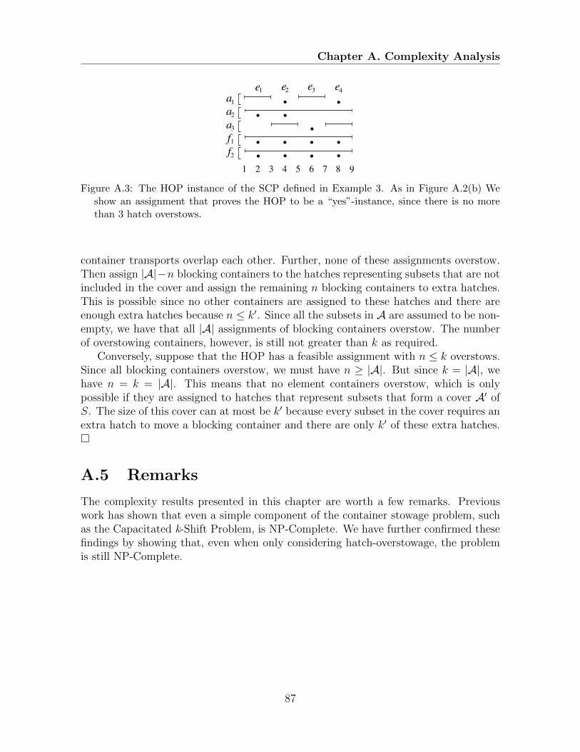
Chapter A. Complexity Analysis
1 2 3 4 5 6 7 98
e e e e4321
a
a
2
1
a1
2
3
f
f
Figure A.3: The HOP instance of the SCP defined in Example 3. As in Figure A.2(b) Weshow an assignment that proves the HOP to be a “yes”-instance, since there is no morethan 3 hatch overstows.
container transports overlap each other. Further, none of these assignments overstow.Then assign |A|−n blocking containers to the hatches representing subsets that are notincluded in the cover and assign the remaining n blocking containers to extra hatches.This is possible since no other containers are assigned to these hatches and there areenough extra hatches because n ≤ k′. Since all the subsets in A are assumed to be non-empty, we have that all |A| assignments of blocking containers overstow. The numberof overstowing containers, however, is still not greater than k as required.
Conversely, suppose that the HOP has a feasible assignment with n ≤ k overstows.Since all blocking containers overstow, we must have n ≥ |A|. But since k = |A|, wehave n = k = |A|. This means that no element containers overstow, which is onlypossible if they are assigned to hatches that represent subsets that form a cover A′ ofS. The size of this cover can at most be k′ because every subset in the cover requires anextra hatch to move a blocking container and there are only k′ of these extra hatches.�
A.5 Remarks
The complexity results presented in this chapter are worth a few remarks. Previouswork has shown that even a simple component of the container stowage problem, suchas the Capacitated k-Shift Problem, is NP-Complete. We have further confirmed thesefindings by showing that, even when only considering hatch-overstowage, the problemis still NP-Complete.
87
Chapter A. Complexity Analysis
88

Chapter B. Decomposition in Scheduling
Appendix B
Decomposition in Scheduling
This appendix presents the results of a collaboration with Professor Pascal Van Hen-tenryck. The aim of the collaboration was to explore the application of constraintbased decomposition frameworks on scheduling problems, specifically on the flexiblejobshop problem. Particular attention is given to the Adaptive Randomized Decompo-sition (ARD) framework that was applied to these problems for the first time.
B.1 Constraint Based Decompositions for Schedul-
ing Problems
Constraint-based schedulers have been widely successful in modeling and solving com-plex industrial scheduling applications. They provide a general-purpose approach toapplications involving complex resources and constraints. Moreover, in recent years,the combination of Constraint Based Scheduler (CBS) and local search techniques (e.g.,large neighborhood search or iterative flattening), has been instrumental in obtaininghigh-quality solutions quickly and improving best-known solutions in a variety of pureproblems such as cumulative scheduling and open-shop problems.
This research considers the application of constraint-based scheduling to flexiblejobshop problems, a generalization of the traditional jobshop scheduling where activi-ties have a choice of machines. Flexible jobshops are quite challenging, since they addanother level of decisions and reduce the power of filtering algorithms for disjunctiveresources. In particular, this paper studies both Large Neighborhood Search (LNS),and ARD inspired by research on large-scale vehicle-routing applications. LNS usesrandom, temporal, and machine neighborhoods, while ARD exploits temporal and ma-chine decouplings to produce subproblems that can be optimized separately.
Empirical results on some standard benchmarks show that, within 5 minutes, bothLNS and ARD produce many new best solutions and are about 0.5% on average fromthe best-known solutions. Furthermore, over longer runtimes, they improve 61% of thebest-known solutions and match the remaining ones. The empirical results also showthe importance of hybrid neighborhoods and decompositions in LNS and ARD.
89
Chapter B. Decomposition in Scheduling
These results are obtained with a rather naive CBS search, which requires little de-velopment effort on top of a modern constraint-based scheduling and does not useadvanced search heuristics or learning techniques. As a consequence, they furtherdemonstrate the versatility of the general-purpose approach of combining CBS withlocal search and decomposition schemes. The ARD schemes are also shown to be closein quality and efficiency to LNS, indicating that they are likely to provide high-qualitysolutions to large-scale problems which cannot be handled globally.
B.2 The Flexible Jobshop Problem
A flexible jobshop is specified by a set of jobs, each of which consists of a sequence ofactivities. Each activity can execute on a set of machines, each with a possibly differentduration. No two activities can execute on the same machine at the same time andthe goal is to minimize the makespan, i.e., the completion date of all activities. Moreformally, each activity a has a set M(a) of machines on which it can execute and a dura-tion d(a,m) for each machine m ∈M(a). Every job defined by a sequence of activities〈a1, ..., an〉 generates a set of precedence constraints (ai−1, ai) for i ≥ 2. We use A todenote the set of activities, P the set of precedence constraints, and M the set of ma-chines. The time horizon H for the schedule is given by
[0,∑
a∈Amaxm∈M(a) d(a,m)].
A solution to the flexible jobshop is a pair of assignments (σ, µ), where µ : A 7→Massigns a machine µ(a) ∈ M(a) to each activity a and σ : A 7→ H assigns a startingdate σ(a) to each activity a. A solution is feasible if it satisfies the precedence andcapacity constraints, i.e.,
∀(ai, aj) ∈ P : σ(aj) ≥ σ(ai) + d(ai, µ(ai))∀m ∈M, t ∈ H : |A(σ,m, t)| ≤ 1
where A(σ,m, t) is the set of activities assigned to machine m at time t, i.e.,
{a ∈ A | µ(a) = m ∧ σ(a) ≤ t ≤ σ(a) + d(a, µ(a))} .
An optimal solution is a feasible solution (σ, µ) minimizing
maxa∈A σ(a) + d(a, µ(a)).
We also use ω(a) to denote σ(a) + d(a, µ(a)) in this paper.
B.3 Prior Work
Approaches to solve flexible shop problems are often divided between hierarchical andsimultaneous searches. Hierarchical heuristics (Akella and Gershwin, 1984; Bona et al.,1990; Brandimarte, 1993; Escudero, 1989), are based on the property that, given amachine assignment, the objective function can be optimized solving a classic jobshop
90
Chapter B. Decomposition in Scheduling
problem. Simultaneous approaches (Barnes and Chambers, 1996; Brucker and Neyer,1998; Jurisch, 1992; Hurink et al., 1994; Vaessens, 1995; Mastrolilli and Gambardella,2000; Hmida et al., 2007, 2010; Gao, 2008; Pezzella et al., 2008), tend to identify neigh-borhoods which either solve the routing and the assignment into different transactions(Barnes and Chambers, 1996; Brucker and Schlie, 1990; Jurisch, 1992; Hurink et al.,1994; Hmida et al., 2007, 2010), or at the same time, (Dauzere-Peres and Paulli, 1997;Vaessens, 1995; Mastrolilli and Gambardella, 2000; Gao, 2008; Pezzella et al., 2008).Specifically to the benchmarks used in this paper, Mastrolilli and Gambardella (2000)proposed a tabu search procedure using two neighborhoods functions defined by themoving of an operation and its feasible or optimal insertions, improving a large num-ber of the best-known upper bounds. A hybrid search combining genetic and variableneighborhood descent algorithms was implemented by Gao (2008), reporting betterperformance than the tabu search. However, details of new upper bounds have notbeen reported. A constraint programming approach was developed by Hmida et al.(2010) using discrepancy search but the results are dominated by both Mastrolilli andGambardella (2000) and Gao (2008).
B.4 A Constraint-Based Scheduling Model
A simple CBS formulation for the flexible shop is shown in Figure B.1, (using a Comet-like syntax). Lines 1–5 initialize the constants, i.e., the set of activities and machines,the durations, the set of machines required by each activity, and the set of precedenceconstraints. Lines 6 and 7 define the decision variables as activity objects, which canbe queried for their starting and ending dates. Line 8 defines a pool of unary resourceswhich maintain the machine selection of each activity and the capacity constraints usingedge-finder and NotFirst/NotLast propagators. Line 9 declares the array of selectedmachines for each activity, (see also lines 20–21). Lines 11–22 define the objectivefunction and the constraints of the problem. The search procedure is specified in lines24–30 and is rather naive. It starts by branching over the machine selection variables,considering activities with the fewest machines first, (lines 24–26). The machines arethen ranked, starting with those with the least slack (lines 27–28), before assigning theearliest starting dates to all activities, (lines 29–30).
B.5 Large Neighborhood Search
LNS is a combination of Local Search and CP, which has proved effective in solvinglarge-scale combinatorial optimization problems. The search procedure is based on adestruction/construction principle. Once an initial solution is found, part of the vari-able assignments are relaxed (destruction), while keeping the remaining variables fixed.A new solution is then found by re-optimizing the assignment of the free variables, (con-struction). These two steps are then iterated until some termination criterion. Whenapplied to scheduling problems, it is beneficial to impose only precedence constraints
91
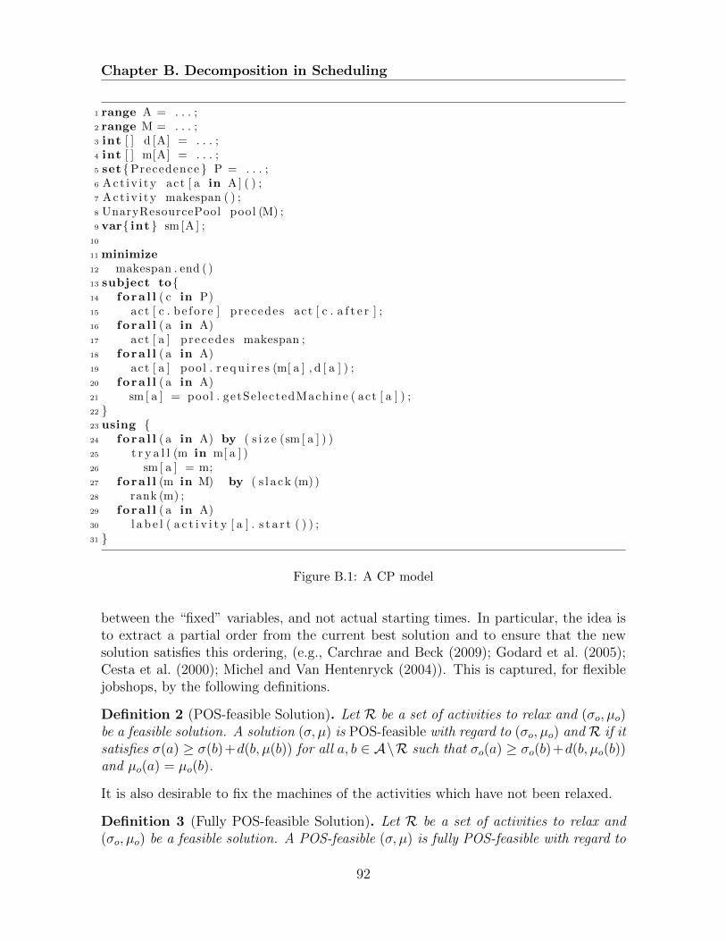
Chapter B. Decomposition in Scheduling
1 range A = . . . ;2 range M = . . . ;3 int [ ] d [A] = . . . ;4 int [ ] m[A] = . . . ;5 set{Precedence } P = . . . ;6 Act iv i ty act [ a in A] ( ) ;7 Act iv i ty makespan ( ) ;8 UnaryResourcePool pool (M) ;9 var{ int} sm [A ] ;
10
11 minimize12 makespan . end ( )13 subject to{14 f o ra l l ( c in P)15 act [ c . b e f o r e ] precedes act [ c . a f t e r ] ;16 f o ra l l ( a in A)17 act [ a ] precedes makespan ;18 f o ra l l ( a in A)19 act [ a ] pool . r e q u i r e s (m[ a ] , d [ a ] ) ;20 f o ra l l ( a in A)21 sm [ a ] = pool . getSe lectedMachine ( act [ a ] ) ;22 }23 using {24 f o ra l l ( a in A) by ( s i z e (sm [ a ] ) )25 t r y a l l (m in m[ a ] )26 sm [ a ] = m;27 f o ra l l (m in M) by ( s l a c k (m) )28 rank (m) ;29 f o ra l l ( a in A)30 l a b e l ( a c t i v i t y [ a ] . s t a r t ( ) ) ;31 }
Figure B.1: A CP model
between the “fixed” variables, and not actual starting times. In particular, the idea isto extract a partial order from the current best solution and to ensure that the newsolution satisfies this ordering, (e.g., Carchrae and Beck (2009); Godard et al. (2005);Cesta et al. (2000); Michel and Van Hentenryck (2004)). This is captured, for flexiblejobshops, by the following definitions.
Definition 2 (POS-feasible Solution). Let R be a set of activities to relax and (σo, µo)be a feasible solution. A solution (σ, µ) is POS-feasible with regard to (σo, µo) and R if itsatisfies σ(a) ≥ σ(b)+d(b, µ(b)) for all a, b ∈ A\R such that σo(a) ≥ σo(b)+d(b, µo(b))and µo(a) = µo(b).
It is also desirable to fix the machines of the activities which have not been relaxed.
Definition 3 (Fully POS-feasible Solution). Let R be a set of activities to relax and(σo, µo) be a feasible solution. A POS-feasible (σ, µ) is fully POS-feasible with regard to
92
Chapter B. Decomposition in Scheduling
(σo, µo) and R if it is POS-feasible with regard to (σo, µo) and R and satisfies µ(a) =µo(a) ∧ µ(b) = µo(b) for all a, b ∈ A \ R.
The neighborhoods in this paper only consider fully POS-feasible solutions and aregeneralizations of those used in Carchrae and Beck (2009). They differ on the choice ofthe set R of activities to relax and whether or not some additional machine constraintsare placed on the relaxed activities. Three main neighborhoods are considered:
1. The random neighborhood: The set R is a random set of activities.
2. The time-window neighborhood: A time window [α, β] is chosen randomly and Ris the set of all activities in the interval [α, β].
3. The machine neighborhood: A set of machines is selected randomly and R is theset of all activities on those machines.
Moreover, three additional neighborhoods are constructed from these by selecting asubset R ⊆ R and imposing the constraint: ∀a ∈ R : µ(a) = µo(a).
B.6 Adaptive Randomized Decompositions
The concept of Adaptive Randomized Decomposition (ARD) was proposed in Bentand Van Hentenryck (2010) to tackle large scale vehicle routing problems. Its aim is tofind a sequence of decouplings, i.e., subproblems that can be independently optimizedand whose solution can be merged back into an existing solution to produce a bettersolution. Formally, given an instance P of a flexible shop problem, the idea is to usethe current solution π to find a decoupling (Po, Ps) with projected solution πo and πs.The problem Po is then re-optimized and its solution is merged into πs to obtain a newsolution for P . The ARD thus follows two simple principles:
1. Starting from an initial solution π0 of P , it produces a sequence of solutionsπ1, ..., πn such that the objective function f(π0) ≥ f(π1) ≥ ... ≥ f(πn).
2. At step i, the solution πi−1 is used to obtain the decoupling (Po, Ps) of P withsolutions πo and πs. The problem Po is then re-optimized and its solution π∗o isused to obtain the new solution of πi = MERGE(π∗o , πi−1).
The choice of algorithms for optimizing the sub-problems is independent from the ARDscheme. Our results were obtained by using CP and LNS algorithms.
B.6.1 Time Decomposition
The time decomposition extracts a subproblem consisting of the activities that lie withina time window 〈s, e〉.
93
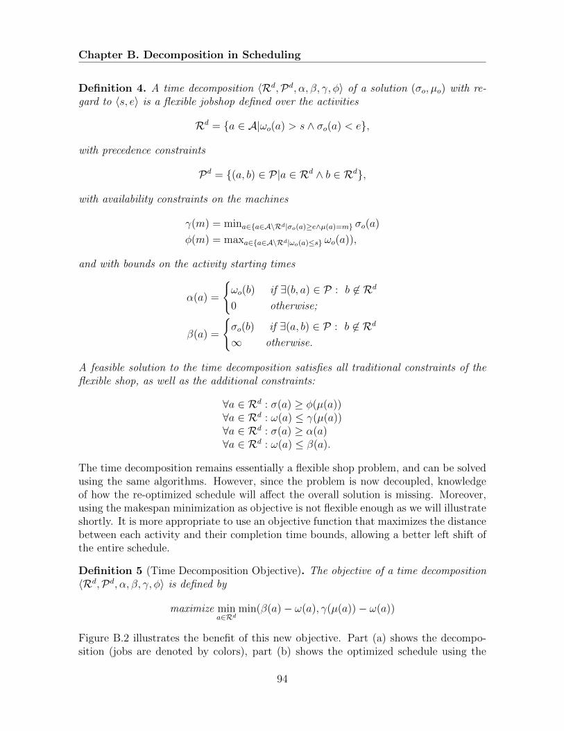
Chapter B. Decomposition in Scheduling
Definition 4. A time decomposition 〈Rd,Pd, α, β, γ, φ〉 of a solution (σo, µo) with re-gard to 〈s, e〉 is a flexible jobshop defined over the activities
Rd = {a ∈ A|ωo(a) > s ∧ σo(a) < e},
with precedence constraints
Pd = {(a, b) ∈ P|a ∈ Rd ∧ b ∈ Rd},
with availability constraints on the machines
γ(m) = mina∈{a∈A\Rd|σo(a)≥e∧µ(a)=m} σo(a)
φ(m) = maxa∈{a∈A\Rd|ωo(a)≤s} ωo(a)),
and with bounds on the activity starting times
α(a) =
{ωo(b) if ∃(b, a) ∈ P : b 6∈ Rd
0 otherwise;
β(a) =
{σo(b) if ∃(a, b) ∈ P : b 6∈ Rd
∞ otherwise.
A feasible solution to the time decomposition satisfies all traditional constraints of theflexible shop, as well as the additional constraints:
∀a ∈ Rd : σ(a) ≥ φ(µ(a))∀a ∈ Rd : ω(a) ≤ γ(µ(a))∀a ∈ Rd : σ(a) ≥ α(a)∀a ∈ Rd : ω(a) ≤ β(a).
The time decomposition remains essentially a flexible shop problem, and can be solvedusing the same algorithms. However, since the problem is now decoupled, knowledgeof how the re-optimized schedule will affect the overall solution is missing. Moreover,using the makespan minimization as objective is not flexible enough as we will illustrateshortly. It is more appropriate to use an objective function that maximizes the distancebetween each activity and their completion time bounds, allowing a better left shift ofthe entire schedule.
Definition 5 (Time Decomposition Objective). The objective of a time decomposition〈Rd,Pd, α, β, γ, φ〉 is defined by
maximize mina∈Rd
min(β(a)− ω(a), γ(µ(a))− ω(a))
Figure B.2 illustrates the benefit of this new objective. Part (a) shows the decompo-sition (jobs are denoted by colors), part (b) shows the optimized schedule using the
94
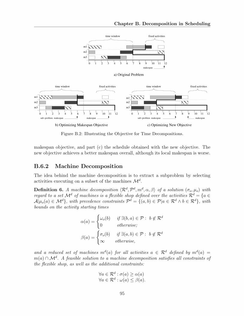
Chapter B. Decomposition in Scheduling
c) Optimizing New Objective
0 1 12111098765432
m3
m2
m1
time window fixed activities
makespan
a) Original Problem
0 1 2 3 4 5 6 7 8 9 10 11 12
m3
m1
m2
time window fixed activities
sub−problem makespan makespan
b) Optimizing Makespan Objective
0 1 2 3 4 5 6 7 8 9 10 11 12
m3
m2
m1
makespansub−problem makespan
fixed activitiestime window
Figure B.2: Illustrating the Objective for Time Decompositions.
makespan objective, and part (c) the schedule obtained with the new objective. Thenew objective achieves a better makespan overall, although its local makespan is worse.
B.6.2 Machine Decomposition
The idea behind the machine decomposition is to extract a subproblem by selectingactivities executing on a subset of the machines Md.
Definition 6. A machine decomposition 〈Rd,Pd,md, α, β〉 of a solution (σo, µo) withregard to a set Md of machines is a flexible shop defined over the activities Rd = {a ∈A|µo(a) ∈ Md}, with precedence constraints Pd = {(a, b) ∈ P|a ∈ Rd ∧ b ∈ Rd}, withbounds on the activity starting times
α(a) =
{ωo(b) if ∃(b, a) ∈ P : b 6∈ Rd
0 otherwise;
β(a) =
{σo(b) if ∃(a, b) ∈ P : b 6∈ Rd
∞ otherwise,
and a reduced set of machines md(a) for all activities a ∈ Rd defined by md(a) =m(a) ∩Md. A feasible solution to a machine decomposition satisfies all constraints ofthe flexible shop, as well as the additional constraints:
∀a ∈ Rd : σ(a) ≥ α(a)∀a ∈ Rd : ω(a) ≤ β(a).
95
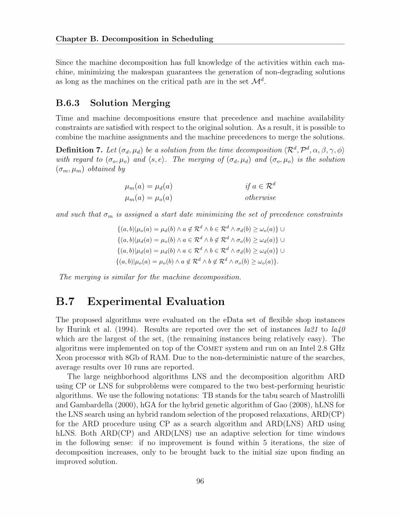
Chapter B. Decomposition in Scheduling
Since the machine decomposition has full knowledge of the activities within each ma-chine, minimizing the makespan guarantees the generation of non-degrading solutionsas long as the machines on the critical path are in the set Md.
B.6.3 Solution Merging
Time and machine decompositions ensure that precedence and machine availabilityconstraints are satisfied with respect to the original solution. As a result, it is possible tocombine the machine assignments and the machine precedences to merge the solutions.
Definition 7. Let (σd, µd) be a solution from the time decomposition 〈Rd,Pd, α, β, γ, φ〉with regard to (σo, µo) and 〈s, e〉. The merging of (σd, µd) and (σo, µo) is the solution(σm, µm) obtained by
µm(a) = µd(a) if a ∈ Rd
µm(a) = µo(a) otherwise
and such that σm is assigned a start date minimizing the set of precedence constraints
{(a, b)|µo(a) = µd(b) ∧ a 6∈ Rd ∧ b ∈ Rd ∧ σd(b) ≥ ωo(a)} ∪{(a, b)|µd(a) = µo(b) ∧ a ∈ Rd ∧ b 6∈ Rd ∧ σo(b) ≥ ωd(a)} ∪{(a, b)|µd(a) = µd(b) ∧ a ∈ Rd ∧ b ∈ Rd ∧ σd(b) ≥ ωd(a)} ∪{(a, b)|µo(a) = µo(b) ∧ a 6∈ Rd ∧ b 6∈ Rd ∧ σo(b) ≥ ωo(a)}.
The merging is similar for the machine decomposition.
B.7 Experimental Evaluation
The proposed algorithms were evaluated on the eData set of flexible shop instancesby Hurink et al. (1994). Results are reported over the set of instances la21 to la40which are the largest of the set, (the remaining instances being relatively easy). Thealgoritms were implemented on top of the Comet system and run on an Intel 2.8 GHzXeon processor with 8Gb of RAM. Due to the non-deterministic nature of the searches,average results over 10 runs are reported.
The large neighborhood algorithms LNS and the decomposition algorithm ARDusing CP or LNS for subproblems were compared to the two best-performing heuristicalgorithms. We use the following notations: TB stands for the tabu search of Mastrolilliand Gambardella (2000), hGA for the hybrid genetic algorithm of Gao (2008), hLNS forthe LNS search using an hybrid random selection of the proposed relaxations, ARD(CP)for the ARD procedure using CP as a search algorithm and ARD(LNS) ARD usinghLNS. Both ARD(CP) and ARD(LNS) use an adaptive selection for time windowsin the following sense: if no improvement is found within 5 iterations, the size ofdecomposition increases, only to be brought back to the initial size upon finding animproved solution.
96
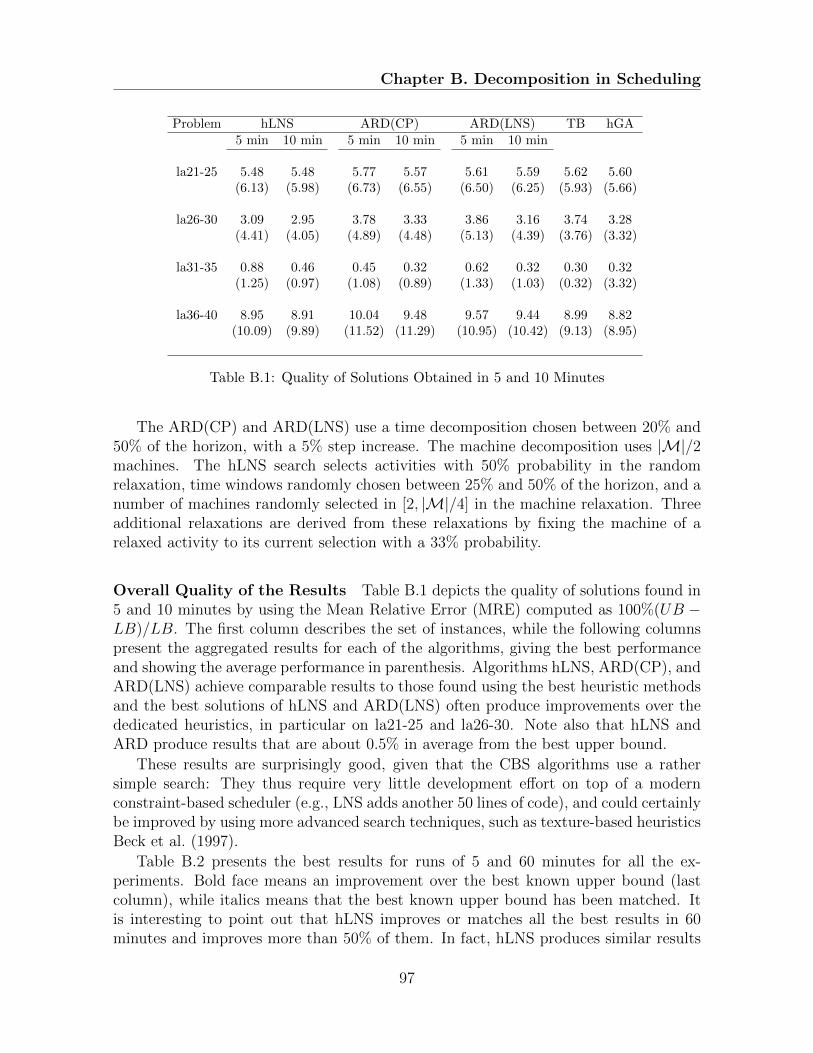
Chapter B. Decomposition in Scheduling
Problem hLNS ARD(CP) ARD(LNS) TB hGA5 min 10 min 5 min 10 min 5 min 10 min
la21-25 5.48 5.48 5.77 5.57 5.61 5.59 5.62 5.60(6.13) (5.98) (6.73) (6.55) (6.50) (6.25) (5.93) (5.66)
la26-30 3.09 2.95 3.78 3.33 3.86 3.16 3.74 3.28(4.41) (4.05) (4.89) (4.48) (5.13) (4.39) (3.76) (3.32)
la31-35 0.88 0.46 0.45 0.32 0.62 0.32 0.30 0.32(1.25) (0.97) (1.08) (0.89) (1.33) (1.03) (0.32) (3.32)
la36-40 8.95 8.91 10.04 9.48 9.57 9.44 8.99 8.82(10.09) (9.89) (11.52) (11.29) (10.95) (10.42) (9.13) (8.95)
Table B.1: Quality of Solutions Obtained in 5 and 10 Minutes
The ARD(CP) and ARD(LNS) use a time decomposition chosen between 20% and50% of the horizon, with a 5% step increase. The machine decomposition uses |M|/2machines. The hLNS search selects activities with 50% probability in the randomrelaxation, time windows randomly chosen between 25% and 50% of the horizon, and anumber of machines randomly selected in [2, |M|/4] in the machine relaxation. Threeadditional relaxations are derived from these relaxations by fixing the machine of arelaxed activity to its current selection with a 33% probability.
Overall Quality of the Results Table B.1 depicts the quality of solutions found in5 and 10 minutes by using the Mean Relative Error (MRE) computed as 100%(UB −LB)/LB. The first column describes the set of instances, while the following columnspresent the aggregated results for each of the algorithms, giving the best performanceand showing the average performance in parenthesis. Algorithms hLNS, ARD(CP), andARD(LNS) achieve comparable results to those found using the best heuristic methodsand the best solutions of hLNS and ARD(LNS) often produce improvements over thededicated heuristics, in particular on la21-25 and la26-30. Note also that hLNS andARD produce results that are about 0.5% in average from the best upper bound.
These results are surprisingly good, given that the CBS algorithms use a rathersimple search: They thus require very little development effort on top of a modernconstraint-based scheduler (e.g., LNS adds another 50 lines of code), and could certainlybe improved by using more advanced search techniques, such as texture-based heuristicsBeck et al. (1997).
Table B.2 presents the best results for runs of 5 and 60 minutes for all the ex-periments. Bold face means an improvement over the best known upper bound (lastcolumn), while italics means that the best known upper bound has been matched. Itis interesting to point out that hLNS improves or matches all the best results in 60minutes and improves more than 50% of them. In fact, hLNS produces similar results
97
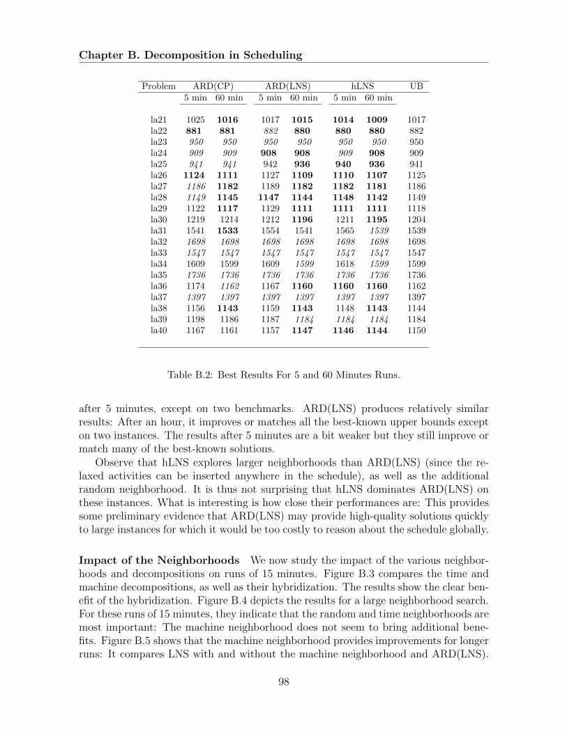
Chapter B. Decomposition in Scheduling
Problem ARD(CP) ARD(LNS) hLNS UB5 min 60 min 5 min 60 min 5 min 60 min
la21 1025 1016 1017 1015 1014 1009 1017la22 881 881 882 880 880 880 882la23 950 950 950 950 950 950 950la24 909 909 908 908 909 908 909la25 941 941 942 936 940 936 941la26 1124 1111 1127 1109 1110 1107 1125la27 1186 1182 1189 1182 1182 1181 1186la28 1149 1145 1147 1144 1148 1142 1149la29 1122 1117 1129 1111 1111 1111 1118la30 1219 1214 1212 1196 1211 1195 1204la31 1541 1533 1554 1541 1565 1539 1539la32 1698 1698 1698 1698 1698 1698 1698la33 1547 1547 1547 1547 1547 1547 1547la34 1609 1599 1609 1599 1618 1599 1599la35 1736 1736 1736 1736 1736 1736 1736la36 1174 1162 1167 1160 1160 1160 1162la37 1397 1397 1397 1397 1397 1397 1397la38 1156 1143 1159 1143 1148 1143 1144la39 1198 1186 1187 1184 1184 1184 1184la40 1167 1161 1157 1147 1146 1144 1150
Table B.2: Best Results For 5 and 60 Minutes Runs.
after 5 minutes, except on two benchmarks. ARD(LNS) produces relatively similarresults: After an hour, it improves or matches all the best-known upper bounds excepton two instances. The results after 5 minutes are a bit weaker but they still improve ormatch many of the best-known solutions.
Observe that hLNS explores larger neighborhoods than ARD(LNS) (since the re-laxed activities can be inserted anywhere in the schedule), as well as the additionalrandom neighborhood. It is thus not surprising that hLNS dominates ARD(LNS) onthese instances. What is interesting is how close their performances are: This providessome preliminary evidence that ARD(LNS) may provide high-quality solutions quicklyto large instances for which it would be too costly to reason about the schedule globally.
Impact of the Neighborhoods We now study the impact of the various neighbor-hoods and decompositions on runs of 15 minutes. Figure B.3 compares the time andmachine decompositions, as well as their hybridization. The results show the clear ben-efit of the hybridization. Figure B.4 depicts the results for a large neighborhood search.For these runs of 15 minutes, they indicate that the random and time neighborhoods aremost important: The machine neighborhood does not seem to bring additional bene-fits. Figure B.5 shows that the machine neighborhood provides improvements for longerruns: It compares LNS with and without the machine neighborhood and ARD(LNS).
98

Chapter B. Decomposition in Scheduling
1220
1240
1260
1280
1300
1320
1340
0 2 4 6 8 10 12 14 16
Ma
ke
sp
an
Minutes.
Time DecompositionMachine Decomposition
Hybrid Decomposition
Figure B.3: The Impact of the Decompositions.
1220
1230
1240
1250
1260
1270
1280
1290
1300
1310
0 2 4 6 8 10 12 14 16
Ma
ke
sp
an
Minutes.
Time & Machine NeighborhoodRandom & Time Neighborhood
Random & Machine NeighborhoodHybrid Neighborhood
Figure B.4: The Impact of the Neighborhoods.
The results indicate that the machine neighborhood starts improving the results after15 minutes and is necessary for LNS to dominate ARD(LNS). These results also shedsome interesting light on the strength of the decomposition approach, which does not
99
Chapter B. Decomposition in Scheduling
rely on the random neighborhood, giving us some reasonable confidence that it willscale nicely on large-scale instances.
1210
1220
1230
1240
1250
1260
1270
1280
0 10 20 30 40 50 60
Ma
ke
sp
an
Minutes.
ARD(LNS)hLNS without Machine Neighborhood
hLNS
Figure B.5: The Impact of the Neighborhoods over Long Runs.
B.8 Concluding Remarks
This appendix presented large neighborhood and adaptive randomized decompositionapproaches to the flexible jobshop problem. It demonstrated that a simple CBS formu-lation, enhanced with LNS or ARD, provides very high-quality results quickly on somestandard classes of benchmarks and requires little development effort on top of a mod-ern CBS system. Moreover, the approaches improved 60% of the best upper bounds,while matching the remaining ones. The quality of the decomposition approach indi-cates that it is likely to scale to large-scale problems for which considering the problemin its entirety is not feasible. These results were achieved without advanced heuristicsor learning techniques (Carchrae and Beck, 2009), suggesting that there is room forsignificant improvements. Overall, these results seem to confirm that LNS and ARDover a CBS formulation is an effective and general-purpose approach to many complexscheduling problems.
100
Chapter C. Completeness of the CBLS neighborhood
Appendix C
Completeness of the CBLSneighborhood
Proposition 3. The swap neighborhood Γ defined by the union of swap20 and swap40
swaps for a slot planning problem Π is complete.
Proof. We prove the claim by showing that any current assignment π of the variablesof Π can be changed to an arbitrary assignment π′ via a sequence of swaps. Let xπstpdenote the value of variable xstp in assignment π. Assume without loss of generalitythat the variables of Π are re-assigned from π to π′ according to some total ordering ofthe cells ≺. Consider assigning the variables of cell (s, t) at some point in this orderedre-assignment. We have two cases:
1. f(xπ′st1) (i.e., a 40’ container must be placed in the cell). If xπ
′st1 = xπst1 the cell
assignment is correct. Otherwise find the container xπ′st1 in a cell (s′, t′) and use
swap40 of type 1 to 5 to assign it to xst1.
2. ¬f(xπ′st1) (i.e., 20’ containers or empties must be placed in the cell). If xπ
′st1 = xπst1
then the aft slot of the cell is assigned correctly. Otherwise find the container(including ⊥), in the fore slot of the cell or in another cell (s′, t′) and use swap20
type 1 or 2 to assign it to xst1. Do the same for xst2, except only look for thecontainer in another cell (s′, t′).
Because all variables of cells previous to (s, t) have already been assigned, the cells(s′, t′) with containers to swap into (s, t) must come after (s, t) (i.e. (s, t) ≺ (s′, t′)).Since the cell (s, t) is arbitrarily chosen, all cells can be re-assigned from π to π′ usingthe resulting sequence of swaps.
101
Chapter C. Completeness of the CBLS neighborhood
102

BIBLIOGRAPHY
Bibliography
(2010). Storck Guide: Stowage& Segregation to IMDG Code. Storck Verlag Hamburg.
Akella, R. and S. Gershwin (1984, September). Performance of Hierarchical ProductionScheduling Policy. IEEE Transactions on Components, Hybrids, and ManufacturingTechnology 7 (3), 225–240.
Alphaliner (2012, 04). Top 100.
Ambrosino, D., D. Anghinolfi, M. Paolucci, and A. Sciomachen (2010). An experimentalcomparison of different heuristics for the master bay plan problem. In Proceedings ofthe 9th Int. Symposium on Experimental Algorithms, pp. 314–325.
Ambrosino, D. and A. Sciomachen (1998). A constraint satisfaction approach for masterbay plans. Maritime Engineering and Ports 36, 175–184.
Ambrosino, D. and A. Sciomachen (2003). Impact of yard organization on the masterbay planning problem. Maritime Economics and Logistics (5), 285–300.
Ambrosino, D., A. Sciomachen, D. Anghinolfi, and M. Paolucci (2009, March). Anew three-step heuristic for the master bay plan problem. Maritime Economics andLogistics 11 (1), 98–120.
Ambrosino, D., A. Sciomachen, and E. Tanfani (2004). Stowing a conteinership: themaster bay plan problem. Transportation Research Part A: Policy and Practice 38 (2),81–99.
Ambrosino, D., A. Sciomachen, and E. Tanfani (2006). A decomposition heuristics forthe container ship stowage problem. Journal of Heuristics 12 (3), 211–233.
Aslidis, A. (1990). Minimizing of overstowage in container ship operations. OperationalResearch 90, 457–471.
Aslidis, A. H. (1984). Optimal container loading. Master’s thesis, Massachusetts Insti-tute of Technology.
Aslidis, A. H. (1989). Combinatorial Algorithms for Stacking Problems. Ph. D. thesis,Massachusetts Institute of Technology.
103
BIBLIOGRAPHY
Avriel, M., M. Penn, and N. Shpirer (2000). Container ship stowage problem: complex-ity and connection to the coloring of circle graphs. Discrete Applied Mathematics 103,271–279.
Avriel, M., M. Penn, N. Shpirer, and S. Witteboon (1998). Stowage planning forcontainer ships to reduce the number of shifts. Annals of Operations Research 76,55–71.
Azevedo, A., C. Ribeiro, A. Chaves, G. Sena, L. Salles Neto, and A. Moretti (2012,February). Solving the 3d containership stowage loading planning problem by repre-sentation by rules and beam search. In Proceedings of the 1st International Conferenceon Operations Research and Enterprise Systems - ICORES 2012.
Barnes, W. J. and J. B. Chambers (1996). Flexible Job Shop Scheduling by TabuSearch.
Beck, J., A. Davenport, E. Sitarski, and M. Fox (1997). Texture-based heuristics forscheduling revisited. In Proceedings of the National Conference on Artificial Intelli-gence, pp. 241–248. Citeseer.
Bent, R. and P. Van Hentenryck (2010). Spatial, Temporal, and Hybrid Decompositionsfor Large-Scale Vehicle Routing with Time Windows. In D. Cohen (Ed.), Principlesand Practice of Constraint Programming, Volume 6308 of Lecture Notes in ComputerScience, Berlin, Heidelberg, pp. 99–113–113. Springer Berlin Heidelberg.
Bona, B., P. Brandimarte, C. Greco, and G. Menga (1990). Hybrid hierarchical schedul-ing and control systems in manufacturing. IEEE Transactions on Robotics and Au-tomation 6 (6), 673–686.
Botter, R. and M. Brinati (1992). Stowage container planning: A model for getting anoptimal solution. In Proceedings of the 7th Int. Conf. on Computer Applications inthe Automation of Shipyard Operation and Ship Design, pp. 217–229.
Brandimarte, P. (1993, September). Routing and scheduling in a flexible job shop bytabu search. Annals of Operations Research 41 (3), 157–183.
Brucker, P. and J. Neyer (1998, March). Tabu-search for the multi-mode job-shopproblem. OR Spektrum 20 (1), 21–28.
Brucker, P. and R. Schlie (1990, December). Job-shop scheduling with multi-purposemachines. Computing 45 (4), 369–375.
Carchrae, T. and J. Beck (2009). Principles for the design of large neighborhood search.Journal of Mathematical Modelling and Algorithms 8, 245–270. 10.1007/s10852-008-9100-2.
104

BIBLIOGRAPHY
Cesta, A., A. Oddi, and S. Smith (2000). Iterative flattening: A scalable methodfor solving multi-capacity scheduling problems. In Proceedings of the National Con-ference on Artificial Intelligence, pp. 742–747. Menlo Park, CA; Cambridge, MA;London; AAAI Press; MIT Press; 1999.
Dauzere-Peres, S. and J. Paulli (1997). An integrated approach for modeling and solvingthe general multiprocessor job-shop scheduling problem using tabu search.
Delgado, A., R. M. Jensen, K. Janstrup, T. H. Rose, and K. H. Andersen (2012).A constraint programming model for fast optimal stowage of container vessel bays.European Journal of Operational Research 220 (1), 251 – 261.
Delgado, A., R. M. Jensen, and C. Schulte (2009). Generating optimal stowage plans forcontainer vessel bays. In Proceedings of the 15th Int. Conf. on Principles and Practiceof Constraint Programming (CP-09), Volume 5732 of LNCS Series, pp. 6–20.
Dubrovsky, O., G. Levitin, and M. Penn (2002). A genetic algorithm with a compactsolution encoding for the container ship stowage problem. Journal of Heuristics 8,585–599.
Escudero, L. (1989). A mathematical formulation of a hierarchical approach for pro-duction planning in FMS. Modern Production Management Systems , 231–245.
Fan, L., M. Low, H. Ying, H. Jing, Z. Min, and W. Aye (2010). Stowage planning oflarge containership with tradeoff between crane workload balance and ship stability.Volume 2182, pp. 1537–1543.
Gao, J. (2008, September). A hybrid genetic and variable neighborhood descent al-gorithm for flexible job shop scheduling problems. Computers & Operations Re-search 35 (9), 2892–2907.
Garey, M. R. and D. S. Johnson (1979). Computers and Intractability: A Guide to theTheory of NP-Completeness. Freeman.
Giemsch, P. and A. Jellinghaus (2004). Optimization models for the containershipstowage problem. In Operations research proceedings 2003: selected papers of theInternational Conference on Operations Research (OR 2003), Heidleberg, September3-5, 2003, pp. 347. Springer Verlag.
Godard, D., P. Laborie, and W. Nuitjen (2005). Randomized large neighborhood searchfor cumulative scheduling. In Proceedings of the International Conference on Auto-mated Planning & Scheduling (ICAPS 2005), pp. 81–89.
Gumus, M., P. Kaminsky, E. Tiemroth, and M. Ayik (2008). A multi-stage decomposi-tion heuristic for the container stowage problem. In Proceedings of the Manufacturingand Service Operations Management (MSOM) conference.
105
BIBLIOGRAPHY
Hentenryck, P. and L. Michel (2009). Constraint-based local search. The MIT Press.
Hmida, A. B., M.-J. Huguet, P. Lopez, and M. Haouari (2007). Climbing depth-bounded discrepancy search for solving hybrid flow shop problems. European Journalof Industrial Engineering 1 (2), 223–243.
Hmida, B. A., H. Mohamed, H. Marie-Jose, and P. Lopez (2010). Discrepancy searchfor solving flexible scheduling problems. In 2th International Workshop devoted toProject Management and Scheduling.
Hurink, J., B. Jurisch, and M. Thole (1994, December). Tabu search for the job-shopscheduling problem with multi-purpose machines. OR Spektrum 15 (4), 205–215.
Imai, A., K. Sasaki, E. Nishimura, and S. Papadimitriou (2006). Multi-objective simul-taneous stowage and load planning for a container ship with container rehandle inyard stacks. European Journal of Operational Research (171), 373–389.
Jensen, R., E. Leknes, and T. Bebbington (2012). Fast interactive decision supportfor modifying stowage plans using binary decision diagrams. In Proceedings of theInternational MultiConference of Engineers and Computer Scientists (IMECS’12),pp. 1555–1561.
Jurisch, B. (1992). Scheduling jobs in shops with multi-purpose machines. Ph.d. disser-tation, Universitat Osnabruck.
Kaisar, E. (1999). A Stowage Planning Model for Multiport Container Transportation.Ph. D. thesis, University of Maryland.
Kang, J. and Y. Kim (2002). Stowage planning in maritime container transportation.Journal of the Operations Research Society 53 (4), 415–426.
Levinson, M. (2006). The Box: How the Shipping Container Made the World Smallerand the World Economy Bigger. Princeton University Press.
Li, F., C. Tian, R. Cao, and W. Ding (2008). An integer linear programming for con-tainer stowage problem. In M. Bubak, G. van Albada, J. Dongarra, and P. Sloot(Eds.), Computational Science ICCS 2008, Volume 5101 of Lecture Notes in Com-puter Science, pp. 853–862. Springer Berlin / Heidelberg.
Liu, F., M. Low, W. Hsu, S. Huang, M. Zeng, and C. Win (2011). Randomized algo-rithm with tabu search for multi-objective optimization of large containership stowageplans. In J. Bse, H. Hu, C. Jahn, X. Shi, R. Stahlbock, and S. Vo (Eds.), Compu-tational Logistics, Volume 6971 of Lecture Notes in Computer Science, pp. 256–272.Springer Berlin / Heidelberg.
Low, M. Y.-H., M. Zeng, W.-J. Hsu, S.-Y. Huang, F. Liu, and C. A. Win (2011).Improving safety and stability of large containerships in automated stowage planning.IEEE Systems Journal 5 (1), 50–60.
106
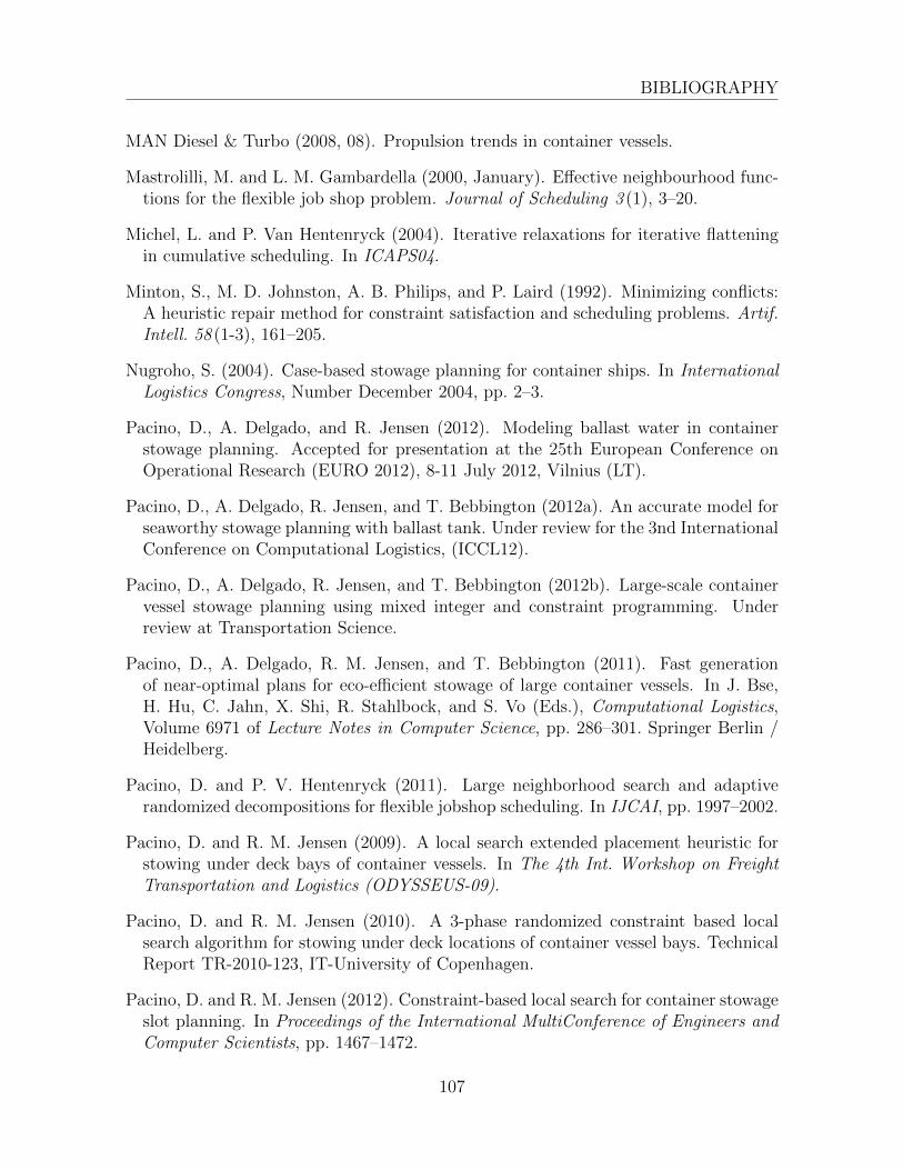
BIBLIOGRAPHY
MAN Diesel & Turbo (2008, 08). Propulsion trends in container vessels.
Mastrolilli, M. and L. M. Gambardella (2000, January). Effective neighbourhood func-tions for the flexible job shop problem. Journal of Scheduling 3 (1), 3–20.
Michel, L. and P. Van Hentenryck (2004). Iterative relaxations for iterative flatteningin cumulative scheduling. In ICAPS04.
Minton, S., M. D. Johnston, A. B. Philips, and P. Laird (1992). Minimizing conflicts:A heuristic repair method for constraint satisfaction and scheduling problems. Artif.Intell. 58 (1-3), 161–205.
Nugroho, S. (2004). Case-based stowage planning for container ships. In InternationalLogistics Congress, Number December 2004, pp. 2–3.
Pacino, D., A. Delgado, and R. Jensen (2012). Modeling ballast water in containerstowage planning. Accepted for presentation at the 25th European Conference onOperational Research (EURO 2012), 8-11 July 2012, Vilnius (LT).
Pacino, D., A. Delgado, R. Jensen, and T. Bebbington (2012a). An accurate model forseaworthy stowage planning with ballast tank. Under review for the 3nd InternationalConference on Computational Logistics, (ICCL12).
Pacino, D., A. Delgado, R. Jensen, and T. Bebbington (2012b). Large-scale containervessel stowage planning using mixed integer and constraint programming. Underreview at Transportation Science.
Pacino, D., A. Delgado, R. M. Jensen, and T. Bebbington (2011). Fast generationof near-optimal plans for eco-efficient stowage of large container vessels. In J. Bse,H. Hu, C. Jahn, X. Shi, R. Stahlbock, and S. Vo (Eds.), Computational Logistics,Volume 6971 of Lecture Notes in Computer Science, pp. 286–301. Springer Berlin /Heidelberg.
Pacino, D. and P. V. Hentenryck (2011). Large neighborhood search and adaptiverandomized decompositions for flexible jobshop scheduling. In IJCAI, pp. 1997–2002.
Pacino, D. and R. M. Jensen (2009). A local search extended placement heuristic forstowing under deck bays of container vessels. In The 4th Int. Workshop on FreightTransportation and Logistics (ODYSSEUS-09).
Pacino, D. and R. M. Jensen (2010). A 3-phase randomized constraint based localsearch algorithm for stowing under deck locations of container vessel bays. TechnicalReport TR-2010-123, IT-University of Copenhagen.
Pacino, D. and R. M. Jensen (2012). Constraint-based local search for container stowageslot planning. In Proceedings of the International MultiConference of Engineers andComputer Scientists, pp. 1467–1472.
107

BIBLIOGRAPHY
Pacino, D., K. Tierney, and R. M. Jensen (2012). Np-hard components of containervessel stowage planning. To be submitted to OR Letters.
Pezzella, F., G. MORGANTI, and G. CIASCHETTI (2008, October). A genetic al-gorithm for the Flexible Job-shop Scheduling Problem. Computers & OperationsResearch 35 (10), 3202–3212.
Sciomachen, A. and A. Tanfani (2003). The master bay plan problem: a solutionmethod based on its connection to the three-dimensional bin packing problem. IMAJournal of Management Mathematics 14, 251–269.
Scott, D. and D. Chen (1978). A loading model for a container ship. Technical report,Matson Navigation Company, Los Angeles.
Shields, J. J. (1984). Container stowage: A computer aided pre-planning system. Ma-rine Technology 21 (4).
Steenken, D., S. Voss, and R. Stahlbock (2004). Container terminal operation andoperations research - a classification and literature review. OR Spectrum 26, 3–49.
Tupper, E. C. (2009). Introdution to Naval Architecture. Elsevier.
Vaessens, R. R. (1995). Generalized job shop scheduling : complexity and local search.doctoral thesis, Eindhoven University of Technology.
Wilson, I. and P. Roach (1999). Principles of combinatorial optimization applied tocontainer-ship stowage planning. Journal of Heuristics 5, 403–418.
Wilson, I., P. Roach, and J. Ware (2001). Container stowage pre-planning: using searchto generate solutions, a case study. Knowledge-Based Systems 14 (3), 137–145.
Wilson, I. D. (1997). The Application of Artificial Intelligence Techniques to the Deep-sea Container Stowage Problem. Ph. D. thesis, University of Glamorgan.
Wilson, I. D. and P. Roach (2000). Container stowage planning: A methodology for gen-erating computerised solutions. Journal of the Operational Research Society 51 (11),248–255.
Yanbin, L., W. Kangping, G. Dongwei, P. Wei, and Z. Chunguang (2008). Multi-agentera model based on belief solves multi-port container stowage problem. In Proceed-ings of the 2008 Seventh Mexican International Conference on Artificial Intelligence,MICAI ’08, Washington, DC, USA, pp. 287–292. IEEE Computer Society.
Yoke, M., H. Low, X. Xiao, F. Liu, S. Y. Huang, W. J. Hsu, and Z. Li (2009). Anautomated stowage planning system for large containerships. In In Proceedings ofthe 4th Virtual Int. Conference on Intelligent Production Machines and Systems.
108

BIBLIOGRAPHY
Zhang, W., Y. Lin, and Z. Ji (2005). Model and algorithm for container ship stowageplanning based on bin-packing problem. Journal of Marine Science and Applica-tion 4 (3).
109