Embed Size (px)
Citation preview
PAVOL JOZEF ŠAFAacuteRIK UNIVERSITY IN KOŠICE
FACULTY OF SCIENCE
DEPARTMENT OF PHYSICAL SCIENCES
MICHAL JAŠČUR
QUANTUM THEORY OF MAGNETISM
Academic textbooks
Košice 2013
QUANTUM THEORY OF MAGNETISM
copy 2013 doc RNDr Michal Jaščur CSc
Reviewers Prof RNDr Vladimiacuter Lisyacute DrSc
Prof RNDr Peter Kollaacuter CSc
Number of pages 65
Number of authorsʹ sheets 3
Electronic academic textbook for Faculty of Science on P J Šafaacuterik University in Košice
The author of this textbook is accountable for the professional level and language correctness
The language and arrangement of the manuscript have not been revised
Publisher Pavol Jozef Šafaacuterik University in Košice
Location httpwwwupjsskpracoviskauniverzitna-kniznicae-publikaciapf
Available 10 10 2013
Edition second
ISBN 978-80-8152-049-5
Contents
Preface 2
1 Many-Body Systems 711 Systems of Identical Particles 712 Heitler-London Theory of Direct Exchange 11
2 Bogolyubov Inequality and Its Applications 1921 General Remarks on Bogolyubov Inequality 1922 Mean-Field Theory of the Spin-12
Anisotropic Heisenberg Model 20221 General Formulation 20222 Thermodynamic Properties of the Heisenberg
Model 27
3 Spin-Wave Theory 3131 Bloch Spin-Wave Theory of Ferromagnets 3132 Holstein-Primakoff theory of ferromagnets 36
321 Internal Energy and Specific heat 42322 Magnetization and Critical Temperature 44
33 Holstein-Primakoff theory of antiferromagnets 45331 Ground-State Energy 49332 Sublattice Magnetization 51
3
Contents
4 Jordan-Wigner Transformation for the XY Model 55
4
Preface
Preface
This is a supporting text for the undergraduate students interested in quan-tum theory of magnetism The text represents an introduction to varioustheoretical approaches used in this field It is an open material in the sensethat it will be supported by appropriate problems to be solved by studentat seminars and also as a homework
The text consists of four chapters that form closed themes of the in-troductory quantum theory of magnetism In the first part we explain thequantum origin of the magnetism illustrating the appearance of the ex-change interaction for the case of hydrogen molecule The second chapter isdevoted to the application of the Bogolyubov inequality to the Heisenbergmodel and it represents the part which is usually missing in the textbooksof magnetism The third chapter deals with the standard spin wave-theoryincluding the Bloch and Holstein-Primakoff a approach Finally we discussthe application of the Jordan-Wigner transformation to one-dimensionalspin-12 XY model
The primary ambition of this supportive text is to explain diverse math-ematical methods and their applications in the quantum theory of mag-netism The text is written in the form which should be sufficient to de-velop the skills of the students up to the very high level In fact it isexpected that students following this course will able to make their ownoriginal applications of the methods presented in this book
The reading and understanding this text requires relevant knowledgesfrom the mathematics quantum and statistical mechanics and also fromthe theory of phase transitions It is also expected that students are familiarwith computational physics programming and numerical mathematics thatare necessary to solve the problems that will be included in the MOODLEeducational environment of the PJ Safarik University in Kosice
Finally one should note that the text is mathematically and physicallyrather advanced and its understanding assumes supplementary study of the
5
Preface
books listed in the list of references
Kosice September 2013 Michal Jascur
6
Chapter 1
Many-Body Systems
11 Systems of Identical Particles
Magnetism is a many-body phenomenon and its origin can only be explainedwithin the quantum physics In this part we will investigate some impor-tant properties of the wavefunctions of quantum systems consisting of manyidentical particles that are important to understand magnetic properties inthe solid state In general the Hamiltonian of the many-body system de-pends on the time coordinates and spin variables of all particles Howeverin this part we will mainly investigate the symmetry properties of the wave-function that are independent on the time and therefore we can excludethe time from our discussion For simplicity we neglect also spin-degrees offreedom
Let us consider a system of N identical particles described by the many-body Hamiltonian H(r1 r2 rN ) which remains unchanged with respectto the transposition of arbitrary two particles in the system This fact canbe mathematically expressed as
H(r1 r2 rj rk rN) = H(r1 r2 rk rj rN) (11)
7
11 Systems of Identical Particles
or
PjkH(r1 r2 rj rk rN) = H(r1 r2 rk rj rN)Pjk
(12)
The previous equation defines the transposition operator Pjk of the jth andkth particle Since a mutual interchange of arbitrary particles in the systemdoes not change its state then the total wavefunction of the system obeysthe following relation
PjkΨ(r1 r2 rj rk rN) = eiαΨ(r1 r2 rk rj rN)
(13)
and
P2jkΨ(r1 r2 rj rk rN t) = e2iαΨ(r1 r2 rj rk rN)
(14)
where the real parameter α apparently satisfies equation
e2iα = 1 or eiα = plusmn1 (15)
The last equation implies that the total wavefunction either remains thesame or changes its sign when two arbitrary particles are interchanged inthe system In the first case the total wave function is called as a symmetricfunction and in the later one as an anti-symmetric function The symme-try of the wavefunction of an ensemble of identical particles is exclusivelygiven by the type of particles and does not depend on external conditionsIn fact it has been found that all particles obeying the Pauli exclusionprinciple have the antisymmetric wavefunction and all other particles havethe symmetric wavefunction Unfortunately the direct theoretical proof ofthis statement is impossible for strongly interacting particles since in real
8
11 Systems of Identical Particles
many-body systems is not possible to calculate exactly the total wavefunc-tion On the other hand the situation becomes tractable for the case ofnon-interacting or weakly interacting particle Therefore we at first will in-vestigate the system of spinless non-interacting identical particles and thenwe clarify the role of the interaction and spin
In the case of noninteracting particles the total Hamiltonian of the sys-tem can be expressed as a sum of single-particle Hamiltonians ie
H =Nsumj
Hj (16)
where N denotes the number if particles It is also well known that thetotal wavefunction of non-interacting particles can be written as a productof the single-particle wavefunctions namely
Ψ(r1 r2 rj rk rN) =Nprodj=1
ϕnj(rj) (17)
where nj represents the set of all quantum numbers characterizing the rele-vant quantum state of the jth particle The single-particle functions ϕnj
(rj)are of course the solutions of the stationary Schrodinger equation
Hjϕnj(rj) = εnj
ϕnj(rj) (18)
Here εnjdenote the eigenvalues of the single-particle Hamiltonian Hj so
that the eigenvalue of the total Hamiltonian is given by En1n2nN=
sumj εnj
The symmetric wavefunction describing whole system can be written in theform
Ψ(r1 r2 rj rk rN) = AsumP
ϕn1(r1)ϕn2(r2) ϕnN(rN) (19)
9
12 Heitler-London Theory of Direct Exchange
where A denotes the normalization constant and summation is performedover all possible permutation of the particles Similarly for the antisymmet-ric case we obtain the form
Ψ(r1 r2 rj rk rN) =1radicN
∣∣∣∣∣∣∣∣∣ϕn1(r1) ϕn1(r2) ϕn1(rN)ϕn2(r1) ϕn2(r2) ϕn2(rN)
ϕnN(r1) ϕnN
(r2) ϕnN(rN)
∣∣∣∣∣∣∣∣∣(110)
which is usually called as the Slater determinant It is clear that inter-changing of two particles in the system corresponds to the interchange ofrelevant rows in the determinant (110) which naturally leads to the signchange of the wavefunction Moreover if two or more particles occupy thesame state then two or more rows in the determinant (110) are equal andconsequently the resulting wavefunction is equal to zero in agreement withthe Pauli exclusion principle
Until now we have considered a simplified system of non-interacting par-ticles and we have completely neglected spin degrees of freedom Howeverthe situation in realistic experimental systems is much more complicatedsince each particle has a spin and moreover the interactions between parti-cles often also substantially influence the behavior of the system Howeverif we assume the case of weak interactions and if we neglect the spin-orbitinteractions then the main findings discussed above remain valid and more-over the existence of the exchange interaction can be clearly demonstratedInstead of developing an abstract and general theory for such a case itis much more useful to study a typical realistic example of the hydrogenmolecule which illustrates principal physical mechanisms leading to theappearance of magnetism
10
12 Heitler-London Theory of Direct Exchange
12 Heitler-London Theory of Direct Exchange
In the previous part we have found that the total wavefunction of themany-electron system must be anti-symmetric In this subsection we willdemonstrate that the use of anti-symmetric wave functions leads to thepurely quantum contribution to the energy of the system which is calledthe exchange energy In fact this energy initiates a certain ordering ofthe spins ie it may lead to the magnetic order in the system A similareffect we also obtain using the single-product wavefunctions if we explicitlyinclude the exchange-interaction term into Hamiltonian This effect wasindependently found by Heisenberg and Dirac in 1926 and it represent themodern quantum-mechanical basis for understanding magnetic propertiesin many real systems
a b
2
1
r
rrab
r r
ra
a
1
2 2b
21
1b
Figure 11 Schematic geometry of the H2 molecule The larger circles denotethe protons and the smaller ones represent two electrons The relevant distancesbetween different pairs of particles are denoted as rij where i j = a b 1 2
We start our analysis with one of the simplest possible system namely
11
12 Heitler-London Theory of Direct Exchange
H2 molecule In the hydrogen molecule two electrons interact with eachother and with the nuclei of the atoms The situation is schematicallydepicted in Fig11 and considering this geometry we can write the Hamil-tonian of the H2 molecule in the form
H = H1 + H2 + W + HLS (111)
where
H1 = minus ~2
2m∆1 minus
e20ra1
(112)
H2 = minus ~2
2m∆2 minus
e20rb2
(113)
W =e20rab
+e20r12
minus e20rb1
minus e20ra2
(114)
and we have used the abbreviation e0 = e(4πε0) The terms H1 and H2 in(111) describe the situation when the two hydrogen atoms are isolated Theoperator W describes the interaction between two cores electrons as wellas between electrons and relevant nuclei Finally the last term representsthe spin-orbit interaction which is assumed to be small so that we canseparate the orbital and spin degrees of freedom To solve the problem of thehydrogen molecule we apply the first-order perturbation theory neglectingthe spin-orbit coupling and taking the term W as a small perturbationAs it is usual in the perturbation theory we at first solve the unperturbedproblem ie the system of two non-interacting hydrogen atoms Thus wehave to solve the Schrodinger equation
(H1 + H2)Ψ = U0Ψ (115)
12
12 Heitler-London Theory of Direct Exchange
As we already have noted above we will assume that the total wave functioncan be written as a product of the orbital and spin functions ie Ψ =φ(r1 r2)χ(s
z1 s
z2) Another very important point to be emphasized here
is that our simplified Hamiltonian does not explicitly depend on the spinvariables Consequently we can at first evaluate only the problem withorbital functions and at the end of the calculation we can multiply theresult by an appropriate spin function to ensure the anti-symmetry of thetotal wavefunction In order to express this situation mathematically weintroduce the following notations
bull ϕα(ri)where α = a b i = 1 2 represents the orbital wave func-tion of the isolated hydrogen atom when the ith electron is localizedclosely to the αth nucleus
bull ξγ(i)where γ =uarr darr i = 1 2 is the spin function describing thespin up or spin down of the ith electron
Now let us proceed with the discussion of the orbital functions of the systemdescribed by Eq(115) Since the orbital functions ϕα(ri) are eigenfunctionsof the relevant one-atom Schrodinger equation with the same eigenvalueE0 = minus1355 eV it is clear that the ground state of the two noninteractinghydrogen atoms has the energy U0 = 2E0 and it is doubly degeneratedThis is so-called exchange degeneracy and two wavefunctions correspondingto this U0 can be expressed as φ1(r1 r2) = ϕa(r1)ϕb(r2) and φ2(r1 r2) =ϕa(r2)ϕb(r1)
If we include into Hamiltonian also the interaction term W then the sit-uation becomes much more complex and the eigenfunctions and eigenvaluescannot be found exactly In the spirit of the perturbation theory we willassume that the wavefunction of the interacting system can be expressed inthe form
φ(r1 r2) = c1φ1(r1 r2) + c2φ2(r1 r2)
= c1ϕa(r1)ϕb(r2) + c2ϕa(r2)ϕb(r1) (116)
13
12 Heitler-London Theory of Direct Exchange
where c1 and c2 are the constant that will be determined later The systemis now described by the following Schrodinger equation(H1 + H2 + W
)[c1φ1(r1 r2) + c2φ2(r1 r2
]= E
[c1φ1(r1 r2) + c2φ2(r1 r2)
](117)
Multiplying the previous equation by φlowast1(r1 r2) and integrating over the
space one obtains
2c1E0 + 2c2E0
intintφlowast1(r1 r2)φ2(r1 r2)dV1dV2
+ 2c1
intintφlowast1(r1 r2)Wφ1(r1 r2)dV1dV2 + c2
intintφlowast1(r1 r2)Wφ2(r1 r2)dV1dV2
= c1E + c2E
intintφlowast1(r1 r2)φ2(r1 r2)dV1dV2 (118)
Similarly by multiplying Eq(117) by φlowast2(r1 r2) and integrating over the
space one finds
c1E0
intintφlowast2(r1 r2)φ1(r1 r2)dV1dV2 + c1
intintφlowast2(r1 r2)Wφ1(r1 r2)dV1dV2
+ 2c2E0 + c2
intintφlowast2(r1 r2)Wφ2(r1 r2)dV1dV2
= c1E
intintφlowast2(r1 r2)φ1(r1 r2)dV1dV2 + c2E (119)
Here one should notice that in deriving Eqs(118) and (119) we have usednormalization conditions for φ1 and φ2
In order to express two previous equations in an abbreviated form oneintroduces the following quantities
1 The overlap integral
S0 =
intϕlowasta(ri)ϕb(ri)dVi i = 1 2 (120)
14
12 Heitler-London Theory of Direct Exchange
2 The Coulomb integral
K =
intintφlowast1(r1 r2)Wφ1(r1 r2)dV1dV2 =
intintφlowast2(r1 r2)Wφ2(r1 r2)dV1dV2
(121)
3 The exchange integral
A =
intintφlowast1(r1 r2)Wφ2(r1 r2)dV1dV2 =
intintφlowast2(r1 r2)Wφ1(r1 r2)dV1dV2
(122)
Applying this notation we rewrite Eqs(118) and (119) in the form
c1(2E0 +K minus E) + c2(2E0S20 + Aminus ES2
0) = 0
c1(2E0S20 + Aminus ES2
0) + c2(2E0 +K minus E) = 0 (123)
This is a homogeneous set of equations which determines unknown coeffi-cients c1 and c2 Of course we search for non-trivial solutions that can benaturally determined from the equation∣∣∣∣ 2E0 +K minus E 2E0S
20 + Aminus ES2
0
2E0S20 + Aminus ES2
0 2E0 +K minus E
∣∣∣∣ = 0 (124)
From this equation we easily find two possible solutions for the energy Eand the coefficients ci namely
Ea = 2E0 +K minus A
1minus S20
c1 = minusc2 (125)
and
Es = 2E0 +K + A
1 + S20
c1 = c2 (126)
15
12 Heitler-London Theory of Direct Exchange
Finally from the normalization condition of the total wavefunction oneobtains
1 =
int intφlowast(r1 r2)φ(r1 r2)dV1dV2
= 2|c1|2(1∓ S2) (127)
or
c1 =1radic
2(1∓ S20) (128)
where the minus and + sign corresponds to Ea and Es respectively Using(128) we can express the orbital part of the total wavefunctions as
φ(r1 r2) =1radic
2(1minus S20)
[ϕa(r1)ϕb(r2)minus ϕa(r2)ϕb(r1)
](129)
which is clearly the anti-symmetric expression and it corresponds to EaSimilarly the symmetric orbital function which corresponds to Es is givenby
φ(r1 r2) =1radic
2(1 + S20)
[ϕa(r1)ϕb(r2) + ϕa(r2)ϕb(r1)
] (130)
Finally we also can account for the spins of the electrons and to con-struct the following anti-symmetric wavefunctions
Ψ =1radic
2(1minus S20)
∣∣∣∣ ϕa(r1) ϕa(r2)ϕb(r1) ϕb(r2)
∣∣∣∣ ξuarr(1)ξuarr(2) S = 1 Sz = 1 (131)
Ψ =1radic
2(1minus S20)
∣∣∣∣ ϕa(r1) ϕa(r2)ϕb(r1) ϕb(r2)
∣∣∣∣ ξdarr(1)ξdarr(2) S = 1 Sz = 0 (132)
16
12 Heitler-London Theory of Direct Exchange
Ψ =1radic
2(1minus S20)
∣∣∣∣ ϕa(r1) ϕa(r2)ϕb(r1) ϕb(r2)
∣∣∣∣ 1radic2[ξuarr(1)ξdarr(2) + ξdarr(1)ξuarr(2)]
S = 1 Sz = minus1 (133)
and
Ψ =1radic
2(1 + S20)
[ϕa(r1)ϕb(r2) + ϕb(r1)ϕa(r2)
] 1radic2
∣∣∣∣ ξuarr(1) ξuarr(2)ξdarr(1) ξuarr(2)
∣∣∣∣S = 0 Sz = 0 (134)
Here the wavefunctions (131)-(133) form a triplet (threefold degeneratestate) with the energy Ea the total spin S = 1 and the total zth componentSz = plusmn1 0 Similarly the wavefunction (134) describes a singlet state withenergy Es the total spin S = 0 and Sz = 0 Of course both the triplet andsinglet states can be the ground state of the system depending on the signof the exchange integral In order to prove this statement we calculate theenergy difference between Ea and Es ie
∆E = Ea minus Es =2(KS2
0 minus A)
1minus S40
asymp minus2A (135)
where we have neglected the overlap integral which very small in comparisonwith other terms in the expression It is clear from the previous equationthat for A gt 0 the ground state of the system will be represented by thetriplet state with parallel alignment of spins and for A lt 0 the singlet statewith anti-parallel orientation of the spins Of course the parallel (anti-parallel) spin orientation implies also parallel (anti-parallel) alignment of themagnetic moments which is crucial for the observation of the ferromagneticor antiferromagnetic ordering in the real systems
The situation in the hydrogen molecule of course differs from the realsituation in ionic crystal in many respects For example the electrons in
17
12 Heitler-London Theory of Direct Exchange
the hydrogen molecule occupy 1s orbitals while in the ionic crystals theunpaired localized electrons usually occupy d or f orbitals In fact thecalculation of the exchange integral using 3d orbital functions leads to thepositive value of the A Therefore the direct exchange interactions leadsto the ferromagnetic ordering in such systems Later it was discovered byAnderson that the antiferromagnetic ordering is caused by so-called indi-rect exchange interaction via a non-magnetic bridging atom The situationin real materials is usually much more complicated and other mechanismsuch as the Dzyaloshinkii-Moriya or Ruderman-Kittel-Kasuya-Yosida inter-actions can play an important role
Although the calculation performed for the hydrogen molecule does notreflect the complex situation of the real magnetic systems it is extremelyimportant from the methodological point of view In fact it is clear from ourcalculation that the parallel or anti-parallel alignment of the magnetic mo-ments appears due to new contribution to the energy of the system whichoriginates from the indistinguishability of quantum particles The othermechanisms leading to the macroscopic magnetism have also quantum na-ture and cannot be included into the classical theory
Thus we can conclude that the physical origin of magnetism can becorrectly understood and described only within the quantum theory
18
Chapter 2
Bogolyubov Inequality and ItsApplications
21 General Remarks on Bogolyubov Inequal-
ity
The Bogolyubov inequality for the Gibbs free energy G of an interactingmany-body system described by the Hamiltonian H is usually written inthe form
G le G0 + ⟨H minus H0⟩0 = ϕ(λx λy λz ) (21)
In this equation the so-called trial Hamiltonian H0 = H0(λx λy λz )depends on some variational parameters λi that are naturally determinedin the process of calculation and the symbol ⟨ ⟩0 stands for the usualensemble average calculated with the trial Hamiltonian Finally G0 denotesthe Gibbs free energy of the trial system defined by
G0 = G0(λx λy λz ) = minus 1
βlnZ0 (22)
19
22 Mean-Field Theory of Anisotropic Heisenberg Model
where β = 1kBT and the the partition function Z0 is given by
Z0 = Tr eminusβH0 (23)
In general there is a remarkable freedom in defining the trial Hamilto-nian In fact the only limitations to be taken into account follow from thetwo obvious requirements
1 The trial Hamiltonian should naturally represent a simplified physicalmodel of the real system
2 The expression of G0 must be calculated exactly in order to obtain aclosed-form formula for the rhs of Eqs(21)
22 Mean-Field Theory of the Spin-12
Anisotropic Heisenberg Model
221 General Formulation
The accurate theoretical analysis of the Heisenberg model is extremely harddue to interaction terms in the Hamiltonian including non-commutative spinoperators Probably the simplest analytic theory applicable to the modelis the standard mean-field approach Although the mean-field theory canmathematically be formulated in many different ways we will develop in thistext an approach based on the Bogolyubov inequality for the free energy ofthe system The main advantage of this formulation is its completeness (wecan derive analytic formulas for all thermodynamic quantities of interest)and a possibility of further generalizations for example an extension to theOguchi approximation
20
22 Mean-Field Theory of Anisotropic Heisenberg Model
In this part we will study the spin-12 anisotropic Heisenberg model ona crystal lattice described by the Hamiltonian
H = minussumij
(JxSxi S
xj + JyS
yi S
yj + JzS
zi S
zj )minus gmicroB
sumi
(HxSxi +HyS
yi +HzS
zi )
(24)where g is the Lande factor microB is the Bohr magneton Jα and Hα α =x y z denote the spatial components of the exchange interaction and exter-nal magnetic field respectively One should note here that Jα is assumedto be positive for the ferromagnetic systems and negative for the antifer-romagnetic ones Moreover it is well-known that the absolute value ofexchange integrals very rapidly decreases with the distance thus we canrestrict the summation in the first term of (24) to the nearest-neighboringpairs of atoms on the lattice Finally the spatial components of the spin-12operators are given by
Sxk =
1
2
(0 11 0
)k
Syk =
1
2
(0 minusii 0
)k
Szk =
1
2
(1 00 minus1
)k
(25)
To proceed further we choose the trial Hamiltonian in the form
H0 = minusNsumk
(λxS
xk + λyS
yk + λzS
zk
) (26)
where N denotes the total number of the lattice sites and λi are variationalparameters to be determined be minimizing of the rhs of the Bogolyubovinequality After substituting (25) into (26) we can apparently rewriteprevious equation as follows
H0 =Nsumk=1
H0k (27)
21
22 Mean-Field Theory of Anisotropic Heisenberg Model
where the site Hamiltonian H0k is given by
H0k = minus1
2
(λz λx minus iλy
λx + iλy minusλz
)k
(28)
In order to evaluate the terms entering the Bogolyubov inequality we atfirst have to calculate the partition function Z0 Taking into account thecommutation relation [H0k H0ℓ] = 0 for k = ℓ we obtain the followingexpression
Z0 = Tr exp(minusβ
Nsumk=1
H0k
)=
Nprodk=1
Trk exp(minusβH0k
) (29)
where Trk denotes the trace of the relevant operator related to kth latticesite Now after setting Eq(28) into (29) one obtains
Z0 =Nprodk=1
Trk exp
(β2λz
β2(λx minus iλy)
β2(λx + iλy) minusβ
2λz
)k
=
[Trk exp
(β2λz
β2(λx minus iλy)
β2(λx + iλy) minusβ
2λz
)k
]N
(210)
The crucial point for further calculation is the evaluation of exponentialfunction in previous equation Let us note that in performing this task wewill not follow the usual approach based on the diagonalization of modifiedmatrix (28) entering the argument of exponential Instead we will performall calculations in the real space by applying the following matrix form ofthe Cauchy integral formula
eminusβH0k =1
2πi
∮C
ezdz
zI minus (minusβH0k) (211)
22
22 Mean-Field Theory of Anisotropic Heisenberg Model
After a straightforward calculation we obtain
eminusβH0k =
(h11 h12
h21 h22
)(212)
with
h11 = cosh
(β
2Λ
)+
λz
Λsinh
(β
2Λ
)(213)
h12 =λx minus iλy
Λsinh
(β
2Λ
)(214)
h21 =λx + iλy
Λsinh
(β
2Λ
)(215)
h22 = cosh
(β
2Λ
)minus λz
Λsinh
(β
2Λ
) (216)
where we have introduced the parameter
Λ =radicλ2x + λ2
y + λ2z (217)
Using previous equations we easily obtain the following expressions for Z0
and G0
Z0 =
[2 cosh
(β
2Λ
)]N(218)
G0 = minusN
βln
[2 cosh
(β2Λ
)] (219)
23
22 Mean-Field Theory of Anisotropic Heisenberg Model
To obtain the complete expression for ϕ(λx λy λz ) we have to eval-
uate the terms ⟨H⟩0 and ⟨H0⟩0 that can be expressed as
⟨H⟩0 = minusNq
2
(Jx⟨Sx
i Sxj ⟩0 + Jy⟨Sy
i Syj ⟩0 + Jz⟨Sz
i Szj ⟩0
)minus N
(hx⟨Sx
j ⟩0 + hy⟨Syj ⟩0 + hz⟨Sz
j ⟩0) (220)
where q denotes the coordination number of the lattice and hα = gmicroBHα(α = x y z) Similarly we have
⟨H0⟩0 = minusN(λx⟨Sx
j ⟩0 + λy⟨Syj ⟩0 + λz⟨Sz
j ⟩0) (221)
The ensemble averages of ⟨Sαj ⟩0 entering two previous equations can be
expressed in the form
⟨Sαj ⟩0 =
1
Z0
TrSαj e
minusβH0
=TrjS
αj exp
(minusβH0j
)prodNminus1k =j Trk exp
(minusβH0k
)Trj exp
(minusβH0j
)prodNminus1k =j Trk exp
(minusβH0k
) (222)
which can be simplified as follows
⟨Sαj ⟩0 =
TrjSαj exp
(minusβH0j
)Trj exp
(minusβH0j
) (223)
Similarly one easily finds that
⟨Sαi S
αj ⟩0 =
TriSαi exp
(minusβH0i
)Tri exp
(minusβH0i
) TrjSαj exp
(minusβH0j
)Trj exp
(minusβH0j
) =(⟨Sα
j ⟩0)2
(224)
24
22 Mean-Field Theory of Anisotropic Heisenberg Model
In order to complete our calculation we substitute Eqs (212)-(216) intoEq (223) and then we evaluate the trace of relevant matrices In this waywe obtain the following equation
⟨Sαj ⟩0 =
λα
2Λtanh
(β
2Λ
) (225)
and
⟨Sαi S
αj ⟩0 =
(λα
2Λ
)2
tanh2
(β
2Λ
) (226)
After introducing notation ⟨Sαj ⟩0 = mα α = x y z we can rewrite the rhs
of the Bogolyubov inequality in the form
ϕ(λx λy λz) = minusN
βln(2 cosh
β
2Λ)minus Nq
2
(Jxm
2x + Jym
2y + Jzm
2z
)+ N
[(λx minus hx)mx + (λy minus hy)my + (λz minus hz)mz
] (227)
Since the quantity ϕ represents an upper bound for the exact Gibbs freeenergy of the system then the best possible approximation (with the trialHamiltonian H0) corresponds for those values of λx λy λz that minimizeϕ(λx λy λz) Relevant values of λx λy λz are obviously determined fromthe equations
partϕ
partλx
= 0partϕ
partλy
= 0partϕ
partλz
= 0 (228)
The above conditions lead to three independent equations that can berewritten in the following simple matrix form
partmx
partλx
partmy
partλx
partmz
partλxpartmx
partλy
partmy
partλy
partmz
partλy
partmx
partλz
partmy
partλz
partmz
partλz
λx minus qJxmx minus hx
λy minus qJymy minus hy
λz minus qJzmz minus hz
= 0 (229)
25
22 Mean-Field Theory of Anisotropic Heisenberg Model
Since the first matrix in (229) is in general non-zero then the only possiblesolution of this equation is given by
λx = qJxmx + hx λy = qJymy + hy λz = qJzmz + hz (230)
and the cooresponding equilibrium Gibbs free energy can be after a smallmanipulation expressed in the form
G = minusN
βln2 cosh
(βhef
2
)+
Nq
2
(Jxm
2x + Jym
2y + Jzm
2z
) (231)
where we have denoted
hef =radic
(qJxmx + hx)2 + (qJymy + hy)2 + (qJzmz + hz)2 (232)
Having obtained the last equation we are able to identify the physicalmeaning of the parameters mxmymx and consequently also the meaningof variational parameters λx λy λz
For this purpose we at first recall that the spatial component of thetotal magnetization Mα is defined as
Mα = minus(
partGpartHα
)β
= minusgmicroB
(partGparthα
)β
(233)
After a straightforward calculation we obtain the following very simple ex-pressions
Mx
NgmicroB
= mx = ⟨Sxj ⟩0
My
NgmicroB
= my = ⟨Syj ⟩0
Mz
NgmicroB
= mz = ⟨Szj ⟩0
(234)
which clearly indicate that mα represents the spatial components of themagnetization Consequently the parameters λα have the meaning of ofthe molecular-field components acting on one atom in the lattice Thusour formulation is nothing but the standard mean-field theory The mainadvantage of our approach is that this formulation provides a close-form an-alytical expression for the Gibbs free energy which is of principal importancefor finding stability conditions of various physical quantities
26
22 Mean-Field Theory of Anisotropic Heisenberg Model
222 Thermodynamic Properties of the HeisenbergModel
Now let us proceed with the calculation of several interesting physical quan-tities for the system under investigation Using Eqs (222) (230) and(234) one simply obtains for the components of reduced magnetization aset of three coupled equations namely
mx =qJxmx + hx
2hef
tanh
(β
2hef
) (235)
my =qJymy + hy
2hef
tanh
(β
2hef
) (236)
mz =qJzmz + hz
2hef
tanh
(β
2hef
) (237)
where we have denotedIn order to investigate the long-range ordering the systems we set hx =
hy = hz = 0 and obtain
mx =Jxmx
2h0
tanh
(βq
2h0
) (238)
my =Jymy
2h0
tanh
(βq
2h0
) (239)
mz =Jzmz
2h0
tanh
(βq
2h0
) (240)
27
22 Mean-Field Theory of Anisotropic Heisenberg Model
with
h0 =radic(Jxmx)2 + (Jymy)2 + (Jzmz)2 (241)
These three nonlinear equations have always the trivial solution mx =my = mz = 0 corresponding to the disordered paramagnetic phase (DP)Moreover depending on the temperature and the values of exchange pa-rameters there also exist non-trivial solutions corresponding to ordered fer-romagnetic phase (OP) The stability of the relevant solutions is then de-termined by the minimum of the Gibbs free energy given by Eq(231) Nowwe briefly analyze possible trivial and non-trivial solutions of (238)-(240)for some particular cases of the exchange interactions
1 Ising model Jx = Jy = 0 Jz = J = 0
mx = my = 0 and mz =1
2tanh
(qβJ2
mz
)for T lt Tc
mx = my = mz = 0 for T gt Tc (242)
2 Isotropic XY model Jx = Jy = J = 0 Jz = 0
mz = 0my = mx and mx =1
2radic2tanh
(radic2qβJ
2mx
)for T lt Tc
mx = my = mz = 0 for T gt Tc (243)
3 Isotropic Heisenberg model Jx = Jy = Jz = 0
my = mx = mz and mz =1
2radic3tanh
(radic3qβJx2
mx
)for T lt Tc
mx = my = mz = 0 for T gt Tc (244)
28
22 Mean-Field Theory of Anisotropic Heisenberg Model
Here one should note that non-trivial results for isotropic XY and Heisen-berg model model represents valid solution for the models when the axis ofquantization is given by the equation y = x = t t isin R for the XY modeland y = x = z = t t isin R for the Heisenberg model On the other handif choose as a quantization axis for example the x axis then we obtain forboth models identical result as that for the Ising one Thus one can concludethat mean-field theory is not able to describe correctly quantum featuresof localized spin models In order to illustrate the numerical accuracy ofthe method we have compared in Fig 23 the temperature variation of themean-field magnetization with exact result on the square lattice with q = 4
00 05 10 15000
025
050q = 4
m
kBT J
Exact
MFT
Figure 21 Comparisom of the temperature dependence of magnetization forthe Ising model on a square lattice
The critical (or Curie) temperature is defined as a temperature at whichthe long-range order (or magnetization) vanishes In order to determine the
29
22 Mean-Field Theory of Anisotropic Heisenberg Model
Curie temperature we take into account that tanh(x) asymp x for x ltlt 1 andobtain an universal solution
Tc =qJα
4kB α = x y z (245)
which valid for all three cases mentioned above Of course the critical tem-perature should be different depending on the model considered Thus thepresent method is not able to distinguish specific features of the models aslong as concerns the critical behavior Moreover it is also clear that thetopology of the lattice is taken into account only through its coordinationnumber that is also weak point of the present method It is well knownthat this approach significantly fails for the low-dimensional systems nev-ertheless it gives rather good qualitative picture for the three-dimensionalsystems and therefore it is frequently used to obtain analytical results par-ticularly for complex systems
Finally one should note that calculations of other thermodynamic quan-tities is easy and straightforward since we have analytical solution for theGibbs free energy of the system from which other quantities are easily ob-tained
This calculation including numerical analysis and discussion is left forthe readers as an appropriate exercise
Let us conclude this part by noticing that the present approach can beextended to case of the the so-called Oguchi approximation which alreadyaccount much better for the quantum effects as well as for the spin-spincorrelations Possible extensions are rather involved and require lengthycalculations that are beyond the scope of the present book
30
Chapter 3
Spin-Wave Theory
31 Bloch Spin-Wave Theory of Ferromag-
nets
In this part we will discuss the concept of spin waves which enables to studythe some physical properties of magnetic systems at low temperatures Thistheory was originally introduced by F Bloch [1] and its main assumptionis that the ground state of the system is ordered and the excited states aredescribed as a collection of spin waves At low temperatures it is reasonableto expect the small amplitudes of the spin waves thus the interaction amongspin waves can be neglected We will consider in this part an isotropicHeisenberg model defined by the Hamiltonian
H = minusJsumij
SiSj minus gmicroBHsumi
Szi (31)
Here Si represents a vector spin-operator at the ith site of the lattice Thisoperator is naturally defined as Si = (Sx
i Syi S
zi ) where Sα
i (α = x y z)represent spatial components of the standard spin operators g is the Lande
31
31 Bloch Spin-Wave Theory of Ferromagnets
factor microB is the Bohr magneton and H denotes the external magnetic fieldwhich is applied along z axis J is the exchange integral which is assumedto be positive since we are going to investigate the ferromagnetic systems
Adopting the basic concept of lattice vibrations we can write the fol-lowing equation of motion of the spin Sℓ on the j th lattice point
dSℓ
dt=
i
~[H Sℓ] (32)
In what follows we will use the following commutation relations for spinoperators
[Sai S
bj ] = iεabcδijS
cj a b c = x y or z (33)
where εabc represents Levi-Civita tensor and δij is the Kronecker symbolNow substituting the Hamiltonian (31) into (32) and employing relations(33) one obtains
dSℓ
dt= minus1
~(Hℓ times Sℓ) (34)
where the local magnetic field Hℓ acting on the j th spin is given by
Hℓ =sumj
JjℓSj + gmicroBHe3 (35)
with e3 = (0 0 1) Using two previous equations one easily obtains thefollowing equations of motion of the x y and z components of the spinoperator
~dSx
ℓ
dt= minus
sumj
Jjℓ(Syj S
zℓ minus Sz
j Syℓ ) + gmicroBHSy
ℓ (36)
~dSy
ℓ
dt= minus
sumj
Jjℓ(Szj S
xℓ minus Sx
j Szℓ )minus gmicroBHSx
ℓ (37)
32
31 Bloch Spin-Wave Theory of Ferromagnets
~dSz
ℓ
dt= minus
sumj
Jjℓ(Sxj S
yℓ minus Sy
j Sxℓ ) (38)
If we restrict ourselves to the case of low-energy excitation then the compo-nents Sx
ℓ Syℓ can be regarded as small quantities of first order Consequently
the right-hand side of (38) is a small quantity of the second order whichcan be neglected and it follows from Eq (38) that the zth component be-comes a constant Moreover it is reasonable to put explicitly Sz
ℓ = S sincethe external magnetic field is assumed to be applied parallel to the zth axisUnder these assumptions Eqs (36) and (37) can be rewritten in the form
~dSx
ℓ
dt= minusS
sumj
Jjℓ(Syj minus Sy
ℓ ) + gmicroBHSyℓ (39)
~dSy
ℓ
dt= minusS
sumj
Jjℓ(Sxℓ minus Sx
j )minus gmicroBHSxℓ (310)
or alternatively
~dS+
ℓ
dt= minusiS
sumj
Jjℓ(S+ℓ minus S+
j )minus gmicroBHS+ℓ (311)
~dSminus
ℓ
dt= minusiS
sumj
Jjℓ(Sminusℓ minus Sminus
j )minus gmicroBHSminusℓ (312)
where we have introduced the spin-raising and spin-lowering operators
S+ℓ = Sx
ℓ + iSyℓ Sminus
ℓ = Sxℓ minus iSy
ℓ (313)
that obey the following commutation rules
[Szk S
+ℓ ] = S+
k δkℓ [Szk S
minusℓ ] = minusSminus
k δkℓ [S+k S
+ℓ ] = 2Sz
kδkℓ (314)
33
31 Bloch Spin-Wave Theory of Ferromagnets
The above relations are directly obtained with the help of well-known com-mutation relations of the spin operators (33)
To proceed further we now express the spin-raising and spin-loweringoperators with the help of the Fourier transform ie
S+q =
1radicN
sumj
eiqmiddotRj S+j Sminus
q =1radicN
sumj
eminusiqmiddotRj Sminusj (315)
S+j =
1radicN
sumq
eminusiqmiddotRj Sq Sminusj =
1radicN
sumq
eiqmiddotRj Sq (316)
Substituting Eq(316) into Eq(312) and applying the following relationsumℓ
eminusi(q1minusq2)middotRℓ = Nδq1q2 (317)
one gets equation
minusi~dSminus
q
dt=
[Ssumℓ
Jjℓ(1minus eminusiqmiddot(RjminusRℓ)) + gmicroBH]Sminusq (318)
If we now introduce a real quantity
J(q) =sumj
J(Rj)eminusiqmiddotRj (319)
then we rewrite (318) as
minusi~dSminus
q
dt=
S[J(0)minus J(q)
]+ gmicroBH
Sminusq (320)
It is straightforward to obtain the solution of this equation in the form
Sq = δSqei(ωqt+α) (321)
34
31 Bloch Spin-Wave Theory of Ferromagnets
where the eigenfrequencies of the spin waves are given by
~ωq = S[J(0)minus J(q)
]+ gmicroBH (322)
One should notice here that in the limit of small q we obtain ~ωq asymp q2Now using Eq(321) we can express the spin operators in the real space
as follows
Sminusj =
1radicNδSqe
i(qmiddotRj+ωqt+α) (323)
Sxj =
1radicNδSq cos
[i(q middotRj + ωqt+ α)
](324)
and
Syj = minus 1radic
NδSq sin
[i(q middotRj + ωqt+ α)
] (325)
Finally it is straightforward to prove that the energy difference betweenan excited state and ground state is given by
Eq minus E0 = ~ωq (326)
where ~ωq represents the excitation energy of the spin wave with the wavevec-tor q The proof of the last statement is left as an appropriate exercise forreaders
35
32 Holstein-Primakoff theory of ferromagnets
32 Holstein-Primakoff theory of ferromag-
nets
The Blochrsquos spin-wave theory discussed in previous chapter represents a verysimple approach in which we completely neglect the interaction among spinwaves This deficiency can be eliminated using an alternative formulationbased on magnon variables (or creation-annihilation operators) developedby Holstein and Primakoff [2] In this part we apply The Holstein-Primakofftheory to case of an anisotropic quantum Heisenberg model described bythe Hamiltonian
H = minusJsumij
(Sxi S
xj + Sy
i Syj + Sz
i Szj )minus gmicroBH
sumi
Szi (327)
The meaning of all symbols in previous Eq (327) is the same as in previoustext
In order to apply a spin-wave picture to analyze magnetic properties ofthe model under investigation one has to perform three subsequent math-ematical transformation At first we express the components of the spinoperators trough spin-lowering and spin raising operators then we intro-duce so-called creation and annihilation operators and finally we performa Fourier transform of the relevant all creation and annihilation operatorsentering the Hamiltonian The eigenvalues of the final Hamiltonian then en-able to determine relevant physical quantities applying standard relationsof statistical mechanics For further manipulations it is more convenient torewrite (327) as follows
H = minusJsumℓδ
(Sxℓ S
xℓ+δ + Sy
ℓ Syℓ+δ + Sz
ℓ Szℓ+δ)minus gmicroBH
sumℓ
Szℓ (328)
where ℓ labels the lattice sites and δ denotes nearest neighbors of the relevantsite and we assume that J gt 0 The integrals of motion for Hamiltonian
36
32 Holstein-Primakoff theory of ferromagnets
(328) are the total z th component Sz =sum
k Szk and the total spin of the
systemThe ground state of the system is ordered and for H gt 0 the magnetic
moment is paralell to the z axis If we consider the lattice consisting of Natoms with spin S then the ground-state vector in the spin basis reads |0⟩= |NSNS⟩ Of course we work in a real space basis in which the spinoperators Sz
ℓ are diagonal We recall that the eigenvalues MS = minusS minusS +1 S and eigenvectors |MS⟩ℓ of the operator Sz
ℓ satisfy the followingequation
Szℓ |MS⟩ℓ = MS|MS⟩ℓ (329)
Now applying operators (313) to the eigenvectors |MS⟩ℓ one obtains
S+ℓ |MS⟩ℓ =
radic(S minusMS)(S minusMS minus 1)|MS + 1⟩ℓ (330)
and
Sminusℓ |MS⟩ℓ =
radic(S +MS)(S minusMS minus 1)|MS minus 1⟩ℓ (331)
In addition to the spin-raising and spin-lowering operators we will alsouse in our analysis the operator describing a deviation of the zth spin-component from its maximum value namely
nℓ = S minus Szℓ (332)
The eigenvalues of this operator are integers nl = 0 1 2 2S (or nl =S minusMS) thus we can rewrite Eqs(330) in the form
S+ℓ |nℓ⟩ℓ =
radic2S
radic1minus (nℓ minus 1)
2S
radicnℓ|nℓ minus 1⟩ℓ (333)
Le us note that performing a similar procedure is also possible for Eq(331)and it will be used later
37
32 Holstein-Primakoff theory of ferromagnets
Now with the help of (313) we can rewrite the Hamiltonian (328) inthe form
H = minusJsumℓδ
[12(S+
ℓ Sminusℓ+δ + Sminus
ℓ S+ℓ+δ) + Sz
ℓ Szℓ+δ
]minus gmicroBH
sumℓ
Szℓ (334)
which is suitable for introducing the Holstein-Primakoff magnon represen-tation In order to define the relevant transformation we at first introducethe standard creation and annihilation operators that are defined as
adaggerℓΨnℓ=
radicnℓ + 1Ψnℓ+1 aℓΨnℓ
=radicnℓΨnℓminus1 (335)
The central idea of the Holstein-Primakoff approach is based on the intro-duction of the following transformation
S+ℓ = (2S)12
(1minus adaggerℓaℓ
2S
)12
aℓ (336)
Sminusℓ = (2S)12adaggerℓ
(1minus adaggerℓaℓ
2S
)12
(337)
Szℓ = S minus adaggerℓaℓ (338)
As already noted above the eigenvalues of adaggerℓaℓ are arbitrary integers whilethat of nℓ are limited to the range 0 le nℓ le 2S Fortunately this discrep-ancy does not play any important role in the calculation since the transitionfrom the state with nℓ le 2S to states with nℓ gt 2S never occur eg
Sminusℓ Ψ2S = (2S)12(2S + 1)12
(1minus 2S
2S
)12
Ψ2S+1 = 0 (339)
Now we transform the operators aℓ adaggerℓ from the real space to the reciprocal
space by the following Fourier tansform
aℓ =1radicN
sumq
eminusiqmiddotRℓbq (340)
38
32 Holstein-Primakoff theory of ferromagnets
adaggerℓ =1radicN
sumq
eiqmiddotRℓbdaggerq (341)
where N denotes the total number of atoms q represents a vector of thereciprocal space and Rℓ represents a vector specifying the position of ℓthatom in the lattice
The magnon-annihilation and magnon-creation operators are given by
bq =1radicN
sumℓ
eiqmiddotRℓaℓ (342)
bdaggerq =1radicN
sumℓ
eminusiqmiddotRℓadaggerℓ (343)
and they obey the usual magnon commutation relations
[bq1 bdaggerq2] = δq1q2 [bq1 bq2 ] = [bdaggerq1
bdaggerq2] = 0 (344)
It is useful to note here that the operator bdaggerq creates a magnon with thewave vector q and the operator bq annihilates it Moreover it follows fromthe transformation (340) and (341) that any change of the spin state atarbitrary lattice site is described as a superposition of an infinite number ofthe spin waves
At this stage it is clear that further exact treatment of the problem isimpossible due to the complexity of applied transformations The progressis however still possible if we restrict ourselves to the case when the numberof excited states is small in comparison with 2S Under this assumptionwe can neglect the higher order terms in expansion of the square root andrewrite Eqs (336) and (337) in the form
S+ℓ = (2S)12
(1minus adaggerℓaℓ
4S
)aℓ + (345)
39
32 Holstein-Primakoff theory of ferromagnets
Sminusℓ = (2S)12adaggerℓ
(1minus adaggerℓaℓ
4S
)+ (346)
Finally substituting (340) and (341) into previous equation one obtains
S+ℓ =
(2S
N
)12[sumq1
eminusiq1middotRℓbq1 minus1
4SN
sumq1q2q3
ei(q1minusq2minusq3)middotRℓbdaggerq1bq2bq3 +
](347)
Sminusℓ =
(2S
N
)12[sumq1
eiq1middotRℓbdaggerq1minus 1
4SN
sumq1q2q3
ei(q1+q2minusq3)middotRℓbdaggerq1bdaggerq2
bq3 +
](348)
Similarly the operator Szℓ is given by
Szℓ = S minus 1
N
sumq1q2
ei(q1minusq2)middotRℓbdaggerq1bq2 (349)
If we assume that each lattice site has z nearest neighbors then we canspecify their positions on the lattice by introducing the vector
δ = Rℓ+δ minusRℓ (350)
Substituting (347)-(350) into Eq(334) and performing a rearrange-ment of the terms one can rewrite the Hamiltonian as
H = minusJNzS2 minus gmicroBNHS + H0 + H1 (351)
where H0 is a bilinear form in the magnon variables and it is given by
H0 = minus JS
N
sumℓδ
sumq1q2
[eminusi(q1minusq2)middotRℓeiq2middotδbq1b
daggerq2
+ ei(q1minusq2)middotRℓeminusiq2middotδbdaggerq1bq2
]+
JS
N
sumℓδ
sumq1q2
[ei(q1minusq2)middotRℓbq1b
daggerq2
+ eminusi(q1minusq2)middotRℓei(q1minusq2)middotδbdaggerq1bq2
]+
gmicroBH
N
sumℓq1q2
ei(q1minusq2)middotRℓbdaggerq1bq2 (352)
40
32 Holstein-Primakoff theory of ferromagnets
The term H1 includes higher-order terms and for the sake of simplicity willbe neglected Now taking into account the relation (317) and performingthe summation over ℓ and q2 we can simplify Eq(352) as follows
H0 = minusJzSsumq
(γqbqbdaggerq + γminusqb
daggerqbq minus 2bdaggerqbq) + gmicroBH
sumq
bdaggerqbq (353)
where
γq =1
z
sumδ
eiqmiddotδ (354)
and the summation in (354) runs over all nearest neighbors For furthermanipulation it useful noticing that
sumq γq = 0 and moreover for the crys-
tals with the symmetry center we have γq = γminusk Employing the magnoncommutation rules [bdaggerqbq] = 1 one obtains
H0 =sumq
[2JzS(1minus γq) + gmicroBH
]bdaggerqbq (355)
The last equation can be rewritten in the following very simple form
H0 =sumq
~ωqnq (356)
where nq is the magnon occupation operator and
~ωq = 2JzS(1minus γq) + gmicroBH (357)
Since the quantity γq can be expressed as follows
γq =1
z
sumδ
eiqmiddotδ =1
2z
sumδ
(eiqmiddotδ + eminusiqmiddotδ) =1
2z
sumδ
cos(q middot δ) (358)
then the dispersion relation becomes
~ωq = 2JzS[1minus 1
2z
sumδ
cos(q middot δ)]+ gmicroBH (359)
41
32 Holstein-Primakoff theory of ferromagnets
321 Internal Energy and Specific heat
In this subsection we will show how one can calculate the internal energyand specific heat of Heisenberg model within the Holstein-Primakoff theoryBefore performing any calculation it is useful noticing that due to neglectinghigher order terms in Eq (345) and (346) we treat the ensemble of non-interacting magnons In further calculatiuon we also will assume H = 0and |q middot δ| ≪ 1
Under these assumptions the internal energy of the magnon gas in ther-modynamic equilibrium at temperature T can be expressed as
U =sumq
~ωq⟨nq⟩ (360)
where ⟨nq⟩ is given by the well-known Bose-Einstein relation
⟨nq⟩ =[exp
( ~ωq
kBT
)minus 1
]minus1
(361)
Substituting (361) into (360) one gets
U =sumq
~ωq
[exp
( ~ωq
kBT
)minus 1
]minus1
=1
(2π)3
intDq2
[exp
(Dq2
kBT
)minus 1
]minus1
d3q
=1
2π2
intDq4
[exp
(Dq2
kBT
)minus 1
]minus1
dq (362)
where we have introduced the lattice stiffnes as D = 2SJa2 If we denotex = Dq2kBT then we can rewrite (362) as
U =(kBT )
52
4π2D32
int xm
0
x32
exp(x)minus 1dx (363)
42
32 Holstein-Primakoff theory of ferromagnets
The last expression can be further simplified by considering the regionkBT ≪ ωmax Then the upper limit in the integral (363) can be approxi-mated by infinity and one obtains for internal energy the following analyticalexpression for internal energy of the system
U =(kBT )
52
4π2D32Γ(52
)ζ(52 1) (364)
Here Γ and ζ denote the Gamma- and Riemann zeta-functions respectively
and their numerical values of relevant arguments are known to be Γ(
52
)=
3radicπ
4and ζ
(52 1)= 1341
Thus we finally obtain
U ≃ 045(kBT )52
π2D32 (365)
Consequently for the magnetic part of specific heat at constant volume isgiven by
CV = 0113kB
(kBTD
) 32 (366)
In this work we consider strictly insulating materials thus there is no elec-tron contribution to the total specific heat Consequently taking into ac-count the phonon and magnon contribution we can express the total specificheat at low temperatures by the formula
C = aT 3 + bT 32 (367)
It is clear from this equation that the magnon contribution can experimen-tally easily determined if we plot the dependence of reduced specific heatCT 32 versus T 32 The situation is schematically illustrated in Fig 31
43
32 Holstein-Primakoff theory of ferromagnets
0 2 4 6 80
1
2
CT -32
T 32
magnoncontribution
Figure 31 The re-scaled specific heat vs T 32
322 Magnetization and Critical Temperature
The magnetic moment of the system can be calculated from the equation
MS = gmicroB
⟨(NS minus
sumq
bdaggerqbq)⟩ (368)
The deviation of the magnetization from its saturation value can be ex-pressed as
∆M = M(0)minusM(T ) = gmicroB
sumq
⟨nq⟩
=gmicroB
(2π)3
int qm
0
[exp
(Dq2
kBT
)minus 1
]minus1
d3q (369)
44
33 Holstein-Primakoff theory of antiferromagnets
At low temperatures (Dq2 ≫ kBTJ) we obtain
∆M =gmicroB
2π2
(kBTJD
)32int infin
0
x12
exp(x)minus 1dx
=gmicroB
2π2
(kBTJD
)32
Γ(52
)ζ(32 1)
= 0117gmicroB
(kBTD
)32
(370)
The finite-temperature magnetization can be then expressed as
M(T ) = M(0)[1minus
( T
Tc
) 32]
(371)
where the critical temperature Tc is given by
Tc =( M(0)
0117gmicroB
) 23 D
kB (372)
33 Holstein-Primakoff theory of antiferro-
magnets
The Holstein-Primakoff theory can be extended also to the case of antifero-magnetic Heisenberg model which can describe many real materials [7] Onthe other hand the generalization of the Holstein-Primakoff for quantumantiferromagnets is very interesting because such systems exhibit very inter-esting magnetic properties that differ from quantum ferromagnets in manyrespects Our aim in this subsection is to investigate the antiferromagneticHeisenberg model spin system consisting of two interpenetrating sublatticesa and b which is described by the Hamiltonian
H = minusJsumij
SaiSbj minus gmicroBHa
sumi
Szai + gmicroBHa
sumj
Szbj (373)
45
33 Holstein-Primakoff theory of antiferromagnets
where J lt 0 is the exchange interaction which couples the nearest neighborson lattice and the quantity Ha gt 0 represents an external magnetic fieldwhich is parallel to the z axis In what follows we will treat the problem ap-plying the Holstein-Primakoff transformation for each sublattice separatelyAt first we express the spin rising and lowering sublattice operators withthe help of creation-annihilation operators as follows
S+aj = (2S)12
(1minus
adaggerjaj
2S
)12
aj Sminusaj = (2S)12adaggerj
(1minus
adaggerjaj
2S
)12
(374)
S+bℓ = (2S)12
(1minus bdaggerℓbℓ
2S
)12
bℓ Sminusbℓ = (2S)12bdaggerℓ
(1minus bdaggerℓbℓ
2S
)12
(375)
Szaj = S minus adaggerjaj minusSz
bℓ = S minus bdaggerℓbℓ (376)
Next we introduce the sublattice spin-wave variables
cq =2radicN
sumj
eminusiqmiddotRjaj cdaggerq =2radicN
sumj
eiqmiddotRjadaggerj (377)
dq =2radicN
sumℓ
eiqmiddotRℓbℓ ddaggerq =2radicN
sumℓ
eminusiqmiddotRℓbdaggerℓ (378)
In previous equations summations run over all N atoms of the a and b sub-lattice respectively Moreover the following magnon commutation relationshold
[cq1 cdaggerq2] = [dq1 d
daggerq2] = δq1q2
[cq1 cq2 ] = [cdaggerq1 cdaggerq2
] = 0 [dq1 dq2 ] = [ddaggerq1 ddaggerq2
] = 0 (379)
46
33 Holstein-Primakoff theory of antiferromagnets
Now we expand (374)-(375) as
S+aj =
(4S
N
)12[sumq1
eminusiq1middotRjcq1 minus1
8SN
sumq1q2q3
ei(q1minusq2minusq3)middotRjcdaggerq1cq2cq3 +
](380)
Sminusaj =
(4S
N
)12[sumq1
eiq1middotRjcdaggerq1minus 1
8SN
sumq1q2q3
ei(q1+q2minusq3)middotRjcdaggerq1cdaggerq2
cq3 +
](381)
S+bℓ =
(4S
N
)12[sumq1
eminusiq1middotRℓdq1 minus1
8SN
sumq1q2q3
ei(q1minusq2minusq3)middotRℓddaggerq1dq2dq3 +
](382)
Sminusbℓ =
(4S
N
)12[sumq1
eiq1middotRℓddaggerq1minus 1
8SN
sumq1q2q3
ei(q1+q2minusq3)middotRℓddaggerq1ddaggerq2
dq3 +
](383)
Szaj = S minus 1
N
sumq1q2
ei(q1minusq2)Rjcdaggerq1cq2 (384)
Szbℓ = minusS +
1
N
sumq1q2
eminusi(q1minusq2)Rℓddaggerq1dq2 (385)
Substituting these expansions into (373) and using (317) we obtain
H = NzJS2 + H0 + H1 (386)
47
33 Holstein-Primakoff theory of antiferromagnets
where H0 is a part of the Hamiltonian which is bilinear in magnon variablesie
H0 = minus2JzSsumq
[γq(cdaggerqd
daggerq + cqdq
)+(cdaggerqcq + ddaggerqdq
)]+ gmicroBH
sumq
(cdaggerqcq minus ddaggerqdq
)(387)
where γq is given by (354) and the existence of symmetry center of the
lattice has been assumed The quantity H1 includes higher-order termsand will be for the simplicity neglected However even after neglectingH1 the energy spectrum of system cannot be simply obtained since theHamiltonian is not yet diagonal Thus the main problem to be solved is thediagonalization of H0 In order to make a progress we introduce here newset of the creation and annihilation operators αdagger
q αq βdaggerq βq
αq = uqcq minus vqddaggerq αdagger
q = uqcdaggerq minus vqdq (388)
βq = uqdq minus vqcdaggerq βdagger
q = uqddaggerq minus vqcq (389)
obeying the following commutation rules
[αq αdaggerq] = 1 [βk β
daggerq] = 1 [αq βq] = 0 (390)
The real quantities entering previous equations satisfy relation
u2q minus v2q = 1 (391)
and the inverse transformation are given by
cq = uqαq minus vqβdaggerq cdaggerq = uqα
daggerq minus vqβq (392)
dq = uqβq minus vqαdaggerq ddaggerq = uqβ
daggerq minus vqαq (393)
48
33 Holstein-Primakoff theory of antiferromagnets
The parameters uq and vq in transformations (392) and (393) can be de-termined explicitly in the form
uq = cosh θq vq = sinh θq (394)
where θq is given by
tanh(2θq) = γq (395)
The explicit forms of the transformation given by (394) and (395) is usuallycalled in the literature as Bogolyubov transformation Substituting (392)and (393) into (387) one finally obtains for H the folloving simple relation
H = NJzS(S + 1) +sumq
[~ω+
q
(αdaggerqαq +
1
2
)+ ~ωminus
q
(βdaggerqβq +
1
2
)](396)
where we have defined the eigenfrequencies of the system as
~ωplusmnq = minus2JzS
radic1minus γ2
q plusmn gmicroBH (397)
331 Ground-State Energy
In this part we investigate the ground-state energy of the two sublatticeantiferromagnetic Heisenberg system
The lowest possible energy (ie the ground-state energy) can be straight-forwardly obtained after setting H = 0 and averaging Eq(396)
Eg equiv ⟨H⟩ = NJzS(S + 1) +sumq
[~ω+
q
(⟨αdagger
qαq⟩+1
2
)+ ~ωminus
q
(⟨βdagger
qβq⟩+1
2
)]
(398)
Of course the ground state corresponds to the vacuum state in which no ex-cited magnons are present in the system and therefore the previous equation
49
33 Holstein-Primakoff theory of antiferromagnets
reduces to
Eg = NJzS(S + 1)minus 2JzSsumq
(1minus γ2
q
)12
= NJzS2[1 +
1
S
(1minus 2
N
sumq
radic1minus γ2
q
)] (399)
The parameter γq depends on the lattice structure and it is given by
γq =1
d
dsumi=1
cos qi (3100)
where d = 1 for the one-dimensional chain d = 2 for two-dimensionalsquare and d = 3 for three-dimensional simple-cubic lattice respectivelyIn order to find numerical values of Eg we have to evaluate the sum over qin Eq (399) which must be taken over all N2 points in the first Brillouinzone of the sublattice The relevant sum can be expressed as
Id =2
N
radic1minus γ2
q
=1
(2π)d
int π
minusπ
int π
minusπ
dq1 dqd
[1minus
(1d
dsumi=1
cos qi
)2]12 (3101)
Evaluating the above expression one gets
I1= 0637 I2
= 0842 I3
= 0903 (3102)
and using these numerical values we obtain the ground-state energy in the
50
33 Holstein-Primakoff theory of antiferromagnets
form
Eg = 2NJS2(1 +
0363
S
)for the linear chain
Eg = 4NJS2(1 +
0158
S
)for the square lattice (3103)
Eg = 6NJS2(1 +
0097
S
)for the cubic lattice
One should note here that all numerical values of the ground-state energysatisfy the Anderson inequality
1
2NJzS2(1 +
1
zS) lt Eg lt
1
2NJzS2 (3104)
It is also useful to note that for the spin-12 linear chain Eq(3104) givesthe value Eg(NJ) = 0863 which is in agreement with the exact Bethe-Hulten [3 4] value Eg(NJ) = 05(4 ln 2 minus 1) = 0886 On tha basis ofthis excellent agreement one should assume that the spin-wave theory givesacceptable quantitative results also for other lattices and spin values
The most important qualitative finding in this part is the fact that theenergy corresponding to the saturated antiparallel ordering is not the groundstate energy of the two-sublattice antiferromagnetic system This finding isa direct consequence of the fact that the total sublattice magnetization arenot the constants of motion
332 Sublattice Magnetization
At first let us examine in this part the ground-state sublattice magnetizationwhich is defined as
Ma = gmicroB
⟨sumj
Szaj
⟩=
1
2NS minus
sumq
⟨cdaggerqcq
⟩(3105)
51
33 Holstein-Primakoff theory of antiferromagnets
Using the Bogolyubov transformation (394) we obtain
Ma =1
2NS minus
sumq
cosh2(θq)
⟨αdaggerqαq
⟩+sinh2(θq)
⟨βqβ
daggerq
⟩minus sinh(θq) cosh(θq)(
⟨αdaggerqβ
daggerq
⟩+⟨αqβq
⟩)
(3106)
At zero temperature there are no excited states and therefore Eq(3106)simplifies as follows
Ma =1
2NS minus
sumq
sinh2(θq) (3107)
After substituting the relevant expression for sinh(θq) one obtains expression
Ma =1
2NS minus 1
4
sumq
[(1minus γq1 + γq
)12
+
(1 + γq1minus γq
)12
minus 2
] (3108)
which can finally be rewritten as
Ma =NS
2
[1minus 1
2S
(2
N
sumq
1radic1minus γ2
q
minus 1
)] (3109)
In order to proceed further we express the sum Sd =2N
sumq
1radic1minusγ2
q
appearing
in (3109) in the following integral form
Sd =2
N
sumq
1radic1minus γ2
q
=1
(2π)d
int π
minusπ
middot middot middotint π
minusπ
dλ1 dλd
[1minus
(1
d
dsumj=1
cosλj
)2]minus12
(3110)
52
33 Holstein-Primakoff theory of antiferromagnets
Evaluating this integral for the simple cubic lattice (d = 3) and plane squarelattice (d = 2) one obtains values S3 = 1156 and S2 = 1393 from whichthe sublattice magnetization are given by
Ma =NS
2
(1minus 0078
S
)for d = 3 (3111)
Ma =NS
2
(1minus 0197
S
)for d = 2 (3112)
Thus we can conclude that the spin-wave theory predicts a long-range or-der in three- and two dimensional antiferromagnetic Heisenberg systemshowever as it is clear from (3110)-(3112) the sublattice magnetizationsdo not take their saturation values at zero temperature This behavior ap-pears due to quantum fluctuations at the ground state that are stronger inlower dimensions
In the case of linear chain (d = 1) the integral S1 diverges logarith-mically indicating that the sublattice magnetization has zero expectationvalue This result is in agreement with exact calculations and represents asignificant improvement over the standard mean-field theory which predictsthe existence of long-range order also for one dimensional Heisenberg model
Finally let us comment on the calculation of the temperature depen-dence of the sublattice magnetization for the antiferromagnetic Heisenbergmodel The deviation of the sublattice magnetization from its ground-statevalue is calculated from
Ma(0)minusMa(T ) =sumq
⟨nq⟩ cosh(2θq)
=sumq
⟨nq⟩(1minus γ2
q
)minus12(3113)
where the mean number of bosons is obviously given by
⟨nq⟩ =1
exp( ~ωq
kBT
)minus 1
(3114)
53
33 Holstein-Primakoff theory of antiferromagnets
with
~ωq = (2JSz)2(1minus γ2q) (3115)
However the explicit calculation of sublattice magnetizations at arbitrarytemperature represents hard and non-trivial mathematical task Neverthe-less at the temperatures that are significantly lower then the Neel transitiontemperature TN one finds that the sublattice magnetization is proportionalto (TTN)
2 The proof of this behavior is left for the reader
54
Chapter 4
Jordan-Wigner Transformationfor the XY Model
In previous parts of this text we have discussed how to apply the bosoniza-tion technique within the Holstein-Primakoff approach to the ferromagneticand antiferromagnetic spin systems In the present chapter we will investi-gate a similar approach which is known as a method of fermioniozation Inparticular we will discuss application of the Wigner-Jordan transformationto the isotropic quantum XY model in order to clarify important points ofthis method
The main idea of this approach is to transform the Hamiltonian de-scribing a spin system by the use of new operators obeying the fermionanticommutation rules
Before we start our analysis it is useful to note that the spectrum of theXY model was exactly found by HBethe [3] in 1931 The Bethersquos approachis of great importance however it is quite involved and rather abstractthus it is difficult to understand even such basic properties as long-rangeorder A much more natural approach to the problem of interacting spin-12 systems was originally introduced in 1928 by Jordan and Wigner [5]
55
41 Jordan-Wigner Transformation for the XY Model
who invented simple mathematical transformations converting spin-12 sys-tems into problems of interacting (and in some cases even non-interacting)spinless fermions In fact the XY model which is a special case of theHeisenberg Hamiltonian reduces to a free theory of spinless fermions un-der the Jordan-Wigner transformations Another reason for choosing theXY model is that the low-energy properties of the full anti-ferromagneticHeisenberg chain such as the presence of gapless excitations and absenceof a long range order are very similar to those of the XY model (see [6] andreferences therein)
We will study a linear chain of N spin-12 atoms interacting antiferro-magnetically with their nearest neighbors This system is described by theHamiltonian
H = JNsumj=1
(Sxj S
xj+1 + Sy
j Syj+1) (41)
where J gt 0 represents the exchange interaction ans Sαi are spin-12 opera-
tors obeying the usual commutation relations (33) As usually we assumecyclic boundary conditions with Sα
N+1 = Sα1 α = x y Of course for
J lt 0 the ferromagnetic case of (41) is obtained Thus if we solve theantiferromagnetic problem exactly then we can immediately obtain alsothe solution of the ferromagnetic XY chain Similarly as in the case ofbozonization we at first introduce spin-raising and spin-lowering operators(313) and rewrite the Hamiltonian as a bilinear form in these operatorsie
H =J
2
Nsumj=1
(Sminusj S
+j+1 + Sminus
j+1S+j ) (42)
It clear that without loss of generality we can set J = 1 in all subsequentcalculations We know that the Splusmn operators belonging to the same siteobey anticommutation relations while that ones on different sites satisfy
56
41 Jordan-Wigner Transformation for the XY Model
usual commutation relations and this mathematical property disables a di-rect diagonalization of (42) The key to the solution of this problem is theJordan-Wigner transformation which enables to obtain the Hamiltonian interms of pure fermion operators
The JordanndashWigner transformation explicitly reads
cdaggern = S+n exp
(minusiπ
nminus1sumj=1
S+j S
minusj
) cn = Sminus
n exp(iπ
nminus1sumj=1
S+j S
minusj
) (43)
and the inverse transformation is given by
S+n = cdaggern exp
(iπ
nminus1sumj=1
cdaggerjcj
) Sminus
n = cn exp(iπ
nminus1sumj=1
cdaggerncn
) (44)
Here it is worth noticing that the signs in the exponents and the order ofthe multipliers in (43) and (44) are not important
The operators cdaggerj ck obey the canonical fermion algebra ie
cj cdaggerk = δjk cdaggerj cdaggerk = 0 cj ck = 0 (45)
To illustrate the mathematics behind we will explicitly prove the first rela-tion while the other anti-commutators in (45) can be computed in a similarfashion
At first we recall the validity of the following relations [S+j Sj S
+k Sk] = 0
[S+j Sj Sk] = minusδjkSk [S
+j Sj S
+k ] = δjkS
+k (S
+j Sj)
2 = S+j Sj since the spin-
raising and spin-lowering operators on different sites commute and on thesame site behave like fermions Therefore
exp(plusmniπ
msumj=n
S+j S
minusj
)=
mprodj=n
exp(plusmniπS+j S
minusj ) (46)
57
41 Jordan-Wigner Transformation for the XY Model
and the exponential function on the rhs of previous equation can be easilyevaluated as follows
exp(plusmniπS+j S
minusj ) =
infinsumk=0
1
k(plusmniπ)k(S+
j Sminusj )
k
= 1 +infinsumk=1
1
k(plusmniπ)kS+
j Sminusj
= 1 + (eplusmniπ minus 1)S+j S
minusj = 1minus 2S+
j Sminusj (47)
Similarly using the following anticommutators
Sminusj 1minus 2S+
j Sminusj = 0 S+
j 1minus 2S+j S
minusj = 0 (48)
one obtains relations[exp
(plusmniπ
msumj=n
S+j S
minusj
) Sminus
k
]=
[exp
(plusmniπ
msumj=n
S+j S
minusj
) S+
k
]= 0 k isin [nm]
(49)
exp
(plusmniπ
msumj=n
S+j S
minusj
) Sminus
k
=
exp
(plusmniπ
msumj=n
S+j S
minusj
) S+
k
= 0 k isin [nm]
(410)
Although all the above calculations have a preparatory character they are ofcrucial importance to demonstrate the fermionic nature of cj and cdaggerk Reallyusing (46)- (410) we can now straightforwardly calculate the following
58
41 Jordan-Wigner Transformation for the XY Model
anti-commutators
cj cdaggerk = Sminusj exp
(iπ
jminus1sumℓ=1
S+ℓ S
minusℓ
)exp
(minusiπ
kminus1sumℓ=1
S+ℓ S
minusℓ
)S+k
+ S+k exp
(minusiπ
kminus1sumℓ=1
S+ℓ S
minusℓ
)exp
(iπ
jminus1sumℓ=1
S+ℓ S
minusℓ
)Sminusj
= Sminusj exp
(iπ
kminus1sumℓ=j
S+ℓ S
minusℓ
)S+k S
+k exp
(iπ
kminus1sumℓ=j
S+ℓ S
minusℓ
)Sminusk
= (Sminusj S
+j minus S+
j Sminusj ) exp
(iπ
kminus1sumℓ=j
S+ℓ S
minusℓ
)= 0 k gt j (411)
In the same way we derive relation
cj cdaggerk = ck cdaggerkdagger = 0 k lt j (412)
ck cdaggerk = Sminusk S
+k + S+
k Sminusk = 1 (413)
Thus we have successfully proved the fermionic commutation relations andnow we can transform the relevant terms in the Hamiltonian
For 1 le j le N minus 1 one obtains
Sminusj S
+j+1 = exp
(minusiπ
jminus1sumℓ=1
cdaggerℓcℓ
)cjc
daggerj+1 exp
(iπ
jsumℓ=1
cdaggerℓcℓ
)= cj exp
(minusiπ
jminus1sumℓ=1
cdaggerℓcℓ
)exp
(iπ
jsumℓ=1
cdaggerℓcℓ
)cdaggerj+1
= cj exp(iπcdaggerjcj)c
daggerj+1 = cj(1minus 2cdaggerjcj)c
daggerj+1
= minus(1minus 2cdaggerjcj)cjcdaggerj+1) = minuscjc
daggerj+1 = cdaggerj+1cj (414)
and similarly we have
Sminusj+1S
+j = (Sminus
j S+j+1)
dagger = cdaggerjcj+1 (415)
59
41 Jordan-Wigner Transformation for the XY Model
Here one should notice that in deriving previous equations we have usedthe following relations
[cdaggerjcj cdaggerkck] = 0 (cdaggerjcj)
2 = cdaggerjcj
[cdaggerjcj ck] = minusδjkck [cdaggerjcj cdaggerk] = minusδjkc
daggerk
1minus 2cdaggerjcj cj = 0 1minus 2cdaggerjcj cdaggerj = 0 (416)
[exp
(plusmniπ
msumj=n
cdaggerjcj
) ck
]=
[exp
(plusmniπ
msumj=n
cdaggerjcj
) cdaggerk
]= 0
k isin [nm] (417)
exp
(plusmniπ
msumj=n
cdaggerjcj
) ck
=
exp
(plusmniπ
msumj=n
cdaggerjcj
) cdaggerk
= 0
k isin [nm] (418)
After expressing the special cyclic boundary term (SminusN S
+1 + Sminus
1 S+N) in
terms of crsquos and substituting Eqs(414) and (415) into Eq(42) we canrewrite the Hamiltonian of the system as
H =1
2
sumj
(cdaggerj+1cj + cdaggerjcj+1) + Hb (419)
where
Hb = minus1
2
(cdagger1cN + cdaggerNc1
)[1 + exp
(plusmniπ
Nsumj=1
cdaggerjcj
)](420)
represents the boundary term which gives an O(Nminus1) contributions to themacroscopic physical quantities and for this reason will be neglected infurther calculations
60
41 Jordan-Wigner Transformation for the XY Model
Applying this simplification we are left with the problem of diagonal-ization of the following bilinear form
H =1
2
sumj
(cdaggerj+1cj + cdaggerjcj+1) (421)
which describes free spinless fermions on a cyclic chain with nearest neighborhopping
In order to diagonalize the Hamiltonian (421) we rewrite it in the form
H =sumjk
cdaggerjAjkck (422)
where the elements of the matrix A are given by
Ajk =1
2(δjk+1 + δkj+1) (423)
Taking into account the translational invariance of the lattice we find theeigenvectors and eigenvalues of A to be
ϕqj =1radicNeiqj Λq = cos(q) (424)
with q = 2πnN
and N2 le n le N2 minus 1 The eigenfunctions ϕqk form anorthonormal and complete set thus we can introduce new operators obeyingthe canonical anticommutation rule
ηq =sumj
ϕlowastqjcj ηdaggerq =
sumj
ϕqjcdaggerj (425)
Using the following inverse transformations
cj =sumq
ϕqjηq cdaggerj =sumq
ϕqjηdaggerq (426)
61
41 Jordan-Wigner Transformation for the XY Model
the Hamiltonian (422) can be rewritten in the diagonal form
H =sumq
Λqηdaggerqηq (427)
Since some of the eigenvalues of A will be negative we perform an additionaltransformation
ξq = ηq Λq ge 0 (428)
ξq = ηdaggerq Λq lt 0 (429)
and obtain
H =sum
qΛqge0
Λqξdaggerqξq +
sumqΛqlt0
Λqξdaggerqξq
=sumqΛq
|Λq|ξdaggerqξq minussum
qΛqlt0
|Λq|
=sumqΛq
|Λq|(ξdaggerqξq minus
1
2
) (430)
Here the ξ operators again obey the canonical anticommutation rulesAs usually the ground state |0⟩ satisfies equation
ξq|0⟩ = 0 forallq (431)
and the operator ξdaggerq generates an elementary fermion excitation with energy|Λq| above the ground state
The dispersion relation for the model under investigation is shown in Fig41 As one can see there always exist gapless excitations near q = plusmnπ2The ground state energy reduced per one spin is given by
U0 =⟨H⟩N
= minus 1
N
sumq
1
2|Λq|
=
int π
π
dq
4π| cos(q)| = minus 1
π
int π2
0
cos(q)dq = minus 1
π(432)
62
41 Jordan-Wigner Transformation for the XY Model
ω(q)
0
02
04
06
08
1
q-20 -15 -10 -05 00 05 10 15 20
Figure 41 Dispersion relation of the XY model
Of course the method of fermionization can been extended to manyother systems including the systems with higher spin and higher spatialdimensions However the analysis of this systems requires complex andtedious calculations and sometimes also the applications additional theo-retical tools methods (for example the Green function technique) that arebeyond the scope of this introductory text
63
Conclusion
Conclusion
In this work we have discussed some theoretical tools that are frequentlyused to investigate the localized quantum spin models
The first approach is the standard mean-field theory which representsthe simplest possible technique usually applied to understand basic quan-titative features of various theoretical models of quantum magnetism Al-though this method is included in many textbooks the formulation is usu-ally very simplified and frequently the authors do not derive the Gibbsfree energy within this method To avoid this problem we have used andelegant formulation based on the Bogolyubov inequality which enables toextend our approach to formulate more accurate theories (for example theOguchi approximation or Constant Coupling Method) One should also em-phasize that in deriving the partition function we have applied the Cauchyintegral formula which enables to calculate exponential function with a ma-trix argument This is an unknown trick which can be used in calculationsin nay branch of theoretical physics
In the Chapter 3 we have discussed the standard spin-wave theory sep-arately for ferromagnetic and antiferromagnetic materials We have shownin detail how to introduce the boson operators that enable to calculate sev-eral physical quantities such as magnetization internal energy and magneticcontribution to the specific heat
The last part is dedicated to the method of fermionization Here we havediscussed the application o Jordan-Wigner transformation to the quantumXY model with spin 12 This approach represent another standard theo-retical approach which is used to investigate quantum magnetism
It is clear from the content of this supporting text that we have coveredjust one special part of quantum theory of magnetism which is howeverdiscussed elementary enough In order to understand further interesting fea-tures of the quantum magnetism it is necessary to study further textbooksfor example [8] [9] [10] [11] )
64
Bibliography
[1] F Bloch Z Physik 61 206 (1930)
[2] T Holstein and H Primakoff Phys Rev 58 1908 (1940)
[3] H Bethe Z Physik 71 205 (1931)
[4] L Hulten Ark Met Asron Fysik 26 A 11 (1938)
[5] P Jordan and E Wigner Z Phys 47 631 (1928)
[6] A Tsvelik Quantum Field Theory in Condensed Matter PhysicsCambridge Cambridge University Press 1995
[7] LJ de Jongh AR Miedema Adv Phys 23 2 (1974)
[8] C Kittel Quantum Theory of Solids New York John Wiley andSons 1987
[9] K Yosida Theory of Magnetism Berlin Springer 1998
[10] P Mohn Magnetism in the Solid State Berlin Springer 2003
[11] N Majlis The Quantum Theory of Magnetism Singapore World Sci-entific 2007
65
Contents
4 Jordan-Wigner Transformation for the XY Model 55
4
Preface
Preface
This is a supporting text for the undergraduate students interested in quan-tum theory of magnetism The text represents an introduction to varioustheoretical approaches used in this field It is an open material in the sensethat it will be supported by appropriate problems to be solved by studentat seminars and also as a homework
The text consists of four chapters that form closed themes of the in-troductory quantum theory of magnetism In the first part we explain thequantum origin of the magnetism illustrating the appearance of the ex-change interaction for the case of hydrogen molecule The second chapter isdevoted to the application of the Bogolyubov inequality to the Heisenbergmodel and it represents the part which is usually missing in the textbooksof magnetism The third chapter deals with the standard spin wave-theoryincluding the Bloch and Holstein-Primakoff a approach Finally we discussthe application of the Jordan-Wigner transformation to one-dimensionalspin-12 XY model
The primary ambition of this supportive text is to explain diverse math-ematical methods and their applications in the quantum theory of mag-netism The text is written in the form which should be sufficient to de-velop the skills of the students up to the very high level In fact it isexpected that students following this course will able to make their ownoriginal applications of the methods presented in this book
The reading and understanding this text requires relevant knowledgesfrom the mathematics quantum and statistical mechanics and also fromthe theory of phase transitions It is also expected that students are familiarwith computational physics programming and numerical mathematics thatare necessary to solve the problems that will be included in the MOODLEeducational environment of the PJ Safarik University in Kosice
Finally one should note that the text is mathematically and physicallyrather advanced and its understanding assumes supplementary study of the
5
Preface
books listed in the list of references
Kosice September 2013 Michal Jascur
6
Chapter 1
Many-Body Systems
11 Systems of Identical Particles
Magnetism is a many-body phenomenon and its origin can only be explainedwithin the quantum physics In this part we will investigate some impor-tant properties of the wavefunctions of quantum systems consisting of manyidentical particles that are important to understand magnetic properties inthe solid state In general the Hamiltonian of the many-body system de-pends on the time coordinates and spin variables of all particles Howeverin this part we will mainly investigate the symmetry properties of the wave-function that are independent on the time and therefore we can excludethe time from our discussion For simplicity we neglect also spin-degrees offreedom
Let us consider a system of N identical particles described by the many-body Hamiltonian H(r1 r2 rN ) which remains unchanged with respectto the transposition of arbitrary two particles in the system This fact canbe mathematically expressed as
H(r1 r2 rj rk rN) = H(r1 r2 rk rj rN) (11)
7
11 Systems of Identical Particles
or
PjkH(r1 r2 rj rk rN) = H(r1 r2 rk rj rN)Pjk
(12)
The previous equation defines the transposition operator Pjk of the jth andkth particle Since a mutual interchange of arbitrary particles in the systemdoes not change its state then the total wavefunction of the system obeysthe following relation
PjkΨ(r1 r2 rj rk rN) = eiαΨ(r1 r2 rk rj rN)
(13)
and
P2jkΨ(r1 r2 rj rk rN t) = e2iαΨ(r1 r2 rj rk rN)
(14)
where the real parameter α apparently satisfies equation
e2iα = 1 or eiα = plusmn1 (15)
The last equation implies that the total wavefunction either remains thesame or changes its sign when two arbitrary particles are interchanged inthe system In the first case the total wave function is called as a symmetricfunction and in the later one as an anti-symmetric function The symme-try of the wavefunction of an ensemble of identical particles is exclusivelygiven by the type of particles and does not depend on external conditionsIn fact it has been found that all particles obeying the Pauli exclusionprinciple have the antisymmetric wavefunction and all other particles havethe symmetric wavefunction Unfortunately the direct theoretical proof ofthis statement is impossible for strongly interacting particles since in real
8
11 Systems of Identical Particles
many-body systems is not possible to calculate exactly the total wavefunc-tion On the other hand the situation becomes tractable for the case ofnon-interacting or weakly interacting particle Therefore we at first will in-vestigate the system of spinless non-interacting identical particles and thenwe clarify the role of the interaction and spin
In the case of noninteracting particles the total Hamiltonian of the sys-tem can be expressed as a sum of single-particle Hamiltonians ie
H =Nsumj
Hj (16)
where N denotes the number if particles It is also well known that thetotal wavefunction of non-interacting particles can be written as a productof the single-particle wavefunctions namely
Ψ(r1 r2 rj rk rN) =Nprodj=1
ϕnj(rj) (17)
where nj represents the set of all quantum numbers characterizing the rele-vant quantum state of the jth particle The single-particle functions ϕnj
(rj)are of course the solutions of the stationary Schrodinger equation
Hjϕnj(rj) = εnj
ϕnj(rj) (18)
Here εnjdenote the eigenvalues of the single-particle Hamiltonian Hj so
that the eigenvalue of the total Hamiltonian is given by En1n2nN=
sumj εnj
The symmetric wavefunction describing whole system can be written in theform
Ψ(r1 r2 rj rk rN) = AsumP
ϕn1(r1)ϕn2(r2) ϕnN(rN) (19)
9
12 Heitler-London Theory of Direct Exchange
where A denotes the normalization constant and summation is performedover all possible permutation of the particles Similarly for the antisymmet-ric case we obtain the form
Ψ(r1 r2 rj rk rN) =1radicN
∣∣∣∣∣∣∣∣∣ϕn1(r1) ϕn1(r2) ϕn1(rN)ϕn2(r1) ϕn2(r2) ϕn2(rN)
ϕnN(r1) ϕnN
(r2) ϕnN(rN)
∣∣∣∣∣∣∣∣∣(110)
which is usually called as the Slater determinant It is clear that inter-changing of two particles in the system corresponds to the interchange ofrelevant rows in the determinant (110) which naturally leads to the signchange of the wavefunction Moreover if two or more particles occupy thesame state then two or more rows in the determinant (110) are equal andconsequently the resulting wavefunction is equal to zero in agreement withthe Pauli exclusion principle
Until now we have considered a simplified system of non-interacting par-ticles and we have completely neglected spin degrees of freedom Howeverthe situation in realistic experimental systems is much more complicatedsince each particle has a spin and moreover the interactions between parti-cles often also substantially influence the behavior of the system Howeverif we assume the case of weak interactions and if we neglect the spin-orbitinteractions then the main findings discussed above remain valid and more-over the existence of the exchange interaction can be clearly demonstratedInstead of developing an abstract and general theory for such a case itis much more useful to study a typical realistic example of the hydrogenmolecule which illustrates principal physical mechanisms leading to theappearance of magnetism
10
12 Heitler-London Theory of Direct Exchange
12 Heitler-London Theory of Direct Exchange
In the previous part we have found that the total wavefunction of themany-electron system must be anti-symmetric In this subsection we willdemonstrate that the use of anti-symmetric wave functions leads to thepurely quantum contribution to the energy of the system which is calledthe exchange energy In fact this energy initiates a certain ordering ofthe spins ie it may lead to the magnetic order in the system A similareffect we also obtain using the single-product wavefunctions if we explicitlyinclude the exchange-interaction term into Hamiltonian This effect wasindependently found by Heisenberg and Dirac in 1926 and it represent themodern quantum-mechanical basis for understanding magnetic propertiesin many real systems
a b
2
1
r
rrab
r r
ra
a
1
2 2b
21
1b
Figure 11 Schematic geometry of the H2 molecule The larger circles denotethe protons and the smaller ones represent two electrons The relevant distancesbetween different pairs of particles are denoted as rij where i j = a b 1 2
We start our analysis with one of the simplest possible system namely
11
12 Heitler-London Theory of Direct Exchange
H2 molecule In the hydrogen molecule two electrons interact with eachother and with the nuclei of the atoms The situation is schematicallydepicted in Fig11 and considering this geometry we can write the Hamil-tonian of the H2 molecule in the form
H = H1 + H2 + W + HLS (111)
where
H1 = minus ~2
2m∆1 minus
e20ra1
(112)
H2 = minus ~2
2m∆2 minus
e20rb2
(113)
W =e20rab
+e20r12
minus e20rb1
minus e20ra2
(114)
and we have used the abbreviation e0 = e(4πε0) The terms H1 and H2 in(111) describe the situation when the two hydrogen atoms are isolated Theoperator W describes the interaction between two cores electrons as wellas between electrons and relevant nuclei Finally the last term representsthe spin-orbit interaction which is assumed to be small so that we canseparate the orbital and spin degrees of freedom To solve the problem of thehydrogen molecule we apply the first-order perturbation theory neglectingthe spin-orbit coupling and taking the term W as a small perturbationAs it is usual in the perturbation theory we at first solve the unperturbedproblem ie the system of two non-interacting hydrogen atoms Thus wehave to solve the Schrodinger equation
(H1 + H2)Ψ = U0Ψ (115)
12
12 Heitler-London Theory of Direct Exchange
As we already have noted above we will assume that the total wave functioncan be written as a product of the orbital and spin functions ie Ψ =φ(r1 r2)χ(s
z1 s
z2) Another very important point to be emphasized here
is that our simplified Hamiltonian does not explicitly depend on the spinvariables Consequently we can at first evaluate only the problem withorbital functions and at the end of the calculation we can multiply theresult by an appropriate spin function to ensure the anti-symmetry of thetotal wavefunction In order to express this situation mathematically weintroduce the following notations
bull ϕα(ri)where α = a b i = 1 2 represents the orbital wave func-tion of the isolated hydrogen atom when the ith electron is localizedclosely to the αth nucleus
bull ξγ(i)where γ =uarr darr i = 1 2 is the spin function describing thespin up or spin down of the ith electron
Now let us proceed with the discussion of the orbital functions of the systemdescribed by Eq(115) Since the orbital functions ϕα(ri) are eigenfunctionsof the relevant one-atom Schrodinger equation with the same eigenvalueE0 = minus1355 eV it is clear that the ground state of the two noninteractinghydrogen atoms has the energy U0 = 2E0 and it is doubly degeneratedThis is so-called exchange degeneracy and two wavefunctions correspondingto this U0 can be expressed as φ1(r1 r2) = ϕa(r1)ϕb(r2) and φ2(r1 r2) =ϕa(r2)ϕb(r1)
If we include into Hamiltonian also the interaction term W then the sit-uation becomes much more complex and the eigenfunctions and eigenvaluescannot be found exactly In the spirit of the perturbation theory we willassume that the wavefunction of the interacting system can be expressed inthe form
φ(r1 r2) = c1φ1(r1 r2) + c2φ2(r1 r2)
= c1ϕa(r1)ϕb(r2) + c2ϕa(r2)ϕb(r1) (116)
13
12 Heitler-London Theory of Direct Exchange
where c1 and c2 are the constant that will be determined later The systemis now described by the following Schrodinger equation(H1 + H2 + W
)[c1φ1(r1 r2) + c2φ2(r1 r2
]= E
[c1φ1(r1 r2) + c2φ2(r1 r2)
](117)
Multiplying the previous equation by φlowast1(r1 r2) and integrating over the
space one obtains
2c1E0 + 2c2E0
intintφlowast1(r1 r2)φ2(r1 r2)dV1dV2
+ 2c1
intintφlowast1(r1 r2)Wφ1(r1 r2)dV1dV2 + c2
intintφlowast1(r1 r2)Wφ2(r1 r2)dV1dV2
= c1E + c2E
intintφlowast1(r1 r2)φ2(r1 r2)dV1dV2 (118)
Similarly by multiplying Eq(117) by φlowast2(r1 r2) and integrating over the
space one finds
c1E0
intintφlowast2(r1 r2)φ1(r1 r2)dV1dV2 + c1
intintφlowast2(r1 r2)Wφ1(r1 r2)dV1dV2
+ 2c2E0 + c2
intintφlowast2(r1 r2)Wφ2(r1 r2)dV1dV2
= c1E
intintφlowast2(r1 r2)φ1(r1 r2)dV1dV2 + c2E (119)
Here one should notice that in deriving Eqs(118) and (119) we have usednormalization conditions for φ1 and φ2
In order to express two previous equations in an abbreviated form oneintroduces the following quantities
1 The overlap integral
S0 =
intϕlowasta(ri)ϕb(ri)dVi i = 1 2 (120)
14
12 Heitler-London Theory of Direct Exchange
2 The Coulomb integral
K =
intintφlowast1(r1 r2)Wφ1(r1 r2)dV1dV2 =
intintφlowast2(r1 r2)Wφ2(r1 r2)dV1dV2
(121)
3 The exchange integral
A =
intintφlowast1(r1 r2)Wφ2(r1 r2)dV1dV2 =
intintφlowast2(r1 r2)Wφ1(r1 r2)dV1dV2
(122)
Applying this notation we rewrite Eqs(118) and (119) in the form
c1(2E0 +K minus E) + c2(2E0S20 + Aminus ES2
0) = 0
c1(2E0S20 + Aminus ES2
0) + c2(2E0 +K minus E) = 0 (123)
This is a homogeneous set of equations which determines unknown coeffi-cients c1 and c2 Of course we search for non-trivial solutions that can benaturally determined from the equation∣∣∣∣ 2E0 +K minus E 2E0S
20 + Aminus ES2
0
2E0S20 + Aminus ES2
0 2E0 +K minus E
∣∣∣∣ = 0 (124)
From this equation we easily find two possible solutions for the energy Eand the coefficients ci namely
Ea = 2E0 +K minus A
1minus S20
c1 = minusc2 (125)
and
Es = 2E0 +K + A
1 + S20
c1 = c2 (126)
15
12 Heitler-London Theory of Direct Exchange
Finally from the normalization condition of the total wavefunction oneobtains
1 =
int intφlowast(r1 r2)φ(r1 r2)dV1dV2
= 2|c1|2(1∓ S2) (127)
or
c1 =1radic
2(1∓ S20) (128)
where the minus and + sign corresponds to Ea and Es respectively Using(128) we can express the orbital part of the total wavefunctions as
φ(r1 r2) =1radic
2(1minus S20)
[ϕa(r1)ϕb(r2)minus ϕa(r2)ϕb(r1)
](129)
which is clearly the anti-symmetric expression and it corresponds to EaSimilarly the symmetric orbital function which corresponds to Es is givenby
φ(r1 r2) =1radic
2(1 + S20)
[ϕa(r1)ϕb(r2) + ϕa(r2)ϕb(r1)
] (130)
Finally we also can account for the spins of the electrons and to con-struct the following anti-symmetric wavefunctions
Ψ =1radic
2(1minus S20)
∣∣∣∣ ϕa(r1) ϕa(r2)ϕb(r1) ϕb(r2)
∣∣∣∣ ξuarr(1)ξuarr(2) S = 1 Sz = 1 (131)
Ψ =1radic
2(1minus S20)
∣∣∣∣ ϕa(r1) ϕa(r2)ϕb(r1) ϕb(r2)
∣∣∣∣ ξdarr(1)ξdarr(2) S = 1 Sz = 0 (132)
16
12 Heitler-London Theory of Direct Exchange
Ψ =1radic
2(1minus S20)
∣∣∣∣ ϕa(r1) ϕa(r2)ϕb(r1) ϕb(r2)
∣∣∣∣ 1radic2[ξuarr(1)ξdarr(2) + ξdarr(1)ξuarr(2)]
S = 1 Sz = minus1 (133)
and
Ψ =1radic
2(1 + S20)
[ϕa(r1)ϕb(r2) + ϕb(r1)ϕa(r2)
] 1radic2
∣∣∣∣ ξuarr(1) ξuarr(2)ξdarr(1) ξuarr(2)
∣∣∣∣S = 0 Sz = 0 (134)
Here the wavefunctions (131)-(133) form a triplet (threefold degeneratestate) with the energy Ea the total spin S = 1 and the total zth componentSz = plusmn1 0 Similarly the wavefunction (134) describes a singlet state withenergy Es the total spin S = 0 and Sz = 0 Of course both the triplet andsinglet states can be the ground state of the system depending on the signof the exchange integral In order to prove this statement we calculate theenergy difference between Ea and Es ie
∆E = Ea minus Es =2(KS2
0 minus A)
1minus S40
asymp minus2A (135)
where we have neglected the overlap integral which very small in comparisonwith other terms in the expression It is clear from the previous equationthat for A gt 0 the ground state of the system will be represented by thetriplet state with parallel alignment of spins and for A lt 0 the singlet statewith anti-parallel orientation of the spins Of course the parallel (anti-parallel) spin orientation implies also parallel (anti-parallel) alignment of themagnetic moments which is crucial for the observation of the ferromagneticor antiferromagnetic ordering in the real systems
The situation in the hydrogen molecule of course differs from the realsituation in ionic crystal in many respects For example the electrons in
17
12 Heitler-London Theory of Direct Exchange
the hydrogen molecule occupy 1s orbitals while in the ionic crystals theunpaired localized electrons usually occupy d or f orbitals In fact thecalculation of the exchange integral using 3d orbital functions leads to thepositive value of the A Therefore the direct exchange interactions leadsto the ferromagnetic ordering in such systems Later it was discovered byAnderson that the antiferromagnetic ordering is caused by so-called indi-rect exchange interaction via a non-magnetic bridging atom The situationin real materials is usually much more complicated and other mechanismsuch as the Dzyaloshinkii-Moriya or Ruderman-Kittel-Kasuya-Yosida inter-actions can play an important role
Although the calculation performed for the hydrogen molecule does notreflect the complex situation of the real magnetic systems it is extremelyimportant from the methodological point of view In fact it is clear from ourcalculation that the parallel or anti-parallel alignment of the magnetic mo-ments appears due to new contribution to the energy of the system whichoriginates from the indistinguishability of quantum particles The othermechanisms leading to the macroscopic magnetism have also quantum na-ture and cannot be included into the classical theory
Thus we can conclude that the physical origin of magnetism can becorrectly understood and described only within the quantum theory
18
Chapter 2
Bogolyubov Inequality and ItsApplications
21 General Remarks on Bogolyubov Inequal-
ity
The Bogolyubov inequality for the Gibbs free energy G of an interactingmany-body system described by the Hamiltonian H is usually written inthe form
G le G0 + ⟨H minus H0⟩0 = ϕ(λx λy λz ) (21)
In this equation the so-called trial Hamiltonian H0 = H0(λx λy λz )depends on some variational parameters λi that are naturally determinedin the process of calculation and the symbol ⟨ ⟩0 stands for the usualensemble average calculated with the trial Hamiltonian Finally G0 denotesthe Gibbs free energy of the trial system defined by
G0 = G0(λx λy λz ) = minus 1
βlnZ0 (22)
19
22 Mean-Field Theory of Anisotropic Heisenberg Model
where β = 1kBT and the the partition function Z0 is given by
Z0 = Tr eminusβH0 (23)
In general there is a remarkable freedom in defining the trial Hamilto-nian In fact the only limitations to be taken into account follow from thetwo obvious requirements
1 The trial Hamiltonian should naturally represent a simplified physicalmodel of the real system
2 The expression of G0 must be calculated exactly in order to obtain aclosed-form formula for the rhs of Eqs(21)
22 Mean-Field Theory of the Spin-12
Anisotropic Heisenberg Model
221 General Formulation
The accurate theoretical analysis of the Heisenberg model is extremely harddue to interaction terms in the Hamiltonian including non-commutative spinoperators Probably the simplest analytic theory applicable to the modelis the standard mean-field approach Although the mean-field theory canmathematically be formulated in many different ways we will develop in thistext an approach based on the Bogolyubov inequality for the free energy ofthe system The main advantage of this formulation is its completeness (wecan derive analytic formulas for all thermodynamic quantities of interest)and a possibility of further generalizations for example an extension to theOguchi approximation
20
22 Mean-Field Theory of Anisotropic Heisenberg Model
In this part we will study the spin-12 anisotropic Heisenberg model ona crystal lattice described by the Hamiltonian
H = minussumij
(JxSxi S
xj + JyS
yi S
yj + JzS
zi S
zj )minus gmicroB
sumi
(HxSxi +HyS
yi +HzS
zi )
(24)where g is the Lande factor microB is the Bohr magneton Jα and Hα α =x y z denote the spatial components of the exchange interaction and exter-nal magnetic field respectively One should note here that Jα is assumedto be positive for the ferromagnetic systems and negative for the antifer-romagnetic ones Moreover it is well-known that the absolute value ofexchange integrals very rapidly decreases with the distance thus we canrestrict the summation in the first term of (24) to the nearest-neighboringpairs of atoms on the lattice Finally the spatial components of the spin-12operators are given by
Sxk =
1
2
(0 11 0
)k
Syk =
1
2
(0 minusii 0
)k
Szk =
1
2
(1 00 minus1
)k
(25)
To proceed further we choose the trial Hamiltonian in the form
H0 = minusNsumk
(λxS
xk + λyS
yk + λzS
zk
) (26)
where N denotes the total number of the lattice sites and λi are variationalparameters to be determined be minimizing of the rhs of the Bogolyubovinequality After substituting (25) into (26) we can apparently rewriteprevious equation as follows
H0 =Nsumk=1
H0k (27)
21
22 Mean-Field Theory of Anisotropic Heisenberg Model
where the site Hamiltonian H0k is given by
H0k = minus1
2
(λz λx minus iλy
λx + iλy minusλz
)k
(28)
In order to evaluate the terms entering the Bogolyubov inequality we atfirst have to calculate the partition function Z0 Taking into account thecommutation relation [H0k H0ℓ] = 0 for k = ℓ we obtain the followingexpression
Z0 = Tr exp(minusβ
Nsumk=1
H0k
)=
Nprodk=1
Trk exp(minusβH0k
) (29)
where Trk denotes the trace of the relevant operator related to kth latticesite Now after setting Eq(28) into (29) one obtains
Z0 =Nprodk=1
Trk exp
(β2λz
β2(λx minus iλy)
β2(λx + iλy) minusβ
2λz
)k
=
[Trk exp
(β2λz
β2(λx minus iλy)
β2(λx + iλy) minusβ
2λz
)k
]N
(210)
The crucial point for further calculation is the evaluation of exponentialfunction in previous equation Let us note that in performing this task wewill not follow the usual approach based on the diagonalization of modifiedmatrix (28) entering the argument of exponential Instead we will performall calculations in the real space by applying the following matrix form ofthe Cauchy integral formula
eminusβH0k =1
2πi
∮C
ezdz
zI minus (minusβH0k) (211)
22
22 Mean-Field Theory of Anisotropic Heisenberg Model
After a straightforward calculation we obtain
eminusβH0k =
(h11 h12
h21 h22
)(212)
with
h11 = cosh
(β
2Λ
)+
λz
Λsinh
(β
2Λ
)(213)
h12 =λx minus iλy
Λsinh
(β
2Λ
)(214)
h21 =λx + iλy
Λsinh
(β
2Λ
)(215)
h22 = cosh
(β
2Λ
)minus λz
Λsinh
(β
2Λ
) (216)
where we have introduced the parameter
Λ =radicλ2x + λ2
y + λ2z (217)
Using previous equations we easily obtain the following expressions for Z0
and G0
Z0 =
[2 cosh
(β
2Λ
)]N(218)
G0 = minusN
βln
[2 cosh
(β2Λ
)] (219)
23
22 Mean-Field Theory of Anisotropic Heisenberg Model
To obtain the complete expression for ϕ(λx λy λz ) we have to eval-
uate the terms ⟨H⟩0 and ⟨H0⟩0 that can be expressed as
⟨H⟩0 = minusNq
2
(Jx⟨Sx
i Sxj ⟩0 + Jy⟨Sy
i Syj ⟩0 + Jz⟨Sz
i Szj ⟩0
)minus N
(hx⟨Sx
j ⟩0 + hy⟨Syj ⟩0 + hz⟨Sz
j ⟩0) (220)
where q denotes the coordination number of the lattice and hα = gmicroBHα(α = x y z) Similarly we have
⟨H0⟩0 = minusN(λx⟨Sx
j ⟩0 + λy⟨Syj ⟩0 + λz⟨Sz
j ⟩0) (221)
The ensemble averages of ⟨Sαj ⟩0 entering two previous equations can be
expressed in the form
⟨Sαj ⟩0 =
1
Z0
TrSαj e
minusβH0
=TrjS
αj exp
(minusβH0j
)prodNminus1k =j Trk exp
(minusβH0k
)Trj exp
(minusβH0j
)prodNminus1k =j Trk exp
(minusβH0k
) (222)
which can be simplified as follows
⟨Sαj ⟩0 =
TrjSαj exp
(minusβH0j
)Trj exp
(minusβH0j
) (223)
Similarly one easily finds that
⟨Sαi S
αj ⟩0 =
TriSαi exp
(minusβH0i
)Tri exp
(minusβH0i
) TrjSαj exp
(minusβH0j
)Trj exp
(minusβH0j
) =(⟨Sα
j ⟩0)2
(224)
24
22 Mean-Field Theory of Anisotropic Heisenberg Model
In order to complete our calculation we substitute Eqs (212)-(216) intoEq (223) and then we evaluate the trace of relevant matrices In this waywe obtain the following equation
⟨Sαj ⟩0 =
λα
2Λtanh
(β
2Λ
) (225)
and
⟨Sαi S
αj ⟩0 =
(λα
2Λ
)2
tanh2
(β
2Λ
) (226)
After introducing notation ⟨Sαj ⟩0 = mα α = x y z we can rewrite the rhs
of the Bogolyubov inequality in the form
ϕ(λx λy λz) = minusN
βln(2 cosh
β
2Λ)minus Nq
2
(Jxm
2x + Jym
2y + Jzm
2z
)+ N
[(λx minus hx)mx + (λy minus hy)my + (λz minus hz)mz
] (227)
Since the quantity ϕ represents an upper bound for the exact Gibbs freeenergy of the system then the best possible approximation (with the trialHamiltonian H0) corresponds for those values of λx λy λz that minimizeϕ(λx λy λz) Relevant values of λx λy λz are obviously determined fromthe equations
partϕ
partλx
= 0partϕ
partλy
= 0partϕ
partλz
= 0 (228)
The above conditions lead to three independent equations that can berewritten in the following simple matrix form
partmx
partλx
partmy
partλx
partmz
partλxpartmx
partλy
partmy
partλy
partmz
partλy
partmx
partλz
partmy
partλz
partmz
partλz
λx minus qJxmx minus hx
λy minus qJymy minus hy
λz minus qJzmz minus hz
= 0 (229)
25
22 Mean-Field Theory of Anisotropic Heisenberg Model
Since the first matrix in (229) is in general non-zero then the only possiblesolution of this equation is given by
λx = qJxmx + hx λy = qJymy + hy λz = qJzmz + hz (230)
and the cooresponding equilibrium Gibbs free energy can be after a smallmanipulation expressed in the form
G = minusN
βln2 cosh
(βhef
2
)+
Nq
2
(Jxm
2x + Jym
2y + Jzm
2z
) (231)
where we have denoted
hef =radic
(qJxmx + hx)2 + (qJymy + hy)2 + (qJzmz + hz)2 (232)
Having obtained the last equation we are able to identify the physicalmeaning of the parameters mxmymx and consequently also the meaningof variational parameters λx λy λz
For this purpose we at first recall that the spatial component of thetotal magnetization Mα is defined as
Mα = minus(
partGpartHα
)β
= minusgmicroB
(partGparthα
)β
(233)
After a straightforward calculation we obtain the following very simple ex-pressions
Mx
NgmicroB
= mx = ⟨Sxj ⟩0
My
NgmicroB
= my = ⟨Syj ⟩0
Mz
NgmicroB
= mz = ⟨Szj ⟩0
(234)
which clearly indicate that mα represents the spatial components of themagnetization Consequently the parameters λα have the meaning of ofthe molecular-field components acting on one atom in the lattice Thusour formulation is nothing but the standard mean-field theory The mainadvantage of our approach is that this formulation provides a close-form an-alytical expression for the Gibbs free energy which is of principal importancefor finding stability conditions of various physical quantities
26
22 Mean-Field Theory of Anisotropic Heisenberg Model
222 Thermodynamic Properties of the HeisenbergModel
Now let us proceed with the calculation of several interesting physical quan-tities for the system under investigation Using Eqs (222) (230) and(234) one simply obtains for the components of reduced magnetization aset of three coupled equations namely
mx =qJxmx + hx
2hef
tanh
(β
2hef
) (235)
my =qJymy + hy
2hef
tanh
(β
2hef
) (236)
mz =qJzmz + hz
2hef
tanh
(β
2hef
) (237)
where we have denotedIn order to investigate the long-range ordering the systems we set hx =
hy = hz = 0 and obtain
mx =Jxmx
2h0
tanh
(βq
2h0
) (238)
my =Jymy
2h0
tanh
(βq
2h0
) (239)
mz =Jzmz
2h0
tanh
(βq
2h0
) (240)
27
22 Mean-Field Theory of Anisotropic Heisenberg Model
with
h0 =radic(Jxmx)2 + (Jymy)2 + (Jzmz)2 (241)
These three nonlinear equations have always the trivial solution mx =my = mz = 0 corresponding to the disordered paramagnetic phase (DP)Moreover depending on the temperature and the values of exchange pa-rameters there also exist non-trivial solutions corresponding to ordered fer-romagnetic phase (OP) The stability of the relevant solutions is then de-termined by the minimum of the Gibbs free energy given by Eq(231) Nowwe briefly analyze possible trivial and non-trivial solutions of (238)-(240)for some particular cases of the exchange interactions
1 Ising model Jx = Jy = 0 Jz = J = 0
mx = my = 0 and mz =1
2tanh
(qβJ2
mz
)for T lt Tc
mx = my = mz = 0 for T gt Tc (242)
2 Isotropic XY model Jx = Jy = J = 0 Jz = 0
mz = 0my = mx and mx =1
2radic2tanh
(radic2qβJ
2mx
)for T lt Tc
mx = my = mz = 0 for T gt Tc (243)
3 Isotropic Heisenberg model Jx = Jy = Jz = 0
my = mx = mz and mz =1
2radic3tanh
(radic3qβJx2
mx
)for T lt Tc
mx = my = mz = 0 for T gt Tc (244)
28
22 Mean-Field Theory of Anisotropic Heisenberg Model
Here one should note that non-trivial results for isotropic XY and Heisen-berg model model represents valid solution for the models when the axis ofquantization is given by the equation y = x = t t isin R for the XY modeland y = x = z = t t isin R for the Heisenberg model On the other handif choose as a quantization axis for example the x axis then we obtain forboth models identical result as that for the Ising one Thus one can concludethat mean-field theory is not able to describe correctly quantum featuresof localized spin models In order to illustrate the numerical accuracy ofthe method we have compared in Fig 23 the temperature variation of themean-field magnetization with exact result on the square lattice with q = 4
00 05 10 15000
025
050q = 4
m
kBT J
Exact
MFT
Figure 21 Comparisom of the temperature dependence of magnetization forthe Ising model on a square lattice
The critical (or Curie) temperature is defined as a temperature at whichthe long-range order (or magnetization) vanishes In order to determine the
29
22 Mean-Field Theory of Anisotropic Heisenberg Model
Curie temperature we take into account that tanh(x) asymp x for x ltlt 1 andobtain an universal solution
Tc =qJα
4kB α = x y z (245)
which valid for all three cases mentioned above Of course the critical tem-perature should be different depending on the model considered Thus thepresent method is not able to distinguish specific features of the models aslong as concerns the critical behavior Moreover it is also clear that thetopology of the lattice is taken into account only through its coordinationnumber that is also weak point of the present method It is well knownthat this approach significantly fails for the low-dimensional systems nev-ertheless it gives rather good qualitative picture for the three-dimensionalsystems and therefore it is frequently used to obtain analytical results par-ticularly for complex systems
Finally one should note that calculations of other thermodynamic quan-tities is easy and straightforward since we have analytical solution for theGibbs free energy of the system from which other quantities are easily ob-tained
This calculation including numerical analysis and discussion is left forthe readers as an appropriate exercise
Let us conclude this part by noticing that the present approach can beextended to case of the the so-called Oguchi approximation which alreadyaccount much better for the quantum effects as well as for the spin-spincorrelations Possible extensions are rather involved and require lengthycalculations that are beyond the scope of the present book
30
Chapter 3
Spin-Wave Theory
31 Bloch Spin-Wave Theory of Ferromag-
nets
In this part we will discuss the concept of spin waves which enables to studythe some physical properties of magnetic systems at low temperatures Thistheory was originally introduced by F Bloch [1] and its main assumptionis that the ground state of the system is ordered and the excited states aredescribed as a collection of spin waves At low temperatures it is reasonableto expect the small amplitudes of the spin waves thus the interaction amongspin waves can be neglected We will consider in this part an isotropicHeisenberg model defined by the Hamiltonian
H = minusJsumij
SiSj minus gmicroBHsumi
Szi (31)
Here Si represents a vector spin-operator at the ith site of the lattice Thisoperator is naturally defined as Si = (Sx
i Syi S
zi ) where Sα
i (α = x y z)represent spatial components of the standard spin operators g is the Lande
31
31 Bloch Spin-Wave Theory of Ferromagnets
factor microB is the Bohr magneton and H denotes the external magnetic fieldwhich is applied along z axis J is the exchange integral which is assumedto be positive since we are going to investigate the ferromagnetic systems
Adopting the basic concept of lattice vibrations we can write the fol-lowing equation of motion of the spin Sℓ on the j th lattice point
dSℓ
dt=
i
~[H Sℓ] (32)
In what follows we will use the following commutation relations for spinoperators
[Sai S
bj ] = iεabcδijS
cj a b c = x y or z (33)
where εabc represents Levi-Civita tensor and δij is the Kronecker symbolNow substituting the Hamiltonian (31) into (32) and employing relations(33) one obtains
dSℓ
dt= minus1
~(Hℓ times Sℓ) (34)
where the local magnetic field Hℓ acting on the j th spin is given by
Hℓ =sumj
JjℓSj + gmicroBHe3 (35)
with e3 = (0 0 1) Using two previous equations one easily obtains thefollowing equations of motion of the x y and z components of the spinoperator
~dSx
ℓ
dt= minus
sumj
Jjℓ(Syj S
zℓ minus Sz
j Syℓ ) + gmicroBHSy
ℓ (36)
~dSy
ℓ
dt= minus
sumj
Jjℓ(Szj S
xℓ minus Sx
j Szℓ )minus gmicroBHSx
ℓ (37)
32
31 Bloch Spin-Wave Theory of Ferromagnets
~dSz
ℓ
dt= minus
sumj
Jjℓ(Sxj S
yℓ minus Sy
j Sxℓ ) (38)
If we restrict ourselves to the case of low-energy excitation then the compo-nents Sx
ℓ Syℓ can be regarded as small quantities of first order Consequently
the right-hand side of (38) is a small quantity of the second order whichcan be neglected and it follows from Eq (38) that the zth component be-comes a constant Moreover it is reasonable to put explicitly Sz
ℓ = S sincethe external magnetic field is assumed to be applied parallel to the zth axisUnder these assumptions Eqs (36) and (37) can be rewritten in the form
~dSx
ℓ
dt= minusS
sumj
Jjℓ(Syj minus Sy
ℓ ) + gmicroBHSyℓ (39)
~dSy
ℓ
dt= minusS
sumj
Jjℓ(Sxℓ minus Sx
j )minus gmicroBHSxℓ (310)
or alternatively
~dS+
ℓ
dt= minusiS
sumj
Jjℓ(S+ℓ minus S+
j )minus gmicroBHS+ℓ (311)
~dSminus
ℓ
dt= minusiS
sumj
Jjℓ(Sminusℓ minus Sminus
j )minus gmicroBHSminusℓ (312)
where we have introduced the spin-raising and spin-lowering operators
S+ℓ = Sx
ℓ + iSyℓ Sminus
ℓ = Sxℓ minus iSy
ℓ (313)
that obey the following commutation rules
[Szk S
+ℓ ] = S+
k δkℓ [Szk S
minusℓ ] = minusSminus
k δkℓ [S+k S
+ℓ ] = 2Sz
kδkℓ (314)
33
31 Bloch Spin-Wave Theory of Ferromagnets
The above relations are directly obtained with the help of well-known com-mutation relations of the spin operators (33)
To proceed further we now express the spin-raising and spin-loweringoperators with the help of the Fourier transform ie
S+q =
1radicN
sumj
eiqmiddotRj S+j Sminus
q =1radicN
sumj
eminusiqmiddotRj Sminusj (315)
S+j =
1radicN
sumq
eminusiqmiddotRj Sq Sminusj =
1radicN
sumq
eiqmiddotRj Sq (316)
Substituting Eq(316) into Eq(312) and applying the following relationsumℓ
eminusi(q1minusq2)middotRℓ = Nδq1q2 (317)
one gets equation
minusi~dSminus
q
dt=
[Ssumℓ
Jjℓ(1minus eminusiqmiddot(RjminusRℓ)) + gmicroBH]Sminusq (318)
If we now introduce a real quantity
J(q) =sumj
J(Rj)eminusiqmiddotRj (319)
then we rewrite (318) as
minusi~dSminus
q
dt=
S[J(0)minus J(q)
]+ gmicroBH
Sminusq (320)
It is straightforward to obtain the solution of this equation in the form
Sq = δSqei(ωqt+α) (321)
34
31 Bloch Spin-Wave Theory of Ferromagnets
where the eigenfrequencies of the spin waves are given by
~ωq = S[J(0)minus J(q)
]+ gmicroBH (322)
One should notice here that in the limit of small q we obtain ~ωq asymp q2Now using Eq(321) we can express the spin operators in the real space
as follows
Sminusj =
1radicNδSqe
i(qmiddotRj+ωqt+α) (323)
Sxj =
1radicNδSq cos
[i(q middotRj + ωqt+ α)
](324)
and
Syj = minus 1radic
NδSq sin
[i(q middotRj + ωqt+ α)
] (325)
Finally it is straightforward to prove that the energy difference betweenan excited state and ground state is given by
Eq minus E0 = ~ωq (326)
where ~ωq represents the excitation energy of the spin wave with the wavevec-tor q The proof of the last statement is left as an appropriate exercise forreaders
35
32 Holstein-Primakoff theory of ferromagnets
32 Holstein-Primakoff theory of ferromag-
nets
The Blochrsquos spin-wave theory discussed in previous chapter represents a verysimple approach in which we completely neglect the interaction among spinwaves This deficiency can be eliminated using an alternative formulationbased on magnon variables (or creation-annihilation operators) developedby Holstein and Primakoff [2] In this part we apply The Holstein-Primakofftheory to case of an anisotropic quantum Heisenberg model described bythe Hamiltonian
H = minusJsumij
(Sxi S
xj + Sy
i Syj + Sz
i Szj )minus gmicroBH
sumi
Szi (327)
The meaning of all symbols in previous Eq (327) is the same as in previoustext
In order to apply a spin-wave picture to analyze magnetic properties ofthe model under investigation one has to perform three subsequent math-ematical transformation At first we express the components of the spinoperators trough spin-lowering and spin raising operators then we intro-duce so-called creation and annihilation operators and finally we performa Fourier transform of the relevant all creation and annihilation operatorsentering the Hamiltonian The eigenvalues of the final Hamiltonian then en-able to determine relevant physical quantities applying standard relationsof statistical mechanics For further manipulations it is more convenient torewrite (327) as follows
H = minusJsumℓδ
(Sxℓ S
xℓ+δ + Sy
ℓ Syℓ+δ + Sz
ℓ Szℓ+δ)minus gmicroBH
sumℓ
Szℓ (328)
where ℓ labels the lattice sites and δ denotes nearest neighbors of the relevantsite and we assume that J gt 0 The integrals of motion for Hamiltonian
36
32 Holstein-Primakoff theory of ferromagnets
(328) are the total z th component Sz =sum
k Szk and the total spin of the
systemThe ground state of the system is ordered and for H gt 0 the magnetic
moment is paralell to the z axis If we consider the lattice consisting of Natoms with spin S then the ground-state vector in the spin basis reads |0⟩= |NSNS⟩ Of course we work in a real space basis in which the spinoperators Sz
ℓ are diagonal We recall that the eigenvalues MS = minusS minusS +1 S and eigenvectors |MS⟩ℓ of the operator Sz
ℓ satisfy the followingequation
Szℓ |MS⟩ℓ = MS|MS⟩ℓ (329)
Now applying operators (313) to the eigenvectors |MS⟩ℓ one obtains
S+ℓ |MS⟩ℓ =
radic(S minusMS)(S minusMS minus 1)|MS + 1⟩ℓ (330)
and
Sminusℓ |MS⟩ℓ =
radic(S +MS)(S minusMS minus 1)|MS minus 1⟩ℓ (331)
In addition to the spin-raising and spin-lowering operators we will alsouse in our analysis the operator describing a deviation of the zth spin-component from its maximum value namely
nℓ = S minus Szℓ (332)
The eigenvalues of this operator are integers nl = 0 1 2 2S (or nl =S minusMS) thus we can rewrite Eqs(330) in the form
S+ℓ |nℓ⟩ℓ =
radic2S
radic1minus (nℓ minus 1)
2S
radicnℓ|nℓ minus 1⟩ℓ (333)
Le us note that performing a similar procedure is also possible for Eq(331)and it will be used later
37
32 Holstein-Primakoff theory of ferromagnets
Now with the help of (313) we can rewrite the Hamiltonian (328) inthe form
H = minusJsumℓδ
[12(S+
ℓ Sminusℓ+δ + Sminus
ℓ S+ℓ+δ) + Sz
ℓ Szℓ+δ
]minus gmicroBH
sumℓ
Szℓ (334)
which is suitable for introducing the Holstein-Primakoff magnon represen-tation In order to define the relevant transformation we at first introducethe standard creation and annihilation operators that are defined as
adaggerℓΨnℓ=
radicnℓ + 1Ψnℓ+1 aℓΨnℓ
=radicnℓΨnℓminus1 (335)
The central idea of the Holstein-Primakoff approach is based on the intro-duction of the following transformation
S+ℓ = (2S)12
(1minus adaggerℓaℓ
2S
)12
aℓ (336)
Sminusℓ = (2S)12adaggerℓ
(1minus adaggerℓaℓ
2S
)12
(337)
Szℓ = S minus adaggerℓaℓ (338)
As already noted above the eigenvalues of adaggerℓaℓ are arbitrary integers whilethat of nℓ are limited to the range 0 le nℓ le 2S Fortunately this discrep-ancy does not play any important role in the calculation since the transitionfrom the state with nℓ le 2S to states with nℓ gt 2S never occur eg
Sminusℓ Ψ2S = (2S)12(2S + 1)12
(1minus 2S
2S
)12
Ψ2S+1 = 0 (339)
Now we transform the operators aℓ adaggerℓ from the real space to the reciprocal
space by the following Fourier tansform
aℓ =1radicN
sumq
eminusiqmiddotRℓbq (340)
38
32 Holstein-Primakoff theory of ferromagnets
adaggerℓ =1radicN
sumq
eiqmiddotRℓbdaggerq (341)
where N denotes the total number of atoms q represents a vector of thereciprocal space and Rℓ represents a vector specifying the position of ℓthatom in the lattice
The magnon-annihilation and magnon-creation operators are given by
bq =1radicN
sumℓ
eiqmiddotRℓaℓ (342)
bdaggerq =1radicN
sumℓ
eminusiqmiddotRℓadaggerℓ (343)
and they obey the usual magnon commutation relations
[bq1 bdaggerq2] = δq1q2 [bq1 bq2 ] = [bdaggerq1
bdaggerq2] = 0 (344)
It is useful to note here that the operator bdaggerq creates a magnon with thewave vector q and the operator bq annihilates it Moreover it follows fromthe transformation (340) and (341) that any change of the spin state atarbitrary lattice site is described as a superposition of an infinite number ofthe spin waves
At this stage it is clear that further exact treatment of the problem isimpossible due to the complexity of applied transformations The progressis however still possible if we restrict ourselves to the case when the numberof excited states is small in comparison with 2S Under this assumptionwe can neglect the higher order terms in expansion of the square root andrewrite Eqs (336) and (337) in the form
S+ℓ = (2S)12
(1minus adaggerℓaℓ
4S
)aℓ + (345)
39
32 Holstein-Primakoff theory of ferromagnets
Sminusℓ = (2S)12adaggerℓ
(1minus adaggerℓaℓ
4S
)+ (346)
Finally substituting (340) and (341) into previous equation one obtains
S+ℓ =
(2S
N
)12[sumq1
eminusiq1middotRℓbq1 minus1
4SN
sumq1q2q3
ei(q1minusq2minusq3)middotRℓbdaggerq1bq2bq3 +
](347)
Sminusℓ =
(2S
N
)12[sumq1
eiq1middotRℓbdaggerq1minus 1
4SN
sumq1q2q3
ei(q1+q2minusq3)middotRℓbdaggerq1bdaggerq2
bq3 +
](348)
Similarly the operator Szℓ is given by
Szℓ = S minus 1
N
sumq1q2
ei(q1minusq2)middotRℓbdaggerq1bq2 (349)
If we assume that each lattice site has z nearest neighbors then we canspecify their positions on the lattice by introducing the vector
δ = Rℓ+δ minusRℓ (350)
Substituting (347)-(350) into Eq(334) and performing a rearrange-ment of the terms one can rewrite the Hamiltonian as
H = minusJNzS2 minus gmicroBNHS + H0 + H1 (351)
where H0 is a bilinear form in the magnon variables and it is given by
H0 = minus JS
N
sumℓδ
sumq1q2
[eminusi(q1minusq2)middotRℓeiq2middotδbq1b
daggerq2
+ ei(q1minusq2)middotRℓeminusiq2middotδbdaggerq1bq2
]+
JS
N
sumℓδ
sumq1q2
[ei(q1minusq2)middotRℓbq1b
daggerq2
+ eminusi(q1minusq2)middotRℓei(q1minusq2)middotδbdaggerq1bq2
]+
gmicroBH
N
sumℓq1q2
ei(q1minusq2)middotRℓbdaggerq1bq2 (352)
40
32 Holstein-Primakoff theory of ferromagnets
The term H1 includes higher-order terms and for the sake of simplicity willbe neglected Now taking into account the relation (317) and performingthe summation over ℓ and q2 we can simplify Eq(352) as follows
H0 = minusJzSsumq
(γqbqbdaggerq + γminusqb
daggerqbq minus 2bdaggerqbq) + gmicroBH
sumq
bdaggerqbq (353)
where
γq =1
z
sumδ
eiqmiddotδ (354)
and the summation in (354) runs over all nearest neighbors For furthermanipulation it useful noticing that
sumq γq = 0 and moreover for the crys-
tals with the symmetry center we have γq = γminusk Employing the magnoncommutation rules [bdaggerqbq] = 1 one obtains
H0 =sumq
[2JzS(1minus γq) + gmicroBH
]bdaggerqbq (355)
The last equation can be rewritten in the following very simple form
H0 =sumq
~ωqnq (356)
where nq is the magnon occupation operator and
~ωq = 2JzS(1minus γq) + gmicroBH (357)
Since the quantity γq can be expressed as follows
γq =1
z
sumδ
eiqmiddotδ =1
2z
sumδ
(eiqmiddotδ + eminusiqmiddotδ) =1
2z
sumδ
cos(q middot δ) (358)
then the dispersion relation becomes
~ωq = 2JzS[1minus 1
2z
sumδ
cos(q middot δ)]+ gmicroBH (359)
41
32 Holstein-Primakoff theory of ferromagnets
321 Internal Energy and Specific heat
In this subsection we will show how one can calculate the internal energyand specific heat of Heisenberg model within the Holstein-Primakoff theoryBefore performing any calculation it is useful noticing that due to neglectinghigher order terms in Eq (345) and (346) we treat the ensemble of non-interacting magnons In further calculatiuon we also will assume H = 0and |q middot δ| ≪ 1
Under these assumptions the internal energy of the magnon gas in ther-modynamic equilibrium at temperature T can be expressed as
U =sumq
~ωq⟨nq⟩ (360)
where ⟨nq⟩ is given by the well-known Bose-Einstein relation
⟨nq⟩ =[exp
( ~ωq
kBT
)minus 1
]minus1
(361)
Substituting (361) into (360) one gets
U =sumq
~ωq
[exp
( ~ωq
kBT
)minus 1
]minus1
=1
(2π)3
intDq2
[exp
(Dq2
kBT
)minus 1
]minus1
d3q
=1
2π2
intDq4
[exp
(Dq2
kBT
)minus 1
]minus1
dq (362)
where we have introduced the lattice stiffnes as D = 2SJa2 If we denotex = Dq2kBT then we can rewrite (362) as
U =(kBT )
52
4π2D32
int xm
0
x32
exp(x)minus 1dx (363)
42
32 Holstein-Primakoff theory of ferromagnets
The last expression can be further simplified by considering the regionkBT ≪ ωmax Then the upper limit in the integral (363) can be approxi-mated by infinity and one obtains for internal energy the following analyticalexpression for internal energy of the system
U =(kBT )
52
4π2D32Γ(52
)ζ(52 1) (364)
Here Γ and ζ denote the Gamma- and Riemann zeta-functions respectively
and their numerical values of relevant arguments are known to be Γ(
52
)=
3radicπ
4and ζ
(52 1)= 1341
Thus we finally obtain
U ≃ 045(kBT )52
π2D32 (365)
Consequently for the magnetic part of specific heat at constant volume isgiven by
CV = 0113kB
(kBTD
) 32 (366)
In this work we consider strictly insulating materials thus there is no elec-tron contribution to the total specific heat Consequently taking into ac-count the phonon and magnon contribution we can express the total specificheat at low temperatures by the formula
C = aT 3 + bT 32 (367)
It is clear from this equation that the magnon contribution can experimen-tally easily determined if we plot the dependence of reduced specific heatCT 32 versus T 32 The situation is schematically illustrated in Fig 31
43
32 Holstein-Primakoff theory of ferromagnets
0 2 4 6 80
1
2
CT -32
T 32
magnoncontribution
Figure 31 The re-scaled specific heat vs T 32
322 Magnetization and Critical Temperature
The magnetic moment of the system can be calculated from the equation
MS = gmicroB
⟨(NS minus
sumq
bdaggerqbq)⟩ (368)
The deviation of the magnetization from its saturation value can be ex-pressed as
∆M = M(0)minusM(T ) = gmicroB
sumq
⟨nq⟩
=gmicroB
(2π)3
int qm
0
[exp
(Dq2
kBT
)minus 1
]minus1
d3q (369)
44
33 Holstein-Primakoff theory of antiferromagnets
At low temperatures (Dq2 ≫ kBTJ) we obtain
∆M =gmicroB
2π2
(kBTJD
)32int infin
0
x12
exp(x)minus 1dx
=gmicroB
2π2
(kBTJD
)32
Γ(52
)ζ(32 1)
= 0117gmicroB
(kBTD
)32
(370)
The finite-temperature magnetization can be then expressed as
M(T ) = M(0)[1minus
( T
Tc
) 32]
(371)
where the critical temperature Tc is given by
Tc =( M(0)
0117gmicroB
) 23 D
kB (372)
33 Holstein-Primakoff theory of antiferro-
magnets
The Holstein-Primakoff theory can be extended also to the case of antifero-magnetic Heisenberg model which can describe many real materials [7] Onthe other hand the generalization of the Holstein-Primakoff for quantumantiferromagnets is very interesting because such systems exhibit very inter-esting magnetic properties that differ from quantum ferromagnets in manyrespects Our aim in this subsection is to investigate the antiferromagneticHeisenberg model spin system consisting of two interpenetrating sublatticesa and b which is described by the Hamiltonian
H = minusJsumij
SaiSbj minus gmicroBHa
sumi
Szai + gmicroBHa
sumj
Szbj (373)
45
33 Holstein-Primakoff theory of antiferromagnets
where J lt 0 is the exchange interaction which couples the nearest neighborson lattice and the quantity Ha gt 0 represents an external magnetic fieldwhich is parallel to the z axis In what follows we will treat the problem ap-plying the Holstein-Primakoff transformation for each sublattice separatelyAt first we express the spin rising and lowering sublattice operators withthe help of creation-annihilation operators as follows
S+aj = (2S)12
(1minus
adaggerjaj
2S
)12
aj Sminusaj = (2S)12adaggerj
(1minus
adaggerjaj
2S
)12
(374)
S+bℓ = (2S)12
(1minus bdaggerℓbℓ
2S
)12
bℓ Sminusbℓ = (2S)12bdaggerℓ
(1minus bdaggerℓbℓ
2S
)12
(375)
Szaj = S minus adaggerjaj minusSz
bℓ = S minus bdaggerℓbℓ (376)
Next we introduce the sublattice spin-wave variables
cq =2radicN
sumj
eminusiqmiddotRjaj cdaggerq =2radicN
sumj
eiqmiddotRjadaggerj (377)
dq =2radicN
sumℓ
eiqmiddotRℓbℓ ddaggerq =2radicN
sumℓ
eminusiqmiddotRℓbdaggerℓ (378)
In previous equations summations run over all N atoms of the a and b sub-lattice respectively Moreover the following magnon commutation relationshold
[cq1 cdaggerq2] = [dq1 d
daggerq2] = δq1q2
[cq1 cq2 ] = [cdaggerq1 cdaggerq2
] = 0 [dq1 dq2 ] = [ddaggerq1 ddaggerq2
] = 0 (379)
46
33 Holstein-Primakoff theory of antiferromagnets
Now we expand (374)-(375) as
S+aj =
(4S
N
)12[sumq1
eminusiq1middotRjcq1 minus1
8SN
sumq1q2q3
ei(q1minusq2minusq3)middotRjcdaggerq1cq2cq3 +
](380)
Sminusaj =
(4S
N
)12[sumq1
eiq1middotRjcdaggerq1minus 1
8SN
sumq1q2q3
ei(q1+q2minusq3)middotRjcdaggerq1cdaggerq2
cq3 +
](381)
S+bℓ =
(4S
N
)12[sumq1
eminusiq1middotRℓdq1 minus1
8SN
sumq1q2q3
ei(q1minusq2minusq3)middotRℓddaggerq1dq2dq3 +
](382)
Sminusbℓ =
(4S
N
)12[sumq1
eiq1middotRℓddaggerq1minus 1
8SN
sumq1q2q3
ei(q1+q2minusq3)middotRℓddaggerq1ddaggerq2
dq3 +
](383)
Szaj = S minus 1
N
sumq1q2
ei(q1minusq2)Rjcdaggerq1cq2 (384)
Szbℓ = minusS +
1
N
sumq1q2
eminusi(q1minusq2)Rℓddaggerq1dq2 (385)
Substituting these expansions into (373) and using (317) we obtain
H = NzJS2 + H0 + H1 (386)
47
33 Holstein-Primakoff theory of antiferromagnets
where H0 is a part of the Hamiltonian which is bilinear in magnon variablesie
H0 = minus2JzSsumq
[γq(cdaggerqd
daggerq + cqdq
)+(cdaggerqcq + ddaggerqdq
)]+ gmicroBH
sumq
(cdaggerqcq minus ddaggerqdq
)(387)
where γq is given by (354) and the existence of symmetry center of the
lattice has been assumed The quantity H1 includes higher-order termsand will be for the simplicity neglected However even after neglectingH1 the energy spectrum of system cannot be simply obtained since theHamiltonian is not yet diagonal Thus the main problem to be solved is thediagonalization of H0 In order to make a progress we introduce here newset of the creation and annihilation operators αdagger
q αq βdaggerq βq
αq = uqcq minus vqddaggerq αdagger
q = uqcdaggerq minus vqdq (388)
βq = uqdq minus vqcdaggerq βdagger
q = uqddaggerq minus vqcq (389)
obeying the following commutation rules
[αq αdaggerq] = 1 [βk β
daggerq] = 1 [αq βq] = 0 (390)
The real quantities entering previous equations satisfy relation
u2q minus v2q = 1 (391)
and the inverse transformation are given by
cq = uqαq minus vqβdaggerq cdaggerq = uqα
daggerq minus vqβq (392)
dq = uqβq minus vqαdaggerq ddaggerq = uqβ
daggerq minus vqαq (393)
48
33 Holstein-Primakoff theory of antiferromagnets
The parameters uq and vq in transformations (392) and (393) can be de-termined explicitly in the form
uq = cosh θq vq = sinh θq (394)
where θq is given by
tanh(2θq) = γq (395)
The explicit forms of the transformation given by (394) and (395) is usuallycalled in the literature as Bogolyubov transformation Substituting (392)and (393) into (387) one finally obtains for H the folloving simple relation
H = NJzS(S + 1) +sumq
[~ω+
q
(αdaggerqαq +
1
2
)+ ~ωminus
q
(βdaggerqβq +
1
2
)](396)
where we have defined the eigenfrequencies of the system as
~ωplusmnq = minus2JzS
radic1minus γ2
q plusmn gmicroBH (397)
331 Ground-State Energy
In this part we investigate the ground-state energy of the two sublatticeantiferromagnetic Heisenberg system
The lowest possible energy (ie the ground-state energy) can be straight-forwardly obtained after setting H = 0 and averaging Eq(396)
Eg equiv ⟨H⟩ = NJzS(S + 1) +sumq
[~ω+
q
(⟨αdagger
qαq⟩+1
2
)+ ~ωminus
q
(⟨βdagger
qβq⟩+1
2
)]
(398)
Of course the ground state corresponds to the vacuum state in which no ex-cited magnons are present in the system and therefore the previous equation
49
33 Holstein-Primakoff theory of antiferromagnets
reduces to
Eg = NJzS(S + 1)minus 2JzSsumq
(1minus γ2
q
)12
= NJzS2[1 +
1
S
(1minus 2
N
sumq
radic1minus γ2
q
)] (399)
The parameter γq depends on the lattice structure and it is given by
γq =1
d
dsumi=1
cos qi (3100)
where d = 1 for the one-dimensional chain d = 2 for two-dimensionalsquare and d = 3 for three-dimensional simple-cubic lattice respectivelyIn order to find numerical values of Eg we have to evaluate the sum over qin Eq (399) which must be taken over all N2 points in the first Brillouinzone of the sublattice The relevant sum can be expressed as
Id =2
N
radic1minus γ2
q
=1
(2π)d
int π
minusπ
int π
minusπ
dq1 dqd
[1minus
(1d
dsumi=1
cos qi
)2]12 (3101)
Evaluating the above expression one gets
I1= 0637 I2
= 0842 I3
= 0903 (3102)
and using these numerical values we obtain the ground-state energy in the
50
33 Holstein-Primakoff theory of antiferromagnets
form
Eg = 2NJS2(1 +
0363
S
)for the linear chain
Eg = 4NJS2(1 +
0158
S
)for the square lattice (3103)
Eg = 6NJS2(1 +
0097
S
)for the cubic lattice
One should note here that all numerical values of the ground-state energysatisfy the Anderson inequality
1
2NJzS2(1 +
1
zS) lt Eg lt
1
2NJzS2 (3104)
It is also useful to note that for the spin-12 linear chain Eq(3104) givesthe value Eg(NJ) = 0863 which is in agreement with the exact Bethe-Hulten [3 4] value Eg(NJ) = 05(4 ln 2 minus 1) = 0886 On tha basis ofthis excellent agreement one should assume that the spin-wave theory givesacceptable quantitative results also for other lattices and spin values
The most important qualitative finding in this part is the fact that theenergy corresponding to the saturated antiparallel ordering is not the groundstate energy of the two-sublattice antiferromagnetic system This finding isa direct consequence of the fact that the total sublattice magnetization arenot the constants of motion
332 Sublattice Magnetization
At first let us examine in this part the ground-state sublattice magnetizationwhich is defined as
Ma = gmicroB
⟨sumj
Szaj
⟩=
1
2NS minus
sumq
⟨cdaggerqcq
⟩(3105)
51
33 Holstein-Primakoff theory of antiferromagnets
Using the Bogolyubov transformation (394) we obtain
Ma =1
2NS minus
sumq
cosh2(θq)
⟨αdaggerqαq
⟩+sinh2(θq)
⟨βqβ
daggerq
⟩minus sinh(θq) cosh(θq)(
⟨αdaggerqβ
daggerq
⟩+⟨αqβq
⟩)
(3106)
At zero temperature there are no excited states and therefore Eq(3106)simplifies as follows
Ma =1
2NS minus
sumq
sinh2(θq) (3107)
After substituting the relevant expression for sinh(θq) one obtains expression
Ma =1
2NS minus 1
4
sumq
[(1minus γq1 + γq
)12
+
(1 + γq1minus γq
)12
minus 2
] (3108)
which can finally be rewritten as
Ma =NS
2
[1minus 1
2S
(2
N
sumq
1radic1minus γ2
q
minus 1
)] (3109)
In order to proceed further we express the sum Sd =2N
sumq
1radic1minusγ2
q
appearing
in (3109) in the following integral form
Sd =2
N
sumq
1radic1minus γ2
q
=1
(2π)d
int π
minusπ
middot middot middotint π
minusπ
dλ1 dλd
[1minus
(1
d
dsumj=1
cosλj
)2]minus12
(3110)
52
33 Holstein-Primakoff theory of antiferromagnets
Evaluating this integral for the simple cubic lattice (d = 3) and plane squarelattice (d = 2) one obtains values S3 = 1156 and S2 = 1393 from whichthe sublattice magnetization are given by
Ma =NS
2
(1minus 0078
S
)for d = 3 (3111)
Ma =NS
2
(1minus 0197
S
)for d = 2 (3112)
Thus we can conclude that the spin-wave theory predicts a long-range or-der in three- and two dimensional antiferromagnetic Heisenberg systemshowever as it is clear from (3110)-(3112) the sublattice magnetizationsdo not take their saturation values at zero temperature This behavior ap-pears due to quantum fluctuations at the ground state that are stronger inlower dimensions
In the case of linear chain (d = 1) the integral S1 diverges logarith-mically indicating that the sublattice magnetization has zero expectationvalue This result is in agreement with exact calculations and represents asignificant improvement over the standard mean-field theory which predictsthe existence of long-range order also for one dimensional Heisenberg model
Finally let us comment on the calculation of the temperature depen-dence of the sublattice magnetization for the antiferromagnetic Heisenbergmodel The deviation of the sublattice magnetization from its ground-statevalue is calculated from
Ma(0)minusMa(T ) =sumq
⟨nq⟩ cosh(2θq)
=sumq
⟨nq⟩(1minus γ2
q
)minus12(3113)
where the mean number of bosons is obviously given by
⟨nq⟩ =1
exp( ~ωq
kBT
)minus 1
(3114)
53
33 Holstein-Primakoff theory of antiferromagnets
with
~ωq = (2JSz)2(1minus γ2q) (3115)
However the explicit calculation of sublattice magnetizations at arbitrarytemperature represents hard and non-trivial mathematical task Neverthe-less at the temperatures that are significantly lower then the Neel transitiontemperature TN one finds that the sublattice magnetization is proportionalto (TTN)
2 The proof of this behavior is left for the reader
54
Chapter 4
Jordan-Wigner Transformationfor the XY Model
In previous parts of this text we have discussed how to apply the bosoniza-tion technique within the Holstein-Primakoff approach to the ferromagneticand antiferromagnetic spin systems In the present chapter we will investi-gate a similar approach which is known as a method of fermioniozation Inparticular we will discuss application of the Wigner-Jordan transformationto the isotropic quantum XY model in order to clarify important points ofthis method
The main idea of this approach is to transform the Hamiltonian de-scribing a spin system by the use of new operators obeying the fermionanticommutation rules
Before we start our analysis it is useful to note that the spectrum of theXY model was exactly found by HBethe [3] in 1931 The Bethersquos approachis of great importance however it is quite involved and rather abstractthus it is difficult to understand even such basic properties as long-rangeorder A much more natural approach to the problem of interacting spin-12 systems was originally introduced in 1928 by Jordan and Wigner [5]
55
41 Jordan-Wigner Transformation for the XY Model
who invented simple mathematical transformations converting spin-12 sys-tems into problems of interacting (and in some cases even non-interacting)spinless fermions In fact the XY model which is a special case of theHeisenberg Hamiltonian reduces to a free theory of spinless fermions un-der the Jordan-Wigner transformations Another reason for choosing theXY model is that the low-energy properties of the full anti-ferromagneticHeisenberg chain such as the presence of gapless excitations and absenceof a long range order are very similar to those of the XY model (see [6] andreferences therein)
We will study a linear chain of N spin-12 atoms interacting antiferro-magnetically with their nearest neighbors This system is described by theHamiltonian
H = JNsumj=1
(Sxj S
xj+1 + Sy
j Syj+1) (41)
where J gt 0 represents the exchange interaction ans Sαi are spin-12 opera-
tors obeying the usual commutation relations (33) As usually we assumecyclic boundary conditions with Sα
N+1 = Sα1 α = x y Of course for
J lt 0 the ferromagnetic case of (41) is obtained Thus if we solve theantiferromagnetic problem exactly then we can immediately obtain alsothe solution of the ferromagnetic XY chain Similarly as in the case ofbozonization we at first introduce spin-raising and spin-lowering operators(313) and rewrite the Hamiltonian as a bilinear form in these operatorsie
H =J
2
Nsumj=1
(Sminusj S
+j+1 + Sminus
j+1S+j ) (42)
It clear that without loss of generality we can set J = 1 in all subsequentcalculations We know that the Splusmn operators belonging to the same siteobey anticommutation relations while that ones on different sites satisfy
56
41 Jordan-Wigner Transformation for the XY Model
usual commutation relations and this mathematical property disables a di-rect diagonalization of (42) The key to the solution of this problem is theJordan-Wigner transformation which enables to obtain the Hamiltonian interms of pure fermion operators
The JordanndashWigner transformation explicitly reads
cdaggern = S+n exp
(minusiπ
nminus1sumj=1
S+j S
minusj
) cn = Sminus
n exp(iπ
nminus1sumj=1
S+j S
minusj
) (43)
and the inverse transformation is given by
S+n = cdaggern exp
(iπ
nminus1sumj=1
cdaggerjcj
) Sminus
n = cn exp(iπ
nminus1sumj=1
cdaggerncn
) (44)
Here it is worth noticing that the signs in the exponents and the order ofthe multipliers in (43) and (44) are not important
The operators cdaggerj ck obey the canonical fermion algebra ie
cj cdaggerk = δjk cdaggerj cdaggerk = 0 cj ck = 0 (45)
To illustrate the mathematics behind we will explicitly prove the first rela-tion while the other anti-commutators in (45) can be computed in a similarfashion
At first we recall the validity of the following relations [S+j Sj S
+k Sk] = 0
[S+j Sj Sk] = minusδjkSk [S
+j Sj S
+k ] = δjkS
+k (S
+j Sj)
2 = S+j Sj since the spin-
raising and spin-lowering operators on different sites commute and on thesame site behave like fermions Therefore
exp(plusmniπ
msumj=n
S+j S
minusj
)=
mprodj=n
exp(plusmniπS+j S
minusj ) (46)
57
41 Jordan-Wigner Transformation for the XY Model
and the exponential function on the rhs of previous equation can be easilyevaluated as follows
exp(plusmniπS+j S
minusj ) =
infinsumk=0
1
k(plusmniπ)k(S+
j Sminusj )
k
= 1 +infinsumk=1
1
k(plusmniπ)kS+
j Sminusj
= 1 + (eplusmniπ minus 1)S+j S
minusj = 1minus 2S+
j Sminusj (47)
Similarly using the following anticommutators
Sminusj 1minus 2S+
j Sminusj = 0 S+
j 1minus 2S+j S
minusj = 0 (48)
one obtains relations[exp
(plusmniπ
msumj=n
S+j S
minusj
) Sminus
k
]=
[exp
(plusmniπ
msumj=n
S+j S
minusj
) S+
k
]= 0 k isin [nm]
(49)
exp
(plusmniπ
msumj=n
S+j S
minusj
) Sminus
k
=
exp
(plusmniπ
msumj=n
S+j S
minusj
) S+
k
= 0 k isin [nm]
(410)
Although all the above calculations have a preparatory character they are ofcrucial importance to demonstrate the fermionic nature of cj and cdaggerk Reallyusing (46)- (410) we can now straightforwardly calculate the following
58
41 Jordan-Wigner Transformation for the XY Model
anti-commutators
cj cdaggerk = Sminusj exp
(iπ
jminus1sumℓ=1
S+ℓ S
minusℓ
)exp
(minusiπ
kminus1sumℓ=1
S+ℓ S
minusℓ
)S+k
+ S+k exp
(minusiπ
kminus1sumℓ=1
S+ℓ S
minusℓ
)exp
(iπ
jminus1sumℓ=1
S+ℓ S
minusℓ
)Sminusj
= Sminusj exp
(iπ
kminus1sumℓ=j
S+ℓ S
minusℓ
)S+k S
+k exp
(iπ
kminus1sumℓ=j
S+ℓ S
minusℓ
)Sminusk
= (Sminusj S
+j minus S+
j Sminusj ) exp
(iπ
kminus1sumℓ=j
S+ℓ S
minusℓ
)= 0 k gt j (411)
In the same way we derive relation
cj cdaggerk = ck cdaggerkdagger = 0 k lt j (412)
ck cdaggerk = Sminusk S
+k + S+
k Sminusk = 1 (413)
Thus we have successfully proved the fermionic commutation relations andnow we can transform the relevant terms in the Hamiltonian
For 1 le j le N minus 1 one obtains
Sminusj S
+j+1 = exp
(minusiπ
jminus1sumℓ=1
cdaggerℓcℓ
)cjc
daggerj+1 exp
(iπ
jsumℓ=1
cdaggerℓcℓ
)= cj exp
(minusiπ
jminus1sumℓ=1
cdaggerℓcℓ
)exp
(iπ
jsumℓ=1
cdaggerℓcℓ
)cdaggerj+1
= cj exp(iπcdaggerjcj)c
daggerj+1 = cj(1minus 2cdaggerjcj)c
daggerj+1
= minus(1minus 2cdaggerjcj)cjcdaggerj+1) = minuscjc
daggerj+1 = cdaggerj+1cj (414)
and similarly we have
Sminusj+1S
+j = (Sminus
j S+j+1)
dagger = cdaggerjcj+1 (415)
59
41 Jordan-Wigner Transformation for the XY Model
Here one should notice that in deriving previous equations we have usedthe following relations
[cdaggerjcj cdaggerkck] = 0 (cdaggerjcj)
2 = cdaggerjcj
[cdaggerjcj ck] = minusδjkck [cdaggerjcj cdaggerk] = minusδjkc
daggerk
1minus 2cdaggerjcj cj = 0 1minus 2cdaggerjcj cdaggerj = 0 (416)
[exp
(plusmniπ
msumj=n
cdaggerjcj
) ck
]=
[exp
(plusmniπ
msumj=n
cdaggerjcj
) cdaggerk
]= 0
k isin [nm] (417)
exp
(plusmniπ
msumj=n
cdaggerjcj
) ck
=
exp
(plusmniπ
msumj=n
cdaggerjcj
) cdaggerk
= 0
k isin [nm] (418)
After expressing the special cyclic boundary term (SminusN S
+1 + Sminus
1 S+N) in
terms of crsquos and substituting Eqs(414) and (415) into Eq(42) we canrewrite the Hamiltonian of the system as
H =1
2
sumj
(cdaggerj+1cj + cdaggerjcj+1) + Hb (419)
where
Hb = minus1
2
(cdagger1cN + cdaggerNc1
)[1 + exp
(plusmniπ
Nsumj=1
cdaggerjcj
)](420)
represents the boundary term which gives an O(Nminus1) contributions to themacroscopic physical quantities and for this reason will be neglected infurther calculations
60
41 Jordan-Wigner Transformation for the XY Model
Applying this simplification we are left with the problem of diagonal-ization of the following bilinear form
H =1
2
sumj
(cdaggerj+1cj + cdaggerjcj+1) (421)
which describes free spinless fermions on a cyclic chain with nearest neighborhopping
In order to diagonalize the Hamiltonian (421) we rewrite it in the form
H =sumjk
cdaggerjAjkck (422)
where the elements of the matrix A are given by
Ajk =1
2(δjk+1 + δkj+1) (423)
Taking into account the translational invariance of the lattice we find theeigenvectors and eigenvalues of A to be
ϕqj =1radicNeiqj Λq = cos(q) (424)
with q = 2πnN
and N2 le n le N2 minus 1 The eigenfunctions ϕqk form anorthonormal and complete set thus we can introduce new operators obeyingthe canonical anticommutation rule
ηq =sumj
ϕlowastqjcj ηdaggerq =
sumj
ϕqjcdaggerj (425)
Using the following inverse transformations
cj =sumq
ϕqjηq cdaggerj =sumq
ϕqjηdaggerq (426)
61
41 Jordan-Wigner Transformation for the XY Model
the Hamiltonian (422) can be rewritten in the diagonal form
H =sumq
Λqηdaggerqηq (427)
Since some of the eigenvalues of A will be negative we perform an additionaltransformation
ξq = ηq Λq ge 0 (428)
ξq = ηdaggerq Λq lt 0 (429)
and obtain
H =sum
qΛqge0
Λqξdaggerqξq +
sumqΛqlt0
Λqξdaggerqξq
=sumqΛq
|Λq|ξdaggerqξq minussum
qΛqlt0
|Λq|
=sumqΛq
|Λq|(ξdaggerqξq minus
1
2
) (430)
Here the ξ operators again obey the canonical anticommutation rulesAs usually the ground state |0⟩ satisfies equation
ξq|0⟩ = 0 forallq (431)
and the operator ξdaggerq generates an elementary fermion excitation with energy|Λq| above the ground state
The dispersion relation for the model under investigation is shown in Fig41 As one can see there always exist gapless excitations near q = plusmnπ2The ground state energy reduced per one spin is given by
U0 =⟨H⟩N
= minus 1
N
sumq
1
2|Λq|
=
int π
π
dq
4π| cos(q)| = minus 1
π
int π2
0
cos(q)dq = minus 1
π(432)
62
41 Jordan-Wigner Transformation for the XY Model
ω(q)
0
02
04
06
08
1
q-20 -15 -10 -05 00 05 10 15 20
Figure 41 Dispersion relation of the XY model
Of course the method of fermionization can been extended to manyother systems including the systems with higher spin and higher spatialdimensions However the analysis of this systems requires complex andtedious calculations and sometimes also the applications additional theo-retical tools methods (for example the Green function technique) that arebeyond the scope of this introductory text
63
Conclusion
Conclusion
In this work we have discussed some theoretical tools that are frequentlyused to investigate the localized quantum spin models
The first approach is the standard mean-field theory which representsthe simplest possible technique usually applied to understand basic quan-titative features of various theoretical models of quantum magnetism Al-though this method is included in many textbooks the formulation is usu-ally very simplified and frequently the authors do not derive the Gibbsfree energy within this method To avoid this problem we have used andelegant formulation based on the Bogolyubov inequality which enables toextend our approach to formulate more accurate theories (for example theOguchi approximation or Constant Coupling Method) One should also em-phasize that in deriving the partition function we have applied the Cauchyintegral formula which enables to calculate exponential function with a ma-trix argument This is an unknown trick which can be used in calculationsin nay branch of theoretical physics
In the Chapter 3 we have discussed the standard spin-wave theory sep-arately for ferromagnetic and antiferromagnetic materials We have shownin detail how to introduce the boson operators that enable to calculate sev-eral physical quantities such as magnetization internal energy and magneticcontribution to the specific heat
The last part is dedicated to the method of fermionization Here we havediscussed the application o Jordan-Wigner transformation to the quantumXY model with spin 12 This approach represent another standard theo-retical approach which is used to investigate quantum magnetism
It is clear from the content of this supporting text that we have coveredjust one special part of quantum theory of magnetism which is howeverdiscussed elementary enough In order to understand further interesting fea-tures of the quantum magnetism it is necessary to study further textbooksfor example [8] [9] [10] [11] )
64
Bibliography
[1] F Bloch Z Physik 61 206 (1930)
[2] T Holstein and H Primakoff Phys Rev 58 1908 (1940)
[3] H Bethe Z Physik 71 205 (1931)
[4] L Hulten Ark Met Asron Fysik 26 A 11 (1938)
[5] P Jordan and E Wigner Z Phys 47 631 (1928)
[6] A Tsvelik Quantum Field Theory in Condensed Matter PhysicsCambridge Cambridge University Press 1995
[7] LJ de Jongh AR Miedema Adv Phys 23 2 (1974)
[8] C Kittel Quantum Theory of Solids New York John Wiley andSons 1987
[9] K Yosida Theory of Magnetism Berlin Springer 1998
[10] P Mohn Magnetism in the Solid State Berlin Springer 2003
[11] N Majlis The Quantum Theory of Magnetism Singapore World Sci-entific 2007
65
Preface
Preface
This is a supporting text for the undergraduate students interested in quan-tum theory of magnetism The text represents an introduction to varioustheoretical approaches used in this field It is an open material in the sensethat it will be supported by appropriate problems to be solved by studentat seminars and also as a homework
The text consists of four chapters that form closed themes of the in-troductory quantum theory of magnetism In the first part we explain thequantum origin of the magnetism illustrating the appearance of the ex-change interaction for the case of hydrogen molecule The second chapter isdevoted to the application of the Bogolyubov inequality to the Heisenbergmodel and it represents the part which is usually missing in the textbooksof magnetism The third chapter deals with the standard spin wave-theoryincluding the Bloch and Holstein-Primakoff a approach Finally we discussthe application of the Jordan-Wigner transformation to one-dimensionalspin-12 XY model
The primary ambition of this supportive text is to explain diverse math-ematical methods and their applications in the quantum theory of mag-netism The text is written in the form which should be sufficient to de-velop the skills of the students up to the very high level In fact it isexpected that students following this course will able to make their ownoriginal applications of the methods presented in this book
The reading and understanding this text requires relevant knowledgesfrom the mathematics quantum and statistical mechanics and also fromthe theory of phase transitions It is also expected that students are familiarwith computational physics programming and numerical mathematics thatare necessary to solve the problems that will be included in the MOODLEeducational environment of the PJ Safarik University in Kosice
Finally one should note that the text is mathematically and physicallyrather advanced and its understanding assumes supplementary study of the
5
Preface
books listed in the list of references
Kosice September 2013 Michal Jascur
6
Chapter 1
Many-Body Systems
11 Systems of Identical Particles
Magnetism is a many-body phenomenon and its origin can only be explainedwithin the quantum physics In this part we will investigate some impor-tant properties of the wavefunctions of quantum systems consisting of manyidentical particles that are important to understand magnetic properties inthe solid state In general the Hamiltonian of the many-body system de-pends on the time coordinates and spin variables of all particles Howeverin this part we will mainly investigate the symmetry properties of the wave-function that are independent on the time and therefore we can excludethe time from our discussion For simplicity we neglect also spin-degrees offreedom
Let us consider a system of N identical particles described by the many-body Hamiltonian H(r1 r2 rN ) which remains unchanged with respectto the transposition of arbitrary two particles in the system This fact canbe mathematically expressed as
H(r1 r2 rj rk rN) = H(r1 r2 rk rj rN) (11)
7
11 Systems of Identical Particles
or
PjkH(r1 r2 rj rk rN) = H(r1 r2 rk rj rN)Pjk
(12)
The previous equation defines the transposition operator Pjk of the jth andkth particle Since a mutual interchange of arbitrary particles in the systemdoes not change its state then the total wavefunction of the system obeysthe following relation
PjkΨ(r1 r2 rj rk rN) = eiαΨ(r1 r2 rk rj rN)
(13)
and
P2jkΨ(r1 r2 rj rk rN t) = e2iαΨ(r1 r2 rj rk rN)
(14)
where the real parameter α apparently satisfies equation
e2iα = 1 or eiα = plusmn1 (15)
The last equation implies that the total wavefunction either remains thesame or changes its sign when two arbitrary particles are interchanged inthe system In the first case the total wave function is called as a symmetricfunction and in the later one as an anti-symmetric function The symme-try of the wavefunction of an ensemble of identical particles is exclusivelygiven by the type of particles and does not depend on external conditionsIn fact it has been found that all particles obeying the Pauli exclusionprinciple have the antisymmetric wavefunction and all other particles havethe symmetric wavefunction Unfortunately the direct theoretical proof ofthis statement is impossible for strongly interacting particles since in real
8
11 Systems of Identical Particles
many-body systems is not possible to calculate exactly the total wavefunc-tion On the other hand the situation becomes tractable for the case ofnon-interacting or weakly interacting particle Therefore we at first will in-vestigate the system of spinless non-interacting identical particles and thenwe clarify the role of the interaction and spin
In the case of noninteracting particles the total Hamiltonian of the sys-tem can be expressed as a sum of single-particle Hamiltonians ie
H =Nsumj
Hj (16)
where N denotes the number if particles It is also well known that thetotal wavefunction of non-interacting particles can be written as a productof the single-particle wavefunctions namely
Ψ(r1 r2 rj rk rN) =Nprodj=1
ϕnj(rj) (17)
where nj represents the set of all quantum numbers characterizing the rele-vant quantum state of the jth particle The single-particle functions ϕnj
(rj)are of course the solutions of the stationary Schrodinger equation
Hjϕnj(rj) = εnj
ϕnj(rj) (18)
Here εnjdenote the eigenvalues of the single-particle Hamiltonian Hj so
that the eigenvalue of the total Hamiltonian is given by En1n2nN=
sumj εnj
The symmetric wavefunction describing whole system can be written in theform
Ψ(r1 r2 rj rk rN) = AsumP
ϕn1(r1)ϕn2(r2) ϕnN(rN) (19)
9
12 Heitler-London Theory of Direct Exchange
where A denotes the normalization constant and summation is performedover all possible permutation of the particles Similarly for the antisymmet-ric case we obtain the form
Ψ(r1 r2 rj rk rN) =1radicN
∣∣∣∣∣∣∣∣∣ϕn1(r1) ϕn1(r2) ϕn1(rN)ϕn2(r1) ϕn2(r2) ϕn2(rN)
ϕnN(r1) ϕnN
(r2) ϕnN(rN)
∣∣∣∣∣∣∣∣∣(110)
which is usually called as the Slater determinant It is clear that inter-changing of two particles in the system corresponds to the interchange ofrelevant rows in the determinant (110) which naturally leads to the signchange of the wavefunction Moreover if two or more particles occupy thesame state then two or more rows in the determinant (110) are equal andconsequently the resulting wavefunction is equal to zero in agreement withthe Pauli exclusion principle
Until now we have considered a simplified system of non-interacting par-ticles and we have completely neglected spin degrees of freedom Howeverthe situation in realistic experimental systems is much more complicatedsince each particle has a spin and moreover the interactions between parti-cles often also substantially influence the behavior of the system Howeverif we assume the case of weak interactions and if we neglect the spin-orbitinteractions then the main findings discussed above remain valid and more-over the existence of the exchange interaction can be clearly demonstratedInstead of developing an abstract and general theory for such a case itis much more useful to study a typical realistic example of the hydrogenmolecule which illustrates principal physical mechanisms leading to theappearance of magnetism
10
12 Heitler-London Theory of Direct Exchange
12 Heitler-London Theory of Direct Exchange
In the previous part we have found that the total wavefunction of themany-electron system must be anti-symmetric In this subsection we willdemonstrate that the use of anti-symmetric wave functions leads to thepurely quantum contribution to the energy of the system which is calledthe exchange energy In fact this energy initiates a certain ordering ofthe spins ie it may lead to the magnetic order in the system A similareffect we also obtain using the single-product wavefunctions if we explicitlyinclude the exchange-interaction term into Hamiltonian This effect wasindependently found by Heisenberg and Dirac in 1926 and it represent themodern quantum-mechanical basis for understanding magnetic propertiesin many real systems
a b
2
1
r
rrab
r r
ra
a
1
2 2b
21
1b
Figure 11 Schematic geometry of the H2 molecule The larger circles denotethe protons and the smaller ones represent two electrons The relevant distancesbetween different pairs of particles are denoted as rij where i j = a b 1 2
We start our analysis with one of the simplest possible system namely
11
12 Heitler-London Theory of Direct Exchange
H2 molecule In the hydrogen molecule two electrons interact with eachother and with the nuclei of the atoms The situation is schematicallydepicted in Fig11 and considering this geometry we can write the Hamil-tonian of the H2 molecule in the form
H = H1 + H2 + W + HLS (111)
where
H1 = minus ~2
2m∆1 minus
e20ra1
(112)
H2 = minus ~2
2m∆2 minus
e20rb2
(113)
W =e20rab
+e20r12
minus e20rb1
minus e20ra2
(114)
and we have used the abbreviation e0 = e(4πε0) The terms H1 and H2 in(111) describe the situation when the two hydrogen atoms are isolated Theoperator W describes the interaction between two cores electrons as wellas between electrons and relevant nuclei Finally the last term representsthe spin-orbit interaction which is assumed to be small so that we canseparate the orbital and spin degrees of freedom To solve the problem of thehydrogen molecule we apply the first-order perturbation theory neglectingthe spin-orbit coupling and taking the term W as a small perturbationAs it is usual in the perturbation theory we at first solve the unperturbedproblem ie the system of two non-interacting hydrogen atoms Thus wehave to solve the Schrodinger equation
(H1 + H2)Ψ = U0Ψ (115)
12
12 Heitler-London Theory of Direct Exchange
As we already have noted above we will assume that the total wave functioncan be written as a product of the orbital and spin functions ie Ψ =φ(r1 r2)χ(s
z1 s
z2) Another very important point to be emphasized here
is that our simplified Hamiltonian does not explicitly depend on the spinvariables Consequently we can at first evaluate only the problem withorbital functions and at the end of the calculation we can multiply theresult by an appropriate spin function to ensure the anti-symmetry of thetotal wavefunction In order to express this situation mathematically weintroduce the following notations
bull ϕα(ri)where α = a b i = 1 2 represents the orbital wave func-tion of the isolated hydrogen atom when the ith electron is localizedclosely to the αth nucleus
bull ξγ(i)where γ =uarr darr i = 1 2 is the spin function describing thespin up or spin down of the ith electron
Now let us proceed with the discussion of the orbital functions of the systemdescribed by Eq(115) Since the orbital functions ϕα(ri) are eigenfunctionsof the relevant one-atom Schrodinger equation with the same eigenvalueE0 = minus1355 eV it is clear that the ground state of the two noninteractinghydrogen atoms has the energy U0 = 2E0 and it is doubly degeneratedThis is so-called exchange degeneracy and two wavefunctions correspondingto this U0 can be expressed as φ1(r1 r2) = ϕa(r1)ϕb(r2) and φ2(r1 r2) =ϕa(r2)ϕb(r1)
If we include into Hamiltonian also the interaction term W then the sit-uation becomes much more complex and the eigenfunctions and eigenvaluescannot be found exactly In the spirit of the perturbation theory we willassume that the wavefunction of the interacting system can be expressed inthe form
φ(r1 r2) = c1φ1(r1 r2) + c2φ2(r1 r2)
= c1ϕa(r1)ϕb(r2) + c2ϕa(r2)ϕb(r1) (116)
13
12 Heitler-London Theory of Direct Exchange
where c1 and c2 are the constant that will be determined later The systemis now described by the following Schrodinger equation(H1 + H2 + W
)[c1φ1(r1 r2) + c2φ2(r1 r2
]= E
[c1φ1(r1 r2) + c2φ2(r1 r2)
](117)
Multiplying the previous equation by φlowast1(r1 r2) and integrating over the
space one obtains
2c1E0 + 2c2E0
intintφlowast1(r1 r2)φ2(r1 r2)dV1dV2
+ 2c1
intintφlowast1(r1 r2)Wφ1(r1 r2)dV1dV2 + c2
intintφlowast1(r1 r2)Wφ2(r1 r2)dV1dV2
= c1E + c2E
intintφlowast1(r1 r2)φ2(r1 r2)dV1dV2 (118)
Similarly by multiplying Eq(117) by φlowast2(r1 r2) and integrating over the
space one finds
c1E0
intintφlowast2(r1 r2)φ1(r1 r2)dV1dV2 + c1
intintφlowast2(r1 r2)Wφ1(r1 r2)dV1dV2
+ 2c2E0 + c2
intintφlowast2(r1 r2)Wφ2(r1 r2)dV1dV2
= c1E
intintφlowast2(r1 r2)φ1(r1 r2)dV1dV2 + c2E (119)
Here one should notice that in deriving Eqs(118) and (119) we have usednormalization conditions for φ1 and φ2
In order to express two previous equations in an abbreviated form oneintroduces the following quantities
1 The overlap integral
S0 =
intϕlowasta(ri)ϕb(ri)dVi i = 1 2 (120)
14
12 Heitler-London Theory of Direct Exchange
2 The Coulomb integral
K =
intintφlowast1(r1 r2)Wφ1(r1 r2)dV1dV2 =
intintφlowast2(r1 r2)Wφ2(r1 r2)dV1dV2
(121)
3 The exchange integral
A =
intintφlowast1(r1 r2)Wφ2(r1 r2)dV1dV2 =
intintφlowast2(r1 r2)Wφ1(r1 r2)dV1dV2
(122)
Applying this notation we rewrite Eqs(118) and (119) in the form
c1(2E0 +K minus E) + c2(2E0S20 + Aminus ES2
0) = 0
c1(2E0S20 + Aminus ES2
0) + c2(2E0 +K minus E) = 0 (123)
This is a homogeneous set of equations which determines unknown coeffi-cients c1 and c2 Of course we search for non-trivial solutions that can benaturally determined from the equation∣∣∣∣ 2E0 +K minus E 2E0S
20 + Aminus ES2
0
2E0S20 + Aminus ES2
0 2E0 +K minus E
∣∣∣∣ = 0 (124)
From this equation we easily find two possible solutions for the energy Eand the coefficients ci namely
Ea = 2E0 +K minus A
1minus S20
c1 = minusc2 (125)
and
Es = 2E0 +K + A
1 + S20
c1 = c2 (126)
15
12 Heitler-London Theory of Direct Exchange
Finally from the normalization condition of the total wavefunction oneobtains
1 =
int intφlowast(r1 r2)φ(r1 r2)dV1dV2
= 2|c1|2(1∓ S2) (127)
or
c1 =1radic
2(1∓ S20) (128)
where the minus and + sign corresponds to Ea and Es respectively Using(128) we can express the orbital part of the total wavefunctions as
φ(r1 r2) =1radic
2(1minus S20)
[ϕa(r1)ϕb(r2)minus ϕa(r2)ϕb(r1)
](129)
which is clearly the anti-symmetric expression and it corresponds to EaSimilarly the symmetric orbital function which corresponds to Es is givenby
φ(r1 r2) =1radic
2(1 + S20)
[ϕa(r1)ϕb(r2) + ϕa(r2)ϕb(r1)
] (130)
Finally we also can account for the spins of the electrons and to con-struct the following anti-symmetric wavefunctions
Ψ =1radic
2(1minus S20)
∣∣∣∣ ϕa(r1) ϕa(r2)ϕb(r1) ϕb(r2)
∣∣∣∣ ξuarr(1)ξuarr(2) S = 1 Sz = 1 (131)
Ψ =1radic
2(1minus S20)
∣∣∣∣ ϕa(r1) ϕa(r2)ϕb(r1) ϕb(r2)
∣∣∣∣ ξdarr(1)ξdarr(2) S = 1 Sz = 0 (132)
16
12 Heitler-London Theory of Direct Exchange
Ψ =1radic
2(1minus S20)
∣∣∣∣ ϕa(r1) ϕa(r2)ϕb(r1) ϕb(r2)
∣∣∣∣ 1radic2[ξuarr(1)ξdarr(2) + ξdarr(1)ξuarr(2)]
S = 1 Sz = minus1 (133)
and
Ψ =1radic
2(1 + S20)
[ϕa(r1)ϕb(r2) + ϕb(r1)ϕa(r2)
] 1radic2
∣∣∣∣ ξuarr(1) ξuarr(2)ξdarr(1) ξuarr(2)
∣∣∣∣S = 0 Sz = 0 (134)
Here the wavefunctions (131)-(133) form a triplet (threefold degeneratestate) with the energy Ea the total spin S = 1 and the total zth componentSz = plusmn1 0 Similarly the wavefunction (134) describes a singlet state withenergy Es the total spin S = 0 and Sz = 0 Of course both the triplet andsinglet states can be the ground state of the system depending on the signof the exchange integral In order to prove this statement we calculate theenergy difference between Ea and Es ie
∆E = Ea minus Es =2(KS2
0 minus A)
1minus S40
asymp minus2A (135)
where we have neglected the overlap integral which very small in comparisonwith other terms in the expression It is clear from the previous equationthat for A gt 0 the ground state of the system will be represented by thetriplet state with parallel alignment of spins and for A lt 0 the singlet statewith anti-parallel orientation of the spins Of course the parallel (anti-parallel) spin orientation implies also parallel (anti-parallel) alignment of themagnetic moments which is crucial for the observation of the ferromagneticor antiferromagnetic ordering in the real systems
The situation in the hydrogen molecule of course differs from the realsituation in ionic crystal in many respects For example the electrons in
17
12 Heitler-London Theory of Direct Exchange
the hydrogen molecule occupy 1s orbitals while in the ionic crystals theunpaired localized electrons usually occupy d or f orbitals In fact thecalculation of the exchange integral using 3d orbital functions leads to thepositive value of the A Therefore the direct exchange interactions leadsto the ferromagnetic ordering in such systems Later it was discovered byAnderson that the antiferromagnetic ordering is caused by so-called indi-rect exchange interaction via a non-magnetic bridging atom The situationin real materials is usually much more complicated and other mechanismsuch as the Dzyaloshinkii-Moriya or Ruderman-Kittel-Kasuya-Yosida inter-actions can play an important role
Although the calculation performed for the hydrogen molecule does notreflect the complex situation of the real magnetic systems it is extremelyimportant from the methodological point of view In fact it is clear from ourcalculation that the parallel or anti-parallel alignment of the magnetic mo-ments appears due to new contribution to the energy of the system whichoriginates from the indistinguishability of quantum particles The othermechanisms leading to the macroscopic magnetism have also quantum na-ture and cannot be included into the classical theory
Thus we can conclude that the physical origin of magnetism can becorrectly understood and described only within the quantum theory
18
Chapter 2
Bogolyubov Inequality and ItsApplications
21 General Remarks on Bogolyubov Inequal-
ity
The Bogolyubov inequality for the Gibbs free energy G of an interactingmany-body system described by the Hamiltonian H is usually written inthe form
G le G0 + ⟨H minus H0⟩0 = ϕ(λx λy λz ) (21)
In this equation the so-called trial Hamiltonian H0 = H0(λx λy λz )depends on some variational parameters λi that are naturally determinedin the process of calculation and the symbol ⟨ ⟩0 stands for the usualensemble average calculated with the trial Hamiltonian Finally G0 denotesthe Gibbs free energy of the trial system defined by
G0 = G0(λx λy λz ) = minus 1
βlnZ0 (22)
19
22 Mean-Field Theory of Anisotropic Heisenberg Model
where β = 1kBT and the the partition function Z0 is given by
Z0 = Tr eminusβH0 (23)
In general there is a remarkable freedom in defining the trial Hamilto-nian In fact the only limitations to be taken into account follow from thetwo obvious requirements
1 The trial Hamiltonian should naturally represent a simplified physicalmodel of the real system
2 The expression of G0 must be calculated exactly in order to obtain aclosed-form formula for the rhs of Eqs(21)
22 Mean-Field Theory of the Spin-12
Anisotropic Heisenberg Model
221 General Formulation
The accurate theoretical analysis of the Heisenberg model is extremely harddue to interaction terms in the Hamiltonian including non-commutative spinoperators Probably the simplest analytic theory applicable to the modelis the standard mean-field approach Although the mean-field theory canmathematically be formulated in many different ways we will develop in thistext an approach based on the Bogolyubov inequality for the free energy ofthe system The main advantage of this formulation is its completeness (wecan derive analytic formulas for all thermodynamic quantities of interest)and a possibility of further generalizations for example an extension to theOguchi approximation
20
22 Mean-Field Theory of Anisotropic Heisenberg Model
In this part we will study the spin-12 anisotropic Heisenberg model ona crystal lattice described by the Hamiltonian
H = minussumij
(JxSxi S
xj + JyS
yi S
yj + JzS
zi S
zj )minus gmicroB
sumi
(HxSxi +HyS
yi +HzS
zi )
(24)where g is the Lande factor microB is the Bohr magneton Jα and Hα α =x y z denote the spatial components of the exchange interaction and exter-nal magnetic field respectively One should note here that Jα is assumedto be positive for the ferromagnetic systems and negative for the antifer-romagnetic ones Moreover it is well-known that the absolute value ofexchange integrals very rapidly decreases with the distance thus we canrestrict the summation in the first term of (24) to the nearest-neighboringpairs of atoms on the lattice Finally the spatial components of the spin-12operators are given by
Sxk =
1
2
(0 11 0
)k
Syk =
1
2
(0 minusii 0
)k
Szk =
1
2
(1 00 minus1
)k
(25)
To proceed further we choose the trial Hamiltonian in the form
H0 = minusNsumk
(λxS
xk + λyS
yk + λzS
zk
) (26)
where N denotes the total number of the lattice sites and λi are variationalparameters to be determined be minimizing of the rhs of the Bogolyubovinequality After substituting (25) into (26) we can apparently rewriteprevious equation as follows
H0 =Nsumk=1
H0k (27)
21
22 Mean-Field Theory of Anisotropic Heisenberg Model
where the site Hamiltonian H0k is given by
H0k = minus1
2
(λz λx minus iλy
λx + iλy minusλz
)k
(28)
In order to evaluate the terms entering the Bogolyubov inequality we atfirst have to calculate the partition function Z0 Taking into account thecommutation relation [H0k H0ℓ] = 0 for k = ℓ we obtain the followingexpression
Z0 = Tr exp(minusβ
Nsumk=1
H0k
)=
Nprodk=1
Trk exp(minusβH0k
) (29)
where Trk denotes the trace of the relevant operator related to kth latticesite Now after setting Eq(28) into (29) one obtains
Z0 =Nprodk=1
Trk exp
(β2λz
β2(λx minus iλy)
β2(λx + iλy) minusβ
2λz
)k
=
[Trk exp
(β2λz
β2(λx minus iλy)
β2(λx + iλy) minusβ
2λz
)k
]N
(210)
The crucial point for further calculation is the evaluation of exponentialfunction in previous equation Let us note that in performing this task wewill not follow the usual approach based on the diagonalization of modifiedmatrix (28) entering the argument of exponential Instead we will performall calculations in the real space by applying the following matrix form ofthe Cauchy integral formula
eminusβH0k =1
2πi
∮C
ezdz
zI minus (minusβH0k) (211)
22
22 Mean-Field Theory of Anisotropic Heisenberg Model
After a straightforward calculation we obtain
eminusβH0k =
(h11 h12
h21 h22
)(212)
with
h11 = cosh
(β
2Λ
)+
λz
Λsinh
(β
2Λ
)(213)
h12 =λx minus iλy
Λsinh
(β
2Λ
)(214)
h21 =λx + iλy
Λsinh
(β
2Λ
)(215)
h22 = cosh
(β
2Λ
)minus λz
Λsinh
(β
2Λ
) (216)
where we have introduced the parameter
Λ =radicλ2x + λ2
y + λ2z (217)
Using previous equations we easily obtain the following expressions for Z0
and G0
Z0 =
[2 cosh
(β
2Λ
)]N(218)
G0 = minusN
βln
[2 cosh
(β2Λ
)] (219)
23
22 Mean-Field Theory of Anisotropic Heisenberg Model
To obtain the complete expression for ϕ(λx λy λz ) we have to eval-
uate the terms ⟨H⟩0 and ⟨H0⟩0 that can be expressed as
⟨H⟩0 = minusNq
2
(Jx⟨Sx
i Sxj ⟩0 + Jy⟨Sy
i Syj ⟩0 + Jz⟨Sz
i Szj ⟩0
)minus N
(hx⟨Sx
j ⟩0 + hy⟨Syj ⟩0 + hz⟨Sz
j ⟩0) (220)
where q denotes the coordination number of the lattice and hα = gmicroBHα(α = x y z) Similarly we have
⟨H0⟩0 = minusN(λx⟨Sx
j ⟩0 + λy⟨Syj ⟩0 + λz⟨Sz
j ⟩0) (221)
The ensemble averages of ⟨Sαj ⟩0 entering two previous equations can be
expressed in the form
⟨Sαj ⟩0 =
1
Z0
TrSαj e
minusβH0
=TrjS
αj exp
(minusβH0j
)prodNminus1k =j Trk exp
(minusβH0k
)Trj exp
(minusβH0j
)prodNminus1k =j Trk exp
(minusβH0k
) (222)
which can be simplified as follows
⟨Sαj ⟩0 =
TrjSαj exp
(minusβH0j
)Trj exp
(minusβH0j
) (223)
Similarly one easily finds that
⟨Sαi S
αj ⟩0 =
TriSαi exp
(minusβH0i
)Tri exp
(minusβH0i
) TrjSαj exp
(minusβH0j
)Trj exp
(minusβH0j
) =(⟨Sα
j ⟩0)2
(224)
24
22 Mean-Field Theory of Anisotropic Heisenberg Model
In order to complete our calculation we substitute Eqs (212)-(216) intoEq (223) and then we evaluate the trace of relevant matrices In this waywe obtain the following equation
⟨Sαj ⟩0 =
λα
2Λtanh
(β
2Λ
) (225)
and
⟨Sαi S
αj ⟩0 =
(λα
2Λ
)2
tanh2
(β
2Λ
) (226)
After introducing notation ⟨Sαj ⟩0 = mα α = x y z we can rewrite the rhs
of the Bogolyubov inequality in the form
ϕ(λx λy λz) = minusN
βln(2 cosh
β
2Λ)minus Nq
2
(Jxm
2x + Jym
2y + Jzm
2z
)+ N
[(λx minus hx)mx + (λy minus hy)my + (λz minus hz)mz
] (227)
Since the quantity ϕ represents an upper bound for the exact Gibbs freeenergy of the system then the best possible approximation (with the trialHamiltonian H0) corresponds for those values of λx λy λz that minimizeϕ(λx λy λz) Relevant values of λx λy λz are obviously determined fromthe equations
partϕ
partλx
= 0partϕ
partλy
= 0partϕ
partλz
= 0 (228)
The above conditions lead to three independent equations that can berewritten in the following simple matrix form
partmx
partλx
partmy
partλx
partmz
partλxpartmx
partλy
partmy
partλy
partmz
partλy
partmx
partλz
partmy
partλz
partmz
partλz
λx minus qJxmx minus hx
λy minus qJymy minus hy
λz minus qJzmz minus hz
= 0 (229)
25
22 Mean-Field Theory of Anisotropic Heisenberg Model
Since the first matrix in (229) is in general non-zero then the only possiblesolution of this equation is given by
λx = qJxmx + hx λy = qJymy + hy λz = qJzmz + hz (230)
and the cooresponding equilibrium Gibbs free energy can be after a smallmanipulation expressed in the form
G = minusN
βln2 cosh
(βhef
2
)+
Nq
2
(Jxm
2x + Jym
2y + Jzm
2z
) (231)
where we have denoted
hef =radic
(qJxmx + hx)2 + (qJymy + hy)2 + (qJzmz + hz)2 (232)
Having obtained the last equation we are able to identify the physicalmeaning of the parameters mxmymx and consequently also the meaningof variational parameters λx λy λz
For this purpose we at first recall that the spatial component of thetotal magnetization Mα is defined as
Mα = minus(
partGpartHα
)β
= minusgmicroB
(partGparthα
)β
(233)
After a straightforward calculation we obtain the following very simple ex-pressions
Mx
NgmicroB
= mx = ⟨Sxj ⟩0
My
NgmicroB
= my = ⟨Syj ⟩0
Mz
NgmicroB
= mz = ⟨Szj ⟩0
(234)
which clearly indicate that mα represents the spatial components of themagnetization Consequently the parameters λα have the meaning of ofthe molecular-field components acting on one atom in the lattice Thusour formulation is nothing but the standard mean-field theory The mainadvantage of our approach is that this formulation provides a close-form an-alytical expression for the Gibbs free energy which is of principal importancefor finding stability conditions of various physical quantities
26
22 Mean-Field Theory of Anisotropic Heisenberg Model
222 Thermodynamic Properties of the HeisenbergModel
Now let us proceed with the calculation of several interesting physical quan-tities for the system under investigation Using Eqs (222) (230) and(234) one simply obtains for the components of reduced magnetization aset of three coupled equations namely
mx =qJxmx + hx
2hef
tanh
(β
2hef
) (235)
my =qJymy + hy
2hef
tanh
(β
2hef
) (236)
mz =qJzmz + hz
2hef
tanh
(β
2hef
) (237)
where we have denotedIn order to investigate the long-range ordering the systems we set hx =
hy = hz = 0 and obtain
mx =Jxmx
2h0
tanh
(βq
2h0
) (238)
my =Jymy
2h0
tanh
(βq
2h0
) (239)
mz =Jzmz
2h0
tanh
(βq
2h0
) (240)
27
22 Mean-Field Theory of Anisotropic Heisenberg Model
with
h0 =radic(Jxmx)2 + (Jymy)2 + (Jzmz)2 (241)
These three nonlinear equations have always the trivial solution mx =my = mz = 0 corresponding to the disordered paramagnetic phase (DP)Moreover depending on the temperature and the values of exchange pa-rameters there also exist non-trivial solutions corresponding to ordered fer-romagnetic phase (OP) The stability of the relevant solutions is then de-termined by the minimum of the Gibbs free energy given by Eq(231) Nowwe briefly analyze possible trivial and non-trivial solutions of (238)-(240)for some particular cases of the exchange interactions
1 Ising model Jx = Jy = 0 Jz = J = 0
mx = my = 0 and mz =1
2tanh
(qβJ2
mz
)for T lt Tc
mx = my = mz = 0 for T gt Tc (242)
2 Isotropic XY model Jx = Jy = J = 0 Jz = 0
mz = 0my = mx and mx =1
2radic2tanh
(radic2qβJ
2mx
)for T lt Tc
mx = my = mz = 0 for T gt Tc (243)
3 Isotropic Heisenberg model Jx = Jy = Jz = 0
my = mx = mz and mz =1
2radic3tanh
(radic3qβJx2
mx
)for T lt Tc
mx = my = mz = 0 for T gt Tc (244)
28
22 Mean-Field Theory of Anisotropic Heisenberg Model
Here one should note that non-trivial results for isotropic XY and Heisen-berg model model represents valid solution for the models when the axis ofquantization is given by the equation y = x = t t isin R for the XY modeland y = x = z = t t isin R for the Heisenberg model On the other handif choose as a quantization axis for example the x axis then we obtain forboth models identical result as that for the Ising one Thus one can concludethat mean-field theory is not able to describe correctly quantum featuresof localized spin models In order to illustrate the numerical accuracy ofthe method we have compared in Fig 23 the temperature variation of themean-field magnetization with exact result on the square lattice with q = 4
00 05 10 15000
025
050q = 4
m
kBT J
Exact
MFT
Figure 21 Comparisom of the temperature dependence of magnetization forthe Ising model on a square lattice
The critical (or Curie) temperature is defined as a temperature at whichthe long-range order (or magnetization) vanishes In order to determine the
29
22 Mean-Field Theory of Anisotropic Heisenberg Model
Curie temperature we take into account that tanh(x) asymp x for x ltlt 1 andobtain an universal solution
Tc =qJα
4kB α = x y z (245)
which valid for all three cases mentioned above Of course the critical tem-perature should be different depending on the model considered Thus thepresent method is not able to distinguish specific features of the models aslong as concerns the critical behavior Moreover it is also clear that thetopology of the lattice is taken into account only through its coordinationnumber that is also weak point of the present method It is well knownthat this approach significantly fails for the low-dimensional systems nev-ertheless it gives rather good qualitative picture for the three-dimensionalsystems and therefore it is frequently used to obtain analytical results par-ticularly for complex systems
Finally one should note that calculations of other thermodynamic quan-tities is easy and straightforward since we have analytical solution for theGibbs free energy of the system from which other quantities are easily ob-tained
This calculation including numerical analysis and discussion is left forthe readers as an appropriate exercise
Let us conclude this part by noticing that the present approach can beextended to case of the the so-called Oguchi approximation which alreadyaccount much better for the quantum effects as well as for the spin-spincorrelations Possible extensions are rather involved and require lengthycalculations that are beyond the scope of the present book
30
Chapter 3
Spin-Wave Theory
31 Bloch Spin-Wave Theory of Ferromag-
nets
In this part we will discuss the concept of spin waves which enables to studythe some physical properties of magnetic systems at low temperatures Thistheory was originally introduced by F Bloch [1] and its main assumptionis that the ground state of the system is ordered and the excited states aredescribed as a collection of spin waves At low temperatures it is reasonableto expect the small amplitudes of the spin waves thus the interaction amongspin waves can be neglected We will consider in this part an isotropicHeisenberg model defined by the Hamiltonian
H = minusJsumij
SiSj minus gmicroBHsumi
Szi (31)
Here Si represents a vector spin-operator at the ith site of the lattice Thisoperator is naturally defined as Si = (Sx
i Syi S
zi ) where Sα
i (α = x y z)represent spatial components of the standard spin operators g is the Lande
31
31 Bloch Spin-Wave Theory of Ferromagnets
factor microB is the Bohr magneton and H denotes the external magnetic fieldwhich is applied along z axis J is the exchange integral which is assumedto be positive since we are going to investigate the ferromagnetic systems
Adopting the basic concept of lattice vibrations we can write the fol-lowing equation of motion of the spin Sℓ on the j th lattice point
dSℓ
dt=
i
~[H Sℓ] (32)
In what follows we will use the following commutation relations for spinoperators
[Sai S
bj ] = iεabcδijS
cj a b c = x y or z (33)
where εabc represents Levi-Civita tensor and δij is the Kronecker symbolNow substituting the Hamiltonian (31) into (32) and employing relations(33) one obtains
dSℓ
dt= minus1
~(Hℓ times Sℓ) (34)
where the local magnetic field Hℓ acting on the j th spin is given by
Hℓ =sumj
JjℓSj + gmicroBHe3 (35)
with e3 = (0 0 1) Using two previous equations one easily obtains thefollowing equations of motion of the x y and z components of the spinoperator
~dSx
ℓ
dt= minus
sumj
Jjℓ(Syj S
zℓ minus Sz
j Syℓ ) + gmicroBHSy
ℓ (36)
~dSy
ℓ
dt= minus
sumj
Jjℓ(Szj S
xℓ minus Sx
j Szℓ )minus gmicroBHSx
ℓ (37)
32
31 Bloch Spin-Wave Theory of Ferromagnets
~dSz
ℓ
dt= minus
sumj
Jjℓ(Sxj S
yℓ minus Sy
j Sxℓ ) (38)
If we restrict ourselves to the case of low-energy excitation then the compo-nents Sx
ℓ Syℓ can be regarded as small quantities of first order Consequently
the right-hand side of (38) is a small quantity of the second order whichcan be neglected and it follows from Eq (38) that the zth component be-comes a constant Moreover it is reasonable to put explicitly Sz
ℓ = S sincethe external magnetic field is assumed to be applied parallel to the zth axisUnder these assumptions Eqs (36) and (37) can be rewritten in the form
~dSx
ℓ
dt= minusS
sumj
Jjℓ(Syj minus Sy
ℓ ) + gmicroBHSyℓ (39)
~dSy
ℓ
dt= minusS
sumj
Jjℓ(Sxℓ minus Sx
j )minus gmicroBHSxℓ (310)
or alternatively
~dS+
ℓ
dt= minusiS
sumj
Jjℓ(S+ℓ minus S+
j )minus gmicroBHS+ℓ (311)
~dSminus
ℓ
dt= minusiS
sumj
Jjℓ(Sminusℓ minus Sminus
j )minus gmicroBHSminusℓ (312)
where we have introduced the spin-raising and spin-lowering operators
S+ℓ = Sx
ℓ + iSyℓ Sminus
ℓ = Sxℓ minus iSy
ℓ (313)
that obey the following commutation rules
[Szk S
+ℓ ] = S+
k δkℓ [Szk S
minusℓ ] = minusSminus
k δkℓ [S+k S
+ℓ ] = 2Sz
kδkℓ (314)
33
31 Bloch Spin-Wave Theory of Ferromagnets
The above relations are directly obtained with the help of well-known com-mutation relations of the spin operators (33)
To proceed further we now express the spin-raising and spin-loweringoperators with the help of the Fourier transform ie
S+q =
1radicN
sumj
eiqmiddotRj S+j Sminus
q =1radicN
sumj
eminusiqmiddotRj Sminusj (315)
S+j =
1radicN
sumq
eminusiqmiddotRj Sq Sminusj =
1radicN
sumq
eiqmiddotRj Sq (316)
Substituting Eq(316) into Eq(312) and applying the following relationsumℓ
eminusi(q1minusq2)middotRℓ = Nδq1q2 (317)
one gets equation
minusi~dSminus
q
dt=
[Ssumℓ
Jjℓ(1minus eminusiqmiddot(RjminusRℓ)) + gmicroBH]Sminusq (318)
If we now introduce a real quantity
J(q) =sumj
J(Rj)eminusiqmiddotRj (319)
then we rewrite (318) as
minusi~dSminus
q
dt=
S[J(0)minus J(q)
]+ gmicroBH
Sminusq (320)
It is straightforward to obtain the solution of this equation in the form
Sq = δSqei(ωqt+α) (321)
34
31 Bloch Spin-Wave Theory of Ferromagnets
where the eigenfrequencies of the spin waves are given by
~ωq = S[J(0)minus J(q)
]+ gmicroBH (322)
One should notice here that in the limit of small q we obtain ~ωq asymp q2Now using Eq(321) we can express the spin operators in the real space
as follows
Sminusj =
1radicNδSqe
i(qmiddotRj+ωqt+α) (323)
Sxj =
1radicNδSq cos
[i(q middotRj + ωqt+ α)
](324)
and
Syj = minus 1radic
NδSq sin
[i(q middotRj + ωqt+ α)
] (325)
Finally it is straightforward to prove that the energy difference betweenan excited state and ground state is given by
Eq minus E0 = ~ωq (326)
where ~ωq represents the excitation energy of the spin wave with the wavevec-tor q The proof of the last statement is left as an appropriate exercise forreaders
35
32 Holstein-Primakoff theory of ferromagnets
32 Holstein-Primakoff theory of ferromag-
nets
The Blochrsquos spin-wave theory discussed in previous chapter represents a verysimple approach in which we completely neglect the interaction among spinwaves This deficiency can be eliminated using an alternative formulationbased on magnon variables (or creation-annihilation operators) developedby Holstein and Primakoff [2] In this part we apply The Holstein-Primakofftheory to case of an anisotropic quantum Heisenberg model described bythe Hamiltonian
H = minusJsumij
(Sxi S
xj + Sy
i Syj + Sz
i Szj )minus gmicroBH
sumi
Szi (327)
The meaning of all symbols in previous Eq (327) is the same as in previoustext
In order to apply a spin-wave picture to analyze magnetic properties ofthe model under investigation one has to perform three subsequent math-ematical transformation At first we express the components of the spinoperators trough spin-lowering and spin raising operators then we intro-duce so-called creation and annihilation operators and finally we performa Fourier transform of the relevant all creation and annihilation operatorsentering the Hamiltonian The eigenvalues of the final Hamiltonian then en-able to determine relevant physical quantities applying standard relationsof statistical mechanics For further manipulations it is more convenient torewrite (327) as follows
H = minusJsumℓδ
(Sxℓ S
xℓ+δ + Sy
ℓ Syℓ+δ + Sz
ℓ Szℓ+δ)minus gmicroBH
sumℓ
Szℓ (328)
where ℓ labels the lattice sites and δ denotes nearest neighbors of the relevantsite and we assume that J gt 0 The integrals of motion for Hamiltonian
36
32 Holstein-Primakoff theory of ferromagnets
(328) are the total z th component Sz =sum
k Szk and the total spin of the
systemThe ground state of the system is ordered and for H gt 0 the magnetic
moment is paralell to the z axis If we consider the lattice consisting of Natoms with spin S then the ground-state vector in the spin basis reads |0⟩= |NSNS⟩ Of course we work in a real space basis in which the spinoperators Sz
ℓ are diagonal We recall that the eigenvalues MS = minusS minusS +1 S and eigenvectors |MS⟩ℓ of the operator Sz
ℓ satisfy the followingequation
Szℓ |MS⟩ℓ = MS|MS⟩ℓ (329)
Now applying operators (313) to the eigenvectors |MS⟩ℓ one obtains
S+ℓ |MS⟩ℓ =
radic(S minusMS)(S minusMS minus 1)|MS + 1⟩ℓ (330)
and
Sminusℓ |MS⟩ℓ =
radic(S +MS)(S minusMS minus 1)|MS minus 1⟩ℓ (331)
In addition to the spin-raising and spin-lowering operators we will alsouse in our analysis the operator describing a deviation of the zth spin-component from its maximum value namely
nℓ = S minus Szℓ (332)
The eigenvalues of this operator are integers nl = 0 1 2 2S (or nl =S minusMS) thus we can rewrite Eqs(330) in the form
S+ℓ |nℓ⟩ℓ =
radic2S
radic1minus (nℓ minus 1)
2S
radicnℓ|nℓ minus 1⟩ℓ (333)
Le us note that performing a similar procedure is also possible for Eq(331)and it will be used later
37
32 Holstein-Primakoff theory of ferromagnets
Now with the help of (313) we can rewrite the Hamiltonian (328) inthe form
H = minusJsumℓδ
[12(S+
ℓ Sminusℓ+δ + Sminus
ℓ S+ℓ+δ) + Sz
ℓ Szℓ+δ
]minus gmicroBH
sumℓ
Szℓ (334)
which is suitable for introducing the Holstein-Primakoff magnon represen-tation In order to define the relevant transformation we at first introducethe standard creation and annihilation operators that are defined as
adaggerℓΨnℓ=
radicnℓ + 1Ψnℓ+1 aℓΨnℓ
=radicnℓΨnℓminus1 (335)
The central idea of the Holstein-Primakoff approach is based on the intro-duction of the following transformation
S+ℓ = (2S)12
(1minus adaggerℓaℓ
2S
)12
aℓ (336)
Sminusℓ = (2S)12adaggerℓ
(1minus adaggerℓaℓ
2S
)12
(337)
Szℓ = S minus adaggerℓaℓ (338)
As already noted above the eigenvalues of adaggerℓaℓ are arbitrary integers whilethat of nℓ are limited to the range 0 le nℓ le 2S Fortunately this discrep-ancy does not play any important role in the calculation since the transitionfrom the state with nℓ le 2S to states with nℓ gt 2S never occur eg
Sminusℓ Ψ2S = (2S)12(2S + 1)12
(1minus 2S
2S
)12
Ψ2S+1 = 0 (339)
Now we transform the operators aℓ adaggerℓ from the real space to the reciprocal
space by the following Fourier tansform
aℓ =1radicN
sumq
eminusiqmiddotRℓbq (340)
38
32 Holstein-Primakoff theory of ferromagnets
adaggerℓ =1radicN
sumq
eiqmiddotRℓbdaggerq (341)
where N denotes the total number of atoms q represents a vector of thereciprocal space and Rℓ represents a vector specifying the position of ℓthatom in the lattice
The magnon-annihilation and magnon-creation operators are given by
bq =1radicN
sumℓ
eiqmiddotRℓaℓ (342)
bdaggerq =1radicN
sumℓ
eminusiqmiddotRℓadaggerℓ (343)
and they obey the usual magnon commutation relations
[bq1 bdaggerq2] = δq1q2 [bq1 bq2 ] = [bdaggerq1
bdaggerq2] = 0 (344)
It is useful to note here that the operator bdaggerq creates a magnon with thewave vector q and the operator bq annihilates it Moreover it follows fromthe transformation (340) and (341) that any change of the spin state atarbitrary lattice site is described as a superposition of an infinite number ofthe spin waves
At this stage it is clear that further exact treatment of the problem isimpossible due to the complexity of applied transformations The progressis however still possible if we restrict ourselves to the case when the numberof excited states is small in comparison with 2S Under this assumptionwe can neglect the higher order terms in expansion of the square root andrewrite Eqs (336) and (337) in the form
S+ℓ = (2S)12
(1minus adaggerℓaℓ
4S
)aℓ + (345)
39
32 Holstein-Primakoff theory of ferromagnets
Sminusℓ = (2S)12adaggerℓ
(1minus adaggerℓaℓ
4S
)+ (346)
Finally substituting (340) and (341) into previous equation one obtains
S+ℓ =
(2S
N
)12[sumq1
eminusiq1middotRℓbq1 minus1
4SN
sumq1q2q3
ei(q1minusq2minusq3)middotRℓbdaggerq1bq2bq3 +
](347)
Sminusℓ =
(2S
N
)12[sumq1
eiq1middotRℓbdaggerq1minus 1
4SN
sumq1q2q3
ei(q1+q2minusq3)middotRℓbdaggerq1bdaggerq2
bq3 +
](348)
Similarly the operator Szℓ is given by
Szℓ = S minus 1
N
sumq1q2
ei(q1minusq2)middotRℓbdaggerq1bq2 (349)
If we assume that each lattice site has z nearest neighbors then we canspecify their positions on the lattice by introducing the vector
δ = Rℓ+δ minusRℓ (350)
Substituting (347)-(350) into Eq(334) and performing a rearrange-ment of the terms one can rewrite the Hamiltonian as
H = minusJNzS2 minus gmicroBNHS + H0 + H1 (351)
where H0 is a bilinear form in the magnon variables and it is given by
H0 = minus JS
N
sumℓδ
sumq1q2
[eminusi(q1minusq2)middotRℓeiq2middotδbq1b
daggerq2
+ ei(q1minusq2)middotRℓeminusiq2middotδbdaggerq1bq2
]+
JS
N
sumℓδ
sumq1q2
[ei(q1minusq2)middotRℓbq1b
daggerq2
+ eminusi(q1minusq2)middotRℓei(q1minusq2)middotδbdaggerq1bq2
]+
gmicroBH
N
sumℓq1q2
ei(q1minusq2)middotRℓbdaggerq1bq2 (352)
40
32 Holstein-Primakoff theory of ferromagnets
The term H1 includes higher-order terms and for the sake of simplicity willbe neglected Now taking into account the relation (317) and performingthe summation over ℓ and q2 we can simplify Eq(352) as follows
H0 = minusJzSsumq
(γqbqbdaggerq + γminusqb
daggerqbq minus 2bdaggerqbq) + gmicroBH
sumq
bdaggerqbq (353)
where
γq =1
z
sumδ
eiqmiddotδ (354)
and the summation in (354) runs over all nearest neighbors For furthermanipulation it useful noticing that
sumq γq = 0 and moreover for the crys-
tals with the symmetry center we have γq = γminusk Employing the magnoncommutation rules [bdaggerqbq] = 1 one obtains
H0 =sumq
[2JzS(1minus γq) + gmicroBH
]bdaggerqbq (355)
The last equation can be rewritten in the following very simple form
H0 =sumq
~ωqnq (356)
where nq is the magnon occupation operator and
~ωq = 2JzS(1minus γq) + gmicroBH (357)
Since the quantity γq can be expressed as follows
γq =1
z
sumδ
eiqmiddotδ =1
2z
sumδ
(eiqmiddotδ + eminusiqmiddotδ) =1
2z
sumδ
cos(q middot δ) (358)
then the dispersion relation becomes
~ωq = 2JzS[1minus 1
2z
sumδ
cos(q middot δ)]+ gmicroBH (359)
41
32 Holstein-Primakoff theory of ferromagnets
321 Internal Energy and Specific heat
In this subsection we will show how one can calculate the internal energyand specific heat of Heisenberg model within the Holstein-Primakoff theoryBefore performing any calculation it is useful noticing that due to neglectinghigher order terms in Eq (345) and (346) we treat the ensemble of non-interacting magnons In further calculatiuon we also will assume H = 0and |q middot δ| ≪ 1
Under these assumptions the internal energy of the magnon gas in ther-modynamic equilibrium at temperature T can be expressed as
U =sumq
~ωq⟨nq⟩ (360)
where ⟨nq⟩ is given by the well-known Bose-Einstein relation
⟨nq⟩ =[exp
( ~ωq
kBT
)minus 1
]minus1
(361)
Substituting (361) into (360) one gets
U =sumq
~ωq
[exp
( ~ωq
kBT
)minus 1
]minus1
=1
(2π)3
intDq2
[exp
(Dq2
kBT
)minus 1
]minus1
d3q
=1
2π2
intDq4
[exp
(Dq2
kBT
)minus 1
]minus1
dq (362)
where we have introduced the lattice stiffnes as D = 2SJa2 If we denotex = Dq2kBT then we can rewrite (362) as
U =(kBT )
52
4π2D32
int xm
0
x32
exp(x)minus 1dx (363)
42
32 Holstein-Primakoff theory of ferromagnets
The last expression can be further simplified by considering the regionkBT ≪ ωmax Then the upper limit in the integral (363) can be approxi-mated by infinity and one obtains for internal energy the following analyticalexpression for internal energy of the system
U =(kBT )
52
4π2D32Γ(52
)ζ(52 1) (364)
Here Γ and ζ denote the Gamma- and Riemann zeta-functions respectively
and their numerical values of relevant arguments are known to be Γ(
52
)=
3radicπ
4and ζ
(52 1)= 1341
Thus we finally obtain
U ≃ 045(kBT )52
π2D32 (365)
Consequently for the magnetic part of specific heat at constant volume isgiven by
CV = 0113kB
(kBTD
) 32 (366)
In this work we consider strictly insulating materials thus there is no elec-tron contribution to the total specific heat Consequently taking into ac-count the phonon and magnon contribution we can express the total specificheat at low temperatures by the formula
C = aT 3 + bT 32 (367)
It is clear from this equation that the magnon contribution can experimen-tally easily determined if we plot the dependence of reduced specific heatCT 32 versus T 32 The situation is schematically illustrated in Fig 31
43
32 Holstein-Primakoff theory of ferromagnets
0 2 4 6 80
1
2
CT -32
T 32
magnoncontribution
Figure 31 The re-scaled specific heat vs T 32
322 Magnetization and Critical Temperature
The magnetic moment of the system can be calculated from the equation
MS = gmicroB
⟨(NS minus
sumq
bdaggerqbq)⟩ (368)
The deviation of the magnetization from its saturation value can be ex-pressed as
∆M = M(0)minusM(T ) = gmicroB
sumq
⟨nq⟩
=gmicroB
(2π)3
int qm
0
[exp
(Dq2
kBT
)minus 1
]minus1
d3q (369)
44
33 Holstein-Primakoff theory of antiferromagnets
At low temperatures (Dq2 ≫ kBTJ) we obtain
∆M =gmicroB
2π2
(kBTJD
)32int infin
0
x12
exp(x)minus 1dx
=gmicroB
2π2
(kBTJD
)32
Γ(52
)ζ(32 1)
= 0117gmicroB
(kBTD
)32
(370)
The finite-temperature magnetization can be then expressed as
M(T ) = M(0)[1minus
( T
Tc
) 32]
(371)
where the critical temperature Tc is given by
Tc =( M(0)
0117gmicroB
) 23 D
kB (372)
33 Holstein-Primakoff theory of antiferro-
magnets
The Holstein-Primakoff theory can be extended also to the case of antifero-magnetic Heisenberg model which can describe many real materials [7] Onthe other hand the generalization of the Holstein-Primakoff for quantumantiferromagnets is very interesting because such systems exhibit very inter-esting magnetic properties that differ from quantum ferromagnets in manyrespects Our aim in this subsection is to investigate the antiferromagneticHeisenberg model spin system consisting of two interpenetrating sublatticesa and b which is described by the Hamiltonian
H = minusJsumij
SaiSbj minus gmicroBHa
sumi
Szai + gmicroBHa
sumj
Szbj (373)
45
33 Holstein-Primakoff theory of antiferromagnets
where J lt 0 is the exchange interaction which couples the nearest neighborson lattice and the quantity Ha gt 0 represents an external magnetic fieldwhich is parallel to the z axis In what follows we will treat the problem ap-plying the Holstein-Primakoff transformation for each sublattice separatelyAt first we express the spin rising and lowering sublattice operators withthe help of creation-annihilation operators as follows
S+aj = (2S)12
(1minus
adaggerjaj
2S
)12
aj Sminusaj = (2S)12adaggerj
(1minus
adaggerjaj
2S
)12
(374)
S+bℓ = (2S)12
(1minus bdaggerℓbℓ
2S
)12
bℓ Sminusbℓ = (2S)12bdaggerℓ
(1minus bdaggerℓbℓ
2S
)12
(375)
Szaj = S minus adaggerjaj minusSz
bℓ = S minus bdaggerℓbℓ (376)
Next we introduce the sublattice spin-wave variables
cq =2radicN
sumj
eminusiqmiddotRjaj cdaggerq =2radicN
sumj
eiqmiddotRjadaggerj (377)
dq =2radicN
sumℓ
eiqmiddotRℓbℓ ddaggerq =2radicN
sumℓ
eminusiqmiddotRℓbdaggerℓ (378)
In previous equations summations run over all N atoms of the a and b sub-lattice respectively Moreover the following magnon commutation relationshold
[cq1 cdaggerq2] = [dq1 d
daggerq2] = δq1q2
[cq1 cq2 ] = [cdaggerq1 cdaggerq2
] = 0 [dq1 dq2 ] = [ddaggerq1 ddaggerq2
] = 0 (379)
46
33 Holstein-Primakoff theory of antiferromagnets
Now we expand (374)-(375) as
S+aj =
(4S
N
)12[sumq1
eminusiq1middotRjcq1 minus1
8SN
sumq1q2q3
ei(q1minusq2minusq3)middotRjcdaggerq1cq2cq3 +
](380)
Sminusaj =
(4S
N
)12[sumq1
eiq1middotRjcdaggerq1minus 1
8SN
sumq1q2q3
ei(q1+q2minusq3)middotRjcdaggerq1cdaggerq2
cq3 +
](381)
S+bℓ =
(4S
N
)12[sumq1
eminusiq1middotRℓdq1 minus1
8SN
sumq1q2q3
ei(q1minusq2minusq3)middotRℓddaggerq1dq2dq3 +
](382)
Sminusbℓ =
(4S
N
)12[sumq1
eiq1middotRℓddaggerq1minus 1
8SN
sumq1q2q3
ei(q1+q2minusq3)middotRℓddaggerq1ddaggerq2
dq3 +
](383)
Szaj = S minus 1
N
sumq1q2
ei(q1minusq2)Rjcdaggerq1cq2 (384)
Szbℓ = minusS +
1
N
sumq1q2
eminusi(q1minusq2)Rℓddaggerq1dq2 (385)
Substituting these expansions into (373) and using (317) we obtain
H = NzJS2 + H0 + H1 (386)
47
33 Holstein-Primakoff theory of antiferromagnets
where H0 is a part of the Hamiltonian which is bilinear in magnon variablesie
H0 = minus2JzSsumq
[γq(cdaggerqd
daggerq + cqdq
)+(cdaggerqcq + ddaggerqdq
)]+ gmicroBH
sumq
(cdaggerqcq minus ddaggerqdq
)(387)
where γq is given by (354) and the existence of symmetry center of the
lattice has been assumed The quantity H1 includes higher-order termsand will be for the simplicity neglected However even after neglectingH1 the energy spectrum of system cannot be simply obtained since theHamiltonian is not yet diagonal Thus the main problem to be solved is thediagonalization of H0 In order to make a progress we introduce here newset of the creation and annihilation operators αdagger
q αq βdaggerq βq
αq = uqcq minus vqddaggerq αdagger
q = uqcdaggerq minus vqdq (388)
βq = uqdq minus vqcdaggerq βdagger
q = uqddaggerq minus vqcq (389)
obeying the following commutation rules
[αq αdaggerq] = 1 [βk β
daggerq] = 1 [αq βq] = 0 (390)
The real quantities entering previous equations satisfy relation
u2q minus v2q = 1 (391)
and the inverse transformation are given by
cq = uqαq minus vqβdaggerq cdaggerq = uqα
daggerq minus vqβq (392)
dq = uqβq minus vqαdaggerq ddaggerq = uqβ
daggerq minus vqαq (393)
48
33 Holstein-Primakoff theory of antiferromagnets
The parameters uq and vq in transformations (392) and (393) can be de-termined explicitly in the form
uq = cosh θq vq = sinh θq (394)
where θq is given by
tanh(2θq) = γq (395)
The explicit forms of the transformation given by (394) and (395) is usuallycalled in the literature as Bogolyubov transformation Substituting (392)and (393) into (387) one finally obtains for H the folloving simple relation
H = NJzS(S + 1) +sumq
[~ω+
q
(αdaggerqαq +
1
2
)+ ~ωminus
q
(βdaggerqβq +
1
2
)](396)
where we have defined the eigenfrequencies of the system as
~ωplusmnq = minus2JzS
radic1minus γ2
q plusmn gmicroBH (397)
331 Ground-State Energy
In this part we investigate the ground-state energy of the two sublatticeantiferromagnetic Heisenberg system
The lowest possible energy (ie the ground-state energy) can be straight-forwardly obtained after setting H = 0 and averaging Eq(396)
Eg equiv ⟨H⟩ = NJzS(S + 1) +sumq
[~ω+
q
(⟨αdagger
qαq⟩+1
2
)+ ~ωminus
q
(⟨βdagger
qβq⟩+1
2
)]
(398)
Of course the ground state corresponds to the vacuum state in which no ex-cited magnons are present in the system and therefore the previous equation
49
33 Holstein-Primakoff theory of antiferromagnets
reduces to
Eg = NJzS(S + 1)minus 2JzSsumq
(1minus γ2
q
)12
= NJzS2[1 +
1
S
(1minus 2
N
sumq
radic1minus γ2
q
)] (399)
The parameter γq depends on the lattice structure and it is given by
γq =1
d
dsumi=1
cos qi (3100)
where d = 1 for the one-dimensional chain d = 2 for two-dimensionalsquare and d = 3 for three-dimensional simple-cubic lattice respectivelyIn order to find numerical values of Eg we have to evaluate the sum over qin Eq (399) which must be taken over all N2 points in the first Brillouinzone of the sublattice The relevant sum can be expressed as
Id =2
N
radic1minus γ2
q
=1
(2π)d
int π
minusπ
int π
minusπ
dq1 dqd
[1minus
(1d
dsumi=1
cos qi
)2]12 (3101)
Evaluating the above expression one gets
I1= 0637 I2
= 0842 I3
= 0903 (3102)
and using these numerical values we obtain the ground-state energy in the
50
33 Holstein-Primakoff theory of antiferromagnets
form
Eg = 2NJS2(1 +
0363
S
)for the linear chain
Eg = 4NJS2(1 +
0158
S
)for the square lattice (3103)
Eg = 6NJS2(1 +
0097
S
)for the cubic lattice
One should note here that all numerical values of the ground-state energysatisfy the Anderson inequality
1
2NJzS2(1 +
1
zS) lt Eg lt
1
2NJzS2 (3104)
It is also useful to note that for the spin-12 linear chain Eq(3104) givesthe value Eg(NJ) = 0863 which is in agreement with the exact Bethe-Hulten [3 4] value Eg(NJ) = 05(4 ln 2 minus 1) = 0886 On tha basis ofthis excellent agreement one should assume that the spin-wave theory givesacceptable quantitative results also for other lattices and spin values
The most important qualitative finding in this part is the fact that theenergy corresponding to the saturated antiparallel ordering is not the groundstate energy of the two-sublattice antiferromagnetic system This finding isa direct consequence of the fact that the total sublattice magnetization arenot the constants of motion
332 Sublattice Magnetization
At first let us examine in this part the ground-state sublattice magnetizationwhich is defined as
Ma = gmicroB
⟨sumj
Szaj
⟩=
1
2NS minus
sumq
⟨cdaggerqcq
⟩(3105)
51
33 Holstein-Primakoff theory of antiferromagnets
Using the Bogolyubov transformation (394) we obtain
Ma =1
2NS minus
sumq
cosh2(θq)
⟨αdaggerqαq
⟩+sinh2(θq)
⟨βqβ
daggerq
⟩minus sinh(θq) cosh(θq)(
⟨αdaggerqβ
daggerq
⟩+⟨αqβq
⟩)
(3106)
At zero temperature there are no excited states and therefore Eq(3106)simplifies as follows
Ma =1
2NS minus
sumq
sinh2(θq) (3107)
After substituting the relevant expression for sinh(θq) one obtains expression
Ma =1
2NS minus 1
4
sumq
[(1minus γq1 + γq
)12
+
(1 + γq1minus γq
)12
minus 2
] (3108)
which can finally be rewritten as
Ma =NS
2
[1minus 1
2S
(2
N
sumq
1radic1minus γ2
q
minus 1
)] (3109)
In order to proceed further we express the sum Sd =2N
sumq
1radic1minusγ2
q
appearing
in (3109) in the following integral form
Sd =2
N
sumq
1radic1minus γ2
q
=1
(2π)d
int π
minusπ
middot middot middotint π
minusπ
dλ1 dλd
[1minus
(1
d
dsumj=1
cosλj
)2]minus12
(3110)
52
33 Holstein-Primakoff theory of antiferromagnets
Evaluating this integral for the simple cubic lattice (d = 3) and plane squarelattice (d = 2) one obtains values S3 = 1156 and S2 = 1393 from whichthe sublattice magnetization are given by
Ma =NS
2
(1minus 0078
S
)for d = 3 (3111)
Ma =NS
2
(1minus 0197
S
)for d = 2 (3112)
Thus we can conclude that the spin-wave theory predicts a long-range or-der in three- and two dimensional antiferromagnetic Heisenberg systemshowever as it is clear from (3110)-(3112) the sublattice magnetizationsdo not take their saturation values at zero temperature This behavior ap-pears due to quantum fluctuations at the ground state that are stronger inlower dimensions
In the case of linear chain (d = 1) the integral S1 diverges logarith-mically indicating that the sublattice magnetization has zero expectationvalue This result is in agreement with exact calculations and represents asignificant improvement over the standard mean-field theory which predictsthe existence of long-range order also for one dimensional Heisenberg model
Finally let us comment on the calculation of the temperature depen-dence of the sublattice magnetization for the antiferromagnetic Heisenbergmodel The deviation of the sublattice magnetization from its ground-statevalue is calculated from
Ma(0)minusMa(T ) =sumq
⟨nq⟩ cosh(2θq)
=sumq
⟨nq⟩(1minus γ2
q
)minus12(3113)
where the mean number of bosons is obviously given by
⟨nq⟩ =1
exp( ~ωq
kBT
)minus 1
(3114)
53
33 Holstein-Primakoff theory of antiferromagnets
with
~ωq = (2JSz)2(1minus γ2q) (3115)
However the explicit calculation of sublattice magnetizations at arbitrarytemperature represents hard and non-trivial mathematical task Neverthe-less at the temperatures that are significantly lower then the Neel transitiontemperature TN one finds that the sublattice magnetization is proportionalto (TTN)
2 The proof of this behavior is left for the reader
54
Chapter 4
Jordan-Wigner Transformationfor the XY Model
In previous parts of this text we have discussed how to apply the bosoniza-tion technique within the Holstein-Primakoff approach to the ferromagneticand antiferromagnetic spin systems In the present chapter we will investi-gate a similar approach which is known as a method of fermioniozation Inparticular we will discuss application of the Wigner-Jordan transformationto the isotropic quantum XY model in order to clarify important points ofthis method
The main idea of this approach is to transform the Hamiltonian de-scribing a spin system by the use of new operators obeying the fermionanticommutation rules
Before we start our analysis it is useful to note that the spectrum of theXY model was exactly found by HBethe [3] in 1931 The Bethersquos approachis of great importance however it is quite involved and rather abstractthus it is difficult to understand even such basic properties as long-rangeorder A much more natural approach to the problem of interacting spin-12 systems was originally introduced in 1928 by Jordan and Wigner [5]
55
41 Jordan-Wigner Transformation for the XY Model
who invented simple mathematical transformations converting spin-12 sys-tems into problems of interacting (and in some cases even non-interacting)spinless fermions In fact the XY model which is a special case of theHeisenberg Hamiltonian reduces to a free theory of spinless fermions un-der the Jordan-Wigner transformations Another reason for choosing theXY model is that the low-energy properties of the full anti-ferromagneticHeisenberg chain such as the presence of gapless excitations and absenceof a long range order are very similar to those of the XY model (see [6] andreferences therein)
We will study a linear chain of N spin-12 atoms interacting antiferro-magnetically with their nearest neighbors This system is described by theHamiltonian
H = JNsumj=1
(Sxj S
xj+1 + Sy
j Syj+1) (41)
where J gt 0 represents the exchange interaction ans Sαi are spin-12 opera-
tors obeying the usual commutation relations (33) As usually we assumecyclic boundary conditions with Sα
N+1 = Sα1 α = x y Of course for
J lt 0 the ferromagnetic case of (41) is obtained Thus if we solve theantiferromagnetic problem exactly then we can immediately obtain alsothe solution of the ferromagnetic XY chain Similarly as in the case ofbozonization we at first introduce spin-raising and spin-lowering operators(313) and rewrite the Hamiltonian as a bilinear form in these operatorsie
H =J
2
Nsumj=1
(Sminusj S
+j+1 + Sminus
j+1S+j ) (42)
It clear that without loss of generality we can set J = 1 in all subsequentcalculations We know that the Splusmn operators belonging to the same siteobey anticommutation relations while that ones on different sites satisfy
56
41 Jordan-Wigner Transformation for the XY Model
usual commutation relations and this mathematical property disables a di-rect diagonalization of (42) The key to the solution of this problem is theJordan-Wigner transformation which enables to obtain the Hamiltonian interms of pure fermion operators
The JordanndashWigner transformation explicitly reads
cdaggern = S+n exp
(minusiπ
nminus1sumj=1
S+j S
minusj
) cn = Sminus
n exp(iπ
nminus1sumj=1
S+j S
minusj
) (43)
and the inverse transformation is given by
S+n = cdaggern exp
(iπ
nminus1sumj=1
cdaggerjcj
) Sminus
n = cn exp(iπ
nminus1sumj=1
cdaggerncn
) (44)
Here it is worth noticing that the signs in the exponents and the order ofthe multipliers in (43) and (44) are not important
The operators cdaggerj ck obey the canonical fermion algebra ie
cj cdaggerk = δjk cdaggerj cdaggerk = 0 cj ck = 0 (45)
To illustrate the mathematics behind we will explicitly prove the first rela-tion while the other anti-commutators in (45) can be computed in a similarfashion
At first we recall the validity of the following relations [S+j Sj S
+k Sk] = 0
[S+j Sj Sk] = minusδjkSk [S
+j Sj S
+k ] = δjkS
+k (S
+j Sj)
2 = S+j Sj since the spin-
raising and spin-lowering operators on different sites commute and on thesame site behave like fermions Therefore
exp(plusmniπ
msumj=n
S+j S
minusj
)=
mprodj=n
exp(plusmniπS+j S
minusj ) (46)
57
41 Jordan-Wigner Transformation for the XY Model
and the exponential function on the rhs of previous equation can be easilyevaluated as follows
exp(plusmniπS+j S
minusj ) =
infinsumk=0
1
k(plusmniπ)k(S+
j Sminusj )
k
= 1 +infinsumk=1
1
k(plusmniπ)kS+
j Sminusj
= 1 + (eplusmniπ minus 1)S+j S
minusj = 1minus 2S+
j Sminusj (47)
Similarly using the following anticommutators
Sminusj 1minus 2S+
j Sminusj = 0 S+
j 1minus 2S+j S
minusj = 0 (48)
one obtains relations[exp
(plusmniπ
msumj=n
S+j S
minusj
) Sminus
k
]=
[exp
(plusmniπ
msumj=n
S+j S
minusj
) S+
k
]= 0 k isin [nm]
(49)
exp
(plusmniπ
msumj=n
S+j S
minusj
) Sminus
k
=
exp
(plusmniπ
msumj=n
S+j S
minusj
) S+
k
= 0 k isin [nm]
(410)
Although all the above calculations have a preparatory character they are ofcrucial importance to demonstrate the fermionic nature of cj and cdaggerk Reallyusing (46)- (410) we can now straightforwardly calculate the following
58
41 Jordan-Wigner Transformation for the XY Model
anti-commutators
cj cdaggerk = Sminusj exp
(iπ
jminus1sumℓ=1
S+ℓ S
minusℓ
)exp
(minusiπ
kminus1sumℓ=1
S+ℓ S
minusℓ
)S+k
+ S+k exp
(minusiπ
kminus1sumℓ=1
S+ℓ S
minusℓ
)exp
(iπ
jminus1sumℓ=1
S+ℓ S
minusℓ
)Sminusj
= Sminusj exp
(iπ
kminus1sumℓ=j
S+ℓ S
minusℓ
)S+k S
+k exp
(iπ
kminus1sumℓ=j
S+ℓ S
minusℓ
)Sminusk
= (Sminusj S
+j minus S+
j Sminusj ) exp
(iπ
kminus1sumℓ=j
S+ℓ S
minusℓ
)= 0 k gt j (411)
In the same way we derive relation
cj cdaggerk = ck cdaggerkdagger = 0 k lt j (412)
ck cdaggerk = Sminusk S
+k + S+
k Sminusk = 1 (413)
Thus we have successfully proved the fermionic commutation relations andnow we can transform the relevant terms in the Hamiltonian
For 1 le j le N minus 1 one obtains
Sminusj S
+j+1 = exp
(minusiπ
jminus1sumℓ=1
cdaggerℓcℓ
)cjc
daggerj+1 exp
(iπ
jsumℓ=1
cdaggerℓcℓ
)= cj exp
(minusiπ
jminus1sumℓ=1
cdaggerℓcℓ
)exp
(iπ
jsumℓ=1
cdaggerℓcℓ
)cdaggerj+1
= cj exp(iπcdaggerjcj)c
daggerj+1 = cj(1minus 2cdaggerjcj)c
daggerj+1
= minus(1minus 2cdaggerjcj)cjcdaggerj+1) = minuscjc
daggerj+1 = cdaggerj+1cj (414)
and similarly we have
Sminusj+1S
+j = (Sminus
j S+j+1)
dagger = cdaggerjcj+1 (415)
59
41 Jordan-Wigner Transformation for the XY Model
Here one should notice that in deriving previous equations we have usedthe following relations
[cdaggerjcj cdaggerkck] = 0 (cdaggerjcj)
2 = cdaggerjcj
[cdaggerjcj ck] = minusδjkck [cdaggerjcj cdaggerk] = minusδjkc
daggerk
1minus 2cdaggerjcj cj = 0 1minus 2cdaggerjcj cdaggerj = 0 (416)
[exp
(plusmniπ
msumj=n
cdaggerjcj
) ck
]=
[exp
(plusmniπ
msumj=n
cdaggerjcj
) cdaggerk
]= 0
k isin [nm] (417)
exp
(plusmniπ
msumj=n
cdaggerjcj
) ck
=
exp
(plusmniπ
msumj=n
cdaggerjcj
) cdaggerk
= 0
k isin [nm] (418)
After expressing the special cyclic boundary term (SminusN S
+1 + Sminus
1 S+N) in
terms of crsquos and substituting Eqs(414) and (415) into Eq(42) we canrewrite the Hamiltonian of the system as
H =1
2
sumj
(cdaggerj+1cj + cdaggerjcj+1) + Hb (419)
where
Hb = minus1
2
(cdagger1cN + cdaggerNc1
)[1 + exp
(plusmniπ
Nsumj=1
cdaggerjcj
)](420)
represents the boundary term which gives an O(Nminus1) contributions to themacroscopic physical quantities and for this reason will be neglected infurther calculations
60
41 Jordan-Wigner Transformation for the XY Model
Applying this simplification we are left with the problem of diagonal-ization of the following bilinear form
H =1
2
sumj
(cdaggerj+1cj + cdaggerjcj+1) (421)
which describes free spinless fermions on a cyclic chain with nearest neighborhopping
In order to diagonalize the Hamiltonian (421) we rewrite it in the form
H =sumjk
cdaggerjAjkck (422)
where the elements of the matrix A are given by
Ajk =1
2(δjk+1 + δkj+1) (423)
Taking into account the translational invariance of the lattice we find theeigenvectors and eigenvalues of A to be
ϕqj =1radicNeiqj Λq = cos(q) (424)
with q = 2πnN
and N2 le n le N2 minus 1 The eigenfunctions ϕqk form anorthonormal and complete set thus we can introduce new operators obeyingthe canonical anticommutation rule
ηq =sumj
ϕlowastqjcj ηdaggerq =
sumj
ϕqjcdaggerj (425)
Using the following inverse transformations
cj =sumq
ϕqjηq cdaggerj =sumq
ϕqjηdaggerq (426)
61
41 Jordan-Wigner Transformation for the XY Model
the Hamiltonian (422) can be rewritten in the diagonal form
H =sumq
Λqηdaggerqηq (427)
Since some of the eigenvalues of A will be negative we perform an additionaltransformation
ξq = ηq Λq ge 0 (428)
ξq = ηdaggerq Λq lt 0 (429)
and obtain
H =sum
qΛqge0
Λqξdaggerqξq +
sumqΛqlt0
Λqξdaggerqξq
=sumqΛq
|Λq|ξdaggerqξq minussum
qΛqlt0
|Λq|
=sumqΛq
|Λq|(ξdaggerqξq minus
1
2
) (430)
Here the ξ operators again obey the canonical anticommutation rulesAs usually the ground state |0⟩ satisfies equation
ξq|0⟩ = 0 forallq (431)
and the operator ξdaggerq generates an elementary fermion excitation with energy|Λq| above the ground state
The dispersion relation for the model under investigation is shown in Fig41 As one can see there always exist gapless excitations near q = plusmnπ2The ground state energy reduced per one spin is given by
U0 =⟨H⟩N
= minus 1
N
sumq
1
2|Λq|
=
int π
π
dq
4π| cos(q)| = minus 1
π
int π2
0
cos(q)dq = minus 1
π(432)
62
41 Jordan-Wigner Transformation for the XY Model
ω(q)
0
02
04
06
08
1
q-20 -15 -10 -05 00 05 10 15 20
Figure 41 Dispersion relation of the XY model
Of course the method of fermionization can been extended to manyother systems including the systems with higher spin and higher spatialdimensions However the analysis of this systems requires complex andtedious calculations and sometimes also the applications additional theo-retical tools methods (for example the Green function technique) that arebeyond the scope of this introductory text
63
Conclusion
Conclusion
In this work we have discussed some theoretical tools that are frequentlyused to investigate the localized quantum spin models
The first approach is the standard mean-field theory which representsthe simplest possible technique usually applied to understand basic quan-titative features of various theoretical models of quantum magnetism Al-though this method is included in many textbooks the formulation is usu-ally very simplified and frequently the authors do not derive the Gibbsfree energy within this method To avoid this problem we have used andelegant formulation based on the Bogolyubov inequality which enables toextend our approach to formulate more accurate theories (for example theOguchi approximation or Constant Coupling Method) One should also em-phasize that in deriving the partition function we have applied the Cauchyintegral formula which enables to calculate exponential function with a ma-trix argument This is an unknown trick which can be used in calculationsin nay branch of theoretical physics
In the Chapter 3 we have discussed the standard spin-wave theory sep-arately for ferromagnetic and antiferromagnetic materials We have shownin detail how to introduce the boson operators that enable to calculate sev-eral physical quantities such as magnetization internal energy and magneticcontribution to the specific heat
The last part is dedicated to the method of fermionization Here we havediscussed the application o Jordan-Wigner transformation to the quantumXY model with spin 12 This approach represent another standard theo-retical approach which is used to investigate quantum magnetism
It is clear from the content of this supporting text that we have coveredjust one special part of quantum theory of magnetism which is howeverdiscussed elementary enough In order to understand further interesting fea-tures of the quantum magnetism it is necessary to study further textbooksfor example [8] [9] [10] [11] )
64
Bibliography
[1] F Bloch Z Physik 61 206 (1930)
[2] T Holstein and H Primakoff Phys Rev 58 1908 (1940)
[3] H Bethe Z Physik 71 205 (1931)
[4] L Hulten Ark Met Asron Fysik 26 A 11 (1938)
[5] P Jordan and E Wigner Z Phys 47 631 (1928)
[6] A Tsvelik Quantum Field Theory in Condensed Matter PhysicsCambridge Cambridge University Press 1995
[7] LJ de Jongh AR Miedema Adv Phys 23 2 (1974)
[8] C Kittel Quantum Theory of Solids New York John Wiley andSons 1987
[9] K Yosida Theory of Magnetism Berlin Springer 1998
[10] P Mohn Magnetism in the Solid State Berlin Springer 2003
[11] N Majlis The Quantum Theory of Magnetism Singapore World Sci-entific 2007
65
Preface
books listed in the list of references
Kosice September 2013 Michal Jascur
6
Chapter 1
Many-Body Systems
11 Systems of Identical Particles
Magnetism is a many-body phenomenon and its origin can only be explainedwithin the quantum physics In this part we will investigate some impor-tant properties of the wavefunctions of quantum systems consisting of manyidentical particles that are important to understand magnetic properties inthe solid state In general the Hamiltonian of the many-body system de-pends on the time coordinates and spin variables of all particles Howeverin this part we will mainly investigate the symmetry properties of the wave-function that are independent on the time and therefore we can excludethe time from our discussion For simplicity we neglect also spin-degrees offreedom
Let us consider a system of N identical particles described by the many-body Hamiltonian H(r1 r2 rN ) which remains unchanged with respectto the transposition of arbitrary two particles in the system This fact canbe mathematically expressed as
H(r1 r2 rj rk rN) = H(r1 r2 rk rj rN) (11)
7
11 Systems of Identical Particles
or
PjkH(r1 r2 rj rk rN) = H(r1 r2 rk rj rN)Pjk
(12)
The previous equation defines the transposition operator Pjk of the jth andkth particle Since a mutual interchange of arbitrary particles in the systemdoes not change its state then the total wavefunction of the system obeysthe following relation
PjkΨ(r1 r2 rj rk rN) = eiαΨ(r1 r2 rk rj rN)
(13)
and
P2jkΨ(r1 r2 rj rk rN t) = e2iαΨ(r1 r2 rj rk rN)
(14)
where the real parameter α apparently satisfies equation
e2iα = 1 or eiα = plusmn1 (15)
The last equation implies that the total wavefunction either remains thesame or changes its sign when two arbitrary particles are interchanged inthe system In the first case the total wave function is called as a symmetricfunction and in the later one as an anti-symmetric function The symme-try of the wavefunction of an ensemble of identical particles is exclusivelygiven by the type of particles and does not depend on external conditionsIn fact it has been found that all particles obeying the Pauli exclusionprinciple have the antisymmetric wavefunction and all other particles havethe symmetric wavefunction Unfortunately the direct theoretical proof ofthis statement is impossible for strongly interacting particles since in real
8
11 Systems of Identical Particles
many-body systems is not possible to calculate exactly the total wavefunc-tion On the other hand the situation becomes tractable for the case ofnon-interacting or weakly interacting particle Therefore we at first will in-vestigate the system of spinless non-interacting identical particles and thenwe clarify the role of the interaction and spin
In the case of noninteracting particles the total Hamiltonian of the sys-tem can be expressed as a sum of single-particle Hamiltonians ie
H =Nsumj
Hj (16)
where N denotes the number if particles It is also well known that thetotal wavefunction of non-interacting particles can be written as a productof the single-particle wavefunctions namely
Ψ(r1 r2 rj rk rN) =Nprodj=1
ϕnj(rj) (17)
where nj represents the set of all quantum numbers characterizing the rele-vant quantum state of the jth particle The single-particle functions ϕnj
(rj)are of course the solutions of the stationary Schrodinger equation
Hjϕnj(rj) = εnj
ϕnj(rj) (18)
Here εnjdenote the eigenvalues of the single-particle Hamiltonian Hj so
that the eigenvalue of the total Hamiltonian is given by En1n2nN=
sumj εnj
The symmetric wavefunction describing whole system can be written in theform
Ψ(r1 r2 rj rk rN) = AsumP
ϕn1(r1)ϕn2(r2) ϕnN(rN) (19)
9
12 Heitler-London Theory of Direct Exchange
where A denotes the normalization constant and summation is performedover all possible permutation of the particles Similarly for the antisymmet-ric case we obtain the form
Ψ(r1 r2 rj rk rN) =1radicN
∣∣∣∣∣∣∣∣∣ϕn1(r1) ϕn1(r2) ϕn1(rN)ϕn2(r1) ϕn2(r2) ϕn2(rN)
ϕnN(r1) ϕnN
(r2) ϕnN(rN)
∣∣∣∣∣∣∣∣∣(110)
which is usually called as the Slater determinant It is clear that inter-changing of two particles in the system corresponds to the interchange ofrelevant rows in the determinant (110) which naturally leads to the signchange of the wavefunction Moreover if two or more particles occupy thesame state then two or more rows in the determinant (110) are equal andconsequently the resulting wavefunction is equal to zero in agreement withthe Pauli exclusion principle
Until now we have considered a simplified system of non-interacting par-ticles and we have completely neglected spin degrees of freedom Howeverthe situation in realistic experimental systems is much more complicatedsince each particle has a spin and moreover the interactions between parti-cles often also substantially influence the behavior of the system Howeverif we assume the case of weak interactions and if we neglect the spin-orbitinteractions then the main findings discussed above remain valid and more-over the existence of the exchange interaction can be clearly demonstratedInstead of developing an abstract and general theory for such a case itis much more useful to study a typical realistic example of the hydrogenmolecule which illustrates principal physical mechanisms leading to theappearance of magnetism
10
12 Heitler-London Theory of Direct Exchange
12 Heitler-London Theory of Direct Exchange
In the previous part we have found that the total wavefunction of themany-electron system must be anti-symmetric In this subsection we willdemonstrate that the use of anti-symmetric wave functions leads to thepurely quantum contribution to the energy of the system which is calledthe exchange energy In fact this energy initiates a certain ordering ofthe spins ie it may lead to the magnetic order in the system A similareffect we also obtain using the single-product wavefunctions if we explicitlyinclude the exchange-interaction term into Hamiltonian This effect wasindependently found by Heisenberg and Dirac in 1926 and it represent themodern quantum-mechanical basis for understanding magnetic propertiesin many real systems
a b
2
1
r
rrab
r r
ra
a
1
2 2b
21
1b
Figure 11 Schematic geometry of the H2 molecule The larger circles denotethe protons and the smaller ones represent two electrons The relevant distancesbetween different pairs of particles are denoted as rij where i j = a b 1 2
We start our analysis with one of the simplest possible system namely
11
12 Heitler-London Theory of Direct Exchange
H2 molecule In the hydrogen molecule two electrons interact with eachother and with the nuclei of the atoms The situation is schematicallydepicted in Fig11 and considering this geometry we can write the Hamil-tonian of the H2 molecule in the form
H = H1 + H2 + W + HLS (111)
where
H1 = minus ~2
2m∆1 minus
e20ra1
(112)
H2 = minus ~2
2m∆2 minus
e20rb2
(113)
W =e20rab
+e20r12
minus e20rb1
minus e20ra2
(114)
and we have used the abbreviation e0 = e(4πε0) The terms H1 and H2 in(111) describe the situation when the two hydrogen atoms are isolated Theoperator W describes the interaction between two cores electrons as wellas between electrons and relevant nuclei Finally the last term representsthe spin-orbit interaction which is assumed to be small so that we canseparate the orbital and spin degrees of freedom To solve the problem of thehydrogen molecule we apply the first-order perturbation theory neglectingthe spin-orbit coupling and taking the term W as a small perturbationAs it is usual in the perturbation theory we at first solve the unperturbedproblem ie the system of two non-interacting hydrogen atoms Thus wehave to solve the Schrodinger equation
(H1 + H2)Ψ = U0Ψ (115)
12
12 Heitler-London Theory of Direct Exchange
As we already have noted above we will assume that the total wave functioncan be written as a product of the orbital and spin functions ie Ψ =φ(r1 r2)χ(s
z1 s
z2) Another very important point to be emphasized here
is that our simplified Hamiltonian does not explicitly depend on the spinvariables Consequently we can at first evaluate only the problem withorbital functions and at the end of the calculation we can multiply theresult by an appropriate spin function to ensure the anti-symmetry of thetotal wavefunction In order to express this situation mathematically weintroduce the following notations
bull ϕα(ri)where α = a b i = 1 2 represents the orbital wave func-tion of the isolated hydrogen atom when the ith electron is localizedclosely to the αth nucleus
bull ξγ(i)where γ =uarr darr i = 1 2 is the spin function describing thespin up or spin down of the ith electron
Now let us proceed with the discussion of the orbital functions of the systemdescribed by Eq(115) Since the orbital functions ϕα(ri) are eigenfunctionsof the relevant one-atom Schrodinger equation with the same eigenvalueE0 = minus1355 eV it is clear that the ground state of the two noninteractinghydrogen atoms has the energy U0 = 2E0 and it is doubly degeneratedThis is so-called exchange degeneracy and two wavefunctions correspondingto this U0 can be expressed as φ1(r1 r2) = ϕa(r1)ϕb(r2) and φ2(r1 r2) =ϕa(r2)ϕb(r1)
If we include into Hamiltonian also the interaction term W then the sit-uation becomes much more complex and the eigenfunctions and eigenvaluescannot be found exactly In the spirit of the perturbation theory we willassume that the wavefunction of the interacting system can be expressed inthe form
φ(r1 r2) = c1φ1(r1 r2) + c2φ2(r1 r2)
= c1ϕa(r1)ϕb(r2) + c2ϕa(r2)ϕb(r1) (116)
13
12 Heitler-London Theory of Direct Exchange
where c1 and c2 are the constant that will be determined later The systemis now described by the following Schrodinger equation(H1 + H2 + W
)[c1φ1(r1 r2) + c2φ2(r1 r2
]= E
[c1φ1(r1 r2) + c2φ2(r1 r2)
](117)
Multiplying the previous equation by φlowast1(r1 r2) and integrating over the
space one obtains
2c1E0 + 2c2E0
intintφlowast1(r1 r2)φ2(r1 r2)dV1dV2
+ 2c1
intintφlowast1(r1 r2)Wφ1(r1 r2)dV1dV2 + c2
intintφlowast1(r1 r2)Wφ2(r1 r2)dV1dV2
= c1E + c2E
intintφlowast1(r1 r2)φ2(r1 r2)dV1dV2 (118)
Similarly by multiplying Eq(117) by φlowast2(r1 r2) and integrating over the
space one finds
c1E0
intintφlowast2(r1 r2)φ1(r1 r2)dV1dV2 + c1
intintφlowast2(r1 r2)Wφ1(r1 r2)dV1dV2
+ 2c2E0 + c2
intintφlowast2(r1 r2)Wφ2(r1 r2)dV1dV2
= c1E
intintφlowast2(r1 r2)φ1(r1 r2)dV1dV2 + c2E (119)
Here one should notice that in deriving Eqs(118) and (119) we have usednormalization conditions for φ1 and φ2
In order to express two previous equations in an abbreviated form oneintroduces the following quantities
1 The overlap integral
S0 =
intϕlowasta(ri)ϕb(ri)dVi i = 1 2 (120)
14
12 Heitler-London Theory of Direct Exchange
2 The Coulomb integral
K =
intintφlowast1(r1 r2)Wφ1(r1 r2)dV1dV2 =
intintφlowast2(r1 r2)Wφ2(r1 r2)dV1dV2
(121)
3 The exchange integral
A =
intintφlowast1(r1 r2)Wφ2(r1 r2)dV1dV2 =
intintφlowast2(r1 r2)Wφ1(r1 r2)dV1dV2
(122)
Applying this notation we rewrite Eqs(118) and (119) in the form
c1(2E0 +K minus E) + c2(2E0S20 + Aminus ES2
0) = 0
c1(2E0S20 + Aminus ES2
0) + c2(2E0 +K minus E) = 0 (123)
This is a homogeneous set of equations which determines unknown coeffi-cients c1 and c2 Of course we search for non-trivial solutions that can benaturally determined from the equation∣∣∣∣ 2E0 +K minus E 2E0S
20 + Aminus ES2
0
2E0S20 + Aminus ES2
0 2E0 +K minus E
∣∣∣∣ = 0 (124)
From this equation we easily find two possible solutions for the energy Eand the coefficients ci namely
Ea = 2E0 +K minus A
1minus S20
c1 = minusc2 (125)
and
Es = 2E0 +K + A
1 + S20
c1 = c2 (126)
15
12 Heitler-London Theory of Direct Exchange
Finally from the normalization condition of the total wavefunction oneobtains
1 =
int intφlowast(r1 r2)φ(r1 r2)dV1dV2
= 2|c1|2(1∓ S2) (127)
or
c1 =1radic
2(1∓ S20) (128)
where the minus and + sign corresponds to Ea and Es respectively Using(128) we can express the orbital part of the total wavefunctions as
φ(r1 r2) =1radic
2(1minus S20)
[ϕa(r1)ϕb(r2)minus ϕa(r2)ϕb(r1)
](129)
which is clearly the anti-symmetric expression and it corresponds to EaSimilarly the symmetric orbital function which corresponds to Es is givenby
φ(r1 r2) =1radic
2(1 + S20)
[ϕa(r1)ϕb(r2) + ϕa(r2)ϕb(r1)
] (130)
Finally we also can account for the spins of the electrons and to con-struct the following anti-symmetric wavefunctions
Ψ =1radic
2(1minus S20)
∣∣∣∣ ϕa(r1) ϕa(r2)ϕb(r1) ϕb(r2)
∣∣∣∣ ξuarr(1)ξuarr(2) S = 1 Sz = 1 (131)
Ψ =1radic
2(1minus S20)
∣∣∣∣ ϕa(r1) ϕa(r2)ϕb(r1) ϕb(r2)
∣∣∣∣ ξdarr(1)ξdarr(2) S = 1 Sz = 0 (132)
16
12 Heitler-London Theory of Direct Exchange
Ψ =1radic
2(1minus S20)
∣∣∣∣ ϕa(r1) ϕa(r2)ϕb(r1) ϕb(r2)
∣∣∣∣ 1radic2[ξuarr(1)ξdarr(2) + ξdarr(1)ξuarr(2)]
S = 1 Sz = minus1 (133)
and
Ψ =1radic
2(1 + S20)
[ϕa(r1)ϕb(r2) + ϕb(r1)ϕa(r2)
] 1radic2
∣∣∣∣ ξuarr(1) ξuarr(2)ξdarr(1) ξuarr(2)
∣∣∣∣S = 0 Sz = 0 (134)
Here the wavefunctions (131)-(133) form a triplet (threefold degeneratestate) with the energy Ea the total spin S = 1 and the total zth componentSz = plusmn1 0 Similarly the wavefunction (134) describes a singlet state withenergy Es the total spin S = 0 and Sz = 0 Of course both the triplet andsinglet states can be the ground state of the system depending on the signof the exchange integral In order to prove this statement we calculate theenergy difference between Ea and Es ie
∆E = Ea minus Es =2(KS2
0 minus A)
1minus S40
asymp minus2A (135)
where we have neglected the overlap integral which very small in comparisonwith other terms in the expression It is clear from the previous equationthat for A gt 0 the ground state of the system will be represented by thetriplet state with parallel alignment of spins and for A lt 0 the singlet statewith anti-parallel orientation of the spins Of course the parallel (anti-parallel) spin orientation implies also parallel (anti-parallel) alignment of themagnetic moments which is crucial for the observation of the ferromagneticor antiferromagnetic ordering in the real systems
The situation in the hydrogen molecule of course differs from the realsituation in ionic crystal in many respects For example the electrons in
17
12 Heitler-London Theory of Direct Exchange
the hydrogen molecule occupy 1s orbitals while in the ionic crystals theunpaired localized electrons usually occupy d or f orbitals In fact thecalculation of the exchange integral using 3d orbital functions leads to thepositive value of the A Therefore the direct exchange interactions leadsto the ferromagnetic ordering in such systems Later it was discovered byAnderson that the antiferromagnetic ordering is caused by so-called indi-rect exchange interaction via a non-magnetic bridging atom The situationin real materials is usually much more complicated and other mechanismsuch as the Dzyaloshinkii-Moriya or Ruderman-Kittel-Kasuya-Yosida inter-actions can play an important role
Although the calculation performed for the hydrogen molecule does notreflect the complex situation of the real magnetic systems it is extremelyimportant from the methodological point of view In fact it is clear from ourcalculation that the parallel or anti-parallel alignment of the magnetic mo-ments appears due to new contribution to the energy of the system whichoriginates from the indistinguishability of quantum particles The othermechanisms leading to the macroscopic magnetism have also quantum na-ture and cannot be included into the classical theory
Thus we can conclude that the physical origin of magnetism can becorrectly understood and described only within the quantum theory
18
Chapter 2
Bogolyubov Inequality and ItsApplications
21 General Remarks on Bogolyubov Inequal-
ity
The Bogolyubov inequality for the Gibbs free energy G of an interactingmany-body system described by the Hamiltonian H is usually written inthe form
G le G0 + ⟨H minus H0⟩0 = ϕ(λx λy λz ) (21)
In this equation the so-called trial Hamiltonian H0 = H0(λx λy λz )depends on some variational parameters λi that are naturally determinedin the process of calculation and the symbol ⟨ ⟩0 stands for the usualensemble average calculated with the trial Hamiltonian Finally G0 denotesthe Gibbs free energy of the trial system defined by
G0 = G0(λx λy λz ) = minus 1
βlnZ0 (22)
19
22 Mean-Field Theory of Anisotropic Heisenberg Model
where β = 1kBT and the the partition function Z0 is given by
Z0 = Tr eminusβH0 (23)
In general there is a remarkable freedom in defining the trial Hamilto-nian In fact the only limitations to be taken into account follow from thetwo obvious requirements
1 The trial Hamiltonian should naturally represent a simplified physicalmodel of the real system
2 The expression of G0 must be calculated exactly in order to obtain aclosed-form formula for the rhs of Eqs(21)
22 Mean-Field Theory of the Spin-12
Anisotropic Heisenberg Model
221 General Formulation
The accurate theoretical analysis of the Heisenberg model is extremely harddue to interaction terms in the Hamiltonian including non-commutative spinoperators Probably the simplest analytic theory applicable to the modelis the standard mean-field approach Although the mean-field theory canmathematically be formulated in many different ways we will develop in thistext an approach based on the Bogolyubov inequality for the free energy ofthe system The main advantage of this formulation is its completeness (wecan derive analytic formulas for all thermodynamic quantities of interest)and a possibility of further generalizations for example an extension to theOguchi approximation
20
22 Mean-Field Theory of Anisotropic Heisenberg Model
In this part we will study the spin-12 anisotropic Heisenberg model ona crystal lattice described by the Hamiltonian
H = minussumij
(JxSxi S
xj + JyS
yi S
yj + JzS
zi S
zj )minus gmicroB
sumi
(HxSxi +HyS
yi +HzS
zi )
(24)where g is the Lande factor microB is the Bohr magneton Jα and Hα α =x y z denote the spatial components of the exchange interaction and exter-nal magnetic field respectively One should note here that Jα is assumedto be positive for the ferromagnetic systems and negative for the antifer-romagnetic ones Moreover it is well-known that the absolute value ofexchange integrals very rapidly decreases with the distance thus we canrestrict the summation in the first term of (24) to the nearest-neighboringpairs of atoms on the lattice Finally the spatial components of the spin-12operators are given by
Sxk =
1
2
(0 11 0
)k
Syk =
1
2
(0 minusii 0
)k
Szk =
1
2
(1 00 minus1
)k
(25)
To proceed further we choose the trial Hamiltonian in the form
H0 = minusNsumk
(λxS
xk + λyS
yk + λzS
zk
) (26)
where N denotes the total number of the lattice sites and λi are variationalparameters to be determined be minimizing of the rhs of the Bogolyubovinequality After substituting (25) into (26) we can apparently rewriteprevious equation as follows
H0 =Nsumk=1
H0k (27)
21
22 Mean-Field Theory of Anisotropic Heisenberg Model
where the site Hamiltonian H0k is given by
H0k = minus1
2
(λz λx minus iλy
λx + iλy minusλz
)k
(28)
In order to evaluate the terms entering the Bogolyubov inequality we atfirst have to calculate the partition function Z0 Taking into account thecommutation relation [H0k H0ℓ] = 0 for k = ℓ we obtain the followingexpression
Z0 = Tr exp(minusβ
Nsumk=1
H0k
)=
Nprodk=1
Trk exp(minusβH0k
) (29)
where Trk denotes the trace of the relevant operator related to kth latticesite Now after setting Eq(28) into (29) one obtains
Z0 =Nprodk=1
Trk exp
(β2λz
β2(λx minus iλy)
β2(λx + iλy) minusβ
2λz
)k
=
[Trk exp
(β2λz
β2(λx minus iλy)
β2(λx + iλy) minusβ
2λz
)k
]N
(210)
The crucial point for further calculation is the evaluation of exponentialfunction in previous equation Let us note that in performing this task wewill not follow the usual approach based on the diagonalization of modifiedmatrix (28) entering the argument of exponential Instead we will performall calculations in the real space by applying the following matrix form ofthe Cauchy integral formula
eminusβH0k =1
2πi
∮C
ezdz
zI minus (minusβH0k) (211)
22
22 Mean-Field Theory of Anisotropic Heisenberg Model
After a straightforward calculation we obtain
eminusβH0k =
(h11 h12
h21 h22
)(212)
with
h11 = cosh
(β
2Λ
)+
λz
Λsinh
(β
2Λ
)(213)
h12 =λx minus iλy
Λsinh
(β
2Λ
)(214)
h21 =λx + iλy
Λsinh
(β
2Λ
)(215)
h22 = cosh
(β
2Λ
)minus λz
Λsinh
(β
2Λ
) (216)
where we have introduced the parameter
Λ =radicλ2x + λ2
y + λ2z (217)
Using previous equations we easily obtain the following expressions for Z0
and G0
Z0 =
[2 cosh
(β
2Λ
)]N(218)
G0 = minusN
βln
[2 cosh
(β2Λ
)] (219)
23
22 Mean-Field Theory of Anisotropic Heisenberg Model
To obtain the complete expression for ϕ(λx λy λz ) we have to eval-
uate the terms ⟨H⟩0 and ⟨H0⟩0 that can be expressed as
⟨H⟩0 = minusNq
2
(Jx⟨Sx
i Sxj ⟩0 + Jy⟨Sy
i Syj ⟩0 + Jz⟨Sz
i Szj ⟩0
)minus N
(hx⟨Sx
j ⟩0 + hy⟨Syj ⟩0 + hz⟨Sz
j ⟩0) (220)
where q denotes the coordination number of the lattice and hα = gmicroBHα(α = x y z) Similarly we have
⟨H0⟩0 = minusN(λx⟨Sx
j ⟩0 + λy⟨Syj ⟩0 + λz⟨Sz
j ⟩0) (221)
The ensemble averages of ⟨Sαj ⟩0 entering two previous equations can be
expressed in the form
⟨Sαj ⟩0 =
1
Z0
TrSαj e
minusβH0
=TrjS
αj exp
(minusβH0j
)prodNminus1k =j Trk exp
(minusβH0k
)Trj exp
(minusβH0j
)prodNminus1k =j Trk exp
(minusβH0k
) (222)
which can be simplified as follows
⟨Sαj ⟩0 =
TrjSαj exp
(minusβH0j
)Trj exp
(minusβH0j
) (223)
Similarly one easily finds that
⟨Sαi S
αj ⟩0 =
TriSαi exp
(minusβH0i
)Tri exp
(minusβH0i
) TrjSαj exp
(minusβH0j
)Trj exp
(minusβH0j
) =(⟨Sα
j ⟩0)2
(224)
24
22 Mean-Field Theory of Anisotropic Heisenberg Model
In order to complete our calculation we substitute Eqs (212)-(216) intoEq (223) and then we evaluate the trace of relevant matrices In this waywe obtain the following equation
⟨Sαj ⟩0 =
λα
2Λtanh
(β
2Λ
) (225)
and
⟨Sαi S
αj ⟩0 =
(λα
2Λ
)2
tanh2
(β
2Λ
) (226)
After introducing notation ⟨Sαj ⟩0 = mα α = x y z we can rewrite the rhs
of the Bogolyubov inequality in the form
ϕ(λx λy λz) = minusN
βln(2 cosh
β
2Λ)minus Nq
2
(Jxm
2x + Jym
2y + Jzm
2z
)+ N
[(λx minus hx)mx + (λy minus hy)my + (λz minus hz)mz
] (227)
Since the quantity ϕ represents an upper bound for the exact Gibbs freeenergy of the system then the best possible approximation (with the trialHamiltonian H0) corresponds for those values of λx λy λz that minimizeϕ(λx λy λz) Relevant values of λx λy λz are obviously determined fromthe equations
partϕ
partλx
= 0partϕ
partλy
= 0partϕ
partλz
= 0 (228)
The above conditions lead to three independent equations that can berewritten in the following simple matrix form
partmx
partλx
partmy
partλx
partmz
partλxpartmx
partλy
partmy
partλy
partmz
partλy
partmx
partλz
partmy
partλz
partmz
partλz
λx minus qJxmx minus hx
λy minus qJymy minus hy
λz minus qJzmz minus hz
= 0 (229)
25
22 Mean-Field Theory of Anisotropic Heisenberg Model
Since the first matrix in (229) is in general non-zero then the only possiblesolution of this equation is given by
λx = qJxmx + hx λy = qJymy + hy λz = qJzmz + hz (230)
and the cooresponding equilibrium Gibbs free energy can be after a smallmanipulation expressed in the form
G = minusN
βln2 cosh
(βhef
2
)+
Nq
2
(Jxm
2x + Jym
2y + Jzm
2z
) (231)
where we have denoted
hef =radic
(qJxmx + hx)2 + (qJymy + hy)2 + (qJzmz + hz)2 (232)
Having obtained the last equation we are able to identify the physicalmeaning of the parameters mxmymx and consequently also the meaningof variational parameters λx λy λz
For this purpose we at first recall that the spatial component of thetotal magnetization Mα is defined as
Mα = minus(
partGpartHα
)β
= minusgmicroB
(partGparthα
)β
(233)
After a straightforward calculation we obtain the following very simple ex-pressions
Mx
NgmicroB
= mx = ⟨Sxj ⟩0
My
NgmicroB
= my = ⟨Syj ⟩0
Mz
NgmicroB
= mz = ⟨Szj ⟩0
(234)
which clearly indicate that mα represents the spatial components of themagnetization Consequently the parameters λα have the meaning of ofthe molecular-field components acting on one atom in the lattice Thusour formulation is nothing but the standard mean-field theory The mainadvantage of our approach is that this formulation provides a close-form an-alytical expression for the Gibbs free energy which is of principal importancefor finding stability conditions of various physical quantities
26
22 Mean-Field Theory of Anisotropic Heisenberg Model
222 Thermodynamic Properties of the HeisenbergModel
Now let us proceed with the calculation of several interesting physical quan-tities for the system under investigation Using Eqs (222) (230) and(234) one simply obtains for the components of reduced magnetization aset of three coupled equations namely
mx =qJxmx + hx
2hef
tanh
(β
2hef
) (235)
my =qJymy + hy
2hef
tanh
(β
2hef
) (236)
mz =qJzmz + hz
2hef
tanh
(β
2hef
) (237)
where we have denotedIn order to investigate the long-range ordering the systems we set hx =
hy = hz = 0 and obtain
mx =Jxmx
2h0
tanh
(βq
2h0
) (238)
my =Jymy
2h0
tanh
(βq
2h0
) (239)
mz =Jzmz
2h0
tanh
(βq
2h0
) (240)
27
22 Mean-Field Theory of Anisotropic Heisenberg Model
with
h0 =radic(Jxmx)2 + (Jymy)2 + (Jzmz)2 (241)
These three nonlinear equations have always the trivial solution mx =my = mz = 0 corresponding to the disordered paramagnetic phase (DP)Moreover depending on the temperature and the values of exchange pa-rameters there also exist non-trivial solutions corresponding to ordered fer-romagnetic phase (OP) The stability of the relevant solutions is then de-termined by the minimum of the Gibbs free energy given by Eq(231) Nowwe briefly analyze possible trivial and non-trivial solutions of (238)-(240)for some particular cases of the exchange interactions
1 Ising model Jx = Jy = 0 Jz = J = 0
mx = my = 0 and mz =1
2tanh
(qβJ2
mz
)for T lt Tc
mx = my = mz = 0 for T gt Tc (242)
2 Isotropic XY model Jx = Jy = J = 0 Jz = 0
mz = 0my = mx and mx =1
2radic2tanh
(radic2qβJ
2mx
)for T lt Tc
mx = my = mz = 0 for T gt Tc (243)
3 Isotropic Heisenberg model Jx = Jy = Jz = 0
my = mx = mz and mz =1
2radic3tanh
(radic3qβJx2
mx
)for T lt Tc
mx = my = mz = 0 for T gt Tc (244)
28
22 Mean-Field Theory of Anisotropic Heisenberg Model
Here one should note that non-trivial results for isotropic XY and Heisen-berg model model represents valid solution for the models when the axis ofquantization is given by the equation y = x = t t isin R for the XY modeland y = x = z = t t isin R for the Heisenberg model On the other handif choose as a quantization axis for example the x axis then we obtain forboth models identical result as that for the Ising one Thus one can concludethat mean-field theory is not able to describe correctly quantum featuresof localized spin models In order to illustrate the numerical accuracy ofthe method we have compared in Fig 23 the temperature variation of themean-field magnetization with exact result on the square lattice with q = 4
00 05 10 15000
025
050q = 4
m
kBT J
Exact
MFT
Figure 21 Comparisom of the temperature dependence of magnetization forthe Ising model on a square lattice
The critical (or Curie) temperature is defined as a temperature at whichthe long-range order (or magnetization) vanishes In order to determine the
29
22 Mean-Field Theory of Anisotropic Heisenberg Model
Curie temperature we take into account that tanh(x) asymp x for x ltlt 1 andobtain an universal solution
Tc =qJα
4kB α = x y z (245)
which valid for all three cases mentioned above Of course the critical tem-perature should be different depending on the model considered Thus thepresent method is not able to distinguish specific features of the models aslong as concerns the critical behavior Moreover it is also clear that thetopology of the lattice is taken into account only through its coordinationnumber that is also weak point of the present method It is well knownthat this approach significantly fails for the low-dimensional systems nev-ertheless it gives rather good qualitative picture for the three-dimensionalsystems and therefore it is frequently used to obtain analytical results par-ticularly for complex systems
Finally one should note that calculations of other thermodynamic quan-tities is easy and straightforward since we have analytical solution for theGibbs free energy of the system from which other quantities are easily ob-tained
This calculation including numerical analysis and discussion is left forthe readers as an appropriate exercise
Let us conclude this part by noticing that the present approach can beextended to case of the the so-called Oguchi approximation which alreadyaccount much better for the quantum effects as well as for the spin-spincorrelations Possible extensions are rather involved and require lengthycalculations that are beyond the scope of the present book
30
Chapter 3
Spin-Wave Theory
31 Bloch Spin-Wave Theory of Ferromag-
nets
In this part we will discuss the concept of spin waves which enables to studythe some physical properties of magnetic systems at low temperatures Thistheory was originally introduced by F Bloch [1] and its main assumptionis that the ground state of the system is ordered and the excited states aredescribed as a collection of spin waves At low temperatures it is reasonableto expect the small amplitudes of the spin waves thus the interaction amongspin waves can be neglected We will consider in this part an isotropicHeisenberg model defined by the Hamiltonian
H = minusJsumij
SiSj minus gmicroBHsumi
Szi (31)
Here Si represents a vector spin-operator at the ith site of the lattice Thisoperator is naturally defined as Si = (Sx
i Syi S
zi ) where Sα
i (α = x y z)represent spatial components of the standard spin operators g is the Lande
31
31 Bloch Spin-Wave Theory of Ferromagnets
factor microB is the Bohr magneton and H denotes the external magnetic fieldwhich is applied along z axis J is the exchange integral which is assumedto be positive since we are going to investigate the ferromagnetic systems
Adopting the basic concept of lattice vibrations we can write the fol-lowing equation of motion of the spin Sℓ on the j th lattice point
dSℓ
dt=
i
~[H Sℓ] (32)
In what follows we will use the following commutation relations for spinoperators
[Sai S
bj ] = iεabcδijS
cj a b c = x y or z (33)
where εabc represents Levi-Civita tensor and δij is the Kronecker symbolNow substituting the Hamiltonian (31) into (32) and employing relations(33) one obtains
dSℓ
dt= minus1
~(Hℓ times Sℓ) (34)
where the local magnetic field Hℓ acting on the j th spin is given by
Hℓ =sumj
JjℓSj + gmicroBHe3 (35)
with e3 = (0 0 1) Using two previous equations one easily obtains thefollowing equations of motion of the x y and z components of the spinoperator
~dSx
ℓ
dt= minus
sumj
Jjℓ(Syj S
zℓ minus Sz
j Syℓ ) + gmicroBHSy
ℓ (36)
~dSy
ℓ
dt= minus
sumj
Jjℓ(Szj S
xℓ minus Sx
j Szℓ )minus gmicroBHSx
ℓ (37)
32
31 Bloch Spin-Wave Theory of Ferromagnets
~dSz
ℓ
dt= minus
sumj
Jjℓ(Sxj S
yℓ minus Sy
j Sxℓ ) (38)
If we restrict ourselves to the case of low-energy excitation then the compo-nents Sx
ℓ Syℓ can be regarded as small quantities of first order Consequently
the right-hand side of (38) is a small quantity of the second order whichcan be neglected and it follows from Eq (38) that the zth component be-comes a constant Moreover it is reasonable to put explicitly Sz
ℓ = S sincethe external magnetic field is assumed to be applied parallel to the zth axisUnder these assumptions Eqs (36) and (37) can be rewritten in the form
~dSx
ℓ
dt= minusS
sumj
Jjℓ(Syj minus Sy
ℓ ) + gmicroBHSyℓ (39)
~dSy
ℓ
dt= minusS
sumj
Jjℓ(Sxℓ minus Sx
j )minus gmicroBHSxℓ (310)
or alternatively
~dS+
ℓ
dt= minusiS
sumj
Jjℓ(S+ℓ minus S+
j )minus gmicroBHS+ℓ (311)
~dSminus
ℓ
dt= minusiS
sumj
Jjℓ(Sminusℓ minus Sminus
j )minus gmicroBHSminusℓ (312)
where we have introduced the spin-raising and spin-lowering operators
S+ℓ = Sx
ℓ + iSyℓ Sminus
ℓ = Sxℓ minus iSy
ℓ (313)
that obey the following commutation rules
[Szk S
+ℓ ] = S+
k δkℓ [Szk S
minusℓ ] = minusSminus
k δkℓ [S+k S
+ℓ ] = 2Sz
kδkℓ (314)
33
31 Bloch Spin-Wave Theory of Ferromagnets
The above relations are directly obtained with the help of well-known com-mutation relations of the spin operators (33)
To proceed further we now express the spin-raising and spin-loweringoperators with the help of the Fourier transform ie
S+q =
1radicN
sumj
eiqmiddotRj S+j Sminus
q =1radicN
sumj
eminusiqmiddotRj Sminusj (315)
S+j =
1radicN
sumq
eminusiqmiddotRj Sq Sminusj =
1radicN
sumq
eiqmiddotRj Sq (316)
Substituting Eq(316) into Eq(312) and applying the following relationsumℓ
eminusi(q1minusq2)middotRℓ = Nδq1q2 (317)
one gets equation
minusi~dSminus
q
dt=
[Ssumℓ
Jjℓ(1minus eminusiqmiddot(RjminusRℓ)) + gmicroBH]Sminusq (318)
If we now introduce a real quantity
J(q) =sumj
J(Rj)eminusiqmiddotRj (319)
then we rewrite (318) as
minusi~dSminus
q
dt=
S[J(0)minus J(q)
]+ gmicroBH
Sminusq (320)
It is straightforward to obtain the solution of this equation in the form
Sq = δSqei(ωqt+α) (321)
34
31 Bloch Spin-Wave Theory of Ferromagnets
where the eigenfrequencies of the spin waves are given by
~ωq = S[J(0)minus J(q)
]+ gmicroBH (322)
One should notice here that in the limit of small q we obtain ~ωq asymp q2Now using Eq(321) we can express the spin operators in the real space
as follows
Sminusj =
1radicNδSqe
i(qmiddotRj+ωqt+α) (323)
Sxj =
1radicNδSq cos
[i(q middotRj + ωqt+ α)
](324)
and
Syj = minus 1radic
NδSq sin
[i(q middotRj + ωqt+ α)
] (325)
Finally it is straightforward to prove that the energy difference betweenan excited state and ground state is given by
Eq minus E0 = ~ωq (326)
where ~ωq represents the excitation energy of the spin wave with the wavevec-tor q The proof of the last statement is left as an appropriate exercise forreaders
35
32 Holstein-Primakoff theory of ferromagnets
32 Holstein-Primakoff theory of ferromag-
nets
The Blochrsquos spin-wave theory discussed in previous chapter represents a verysimple approach in which we completely neglect the interaction among spinwaves This deficiency can be eliminated using an alternative formulationbased on magnon variables (or creation-annihilation operators) developedby Holstein and Primakoff [2] In this part we apply The Holstein-Primakofftheory to case of an anisotropic quantum Heisenberg model described bythe Hamiltonian
H = minusJsumij
(Sxi S
xj + Sy
i Syj + Sz
i Szj )minus gmicroBH
sumi
Szi (327)
The meaning of all symbols in previous Eq (327) is the same as in previoustext
In order to apply a spin-wave picture to analyze magnetic properties ofthe model under investigation one has to perform three subsequent math-ematical transformation At first we express the components of the spinoperators trough spin-lowering and spin raising operators then we intro-duce so-called creation and annihilation operators and finally we performa Fourier transform of the relevant all creation and annihilation operatorsentering the Hamiltonian The eigenvalues of the final Hamiltonian then en-able to determine relevant physical quantities applying standard relationsof statistical mechanics For further manipulations it is more convenient torewrite (327) as follows
H = minusJsumℓδ
(Sxℓ S
xℓ+δ + Sy
ℓ Syℓ+δ + Sz
ℓ Szℓ+δ)minus gmicroBH
sumℓ
Szℓ (328)
where ℓ labels the lattice sites and δ denotes nearest neighbors of the relevantsite and we assume that J gt 0 The integrals of motion for Hamiltonian
36
32 Holstein-Primakoff theory of ferromagnets
(328) are the total z th component Sz =sum
k Szk and the total spin of the
systemThe ground state of the system is ordered and for H gt 0 the magnetic
moment is paralell to the z axis If we consider the lattice consisting of Natoms with spin S then the ground-state vector in the spin basis reads |0⟩= |NSNS⟩ Of course we work in a real space basis in which the spinoperators Sz
ℓ are diagonal We recall that the eigenvalues MS = minusS minusS +1 S and eigenvectors |MS⟩ℓ of the operator Sz
ℓ satisfy the followingequation
Szℓ |MS⟩ℓ = MS|MS⟩ℓ (329)
Now applying operators (313) to the eigenvectors |MS⟩ℓ one obtains
S+ℓ |MS⟩ℓ =
radic(S minusMS)(S minusMS minus 1)|MS + 1⟩ℓ (330)
and
Sminusℓ |MS⟩ℓ =
radic(S +MS)(S minusMS minus 1)|MS minus 1⟩ℓ (331)
In addition to the spin-raising and spin-lowering operators we will alsouse in our analysis the operator describing a deviation of the zth spin-component from its maximum value namely
nℓ = S minus Szℓ (332)
The eigenvalues of this operator are integers nl = 0 1 2 2S (or nl =S minusMS) thus we can rewrite Eqs(330) in the form
S+ℓ |nℓ⟩ℓ =
radic2S
radic1minus (nℓ minus 1)
2S
radicnℓ|nℓ minus 1⟩ℓ (333)
Le us note that performing a similar procedure is also possible for Eq(331)and it will be used later
37
32 Holstein-Primakoff theory of ferromagnets
Now with the help of (313) we can rewrite the Hamiltonian (328) inthe form
H = minusJsumℓδ
[12(S+
ℓ Sminusℓ+δ + Sminus
ℓ S+ℓ+δ) + Sz
ℓ Szℓ+δ
]minus gmicroBH
sumℓ
Szℓ (334)
which is suitable for introducing the Holstein-Primakoff magnon represen-tation In order to define the relevant transformation we at first introducethe standard creation and annihilation operators that are defined as
adaggerℓΨnℓ=
radicnℓ + 1Ψnℓ+1 aℓΨnℓ
=radicnℓΨnℓminus1 (335)
The central idea of the Holstein-Primakoff approach is based on the intro-duction of the following transformation
S+ℓ = (2S)12
(1minus adaggerℓaℓ
2S
)12
aℓ (336)
Sminusℓ = (2S)12adaggerℓ
(1minus adaggerℓaℓ
2S
)12
(337)
Szℓ = S minus adaggerℓaℓ (338)
As already noted above the eigenvalues of adaggerℓaℓ are arbitrary integers whilethat of nℓ are limited to the range 0 le nℓ le 2S Fortunately this discrep-ancy does not play any important role in the calculation since the transitionfrom the state with nℓ le 2S to states with nℓ gt 2S never occur eg
Sminusℓ Ψ2S = (2S)12(2S + 1)12
(1minus 2S
2S
)12
Ψ2S+1 = 0 (339)
Now we transform the operators aℓ adaggerℓ from the real space to the reciprocal
space by the following Fourier tansform
aℓ =1radicN
sumq
eminusiqmiddotRℓbq (340)
38
32 Holstein-Primakoff theory of ferromagnets
adaggerℓ =1radicN
sumq
eiqmiddotRℓbdaggerq (341)
where N denotes the total number of atoms q represents a vector of thereciprocal space and Rℓ represents a vector specifying the position of ℓthatom in the lattice
The magnon-annihilation and magnon-creation operators are given by
bq =1radicN
sumℓ
eiqmiddotRℓaℓ (342)
bdaggerq =1radicN
sumℓ
eminusiqmiddotRℓadaggerℓ (343)
and they obey the usual magnon commutation relations
[bq1 bdaggerq2] = δq1q2 [bq1 bq2 ] = [bdaggerq1
bdaggerq2] = 0 (344)
It is useful to note here that the operator bdaggerq creates a magnon with thewave vector q and the operator bq annihilates it Moreover it follows fromthe transformation (340) and (341) that any change of the spin state atarbitrary lattice site is described as a superposition of an infinite number ofthe spin waves
At this stage it is clear that further exact treatment of the problem isimpossible due to the complexity of applied transformations The progressis however still possible if we restrict ourselves to the case when the numberof excited states is small in comparison with 2S Under this assumptionwe can neglect the higher order terms in expansion of the square root andrewrite Eqs (336) and (337) in the form
S+ℓ = (2S)12
(1minus adaggerℓaℓ
4S
)aℓ + (345)
39
32 Holstein-Primakoff theory of ferromagnets
Sminusℓ = (2S)12adaggerℓ
(1minus adaggerℓaℓ
4S
)+ (346)
Finally substituting (340) and (341) into previous equation one obtains
S+ℓ =
(2S
N
)12[sumq1
eminusiq1middotRℓbq1 minus1
4SN
sumq1q2q3
ei(q1minusq2minusq3)middotRℓbdaggerq1bq2bq3 +
](347)
Sminusℓ =
(2S
N
)12[sumq1
eiq1middotRℓbdaggerq1minus 1
4SN
sumq1q2q3
ei(q1+q2minusq3)middotRℓbdaggerq1bdaggerq2
bq3 +
](348)
Similarly the operator Szℓ is given by
Szℓ = S minus 1
N
sumq1q2
ei(q1minusq2)middotRℓbdaggerq1bq2 (349)
If we assume that each lattice site has z nearest neighbors then we canspecify their positions on the lattice by introducing the vector
δ = Rℓ+δ minusRℓ (350)
Substituting (347)-(350) into Eq(334) and performing a rearrange-ment of the terms one can rewrite the Hamiltonian as
H = minusJNzS2 minus gmicroBNHS + H0 + H1 (351)
where H0 is a bilinear form in the magnon variables and it is given by
H0 = minus JS
N
sumℓδ
sumq1q2
[eminusi(q1minusq2)middotRℓeiq2middotδbq1b
daggerq2
+ ei(q1minusq2)middotRℓeminusiq2middotδbdaggerq1bq2
]+
JS
N
sumℓδ
sumq1q2
[ei(q1minusq2)middotRℓbq1b
daggerq2
+ eminusi(q1minusq2)middotRℓei(q1minusq2)middotδbdaggerq1bq2
]+
gmicroBH
N
sumℓq1q2
ei(q1minusq2)middotRℓbdaggerq1bq2 (352)
40
32 Holstein-Primakoff theory of ferromagnets
The term H1 includes higher-order terms and for the sake of simplicity willbe neglected Now taking into account the relation (317) and performingthe summation over ℓ and q2 we can simplify Eq(352) as follows
H0 = minusJzSsumq
(γqbqbdaggerq + γminusqb
daggerqbq minus 2bdaggerqbq) + gmicroBH
sumq
bdaggerqbq (353)
where
γq =1
z
sumδ
eiqmiddotδ (354)
and the summation in (354) runs over all nearest neighbors For furthermanipulation it useful noticing that
sumq γq = 0 and moreover for the crys-
tals with the symmetry center we have γq = γminusk Employing the magnoncommutation rules [bdaggerqbq] = 1 one obtains
H0 =sumq
[2JzS(1minus γq) + gmicroBH
]bdaggerqbq (355)
The last equation can be rewritten in the following very simple form
H0 =sumq
~ωqnq (356)
where nq is the magnon occupation operator and
~ωq = 2JzS(1minus γq) + gmicroBH (357)
Since the quantity γq can be expressed as follows
γq =1
z
sumδ
eiqmiddotδ =1
2z
sumδ
(eiqmiddotδ + eminusiqmiddotδ) =1
2z
sumδ
cos(q middot δ) (358)
then the dispersion relation becomes
~ωq = 2JzS[1minus 1
2z
sumδ
cos(q middot δ)]+ gmicroBH (359)
41
32 Holstein-Primakoff theory of ferromagnets
321 Internal Energy and Specific heat
In this subsection we will show how one can calculate the internal energyand specific heat of Heisenberg model within the Holstein-Primakoff theoryBefore performing any calculation it is useful noticing that due to neglectinghigher order terms in Eq (345) and (346) we treat the ensemble of non-interacting magnons In further calculatiuon we also will assume H = 0and |q middot δ| ≪ 1
Under these assumptions the internal energy of the magnon gas in ther-modynamic equilibrium at temperature T can be expressed as
U =sumq
~ωq⟨nq⟩ (360)
where ⟨nq⟩ is given by the well-known Bose-Einstein relation
⟨nq⟩ =[exp
( ~ωq
kBT
)minus 1
]minus1
(361)
Substituting (361) into (360) one gets
U =sumq
~ωq
[exp
( ~ωq
kBT
)minus 1
]minus1
=1
(2π)3
intDq2
[exp
(Dq2
kBT
)minus 1
]minus1
d3q
=1
2π2
intDq4
[exp
(Dq2
kBT
)minus 1
]minus1
dq (362)
where we have introduced the lattice stiffnes as D = 2SJa2 If we denotex = Dq2kBT then we can rewrite (362) as
U =(kBT )
52
4π2D32
int xm
0
x32
exp(x)minus 1dx (363)
42
32 Holstein-Primakoff theory of ferromagnets
The last expression can be further simplified by considering the regionkBT ≪ ωmax Then the upper limit in the integral (363) can be approxi-mated by infinity and one obtains for internal energy the following analyticalexpression for internal energy of the system
U =(kBT )
52
4π2D32Γ(52
)ζ(52 1) (364)
Here Γ and ζ denote the Gamma- and Riemann zeta-functions respectively
and their numerical values of relevant arguments are known to be Γ(
52
)=
3radicπ
4and ζ
(52 1)= 1341
Thus we finally obtain
U ≃ 045(kBT )52
π2D32 (365)
Consequently for the magnetic part of specific heat at constant volume isgiven by
CV = 0113kB
(kBTD
) 32 (366)
In this work we consider strictly insulating materials thus there is no elec-tron contribution to the total specific heat Consequently taking into ac-count the phonon and magnon contribution we can express the total specificheat at low temperatures by the formula
C = aT 3 + bT 32 (367)
It is clear from this equation that the magnon contribution can experimen-tally easily determined if we plot the dependence of reduced specific heatCT 32 versus T 32 The situation is schematically illustrated in Fig 31
43
32 Holstein-Primakoff theory of ferromagnets
0 2 4 6 80
1
2
CT -32
T 32
magnoncontribution
Figure 31 The re-scaled specific heat vs T 32
322 Magnetization and Critical Temperature
The magnetic moment of the system can be calculated from the equation
MS = gmicroB
⟨(NS minus
sumq
bdaggerqbq)⟩ (368)
The deviation of the magnetization from its saturation value can be ex-pressed as
∆M = M(0)minusM(T ) = gmicroB
sumq
⟨nq⟩
=gmicroB
(2π)3
int qm
0
[exp
(Dq2
kBT
)minus 1
]minus1
d3q (369)
44
33 Holstein-Primakoff theory of antiferromagnets
At low temperatures (Dq2 ≫ kBTJ) we obtain
∆M =gmicroB
2π2
(kBTJD
)32int infin
0
x12
exp(x)minus 1dx
=gmicroB
2π2
(kBTJD
)32
Γ(52
)ζ(32 1)
= 0117gmicroB
(kBTD
)32
(370)
The finite-temperature magnetization can be then expressed as
M(T ) = M(0)[1minus
( T
Tc
) 32]
(371)
where the critical temperature Tc is given by
Tc =( M(0)
0117gmicroB
) 23 D
kB (372)
33 Holstein-Primakoff theory of antiferro-
magnets
The Holstein-Primakoff theory can be extended also to the case of antifero-magnetic Heisenberg model which can describe many real materials [7] Onthe other hand the generalization of the Holstein-Primakoff for quantumantiferromagnets is very interesting because such systems exhibit very inter-esting magnetic properties that differ from quantum ferromagnets in manyrespects Our aim in this subsection is to investigate the antiferromagneticHeisenberg model spin system consisting of two interpenetrating sublatticesa and b which is described by the Hamiltonian
H = minusJsumij
SaiSbj minus gmicroBHa
sumi
Szai + gmicroBHa
sumj
Szbj (373)
45
33 Holstein-Primakoff theory of antiferromagnets
where J lt 0 is the exchange interaction which couples the nearest neighborson lattice and the quantity Ha gt 0 represents an external magnetic fieldwhich is parallel to the z axis In what follows we will treat the problem ap-plying the Holstein-Primakoff transformation for each sublattice separatelyAt first we express the spin rising and lowering sublattice operators withthe help of creation-annihilation operators as follows
S+aj = (2S)12
(1minus
adaggerjaj
2S
)12
aj Sminusaj = (2S)12adaggerj
(1minus
adaggerjaj
2S
)12
(374)
S+bℓ = (2S)12
(1minus bdaggerℓbℓ
2S
)12
bℓ Sminusbℓ = (2S)12bdaggerℓ
(1minus bdaggerℓbℓ
2S
)12
(375)
Szaj = S minus adaggerjaj minusSz
bℓ = S minus bdaggerℓbℓ (376)
Next we introduce the sublattice spin-wave variables
cq =2radicN
sumj
eminusiqmiddotRjaj cdaggerq =2radicN
sumj
eiqmiddotRjadaggerj (377)
dq =2radicN
sumℓ
eiqmiddotRℓbℓ ddaggerq =2radicN
sumℓ
eminusiqmiddotRℓbdaggerℓ (378)
In previous equations summations run over all N atoms of the a and b sub-lattice respectively Moreover the following magnon commutation relationshold
[cq1 cdaggerq2] = [dq1 d
daggerq2] = δq1q2
[cq1 cq2 ] = [cdaggerq1 cdaggerq2
] = 0 [dq1 dq2 ] = [ddaggerq1 ddaggerq2
] = 0 (379)
46
33 Holstein-Primakoff theory of antiferromagnets
Now we expand (374)-(375) as
S+aj =
(4S
N
)12[sumq1
eminusiq1middotRjcq1 minus1
8SN
sumq1q2q3
ei(q1minusq2minusq3)middotRjcdaggerq1cq2cq3 +
](380)
Sminusaj =
(4S
N
)12[sumq1
eiq1middotRjcdaggerq1minus 1
8SN
sumq1q2q3
ei(q1+q2minusq3)middotRjcdaggerq1cdaggerq2
cq3 +
](381)
S+bℓ =
(4S
N
)12[sumq1
eminusiq1middotRℓdq1 minus1
8SN
sumq1q2q3
ei(q1minusq2minusq3)middotRℓddaggerq1dq2dq3 +
](382)
Sminusbℓ =
(4S
N
)12[sumq1
eiq1middotRℓddaggerq1minus 1
8SN
sumq1q2q3
ei(q1+q2minusq3)middotRℓddaggerq1ddaggerq2
dq3 +
](383)
Szaj = S minus 1
N
sumq1q2
ei(q1minusq2)Rjcdaggerq1cq2 (384)
Szbℓ = minusS +
1
N
sumq1q2
eminusi(q1minusq2)Rℓddaggerq1dq2 (385)
Substituting these expansions into (373) and using (317) we obtain
H = NzJS2 + H0 + H1 (386)
47
33 Holstein-Primakoff theory of antiferromagnets
where H0 is a part of the Hamiltonian which is bilinear in magnon variablesie
H0 = minus2JzSsumq
[γq(cdaggerqd
daggerq + cqdq
)+(cdaggerqcq + ddaggerqdq
)]+ gmicroBH
sumq
(cdaggerqcq minus ddaggerqdq
)(387)
where γq is given by (354) and the existence of symmetry center of the
lattice has been assumed The quantity H1 includes higher-order termsand will be for the simplicity neglected However even after neglectingH1 the energy spectrum of system cannot be simply obtained since theHamiltonian is not yet diagonal Thus the main problem to be solved is thediagonalization of H0 In order to make a progress we introduce here newset of the creation and annihilation operators αdagger
q αq βdaggerq βq
αq = uqcq minus vqddaggerq αdagger
q = uqcdaggerq minus vqdq (388)
βq = uqdq minus vqcdaggerq βdagger
q = uqddaggerq minus vqcq (389)
obeying the following commutation rules
[αq αdaggerq] = 1 [βk β
daggerq] = 1 [αq βq] = 0 (390)
The real quantities entering previous equations satisfy relation
u2q minus v2q = 1 (391)
and the inverse transformation are given by
cq = uqαq minus vqβdaggerq cdaggerq = uqα
daggerq minus vqβq (392)
dq = uqβq minus vqαdaggerq ddaggerq = uqβ
daggerq minus vqαq (393)
48
33 Holstein-Primakoff theory of antiferromagnets
The parameters uq and vq in transformations (392) and (393) can be de-termined explicitly in the form
uq = cosh θq vq = sinh θq (394)
where θq is given by
tanh(2θq) = γq (395)
The explicit forms of the transformation given by (394) and (395) is usuallycalled in the literature as Bogolyubov transformation Substituting (392)and (393) into (387) one finally obtains for H the folloving simple relation
H = NJzS(S + 1) +sumq
[~ω+
q
(αdaggerqαq +
1
2
)+ ~ωminus
q
(βdaggerqβq +
1
2
)](396)
where we have defined the eigenfrequencies of the system as
~ωplusmnq = minus2JzS
radic1minus γ2
q plusmn gmicroBH (397)
331 Ground-State Energy
In this part we investigate the ground-state energy of the two sublatticeantiferromagnetic Heisenberg system
The lowest possible energy (ie the ground-state energy) can be straight-forwardly obtained after setting H = 0 and averaging Eq(396)
Eg equiv ⟨H⟩ = NJzS(S + 1) +sumq
[~ω+
q
(⟨αdagger
qαq⟩+1
2
)+ ~ωminus
q
(⟨βdagger
qβq⟩+1
2
)]
(398)
Of course the ground state corresponds to the vacuum state in which no ex-cited magnons are present in the system and therefore the previous equation
49
33 Holstein-Primakoff theory of antiferromagnets
reduces to
Eg = NJzS(S + 1)minus 2JzSsumq
(1minus γ2
q
)12
= NJzS2[1 +
1
S
(1minus 2
N
sumq
radic1minus γ2
q
)] (399)
The parameter γq depends on the lattice structure and it is given by
γq =1
d
dsumi=1
cos qi (3100)
where d = 1 for the one-dimensional chain d = 2 for two-dimensionalsquare and d = 3 for three-dimensional simple-cubic lattice respectivelyIn order to find numerical values of Eg we have to evaluate the sum over qin Eq (399) which must be taken over all N2 points in the first Brillouinzone of the sublattice The relevant sum can be expressed as
Id =2
N
radic1minus γ2
q
=1
(2π)d
int π
minusπ
int π
minusπ
dq1 dqd
[1minus
(1d
dsumi=1
cos qi
)2]12 (3101)
Evaluating the above expression one gets
I1= 0637 I2
= 0842 I3
= 0903 (3102)
and using these numerical values we obtain the ground-state energy in the
50
33 Holstein-Primakoff theory of antiferromagnets
form
Eg = 2NJS2(1 +
0363
S
)for the linear chain
Eg = 4NJS2(1 +
0158
S
)for the square lattice (3103)
Eg = 6NJS2(1 +
0097
S
)for the cubic lattice
One should note here that all numerical values of the ground-state energysatisfy the Anderson inequality
1
2NJzS2(1 +
1
zS) lt Eg lt
1
2NJzS2 (3104)
It is also useful to note that for the spin-12 linear chain Eq(3104) givesthe value Eg(NJ) = 0863 which is in agreement with the exact Bethe-Hulten [3 4] value Eg(NJ) = 05(4 ln 2 minus 1) = 0886 On tha basis ofthis excellent agreement one should assume that the spin-wave theory givesacceptable quantitative results also for other lattices and spin values
The most important qualitative finding in this part is the fact that theenergy corresponding to the saturated antiparallel ordering is not the groundstate energy of the two-sublattice antiferromagnetic system This finding isa direct consequence of the fact that the total sublattice magnetization arenot the constants of motion
332 Sublattice Magnetization
At first let us examine in this part the ground-state sublattice magnetizationwhich is defined as
Ma = gmicroB
⟨sumj
Szaj
⟩=
1
2NS minus
sumq
⟨cdaggerqcq
⟩(3105)
51
33 Holstein-Primakoff theory of antiferromagnets
Using the Bogolyubov transformation (394) we obtain
Ma =1
2NS minus
sumq
cosh2(θq)
⟨αdaggerqαq
⟩+sinh2(θq)
⟨βqβ
daggerq
⟩minus sinh(θq) cosh(θq)(
⟨αdaggerqβ
daggerq
⟩+⟨αqβq
⟩)
(3106)
At zero temperature there are no excited states and therefore Eq(3106)simplifies as follows
Ma =1
2NS minus
sumq
sinh2(θq) (3107)
After substituting the relevant expression for sinh(θq) one obtains expression
Ma =1
2NS minus 1
4
sumq
[(1minus γq1 + γq
)12
+
(1 + γq1minus γq
)12
minus 2
] (3108)
which can finally be rewritten as
Ma =NS
2
[1minus 1
2S
(2
N
sumq
1radic1minus γ2
q
minus 1
)] (3109)
In order to proceed further we express the sum Sd =2N
sumq
1radic1minusγ2
q
appearing
in (3109) in the following integral form
Sd =2
N
sumq
1radic1minus γ2
q
=1
(2π)d
int π
minusπ
middot middot middotint π
minusπ
dλ1 dλd
[1minus
(1
d
dsumj=1
cosλj
)2]minus12
(3110)
52
33 Holstein-Primakoff theory of antiferromagnets
Evaluating this integral for the simple cubic lattice (d = 3) and plane squarelattice (d = 2) one obtains values S3 = 1156 and S2 = 1393 from whichthe sublattice magnetization are given by
Ma =NS
2
(1minus 0078
S
)for d = 3 (3111)
Ma =NS
2
(1minus 0197
S
)for d = 2 (3112)
Thus we can conclude that the spin-wave theory predicts a long-range or-der in three- and two dimensional antiferromagnetic Heisenberg systemshowever as it is clear from (3110)-(3112) the sublattice magnetizationsdo not take their saturation values at zero temperature This behavior ap-pears due to quantum fluctuations at the ground state that are stronger inlower dimensions
In the case of linear chain (d = 1) the integral S1 diverges logarith-mically indicating that the sublattice magnetization has zero expectationvalue This result is in agreement with exact calculations and represents asignificant improvement over the standard mean-field theory which predictsthe existence of long-range order also for one dimensional Heisenberg model
Finally let us comment on the calculation of the temperature depen-dence of the sublattice magnetization for the antiferromagnetic Heisenbergmodel The deviation of the sublattice magnetization from its ground-statevalue is calculated from
Ma(0)minusMa(T ) =sumq
⟨nq⟩ cosh(2θq)
=sumq
⟨nq⟩(1minus γ2
q
)minus12(3113)
where the mean number of bosons is obviously given by
⟨nq⟩ =1
exp( ~ωq
kBT
)minus 1
(3114)
53
33 Holstein-Primakoff theory of antiferromagnets
with
~ωq = (2JSz)2(1minus γ2q) (3115)
However the explicit calculation of sublattice magnetizations at arbitrarytemperature represents hard and non-trivial mathematical task Neverthe-less at the temperatures that are significantly lower then the Neel transitiontemperature TN one finds that the sublattice magnetization is proportionalto (TTN)
2 The proof of this behavior is left for the reader
54
Chapter 4
Jordan-Wigner Transformationfor the XY Model
In previous parts of this text we have discussed how to apply the bosoniza-tion technique within the Holstein-Primakoff approach to the ferromagneticand antiferromagnetic spin systems In the present chapter we will investi-gate a similar approach which is known as a method of fermioniozation Inparticular we will discuss application of the Wigner-Jordan transformationto the isotropic quantum XY model in order to clarify important points ofthis method
The main idea of this approach is to transform the Hamiltonian de-scribing a spin system by the use of new operators obeying the fermionanticommutation rules
Before we start our analysis it is useful to note that the spectrum of theXY model was exactly found by HBethe [3] in 1931 The Bethersquos approachis of great importance however it is quite involved and rather abstractthus it is difficult to understand even such basic properties as long-rangeorder A much more natural approach to the problem of interacting spin-12 systems was originally introduced in 1928 by Jordan and Wigner [5]
55
41 Jordan-Wigner Transformation for the XY Model
who invented simple mathematical transformations converting spin-12 sys-tems into problems of interacting (and in some cases even non-interacting)spinless fermions In fact the XY model which is a special case of theHeisenberg Hamiltonian reduces to a free theory of spinless fermions un-der the Jordan-Wigner transformations Another reason for choosing theXY model is that the low-energy properties of the full anti-ferromagneticHeisenberg chain such as the presence of gapless excitations and absenceof a long range order are very similar to those of the XY model (see [6] andreferences therein)
We will study a linear chain of N spin-12 atoms interacting antiferro-magnetically with their nearest neighbors This system is described by theHamiltonian
H = JNsumj=1
(Sxj S
xj+1 + Sy
j Syj+1) (41)
where J gt 0 represents the exchange interaction ans Sαi are spin-12 opera-
tors obeying the usual commutation relations (33) As usually we assumecyclic boundary conditions with Sα
N+1 = Sα1 α = x y Of course for
J lt 0 the ferromagnetic case of (41) is obtained Thus if we solve theantiferromagnetic problem exactly then we can immediately obtain alsothe solution of the ferromagnetic XY chain Similarly as in the case ofbozonization we at first introduce spin-raising and spin-lowering operators(313) and rewrite the Hamiltonian as a bilinear form in these operatorsie
H =J
2
Nsumj=1
(Sminusj S
+j+1 + Sminus
j+1S+j ) (42)
It clear that without loss of generality we can set J = 1 in all subsequentcalculations We know that the Splusmn operators belonging to the same siteobey anticommutation relations while that ones on different sites satisfy
56
41 Jordan-Wigner Transformation for the XY Model
usual commutation relations and this mathematical property disables a di-rect diagonalization of (42) The key to the solution of this problem is theJordan-Wigner transformation which enables to obtain the Hamiltonian interms of pure fermion operators
The JordanndashWigner transformation explicitly reads
cdaggern = S+n exp
(minusiπ
nminus1sumj=1
S+j S
minusj
) cn = Sminus
n exp(iπ
nminus1sumj=1
S+j S
minusj
) (43)
and the inverse transformation is given by
S+n = cdaggern exp
(iπ
nminus1sumj=1
cdaggerjcj
) Sminus
n = cn exp(iπ
nminus1sumj=1
cdaggerncn
) (44)
Here it is worth noticing that the signs in the exponents and the order ofthe multipliers in (43) and (44) are not important
The operators cdaggerj ck obey the canonical fermion algebra ie
cj cdaggerk = δjk cdaggerj cdaggerk = 0 cj ck = 0 (45)
To illustrate the mathematics behind we will explicitly prove the first rela-tion while the other anti-commutators in (45) can be computed in a similarfashion
At first we recall the validity of the following relations [S+j Sj S
+k Sk] = 0
[S+j Sj Sk] = minusδjkSk [S
+j Sj S
+k ] = δjkS
+k (S
+j Sj)
2 = S+j Sj since the spin-
raising and spin-lowering operators on different sites commute and on thesame site behave like fermions Therefore
exp(plusmniπ
msumj=n
S+j S
minusj
)=
mprodj=n
exp(plusmniπS+j S
minusj ) (46)
57
41 Jordan-Wigner Transformation for the XY Model
and the exponential function on the rhs of previous equation can be easilyevaluated as follows
exp(plusmniπS+j S
minusj ) =
infinsumk=0
1
k(plusmniπ)k(S+
j Sminusj )
k
= 1 +infinsumk=1
1
k(plusmniπ)kS+
j Sminusj
= 1 + (eplusmniπ minus 1)S+j S
minusj = 1minus 2S+
j Sminusj (47)
Similarly using the following anticommutators
Sminusj 1minus 2S+
j Sminusj = 0 S+
j 1minus 2S+j S
minusj = 0 (48)
one obtains relations[exp
(plusmniπ
msumj=n
S+j S
minusj
) Sminus
k
]=
[exp
(plusmniπ
msumj=n
S+j S
minusj
) S+
k
]= 0 k isin [nm]
(49)
exp
(plusmniπ
msumj=n
S+j S
minusj
) Sminus
k
=
exp
(plusmniπ
msumj=n
S+j S
minusj
) S+
k
= 0 k isin [nm]
(410)
Although all the above calculations have a preparatory character they are ofcrucial importance to demonstrate the fermionic nature of cj and cdaggerk Reallyusing (46)- (410) we can now straightforwardly calculate the following
58
41 Jordan-Wigner Transformation for the XY Model
anti-commutators
cj cdaggerk = Sminusj exp
(iπ
jminus1sumℓ=1
S+ℓ S
minusℓ
)exp
(minusiπ
kminus1sumℓ=1
S+ℓ S
minusℓ
)S+k
+ S+k exp
(minusiπ
kminus1sumℓ=1
S+ℓ S
minusℓ
)exp
(iπ
jminus1sumℓ=1
S+ℓ S
minusℓ
)Sminusj
= Sminusj exp
(iπ
kminus1sumℓ=j
S+ℓ S
minusℓ
)S+k S
+k exp
(iπ
kminus1sumℓ=j
S+ℓ S
minusℓ
)Sminusk
= (Sminusj S
+j minus S+
j Sminusj ) exp
(iπ
kminus1sumℓ=j
S+ℓ S
minusℓ
)= 0 k gt j (411)
In the same way we derive relation
cj cdaggerk = ck cdaggerkdagger = 0 k lt j (412)
ck cdaggerk = Sminusk S
+k + S+
k Sminusk = 1 (413)
Thus we have successfully proved the fermionic commutation relations andnow we can transform the relevant terms in the Hamiltonian
For 1 le j le N minus 1 one obtains
Sminusj S
+j+1 = exp
(minusiπ
jminus1sumℓ=1
cdaggerℓcℓ
)cjc
daggerj+1 exp
(iπ
jsumℓ=1
cdaggerℓcℓ
)= cj exp
(minusiπ
jminus1sumℓ=1
cdaggerℓcℓ
)exp
(iπ
jsumℓ=1
cdaggerℓcℓ
)cdaggerj+1
= cj exp(iπcdaggerjcj)c
daggerj+1 = cj(1minus 2cdaggerjcj)c
daggerj+1
= minus(1minus 2cdaggerjcj)cjcdaggerj+1) = minuscjc
daggerj+1 = cdaggerj+1cj (414)
and similarly we have
Sminusj+1S
+j = (Sminus
j S+j+1)
dagger = cdaggerjcj+1 (415)
59
41 Jordan-Wigner Transformation for the XY Model
Here one should notice that in deriving previous equations we have usedthe following relations
[cdaggerjcj cdaggerkck] = 0 (cdaggerjcj)
2 = cdaggerjcj
[cdaggerjcj ck] = minusδjkck [cdaggerjcj cdaggerk] = minusδjkc
daggerk
1minus 2cdaggerjcj cj = 0 1minus 2cdaggerjcj cdaggerj = 0 (416)
[exp
(plusmniπ
msumj=n
cdaggerjcj
) ck
]=
[exp
(plusmniπ
msumj=n
cdaggerjcj
) cdaggerk
]= 0
k isin [nm] (417)
exp
(plusmniπ
msumj=n
cdaggerjcj
) ck
=
exp
(plusmniπ
msumj=n
cdaggerjcj
) cdaggerk
= 0
k isin [nm] (418)
After expressing the special cyclic boundary term (SminusN S
+1 + Sminus
1 S+N) in
terms of crsquos and substituting Eqs(414) and (415) into Eq(42) we canrewrite the Hamiltonian of the system as
H =1
2
sumj
(cdaggerj+1cj + cdaggerjcj+1) + Hb (419)
where
Hb = minus1
2
(cdagger1cN + cdaggerNc1
)[1 + exp
(plusmniπ
Nsumj=1
cdaggerjcj
)](420)
represents the boundary term which gives an O(Nminus1) contributions to themacroscopic physical quantities and for this reason will be neglected infurther calculations
60
41 Jordan-Wigner Transformation for the XY Model
Applying this simplification we are left with the problem of diagonal-ization of the following bilinear form
H =1
2
sumj
(cdaggerj+1cj + cdaggerjcj+1) (421)
which describes free spinless fermions on a cyclic chain with nearest neighborhopping
In order to diagonalize the Hamiltonian (421) we rewrite it in the form
H =sumjk
cdaggerjAjkck (422)
where the elements of the matrix A are given by
Ajk =1
2(δjk+1 + δkj+1) (423)
Taking into account the translational invariance of the lattice we find theeigenvectors and eigenvalues of A to be
ϕqj =1radicNeiqj Λq = cos(q) (424)
with q = 2πnN
and N2 le n le N2 minus 1 The eigenfunctions ϕqk form anorthonormal and complete set thus we can introduce new operators obeyingthe canonical anticommutation rule
ηq =sumj
ϕlowastqjcj ηdaggerq =
sumj
ϕqjcdaggerj (425)
Using the following inverse transformations
cj =sumq
ϕqjηq cdaggerj =sumq
ϕqjηdaggerq (426)
61
41 Jordan-Wigner Transformation for the XY Model
the Hamiltonian (422) can be rewritten in the diagonal form
H =sumq
Λqηdaggerqηq (427)
Since some of the eigenvalues of A will be negative we perform an additionaltransformation
ξq = ηq Λq ge 0 (428)
ξq = ηdaggerq Λq lt 0 (429)
and obtain
H =sum
qΛqge0
Λqξdaggerqξq +
sumqΛqlt0
Λqξdaggerqξq
=sumqΛq
|Λq|ξdaggerqξq minussum
qΛqlt0
|Λq|
=sumqΛq
|Λq|(ξdaggerqξq minus
1
2
) (430)
Here the ξ operators again obey the canonical anticommutation rulesAs usually the ground state |0⟩ satisfies equation
ξq|0⟩ = 0 forallq (431)
and the operator ξdaggerq generates an elementary fermion excitation with energy|Λq| above the ground state
The dispersion relation for the model under investigation is shown in Fig41 As one can see there always exist gapless excitations near q = plusmnπ2The ground state energy reduced per one spin is given by
U0 =⟨H⟩N
= minus 1
N
sumq
1
2|Λq|
=
int π
π
dq
4π| cos(q)| = minus 1
π
int π2
0
cos(q)dq = minus 1
π(432)
62
41 Jordan-Wigner Transformation for the XY Model
ω(q)
0
02
04
06
08
1
q-20 -15 -10 -05 00 05 10 15 20
Figure 41 Dispersion relation of the XY model
Of course the method of fermionization can been extended to manyother systems including the systems with higher spin and higher spatialdimensions However the analysis of this systems requires complex andtedious calculations and sometimes also the applications additional theo-retical tools methods (for example the Green function technique) that arebeyond the scope of this introductory text
63
Conclusion
Conclusion
In this work we have discussed some theoretical tools that are frequentlyused to investigate the localized quantum spin models
The first approach is the standard mean-field theory which representsthe simplest possible technique usually applied to understand basic quan-titative features of various theoretical models of quantum magnetism Al-though this method is included in many textbooks the formulation is usu-ally very simplified and frequently the authors do not derive the Gibbsfree energy within this method To avoid this problem we have used andelegant formulation based on the Bogolyubov inequality which enables toextend our approach to formulate more accurate theories (for example theOguchi approximation or Constant Coupling Method) One should also em-phasize that in deriving the partition function we have applied the Cauchyintegral formula which enables to calculate exponential function with a ma-trix argument This is an unknown trick which can be used in calculationsin nay branch of theoretical physics
In the Chapter 3 we have discussed the standard spin-wave theory sep-arately for ferromagnetic and antiferromagnetic materials We have shownin detail how to introduce the boson operators that enable to calculate sev-eral physical quantities such as magnetization internal energy and magneticcontribution to the specific heat
The last part is dedicated to the method of fermionization Here we havediscussed the application o Jordan-Wigner transformation to the quantumXY model with spin 12 This approach represent another standard theo-retical approach which is used to investigate quantum magnetism
It is clear from the content of this supporting text that we have coveredjust one special part of quantum theory of magnetism which is howeverdiscussed elementary enough In order to understand further interesting fea-tures of the quantum magnetism it is necessary to study further textbooksfor example [8] [9] [10] [11] )
64
Bibliography
[1] F Bloch Z Physik 61 206 (1930)
[2] T Holstein and H Primakoff Phys Rev 58 1908 (1940)
[3] H Bethe Z Physik 71 205 (1931)
[4] L Hulten Ark Met Asron Fysik 26 A 11 (1938)
[5] P Jordan and E Wigner Z Phys 47 631 (1928)
[6] A Tsvelik Quantum Field Theory in Condensed Matter PhysicsCambridge Cambridge University Press 1995
[7] LJ de Jongh AR Miedema Adv Phys 23 2 (1974)
[8] C Kittel Quantum Theory of Solids New York John Wiley andSons 1987
[9] K Yosida Theory of Magnetism Berlin Springer 1998
[10] P Mohn Magnetism in the Solid State Berlin Springer 2003
[11] N Majlis The Quantum Theory of Magnetism Singapore World Sci-entific 2007
65
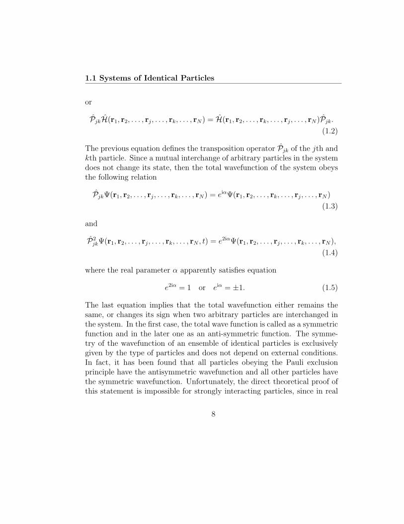
11 Systems of Identical Particles
or
PjkH(r1 r2 rj rk rN) = H(r1 r2 rk rj rN)Pjk
(12)
The previous equation defines the transposition operator Pjk of the jth andkth particle Since a mutual interchange of arbitrary particles in the systemdoes not change its state then the total wavefunction of the system obeysthe following relation
PjkΨ(r1 r2 rj rk rN) = eiαΨ(r1 r2 rk rj rN)
(13)
and
P2jkΨ(r1 r2 rj rk rN t) = e2iαΨ(r1 r2 rj rk rN)
(14)
where the real parameter α apparently satisfies equation
e2iα = 1 or eiα = plusmn1 (15)
The last equation implies that the total wavefunction either remains thesame or changes its sign when two arbitrary particles are interchanged inthe system In the first case the total wave function is called as a symmetricfunction and in the later one as an anti-symmetric function The symme-try of the wavefunction of an ensemble of identical particles is exclusivelygiven by the type of particles and does not depend on external conditionsIn fact it has been found that all particles obeying the Pauli exclusionprinciple have the antisymmetric wavefunction and all other particles havethe symmetric wavefunction Unfortunately the direct theoretical proof ofthis statement is impossible for strongly interacting particles since in real
8
11 Systems of Identical Particles
many-body systems is not possible to calculate exactly the total wavefunc-tion On the other hand the situation becomes tractable for the case ofnon-interacting or weakly interacting particle Therefore we at first will in-vestigate the system of spinless non-interacting identical particles and thenwe clarify the role of the interaction and spin
In the case of noninteracting particles the total Hamiltonian of the sys-tem can be expressed as a sum of single-particle Hamiltonians ie
H =Nsumj
Hj (16)
where N denotes the number if particles It is also well known that thetotal wavefunction of non-interacting particles can be written as a productof the single-particle wavefunctions namely
Ψ(r1 r2 rj rk rN) =Nprodj=1
ϕnj(rj) (17)
where nj represents the set of all quantum numbers characterizing the rele-vant quantum state of the jth particle The single-particle functions ϕnj
(rj)are of course the solutions of the stationary Schrodinger equation
Hjϕnj(rj) = εnj
ϕnj(rj) (18)
Here εnjdenote the eigenvalues of the single-particle Hamiltonian Hj so
that the eigenvalue of the total Hamiltonian is given by En1n2nN=
sumj εnj
The symmetric wavefunction describing whole system can be written in theform
Ψ(r1 r2 rj rk rN) = AsumP
ϕn1(r1)ϕn2(r2) ϕnN(rN) (19)
9
12 Heitler-London Theory of Direct Exchange
where A denotes the normalization constant and summation is performedover all possible permutation of the particles Similarly for the antisymmet-ric case we obtain the form
Ψ(r1 r2 rj rk rN) =1radicN
∣∣∣∣∣∣∣∣∣ϕn1(r1) ϕn1(r2) ϕn1(rN)ϕn2(r1) ϕn2(r2) ϕn2(rN)
ϕnN(r1) ϕnN
(r2) ϕnN(rN)
∣∣∣∣∣∣∣∣∣(110)
which is usually called as the Slater determinant It is clear that inter-changing of two particles in the system corresponds to the interchange ofrelevant rows in the determinant (110) which naturally leads to the signchange of the wavefunction Moreover if two or more particles occupy thesame state then two or more rows in the determinant (110) are equal andconsequently the resulting wavefunction is equal to zero in agreement withthe Pauli exclusion principle
Until now we have considered a simplified system of non-interacting par-ticles and we have completely neglected spin degrees of freedom Howeverthe situation in realistic experimental systems is much more complicatedsince each particle has a spin and moreover the interactions between parti-cles often also substantially influence the behavior of the system Howeverif we assume the case of weak interactions and if we neglect the spin-orbitinteractions then the main findings discussed above remain valid and more-over the existence of the exchange interaction can be clearly demonstratedInstead of developing an abstract and general theory for such a case itis much more useful to study a typical realistic example of the hydrogenmolecule which illustrates principal physical mechanisms leading to theappearance of magnetism
10
12 Heitler-London Theory of Direct Exchange
12 Heitler-London Theory of Direct Exchange
In the previous part we have found that the total wavefunction of themany-electron system must be anti-symmetric In this subsection we willdemonstrate that the use of anti-symmetric wave functions leads to thepurely quantum contribution to the energy of the system which is calledthe exchange energy In fact this energy initiates a certain ordering ofthe spins ie it may lead to the magnetic order in the system A similareffect we also obtain using the single-product wavefunctions if we explicitlyinclude the exchange-interaction term into Hamiltonian This effect wasindependently found by Heisenberg and Dirac in 1926 and it represent themodern quantum-mechanical basis for understanding magnetic propertiesin many real systems
a b
2
1
r
rrab
r r
ra
a
1
2 2b
21
1b
Figure 11 Schematic geometry of the H2 molecule The larger circles denotethe protons and the smaller ones represent two electrons The relevant distancesbetween different pairs of particles are denoted as rij where i j = a b 1 2
We start our analysis with one of the simplest possible system namely
11
12 Heitler-London Theory of Direct Exchange
H2 molecule In the hydrogen molecule two electrons interact with eachother and with the nuclei of the atoms The situation is schematicallydepicted in Fig11 and considering this geometry we can write the Hamil-tonian of the H2 molecule in the form
H = H1 + H2 + W + HLS (111)
where
H1 = minus ~2
2m∆1 minus
e20ra1
(112)
H2 = minus ~2
2m∆2 minus
e20rb2
(113)
W =e20rab
+e20r12
minus e20rb1
minus e20ra2
(114)
and we have used the abbreviation e0 = e(4πε0) The terms H1 and H2 in(111) describe the situation when the two hydrogen atoms are isolated Theoperator W describes the interaction between two cores electrons as wellas between electrons and relevant nuclei Finally the last term representsthe spin-orbit interaction which is assumed to be small so that we canseparate the orbital and spin degrees of freedom To solve the problem of thehydrogen molecule we apply the first-order perturbation theory neglectingthe spin-orbit coupling and taking the term W as a small perturbationAs it is usual in the perturbation theory we at first solve the unperturbedproblem ie the system of two non-interacting hydrogen atoms Thus wehave to solve the Schrodinger equation
(H1 + H2)Ψ = U0Ψ (115)
12
12 Heitler-London Theory of Direct Exchange
As we already have noted above we will assume that the total wave functioncan be written as a product of the orbital and spin functions ie Ψ =φ(r1 r2)χ(s
z1 s
z2) Another very important point to be emphasized here
is that our simplified Hamiltonian does not explicitly depend on the spinvariables Consequently we can at first evaluate only the problem withorbital functions and at the end of the calculation we can multiply theresult by an appropriate spin function to ensure the anti-symmetry of thetotal wavefunction In order to express this situation mathematically weintroduce the following notations
bull ϕα(ri)where α = a b i = 1 2 represents the orbital wave func-tion of the isolated hydrogen atom when the ith electron is localizedclosely to the αth nucleus
bull ξγ(i)where γ =uarr darr i = 1 2 is the spin function describing thespin up or spin down of the ith electron
Now let us proceed with the discussion of the orbital functions of the systemdescribed by Eq(115) Since the orbital functions ϕα(ri) are eigenfunctionsof the relevant one-atom Schrodinger equation with the same eigenvalueE0 = minus1355 eV it is clear that the ground state of the two noninteractinghydrogen atoms has the energy U0 = 2E0 and it is doubly degeneratedThis is so-called exchange degeneracy and two wavefunctions correspondingto this U0 can be expressed as φ1(r1 r2) = ϕa(r1)ϕb(r2) and φ2(r1 r2) =ϕa(r2)ϕb(r1)
If we include into Hamiltonian also the interaction term W then the sit-uation becomes much more complex and the eigenfunctions and eigenvaluescannot be found exactly In the spirit of the perturbation theory we willassume that the wavefunction of the interacting system can be expressed inthe form
φ(r1 r2) = c1φ1(r1 r2) + c2φ2(r1 r2)
= c1ϕa(r1)ϕb(r2) + c2ϕa(r2)ϕb(r1) (116)
13
12 Heitler-London Theory of Direct Exchange
where c1 and c2 are the constant that will be determined later The systemis now described by the following Schrodinger equation(H1 + H2 + W
)[c1φ1(r1 r2) + c2φ2(r1 r2
]= E
[c1φ1(r1 r2) + c2φ2(r1 r2)
](117)
Multiplying the previous equation by φlowast1(r1 r2) and integrating over the
space one obtains
2c1E0 + 2c2E0
intintφlowast1(r1 r2)φ2(r1 r2)dV1dV2
+ 2c1
intintφlowast1(r1 r2)Wφ1(r1 r2)dV1dV2 + c2
intintφlowast1(r1 r2)Wφ2(r1 r2)dV1dV2
= c1E + c2E
intintφlowast1(r1 r2)φ2(r1 r2)dV1dV2 (118)
Similarly by multiplying Eq(117) by φlowast2(r1 r2) and integrating over the
space one finds
c1E0
intintφlowast2(r1 r2)φ1(r1 r2)dV1dV2 + c1
intintφlowast2(r1 r2)Wφ1(r1 r2)dV1dV2
+ 2c2E0 + c2
intintφlowast2(r1 r2)Wφ2(r1 r2)dV1dV2
= c1E
intintφlowast2(r1 r2)φ1(r1 r2)dV1dV2 + c2E (119)
Here one should notice that in deriving Eqs(118) and (119) we have usednormalization conditions for φ1 and φ2
In order to express two previous equations in an abbreviated form oneintroduces the following quantities
1 The overlap integral
S0 =
intϕlowasta(ri)ϕb(ri)dVi i = 1 2 (120)
14
12 Heitler-London Theory of Direct Exchange
2 The Coulomb integral
K =
intintφlowast1(r1 r2)Wφ1(r1 r2)dV1dV2 =
intintφlowast2(r1 r2)Wφ2(r1 r2)dV1dV2
(121)
3 The exchange integral
A =
intintφlowast1(r1 r2)Wφ2(r1 r2)dV1dV2 =
intintφlowast2(r1 r2)Wφ1(r1 r2)dV1dV2
(122)
Applying this notation we rewrite Eqs(118) and (119) in the form
c1(2E0 +K minus E) + c2(2E0S20 + Aminus ES2
0) = 0
c1(2E0S20 + Aminus ES2
0) + c2(2E0 +K minus E) = 0 (123)
This is a homogeneous set of equations which determines unknown coeffi-cients c1 and c2 Of course we search for non-trivial solutions that can benaturally determined from the equation∣∣∣∣ 2E0 +K minus E 2E0S
20 + Aminus ES2
0
2E0S20 + Aminus ES2
0 2E0 +K minus E
∣∣∣∣ = 0 (124)
From this equation we easily find two possible solutions for the energy Eand the coefficients ci namely
Ea = 2E0 +K minus A
1minus S20
c1 = minusc2 (125)
and
Es = 2E0 +K + A
1 + S20
c1 = c2 (126)
15
12 Heitler-London Theory of Direct Exchange
Finally from the normalization condition of the total wavefunction oneobtains
1 =
int intφlowast(r1 r2)φ(r1 r2)dV1dV2
= 2|c1|2(1∓ S2) (127)
or
c1 =1radic
2(1∓ S20) (128)
where the minus and + sign corresponds to Ea and Es respectively Using(128) we can express the orbital part of the total wavefunctions as
φ(r1 r2) =1radic
2(1minus S20)
[ϕa(r1)ϕb(r2)minus ϕa(r2)ϕb(r1)
](129)
which is clearly the anti-symmetric expression and it corresponds to EaSimilarly the symmetric orbital function which corresponds to Es is givenby
φ(r1 r2) =1radic
2(1 + S20)
[ϕa(r1)ϕb(r2) + ϕa(r2)ϕb(r1)
] (130)
Finally we also can account for the spins of the electrons and to con-struct the following anti-symmetric wavefunctions
Ψ =1radic
2(1minus S20)
∣∣∣∣ ϕa(r1) ϕa(r2)ϕb(r1) ϕb(r2)
∣∣∣∣ ξuarr(1)ξuarr(2) S = 1 Sz = 1 (131)
Ψ =1radic
2(1minus S20)
∣∣∣∣ ϕa(r1) ϕa(r2)ϕb(r1) ϕb(r2)
∣∣∣∣ ξdarr(1)ξdarr(2) S = 1 Sz = 0 (132)
16
12 Heitler-London Theory of Direct Exchange
Ψ =1radic
2(1minus S20)
∣∣∣∣ ϕa(r1) ϕa(r2)ϕb(r1) ϕb(r2)
∣∣∣∣ 1radic2[ξuarr(1)ξdarr(2) + ξdarr(1)ξuarr(2)]
S = 1 Sz = minus1 (133)
and
Ψ =1radic
2(1 + S20)
[ϕa(r1)ϕb(r2) + ϕb(r1)ϕa(r2)
] 1radic2
∣∣∣∣ ξuarr(1) ξuarr(2)ξdarr(1) ξuarr(2)
∣∣∣∣S = 0 Sz = 0 (134)
Here the wavefunctions (131)-(133) form a triplet (threefold degeneratestate) with the energy Ea the total spin S = 1 and the total zth componentSz = plusmn1 0 Similarly the wavefunction (134) describes a singlet state withenergy Es the total spin S = 0 and Sz = 0 Of course both the triplet andsinglet states can be the ground state of the system depending on the signof the exchange integral In order to prove this statement we calculate theenergy difference between Ea and Es ie
∆E = Ea minus Es =2(KS2
0 minus A)
1minus S40
asymp minus2A (135)
where we have neglected the overlap integral which very small in comparisonwith other terms in the expression It is clear from the previous equationthat for A gt 0 the ground state of the system will be represented by thetriplet state with parallel alignment of spins and for A lt 0 the singlet statewith anti-parallel orientation of the spins Of course the parallel (anti-parallel) spin orientation implies also parallel (anti-parallel) alignment of themagnetic moments which is crucial for the observation of the ferromagneticor antiferromagnetic ordering in the real systems
The situation in the hydrogen molecule of course differs from the realsituation in ionic crystal in many respects For example the electrons in
17
12 Heitler-London Theory of Direct Exchange
the hydrogen molecule occupy 1s orbitals while in the ionic crystals theunpaired localized electrons usually occupy d or f orbitals In fact thecalculation of the exchange integral using 3d orbital functions leads to thepositive value of the A Therefore the direct exchange interactions leadsto the ferromagnetic ordering in such systems Later it was discovered byAnderson that the antiferromagnetic ordering is caused by so-called indi-rect exchange interaction via a non-magnetic bridging atom The situationin real materials is usually much more complicated and other mechanismsuch as the Dzyaloshinkii-Moriya or Ruderman-Kittel-Kasuya-Yosida inter-actions can play an important role
Although the calculation performed for the hydrogen molecule does notreflect the complex situation of the real magnetic systems it is extremelyimportant from the methodological point of view In fact it is clear from ourcalculation that the parallel or anti-parallel alignment of the magnetic mo-ments appears due to new contribution to the energy of the system whichoriginates from the indistinguishability of quantum particles The othermechanisms leading to the macroscopic magnetism have also quantum na-ture and cannot be included into the classical theory
Thus we can conclude that the physical origin of magnetism can becorrectly understood and described only within the quantum theory
18
Chapter 2
Bogolyubov Inequality and ItsApplications
21 General Remarks on Bogolyubov Inequal-
ity
The Bogolyubov inequality for the Gibbs free energy G of an interactingmany-body system described by the Hamiltonian H is usually written inthe form
G le G0 + ⟨H minus H0⟩0 = ϕ(λx λy λz ) (21)
In this equation the so-called trial Hamiltonian H0 = H0(λx λy λz )depends on some variational parameters λi that are naturally determinedin the process of calculation and the symbol ⟨ ⟩0 stands for the usualensemble average calculated with the trial Hamiltonian Finally G0 denotesthe Gibbs free energy of the trial system defined by
G0 = G0(λx λy λz ) = minus 1
βlnZ0 (22)
19
22 Mean-Field Theory of Anisotropic Heisenberg Model
where β = 1kBT and the the partition function Z0 is given by
Z0 = Tr eminusβH0 (23)
In general there is a remarkable freedom in defining the trial Hamilto-nian In fact the only limitations to be taken into account follow from thetwo obvious requirements
1 The trial Hamiltonian should naturally represent a simplified physicalmodel of the real system
2 The expression of G0 must be calculated exactly in order to obtain aclosed-form formula for the rhs of Eqs(21)
22 Mean-Field Theory of the Spin-12
Anisotropic Heisenberg Model
221 General Formulation
The accurate theoretical analysis of the Heisenberg model is extremely harddue to interaction terms in the Hamiltonian including non-commutative spinoperators Probably the simplest analytic theory applicable to the modelis the standard mean-field approach Although the mean-field theory canmathematically be formulated in many different ways we will develop in thistext an approach based on the Bogolyubov inequality for the free energy ofthe system The main advantage of this formulation is its completeness (wecan derive analytic formulas for all thermodynamic quantities of interest)and a possibility of further generalizations for example an extension to theOguchi approximation
20
22 Mean-Field Theory of Anisotropic Heisenberg Model
In this part we will study the spin-12 anisotropic Heisenberg model ona crystal lattice described by the Hamiltonian
H = minussumij
(JxSxi S
xj + JyS
yi S
yj + JzS
zi S
zj )minus gmicroB
sumi
(HxSxi +HyS
yi +HzS
zi )
(24)where g is the Lande factor microB is the Bohr magneton Jα and Hα α =x y z denote the spatial components of the exchange interaction and exter-nal magnetic field respectively One should note here that Jα is assumedto be positive for the ferromagnetic systems and negative for the antifer-romagnetic ones Moreover it is well-known that the absolute value ofexchange integrals very rapidly decreases with the distance thus we canrestrict the summation in the first term of (24) to the nearest-neighboringpairs of atoms on the lattice Finally the spatial components of the spin-12operators are given by
Sxk =
1
2
(0 11 0
)k
Syk =
1
2
(0 minusii 0
)k
Szk =
1
2
(1 00 minus1
)k
(25)
To proceed further we choose the trial Hamiltonian in the form
H0 = minusNsumk
(λxS
xk + λyS
yk + λzS
zk
) (26)
where N denotes the total number of the lattice sites and λi are variationalparameters to be determined be minimizing of the rhs of the Bogolyubovinequality After substituting (25) into (26) we can apparently rewriteprevious equation as follows
H0 =Nsumk=1
H0k (27)
21
22 Mean-Field Theory of Anisotropic Heisenberg Model
where the site Hamiltonian H0k is given by
H0k = minus1
2
(λz λx minus iλy
λx + iλy minusλz
)k
(28)
In order to evaluate the terms entering the Bogolyubov inequality we atfirst have to calculate the partition function Z0 Taking into account thecommutation relation [H0k H0ℓ] = 0 for k = ℓ we obtain the followingexpression
Z0 = Tr exp(minusβ
Nsumk=1
H0k
)=
Nprodk=1
Trk exp(minusβH0k
) (29)
where Trk denotes the trace of the relevant operator related to kth latticesite Now after setting Eq(28) into (29) one obtains
Z0 =Nprodk=1
Trk exp
(β2λz
β2(λx minus iλy)
β2(λx + iλy) minusβ
2λz
)k
=
[Trk exp
(β2λz
β2(λx minus iλy)
β2(λx + iλy) minusβ
2λz
)k
]N
(210)
The crucial point for further calculation is the evaluation of exponentialfunction in previous equation Let us note that in performing this task wewill not follow the usual approach based on the diagonalization of modifiedmatrix (28) entering the argument of exponential Instead we will performall calculations in the real space by applying the following matrix form ofthe Cauchy integral formula
eminusβH0k =1
2πi
∮C
ezdz
zI minus (minusβH0k) (211)
22
22 Mean-Field Theory of Anisotropic Heisenberg Model
After a straightforward calculation we obtain
eminusβH0k =
(h11 h12
h21 h22
)(212)
with
h11 = cosh
(β
2Λ
)+
λz
Λsinh
(β
2Λ
)(213)
h12 =λx minus iλy
Λsinh
(β
2Λ
)(214)
h21 =λx + iλy
Λsinh
(β
2Λ
)(215)
h22 = cosh
(β
2Λ
)minus λz
Λsinh
(β
2Λ
) (216)
where we have introduced the parameter
Λ =radicλ2x + λ2
y + λ2z (217)
Using previous equations we easily obtain the following expressions for Z0
and G0
Z0 =
[2 cosh
(β
2Λ
)]N(218)
G0 = minusN
βln
[2 cosh
(β2Λ
)] (219)
23
22 Mean-Field Theory of Anisotropic Heisenberg Model
To obtain the complete expression for ϕ(λx λy λz ) we have to eval-
uate the terms ⟨H⟩0 and ⟨H0⟩0 that can be expressed as
⟨H⟩0 = minusNq
2
(Jx⟨Sx
i Sxj ⟩0 + Jy⟨Sy
i Syj ⟩0 + Jz⟨Sz
i Szj ⟩0
)minus N
(hx⟨Sx
j ⟩0 + hy⟨Syj ⟩0 + hz⟨Sz
j ⟩0) (220)
where q denotes the coordination number of the lattice and hα = gmicroBHα(α = x y z) Similarly we have
⟨H0⟩0 = minusN(λx⟨Sx
j ⟩0 + λy⟨Syj ⟩0 + λz⟨Sz
j ⟩0) (221)
The ensemble averages of ⟨Sαj ⟩0 entering two previous equations can be
expressed in the form
⟨Sαj ⟩0 =
1
Z0
TrSαj e
minusβH0
=TrjS
αj exp
(minusβH0j
)prodNminus1k =j Trk exp
(minusβH0k
)Trj exp
(minusβH0j
)prodNminus1k =j Trk exp
(minusβH0k
) (222)
which can be simplified as follows
⟨Sαj ⟩0 =
TrjSαj exp
(minusβH0j
)Trj exp
(minusβH0j
) (223)
Similarly one easily finds that
⟨Sαi S
αj ⟩0 =
TriSαi exp
(minusβH0i
)Tri exp
(minusβH0i
) TrjSαj exp
(minusβH0j
)Trj exp
(minusβH0j
) =(⟨Sα
j ⟩0)2
(224)
24
22 Mean-Field Theory of Anisotropic Heisenberg Model
In order to complete our calculation we substitute Eqs (212)-(216) intoEq (223) and then we evaluate the trace of relevant matrices In this waywe obtain the following equation
⟨Sαj ⟩0 =
λα
2Λtanh
(β
2Λ
) (225)
and
⟨Sαi S
αj ⟩0 =
(λα
2Λ
)2
tanh2
(β
2Λ
) (226)
After introducing notation ⟨Sαj ⟩0 = mα α = x y z we can rewrite the rhs
of the Bogolyubov inequality in the form
ϕ(λx λy λz) = minusN
βln(2 cosh
β
2Λ)minus Nq
2
(Jxm
2x + Jym
2y + Jzm
2z
)+ N
[(λx minus hx)mx + (λy minus hy)my + (λz minus hz)mz
] (227)
Since the quantity ϕ represents an upper bound for the exact Gibbs freeenergy of the system then the best possible approximation (with the trialHamiltonian H0) corresponds for those values of λx λy λz that minimizeϕ(λx λy λz) Relevant values of λx λy λz are obviously determined fromthe equations
partϕ
partλx
= 0partϕ
partλy
= 0partϕ
partλz
= 0 (228)
The above conditions lead to three independent equations that can berewritten in the following simple matrix form
partmx
partλx
partmy
partλx
partmz
partλxpartmx
partλy
partmy
partλy
partmz
partλy
partmx
partλz
partmy
partλz
partmz
partλz
λx minus qJxmx minus hx
λy minus qJymy minus hy
λz minus qJzmz minus hz
= 0 (229)
25
22 Mean-Field Theory of Anisotropic Heisenberg Model
Since the first matrix in (229) is in general non-zero then the only possiblesolution of this equation is given by
λx = qJxmx + hx λy = qJymy + hy λz = qJzmz + hz (230)
and the cooresponding equilibrium Gibbs free energy can be after a smallmanipulation expressed in the form
G = minusN
βln2 cosh
(βhef
2
)+
Nq
2
(Jxm
2x + Jym
2y + Jzm
2z
) (231)
where we have denoted
hef =radic
(qJxmx + hx)2 + (qJymy + hy)2 + (qJzmz + hz)2 (232)
Having obtained the last equation we are able to identify the physicalmeaning of the parameters mxmymx and consequently also the meaningof variational parameters λx λy λz
For this purpose we at first recall that the spatial component of thetotal magnetization Mα is defined as
Mα = minus(
partGpartHα
)β
= minusgmicroB
(partGparthα
)β
(233)
After a straightforward calculation we obtain the following very simple ex-pressions
Mx
NgmicroB
= mx = ⟨Sxj ⟩0
My
NgmicroB
= my = ⟨Syj ⟩0
Mz
NgmicroB
= mz = ⟨Szj ⟩0
(234)
which clearly indicate that mα represents the spatial components of themagnetization Consequently the parameters λα have the meaning of ofthe molecular-field components acting on one atom in the lattice Thusour formulation is nothing but the standard mean-field theory The mainadvantage of our approach is that this formulation provides a close-form an-alytical expression for the Gibbs free energy which is of principal importancefor finding stability conditions of various physical quantities
26
22 Mean-Field Theory of Anisotropic Heisenberg Model
222 Thermodynamic Properties of the HeisenbergModel
Now let us proceed with the calculation of several interesting physical quan-tities for the system under investigation Using Eqs (222) (230) and(234) one simply obtains for the components of reduced magnetization aset of three coupled equations namely
mx =qJxmx + hx
2hef
tanh
(β
2hef
) (235)
my =qJymy + hy
2hef
tanh
(β
2hef
) (236)
mz =qJzmz + hz
2hef
tanh
(β
2hef
) (237)
where we have denotedIn order to investigate the long-range ordering the systems we set hx =
hy = hz = 0 and obtain
mx =Jxmx
2h0
tanh
(βq
2h0
) (238)
my =Jymy
2h0
tanh
(βq
2h0
) (239)
mz =Jzmz
2h0
tanh
(βq
2h0
) (240)
27
22 Mean-Field Theory of Anisotropic Heisenberg Model
with
h0 =radic(Jxmx)2 + (Jymy)2 + (Jzmz)2 (241)
These three nonlinear equations have always the trivial solution mx =my = mz = 0 corresponding to the disordered paramagnetic phase (DP)Moreover depending on the temperature and the values of exchange pa-rameters there also exist non-trivial solutions corresponding to ordered fer-romagnetic phase (OP) The stability of the relevant solutions is then de-termined by the minimum of the Gibbs free energy given by Eq(231) Nowwe briefly analyze possible trivial and non-trivial solutions of (238)-(240)for some particular cases of the exchange interactions
1 Ising model Jx = Jy = 0 Jz = J = 0
mx = my = 0 and mz =1
2tanh
(qβJ2
mz
)for T lt Tc
mx = my = mz = 0 for T gt Tc (242)
2 Isotropic XY model Jx = Jy = J = 0 Jz = 0
mz = 0my = mx and mx =1
2radic2tanh
(radic2qβJ
2mx
)for T lt Tc
mx = my = mz = 0 for T gt Tc (243)
3 Isotropic Heisenberg model Jx = Jy = Jz = 0
my = mx = mz and mz =1
2radic3tanh
(radic3qβJx2
mx
)for T lt Tc
mx = my = mz = 0 for T gt Tc (244)
28
22 Mean-Field Theory of Anisotropic Heisenberg Model
Here one should note that non-trivial results for isotropic XY and Heisen-berg model model represents valid solution for the models when the axis ofquantization is given by the equation y = x = t t isin R for the XY modeland y = x = z = t t isin R for the Heisenberg model On the other handif choose as a quantization axis for example the x axis then we obtain forboth models identical result as that for the Ising one Thus one can concludethat mean-field theory is not able to describe correctly quantum featuresof localized spin models In order to illustrate the numerical accuracy ofthe method we have compared in Fig 23 the temperature variation of themean-field magnetization with exact result on the square lattice with q = 4
00 05 10 15000
025
050q = 4
m
kBT J
Exact
MFT
Figure 21 Comparisom of the temperature dependence of magnetization forthe Ising model on a square lattice
The critical (or Curie) temperature is defined as a temperature at whichthe long-range order (or magnetization) vanishes In order to determine the
29
22 Mean-Field Theory of Anisotropic Heisenberg Model
Curie temperature we take into account that tanh(x) asymp x for x ltlt 1 andobtain an universal solution
Tc =qJα
4kB α = x y z (245)
which valid for all three cases mentioned above Of course the critical tem-perature should be different depending on the model considered Thus thepresent method is not able to distinguish specific features of the models aslong as concerns the critical behavior Moreover it is also clear that thetopology of the lattice is taken into account only through its coordinationnumber that is also weak point of the present method It is well knownthat this approach significantly fails for the low-dimensional systems nev-ertheless it gives rather good qualitative picture for the three-dimensionalsystems and therefore it is frequently used to obtain analytical results par-ticularly for complex systems
Finally one should note that calculations of other thermodynamic quan-tities is easy and straightforward since we have analytical solution for theGibbs free energy of the system from which other quantities are easily ob-tained
This calculation including numerical analysis and discussion is left forthe readers as an appropriate exercise
Let us conclude this part by noticing that the present approach can beextended to case of the the so-called Oguchi approximation which alreadyaccount much better for the quantum effects as well as for the spin-spincorrelations Possible extensions are rather involved and require lengthycalculations that are beyond the scope of the present book
30
Chapter 3
Spin-Wave Theory
31 Bloch Spin-Wave Theory of Ferromag-
nets
In this part we will discuss the concept of spin waves which enables to studythe some physical properties of magnetic systems at low temperatures Thistheory was originally introduced by F Bloch [1] and its main assumptionis that the ground state of the system is ordered and the excited states aredescribed as a collection of spin waves At low temperatures it is reasonableto expect the small amplitudes of the spin waves thus the interaction amongspin waves can be neglected We will consider in this part an isotropicHeisenberg model defined by the Hamiltonian
H = minusJsumij
SiSj minus gmicroBHsumi
Szi (31)
Here Si represents a vector spin-operator at the ith site of the lattice Thisoperator is naturally defined as Si = (Sx
i Syi S
zi ) where Sα
i (α = x y z)represent spatial components of the standard spin operators g is the Lande
31
31 Bloch Spin-Wave Theory of Ferromagnets
factor microB is the Bohr magneton and H denotes the external magnetic fieldwhich is applied along z axis J is the exchange integral which is assumedto be positive since we are going to investigate the ferromagnetic systems
Adopting the basic concept of lattice vibrations we can write the fol-lowing equation of motion of the spin Sℓ on the j th lattice point
dSℓ
dt=
i
~[H Sℓ] (32)
In what follows we will use the following commutation relations for spinoperators
[Sai S
bj ] = iεabcδijS
cj a b c = x y or z (33)
where εabc represents Levi-Civita tensor and δij is the Kronecker symbolNow substituting the Hamiltonian (31) into (32) and employing relations(33) one obtains
dSℓ
dt= minus1
~(Hℓ times Sℓ) (34)
where the local magnetic field Hℓ acting on the j th spin is given by
Hℓ =sumj
JjℓSj + gmicroBHe3 (35)
with e3 = (0 0 1) Using two previous equations one easily obtains thefollowing equations of motion of the x y and z components of the spinoperator
~dSx
ℓ
dt= minus
sumj
Jjℓ(Syj S
zℓ minus Sz
j Syℓ ) + gmicroBHSy
ℓ (36)
~dSy
ℓ
dt= minus
sumj
Jjℓ(Szj S
xℓ minus Sx
j Szℓ )minus gmicroBHSx
ℓ (37)
32
31 Bloch Spin-Wave Theory of Ferromagnets
~dSz
ℓ
dt= minus
sumj
Jjℓ(Sxj S
yℓ minus Sy
j Sxℓ ) (38)
If we restrict ourselves to the case of low-energy excitation then the compo-nents Sx
ℓ Syℓ can be regarded as small quantities of first order Consequently
the right-hand side of (38) is a small quantity of the second order whichcan be neglected and it follows from Eq (38) that the zth component be-comes a constant Moreover it is reasonable to put explicitly Sz
ℓ = S sincethe external magnetic field is assumed to be applied parallel to the zth axisUnder these assumptions Eqs (36) and (37) can be rewritten in the form
~dSx
ℓ
dt= minusS
sumj
Jjℓ(Syj minus Sy
ℓ ) + gmicroBHSyℓ (39)
~dSy
ℓ
dt= minusS
sumj
Jjℓ(Sxℓ minus Sx
j )minus gmicroBHSxℓ (310)
or alternatively
~dS+
ℓ
dt= minusiS
sumj
Jjℓ(S+ℓ minus S+
j )minus gmicroBHS+ℓ (311)
~dSminus
ℓ
dt= minusiS
sumj
Jjℓ(Sminusℓ minus Sminus
j )minus gmicroBHSminusℓ (312)
where we have introduced the spin-raising and spin-lowering operators
S+ℓ = Sx
ℓ + iSyℓ Sminus
ℓ = Sxℓ minus iSy
ℓ (313)
that obey the following commutation rules
[Szk S
+ℓ ] = S+
k δkℓ [Szk S
minusℓ ] = minusSminus
k δkℓ [S+k S
+ℓ ] = 2Sz
kδkℓ (314)
33
31 Bloch Spin-Wave Theory of Ferromagnets
The above relations are directly obtained with the help of well-known com-mutation relations of the spin operators (33)
To proceed further we now express the spin-raising and spin-loweringoperators with the help of the Fourier transform ie
S+q =
1radicN
sumj
eiqmiddotRj S+j Sminus
q =1radicN
sumj
eminusiqmiddotRj Sminusj (315)
S+j =
1radicN
sumq
eminusiqmiddotRj Sq Sminusj =
1radicN
sumq
eiqmiddotRj Sq (316)
Substituting Eq(316) into Eq(312) and applying the following relationsumℓ
eminusi(q1minusq2)middotRℓ = Nδq1q2 (317)
one gets equation
minusi~dSminus
q
dt=
[Ssumℓ
Jjℓ(1minus eminusiqmiddot(RjminusRℓ)) + gmicroBH]Sminusq (318)
If we now introduce a real quantity
J(q) =sumj
J(Rj)eminusiqmiddotRj (319)
then we rewrite (318) as
minusi~dSminus
q
dt=
S[J(0)minus J(q)
]+ gmicroBH
Sminusq (320)
It is straightforward to obtain the solution of this equation in the form
Sq = δSqei(ωqt+α) (321)
34
31 Bloch Spin-Wave Theory of Ferromagnets
where the eigenfrequencies of the spin waves are given by
~ωq = S[J(0)minus J(q)
]+ gmicroBH (322)
One should notice here that in the limit of small q we obtain ~ωq asymp q2Now using Eq(321) we can express the spin operators in the real space
as follows
Sminusj =
1radicNδSqe
i(qmiddotRj+ωqt+α) (323)
Sxj =
1radicNδSq cos
[i(q middotRj + ωqt+ α)
](324)
and
Syj = minus 1radic
NδSq sin
[i(q middotRj + ωqt+ α)
] (325)
Finally it is straightforward to prove that the energy difference betweenan excited state and ground state is given by
Eq minus E0 = ~ωq (326)
where ~ωq represents the excitation energy of the spin wave with the wavevec-tor q The proof of the last statement is left as an appropriate exercise forreaders
35
32 Holstein-Primakoff theory of ferromagnets
32 Holstein-Primakoff theory of ferromag-
nets
The Blochrsquos spin-wave theory discussed in previous chapter represents a verysimple approach in which we completely neglect the interaction among spinwaves This deficiency can be eliminated using an alternative formulationbased on magnon variables (or creation-annihilation operators) developedby Holstein and Primakoff [2] In this part we apply The Holstein-Primakofftheory to case of an anisotropic quantum Heisenberg model described bythe Hamiltonian
H = minusJsumij
(Sxi S
xj + Sy
i Syj + Sz
i Szj )minus gmicroBH
sumi
Szi (327)
The meaning of all symbols in previous Eq (327) is the same as in previoustext
In order to apply a spin-wave picture to analyze magnetic properties ofthe model under investigation one has to perform three subsequent math-ematical transformation At first we express the components of the spinoperators trough spin-lowering and spin raising operators then we intro-duce so-called creation and annihilation operators and finally we performa Fourier transform of the relevant all creation and annihilation operatorsentering the Hamiltonian The eigenvalues of the final Hamiltonian then en-able to determine relevant physical quantities applying standard relationsof statistical mechanics For further manipulations it is more convenient torewrite (327) as follows
H = minusJsumℓδ
(Sxℓ S
xℓ+δ + Sy
ℓ Syℓ+δ + Sz
ℓ Szℓ+δ)minus gmicroBH
sumℓ
Szℓ (328)
where ℓ labels the lattice sites and δ denotes nearest neighbors of the relevantsite and we assume that J gt 0 The integrals of motion for Hamiltonian
36
32 Holstein-Primakoff theory of ferromagnets
(328) are the total z th component Sz =sum
k Szk and the total spin of the
systemThe ground state of the system is ordered and for H gt 0 the magnetic
moment is paralell to the z axis If we consider the lattice consisting of Natoms with spin S then the ground-state vector in the spin basis reads |0⟩= |NSNS⟩ Of course we work in a real space basis in which the spinoperators Sz
ℓ are diagonal We recall that the eigenvalues MS = minusS minusS +1 S and eigenvectors |MS⟩ℓ of the operator Sz
ℓ satisfy the followingequation
Szℓ |MS⟩ℓ = MS|MS⟩ℓ (329)
Now applying operators (313) to the eigenvectors |MS⟩ℓ one obtains
S+ℓ |MS⟩ℓ =
radic(S minusMS)(S minusMS minus 1)|MS + 1⟩ℓ (330)
and
Sminusℓ |MS⟩ℓ =
radic(S +MS)(S minusMS minus 1)|MS minus 1⟩ℓ (331)
In addition to the spin-raising and spin-lowering operators we will alsouse in our analysis the operator describing a deviation of the zth spin-component from its maximum value namely
nℓ = S minus Szℓ (332)
The eigenvalues of this operator are integers nl = 0 1 2 2S (or nl =S minusMS) thus we can rewrite Eqs(330) in the form
S+ℓ |nℓ⟩ℓ =
radic2S
radic1minus (nℓ minus 1)
2S
radicnℓ|nℓ minus 1⟩ℓ (333)
Le us note that performing a similar procedure is also possible for Eq(331)and it will be used later
37
32 Holstein-Primakoff theory of ferromagnets
Now with the help of (313) we can rewrite the Hamiltonian (328) inthe form
H = minusJsumℓδ
[12(S+
ℓ Sminusℓ+δ + Sminus
ℓ S+ℓ+δ) + Sz
ℓ Szℓ+δ
]minus gmicroBH
sumℓ
Szℓ (334)
which is suitable for introducing the Holstein-Primakoff magnon represen-tation In order to define the relevant transformation we at first introducethe standard creation and annihilation operators that are defined as
adaggerℓΨnℓ=
radicnℓ + 1Ψnℓ+1 aℓΨnℓ
=radicnℓΨnℓminus1 (335)
The central idea of the Holstein-Primakoff approach is based on the intro-duction of the following transformation
S+ℓ = (2S)12
(1minus adaggerℓaℓ
2S
)12
aℓ (336)
Sminusℓ = (2S)12adaggerℓ
(1minus adaggerℓaℓ
2S
)12
(337)
Szℓ = S minus adaggerℓaℓ (338)
As already noted above the eigenvalues of adaggerℓaℓ are arbitrary integers whilethat of nℓ are limited to the range 0 le nℓ le 2S Fortunately this discrep-ancy does not play any important role in the calculation since the transitionfrom the state with nℓ le 2S to states with nℓ gt 2S never occur eg
Sminusℓ Ψ2S = (2S)12(2S + 1)12
(1minus 2S
2S
)12
Ψ2S+1 = 0 (339)
Now we transform the operators aℓ adaggerℓ from the real space to the reciprocal
space by the following Fourier tansform
aℓ =1radicN
sumq
eminusiqmiddotRℓbq (340)
38
32 Holstein-Primakoff theory of ferromagnets
adaggerℓ =1radicN
sumq
eiqmiddotRℓbdaggerq (341)
where N denotes the total number of atoms q represents a vector of thereciprocal space and Rℓ represents a vector specifying the position of ℓthatom in the lattice
The magnon-annihilation and magnon-creation operators are given by
bq =1radicN
sumℓ
eiqmiddotRℓaℓ (342)
bdaggerq =1radicN
sumℓ
eminusiqmiddotRℓadaggerℓ (343)
and they obey the usual magnon commutation relations
[bq1 bdaggerq2] = δq1q2 [bq1 bq2 ] = [bdaggerq1
bdaggerq2] = 0 (344)
It is useful to note here that the operator bdaggerq creates a magnon with thewave vector q and the operator bq annihilates it Moreover it follows fromthe transformation (340) and (341) that any change of the spin state atarbitrary lattice site is described as a superposition of an infinite number ofthe spin waves
At this stage it is clear that further exact treatment of the problem isimpossible due to the complexity of applied transformations The progressis however still possible if we restrict ourselves to the case when the numberof excited states is small in comparison with 2S Under this assumptionwe can neglect the higher order terms in expansion of the square root andrewrite Eqs (336) and (337) in the form
S+ℓ = (2S)12
(1minus adaggerℓaℓ
4S
)aℓ + (345)
39
32 Holstein-Primakoff theory of ferromagnets
Sminusℓ = (2S)12adaggerℓ
(1minus adaggerℓaℓ
4S
)+ (346)
Finally substituting (340) and (341) into previous equation one obtains
S+ℓ =
(2S
N
)12[sumq1
eminusiq1middotRℓbq1 minus1
4SN
sumq1q2q3
ei(q1minusq2minusq3)middotRℓbdaggerq1bq2bq3 +
](347)
Sminusℓ =
(2S
N
)12[sumq1
eiq1middotRℓbdaggerq1minus 1
4SN
sumq1q2q3
ei(q1+q2minusq3)middotRℓbdaggerq1bdaggerq2
bq3 +
](348)
Similarly the operator Szℓ is given by
Szℓ = S minus 1
N
sumq1q2
ei(q1minusq2)middotRℓbdaggerq1bq2 (349)
If we assume that each lattice site has z nearest neighbors then we canspecify their positions on the lattice by introducing the vector
δ = Rℓ+δ minusRℓ (350)
Substituting (347)-(350) into Eq(334) and performing a rearrange-ment of the terms one can rewrite the Hamiltonian as
H = minusJNzS2 minus gmicroBNHS + H0 + H1 (351)
where H0 is a bilinear form in the magnon variables and it is given by
H0 = minus JS
N
sumℓδ
sumq1q2
[eminusi(q1minusq2)middotRℓeiq2middotδbq1b
daggerq2
+ ei(q1minusq2)middotRℓeminusiq2middotδbdaggerq1bq2
]+
JS
N
sumℓδ
sumq1q2
[ei(q1minusq2)middotRℓbq1b
daggerq2
+ eminusi(q1minusq2)middotRℓei(q1minusq2)middotδbdaggerq1bq2
]+
gmicroBH
N
sumℓq1q2
ei(q1minusq2)middotRℓbdaggerq1bq2 (352)
40
32 Holstein-Primakoff theory of ferromagnets
The term H1 includes higher-order terms and for the sake of simplicity willbe neglected Now taking into account the relation (317) and performingthe summation over ℓ and q2 we can simplify Eq(352) as follows
H0 = minusJzSsumq
(γqbqbdaggerq + γminusqb
daggerqbq minus 2bdaggerqbq) + gmicroBH
sumq
bdaggerqbq (353)
where
γq =1
z
sumδ
eiqmiddotδ (354)
and the summation in (354) runs over all nearest neighbors For furthermanipulation it useful noticing that
sumq γq = 0 and moreover for the crys-
tals with the symmetry center we have γq = γminusk Employing the magnoncommutation rules [bdaggerqbq] = 1 one obtains
H0 =sumq
[2JzS(1minus γq) + gmicroBH
]bdaggerqbq (355)
The last equation can be rewritten in the following very simple form
H0 =sumq
~ωqnq (356)
where nq is the magnon occupation operator and
~ωq = 2JzS(1minus γq) + gmicroBH (357)
Since the quantity γq can be expressed as follows
γq =1
z
sumδ
eiqmiddotδ =1
2z
sumδ
(eiqmiddotδ + eminusiqmiddotδ) =1
2z
sumδ
cos(q middot δ) (358)
then the dispersion relation becomes
~ωq = 2JzS[1minus 1
2z
sumδ
cos(q middot δ)]+ gmicroBH (359)
41
32 Holstein-Primakoff theory of ferromagnets
321 Internal Energy and Specific heat
In this subsection we will show how one can calculate the internal energyand specific heat of Heisenberg model within the Holstein-Primakoff theoryBefore performing any calculation it is useful noticing that due to neglectinghigher order terms in Eq (345) and (346) we treat the ensemble of non-interacting magnons In further calculatiuon we also will assume H = 0and |q middot δ| ≪ 1
Under these assumptions the internal energy of the magnon gas in ther-modynamic equilibrium at temperature T can be expressed as
U =sumq
~ωq⟨nq⟩ (360)
where ⟨nq⟩ is given by the well-known Bose-Einstein relation
⟨nq⟩ =[exp
( ~ωq
kBT
)minus 1
]minus1
(361)
Substituting (361) into (360) one gets
U =sumq
~ωq
[exp
( ~ωq
kBT
)minus 1
]minus1
=1
(2π)3
intDq2
[exp
(Dq2
kBT
)minus 1
]minus1
d3q
=1
2π2
intDq4
[exp
(Dq2
kBT
)minus 1
]minus1
dq (362)
where we have introduced the lattice stiffnes as D = 2SJa2 If we denotex = Dq2kBT then we can rewrite (362) as
U =(kBT )
52
4π2D32
int xm
0
x32
exp(x)minus 1dx (363)
42
32 Holstein-Primakoff theory of ferromagnets
The last expression can be further simplified by considering the regionkBT ≪ ωmax Then the upper limit in the integral (363) can be approxi-mated by infinity and one obtains for internal energy the following analyticalexpression for internal energy of the system
U =(kBT )
52
4π2D32Γ(52
)ζ(52 1) (364)
Here Γ and ζ denote the Gamma- and Riemann zeta-functions respectively
and their numerical values of relevant arguments are known to be Γ(
52
)=
3radicπ
4and ζ
(52 1)= 1341
Thus we finally obtain
U ≃ 045(kBT )52
π2D32 (365)
Consequently for the magnetic part of specific heat at constant volume isgiven by
CV = 0113kB
(kBTD
) 32 (366)
In this work we consider strictly insulating materials thus there is no elec-tron contribution to the total specific heat Consequently taking into ac-count the phonon and magnon contribution we can express the total specificheat at low temperatures by the formula
C = aT 3 + bT 32 (367)
It is clear from this equation that the magnon contribution can experimen-tally easily determined if we plot the dependence of reduced specific heatCT 32 versus T 32 The situation is schematically illustrated in Fig 31
43
32 Holstein-Primakoff theory of ferromagnets
0 2 4 6 80
1
2
CT -32
T 32
magnoncontribution
Figure 31 The re-scaled specific heat vs T 32
322 Magnetization and Critical Temperature
The magnetic moment of the system can be calculated from the equation
MS = gmicroB
⟨(NS minus
sumq
bdaggerqbq)⟩ (368)
The deviation of the magnetization from its saturation value can be ex-pressed as
∆M = M(0)minusM(T ) = gmicroB
sumq
⟨nq⟩
=gmicroB
(2π)3
int qm
0
[exp
(Dq2
kBT
)minus 1
]minus1
d3q (369)
44
33 Holstein-Primakoff theory of antiferromagnets
At low temperatures (Dq2 ≫ kBTJ) we obtain
∆M =gmicroB
2π2
(kBTJD
)32int infin
0
x12
exp(x)minus 1dx
=gmicroB
2π2
(kBTJD
)32
Γ(52
)ζ(32 1)
= 0117gmicroB
(kBTD
)32
(370)
The finite-temperature magnetization can be then expressed as
M(T ) = M(0)[1minus
( T
Tc
) 32]
(371)
where the critical temperature Tc is given by
Tc =( M(0)
0117gmicroB
) 23 D
kB (372)
33 Holstein-Primakoff theory of antiferro-
magnets
The Holstein-Primakoff theory can be extended also to the case of antifero-magnetic Heisenberg model which can describe many real materials [7] Onthe other hand the generalization of the Holstein-Primakoff for quantumantiferromagnets is very interesting because such systems exhibit very inter-esting magnetic properties that differ from quantum ferromagnets in manyrespects Our aim in this subsection is to investigate the antiferromagneticHeisenberg model spin system consisting of two interpenetrating sublatticesa and b which is described by the Hamiltonian
H = minusJsumij
SaiSbj minus gmicroBHa
sumi
Szai + gmicroBHa
sumj
Szbj (373)
45
33 Holstein-Primakoff theory of antiferromagnets
where J lt 0 is the exchange interaction which couples the nearest neighborson lattice and the quantity Ha gt 0 represents an external magnetic fieldwhich is parallel to the z axis In what follows we will treat the problem ap-plying the Holstein-Primakoff transformation for each sublattice separatelyAt first we express the spin rising and lowering sublattice operators withthe help of creation-annihilation operators as follows
S+aj = (2S)12
(1minus
adaggerjaj
2S
)12
aj Sminusaj = (2S)12adaggerj
(1minus
adaggerjaj
2S
)12
(374)
S+bℓ = (2S)12
(1minus bdaggerℓbℓ
2S
)12
bℓ Sminusbℓ = (2S)12bdaggerℓ
(1minus bdaggerℓbℓ
2S
)12
(375)
Szaj = S minus adaggerjaj minusSz
bℓ = S minus bdaggerℓbℓ (376)
Next we introduce the sublattice spin-wave variables
cq =2radicN
sumj
eminusiqmiddotRjaj cdaggerq =2radicN
sumj
eiqmiddotRjadaggerj (377)
dq =2radicN
sumℓ
eiqmiddotRℓbℓ ddaggerq =2radicN
sumℓ
eminusiqmiddotRℓbdaggerℓ (378)
In previous equations summations run over all N atoms of the a and b sub-lattice respectively Moreover the following magnon commutation relationshold
[cq1 cdaggerq2] = [dq1 d
daggerq2] = δq1q2
[cq1 cq2 ] = [cdaggerq1 cdaggerq2
] = 0 [dq1 dq2 ] = [ddaggerq1 ddaggerq2
] = 0 (379)
46
33 Holstein-Primakoff theory of antiferromagnets
Now we expand (374)-(375) as
S+aj =
(4S
N
)12[sumq1
eminusiq1middotRjcq1 minus1
8SN
sumq1q2q3
ei(q1minusq2minusq3)middotRjcdaggerq1cq2cq3 +
](380)
Sminusaj =
(4S
N
)12[sumq1
eiq1middotRjcdaggerq1minus 1
8SN
sumq1q2q3
ei(q1+q2minusq3)middotRjcdaggerq1cdaggerq2
cq3 +
](381)
S+bℓ =
(4S
N
)12[sumq1
eminusiq1middotRℓdq1 minus1
8SN
sumq1q2q3
ei(q1minusq2minusq3)middotRℓddaggerq1dq2dq3 +
](382)
Sminusbℓ =
(4S
N
)12[sumq1
eiq1middotRℓddaggerq1minus 1
8SN
sumq1q2q3
ei(q1+q2minusq3)middotRℓddaggerq1ddaggerq2
dq3 +
](383)
Szaj = S minus 1
N
sumq1q2
ei(q1minusq2)Rjcdaggerq1cq2 (384)
Szbℓ = minusS +
1
N
sumq1q2
eminusi(q1minusq2)Rℓddaggerq1dq2 (385)
Substituting these expansions into (373) and using (317) we obtain
H = NzJS2 + H0 + H1 (386)
47
33 Holstein-Primakoff theory of antiferromagnets
where H0 is a part of the Hamiltonian which is bilinear in magnon variablesie
H0 = minus2JzSsumq
[γq(cdaggerqd
daggerq + cqdq
)+(cdaggerqcq + ddaggerqdq
)]+ gmicroBH
sumq
(cdaggerqcq minus ddaggerqdq
)(387)
where γq is given by (354) and the existence of symmetry center of the
lattice has been assumed The quantity H1 includes higher-order termsand will be for the simplicity neglected However even after neglectingH1 the energy spectrum of system cannot be simply obtained since theHamiltonian is not yet diagonal Thus the main problem to be solved is thediagonalization of H0 In order to make a progress we introduce here newset of the creation and annihilation operators αdagger
q αq βdaggerq βq
αq = uqcq minus vqddaggerq αdagger
q = uqcdaggerq minus vqdq (388)
βq = uqdq minus vqcdaggerq βdagger
q = uqddaggerq minus vqcq (389)
obeying the following commutation rules
[αq αdaggerq] = 1 [βk β
daggerq] = 1 [αq βq] = 0 (390)
The real quantities entering previous equations satisfy relation
u2q minus v2q = 1 (391)
and the inverse transformation are given by
cq = uqαq minus vqβdaggerq cdaggerq = uqα
daggerq minus vqβq (392)
dq = uqβq minus vqαdaggerq ddaggerq = uqβ
daggerq minus vqαq (393)
48
33 Holstein-Primakoff theory of antiferromagnets
The parameters uq and vq in transformations (392) and (393) can be de-termined explicitly in the form
uq = cosh θq vq = sinh θq (394)
where θq is given by
tanh(2θq) = γq (395)
The explicit forms of the transformation given by (394) and (395) is usuallycalled in the literature as Bogolyubov transformation Substituting (392)and (393) into (387) one finally obtains for H the folloving simple relation
H = NJzS(S + 1) +sumq
[~ω+
q
(αdaggerqαq +
1
2
)+ ~ωminus
q
(βdaggerqβq +
1
2
)](396)
where we have defined the eigenfrequencies of the system as
~ωplusmnq = minus2JzS
radic1minus γ2
q plusmn gmicroBH (397)
331 Ground-State Energy
In this part we investigate the ground-state energy of the two sublatticeantiferromagnetic Heisenberg system
The lowest possible energy (ie the ground-state energy) can be straight-forwardly obtained after setting H = 0 and averaging Eq(396)
Eg equiv ⟨H⟩ = NJzS(S + 1) +sumq
[~ω+
q
(⟨αdagger
qαq⟩+1
2
)+ ~ωminus
q
(⟨βdagger
qβq⟩+1
2
)]
(398)
Of course the ground state corresponds to the vacuum state in which no ex-cited magnons are present in the system and therefore the previous equation
49
33 Holstein-Primakoff theory of antiferromagnets
reduces to
Eg = NJzS(S + 1)minus 2JzSsumq
(1minus γ2
q
)12
= NJzS2[1 +
1
S
(1minus 2
N
sumq
radic1minus γ2
q
)] (399)
The parameter γq depends on the lattice structure and it is given by
γq =1
d
dsumi=1
cos qi (3100)
where d = 1 for the one-dimensional chain d = 2 for two-dimensionalsquare and d = 3 for three-dimensional simple-cubic lattice respectivelyIn order to find numerical values of Eg we have to evaluate the sum over qin Eq (399) which must be taken over all N2 points in the first Brillouinzone of the sublattice The relevant sum can be expressed as
Id =2
N
radic1minus γ2
q
=1
(2π)d
int π
minusπ
int π
minusπ
dq1 dqd
[1minus
(1d
dsumi=1
cos qi
)2]12 (3101)
Evaluating the above expression one gets
I1= 0637 I2
= 0842 I3
= 0903 (3102)
and using these numerical values we obtain the ground-state energy in the
50
33 Holstein-Primakoff theory of antiferromagnets
form
Eg = 2NJS2(1 +
0363
S
)for the linear chain
Eg = 4NJS2(1 +
0158
S
)for the square lattice (3103)
Eg = 6NJS2(1 +
0097
S
)for the cubic lattice
One should note here that all numerical values of the ground-state energysatisfy the Anderson inequality
1
2NJzS2(1 +
1
zS) lt Eg lt
1
2NJzS2 (3104)
It is also useful to note that for the spin-12 linear chain Eq(3104) givesthe value Eg(NJ) = 0863 which is in agreement with the exact Bethe-Hulten [3 4] value Eg(NJ) = 05(4 ln 2 minus 1) = 0886 On tha basis ofthis excellent agreement one should assume that the spin-wave theory givesacceptable quantitative results also for other lattices and spin values
The most important qualitative finding in this part is the fact that theenergy corresponding to the saturated antiparallel ordering is not the groundstate energy of the two-sublattice antiferromagnetic system This finding isa direct consequence of the fact that the total sublattice magnetization arenot the constants of motion
332 Sublattice Magnetization
At first let us examine in this part the ground-state sublattice magnetizationwhich is defined as
Ma = gmicroB
⟨sumj
Szaj
⟩=
1
2NS minus
sumq
⟨cdaggerqcq
⟩(3105)
51
33 Holstein-Primakoff theory of antiferromagnets
Using the Bogolyubov transformation (394) we obtain
Ma =1
2NS minus
sumq
cosh2(θq)
⟨αdaggerqαq
⟩+sinh2(θq)
⟨βqβ
daggerq
⟩minus sinh(θq) cosh(θq)(
⟨αdaggerqβ
daggerq
⟩+⟨αqβq
⟩)
(3106)
At zero temperature there are no excited states and therefore Eq(3106)simplifies as follows
Ma =1
2NS minus
sumq
sinh2(θq) (3107)
After substituting the relevant expression for sinh(θq) one obtains expression
Ma =1
2NS minus 1
4
sumq
[(1minus γq1 + γq
)12
+
(1 + γq1minus γq
)12
minus 2
] (3108)
which can finally be rewritten as
Ma =NS
2
[1minus 1
2S
(2
N
sumq
1radic1minus γ2
q
minus 1
)] (3109)
In order to proceed further we express the sum Sd =2N
sumq
1radic1minusγ2
q
appearing
in (3109) in the following integral form
Sd =2
N
sumq
1radic1minus γ2
q
=1
(2π)d
int π
minusπ
middot middot middotint π
minusπ
dλ1 dλd
[1minus
(1
d
dsumj=1
cosλj
)2]minus12
(3110)
52
33 Holstein-Primakoff theory of antiferromagnets
Evaluating this integral for the simple cubic lattice (d = 3) and plane squarelattice (d = 2) one obtains values S3 = 1156 and S2 = 1393 from whichthe sublattice magnetization are given by
Ma =NS
2
(1minus 0078
S
)for d = 3 (3111)
Ma =NS
2
(1minus 0197
S
)for d = 2 (3112)
Thus we can conclude that the spin-wave theory predicts a long-range or-der in three- and two dimensional antiferromagnetic Heisenberg systemshowever as it is clear from (3110)-(3112) the sublattice magnetizationsdo not take their saturation values at zero temperature This behavior ap-pears due to quantum fluctuations at the ground state that are stronger inlower dimensions
In the case of linear chain (d = 1) the integral S1 diverges logarith-mically indicating that the sublattice magnetization has zero expectationvalue This result is in agreement with exact calculations and represents asignificant improvement over the standard mean-field theory which predictsthe existence of long-range order also for one dimensional Heisenberg model
Finally let us comment on the calculation of the temperature depen-dence of the sublattice magnetization for the antiferromagnetic Heisenbergmodel The deviation of the sublattice magnetization from its ground-statevalue is calculated from
Ma(0)minusMa(T ) =sumq
⟨nq⟩ cosh(2θq)
=sumq
⟨nq⟩(1minus γ2
q
)minus12(3113)
where the mean number of bosons is obviously given by
⟨nq⟩ =1
exp( ~ωq
kBT
)minus 1
(3114)
53
33 Holstein-Primakoff theory of antiferromagnets
with
~ωq = (2JSz)2(1minus γ2q) (3115)
However the explicit calculation of sublattice magnetizations at arbitrarytemperature represents hard and non-trivial mathematical task Neverthe-less at the temperatures that are significantly lower then the Neel transitiontemperature TN one finds that the sublattice magnetization is proportionalto (TTN)
2 The proof of this behavior is left for the reader
54
Chapter 4
Jordan-Wigner Transformationfor the XY Model
In previous parts of this text we have discussed how to apply the bosoniza-tion technique within the Holstein-Primakoff approach to the ferromagneticand antiferromagnetic spin systems In the present chapter we will investi-gate a similar approach which is known as a method of fermioniozation Inparticular we will discuss application of the Wigner-Jordan transformationto the isotropic quantum XY model in order to clarify important points ofthis method
The main idea of this approach is to transform the Hamiltonian de-scribing a spin system by the use of new operators obeying the fermionanticommutation rules
Before we start our analysis it is useful to note that the spectrum of theXY model was exactly found by HBethe [3] in 1931 The Bethersquos approachis of great importance however it is quite involved and rather abstractthus it is difficult to understand even such basic properties as long-rangeorder A much more natural approach to the problem of interacting spin-12 systems was originally introduced in 1928 by Jordan and Wigner [5]
55
41 Jordan-Wigner Transformation for the XY Model
who invented simple mathematical transformations converting spin-12 sys-tems into problems of interacting (and in some cases even non-interacting)spinless fermions In fact the XY model which is a special case of theHeisenberg Hamiltonian reduces to a free theory of spinless fermions un-der the Jordan-Wigner transformations Another reason for choosing theXY model is that the low-energy properties of the full anti-ferromagneticHeisenberg chain such as the presence of gapless excitations and absenceof a long range order are very similar to those of the XY model (see [6] andreferences therein)
We will study a linear chain of N spin-12 atoms interacting antiferro-magnetically with their nearest neighbors This system is described by theHamiltonian
H = JNsumj=1
(Sxj S
xj+1 + Sy
j Syj+1) (41)
where J gt 0 represents the exchange interaction ans Sαi are spin-12 opera-
tors obeying the usual commutation relations (33) As usually we assumecyclic boundary conditions with Sα
N+1 = Sα1 α = x y Of course for
J lt 0 the ferromagnetic case of (41) is obtained Thus if we solve theantiferromagnetic problem exactly then we can immediately obtain alsothe solution of the ferromagnetic XY chain Similarly as in the case ofbozonization we at first introduce spin-raising and spin-lowering operators(313) and rewrite the Hamiltonian as a bilinear form in these operatorsie
H =J
2
Nsumj=1
(Sminusj S
+j+1 + Sminus
j+1S+j ) (42)
It clear that without loss of generality we can set J = 1 in all subsequentcalculations We know that the Splusmn operators belonging to the same siteobey anticommutation relations while that ones on different sites satisfy
56
41 Jordan-Wigner Transformation for the XY Model
usual commutation relations and this mathematical property disables a di-rect diagonalization of (42) The key to the solution of this problem is theJordan-Wigner transformation which enables to obtain the Hamiltonian interms of pure fermion operators
The JordanndashWigner transformation explicitly reads
cdaggern = S+n exp
(minusiπ
nminus1sumj=1
S+j S
minusj
) cn = Sminus
n exp(iπ
nminus1sumj=1
S+j S
minusj
) (43)
and the inverse transformation is given by
S+n = cdaggern exp
(iπ
nminus1sumj=1
cdaggerjcj
) Sminus
n = cn exp(iπ
nminus1sumj=1
cdaggerncn
) (44)
Here it is worth noticing that the signs in the exponents and the order ofthe multipliers in (43) and (44) are not important
The operators cdaggerj ck obey the canonical fermion algebra ie
cj cdaggerk = δjk cdaggerj cdaggerk = 0 cj ck = 0 (45)
To illustrate the mathematics behind we will explicitly prove the first rela-tion while the other anti-commutators in (45) can be computed in a similarfashion
At first we recall the validity of the following relations [S+j Sj S
+k Sk] = 0
[S+j Sj Sk] = minusδjkSk [S
+j Sj S
+k ] = δjkS
+k (S
+j Sj)
2 = S+j Sj since the spin-
raising and spin-lowering operators on different sites commute and on thesame site behave like fermions Therefore
exp(plusmniπ
msumj=n
S+j S
minusj
)=
mprodj=n
exp(plusmniπS+j S
minusj ) (46)
57
41 Jordan-Wigner Transformation for the XY Model
and the exponential function on the rhs of previous equation can be easilyevaluated as follows
exp(plusmniπS+j S
minusj ) =
infinsumk=0
1
k(plusmniπ)k(S+
j Sminusj )
k
= 1 +infinsumk=1
1
k(plusmniπ)kS+
j Sminusj
= 1 + (eplusmniπ minus 1)S+j S
minusj = 1minus 2S+
j Sminusj (47)
Similarly using the following anticommutators
Sminusj 1minus 2S+
j Sminusj = 0 S+
j 1minus 2S+j S
minusj = 0 (48)
one obtains relations[exp
(plusmniπ
msumj=n
S+j S
minusj
) Sminus
k
]=
[exp
(plusmniπ
msumj=n
S+j S
minusj
) S+
k
]= 0 k isin [nm]
(49)
exp
(plusmniπ
msumj=n
S+j S
minusj
) Sminus
k
=
exp
(plusmniπ
msumj=n
S+j S
minusj
) S+
k
= 0 k isin [nm]
(410)
Although all the above calculations have a preparatory character they are ofcrucial importance to demonstrate the fermionic nature of cj and cdaggerk Reallyusing (46)- (410) we can now straightforwardly calculate the following
58
41 Jordan-Wigner Transformation for the XY Model
anti-commutators
cj cdaggerk = Sminusj exp
(iπ
jminus1sumℓ=1
S+ℓ S
minusℓ
)exp
(minusiπ
kminus1sumℓ=1
S+ℓ S
minusℓ
)S+k
+ S+k exp
(minusiπ
kminus1sumℓ=1
S+ℓ S
minusℓ
)exp
(iπ
jminus1sumℓ=1
S+ℓ S
minusℓ
)Sminusj
= Sminusj exp
(iπ
kminus1sumℓ=j
S+ℓ S
minusℓ
)S+k S
+k exp
(iπ
kminus1sumℓ=j
S+ℓ S
minusℓ
)Sminusk
= (Sminusj S
+j minus S+
j Sminusj ) exp
(iπ
kminus1sumℓ=j
S+ℓ S
minusℓ
)= 0 k gt j (411)
In the same way we derive relation
cj cdaggerk = ck cdaggerkdagger = 0 k lt j (412)
ck cdaggerk = Sminusk S
+k + S+
k Sminusk = 1 (413)
Thus we have successfully proved the fermionic commutation relations andnow we can transform the relevant terms in the Hamiltonian
For 1 le j le N minus 1 one obtains
Sminusj S
+j+1 = exp
(minusiπ
jminus1sumℓ=1
cdaggerℓcℓ
)cjc
daggerj+1 exp
(iπ
jsumℓ=1
cdaggerℓcℓ
)= cj exp
(minusiπ
jminus1sumℓ=1
cdaggerℓcℓ
)exp
(iπ
jsumℓ=1
cdaggerℓcℓ
)cdaggerj+1
= cj exp(iπcdaggerjcj)c
daggerj+1 = cj(1minus 2cdaggerjcj)c
daggerj+1
= minus(1minus 2cdaggerjcj)cjcdaggerj+1) = minuscjc
daggerj+1 = cdaggerj+1cj (414)
and similarly we have
Sminusj+1S
+j = (Sminus
j S+j+1)
dagger = cdaggerjcj+1 (415)
59
41 Jordan-Wigner Transformation for the XY Model
Here one should notice that in deriving previous equations we have usedthe following relations
[cdaggerjcj cdaggerkck] = 0 (cdaggerjcj)
2 = cdaggerjcj
[cdaggerjcj ck] = minusδjkck [cdaggerjcj cdaggerk] = minusδjkc
daggerk
1minus 2cdaggerjcj cj = 0 1minus 2cdaggerjcj cdaggerj = 0 (416)
[exp
(plusmniπ
msumj=n
cdaggerjcj
) ck
]=
[exp
(plusmniπ
msumj=n
cdaggerjcj
) cdaggerk
]= 0
k isin [nm] (417)
exp
(plusmniπ
msumj=n
cdaggerjcj
) ck
=
exp
(plusmniπ
msumj=n
cdaggerjcj
) cdaggerk
= 0
k isin [nm] (418)
After expressing the special cyclic boundary term (SminusN S
+1 + Sminus
1 S+N) in
terms of crsquos and substituting Eqs(414) and (415) into Eq(42) we canrewrite the Hamiltonian of the system as
H =1
2
sumj
(cdaggerj+1cj + cdaggerjcj+1) + Hb (419)
where
Hb = minus1
2
(cdagger1cN + cdaggerNc1
)[1 + exp
(plusmniπ
Nsumj=1
cdaggerjcj
)](420)
represents the boundary term which gives an O(Nminus1) contributions to themacroscopic physical quantities and for this reason will be neglected infurther calculations
60
41 Jordan-Wigner Transformation for the XY Model
Applying this simplification we are left with the problem of diagonal-ization of the following bilinear form
H =1
2
sumj
(cdaggerj+1cj + cdaggerjcj+1) (421)
which describes free spinless fermions on a cyclic chain with nearest neighborhopping
In order to diagonalize the Hamiltonian (421) we rewrite it in the form
H =sumjk
cdaggerjAjkck (422)
where the elements of the matrix A are given by
Ajk =1
2(δjk+1 + δkj+1) (423)
Taking into account the translational invariance of the lattice we find theeigenvectors and eigenvalues of A to be
ϕqj =1radicNeiqj Λq = cos(q) (424)
with q = 2πnN
and N2 le n le N2 minus 1 The eigenfunctions ϕqk form anorthonormal and complete set thus we can introduce new operators obeyingthe canonical anticommutation rule
ηq =sumj
ϕlowastqjcj ηdaggerq =
sumj
ϕqjcdaggerj (425)
Using the following inverse transformations
cj =sumq
ϕqjηq cdaggerj =sumq
ϕqjηdaggerq (426)
61
41 Jordan-Wigner Transformation for the XY Model
the Hamiltonian (422) can be rewritten in the diagonal form
H =sumq
Λqηdaggerqηq (427)
Since some of the eigenvalues of A will be negative we perform an additionaltransformation
ξq = ηq Λq ge 0 (428)
ξq = ηdaggerq Λq lt 0 (429)
and obtain
H =sum
qΛqge0
Λqξdaggerqξq +
sumqΛqlt0
Λqξdaggerqξq
=sumqΛq
|Λq|ξdaggerqξq minussum
qΛqlt0
|Λq|
=sumqΛq
|Λq|(ξdaggerqξq minus
1
2
) (430)
Here the ξ operators again obey the canonical anticommutation rulesAs usually the ground state |0⟩ satisfies equation
ξq|0⟩ = 0 forallq (431)
and the operator ξdaggerq generates an elementary fermion excitation with energy|Λq| above the ground state
The dispersion relation for the model under investigation is shown in Fig41 As one can see there always exist gapless excitations near q = plusmnπ2The ground state energy reduced per one spin is given by
U0 =⟨H⟩N
= minus 1
N
sumq
1
2|Λq|
=
int π
π
dq
4π| cos(q)| = minus 1
π
int π2
0
cos(q)dq = minus 1
π(432)
62
41 Jordan-Wigner Transformation for the XY Model
ω(q)
0
02
04
06
08
1
q-20 -15 -10 -05 00 05 10 15 20
Figure 41 Dispersion relation of the XY model
Of course the method of fermionization can been extended to manyother systems including the systems with higher spin and higher spatialdimensions However the analysis of this systems requires complex andtedious calculations and sometimes also the applications additional theo-retical tools methods (for example the Green function technique) that arebeyond the scope of this introductory text
63
Conclusion
Conclusion
In this work we have discussed some theoretical tools that are frequentlyused to investigate the localized quantum spin models
The first approach is the standard mean-field theory which representsthe simplest possible technique usually applied to understand basic quan-titative features of various theoretical models of quantum magnetism Al-though this method is included in many textbooks the formulation is usu-ally very simplified and frequently the authors do not derive the Gibbsfree energy within this method To avoid this problem we have used andelegant formulation based on the Bogolyubov inequality which enables toextend our approach to formulate more accurate theories (for example theOguchi approximation or Constant Coupling Method) One should also em-phasize that in deriving the partition function we have applied the Cauchyintegral formula which enables to calculate exponential function with a ma-trix argument This is an unknown trick which can be used in calculationsin nay branch of theoretical physics
In the Chapter 3 we have discussed the standard spin-wave theory sep-arately for ferromagnetic and antiferromagnetic materials We have shownin detail how to introduce the boson operators that enable to calculate sev-eral physical quantities such as magnetization internal energy and magneticcontribution to the specific heat
The last part is dedicated to the method of fermionization Here we havediscussed the application o Jordan-Wigner transformation to the quantumXY model with spin 12 This approach represent another standard theo-retical approach which is used to investigate quantum magnetism
It is clear from the content of this supporting text that we have coveredjust one special part of quantum theory of magnetism which is howeverdiscussed elementary enough In order to understand further interesting fea-tures of the quantum magnetism it is necessary to study further textbooksfor example [8] [9] [10] [11] )
64
Bibliography
[1] F Bloch Z Physik 61 206 (1930)
[2] T Holstein and H Primakoff Phys Rev 58 1908 (1940)
[3] H Bethe Z Physik 71 205 (1931)
[4] L Hulten Ark Met Asron Fysik 26 A 11 (1938)
[5] P Jordan and E Wigner Z Phys 47 631 (1928)
[6] A Tsvelik Quantum Field Theory in Condensed Matter PhysicsCambridge Cambridge University Press 1995
[7] LJ de Jongh AR Miedema Adv Phys 23 2 (1974)
[8] C Kittel Quantum Theory of Solids New York John Wiley andSons 1987
[9] K Yosida Theory of Magnetism Berlin Springer 1998
[10] P Mohn Magnetism in the Solid State Berlin Springer 2003
[11] N Majlis The Quantum Theory of Magnetism Singapore World Sci-entific 2007
65
12 Heitler-London Theory of Direct Exchange
where A denotes the normalization constant and summation is performedover all possible permutation of the particles Similarly for the antisymmet-ric case we obtain the form
Ψ(r1 r2 rj rk rN) =1radicN
∣∣∣∣∣∣∣∣∣ϕn1(r1) ϕn1(r2) ϕn1(rN)ϕn2(r1) ϕn2(r2) ϕn2(rN)
ϕnN(r1) ϕnN
(r2) ϕnN(rN)
∣∣∣∣∣∣∣∣∣(110)
which is usually called as the Slater determinant It is clear that inter-changing of two particles in the system corresponds to the interchange ofrelevant rows in the determinant (110) which naturally leads to the signchange of the wavefunction Moreover if two or more particles occupy thesame state then two or more rows in the determinant (110) are equal andconsequently the resulting wavefunction is equal to zero in agreement withthe Pauli exclusion principle
Until now we have considered a simplified system of non-interacting par-ticles and we have completely neglected spin degrees of freedom Howeverthe situation in realistic experimental systems is much more complicatedsince each particle has a spin and moreover the interactions between parti-cles often also substantially influence the behavior of the system Howeverif we assume the case of weak interactions and if we neglect the spin-orbitinteractions then the main findings discussed above remain valid and more-over the existence of the exchange interaction can be clearly demonstratedInstead of developing an abstract and general theory for such a case itis much more useful to study a typical realistic example of the hydrogenmolecule which illustrates principal physical mechanisms leading to theappearance of magnetism
10
12 Heitler-London Theory of Direct Exchange
12 Heitler-London Theory of Direct Exchange
In the previous part we have found that the total wavefunction of themany-electron system must be anti-symmetric In this subsection we willdemonstrate that the use of anti-symmetric wave functions leads to thepurely quantum contribution to the energy of the system which is calledthe exchange energy In fact this energy initiates a certain ordering ofthe spins ie it may lead to the magnetic order in the system A similareffect we also obtain using the single-product wavefunctions if we explicitlyinclude the exchange-interaction term into Hamiltonian This effect wasindependently found by Heisenberg and Dirac in 1926 and it represent themodern quantum-mechanical basis for understanding magnetic propertiesin many real systems
a b
2
1
r
rrab
r r
ra
a
1
2 2b
21
1b
Figure 11 Schematic geometry of the H2 molecule The larger circles denotethe protons and the smaller ones represent two electrons The relevant distancesbetween different pairs of particles are denoted as rij where i j = a b 1 2
We start our analysis with one of the simplest possible system namely
11
12 Heitler-London Theory of Direct Exchange
H2 molecule In the hydrogen molecule two electrons interact with eachother and with the nuclei of the atoms The situation is schematicallydepicted in Fig11 and considering this geometry we can write the Hamil-tonian of the H2 molecule in the form
H = H1 + H2 + W + HLS (111)
where
H1 = minus ~2
2m∆1 minus
e20ra1
(112)
H2 = minus ~2
2m∆2 minus
e20rb2
(113)
W =e20rab
+e20r12
minus e20rb1
minus e20ra2
(114)
and we have used the abbreviation e0 = e(4πε0) The terms H1 and H2 in(111) describe the situation when the two hydrogen atoms are isolated Theoperator W describes the interaction between two cores electrons as wellas between electrons and relevant nuclei Finally the last term representsthe spin-orbit interaction which is assumed to be small so that we canseparate the orbital and spin degrees of freedom To solve the problem of thehydrogen molecule we apply the first-order perturbation theory neglectingthe spin-orbit coupling and taking the term W as a small perturbationAs it is usual in the perturbation theory we at first solve the unperturbedproblem ie the system of two non-interacting hydrogen atoms Thus wehave to solve the Schrodinger equation
(H1 + H2)Ψ = U0Ψ (115)
12
12 Heitler-London Theory of Direct Exchange
As we already have noted above we will assume that the total wave functioncan be written as a product of the orbital and spin functions ie Ψ =φ(r1 r2)χ(s
z1 s
z2) Another very important point to be emphasized here
is that our simplified Hamiltonian does not explicitly depend on the spinvariables Consequently we can at first evaluate only the problem withorbital functions and at the end of the calculation we can multiply theresult by an appropriate spin function to ensure the anti-symmetry of thetotal wavefunction In order to express this situation mathematically weintroduce the following notations
bull ϕα(ri)where α = a b i = 1 2 represents the orbital wave func-tion of the isolated hydrogen atom when the ith electron is localizedclosely to the αth nucleus
bull ξγ(i)where γ =uarr darr i = 1 2 is the spin function describing thespin up or spin down of the ith electron
Now let us proceed with the discussion of the orbital functions of the systemdescribed by Eq(115) Since the orbital functions ϕα(ri) are eigenfunctionsof the relevant one-atom Schrodinger equation with the same eigenvalueE0 = minus1355 eV it is clear that the ground state of the two noninteractinghydrogen atoms has the energy U0 = 2E0 and it is doubly degeneratedThis is so-called exchange degeneracy and two wavefunctions correspondingto this U0 can be expressed as φ1(r1 r2) = ϕa(r1)ϕb(r2) and φ2(r1 r2) =ϕa(r2)ϕb(r1)
If we include into Hamiltonian also the interaction term W then the sit-uation becomes much more complex and the eigenfunctions and eigenvaluescannot be found exactly In the spirit of the perturbation theory we willassume that the wavefunction of the interacting system can be expressed inthe form
φ(r1 r2) = c1φ1(r1 r2) + c2φ2(r1 r2)
= c1ϕa(r1)ϕb(r2) + c2ϕa(r2)ϕb(r1) (116)
13
12 Heitler-London Theory of Direct Exchange
where c1 and c2 are the constant that will be determined later The systemis now described by the following Schrodinger equation(H1 + H2 + W
)[c1φ1(r1 r2) + c2φ2(r1 r2
]= E
[c1φ1(r1 r2) + c2φ2(r1 r2)
](117)
Multiplying the previous equation by φlowast1(r1 r2) and integrating over the
space one obtains
2c1E0 + 2c2E0
intintφlowast1(r1 r2)φ2(r1 r2)dV1dV2
+ 2c1
intintφlowast1(r1 r2)Wφ1(r1 r2)dV1dV2 + c2
intintφlowast1(r1 r2)Wφ2(r1 r2)dV1dV2
= c1E + c2E
intintφlowast1(r1 r2)φ2(r1 r2)dV1dV2 (118)
Similarly by multiplying Eq(117) by φlowast2(r1 r2) and integrating over the
space one finds
c1E0
intintφlowast2(r1 r2)φ1(r1 r2)dV1dV2 + c1
intintφlowast2(r1 r2)Wφ1(r1 r2)dV1dV2
+ 2c2E0 + c2
intintφlowast2(r1 r2)Wφ2(r1 r2)dV1dV2
= c1E
intintφlowast2(r1 r2)φ1(r1 r2)dV1dV2 + c2E (119)
Here one should notice that in deriving Eqs(118) and (119) we have usednormalization conditions for φ1 and φ2
In order to express two previous equations in an abbreviated form oneintroduces the following quantities
1 The overlap integral
S0 =
intϕlowasta(ri)ϕb(ri)dVi i = 1 2 (120)
14
12 Heitler-London Theory of Direct Exchange
2 The Coulomb integral
K =
intintφlowast1(r1 r2)Wφ1(r1 r2)dV1dV2 =
intintφlowast2(r1 r2)Wφ2(r1 r2)dV1dV2
(121)
3 The exchange integral
A =
intintφlowast1(r1 r2)Wφ2(r1 r2)dV1dV2 =
intintφlowast2(r1 r2)Wφ1(r1 r2)dV1dV2
(122)
Applying this notation we rewrite Eqs(118) and (119) in the form
c1(2E0 +K minus E) + c2(2E0S20 + Aminus ES2
0) = 0
c1(2E0S20 + Aminus ES2
0) + c2(2E0 +K minus E) = 0 (123)
This is a homogeneous set of equations which determines unknown coeffi-cients c1 and c2 Of course we search for non-trivial solutions that can benaturally determined from the equation∣∣∣∣ 2E0 +K minus E 2E0S
20 + Aminus ES2
0
2E0S20 + Aminus ES2
0 2E0 +K minus E
∣∣∣∣ = 0 (124)
From this equation we easily find two possible solutions for the energy Eand the coefficients ci namely
Ea = 2E0 +K minus A
1minus S20
c1 = minusc2 (125)
and
Es = 2E0 +K + A
1 + S20
c1 = c2 (126)
15
12 Heitler-London Theory of Direct Exchange
Finally from the normalization condition of the total wavefunction oneobtains
1 =
int intφlowast(r1 r2)φ(r1 r2)dV1dV2
= 2|c1|2(1∓ S2) (127)
or
c1 =1radic
2(1∓ S20) (128)
where the minus and + sign corresponds to Ea and Es respectively Using(128) we can express the orbital part of the total wavefunctions as
φ(r1 r2) =1radic
2(1minus S20)
[ϕa(r1)ϕb(r2)minus ϕa(r2)ϕb(r1)
](129)
which is clearly the anti-symmetric expression and it corresponds to EaSimilarly the symmetric orbital function which corresponds to Es is givenby
φ(r1 r2) =1radic
2(1 + S20)
[ϕa(r1)ϕb(r2) + ϕa(r2)ϕb(r1)
] (130)
Finally we also can account for the spins of the electrons and to con-struct the following anti-symmetric wavefunctions
Ψ =1radic
2(1minus S20)
∣∣∣∣ ϕa(r1) ϕa(r2)ϕb(r1) ϕb(r2)
∣∣∣∣ ξuarr(1)ξuarr(2) S = 1 Sz = 1 (131)
Ψ =1radic
2(1minus S20)
∣∣∣∣ ϕa(r1) ϕa(r2)ϕb(r1) ϕb(r2)
∣∣∣∣ ξdarr(1)ξdarr(2) S = 1 Sz = 0 (132)
16
12 Heitler-London Theory of Direct Exchange
Ψ =1radic
2(1minus S20)
∣∣∣∣ ϕa(r1) ϕa(r2)ϕb(r1) ϕb(r2)
∣∣∣∣ 1radic2[ξuarr(1)ξdarr(2) + ξdarr(1)ξuarr(2)]
S = 1 Sz = minus1 (133)
and
Ψ =1radic
2(1 + S20)
[ϕa(r1)ϕb(r2) + ϕb(r1)ϕa(r2)
] 1radic2
∣∣∣∣ ξuarr(1) ξuarr(2)ξdarr(1) ξuarr(2)
∣∣∣∣S = 0 Sz = 0 (134)
Here the wavefunctions (131)-(133) form a triplet (threefold degeneratestate) with the energy Ea the total spin S = 1 and the total zth componentSz = plusmn1 0 Similarly the wavefunction (134) describes a singlet state withenergy Es the total spin S = 0 and Sz = 0 Of course both the triplet andsinglet states can be the ground state of the system depending on the signof the exchange integral In order to prove this statement we calculate theenergy difference between Ea and Es ie
∆E = Ea minus Es =2(KS2
0 minus A)
1minus S40
asymp minus2A (135)
where we have neglected the overlap integral which very small in comparisonwith other terms in the expression It is clear from the previous equationthat for A gt 0 the ground state of the system will be represented by thetriplet state with parallel alignment of spins and for A lt 0 the singlet statewith anti-parallel orientation of the spins Of course the parallel (anti-parallel) spin orientation implies also parallel (anti-parallel) alignment of themagnetic moments which is crucial for the observation of the ferromagneticor antiferromagnetic ordering in the real systems
The situation in the hydrogen molecule of course differs from the realsituation in ionic crystal in many respects For example the electrons in
17
12 Heitler-London Theory of Direct Exchange
the hydrogen molecule occupy 1s orbitals while in the ionic crystals theunpaired localized electrons usually occupy d or f orbitals In fact thecalculation of the exchange integral using 3d orbital functions leads to thepositive value of the A Therefore the direct exchange interactions leadsto the ferromagnetic ordering in such systems Later it was discovered byAnderson that the antiferromagnetic ordering is caused by so-called indi-rect exchange interaction via a non-magnetic bridging atom The situationin real materials is usually much more complicated and other mechanismsuch as the Dzyaloshinkii-Moriya or Ruderman-Kittel-Kasuya-Yosida inter-actions can play an important role
Although the calculation performed for the hydrogen molecule does notreflect the complex situation of the real magnetic systems it is extremelyimportant from the methodological point of view In fact it is clear from ourcalculation that the parallel or anti-parallel alignment of the magnetic mo-ments appears due to new contribution to the energy of the system whichoriginates from the indistinguishability of quantum particles The othermechanisms leading to the macroscopic magnetism have also quantum na-ture and cannot be included into the classical theory
Thus we can conclude that the physical origin of magnetism can becorrectly understood and described only within the quantum theory
18
Chapter 2
Bogolyubov Inequality and ItsApplications
21 General Remarks on Bogolyubov Inequal-
ity
The Bogolyubov inequality for the Gibbs free energy G of an interactingmany-body system described by the Hamiltonian H is usually written inthe form
G le G0 + ⟨H minus H0⟩0 = ϕ(λx λy λz ) (21)
In this equation the so-called trial Hamiltonian H0 = H0(λx λy λz )depends on some variational parameters λi that are naturally determinedin the process of calculation and the symbol ⟨ ⟩0 stands for the usualensemble average calculated with the trial Hamiltonian Finally G0 denotesthe Gibbs free energy of the trial system defined by
G0 = G0(λx λy λz ) = minus 1
βlnZ0 (22)
19
22 Mean-Field Theory of Anisotropic Heisenberg Model
where β = 1kBT and the the partition function Z0 is given by
Z0 = Tr eminusβH0 (23)
In general there is a remarkable freedom in defining the trial Hamilto-nian In fact the only limitations to be taken into account follow from thetwo obvious requirements
1 The trial Hamiltonian should naturally represent a simplified physicalmodel of the real system
2 The expression of G0 must be calculated exactly in order to obtain aclosed-form formula for the rhs of Eqs(21)
22 Mean-Field Theory of the Spin-12
Anisotropic Heisenberg Model
221 General Formulation
The accurate theoretical analysis of the Heisenberg model is extremely harddue to interaction terms in the Hamiltonian including non-commutative spinoperators Probably the simplest analytic theory applicable to the modelis the standard mean-field approach Although the mean-field theory canmathematically be formulated in many different ways we will develop in thistext an approach based on the Bogolyubov inequality for the free energy ofthe system The main advantage of this formulation is its completeness (wecan derive analytic formulas for all thermodynamic quantities of interest)and a possibility of further generalizations for example an extension to theOguchi approximation
20
22 Mean-Field Theory of Anisotropic Heisenberg Model
In this part we will study the spin-12 anisotropic Heisenberg model ona crystal lattice described by the Hamiltonian
H = minussumij
(JxSxi S
xj + JyS
yi S
yj + JzS
zi S
zj )minus gmicroB
sumi
(HxSxi +HyS
yi +HzS
zi )
(24)where g is the Lande factor microB is the Bohr magneton Jα and Hα α =x y z denote the spatial components of the exchange interaction and exter-nal magnetic field respectively One should note here that Jα is assumedto be positive for the ferromagnetic systems and negative for the antifer-romagnetic ones Moreover it is well-known that the absolute value ofexchange integrals very rapidly decreases with the distance thus we canrestrict the summation in the first term of (24) to the nearest-neighboringpairs of atoms on the lattice Finally the spatial components of the spin-12operators are given by
Sxk =
1
2
(0 11 0
)k
Syk =
1
2
(0 minusii 0
)k
Szk =
1
2
(1 00 minus1
)k
(25)
To proceed further we choose the trial Hamiltonian in the form
H0 = minusNsumk
(λxS
xk + λyS
yk + λzS
zk
) (26)
where N denotes the total number of the lattice sites and λi are variationalparameters to be determined be minimizing of the rhs of the Bogolyubovinequality After substituting (25) into (26) we can apparently rewriteprevious equation as follows
H0 =Nsumk=1
H0k (27)
21
22 Mean-Field Theory of Anisotropic Heisenberg Model
where the site Hamiltonian H0k is given by
H0k = minus1
2
(λz λx minus iλy
λx + iλy minusλz
)k
(28)
In order to evaluate the terms entering the Bogolyubov inequality we atfirst have to calculate the partition function Z0 Taking into account thecommutation relation [H0k H0ℓ] = 0 for k = ℓ we obtain the followingexpression
Z0 = Tr exp(minusβ
Nsumk=1
H0k
)=
Nprodk=1
Trk exp(minusβH0k
) (29)
where Trk denotes the trace of the relevant operator related to kth latticesite Now after setting Eq(28) into (29) one obtains
Z0 =Nprodk=1
Trk exp
(β2λz
β2(λx minus iλy)
β2(λx + iλy) minusβ
2λz
)k
=
[Trk exp
(β2λz
β2(λx minus iλy)
β2(λx + iλy) minusβ
2λz
)k
]N
(210)
The crucial point for further calculation is the evaluation of exponentialfunction in previous equation Let us note that in performing this task wewill not follow the usual approach based on the diagonalization of modifiedmatrix (28) entering the argument of exponential Instead we will performall calculations in the real space by applying the following matrix form ofthe Cauchy integral formula
eminusβH0k =1
2πi
∮C
ezdz
zI minus (minusβH0k) (211)
22
22 Mean-Field Theory of Anisotropic Heisenberg Model
After a straightforward calculation we obtain
eminusβH0k =
(h11 h12
h21 h22
)(212)
with
h11 = cosh
(β
2Λ
)+
λz
Λsinh
(β
2Λ
)(213)
h12 =λx minus iλy
Λsinh
(β
2Λ
)(214)
h21 =λx + iλy
Λsinh
(β
2Λ
)(215)
h22 = cosh
(β
2Λ
)minus λz
Λsinh
(β
2Λ
) (216)
where we have introduced the parameter
Λ =radicλ2x + λ2
y + λ2z (217)
Using previous equations we easily obtain the following expressions for Z0
and G0
Z0 =
[2 cosh
(β
2Λ
)]N(218)
G0 = minusN
βln
[2 cosh
(β2Λ
)] (219)
23
22 Mean-Field Theory of Anisotropic Heisenberg Model
To obtain the complete expression for ϕ(λx λy λz ) we have to eval-
uate the terms ⟨H⟩0 and ⟨H0⟩0 that can be expressed as
⟨H⟩0 = minusNq
2
(Jx⟨Sx
i Sxj ⟩0 + Jy⟨Sy
i Syj ⟩0 + Jz⟨Sz
i Szj ⟩0
)minus N
(hx⟨Sx
j ⟩0 + hy⟨Syj ⟩0 + hz⟨Sz
j ⟩0) (220)
where q denotes the coordination number of the lattice and hα = gmicroBHα(α = x y z) Similarly we have
⟨H0⟩0 = minusN(λx⟨Sx
j ⟩0 + λy⟨Syj ⟩0 + λz⟨Sz
j ⟩0) (221)
The ensemble averages of ⟨Sαj ⟩0 entering two previous equations can be
expressed in the form
⟨Sαj ⟩0 =
1
Z0
TrSαj e
minusβH0
=TrjS
αj exp
(minusβH0j
)prodNminus1k =j Trk exp
(minusβH0k
)Trj exp
(minusβH0j
)prodNminus1k =j Trk exp
(minusβH0k
) (222)
which can be simplified as follows
⟨Sαj ⟩0 =
TrjSαj exp
(minusβH0j
)Trj exp
(minusβH0j
) (223)
Similarly one easily finds that
⟨Sαi S
αj ⟩0 =
TriSαi exp
(minusβH0i
)Tri exp
(minusβH0i
) TrjSαj exp
(minusβH0j
)Trj exp
(minusβH0j
) =(⟨Sα
j ⟩0)2
(224)
24
22 Mean-Field Theory of Anisotropic Heisenberg Model
In order to complete our calculation we substitute Eqs (212)-(216) intoEq (223) and then we evaluate the trace of relevant matrices In this waywe obtain the following equation
⟨Sαj ⟩0 =
λα
2Λtanh
(β
2Λ
) (225)
and
⟨Sαi S
αj ⟩0 =
(λα
2Λ
)2
tanh2
(β
2Λ
) (226)
After introducing notation ⟨Sαj ⟩0 = mα α = x y z we can rewrite the rhs
of the Bogolyubov inequality in the form
ϕ(λx λy λz) = minusN
βln(2 cosh
β
2Λ)minus Nq
2
(Jxm
2x + Jym
2y + Jzm
2z
)+ N
[(λx minus hx)mx + (λy minus hy)my + (λz minus hz)mz
] (227)
Since the quantity ϕ represents an upper bound for the exact Gibbs freeenergy of the system then the best possible approximation (with the trialHamiltonian H0) corresponds for those values of λx λy λz that minimizeϕ(λx λy λz) Relevant values of λx λy λz are obviously determined fromthe equations
partϕ
partλx
= 0partϕ
partλy
= 0partϕ
partλz
= 0 (228)
The above conditions lead to three independent equations that can berewritten in the following simple matrix form
partmx
partλx
partmy
partλx
partmz
partλxpartmx
partλy
partmy
partλy
partmz
partλy
partmx
partλz
partmy
partλz
partmz
partλz
λx minus qJxmx minus hx
λy minus qJymy minus hy
λz minus qJzmz minus hz
= 0 (229)
25
22 Mean-Field Theory of Anisotropic Heisenberg Model
Since the first matrix in (229) is in general non-zero then the only possiblesolution of this equation is given by
λx = qJxmx + hx λy = qJymy + hy λz = qJzmz + hz (230)
and the cooresponding equilibrium Gibbs free energy can be after a smallmanipulation expressed in the form
G = minusN
βln2 cosh
(βhef
2
)+
Nq
2
(Jxm
2x + Jym
2y + Jzm
2z
) (231)
where we have denoted
hef =radic
(qJxmx + hx)2 + (qJymy + hy)2 + (qJzmz + hz)2 (232)
Having obtained the last equation we are able to identify the physicalmeaning of the parameters mxmymx and consequently also the meaningof variational parameters λx λy λz
For this purpose we at first recall that the spatial component of thetotal magnetization Mα is defined as
Mα = minus(
partGpartHα
)β
= minusgmicroB
(partGparthα
)β
(233)
After a straightforward calculation we obtain the following very simple ex-pressions
Mx
NgmicroB
= mx = ⟨Sxj ⟩0
My
NgmicroB
= my = ⟨Syj ⟩0
Mz
NgmicroB
= mz = ⟨Szj ⟩0
(234)
which clearly indicate that mα represents the spatial components of themagnetization Consequently the parameters λα have the meaning of ofthe molecular-field components acting on one atom in the lattice Thusour formulation is nothing but the standard mean-field theory The mainadvantage of our approach is that this formulation provides a close-form an-alytical expression for the Gibbs free energy which is of principal importancefor finding stability conditions of various physical quantities
26
22 Mean-Field Theory of Anisotropic Heisenberg Model
222 Thermodynamic Properties of the HeisenbergModel
Now let us proceed with the calculation of several interesting physical quan-tities for the system under investigation Using Eqs (222) (230) and(234) one simply obtains for the components of reduced magnetization aset of three coupled equations namely
mx =qJxmx + hx
2hef
tanh
(β
2hef
) (235)
my =qJymy + hy
2hef
tanh
(β
2hef
) (236)
mz =qJzmz + hz
2hef
tanh
(β
2hef
) (237)
where we have denotedIn order to investigate the long-range ordering the systems we set hx =
hy = hz = 0 and obtain
mx =Jxmx
2h0
tanh
(βq
2h0
) (238)
my =Jymy
2h0
tanh
(βq
2h0
) (239)
mz =Jzmz
2h0
tanh
(βq
2h0
) (240)
27
22 Mean-Field Theory of Anisotropic Heisenberg Model
with
h0 =radic(Jxmx)2 + (Jymy)2 + (Jzmz)2 (241)
These three nonlinear equations have always the trivial solution mx =my = mz = 0 corresponding to the disordered paramagnetic phase (DP)Moreover depending on the temperature and the values of exchange pa-rameters there also exist non-trivial solutions corresponding to ordered fer-romagnetic phase (OP) The stability of the relevant solutions is then de-termined by the minimum of the Gibbs free energy given by Eq(231) Nowwe briefly analyze possible trivial and non-trivial solutions of (238)-(240)for some particular cases of the exchange interactions
1 Ising model Jx = Jy = 0 Jz = J = 0
mx = my = 0 and mz =1
2tanh
(qβJ2
mz
)for T lt Tc
mx = my = mz = 0 for T gt Tc (242)
2 Isotropic XY model Jx = Jy = J = 0 Jz = 0
mz = 0my = mx and mx =1
2radic2tanh
(radic2qβJ
2mx
)for T lt Tc
mx = my = mz = 0 for T gt Tc (243)
3 Isotropic Heisenberg model Jx = Jy = Jz = 0
my = mx = mz and mz =1
2radic3tanh
(radic3qβJx2
mx
)for T lt Tc
mx = my = mz = 0 for T gt Tc (244)
28
22 Mean-Field Theory of Anisotropic Heisenberg Model
Here one should note that non-trivial results for isotropic XY and Heisen-berg model model represents valid solution for the models when the axis ofquantization is given by the equation y = x = t t isin R for the XY modeland y = x = z = t t isin R for the Heisenberg model On the other handif choose as a quantization axis for example the x axis then we obtain forboth models identical result as that for the Ising one Thus one can concludethat mean-field theory is not able to describe correctly quantum featuresof localized spin models In order to illustrate the numerical accuracy ofthe method we have compared in Fig 23 the temperature variation of themean-field magnetization with exact result on the square lattice with q = 4
00 05 10 15000
025
050q = 4
m
kBT J
Exact
MFT
Figure 21 Comparisom of the temperature dependence of magnetization forthe Ising model on a square lattice
The critical (or Curie) temperature is defined as a temperature at whichthe long-range order (or magnetization) vanishes In order to determine the
29
22 Mean-Field Theory of Anisotropic Heisenberg Model
Curie temperature we take into account that tanh(x) asymp x for x ltlt 1 andobtain an universal solution
Tc =qJα
4kB α = x y z (245)
which valid for all three cases mentioned above Of course the critical tem-perature should be different depending on the model considered Thus thepresent method is not able to distinguish specific features of the models aslong as concerns the critical behavior Moreover it is also clear that thetopology of the lattice is taken into account only through its coordinationnumber that is also weak point of the present method It is well knownthat this approach significantly fails for the low-dimensional systems nev-ertheless it gives rather good qualitative picture for the three-dimensionalsystems and therefore it is frequently used to obtain analytical results par-ticularly for complex systems
Finally one should note that calculations of other thermodynamic quan-tities is easy and straightforward since we have analytical solution for theGibbs free energy of the system from which other quantities are easily ob-tained
This calculation including numerical analysis and discussion is left forthe readers as an appropriate exercise
Let us conclude this part by noticing that the present approach can beextended to case of the the so-called Oguchi approximation which alreadyaccount much better for the quantum effects as well as for the spin-spincorrelations Possible extensions are rather involved and require lengthycalculations that are beyond the scope of the present book
30
Chapter 3
Spin-Wave Theory
31 Bloch Spin-Wave Theory of Ferromag-
nets
In this part we will discuss the concept of spin waves which enables to studythe some physical properties of magnetic systems at low temperatures Thistheory was originally introduced by F Bloch [1] and its main assumptionis that the ground state of the system is ordered and the excited states aredescribed as a collection of spin waves At low temperatures it is reasonableto expect the small amplitudes of the spin waves thus the interaction amongspin waves can be neglected We will consider in this part an isotropicHeisenberg model defined by the Hamiltonian
H = minusJsumij
SiSj minus gmicroBHsumi
Szi (31)
Here Si represents a vector spin-operator at the ith site of the lattice Thisoperator is naturally defined as Si = (Sx
i Syi S
zi ) where Sα
i (α = x y z)represent spatial components of the standard spin operators g is the Lande
31
31 Bloch Spin-Wave Theory of Ferromagnets
factor microB is the Bohr magneton and H denotes the external magnetic fieldwhich is applied along z axis J is the exchange integral which is assumedto be positive since we are going to investigate the ferromagnetic systems
Adopting the basic concept of lattice vibrations we can write the fol-lowing equation of motion of the spin Sℓ on the j th lattice point
dSℓ
dt=
i
~[H Sℓ] (32)
In what follows we will use the following commutation relations for spinoperators
[Sai S
bj ] = iεabcδijS
cj a b c = x y or z (33)
where εabc represents Levi-Civita tensor and δij is the Kronecker symbolNow substituting the Hamiltonian (31) into (32) and employing relations(33) one obtains
dSℓ
dt= minus1
~(Hℓ times Sℓ) (34)
where the local magnetic field Hℓ acting on the j th spin is given by
Hℓ =sumj
JjℓSj + gmicroBHe3 (35)
with e3 = (0 0 1) Using two previous equations one easily obtains thefollowing equations of motion of the x y and z components of the spinoperator
~dSx
ℓ
dt= minus
sumj
Jjℓ(Syj S
zℓ minus Sz
j Syℓ ) + gmicroBHSy
ℓ (36)
~dSy
ℓ
dt= minus
sumj
Jjℓ(Szj S
xℓ minus Sx
j Szℓ )minus gmicroBHSx
ℓ (37)
32
31 Bloch Spin-Wave Theory of Ferromagnets
~dSz
ℓ
dt= minus
sumj
Jjℓ(Sxj S
yℓ minus Sy
j Sxℓ ) (38)
If we restrict ourselves to the case of low-energy excitation then the compo-nents Sx
ℓ Syℓ can be regarded as small quantities of first order Consequently
the right-hand side of (38) is a small quantity of the second order whichcan be neglected and it follows from Eq (38) that the zth component be-comes a constant Moreover it is reasonable to put explicitly Sz
ℓ = S sincethe external magnetic field is assumed to be applied parallel to the zth axisUnder these assumptions Eqs (36) and (37) can be rewritten in the form
~dSx
ℓ
dt= minusS
sumj
Jjℓ(Syj minus Sy
ℓ ) + gmicroBHSyℓ (39)
~dSy
ℓ
dt= minusS
sumj
Jjℓ(Sxℓ minus Sx
j )minus gmicroBHSxℓ (310)
or alternatively
~dS+
ℓ
dt= minusiS
sumj
Jjℓ(S+ℓ minus S+
j )minus gmicroBHS+ℓ (311)
~dSminus
ℓ
dt= minusiS
sumj
Jjℓ(Sminusℓ minus Sminus
j )minus gmicroBHSminusℓ (312)
where we have introduced the spin-raising and spin-lowering operators
S+ℓ = Sx
ℓ + iSyℓ Sminus
ℓ = Sxℓ minus iSy
ℓ (313)
that obey the following commutation rules
[Szk S
+ℓ ] = S+
k δkℓ [Szk S
minusℓ ] = minusSminus
k δkℓ [S+k S
+ℓ ] = 2Sz
kδkℓ (314)
33
31 Bloch Spin-Wave Theory of Ferromagnets
The above relations are directly obtained with the help of well-known com-mutation relations of the spin operators (33)
To proceed further we now express the spin-raising and spin-loweringoperators with the help of the Fourier transform ie
S+q =
1radicN
sumj
eiqmiddotRj S+j Sminus
q =1radicN
sumj
eminusiqmiddotRj Sminusj (315)
S+j =
1radicN
sumq
eminusiqmiddotRj Sq Sminusj =
1radicN
sumq
eiqmiddotRj Sq (316)
Substituting Eq(316) into Eq(312) and applying the following relationsumℓ
eminusi(q1minusq2)middotRℓ = Nδq1q2 (317)
one gets equation
minusi~dSminus
q
dt=
[Ssumℓ
Jjℓ(1minus eminusiqmiddot(RjminusRℓ)) + gmicroBH]Sminusq (318)
If we now introduce a real quantity
J(q) =sumj
J(Rj)eminusiqmiddotRj (319)
then we rewrite (318) as
minusi~dSminus
q
dt=
S[J(0)minus J(q)
]+ gmicroBH
Sminusq (320)
It is straightforward to obtain the solution of this equation in the form
Sq = δSqei(ωqt+α) (321)
34
31 Bloch Spin-Wave Theory of Ferromagnets
where the eigenfrequencies of the spin waves are given by
~ωq = S[J(0)minus J(q)
]+ gmicroBH (322)
One should notice here that in the limit of small q we obtain ~ωq asymp q2Now using Eq(321) we can express the spin operators in the real space
as follows
Sminusj =
1radicNδSqe
i(qmiddotRj+ωqt+α) (323)
Sxj =
1radicNδSq cos
[i(q middotRj + ωqt+ α)
](324)
and
Syj = minus 1radic
NδSq sin
[i(q middotRj + ωqt+ α)
] (325)
Finally it is straightforward to prove that the energy difference betweenan excited state and ground state is given by
Eq minus E0 = ~ωq (326)
where ~ωq represents the excitation energy of the spin wave with the wavevec-tor q The proof of the last statement is left as an appropriate exercise forreaders
35
32 Holstein-Primakoff theory of ferromagnets
32 Holstein-Primakoff theory of ferromag-
nets
The Blochrsquos spin-wave theory discussed in previous chapter represents a verysimple approach in which we completely neglect the interaction among spinwaves This deficiency can be eliminated using an alternative formulationbased on magnon variables (or creation-annihilation operators) developedby Holstein and Primakoff [2] In this part we apply The Holstein-Primakofftheory to case of an anisotropic quantum Heisenberg model described bythe Hamiltonian
H = minusJsumij
(Sxi S
xj + Sy
i Syj + Sz
i Szj )minus gmicroBH
sumi
Szi (327)
The meaning of all symbols in previous Eq (327) is the same as in previoustext
In order to apply a spin-wave picture to analyze magnetic properties ofthe model under investigation one has to perform three subsequent math-ematical transformation At first we express the components of the spinoperators trough spin-lowering and spin raising operators then we intro-duce so-called creation and annihilation operators and finally we performa Fourier transform of the relevant all creation and annihilation operatorsentering the Hamiltonian The eigenvalues of the final Hamiltonian then en-able to determine relevant physical quantities applying standard relationsof statistical mechanics For further manipulations it is more convenient torewrite (327) as follows
H = minusJsumℓδ
(Sxℓ S
xℓ+δ + Sy
ℓ Syℓ+δ + Sz
ℓ Szℓ+δ)minus gmicroBH
sumℓ
Szℓ (328)
where ℓ labels the lattice sites and δ denotes nearest neighbors of the relevantsite and we assume that J gt 0 The integrals of motion for Hamiltonian
36
32 Holstein-Primakoff theory of ferromagnets
(328) are the total z th component Sz =sum
k Szk and the total spin of the
systemThe ground state of the system is ordered and for H gt 0 the magnetic
moment is paralell to the z axis If we consider the lattice consisting of Natoms with spin S then the ground-state vector in the spin basis reads |0⟩= |NSNS⟩ Of course we work in a real space basis in which the spinoperators Sz
ℓ are diagonal We recall that the eigenvalues MS = minusS minusS +1 S and eigenvectors |MS⟩ℓ of the operator Sz
ℓ satisfy the followingequation
Szℓ |MS⟩ℓ = MS|MS⟩ℓ (329)
Now applying operators (313) to the eigenvectors |MS⟩ℓ one obtains
S+ℓ |MS⟩ℓ =
radic(S minusMS)(S minusMS minus 1)|MS + 1⟩ℓ (330)
and
Sminusℓ |MS⟩ℓ =
radic(S +MS)(S minusMS minus 1)|MS minus 1⟩ℓ (331)
In addition to the spin-raising and spin-lowering operators we will alsouse in our analysis the operator describing a deviation of the zth spin-component from its maximum value namely
nℓ = S minus Szℓ (332)
The eigenvalues of this operator are integers nl = 0 1 2 2S (or nl =S minusMS) thus we can rewrite Eqs(330) in the form
S+ℓ |nℓ⟩ℓ =
radic2S
radic1minus (nℓ minus 1)
2S
radicnℓ|nℓ minus 1⟩ℓ (333)
Le us note that performing a similar procedure is also possible for Eq(331)and it will be used later
37
32 Holstein-Primakoff theory of ferromagnets
Now with the help of (313) we can rewrite the Hamiltonian (328) inthe form
H = minusJsumℓδ
[12(S+
ℓ Sminusℓ+δ + Sminus
ℓ S+ℓ+δ) + Sz
ℓ Szℓ+δ
]minus gmicroBH
sumℓ
Szℓ (334)
which is suitable for introducing the Holstein-Primakoff magnon represen-tation In order to define the relevant transformation we at first introducethe standard creation and annihilation operators that are defined as
adaggerℓΨnℓ=
radicnℓ + 1Ψnℓ+1 aℓΨnℓ
=radicnℓΨnℓminus1 (335)
The central idea of the Holstein-Primakoff approach is based on the intro-duction of the following transformation
S+ℓ = (2S)12
(1minus adaggerℓaℓ
2S
)12
aℓ (336)
Sminusℓ = (2S)12adaggerℓ
(1minus adaggerℓaℓ
2S
)12
(337)
Szℓ = S minus adaggerℓaℓ (338)
As already noted above the eigenvalues of adaggerℓaℓ are arbitrary integers whilethat of nℓ are limited to the range 0 le nℓ le 2S Fortunately this discrep-ancy does not play any important role in the calculation since the transitionfrom the state with nℓ le 2S to states with nℓ gt 2S never occur eg
Sminusℓ Ψ2S = (2S)12(2S + 1)12
(1minus 2S
2S
)12
Ψ2S+1 = 0 (339)
Now we transform the operators aℓ adaggerℓ from the real space to the reciprocal
space by the following Fourier tansform
aℓ =1radicN
sumq
eminusiqmiddotRℓbq (340)
38
32 Holstein-Primakoff theory of ferromagnets
adaggerℓ =1radicN
sumq
eiqmiddotRℓbdaggerq (341)
where N denotes the total number of atoms q represents a vector of thereciprocal space and Rℓ represents a vector specifying the position of ℓthatom in the lattice
The magnon-annihilation and magnon-creation operators are given by
bq =1radicN
sumℓ
eiqmiddotRℓaℓ (342)
bdaggerq =1radicN
sumℓ
eminusiqmiddotRℓadaggerℓ (343)
and they obey the usual magnon commutation relations
[bq1 bdaggerq2] = δq1q2 [bq1 bq2 ] = [bdaggerq1
bdaggerq2] = 0 (344)
It is useful to note here that the operator bdaggerq creates a magnon with thewave vector q and the operator bq annihilates it Moreover it follows fromthe transformation (340) and (341) that any change of the spin state atarbitrary lattice site is described as a superposition of an infinite number ofthe spin waves
At this stage it is clear that further exact treatment of the problem isimpossible due to the complexity of applied transformations The progressis however still possible if we restrict ourselves to the case when the numberof excited states is small in comparison with 2S Under this assumptionwe can neglect the higher order terms in expansion of the square root andrewrite Eqs (336) and (337) in the form
S+ℓ = (2S)12
(1minus adaggerℓaℓ
4S
)aℓ + (345)
39
32 Holstein-Primakoff theory of ferromagnets
Sminusℓ = (2S)12adaggerℓ
(1minus adaggerℓaℓ
4S
)+ (346)
Finally substituting (340) and (341) into previous equation one obtains
S+ℓ =
(2S
N
)12[sumq1
eminusiq1middotRℓbq1 minus1
4SN
sumq1q2q3
ei(q1minusq2minusq3)middotRℓbdaggerq1bq2bq3 +
](347)
Sminusℓ =
(2S
N
)12[sumq1
eiq1middotRℓbdaggerq1minus 1
4SN
sumq1q2q3
ei(q1+q2minusq3)middotRℓbdaggerq1bdaggerq2
bq3 +
](348)
Similarly the operator Szℓ is given by
Szℓ = S minus 1
N
sumq1q2
ei(q1minusq2)middotRℓbdaggerq1bq2 (349)
If we assume that each lattice site has z nearest neighbors then we canspecify their positions on the lattice by introducing the vector
δ = Rℓ+δ minusRℓ (350)
Substituting (347)-(350) into Eq(334) and performing a rearrange-ment of the terms one can rewrite the Hamiltonian as
H = minusJNzS2 minus gmicroBNHS + H0 + H1 (351)
where H0 is a bilinear form in the magnon variables and it is given by
H0 = minus JS
N
sumℓδ
sumq1q2
[eminusi(q1minusq2)middotRℓeiq2middotδbq1b
daggerq2
+ ei(q1minusq2)middotRℓeminusiq2middotδbdaggerq1bq2
]+
JS
N
sumℓδ
sumq1q2
[ei(q1minusq2)middotRℓbq1b
daggerq2
+ eminusi(q1minusq2)middotRℓei(q1minusq2)middotδbdaggerq1bq2
]+
gmicroBH
N
sumℓq1q2
ei(q1minusq2)middotRℓbdaggerq1bq2 (352)
40
32 Holstein-Primakoff theory of ferromagnets
The term H1 includes higher-order terms and for the sake of simplicity willbe neglected Now taking into account the relation (317) and performingthe summation over ℓ and q2 we can simplify Eq(352) as follows
H0 = minusJzSsumq
(γqbqbdaggerq + γminusqb
daggerqbq minus 2bdaggerqbq) + gmicroBH
sumq
bdaggerqbq (353)
where
γq =1
z
sumδ
eiqmiddotδ (354)
and the summation in (354) runs over all nearest neighbors For furthermanipulation it useful noticing that
sumq γq = 0 and moreover for the crys-
tals with the symmetry center we have γq = γminusk Employing the magnoncommutation rules [bdaggerqbq] = 1 one obtains
H0 =sumq
[2JzS(1minus γq) + gmicroBH
]bdaggerqbq (355)
The last equation can be rewritten in the following very simple form
H0 =sumq
~ωqnq (356)
where nq is the magnon occupation operator and
~ωq = 2JzS(1minus γq) + gmicroBH (357)
Since the quantity γq can be expressed as follows
γq =1
z
sumδ
eiqmiddotδ =1
2z
sumδ
(eiqmiddotδ + eminusiqmiddotδ) =1
2z
sumδ
cos(q middot δ) (358)
then the dispersion relation becomes
~ωq = 2JzS[1minus 1
2z
sumδ
cos(q middot δ)]+ gmicroBH (359)
41
32 Holstein-Primakoff theory of ferromagnets
321 Internal Energy and Specific heat
In this subsection we will show how one can calculate the internal energyand specific heat of Heisenberg model within the Holstein-Primakoff theoryBefore performing any calculation it is useful noticing that due to neglectinghigher order terms in Eq (345) and (346) we treat the ensemble of non-interacting magnons In further calculatiuon we also will assume H = 0and |q middot δ| ≪ 1
Under these assumptions the internal energy of the magnon gas in ther-modynamic equilibrium at temperature T can be expressed as
U =sumq
~ωq⟨nq⟩ (360)
where ⟨nq⟩ is given by the well-known Bose-Einstein relation
⟨nq⟩ =[exp
( ~ωq
kBT
)minus 1
]minus1
(361)
Substituting (361) into (360) one gets
U =sumq
~ωq
[exp
( ~ωq
kBT
)minus 1
]minus1
=1
(2π)3
intDq2
[exp
(Dq2
kBT
)minus 1
]minus1
d3q
=1
2π2
intDq4
[exp
(Dq2
kBT
)minus 1
]minus1
dq (362)
where we have introduced the lattice stiffnes as D = 2SJa2 If we denotex = Dq2kBT then we can rewrite (362) as
U =(kBT )
52
4π2D32
int xm
0
x32
exp(x)minus 1dx (363)
42
32 Holstein-Primakoff theory of ferromagnets
The last expression can be further simplified by considering the regionkBT ≪ ωmax Then the upper limit in the integral (363) can be approxi-mated by infinity and one obtains for internal energy the following analyticalexpression for internal energy of the system
U =(kBT )
52
4π2D32Γ(52
)ζ(52 1) (364)
Here Γ and ζ denote the Gamma- and Riemann zeta-functions respectively
and their numerical values of relevant arguments are known to be Γ(
52
)=
3radicπ
4and ζ
(52 1)= 1341
Thus we finally obtain
U ≃ 045(kBT )52
π2D32 (365)
Consequently for the magnetic part of specific heat at constant volume isgiven by
CV = 0113kB
(kBTD
) 32 (366)
In this work we consider strictly insulating materials thus there is no elec-tron contribution to the total specific heat Consequently taking into ac-count the phonon and magnon contribution we can express the total specificheat at low temperatures by the formula
C = aT 3 + bT 32 (367)
It is clear from this equation that the magnon contribution can experimen-tally easily determined if we plot the dependence of reduced specific heatCT 32 versus T 32 The situation is schematically illustrated in Fig 31
43
32 Holstein-Primakoff theory of ferromagnets
0 2 4 6 80
1
2
CT -32
T 32
magnoncontribution
Figure 31 The re-scaled specific heat vs T 32
322 Magnetization and Critical Temperature
The magnetic moment of the system can be calculated from the equation
MS = gmicroB
⟨(NS minus
sumq
bdaggerqbq)⟩ (368)
The deviation of the magnetization from its saturation value can be ex-pressed as
∆M = M(0)minusM(T ) = gmicroB
sumq
⟨nq⟩
=gmicroB
(2π)3
int qm
0
[exp
(Dq2
kBT
)minus 1
]minus1
d3q (369)
44
33 Holstein-Primakoff theory of antiferromagnets
At low temperatures (Dq2 ≫ kBTJ) we obtain
∆M =gmicroB
2π2
(kBTJD
)32int infin
0
x12
exp(x)minus 1dx
=gmicroB
2π2
(kBTJD
)32
Γ(52
)ζ(32 1)
= 0117gmicroB
(kBTD
)32
(370)
The finite-temperature magnetization can be then expressed as
M(T ) = M(0)[1minus
( T
Tc
) 32]
(371)
where the critical temperature Tc is given by
Tc =( M(0)
0117gmicroB
) 23 D
kB (372)
33 Holstein-Primakoff theory of antiferro-
magnets
The Holstein-Primakoff theory can be extended also to the case of antifero-magnetic Heisenberg model which can describe many real materials [7] Onthe other hand the generalization of the Holstein-Primakoff for quantumantiferromagnets is very interesting because such systems exhibit very inter-esting magnetic properties that differ from quantum ferromagnets in manyrespects Our aim in this subsection is to investigate the antiferromagneticHeisenberg model spin system consisting of two interpenetrating sublatticesa and b which is described by the Hamiltonian
H = minusJsumij
SaiSbj minus gmicroBHa
sumi
Szai + gmicroBHa
sumj
Szbj (373)
45
33 Holstein-Primakoff theory of antiferromagnets
where J lt 0 is the exchange interaction which couples the nearest neighborson lattice and the quantity Ha gt 0 represents an external magnetic fieldwhich is parallel to the z axis In what follows we will treat the problem ap-plying the Holstein-Primakoff transformation for each sublattice separatelyAt first we express the spin rising and lowering sublattice operators withthe help of creation-annihilation operators as follows
S+aj = (2S)12
(1minus
adaggerjaj
2S
)12
aj Sminusaj = (2S)12adaggerj
(1minus
adaggerjaj
2S
)12
(374)
S+bℓ = (2S)12
(1minus bdaggerℓbℓ
2S
)12
bℓ Sminusbℓ = (2S)12bdaggerℓ
(1minus bdaggerℓbℓ
2S
)12
(375)
Szaj = S minus adaggerjaj minusSz
bℓ = S minus bdaggerℓbℓ (376)
Next we introduce the sublattice spin-wave variables
cq =2radicN
sumj
eminusiqmiddotRjaj cdaggerq =2radicN
sumj
eiqmiddotRjadaggerj (377)
dq =2radicN
sumℓ
eiqmiddotRℓbℓ ddaggerq =2radicN
sumℓ
eminusiqmiddotRℓbdaggerℓ (378)
In previous equations summations run over all N atoms of the a and b sub-lattice respectively Moreover the following magnon commutation relationshold
[cq1 cdaggerq2] = [dq1 d
daggerq2] = δq1q2
[cq1 cq2 ] = [cdaggerq1 cdaggerq2
] = 0 [dq1 dq2 ] = [ddaggerq1 ddaggerq2
] = 0 (379)
46
33 Holstein-Primakoff theory of antiferromagnets
Now we expand (374)-(375) as
S+aj =
(4S
N
)12[sumq1
eminusiq1middotRjcq1 minus1
8SN
sumq1q2q3
ei(q1minusq2minusq3)middotRjcdaggerq1cq2cq3 +
](380)
Sminusaj =
(4S
N
)12[sumq1
eiq1middotRjcdaggerq1minus 1
8SN
sumq1q2q3
ei(q1+q2minusq3)middotRjcdaggerq1cdaggerq2
cq3 +
](381)
S+bℓ =
(4S
N
)12[sumq1
eminusiq1middotRℓdq1 minus1
8SN
sumq1q2q3
ei(q1minusq2minusq3)middotRℓddaggerq1dq2dq3 +
](382)
Sminusbℓ =
(4S
N
)12[sumq1
eiq1middotRℓddaggerq1minus 1
8SN
sumq1q2q3
ei(q1+q2minusq3)middotRℓddaggerq1ddaggerq2
dq3 +
](383)
Szaj = S minus 1
N
sumq1q2
ei(q1minusq2)Rjcdaggerq1cq2 (384)
Szbℓ = minusS +
1
N
sumq1q2
eminusi(q1minusq2)Rℓddaggerq1dq2 (385)
Substituting these expansions into (373) and using (317) we obtain
H = NzJS2 + H0 + H1 (386)
47
33 Holstein-Primakoff theory of antiferromagnets
where H0 is a part of the Hamiltonian which is bilinear in magnon variablesie
H0 = minus2JzSsumq
[γq(cdaggerqd
daggerq + cqdq
)+(cdaggerqcq + ddaggerqdq
)]+ gmicroBH
sumq
(cdaggerqcq minus ddaggerqdq
)(387)
where γq is given by (354) and the existence of symmetry center of the
lattice has been assumed The quantity H1 includes higher-order termsand will be for the simplicity neglected However even after neglectingH1 the energy spectrum of system cannot be simply obtained since theHamiltonian is not yet diagonal Thus the main problem to be solved is thediagonalization of H0 In order to make a progress we introduce here newset of the creation and annihilation operators αdagger
q αq βdaggerq βq
αq = uqcq minus vqddaggerq αdagger
q = uqcdaggerq minus vqdq (388)
βq = uqdq minus vqcdaggerq βdagger
q = uqddaggerq minus vqcq (389)
obeying the following commutation rules
[αq αdaggerq] = 1 [βk β
daggerq] = 1 [αq βq] = 0 (390)
The real quantities entering previous equations satisfy relation
u2q minus v2q = 1 (391)
and the inverse transformation are given by
cq = uqαq minus vqβdaggerq cdaggerq = uqα
daggerq minus vqβq (392)
dq = uqβq minus vqαdaggerq ddaggerq = uqβ
daggerq minus vqαq (393)
48
33 Holstein-Primakoff theory of antiferromagnets
The parameters uq and vq in transformations (392) and (393) can be de-termined explicitly in the form
uq = cosh θq vq = sinh θq (394)
where θq is given by
tanh(2θq) = γq (395)
The explicit forms of the transformation given by (394) and (395) is usuallycalled in the literature as Bogolyubov transformation Substituting (392)and (393) into (387) one finally obtains for H the folloving simple relation
H = NJzS(S + 1) +sumq
[~ω+
q
(αdaggerqαq +
1
2
)+ ~ωminus
q
(βdaggerqβq +
1
2
)](396)
where we have defined the eigenfrequencies of the system as
~ωplusmnq = minus2JzS
radic1minus γ2
q plusmn gmicroBH (397)
331 Ground-State Energy
In this part we investigate the ground-state energy of the two sublatticeantiferromagnetic Heisenberg system
The lowest possible energy (ie the ground-state energy) can be straight-forwardly obtained after setting H = 0 and averaging Eq(396)
Eg equiv ⟨H⟩ = NJzS(S + 1) +sumq
[~ω+
q
(⟨αdagger
qαq⟩+1
2
)+ ~ωminus
q
(⟨βdagger
qβq⟩+1
2
)]
(398)
Of course the ground state corresponds to the vacuum state in which no ex-cited magnons are present in the system and therefore the previous equation
49
33 Holstein-Primakoff theory of antiferromagnets
reduces to
Eg = NJzS(S + 1)minus 2JzSsumq
(1minus γ2
q
)12
= NJzS2[1 +
1
S
(1minus 2
N
sumq
radic1minus γ2
q
)] (399)
The parameter γq depends on the lattice structure and it is given by
γq =1
d
dsumi=1
cos qi (3100)
where d = 1 for the one-dimensional chain d = 2 for two-dimensionalsquare and d = 3 for three-dimensional simple-cubic lattice respectivelyIn order to find numerical values of Eg we have to evaluate the sum over qin Eq (399) which must be taken over all N2 points in the first Brillouinzone of the sublattice The relevant sum can be expressed as
Id =2
N
radic1minus γ2
q
=1
(2π)d
int π
minusπ
int π
minusπ
dq1 dqd
[1minus
(1d
dsumi=1
cos qi
)2]12 (3101)
Evaluating the above expression one gets
I1= 0637 I2
= 0842 I3
= 0903 (3102)
and using these numerical values we obtain the ground-state energy in the
50
33 Holstein-Primakoff theory of antiferromagnets
form
Eg = 2NJS2(1 +
0363
S
)for the linear chain
Eg = 4NJS2(1 +
0158
S
)for the square lattice (3103)
Eg = 6NJS2(1 +
0097
S
)for the cubic lattice
One should note here that all numerical values of the ground-state energysatisfy the Anderson inequality
1
2NJzS2(1 +
1
zS) lt Eg lt
1
2NJzS2 (3104)
It is also useful to note that for the spin-12 linear chain Eq(3104) givesthe value Eg(NJ) = 0863 which is in agreement with the exact Bethe-Hulten [3 4] value Eg(NJ) = 05(4 ln 2 minus 1) = 0886 On tha basis ofthis excellent agreement one should assume that the spin-wave theory givesacceptable quantitative results also for other lattices and spin values
The most important qualitative finding in this part is the fact that theenergy corresponding to the saturated antiparallel ordering is not the groundstate energy of the two-sublattice antiferromagnetic system This finding isa direct consequence of the fact that the total sublattice magnetization arenot the constants of motion
332 Sublattice Magnetization
At first let us examine in this part the ground-state sublattice magnetizationwhich is defined as
Ma = gmicroB
⟨sumj
Szaj
⟩=
1
2NS minus
sumq
⟨cdaggerqcq
⟩(3105)
51
33 Holstein-Primakoff theory of antiferromagnets
Using the Bogolyubov transformation (394) we obtain
Ma =1
2NS minus
sumq
cosh2(θq)
⟨αdaggerqαq
⟩+sinh2(θq)
⟨βqβ
daggerq
⟩minus sinh(θq) cosh(θq)(
⟨αdaggerqβ
daggerq
⟩+⟨αqβq
⟩)
(3106)
At zero temperature there are no excited states and therefore Eq(3106)simplifies as follows
Ma =1
2NS minus
sumq
sinh2(θq) (3107)
After substituting the relevant expression for sinh(θq) one obtains expression
Ma =1
2NS minus 1
4
sumq
[(1minus γq1 + γq
)12
+
(1 + γq1minus γq
)12
minus 2
] (3108)
which can finally be rewritten as
Ma =NS
2
[1minus 1
2S
(2
N
sumq
1radic1minus γ2
q
minus 1
)] (3109)
In order to proceed further we express the sum Sd =2N
sumq
1radic1minusγ2
q
appearing
in (3109) in the following integral form
Sd =2
N
sumq
1radic1minus γ2
q
=1
(2π)d
int π
minusπ
middot middot middotint π
minusπ
dλ1 dλd
[1minus
(1
d
dsumj=1
cosλj
)2]minus12
(3110)
52
33 Holstein-Primakoff theory of antiferromagnets
Evaluating this integral for the simple cubic lattice (d = 3) and plane squarelattice (d = 2) one obtains values S3 = 1156 and S2 = 1393 from whichthe sublattice magnetization are given by
Ma =NS
2
(1minus 0078
S
)for d = 3 (3111)
Ma =NS
2
(1minus 0197
S
)for d = 2 (3112)
Thus we can conclude that the spin-wave theory predicts a long-range or-der in three- and two dimensional antiferromagnetic Heisenberg systemshowever as it is clear from (3110)-(3112) the sublattice magnetizationsdo not take their saturation values at zero temperature This behavior ap-pears due to quantum fluctuations at the ground state that are stronger inlower dimensions
In the case of linear chain (d = 1) the integral S1 diverges logarith-mically indicating that the sublattice magnetization has zero expectationvalue This result is in agreement with exact calculations and represents asignificant improvement over the standard mean-field theory which predictsthe existence of long-range order also for one dimensional Heisenberg model
Finally let us comment on the calculation of the temperature depen-dence of the sublattice magnetization for the antiferromagnetic Heisenbergmodel The deviation of the sublattice magnetization from its ground-statevalue is calculated from
Ma(0)minusMa(T ) =sumq
⟨nq⟩ cosh(2θq)
=sumq
⟨nq⟩(1minus γ2
q
)minus12(3113)
where the mean number of bosons is obviously given by
⟨nq⟩ =1
exp( ~ωq
kBT
)minus 1
(3114)
53
33 Holstein-Primakoff theory of antiferromagnets
with
~ωq = (2JSz)2(1minus γ2q) (3115)
However the explicit calculation of sublattice magnetizations at arbitrarytemperature represents hard and non-trivial mathematical task Neverthe-less at the temperatures that are significantly lower then the Neel transitiontemperature TN one finds that the sublattice magnetization is proportionalto (TTN)
2 The proof of this behavior is left for the reader
54
Chapter 4
Jordan-Wigner Transformationfor the XY Model
In previous parts of this text we have discussed how to apply the bosoniza-tion technique within the Holstein-Primakoff approach to the ferromagneticand antiferromagnetic spin systems In the present chapter we will investi-gate a similar approach which is known as a method of fermioniozation Inparticular we will discuss application of the Wigner-Jordan transformationto the isotropic quantum XY model in order to clarify important points ofthis method
The main idea of this approach is to transform the Hamiltonian de-scribing a spin system by the use of new operators obeying the fermionanticommutation rules
Before we start our analysis it is useful to note that the spectrum of theXY model was exactly found by HBethe [3] in 1931 The Bethersquos approachis of great importance however it is quite involved and rather abstractthus it is difficult to understand even such basic properties as long-rangeorder A much more natural approach to the problem of interacting spin-12 systems was originally introduced in 1928 by Jordan and Wigner [5]
55
41 Jordan-Wigner Transformation for the XY Model
who invented simple mathematical transformations converting spin-12 sys-tems into problems of interacting (and in some cases even non-interacting)spinless fermions In fact the XY model which is a special case of theHeisenberg Hamiltonian reduces to a free theory of spinless fermions un-der the Jordan-Wigner transformations Another reason for choosing theXY model is that the low-energy properties of the full anti-ferromagneticHeisenberg chain such as the presence of gapless excitations and absenceof a long range order are very similar to those of the XY model (see [6] andreferences therein)
We will study a linear chain of N spin-12 atoms interacting antiferro-magnetically with their nearest neighbors This system is described by theHamiltonian
H = JNsumj=1
(Sxj S
xj+1 + Sy
j Syj+1) (41)
where J gt 0 represents the exchange interaction ans Sαi are spin-12 opera-
tors obeying the usual commutation relations (33) As usually we assumecyclic boundary conditions with Sα
N+1 = Sα1 α = x y Of course for
J lt 0 the ferromagnetic case of (41) is obtained Thus if we solve theantiferromagnetic problem exactly then we can immediately obtain alsothe solution of the ferromagnetic XY chain Similarly as in the case ofbozonization we at first introduce spin-raising and spin-lowering operators(313) and rewrite the Hamiltonian as a bilinear form in these operatorsie
H =J
2
Nsumj=1
(Sminusj S
+j+1 + Sminus
j+1S+j ) (42)
It clear that without loss of generality we can set J = 1 in all subsequentcalculations We know that the Splusmn operators belonging to the same siteobey anticommutation relations while that ones on different sites satisfy
56
41 Jordan-Wigner Transformation for the XY Model
usual commutation relations and this mathematical property disables a di-rect diagonalization of (42) The key to the solution of this problem is theJordan-Wigner transformation which enables to obtain the Hamiltonian interms of pure fermion operators
The JordanndashWigner transformation explicitly reads
cdaggern = S+n exp
(minusiπ
nminus1sumj=1
S+j S
minusj
) cn = Sminus
n exp(iπ
nminus1sumj=1
S+j S
minusj
) (43)
and the inverse transformation is given by
S+n = cdaggern exp
(iπ
nminus1sumj=1
cdaggerjcj
) Sminus
n = cn exp(iπ
nminus1sumj=1
cdaggerncn
) (44)
Here it is worth noticing that the signs in the exponents and the order ofthe multipliers in (43) and (44) are not important
The operators cdaggerj ck obey the canonical fermion algebra ie
cj cdaggerk = δjk cdaggerj cdaggerk = 0 cj ck = 0 (45)
To illustrate the mathematics behind we will explicitly prove the first rela-tion while the other anti-commutators in (45) can be computed in a similarfashion
At first we recall the validity of the following relations [S+j Sj S
+k Sk] = 0
[S+j Sj Sk] = minusδjkSk [S
+j Sj S
+k ] = δjkS
+k (S
+j Sj)
2 = S+j Sj since the spin-
raising and spin-lowering operators on different sites commute and on thesame site behave like fermions Therefore
exp(plusmniπ
msumj=n
S+j S
minusj
)=
mprodj=n
exp(plusmniπS+j S
minusj ) (46)
57
41 Jordan-Wigner Transformation for the XY Model
and the exponential function on the rhs of previous equation can be easilyevaluated as follows
exp(plusmniπS+j S
minusj ) =
infinsumk=0
1
k(plusmniπ)k(S+
j Sminusj )
k
= 1 +infinsumk=1
1
k(plusmniπ)kS+
j Sminusj
= 1 + (eplusmniπ minus 1)S+j S
minusj = 1minus 2S+
j Sminusj (47)
Similarly using the following anticommutators
Sminusj 1minus 2S+
j Sminusj = 0 S+
j 1minus 2S+j S
minusj = 0 (48)
one obtains relations[exp
(plusmniπ
msumj=n
S+j S
minusj
) Sminus
k
]=
[exp
(plusmniπ
msumj=n
S+j S
minusj
) S+
k
]= 0 k isin [nm]
(49)
exp
(plusmniπ
msumj=n
S+j S
minusj
) Sminus
k
=
exp
(plusmniπ
msumj=n
S+j S
minusj
) S+
k
= 0 k isin [nm]
(410)
Although all the above calculations have a preparatory character they are ofcrucial importance to demonstrate the fermionic nature of cj and cdaggerk Reallyusing (46)- (410) we can now straightforwardly calculate the following
58
41 Jordan-Wigner Transformation for the XY Model
anti-commutators
cj cdaggerk = Sminusj exp
(iπ
jminus1sumℓ=1
S+ℓ S
minusℓ
)exp
(minusiπ
kminus1sumℓ=1
S+ℓ S
minusℓ
)S+k
+ S+k exp
(minusiπ
kminus1sumℓ=1
S+ℓ S
minusℓ
)exp
(iπ
jminus1sumℓ=1
S+ℓ S
minusℓ
)Sminusj
= Sminusj exp
(iπ
kminus1sumℓ=j
S+ℓ S
minusℓ
)S+k S
+k exp
(iπ
kminus1sumℓ=j
S+ℓ S
minusℓ
)Sminusk
= (Sminusj S
+j minus S+
j Sminusj ) exp
(iπ
kminus1sumℓ=j
S+ℓ S
minusℓ
)= 0 k gt j (411)
In the same way we derive relation
cj cdaggerk = ck cdaggerkdagger = 0 k lt j (412)
ck cdaggerk = Sminusk S
+k + S+
k Sminusk = 1 (413)
Thus we have successfully proved the fermionic commutation relations andnow we can transform the relevant terms in the Hamiltonian
For 1 le j le N minus 1 one obtains
Sminusj S
+j+1 = exp
(minusiπ
jminus1sumℓ=1
cdaggerℓcℓ
)cjc
daggerj+1 exp
(iπ
jsumℓ=1
cdaggerℓcℓ
)= cj exp
(minusiπ
jminus1sumℓ=1
cdaggerℓcℓ
)exp
(iπ
jsumℓ=1
cdaggerℓcℓ
)cdaggerj+1
= cj exp(iπcdaggerjcj)c
daggerj+1 = cj(1minus 2cdaggerjcj)c
daggerj+1
= minus(1minus 2cdaggerjcj)cjcdaggerj+1) = minuscjc
daggerj+1 = cdaggerj+1cj (414)
and similarly we have
Sminusj+1S
+j = (Sminus
j S+j+1)
dagger = cdaggerjcj+1 (415)
59
41 Jordan-Wigner Transformation for the XY Model
Here one should notice that in deriving previous equations we have usedthe following relations
[cdaggerjcj cdaggerkck] = 0 (cdaggerjcj)
2 = cdaggerjcj
[cdaggerjcj ck] = minusδjkck [cdaggerjcj cdaggerk] = minusδjkc
daggerk
1minus 2cdaggerjcj cj = 0 1minus 2cdaggerjcj cdaggerj = 0 (416)
[exp
(plusmniπ
msumj=n
cdaggerjcj
) ck
]=
[exp
(plusmniπ
msumj=n
cdaggerjcj
) cdaggerk
]= 0
k isin [nm] (417)
exp
(plusmniπ
msumj=n
cdaggerjcj
) ck
=
exp
(plusmniπ
msumj=n
cdaggerjcj
) cdaggerk
= 0
k isin [nm] (418)
After expressing the special cyclic boundary term (SminusN S
+1 + Sminus
1 S+N) in
terms of crsquos and substituting Eqs(414) and (415) into Eq(42) we canrewrite the Hamiltonian of the system as
H =1
2
sumj
(cdaggerj+1cj + cdaggerjcj+1) + Hb (419)
where
Hb = minus1
2
(cdagger1cN + cdaggerNc1
)[1 + exp
(plusmniπ
Nsumj=1
cdaggerjcj
)](420)
represents the boundary term which gives an O(Nminus1) contributions to themacroscopic physical quantities and for this reason will be neglected infurther calculations
60
41 Jordan-Wigner Transformation for the XY Model
Applying this simplification we are left with the problem of diagonal-ization of the following bilinear form
H =1
2
sumj
(cdaggerj+1cj + cdaggerjcj+1) (421)
which describes free spinless fermions on a cyclic chain with nearest neighborhopping
In order to diagonalize the Hamiltonian (421) we rewrite it in the form
H =sumjk
cdaggerjAjkck (422)
where the elements of the matrix A are given by
Ajk =1
2(δjk+1 + δkj+1) (423)
Taking into account the translational invariance of the lattice we find theeigenvectors and eigenvalues of A to be
ϕqj =1radicNeiqj Λq = cos(q) (424)
with q = 2πnN
and N2 le n le N2 minus 1 The eigenfunctions ϕqk form anorthonormal and complete set thus we can introduce new operators obeyingthe canonical anticommutation rule
ηq =sumj
ϕlowastqjcj ηdaggerq =
sumj
ϕqjcdaggerj (425)
Using the following inverse transformations
cj =sumq
ϕqjηq cdaggerj =sumq
ϕqjηdaggerq (426)
61
41 Jordan-Wigner Transformation for the XY Model
the Hamiltonian (422) can be rewritten in the diagonal form
H =sumq
Λqηdaggerqηq (427)
Since some of the eigenvalues of A will be negative we perform an additionaltransformation
ξq = ηq Λq ge 0 (428)
ξq = ηdaggerq Λq lt 0 (429)
and obtain
H =sum
qΛqge0
Λqξdaggerqξq +
sumqΛqlt0
Λqξdaggerqξq
=sumqΛq
|Λq|ξdaggerqξq minussum
qΛqlt0
|Λq|
=sumqΛq
|Λq|(ξdaggerqξq minus
1
2
) (430)
Here the ξ operators again obey the canonical anticommutation rulesAs usually the ground state |0⟩ satisfies equation
ξq|0⟩ = 0 forallq (431)
and the operator ξdaggerq generates an elementary fermion excitation with energy|Λq| above the ground state
The dispersion relation for the model under investigation is shown in Fig41 As one can see there always exist gapless excitations near q = plusmnπ2The ground state energy reduced per one spin is given by
U0 =⟨H⟩N
= minus 1
N
sumq
1
2|Λq|
=
int π
π
dq
4π| cos(q)| = minus 1
π
int π2
0
cos(q)dq = minus 1
π(432)
62
41 Jordan-Wigner Transformation for the XY Model
ω(q)
0
02
04
06
08
1
q-20 -15 -10 -05 00 05 10 15 20
Figure 41 Dispersion relation of the XY model
Of course the method of fermionization can been extended to manyother systems including the systems with higher spin and higher spatialdimensions However the analysis of this systems requires complex andtedious calculations and sometimes also the applications additional theo-retical tools methods (for example the Green function technique) that arebeyond the scope of this introductory text
63
Conclusion
Conclusion
In this work we have discussed some theoretical tools that are frequentlyused to investigate the localized quantum spin models
The first approach is the standard mean-field theory which representsthe simplest possible technique usually applied to understand basic quan-titative features of various theoretical models of quantum magnetism Al-though this method is included in many textbooks the formulation is usu-ally very simplified and frequently the authors do not derive the Gibbsfree energy within this method To avoid this problem we have used andelegant formulation based on the Bogolyubov inequality which enables toextend our approach to formulate more accurate theories (for example theOguchi approximation or Constant Coupling Method) One should also em-phasize that in deriving the partition function we have applied the Cauchyintegral formula which enables to calculate exponential function with a ma-trix argument This is an unknown trick which can be used in calculationsin nay branch of theoretical physics
In the Chapter 3 we have discussed the standard spin-wave theory sep-arately for ferromagnetic and antiferromagnetic materials We have shownin detail how to introduce the boson operators that enable to calculate sev-eral physical quantities such as magnetization internal energy and magneticcontribution to the specific heat
The last part is dedicated to the method of fermionization Here we havediscussed the application o Jordan-Wigner transformation to the quantumXY model with spin 12 This approach represent another standard theo-retical approach which is used to investigate quantum magnetism
It is clear from the content of this supporting text that we have coveredjust one special part of quantum theory of magnetism which is howeverdiscussed elementary enough In order to understand further interesting fea-tures of the quantum magnetism it is necessary to study further textbooksfor example [8] [9] [10] [11] )
64
Bibliography
[1] F Bloch Z Physik 61 206 (1930)
[2] T Holstein and H Primakoff Phys Rev 58 1908 (1940)
[3] H Bethe Z Physik 71 205 (1931)
[4] L Hulten Ark Met Asron Fysik 26 A 11 (1938)
[5] P Jordan and E Wigner Z Phys 47 631 (1928)
[6] A Tsvelik Quantum Field Theory in Condensed Matter PhysicsCambridge Cambridge University Press 1995
[7] LJ de Jongh AR Miedema Adv Phys 23 2 (1974)
[8] C Kittel Quantum Theory of Solids New York John Wiley andSons 1987
[9] K Yosida Theory of Magnetism Berlin Springer 1998
[10] P Mohn Magnetism in the Solid State Berlin Springer 2003
[11] N Majlis The Quantum Theory of Magnetism Singapore World Sci-entific 2007
65
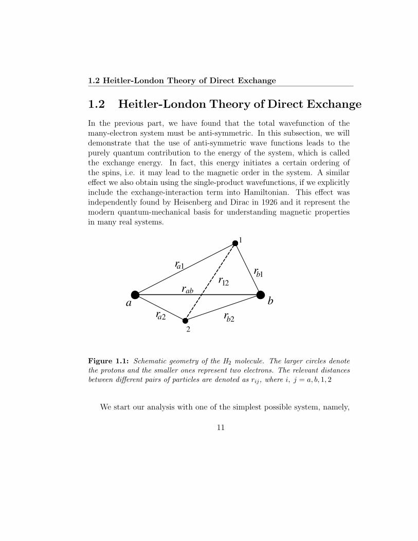
12 Heitler-London Theory of Direct Exchange
12 Heitler-London Theory of Direct Exchange
In the previous part we have found that the total wavefunction of themany-electron system must be anti-symmetric In this subsection we willdemonstrate that the use of anti-symmetric wave functions leads to thepurely quantum contribution to the energy of the system which is calledthe exchange energy In fact this energy initiates a certain ordering ofthe spins ie it may lead to the magnetic order in the system A similareffect we also obtain using the single-product wavefunctions if we explicitlyinclude the exchange-interaction term into Hamiltonian This effect wasindependently found by Heisenberg and Dirac in 1926 and it represent themodern quantum-mechanical basis for understanding magnetic propertiesin many real systems
a b
2
1
r
rrab
r r
ra
a
1
2 2b
21
1b
Figure 11 Schematic geometry of the H2 molecule The larger circles denotethe protons and the smaller ones represent two electrons The relevant distancesbetween different pairs of particles are denoted as rij where i j = a b 1 2
We start our analysis with one of the simplest possible system namely
11
12 Heitler-London Theory of Direct Exchange
H2 molecule In the hydrogen molecule two electrons interact with eachother and with the nuclei of the atoms The situation is schematicallydepicted in Fig11 and considering this geometry we can write the Hamil-tonian of the H2 molecule in the form
H = H1 + H2 + W + HLS (111)
where
H1 = minus ~2
2m∆1 minus
e20ra1
(112)
H2 = minus ~2
2m∆2 minus
e20rb2
(113)
W =e20rab
+e20r12
minus e20rb1
minus e20ra2
(114)
and we have used the abbreviation e0 = e(4πε0) The terms H1 and H2 in(111) describe the situation when the two hydrogen atoms are isolated Theoperator W describes the interaction between two cores electrons as wellas between electrons and relevant nuclei Finally the last term representsthe spin-orbit interaction which is assumed to be small so that we canseparate the orbital and spin degrees of freedom To solve the problem of thehydrogen molecule we apply the first-order perturbation theory neglectingthe spin-orbit coupling and taking the term W as a small perturbationAs it is usual in the perturbation theory we at first solve the unperturbedproblem ie the system of two non-interacting hydrogen atoms Thus wehave to solve the Schrodinger equation
(H1 + H2)Ψ = U0Ψ (115)
12
12 Heitler-London Theory of Direct Exchange
As we already have noted above we will assume that the total wave functioncan be written as a product of the orbital and spin functions ie Ψ =φ(r1 r2)χ(s
z1 s
z2) Another very important point to be emphasized here
is that our simplified Hamiltonian does not explicitly depend on the spinvariables Consequently we can at first evaluate only the problem withorbital functions and at the end of the calculation we can multiply theresult by an appropriate spin function to ensure the anti-symmetry of thetotal wavefunction In order to express this situation mathematically weintroduce the following notations
bull ϕα(ri)where α = a b i = 1 2 represents the orbital wave func-tion of the isolated hydrogen atom when the ith electron is localizedclosely to the αth nucleus
bull ξγ(i)where γ =uarr darr i = 1 2 is the spin function describing thespin up or spin down of the ith electron
Now let us proceed with the discussion of the orbital functions of the systemdescribed by Eq(115) Since the orbital functions ϕα(ri) are eigenfunctionsof the relevant one-atom Schrodinger equation with the same eigenvalueE0 = minus1355 eV it is clear that the ground state of the two noninteractinghydrogen atoms has the energy U0 = 2E0 and it is doubly degeneratedThis is so-called exchange degeneracy and two wavefunctions correspondingto this U0 can be expressed as φ1(r1 r2) = ϕa(r1)ϕb(r2) and φ2(r1 r2) =ϕa(r2)ϕb(r1)
If we include into Hamiltonian also the interaction term W then the sit-uation becomes much more complex and the eigenfunctions and eigenvaluescannot be found exactly In the spirit of the perturbation theory we willassume that the wavefunction of the interacting system can be expressed inthe form
φ(r1 r2) = c1φ1(r1 r2) + c2φ2(r1 r2)
= c1ϕa(r1)ϕb(r2) + c2ϕa(r2)ϕb(r1) (116)
13
12 Heitler-London Theory of Direct Exchange
where c1 and c2 are the constant that will be determined later The systemis now described by the following Schrodinger equation(H1 + H2 + W
)[c1φ1(r1 r2) + c2φ2(r1 r2
]= E
[c1φ1(r1 r2) + c2φ2(r1 r2)
](117)
Multiplying the previous equation by φlowast1(r1 r2) and integrating over the
space one obtains
2c1E0 + 2c2E0
intintφlowast1(r1 r2)φ2(r1 r2)dV1dV2
+ 2c1
intintφlowast1(r1 r2)Wφ1(r1 r2)dV1dV2 + c2
intintφlowast1(r1 r2)Wφ2(r1 r2)dV1dV2
= c1E + c2E
intintφlowast1(r1 r2)φ2(r1 r2)dV1dV2 (118)
Similarly by multiplying Eq(117) by φlowast2(r1 r2) and integrating over the
space one finds
c1E0
intintφlowast2(r1 r2)φ1(r1 r2)dV1dV2 + c1
intintφlowast2(r1 r2)Wφ1(r1 r2)dV1dV2
+ 2c2E0 + c2
intintφlowast2(r1 r2)Wφ2(r1 r2)dV1dV2
= c1E
intintφlowast2(r1 r2)φ1(r1 r2)dV1dV2 + c2E (119)
Here one should notice that in deriving Eqs(118) and (119) we have usednormalization conditions for φ1 and φ2
In order to express two previous equations in an abbreviated form oneintroduces the following quantities
1 The overlap integral
S0 =
intϕlowasta(ri)ϕb(ri)dVi i = 1 2 (120)
14
12 Heitler-London Theory of Direct Exchange
2 The Coulomb integral
K =
intintφlowast1(r1 r2)Wφ1(r1 r2)dV1dV2 =
intintφlowast2(r1 r2)Wφ2(r1 r2)dV1dV2
(121)
3 The exchange integral
A =
intintφlowast1(r1 r2)Wφ2(r1 r2)dV1dV2 =
intintφlowast2(r1 r2)Wφ1(r1 r2)dV1dV2
(122)
Applying this notation we rewrite Eqs(118) and (119) in the form
c1(2E0 +K minus E) + c2(2E0S20 + Aminus ES2
0) = 0
c1(2E0S20 + Aminus ES2
0) + c2(2E0 +K minus E) = 0 (123)
This is a homogeneous set of equations which determines unknown coeffi-cients c1 and c2 Of course we search for non-trivial solutions that can benaturally determined from the equation∣∣∣∣ 2E0 +K minus E 2E0S
20 + Aminus ES2
0
2E0S20 + Aminus ES2
0 2E0 +K minus E
∣∣∣∣ = 0 (124)
From this equation we easily find two possible solutions for the energy Eand the coefficients ci namely
Ea = 2E0 +K minus A
1minus S20
c1 = minusc2 (125)
and
Es = 2E0 +K + A
1 + S20
c1 = c2 (126)
15
12 Heitler-London Theory of Direct Exchange
Finally from the normalization condition of the total wavefunction oneobtains
1 =
int intφlowast(r1 r2)φ(r1 r2)dV1dV2
= 2|c1|2(1∓ S2) (127)
or
c1 =1radic
2(1∓ S20) (128)
where the minus and + sign corresponds to Ea and Es respectively Using(128) we can express the orbital part of the total wavefunctions as
φ(r1 r2) =1radic
2(1minus S20)
[ϕa(r1)ϕb(r2)minus ϕa(r2)ϕb(r1)
](129)
which is clearly the anti-symmetric expression and it corresponds to EaSimilarly the symmetric orbital function which corresponds to Es is givenby
φ(r1 r2) =1radic
2(1 + S20)
[ϕa(r1)ϕb(r2) + ϕa(r2)ϕb(r1)
] (130)
Finally we also can account for the spins of the electrons and to con-struct the following anti-symmetric wavefunctions
Ψ =1radic
2(1minus S20)
∣∣∣∣ ϕa(r1) ϕa(r2)ϕb(r1) ϕb(r2)
∣∣∣∣ ξuarr(1)ξuarr(2) S = 1 Sz = 1 (131)
Ψ =1radic
2(1minus S20)
∣∣∣∣ ϕa(r1) ϕa(r2)ϕb(r1) ϕb(r2)
∣∣∣∣ ξdarr(1)ξdarr(2) S = 1 Sz = 0 (132)
16
12 Heitler-London Theory of Direct Exchange
Ψ =1radic
2(1minus S20)
∣∣∣∣ ϕa(r1) ϕa(r2)ϕb(r1) ϕb(r2)
∣∣∣∣ 1radic2[ξuarr(1)ξdarr(2) + ξdarr(1)ξuarr(2)]
S = 1 Sz = minus1 (133)
and
Ψ =1radic
2(1 + S20)
[ϕa(r1)ϕb(r2) + ϕb(r1)ϕa(r2)
] 1radic2
∣∣∣∣ ξuarr(1) ξuarr(2)ξdarr(1) ξuarr(2)
∣∣∣∣S = 0 Sz = 0 (134)
Here the wavefunctions (131)-(133) form a triplet (threefold degeneratestate) with the energy Ea the total spin S = 1 and the total zth componentSz = plusmn1 0 Similarly the wavefunction (134) describes a singlet state withenergy Es the total spin S = 0 and Sz = 0 Of course both the triplet andsinglet states can be the ground state of the system depending on the signof the exchange integral In order to prove this statement we calculate theenergy difference between Ea and Es ie
∆E = Ea minus Es =2(KS2
0 minus A)
1minus S40
asymp minus2A (135)
where we have neglected the overlap integral which very small in comparisonwith other terms in the expression It is clear from the previous equationthat for A gt 0 the ground state of the system will be represented by thetriplet state with parallel alignment of spins and for A lt 0 the singlet statewith anti-parallel orientation of the spins Of course the parallel (anti-parallel) spin orientation implies also parallel (anti-parallel) alignment of themagnetic moments which is crucial for the observation of the ferromagneticor antiferromagnetic ordering in the real systems
The situation in the hydrogen molecule of course differs from the realsituation in ionic crystal in many respects For example the electrons in
17
12 Heitler-London Theory of Direct Exchange
the hydrogen molecule occupy 1s orbitals while in the ionic crystals theunpaired localized electrons usually occupy d or f orbitals In fact thecalculation of the exchange integral using 3d orbital functions leads to thepositive value of the A Therefore the direct exchange interactions leadsto the ferromagnetic ordering in such systems Later it was discovered byAnderson that the antiferromagnetic ordering is caused by so-called indi-rect exchange interaction via a non-magnetic bridging atom The situationin real materials is usually much more complicated and other mechanismsuch as the Dzyaloshinkii-Moriya or Ruderman-Kittel-Kasuya-Yosida inter-actions can play an important role
Although the calculation performed for the hydrogen molecule does notreflect the complex situation of the real magnetic systems it is extremelyimportant from the methodological point of view In fact it is clear from ourcalculation that the parallel or anti-parallel alignment of the magnetic mo-ments appears due to new contribution to the energy of the system whichoriginates from the indistinguishability of quantum particles The othermechanisms leading to the macroscopic magnetism have also quantum na-ture and cannot be included into the classical theory
Thus we can conclude that the physical origin of magnetism can becorrectly understood and described only within the quantum theory
18
Chapter 2
Bogolyubov Inequality and ItsApplications
21 General Remarks on Bogolyubov Inequal-
ity
The Bogolyubov inequality for the Gibbs free energy G of an interactingmany-body system described by the Hamiltonian H is usually written inthe form
G le G0 + ⟨H minus H0⟩0 = ϕ(λx λy λz ) (21)
In this equation the so-called trial Hamiltonian H0 = H0(λx λy λz )depends on some variational parameters λi that are naturally determinedin the process of calculation and the symbol ⟨ ⟩0 stands for the usualensemble average calculated with the trial Hamiltonian Finally G0 denotesthe Gibbs free energy of the trial system defined by
G0 = G0(λx λy λz ) = minus 1
βlnZ0 (22)
19
22 Mean-Field Theory of Anisotropic Heisenberg Model
where β = 1kBT and the the partition function Z0 is given by
Z0 = Tr eminusβH0 (23)
In general there is a remarkable freedom in defining the trial Hamilto-nian In fact the only limitations to be taken into account follow from thetwo obvious requirements
1 The trial Hamiltonian should naturally represent a simplified physicalmodel of the real system
2 The expression of G0 must be calculated exactly in order to obtain aclosed-form formula for the rhs of Eqs(21)
22 Mean-Field Theory of the Spin-12
Anisotropic Heisenberg Model
221 General Formulation
The accurate theoretical analysis of the Heisenberg model is extremely harddue to interaction terms in the Hamiltonian including non-commutative spinoperators Probably the simplest analytic theory applicable to the modelis the standard mean-field approach Although the mean-field theory canmathematically be formulated in many different ways we will develop in thistext an approach based on the Bogolyubov inequality for the free energy ofthe system The main advantage of this formulation is its completeness (wecan derive analytic formulas for all thermodynamic quantities of interest)and a possibility of further generalizations for example an extension to theOguchi approximation
20
22 Mean-Field Theory of Anisotropic Heisenberg Model
In this part we will study the spin-12 anisotropic Heisenberg model ona crystal lattice described by the Hamiltonian
H = minussumij
(JxSxi S
xj + JyS
yi S
yj + JzS
zi S
zj )minus gmicroB
sumi
(HxSxi +HyS
yi +HzS
zi )
(24)where g is the Lande factor microB is the Bohr magneton Jα and Hα α =x y z denote the spatial components of the exchange interaction and exter-nal magnetic field respectively One should note here that Jα is assumedto be positive for the ferromagnetic systems and negative for the antifer-romagnetic ones Moreover it is well-known that the absolute value ofexchange integrals very rapidly decreases with the distance thus we canrestrict the summation in the first term of (24) to the nearest-neighboringpairs of atoms on the lattice Finally the spatial components of the spin-12operators are given by
Sxk =
1
2
(0 11 0
)k
Syk =
1
2
(0 minusii 0
)k
Szk =
1
2
(1 00 minus1
)k
(25)
To proceed further we choose the trial Hamiltonian in the form
H0 = minusNsumk
(λxS
xk + λyS
yk + λzS
zk
) (26)
where N denotes the total number of the lattice sites and λi are variationalparameters to be determined be minimizing of the rhs of the Bogolyubovinequality After substituting (25) into (26) we can apparently rewriteprevious equation as follows
H0 =Nsumk=1
H0k (27)
21
22 Mean-Field Theory of Anisotropic Heisenberg Model
where the site Hamiltonian H0k is given by
H0k = minus1
2
(λz λx minus iλy
λx + iλy minusλz
)k
(28)
In order to evaluate the terms entering the Bogolyubov inequality we atfirst have to calculate the partition function Z0 Taking into account thecommutation relation [H0k H0ℓ] = 0 for k = ℓ we obtain the followingexpression
Z0 = Tr exp(minusβ
Nsumk=1
H0k
)=
Nprodk=1
Trk exp(minusβH0k
) (29)
where Trk denotes the trace of the relevant operator related to kth latticesite Now after setting Eq(28) into (29) one obtains
Z0 =Nprodk=1
Trk exp
(β2λz
β2(λx minus iλy)
β2(λx + iλy) minusβ
2λz
)k
=
[Trk exp
(β2λz
β2(λx minus iλy)
β2(λx + iλy) minusβ
2λz
)k
]N
(210)
The crucial point for further calculation is the evaluation of exponentialfunction in previous equation Let us note that in performing this task wewill not follow the usual approach based on the diagonalization of modifiedmatrix (28) entering the argument of exponential Instead we will performall calculations in the real space by applying the following matrix form ofthe Cauchy integral formula
eminusβH0k =1
2πi
∮C
ezdz
zI minus (minusβH0k) (211)
22
22 Mean-Field Theory of Anisotropic Heisenberg Model
After a straightforward calculation we obtain
eminusβH0k =
(h11 h12
h21 h22
)(212)
with
h11 = cosh
(β
2Λ
)+
λz
Λsinh
(β
2Λ
)(213)
h12 =λx minus iλy
Λsinh
(β
2Λ
)(214)
h21 =λx + iλy
Λsinh
(β
2Λ
)(215)
h22 = cosh
(β
2Λ
)minus λz
Λsinh
(β
2Λ
) (216)
where we have introduced the parameter
Λ =radicλ2x + λ2
y + λ2z (217)
Using previous equations we easily obtain the following expressions for Z0
and G0
Z0 =
[2 cosh
(β
2Λ
)]N(218)
G0 = minusN
βln
[2 cosh
(β2Λ
)] (219)
23
22 Mean-Field Theory of Anisotropic Heisenberg Model
To obtain the complete expression for ϕ(λx λy λz ) we have to eval-
uate the terms ⟨H⟩0 and ⟨H0⟩0 that can be expressed as
⟨H⟩0 = minusNq
2
(Jx⟨Sx
i Sxj ⟩0 + Jy⟨Sy
i Syj ⟩0 + Jz⟨Sz
i Szj ⟩0
)minus N
(hx⟨Sx
j ⟩0 + hy⟨Syj ⟩0 + hz⟨Sz
j ⟩0) (220)
where q denotes the coordination number of the lattice and hα = gmicroBHα(α = x y z) Similarly we have
⟨H0⟩0 = minusN(λx⟨Sx
j ⟩0 + λy⟨Syj ⟩0 + λz⟨Sz
j ⟩0) (221)
The ensemble averages of ⟨Sαj ⟩0 entering two previous equations can be
expressed in the form
⟨Sαj ⟩0 =
1
Z0
TrSαj e
minusβH0
=TrjS
αj exp
(minusβH0j
)prodNminus1k =j Trk exp
(minusβH0k
)Trj exp
(minusβH0j
)prodNminus1k =j Trk exp
(minusβH0k
) (222)
which can be simplified as follows
⟨Sαj ⟩0 =
TrjSαj exp
(minusβH0j
)Trj exp
(minusβH0j
) (223)
Similarly one easily finds that
⟨Sαi S
αj ⟩0 =
TriSαi exp
(minusβH0i
)Tri exp
(minusβH0i
) TrjSαj exp
(minusβH0j
)Trj exp
(minusβH0j
) =(⟨Sα
j ⟩0)2
(224)
24
22 Mean-Field Theory of Anisotropic Heisenberg Model
In order to complete our calculation we substitute Eqs (212)-(216) intoEq (223) and then we evaluate the trace of relevant matrices In this waywe obtain the following equation
⟨Sαj ⟩0 =
λα
2Λtanh
(β
2Λ
) (225)
and
⟨Sαi S
αj ⟩0 =
(λα
2Λ
)2
tanh2
(β
2Λ
) (226)
After introducing notation ⟨Sαj ⟩0 = mα α = x y z we can rewrite the rhs
of the Bogolyubov inequality in the form
ϕ(λx λy λz) = minusN
βln(2 cosh
β
2Λ)minus Nq
2
(Jxm
2x + Jym
2y + Jzm
2z
)+ N
[(λx minus hx)mx + (λy minus hy)my + (λz minus hz)mz
] (227)
Since the quantity ϕ represents an upper bound for the exact Gibbs freeenergy of the system then the best possible approximation (with the trialHamiltonian H0) corresponds for those values of λx λy λz that minimizeϕ(λx λy λz) Relevant values of λx λy λz are obviously determined fromthe equations
partϕ
partλx
= 0partϕ
partλy
= 0partϕ
partλz
= 0 (228)
The above conditions lead to three independent equations that can berewritten in the following simple matrix form
partmx
partλx
partmy
partλx
partmz
partλxpartmx
partλy
partmy
partλy
partmz
partλy
partmx
partλz
partmy
partλz
partmz
partλz
λx minus qJxmx minus hx
λy minus qJymy minus hy
λz minus qJzmz minus hz
= 0 (229)
25
22 Mean-Field Theory of Anisotropic Heisenberg Model
Since the first matrix in (229) is in general non-zero then the only possiblesolution of this equation is given by
λx = qJxmx + hx λy = qJymy + hy λz = qJzmz + hz (230)
and the cooresponding equilibrium Gibbs free energy can be after a smallmanipulation expressed in the form
G = minusN
βln2 cosh
(βhef
2
)+
Nq
2
(Jxm
2x + Jym
2y + Jzm
2z
) (231)
where we have denoted
hef =radic
(qJxmx + hx)2 + (qJymy + hy)2 + (qJzmz + hz)2 (232)
Having obtained the last equation we are able to identify the physicalmeaning of the parameters mxmymx and consequently also the meaningof variational parameters λx λy λz
For this purpose we at first recall that the spatial component of thetotal magnetization Mα is defined as
Mα = minus(
partGpartHα
)β
= minusgmicroB
(partGparthα
)β
(233)
After a straightforward calculation we obtain the following very simple ex-pressions
Mx
NgmicroB
= mx = ⟨Sxj ⟩0
My
NgmicroB
= my = ⟨Syj ⟩0
Mz
NgmicroB
= mz = ⟨Szj ⟩0
(234)
which clearly indicate that mα represents the spatial components of themagnetization Consequently the parameters λα have the meaning of ofthe molecular-field components acting on one atom in the lattice Thusour formulation is nothing but the standard mean-field theory The mainadvantage of our approach is that this formulation provides a close-form an-alytical expression for the Gibbs free energy which is of principal importancefor finding stability conditions of various physical quantities
26
22 Mean-Field Theory of Anisotropic Heisenberg Model
222 Thermodynamic Properties of the HeisenbergModel
Now let us proceed with the calculation of several interesting physical quan-tities for the system under investigation Using Eqs (222) (230) and(234) one simply obtains for the components of reduced magnetization aset of three coupled equations namely
mx =qJxmx + hx
2hef
tanh
(β
2hef
) (235)
my =qJymy + hy
2hef
tanh
(β
2hef
) (236)
mz =qJzmz + hz
2hef
tanh
(β
2hef
) (237)
where we have denotedIn order to investigate the long-range ordering the systems we set hx =
hy = hz = 0 and obtain
mx =Jxmx
2h0
tanh
(βq
2h0
) (238)
my =Jymy
2h0
tanh
(βq
2h0
) (239)
mz =Jzmz
2h0
tanh
(βq
2h0
) (240)
27
22 Mean-Field Theory of Anisotropic Heisenberg Model
with
h0 =radic(Jxmx)2 + (Jymy)2 + (Jzmz)2 (241)
These three nonlinear equations have always the trivial solution mx =my = mz = 0 corresponding to the disordered paramagnetic phase (DP)Moreover depending on the temperature and the values of exchange pa-rameters there also exist non-trivial solutions corresponding to ordered fer-romagnetic phase (OP) The stability of the relevant solutions is then de-termined by the minimum of the Gibbs free energy given by Eq(231) Nowwe briefly analyze possible trivial and non-trivial solutions of (238)-(240)for some particular cases of the exchange interactions
1 Ising model Jx = Jy = 0 Jz = J = 0
mx = my = 0 and mz =1
2tanh
(qβJ2
mz
)for T lt Tc
mx = my = mz = 0 for T gt Tc (242)
2 Isotropic XY model Jx = Jy = J = 0 Jz = 0
mz = 0my = mx and mx =1
2radic2tanh
(radic2qβJ
2mx
)for T lt Tc
mx = my = mz = 0 for T gt Tc (243)
3 Isotropic Heisenberg model Jx = Jy = Jz = 0
my = mx = mz and mz =1
2radic3tanh
(radic3qβJx2
mx
)for T lt Tc
mx = my = mz = 0 for T gt Tc (244)
28
22 Mean-Field Theory of Anisotropic Heisenberg Model
Here one should note that non-trivial results for isotropic XY and Heisen-berg model model represents valid solution for the models when the axis ofquantization is given by the equation y = x = t t isin R for the XY modeland y = x = z = t t isin R for the Heisenberg model On the other handif choose as a quantization axis for example the x axis then we obtain forboth models identical result as that for the Ising one Thus one can concludethat mean-field theory is not able to describe correctly quantum featuresof localized spin models In order to illustrate the numerical accuracy ofthe method we have compared in Fig 23 the temperature variation of themean-field magnetization with exact result on the square lattice with q = 4
00 05 10 15000
025
050q = 4
m
kBT J
Exact
MFT
Figure 21 Comparisom of the temperature dependence of magnetization forthe Ising model on a square lattice
The critical (or Curie) temperature is defined as a temperature at whichthe long-range order (or magnetization) vanishes In order to determine the
29
22 Mean-Field Theory of Anisotropic Heisenberg Model
Curie temperature we take into account that tanh(x) asymp x for x ltlt 1 andobtain an universal solution
Tc =qJα
4kB α = x y z (245)
which valid for all three cases mentioned above Of course the critical tem-perature should be different depending on the model considered Thus thepresent method is not able to distinguish specific features of the models aslong as concerns the critical behavior Moreover it is also clear that thetopology of the lattice is taken into account only through its coordinationnumber that is also weak point of the present method It is well knownthat this approach significantly fails for the low-dimensional systems nev-ertheless it gives rather good qualitative picture for the three-dimensionalsystems and therefore it is frequently used to obtain analytical results par-ticularly for complex systems
Finally one should note that calculations of other thermodynamic quan-tities is easy and straightforward since we have analytical solution for theGibbs free energy of the system from which other quantities are easily ob-tained
This calculation including numerical analysis and discussion is left forthe readers as an appropriate exercise
Let us conclude this part by noticing that the present approach can beextended to case of the the so-called Oguchi approximation which alreadyaccount much better for the quantum effects as well as for the spin-spincorrelations Possible extensions are rather involved and require lengthycalculations that are beyond the scope of the present book
30
Chapter 3
Spin-Wave Theory
31 Bloch Spin-Wave Theory of Ferromag-
nets
In this part we will discuss the concept of spin waves which enables to studythe some physical properties of magnetic systems at low temperatures Thistheory was originally introduced by F Bloch [1] and its main assumptionis that the ground state of the system is ordered and the excited states aredescribed as a collection of spin waves At low temperatures it is reasonableto expect the small amplitudes of the spin waves thus the interaction amongspin waves can be neglected We will consider in this part an isotropicHeisenberg model defined by the Hamiltonian
H = minusJsumij
SiSj minus gmicroBHsumi
Szi (31)
Here Si represents a vector spin-operator at the ith site of the lattice Thisoperator is naturally defined as Si = (Sx
i Syi S
zi ) where Sα
i (α = x y z)represent spatial components of the standard spin operators g is the Lande
31
31 Bloch Spin-Wave Theory of Ferromagnets
factor microB is the Bohr magneton and H denotes the external magnetic fieldwhich is applied along z axis J is the exchange integral which is assumedto be positive since we are going to investigate the ferromagnetic systems
Adopting the basic concept of lattice vibrations we can write the fol-lowing equation of motion of the spin Sℓ on the j th lattice point
dSℓ
dt=
i
~[H Sℓ] (32)
In what follows we will use the following commutation relations for spinoperators
[Sai S
bj ] = iεabcδijS
cj a b c = x y or z (33)
where εabc represents Levi-Civita tensor and δij is the Kronecker symbolNow substituting the Hamiltonian (31) into (32) and employing relations(33) one obtains
dSℓ
dt= minus1
~(Hℓ times Sℓ) (34)
where the local magnetic field Hℓ acting on the j th spin is given by
Hℓ =sumj
JjℓSj + gmicroBHe3 (35)
with e3 = (0 0 1) Using two previous equations one easily obtains thefollowing equations of motion of the x y and z components of the spinoperator
~dSx
ℓ
dt= minus
sumj
Jjℓ(Syj S
zℓ minus Sz
j Syℓ ) + gmicroBHSy
ℓ (36)
~dSy
ℓ
dt= minus
sumj
Jjℓ(Szj S
xℓ minus Sx
j Szℓ )minus gmicroBHSx
ℓ (37)
32
31 Bloch Spin-Wave Theory of Ferromagnets
~dSz
ℓ
dt= minus
sumj
Jjℓ(Sxj S
yℓ minus Sy
j Sxℓ ) (38)
If we restrict ourselves to the case of low-energy excitation then the compo-nents Sx
ℓ Syℓ can be regarded as small quantities of first order Consequently
the right-hand side of (38) is a small quantity of the second order whichcan be neglected and it follows from Eq (38) that the zth component be-comes a constant Moreover it is reasonable to put explicitly Sz
ℓ = S sincethe external magnetic field is assumed to be applied parallel to the zth axisUnder these assumptions Eqs (36) and (37) can be rewritten in the form
~dSx
ℓ
dt= minusS
sumj
Jjℓ(Syj minus Sy
ℓ ) + gmicroBHSyℓ (39)
~dSy
ℓ
dt= minusS
sumj
Jjℓ(Sxℓ minus Sx
j )minus gmicroBHSxℓ (310)
or alternatively
~dS+
ℓ
dt= minusiS
sumj
Jjℓ(S+ℓ minus S+
j )minus gmicroBHS+ℓ (311)
~dSminus
ℓ
dt= minusiS
sumj
Jjℓ(Sminusℓ minus Sminus
j )minus gmicroBHSminusℓ (312)
where we have introduced the spin-raising and spin-lowering operators
S+ℓ = Sx
ℓ + iSyℓ Sminus
ℓ = Sxℓ minus iSy
ℓ (313)
that obey the following commutation rules
[Szk S
+ℓ ] = S+
k δkℓ [Szk S
minusℓ ] = minusSminus
k δkℓ [S+k S
+ℓ ] = 2Sz
kδkℓ (314)
33
31 Bloch Spin-Wave Theory of Ferromagnets
The above relations are directly obtained with the help of well-known com-mutation relations of the spin operators (33)
To proceed further we now express the spin-raising and spin-loweringoperators with the help of the Fourier transform ie
S+q =
1radicN
sumj
eiqmiddotRj S+j Sminus
q =1radicN
sumj
eminusiqmiddotRj Sminusj (315)
S+j =
1radicN
sumq
eminusiqmiddotRj Sq Sminusj =
1radicN
sumq
eiqmiddotRj Sq (316)
Substituting Eq(316) into Eq(312) and applying the following relationsumℓ
eminusi(q1minusq2)middotRℓ = Nδq1q2 (317)
one gets equation
minusi~dSminus
q
dt=
[Ssumℓ
Jjℓ(1minus eminusiqmiddot(RjminusRℓ)) + gmicroBH]Sminusq (318)
If we now introduce a real quantity
J(q) =sumj
J(Rj)eminusiqmiddotRj (319)
then we rewrite (318) as
minusi~dSminus
q
dt=
S[J(0)minus J(q)
]+ gmicroBH
Sminusq (320)
It is straightforward to obtain the solution of this equation in the form
Sq = δSqei(ωqt+α) (321)
34
31 Bloch Spin-Wave Theory of Ferromagnets
where the eigenfrequencies of the spin waves are given by
~ωq = S[J(0)minus J(q)
]+ gmicroBH (322)
One should notice here that in the limit of small q we obtain ~ωq asymp q2Now using Eq(321) we can express the spin operators in the real space
as follows
Sminusj =
1radicNδSqe
i(qmiddotRj+ωqt+α) (323)
Sxj =
1radicNδSq cos
[i(q middotRj + ωqt+ α)
](324)
and
Syj = minus 1radic
NδSq sin
[i(q middotRj + ωqt+ α)
] (325)
Finally it is straightforward to prove that the energy difference betweenan excited state and ground state is given by
Eq minus E0 = ~ωq (326)
where ~ωq represents the excitation energy of the spin wave with the wavevec-tor q The proof of the last statement is left as an appropriate exercise forreaders
35
32 Holstein-Primakoff theory of ferromagnets
32 Holstein-Primakoff theory of ferromag-
nets
The Blochrsquos spin-wave theory discussed in previous chapter represents a verysimple approach in which we completely neglect the interaction among spinwaves This deficiency can be eliminated using an alternative formulationbased on magnon variables (or creation-annihilation operators) developedby Holstein and Primakoff [2] In this part we apply The Holstein-Primakofftheory to case of an anisotropic quantum Heisenberg model described bythe Hamiltonian
H = minusJsumij
(Sxi S
xj + Sy
i Syj + Sz
i Szj )minus gmicroBH
sumi
Szi (327)
The meaning of all symbols in previous Eq (327) is the same as in previoustext
In order to apply a spin-wave picture to analyze magnetic properties ofthe model under investigation one has to perform three subsequent math-ematical transformation At first we express the components of the spinoperators trough spin-lowering and spin raising operators then we intro-duce so-called creation and annihilation operators and finally we performa Fourier transform of the relevant all creation and annihilation operatorsentering the Hamiltonian The eigenvalues of the final Hamiltonian then en-able to determine relevant physical quantities applying standard relationsof statistical mechanics For further manipulations it is more convenient torewrite (327) as follows
H = minusJsumℓδ
(Sxℓ S
xℓ+δ + Sy
ℓ Syℓ+δ + Sz
ℓ Szℓ+δ)minus gmicroBH
sumℓ
Szℓ (328)
where ℓ labels the lattice sites and δ denotes nearest neighbors of the relevantsite and we assume that J gt 0 The integrals of motion for Hamiltonian
36
32 Holstein-Primakoff theory of ferromagnets
(328) are the total z th component Sz =sum
k Szk and the total spin of the
systemThe ground state of the system is ordered and for H gt 0 the magnetic
moment is paralell to the z axis If we consider the lattice consisting of Natoms with spin S then the ground-state vector in the spin basis reads |0⟩= |NSNS⟩ Of course we work in a real space basis in which the spinoperators Sz
ℓ are diagonal We recall that the eigenvalues MS = minusS minusS +1 S and eigenvectors |MS⟩ℓ of the operator Sz
ℓ satisfy the followingequation
Szℓ |MS⟩ℓ = MS|MS⟩ℓ (329)
Now applying operators (313) to the eigenvectors |MS⟩ℓ one obtains
S+ℓ |MS⟩ℓ =
radic(S minusMS)(S minusMS minus 1)|MS + 1⟩ℓ (330)
and
Sminusℓ |MS⟩ℓ =
radic(S +MS)(S minusMS minus 1)|MS minus 1⟩ℓ (331)
In addition to the spin-raising and spin-lowering operators we will alsouse in our analysis the operator describing a deviation of the zth spin-component from its maximum value namely
nℓ = S minus Szℓ (332)
The eigenvalues of this operator are integers nl = 0 1 2 2S (or nl =S minusMS) thus we can rewrite Eqs(330) in the form
S+ℓ |nℓ⟩ℓ =
radic2S
radic1minus (nℓ minus 1)
2S
radicnℓ|nℓ minus 1⟩ℓ (333)
Le us note that performing a similar procedure is also possible for Eq(331)and it will be used later
37
32 Holstein-Primakoff theory of ferromagnets
Now with the help of (313) we can rewrite the Hamiltonian (328) inthe form
H = minusJsumℓδ
[12(S+
ℓ Sminusℓ+δ + Sminus
ℓ S+ℓ+δ) + Sz
ℓ Szℓ+δ
]minus gmicroBH
sumℓ
Szℓ (334)
which is suitable for introducing the Holstein-Primakoff magnon represen-tation In order to define the relevant transformation we at first introducethe standard creation and annihilation operators that are defined as
adaggerℓΨnℓ=
radicnℓ + 1Ψnℓ+1 aℓΨnℓ
=radicnℓΨnℓminus1 (335)
The central idea of the Holstein-Primakoff approach is based on the intro-duction of the following transformation
S+ℓ = (2S)12
(1minus adaggerℓaℓ
2S
)12
aℓ (336)
Sminusℓ = (2S)12adaggerℓ
(1minus adaggerℓaℓ
2S
)12
(337)
Szℓ = S minus adaggerℓaℓ (338)
As already noted above the eigenvalues of adaggerℓaℓ are arbitrary integers whilethat of nℓ are limited to the range 0 le nℓ le 2S Fortunately this discrep-ancy does not play any important role in the calculation since the transitionfrom the state with nℓ le 2S to states with nℓ gt 2S never occur eg
Sminusℓ Ψ2S = (2S)12(2S + 1)12
(1minus 2S
2S
)12
Ψ2S+1 = 0 (339)
Now we transform the operators aℓ adaggerℓ from the real space to the reciprocal
space by the following Fourier tansform
aℓ =1radicN
sumq
eminusiqmiddotRℓbq (340)
38
32 Holstein-Primakoff theory of ferromagnets
adaggerℓ =1radicN
sumq
eiqmiddotRℓbdaggerq (341)
where N denotes the total number of atoms q represents a vector of thereciprocal space and Rℓ represents a vector specifying the position of ℓthatom in the lattice
The magnon-annihilation and magnon-creation operators are given by
bq =1radicN
sumℓ
eiqmiddotRℓaℓ (342)
bdaggerq =1radicN
sumℓ
eminusiqmiddotRℓadaggerℓ (343)
and they obey the usual magnon commutation relations
[bq1 bdaggerq2] = δq1q2 [bq1 bq2 ] = [bdaggerq1
bdaggerq2] = 0 (344)
It is useful to note here that the operator bdaggerq creates a magnon with thewave vector q and the operator bq annihilates it Moreover it follows fromthe transformation (340) and (341) that any change of the spin state atarbitrary lattice site is described as a superposition of an infinite number ofthe spin waves
At this stage it is clear that further exact treatment of the problem isimpossible due to the complexity of applied transformations The progressis however still possible if we restrict ourselves to the case when the numberof excited states is small in comparison with 2S Under this assumptionwe can neglect the higher order terms in expansion of the square root andrewrite Eqs (336) and (337) in the form
S+ℓ = (2S)12
(1minus adaggerℓaℓ
4S
)aℓ + (345)
39
32 Holstein-Primakoff theory of ferromagnets
Sminusℓ = (2S)12adaggerℓ
(1minus adaggerℓaℓ
4S
)+ (346)
Finally substituting (340) and (341) into previous equation one obtains
S+ℓ =
(2S
N
)12[sumq1
eminusiq1middotRℓbq1 minus1
4SN
sumq1q2q3
ei(q1minusq2minusq3)middotRℓbdaggerq1bq2bq3 +
](347)
Sminusℓ =
(2S
N
)12[sumq1
eiq1middotRℓbdaggerq1minus 1
4SN
sumq1q2q3
ei(q1+q2minusq3)middotRℓbdaggerq1bdaggerq2
bq3 +
](348)
Similarly the operator Szℓ is given by
Szℓ = S minus 1
N
sumq1q2
ei(q1minusq2)middotRℓbdaggerq1bq2 (349)
If we assume that each lattice site has z nearest neighbors then we canspecify their positions on the lattice by introducing the vector
δ = Rℓ+δ minusRℓ (350)
Substituting (347)-(350) into Eq(334) and performing a rearrange-ment of the terms one can rewrite the Hamiltonian as
H = minusJNzS2 minus gmicroBNHS + H0 + H1 (351)
where H0 is a bilinear form in the magnon variables and it is given by
H0 = minus JS
N
sumℓδ
sumq1q2
[eminusi(q1minusq2)middotRℓeiq2middotδbq1b
daggerq2
+ ei(q1minusq2)middotRℓeminusiq2middotδbdaggerq1bq2
]+
JS
N
sumℓδ
sumq1q2
[ei(q1minusq2)middotRℓbq1b
daggerq2
+ eminusi(q1minusq2)middotRℓei(q1minusq2)middotδbdaggerq1bq2
]+
gmicroBH
N
sumℓq1q2
ei(q1minusq2)middotRℓbdaggerq1bq2 (352)
40
32 Holstein-Primakoff theory of ferromagnets
The term H1 includes higher-order terms and for the sake of simplicity willbe neglected Now taking into account the relation (317) and performingthe summation over ℓ and q2 we can simplify Eq(352) as follows
H0 = minusJzSsumq
(γqbqbdaggerq + γminusqb
daggerqbq minus 2bdaggerqbq) + gmicroBH
sumq
bdaggerqbq (353)
where
γq =1
z
sumδ
eiqmiddotδ (354)
and the summation in (354) runs over all nearest neighbors For furthermanipulation it useful noticing that
sumq γq = 0 and moreover for the crys-
tals with the symmetry center we have γq = γminusk Employing the magnoncommutation rules [bdaggerqbq] = 1 one obtains
H0 =sumq
[2JzS(1minus γq) + gmicroBH
]bdaggerqbq (355)
The last equation can be rewritten in the following very simple form
H0 =sumq
~ωqnq (356)
where nq is the magnon occupation operator and
~ωq = 2JzS(1minus γq) + gmicroBH (357)
Since the quantity γq can be expressed as follows
γq =1
z
sumδ
eiqmiddotδ =1
2z
sumδ
(eiqmiddotδ + eminusiqmiddotδ) =1
2z
sumδ
cos(q middot δ) (358)
then the dispersion relation becomes
~ωq = 2JzS[1minus 1
2z
sumδ
cos(q middot δ)]+ gmicroBH (359)
41
32 Holstein-Primakoff theory of ferromagnets
321 Internal Energy and Specific heat
In this subsection we will show how one can calculate the internal energyand specific heat of Heisenberg model within the Holstein-Primakoff theoryBefore performing any calculation it is useful noticing that due to neglectinghigher order terms in Eq (345) and (346) we treat the ensemble of non-interacting magnons In further calculatiuon we also will assume H = 0and |q middot δ| ≪ 1
Under these assumptions the internal energy of the magnon gas in ther-modynamic equilibrium at temperature T can be expressed as
U =sumq
~ωq⟨nq⟩ (360)
where ⟨nq⟩ is given by the well-known Bose-Einstein relation
⟨nq⟩ =[exp
( ~ωq
kBT
)minus 1
]minus1
(361)
Substituting (361) into (360) one gets
U =sumq
~ωq
[exp
( ~ωq
kBT
)minus 1
]minus1
=1
(2π)3
intDq2
[exp
(Dq2
kBT
)minus 1
]minus1
d3q
=1
2π2
intDq4
[exp
(Dq2
kBT
)minus 1
]minus1
dq (362)
where we have introduced the lattice stiffnes as D = 2SJa2 If we denotex = Dq2kBT then we can rewrite (362) as
U =(kBT )
52
4π2D32
int xm
0
x32
exp(x)minus 1dx (363)
42
32 Holstein-Primakoff theory of ferromagnets
The last expression can be further simplified by considering the regionkBT ≪ ωmax Then the upper limit in the integral (363) can be approxi-mated by infinity and one obtains for internal energy the following analyticalexpression for internal energy of the system
U =(kBT )
52
4π2D32Γ(52
)ζ(52 1) (364)
Here Γ and ζ denote the Gamma- and Riemann zeta-functions respectively
and their numerical values of relevant arguments are known to be Γ(
52
)=
3radicπ
4and ζ
(52 1)= 1341
Thus we finally obtain
U ≃ 045(kBT )52
π2D32 (365)
Consequently for the magnetic part of specific heat at constant volume isgiven by
CV = 0113kB
(kBTD
) 32 (366)
In this work we consider strictly insulating materials thus there is no elec-tron contribution to the total specific heat Consequently taking into ac-count the phonon and magnon contribution we can express the total specificheat at low temperatures by the formula
C = aT 3 + bT 32 (367)
It is clear from this equation that the magnon contribution can experimen-tally easily determined if we plot the dependence of reduced specific heatCT 32 versus T 32 The situation is schematically illustrated in Fig 31
43
32 Holstein-Primakoff theory of ferromagnets
0 2 4 6 80
1
2
CT -32
T 32
magnoncontribution
Figure 31 The re-scaled specific heat vs T 32
322 Magnetization and Critical Temperature
The magnetic moment of the system can be calculated from the equation
MS = gmicroB
⟨(NS minus
sumq
bdaggerqbq)⟩ (368)
The deviation of the magnetization from its saturation value can be ex-pressed as
∆M = M(0)minusM(T ) = gmicroB
sumq
⟨nq⟩
=gmicroB
(2π)3
int qm
0
[exp
(Dq2
kBT
)minus 1
]minus1
d3q (369)
44
33 Holstein-Primakoff theory of antiferromagnets
At low temperatures (Dq2 ≫ kBTJ) we obtain
∆M =gmicroB
2π2
(kBTJD
)32int infin
0
x12
exp(x)minus 1dx
=gmicroB
2π2
(kBTJD
)32
Γ(52
)ζ(32 1)
= 0117gmicroB
(kBTD
)32
(370)
The finite-temperature magnetization can be then expressed as
M(T ) = M(0)[1minus
( T
Tc
) 32]
(371)
where the critical temperature Tc is given by
Tc =( M(0)
0117gmicroB
) 23 D
kB (372)
33 Holstein-Primakoff theory of antiferro-
magnets
The Holstein-Primakoff theory can be extended also to the case of antifero-magnetic Heisenberg model which can describe many real materials [7] Onthe other hand the generalization of the Holstein-Primakoff for quantumantiferromagnets is very interesting because such systems exhibit very inter-esting magnetic properties that differ from quantum ferromagnets in manyrespects Our aim in this subsection is to investigate the antiferromagneticHeisenberg model spin system consisting of two interpenetrating sublatticesa and b which is described by the Hamiltonian
H = minusJsumij
SaiSbj minus gmicroBHa
sumi
Szai + gmicroBHa
sumj
Szbj (373)
45
33 Holstein-Primakoff theory of antiferromagnets
where J lt 0 is the exchange interaction which couples the nearest neighborson lattice and the quantity Ha gt 0 represents an external magnetic fieldwhich is parallel to the z axis In what follows we will treat the problem ap-plying the Holstein-Primakoff transformation for each sublattice separatelyAt first we express the spin rising and lowering sublattice operators withthe help of creation-annihilation operators as follows
S+aj = (2S)12
(1minus
adaggerjaj
2S
)12
aj Sminusaj = (2S)12adaggerj
(1minus
adaggerjaj
2S
)12
(374)
S+bℓ = (2S)12
(1minus bdaggerℓbℓ
2S
)12
bℓ Sminusbℓ = (2S)12bdaggerℓ
(1minus bdaggerℓbℓ
2S
)12
(375)
Szaj = S minus adaggerjaj minusSz
bℓ = S minus bdaggerℓbℓ (376)
Next we introduce the sublattice spin-wave variables
cq =2radicN
sumj
eminusiqmiddotRjaj cdaggerq =2radicN
sumj
eiqmiddotRjadaggerj (377)
dq =2radicN
sumℓ
eiqmiddotRℓbℓ ddaggerq =2radicN
sumℓ
eminusiqmiddotRℓbdaggerℓ (378)
In previous equations summations run over all N atoms of the a and b sub-lattice respectively Moreover the following magnon commutation relationshold
[cq1 cdaggerq2] = [dq1 d
daggerq2] = δq1q2
[cq1 cq2 ] = [cdaggerq1 cdaggerq2
] = 0 [dq1 dq2 ] = [ddaggerq1 ddaggerq2
] = 0 (379)
46
33 Holstein-Primakoff theory of antiferromagnets
Now we expand (374)-(375) as
S+aj =
(4S
N
)12[sumq1
eminusiq1middotRjcq1 minus1
8SN
sumq1q2q3
ei(q1minusq2minusq3)middotRjcdaggerq1cq2cq3 +
](380)
Sminusaj =
(4S
N
)12[sumq1
eiq1middotRjcdaggerq1minus 1
8SN
sumq1q2q3
ei(q1+q2minusq3)middotRjcdaggerq1cdaggerq2
cq3 +
](381)
S+bℓ =
(4S
N
)12[sumq1
eminusiq1middotRℓdq1 minus1
8SN
sumq1q2q3
ei(q1minusq2minusq3)middotRℓddaggerq1dq2dq3 +
](382)
Sminusbℓ =
(4S
N
)12[sumq1
eiq1middotRℓddaggerq1minus 1
8SN
sumq1q2q3
ei(q1+q2minusq3)middotRℓddaggerq1ddaggerq2
dq3 +
](383)
Szaj = S minus 1
N
sumq1q2
ei(q1minusq2)Rjcdaggerq1cq2 (384)
Szbℓ = minusS +
1
N
sumq1q2
eminusi(q1minusq2)Rℓddaggerq1dq2 (385)
Substituting these expansions into (373) and using (317) we obtain
H = NzJS2 + H0 + H1 (386)
47
33 Holstein-Primakoff theory of antiferromagnets
where H0 is a part of the Hamiltonian which is bilinear in magnon variablesie
H0 = minus2JzSsumq
[γq(cdaggerqd
daggerq + cqdq
)+(cdaggerqcq + ddaggerqdq
)]+ gmicroBH
sumq
(cdaggerqcq minus ddaggerqdq
)(387)
where γq is given by (354) and the existence of symmetry center of the
lattice has been assumed The quantity H1 includes higher-order termsand will be for the simplicity neglected However even after neglectingH1 the energy spectrum of system cannot be simply obtained since theHamiltonian is not yet diagonal Thus the main problem to be solved is thediagonalization of H0 In order to make a progress we introduce here newset of the creation and annihilation operators αdagger
q αq βdaggerq βq
αq = uqcq minus vqddaggerq αdagger
q = uqcdaggerq minus vqdq (388)
βq = uqdq minus vqcdaggerq βdagger
q = uqddaggerq minus vqcq (389)
obeying the following commutation rules
[αq αdaggerq] = 1 [βk β
daggerq] = 1 [αq βq] = 0 (390)
The real quantities entering previous equations satisfy relation
u2q minus v2q = 1 (391)
and the inverse transformation are given by
cq = uqαq minus vqβdaggerq cdaggerq = uqα
daggerq minus vqβq (392)
dq = uqβq minus vqαdaggerq ddaggerq = uqβ
daggerq minus vqαq (393)
48
33 Holstein-Primakoff theory of antiferromagnets
The parameters uq and vq in transformations (392) and (393) can be de-termined explicitly in the form
uq = cosh θq vq = sinh θq (394)
where θq is given by
tanh(2θq) = γq (395)
The explicit forms of the transformation given by (394) and (395) is usuallycalled in the literature as Bogolyubov transformation Substituting (392)and (393) into (387) one finally obtains for H the folloving simple relation
H = NJzS(S + 1) +sumq
[~ω+
q
(αdaggerqαq +
1
2
)+ ~ωminus
q
(βdaggerqβq +
1
2
)](396)
where we have defined the eigenfrequencies of the system as
~ωplusmnq = minus2JzS
radic1minus γ2
q plusmn gmicroBH (397)
331 Ground-State Energy
In this part we investigate the ground-state energy of the two sublatticeantiferromagnetic Heisenberg system
The lowest possible energy (ie the ground-state energy) can be straight-forwardly obtained after setting H = 0 and averaging Eq(396)
Eg equiv ⟨H⟩ = NJzS(S + 1) +sumq
[~ω+
q
(⟨αdagger
qαq⟩+1
2
)+ ~ωminus
q
(⟨βdagger
qβq⟩+1
2
)]
(398)
Of course the ground state corresponds to the vacuum state in which no ex-cited magnons are present in the system and therefore the previous equation
49
33 Holstein-Primakoff theory of antiferromagnets
reduces to
Eg = NJzS(S + 1)minus 2JzSsumq
(1minus γ2
q
)12
= NJzS2[1 +
1
S
(1minus 2
N
sumq
radic1minus γ2
q
)] (399)
The parameter γq depends on the lattice structure and it is given by
γq =1
d
dsumi=1
cos qi (3100)
where d = 1 for the one-dimensional chain d = 2 for two-dimensionalsquare and d = 3 for three-dimensional simple-cubic lattice respectivelyIn order to find numerical values of Eg we have to evaluate the sum over qin Eq (399) which must be taken over all N2 points in the first Brillouinzone of the sublattice The relevant sum can be expressed as
Id =2
N
radic1minus γ2
q
=1
(2π)d
int π
minusπ
int π
minusπ
dq1 dqd
[1minus
(1d
dsumi=1
cos qi
)2]12 (3101)
Evaluating the above expression one gets
I1= 0637 I2
= 0842 I3
= 0903 (3102)
and using these numerical values we obtain the ground-state energy in the
50
33 Holstein-Primakoff theory of antiferromagnets
form
Eg = 2NJS2(1 +
0363
S
)for the linear chain
Eg = 4NJS2(1 +
0158
S
)for the square lattice (3103)
Eg = 6NJS2(1 +
0097
S
)for the cubic lattice
One should note here that all numerical values of the ground-state energysatisfy the Anderson inequality
1
2NJzS2(1 +
1
zS) lt Eg lt
1
2NJzS2 (3104)
It is also useful to note that for the spin-12 linear chain Eq(3104) givesthe value Eg(NJ) = 0863 which is in agreement with the exact Bethe-Hulten [3 4] value Eg(NJ) = 05(4 ln 2 minus 1) = 0886 On tha basis ofthis excellent agreement one should assume that the spin-wave theory givesacceptable quantitative results also for other lattices and spin values
The most important qualitative finding in this part is the fact that theenergy corresponding to the saturated antiparallel ordering is not the groundstate energy of the two-sublattice antiferromagnetic system This finding isa direct consequence of the fact that the total sublattice magnetization arenot the constants of motion
332 Sublattice Magnetization
At first let us examine in this part the ground-state sublattice magnetizationwhich is defined as
Ma = gmicroB
⟨sumj
Szaj
⟩=
1
2NS minus
sumq
⟨cdaggerqcq
⟩(3105)
51
33 Holstein-Primakoff theory of antiferromagnets
Using the Bogolyubov transformation (394) we obtain
Ma =1
2NS minus
sumq
cosh2(θq)
⟨αdaggerqαq
⟩+sinh2(θq)
⟨βqβ
daggerq
⟩minus sinh(θq) cosh(θq)(
⟨αdaggerqβ
daggerq
⟩+⟨αqβq
⟩)
(3106)
At zero temperature there are no excited states and therefore Eq(3106)simplifies as follows
Ma =1
2NS minus
sumq
sinh2(θq) (3107)
After substituting the relevant expression for sinh(θq) one obtains expression
Ma =1
2NS minus 1
4
sumq
[(1minus γq1 + γq
)12
+
(1 + γq1minus γq
)12
minus 2
] (3108)
which can finally be rewritten as
Ma =NS
2
[1minus 1
2S
(2
N
sumq
1radic1minus γ2
q
minus 1
)] (3109)
In order to proceed further we express the sum Sd =2N
sumq
1radic1minusγ2
q
appearing
in (3109) in the following integral form
Sd =2
N
sumq
1radic1minus γ2
q
=1
(2π)d
int π
minusπ
middot middot middotint π
minusπ
dλ1 dλd
[1minus
(1
d
dsumj=1
cosλj
)2]minus12
(3110)
52
33 Holstein-Primakoff theory of antiferromagnets
Evaluating this integral for the simple cubic lattice (d = 3) and plane squarelattice (d = 2) one obtains values S3 = 1156 and S2 = 1393 from whichthe sublattice magnetization are given by
Ma =NS
2
(1minus 0078
S
)for d = 3 (3111)
Ma =NS
2
(1minus 0197
S
)for d = 2 (3112)
Thus we can conclude that the spin-wave theory predicts a long-range or-der in three- and two dimensional antiferromagnetic Heisenberg systemshowever as it is clear from (3110)-(3112) the sublattice magnetizationsdo not take their saturation values at zero temperature This behavior ap-pears due to quantum fluctuations at the ground state that are stronger inlower dimensions
In the case of linear chain (d = 1) the integral S1 diverges logarith-mically indicating that the sublattice magnetization has zero expectationvalue This result is in agreement with exact calculations and represents asignificant improvement over the standard mean-field theory which predictsthe existence of long-range order also for one dimensional Heisenberg model
Finally let us comment on the calculation of the temperature depen-dence of the sublattice magnetization for the antiferromagnetic Heisenbergmodel The deviation of the sublattice magnetization from its ground-statevalue is calculated from
Ma(0)minusMa(T ) =sumq
⟨nq⟩ cosh(2θq)
=sumq
⟨nq⟩(1minus γ2
q
)minus12(3113)
where the mean number of bosons is obviously given by
⟨nq⟩ =1
exp( ~ωq
kBT
)minus 1
(3114)
53
33 Holstein-Primakoff theory of antiferromagnets
with
~ωq = (2JSz)2(1minus γ2q) (3115)
However the explicit calculation of sublattice magnetizations at arbitrarytemperature represents hard and non-trivial mathematical task Neverthe-less at the temperatures that are significantly lower then the Neel transitiontemperature TN one finds that the sublattice magnetization is proportionalto (TTN)
2 The proof of this behavior is left for the reader
54
Chapter 4
Jordan-Wigner Transformationfor the XY Model
In previous parts of this text we have discussed how to apply the bosoniza-tion technique within the Holstein-Primakoff approach to the ferromagneticand antiferromagnetic spin systems In the present chapter we will investi-gate a similar approach which is known as a method of fermioniozation Inparticular we will discuss application of the Wigner-Jordan transformationto the isotropic quantum XY model in order to clarify important points ofthis method
The main idea of this approach is to transform the Hamiltonian de-scribing a spin system by the use of new operators obeying the fermionanticommutation rules
Before we start our analysis it is useful to note that the spectrum of theXY model was exactly found by HBethe [3] in 1931 The Bethersquos approachis of great importance however it is quite involved and rather abstractthus it is difficult to understand even such basic properties as long-rangeorder A much more natural approach to the problem of interacting spin-12 systems was originally introduced in 1928 by Jordan and Wigner [5]
55
41 Jordan-Wigner Transformation for the XY Model
who invented simple mathematical transformations converting spin-12 sys-tems into problems of interacting (and in some cases even non-interacting)spinless fermions In fact the XY model which is a special case of theHeisenberg Hamiltonian reduces to a free theory of spinless fermions un-der the Jordan-Wigner transformations Another reason for choosing theXY model is that the low-energy properties of the full anti-ferromagneticHeisenberg chain such as the presence of gapless excitations and absenceof a long range order are very similar to those of the XY model (see [6] andreferences therein)
We will study a linear chain of N spin-12 atoms interacting antiferro-magnetically with their nearest neighbors This system is described by theHamiltonian
H = JNsumj=1
(Sxj S
xj+1 + Sy
j Syj+1) (41)
where J gt 0 represents the exchange interaction ans Sαi are spin-12 opera-
tors obeying the usual commutation relations (33) As usually we assumecyclic boundary conditions with Sα
N+1 = Sα1 α = x y Of course for
J lt 0 the ferromagnetic case of (41) is obtained Thus if we solve theantiferromagnetic problem exactly then we can immediately obtain alsothe solution of the ferromagnetic XY chain Similarly as in the case ofbozonization we at first introduce spin-raising and spin-lowering operators(313) and rewrite the Hamiltonian as a bilinear form in these operatorsie
H =J
2
Nsumj=1
(Sminusj S
+j+1 + Sminus
j+1S+j ) (42)
It clear that without loss of generality we can set J = 1 in all subsequentcalculations We know that the Splusmn operators belonging to the same siteobey anticommutation relations while that ones on different sites satisfy
56
41 Jordan-Wigner Transformation for the XY Model
usual commutation relations and this mathematical property disables a di-rect diagonalization of (42) The key to the solution of this problem is theJordan-Wigner transformation which enables to obtain the Hamiltonian interms of pure fermion operators
The JordanndashWigner transformation explicitly reads
cdaggern = S+n exp
(minusiπ
nminus1sumj=1
S+j S
minusj
) cn = Sminus
n exp(iπ
nminus1sumj=1
S+j S
minusj
) (43)
and the inverse transformation is given by
S+n = cdaggern exp
(iπ
nminus1sumj=1
cdaggerjcj
) Sminus
n = cn exp(iπ
nminus1sumj=1
cdaggerncn
) (44)
Here it is worth noticing that the signs in the exponents and the order ofthe multipliers in (43) and (44) are not important
The operators cdaggerj ck obey the canonical fermion algebra ie
cj cdaggerk = δjk cdaggerj cdaggerk = 0 cj ck = 0 (45)
To illustrate the mathematics behind we will explicitly prove the first rela-tion while the other anti-commutators in (45) can be computed in a similarfashion
At first we recall the validity of the following relations [S+j Sj S
+k Sk] = 0
[S+j Sj Sk] = minusδjkSk [S
+j Sj S
+k ] = δjkS
+k (S
+j Sj)
2 = S+j Sj since the spin-
raising and spin-lowering operators on different sites commute and on thesame site behave like fermions Therefore
exp(plusmniπ
msumj=n
S+j S
minusj
)=
mprodj=n
exp(plusmniπS+j S
minusj ) (46)
57
41 Jordan-Wigner Transformation for the XY Model
and the exponential function on the rhs of previous equation can be easilyevaluated as follows
exp(plusmniπS+j S
minusj ) =
infinsumk=0
1
k(plusmniπ)k(S+
j Sminusj )
k
= 1 +infinsumk=1
1
k(plusmniπ)kS+
j Sminusj
= 1 + (eplusmniπ minus 1)S+j S
minusj = 1minus 2S+
j Sminusj (47)
Similarly using the following anticommutators
Sminusj 1minus 2S+
j Sminusj = 0 S+
j 1minus 2S+j S
minusj = 0 (48)
one obtains relations[exp
(plusmniπ
msumj=n
S+j S
minusj
) Sminus
k
]=
[exp
(plusmniπ
msumj=n
S+j S
minusj
) S+
k
]= 0 k isin [nm]
(49)
exp
(plusmniπ
msumj=n
S+j S
minusj
) Sminus
k
=
exp
(plusmniπ
msumj=n
S+j S
minusj
) S+
k
= 0 k isin [nm]
(410)
Although all the above calculations have a preparatory character they are ofcrucial importance to demonstrate the fermionic nature of cj and cdaggerk Reallyusing (46)- (410) we can now straightforwardly calculate the following
58
41 Jordan-Wigner Transformation for the XY Model
anti-commutators
cj cdaggerk = Sminusj exp
(iπ
jminus1sumℓ=1
S+ℓ S
minusℓ
)exp
(minusiπ
kminus1sumℓ=1
S+ℓ S
minusℓ
)S+k
+ S+k exp
(minusiπ
kminus1sumℓ=1
S+ℓ S
minusℓ
)exp
(iπ
jminus1sumℓ=1
S+ℓ S
minusℓ
)Sminusj
= Sminusj exp
(iπ
kminus1sumℓ=j
S+ℓ S
minusℓ
)S+k S
+k exp
(iπ
kminus1sumℓ=j
S+ℓ S
minusℓ
)Sminusk
= (Sminusj S
+j minus S+
j Sminusj ) exp
(iπ
kminus1sumℓ=j
S+ℓ S
minusℓ
)= 0 k gt j (411)
In the same way we derive relation
cj cdaggerk = ck cdaggerkdagger = 0 k lt j (412)
ck cdaggerk = Sminusk S
+k + S+
k Sminusk = 1 (413)
Thus we have successfully proved the fermionic commutation relations andnow we can transform the relevant terms in the Hamiltonian
For 1 le j le N minus 1 one obtains
Sminusj S
+j+1 = exp
(minusiπ
jminus1sumℓ=1
cdaggerℓcℓ
)cjc
daggerj+1 exp
(iπ
jsumℓ=1
cdaggerℓcℓ
)= cj exp
(minusiπ
jminus1sumℓ=1
cdaggerℓcℓ
)exp
(iπ
jsumℓ=1
cdaggerℓcℓ
)cdaggerj+1
= cj exp(iπcdaggerjcj)c
daggerj+1 = cj(1minus 2cdaggerjcj)c
daggerj+1
= minus(1minus 2cdaggerjcj)cjcdaggerj+1) = minuscjc
daggerj+1 = cdaggerj+1cj (414)
and similarly we have
Sminusj+1S
+j = (Sminus
j S+j+1)
dagger = cdaggerjcj+1 (415)
59
41 Jordan-Wigner Transformation for the XY Model
Here one should notice that in deriving previous equations we have usedthe following relations
[cdaggerjcj cdaggerkck] = 0 (cdaggerjcj)
2 = cdaggerjcj
[cdaggerjcj ck] = minusδjkck [cdaggerjcj cdaggerk] = minusδjkc
daggerk
1minus 2cdaggerjcj cj = 0 1minus 2cdaggerjcj cdaggerj = 0 (416)
[exp
(plusmniπ
msumj=n
cdaggerjcj
) ck
]=
[exp
(plusmniπ
msumj=n
cdaggerjcj
) cdaggerk
]= 0
k isin [nm] (417)
exp
(plusmniπ
msumj=n
cdaggerjcj
) ck
=
exp
(plusmniπ
msumj=n
cdaggerjcj
) cdaggerk
= 0
k isin [nm] (418)
After expressing the special cyclic boundary term (SminusN S
+1 + Sminus
1 S+N) in
terms of crsquos and substituting Eqs(414) and (415) into Eq(42) we canrewrite the Hamiltonian of the system as
H =1
2
sumj
(cdaggerj+1cj + cdaggerjcj+1) + Hb (419)
where
Hb = minus1
2
(cdagger1cN + cdaggerNc1
)[1 + exp
(plusmniπ
Nsumj=1
cdaggerjcj
)](420)
represents the boundary term which gives an O(Nminus1) contributions to themacroscopic physical quantities and for this reason will be neglected infurther calculations
60
41 Jordan-Wigner Transformation for the XY Model
Applying this simplification we are left with the problem of diagonal-ization of the following bilinear form
H =1
2
sumj
(cdaggerj+1cj + cdaggerjcj+1) (421)
which describes free spinless fermions on a cyclic chain with nearest neighborhopping
In order to diagonalize the Hamiltonian (421) we rewrite it in the form
H =sumjk
cdaggerjAjkck (422)
where the elements of the matrix A are given by
Ajk =1
2(δjk+1 + δkj+1) (423)
Taking into account the translational invariance of the lattice we find theeigenvectors and eigenvalues of A to be
ϕqj =1radicNeiqj Λq = cos(q) (424)
with q = 2πnN
and N2 le n le N2 minus 1 The eigenfunctions ϕqk form anorthonormal and complete set thus we can introduce new operators obeyingthe canonical anticommutation rule
ηq =sumj
ϕlowastqjcj ηdaggerq =
sumj
ϕqjcdaggerj (425)
Using the following inverse transformations
cj =sumq
ϕqjηq cdaggerj =sumq
ϕqjηdaggerq (426)
61
41 Jordan-Wigner Transformation for the XY Model
the Hamiltonian (422) can be rewritten in the diagonal form
H =sumq
Λqηdaggerqηq (427)
Since some of the eigenvalues of A will be negative we perform an additionaltransformation
ξq = ηq Λq ge 0 (428)
ξq = ηdaggerq Λq lt 0 (429)
and obtain
H =sum
qΛqge0
Λqξdaggerqξq +
sumqΛqlt0
Λqξdaggerqξq
=sumqΛq
|Λq|ξdaggerqξq minussum
qΛqlt0
|Λq|
=sumqΛq
|Λq|(ξdaggerqξq minus
1
2
) (430)
Here the ξ operators again obey the canonical anticommutation rulesAs usually the ground state |0⟩ satisfies equation
ξq|0⟩ = 0 forallq (431)
and the operator ξdaggerq generates an elementary fermion excitation with energy|Λq| above the ground state
The dispersion relation for the model under investigation is shown in Fig41 As one can see there always exist gapless excitations near q = plusmnπ2The ground state energy reduced per one spin is given by
U0 =⟨H⟩N
= minus 1
N
sumq
1
2|Λq|
=
int π
π
dq
4π| cos(q)| = minus 1
π
int π2
0
cos(q)dq = minus 1
π(432)
62
41 Jordan-Wigner Transformation for the XY Model
ω(q)
0
02
04
06
08
1
q-20 -15 -10 -05 00 05 10 15 20
Figure 41 Dispersion relation of the XY model
Of course the method of fermionization can been extended to manyother systems including the systems with higher spin and higher spatialdimensions However the analysis of this systems requires complex andtedious calculations and sometimes also the applications additional theo-retical tools methods (for example the Green function technique) that arebeyond the scope of this introductory text
63
Conclusion
Conclusion
In this work we have discussed some theoretical tools that are frequentlyused to investigate the localized quantum spin models
The first approach is the standard mean-field theory which representsthe simplest possible technique usually applied to understand basic quan-titative features of various theoretical models of quantum magnetism Al-though this method is included in many textbooks the formulation is usu-ally very simplified and frequently the authors do not derive the Gibbsfree energy within this method To avoid this problem we have used andelegant formulation based on the Bogolyubov inequality which enables toextend our approach to formulate more accurate theories (for example theOguchi approximation or Constant Coupling Method) One should also em-phasize that in deriving the partition function we have applied the Cauchyintegral formula which enables to calculate exponential function with a ma-trix argument This is an unknown trick which can be used in calculationsin nay branch of theoretical physics
In the Chapter 3 we have discussed the standard spin-wave theory sep-arately for ferromagnetic and antiferromagnetic materials We have shownin detail how to introduce the boson operators that enable to calculate sev-eral physical quantities such as magnetization internal energy and magneticcontribution to the specific heat
The last part is dedicated to the method of fermionization Here we havediscussed the application o Jordan-Wigner transformation to the quantumXY model with spin 12 This approach represent another standard theo-retical approach which is used to investigate quantum magnetism
It is clear from the content of this supporting text that we have coveredjust one special part of quantum theory of magnetism which is howeverdiscussed elementary enough In order to understand further interesting fea-tures of the quantum magnetism it is necessary to study further textbooksfor example [8] [9] [10] [11] )
64
Bibliography
[1] F Bloch Z Physik 61 206 (1930)
[2] T Holstein and H Primakoff Phys Rev 58 1908 (1940)
[3] H Bethe Z Physik 71 205 (1931)
[4] L Hulten Ark Met Asron Fysik 26 A 11 (1938)
[5] P Jordan and E Wigner Z Phys 47 631 (1928)
[6] A Tsvelik Quantum Field Theory in Condensed Matter PhysicsCambridge Cambridge University Press 1995
[7] LJ de Jongh AR Miedema Adv Phys 23 2 (1974)
[8] C Kittel Quantum Theory of Solids New York John Wiley andSons 1987
[9] K Yosida Theory of Magnetism Berlin Springer 1998
[10] P Mohn Magnetism in the Solid State Berlin Springer 2003
[11] N Majlis The Quantum Theory of Magnetism Singapore World Sci-entific 2007
65
12 Heitler-London Theory of Direct Exchange
Ψ =1radic
2(1minus S20)
∣∣∣∣ ϕa(r1) ϕa(r2)ϕb(r1) ϕb(r2)
∣∣∣∣ 1radic2[ξuarr(1)ξdarr(2) + ξdarr(1)ξuarr(2)]
S = 1 Sz = minus1 (133)
and
Ψ =1radic
2(1 + S20)
[ϕa(r1)ϕb(r2) + ϕb(r1)ϕa(r2)
] 1radic2
∣∣∣∣ ξuarr(1) ξuarr(2)ξdarr(1) ξuarr(2)
∣∣∣∣S = 0 Sz = 0 (134)
Here the wavefunctions (131)-(133) form a triplet (threefold degeneratestate) with the energy Ea the total spin S = 1 and the total zth componentSz = plusmn1 0 Similarly the wavefunction (134) describes a singlet state withenergy Es the total spin S = 0 and Sz = 0 Of course both the triplet andsinglet states can be the ground state of the system depending on the signof the exchange integral In order to prove this statement we calculate theenergy difference between Ea and Es ie
∆E = Ea minus Es =2(KS2
0 minus A)
1minus S40
asymp minus2A (135)
where we have neglected the overlap integral which very small in comparisonwith other terms in the expression It is clear from the previous equationthat for A gt 0 the ground state of the system will be represented by thetriplet state with parallel alignment of spins and for A lt 0 the singlet statewith anti-parallel orientation of the spins Of course the parallel (anti-parallel) spin orientation implies also parallel (anti-parallel) alignment of themagnetic moments which is crucial for the observation of the ferromagneticor antiferromagnetic ordering in the real systems
The situation in the hydrogen molecule of course differs from the realsituation in ionic crystal in many respects For example the electrons in
17
12 Heitler-London Theory of Direct Exchange
the hydrogen molecule occupy 1s orbitals while in the ionic crystals theunpaired localized electrons usually occupy d or f orbitals In fact thecalculation of the exchange integral using 3d orbital functions leads to thepositive value of the A Therefore the direct exchange interactions leadsto the ferromagnetic ordering in such systems Later it was discovered byAnderson that the antiferromagnetic ordering is caused by so-called indi-rect exchange interaction via a non-magnetic bridging atom The situationin real materials is usually much more complicated and other mechanismsuch as the Dzyaloshinkii-Moriya or Ruderman-Kittel-Kasuya-Yosida inter-actions can play an important role
Although the calculation performed for the hydrogen molecule does notreflect the complex situation of the real magnetic systems it is extremelyimportant from the methodological point of view In fact it is clear from ourcalculation that the parallel or anti-parallel alignment of the magnetic mo-ments appears due to new contribution to the energy of the system whichoriginates from the indistinguishability of quantum particles The othermechanisms leading to the macroscopic magnetism have also quantum na-ture and cannot be included into the classical theory
Thus we can conclude that the physical origin of magnetism can becorrectly understood and described only within the quantum theory
18
Chapter 2
Bogolyubov Inequality and ItsApplications
21 General Remarks on Bogolyubov Inequal-
ity
The Bogolyubov inequality for the Gibbs free energy G of an interactingmany-body system described by the Hamiltonian H is usually written inthe form
G le G0 + ⟨H minus H0⟩0 = ϕ(λx λy λz ) (21)
In this equation the so-called trial Hamiltonian H0 = H0(λx λy λz )depends on some variational parameters λi that are naturally determinedin the process of calculation and the symbol ⟨ ⟩0 stands for the usualensemble average calculated with the trial Hamiltonian Finally G0 denotesthe Gibbs free energy of the trial system defined by
G0 = G0(λx λy λz ) = minus 1
βlnZ0 (22)
19
22 Mean-Field Theory of Anisotropic Heisenberg Model
where β = 1kBT and the the partition function Z0 is given by
Z0 = Tr eminusβH0 (23)
In general there is a remarkable freedom in defining the trial Hamilto-nian In fact the only limitations to be taken into account follow from thetwo obvious requirements
1 The trial Hamiltonian should naturally represent a simplified physicalmodel of the real system
2 The expression of G0 must be calculated exactly in order to obtain aclosed-form formula for the rhs of Eqs(21)
22 Mean-Field Theory of the Spin-12
Anisotropic Heisenberg Model
221 General Formulation
The accurate theoretical analysis of the Heisenberg model is extremely harddue to interaction terms in the Hamiltonian including non-commutative spinoperators Probably the simplest analytic theory applicable to the modelis the standard mean-field approach Although the mean-field theory canmathematically be formulated in many different ways we will develop in thistext an approach based on the Bogolyubov inequality for the free energy ofthe system The main advantage of this formulation is its completeness (wecan derive analytic formulas for all thermodynamic quantities of interest)and a possibility of further generalizations for example an extension to theOguchi approximation
20
22 Mean-Field Theory of Anisotropic Heisenberg Model
In this part we will study the spin-12 anisotropic Heisenberg model ona crystal lattice described by the Hamiltonian
H = minussumij
(JxSxi S
xj + JyS
yi S
yj + JzS
zi S
zj )minus gmicroB
sumi
(HxSxi +HyS
yi +HzS
zi )
(24)where g is the Lande factor microB is the Bohr magneton Jα and Hα α =x y z denote the spatial components of the exchange interaction and exter-nal magnetic field respectively One should note here that Jα is assumedto be positive for the ferromagnetic systems and negative for the antifer-romagnetic ones Moreover it is well-known that the absolute value ofexchange integrals very rapidly decreases with the distance thus we canrestrict the summation in the first term of (24) to the nearest-neighboringpairs of atoms on the lattice Finally the spatial components of the spin-12operators are given by
Sxk =
1
2
(0 11 0
)k
Syk =
1
2
(0 minusii 0
)k
Szk =
1
2
(1 00 minus1
)k
(25)
To proceed further we choose the trial Hamiltonian in the form
H0 = minusNsumk
(λxS
xk + λyS
yk + λzS
zk
) (26)
where N denotes the total number of the lattice sites and λi are variationalparameters to be determined be minimizing of the rhs of the Bogolyubovinequality After substituting (25) into (26) we can apparently rewriteprevious equation as follows
H0 =Nsumk=1
H0k (27)
21
22 Mean-Field Theory of Anisotropic Heisenberg Model
where the site Hamiltonian H0k is given by
H0k = minus1
2
(λz λx minus iλy
λx + iλy minusλz
)k
(28)
In order to evaluate the terms entering the Bogolyubov inequality we atfirst have to calculate the partition function Z0 Taking into account thecommutation relation [H0k H0ℓ] = 0 for k = ℓ we obtain the followingexpression
Z0 = Tr exp(minusβ
Nsumk=1
H0k
)=
Nprodk=1
Trk exp(minusβH0k
) (29)
where Trk denotes the trace of the relevant operator related to kth latticesite Now after setting Eq(28) into (29) one obtains
Z0 =Nprodk=1
Trk exp
(β2λz
β2(λx minus iλy)
β2(λx + iλy) minusβ
2λz
)k
=
[Trk exp
(β2λz
β2(λx minus iλy)
β2(λx + iλy) minusβ
2λz
)k
]N
(210)
The crucial point for further calculation is the evaluation of exponentialfunction in previous equation Let us note that in performing this task wewill not follow the usual approach based on the diagonalization of modifiedmatrix (28) entering the argument of exponential Instead we will performall calculations in the real space by applying the following matrix form ofthe Cauchy integral formula
eminusβH0k =1
2πi
∮C
ezdz
zI minus (minusβH0k) (211)
22
22 Mean-Field Theory of Anisotropic Heisenberg Model
After a straightforward calculation we obtain
eminusβH0k =
(h11 h12
h21 h22
)(212)
with
h11 = cosh
(β
2Λ
)+
λz
Λsinh
(β
2Λ
)(213)
h12 =λx minus iλy
Λsinh
(β
2Λ
)(214)
h21 =λx + iλy
Λsinh
(β
2Λ
)(215)
h22 = cosh
(β
2Λ
)minus λz
Λsinh
(β
2Λ
) (216)
where we have introduced the parameter
Λ =radicλ2x + λ2
y + λ2z (217)
Using previous equations we easily obtain the following expressions for Z0
and G0
Z0 =
[2 cosh
(β
2Λ
)]N(218)
G0 = minusN
βln
[2 cosh
(β2Λ
)] (219)
23
22 Mean-Field Theory of Anisotropic Heisenberg Model
To obtain the complete expression for ϕ(λx λy λz ) we have to eval-
uate the terms ⟨H⟩0 and ⟨H0⟩0 that can be expressed as
⟨H⟩0 = minusNq
2
(Jx⟨Sx
i Sxj ⟩0 + Jy⟨Sy
i Syj ⟩0 + Jz⟨Sz
i Szj ⟩0
)minus N
(hx⟨Sx
j ⟩0 + hy⟨Syj ⟩0 + hz⟨Sz
j ⟩0) (220)
where q denotes the coordination number of the lattice and hα = gmicroBHα(α = x y z) Similarly we have
⟨H0⟩0 = minusN(λx⟨Sx
j ⟩0 + λy⟨Syj ⟩0 + λz⟨Sz
j ⟩0) (221)
The ensemble averages of ⟨Sαj ⟩0 entering two previous equations can be
expressed in the form
⟨Sαj ⟩0 =
1
Z0
TrSαj e
minusβH0
=TrjS
αj exp
(minusβH0j
)prodNminus1k =j Trk exp
(minusβH0k
)Trj exp
(minusβH0j
)prodNminus1k =j Trk exp
(minusβH0k
) (222)
which can be simplified as follows
⟨Sαj ⟩0 =
TrjSαj exp
(minusβH0j
)Trj exp
(minusβH0j
) (223)
Similarly one easily finds that
⟨Sαi S
αj ⟩0 =
TriSαi exp
(minusβH0i
)Tri exp
(minusβH0i
) TrjSαj exp
(minusβH0j
)Trj exp
(minusβH0j
) =(⟨Sα
j ⟩0)2
(224)
24
22 Mean-Field Theory of Anisotropic Heisenberg Model
In order to complete our calculation we substitute Eqs (212)-(216) intoEq (223) and then we evaluate the trace of relevant matrices In this waywe obtain the following equation
⟨Sαj ⟩0 =
λα
2Λtanh
(β
2Λ
) (225)
and
⟨Sαi S
αj ⟩0 =
(λα
2Λ
)2
tanh2
(β
2Λ
) (226)
After introducing notation ⟨Sαj ⟩0 = mα α = x y z we can rewrite the rhs
of the Bogolyubov inequality in the form
ϕ(λx λy λz) = minusN
βln(2 cosh
β
2Λ)minus Nq
2
(Jxm
2x + Jym
2y + Jzm
2z
)+ N
[(λx minus hx)mx + (λy minus hy)my + (λz minus hz)mz
] (227)
Since the quantity ϕ represents an upper bound for the exact Gibbs freeenergy of the system then the best possible approximation (with the trialHamiltonian H0) corresponds for those values of λx λy λz that minimizeϕ(λx λy λz) Relevant values of λx λy λz are obviously determined fromthe equations
partϕ
partλx
= 0partϕ
partλy
= 0partϕ
partλz
= 0 (228)
The above conditions lead to three independent equations that can berewritten in the following simple matrix form
partmx
partλx
partmy
partλx
partmz
partλxpartmx
partλy
partmy
partλy
partmz
partλy
partmx
partλz
partmy
partλz
partmz
partλz
λx minus qJxmx minus hx
λy minus qJymy minus hy
λz minus qJzmz minus hz
= 0 (229)
25
22 Mean-Field Theory of Anisotropic Heisenberg Model
Since the first matrix in (229) is in general non-zero then the only possiblesolution of this equation is given by
λx = qJxmx + hx λy = qJymy + hy λz = qJzmz + hz (230)
and the cooresponding equilibrium Gibbs free energy can be after a smallmanipulation expressed in the form
G = minusN
βln2 cosh
(βhef
2
)+
Nq
2
(Jxm
2x + Jym
2y + Jzm
2z
) (231)
where we have denoted
hef =radic
(qJxmx + hx)2 + (qJymy + hy)2 + (qJzmz + hz)2 (232)
Having obtained the last equation we are able to identify the physicalmeaning of the parameters mxmymx and consequently also the meaningof variational parameters λx λy λz
For this purpose we at first recall that the spatial component of thetotal magnetization Mα is defined as
Mα = minus(
partGpartHα
)β
= minusgmicroB
(partGparthα
)β
(233)
After a straightforward calculation we obtain the following very simple ex-pressions
Mx
NgmicroB
= mx = ⟨Sxj ⟩0
My
NgmicroB
= my = ⟨Syj ⟩0
Mz
NgmicroB
= mz = ⟨Szj ⟩0
(234)
which clearly indicate that mα represents the spatial components of themagnetization Consequently the parameters λα have the meaning of ofthe molecular-field components acting on one atom in the lattice Thusour formulation is nothing but the standard mean-field theory The mainadvantage of our approach is that this formulation provides a close-form an-alytical expression for the Gibbs free energy which is of principal importancefor finding stability conditions of various physical quantities
26
22 Mean-Field Theory of Anisotropic Heisenberg Model
222 Thermodynamic Properties of the HeisenbergModel
Now let us proceed with the calculation of several interesting physical quan-tities for the system under investigation Using Eqs (222) (230) and(234) one simply obtains for the components of reduced magnetization aset of three coupled equations namely
mx =qJxmx + hx
2hef
tanh
(β
2hef
) (235)
my =qJymy + hy
2hef
tanh
(β
2hef
) (236)
mz =qJzmz + hz
2hef
tanh
(β
2hef
) (237)
where we have denotedIn order to investigate the long-range ordering the systems we set hx =
hy = hz = 0 and obtain
mx =Jxmx
2h0
tanh
(βq
2h0
) (238)
my =Jymy
2h0
tanh
(βq
2h0
) (239)
mz =Jzmz
2h0
tanh
(βq
2h0
) (240)
27
22 Mean-Field Theory of Anisotropic Heisenberg Model
with
h0 =radic(Jxmx)2 + (Jymy)2 + (Jzmz)2 (241)
These three nonlinear equations have always the trivial solution mx =my = mz = 0 corresponding to the disordered paramagnetic phase (DP)Moreover depending on the temperature and the values of exchange pa-rameters there also exist non-trivial solutions corresponding to ordered fer-romagnetic phase (OP) The stability of the relevant solutions is then de-termined by the minimum of the Gibbs free energy given by Eq(231) Nowwe briefly analyze possible trivial and non-trivial solutions of (238)-(240)for some particular cases of the exchange interactions
1 Ising model Jx = Jy = 0 Jz = J = 0
mx = my = 0 and mz =1
2tanh
(qβJ2
mz
)for T lt Tc
mx = my = mz = 0 for T gt Tc (242)
2 Isotropic XY model Jx = Jy = J = 0 Jz = 0
mz = 0my = mx and mx =1
2radic2tanh
(radic2qβJ
2mx
)for T lt Tc
mx = my = mz = 0 for T gt Tc (243)
3 Isotropic Heisenberg model Jx = Jy = Jz = 0
my = mx = mz and mz =1
2radic3tanh
(radic3qβJx2
mx
)for T lt Tc
mx = my = mz = 0 for T gt Tc (244)
28
22 Mean-Field Theory of Anisotropic Heisenberg Model
Here one should note that non-trivial results for isotropic XY and Heisen-berg model model represents valid solution for the models when the axis ofquantization is given by the equation y = x = t t isin R for the XY modeland y = x = z = t t isin R for the Heisenberg model On the other handif choose as a quantization axis for example the x axis then we obtain forboth models identical result as that for the Ising one Thus one can concludethat mean-field theory is not able to describe correctly quantum featuresof localized spin models In order to illustrate the numerical accuracy ofthe method we have compared in Fig 23 the temperature variation of themean-field magnetization with exact result on the square lattice with q = 4
00 05 10 15000
025
050q = 4
m
kBT J
Exact
MFT
Figure 21 Comparisom of the temperature dependence of magnetization forthe Ising model on a square lattice
The critical (or Curie) temperature is defined as a temperature at whichthe long-range order (or magnetization) vanishes In order to determine the
29
22 Mean-Field Theory of Anisotropic Heisenberg Model
Curie temperature we take into account that tanh(x) asymp x for x ltlt 1 andobtain an universal solution
Tc =qJα
4kB α = x y z (245)
which valid for all three cases mentioned above Of course the critical tem-perature should be different depending on the model considered Thus thepresent method is not able to distinguish specific features of the models aslong as concerns the critical behavior Moreover it is also clear that thetopology of the lattice is taken into account only through its coordinationnumber that is also weak point of the present method It is well knownthat this approach significantly fails for the low-dimensional systems nev-ertheless it gives rather good qualitative picture for the three-dimensionalsystems and therefore it is frequently used to obtain analytical results par-ticularly for complex systems
Finally one should note that calculations of other thermodynamic quan-tities is easy and straightforward since we have analytical solution for theGibbs free energy of the system from which other quantities are easily ob-tained
This calculation including numerical analysis and discussion is left forthe readers as an appropriate exercise
Let us conclude this part by noticing that the present approach can beextended to case of the the so-called Oguchi approximation which alreadyaccount much better for the quantum effects as well as for the spin-spincorrelations Possible extensions are rather involved and require lengthycalculations that are beyond the scope of the present book
30
Chapter 3
Spin-Wave Theory
31 Bloch Spin-Wave Theory of Ferromag-
nets
In this part we will discuss the concept of spin waves which enables to studythe some physical properties of magnetic systems at low temperatures Thistheory was originally introduced by F Bloch [1] and its main assumptionis that the ground state of the system is ordered and the excited states aredescribed as a collection of spin waves At low temperatures it is reasonableto expect the small amplitudes of the spin waves thus the interaction amongspin waves can be neglected We will consider in this part an isotropicHeisenberg model defined by the Hamiltonian
H = minusJsumij
SiSj minus gmicroBHsumi
Szi (31)
Here Si represents a vector spin-operator at the ith site of the lattice Thisoperator is naturally defined as Si = (Sx
i Syi S
zi ) where Sα
i (α = x y z)represent spatial components of the standard spin operators g is the Lande
31
31 Bloch Spin-Wave Theory of Ferromagnets
factor microB is the Bohr magneton and H denotes the external magnetic fieldwhich is applied along z axis J is the exchange integral which is assumedto be positive since we are going to investigate the ferromagnetic systems
Adopting the basic concept of lattice vibrations we can write the fol-lowing equation of motion of the spin Sℓ on the j th lattice point
dSℓ
dt=
i
~[H Sℓ] (32)
In what follows we will use the following commutation relations for spinoperators
[Sai S
bj ] = iεabcδijS
cj a b c = x y or z (33)
where εabc represents Levi-Civita tensor and δij is the Kronecker symbolNow substituting the Hamiltonian (31) into (32) and employing relations(33) one obtains
dSℓ
dt= minus1
~(Hℓ times Sℓ) (34)
where the local magnetic field Hℓ acting on the j th spin is given by
Hℓ =sumj
JjℓSj + gmicroBHe3 (35)
with e3 = (0 0 1) Using two previous equations one easily obtains thefollowing equations of motion of the x y and z components of the spinoperator
~dSx
ℓ
dt= minus
sumj
Jjℓ(Syj S
zℓ minus Sz
j Syℓ ) + gmicroBHSy
ℓ (36)
~dSy
ℓ
dt= minus
sumj
Jjℓ(Szj S
xℓ minus Sx
j Szℓ )minus gmicroBHSx
ℓ (37)
32
31 Bloch Spin-Wave Theory of Ferromagnets
~dSz
ℓ
dt= minus
sumj
Jjℓ(Sxj S
yℓ minus Sy
j Sxℓ ) (38)
If we restrict ourselves to the case of low-energy excitation then the compo-nents Sx
ℓ Syℓ can be regarded as small quantities of first order Consequently
the right-hand side of (38) is a small quantity of the second order whichcan be neglected and it follows from Eq (38) that the zth component be-comes a constant Moreover it is reasonable to put explicitly Sz
ℓ = S sincethe external magnetic field is assumed to be applied parallel to the zth axisUnder these assumptions Eqs (36) and (37) can be rewritten in the form
~dSx
ℓ
dt= minusS
sumj
Jjℓ(Syj minus Sy
ℓ ) + gmicroBHSyℓ (39)
~dSy
ℓ
dt= minusS
sumj
Jjℓ(Sxℓ minus Sx
j )minus gmicroBHSxℓ (310)
or alternatively
~dS+
ℓ
dt= minusiS
sumj
Jjℓ(S+ℓ minus S+
j )minus gmicroBHS+ℓ (311)
~dSminus
ℓ
dt= minusiS
sumj
Jjℓ(Sminusℓ minus Sminus
j )minus gmicroBHSminusℓ (312)
where we have introduced the spin-raising and spin-lowering operators
S+ℓ = Sx
ℓ + iSyℓ Sminus
ℓ = Sxℓ minus iSy
ℓ (313)
that obey the following commutation rules
[Szk S
+ℓ ] = S+
k δkℓ [Szk S
minusℓ ] = minusSminus
k δkℓ [S+k S
+ℓ ] = 2Sz
kδkℓ (314)
33
31 Bloch Spin-Wave Theory of Ferromagnets
The above relations are directly obtained with the help of well-known com-mutation relations of the spin operators (33)
To proceed further we now express the spin-raising and spin-loweringoperators with the help of the Fourier transform ie
S+q =
1radicN
sumj
eiqmiddotRj S+j Sminus
q =1radicN
sumj
eminusiqmiddotRj Sminusj (315)
S+j =
1radicN
sumq
eminusiqmiddotRj Sq Sminusj =
1radicN
sumq
eiqmiddotRj Sq (316)
Substituting Eq(316) into Eq(312) and applying the following relationsumℓ
eminusi(q1minusq2)middotRℓ = Nδq1q2 (317)
one gets equation
minusi~dSminus
q
dt=
[Ssumℓ
Jjℓ(1minus eminusiqmiddot(RjminusRℓ)) + gmicroBH]Sminusq (318)
If we now introduce a real quantity
J(q) =sumj
J(Rj)eminusiqmiddotRj (319)
then we rewrite (318) as
minusi~dSminus
q
dt=
S[J(0)minus J(q)
]+ gmicroBH
Sminusq (320)
It is straightforward to obtain the solution of this equation in the form
Sq = δSqei(ωqt+α) (321)
34
31 Bloch Spin-Wave Theory of Ferromagnets
where the eigenfrequencies of the spin waves are given by
~ωq = S[J(0)minus J(q)
]+ gmicroBH (322)
One should notice here that in the limit of small q we obtain ~ωq asymp q2Now using Eq(321) we can express the spin operators in the real space
as follows
Sminusj =
1radicNδSqe
i(qmiddotRj+ωqt+α) (323)
Sxj =
1radicNδSq cos
[i(q middotRj + ωqt+ α)
](324)
and
Syj = minus 1radic
NδSq sin
[i(q middotRj + ωqt+ α)
] (325)
Finally it is straightforward to prove that the energy difference betweenan excited state and ground state is given by
Eq minus E0 = ~ωq (326)
where ~ωq represents the excitation energy of the spin wave with the wavevec-tor q The proof of the last statement is left as an appropriate exercise forreaders
35
32 Holstein-Primakoff theory of ferromagnets
32 Holstein-Primakoff theory of ferromag-
nets
The Blochrsquos spin-wave theory discussed in previous chapter represents a verysimple approach in which we completely neglect the interaction among spinwaves This deficiency can be eliminated using an alternative formulationbased on magnon variables (or creation-annihilation operators) developedby Holstein and Primakoff [2] In this part we apply The Holstein-Primakofftheory to case of an anisotropic quantum Heisenberg model described bythe Hamiltonian
H = minusJsumij
(Sxi S
xj + Sy
i Syj + Sz
i Szj )minus gmicroBH
sumi
Szi (327)
The meaning of all symbols in previous Eq (327) is the same as in previoustext
In order to apply a spin-wave picture to analyze magnetic properties ofthe model under investigation one has to perform three subsequent math-ematical transformation At first we express the components of the spinoperators trough spin-lowering and spin raising operators then we intro-duce so-called creation and annihilation operators and finally we performa Fourier transform of the relevant all creation and annihilation operatorsentering the Hamiltonian The eigenvalues of the final Hamiltonian then en-able to determine relevant physical quantities applying standard relationsof statistical mechanics For further manipulations it is more convenient torewrite (327) as follows
H = minusJsumℓδ
(Sxℓ S
xℓ+δ + Sy
ℓ Syℓ+δ + Sz
ℓ Szℓ+δ)minus gmicroBH
sumℓ
Szℓ (328)
where ℓ labels the lattice sites and δ denotes nearest neighbors of the relevantsite and we assume that J gt 0 The integrals of motion for Hamiltonian
36
32 Holstein-Primakoff theory of ferromagnets
(328) are the total z th component Sz =sum
k Szk and the total spin of the
systemThe ground state of the system is ordered and for H gt 0 the magnetic
moment is paralell to the z axis If we consider the lattice consisting of Natoms with spin S then the ground-state vector in the spin basis reads |0⟩= |NSNS⟩ Of course we work in a real space basis in which the spinoperators Sz
ℓ are diagonal We recall that the eigenvalues MS = minusS minusS +1 S and eigenvectors |MS⟩ℓ of the operator Sz
ℓ satisfy the followingequation
Szℓ |MS⟩ℓ = MS|MS⟩ℓ (329)
Now applying operators (313) to the eigenvectors |MS⟩ℓ one obtains
S+ℓ |MS⟩ℓ =
radic(S minusMS)(S minusMS minus 1)|MS + 1⟩ℓ (330)
and
Sminusℓ |MS⟩ℓ =
radic(S +MS)(S minusMS minus 1)|MS minus 1⟩ℓ (331)
In addition to the spin-raising and spin-lowering operators we will alsouse in our analysis the operator describing a deviation of the zth spin-component from its maximum value namely
nℓ = S minus Szℓ (332)
The eigenvalues of this operator are integers nl = 0 1 2 2S (or nl =S minusMS) thus we can rewrite Eqs(330) in the form
S+ℓ |nℓ⟩ℓ =
radic2S
radic1minus (nℓ minus 1)
2S
radicnℓ|nℓ minus 1⟩ℓ (333)
Le us note that performing a similar procedure is also possible for Eq(331)and it will be used later
37
32 Holstein-Primakoff theory of ferromagnets
Now with the help of (313) we can rewrite the Hamiltonian (328) inthe form
H = minusJsumℓδ
[12(S+
ℓ Sminusℓ+δ + Sminus
ℓ S+ℓ+δ) + Sz
ℓ Szℓ+δ
]minus gmicroBH
sumℓ
Szℓ (334)
which is suitable for introducing the Holstein-Primakoff magnon represen-tation In order to define the relevant transformation we at first introducethe standard creation and annihilation operators that are defined as
adaggerℓΨnℓ=
radicnℓ + 1Ψnℓ+1 aℓΨnℓ
=radicnℓΨnℓminus1 (335)
The central idea of the Holstein-Primakoff approach is based on the intro-duction of the following transformation
S+ℓ = (2S)12
(1minus adaggerℓaℓ
2S
)12
aℓ (336)
Sminusℓ = (2S)12adaggerℓ
(1minus adaggerℓaℓ
2S
)12
(337)
Szℓ = S minus adaggerℓaℓ (338)
As already noted above the eigenvalues of adaggerℓaℓ are arbitrary integers whilethat of nℓ are limited to the range 0 le nℓ le 2S Fortunately this discrep-ancy does not play any important role in the calculation since the transitionfrom the state with nℓ le 2S to states with nℓ gt 2S never occur eg
Sminusℓ Ψ2S = (2S)12(2S + 1)12
(1minus 2S
2S
)12
Ψ2S+1 = 0 (339)
Now we transform the operators aℓ adaggerℓ from the real space to the reciprocal
space by the following Fourier tansform
aℓ =1radicN
sumq
eminusiqmiddotRℓbq (340)
38
32 Holstein-Primakoff theory of ferromagnets
adaggerℓ =1radicN
sumq
eiqmiddotRℓbdaggerq (341)
where N denotes the total number of atoms q represents a vector of thereciprocal space and Rℓ represents a vector specifying the position of ℓthatom in the lattice
The magnon-annihilation and magnon-creation operators are given by
bq =1radicN
sumℓ
eiqmiddotRℓaℓ (342)
bdaggerq =1radicN
sumℓ
eminusiqmiddotRℓadaggerℓ (343)
and they obey the usual magnon commutation relations
[bq1 bdaggerq2] = δq1q2 [bq1 bq2 ] = [bdaggerq1
bdaggerq2] = 0 (344)
It is useful to note here that the operator bdaggerq creates a magnon with thewave vector q and the operator bq annihilates it Moreover it follows fromthe transformation (340) and (341) that any change of the spin state atarbitrary lattice site is described as a superposition of an infinite number ofthe spin waves
At this stage it is clear that further exact treatment of the problem isimpossible due to the complexity of applied transformations The progressis however still possible if we restrict ourselves to the case when the numberof excited states is small in comparison with 2S Under this assumptionwe can neglect the higher order terms in expansion of the square root andrewrite Eqs (336) and (337) in the form
S+ℓ = (2S)12
(1minus adaggerℓaℓ
4S
)aℓ + (345)
39
32 Holstein-Primakoff theory of ferromagnets
Sminusℓ = (2S)12adaggerℓ
(1minus adaggerℓaℓ
4S
)+ (346)
Finally substituting (340) and (341) into previous equation one obtains
S+ℓ =
(2S
N
)12[sumq1
eminusiq1middotRℓbq1 minus1
4SN
sumq1q2q3
ei(q1minusq2minusq3)middotRℓbdaggerq1bq2bq3 +
](347)
Sminusℓ =
(2S
N
)12[sumq1
eiq1middotRℓbdaggerq1minus 1
4SN
sumq1q2q3
ei(q1+q2minusq3)middotRℓbdaggerq1bdaggerq2
bq3 +
](348)
Similarly the operator Szℓ is given by
Szℓ = S minus 1
N
sumq1q2
ei(q1minusq2)middotRℓbdaggerq1bq2 (349)
If we assume that each lattice site has z nearest neighbors then we canspecify their positions on the lattice by introducing the vector
δ = Rℓ+δ minusRℓ (350)
Substituting (347)-(350) into Eq(334) and performing a rearrange-ment of the terms one can rewrite the Hamiltonian as
H = minusJNzS2 minus gmicroBNHS + H0 + H1 (351)
where H0 is a bilinear form in the magnon variables and it is given by
H0 = minus JS
N
sumℓδ
sumq1q2
[eminusi(q1minusq2)middotRℓeiq2middotδbq1b
daggerq2
+ ei(q1minusq2)middotRℓeminusiq2middotδbdaggerq1bq2
]+
JS
N
sumℓδ
sumq1q2
[ei(q1minusq2)middotRℓbq1b
daggerq2
+ eminusi(q1minusq2)middotRℓei(q1minusq2)middotδbdaggerq1bq2
]+
gmicroBH
N
sumℓq1q2
ei(q1minusq2)middotRℓbdaggerq1bq2 (352)
40
32 Holstein-Primakoff theory of ferromagnets
The term H1 includes higher-order terms and for the sake of simplicity willbe neglected Now taking into account the relation (317) and performingthe summation over ℓ and q2 we can simplify Eq(352) as follows
H0 = minusJzSsumq
(γqbqbdaggerq + γminusqb
daggerqbq minus 2bdaggerqbq) + gmicroBH
sumq
bdaggerqbq (353)
where
γq =1
z
sumδ
eiqmiddotδ (354)
and the summation in (354) runs over all nearest neighbors For furthermanipulation it useful noticing that
sumq γq = 0 and moreover for the crys-
tals with the symmetry center we have γq = γminusk Employing the magnoncommutation rules [bdaggerqbq] = 1 one obtains
H0 =sumq
[2JzS(1minus γq) + gmicroBH
]bdaggerqbq (355)
The last equation can be rewritten in the following very simple form
H0 =sumq
~ωqnq (356)
where nq is the magnon occupation operator and
~ωq = 2JzS(1minus γq) + gmicroBH (357)
Since the quantity γq can be expressed as follows
γq =1
z
sumδ
eiqmiddotδ =1
2z
sumδ
(eiqmiddotδ + eminusiqmiddotδ) =1
2z
sumδ
cos(q middot δ) (358)
then the dispersion relation becomes
~ωq = 2JzS[1minus 1
2z
sumδ
cos(q middot δ)]+ gmicroBH (359)
41
32 Holstein-Primakoff theory of ferromagnets
321 Internal Energy and Specific heat
In this subsection we will show how one can calculate the internal energyand specific heat of Heisenberg model within the Holstein-Primakoff theoryBefore performing any calculation it is useful noticing that due to neglectinghigher order terms in Eq (345) and (346) we treat the ensemble of non-interacting magnons In further calculatiuon we also will assume H = 0and |q middot δ| ≪ 1
Under these assumptions the internal energy of the magnon gas in ther-modynamic equilibrium at temperature T can be expressed as
U =sumq
~ωq⟨nq⟩ (360)
where ⟨nq⟩ is given by the well-known Bose-Einstein relation
⟨nq⟩ =[exp
( ~ωq
kBT
)minus 1
]minus1
(361)
Substituting (361) into (360) one gets
U =sumq
~ωq
[exp
( ~ωq
kBT
)minus 1
]minus1
=1
(2π)3
intDq2
[exp
(Dq2
kBT
)minus 1
]minus1
d3q
=1
2π2
intDq4
[exp
(Dq2
kBT
)minus 1
]minus1
dq (362)
where we have introduced the lattice stiffnes as D = 2SJa2 If we denotex = Dq2kBT then we can rewrite (362) as
U =(kBT )
52
4π2D32
int xm
0
x32
exp(x)minus 1dx (363)
42
32 Holstein-Primakoff theory of ferromagnets
The last expression can be further simplified by considering the regionkBT ≪ ωmax Then the upper limit in the integral (363) can be approxi-mated by infinity and one obtains for internal energy the following analyticalexpression for internal energy of the system
U =(kBT )
52
4π2D32Γ(52
)ζ(52 1) (364)
Here Γ and ζ denote the Gamma- and Riemann zeta-functions respectively
and their numerical values of relevant arguments are known to be Γ(
52
)=
3radicπ
4and ζ
(52 1)= 1341
Thus we finally obtain
U ≃ 045(kBT )52
π2D32 (365)
Consequently for the magnetic part of specific heat at constant volume isgiven by
CV = 0113kB
(kBTD
) 32 (366)
In this work we consider strictly insulating materials thus there is no elec-tron contribution to the total specific heat Consequently taking into ac-count the phonon and magnon contribution we can express the total specificheat at low temperatures by the formula
C = aT 3 + bT 32 (367)
It is clear from this equation that the magnon contribution can experimen-tally easily determined if we plot the dependence of reduced specific heatCT 32 versus T 32 The situation is schematically illustrated in Fig 31
43
32 Holstein-Primakoff theory of ferromagnets
0 2 4 6 80
1
2
CT -32
T 32
magnoncontribution
Figure 31 The re-scaled specific heat vs T 32
322 Magnetization and Critical Temperature
The magnetic moment of the system can be calculated from the equation
MS = gmicroB
⟨(NS minus
sumq
bdaggerqbq)⟩ (368)
The deviation of the magnetization from its saturation value can be ex-pressed as
∆M = M(0)minusM(T ) = gmicroB
sumq
⟨nq⟩
=gmicroB
(2π)3
int qm
0
[exp
(Dq2
kBT
)minus 1
]minus1
d3q (369)
44
33 Holstein-Primakoff theory of antiferromagnets
At low temperatures (Dq2 ≫ kBTJ) we obtain
∆M =gmicroB
2π2
(kBTJD
)32int infin
0
x12
exp(x)minus 1dx
=gmicroB
2π2
(kBTJD
)32
Γ(52
)ζ(32 1)
= 0117gmicroB
(kBTD
)32
(370)
The finite-temperature magnetization can be then expressed as
M(T ) = M(0)[1minus
( T
Tc
) 32]
(371)
where the critical temperature Tc is given by
Tc =( M(0)
0117gmicroB
) 23 D
kB (372)
33 Holstein-Primakoff theory of antiferro-
magnets
The Holstein-Primakoff theory can be extended also to the case of antifero-magnetic Heisenberg model which can describe many real materials [7] Onthe other hand the generalization of the Holstein-Primakoff for quantumantiferromagnets is very interesting because such systems exhibit very inter-esting magnetic properties that differ from quantum ferromagnets in manyrespects Our aim in this subsection is to investigate the antiferromagneticHeisenberg model spin system consisting of two interpenetrating sublatticesa and b which is described by the Hamiltonian
H = minusJsumij
SaiSbj minus gmicroBHa
sumi
Szai + gmicroBHa
sumj
Szbj (373)
45
33 Holstein-Primakoff theory of antiferromagnets
where J lt 0 is the exchange interaction which couples the nearest neighborson lattice and the quantity Ha gt 0 represents an external magnetic fieldwhich is parallel to the z axis In what follows we will treat the problem ap-plying the Holstein-Primakoff transformation for each sublattice separatelyAt first we express the spin rising and lowering sublattice operators withthe help of creation-annihilation operators as follows
S+aj = (2S)12
(1minus
adaggerjaj
2S
)12
aj Sminusaj = (2S)12adaggerj
(1minus
adaggerjaj
2S
)12
(374)
S+bℓ = (2S)12
(1minus bdaggerℓbℓ
2S
)12
bℓ Sminusbℓ = (2S)12bdaggerℓ
(1minus bdaggerℓbℓ
2S
)12
(375)
Szaj = S minus adaggerjaj minusSz
bℓ = S minus bdaggerℓbℓ (376)
Next we introduce the sublattice spin-wave variables
cq =2radicN
sumj
eminusiqmiddotRjaj cdaggerq =2radicN
sumj
eiqmiddotRjadaggerj (377)
dq =2radicN
sumℓ
eiqmiddotRℓbℓ ddaggerq =2radicN
sumℓ
eminusiqmiddotRℓbdaggerℓ (378)
In previous equations summations run over all N atoms of the a and b sub-lattice respectively Moreover the following magnon commutation relationshold
[cq1 cdaggerq2] = [dq1 d
daggerq2] = δq1q2
[cq1 cq2 ] = [cdaggerq1 cdaggerq2
] = 0 [dq1 dq2 ] = [ddaggerq1 ddaggerq2
] = 0 (379)
46
33 Holstein-Primakoff theory of antiferromagnets
Now we expand (374)-(375) as
S+aj =
(4S
N
)12[sumq1
eminusiq1middotRjcq1 minus1
8SN
sumq1q2q3
ei(q1minusq2minusq3)middotRjcdaggerq1cq2cq3 +
](380)
Sminusaj =
(4S
N
)12[sumq1
eiq1middotRjcdaggerq1minus 1
8SN
sumq1q2q3
ei(q1+q2minusq3)middotRjcdaggerq1cdaggerq2
cq3 +
](381)
S+bℓ =
(4S
N
)12[sumq1
eminusiq1middotRℓdq1 minus1
8SN
sumq1q2q3
ei(q1minusq2minusq3)middotRℓddaggerq1dq2dq3 +
](382)
Sminusbℓ =
(4S
N
)12[sumq1
eiq1middotRℓddaggerq1minus 1
8SN
sumq1q2q3
ei(q1+q2minusq3)middotRℓddaggerq1ddaggerq2
dq3 +
](383)
Szaj = S minus 1
N
sumq1q2
ei(q1minusq2)Rjcdaggerq1cq2 (384)
Szbℓ = minusS +
1
N
sumq1q2
eminusi(q1minusq2)Rℓddaggerq1dq2 (385)
Substituting these expansions into (373) and using (317) we obtain
H = NzJS2 + H0 + H1 (386)
47
33 Holstein-Primakoff theory of antiferromagnets
where H0 is a part of the Hamiltonian which is bilinear in magnon variablesie
H0 = minus2JzSsumq
[γq(cdaggerqd
daggerq + cqdq
)+(cdaggerqcq + ddaggerqdq
)]+ gmicroBH
sumq
(cdaggerqcq minus ddaggerqdq
)(387)
where γq is given by (354) and the existence of symmetry center of the
lattice has been assumed The quantity H1 includes higher-order termsand will be for the simplicity neglected However even after neglectingH1 the energy spectrum of system cannot be simply obtained since theHamiltonian is not yet diagonal Thus the main problem to be solved is thediagonalization of H0 In order to make a progress we introduce here newset of the creation and annihilation operators αdagger
q αq βdaggerq βq
αq = uqcq minus vqddaggerq αdagger
q = uqcdaggerq minus vqdq (388)
βq = uqdq minus vqcdaggerq βdagger
q = uqddaggerq minus vqcq (389)
obeying the following commutation rules
[αq αdaggerq] = 1 [βk β
daggerq] = 1 [αq βq] = 0 (390)
The real quantities entering previous equations satisfy relation
u2q minus v2q = 1 (391)
and the inverse transformation are given by
cq = uqαq minus vqβdaggerq cdaggerq = uqα
daggerq minus vqβq (392)
dq = uqβq minus vqαdaggerq ddaggerq = uqβ
daggerq minus vqαq (393)
48
33 Holstein-Primakoff theory of antiferromagnets
The parameters uq and vq in transformations (392) and (393) can be de-termined explicitly in the form
uq = cosh θq vq = sinh θq (394)
where θq is given by
tanh(2θq) = γq (395)
The explicit forms of the transformation given by (394) and (395) is usuallycalled in the literature as Bogolyubov transformation Substituting (392)and (393) into (387) one finally obtains for H the folloving simple relation
H = NJzS(S + 1) +sumq
[~ω+
q
(αdaggerqαq +
1
2
)+ ~ωminus
q
(βdaggerqβq +
1
2
)](396)
where we have defined the eigenfrequencies of the system as
~ωplusmnq = minus2JzS
radic1minus γ2
q plusmn gmicroBH (397)
331 Ground-State Energy
In this part we investigate the ground-state energy of the two sublatticeantiferromagnetic Heisenberg system
The lowest possible energy (ie the ground-state energy) can be straight-forwardly obtained after setting H = 0 and averaging Eq(396)
Eg equiv ⟨H⟩ = NJzS(S + 1) +sumq
[~ω+
q
(⟨αdagger
qαq⟩+1
2
)+ ~ωminus
q
(⟨βdagger
qβq⟩+1
2
)]
(398)
Of course the ground state corresponds to the vacuum state in which no ex-cited magnons are present in the system and therefore the previous equation
49
33 Holstein-Primakoff theory of antiferromagnets
reduces to
Eg = NJzS(S + 1)minus 2JzSsumq
(1minus γ2
q
)12
= NJzS2[1 +
1
S
(1minus 2
N
sumq
radic1minus γ2
q
)] (399)
The parameter γq depends on the lattice structure and it is given by
γq =1
d
dsumi=1
cos qi (3100)
where d = 1 for the one-dimensional chain d = 2 for two-dimensionalsquare and d = 3 for three-dimensional simple-cubic lattice respectivelyIn order to find numerical values of Eg we have to evaluate the sum over qin Eq (399) which must be taken over all N2 points in the first Brillouinzone of the sublattice The relevant sum can be expressed as
Id =2
N
radic1minus γ2
q
=1
(2π)d
int π
minusπ
int π
minusπ
dq1 dqd
[1minus
(1d
dsumi=1
cos qi
)2]12 (3101)
Evaluating the above expression one gets
I1= 0637 I2
= 0842 I3
= 0903 (3102)
and using these numerical values we obtain the ground-state energy in the
50
33 Holstein-Primakoff theory of antiferromagnets
form
Eg = 2NJS2(1 +
0363
S
)for the linear chain
Eg = 4NJS2(1 +
0158
S
)for the square lattice (3103)
Eg = 6NJS2(1 +
0097
S
)for the cubic lattice
One should note here that all numerical values of the ground-state energysatisfy the Anderson inequality
1
2NJzS2(1 +
1
zS) lt Eg lt
1
2NJzS2 (3104)
It is also useful to note that for the spin-12 linear chain Eq(3104) givesthe value Eg(NJ) = 0863 which is in agreement with the exact Bethe-Hulten [3 4] value Eg(NJ) = 05(4 ln 2 minus 1) = 0886 On tha basis ofthis excellent agreement one should assume that the spin-wave theory givesacceptable quantitative results also for other lattices and spin values
The most important qualitative finding in this part is the fact that theenergy corresponding to the saturated antiparallel ordering is not the groundstate energy of the two-sublattice antiferromagnetic system This finding isa direct consequence of the fact that the total sublattice magnetization arenot the constants of motion
332 Sublattice Magnetization
At first let us examine in this part the ground-state sublattice magnetizationwhich is defined as
Ma = gmicroB
⟨sumj
Szaj
⟩=
1
2NS minus
sumq
⟨cdaggerqcq
⟩(3105)
51
33 Holstein-Primakoff theory of antiferromagnets
Using the Bogolyubov transformation (394) we obtain
Ma =1
2NS minus
sumq
cosh2(θq)
⟨αdaggerqαq
⟩+sinh2(θq)
⟨βqβ
daggerq
⟩minus sinh(θq) cosh(θq)(
⟨αdaggerqβ
daggerq
⟩+⟨αqβq
⟩)
(3106)
At zero temperature there are no excited states and therefore Eq(3106)simplifies as follows
Ma =1
2NS minus
sumq
sinh2(θq) (3107)
After substituting the relevant expression for sinh(θq) one obtains expression
Ma =1
2NS minus 1
4
sumq
[(1minus γq1 + γq
)12
+
(1 + γq1minus γq
)12
minus 2
] (3108)
which can finally be rewritten as
Ma =NS
2
[1minus 1
2S
(2
N
sumq
1radic1minus γ2
q
minus 1
)] (3109)
In order to proceed further we express the sum Sd =2N
sumq
1radic1minusγ2
q
appearing
in (3109) in the following integral form
Sd =2
N
sumq
1radic1minus γ2
q
=1
(2π)d
int π
minusπ
middot middot middotint π
minusπ
dλ1 dλd
[1minus
(1
d
dsumj=1
cosλj
)2]minus12
(3110)
52
33 Holstein-Primakoff theory of antiferromagnets
Evaluating this integral for the simple cubic lattice (d = 3) and plane squarelattice (d = 2) one obtains values S3 = 1156 and S2 = 1393 from whichthe sublattice magnetization are given by
Ma =NS
2
(1minus 0078
S
)for d = 3 (3111)
Ma =NS
2
(1minus 0197
S
)for d = 2 (3112)
Thus we can conclude that the spin-wave theory predicts a long-range or-der in three- and two dimensional antiferromagnetic Heisenberg systemshowever as it is clear from (3110)-(3112) the sublattice magnetizationsdo not take their saturation values at zero temperature This behavior ap-pears due to quantum fluctuations at the ground state that are stronger inlower dimensions
In the case of linear chain (d = 1) the integral S1 diverges logarith-mically indicating that the sublattice magnetization has zero expectationvalue This result is in agreement with exact calculations and represents asignificant improvement over the standard mean-field theory which predictsthe existence of long-range order also for one dimensional Heisenberg model
Finally let us comment on the calculation of the temperature depen-dence of the sublattice magnetization for the antiferromagnetic Heisenbergmodel The deviation of the sublattice magnetization from its ground-statevalue is calculated from
Ma(0)minusMa(T ) =sumq
⟨nq⟩ cosh(2θq)
=sumq
⟨nq⟩(1minus γ2
q
)minus12(3113)
where the mean number of bosons is obviously given by
⟨nq⟩ =1
exp( ~ωq
kBT
)minus 1
(3114)
53
33 Holstein-Primakoff theory of antiferromagnets
with
~ωq = (2JSz)2(1minus γ2q) (3115)
However the explicit calculation of sublattice magnetizations at arbitrarytemperature represents hard and non-trivial mathematical task Neverthe-less at the temperatures that are significantly lower then the Neel transitiontemperature TN one finds that the sublattice magnetization is proportionalto (TTN)
2 The proof of this behavior is left for the reader
54
Chapter 4
Jordan-Wigner Transformationfor the XY Model
In previous parts of this text we have discussed how to apply the bosoniza-tion technique within the Holstein-Primakoff approach to the ferromagneticand antiferromagnetic spin systems In the present chapter we will investi-gate a similar approach which is known as a method of fermioniozation Inparticular we will discuss application of the Wigner-Jordan transformationto the isotropic quantum XY model in order to clarify important points ofthis method
The main idea of this approach is to transform the Hamiltonian de-scribing a spin system by the use of new operators obeying the fermionanticommutation rules
Before we start our analysis it is useful to note that the spectrum of theXY model was exactly found by HBethe [3] in 1931 The Bethersquos approachis of great importance however it is quite involved and rather abstractthus it is difficult to understand even such basic properties as long-rangeorder A much more natural approach to the problem of interacting spin-12 systems was originally introduced in 1928 by Jordan and Wigner [5]
55
41 Jordan-Wigner Transformation for the XY Model
who invented simple mathematical transformations converting spin-12 sys-tems into problems of interacting (and in some cases even non-interacting)spinless fermions In fact the XY model which is a special case of theHeisenberg Hamiltonian reduces to a free theory of spinless fermions un-der the Jordan-Wigner transformations Another reason for choosing theXY model is that the low-energy properties of the full anti-ferromagneticHeisenberg chain such as the presence of gapless excitations and absenceof a long range order are very similar to those of the XY model (see [6] andreferences therein)
We will study a linear chain of N spin-12 atoms interacting antiferro-magnetically with their nearest neighbors This system is described by theHamiltonian
H = JNsumj=1
(Sxj S
xj+1 + Sy
j Syj+1) (41)
where J gt 0 represents the exchange interaction ans Sαi are spin-12 opera-
tors obeying the usual commutation relations (33) As usually we assumecyclic boundary conditions with Sα
N+1 = Sα1 α = x y Of course for
J lt 0 the ferromagnetic case of (41) is obtained Thus if we solve theantiferromagnetic problem exactly then we can immediately obtain alsothe solution of the ferromagnetic XY chain Similarly as in the case ofbozonization we at first introduce spin-raising and spin-lowering operators(313) and rewrite the Hamiltonian as a bilinear form in these operatorsie
H =J
2
Nsumj=1
(Sminusj S
+j+1 + Sminus
j+1S+j ) (42)
It clear that without loss of generality we can set J = 1 in all subsequentcalculations We know that the Splusmn operators belonging to the same siteobey anticommutation relations while that ones on different sites satisfy
56
41 Jordan-Wigner Transformation for the XY Model
usual commutation relations and this mathematical property disables a di-rect diagonalization of (42) The key to the solution of this problem is theJordan-Wigner transformation which enables to obtain the Hamiltonian interms of pure fermion operators
The JordanndashWigner transformation explicitly reads
cdaggern = S+n exp
(minusiπ
nminus1sumj=1
S+j S
minusj
) cn = Sminus
n exp(iπ
nminus1sumj=1
S+j S
minusj
) (43)
and the inverse transformation is given by
S+n = cdaggern exp
(iπ
nminus1sumj=1
cdaggerjcj
) Sminus
n = cn exp(iπ
nminus1sumj=1
cdaggerncn
) (44)
Here it is worth noticing that the signs in the exponents and the order ofthe multipliers in (43) and (44) are not important
The operators cdaggerj ck obey the canonical fermion algebra ie
cj cdaggerk = δjk cdaggerj cdaggerk = 0 cj ck = 0 (45)
To illustrate the mathematics behind we will explicitly prove the first rela-tion while the other anti-commutators in (45) can be computed in a similarfashion
At first we recall the validity of the following relations [S+j Sj S
+k Sk] = 0
[S+j Sj Sk] = minusδjkSk [S
+j Sj S
+k ] = δjkS
+k (S
+j Sj)
2 = S+j Sj since the spin-
raising and spin-lowering operators on different sites commute and on thesame site behave like fermions Therefore
exp(plusmniπ
msumj=n
S+j S
minusj
)=
mprodj=n
exp(plusmniπS+j S
minusj ) (46)
57
41 Jordan-Wigner Transformation for the XY Model
and the exponential function on the rhs of previous equation can be easilyevaluated as follows
exp(plusmniπS+j S
minusj ) =
infinsumk=0
1
k(plusmniπ)k(S+
j Sminusj )
k
= 1 +infinsumk=1
1
k(plusmniπ)kS+
j Sminusj
= 1 + (eplusmniπ minus 1)S+j S
minusj = 1minus 2S+
j Sminusj (47)
Similarly using the following anticommutators
Sminusj 1minus 2S+
j Sminusj = 0 S+
j 1minus 2S+j S
minusj = 0 (48)
one obtains relations[exp
(plusmniπ
msumj=n
S+j S
minusj
) Sminus
k
]=
[exp
(plusmniπ
msumj=n
S+j S
minusj
) S+
k
]= 0 k isin [nm]
(49)
exp
(plusmniπ
msumj=n
S+j S
minusj
) Sminus
k
=
exp
(plusmniπ
msumj=n
S+j S
minusj
) S+
k
= 0 k isin [nm]
(410)
Although all the above calculations have a preparatory character they are ofcrucial importance to demonstrate the fermionic nature of cj and cdaggerk Reallyusing (46)- (410) we can now straightforwardly calculate the following
58
41 Jordan-Wigner Transformation for the XY Model
anti-commutators
cj cdaggerk = Sminusj exp
(iπ
jminus1sumℓ=1
S+ℓ S
minusℓ
)exp
(minusiπ
kminus1sumℓ=1
S+ℓ S
minusℓ
)S+k
+ S+k exp
(minusiπ
kminus1sumℓ=1
S+ℓ S
minusℓ
)exp
(iπ
jminus1sumℓ=1
S+ℓ S
minusℓ
)Sminusj
= Sminusj exp
(iπ
kminus1sumℓ=j
S+ℓ S
minusℓ
)S+k S
+k exp
(iπ
kminus1sumℓ=j
S+ℓ S
minusℓ
)Sminusk
= (Sminusj S
+j minus S+
j Sminusj ) exp
(iπ
kminus1sumℓ=j
S+ℓ S
minusℓ
)= 0 k gt j (411)
In the same way we derive relation
cj cdaggerk = ck cdaggerkdagger = 0 k lt j (412)
ck cdaggerk = Sminusk S
+k + S+
k Sminusk = 1 (413)
Thus we have successfully proved the fermionic commutation relations andnow we can transform the relevant terms in the Hamiltonian
For 1 le j le N minus 1 one obtains
Sminusj S
+j+1 = exp
(minusiπ
jminus1sumℓ=1
cdaggerℓcℓ
)cjc
daggerj+1 exp
(iπ
jsumℓ=1
cdaggerℓcℓ
)= cj exp
(minusiπ
jminus1sumℓ=1
cdaggerℓcℓ
)exp
(iπ
jsumℓ=1
cdaggerℓcℓ
)cdaggerj+1
= cj exp(iπcdaggerjcj)c
daggerj+1 = cj(1minus 2cdaggerjcj)c
daggerj+1
= minus(1minus 2cdaggerjcj)cjcdaggerj+1) = minuscjc
daggerj+1 = cdaggerj+1cj (414)
and similarly we have
Sminusj+1S
+j = (Sminus
j S+j+1)
dagger = cdaggerjcj+1 (415)
59
41 Jordan-Wigner Transformation for the XY Model
Here one should notice that in deriving previous equations we have usedthe following relations
[cdaggerjcj cdaggerkck] = 0 (cdaggerjcj)
2 = cdaggerjcj
[cdaggerjcj ck] = minusδjkck [cdaggerjcj cdaggerk] = minusδjkc
daggerk
1minus 2cdaggerjcj cj = 0 1minus 2cdaggerjcj cdaggerj = 0 (416)
[exp
(plusmniπ
msumj=n
cdaggerjcj
) ck
]=
[exp
(plusmniπ
msumj=n
cdaggerjcj
) cdaggerk
]= 0
k isin [nm] (417)
exp
(plusmniπ
msumj=n
cdaggerjcj
) ck
=
exp
(plusmniπ
msumj=n
cdaggerjcj
) cdaggerk
= 0
k isin [nm] (418)
After expressing the special cyclic boundary term (SminusN S
+1 + Sminus
1 S+N) in
terms of crsquos and substituting Eqs(414) and (415) into Eq(42) we canrewrite the Hamiltonian of the system as
H =1
2
sumj
(cdaggerj+1cj + cdaggerjcj+1) + Hb (419)
where
Hb = minus1
2
(cdagger1cN + cdaggerNc1
)[1 + exp
(plusmniπ
Nsumj=1
cdaggerjcj
)](420)
represents the boundary term which gives an O(Nminus1) contributions to themacroscopic physical quantities and for this reason will be neglected infurther calculations
60
41 Jordan-Wigner Transformation for the XY Model
Applying this simplification we are left with the problem of diagonal-ization of the following bilinear form
H =1
2
sumj
(cdaggerj+1cj + cdaggerjcj+1) (421)
which describes free spinless fermions on a cyclic chain with nearest neighborhopping
In order to diagonalize the Hamiltonian (421) we rewrite it in the form
H =sumjk
cdaggerjAjkck (422)
where the elements of the matrix A are given by
Ajk =1
2(δjk+1 + δkj+1) (423)
Taking into account the translational invariance of the lattice we find theeigenvectors and eigenvalues of A to be
ϕqj =1radicNeiqj Λq = cos(q) (424)
with q = 2πnN
and N2 le n le N2 minus 1 The eigenfunctions ϕqk form anorthonormal and complete set thus we can introduce new operators obeyingthe canonical anticommutation rule
ηq =sumj
ϕlowastqjcj ηdaggerq =
sumj
ϕqjcdaggerj (425)
Using the following inverse transformations
cj =sumq
ϕqjηq cdaggerj =sumq
ϕqjηdaggerq (426)
61
41 Jordan-Wigner Transformation for the XY Model
the Hamiltonian (422) can be rewritten in the diagonal form
H =sumq
Λqηdaggerqηq (427)
Since some of the eigenvalues of A will be negative we perform an additionaltransformation
ξq = ηq Λq ge 0 (428)
ξq = ηdaggerq Λq lt 0 (429)
and obtain
H =sum
qΛqge0
Λqξdaggerqξq +
sumqΛqlt0
Λqξdaggerqξq
=sumqΛq
|Λq|ξdaggerqξq minussum
qΛqlt0
|Λq|
=sumqΛq
|Λq|(ξdaggerqξq minus
1
2
) (430)
Here the ξ operators again obey the canonical anticommutation rulesAs usually the ground state |0⟩ satisfies equation
ξq|0⟩ = 0 forallq (431)
and the operator ξdaggerq generates an elementary fermion excitation with energy|Λq| above the ground state
The dispersion relation for the model under investigation is shown in Fig41 As one can see there always exist gapless excitations near q = plusmnπ2The ground state energy reduced per one spin is given by
U0 =⟨H⟩N
= minus 1
N
sumq
1
2|Λq|
=
int π
π
dq
4π| cos(q)| = minus 1
π
int π2
0
cos(q)dq = minus 1
π(432)
62
41 Jordan-Wigner Transformation for the XY Model
ω(q)
0
02
04
06
08
1
q-20 -15 -10 -05 00 05 10 15 20
Figure 41 Dispersion relation of the XY model
Of course the method of fermionization can been extended to manyother systems including the systems with higher spin and higher spatialdimensions However the analysis of this systems requires complex andtedious calculations and sometimes also the applications additional theo-retical tools methods (for example the Green function technique) that arebeyond the scope of this introductory text
63
Conclusion
Conclusion
In this work we have discussed some theoretical tools that are frequentlyused to investigate the localized quantum spin models
The first approach is the standard mean-field theory which representsthe simplest possible technique usually applied to understand basic quan-titative features of various theoretical models of quantum magnetism Al-though this method is included in many textbooks the formulation is usu-ally very simplified and frequently the authors do not derive the Gibbsfree energy within this method To avoid this problem we have used andelegant formulation based on the Bogolyubov inequality which enables toextend our approach to formulate more accurate theories (for example theOguchi approximation or Constant Coupling Method) One should also em-phasize that in deriving the partition function we have applied the Cauchyintegral formula which enables to calculate exponential function with a ma-trix argument This is an unknown trick which can be used in calculationsin nay branch of theoretical physics
In the Chapter 3 we have discussed the standard spin-wave theory sep-arately for ferromagnetic and antiferromagnetic materials We have shownin detail how to introduce the boson operators that enable to calculate sev-eral physical quantities such as magnetization internal energy and magneticcontribution to the specific heat
The last part is dedicated to the method of fermionization Here we havediscussed the application o Jordan-Wigner transformation to the quantumXY model with spin 12 This approach represent another standard theo-retical approach which is used to investigate quantum magnetism
It is clear from the content of this supporting text that we have coveredjust one special part of quantum theory of magnetism which is howeverdiscussed elementary enough In order to understand further interesting fea-tures of the quantum magnetism it is necessary to study further textbooksfor example [8] [9] [10] [11] )
64
Bibliography
[1] F Bloch Z Physik 61 206 (1930)
[2] T Holstein and H Primakoff Phys Rev 58 1908 (1940)
[3] H Bethe Z Physik 71 205 (1931)
[4] L Hulten Ark Met Asron Fysik 26 A 11 (1938)
[5] P Jordan and E Wigner Z Phys 47 631 (1928)
[6] A Tsvelik Quantum Field Theory in Condensed Matter PhysicsCambridge Cambridge University Press 1995
[7] LJ de Jongh AR Miedema Adv Phys 23 2 (1974)
[8] C Kittel Quantum Theory of Solids New York John Wiley andSons 1987
[9] K Yosida Theory of Magnetism Berlin Springer 1998
[10] P Mohn Magnetism in the Solid State Berlin Springer 2003
[11] N Majlis The Quantum Theory of Magnetism Singapore World Sci-entific 2007
65
12 Heitler-London Theory of Direct Exchange
the hydrogen molecule occupy 1s orbitals while in the ionic crystals theunpaired localized electrons usually occupy d or f orbitals In fact thecalculation of the exchange integral using 3d orbital functions leads to thepositive value of the A Therefore the direct exchange interactions leadsto the ferromagnetic ordering in such systems Later it was discovered byAnderson that the antiferromagnetic ordering is caused by so-called indi-rect exchange interaction via a non-magnetic bridging atom The situationin real materials is usually much more complicated and other mechanismsuch as the Dzyaloshinkii-Moriya or Ruderman-Kittel-Kasuya-Yosida inter-actions can play an important role
Although the calculation performed for the hydrogen molecule does notreflect the complex situation of the real magnetic systems it is extremelyimportant from the methodological point of view In fact it is clear from ourcalculation that the parallel or anti-parallel alignment of the magnetic mo-ments appears due to new contribution to the energy of the system whichoriginates from the indistinguishability of quantum particles The othermechanisms leading to the macroscopic magnetism have also quantum na-ture and cannot be included into the classical theory
Thus we can conclude that the physical origin of magnetism can becorrectly understood and described only within the quantum theory
18
Chapter 2
Bogolyubov Inequality and ItsApplications
21 General Remarks on Bogolyubov Inequal-
ity
The Bogolyubov inequality for the Gibbs free energy G of an interactingmany-body system described by the Hamiltonian H is usually written inthe form
G le G0 + ⟨H minus H0⟩0 = ϕ(λx λy λz ) (21)
In this equation the so-called trial Hamiltonian H0 = H0(λx λy λz )depends on some variational parameters λi that are naturally determinedin the process of calculation and the symbol ⟨ ⟩0 stands for the usualensemble average calculated with the trial Hamiltonian Finally G0 denotesthe Gibbs free energy of the trial system defined by
G0 = G0(λx λy λz ) = minus 1
βlnZ0 (22)
19
22 Mean-Field Theory of Anisotropic Heisenberg Model
where β = 1kBT and the the partition function Z0 is given by
Z0 = Tr eminusβH0 (23)
In general there is a remarkable freedom in defining the trial Hamilto-nian In fact the only limitations to be taken into account follow from thetwo obvious requirements
1 The trial Hamiltonian should naturally represent a simplified physicalmodel of the real system
2 The expression of G0 must be calculated exactly in order to obtain aclosed-form formula for the rhs of Eqs(21)
22 Mean-Field Theory of the Spin-12
Anisotropic Heisenberg Model
221 General Formulation
The accurate theoretical analysis of the Heisenberg model is extremely harddue to interaction terms in the Hamiltonian including non-commutative spinoperators Probably the simplest analytic theory applicable to the modelis the standard mean-field approach Although the mean-field theory canmathematically be formulated in many different ways we will develop in thistext an approach based on the Bogolyubov inequality for the free energy ofthe system The main advantage of this formulation is its completeness (wecan derive analytic formulas for all thermodynamic quantities of interest)and a possibility of further generalizations for example an extension to theOguchi approximation
20
22 Mean-Field Theory of Anisotropic Heisenberg Model
In this part we will study the spin-12 anisotropic Heisenberg model ona crystal lattice described by the Hamiltonian
H = minussumij
(JxSxi S
xj + JyS
yi S
yj + JzS
zi S
zj )minus gmicroB
sumi
(HxSxi +HyS
yi +HzS
zi )
(24)where g is the Lande factor microB is the Bohr magneton Jα and Hα α =x y z denote the spatial components of the exchange interaction and exter-nal magnetic field respectively One should note here that Jα is assumedto be positive for the ferromagnetic systems and negative for the antifer-romagnetic ones Moreover it is well-known that the absolute value ofexchange integrals very rapidly decreases with the distance thus we canrestrict the summation in the first term of (24) to the nearest-neighboringpairs of atoms on the lattice Finally the spatial components of the spin-12operators are given by
Sxk =
1
2
(0 11 0
)k
Syk =
1
2
(0 minusii 0
)k
Szk =
1
2
(1 00 minus1
)k
(25)
To proceed further we choose the trial Hamiltonian in the form
H0 = minusNsumk
(λxS
xk + λyS
yk + λzS
zk
) (26)
where N denotes the total number of the lattice sites and λi are variationalparameters to be determined be minimizing of the rhs of the Bogolyubovinequality After substituting (25) into (26) we can apparently rewriteprevious equation as follows
H0 =Nsumk=1
H0k (27)
21
22 Mean-Field Theory of Anisotropic Heisenberg Model
where the site Hamiltonian H0k is given by
H0k = minus1
2
(λz λx minus iλy
λx + iλy minusλz
)k
(28)
In order to evaluate the terms entering the Bogolyubov inequality we atfirst have to calculate the partition function Z0 Taking into account thecommutation relation [H0k H0ℓ] = 0 for k = ℓ we obtain the followingexpression
Z0 = Tr exp(minusβ
Nsumk=1
H0k
)=
Nprodk=1
Trk exp(minusβH0k
) (29)
where Trk denotes the trace of the relevant operator related to kth latticesite Now after setting Eq(28) into (29) one obtains
Z0 =Nprodk=1
Trk exp
(β2λz
β2(λx minus iλy)
β2(λx + iλy) minusβ
2λz
)k
=
[Trk exp
(β2λz
β2(λx minus iλy)
β2(λx + iλy) minusβ
2λz
)k
]N
(210)
The crucial point for further calculation is the evaluation of exponentialfunction in previous equation Let us note that in performing this task wewill not follow the usual approach based on the diagonalization of modifiedmatrix (28) entering the argument of exponential Instead we will performall calculations in the real space by applying the following matrix form ofthe Cauchy integral formula
eminusβH0k =1
2πi
∮C
ezdz
zI minus (minusβH0k) (211)
22
22 Mean-Field Theory of Anisotropic Heisenberg Model
After a straightforward calculation we obtain
eminusβH0k =
(h11 h12
h21 h22
)(212)
with
h11 = cosh
(β
2Λ
)+
λz
Λsinh
(β
2Λ
)(213)
h12 =λx minus iλy
Λsinh
(β
2Λ
)(214)
h21 =λx + iλy
Λsinh
(β
2Λ
)(215)
h22 = cosh
(β
2Λ
)minus λz
Λsinh
(β
2Λ
) (216)
where we have introduced the parameter
Λ =radicλ2x + λ2
y + λ2z (217)
Using previous equations we easily obtain the following expressions for Z0
and G0
Z0 =
[2 cosh
(β
2Λ
)]N(218)
G0 = minusN
βln
[2 cosh
(β2Λ
)] (219)
23
22 Mean-Field Theory of Anisotropic Heisenberg Model
To obtain the complete expression for ϕ(λx λy λz ) we have to eval-
uate the terms ⟨H⟩0 and ⟨H0⟩0 that can be expressed as
⟨H⟩0 = minusNq
2
(Jx⟨Sx
i Sxj ⟩0 + Jy⟨Sy
i Syj ⟩0 + Jz⟨Sz
i Szj ⟩0
)minus N
(hx⟨Sx
j ⟩0 + hy⟨Syj ⟩0 + hz⟨Sz
j ⟩0) (220)
where q denotes the coordination number of the lattice and hα = gmicroBHα(α = x y z) Similarly we have
⟨H0⟩0 = minusN(λx⟨Sx
j ⟩0 + λy⟨Syj ⟩0 + λz⟨Sz
j ⟩0) (221)
The ensemble averages of ⟨Sαj ⟩0 entering two previous equations can be
expressed in the form
⟨Sαj ⟩0 =
1
Z0
TrSαj e
minusβH0
=TrjS
αj exp
(minusβH0j
)prodNminus1k =j Trk exp
(minusβH0k
)Trj exp
(minusβH0j
)prodNminus1k =j Trk exp
(minusβH0k
) (222)
which can be simplified as follows
⟨Sαj ⟩0 =
TrjSαj exp
(minusβH0j
)Trj exp
(minusβH0j
) (223)
Similarly one easily finds that
⟨Sαi S
αj ⟩0 =
TriSαi exp
(minusβH0i
)Tri exp
(minusβH0i
) TrjSαj exp
(minusβH0j
)Trj exp
(minusβH0j
) =(⟨Sα
j ⟩0)2
(224)
24
22 Mean-Field Theory of Anisotropic Heisenberg Model
In order to complete our calculation we substitute Eqs (212)-(216) intoEq (223) and then we evaluate the trace of relevant matrices In this waywe obtain the following equation
⟨Sαj ⟩0 =
λα
2Λtanh
(β
2Λ
) (225)
and
⟨Sαi S
αj ⟩0 =
(λα
2Λ
)2
tanh2
(β
2Λ
) (226)
After introducing notation ⟨Sαj ⟩0 = mα α = x y z we can rewrite the rhs
of the Bogolyubov inequality in the form
ϕ(λx λy λz) = minusN
βln(2 cosh
β
2Λ)minus Nq
2
(Jxm
2x + Jym
2y + Jzm
2z
)+ N
[(λx minus hx)mx + (λy minus hy)my + (λz minus hz)mz
] (227)
Since the quantity ϕ represents an upper bound for the exact Gibbs freeenergy of the system then the best possible approximation (with the trialHamiltonian H0) corresponds for those values of λx λy λz that minimizeϕ(λx λy λz) Relevant values of λx λy λz are obviously determined fromthe equations
partϕ
partλx
= 0partϕ
partλy
= 0partϕ
partλz
= 0 (228)
The above conditions lead to three independent equations that can berewritten in the following simple matrix form
partmx
partλx
partmy
partλx
partmz
partλxpartmx
partλy
partmy
partλy
partmz
partλy
partmx
partλz
partmy
partλz
partmz
partλz
λx minus qJxmx minus hx
λy minus qJymy minus hy
λz minus qJzmz minus hz
= 0 (229)
25
22 Mean-Field Theory of Anisotropic Heisenberg Model
Since the first matrix in (229) is in general non-zero then the only possiblesolution of this equation is given by
λx = qJxmx + hx λy = qJymy + hy λz = qJzmz + hz (230)
and the cooresponding equilibrium Gibbs free energy can be after a smallmanipulation expressed in the form
G = minusN
βln2 cosh
(βhef
2
)+
Nq
2
(Jxm
2x + Jym
2y + Jzm
2z
) (231)
where we have denoted
hef =radic
(qJxmx + hx)2 + (qJymy + hy)2 + (qJzmz + hz)2 (232)
Having obtained the last equation we are able to identify the physicalmeaning of the parameters mxmymx and consequently also the meaningof variational parameters λx λy λz
For this purpose we at first recall that the spatial component of thetotal magnetization Mα is defined as
Mα = minus(
partGpartHα
)β
= minusgmicroB
(partGparthα
)β
(233)
After a straightforward calculation we obtain the following very simple ex-pressions
Mx
NgmicroB
= mx = ⟨Sxj ⟩0
My
NgmicroB
= my = ⟨Syj ⟩0
Mz
NgmicroB
= mz = ⟨Szj ⟩0
(234)
which clearly indicate that mα represents the spatial components of themagnetization Consequently the parameters λα have the meaning of ofthe molecular-field components acting on one atom in the lattice Thusour formulation is nothing but the standard mean-field theory The mainadvantage of our approach is that this formulation provides a close-form an-alytical expression for the Gibbs free energy which is of principal importancefor finding stability conditions of various physical quantities
26
22 Mean-Field Theory of Anisotropic Heisenberg Model
222 Thermodynamic Properties of the HeisenbergModel
Now let us proceed with the calculation of several interesting physical quan-tities for the system under investigation Using Eqs (222) (230) and(234) one simply obtains for the components of reduced magnetization aset of three coupled equations namely
mx =qJxmx + hx
2hef
tanh
(β
2hef
) (235)
my =qJymy + hy
2hef
tanh
(β
2hef
) (236)
mz =qJzmz + hz
2hef
tanh
(β
2hef
) (237)
where we have denotedIn order to investigate the long-range ordering the systems we set hx =
hy = hz = 0 and obtain
mx =Jxmx
2h0
tanh
(βq
2h0
) (238)
my =Jymy
2h0
tanh
(βq
2h0
) (239)
mz =Jzmz
2h0
tanh
(βq
2h0
) (240)
27
22 Mean-Field Theory of Anisotropic Heisenberg Model
with
h0 =radic(Jxmx)2 + (Jymy)2 + (Jzmz)2 (241)
These three nonlinear equations have always the trivial solution mx =my = mz = 0 corresponding to the disordered paramagnetic phase (DP)Moreover depending on the temperature and the values of exchange pa-rameters there also exist non-trivial solutions corresponding to ordered fer-romagnetic phase (OP) The stability of the relevant solutions is then de-termined by the minimum of the Gibbs free energy given by Eq(231) Nowwe briefly analyze possible trivial and non-trivial solutions of (238)-(240)for some particular cases of the exchange interactions
1 Ising model Jx = Jy = 0 Jz = J = 0
mx = my = 0 and mz =1
2tanh
(qβJ2
mz
)for T lt Tc
mx = my = mz = 0 for T gt Tc (242)
2 Isotropic XY model Jx = Jy = J = 0 Jz = 0
mz = 0my = mx and mx =1
2radic2tanh
(radic2qβJ
2mx
)for T lt Tc
mx = my = mz = 0 for T gt Tc (243)
3 Isotropic Heisenberg model Jx = Jy = Jz = 0
my = mx = mz and mz =1
2radic3tanh
(radic3qβJx2
mx
)for T lt Tc
mx = my = mz = 0 for T gt Tc (244)
28
22 Mean-Field Theory of Anisotropic Heisenberg Model
Here one should note that non-trivial results for isotropic XY and Heisen-berg model model represents valid solution for the models when the axis ofquantization is given by the equation y = x = t t isin R for the XY modeland y = x = z = t t isin R for the Heisenberg model On the other handif choose as a quantization axis for example the x axis then we obtain forboth models identical result as that for the Ising one Thus one can concludethat mean-field theory is not able to describe correctly quantum featuresof localized spin models In order to illustrate the numerical accuracy ofthe method we have compared in Fig 23 the temperature variation of themean-field magnetization with exact result on the square lattice with q = 4
00 05 10 15000
025
050q = 4
m
kBT J
Exact
MFT
Figure 21 Comparisom of the temperature dependence of magnetization forthe Ising model on a square lattice
The critical (or Curie) temperature is defined as a temperature at whichthe long-range order (or magnetization) vanishes In order to determine the
29
22 Mean-Field Theory of Anisotropic Heisenberg Model
Curie temperature we take into account that tanh(x) asymp x for x ltlt 1 andobtain an universal solution
Tc =qJα
4kB α = x y z (245)
which valid for all three cases mentioned above Of course the critical tem-perature should be different depending on the model considered Thus thepresent method is not able to distinguish specific features of the models aslong as concerns the critical behavior Moreover it is also clear that thetopology of the lattice is taken into account only through its coordinationnumber that is also weak point of the present method It is well knownthat this approach significantly fails for the low-dimensional systems nev-ertheless it gives rather good qualitative picture for the three-dimensionalsystems and therefore it is frequently used to obtain analytical results par-ticularly for complex systems
Finally one should note that calculations of other thermodynamic quan-tities is easy and straightforward since we have analytical solution for theGibbs free energy of the system from which other quantities are easily ob-tained
This calculation including numerical analysis and discussion is left forthe readers as an appropriate exercise
Let us conclude this part by noticing that the present approach can beextended to case of the the so-called Oguchi approximation which alreadyaccount much better for the quantum effects as well as for the spin-spincorrelations Possible extensions are rather involved and require lengthycalculations that are beyond the scope of the present book
30
Chapter 3
Spin-Wave Theory
31 Bloch Spin-Wave Theory of Ferromag-
nets
In this part we will discuss the concept of spin waves which enables to studythe some physical properties of magnetic systems at low temperatures Thistheory was originally introduced by F Bloch [1] and its main assumptionis that the ground state of the system is ordered and the excited states aredescribed as a collection of spin waves At low temperatures it is reasonableto expect the small amplitudes of the spin waves thus the interaction amongspin waves can be neglected We will consider in this part an isotropicHeisenberg model defined by the Hamiltonian
H = minusJsumij
SiSj minus gmicroBHsumi
Szi (31)
Here Si represents a vector spin-operator at the ith site of the lattice Thisoperator is naturally defined as Si = (Sx
i Syi S
zi ) where Sα
i (α = x y z)represent spatial components of the standard spin operators g is the Lande
31
31 Bloch Spin-Wave Theory of Ferromagnets
factor microB is the Bohr magneton and H denotes the external magnetic fieldwhich is applied along z axis J is the exchange integral which is assumedto be positive since we are going to investigate the ferromagnetic systems
Adopting the basic concept of lattice vibrations we can write the fol-lowing equation of motion of the spin Sℓ on the j th lattice point
dSℓ
dt=
i
~[H Sℓ] (32)
In what follows we will use the following commutation relations for spinoperators
[Sai S
bj ] = iεabcδijS
cj a b c = x y or z (33)
where εabc represents Levi-Civita tensor and δij is the Kronecker symbolNow substituting the Hamiltonian (31) into (32) and employing relations(33) one obtains
dSℓ
dt= minus1
~(Hℓ times Sℓ) (34)
where the local magnetic field Hℓ acting on the j th spin is given by
Hℓ =sumj
JjℓSj + gmicroBHe3 (35)
with e3 = (0 0 1) Using two previous equations one easily obtains thefollowing equations of motion of the x y and z components of the spinoperator
~dSx
ℓ
dt= minus
sumj
Jjℓ(Syj S
zℓ minus Sz
j Syℓ ) + gmicroBHSy
ℓ (36)
~dSy
ℓ
dt= minus
sumj
Jjℓ(Szj S
xℓ minus Sx
j Szℓ )minus gmicroBHSx
ℓ (37)
32
31 Bloch Spin-Wave Theory of Ferromagnets
~dSz
ℓ
dt= minus
sumj
Jjℓ(Sxj S
yℓ minus Sy
j Sxℓ ) (38)
If we restrict ourselves to the case of low-energy excitation then the compo-nents Sx
ℓ Syℓ can be regarded as small quantities of first order Consequently
the right-hand side of (38) is a small quantity of the second order whichcan be neglected and it follows from Eq (38) that the zth component be-comes a constant Moreover it is reasonable to put explicitly Sz
ℓ = S sincethe external magnetic field is assumed to be applied parallel to the zth axisUnder these assumptions Eqs (36) and (37) can be rewritten in the form
~dSx
ℓ
dt= minusS
sumj
Jjℓ(Syj minus Sy
ℓ ) + gmicroBHSyℓ (39)
~dSy
ℓ
dt= minusS
sumj
Jjℓ(Sxℓ minus Sx
j )minus gmicroBHSxℓ (310)
or alternatively
~dS+
ℓ
dt= minusiS
sumj
Jjℓ(S+ℓ minus S+
j )minus gmicroBHS+ℓ (311)
~dSminus
ℓ
dt= minusiS
sumj
Jjℓ(Sminusℓ minus Sminus
j )minus gmicroBHSminusℓ (312)
where we have introduced the spin-raising and spin-lowering operators
S+ℓ = Sx
ℓ + iSyℓ Sminus
ℓ = Sxℓ minus iSy
ℓ (313)
that obey the following commutation rules
[Szk S
+ℓ ] = S+
k δkℓ [Szk S
minusℓ ] = minusSminus
k δkℓ [S+k S
+ℓ ] = 2Sz
kδkℓ (314)
33
31 Bloch Spin-Wave Theory of Ferromagnets
The above relations are directly obtained with the help of well-known com-mutation relations of the spin operators (33)
To proceed further we now express the spin-raising and spin-loweringoperators with the help of the Fourier transform ie
S+q =
1radicN
sumj
eiqmiddotRj S+j Sminus
q =1radicN
sumj
eminusiqmiddotRj Sminusj (315)
S+j =
1radicN
sumq
eminusiqmiddotRj Sq Sminusj =
1radicN
sumq
eiqmiddotRj Sq (316)
Substituting Eq(316) into Eq(312) and applying the following relationsumℓ
eminusi(q1minusq2)middotRℓ = Nδq1q2 (317)
one gets equation
minusi~dSminus
q
dt=
[Ssumℓ
Jjℓ(1minus eminusiqmiddot(RjminusRℓ)) + gmicroBH]Sminusq (318)
If we now introduce a real quantity
J(q) =sumj
J(Rj)eminusiqmiddotRj (319)
then we rewrite (318) as
minusi~dSminus
q
dt=
S[J(0)minus J(q)
]+ gmicroBH
Sminusq (320)
It is straightforward to obtain the solution of this equation in the form
Sq = δSqei(ωqt+α) (321)
34
31 Bloch Spin-Wave Theory of Ferromagnets
where the eigenfrequencies of the spin waves are given by
~ωq = S[J(0)minus J(q)
]+ gmicroBH (322)
One should notice here that in the limit of small q we obtain ~ωq asymp q2Now using Eq(321) we can express the spin operators in the real space
as follows
Sminusj =
1radicNδSqe
i(qmiddotRj+ωqt+α) (323)
Sxj =
1radicNδSq cos
[i(q middotRj + ωqt+ α)
](324)
and
Syj = minus 1radic
NδSq sin
[i(q middotRj + ωqt+ α)
] (325)
Finally it is straightforward to prove that the energy difference betweenan excited state and ground state is given by
Eq minus E0 = ~ωq (326)
where ~ωq represents the excitation energy of the spin wave with the wavevec-tor q The proof of the last statement is left as an appropriate exercise forreaders
35
32 Holstein-Primakoff theory of ferromagnets
32 Holstein-Primakoff theory of ferromag-
nets
The Blochrsquos spin-wave theory discussed in previous chapter represents a verysimple approach in which we completely neglect the interaction among spinwaves This deficiency can be eliminated using an alternative formulationbased on magnon variables (or creation-annihilation operators) developedby Holstein and Primakoff [2] In this part we apply The Holstein-Primakofftheory to case of an anisotropic quantum Heisenberg model described bythe Hamiltonian
H = minusJsumij
(Sxi S
xj + Sy
i Syj + Sz
i Szj )minus gmicroBH
sumi
Szi (327)
The meaning of all symbols in previous Eq (327) is the same as in previoustext
In order to apply a spin-wave picture to analyze magnetic properties ofthe model under investigation one has to perform three subsequent math-ematical transformation At first we express the components of the spinoperators trough spin-lowering and spin raising operators then we intro-duce so-called creation and annihilation operators and finally we performa Fourier transform of the relevant all creation and annihilation operatorsentering the Hamiltonian The eigenvalues of the final Hamiltonian then en-able to determine relevant physical quantities applying standard relationsof statistical mechanics For further manipulations it is more convenient torewrite (327) as follows
H = minusJsumℓδ
(Sxℓ S
xℓ+δ + Sy
ℓ Syℓ+δ + Sz
ℓ Szℓ+δ)minus gmicroBH
sumℓ
Szℓ (328)
where ℓ labels the lattice sites and δ denotes nearest neighbors of the relevantsite and we assume that J gt 0 The integrals of motion for Hamiltonian
36
32 Holstein-Primakoff theory of ferromagnets
(328) are the total z th component Sz =sum
k Szk and the total spin of the
systemThe ground state of the system is ordered and for H gt 0 the magnetic
moment is paralell to the z axis If we consider the lattice consisting of Natoms with spin S then the ground-state vector in the spin basis reads |0⟩= |NSNS⟩ Of course we work in a real space basis in which the spinoperators Sz
ℓ are diagonal We recall that the eigenvalues MS = minusS minusS +1 S and eigenvectors |MS⟩ℓ of the operator Sz
ℓ satisfy the followingequation
Szℓ |MS⟩ℓ = MS|MS⟩ℓ (329)
Now applying operators (313) to the eigenvectors |MS⟩ℓ one obtains
S+ℓ |MS⟩ℓ =
radic(S minusMS)(S minusMS minus 1)|MS + 1⟩ℓ (330)
and
Sminusℓ |MS⟩ℓ =
radic(S +MS)(S minusMS minus 1)|MS minus 1⟩ℓ (331)
In addition to the spin-raising and spin-lowering operators we will alsouse in our analysis the operator describing a deviation of the zth spin-component from its maximum value namely
nℓ = S minus Szℓ (332)
The eigenvalues of this operator are integers nl = 0 1 2 2S (or nl =S minusMS) thus we can rewrite Eqs(330) in the form
S+ℓ |nℓ⟩ℓ =
radic2S
radic1minus (nℓ minus 1)
2S
radicnℓ|nℓ minus 1⟩ℓ (333)
Le us note that performing a similar procedure is also possible for Eq(331)and it will be used later
37
32 Holstein-Primakoff theory of ferromagnets
Now with the help of (313) we can rewrite the Hamiltonian (328) inthe form
H = minusJsumℓδ
[12(S+
ℓ Sminusℓ+δ + Sminus
ℓ S+ℓ+δ) + Sz
ℓ Szℓ+δ
]minus gmicroBH
sumℓ
Szℓ (334)
which is suitable for introducing the Holstein-Primakoff magnon represen-tation In order to define the relevant transformation we at first introducethe standard creation and annihilation operators that are defined as
adaggerℓΨnℓ=
radicnℓ + 1Ψnℓ+1 aℓΨnℓ
=radicnℓΨnℓminus1 (335)
The central idea of the Holstein-Primakoff approach is based on the intro-duction of the following transformation
S+ℓ = (2S)12
(1minus adaggerℓaℓ
2S
)12
aℓ (336)
Sminusℓ = (2S)12adaggerℓ
(1minus adaggerℓaℓ
2S
)12
(337)
Szℓ = S minus adaggerℓaℓ (338)
As already noted above the eigenvalues of adaggerℓaℓ are arbitrary integers whilethat of nℓ are limited to the range 0 le nℓ le 2S Fortunately this discrep-ancy does not play any important role in the calculation since the transitionfrom the state with nℓ le 2S to states with nℓ gt 2S never occur eg
Sminusℓ Ψ2S = (2S)12(2S + 1)12
(1minus 2S
2S
)12
Ψ2S+1 = 0 (339)
Now we transform the operators aℓ adaggerℓ from the real space to the reciprocal
space by the following Fourier tansform
aℓ =1radicN
sumq
eminusiqmiddotRℓbq (340)
38
32 Holstein-Primakoff theory of ferromagnets
adaggerℓ =1radicN
sumq
eiqmiddotRℓbdaggerq (341)
where N denotes the total number of atoms q represents a vector of thereciprocal space and Rℓ represents a vector specifying the position of ℓthatom in the lattice
The magnon-annihilation and magnon-creation operators are given by
bq =1radicN
sumℓ
eiqmiddotRℓaℓ (342)
bdaggerq =1radicN
sumℓ
eminusiqmiddotRℓadaggerℓ (343)
and they obey the usual magnon commutation relations
[bq1 bdaggerq2] = δq1q2 [bq1 bq2 ] = [bdaggerq1
bdaggerq2] = 0 (344)
It is useful to note here that the operator bdaggerq creates a magnon with thewave vector q and the operator bq annihilates it Moreover it follows fromthe transformation (340) and (341) that any change of the spin state atarbitrary lattice site is described as a superposition of an infinite number ofthe spin waves
At this stage it is clear that further exact treatment of the problem isimpossible due to the complexity of applied transformations The progressis however still possible if we restrict ourselves to the case when the numberof excited states is small in comparison with 2S Under this assumptionwe can neglect the higher order terms in expansion of the square root andrewrite Eqs (336) and (337) in the form
S+ℓ = (2S)12
(1minus adaggerℓaℓ
4S
)aℓ + (345)
39
32 Holstein-Primakoff theory of ferromagnets
Sminusℓ = (2S)12adaggerℓ
(1minus adaggerℓaℓ
4S
)+ (346)
Finally substituting (340) and (341) into previous equation one obtains
S+ℓ =
(2S
N
)12[sumq1
eminusiq1middotRℓbq1 minus1
4SN
sumq1q2q3
ei(q1minusq2minusq3)middotRℓbdaggerq1bq2bq3 +
](347)
Sminusℓ =
(2S
N
)12[sumq1
eiq1middotRℓbdaggerq1minus 1
4SN
sumq1q2q3
ei(q1+q2minusq3)middotRℓbdaggerq1bdaggerq2
bq3 +
](348)
Similarly the operator Szℓ is given by
Szℓ = S minus 1
N
sumq1q2
ei(q1minusq2)middotRℓbdaggerq1bq2 (349)
If we assume that each lattice site has z nearest neighbors then we canspecify their positions on the lattice by introducing the vector
δ = Rℓ+δ minusRℓ (350)
Substituting (347)-(350) into Eq(334) and performing a rearrange-ment of the terms one can rewrite the Hamiltonian as
H = minusJNzS2 minus gmicroBNHS + H0 + H1 (351)
where H0 is a bilinear form in the magnon variables and it is given by
H0 = minus JS
N
sumℓδ
sumq1q2
[eminusi(q1minusq2)middotRℓeiq2middotδbq1b
daggerq2
+ ei(q1minusq2)middotRℓeminusiq2middotδbdaggerq1bq2
]+
JS
N
sumℓδ
sumq1q2
[ei(q1minusq2)middotRℓbq1b
daggerq2
+ eminusi(q1minusq2)middotRℓei(q1minusq2)middotδbdaggerq1bq2
]+
gmicroBH
N
sumℓq1q2
ei(q1minusq2)middotRℓbdaggerq1bq2 (352)
40
32 Holstein-Primakoff theory of ferromagnets
The term H1 includes higher-order terms and for the sake of simplicity willbe neglected Now taking into account the relation (317) and performingthe summation over ℓ and q2 we can simplify Eq(352) as follows
H0 = minusJzSsumq
(γqbqbdaggerq + γminusqb
daggerqbq minus 2bdaggerqbq) + gmicroBH
sumq
bdaggerqbq (353)
where
γq =1
z
sumδ
eiqmiddotδ (354)
and the summation in (354) runs over all nearest neighbors For furthermanipulation it useful noticing that
sumq γq = 0 and moreover for the crys-
tals with the symmetry center we have γq = γminusk Employing the magnoncommutation rules [bdaggerqbq] = 1 one obtains
H0 =sumq
[2JzS(1minus γq) + gmicroBH
]bdaggerqbq (355)
The last equation can be rewritten in the following very simple form
H0 =sumq
~ωqnq (356)
where nq is the magnon occupation operator and
~ωq = 2JzS(1minus γq) + gmicroBH (357)
Since the quantity γq can be expressed as follows
γq =1
z
sumδ
eiqmiddotδ =1
2z
sumδ
(eiqmiddotδ + eminusiqmiddotδ) =1
2z
sumδ
cos(q middot δ) (358)
then the dispersion relation becomes
~ωq = 2JzS[1minus 1
2z
sumδ
cos(q middot δ)]+ gmicroBH (359)
41
32 Holstein-Primakoff theory of ferromagnets
321 Internal Energy and Specific heat
In this subsection we will show how one can calculate the internal energyand specific heat of Heisenberg model within the Holstein-Primakoff theoryBefore performing any calculation it is useful noticing that due to neglectinghigher order terms in Eq (345) and (346) we treat the ensemble of non-interacting magnons In further calculatiuon we also will assume H = 0and |q middot δ| ≪ 1
Under these assumptions the internal energy of the magnon gas in ther-modynamic equilibrium at temperature T can be expressed as
U =sumq
~ωq⟨nq⟩ (360)
where ⟨nq⟩ is given by the well-known Bose-Einstein relation
⟨nq⟩ =[exp
( ~ωq
kBT
)minus 1
]minus1
(361)
Substituting (361) into (360) one gets
U =sumq
~ωq
[exp
( ~ωq
kBT
)minus 1
]minus1
=1
(2π)3
intDq2
[exp
(Dq2
kBT
)minus 1
]minus1
d3q
=1
2π2
intDq4
[exp
(Dq2
kBT
)minus 1
]minus1
dq (362)
where we have introduced the lattice stiffnes as D = 2SJa2 If we denotex = Dq2kBT then we can rewrite (362) as
U =(kBT )
52
4π2D32
int xm
0
x32
exp(x)minus 1dx (363)
42
32 Holstein-Primakoff theory of ferromagnets
The last expression can be further simplified by considering the regionkBT ≪ ωmax Then the upper limit in the integral (363) can be approxi-mated by infinity and one obtains for internal energy the following analyticalexpression for internal energy of the system
U =(kBT )
52
4π2D32Γ(52
)ζ(52 1) (364)
Here Γ and ζ denote the Gamma- and Riemann zeta-functions respectively
and their numerical values of relevant arguments are known to be Γ(
52
)=
3radicπ
4and ζ
(52 1)= 1341
Thus we finally obtain
U ≃ 045(kBT )52
π2D32 (365)
Consequently for the magnetic part of specific heat at constant volume isgiven by
CV = 0113kB
(kBTD
) 32 (366)
In this work we consider strictly insulating materials thus there is no elec-tron contribution to the total specific heat Consequently taking into ac-count the phonon and magnon contribution we can express the total specificheat at low temperatures by the formula
C = aT 3 + bT 32 (367)
It is clear from this equation that the magnon contribution can experimen-tally easily determined if we plot the dependence of reduced specific heatCT 32 versus T 32 The situation is schematically illustrated in Fig 31
43
32 Holstein-Primakoff theory of ferromagnets
0 2 4 6 80
1
2
CT -32
T 32
magnoncontribution
Figure 31 The re-scaled specific heat vs T 32
322 Magnetization and Critical Temperature
The magnetic moment of the system can be calculated from the equation
MS = gmicroB
⟨(NS minus
sumq
bdaggerqbq)⟩ (368)
The deviation of the magnetization from its saturation value can be ex-pressed as
∆M = M(0)minusM(T ) = gmicroB
sumq
⟨nq⟩
=gmicroB
(2π)3
int qm
0
[exp
(Dq2
kBT
)minus 1
]minus1
d3q (369)
44
33 Holstein-Primakoff theory of antiferromagnets
At low temperatures (Dq2 ≫ kBTJ) we obtain
∆M =gmicroB
2π2
(kBTJD
)32int infin
0
x12
exp(x)minus 1dx
=gmicroB
2π2
(kBTJD
)32
Γ(52
)ζ(32 1)
= 0117gmicroB
(kBTD
)32
(370)
The finite-temperature magnetization can be then expressed as
M(T ) = M(0)[1minus
( T
Tc
) 32]
(371)
where the critical temperature Tc is given by
Tc =( M(0)
0117gmicroB
) 23 D
kB (372)
33 Holstein-Primakoff theory of antiferro-
magnets
The Holstein-Primakoff theory can be extended also to the case of antifero-magnetic Heisenberg model which can describe many real materials [7] Onthe other hand the generalization of the Holstein-Primakoff for quantumantiferromagnets is very interesting because such systems exhibit very inter-esting magnetic properties that differ from quantum ferromagnets in manyrespects Our aim in this subsection is to investigate the antiferromagneticHeisenberg model spin system consisting of two interpenetrating sublatticesa and b which is described by the Hamiltonian
H = minusJsumij
SaiSbj minus gmicroBHa
sumi
Szai + gmicroBHa
sumj
Szbj (373)
45
33 Holstein-Primakoff theory of antiferromagnets
where J lt 0 is the exchange interaction which couples the nearest neighborson lattice and the quantity Ha gt 0 represents an external magnetic fieldwhich is parallel to the z axis In what follows we will treat the problem ap-plying the Holstein-Primakoff transformation for each sublattice separatelyAt first we express the spin rising and lowering sublattice operators withthe help of creation-annihilation operators as follows
S+aj = (2S)12
(1minus
adaggerjaj
2S
)12
aj Sminusaj = (2S)12adaggerj
(1minus
adaggerjaj
2S
)12
(374)
S+bℓ = (2S)12
(1minus bdaggerℓbℓ
2S
)12
bℓ Sminusbℓ = (2S)12bdaggerℓ
(1minus bdaggerℓbℓ
2S
)12
(375)
Szaj = S minus adaggerjaj minusSz
bℓ = S minus bdaggerℓbℓ (376)
Next we introduce the sublattice spin-wave variables
cq =2radicN
sumj
eminusiqmiddotRjaj cdaggerq =2radicN
sumj
eiqmiddotRjadaggerj (377)
dq =2radicN
sumℓ
eiqmiddotRℓbℓ ddaggerq =2radicN
sumℓ
eminusiqmiddotRℓbdaggerℓ (378)
In previous equations summations run over all N atoms of the a and b sub-lattice respectively Moreover the following magnon commutation relationshold
[cq1 cdaggerq2] = [dq1 d
daggerq2] = δq1q2
[cq1 cq2 ] = [cdaggerq1 cdaggerq2
] = 0 [dq1 dq2 ] = [ddaggerq1 ddaggerq2
] = 0 (379)
46
33 Holstein-Primakoff theory of antiferromagnets
Now we expand (374)-(375) as
S+aj =
(4S
N
)12[sumq1
eminusiq1middotRjcq1 minus1
8SN
sumq1q2q3
ei(q1minusq2minusq3)middotRjcdaggerq1cq2cq3 +
](380)
Sminusaj =
(4S
N
)12[sumq1
eiq1middotRjcdaggerq1minus 1
8SN
sumq1q2q3
ei(q1+q2minusq3)middotRjcdaggerq1cdaggerq2
cq3 +
](381)
S+bℓ =
(4S
N
)12[sumq1
eminusiq1middotRℓdq1 minus1
8SN
sumq1q2q3
ei(q1minusq2minusq3)middotRℓddaggerq1dq2dq3 +
](382)
Sminusbℓ =
(4S
N
)12[sumq1
eiq1middotRℓddaggerq1minus 1
8SN
sumq1q2q3
ei(q1+q2minusq3)middotRℓddaggerq1ddaggerq2
dq3 +
](383)
Szaj = S minus 1
N
sumq1q2
ei(q1minusq2)Rjcdaggerq1cq2 (384)
Szbℓ = minusS +
1
N
sumq1q2
eminusi(q1minusq2)Rℓddaggerq1dq2 (385)
Substituting these expansions into (373) and using (317) we obtain
H = NzJS2 + H0 + H1 (386)
47
33 Holstein-Primakoff theory of antiferromagnets
where H0 is a part of the Hamiltonian which is bilinear in magnon variablesie
H0 = minus2JzSsumq
[γq(cdaggerqd
daggerq + cqdq
)+(cdaggerqcq + ddaggerqdq
)]+ gmicroBH
sumq
(cdaggerqcq minus ddaggerqdq
)(387)
where γq is given by (354) and the existence of symmetry center of the
lattice has been assumed The quantity H1 includes higher-order termsand will be for the simplicity neglected However even after neglectingH1 the energy spectrum of system cannot be simply obtained since theHamiltonian is not yet diagonal Thus the main problem to be solved is thediagonalization of H0 In order to make a progress we introduce here newset of the creation and annihilation operators αdagger
q αq βdaggerq βq
αq = uqcq minus vqddaggerq αdagger
q = uqcdaggerq minus vqdq (388)
βq = uqdq minus vqcdaggerq βdagger
q = uqddaggerq minus vqcq (389)
obeying the following commutation rules
[αq αdaggerq] = 1 [βk β
daggerq] = 1 [αq βq] = 0 (390)
The real quantities entering previous equations satisfy relation
u2q minus v2q = 1 (391)
and the inverse transformation are given by
cq = uqαq minus vqβdaggerq cdaggerq = uqα
daggerq minus vqβq (392)
dq = uqβq minus vqαdaggerq ddaggerq = uqβ
daggerq minus vqαq (393)
48
33 Holstein-Primakoff theory of antiferromagnets
The parameters uq and vq in transformations (392) and (393) can be de-termined explicitly in the form
uq = cosh θq vq = sinh θq (394)
where θq is given by
tanh(2θq) = γq (395)
The explicit forms of the transformation given by (394) and (395) is usuallycalled in the literature as Bogolyubov transformation Substituting (392)and (393) into (387) one finally obtains for H the folloving simple relation
H = NJzS(S + 1) +sumq
[~ω+
q
(αdaggerqαq +
1
2
)+ ~ωminus
q
(βdaggerqβq +
1
2
)](396)
where we have defined the eigenfrequencies of the system as
~ωplusmnq = minus2JzS
radic1minus γ2
q plusmn gmicroBH (397)
331 Ground-State Energy
In this part we investigate the ground-state energy of the two sublatticeantiferromagnetic Heisenberg system
The lowest possible energy (ie the ground-state energy) can be straight-forwardly obtained after setting H = 0 and averaging Eq(396)
Eg equiv ⟨H⟩ = NJzS(S + 1) +sumq
[~ω+
q
(⟨αdagger
qαq⟩+1
2
)+ ~ωminus
q
(⟨βdagger
qβq⟩+1
2
)]
(398)
Of course the ground state corresponds to the vacuum state in which no ex-cited magnons are present in the system and therefore the previous equation
49
33 Holstein-Primakoff theory of antiferromagnets
reduces to
Eg = NJzS(S + 1)minus 2JzSsumq
(1minus γ2
q
)12
= NJzS2[1 +
1
S
(1minus 2
N
sumq
radic1minus γ2
q
)] (399)
The parameter γq depends on the lattice structure and it is given by
γq =1
d
dsumi=1
cos qi (3100)
where d = 1 for the one-dimensional chain d = 2 for two-dimensionalsquare and d = 3 for three-dimensional simple-cubic lattice respectivelyIn order to find numerical values of Eg we have to evaluate the sum over qin Eq (399) which must be taken over all N2 points in the first Brillouinzone of the sublattice The relevant sum can be expressed as
Id =2
N
radic1minus γ2
q
=1
(2π)d
int π
minusπ
int π
minusπ
dq1 dqd
[1minus
(1d
dsumi=1
cos qi
)2]12 (3101)
Evaluating the above expression one gets
I1= 0637 I2
= 0842 I3
= 0903 (3102)
and using these numerical values we obtain the ground-state energy in the
50
33 Holstein-Primakoff theory of antiferromagnets
form
Eg = 2NJS2(1 +
0363
S
)for the linear chain
Eg = 4NJS2(1 +
0158
S
)for the square lattice (3103)
Eg = 6NJS2(1 +
0097
S
)for the cubic lattice
One should note here that all numerical values of the ground-state energysatisfy the Anderson inequality
1
2NJzS2(1 +
1
zS) lt Eg lt
1
2NJzS2 (3104)
It is also useful to note that for the spin-12 linear chain Eq(3104) givesthe value Eg(NJ) = 0863 which is in agreement with the exact Bethe-Hulten [3 4] value Eg(NJ) = 05(4 ln 2 minus 1) = 0886 On tha basis ofthis excellent agreement one should assume that the spin-wave theory givesacceptable quantitative results also for other lattices and spin values
The most important qualitative finding in this part is the fact that theenergy corresponding to the saturated antiparallel ordering is not the groundstate energy of the two-sublattice antiferromagnetic system This finding isa direct consequence of the fact that the total sublattice magnetization arenot the constants of motion
332 Sublattice Magnetization
At first let us examine in this part the ground-state sublattice magnetizationwhich is defined as
Ma = gmicroB
⟨sumj
Szaj
⟩=
1
2NS minus
sumq
⟨cdaggerqcq
⟩(3105)
51
33 Holstein-Primakoff theory of antiferromagnets
Using the Bogolyubov transformation (394) we obtain
Ma =1
2NS minus
sumq
cosh2(θq)
⟨αdaggerqαq
⟩+sinh2(θq)
⟨βqβ
daggerq
⟩minus sinh(θq) cosh(θq)(
⟨αdaggerqβ
daggerq
⟩+⟨αqβq
⟩)
(3106)
At zero temperature there are no excited states and therefore Eq(3106)simplifies as follows
Ma =1
2NS minus
sumq
sinh2(θq) (3107)
After substituting the relevant expression for sinh(θq) one obtains expression
Ma =1
2NS minus 1
4
sumq
[(1minus γq1 + γq
)12
+
(1 + γq1minus γq
)12
minus 2
] (3108)
which can finally be rewritten as
Ma =NS
2
[1minus 1
2S
(2
N
sumq
1radic1minus γ2
q
minus 1
)] (3109)
In order to proceed further we express the sum Sd =2N
sumq
1radic1minusγ2
q
appearing
in (3109) in the following integral form
Sd =2
N
sumq
1radic1minus γ2
q
=1
(2π)d
int π
minusπ
middot middot middotint π
minusπ
dλ1 dλd
[1minus
(1
d
dsumj=1
cosλj
)2]minus12
(3110)
52
33 Holstein-Primakoff theory of antiferromagnets
Evaluating this integral for the simple cubic lattice (d = 3) and plane squarelattice (d = 2) one obtains values S3 = 1156 and S2 = 1393 from whichthe sublattice magnetization are given by
Ma =NS
2
(1minus 0078
S
)for d = 3 (3111)
Ma =NS
2
(1minus 0197
S
)for d = 2 (3112)
Thus we can conclude that the spin-wave theory predicts a long-range or-der in three- and two dimensional antiferromagnetic Heisenberg systemshowever as it is clear from (3110)-(3112) the sublattice magnetizationsdo not take their saturation values at zero temperature This behavior ap-pears due to quantum fluctuations at the ground state that are stronger inlower dimensions
In the case of linear chain (d = 1) the integral S1 diverges logarith-mically indicating that the sublattice magnetization has zero expectationvalue This result is in agreement with exact calculations and represents asignificant improvement over the standard mean-field theory which predictsthe existence of long-range order also for one dimensional Heisenberg model
Finally let us comment on the calculation of the temperature depen-dence of the sublattice magnetization for the antiferromagnetic Heisenbergmodel The deviation of the sublattice magnetization from its ground-statevalue is calculated from
Ma(0)minusMa(T ) =sumq
⟨nq⟩ cosh(2θq)
=sumq
⟨nq⟩(1minus γ2
q
)minus12(3113)
where the mean number of bosons is obviously given by
⟨nq⟩ =1
exp( ~ωq
kBT
)minus 1
(3114)
53
33 Holstein-Primakoff theory of antiferromagnets
with
~ωq = (2JSz)2(1minus γ2q) (3115)
However the explicit calculation of sublattice magnetizations at arbitrarytemperature represents hard and non-trivial mathematical task Neverthe-less at the temperatures that are significantly lower then the Neel transitiontemperature TN one finds that the sublattice magnetization is proportionalto (TTN)
2 The proof of this behavior is left for the reader
54
Chapter 4
Jordan-Wigner Transformationfor the XY Model
In previous parts of this text we have discussed how to apply the bosoniza-tion technique within the Holstein-Primakoff approach to the ferromagneticand antiferromagnetic spin systems In the present chapter we will investi-gate a similar approach which is known as a method of fermioniozation Inparticular we will discuss application of the Wigner-Jordan transformationto the isotropic quantum XY model in order to clarify important points ofthis method
The main idea of this approach is to transform the Hamiltonian de-scribing a spin system by the use of new operators obeying the fermionanticommutation rules
Before we start our analysis it is useful to note that the spectrum of theXY model was exactly found by HBethe [3] in 1931 The Bethersquos approachis of great importance however it is quite involved and rather abstractthus it is difficult to understand even such basic properties as long-rangeorder A much more natural approach to the problem of interacting spin-12 systems was originally introduced in 1928 by Jordan and Wigner [5]
55
41 Jordan-Wigner Transformation for the XY Model
who invented simple mathematical transformations converting spin-12 sys-tems into problems of interacting (and in some cases even non-interacting)spinless fermions In fact the XY model which is a special case of theHeisenberg Hamiltonian reduces to a free theory of spinless fermions un-der the Jordan-Wigner transformations Another reason for choosing theXY model is that the low-energy properties of the full anti-ferromagneticHeisenberg chain such as the presence of gapless excitations and absenceof a long range order are very similar to those of the XY model (see [6] andreferences therein)
We will study a linear chain of N spin-12 atoms interacting antiferro-magnetically with their nearest neighbors This system is described by theHamiltonian
H = JNsumj=1
(Sxj S
xj+1 + Sy
j Syj+1) (41)
where J gt 0 represents the exchange interaction ans Sαi are spin-12 opera-
tors obeying the usual commutation relations (33) As usually we assumecyclic boundary conditions with Sα
N+1 = Sα1 α = x y Of course for
J lt 0 the ferromagnetic case of (41) is obtained Thus if we solve theantiferromagnetic problem exactly then we can immediately obtain alsothe solution of the ferromagnetic XY chain Similarly as in the case ofbozonization we at first introduce spin-raising and spin-lowering operators(313) and rewrite the Hamiltonian as a bilinear form in these operatorsie
H =J
2
Nsumj=1
(Sminusj S
+j+1 + Sminus
j+1S+j ) (42)
It clear that without loss of generality we can set J = 1 in all subsequentcalculations We know that the Splusmn operators belonging to the same siteobey anticommutation relations while that ones on different sites satisfy
56
41 Jordan-Wigner Transformation for the XY Model
usual commutation relations and this mathematical property disables a di-rect diagonalization of (42) The key to the solution of this problem is theJordan-Wigner transformation which enables to obtain the Hamiltonian interms of pure fermion operators
The JordanndashWigner transformation explicitly reads
cdaggern = S+n exp
(minusiπ
nminus1sumj=1
S+j S
minusj
) cn = Sminus
n exp(iπ
nminus1sumj=1
S+j S
minusj
) (43)
and the inverse transformation is given by
S+n = cdaggern exp
(iπ
nminus1sumj=1
cdaggerjcj
) Sminus
n = cn exp(iπ
nminus1sumj=1
cdaggerncn
) (44)
Here it is worth noticing that the signs in the exponents and the order ofthe multipliers in (43) and (44) are not important
The operators cdaggerj ck obey the canonical fermion algebra ie
cj cdaggerk = δjk cdaggerj cdaggerk = 0 cj ck = 0 (45)
To illustrate the mathematics behind we will explicitly prove the first rela-tion while the other anti-commutators in (45) can be computed in a similarfashion
At first we recall the validity of the following relations [S+j Sj S
+k Sk] = 0
[S+j Sj Sk] = minusδjkSk [S
+j Sj S
+k ] = δjkS
+k (S
+j Sj)
2 = S+j Sj since the spin-
raising and spin-lowering operators on different sites commute and on thesame site behave like fermions Therefore
exp(plusmniπ
msumj=n
S+j S
minusj
)=
mprodj=n
exp(plusmniπS+j S
minusj ) (46)
57
41 Jordan-Wigner Transformation for the XY Model
and the exponential function on the rhs of previous equation can be easilyevaluated as follows
exp(plusmniπS+j S
minusj ) =
infinsumk=0
1
k(plusmniπ)k(S+
j Sminusj )
k
= 1 +infinsumk=1
1
k(plusmniπ)kS+
j Sminusj
= 1 + (eplusmniπ minus 1)S+j S
minusj = 1minus 2S+
j Sminusj (47)
Similarly using the following anticommutators
Sminusj 1minus 2S+
j Sminusj = 0 S+
j 1minus 2S+j S
minusj = 0 (48)
one obtains relations[exp
(plusmniπ
msumj=n
S+j S
minusj
) Sminus
k
]=
[exp
(plusmniπ
msumj=n
S+j S
minusj
) S+
k
]= 0 k isin [nm]
(49)
exp
(plusmniπ
msumj=n
S+j S
minusj
) Sminus
k
=
exp
(plusmniπ
msumj=n
S+j S
minusj
) S+
k
= 0 k isin [nm]
(410)
Although all the above calculations have a preparatory character they are ofcrucial importance to demonstrate the fermionic nature of cj and cdaggerk Reallyusing (46)- (410) we can now straightforwardly calculate the following
58
41 Jordan-Wigner Transformation for the XY Model
anti-commutators
cj cdaggerk = Sminusj exp
(iπ
jminus1sumℓ=1
S+ℓ S
minusℓ
)exp
(minusiπ
kminus1sumℓ=1
S+ℓ S
minusℓ
)S+k
+ S+k exp
(minusiπ
kminus1sumℓ=1
S+ℓ S
minusℓ
)exp
(iπ
jminus1sumℓ=1
S+ℓ S
minusℓ
)Sminusj
= Sminusj exp
(iπ
kminus1sumℓ=j
S+ℓ S
minusℓ
)S+k S
+k exp
(iπ
kminus1sumℓ=j
S+ℓ S
minusℓ
)Sminusk
= (Sminusj S
+j minus S+
j Sminusj ) exp
(iπ
kminus1sumℓ=j
S+ℓ S
minusℓ
)= 0 k gt j (411)
In the same way we derive relation
cj cdaggerk = ck cdaggerkdagger = 0 k lt j (412)
ck cdaggerk = Sminusk S
+k + S+
k Sminusk = 1 (413)
Thus we have successfully proved the fermionic commutation relations andnow we can transform the relevant terms in the Hamiltonian
For 1 le j le N minus 1 one obtains
Sminusj S
+j+1 = exp
(minusiπ
jminus1sumℓ=1
cdaggerℓcℓ
)cjc
daggerj+1 exp
(iπ
jsumℓ=1
cdaggerℓcℓ
)= cj exp
(minusiπ
jminus1sumℓ=1
cdaggerℓcℓ
)exp
(iπ
jsumℓ=1
cdaggerℓcℓ
)cdaggerj+1
= cj exp(iπcdaggerjcj)c
daggerj+1 = cj(1minus 2cdaggerjcj)c
daggerj+1
= minus(1minus 2cdaggerjcj)cjcdaggerj+1) = minuscjc
daggerj+1 = cdaggerj+1cj (414)
and similarly we have
Sminusj+1S
+j = (Sminus
j S+j+1)
dagger = cdaggerjcj+1 (415)
59
41 Jordan-Wigner Transformation for the XY Model
Here one should notice that in deriving previous equations we have usedthe following relations
[cdaggerjcj cdaggerkck] = 0 (cdaggerjcj)
2 = cdaggerjcj
[cdaggerjcj ck] = minusδjkck [cdaggerjcj cdaggerk] = minusδjkc
daggerk
1minus 2cdaggerjcj cj = 0 1minus 2cdaggerjcj cdaggerj = 0 (416)
[exp
(plusmniπ
msumj=n
cdaggerjcj
) ck
]=
[exp
(plusmniπ
msumj=n
cdaggerjcj
) cdaggerk
]= 0
k isin [nm] (417)
exp
(plusmniπ
msumj=n
cdaggerjcj
) ck
=
exp
(plusmniπ
msumj=n
cdaggerjcj
) cdaggerk
= 0
k isin [nm] (418)
After expressing the special cyclic boundary term (SminusN S
+1 + Sminus
1 S+N) in
terms of crsquos and substituting Eqs(414) and (415) into Eq(42) we canrewrite the Hamiltonian of the system as
H =1
2
sumj
(cdaggerj+1cj + cdaggerjcj+1) + Hb (419)
where
Hb = minus1
2
(cdagger1cN + cdaggerNc1
)[1 + exp
(plusmniπ
Nsumj=1
cdaggerjcj
)](420)
represents the boundary term which gives an O(Nminus1) contributions to themacroscopic physical quantities and for this reason will be neglected infurther calculations
60
41 Jordan-Wigner Transformation for the XY Model
Applying this simplification we are left with the problem of diagonal-ization of the following bilinear form
H =1
2
sumj
(cdaggerj+1cj + cdaggerjcj+1) (421)
which describes free spinless fermions on a cyclic chain with nearest neighborhopping
In order to diagonalize the Hamiltonian (421) we rewrite it in the form
H =sumjk
cdaggerjAjkck (422)
where the elements of the matrix A are given by
Ajk =1
2(δjk+1 + δkj+1) (423)
Taking into account the translational invariance of the lattice we find theeigenvectors and eigenvalues of A to be
ϕqj =1radicNeiqj Λq = cos(q) (424)
with q = 2πnN
and N2 le n le N2 minus 1 The eigenfunctions ϕqk form anorthonormal and complete set thus we can introduce new operators obeyingthe canonical anticommutation rule
ηq =sumj
ϕlowastqjcj ηdaggerq =
sumj
ϕqjcdaggerj (425)
Using the following inverse transformations
cj =sumq
ϕqjηq cdaggerj =sumq
ϕqjηdaggerq (426)
61
41 Jordan-Wigner Transformation for the XY Model
the Hamiltonian (422) can be rewritten in the diagonal form
H =sumq
Λqηdaggerqηq (427)
Since some of the eigenvalues of A will be negative we perform an additionaltransformation
ξq = ηq Λq ge 0 (428)
ξq = ηdaggerq Λq lt 0 (429)
and obtain
H =sum
qΛqge0
Λqξdaggerqξq +
sumqΛqlt0
Λqξdaggerqξq
=sumqΛq
|Λq|ξdaggerqξq minussum
qΛqlt0
|Λq|
=sumqΛq
|Λq|(ξdaggerqξq minus
1
2
) (430)
Here the ξ operators again obey the canonical anticommutation rulesAs usually the ground state |0⟩ satisfies equation
ξq|0⟩ = 0 forallq (431)
and the operator ξdaggerq generates an elementary fermion excitation with energy|Λq| above the ground state
The dispersion relation for the model under investigation is shown in Fig41 As one can see there always exist gapless excitations near q = plusmnπ2The ground state energy reduced per one spin is given by
U0 =⟨H⟩N
= minus 1
N
sumq
1
2|Λq|
=
int π
π
dq
4π| cos(q)| = minus 1
π
int π2
0
cos(q)dq = minus 1
π(432)
62
41 Jordan-Wigner Transformation for the XY Model
ω(q)
0
02
04
06
08
1
q-20 -15 -10 -05 00 05 10 15 20
Figure 41 Dispersion relation of the XY model
Of course the method of fermionization can been extended to manyother systems including the systems with higher spin and higher spatialdimensions However the analysis of this systems requires complex andtedious calculations and sometimes also the applications additional theo-retical tools methods (for example the Green function technique) that arebeyond the scope of this introductory text
63
Conclusion
Conclusion
In this work we have discussed some theoretical tools that are frequentlyused to investigate the localized quantum spin models
The first approach is the standard mean-field theory which representsthe simplest possible technique usually applied to understand basic quan-titative features of various theoretical models of quantum magnetism Al-though this method is included in many textbooks the formulation is usu-ally very simplified and frequently the authors do not derive the Gibbsfree energy within this method To avoid this problem we have used andelegant formulation based on the Bogolyubov inequality which enables toextend our approach to formulate more accurate theories (for example theOguchi approximation or Constant Coupling Method) One should also em-phasize that in deriving the partition function we have applied the Cauchyintegral formula which enables to calculate exponential function with a ma-trix argument This is an unknown trick which can be used in calculationsin nay branch of theoretical physics
In the Chapter 3 we have discussed the standard spin-wave theory sep-arately for ferromagnetic and antiferromagnetic materials We have shownin detail how to introduce the boson operators that enable to calculate sev-eral physical quantities such as magnetization internal energy and magneticcontribution to the specific heat
The last part is dedicated to the method of fermionization Here we havediscussed the application o Jordan-Wigner transformation to the quantumXY model with spin 12 This approach represent another standard theo-retical approach which is used to investigate quantum magnetism
It is clear from the content of this supporting text that we have coveredjust one special part of quantum theory of magnetism which is howeverdiscussed elementary enough In order to understand further interesting fea-tures of the quantum magnetism it is necessary to study further textbooksfor example [8] [9] [10] [11] )
64
Bibliography
[1] F Bloch Z Physik 61 206 (1930)
[2] T Holstein and H Primakoff Phys Rev 58 1908 (1940)
[3] H Bethe Z Physik 71 205 (1931)
[4] L Hulten Ark Met Asron Fysik 26 A 11 (1938)
[5] P Jordan and E Wigner Z Phys 47 631 (1928)
[6] A Tsvelik Quantum Field Theory in Condensed Matter PhysicsCambridge Cambridge University Press 1995
[7] LJ de Jongh AR Miedema Adv Phys 23 2 (1974)
[8] C Kittel Quantum Theory of Solids New York John Wiley andSons 1987
[9] K Yosida Theory of Magnetism Berlin Springer 1998
[10] P Mohn Magnetism in the Solid State Berlin Springer 2003
[11] N Majlis The Quantum Theory of Magnetism Singapore World Sci-entific 2007
65
22 Mean-Field Theory of Anisotropic Heisenberg Model
with
h0 =radic(Jxmx)2 + (Jymy)2 + (Jzmz)2 (241)
These three nonlinear equations have always the trivial solution mx =my = mz = 0 corresponding to the disordered paramagnetic phase (DP)Moreover depending on the temperature and the values of exchange pa-rameters there also exist non-trivial solutions corresponding to ordered fer-romagnetic phase (OP) The stability of the relevant solutions is then de-termined by the minimum of the Gibbs free energy given by Eq(231) Nowwe briefly analyze possible trivial and non-trivial solutions of (238)-(240)for some particular cases of the exchange interactions
1 Ising model Jx = Jy = 0 Jz = J = 0
mx = my = 0 and mz =1
2tanh
(qβJ2
mz
)for T lt Tc
mx = my = mz = 0 for T gt Tc (242)
2 Isotropic XY model Jx = Jy = J = 0 Jz = 0
mz = 0my = mx and mx =1
2radic2tanh
(radic2qβJ
2mx
)for T lt Tc
mx = my = mz = 0 for T gt Tc (243)
3 Isotropic Heisenberg model Jx = Jy = Jz = 0
my = mx = mz and mz =1
2radic3tanh
(radic3qβJx2
mx
)for T lt Tc
mx = my = mz = 0 for T gt Tc (244)
28
22 Mean-Field Theory of Anisotropic Heisenberg Model
Here one should note that non-trivial results for isotropic XY and Heisen-berg model model represents valid solution for the models when the axis ofquantization is given by the equation y = x = t t isin R for the XY modeland y = x = z = t t isin R for the Heisenberg model On the other handif choose as a quantization axis for example the x axis then we obtain forboth models identical result as that for the Ising one Thus one can concludethat mean-field theory is not able to describe correctly quantum featuresof localized spin models In order to illustrate the numerical accuracy ofthe method we have compared in Fig 23 the temperature variation of themean-field magnetization with exact result on the square lattice with q = 4
00 05 10 15000
025
050q = 4
m
kBT J
Exact
MFT
Figure 21 Comparisom of the temperature dependence of magnetization forthe Ising model on a square lattice
The critical (or Curie) temperature is defined as a temperature at whichthe long-range order (or magnetization) vanishes In order to determine the
29
22 Mean-Field Theory of Anisotropic Heisenberg Model
Curie temperature we take into account that tanh(x) asymp x for x ltlt 1 andobtain an universal solution
Tc =qJα
4kB α = x y z (245)
which valid for all three cases mentioned above Of course the critical tem-perature should be different depending on the model considered Thus thepresent method is not able to distinguish specific features of the models aslong as concerns the critical behavior Moreover it is also clear that thetopology of the lattice is taken into account only through its coordinationnumber that is also weak point of the present method It is well knownthat this approach significantly fails for the low-dimensional systems nev-ertheless it gives rather good qualitative picture for the three-dimensionalsystems and therefore it is frequently used to obtain analytical results par-ticularly for complex systems
Finally one should note that calculations of other thermodynamic quan-tities is easy and straightforward since we have analytical solution for theGibbs free energy of the system from which other quantities are easily ob-tained
This calculation including numerical analysis and discussion is left forthe readers as an appropriate exercise
Let us conclude this part by noticing that the present approach can beextended to case of the the so-called Oguchi approximation which alreadyaccount much better for the quantum effects as well as for the spin-spincorrelations Possible extensions are rather involved and require lengthycalculations that are beyond the scope of the present book
30
Chapter 3
Spin-Wave Theory
31 Bloch Spin-Wave Theory of Ferromag-
nets
In this part we will discuss the concept of spin waves which enables to studythe some physical properties of magnetic systems at low temperatures Thistheory was originally introduced by F Bloch [1] and its main assumptionis that the ground state of the system is ordered and the excited states aredescribed as a collection of spin waves At low temperatures it is reasonableto expect the small amplitudes of the spin waves thus the interaction amongspin waves can be neglected We will consider in this part an isotropicHeisenberg model defined by the Hamiltonian
H = minusJsumij
SiSj minus gmicroBHsumi
Szi (31)
Here Si represents a vector spin-operator at the ith site of the lattice Thisoperator is naturally defined as Si = (Sx
i Syi S
zi ) where Sα
i (α = x y z)represent spatial components of the standard spin operators g is the Lande
31
31 Bloch Spin-Wave Theory of Ferromagnets
factor microB is the Bohr magneton and H denotes the external magnetic fieldwhich is applied along z axis J is the exchange integral which is assumedto be positive since we are going to investigate the ferromagnetic systems
Adopting the basic concept of lattice vibrations we can write the fol-lowing equation of motion of the spin Sℓ on the j th lattice point
dSℓ
dt=
i
~[H Sℓ] (32)
In what follows we will use the following commutation relations for spinoperators
[Sai S
bj ] = iεabcδijS
cj a b c = x y or z (33)
where εabc represents Levi-Civita tensor and δij is the Kronecker symbolNow substituting the Hamiltonian (31) into (32) and employing relations(33) one obtains
dSℓ
dt= minus1
~(Hℓ times Sℓ) (34)
where the local magnetic field Hℓ acting on the j th spin is given by
Hℓ =sumj
JjℓSj + gmicroBHe3 (35)
with e3 = (0 0 1) Using two previous equations one easily obtains thefollowing equations of motion of the x y and z components of the spinoperator
~dSx
ℓ
dt= minus
sumj
Jjℓ(Syj S
zℓ minus Sz
j Syℓ ) + gmicroBHSy
ℓ (36)
~dSy
ℓ
dt= minus
sumj
Jjℓ(Szj S
xℓ minus Sx
j Szℓ )minus gmicroBHSx
ℓ (37)
32
31 Bloch Spin-Wave Theory of Ferromagnets
~dSz
ℓ
dt= minus
sumj
Jjℓ(Sxj S
yℓ minus Sy
j Sxℓ ) (38)
If we restrict ourselves to the case of low-energy excitation then the compo-nents Sx
ℓ Syℓ can be regarded as small quantities of first order Consequently
the right-hand side of (38) is a small quantity of the second order whichcan be neglected and it follows from Eq (38) that the zth component be-comes a constant Moreover it is reasonable to put explicitly Sz
ℓ = S sincethe external magnetic field is assumed to be applied parallel to the zth axisUnder these assumptions Eqs (36) and (37) can be rewritten in the form
~dSx
ℓ
dt= minusS
sumj
Jjℓ(Syj minus Sy
ℓ ) + gmicroBHSyℓ (39)
~dSy
ℓ
dt= minusS
sumj
Jjℓ(Sxℓ minus Sx
j )minus gmicroBHSxℓ (310)
or alternatively
~dS+
ℓ
dt= minusiS
sumj
Jjℓ(S+ℓ minus S+
j )minus gmicroBHS+ℓ (311)
~dSminus
ℓ
dt= minusiS
sumj
Jjℓ(Sminusℓ minus Sminus
j )minus gmicroBHSminusℓ (312)
where we have introduced the spin-raising and spin-lowering operators
S+ℓ = Sx
ℓ + iSyℓ Sminus
ℓ = Sxℓ minus iSy
ℓ (313)
that obey the following commutation rules
[Szk S
+ℓ ] = S+
k δkℓ [Szk S
minusℓ ] = minusSminus
k δkℓ [S+k S
+ℓ ] = 2Sz
kδkℓ (314)
33
31 Bloch Spin-Wave Theory of Ferromagnets
The above relations are directly obtained with the help of well-known com-mutation relations of the spin operators (33)
To proceed further we now express the spin-raising and spin-loweringoperators with the help of the Fourier transform ie
S+q =
1radicN
sumj
eiqmiddotRj S+j Sminus
q =1radicN
sumj
eminusiqmiddotRj Sminusj (315)
S+j =
1radicN
sumq
eminusiqmiddotRj Sq Sminusj =
1radicN
sumq
eiqmiddotRj Sq (316)
Substituting Eq(316) into Eq(312) and applying the following relationsumℓ
eminusi(q1minusq2)middotRℓ = Nδq1q2 (317)
one gets equation
minusi~dSminus
q
dt=
[Ssumℓ
Jjℓ(1minus eminusiqmiddot(RjminusRℓ)) + gmicroBH]Sminusq (318)
If we now introduce a real quantity
J(q) =sumj
J(Rj)eminusiqmiddotRj (319)
then we rewrite (318) as
minusi~dSminus
q
dt=
S[J(0)minus J(q)
]+ gmicroBH
Sminusq (320)
It is straightforward to obtain the solution of this equation in the form
Sq = δSqei(ωqt+α) (321)
34
31 Bloch Spin-Wave Theory of Ferromagnets
where the eigenfrequencies of the spin waves are given by
~ωq = S[J(0)minus J(q)
]+ gmicroBH (322)
One should notice here that in the limit of small q we obtain ~ωq asymp q2Now using Eq(321) we can express the spin operators in the real space
as follows
Sminusj =
1radicNδSqe
i(qmiddotRj+ωqt+α) (323)
Sxj =
1radicNδSq cos
[i(q middotRj + ωqt+ α)
](324)
and
Syj = minus 1radic
NδSq sin
[i(q middotRj + ωqt+ α)
] (325)
Finally it is straightforward to prove that the energy difference betweenan excited state and ground state is given by
Eq minus E0 = ~ωq (326)
where ~ωq represents the excitation energy of the spin wave with the wavevec-tor q The proof of the last statement is left as an appropriate exercise forreaders
35
32 Holstein-Primakoff theory of ferromagnets
32 Holstein-Primakoff theory of ferromag-
nets
The Blochrsquos spin-wave theory discussed in previous chapter represents a verysimple approach in which we completely neglect the interaction among spinwaves This deficiency can be eliminated using an alternative formulationbased on magnon variables (or creation-annihilation operators) developedby Holstein and Primakoff [2] In this part we apply The Holstein-Primakofftheory to case of an anisotropic quantum Heisenberg model described bythe Hamiltonian
H = minusJsumij
(Sxi S
xj + Sy
i Syj + Sz
i Szj )minus gmicroBH
sumi
Szi (327)
The meaning of all symbols in previous Eq (327) is the same as in previoustext
In order to apply a spin-wave picture to analyze magnetic properties ofthe model under investigation one has to perform three subsequent math-ematical transformation At first we express the components of the spinoperators trough spin-lowering and spin raising operators then we intro-duce so-called creation and annihilation operators and finally we performa Fourier transform of the relevant all creation and annihilation operatorsentering the Hamiltonian The eigenvalues of the final Hamiltonian then en-able to determine relevant physical quantities applying standard relationsof statistical mechanics For further manipulations it is more convenient torewrite (327) as follows
H = minusJsumℓδ
(Sxℓ S
xℓ+δ + Sy
ℓ Syℓ+δ + Sz
ℓ Szℓ+δ)minus gmicroBH
sumℓ
Szℓ (328)
where ℓ labels the lattice sites and δ denotes nearest neighbors of the relevantsite and we assume that J gt 0 The integrals of motion for Hamiltonian
36
32 Holstein-Primakoff theory of ferromagnets
(328) are the total z th component Sz =sum
k Szk and the total spin of the
systemThe ground state of the system is ordered and for H gt 0 the magnetic
moment is paralell to the z axis If we consider the lattice consisting of Natoms with spin S then the ground-state vector in the spin basis reads |0⟩= |NSNS⟩ Of course we work in a real space basis in which the spinoperators Sz
ℓ are diagonal We recall that the eigenvalues MS = minusS minusS +1 S and eigenvectors |MS⟩ℓ of the operator Sz
ℓ satisfy the followingequation
Szℓ |MS⟩ℓ = MS|MS⟩ℓ (329)
Now applying operators (313) to the eigenvectors |MS⟩ℓ one obtains
S+ℓ |MS⟩ℓ =
radic(S minusMS)(S minusMS minus 1)|MS + 1⟩ℓ (330)
and
Sminusℓ |MS⟩ℓ =
radic(S +MS)(S minusMS minus 1)|MS minus 1⟩ℓ (331)
In addition to the spin-raising and spin-lowering operators we will alsouse in our analysis the operator describing a deviation of the zth spin-component from its maximum value namely
nℓ = S minus Szℓ (332)
The eigenvalues of this operator are integers nl = 0 1 2 2S (or nl =S minusMS) thus we can rewrite Eqs(330) in the form
S+ℓ |nℓ⟩ℓ =
radic2S
radic1minus (nℓ minus 1)
2S
radicnℓ|nℓ minus 1⟩ℓ (333)
Le us note that performing a similar procedure is also possible for Eq(331)and it will be used later
37
32 Holstein-Primakoff theory of ferromagnets
Now with the help of (313) we can rewrite the Hamiltonian (328) inthe form
H = minusJsumℓδ
[12(S+
ℓ Sminusℓ+δ + Sminus
ℓ S+ℓ+δ) + Sz
ℓ Szℓ+δ
]minus gmicroBH
sumℓ
Szℓ (334)
which is suitable for introducing the Holstein-Primakoff magnon represen-tation In order to define the relevant transformation we at first introducethe standard creation and annihilation operators that are defined as
adaggerℓΨnℓ=
radicnℓ + 1Ψnℓ+1 aℓΨnℓ
=radicnℓΨnℓminus1 (335)
The central idea of the Holstein-Primakoff approach is based on the intro-duction of the following transformation
S+ℓ = (2S)12
(1minus adaggerℓaℓ
2S
)12
aℓ (336)
Sminusℓ = (2S)12adaggerℓ
(1minus adaggerℓaℓ
2S
)12
(337)
Szℓ = S minus adaggerℓaℓ (338)
As already noted above the eigenvalues of adaggerℓaℓ are arbitrary integers whilethat of nℓ are limited to the range 0 le nℓ le 2S Fortunately this discrep-ancy does not play any important role in the calculation since the transitionfrom the state with nℓ le 2S to states with nℓ gt 2S never occur eg
Sminusℓ Ψ2S = (2S)12(2S + 1)12
(1minus 2S
2S
)12
Ψ2S+1 = 0 (339)
Now we transform the operators aℓ adaggerℓ from the real space to the reciprocal
space by the following Fourier tansform
aℓ =1radicN
sumq
eminusiqmiddotRℓbq (340)
38
32 Holstein-Primakoff theory of ferromagnets
adaggerℓ =1radicN
sumq
eiqmiddotRℓbdaggerq (341)
where N denotes the total number of atoms q represents a vector of thereciprocal space and Rℓ represents a vector specifying the position of ℓthatom in the lattice
The magnon-annihilation and magnon-creation operators are given by
bq =1radicN
sumℓ
eiqmiddotRℓaℓ (342)
bdaggerq =1radicN
sumℓ
eminusiqmiddotRℓadaggerℓ (343)
and they obey the usual magnon commutation relations
[bq1 bdaggerq2] = δq1q2 [bq1 bq2 ] = [bdaggerq1
bdaggerq2] = 0 (344)
It is useful to note here that the operator bdaggerq creates a magnon with thewave vector q and the operator bq annihilates it Moreover it follows fromthe transformation (340) and (341) that any change of the spin state atarbitrary lattice site is described as a superposition of an infinite number ofthe spin waves
At this stage it is clear that further exact treatment of the problem isimpossible due to the complexity of applied transformations The progressis however still possible if we restrict ourselves to the case when the numberof excited states is small in comparison with 2S Under this assumptionwe can neglect the higher order terms in expansion of the square root andrewrite Eqs (336) and (337) in the form
S+ℓ = (2S)12
(1minus adaggerℓaℓ
4S
)aℓ + (345)
39
32 Holstein-Primakoff theory of ferromagnets
Sminusℓ = (2S)12adaggerℓ
(1minus adaggerℓaℓ
4S
)+ (346)
Finally substituting (340) and (341) into previous equation one obtains
S+ℓ =
(2S
N
)12[sumq1
eminusiq1middotRℓbq1 minus1
4SN
sumq1q2q3
ei(q1minusq2minusq3)middotRℓbdaggerq1bq2bq3 +
](347)
Sminusℓ =
(2S
N
)12[sumq1
eiq1middotRℓbdaggerq1minus 1
4SN
sumq1q2q3
ei(q1+q2minusq3)middotRℓbdaggerq1bdaggerq2
bq3 +
](348)
Similarly the operator Szℓ is given by
Szℓ = S minus 1
N
sumq1q2
ei(q1minusq2)middotRℓbdaggerq1bq2 (349)
If we assume that each lattice site has z nearest neighbors then we canspecify their positions on the lattice by introducing the vector
δ = Rℓ+δ minusRℓ (350)
Substituting (347)-(350) into Eq(334) and performing a rearrange-ment of the terms one can rewrite the Hamiltonian as
H = minusJNzS2 minus gmicroBNHS + H0 + H1 (351)
where H0 is a bilinear form in the magnon variables and it is given by
H0 = minus JS
N
sumℓδ
sumq1q2
[eminusi(q1minusq2)middotRℓeiq2middotδbq1b
daggerq2
+ ei(q1minusq2)middotRℓeminusiq2middotδbdaggerq1bq2
]+
JS
N
sumℓδ
sumq1q2
[ei(q1minusq2)middotRℓbq1b
daggerq2
+ eminusi(q1minusq2)middotRℓei(q1minusq2)middotδbdaggerq1bq2
]+
gmicroBH
N
sumℓq1q2
ei(q1minusq2)middotRℓbdaggerq1bq2 (352)
40
32 Holstein-Primakoff theory of ferromagnets
The term H1 includes higher-order terms and for the sake of simplicity willbe neglected Now taking into account the relation (317) and performingthe summation over ℓ and q2 we can simplify Eq(352) as follows
H0 = minusJzSsumq
(γqbqbdaggerq + γminusqb
daggerqbq minus 2bdaggerqbq) + gmicroBH
sumq
bdaggerqbq (353)
where
γq =1
z
sumδ
eiqmiddotδ (354)
and the summation in (354) runs over all nearest neighbors For furthermanipulation it useful noticing that
sumq γq = 0 and moreover for the crys-
tals with the symmetry center we have γq = γminusk Employing the magnoncommutation rules [bdaggerqbq] = 1 one obtains
H0 =sumq
[2JzS(1minus γq) + gmicroBH
]bdaggerqbq (355)
The last equation can be rewritten in the following very simple form
H0 =sumq
~ωqnq (356)
where nq is the magnon occupation operator and
~ωq = 2JzS(1minus γq) + gmicroBH (357)
Since the quantity γq can be expressed as follows
γq =1
z
sumδ
eiqmiddotδ =1
2z
sumδ
(eiqmiddotδ + eminusiqmiddotδ) =1
2z
sumδ
cos(q middot δ) (358)
then the dispersion relation becomes
~ωq = 2JzS[1minus 1
2z
sumδ
cos(q middot δ)]+ gmicroBH (359)
41
32 Holstein-Primakoff theory of ferromagnets
321 Internal Energy and Specific heat
In this subsection we will show how one can calculate the internal energyand specific heat of Heisenberg model within the Holstein-Primakoff theoryBefore performing any calculation it is useful noticing that due to neglectinghigher order terms in Eq (345) and (346) we treat the ensemble of non-interacting magnons In further calculatiuon we also will assume H = 0and |q middot δ| ≪ 1
Under these assumptions the internal energy of the magnon gas in ther-modynamic equilibrium at temperature T can be expressed as
U =sumq
~ωq⟨nq⟩ (360)
where ⟨nq⟩ is given by the well-known Bose-Einstein relation
⟨nq⟩ =[exp
( ~ωq
kBT
)minus 1
]minus1
(361)
Substituting (361) into (360) one gets
U =sumq
~ωq
[exp
( ~ωq
kBT
)minus 1
]minus1
=1
(2π)3
intDq2
[exp
(Dq2
kBT
)minus 1
]minus1
d3q
=1
2π2
intDq4
[exp
(Dq2
kBT
)minus 1
]minus1
dq (362)
where we have introduced the lattice stiffnes as D = 2SJa2 If we denotex = Dq2kBT then we can rewrite (362) as
U =(kBT )
52
4π2D32
int xm
0
x32
exp(x)minus 1dx (363)
42
32 Holstein-Primakoff theory of ferromagnets
The last expression can be further simplified by considering the regionkBT ≪ ωmax Then the upper limit in the integral (363) can be approxi-mated by infinity and one obtains for internal energy the following analyticalexpression for internal energy of the system
U =(kBT )
52
4π2D32Γ(52
)ζ(52 1) (364)
Here Γ and ζ denote the Gamma- and Riemann zeta-functions respectively
and their numerical values of relevant arguments are known to be Γ(
52
)=
3radicπ
4and ζ
(52 1)= 1341
Thus we finally obtain
U ≃ 045(kBT )52
π2D32 (365)
Consequently for the magnetic part of specific heat at constant volume isgiven by
CV = 0113kB
(kBTD
) 32 (366)
In this work we consider strictly insulating materials thus there is no elec-tron contribution to the total specific heat Consequently taking into ac-count the phonon and magnon contribution we can express the total specificheat at low temperatures by the formula
C = aT 3 + bT 32 (367)
It is clear from this equation that the magnon contribution can experimen-tally easily determined if we plot the dependence of reduced specific heatCT 32 versus T 32 The situation is schematically illustrated in Fig 31
43
32 Holstein-Primakoff theory of ferromagnets
0 2 4 6 80
1
2
CT -32
T 32
magnoncontribution
Figure 31 The re-scaled specific heat vs T 32
322 Magnetization and Critical Temperature
The magnetic moment of the system can be calculated from the equation
MS = gmicroB
⟨(NS minus
sumq
bdaggerqbq)⟩ (368)
The deviation of the magnetization from its saturation value can be ex-pressed as
∆M = M(0)minusM(T ) = gmicroB
sumq
⟨nq⟩
=gmicroB
(2π)3
int qm
0
[exp
(Dq2
kBT
)minus 1
]minus1
d3q (369)
44
33 Holstein-Primakoff theory of antiferromagnets
At low temperatures (Dq2 ≫ kBTJ) we obtain
∆M =gmicroB
2π2
(kBTJD
)32int infin
0
x12
exp(x)minus 1dx
=gmicroB
2π2
(kBTJD
)32
Γ(52
)ζ(32 1)
= 0117gmicroB
(kBTD
)32
(370)
The finite-temperature magnetization can be then expressed as
M(T ) = M(0)[1minus
( T
Tc
) 32]
(371)
where the critical temperature Tc is given by
Tc =( M(0)
0117gmicroB
) 23 D
kB (372)
33 Holstein-Primakoff theory of antiferro-
magnets
The Holstein-Primakoff theory can be extended also to the case of antifero-magnetic Heisenberg model which can describe many real materials [7] Onthe other hand the generalization of the Holstein-Primakoff for quantumantiferromagnets is very interesting because such systems exhibit very inter-esting magnetic properties that differ from quantum ferromagnets in manyrespects Our aim in this subsection is to investigate the antiferromagneticHeisenberg model spin system consisting of two interpenetrating sublatticesa and b which is described by the Hamiltonian
H = minusJsumij
SaiSbj minus gmicroBHa
sumi
Szai + gmicroBHa
sumj
Szbj (373)
45
33 Holstein-Primakoff theory of antiferromagnets
where J lt 0 is the exchange interaction which couples the nearest neighborson lattice and the quantity Ha gt 0 represents an external magnetic fieldwhich is parallel to the z axis In what follows we will treat the problem ap-plying the Holstein-Primakoff transformation for each sublattice separatelyAt first we express the spin rising and lowering sublattice operators withthe help of creation-annihilation operators as follows
S+aj = (2S)12
(1minus
adaggerjaj
2S
)12
aj Sminusaj = (2S)12adaggerj
(1minus
adaggerjaj
2S
)12
(374)
S+bℓ = (2S)12
(1minus bdaggerℓbℓ
2S
)12
bℓ Sminusbℓ = (2S)12bdaggerℓ
(1minus bdaggerℓbℓ
2S
)12
(375)
Szaj = S minus adaggerjaj minusSz
bℓ = S minus bdaggerℓbℓ (376)
Next we introduce the sublattice spin-wave variables
cq =2radicN
sumj
eminusiqmiddotRjaj cdaggerq =2radicN
sumj
eiqmiddotRjadaggerj (377)
dq =2radicN
sumℓ
eiqmiddotRℓbℓ ddaggerq =2radicN
sumℓ
eminusiqmiddotRℓbdaggerℓ (378)
In previous equations summations run over all N atoms of the a and b sub-lattice respectively Moreover the following magnon commutation relationshold
[cq1 cdaggerq2] = [dq1 d
daggerq2] = δq1q2
[cq1 cq2 ] = [cdaggerq1 cdaggerq2
] = 0 [dq1 dq2 ] = [ddaggerq1 ddaggerq2
] = 0 (379)
46
33 Holstein-Primakoff theory of antiferromagnets
Now we expand (374)-(375) as
S+aj =
(4S
N
)12[sumq1
eminusiq1middotRjcq1 minus1
8SN
sumq1q2q3
ei(q1minusq2minusq3)middotRjcdaggerq1cq2cq3 +
](380)
Sminusaj =
(4S
N
)12[sumq1
eiq1middotRjcdaggerq1minus 1
8SN
sumq1q2q3
ei(q1+q2minusq3)middotRjcdaggerq1cdaggerq2
cq3 +
](381)
S+bℓ =
(4S
N
)12[sumq1
eminusiq1middotRℓdq1 minus1
8SN
sumq1q2q3
ei(q1minusq2minusq3)middotRℓddaggerq1dq2dq3 +
](382)
Sminusbℓ =
(4S
N
)12[sumq1
eiq1middotRℓddaggerq1minus 1
8SN
sumq1q2q3
ei(q1+q2minusq3)middotRℓddaggerq1ddaggerq2
dq3 +
](383)
Szaj = S minus 1
N
sumq1q2
ei(q1minusq2)Rjcdaggerq1cq2 (384)
Szbℓ = minusS +
1
N
sumq1q2
eminusi(q1minusq2)Rℓddaggerq1dq2 (385)
Substituting these expansions into (373) and using (317) we obtain
H = NzJS2 + H0 + H1 (386)
47
33 Holstein-Primakoff theory of antiferromagnets
where H0 is a part of the Hamiltonian which is bilinear in magnon variablesie
H0 = minus2JzSsumq
[γq(cdaggerqd
daggerq + cqdq
)+(cdaggerqcq + ddaggerqdq
)]+ gmicroBH
sumq
(cdaggerqcq minus ddaggerqdq
)(387)
where γq is given by (354) and the existence of symmetry center of the
lattice has been assumed The quantity H1 includes higher-order termsand will be for the simplicity neglected However even after neglectingH1 the energy spectrum of system cannot be simply obtained since theHamiltonian is not yet diagonal Thus the main problem to be solved is thediagonalization of H0 In order to make a progress we introduce here newset of the creation and annihilation operators αdagger
q αq βdaggerq βq
αq = uqcq minus vqddaggerq αdagger
q = uqcdaggerq minus vqdq (388)
βq = uqdq minus vqcdaggerq βdagger
q = uqddaggerq minus vqcq (389)
obeying the following commutation rules
[αq αdaggerq] = 1 [βk β
daggerq] = 1 [αq βq] = 0 (390)
The real quantities entering previous equations satisfy relation
u2q minus v2q = 1 (391)
and the inverse transformation are given by
cq = uqαq minus vqβdaggerq cdaggerq = uqα
daggerq minus vqβq (392)
dq = uqβq minus vqαdaggerq ddaggerq = uqβ
daggerq minus vqαq (393)
48
33 Holstein-Primakoff theory of antiferromagnets
The parameters uq and vq in transformations (392) and (393) can be de-termined explicitly in the form
uq = cosh θq vq = sinh θq (394)
where θq is given by
tanh(2θq) = γq (395)
The explicit forms of the transformation given by (394) and (395) is usuallycalled in the literature as Bogolyubov transformation Substituting (392)and (393) into (387) one finally obtains for H the folloving simple relation
H = NJzS(S + 1) +sumq
[~ω+
q
(αdaggerqαq +
1
2
)+ ~ωminus
q
(βdaggerqβq +
1
2
)](396)
where we have defined the eigenfrequencies of the system as
~ωplusmnq = minus2JzS
radic1minus γ2
q plusmn gmicroBH (397)
331 Ground-State Energy
In this part we investigate the ground-state energy of the two sublatticeantiferromagnetic Heisenberg system
The lowest possible energy (ie the ground-state energy) can be straight-forwardly obtained after setting H = 0 and averaging Eq(396)
Eg equiv ⟨H⟩ = NJzS(S + 1) +sumq
[~ω+
q
(⟨αdagger
qαq⟩+1
2
)+ ~ωminus
q
(⟨βdagger
qβq⟩+1
2
)]
(398)
Of course the ground state corresponds to the vacuum state in which no ex-cited magnons are present in the system and therefore the previous equation
49
33 Holstein-Primakoff theory of antiferromagnets
reduces to
Eg = NJzS(S + 1)minus 2JzSsumq
(1minus γ2
q
)12
= NJzS2[1 +
1
S
(1minus 2
N
sumq
radic1minus γ2
q
)] (399)
The parameter γq depends on the lattice structure and it is given by
γq =1
d
dsumi=1
cos qi (3100)
where d = 1 for the one-dimensional chain d = 2 for two-dimensionalsquare and d = 3 for three-dimensional simple-cubic lattice respectivelyIn order to find numerical values of Eg we have to evaluate the sum over qin Eq (399) which must be taken over all N2 points in the first Brillouinzone of the sublattice The relevant sum can be expressed as
Id =2
N
radic1minus γ2
q
=1
(2π)d
int π
minusπ
int π
minusπ
dq1 dqd
[1minus
(1d
dsumi=1
cos qi
)2]12 (3101)
Evaluating the above expression one gets
I1= 0637 I2
= 0842 I3
= 0903 (3102)
and using these numerical values we obtain the ground-state energy in the
50
33 Holstein-Primakoff theory of antiferromagnets
form
Eg = 2NJS2(1 +
0363
S
)for the linear chain
Eg = 4NJS2(1 +
0158
S
)for the square lattice (3103)
Eg = 6NJS2(1 +
0097
S
)for the cubic lattice
One should note here that all numerical values of the ground-state energysatisfy the Anderson inequality
1
2NJzS2(1 +
1
zS) lt Eg lt
1
2NJzS2 (3104)
It is also useful to note that for the spin-12 linear chain Eq(3104) givesthe value Eg(NJ) = 0863 which is in agreement with the exact Bethe-Hulten [3 4] value Eg(NJ) = 05(4 ln 2 minus 1) = 0886 On tha basis ofthis excellent agreement one should assume that the spin-wave theory givesacceptable quantitative results also for other lattices and spin values
The most important qualitative finding in this part is the fact that theenergy corresponding to the saturated antiparallel ordering is not the groundstate energy of the two-sublattice antiferromagnetic system This finding isa direct consequence of the fact that the total sublattice magnetization arenot the constants of motion
332 Sublattice Magnetization
At first let us examine in this part the ground-state sublattice magnetizationwhich is defined as
Ma = gmicroB
⟨sumj
Szaj
⟩=
1
2NS minus
sumq
⟨cdaggerqcq
⟩(3105)
51
33 Holstein-Primakoff theory of antiferromagnets
Using the Bogolyubov transformation (394) we obtain
Ma =1
2NS minus
sumq
cosh2(θq)
⟨αdaggerqαq
⟩+sinh2(θq)
⟨βqβ
daggerq
⟩minus sinh(θq) cosh(θq)(
⟨αdaggerqβ
daggerq
⟩+⟨αqβq
⟩)
(3106)
At zero temperature there are no excited states and therefore Eq(3106)simplifies as follows
Ma =1
2NS minus
sumq
sinh2(θq) (3107)
After substituting the relevant expression for sinh(θq) one obtains expression
Ma =1
2NS minus 1
4
sumq
[(1minus γq1 + γq
)12
+
(1 + γq1minus γq
)12
minus 2
] (3108)
which can finally be rewritten as
Ma =NS
2
[1minus 1
2S
(2
N
sumq
1radic1minus γ2
q
minus 1
)] (3109)
In order to proceed further we express the sum Sd =2N
sumq
1radic1minusγ2
q
appearing
in (3109) in the following integral form
Sd =2
N
sumq
1radic1minus γ2
q
=1
(2π)d
int π
minusπ
middot middot middotint π
minusπ
dλ1 dλd
[1minus
(1
d
dsumj=1
cosλj
)2]minus12
(3110)
52
33 Holstein-Primakoff theory of antiferromagnets
Evaluating this integral for the simple cubic lattice (d = 3) and plane squarelattice (d = 2) one obtains values S3 = 1156 and S2 = 1393 from whichthe sublattice magnetization are given by
Ma =NS
2
(1minus 0078
S
)for d = 3 (3111)
Ma =NS
2
(1minus 0197
S
)for d = 2 (3112)
Thus we can conclude that the spin-wave theory predicts a long-range or-der in three- and two dimensional antiferromagnetic Heisenberg systemshowever as it is clear from (3110)-(3112) the sublattice magnetizationsdo not take their saturation values at zero temperature This behavior ap-pears due to quantum fluctuations at the ground state that are stronger inlower dimensions
In the case of linear chain (d = 1) the integral S1 diverges logarith-mically indicating that the sublattice magnetization has zero expectationvalue This result is in agreement with exact calculations and represents asignificant improvement over the standard mean-field theory which predictsthe existence of long-range order also for one dimensional Heisenberg model
Finally let us comment on the calculation of the temperature depen-dence of the sublattice magnetization for the antiferromagnetic Heisenbergmodel The deviation of the sublattice magnetization from its ground-statevalue is calculated from
Ma(0)minusMa(T ) =sumq
⟨nq⟩ cosh(2θq)
=sumq
⟨nq⟩(1minus γ2
q
)minus12(3113)
where the mean number of bosons is obviously given by
⟨nq⟩ =1
exp( ~ωq
kBT
)minus 1
(3114)
53
33 Holstein-Primakoff theory of antiferromagnets
with
~ωq = (2JSz)2(1minus γ2q) (3115)
However the explicit calculation of sublattice magnetizations at arbitrarytemperature represents hard and non-trivial mathematical task Neverthe-less at the temperatures that are significantly lower then the Neel transitiontemperature TN one finds that the sublattice magnetization is proportionalto (TTN)
2 The proof of this behavior is left for the reader
54
Chapter 4
Jordan-Wigner Transformationfor the XY Model
In previous parts of this text we have discussed how to apply the bosoniza-tion technique within the Holstein-Primakoff approach to the ferromagneticand antiferromagnetic spin systems In the present chapter we will investi-gate a similar approach which is known as a method of fermioniozation Inparticular we will discuss application of the Wigner-Jordan transformationto the isotropic quantum XY model in order to clarify important points ofthis method
The main idea of this approach is to transform the Hamiltonian de-scribing a spin system by the use of new operators obeying the fermionanticommutation rules
Before we start our analysis it is useful to note that the spectrum of theXY model was exactly found by HBethe [3] in 1931 The Bethersquos approachis of great importance however it is quite involved and rather abstractthus it is difficult to understand even such basic properties as long-rangeorder A much more natural approach to the problem of interacting spin-12 systems was originally introduced in 1928 by Jordan and Wigner [5]
55
41 Jordan-Wigner Transformation for the XY Model
who invented simple mathematical transformations converting spin-12 sys-tems into problems of interacting (and in some cases even non-interacting)spinless fermions In fact the XY model which is a special case of theHeisenberg Hamiltonian reduces to a free theory of spinless fermions un-der the Jordan-Wigner transformations Another reason for choosing theXY model is that the low-energy properties of the full anti-ferromagneticHeisenberg chain such as the presence of gapless excitations and absenceof a long range order are very similar to those of the XY model (see [6] andreferences therein)
We will study a linear chain of N spin-12 atoms interacting antiferro-magnetically with their nearest neighbors This system is described by theHamiltonian
H = JNsumj=1
(Sxj S
xj+1 + Sy
j Syj+1) (41)
where J gt 0 represents the exchange interaction ans Sαi are spin-12 opera-
tors obeying the usual commutation relations (33) As usually we assumecyclic boundary conditions with Sα
N+1 = Sα1 α = x y Of course for
J lt 0 the ferromagnetic case of (41) is obtained Thus if we solve theantiferromagnetic problem exactly then we can immediately obtain alsothe solution of the ferromagnetic XY chain Similarly as in the case ofbozonization we at first introduce spin-raising and spin-lowering operators(313) and rewrite the Hamiltonian as a bilinear form in these operatorsie
H =J
2
Nsumj=1
(Sminusj S
+j+1 + Sminus
j+1S+j ) (42)
It clear that without loss of generality we can set J = 1 in all subsequentcalculations We know that the Splusmn operators belonging to the same siteobey anticommutation relations while that ones on different sites satisfy
56
41 Jordan-Wigner Transformation for the XY Model
usual commutation relations and this mathematical property disables a di-rect diagonalization of (42) The key to the solution of this problem is theJordan-Wigner transformation which enables to obtain the Hamiltonian interms of pure fermion operators
The JordanndashWigner transformation explicitly reads
cdaggern = S+n exp
(minusiπ
nminus1sumj=1
S+j S
minusj
) cn = Sminus
n exp(iπ
nminus1sumj=1
S+j S
minusj
) (43)
and the inverse transformation is given by
S+n = cdaggern exp
(iπ
nminus1sumj=1
cdaggerjcj
) Sminus
n = cn exp(iπ
nminus1sumj=1
cdaggerncn
) (44)
Here it is worth noticing that the signs in the exponents and the order ofthe multipliers in (43) and (44) are not important
The operators cdaggerj ck obey the canonical fermion algebra ie
cj cdaggerk = δjk cdaggerj cdaggerk = 0 cj ck = 0 (45)
To illustrate the mathematics behind we will explicitly prove the first rela-tion while the other anti-commutators in (45) can be computed in a similarfashion
At first we recall the validity of the following relations [S+j Sj S
+k Sk] = 0
[S+j Sj Sk] = minusδjkSk [S
+j Sj S
+k ] = δjkS
+k (S
+j Sj)
2 = S+j Sj since the spin-
raising and spin-lowering operators on different sites commute and on thesame site behave like fermions Therefore
exp(plusmniπ
msumj=n
S+j S
minusj
)=
mprodj=n
exp(plusmniπS+j S
minusj ) (46)
57
41 Jordan-Wigner Transformation for the XY Model
and the exponential function on the rhs of previous equation can be easilyevaluated as follows
exp(plusmniπS+j S
minusj ) =
infinsumk=0
1
k(plusmniπ)k(S+
j Sminusj )
k
= 1 +infinsumk=1
1
k(plusmniπ)kS+
j Sminusj
= 1 + (eplusmniπ minus 1)S+j S
minusj = 1minus 2S+
j Sminusj (47)
Similarly using the following anticommutators
Sminusj 1minus 2S+
j Sminusj = 0 S+
j 1minus 2S+j S
minusj = 0 (48)
one obtains relations[exp
(plusmniπ
msumj=n
S+j S
minusj
) Sminus
k
]=
[exp
(plusmniπ
msumj=n
S+j S
minusj
) S+
k
]= 0 k isin [nm]
(49)
exp
(plusmniπ
msumj=n
S+j S
minusj
) Sminus
k
=
exp
(plusmniπ
msumj=n
S+j S
minusj
) S+
k
= 0 k isin [nm]
(410)
Although all the above calculations have a preparatory character they are ofcrucial importance to demonstrate the fermionic nature of cj and cdaggerk Reallyusing (46)- (410) we can now straightforwardly calculate the following
58
41 Jordan-Wigner Transformation for the XY Model
anti-commutators
cj cdaggerk = Sminusj exp
(iπ
jminus1sumℓ=1
S+ℓ S
minusℓ
)exp
(minusiπ
kminus1sumℓ=1
S+ℓ S
minusℓ
)S+k
+ S+k exp
(minusiπ
kminus1sumℓ=1
S+ℓ S
minusℓ
)exp
(iπ
jminus1sumℓ=1
S+ℓ S
minusℓ
)Sminusj
= Sminusj exp
(iπ
kminus1sumℓ=j
S+ℓ S
minusℓ
)S+k S
+k exp
(iπ
kminus1sumℓ=j
S+ℓ S
minusℓ
)Sminusk
= (Sminusj S
+j minus S+
j Sminusj ) exp
(iπ
kminus1sumℓ=j
S+ℓ S
minusℓ
)= 0 k gt j (411)
In the same way we derive relation
cj cdaggerk = ck cdaggerkdagger = 0 k lt j (412)
ck cdaggerk = Sminusk S
+k + S+
k Sminusk = 1 (413)
Thus we have successfully proved the fermionic commutation relations andnow we can transform the relevant terms in the Hamiltonian
For 1 le j le N minus 1 one obtains
Sminusj S
+j+1 = exp
(minusiπ
jminus1sumℓ=1
cdaggerℓcℓ
)cjc
daggerj+1 exp
(iπ
jsumℓ=1
cdaggerℓcℓ
)= cj exp
(minusiπ
jminus1sumℓ=1
cdaggerℓcℓ
)exp
(iπ
jsumℓ=1
cdaggerℓcℓ
)cdaggerj+1
= cj exp(iπcdaggerjcj)c
daggerj+1 = cj(1minus 2cdaggerjcj)c
daggerj+1
= minus(1minus 2cdaggerjcj)cjcdaggerj+1) = minuscjc
daggerj+1 = cdaggerj+1cj (414)
and similarly we have
Sminusj+1S
+j = (Sminus
j S+j+1)
dagger = cdaggerjcj+1 (415)
59
41 Jordan-Wigner Transformation for the XY Model
Here one should notice that in deriving previous equations we have usedthe following relations
[cdaggerjcj cdaggerkck] = 0 (cdaggerjcj)
2 = cdaggerjcj
[cdaggerjcj ck] = minusδjkck [cdaggerjcj cdaggerk] = minusδjkc
daggerk
1minus 2cdaggerjcj cj = 0 1minus 2cdaggerjcj cdaggerj = 0 (416)
[exp
(plusmniπ
msumj=n
cdaggerjcj
) ck
]=
[exp
(plusmniπ
msumj=n
cdaggerjcj
) cdaggerk
]= 0
k isin [nm] (417)
exp
(plusmniπ
msumj=n
cdaggerjcj
) ck
=
exp
(plusmniπ
msumj=n
cdaggerjcj
) cdaggerk
= 0
k isin [nm] (418)
After expressing the special cyclic boundary term (SminusN S
+1 + Sminus
1 S+N) in
terms of crsquos and substituting Eqs(414) and (415) into Eq(42) we canrewrite the Hamiltonian of the system as
H =1
2
sumj
(cdaggerj+1cj + cdaggerjcj+1) + Hb (419)
where
Hb = minus1
2
(cdagger1cN + cdaggerNc1
)[1 + exp
(plusmniπ
Nsumj=1
cdaggerjcj
)](420)
represents the boundary term which gives an O(Nminus1) contributions to themacroscopic physical quantities and for this reason will be neglected infurther calculations
60
41 Jordan-Wigner Transformation for the XY Model
Applying this simplification we are left with the problem of diagonal-ization of the following bilinear form
H =1
2
sumj
(cdaggerj+1cj + cdaggerjcj+1) (421)
which describes free spinless fermions on a cyclic chain with nearest neighborhopping
In order to diagonalize the Hamiltonian (421) we rewrite it in the form
H =sumjk
cdaggerjAjkck (422)
where the elements of the matrix A are given by
Ajk =1
2(δjk+1 + δkj+1) (423)
Taking into account the translational invariance of the lattice we find theeigenvectors and eigenvalues of A to be
ϕqj =1radicNeiqj Λq = cos(q) (424)
with q = 2πnN
and N2 le n le N2 minus 1 The eigenfunctions ϕqk form anorthonormal and complete set thus we can introduce new operators obeyingthe canonical anticommutation rule
ηq =sumj
ϕlowastqjcj ηdaggerq =
sumj
ϕqjcdaggerj (425)
Using the following inverse transformations
cj =sumq
ϕqjηq cdaggerj =sumq
ϕqjηdaggerq (426)
61
41 Jordan-Wigner Transformation for the XY Model
the Hamiltonian (422) can be rewritten in the diagonal form
H =sumq
Λqηdaggerqηq (427)
Since some of the eigenvalues of A will be negative we perform an additionaltransformation
ξq = ηq Λq ge 0 (428)
ξq = ηdaggerq Λq lt 0 (429)
and obtain
H =sum
qΛqge0
Λqξdaggerqξq +
sumqΛqlt0
Λqξdaggerqξq
=sumqΛq
|Λq|ξdaggerqξq minussum
qΛqlt0
|Λq|
=sumqΛq
|Λq|(ξdaggerqξq minus
1
2
) (430)
Here the ξ operators again obey the canonical anticommutation rulesAs usually the ground state |0⟩ satisfies equation
ξq|0⟩ = 0 forallq (431)
and the operator ξdaggerq generates an elementary fermion excitation with energy|Λq| above the ground state
The dispersion relation for the model under investigation is shown in Fig41 As one can see there always exist gapless excitations near q = plusmnπ2The ground state energy reduced per one spin is given by
U0 =⟨H⟩N
= minus 1
N
sumq
1
2|Λq|
=
int π
π
dq
4π| cos(q)| = minus 1
π
int π2
0
cos(q)dq = minus 1
π(432)
62
41 Jordan-Wigner Transformation for the XY Model
ω(q)
0
02
04
06
08
1
q-20 -15 -10 -05 00 05 10 15 20
Figure 41 Dispersion relation of the XY model
Of course the method of fermionization can been extended to manyother systems including the systems with higher spin and higher spatialdimensions However the analysis of this systems requires complex andtedious calculations and sometimes also the applications additional theo-retical tools methods (for example the Green function technique) that arebeyond the scope of this introductory text
63
Conclusion
Conclusion
In this work we have discussed some theoretical tools that are frequentlyused to investigate the localized quantum spin models
The first approach is the standard mean-field theory which representsthe simplest possible technique usually applied to understand basic quan-titative features of various theoretical models of quantum magnetism Al-though this method is included in many textbooks the formulation is usu-ally very simplified and frequently the authors do not derive the Gibbsfree energy within this method To avoid this problem we have used andelegant formulation based on the Bogolyubov inequality which enables toextend our approach to formulate more accurate theories (for example theOguchi approximation or Constant Coupling Method) One should also em-phasize that in deriving the partition function we have applied the Cauchyintegral formula which enables to calculate exponential function with a ma-trix argument This is an unknown trick which can be used in calculationsin nay branch of theoretical physics
In the Chapter 3 we have discussed the standard spin-wave theory sep-arately for ferromagnetic and antiferromagnetic materials We have shownin detail how to introduce the boson operators that enable to calculate sev-eral physical quantities such as magnetization internal energy and magneticcontribution to the specific heat
The last part is dedicated to the method of fermionization Here we havediscussed the application o Jordan-Wigner transformation to the quantumXY model with spin 12 This approach represent another standard theo-retical approach which is used to investigate quantum magnetism
It is clear from the content of this supporting text that we have coveredjust one special part of quantum theory of magnetism which is howeverdiscussed elementary enough In order to understand further interesting fea-tures of the quantum magnetism it is necessary to study further textbooksfor example [8] [9] [10] [11] )
64
Bibliography
[1] F Bloch Z Physik 61 206 (1930)
[2] T Holstein and H Primakoff Phys Rev 58 1908 (1940)
[3] H Bethe Z Physik 71 205 (1931)
[4] L Hulten Ark Met Asron Fysik 26 A 11 (1938)
[5] P Jordan and E Wigner Z Phys 47 631 (1928)
[6] A Tsvelik Quantum Field Theory in Condensed Matter PhysicsCambridge Cambridge University Press 1995
[7] LJ de Jongh AR Miedema Adv Phys 23 2 (1974)
[8] C Kittel Quantum Theory of Solids New York John Wiley andSons 1987
[9] K Yosida Theory of Magnetism Berlin Springer 1998
[10] P Mohn Magnetism in the Solid State Berlin Springer 2003
[11] N Majlis The Quantum Theory of Magnetism Singapore World Sci-entific 2007
65
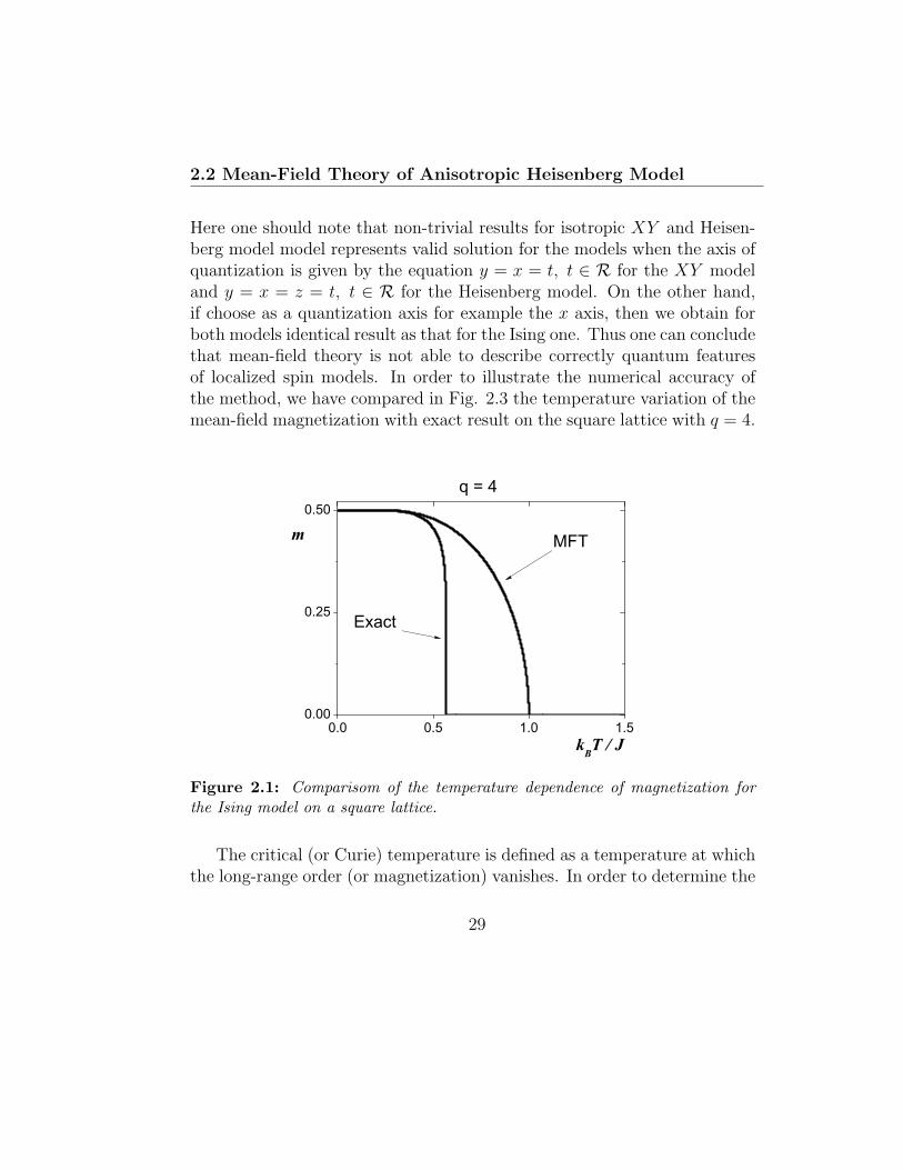
22 Mean-Field Theory of Anisotropic Heisenberg Model
Here one should note that non-trivial results for isotropic XY and Heisen-berg model model represents valid solution for the models when the axis ofquantization is given by the equation y = x = t t isin R for the XY modeland y = x = z = t t isin R for the Heisenberg model On the other handif choose as a quantization axis for example the x axis then we obtain forboth models identical result as that for the Ising one Thus one can concludethat mean-field theory is not able to describe correctly quantum featuresof localized spin models In order to illustrate the numerical accuracy ofthe method we have compared in Fig 23 the temperature variation of themean-field magnetization with exact result on the square lattice with q = 4
00 05 10 15000
025
050q = 4
m
kBT J
Exact
MFT
Figure 21 Comparisom of the temperature dependence of magnetization forthe Ising model on a square lattice
The critical (or Curie) temperature is defined as a temperature at whichthe long-range order (or magnetization) vanishes In order to determine the
29
22 Mean-Field Theory of Anisotropic Heisenberg Model
Curie temperature we take into account that tanh(x) asymp x for x ltlt 1 andobtain an universal solution
Tc =qJα
4kB α = x y z (245)
which valid for all three cases mentioned above Of course the critical tem-perature should be different depending on the model considered Thus thepresent method is not able to distinguish specific features of the models aslong as concerns the critical behavior Moreover it is also clear that thetopology of the lattice is taken into account only through its coordinationnumber that is also weak point of the present method It is well knownthat this approach significantly fails for the low-dimensional systems nev-ertheless it gives rather good qualitative picture for the three-dimensionalsystems and therefore it is frequently used to obtain analytical results par-ticularly for complex systems
Finally one should note that calculations of other thermodynamic quan-tities is easy and straightforward since we have analytical solution for theGibbs free energy of the system from which other quantities are easily ob-tained
This calculation including numerical analysis and discussion is left forthe readers as an appropriate exercise
Let us conclude this part by noticing that the present approach can beextended to case of the the so-called Oguchi approximation which alreadyaccount much better for the quantum effects as well as for the spin-spincorrelations Possible extensions are rather involved and require lengthycalculations that are beyond the scope of the present book
30
Chapter 3
Spin-Wave Theory
31 Bloch Spin-Wave Theory of Ferromag-
nets
In this part we will discuss the concept of spin waves which enables to studythe some physical properties of magnetic systems at low temperatures Thistheory was originally introduced by F Bloch [1] and its main assumptionis that the ground state of the system is ordered and the excited states aredescribed as a collection of spin waves At low temperatures it is reasonableto expect the small amplitudes of the spin waves thus the interaction amongspin waves can be neglected We will consider in this part an isotropicHeisenberg model defined by the Hamiltonian
H = minusJsumij
SiSj minus gmicroBHsumi
Szi (31)
Here Si represents a vector spin-operator at the ith site of the lattice Thisoperator is naturally defined as Si = (Sx
i Syi S
zi ) where Sα
i (α = x y z)represent spatial components of the standard spin operators g is the Lande
31
31 Bloch Spin-Wave Theory of Ferromagnets
factor microB is the Bohr magneton and H denotes the external magnetic fieldwhich is applied along z axis J is the exchange integral which is assumedto be positive since we are going to investigate the ferromagnetic systems
Adopting the basic concept of lattice vibrations we can write the fol-lowing equation of motion of the spin Sℓ on the j th lattice point
dSℓ
dt=
i
~[H Sℓ] (32)
In what follows we will use the following commutation relations for spinoperators
[Sai S
bj ] = iεabcδijS
cj a b c = x y or z (33)
where εabc represents Levi-Civita tensor and δij is the Kronecker symbolNow substituting the Hamiltonian (31) into (32) and employing relations(33) one obtains
dSℓ
dt= minus1
~(Hℓ times Sℓ) (34)
where the local magnetic field Hℓ acting on the j th spin is given by
Hℓ =sumj
JjℓSj + gmicroBHe3 (35)
with e3 = (0 0 1) Using two previous equations one easily obtains thefollowing equations of motion of the x y and z components of the spinoperator
~dSx
ℓ
dt= minus
sumj
Jjℓ(Syj S
zℓ minus Sz
j Syℓ ) + gmicroBHSy
ℓ (36)
~dSy
ℓ
dt= minus
sumj
Jjℓ(Szj S
xℓ minus Sx
j Szℓ )minus gmicroBHSx
ℓ (37)
32
31 Bloch Spin-Wave Theory of Ferromagnets
~dSz
ℓ
dt= minus
sumj
Jjℓ(Sxj S
yℓ minus Sy
j Sxℓ ) (38)
If we restrict ourselves to the case of low-energy excitation then the compo-nents Sx
ℓ Syℓ can be regarded as small quantities of first order Consequently
the right-hand side of (38) is a small quantity of the second order whichcan be neglected and it follows from Eq (38) that the zth component be-comes a constant Moreover it is reasonable to put explicitly Sz
ℓ = S sincethe external magnetic field is assumed to be applied parallel to the zth axisUnder these assumptions Eqs (36) and (37) can be rewritten in the form
~dSx
ℓ
dt= minusS
sumj
Jjℓ(Syj minus Sy
ℓ ) + gmicroBHSyℓ (39)
~dSy
ℓ
dt= minusS
sumj
Jjℓ(Sxℓ minus Sx
j )minus gmicroBHSxℓ (310)
or alternatively
~dS+
ℓ
dt= minusiS
sumj
Jjℓ(S+ℓ minus S+
j )minus gmicroBHS+ℓ (311)
~dSminus
ℓ
dt= minusiS
sumj
Jjℓ(Sminusℓ minus Sminus
j )minus gmicroBHSminusℓ (312)
where we have introduced the spin-raising and spin-lowering operators
S+ℓ = Sx
ℓ + iSyℓ Sminus
ℓ = Sxℓ minus iSy
ℓ (313)
that obey the following commutation rules
[Szk S
+ℓ ] = S+
k δkℓ [Szk S
minusℓ ] = minusSminus
k δkℓ [S+k S
+ℓ ] = 2Sz
kδkℓ (314)
33
31 Bloch Spin-Wave Theory of Ferromagnets
The above relations are directly obtained with the help of well-known com-mutation relations of the spin operators (33)
To proceed further we now express the spin-raising and spin-loweringoperators with the help of the Fourier transform ie
S+q =
1radicN
sumj
eiqmiddotRj S+j Sminus
q =1radicN
sumj
eminusiqmiddotRj Sminusj (315)
S+j =
1radicN
sumq
eminusiqmiddotRj Sq Sminusj =
1radicN
sumq
eiqmiddotRj Sq (316)
Substituting Eq(316) into Eq(312) and applying the following relationsumℓ
eminusi(q1minusq2)middotRℓ = Nδq1q2 (317)
one gets equation
minusi~dSminus
q
dt=
[Ssumℓ
Jjℓ(1minus eminusiqmiddot(RjminusRℓ)) + gmicroBH]Sminusq (318)
If we now introduce a real quantity
J(q) =sumj
J(Rj)eminusiqmiddotRj (319)
then we rewrite (318) as
minusi~dSminus
q
dt=
S[J(0)minus J(q)
]+ gmicroBH
Sminusq (320)
It is straightforward to obtain the solution of this equation in the form
Sq = δSqei(ωqt+α) (321)
34
31 Bloch Spin-Wave Theory of Ferromagnets
where the eigenfrequencies of the spin waves are given by
~ωq = S[J(0)minus J(q)
]+ gmicroBH (322)
One should notice here that in the limit of small q we obtain ~ωq asymp q2Now using Eq(321) we can express the spin operators in the real space
as follows
Sminusj =
1radicNδSqe
i(qmiddotRj+ωqt+α) (323)
Sxj =
1radicNδSq cos
[i(q middotRj + ωqt+ α)
](324)
and
Syj = minus 1radic
NδSq sin
[i(q middotRj + ωqt+ α)
] (325)
Finally it is straightforward to prove that the energy difference betweenan excited state and ground state is given by
Eq minus E0 = ~ωq (326)
where ~ωq represents the excitation energy of the spin wave with the wavevec-tor q The proof of the last statement is left as an appropriate exercise forreaders
35
32 Holstein-Primakoff theory of ferromagnets
32 Holstein-Primakoff theory of ferromag-
nets
The Blochrsquos spin-wave theory discussed in previous chapter represents a verysimple approach in which we completely neglect the interaction among spinwaves This deficiency can be eliminated using an alternative formulationbased on magnon variables (or creation-annihilation operators) developedby Holstein and Primakoff [2] In this part we apply The Holstein-Primakofftheory to case of an anisotropic quantum Heisenberg model described bythe Hamiltonian
H = minusJsumij
(Sxi S
xj + Sy
i Syj + Sz
i Szj )minus gmicroBH
sumi
Szi (327)
The meaning of all symbols in previous Eq (327) is the same as in previoustext
In order to apply a spin-wave picture to analyze magnetic properties ofthe model under investigation one has to perform three subsequent math-ematical transformation At first we express the components of the spinoperators trough spin-lowering and spin raising operators then we intro-duce so-called creation and annihilation operators and finally we performa Fourier transform of the relevant all creation and annihilation operatorsentering the Hamiltonian The eigenvalues of the final Hamiltonian then en-able to determine relevant physical quantities applying standard relationsof statistical mechanics For further manipulations it is more convenient torewrite (327) as follows
H = minusJsumℓδ
(Sxℓ S
xℓ+δ + Sy
ℓ Syℓ+δ + Sz
ℓ Szℓ+δ)minus gmicroBH
sumℓ
Szℓ (328)
where ℓ labels the lattice sites and δ denotes nearest neighbors of the relevantsite and we assume that J gt 0 The integrals of motion for Hamiltonian
36
32 Holstein-Primakoff theory of ferromagnets
(328) are the total z th component Sz =sum
k Szk and the total spin of the
systemThe ground state of the system is ordered and for H gt 0 the magnetic
moment is paralell to the z axis If we consider the lattice consisting of Natoms with spin S then the ground-state vector in the spin basis reads |0⟩= |NSNS⟩ Of course we work in a real space basis in which the spinoperators Sz
ℓ are diagonal We recall that the eigenvalues MS = minusS minusS +1 S and eigenvectors |MS⟩ℓ of the operator Sz
ℓ satisfy the followingequation
Szℓ |MS⟩ℓ = MS|MS⟩ℓ (329)
Now applying operators (313) to the eigenvectors |MS⟩ℓ one obtains
S+ℓ |MS⟩ℓ =
radic(S minusMS)(S minusMS minus 1)|MS + 1⟩ℓ (330)
and
Sminusℓ |MS⟩ℓ =
radic(S +MS)(S minusMS minus 1)|MS minus 1⟩ℓ (331)
In addition to the spin-raising and spin-lowering operators we will alsouse in our analysis the operator describing a deviation of the zth spin-component from its maximum value namely
nℓ = S minus Szℓ (332)
The eigenvalues of this operator are integers nl = 0 1 2 2S (or nl =S minusMS) thus we can rewrite Eqs(330) in the form
S+ℓ |nℓ⟩ℓ =
radic2S
radic1minus (nℓ minus 1)
2S
radicnℓ|nℓ minus 1⟩ℓ (333)
Le us note that performing a similar procedure is also possible for Eq(331)and it will be used later
37
32 Holstein-Primakoff theory of ferromagnets
Now with the help of (313) we can rewrite the Hamiltonian (328) inthe form
H = minusJsumℓδ
[12(S+
ℓ Sminusℓ+δ + Sminus
ℓ S+ℓ+δ) + Sz
ℓ Szℓ+δ
]minus gmicroBH
sumℓ
Szℓ (334)
which is suitable for introducing the Holstein-Primakoff magnon represen-tation In order to define the relevant transformation we at first introducethe standard creation and annihilation operators that are defined as
adaggerℓΨnℓ=
radicnℓ + 1Ψnℓ+1 aℓΨnℓ
=radicnℓΨnℓminus1 (335)
The central idea of the Holstein-Primakoff approach is based on the intro-duction of the following transformation
S+ℓ = (2S)12
(1minus adaggerℓaℓ
2S
)12
aℓ (336)
Sminusℓ = (2S)12adaggerℓ
(1minus adaggerℓaℓ
2S
)12
(337)
Szℓ = S minus adaggerℓaℓ (338)
As already noted above the eigenvalues of adaggerℓaℓ are arbitrary integers whilethat of nℓ are limited to the range 0 le nℓ le 2S Fortunately this discrep-ancy does not play any important role in the calculation since the transitionfrom the state with nℓ le 2S to states with nℓ gt 2S never occur eg
Sminusℓ Ψ2S = (2S)12(2S + 1)12
(1minus 2S
2S
)12
Ψ2S+1 = 0 (339)
Now we transform the operators aℓ adaggerℓ from the real space to the reciprocal
space by the following Fourier tansform
aℓ =1radicN
sumq
eminusiqmiddotRℓbq (340)
38
32 Holstein-Primakoff theory of ferromagnets
adaggerℓ =1radicN
sumq
eiqmiddotRℓbdaggerq (341)
where N denotes the total number of atoms q represents a vector of thereciprocal space and Rℓ represents a vector specifying the position of ℓthatom in the lattice
The magnon-annihilation and magnon-creation operators are given by
bq =1radicN
sumℓ
eiqmiddotRℓaℓ (342)
bdaggerq =1radicN
sumℓ
eminusiqmiddotRℓadaggerℓ (343)
and they obey the usual magnon commutation relations
[bq1 bdaggerq2] = δq1q2 [bq1 bq2 ] = [bdaggerq1
bdaggerq2] = 0 (344)
It is useful to note here that the operator bdaggerq creates a magnon with thewave vector q and the operator bq annihilates it Moreover it follows fromthe transformation (340) and (341) that any change of the spin state atarbitrary lattice site is described as a superposition of an infinite number ofthe spin waves
At this stage it is clear that further exact treatment of the problem isimpossible due to the complexity of applied transformations The progressis however still possible if we restrict ourselves to the case when the numberof excited states is small in comparison with 2S Under this assumptionwe can neglect the higher order terms in expansion of the square root andrewrite Eqs (336) and (337) in the form
S+ℓ = (2S)12
(1minus adaggerℓaℓ
4S
)aℓ + (345)
39
32 Holstein-Primakoff theory of ferromagnets
Sminusℓ = (2S)12adaggerℓ
(1minus adaggerℓaℓ
4S
)+ (346)
Finally substituting (340) and (341) into previous equation one obtains
S+ℓ =
(2S
N
)12[sumq1
eminusiq1middotRℓbq1 minus1
4SN
sumq1q2q3
ei(q1minusq2minusq3)middotRℓbdaggerq1bq2bq3 +
](347)
Sminusℓ =
(2S
N
)12[sumq1
eiq1middotRℓbdaggerq1minus 1
4SN
sumq1q2q3
ei(q1+q2minusq3)middotRℓbdaggerq1bdaggerq2
bq3 +
](348)
Similarly the operator Szℓ is given by
Szℓ = S minus 1
N
sumq1q2
ei(q1minusq2)middotRℓbdaggerq1bq2 (349)
If we assume that each lattice site has z nearest neighbors then we canspecify their positions on the lattice by introducing the vector
δ = Rℓ+δ minusRℓ (350)
Substituting (347)-(350) into Eq(334) and performing a rearrange-ment of the terms one can rewrite the Hamiltonian as
H = minusJNzS2 minus gmicroBNHS + H0 + H1 (351)
where H0 is a bilinear form in the magnon variables and it is given by
H0 = minus JS
N
sumℓδ
sumq1q2
[eminusi(q1minusq2)middotRℓeiq2middotδbq1b
daggerq2
+ ei(q1minusq2)middotRℓeminusiq2middotδbdaggerq1bq2
]+
JS
N
sumℓδ
sumq1q2
[ei(q1minusq2)middotRℓbq1b
daggerq2
+ eminusi(q1minusq2)middotRℓei(q1minusq2)middotδbdaggerq1bq2
]+
gmicroBH
N
sumℓq1q2
ei(q1minusq2)middotRℓbdaggerq1bq2 (352)
40
32 Holstein-Primakoff theory of ferromagnets
The term H1 includes higher-order terms and for the sake of simplicity willbe neglected Now taking into account the relation (317) and performingthe summation over ℓ and q2 we can simplify Eq(352) as follows
H0 = minusJzSsumq
(γqbqbdaggerq + γminusqb
daggerqbq minus 2bdaggerqbq) + gmicroBH
sumq
bdaggerqbq (353)
where
γq =1
z
sumδ
eiqmiddotδ (354)
and the summation in (354) runs over all nearest neighbors For furthermanipulation it useful noticing that
sumq γq = 0 and moreover for the crys-
tals with the symmetry center we have γq = γminusk Employing the magnoncommutation rules [bdaggerqbq] = 1 one obtains
H0 =sumq
[2JzS(1minus γq) + gmicroBH
]bdaggerqbq (355)
The last equation can be rewritten in the following very simple form
H0 =sumq
~ωqnq (356)
where nq is the magnon occupation operator and
~ωq = 2JzS(1minus γq) + gmicroBH (357)
Since the quantity γq can be expressed as follows
γq =1
z
sumδ
eiqmiddotδ =1
2z
sumδ
(eiqmiddotδ + eminusiqmiddotδ) =1
2z
sumδ
cos(q middot δ) (358)
then the dispersion relation becomes
~ωq = 2JzS[1minus 1
2z
sumδ
cos(q middot δ)]+ gmicroBH (359)
41
32 Holstein-Primakoff theory of ferromagnets
321 Internal Energy and Specific heat
In this subsection we will show how one can calculate the internal energyand specific heat of Heisenberg model within the Holstein-Primakoff theoryBefore performing any calculation it is useful noticing that due to neglectinghigher order terms in Eq (345) and (346) we treat the ensemble of non-interacting magnons In further calculatiuon we also will assume H = 0and |q middot δ| ≪ 1
Under these assumptions the internal energy of the magnon gas in ther-modynamic equilibrium at temperature T can be expressed as
U =sumq
~ωq⟨nq⟩ (360)
where ⟨nq⟩ is given by the well-known Bose-Einstein relation
⟨nq⟩ =[exp
( ~ωq
kBT
)minus 1
]minus1
(361)
Substituting (361) into (360) one gets
U =sumq
~ωq
[exp
( ~ωq
kBT
)minus 1
]minus1
=1
(2π)3
intDq2
[exp
(Dq2
kBT
)minus 1
]minus1
d3q
=1
2π2
intDq4
[exp
(Dq2
kBT
)minus 1
]minus1
dq (362)
where we have introduced the lattice stiffnes as D = 2SJa2 If we denotex = Dq2kBT then we can rewrite (362) as
U =(kBT )
52
4π2D32
int xm
0
x32
exp(x)minus 1dx (363)
42
32 Holstein-Primakoff theory of ferromagnets
The last expression can be further simplified by considering the regionkBT ≪ ωmax Then the upper limit in the integral (363) can be approxi-mated by infinity and one obtains for internal energy the following analyticalexpression for internal energy of the system
U =(kBT )
52
4π2D32Γ(52
)ζ(52 1) (364)
Here Γ and ζ denote the Gamma- and Riemann zeta-functions respectively
and their numerical values of relevant arguments are known to be Γ(
52
)=
3radicπ
4and ζ
(52 1)= 1341
Thus we finally obtain
U ≃ 045(kBT )52
π2D32 (365)
Consequently for the magnetic part of specific heat at constant volume isgiven by
CV = 0113kB
(kBTD
) 32 (366)
In this work we consider strictly insulating materials thus there is no elec-tron contribution to the total specific heat Consequently taking into ac-count the phonon and magnon contribution we can express the total specificheat at low temperatures by the formula
C = aT 3 + bT 32 (367)
It is clear from this equation that the magnon contribution can experimen-tally easily determined if we plot the dependence of reduced specific heatCT 32 versus T 32 The situation is schematically illustrated in Fig 31
43
32 Holstein-Primakoff theory of ferromagnets
0 2 4 6 80
1
2
CT -32
T 32
magnoncontribution
Figure 31 The re-scaled specific heat vs T 32
322 Magnetization and Critical Temperature
The magnetic moment of the system can be calculated from the equation
MS = gmicroB
⟨(NS minus
sumq
bdaggerqbq)⟩ (368)
The deviation of the magnetization from its saturation value can be ex-pressed as
∆M = M(0)minusM(T ) = gmicroB
sumq
⟨nq⟩
=gmicroB
(2π)3
int qm
0
[exp
(Dq2
kBT
)minus 1
]minus1
d3q (369)
44
33 Holstein-Primakoff theory of antiferromagnets
At low temperatures (Dq2 ≫ kBTJ) we obtain
∆M =gmicroB
2π2
(kBTJD
)32int infin
0
x12
exp(x)minus 1dx
=gmicroB
2π2
(kBTJD
)32
Γ(52
)ζ(32 1)
= 0117gmicroB
(kBTD
)32
(370)
The finite-temperature magnetization can be then expressed as
M(T ) = M(0)[1minus
( T
Tc
) 32]
(371)
where the critical temperature Tc is given by
Tc =( M(0)
0117gmicroB
) 23 D
kB (372)
33 Holstein-Primakoff theory of antiferro-
magnets
The Holstein-Primakoff theory can be extended also to the case of antifero-magnetic Heisenberg model which can describe many real materials [7] Onthe other hand the generalization of the Holstein-Primakoff for quantumantiferromagnets is very interesting because such systems exhibit very inter-esting magnetic properties that differ from quantum ferromagnets in manyrespects Our aim in this subsection is to investigate the antiferromagneticHeisenberg model spin system consisting of two interpenetrating sublatticesa and b which is described by the Hamiltonian
H = minusJsumij
SaiSbj minus gmicroBHa
sumi
Szai + gmicroBHa
sumj
Szbj (373)
45
33 Holstein-Primakoff theory of antiferromagnets
where J lt 0 is the exchange interaction which couples the nearest neighborson lattice and the quantity Ha gt 0 represents an external magnetic fieldwhich is parallel to the z axis In what follows we will treat the problem ap-plying the Holstein-Primakoff transformation for each sublattice separatelyAt first we express the spin rising and lowering sublattice operators withthe help of creation-annihilation operators as follows
S+aj = (2S)12
(1minus
adaggerjaj
2S
)12
aj Sminusaj = (2S)12adaggerj
(1minus
adaggerjaj
2S
)12
(374)
S+bℓ = (2S)12
(1minus bdaggerℓbℓ
2S
)12
bℓ Sminusbℓ = (2S)12bdaggerℓ
(1minus bdaggerℓbℓ
2S
)12
(375)
Szaj = S minus adaggerjaj minusSz
bℓ = S minus bdaggerℓbℓ (376)
Next we introduce the sublattice spin-wave variables
cq =2radicN
sumj
eminusiqmiddotRjaj cdaggerq =2radicN
sumj
eiqmiddotRjadaggerj (377)
dq =2radicN
sumℓ
eiqmiddotRℓbℓ ddaggerq =2radicN
sumℓ
eminusiqmiddotRℓbdaggerℓ (378)
In previous equations summations run over all N atoms of the a and b sub-lattice respectively Moreover the following magnon commutation relationshold
[cq1 cdaggerq2] = [dq1 d
daggerq2] = δq1q2
[cq1 cq2 ] = [cdaggerq1 cdaggerq2
] = 0 [dq1 dq2 ] = [ddaggerq1 ddaggerq2
] = 0 (379)
46
33 Holstein-Primakoff theory of antiferromagnets
Now we expand (374)-(375) as
S+aj =
(4S
N
)12[sumq1
eminusiq1middotRjcq1 minus1
8SN
sumq1q2q3
ei(q1minusq2minusq3)middotRjcdaggerq1cq2cq3 +
](380)
Sminusaj =
(4S
N
)12[sumq1
eiq1middotRjcdaggerq1minus 1
8SN
sumq1q2q3
ei(q1+q2minusq3)middotRjcdaggerq1cdaggerq2
cq3 +
](381)
S+bℓ =
(4S
N
)12[sumq1
eminusiq1middotRℓdq1 minus1
8SN
sumq1q2q3
ei(q1minusq2minusq3)middotRℓddaggerq1dq2dq3 +
](382)
Sminusbℓ =
(4S
N
)12[sumq1
eiq1middotRℓddaggerq1minus 1
8SN
sumq1q2q3
ei(q1+q2minusq3)middotRℓddaggerq1ddaggerq2
dq3 +
](383)
Szaj = S minus 1
N
sumq1q2
ei(q1minusq2)Rjcdaggerq1cq2 (384)
Szbℓ = minusS +
1
N
sumq1q2
eminusi(q1minusq2)Rℓddaggerq1dq2 (385)
Substituting these expansions into (373) and using (317) we obtain
H = NzJS2 + H0 + H1 (386)
47
33 Holstein-Primakoff theory of antiferromagnets
where H0 is a part of the Hamiltonian which is bilinear in magnon variablesie
H0 = minus2JzSsumq
[γq(cdaggerqd
daggerq + cqdq
)+(cdaggerqcq + ddaggerqdq
)]+ gmicroBH
sumq
(cdaggerqcq minus ddaggerqdq
)(387)
where γq is given by (354) and the existence of symmetry center of the
lattice has been assumed The quantity H1 includes higher-order termsand will be for the simplicity neglected However even after neglectingH1 the energy spectrum of system cannot be simply obtained since theHamiltonian is not yet diagonal Thus the main problem to be solved is thediagonalization of H0 In order to make a progress we introduce here newset of the creation and annihilation operators αdagger
q αq βdaggerq βq
αq = uqcq minus vqddaggerq αdagger
q = uqcdaggerq minus vqdq (388)
βq = uqdq minus vqcdaggerq βdagger
q = uqddaggerq minus vqcq (389)
obeying the following commutation rules
[αq αdaggerq] = 1 [βk β
daggerq] = 1 [αq βq] = 0 (390)
The real quantities entering previous equations satisfy relation
u2q minus v2q = 1 (391)
and the inverse transformation are given by
cq = uqαq minus vqβdaggerq cdaggerq = uqα
daggerq minus vqβq (392)
dq = uqβq minus vqαdaggerq ddaggerq = uqβ
daggerq minus vqαq (393)
48
33 Holstein-Primakoff theory of antiferromagnets
The parameters uq and vq in transformations (392) and (393) can be de-termined explicitly in the form
uq = cosh θq vq = sinh θq (394)
where θq is given by
tanh(2θq) = γq (395)
The explicit forms of the transformation given by (394) and (395) is usuallycalled in the literature as Bogolyubov transformation Substituting (392)and (393) into (387) one finally obtains for H the folloving simple relation
H = NJzS(S + 1) +sumq
[~ω+
q
(αdaggerqαq +
1
2
)+ ~ωminus
q
(βdaggerqβq +
1
2
)](396)
where we have defined the eigenfrequencies of the system as
~ωplusmnq = minus2JzS
radic1minus γ2
q plusmn gmicroBH (397)
331 Ground-State Energy
In this part we investigate the ground-state energy of the two sublatticeantiferromagnetic Heisenberg system
The lowest possible energy (ie the ground-state energy) can be straight-forwardly obtained after setting H = 0 and averaging Eq(396)
Eg equiv ⟨H⟩ = NJzS(S + 1) +sumq
[~ω+
q
(⟨αdagger
qαq⟩+1
2
)+ ~ωminus
q
(⟨βdagger
qβq⟩+1
2
)]
(398)
Of course the ground state corresponds to the vacuum state in which no ex-cited magnons are present in the system and therefore the previous equation
49
33 Holstein-Primakoff theory of antiferromagnets
reduces to
Eg = NJzS(S + 1)minus 2JzSsumq
(1minus γ2
q
)12
= NJzS2[1 +
1
S
(1minus 2
N
sumq
radic1minus γ2
q
)] (399)
The parameter γq depends on the lattice structure and it is given by
γq =1
d
dsumi=1
cos qi (3100)
where d = 1 for the one-dimensional chain d = 2 for two-dimensionalsquare and d = 3 for three-dimensional simple-cubic lattice respectivelyIn order to find numerical values of Eg we have to evaluate the sum over qin Eq (399) which must be taken over all N2 points in the first Brillouinzone of the sublattice The relevant sum can be expressed as
Id =2
N
radic1minus γ2
q
=1
(2π)d
int π
minusπ
int π
minusπ
dq1 dqd
[1minus
(1d
dsumi=1
cos qi
)2]12 (3101)
Evaluating the above expression one gets
I1= 0637 I2
= 0842 I3
= 0903 (3102)
and using these numerical values we obtain the ground-state energy in the
50
33 Holstein-Primakoff theory of antiferromagnets
form
Eg = 2NJS2(1 +
0363
S
)for the linear chain
Eg = 4NJS2(1 +
0158
S
)for the square lattice (3103)
Eg = 6NJS2(1 +
0097
S
)for the cubic lattice
One should note here that all numerical values of the ground-state energysatisfy the Anderson inequality
1
2NJzS2(1 +
1
zS) lt Eg lt
1
2NJzS2 (3104)
It is also useful to note that for the spin-12 linear chain Eq(3104) givesthe value Eg(NJ) = 0863 which is in agreement with the exact Bethe-Hulten [3 4] value Eg(NJ) = 05(4 ln 2 minus 1) = 0886 On tha basis ofthis excellent agreement one should assume that the spin-wave theory givesacceptable quantitative results also for other lattices and spin values
The most important qualitative finding in this part is the fact that theenergy corresponding to the saturated antiparallel ordering is not the groundstate energy of the two-sublattice antiferromagnetic system This finding isa direct consequence of the fact that the total sublattice magnetization arenot the constants of motion
332 Sublattice Magnetization
At first let us examine in this part the ground-state sublattice magnetizationwhich is defined as
Ma = gmicroB
⟨sumj
Szaj
⟩=
1
2NS minus
sumq
⟨cdaggerqcq
⟩(3105)
51
33 Holstein-Primakoff theory of antiferromagnets
Using the Bogolyubov transformation (394) we obtain
Ma =1
2NS minus
sumq
cosh2(θq)
⟨αdaggerqαq
⟩+sinh2(θq)
⟨βqβ
daggerq
⟩minus sinh(θq) cosh(θq)(
⟨αdaggerqβ
daggerq
⟩+⟨αqβq
⟩)
(3106)
At zero temperature there are no excited states and therefore Eq(3106)simplifies as follows
Ma =1
2NS minus
sumq
sinh2(θq) (3107)
After substituting the relevant expression for sinh(θq) one obtains expression
Ma =1
2NS minus 1
4
sumq
[(1minus γq1 + γq
)12
+
(1 + γq1minus γq
)12
minus 2
] (3108)
which can finally be rewritten as
Ma =NS
2
[1minus 1
2S
(2
N
sumq
1radic1minus γ2
q
minus 1
)] (3109)
In order to proceed further we express the sum Sd =2N
sumq
1radic1minusγ2
q
appearing
in (3109) in the following integral form
Sd =2
N
sumq
1radic1minus γ2
q
=1
(2π)d
int π
minusπ
middot middot middotint π
minusπ
dλ1 dλd
[1minus
(1
d
dsumj=1
cosλj
)2]minus12
(3110)
52
33 Holstein-Primakoff theory of antiferromagnets
Evaluating this integral for the simple cubic lattice (d = 3) and plane squarelattice (d = 2) one obtains values S3 = 1156 and S2 = 1393 from whichthe sublattice magnetization are given by
Ma =NS
2
(1minus 0078
S
)for d = 3 (3111)
Ma =NS
2
(1minus 0197
S
)for d = 2 (3112)
Thus we can conclude that the spin-wave theory predicts a long-range or-der in three- and two dimensional antiferromagnetic Heisenberg systemshowever as it is clear from (3110)-(3112) the sublattice magnetizationsdo not take their saturation values at zero temperature This behavior ap-pears due to quantum fluctuations at the ground state that are stronger inlower dimensions
In the case of linear chain (d = 1) the integral S1 diverges logarith-mically indicating that the sublattice magnetization has zero expectationvalue This result is in agreement with exact calculations and represents asignificant improvement over the standard mean-field theory which predictsthe existence of long-range order also for one dimensional Heisenberg model
Finally let us comment on the calculation of the temperature depen-dence of the sublattice magnetization for the antiferromagnetic Heisenbergmodel The deviation of the sublattice magnetization from its ground-statevalue is calculated from
Ma(0)minusMa(T ) =sumq
⟨nq⟩ cosh(2θq)
=sumq
⟨nq⟩(1minus γ2
q
)minus12(3113)
where the mean number of bosons is obviously given by
⟨nq⟩ =1
exp( ~ωq
kBT
)minus 1
(3114)
53
33 Holstein-Primakoff theory of antiferromagnets
with
~ωq = (2JSz)2(1minus γ2q) (3115)
However the explicit calculation of sublattice magnetizations at arbitrarytemperature represents hard and non-trivial mathematical task Neverthe-less at the temperatures that are significantly lower then the Neel transitiontemperature TN one finds that the sublattice magnetization is proportionalto (TTN)
2 The proof of this behavior is left for the reader
54
Chapter 4
Jordan-Wigner Transformationfor the XY Model
In previous parts of this text we have discussed how to apply the bosoniza-tion technique within the Holstein-Primakoff approach to the ferromagneticand antiferromagnetic spin systems In the present chapter we will investi-gate a similar approach which is known as a method of fermioniozation Inparticular we will discuss application of the Wigner-Jordan transformationto the isotropic quantum XY model in order to clarify important points ofthis method
The main idea of this approach is to transform the Hamiltonian de-scribing a spin system by the use of new operators obeying the fermionanticommutation rules
Before we start our analysis it is useful to note that the spectrum of theXY model was exactly found by HBethe [3] in 1931 The Bethersquos approachis of great importance however it is quite involved and rather abstractthus it is difficult to understand even such basic properties as long-rangeorder A much more natural approach to the problem of interacting spin-12 systems was originally introduced in 1928 by Jordan and Wigner [5]
55
41 Jordan-Wigner Transformation for the XY Model
who invented simple mathematical transformations converting spin-12 sys-tems into problems of interacting (and in some cases even non-interacting)spinless fermions In fact the XY model which is a special case of theHeisenberg Hamiltonian reduces to a free theory of spinless fermions un-der the Jordan-Wigner transformations Another reason for choosing theXY model is that the low-energy properties of the full anti-ferromagneticHeisenberg chain such as the presence of gapless excitations and absenceof a long range order are very similar to those of the XY model (see [6] andreferences therein)
We will study a linear chain of N spin-12 atoms interacting antiferro-magnetically with their nearest neighbors This system is described by theHamiltonian
H = JNsumj=1
(Sxj S
xj+1 + Sy
j Syj+1) (41)
where J gt 0 represents the exchange interaction ans Sαi are spin-12 opera-
tors obeying the usual commutation relations (33) As usually we assumecyclic boundary conditions with Sα
N+1 = Sα1 α = x y Of course for
J lt 0 the ferromagnetic case of (41) is obtained Thus if we solve theantiferromagnetic problem exactly then we can immediately obtain alsothe solution of the ferromagnetic XY chain Similarly as in the case ofbozonization we at first introduce spin-raising and spin-lowering operators(313) and rewrite the Hamiltonian as a bilinear form in these operatorsie
H =J
2
Nsumj=1
(Sminusj S
+j+1 + Sminus
j+1S+j ) (42)
It clear that without loss of generality we can set J = 1 in all subsequentcalculations We know that the Splusmn operators belonging to the same siteobey anticommutation relations while that ones on different sites satisfy
56
41 Jordan-Wigner Transformation for the XY Model
usual commutation relations and this mathematical property disables a di-rect diagonalization of (42) The key to the solution of this problem is theJordan-Wigner transformation which enables to obtain the Hamiltonian interms of pure fermion operators
The JordanndashWigner transformation explicitly reads
cdaggern = S+n exp
(minusiπ
nminus1sumj=1
S+j S
minusj
) cn = Sminus
n exp(iπ
nminus1sumj=1
S+j S
minusj
) (43)
and the inverse transformation is given by
S+n = cdaggern exp
(iπ
nminus1sumj=1
cdaggerjcj
) Sminus
n = cn exp(iπ
nminus1sumj=1
cdaggerncn
) (44)
Here it is worth noticing that the signs in the exponents and the order ofthe multipliers in (43) and (44) are not important
The operators cdaggerj ck obey the canonical fermion algebra ie
cj cdaggerk = δjk cdaggerj cdaggerk = 0 cj ck = 0 (45)
To illustrate the mathematics behind we will explicitly prove the first rela-tion while the other anti-commutators in (45) can be computed in a similarfashion
At first we recall the validity of the following relations [S+j Sj S
+k Sk] = 0
[S+j Sj Sk] = minusδjkSk [S
+j Sj S
+k ] = δjkS
+k (S
+j Sj)
2 = S+j Sj since the spin-
raising and spin-lowering operators on different sites commute and on thesame site behave like fermions Therefore
exp(plusmniπ
msumj=n
S+j S
minusj
)=
mprodj=n
exp(plusmniπS+j S
minusj ) (46)
57
41 Jordan-Wigner Transformation for the XY Model
and the exponential function on the rhs of previous equation can be easilyevaluated as follows
exp(plusmniπS+j S
minusj ) =
infinsumk=0
1
k(plusmniπ)k(S+
j Sminusj )
k
= 1 +infinsumk=1
1
k(plusmniπ)kS+
j Sminusj
= 1 + (eplusmniπ minus 1)S+j S
minusj = 1minus 2S+
j Sminusj (47)
Similarly using the following anticommutators
Sminusj 1minus 2S+
j Sminusj = 0 S+
j 1minus 2S+j S
minusj = 0 (48)
one obtains relations[exp
(plusmniπ
msumj=n
S+j S
minusj
) Sminus
k
]=
[exp
(plusmniπ
msumj=n
S+j S
minusj
) S+
k
]= 0 k isin [nm]
(49)
exp
(plusmniπ
msumj=n
S+j S
minusj
) Sminus
k
=
exp
(plusmniπ
msumj=n
S+j S
minusj
) S+
k
= 0 k isin [nm]
(410)
Although all the above calculations have a preparatory character they are ofcrucial importance to demonstrate the fermionic nature of cj and cdaggerk Reallyusing (46)- (410) we can now straightforwardly calculate the following
58
41 Jordan-Wigner Transformation for the XY Model
anti-commutators
cj cdaggerk = Sminusj exp
(iπ
jminus1sumℓ=1
S+ℓ S
minusℓ
)exp
(minusiπ
kminus1sumℓ=1
S+ℓ S
minusℓ
)S+k
+ S+k exp
(minusiπ
kminus1sumℓ=1
S+ℓ S
minusℓ
)exp
(iπ
jminus1sumℓ=1
S+ℓ S
minusℓ
)Sminusj
= Sminusj exp
(iπ
kminus1sumℓ=j
S+ℓ S
minusℓ
)S+k S
+k exp
(iπ
kminus1sumℓ=j
S+ℓ S
minusℓ
)Sminusk
= (Sminusj S
+j minus S+
j Sminusj ) exp
(iπ
kminus1sumℓ=j
S+ℓ S
minusℓ
)= 0 k gt j (411)
In the same way we derive relation
cj cdaggerk = ck cdaggerkdagger = 0 k lt j (412)
ck cdaggerk = Sminusk S
+k + S+
k Sminusk = 1 (413)
Thus we have successfully proved the fermionic commutation relations andnow we can transform the relevant terms in the Hamiltonian
For 1 le j le N minus 1 one obtains
Sminusj S
+j+1 = exp
(minusiπ
jminus1sumℓ=1
cdaggerℓcℓ
)cjc
daggerj+1 exp
(iπ
jsumℓ=1
cdaggerℓcℓ
)= cj exp
(minusiπ
jminus1sumℓ=1
cdaggerℓcℓ
)exp
(iπ
jsumℓ=1
cdaggerℓcℓ
)cdaggerj+1
= cj exp(iπcdaggerjcj)c
daggerj+1 = cj(1minus 2cdaggerjcj)c
daggerj+1
= minus(1minus 2cdaggerjcj)cjcdaggerj+1) = minuscjc
daggerj+1 = cdaggerj+1cj (414)
and similarly we have
Sminusj+1S
+j = (Sminus
j S+j+1)
dagger = cdaggerjcj+1 (415)
59
41 Jordan-Wigner Transformation for the XY Model
Here one should notice that in deriving previous equations we have usedthe following relations
[cdaggerjcj cdaggerkck] = 0 (cdaggerjcj)
2 = cdaggerjcj
[cdaggerjcj ck] = minusδjkck [cdaggerjcj cdaggerk] = minusδjkc
daggerk
1minus 2cdaggerjcj cj = 0 1minus 2cdaggerjcj cdaggerj = 0 (416)
[exp
(plusmniπ
msumj=n
cdaggerjcj
) ck
]=
[exp
(plusmniπ
msumj=n
cdaggerjcj
) cdaggerk
]= 0
k isin [nm] (417)
exp
(plusmniπ
msumj=n
cdaggerjcj
) ck
=
exp
(plusmniπ
msumj=n
cdaggerjcj
) cdaggerk
= 0
k isin [nm] (418)
After expressing the special cyclic boundary term (SminusN S
+1 + Sminus
1 S+N) in
terms of crsquos and substituting Eqs(414) and (415) into Eq(42) we canrewrite the Hamiltonian of the system as
H =1
2
sumj
(cdaggerj+1cj + cdaggerjcj+1) + Hb (419)
where
Hb = minus1
2
(cdagger1cN + cdaggerNc1
)[1 + exp
(plusmniπ
Nsumj=1
cdaggerjcj
)](420)
represents the boundary term which gives an O(Nminus1) contributions to themacroscopic physical quantities and for this reason will be neglected infurther calculations
60
41 Jordan-Wigner Transformation for the XY Model
Applying this simplification we are left with the problem of diagonal-ization of the following bilinear form
H =1
2
sumj
(cdaggerj+1cj + cdaggerjcj+1) (421)
which describes free spinless fermions on a cyclic chain with nearest neighborhopping
In order to diagonalize the Hamiltonian (421) we rewrite it in the form
H =sumjk
cdaggerjAjkck (422)
where the elements of the matrix A are given by
Ajk =1
2(δjk+1 + δkj+1) (423)
Taking into account the translational invariance of the lattice we find theeigenvectors and eigenvalues of A to be
ϕqj =1radicNeiqj Λq = cos(q) (424)
with q = 2πnN
and N2 le n le N2 minus 1 The eigenfunctions ϕqk form anorthonormal and complete set thus we can introduce new operators obeyingthe canonical anticommutation rule
ηq =sumj
ϕlowastqjcj ηdaggerq =
sumj
ϕqjcdaggerj (425)
Using the following inverse transformations
cj =sumq
ϕqjηq cdaggerj =sumq
ϕqjηdaggerq (426)
61
41 Jordan-Wigner Transformation for the XY Model
the Hamiltonian (422) can be rewritten in the diagonal form
H =sumq
Λqηdaggerqηq (427)
Since some of the eigenvalues of A will be negative we perform an additionaltransformation
ξq = ηq Λq ge 0 (428)
ξq = ηdaggerq Λq lt 0 (429)
and obtain
H =sum
qΛqge0
Λqξdaggerqξq +
sumqΛqlt0
Λqξdaggerqξq
=sumqΛq
|Λq|ξdaggerqξq minussum
qΛqlt0
|Λq|
=sumqΛq
|Λq|(ξdaggerqξq minus
1
2
) (430)
Here the ξ operators again obey the canonical anticommutation rulesAs usually the ground state |0⟩ satisfies equation
ξq|0⟩ = 0 forallq (431)
and the operator ξdaggerq generates an elementary fermion excitation with energy|Λq| above the ground state
The dispersion relation for the model under investigation is shown in Fig41 As one can see there always exist gapless excitations near q = plusmnπ2The ground state energy reduced per one spin is given by
U0 =⟨H⟩N
= minus 1
N
sumq
1
2|Λq|
=
int π
π
dq
4π| cos(q)| = minus 1
π
int π2
0
cos(q)dq = minus 1
π(432)
62
41 Jordan-Wigner Transformation for the XY Model
ω(q)
0
02
04
06
08
1
q-20 -15 -10 -05 00 05 10 15 20
Figure 41 Dispersion relation of the XY model
Of course the method of fermionization can been extended to manyother systems including the systems with higher spin and higher spatialdimensions However the analysis of this systems requires complex andtedious calculations and sometimes also the applications additional theo-retical tools methods (for example the Green function technique) that arebeyond the scope of this introductory text
63
Conclusion
Conclusion
In this work we have discussed some theoretical tools that are frequentlyused to investigate the localized quantum spin models
The first approach is the standard mean-field theory which representsthe simplest possible technique usually applied to understand basic quan-titative features of various theoretical models of quantum magnetism Al-though this method is included in many textbooks the formulation is usu-ally very simplified and frequently the authors do not derive the Gibbsfree energy within this method To avoid this problem we have used andelegant formulation based on the Bogolyubov inequality which enables toextend our approach to formulate more accurate theories (for example theOguchi approximation or Constant Coupling Method) One should also em-phasize that in deriving the partition function we have applied the Cauchyintegral formula which enables to calculate exponential function with a ma-trix argument This is an unknown trick which can be used in calculationsin nay branch of theoretical physics
In the Chapter 3 we have discussed the standard spin-wave theory sep-arately for ferromagnetic and antiferromagnetic materials We have shownin detail how to introduce the boson operators that enable to calculate sev-eral physical quantities such as magnetization internal energy and magneticcontribution to the specific heat
The last part is dedicated to the method of fermionization Here we havediscussed the application o Jordan-Wigner transformation to the quantumXY model with spin 12 This approach represent another standard theo-retical approach which is used to investigate quantum magnetism
It is clear from the content of this supporting text that we have coveredjust one special part of quantum theory of magnetism which is howeverdiscussed elementary enough In order to understand further interesting fea-tures of the quantum magnetism it is necessary to study further textbooksfor example [8] [9] [10] [11] )
64
Bibliography
[1] F Bloch Z Physik 61 206 (1930)
[2] T Holstein and H Primakoff Phys Rev 58 1908 (1940)
[3] H Bethe Z Physik 71 205 (1931)
[4] L Hulten Ark Met Asron Fysik 26 A 11 (1938)
[5] P Jordan and E Wigner Z Phys 47 631 (1928)
[6] A Tsvelik Quantum Field Theory in Condensed Matter PhysicsCambridge Cambridge University Press 1995
[7] LJ de Jongh AR Miedema Adv Phys 23 2 (1974)
[8] C Kittel Quantum Theory of Solids New York John Wiley andSons 1987
[9] K Yosida Theory of Magnetism Berlin Springer 1998
[10] P Mohn Magnetism in the Solid State Berlin Springer 2003
[11] N Majlis The Quantum Theory of Magnetism Singapore World Sci-entific 2007
65
31 Bloch Spin-Wave Theory of Ferromagnets
where the eigenfrequencies of the spin waves are given by
~ωq = S[J(0)minus J(q)
]+ gmicroBH (322)
One should notice here that in the limit of small q we obtain ~ωq asymp q2Now using Eq(321) we can express the spin operators in the real space
as follows
Sminusj =
1radicNδSqe
i(qmiddotRj+ωqt+α) (323)
Sxj =
1radicNδSq cos
[i(q middotRj + ωqt+ α)
](324)
and
Syj = minus 1radic
NδSq sin
[i(q middotRj + ωqt+ α)
] (325)
Finally it is straightforward to prove that the energy difference betweenan excited state and ground state is given by
Eq minus E0 = ~ωq (326)
where ~ωq represents the excitation energy of the spin wave with the wavevec-tor q The proof of the last statement is left as an appropriate exercise forreaders
35
32 Holstein-Primakoff theory of ferromagnets
32 Holstein-Primakoff theory of ferromag-
nets
The Blochrsquos spin-wave theory discussed in previous chapter represents a verysimple approach in which we completely neglect the interaction among spinwaves This deficiency can be eliminated using an alternative formulationbased on magnon variables (or creation-annihilation operators) developedby Holstein and Primakoff [2] In this part we apply The Holstein-Primakofftheory to case of an anisotropic quantum Heisenberg model described bythe Hamiltonian
H = minusJsumij
(Sxi S
xj + Sy
i Syj + Sz
i Szj )minus gmicroBH
sumi
Szi (327)
The meaning of all symbols in previous Eq (327) is the same as in previoustext
In order to apply a spin-wave picture to analyze magnetic properties ofthe model under investigation one has to perform three subsequent math-ematical transformation At first we express the components of the spinoperators trough spin-lowering and spin raising operators then we intro-duce so-called creation and annihilation operators and finally we performa Fourier transform of the relevant all creation and annihilation operatorsentering the Hamiltonian The eigenvalues of the final Hamiltonian then en-able to determine relevant physical quantities applying standard relationsof statistical mechanics For further manipulations it is more convenient torewrite (327) as follows
H = minusJsumℓδ
(Sxℓ S
xℓ+δ + Sy
ℓ Syℓ+δ + Sz
ℓ Szℓ+δ)minus gmicroBH
sumℓ
Szℓ (328)
where ℓ labels the lattice sites and δ denotes nearest neighbors of the relevantsite and we assume that J gt 0 The integrals of motion for Hamiltonian
36
32 Holstein-Primakoff theory of ferromagnets
(328) are the total z th component Sz =sum
k Szk and the total spin of the
systemThe ground state of the system is ordered and for H gt 0 the magnetic
moment is paralell to the z axis If we consider the lattice consisting of Natoms with spin S then the ground-state vector in the spin basis reads |0⟩= |NSNS⟩ Of course we work in a real space basis in which the spinoperators Sz
ℓ are diagonal We recall that the eigenvalues MS = minusS minusS +1 S and eigenvectors |MS⟩ℓ of the operator Sz
ℓ satisfy the followingequation
Szℓ |MS⟩ℓ = MS|MS⟩ℓ (329)
Now applying operators (313) to the eigenvectors |MS⟩ℓ one obtains
S+ℓ |MS⟩ℓ =
radic(S minusMS)(S minusMS minus 1)|MS + 1⟩ℓ (330)
and
Sminusℓ |MS⟩ℓ =
radic(S +MS)(S minusMS minus 1)|MS minus 1⟩ℓ (331)
In addition to the spin-raising and spin-lowering operators we will alsouse in our analysis the operator describing a deviation of the zth spin-component from its maximum value namely
nℓ = S minus Szℓ (332)
The eigenvalues of this operator are integers nl = 0 1 2 2S (or nl =S minusMS) thus we can rewrite Eqs(330) in the form
S+ℓ |nℓ⟩ℓ =
radic2S
radic1minus (nℓ minus 1)
2S
radicnℓ|nℓ minus 1⟩ℓ (333)
Le us note that performing a similar procedure is also possible for Eq(331)and it will be used later
37
32 Holstein-Primakoff theory of ferromagnets
Now with the help of (313) we can rewrite the Hamiltonian (328) inthe form
H = minusJsumℓδ
[12(S+
ℓ Sminusℓ+δ + Sminus
ℓ S+ℓ+δ) + Sz
ℓ Szℓ+δ
]minus gmicroBH
sumℓ
Szℓ (334)
which is suitable for introducing the Holstein-Primakoff magnon represen-tation In order to define the relevant transformation we at first introducethe standard creation and annihilation operators that are defined as
adaggerℓΨnℓ=
radicnℓ + 1Ψnℓ+1 aℓΨnℓ
=radicnℓΨnℓminus1 (335)
The central idea of the Holstein-Primakoff approach is based on the intro-duction of the following transformation
S+ℓ = (2S)12
(1minus adaggerℓaℓ
2S
)12
aℓ (336)
Sminusℓ = (2S)12adaggerℓ
(1minus adaggerℓaℓ
2S
)12
(337)
Szℓ = S minus adaggerℓaℓ (338)
As already noted above the eigenvalues of adaggerℓaℓ are arbitrary integers whilethat of nℓ are limited to the range 0 le nℓ le 2S Fortunately this discrep-ancy does not play any important role in the calculation since the transitionfrom the state with nℓ le 2S to states with nℓ gt 2S never occur eg
Sminusℓ Ψ2S = (2S)12(2S + 1)12
(1minus 2S
2S
)12
Ψ2S+1 = 0 (339)
Now we transform the operators aℓ adaggerℓ from the real space to the reciprocal
space by the following Fourier tansform
aℓ =1radicN
sumq
eminusiqmiddotRℓbq (340)
38
32 Holstein-Primakoff theory of ferromagnets
adaggerℓ =1radicN
sumq
eiqmiddotRℓbdaggerq (341)
where N denotes the total number of atoms q represents a vector of thereciprocal space and Rℓ represents a vector specifying the position of ℓthatom in the lattice
The magnon-annihilation and magnon-creation operators are given by
bq =1radicN
sumℓ
eiqmiddotRℓaℓ (342)
bdaggerq =1radicN
sumℓ
eminusiqmiddotRℓadaggerℓ (343)
and they obey the usual magnon commutation relations
[bq1 bdaggerq2] = δq1q2 [bq1 bq2 ] = [bdaggerq1
bdaggerq2] = 0 (344)
It is useful to note here that the operator bdaggerq creates a magnon with thewave vector q and the operator bq annihilates it Moreover it follows fromthe transformation (340) and (341) that any change of the spin state atarbitrary lattice site is described as a superposition of an infinite number ofthe spin waves
At this stage it is clear that further exact treatment of the problem isimpossible due to the complexity of applied transformations The progressis however still possible if we restrict ourselves to the case when the numberof excited states is small in comparison with 2S Under this assumptionwe can neglect the higher order terms in expansion of the square root andrewrite Eqs (336) and (337) in the form
S+ℓ = (2S)12
(1minus adaggerℓaℓ
4S
)aℓ + (345)
39
32 Holstein-Primakoff theory of ferromagnets
Sminusℓ = (2S)12adaggerℓ
(1minus adaggerℓaℓ
4S
)+ (346)
Finally substituting (340) and (341) into previous equation one obtains
S+ℓ =
(2S
N
)12[sumq1
eminusiq1middotRℓbq1 minus1
4SN
sumq1q2q3
ei(q1minusq2minusq3)middotRℓbdaggerq1bq2bq3 +
](347)
Sminusℓ =
(2S
N
)12[sumq1
eiq1middotRℓbdaggerq1minus 1
4SN
sumq1q2q3
ei(q1+q2minusq3)middotRℓbdaggerq1bdaggerq2
bq3 +
](348)
Similarly the operator Szℓ is given by
Szℓ = S minus 1
N
sumq1q2
ei(q1minusq2)middotRℓbdaggerq1bq2 (349)
If we assume that each lattice site has z nearest neighbors then we canspecify their positions on the lattice by introducing the vector
δ = Rℓ+δ minusRℓ (350)
Substituting (347)-(350) into Eq(334) and performing a rearrange-ment of the terms one can rewrite the Hamiltonian as
H = minusJNzS2 minus gmicroBNHS + H0 + H1 (351)
where H0 is a bilinear form in the magnon variables and it is given by
H0 = minus JS
N
sumℓδ
sumq1q2
[eminusi(q1minusq2)middotRℓeiq2middotδbq1b
daggerq2
+ ei(q1minusq2)middotRℓeminusiq2middotδbdaggerq1bq2
]+
JS
N
sumℓδ
sumq1q2
[ei(q1minusq2)middotRℓbq1b
daggerq2
+ eminusi(q1minusq2)middotRℓei(q1minusq2)middotδbdaggerq1bq2
]+
gmicroBH
N
sumℓq1q2
ei(q1minusq2)middotRℓbdaggerq1bq2 (352)
40
32 Holstein-Primakoff theory of ferromagnets
The term H1 includes higher-order terms and for the sake of simplicity willbe neglected Now taking into account the relation (317) and performingthe summation over ℓ and q2 we can simplify Eq(352) as follows
H0 = minusJzSsumq
(γqbqbdaggerq + γminusqb
daggerqbq minus 2bdaggerqbq) + gmicroBH
sumq
bdaggerqbq (353)
where
γq =1
z
sumδ
eiqmiddotδ (354)
and the summation in (354) runs over all nearest neighbors For furthermanipulation it useful noticing that
sumq γq = 0 and moreover for the crys-
tals with the symmetry center we have γq = γminusk Employing the magnoncommutation rules [bdaggerqbq] = 1 one obtains
H0 =sumq
[2JzS(1minus γq) + gmicroBH
]bdaggerqbq (355)
The last equation can be rewritten in the following very simple form
H0 =sumq
~ωqnq (356)
where nq is the magnon occupation operator and
~ωq = 2JzS(1minus γq) + gmicroBH (357)
Since the quantity γq can be expressed as follows
γq =1
z
sumδ
eiqmiddotδ =1
2z
sumδ
(eiqmiddotδ + eminusiqmiddotδ) =1
2z
sumδ
cos(q middot δ) (358)
then the dispersion relation becomes
~ωq = 2JzS[1minus 1
2z
sumδ
cos(q middot δ)]+ gmicroBH (359)
41
32 Holstein-Primakoff theory of ferromagnets
321 Internal Energy and Specific heat
In this subsection we will show how one can calculate the internal energyand specific heat of Heisenberg model within the Holstein-Primakoff theoryBefore performing any calculation it is useful noticing that due to neglectinghigher order terms in Eq (345) and (346) we treat the ensemble of non-interacting magnons In further calculatiuon we also will assume H = 0and |q middot δ| ≪ 1
Under these assumptions the internal energy of the magnon gas in ther-modynamic equilibrium at temperature T can be expressed as
U =sumq
~ωq⟨nq⟩ (360)
where ⟨nq⟩ is given by the well-known Bose-Einstein relation
⟨nq⟩ =[exp
( ~ωq
kBT
)minus 1
]minus1
(361)
Substituting (361) into (360) one gets
U =sumq
~ωq
[exp
( ~ωq
kBT
)minus 1
]minus1
=1
(2π)3
intDq2
[exp
(Dq2
kBT
)minus 1
]minus1
d3q
=1
2π2
intDq4
[exp
(Dq2
kBT
)minus 1
]minus1
dq (362)
where we have introduced the lattice stiffnes as D = 2SJa2 If we denotex = Dq2kBT then we can rewrite (362) as
U =(kBT )
52
4π2D32
int xm
0
x32
exp(x)minus 1dx (363)
42
32 Holstein-Primakoff theory of ferromagnets
The last expression can be further simplified by considering the regionkBT ≪ ωmax Then the upper limit in the integral (363) can be approxi-mated by infinity and one obtains for internal energy the following analyticalexpression for internal energy of the system
U =(kBT )
52
4π2D32Γ(52
)ζ(52 1) (364)
Here Γ and ζ denote the Gamma- and Riemann zeta-functions respectively
and their numerical values of relevant arguments are known to be Γ(
52
)=
3radicπ
4and ζ
(52 1)= 1341
Thus we finally obtain
U ≃ 045(kBT )52
π2D32 (365)
Consequently for the magnetic part of specific heat at constant volume isgiven by
CV = 0113kB
(kBTD
) 32 (366)
In this work we consider strictly insulating materials thus there is no elec-tron contribution to the total specific heat Consequently taking into ac-count the phonon and magnon contribution we can express the total specificheat at low temperatures by the formula
C = aT 3 + bT 32 (367)
It is clear from this equation that the magnon contribution can experimen-tally easily determined if we plot the dependence of reduced specific heatCT 32 versus T 32 The situation is schematically illustrated in Fig 31
43
32 Holstein-Primakoff theory of ferromagnets
0 2 4 6 80
1
2
CT -32
T 32
magnoncontribution
Figure 31 The re-scaled specific heat vs T 32
322 Magnetization and Critical Temperature
The magnetic moment of the system can be calculated from the equation
MS = gmicroB
⟨(NS minus
sumq
bdaggerqbq)⟩ (368)
The deviation of the magnetization from its saturation value can be ex-pressed as
∆M = M(0)minusM(T ) = gmicroB
sumq
⟨nq⟩
=gmicroB
(2π)3
int qm
0
[exp
(Dq2
kBT
)minus 1
]minus1
d3q (369)
44
33 Holstein-Primakoff theory of antiferromagnets
At low temperatures (Dq2 ≫ kBTJ) we obtain
∆M =gmicroB
2π2
(kBTJD
)32int infin
0
x12
exp(x)minus 1dx
=gmicroB
2π2
(kBTJD
)32
Γ(52
)ζ(32 1)
= 0117gmicroB
(kBTD
)32
(370)
The finite-temperature magnetization can be then expressed as
M(T ) = M(0)[1minus
( T
Tc
) 32]
(371)
where the critical temperature Tc is given by
Tc =( M(0)
0117gmicroB
) 23 D
kB (372)
33 Holstein-Primakoff theory of antiferro-
magnets
The Holstein-Primakoff theory can be extended also to the case of antifero-magnetic Heisenberg model which can describe many real materials [7] Onthe other hand the generalization of the Holstein-Primakoff for quantumantiferromagnets is very interesting because such systems exhibit very inter-esting magnetic properties that differ from quantum ferromagnets in manyrespects Our aim in this subsection is to investigate the antiferromagneticHeisenberg model spin system consisting of two interpenetrating sublatticesa and b which is described by the Hamiltonian
H = minusJsumij
SaiSbj minus gmicroBHa
sumi
Szai + gmicroBHa
sumj
Szbj (373)
45
33 Holstein-Primakoff theory of antiferromagnets
where J lt 0 is the exchange interaction which couples the nearest neighborson lattice and the quantity Ha gt 0 represents an external magnetic fieldwhich is parallel to the z axis In what follows we will treat the problem ap-plying the Holstein-Primakoff transformation for each sublattice separatelyAt first we express the spin rising and lowering sublattice operators withthe help of creation-annihilation operators as follows
S+aj = (2S)12
(1minus
adaggerjaj
2S
)12
aj Sminusaj = (2S)12adaggerj
(1minus
adaggerjaj
2S
)12
(374)
S+bℓ = (2S)12
(1minus bdaggerℓbℓ
2S
)12
bℓ Sminusbℓ = (2S)12bdaggerℓ
(1minus bdaggerℓbℓ
2S
)12
(375)
Szaj = S minus adaggerjaj minusSz
bℓ = S minus bdaggerℓbℓ (376)
Next we introduce the sublattice spin-wave variables
cq =2radicN
sumj
eminusiqmiddotRjaj cdaggerq =2radicN
sumj
eiqmiddotRjadaggerj (377)
dq =2radicN
sumℓ
eiqmiddotRℓbℓ ddaggerq =2radicN
sumℓ
eminusiqmiddotRℓbdaggerℓ (378)
In previous equations summations run over all N atoms of the a and b sub-lattice respectively Moreover the following magnon commutation relationshold
[cq1 cdaggerq2] = [dq1 d
daggerq2] = δq1q2
[cq1 cq2 ] = [cdaggerq1 cdaggerq2
] = 0 [dq1 dq2 ] = [ddaggerq1 ddaggerq2
] = 0 (379)
46
33 Holstein-Primakoff theory of antiferromagnets
Now we expand (374)-(375) as
S+aj =
(4S
N
)12[sumq1
eminusiq1middotRjcq1 minus1
8SN
sumq1q2q3
ei(q1minusq2minusq3)middotRjcdaggerq1cq2cq3 +
](380)
Sminusaj =
(4S
N
)12[sumq1
eiq1middotRjcdaggerq1minus 1
8SN
sumq1q2q3
ei(q1+q2minusq3)middotRjcdaggerq1cdaggerq2
cq3 +
](381)
S+bℓ =
(4S
N
)12[sumq1
eminusiq1middotRℓdq1 minus1
8SN
sumq1q2q3
ei(q1minusq2minusq3)middotRℓddaggerq1dq2dq3 +
](382)
Sminusbℓ =
(4S
N
)12[sumq1
eiq1middotRℓddaggerq1minus 1
8SN
sumq1q2q3
ei(q1+q2minusq3)middotRℓddaggerq1ddaggerq2
dq3 +
](383)
Szaj = S minus 1
N
sumq1q2
ei(q1minusq2)Rjcdaggerq1cq2 (384)
Szbℓ = minusS +
1
N
sumq1q2
eminusi(q1minusq2)Rℓddaggerq1dq2 (385)
Substituting these expansions into (373) and using (317) we obtain
H = NzJS2 + H0 + H1 (386)
47
33 Holstein-Primakoff theory of antiferromagnets
where H0 is a part of the Hamiltonian which is bilinear in magnon variablesie
H0 = minus2JzSsumq
[γq(cdaggerqd
daggerq + cqdq
)+(cdaggerqcq + ddaggerqdq
)]+ gmicroBH
sumq
(cdaggerqcq minus ddaggerqdq
)(387)
where γq is given by (354) and the existence of symmetry center of the
lattice has been assumed The quantity H1 includes higher-order termsand will be for the simplicity neglected However even after neglectingH1 the energy spectrum of system cannot be simply obtained since theHamiltonian is not yet diagonal Thus the main problem to be solved is thediagonalization of H0 In order to make a progress we introduce here newset of the creation and annihilation operators αdagger
q αq βdaggerq βq
αq = uqcq minus vqddaggerq αdagger
q = uqcdaggerq minus vqdq (388)
βq = uqdq minus vqcdaggerq βdagger
q = uqddaggerq minus vqcq (389)
obeying the following commutation rules
[αq αdaggerq] = 1 [βk β
daggerq] = 1 [αq βq] = 0 (390)
The real quantities entering previous equations satisfy relation
u2q minus v2q = 1 (391)
and the inverse transformation are given by
cq = uqαq minus vqβdaggerq cdaggerq = uqα
daggerq minus vqβq (392)
dq = uqβq minus vqαdaggerq ddaggerq = uqβ
daggerq minus vqαq (393)
48
33 Holstein-Primakoff theory of antiferromagnets
The parameters uq and vq in transformations (392) and (393) can be de-termined explicitly in the form
uq = cosh θq vq = sinh θq (394)
where θq is given by
tanh(2θq) = γq (395)
The explicit forms of the transformation given by (394) and (395) is usuallycalled in the literature as Bogolyubov transformation Substituting (392)and (393) into (387) one finally obtains for H the folloving simple relation
H = NJzS(S + 1) +sumq
[~ω+
q
(αdaggerqαq +
1
2
)+ ~ωminus
q
(βdaggerqβq +
1
2
)](396)
where we have defined the eigenfrequencies of the system as
~ωplusmnq = minus2JzS
radic1minus γ2
q plusmn gmicroBH (397)
331 Ground-State Energy
In this part we investigate the ground-state energy of the two sublatticeantiferromagnetic Heisenberg system
The lowest possible energy (ie the ground-state energy) can be straight-forwardly obtained after setting H = 0 and averaging Eq(396)
Eg equiv ⟨H⟩ = NJzS(S + 1) +sumq
[~ω+
q
(⟨αdagger
qαq⟩+1
2
)+ ~ωminus
q
(⟨βdagger
qβq⟩+1
2
)]
(398)
Of course the ground state corresponds to the vacuum state in which no ex-cited magnons are present in the system and therefore the previous equation
49
33 Holstein-Primakoff theory of antiferromagnets
reduces to
Eg = NJzS(S + 1)minus 2JzSsumq
(1minus γ2
q
)12
= NJzS2[1 +
1
S
(1minus 2
N
sumq
radic1minus γ2
q
)] (399)
The parameter γq depends on the lattice structure and it is given by
γq =1
d
dsumi=1
cos qi (3100)
where d = 1 for the one-dimensional chain d = 2 for two-dimensionalsquare and d = 3 for three-dimensional simple-cubic lattice respectivelyIn order to find numerical values of Eg we have to evaluate the sum over qin Eq (399) which must be taken over all N2 points in the first Brillouinzone of the sublattice The relevant sum can be expressed as
Id =2
N
radic1minus γ2
q
=1
(2π)d
int π
minusπ
int π
minusπ
dq1 dqd
[1minus
(1d
dsumi=1
cos qi
)2]12 (3101)
Evaluating the above expression one gets
I1= 0637 I2
= 0842 I3
= 0903 (3102)
and using these numerical values we obtain the ground-state energy in the
50
33 Holstein-Primakoff theory of antiferromagnets
form
Eg = 2NJS2(1 +
0363
S
)for the linear chain
Eg = 4NJS2(1 +
0158
S
)for the square lattice (3103)
Eg = 6NJS2(1 +
0097
S
)for the cubic lattice
One should note here that all numerical values of the ground-state energysatisfy the Anderson inequality
1
2NJzS2(1 +
1
zS) lt Eg lt
1
2NJzS2 (3104)
It is also useful to note that for the spin-12 linear chain Eq(3104) givesthe value Eg(NJ) = 0863 which is in agreement with the exact Bethe-Hulten [3 4] value Eg(NJ) = 05(4 ln 2 minus 1) = 0886 On tha basis ofthis excellent agreement one should assume that the spin-wave theory givesacceptable quantitative results also for other lattices and spin values
The most important qualitative finding in this part is the fact that theenergy corresponding to the saturated antiparallel ordering is not the groundstate energy of the two-sublattice antiferromagnetic system This finding isa direct consequence of the fact that the total sublattice magnetization arenot the constants of motion
332 Sublattice Magnetization
At first let us examine in this part the ground-state sublattice magnetizationwhich is defined as
Ma = gmicroB
⟨sumj
Szaj
⟩=
1
2NS minus
sumq
⟨cdaggerqcq
⟩(3105)
51
33 Holstein-Primakoff theory of antiferromagnets
Using the Bogolyubov transformation (394) we obtain
Ma =1
2NS minus
sumq
cosh2(θq)
⟨αdaggerqαq
⟩+sinh2(θq)
⟨βqβ
daggerq
⟩minus sinh(θq) cosh(θq)(
⟨αdaggerqβ
daggerq
⟩+⟨αqβq
⟩)
(3106)
At zero temperature there are no excited states and therefore Eq(3106)simplifies as follows
Ma =1
2NS minus
sumq
sinh2(θq) (3107)
After substituting the relevant expression for sinh(θq) one obtains expression
Ma =1
2NS minus 1
4
sumq
[(1minus γq1 + γq
)12
+
(1 + γq1minus γq
)12
minus 2
] (3108)
which can finally be rewritten as
Ma =NS
2
[1minus 1
2S
(2
N
sumq
1radic1minus γ2
q
minus 1
)] (3109)
In order to proceed further we express the sum Sd =2N
sumq
1radic1minusγ2
q
appearing
in (3109) in the following integral form
Sd =2
N
sumq
1radic1minus γ2
q
=1
(2π)d
int π
minusπ
middot middot middotint π
minusπ
dλ1 dλd
[1minus
(1
d
dsumj=1
cosλj
)2]minus12
(3110)
52
33 Holstein-Primakoff theory of antiferromagnets
Evaluating this integral for the simple cubic lattice (d = 3) and plane squarelattice (d = 2) one obtains values S3 = 1156 and S2 = 1393 from whichthe sublattice magnetization are given by
Ma =NS
2
(1minus 0078
S
)for d = 3 (3111)
Ma =NS
2
(1minus 0197
S
)for d = 2 (3112)
Thus we can conclude that the spin-wave theory predicts a long-range or-der in three- and two dimensional antiferromagnetic Heisenberg systemshowever as it is clear from (3110)-(3112) the sublattice magnetizationsdo not take their saturation values at zero temperature This behavior ap-pears due to quantum fluctuations at the ground state that are stronger inlower dimensions
In the case of linear chain (d = 1) the integral S1 diverges logarith-mically indicating that the sublattice magnetization has zero expectationvalue This result is in agreement with exact calculations and represents asignificant improvement over the standard mean-field theory which predictsthe existence of long-range order also for one dimensional Heisenberg model
Finally let us comment on the calculation of the temperature depen-dence of the sublattice magnetization for the antiferromagnetic Heisenbergmodel The deviation of the sublattice magnetization from its ground-statevalue is calculated from
Ma(0)minusMa(T ) =sumq
⟨nq⟩ cosh(2θq)
=sumq
⟨nq⟩(1minus γ2
q
)minus12(3113)
where the mean number of bosons is obviously given by
⟨nq⟩ =1
exp( ~ωq
kBT
)minus 1
(3114)
53
33 Holstein-Primakoff theory of antiferromagnets
with
~ωq = (2JSz)2(1minus γ2q) (3115)
However the explicit calculation of sublattice magnetizations at arbitrarytemperature represents hard and non-trivial mathematical task Neverthe-less at the temperatures that are significantly lower then the Neel transitiontemperature TN one finds that the sublattice magnetization is proportionalto (TTN)
2 The proof of this behavior is left for the reader
54
Chapter 4
Jordan-Wigner Transformationfor the XY Model
In previous parts of this text we have discussed how to apply the bosoniza-tion technique within the Holstein-Primakoff approach to the ferromagneticand antiferromagnetic spin systems In the present chapter we will investi-gate a similar approach which is known as a method of fermioniozation Inparticular we will discuss application of the Wigner-Jordan transformationto the isotropic quantum XY model in order to clarify important points ofthis method
The main idea of this approach is to transform the Hamiltonian de-scribing a spin system by the use of new operators obeying the fermionanticommutation rules
Before we start our analysis it is useful to note that the spectrum of theXY model was exactly found by HBethe [3] in 1931 The Bethersquos approachis of great importance however it is quite involved and rather abstractthus it is difficult to understand even such basic properties as long-rangeorder A much more natural approach to the problem of interacting spin-12 systems was originally introduced in 1928 by Jordan and Wigner [5]
55
41 Jordan-Wigner Transformation for the XY Model
who invented simple mathematical transformations converting spin-12 sys-tems into problems of interacting (and in some cases even non-interacting)spinless fermions In fact the XY model which is a special case of theHeisenberg Hamiltonian reduces to a free theory of spinless fermions un-der the Jordan-Wigner transformations Another reason for choosing theXY model is that the low-energy properties of the full anti-ferromagneticHeisenberg chain such as the presence of gapless excitations and absenceof a long range order are very similar to those of the XY model (see [6] andreferences therein)
We will study a linear chain of N spin-12 atoms interacting antiferro-magnetically with their nearest neighbors This system is described by theHamiltonian
H = JNsumj=1
(Sxj S
xj+1 + Sy
j Syj+1) (41)
where J gt 0 represents the exchange interaction ans Sαi are spin-12 opera-
tors obeying the usual commutation relations (33) As usually we assumecyclic boundary conditions with Sα
N+1 = Sα1 α = x y Of course for
J lt 0 the ferromagnetic case of (41) is obtained Thus if we solve theantiferromagnetic problem exactly then we can immediately obtain alsothe solution of the ferromagnetic XY chain Similarly as in the case ofbozonization we at first introduce spin-raising and spin-lowering operators(313) and rewrite the Hamiltonian as a bilinear form in these operatorsie
H =J
2
Nsumj=1
(Sminusj S
+j+1 + Sminus
j+1S+j ) (42)
It clear that without loss of generality we can set J = 1 in all subsequentcalculations We know that the Splusmn operators belonging to the same siteobey anticommutation relations while that ones on different sites satisfy
56
41 Jordan-Wigner Transformation for the XY Model
usual commutation relations and this mathematical property disables a di-rect diagonalization of (42) The key to the solution of this problem is theJordan-Wigner transformation which enables to obtain the Hamiltonian interms of pure fermion operators
The JordanndashWigner transformation explicitly reads
cdaggern = S+n exp
(minusiπ
nminus1sumj=1
S+j S
minusj
) cn = Sminus
n exp(iπ
nminus1sumj=1
S+j S
minusj
) (43)
and the inverse transformation is given by
S+n = cdaggern exp
(iπ
nminus1sumj=1
cdaggerjcj
) Sminus
n = cn exp(iπ
nminus1sumj=1
cdaggerncn
) (44)
Here it is worth noticing that the signs in the exponents and the order ofthe multipliers in (43) and (44) are not important
The operators cdaggerj ck obey the canonical fermion algebra ie
cj cdaggerk = δjk cdaggerj cdaggerk = 0 cj ck = 0 (45)
To illustrate the mathematics behind we will explicitly prove the first rela-tion while the other anti-commutators in (45) can be computed in a similarfashion
At first we recall the validity of the following relations [S+j Sj S
+k Sk] = 0
[S+j Sj Sk] = minusδjkSk [S
+j Sj S
+k ] = δjkS
+k (S
+j Sj)
2 = S+j Sj since the spin-
raising and spin-lowering operators on different sites commute and on thesame site behave like fermions Therefore
exp(plusmniπ
msumj=n
S+j S
minusj
)=
mprodj=n
exp(plusmniπS+j S
minusj ) (46)
57
41 Jordan-Wigner Transformation for the XY Model
and the exponential function on the rhs of previous equation can be easilyevaluated as follows
exp(plusmniπS+j S
minusj ) =
infinsumk=0
1
k(plusmniπ)k(S+
j Sminusj )
k
= 1 +infinsumk=1
1
k(plusmniπ)kS+
j Sminusj
= 1 + (eplusmniπ minus 1)S+j S
minusj = 1minus 2S+
j Sminusj (47)
Similarly using the following anticommutators
Sminusj 1minus 2S+
j Sminusj = 0 S+
j 1minus 2S+j S
minusj = 0 (48)
one obtains relations[exp
(plusmniπ
msumj=n
S+j S
minusj
) Sminus
k
]=
[exp
(plusmniπ
msumj=n
S+j S
minusj
) S+
k
]= 0 k isin [nm]
(49)
exp
(plusmniπ
msumj=n
S+j S
minusj
) Sminus
k
=
exp
(plusmniπ
msumj=n
S+j S
minusj
) S+
k
= 0 k isin [nm]
(410)
Although all the above calculations have a preparatory character they are ofcrucial importance to demonstrate the fermionic nature of cj and cdaggerk Reallyusing (46)- (410) we can now straightforwardly calculate the following
58
41 Jordan-Wigner Transformation for the XY Model
anti-commutators
cj cdaggerk = Sminusj exp
(iπ
jminus1sumℓ=1
S+ℓ S
minusℓ
)exp
(minusiπ
kminus1sumℓ=1
S+ℓ S
minusℓ
)S+k
+ S+k exp
(minusiπ
kminus1sumℓ=1
S+ℓ S
minusℓ
)exp
(iπ
jminus1sumℓ=1
S+ℓ S
minusℓ
)Sminusj
= Sminusj exp
(iπ
kminus1sumℓ=j
S+ℓ S
minusℓ
)S+k S
+k exp
(iπ
kminus1sumℓ=j
S+ℓ S
minusℓ
)Sminusk
= (Sminusj S
+j minus S+
j Sminusj ) exp
(iπ
kminus1sumℓ=j
S+ℓ S
minusℓ
)= 0 k gt j (411)
In the same way we derive relation
cj cdaggerk = ck cdaggerkdagger = 0 k lt j (412)
ck cdaggerk = Sminusk S
+k + S+
k Sminusk = 1 (413)
Thus we have successfully proved the fermionic commutation relations andnow we can transform the relevant terms in the Hamiltonian
For 1 le j le N minus 1 one obtains
Sminusj S
+j+1 = exp
(minusiπ
jminus1sumℓ=1
cdaggerℓcℓ
)cjc
daggerj+1 exp
(iπ
jsumℓ=1
cdaggerℓcℓ
)= cj exp
(minusiπ
jminus1sumℓ=1
cdaggerℓcℓ
)exp
(iπ
jsumℓ=1
cdaggerℓcℓ
)cdaggerj+1
= cj exp(iπcdaggerjcj)c
daggerj+1 = cj(1minus 2cdaggerjcj)c
daggerj+1
= minus(1minus 2cdaggerjcj)cjcdaggerj+1) = minuscjc
daggerj+1 = cdaggerj+1cj (414)
and similarly we have
Sminusj+1S
+j = (Sminus
j S+j+1)
dagger = cdaggerjcj+1 (415)
59
41 Jordan-Wigner Transformation for the XY Model
Here one should notice that in deriving previous equations we have usedthe following relations
[cdaggerjcj cdaggerkck] = 0 (cdaggerjcj)
2 = cdaggerjcj
[cdaggerjcj ck] = minusδjkck [cdaggerjcj cdaggerk] = minusδjkc
daggerk
1minus 2cdaggerjcj cj = 0 1minus 2cdaggerjcj cdaggerj = 0 (416)
[exp
(plusmniπ
msumj=n
cdaggerjcj
) ck
]=
[exp
(plusmniπ
msumj=n
cdaggerjcj
) cdaggerk
]= 0
k isin [nm] (417)
exp
(plusmniπ
msumj=n
cdaggerjcj
) ck
=
exp
(plusmniπ
msumj=n
cdaggerjcj
) cdaggerk
= 0
k isin [nm] (418)
After expressing the special cyclic boundary term (SminusN S
+1 + Sminus
1 S+N) in
terms of crsquos and substituting Eqs(414) and (415) into Eq(42) we canrewrite the Hamiltonian of the system as
H =1
2
sumj
(cdaggerj+1cj + cdaggerjcj+1) + Hb (419)
where
Hb = minus1
2
(cdagger1cN + cdaggerNc1
)[1 + exp
(plusmniπ
Nsumj=1
cdaggerjcj
)](420)
represents the boundary term which gives an O(Nminus1) contributions to themacroscopic physical quantities and for this reason will be neglected infurther calculations
60
41 Jordan-Wigner Transformation for the XY Model
Applying this simplification we are left with the problem of diagonal-ization of the following bilinear form
H =1
2
sumj
(cdaggerj+1cj + cdaggerjcj+1) (421)
which describes free spinless fermions on a cyclic chain with nearest neighborhopping
In order to diagonalize the Hamiltonian (421) we rewrite it in the form
H =sumjk
cdaggerjAjkck (422)
where the elements of the matrix A are given by
Ajk =1
2(δjk+1 + δkj+1) (423)
Taking into account the translational invariance of the lattice we find theeigenvectors and eigenvalues of A to be
ϕqj =1radicNeiqj Λq = cos(q) (424)
with q = 2πnN
and N2 le n le N2 minus 1 The eigenfunctions ϕqk form anorthonormal and complete set thus we can introduce new operators obeyingthe canonical anticommutation rule
ηq =sumj
ϕlowastqjcj ηdaggerq =
sumj
ϕqjcdaggerj (425)
Using the following inverse transformations
cj =sumq
ϕqjηq cdaggerj =sumq
ϕqjηdaggerq (426)
61
41 Jordan-Wigner Transformation for the XY Model
the Hamiltonian (422) can be rewritten in the diagonal form
H =sumq
Λqηdaggerqηq (427)
Since some of the eigenvalues of A will be negative we perform an additionaltransformation
ξq = ηq Λq ge 0 (428)
ξq = ηdaggerq Λq lt 0 (429)
and obtain
H =sum
qΛqge0
Λqξdaggerqξq +
sumqΛqlt0
Λqξdaggerqξq
=sumqΛq
|Λq|ξdaggerqξq minussum
qΛqlt0
|Λq|
=sumqΛq
|Λq|(ξdaggerqξq minus
1
2
) (430)
Here the ξ operators again obey the canonical anticommutation rulesAs usually the ground state |0⟩ satisfies equation
ξq|0⟩ = 0 forallq (431)
and the operator ξdaggerq generates an elementary fermion excitation with energy|Λq| above the ground state
The dispersion relation for the model under investigation is shown in Fig41 As one can see there always exist gapless excitations near q = plusmnπ2The ground state energy reduced per one spin is given by
U0 =⟨H⟩N
= minus 1
N
sumq
1
2|Λq|
=
int π
π
dq
4π| cos(q)| = minus 1
π
int π2
0
cos(q)dq = minus 1
π(432)
62
41 Jordan-Wigner Transformation for the XY Model
ω(q)
0
02
04
06
08
1
q-20 -15 -10 -05 00 05 10 15 20
Figure 41 Dispersion relation of the XY model
Of course the method of fermionization can been extended to manyother systems including the systems with higher spin and higher spatialdimensions However the analysis of this systems requires complex andtedious calculations and sometimes also the applications additional theo-retical tools methods (for example the Green function technique) that arebeyond the scope of this introductory text
63
Conclusion
Conclusion
In this work we have discussed some theoretical tools that are frequentlyused to investigate the localized quantum spin models
The first approach is the standard mean-field theory which representsthe simplest possible technique usually applied to understand basic quan-titative features of various theoretical models of quantum magnetism Al-though this method is included in many textbooks the formulation is usu-ally very simplified and frequently the authors do not derive the Gibbsfree energy within this method To avoid this problem we have used andelegant formulation based on the Bogolyubov inequality which enables toextend our approach to formulate more accurate theories (for example theOguchi approximation or Constant Coupling Method) One should also em-phasize that in deriving the partition function we have applied the Cauchyintegral formula which enables to calculate exponential function with a ma-trix argument This is an unknown trick which can be used in calculationsin nay branch of theoretical physics
In the Chapter 3 we have discussed the standard spin-wave theory sep-arately for ferromagnetic and antiferromagnetic materials We have shownin detail how to introduce the boson operators that enable to calculate sev-eral physical quantities such as magnetization internal energy and magneticcontribution to the specific heat
The last part is dedicated to the method of fermionization Here we havediscussed the application o Jordan-Wigner transformation to the quantumXY model with spin 12 This approach represent another standard theo-retical approach which is used to investigate quantum magnetism
It is clear from the content of this supporting text that we have coveredjust one special part of quantum theory of magnetism which is howeverdiscussed elementary enough In order to understand further interesting fea-tures of the quantum magnetism it is necessary to study further textbooksfor example [8] [9] [10] [11] )
64
Bibliography
[1] F Bloch Z Physik 61 206 (1930)
[2] T Holstein and H Primakoff Phys Rev 58 1908 (1940)
[3] H Bethe Z Physik 71 205 (1931)
[4] L Hulten Ark Met Asron Fysik 26 A 11 (1938)
[5] P Jordan and E Wigner Z Phys 47 631 (1928)
[6] A Tsvelik Quantum Field Theory in Condensed Matter PhysicsCambridge Cambridge University Press 1995
[7] LJ de Jongh AR Miedema Adv Phys 23 2 (1974)
[8] C Kittel Quantum Theory of Solids New York John Wiley andSons 1987
[9] K Yosida Theory of Magnetism Berlin Springer 1998
[10] P Mohn Magnetism in the Solid State Berlin Springer 2003
[11] N Majlis The Quantum Theory of Magnetism Singapore World Sci-entific 2007
65
32 Holstein-Primakoff theory of ferromagnets
The last expression can be further simplified by considering the regionkBT ≪ ωmax Then the upper limit in the integral (363) can be approxi-mated by infinity and one obtains for internal energy the following analyticalexpression for internal energy of the system
U =(kBT )
52
4π2D32Γ(52
)ζ(52 1) (364)
Here Γ and ζ denote the Gamma- and Riemann zeta-functions respectively
and their numerical values of relevant arguments are known to be Γ(
52
)=
3radicπ
4and ζ
(52 1)= 1341
Thus we finally obtain
U ≃ 045(kBT )52
π2D32 (365)
Consequently for the magnetic part of specific heat at constant volume isgiven by
CV = 0113kB
(kBTD
) 32 (366)
In this work we consider strictly insulating materials thus there is no elec-tron contribution to the total specific heat Consequently taking into ac-count the phonon and magnon contribution we can express the total specificheat at low temperatures by the formula
C = aT 3 + bT 32 (367)
It is clear from this equation that the magnon contribution can experimen-tally easily determined if we plot the dependence of reduced specific heatCT 32 versus T 32 The situation is schematically illustrated in Fig 31
43
32 Holstein-Primakoff theory of ferromagnets
0 2 4 6 80
1
2
CT -32
T 32
magnoncontribution
Figure 31 The re-scaled specific heat vs T 32
322 Magnetization and Critical Temperature
The magnetic moment of the system can be calculated from the equation
MS = gmicroB
⟨(NS minus
sumq
bdaggerqbq)⟩ (368)
The deviation of the magnetization from its saturation value can be ex-pressed as
∆M = M(0)minusM(T ) = gmicroB
sumq
⟨nq⟩
=gmicroB
(2π)3
int qm
0
[exp
(Dq2
kBT
)minus 1
]minus1
d3q (369)
44
33 Holstein-Primakoff theory of antiferromagnets
At low temperatures (Dq2 ≫ kBTJ) we obtain
∆M =gmicroB
2π2
(kBTJD
)32int infin
0
x12
exp(x)minus 1dx
=gmicroB
2π2
(kBTJD
)32
Γ(52
)ζ(32 1)
= 0117gmicroB
(kBTD
)32
(370)
The finite-temperature magnetization can be then expressed as
M(T ) = M(0)[1minus
( T
Tc
) 32]
(371)
where the critical temperature Tc is given by
Tc =( M(0)
0117gmicroB
) 23 D
kB (372)
33 Holstein-Primakoff theory of antiferro-
magnets
The Holstein-Primakoff theory can be extended also to the case of antifero-magnetic Heisenberg model which can describe many real materials [7] Onthe other hand the generalization of the Holstein-Primakoff for quantumantiferromagnets is very interesting because such systems exhibit very inter-esting magnetic properties that differ from quantum ferromagnets in manyrespects Our aim in this subsection is to investigate the antiferromagneticHeisenberg model spin system consisting of two interpenetrating sublatticesa and b which is described by the Hamiltonian
H = minusJsumij
SaiSbj minus gmicroBHa
sumi
Szai + gmicroBHa
sumj
Szbj (373)
45
33 Holstein-Primakoff theory of antiferromagnets
where J lt 0 is the exchange interaction which couples the nearest neighborson lattice and the quantity Ha gt 0 represents an external magnetic fieldwhich is parallel to the z axis In what follows we will treat the problem ap-plying the Holstein-Primakoff transformation for each sublattice separatelyAt first we express the spin rising and lowering sublattice operators withthe help of creation-annihilation operators as follows
S+aj = (2S)12
(1minus
adaggerjaj
2S
)12
aj Sminusaj = (2S)12adaggerj
(1minus
adaggerjaj
2S
)12
(374)
S+bℓ = (2S)12
(1minus bdaggerℓbℓ
2S
)12
bℓ Sminusbℓ = (2S)12bdaggerℓ
(1minus bdaggerℓbℓ
2S
)12
(375)
Szaj = S minus adaggerjaj minusSz
bℓ = S minus bdaggerℓbℓ (376)
Next we introduce the sublattice spin-wave variables
cq =2radicN
sumj
eminusiqmiddotRjaj cdaggerq =2radicN
sumj
eiqmiddotRjadaggerj (377)
dq =2radicN
sumℓ
eiqmiddotRℓbℓ ddaggerq =2radicN
sumℓ
eminusiqmiddotRℓbdaggerℓ (378)
In previous equations summations run over all N atoms of the a and b sub-lattice respectively Moreover the following magnon commutation relationshold
[cq1 cdaggerq2] = [dq1 d
daggerq2] = δq1q2
[cq1 cq2 ] = [cdaggerq1 cdaggerq2
] = 0 [dq1 dq2 ] = [ddaggerq1 ddaggerq2
] = 0 (379)
46
33 Holstein-Primakoff theory of antiferromagnets
Now we expand (374)-(375) as
S+aj =
(4S
N
)12[sumq1
eminusiq1middotRjcq1 minus1
8SN
sumq1q2q3
ei(q1minusq2minusq3)middotRjcdaggerq1cq2cq3 +
](380)
Sminusaj =
(4S
N
)12[sumq1
eiq1middotRjcdaggerq1minus 1
8SN
sumq1q2q3
ei(q1+q2minusq3)middotRjcdaggerq1cdaggerq2
cq3 +
](381)
S+bℓ =
(4S
N
)12[sumq1
eminusiq1middotRℓdq1 minus1
8SN
sumq1q2q3
ei(q1minusq2minusq3)middotRℓddaggerq1dq2dq3 +
](382)
Sminusbℓ =
(4S
N
)12[sumq1
eiq1middotRℓddaggerq1minus 1
8SN
sumq1q2q3
ei(q1+q2minusq3)middotRℓddaggerq1ddaggerq2
dq3 +
](383)
Szaj = S minus 1
N
sumq1q2
ei(q1minusq2)Rjcdaggerq1cq2 (384)
Szbℓ = minusS +
1
N
sumq1q2
eminusi(q1minusq2)Rℓddaggerq1dq2 (385)
Substituting these expansions into (373) and using (317) we obtain
H = NzJS2 + H0 + H1 (386)
47
33 Holstein-Primakoff theory of antiferromagnets
where H0 is a part of the Hamiltonian which is bilinear in magnon variablesie
H0 = minus2JzSsumq
[γq(cdaggerqd
daggerq + cqdq
)+(cdaggerqcq + ddaggerqdq
)]+ gmicroBH
sumq
(cdaggerqcq minus ddaggerqdq
)(387)
where γq is given by (354) and the existence of symmetry center of the
lattice has been assumed The quantity H1 includes higher-order termsand will be for the simplicity neglected However even after neglectingH1 the energy spectrum of system cannot be simply obtained since theHamiltonian is not yet diagonal Thus the main problem to be solved is thediagonalization of H0 In order to make a progress we introduce here newset of the creation and annihilation operators αdagger
q αq βdaggerq βq
αq = uqcq minus vqddaggerq αdagger
q = uqcdaggerq minus vqdq (388)
βq = uqdq minus vqcdaggerq βdagger
q = uqddaggerq minus vqcq (389)
obeying the following commutation rules
[αq αdaggerq] = 1 [βk β
daggerq] = 1 [αq βq] = 0 (390)
The real quantities entering previous equations satisfy relation
u2q minus v2q = 1 (391)
and the inverse transformation are given by
cq = uqαq minus vqβdaggerq cdaggerq = uqα
daggerq minus vqβq (392)
dq = uqβq minus vqαdaggerq ddaggerq = uqβ
daggerq minus vqαq (393)
48
33 Holstein-Primakoff theory of antiferromagnets
The parameters uq and vq in transformations (392) and (393) can be de-termined explicitly in the form
uq = cosh θq vq = sinh θq (394)
where θq is given by
tanh(2θq) = γq (395)
The explicit forms of the transformation given by (394) and (395) is usuallycalled in the literature as Bogolyubov transformation Substituting (392)and (393) into (387) one finally obtains for H the folloving simple relation
H = NJzS(S + 1) +sumq
[~ω+
q
(αdaggerqαq +
1
2
)+ ~ωminus
q
(βdaggerqβq +
1
2
)](396)
where we have defined the eigenfrequencies of the system as
~ωplusmnq = minus2JzS
radic1minus γ2
q plusmn gmicroBH (397)
331 Ground-State Energy
In this part we investigate the ground-state energy of the two sublatticeantiferromagnetic Heisenberg system
The lowest possible energy (ie the ground-state energy) can be straight-forwardly obtained after setting H = 0 and averaging Eq(396)
Eg equiv ⟨H⟩ = NJzS(S + 1) +sumq
[~ω+
q
(⟨αdagger
qαq⟩+1
2
)+ ~ωminus
q
(⟨βdagger
qβq⟩+1
2
)]
(398)
Of course the ground state corresponds to the vacuum state in which no ex-cited magnons are present in the system and therefore the previous equation
49
33 Holstein-Primakoff theory of antiferromagnets
reduces to
Eg = NJzS(S + 1)minus 2JzSsumq
(1minus γ2
q
)12
= NJzS2[1 +
1
S
(1minus 2
N
sumq
radic1minus γ2
q
)] (399)
The parameter γq depends on the lattice structure and it is given by
γq =1
d
dsumi=1
cos qi (3100)
where d = 1 for the one-dimensional chain d = 2 for two-dimensionalsquare and d = 3 for three-dimensional simple-cubic lattice respectivelyIn order to find numerical values of Eg we have to evaluate the sum over qin Eq (399) which must be taken over all N2 points in the first Brillouinzone of the sublattice The relevant sum can be expressed as
Id =2
N
radic1minus γ2
q
=1
(2π)d
int π
minusπ
int π
minusπ
dq1 dqd
[1minus
(1d
dsumi=1
cos qi
)2]12 (3101)
Evaluating the above expression one gets
I1= 0637 I2
= 0842 I3
= 0903 (3102)
and using these numerical values we obtain the ground-state energy in the
50
33 Holstein-Primakoff theory of antiferromagnets
form
Eg = 2NJS2(1 +
0363
S
)for the linear chain
Eg = 4NJS2(1 +
0158
S
)for the square lattice (3103)
Eg = 6NJS2(1 +
0097
S
)for the cubic lattice
One should note here that all numerical values of the ground-state energysatisfy the Anderson inequality
1
2NJzS2(1 +
1
zS) lt Eg lt
1
2NJzS2 (3104)
It is also useful to note that for the spin-12 linear chain Eq(3104) givesthe value Eg(NJ) = 0863 which is in agreement with the exact Bethe-Hulten [3 4] value Eg(NJ) = 05(4 ln 2 minus 1) = 0886 On tha basis ofthis excellent agreement one should assume that the spin-wave theory givesacceptable quantitative results also for other lattices and spin values
The most important qualitative finding in this part is the fact that theenergy corresponding to the saturated antiparallel ordering is not the groundstate energy of the two-sublattice antiferromagnetic system This finding isa direct consequence of the fact that the total sublattice magnetization arenot the constants of motion
332 Sublattice Magnetization
At first let us examine in this part the ground-state sublattice magnetizationwhich is defined as
Ma = gmicroB
⟨sumj
Szaj
⟩=
1
2NS minus
sumq
⟨cdaggerqcq
⟩(3105)
51
33 Holstein-Primakoff theory of antiferromagnets
Using the Bogolyubov transformation (394) we obtain
Ma =1
2NS minus
sumq
cosh2(θq)
⟨αdaggerqαq
⟩+sinh2(θq)
⟨βqβ
daggerq
⟩minus sinh(θq) cosh(θq)(
⟨αdaggerqβ
daggerq
⟩+⟨αqβq
⟩)
(3106)
At zero temperature there are no excited states and therefore Eq(3106)simplifies as follows
Ma =1
2NS minus
sumq
sinh2(θq) (3107)
After substituting the relevant expression for sinh(θq) one obtains expression
Ma =1
2NS minus 1
4
sumq
[(1minus γq1 + γq
)12
+
(1 + γq1minus γq
)12
minus 2
] (3108)
which can finally be rewritten as
Ma =NS
2
[1minus 1
2S
(2
N
sumq
1radic1minus γ2
q
minus 1
)] (3109)
In order to proceed further we express the sum Sd =2N
sumq
1radic1minusγ2
q
appearing
in (3109) in the following integral form
Sd =2
N
sumq
1radic1minus γ2
q
=1
(2π)d
int π
minusπ
middot middot middotint π
minusπ
dλ1 dλd
[1minus
(1
d
dsumj=1
cosλj
)2]minus12
(3110)
52
33 Holstein-Primakoff theory of antiferromagnets
Evaluating this integral for the simple cubic lattice (d = 3) and plane squarelattice (d = 2) one obtains values S3 = 1156 and S2 = 1393 from whichthe sublattice magnetization are given by
Ma =NS
2
(1minus 0078
S
)for d = 3 (3111)
Ma =NS
2
(1minus 0197
S
)for d = 2 (3112)
Thus we can conclude that the spin-wave theory predicts a long-range or-der in three- and two dimensional antiferromagnetic Heisenberg systemshowever as it is clear from (3110)-(3112) the sublattice magnetizationsdo not take their saturation values at zero temperature This behavior ap-pears due to quantum fluctuations at the ground state that are stronger inlower dimensions
In the case of linear chain (d = 1) the integral S1 diverges logarith-mically indicating that the sublattice magnetization has zero expectationvalue This result is in agreement with exact calculations and represents asignificant improvement over the standard mean-field theory which predictsthe existence of long-range order also for one dimensional Heisenberg model
Finally let us comment on the calculation of the temperature depen-dence of the sublattice magnetization for the antiferromagnetic Heisenbergmodel The deviation of the sublattice magnetization from its ground-statevalue is calculated from
Ma(0)minusMa(T ) =sumq
⟨nq⟩ cosh(2θq)
=sumq
⟨nq⟩(1minus γ2
q
)minus12(3113)
where the mean number of bosons is obviously given by
⟨nq⟩ =1
exp( ~ωq
kBT
)minus 1
(3114)
53
33 Holstein-Primakoff theory of antiferromagnets
with
~ωq = (2JSz)2(1minus γ2q) (3115)
However the explicit calculation of sublattice magnetizations at arbitrarytemperature represents hard and non-trivial mathematical task Neverthe-less at the temperatures that are significantly lower then the Neel transitiontemperature TN one finds that the sublattice magnetization is proportionalto (TTN)
2 The proof of this behavior is left for the reader
54
Chapter 4
Jordan-Wigner Transformationfor the XY Model
In previous parts of this text we have discussed how to apply the bosoniza-tion technique within the Holstein-Primakoff approach to the ferromagneticand antiferromagnetic spin systems In the present chapter we will investi-gate a similar approach which is known as a method of fermioniozation Inparticular we will discuss application of the Wigner-Jordan transformationto the isotropic quantum XY model in order to clarify important points ofthis method
The main idea of this approach is to transform the Hamiltonian de-scribing a spin system by the use of new operators obeying the fermionanticommutation rules
Before we start our analysis it is useful to note that the spectrum of theXY model was exactly found by HBethe [3] in 1931 The Bethersquos approachis of great importance however it is quite involved and rather abstractthus it is difficult to understand even such basic properties as long-rangeorder A much more natural approach to the problem of interacting spin-12 systems was originally introduced in 1928 by Jordan and Wigner [5]
55
41 Jordan-Wigner Transformation for the XY Model
who invented simple mathematical transformations converting spin-12 sys-tems into problems of interacting (and in some cases even non-interacting)spinless fermions In fact the XY model which is a special case of theHeisenberg Hamiltonian reduces to a free theory of spinless fermions un-der the Jordan-Wigner transformations Another reason for choosing theXY model is that the low-energy properties of the full anti-ferromagneticHeisenberg chain such as the presence of gapless excitations and absenceof a long range order are very similar to those of the XY model (see [6] andreferences therein)
We will study a linear chain of N spin-12 atoms interacting antiferro-magnetically with their nearest neighbors This system is described by theHamiltonian
H = JNsumj=1
(Sxj S
xj+1 + Sy
j Syj+1) (41)
where J gt 0 represents the exchange interaction ans Sαi are spin-12 opera-
tors obeying the usual commutation relations (33) As usually we assumecyclic boundary conditions with Sα
N+1 = Sα1 α = x y Of course for
J lt 0 the ferromagnetic case of (41) is obtained Thus if we solve theantiferromagnetic problem exactly then we can immediately obtain alsothe solution of the ferromagnetic XY chain Similarly as in the case ofbozonization we at first introduce spin-raising and spin-lowering operators(313) and rewrite the Hamiltonian as a bilinear form in these operatorsie
H =J
2
Nsumj=1
(Sminusj S
+j+1 + Sminus
j+1S+j ) (42)
It clear that without loss of generality we can set J = 1 in all subsequentcalculations We know that the Splusmn operators belonging to the same siteobey anticommutation relations while that ones on different sites satisfy
56
41 Jordan-Wigner Transformation for the XY Model
usual commutation relations and this mathematical property disables a di-rect diagonalization of (42) The key to the solution of this problem is theJordan-Wigner transformation which enables to obtain the Hamiltonian interms of pure fermion operators
The JordanndashWigner transformation explicitly reads
cdaggern = S+n exp
(minusiπ
nminus1sumj=1
S+j S
minusj
) cn = Sminus
n exp(iπ
nminus1sumj=1
S+j S
minusj
) (43)
and the inverse transformation is given by
S+n = cdaggern exp
(iπ
nminus1sumj=1
cdaggerjcj
) Sminus
n = cn exp(iπ
nminus1sumj=1
cdaggerncn
) (44)
Here it is worth noticing that the signs in the exponents and the order ofthe multipliers in (43) and (44) are not important
The operators cdaggerj ck obey the canonical fermion algebra ie
cj cdaggerk = δjk cdaggerj cdaggerk = 0 cj ck = 0 (45)
To illustrate the mathematics behind we will explicitly prove the first rela-tion while the other anti-commutators in (45) can be computed in a similarfashion
At first we recall the validity of the following relations [S+j Sj S
+k Sk] = 0
[S+j Sj Sk] = minusδjkSk [S
+j Sj S
+k ] = δjkS
+k (S
+j Sj)
2 = S+j Sj since the spin-
raising and spin-lowering operators on different sites commute and on thesame site behave like fermions Therefore
exp(plusmniπ
msumj=n
S+j S
minusj
)=
mprodj=n
exp(plusmniπS+j S
minusj ) (46)
57
41 Jordan-Wigner Transformation for the XY Model
and the exponential function on the rhs of previous equation can be easilyevaluated as follows
exp(plusmniπS+j S
minusj ) =
infinsumk=0
1
k(plusmniπ)k(S+
j Sminusj )
k
= 1 +infinsumk=1
1
k(plusmniπ)kS+
j Sminusj
= 1 + (eplusmniπ minus 1)S+j S
minusj = 1minus 2S+
j Sminusj (47)
Similarly using the following anticommutators
Sminusj 1minus 2S+
j Sminusj = 0 S+
j 1minus 2S+j S
minusj = 0 (48)
one obtains relations[exp
(plusmniπ
msumj=n
S+j S
minusj
) Sminus
k
]=
[exp
(plusmniπ
msumj=n
S+j S
minusj
) S+
k
]= 0 k isin [nm]
(49)
exp
(plusmniπ
msumj=n
S+j S
minusj
) Sminus
k
=
exp
(plusmniπ
msumj=n
S+j S
minusj
) S+
k
= 0 k isin [nm]
(410)
Although all the above calculations have a preparatory character they are ofcrucial importance to demonstrate the fermionic nature of cj and cdaggerk Reallyusing (46)- (410) we can now straightforwardly calculate the following
58
41 Jordan-Wigner Transformation for the XY Model
anti-commutators
cj cdaggerk = Sminusj exp
(iπ
jminus1sumℓ=1
S+ℓ S
minusℓ
)exp
(minusiπ
kminus1sumℓ=1
S+ℓ S
minusℓ
)S+k
+ S+k exp
(minusiπ
kminus1sumℓ=1
S+ℓ S
minusℓ
)exp
(iπ
jminus1sumℓ=1
S+ℓ S
minusℓ
)Sminusj
= Sminusj exp
(iπ
kminus1sumℓ=j
S+ℓ S
minusℓ
)S+k S
+k exp
(iπ
kminus1sumℓ=j
S+ℓ S
minusℓ
)Sminusk
= (Sminusj S
+j minus S+
j Sminusj ) exp
(iπ
kminus1sumℓ=j
S+ℓ S
minusℓ
)= 0 k gt j (411)
In the same way we derive relation
cj cdaggerk = ck cdaggerkdagger = 0 k lt j (412)
ck cdaggerk = Sminusk S
+k + S+
k Sminusk = 1 (413)
Thus we have successfully proved the fermionic commutation relations andnow we can transform the relevant terms in the Hamiltonian
For 1 le j le N minus 1 one obtains
Sminusj S
+j+1 = exp
(minusiπ
jminus1sumℓ=1
cdaggerℓcℓ
)cjc
daggerj+1 exp
(iπ
jsumℓ=1
cdaggerℓcℓ
)= cj exp
(minusiπ
jminus1sumℓ=1
cdaggerℓcℓ
)exp
(iπ
jsumℓ=1
cdaggerℓcℓ
)cdaggerj+1
= cj exp(iπcdaggerjcj)c
daggerj+1 = cj(1minus 2cdaggerjcj)c
daggerj+1
= minus(1minus 2cdaggerjcj)cjcdaggerj+1) = minuscjc
daggerj+1 = cdaggerj+1cj (414)
and similarly we have
Sminusj+1S
+j = (Sminus
j S+j+1)
dagger = cdaggerjcj+1 (415)
59
41 Jordan-Wigner Transformation for the XY Model
Here one should notice that in deriving previous equations we have usedthe following relations
[cdaggerjcj cdaggerkck] = 0 (cdaggerjcj)
2 = cdaggerjcj
[cdaggerjcj ck] = minusδjkck [cdaggerjcj cdaggerk] = minusδjkc
daggerk
1minus 2cdaggerjcj cj = 0 1minus 2cdaggerjcj cdaggerj = 0 (416)
[exp
(plusmniπ
msumj=n
cdaggerjcj
) ck
]=
[exp
(plusmniπ
msumj=n
cdaggerjcj
) cdaggerk
]= 0
k isin [nm] (417)
exp
(plusmniπ
msumj=n
cdaggerjcj
) ck
=
exp
(plusmniπ
msumj=n
cdaggerjcj
) cdaggerk
= 0
k isin [nm] (418)
After expressing the special cyclic boundary term (SminusN S
+1 + Sminus
1 S+N) in
terms of crsquos and substituting Eqs(414) and (415) into Eq(42) we canrewrite the Hamiltonian of the system as
H =1
2
sumj
(cdaggerj+1cj + cdaggerjcj+1) + Hb (419)
where
Hb = minus1
2
(cdagger1cN + cdaggerNc1
)[1 + exp
(plusmniπ
Nsumj=1
cdaggerjcj
)](420)
represents the boundary term which gives an O(Nminus1) contributions to themacroscopic physical quantities and for this reason will be neglected infurther calculations
60
41 Jordan-Wigner Transformation for the XY Model
Applying this simplification we are left with the problem of diagonal-ization of the following bilinear form
H =1
2
sumj
(cdaggerj+1cj + cdaggerjcj+1) (421)
which describes free spinless fermions on a cyclic chain with nearest neighborhopping
In order to diagonalize the Hamiltonian (421) we rewrite it in the form
H =sumjk
cdaggerjAjkck (422)
where the elements of the matrix A are given by
Ajk =1
2(δjk+1 + δkj+1) (423)
Taking into account the translational invariance of the lattice we find theeigenvectors and eigenvalues of A to be
ϕqj =1radicNeiqj Λq = cos(q) (424)
with q = 2πnN
and N2 le n le N2 minus 1 The eigenfunctions ϕqk form anorthonormal and complete set thus we can introduce new operators obeyingthe canonical anticommutation rule
ηq =sumj
ϕlowastqjcj ηdaggerq =
sumj
ϕqjcdaggerj (425)
Using the following inverse transformations
cj =sumq
ϕqjηq cdaggerj =sumq
ϕqjηdaggerq (426)
61
41 Jordan-Wigner Transformation for the XY Model
the Hamiltonian (422) can be rewritten in the diagonal form
H =sumq
Λqηdaggerqηq (427)
Since some of the eigenvalues of A will be negative we perform an additionaltransformation
ξq = ηq Λq ge 0 (428)
ξq = ηdaggerq Λq lt 0 (429)
and obtain
H =sum
qΛqge0
Λqξdaggerqξq +
sumqΛqlt0
Λqξdaggerqξq
=sumqΛq
|Λq|ξdaggerqξq minussum
qΛqlt0
|Λq|
=sumqΛq
|Λq|(ξdaggerqξq minus
1
2
) (430)
Here the ξ operators again obey the canonical anticommutation rulesAs usually the ground state |0⟩ satisfies equation
ξq|0⟩ = 0 forallq (431)
and the operator ξdaggerq generates an elementary fermion excitation with energy|Λq| above the ground state
The dispersion relation for the model under investigation is shown in Fig41 As one can see there always exist gapless excitations near q = plusmnπ2The ground state energy reduced per one spin is given by
U0 =⟨H⟩N
= minus 1
N
sumq
1
2|Λq|
=
int π
π
dq
4π| cos(q)| = minus 1
π
int π2
0
cos(q)dq = minus 1
π(432)
62
41 Jordan-Wigner Transformation for the XY Model
ω(q)
0
02
04
06
08
1
q-20 -15 -10 -05 00 05 10 15 20
Figure 41 Dispersion relation of the XY model
Of course the method of fermionization can been extended to manyother systems including the systems with higher spin and higher spatialdimensions However the analysis of this systems requires complex andtedious calculations and sometimes also the applications additional theo-retical tools methods (for example the Green function technique) that arebeyond the scope of this introductory text
63
Conclusion
Conclusion
In this work we have discussed some theoretical tools that are frequentlyused to investigate the localized quantum spin models
The first approach is the standard mean-field theory which representsthe simplest possible technique usually applied to understand basic quan-titative features of various theoretical models of quantum magnetism Al-though this method is included in many textbooks the formulation is usu-ally very simplified and frequently the authors do not derive the Gibbsfree energy within this method To avoid this problem we have used andelegant formulation based on the Bogolyubov inequality which enables toextend our approach to formulate more accurate theories (for example theOguchi approximation or Constant Coupling Method) One should also em-phasize that in deriving the partition function we have applied the Cauchyintegral formula which enables to calculate exponential function with a ma-trix argument This is an unknown trick which can be used in calculationsin nay branch of theoretical physics
In the Chapter 3 we have discussed the standard spin-wave theory sep-arately for ferromagnetic and antiferromagnetic materials We have shownin detail how to introduce the boson operators that enable to calculate sev-eral physical quantities such as magnetization internal energy and magneticcontribution to the specific heat
The last part is dedicated to the method of fermionization Here we havediscussed the application o Jordan-Wigner transformation to the quantumXY model with spin 12 This approach represent another standard theo-retical approach which is used to investigate quantum magnetism
It is clear from the content of this supporting text that we have coveredjust one special part of quantum theory of magnetism which is howeverdiscussed elementary enough In order to understand further interesting fea-tures of the quantum magnetism it is necessary to study further textbooksfor example [8] [9] [10] [11] )
64
Bibliography
[1] F Bloch Z Physik 61 206 (1930)
[2] T Holstein and H Primakoff Phys Rev 58 1908 (1940)
[3] H Bethe Z Physik 71 205 (1931)
[4] L Hulten Ark Met Asron Fysik 26 A 11 (1938)
[5] P Jordan and E Wigner Z Phys 47 631 (1928)
[6] A Tsvelik Quantum Field Theory in Condensed Matter PhysicsCambridge Cambridge University Press 1995
[7] LJ de Jongh AR Miedema Adv Phys 23 2 (1974)
[8] C Kittel Quantum Theory of Solids New York John Wiley andSons 1987
[9] K Yosida Theory of Magnetism Berlin Springer 1998
[10] P Mohn Magnetism in the Solid State Berlin Springer 2003
[11] N Majlis The Quantum Theory of Magnetism Singapore World Sci-entific 2007
65
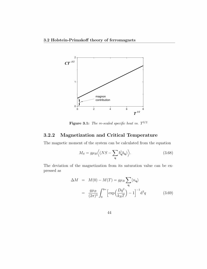
33 Holstein-Primakoff theory of antiferromagnets
with
~ωq = (2JSz)2(1minus γ2q) (3115)
However the explicit calculation of sublattice magnetizations at arbitrarytemperature represents hard and non-trivial mathematical task Neverthe-less at the temperatures that are significantly lower then the Neel transitiontemperature TN one finds that the sublattice magnetization is proportionalto (TTN)
2 The proof of this behavior is left for the reader
54
Chapter 4
Jordan-Wigner Transformationfor the XY Model
In previous parts of this text we have discussed how to apply the bosoniza-tion technique within the Holstein-Primakoff approach to the ferromagneticand antiferromagnetic spin systems In the present chapter we will investi-gate a similar approach which is known as a method of fermioniozation Inparticular we will discuss application of the Wigner-Jordan transformationto the isotropic quantum XY model in order to clarify important points ofthis method
The main idea of this approach is to transform the Hamiltonian de-scribing a spin system by the use of new operators obeying the fermionanticommutation rules
Before we start our analysis it is useful to note that the spectrum of theXY model was exactly found by HBethe [3] in 1931 The Bethersquos approachis of great importance however it is quite involved and rather abstractthus it is difficult to understand even such basic properties as long-rangeorder A much more natural approach to the problem of interacting spin-12 systems was originally introduced in 1928 by Jordan and Wigner [5]
55
41 Jordan-Wigner Transformation for the XY Model
who invented simple mathematical transformations converting spin-12 sys-tems into problems of interacting (and in some cases even non-interacting)spinless fermions In fact the XY model which is a special case of theHeisenberg Hamiltonian reduces to a free theory of spinless fermions un-der the Jordan-Wigner transformations Another reason for choosing theXY model is that the low-energy properties of the full anti-ferromagneticHeisenberg chain such as the presence of gapless excitations and absenceof a long range order are very similar to those of the XY model (see [6] andreferences therein)
We will study a linear chain of N spin-12 atoms interacting antiferro-magnetically with their nearest neighbors This system is described by theHamiltonian
H = JNsumj=1
(Sxj S
xj+1 + Sy
j Syj+1) (41)
where J gt 0 represents the exchange interaction ans Sαi are spin-12 opera-
tors obeying the usual commutation relations (33) As usually we assumecyclic boundary conditions with Sα
N+1 = Sα1 α = x y Of course for
J lt 0 the ferromagnetic case of (41) is obtained Thus if we solve theantiferromagnetic problem exactly then we can immediately obtain alsothe solution of the ferromagnetic XY chain Similarly as in the case ofbozonization we at first introduce spin-raising and spin-lowering operators(313) and rewrite the Hamiltonian as a bilinear form in these operatorsie
H =J
2
Nsumj=1
(Sminusj S
+j+1 + Sminus
j+1S+j ) (42)
It clear that without loss of generality we can set J = 1 in all subsequentcalculations We know that the Splusmn operators belonging to the same siteobey anticommutation relations while that ones on different sites satisfy
56
41 Jordan-Wigner Transformation for the XY Model
usual commutation relations and this mathematical property disables a di-rect diagonalization of (42) The key to the solution of this problem is theJordan-Wigner transformation which enables to obtain the Hamiltonian interms of pure fermion operators
The JordanndashWigner transformation explicitly reads
cdaggern = S+n exp
(minusiπ
nminus1sumj=1
S+j S
minusj
) cn = Sminus
n exp(iπ
nminus1sumj=1
S+j S
minusj
) (43)
and the inverse transformation is given by
S+n = cdaggern exp
(iπ
nminus1sumj=1
cdaggerjcj
) Sminus
n = cn exp(iπ
nminus1sumj=1
cdaggerncn
) (44)
Here it is worth noticing that the signs in the exponents and the order ofthe multipliers in (43) and (44) are not important
The operators cdaggerj ck obey the canonical fermion algebra ie
cj cdaggerk = δjk cdaggerj cdaggerk = 0 cj ck = 0 (45)
To illustrate the mathematics behind we will explicitly prove the first rela-tion while the other anti-commutators in (45) can be computed in a similarfashion
At first we recall the validity of the following relations [S+j Sj S
+k Sk] = 0
[S+j Sj Sk] = minusδjkSk [S
+j Sj S
+k ] = δjkS
+k (S
+j Sj)
2 = S+j Sj since the spin-
raising and spin-lowering operators on different sites commute and on thesame site behave like fermions Therefore
exp(plusmniπ
msumj=n
S+j S
minusj
)=
mprodj=n
exp(plusmniπS+j S
minusj ) (46)
57
41 Jordan-Wigner Transformation for the XY Model
and the exponential function on the rhs of previous equation can be easilyevaluated as follows
exp(plusmniπS+j S
minusj ) =
infinsumk=0
1
k(plusmniπ)k(S+
j Sminusj )
k
= 1 +infinsumk=1
1
k(plusmniπ)kS+
j Sminusj
= 1 + (eplusmniπ minus 1)S+j S
minusj = 1minus 2S+
j Sminusj (47)
Similarly using the following anticommutators
Sminusj 1minus 2S+
j Sminusj = 0 S+
j 1minus 2S+j S
minusj = 0 (48)
one obtains relations[exp
(plusmniπ
msumj=n
S+j S
minusj
) Sminus
k
]=
[exp
(plusmniπ
msumj=n
S+j S
minusj
) S+
k
]= 0 k isin [nm]
(49)
exp
(plusmniπ
msumj=n
S+j S
minusj
) Sminus
k
=
exp
(plusmniπ
msumj=n
S+j S
minusj
) S+
k
= 0 k isin [nm]
(410)
Although all the above calculations have a preparatory character they are ofcrucial importance to demonstrate the fermionic nature of cj and cdaggerk Reallyusing (46)- (410) we can now straightforwardly calculate the following
58
41 Jordan-Wigner Transformation for the XY Model
anti-commutators
cj cdaggerk = Sminusj exp
(iπ
jminus1sumℓ=1
S+ℓ S
minusℓ
)exp
(minusiπ
kminus1sumℓ=1
S+ℓ S
minusℓ
)S+k
+ S+k exp
(minusiπ
kminus1sumℓ=1
S+ℓ S
minusℓ
)exp
(iπ
jminus1sumℓ=1
S+ℓ S
minusℓ
)Sminusj
= Sminusj exp
(iπ
kminus1sumℓ=j
S+ℓ S
minusℓ
)S+k S
+k exp
(iπ
kminus1sumℓ=j
S+ℓ S
minusℓ
)Sminusk
= (Sminusj S
+j minus S+
j Sminusj ) exp
(iπ
kminus1sumℓ=j
S+ℓ S
minusℓ
)= 0 k gt j (411)
In the same way we derive relation
cj cdaggerk = ck cdaggerkdagger = 0 k lt j (412)
ck cdaggerk = Sminusk S
+k + S+
k Sminusk = 1 (413)
Thus we have successfully proved the fermionic commutation relations andnow we can transform the relevant terms in the Hamiltonian
For 1 le j le N minus 1 one obtains
Sminusj S
+j+1 = exp
(minusiπ
jminus1sumℓ=1
cdaggerℓcℓ
)cjc
daggerj+1 exp
(iπ
jsumℓ=1
cdaggerℓcℓ
)= cj exp
(minusiπ
jminus1sumℓ=1
cdaggerℓcℓ
)exp
(iπ
jsumℓ=1
cdaggerℓcℓ
)cdaggerj+1
= cj exp(iπcdaggerjcj)c
daggerj+1 = cj(1minus 2cdaggerjcj)c
daggerj+1
= minus(1minus 2cdaggerjcj)cjcdaggerj+1) = minuscjc
daggerj+1 = cdaggerj+1cj (414)
and similarly we have
Sminusj+1S
+j = (Sminus
j S+j+1)
dagger = cdaggerjcj+1 (415)
59
41 Jordan-Wigner Transformation for the XY Model
Here one should notice that in deriving previous equations we have usedthe following relations
[cdaggerjcj cdaggerkck] = 0 (cdaggerjcj)
2 = cdaggerjcj
[cdaggerjcj ck] = minusδjkck [cdaggerjcj cdaggerk] = minusδjkc
daggerk
1minus 2cdaggerjcj cj = 0 1minus 2cdaggerjcj cdaggerj = 0 (416)
[exp
(plusmniπ
msumj=n
cdaggerjcj
) ck
]=
[exp
(plusmniπ
msumj=n
cdaggerjcj
) cdaggerk
]= 0
k isin [nm] (417)
exp
(plusmniπ
msumj=n
cdaggerjcj
) ck
=
exp
(plusmniπ
msumj=n
cdaggerjcj
) cdaggerk
= 0
k isin [nm] (418)
After expressing the special cyclic boundary term (SminusN S
+1 + Sminus
1 S+N) in
terms of crsquos and substituting Eqs(414) and (415) into Eq(42) we canrewrite the Hamiltonian of the system as
H =1
2
sumj
(cdaggerj+1cj + cdaggerjcj+1) + Hb (419)
where
Hb = minus1
2
(cdagger1cN + cdaggerNc1
)[1 + exp
(plusmniπ
Nsumj=1
cdaggerjcj
)](420)
represents the boundary term which gives an O(Nminus1) contributions to themacroscopic physical quantities and for this reason will be neglected infurther calculations
60
41 Jordan-Wigner Transformation for the XY Model
Applying this simplification we are left with the problem of diagonal-ization of the following bilinear form
H =1
2
sumj
(cdaggerj+1cj + cdaggerjcj+1) (421)
which describes free spinless fermions on a cyclic chain with nearest neighborhopping
In order to diagonalize the Hamiltonian (421) we rewrite it in the form
H =sumjk
cdaggerjAjkck (422)
where the elements of the matrix A are given by
Ajk =1
2(δjk+1 + δkj+1) (423)
Taking into account the translational invariance of the lattice we find theeigenvectors and eigenvalues of A to be
ϕqj =1radicNeiqj Λq = cos(q) (424)
with q = 2πnN
and N2 le n le N2 minus 1 The eigenfunctions ϕqk form anorthonormal and complete set thus we can introduce new operators obeyingthe canonical anticommutation rule
ηq =sumj
ϕlowastqjcj ηdaggerq =
sumj
ϕqjcdaggerj (425)
Using the following inverse transformations
cj =sumq
ϕqjηq cdaggerj =sumq
ϕqjηdaggerq (426)
61
41 Jordan-Wigner Transformation for the XY Model
the Hamiltonian (422) can be rewritten in the diagonal form
H =sumq
Λqηdaggerqηq (427)
Since some of the eigenvalues of A will be negative we perform an additionaltransformation
ξq = ηq Λq ge 0 (428)
ξq = ηdaggerq Λq lt 0 (429)
and obtain
H =sum
qΛqge0
Λqξdaggerqξq +
sumqΛqlt0
Λqξdaggerqξq
=sumqΛq
|Λq|ξdaggerqξq minussum
qΛqlt0
|Λq|
=sumqΛq
|Λq|(ξdaggerqξq minus
1
2
) (430)
Here the ξ operators again obey the canonical anticommutation rulesAs usually the ground state |0⟩ satisfies equation
ξq|0⟩ = 0 forallq (431)
and the operator ξdaggerq generates an elementary fermion excitation with energy|Λq| above the ground state
The dispersion relation for the model under investigation is shown in Fig41 As one can see there always exist gapless excitations near q = plusmnπ2The ground state energy reduced per one spin is given by
U0 =⟨H⟩N
= minus 1
N
sumq
1
2|Λq|
=
int π
π
dq
4π| cos(q)| = minus 1
π
int π2
0
cos(q)dq = minus 1
π(432)
62
41 Jordan-Wigner Transformation for the XY Model
ω(q)
0
02
04
06
08
1
q-20 -15 -10 -05 00 05 10 15 20
Figure 41 Dispersion relation of the XY model
Of course the method of fermionization can been extended to manyother systems including the systems with higher spin and higher spatialdimensions However the analysis of this systems requires complex andtedious calculations and sometimes also the applications additional theo-retical tools methods (for example the Green function technique) that arebeyond the scope of this introductory text
63
Conclusion
Conclusion
In this work we have discussed some theoretical tools that are frequentlyused to investigate the localized quantum spin models
The first approach is the standard mean-field theory which representsthe simplest possible technique usually applied to understand basic quan-titative features of various theoretical models of quantum magnetism Al-though this method is included in many textbooks the formulation is usu-ally very simplified and frequently the authors do not derive the Gibbsfree energy within this method To avoid this problem we have used andelegant formulation based on the Bogolyubov inequality which enables toextend our approach to formulate more accurate theories (for example theOguchi approximation or Constant Coupling Method) One should also em-phasize that in deriving the partition function we have applied the Cauchyintegral formula which enables to calculate exponential function with a ma-trix argument This is an unknown trick which can be used in calculationsin nay branch of theoretical physics
In the Chapter 3 we have discussed the standard spin-wave theory sep-arately for ferromagnetic and antiferromagnetic materials We have shownin detail how to introduce the boson operators that enable to calculate sev-eral physical quantities such as magnetization internal energy and magneticcontribution to the specific heat
The last part is dedicated to the method of fermionization Here we havediscussed the application o Jordan-Wigner transformation to the quantumXY model with spin 12 This approach represent another standard theo-retical approach which is used to investigate quantum magnetism
It is clear from the content of this supporting text that we have coveredjust one special part of quantum theory of magnetism which is howeverdiscussed elementary enough In order to understand further interesting fea-tures of the quantum magnetism it is necessary to study further textbooksfor example [8] [9] [10] [11] )
64
Bibliography
[1] F Bloch Z Physik 61 206 (1930)
[2] T Holstein and H Primakoff Phys Rev 58 1908 (1940)
[3] H Bethe Z Physik 71 205 (1931)
[4] L Hulten Ark Met Asron Fysik 26 A 11 (1938)
[5] P Jordan and E Wigner Z Phys 47 631 (1928)
[6] A Tsvelik Quantum Field Theory in Condensed Matter PhysicsCambridge Cambridge University Press 1995
[7] LJ de Jongh AR Miedema Adv Phys 23 2 (1974)
[8] C Kittel Quantum Theory of Solids New York John Wiley andSons 1987
[9] K Yosida Theory of Magnetism Berlin Springer 1998
[10] P Mohn Magnetism in the Solid State Berlin Springer 2003
[11] N Majlis The Quantum Theory of Magnetism Singapore World Sci-entific 2007
65
41 Jordan-Wigner Transformation for the XY Model
the Hamiltonian (422) can be rewritten in the diagonal form
H =sumq
Λqηdaggerqηq (427)
Since some of the eigenvalues of A will be negative we perform an additionaltransformation
ξq = ηq Λq ge 0 (428)
ξq = ηdaggerq Λq lt 0 (429)
and obtain
H =sum
qΛqge0
Λqξdaggerqξq +
sumqΛqlt0
Λqξdaggerqξq
=sumqΛq
|Λq|ξdaggerqξq minussum
qΛqlt0
|Λq|
=sumqΛq
|Λq|(ξdaggerqξq minus
1
2
) (430)
Here the ξ operators again obey the canonical anticommutation rulesAs usually the ground state |0⟩ satisfies equation
ξq|0⟩ = 0 forallq (431)
and the operator ξdaggerq generates an elementary fermion excitation with energy|Λq| above the ground state
The dispersion relation for the model under investigation is shown in Fig41 As one can see there always exist gapless excitations near q = plusmnπ2The ground state energy reduced per one spin is given by
U0 =⟨H⟩N
= minus 1
N
sumq
1
2|Λq|
=
int π
π
dq
4π| cos(q)| = minus 1
π
int π2
0
cos(q)dq = minus 1
π(432)
62
41 Jordan-Wigner Transformation for the XY Model
ω(q)
0
02
04
06
08
1
q-20 -15 -10 -05 00 05 10 15 20
Figure 41 Dispersion relation of the XY model
Of course the method of fermionization can been extended to manyother systems including the systems with higher spin and higher spatialdimensions However the analysis of this systems requires complex andtedious calculations and sometimes also the applications additional theo-retical tools methods (for example the Green function technique) that arebeyond the scope of this introductory text
63
Conclusion
Conclusion
In this work we have discussed some theoretical tools that are frequentlyused to investigate the localized quantum spin models
The first approach is the standard mean-field theory which representsthe simplest possible technique usually applied to understand basic quan-titative features of various theoretical models of quantum magnetism Al-though this method is included in many textbooks the formulation is usu-ally very simplified and frequently the authors do not derive the Gibbsfree energy within this method To avoid this problem we have used andelegant formulation based on the Bogolyubov inequality which enables toextend our approach to formulate more accurate theories (for example theOguchi approximation or Constant Coupling Method) One should also em-phasize that in deriving the partition function we have applied the Cauchyintegral formula which enables to calculate exponential function with a ma-trix argument This is an unknown trick which can be used in calculationsin nay branch of theoretical physics
In the Chapter 3 we have discussed the standard spin-wave theory sep-arately for ferromagnetic and antiferromagnetic materials We have shownin detail how to introduce the boson operators that enable to calculate sev-eral physical quantities such as magnetization internal energy and magneticcontribution to the specific heat
The last part is dedicated to the method of fermionization Here we havediscussed the application o Jordan-Wigner transformation to the quantumXY model with spin 12 This approach represent another standard theo-retical approach which is used to investigate quantum magnetism
It is clear from the content of this supporting text that we have coveredjust one special part of quantum theory of magnetism which is howeverdiscussed elementary enough In order to understand further interesting fea-tures of the quantum magnetism it is necessary to study further textbooksfor example [8] [9] [10] [11] )
64
Bibliography
[1] F Bloch Z Physik 61 206 (1930)
[2] T Holstein and H Primakoff Phys Rev 58 1908 (1940)
[3] H Bethe Z Physik 71 205 (1931)
[4] L Hulten Ark Met Asron Fysik 26 A 11 (1938)
[5] P Jordan and E Wigner Z Phys 47 631 (1928)
[6] A Tsvelik Quantum Field Theory in Condensed Matter PhysicsCambridge Cambridge University Press 1995
[7] LJ de Jongh AR Miedema Adv Phys 23 2 (1974)
[8] C Kittel Quantum Theory of Solids New York John Wiley andSons 1987
[9] K Yosida Theory of Magnetism Berlin Springer 1998
[10] P Mohn Magnetism in the Solid State Berlin Springer 2003
[11] N Majlis The Quantum Theory of Magnetism Singapore World Sci-entific 2007
65
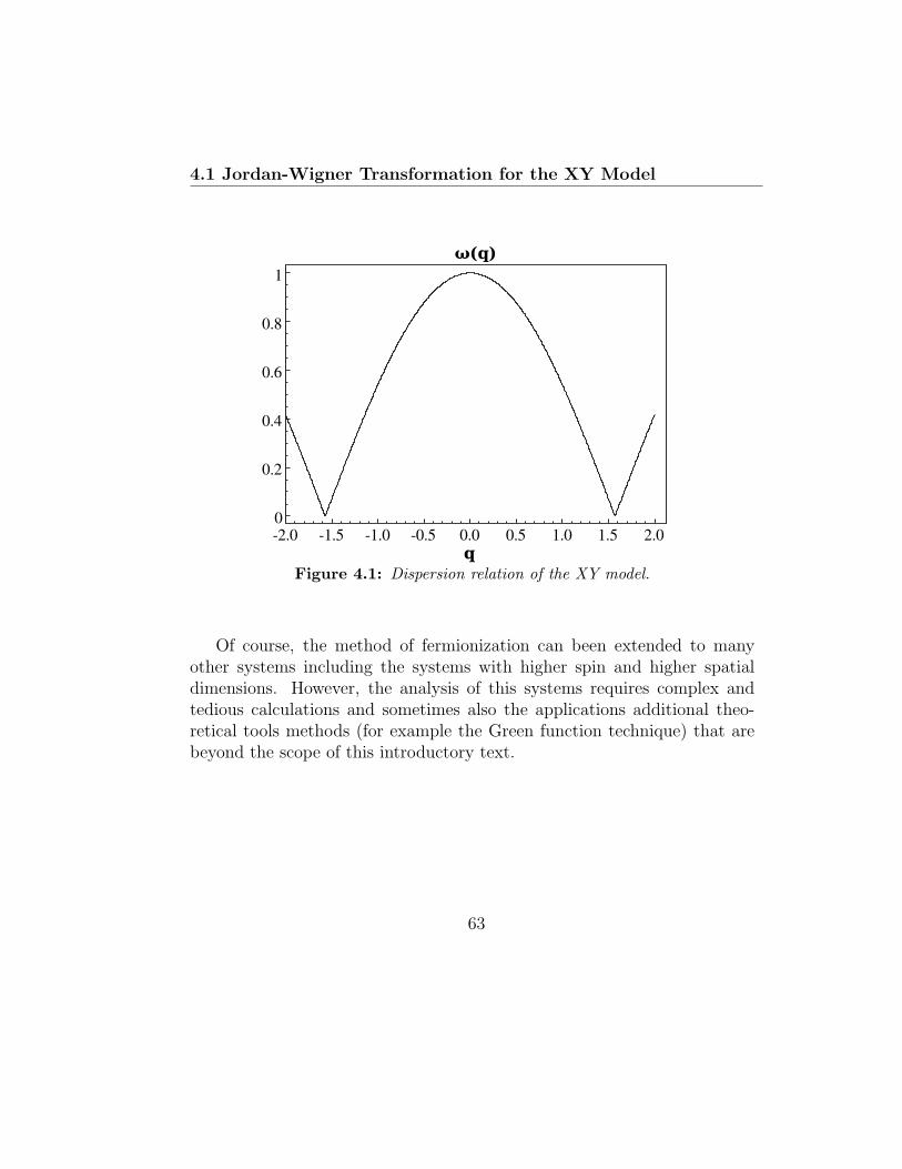
Conclusion
Conclusion
In this work we have discussed some theoretical tools that are frequentlyused to investigate the localized quantum spin models
The first approach is the standard mean-field theory which representsthe simplest possible technique usually applied to understand basic quan-titative features of various theoretical models of quantum magnetism Al-though this method is included in many textbooks the formulation is usu-ally very simplified and frequently the authors do not derive the Gibbsfree energy within this method To avoid this problem we have used andelegant formulation based on the Bogolyubov inequality which enables toextend our approach to formulate more accurate theories (for example theOguchi approximation or Constant Coupling Method) One should also em-phasize that in deriving the partition function we have applied the Cauchyintegral formula which enables to calculate exponential function with a ma-trix argument This is an unknown trick which can be used in calculationsin nay branch of theoretical physics
In the Chapter 3 we have discussed the standard spin-wave theory sep-arately for ferromagnetic and antiferromagnetic materials We have shownin detail how to introduce the boson operators that enable to calculate sev-eral physical quantities such as magnetization internal energy and magneticcontribution to the specific heat
The last part is dedicated to the method of fermionization Here we havediscussed the application o Jordan-Wigner transformation to the quantumXY model with spin 12 This approach represent another standard theo-retical approach which is used to investigate quantum magnetism
It is clear from the content of this supporting text that we have coveredjust one special part of quantum theory of magnetism which is howeverdiscussed elementary enough In order to understand further interesting fea-tures of the quantum magnetism it is necessary to study further textbooksfor example [8] [9] [10] [11] )
64
Bibliography
[1] F Bloch Z Physik 61 206 (1930)
[2] T Holstein and H Primakoff Phys Rev 58 1908 (1940)
[3] H Bethe Z Physik 71 205 (1931)
[4] L Hulten Ark Met Asron Fysik 26 A 11 (1938)
[5] P Jordan and E Wigner Z Phys 47 631 (1928)
[6] A Tsvelik Quantum Field Theory in Condensed Matter PhysicsCambridge Cambridge University Press 1995
[7] LJ de Jongh AR Miedema Adv Phys 23 2 (1974)
[8] C Kittel Quantum Theory of Solids New York John Wiley andSons 1987
[9] K Yosida Theory of Magnetism Berlin Springer 1998
[10] P Mohn Magnetism in the Solid State Berlin Springer 2003
[11] N Majlis The Quantum Theory of Magnetism Singapore World Sci-entific 2007
65