Factorization Machine and RecommendationSystems

Tzviel Frostig

November 30, 2019

1/42

Table of contents

2/42

Factorization Machines

Recommendation systems and Matrix Factorization methods

I Matrix Factorization Techniques for Recommender Systems -Yehuda Koren, Robert Bell and Chris Volinsky (2009)

I Factorization Meets the Neighborhood: a MultifacetedCollaborative Filtering Model- Yehuda Koren (2008)

Factorization Machines

I Factorization Machines - Steffen Rendle (2010)

I Factorization Machines with libfm - Steffen Rendle (2012)

3/42

Part I

Introduction

4/42

Papers for Talk

I A recommendation system goal is to predict a user responseto various options

I Common machine learning task, used in: music and videoplaylist generators, product recommendations, online dating,restaurants and more

I Data of typical problem is characterized by large amount ofmissing values

I A hard problem

5/42

Netflix Prize

I In 2006, Netflix offered a prize of 1m$ to whoever couldimprove their user prediction algorithm by 10%

I The competing teams were given a data set of 480k users and18K movie, most of it empty

I The prize was finally won at 2009 using methods based onMatrix Factorization

6/42

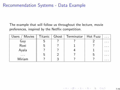
Recommendation Systems - Data Example

The example that will follow us throughout the lecture, moviepreferences, inspired by the Netflix competition.

Users / Movies Titanic Ghost Terminator Hot Fuzz . . .

Guy 5 ? ? 2 . . .Roei 5 ? 1 ? . . .Ayala ? ? 4 1 . . .. . . 5 2 ? 5 . . .

Miriam ? 3 ? ? . . .

7/42

Recommendation Systems

Recommendation systems are based on one of two strategies:

I Content Based - Create a profile for each user or product tocharacterize it. Recommend a product according to theattributes.

I Collaborative Filtering - A method of making prediction(filtering) about interests of the user by collection preferencefrom many users (collaborating).

1. Neighborhood based approach (find similar users, K-NN forexample)

2. Latent factor methods, (find some hidden structure in thedata)

8/42

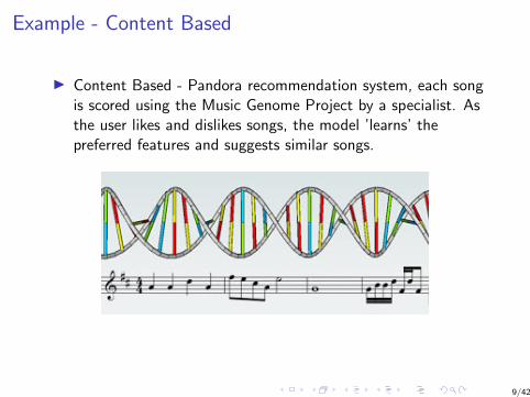
Example - Content Based

I Content Based - Pandora recommendation system, each songis scored using the Music Genome Project by a specialist. Asthe user likes and dislikes songs, the model ’learns’ thepreferred features and suggests similar songs.

9/42

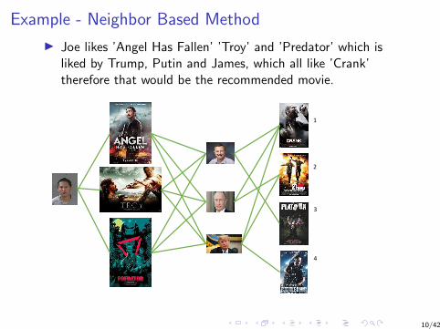
Example - Neighbor Based Method

I Joe likes ’Angel Has Fallen’ ’Troy’ and ’Predator’ which isliked by Trump, Putin and James, which all like ’Crank’therefore that would be the recommended movie.

1

2

3

4

10/42

Latent Factor Method

I Find k , k << p latent factors which characterize items andusers, the factors correspond to the music Genes.

I The latent factors can be for example comedy vs drama,amount of action and the like.

I For users, each factor measures how much the user likesmovies that score high on the corresponding movie factor.

11/42

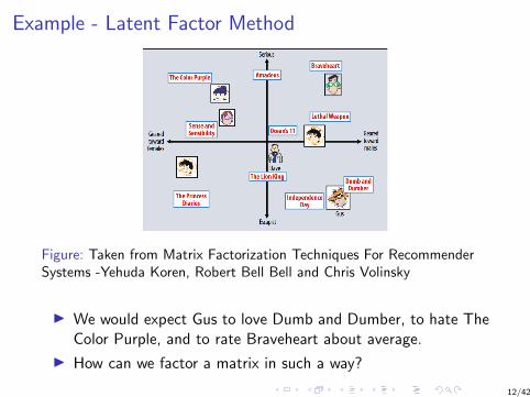
Example - Latent Factor Method

Figure: Taken from Matrix Factorization Techniques For RecommenderSystems -Yehuda Koren, Robert Bell Bell and Chris Volinsky

I We would expect Gus to love Dumb and Dumber, to hate TheColor Purple, and to rate Braveheart about average.

I How can we factor a matrix in such a way?

12/42

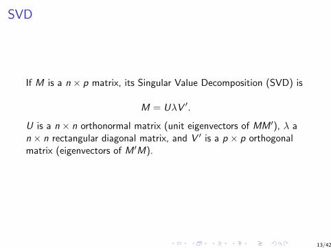
SVD

If M is a n × p matrix, its Singular Value Decomposition (SVD) is

M = UλV ′.

U is a n × n orthonormal matrix (unit eigenvectors of MM ′), λ an × n rectangular diagonal matrix, and V ′ is a p × p orthogonalmatrix (eigenvectors of M ′M).

13/42

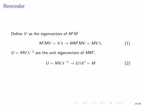
Reminder

Define V as the eigenvectors of M ′M

M ′MV = Vλ→ MM ′MV = MVλ. (1)

U = MVλ−1 are the unit eigenvectors of MM ′,

U = MVλ−1 → UλV ′ = M (2)

14/42

SVD & PCA

I As statistician we are more familiar with Principle ComponentAnalysis (PCA)

I Note that PCA is SVD for M ′ and M

M ′M = VλU ′UλV ′ → M ′M = Vλ2V

15/42

SVD - Example For Dimensionality Reduction

I Can SVD be used to for dimensionality reduction?

I A lower rank matrix factorization cant be found, by removingvectors which contribute little to the explained variance

16/42

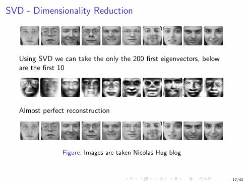
SVD - Dimensionality Reduction

Using SVD we can take the only the 200 first eigenvectors, beloware the first 10

Almost perfect reconstruction

Figure: Images are taken Nicolas Hug blog

17/42

SVD for Recommendation Systems

I U columns can be viewed as the various typical user

I V columns can be viewed as the various typical movies

I λ can be viewed as how prevalent is the combination ofspecific typical movie and user

I Seems suitable for our problem, can we use it for ourrecommendation problem?

18/42

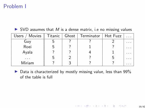
Problem I

I SVD assumes that M is a dense matrix, i.e no missing values

Users / Movies Titanic Ghost Terminator Hot Fuzz . . .

Guy 5 ? ? 2 . . .Roei 5 ? 1 ? . . .Ayala ? ? 4 1 . . .. . . 5 2 ? 5 . . .

Miriam ? 3 ? ? . . .

I Data is characterized by mostly missing value, less than 99%of the table is full

19/42

Solution I - Imputation

What wrong with imputation?

I Computationally expensive, as the most of the entries of thematrix are missing

I It can distort the data

20/42

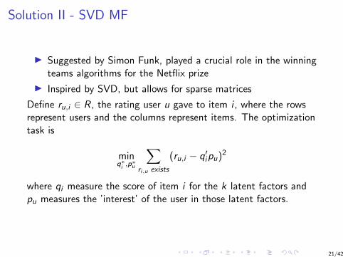
Solution II - SVD MF

I Suggested by Simon Funk, played a crucial role in the winningteams algorithms for the Netflix prize

I Inspired by SVD, but allows for sparse matrices

Define ru,i ∈ R, the rating user u gave to item i , where the rowsrepresent users and the columns represent items. The optimizationtask is

minq∗i ,p

∗u

∑ri,u exists

(ru,i − q′ipu)2

where qi measure the score of item i for the k latent factors andpu measures the ’interest’ of the user in those latent factors.

21/42

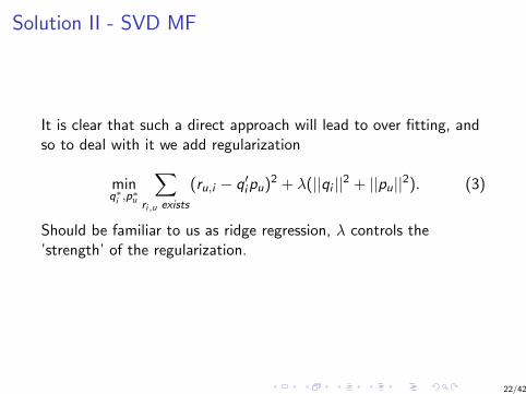
Solution II - SVD MF

It is clear that such a direct approach will lead to over fitting, andso to deal with it we add regularization

minq∗i ,p

∗u

∑ri,u exists

(ru,i − q′ipu)2 + λ(||qi ||2 + ||pu||2). (3)

Should be familiar to us as ridge regression, λ controls the’strength’ of the regularization.

22/42

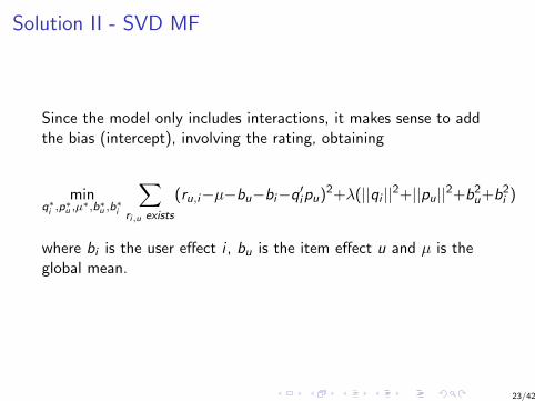
Solution II - SVD MF

Since the model only includes interactions, it makes sense to addthe bias (intercept), involving the rating, obtaining

minq∗i ,p

∗u ,µ

∗,b∗u ,b∗i

∑ri,u exists

(ru,i−µ−bu−bi−q′ipu)2+λ(||qi ||2+||pu||2+b2u+b2i )

where bi is the user effect i , bu is the item effect u and µ is theglobal mean.

23/42

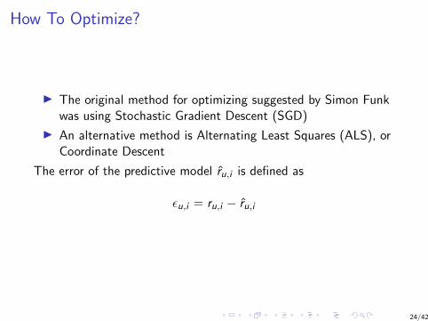
How To Optimize?

I The original method for optimizing suggested by Simon Funkwas using Stochastic Gradient Descent (SGD)

I An alternative method is Alternating Least Squares (ALS), orCoordinate Descent

The error of the predictive model ru,i is defined as

εu,i = ru,i − ru,i

24/42

SGD

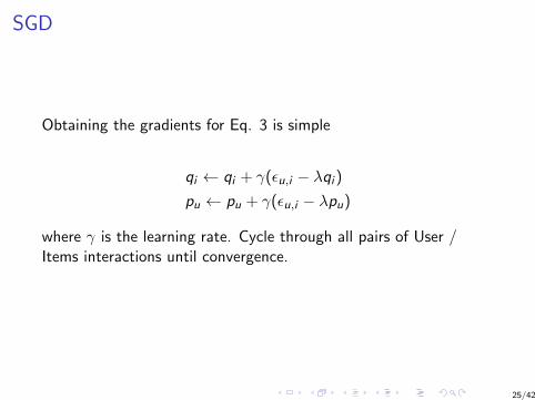
Obtaining the gradients for Eq. 3 is simple

qi ← qi + γ(εu,i − λqi )pu ← pu + γ(εu,i − λpu)

where γ is the learning rate. Cycle through all pairs of User /Items interactions until convergence.

25/42

ALS

I If qi or pu were known, Eq. 3 was convex and could be solvedusing least squares

I Alternating between pu and qi , at each iteration solving usingleast square ensures a decrease of the loss and eventuallyconvergence

I Since each qi and pu are obtained individually, it is easy toparallelize.

26/42

Summary

I SVD- MF offers a reasonable method to model User - Iteminteractions

I Two simple algorithms for optimization

I Whats missing?

27/42

Cold Start Problem

From Wikipidea

”Cold start is a potential problem in computer-based informationsystems which involve a degree of automated data modeling.Specifically, it concerns the issue that the system cannot draw anyinferences for users or items about which it has not yet gatheredsufficient information.”

I What happens when a user supply very few ratings, how canwe predict his/her preference?

28/42

Implicit Preferences

I In many cases we have additional information regarding theusers, in the Netflix data, we could have not only the ratedmovies but also the history of rented videos

I The data is not limited to implicit preferences, but also toinformation such as demographics

I Define xi ∈ N(u), |xi | = k the set of items for which user ushowed implicit preference, pu ∈ R(u) the explicit preferencesof the user and ya ∈ A(u), |ya| = k is the set of attributes thatdescribe a user

29/42

SVD++

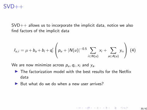
SVD++ allows us to incorporate the implicit data, notice we alsofind factors of the implicit data

ru,i = µ+bu +bi +q′i

pu + |N(u)|−0.5∑

i∈N(u)

xi +∑

a∈A(u)

yα

(4)

We are now minimize across pu, qi , xi and ya.

I The factorization model with the best results for the Netflixdata

I But what do we do when a new user arrives?

30/42

Asymmetric SVD

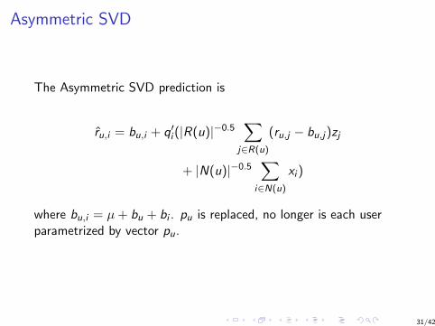
The Asymmetric SVD prediction is

ru,i = bu,i + q′i (|R(u)|−0.5∑

j∈R(u)

(ru,j − bu,j)zj

+ |N(u)|−0.5∑

i∈N(u)

xi )

where bu,i = µ+ bu + bi . pu is replaced, no longer is each userparametrized by vector pu.

31/42

Asymmetric SVD - Benefits

I Since Asymmetric-SVD does not parameterize users, we canhandle new users as soon as they provide feedback to thesystem, without needing to re-train the model and estimatenew parameters. For new items we do need to re-train themodel.

I Integration of implicit data, similar to SVD++ takes intoaccount additional information regarding the user

32/42

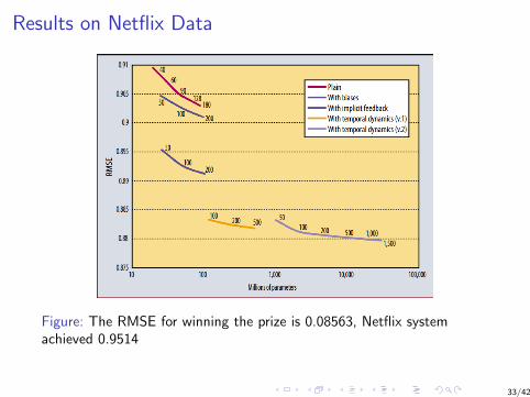
Results on Netflix Data

Figure: The RMSE for winning the prize is 0.08563, Netflix systemachieved 0.9514

33/42

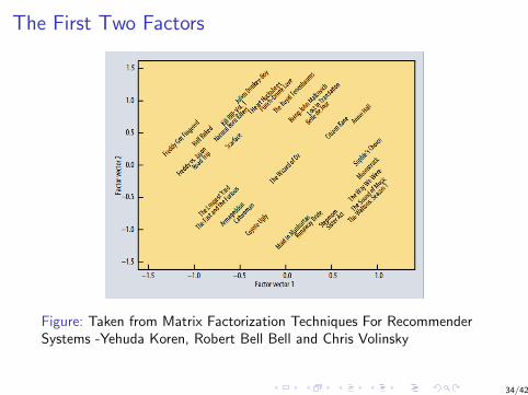
The First Two Factors

Figure: Taken from Matrix Factorization Techniques For RecommenderSystems -Yehuda Koren, Robert Bell Bell and Chris Volinsky

34/42

Are we done?

I There are many other models each incorporate additionalinformation, such as confidence level, temporal dynamics andmore, each requires to create the data matrix in a specific way

I It seems that for each scenario one should use a specializedalgorithm

35/42

Part II

Factorization Machines

36/42

Factorization Machines

I Suggested by Steffen Rendle (2010)

I Successful in tasks such as collaborative filtering and click rateprediction

I Implemented in a few python packages, tesnorFlow and libFM

37/42

Factorization Machines

I A general predictor, can be used for classification, regressionand ranking

I Generalizes Factorization Models, mostly used inrecommendation systems

I Model based

I Linear in time

38/42

Factorization Machines

I A general predictor, can be used for classification, regressionand ranking

I Generalizes Factorization Models, mostly used inrecommendation systems

I Linear in time

I In the words of the author ”.. combines the advantages ofSupport Vector Machines (SVM) with factorization models”

39/42

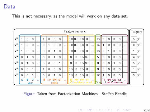
Data

This is not necessary, as the model will work on any data set.

Figure: Taken from Factorization Machines - Steffen Rendle

40/42

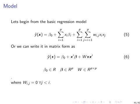
Model

Lets begin from the basic regression model

y(x) = β0 +

p∑i=1

xiβi +

p∑i=1

p∑j=i+1

wi ,jxixj (5)

Or we can write it in matrix form as

y(x) = β0 + x′β + W xx

′ (6)

β0 ∈ R β ∈ Rp W ∈ Rp×p

.where Wi ,j = 0 ∀j < i .

41/42

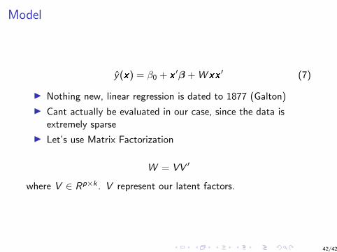
Model

y(x) = β0 + x′β + W xx

′ (7)

I Nothing new, linear regression is dated to 1877 (Galton)

I Cant actually be evaluated in our case, since the data isextremely sparse

I Let’s use Matrix Factorization

W = VV ′

where V ∈ Rp×k . V represent our latent factors.

42/42

Model

y(x) = β0 + x′β + W xx

′ (8)

I Nothing new, linear regression is dated to 1877 (Galton)

I Cant actually be evaluated in our case, since the data isextremely sparse

I Let’s use Matrix Factorization

W = VV ′

where V ∈ Rp×k . V represent our latent factors.

43/42