Embed Size (px)
Citation preview
Faceless Person Recognition;Privacy Implications in Social Media
Seong Joon Oh, Rodrigo Benenson, Mario Fritz, Bernt Schiele
Max-Planck Institute for Informatics{joon, benenson, mfritz, schiele}@mpi-inf.mpg.de
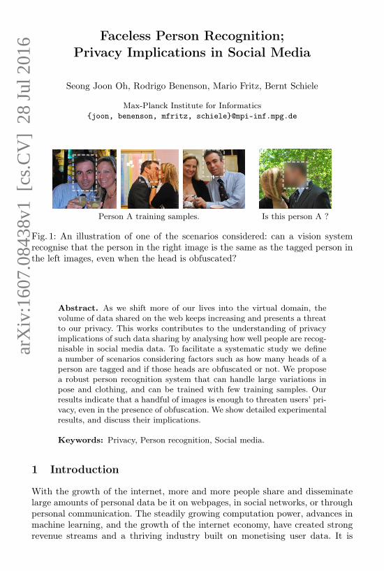
Person A training samples. Is this person A ?
Fig. 1: An illustration of one of the scenarios considered: can a vision systemrecognise that the person in the right image is the same as the tagged person inthe left images, even when the head is obfuscated?
Abstract. As we shift more of our lives into the virtual domain, thevolume of data shared on the web keeps increasing and presents a threatto our privacy. This works contributes to the understanding of privacyimplications of such data sharing by analysing how well people are recog-nisable in social media data. To facilitate a systematic study we definea number of scenarios considering factors such as how many heads of aperson are tagged and if those heads are obfuscated or not. We proposea robust person recognition system that can handle large variations inpose and clothing, and can be trained with few training samples. Ourresults indicate that a handful of images is enough to threaten users’ pri-vacy, even in the presence of obfuscation. We show detailed experimentalresults, and discuss their implications.
Keywords: Privacy, Person recognition, Social media.
1 Introduction
With the growth of the internet, more and more people share and disseminatelarge amounts of personal data be it on webpages, in social networks, or throughpersonal communication. The steadily growing computation power, advances inmachine learning, and the growth of the internet economy, have created strongrevenue streams and a thriving industry built on monetising user data. It is
arX
iv:1
607.
0843
8v1
[cs
.CV
] 2
8 Ju
l 201
6
2 Oh et al.
clear that visual data contains private information, yet the privacy implicationsof this data dissemination are unclear, even for computer vision experts. We areaiming for a transparent and quantifiable understanding of the loss in privacyincurred by sharing personal data online, both for the uploader and other userswho appear in the data.
In this work, we investigate the privacy implications of disseminating photosof people through social media. Although social media data allows to identifya person via different data types (timeline, geolocation, language, user profile,etc.) [1], we focus on the pixel content of an image. We want to know how wella vision system can recognise a person in social photos (using the image contentonly), and how well users can control their privacy when limiting the number oftagged images or when adding varying degrees of obfuscation (see figure 1) totheir heads.
An important component to extract maximal information out of visual datain social networks is to fuse different data and provide a joint analysis. Wepropose our new Faceless Person Recogniser (described in §5), which not onlyreasons about individual images, but uses graph inference to deduce identitiesin a group of non-tagged images. We study the performance of our system onmultiple privacy sensitive user scenarios (described in §3), analyse the mainresults in §6, and discuss implications and future work in §7. Since we focuson the image content itself, our results are a lower-bound on the privacy lossresulting from sharing such images.Our contributions are:
– We discuss dimensions that affect the privacy of online photos, and definea set of scenarios to study the question of privacy loss when social mediaimages are aggregated and processed by a vision system.
– We propose our new Faceless Person Recogniser, which uses convnet featuresin a graphical model for joint inference over identities.
– We study the interplay and effectiveness of obfuscation techniques with re-gard of our vision system.
2 Related work
Nowadays, essentially all online activities can be potentially used to identify aninternet user [1]. Privacy of users in social network is a well studied topic in thesecurity community [2, 3, 1, 4]. There are works which consider the relationshipbetween privacy and photo sharing activities [5, 6], yet they do not performquantitative studies.
Camera recognition. Some works have shown that it is possible to identify thecamera taking the photos (and thus link photos and events via the photogra-pher), either from the file itself [7] or from recognisable sensing noise [8, 9]. Inthis work we focus exclusively on the image content, and leave the exploita-tion of image content together with other forms of privacy cues (e.g. additionalmeta-data from the social network) for future work.
Faceless Person Recognition 3
Image types. Most previous work on person recognition in images has focusedeither on face images [10] (mainly frontal head) or on the surveillance scenario[11, 12], where the full body is visible, usually in low resolution. Like other areasof computer vision, the last years have seen a shift from classifiers based on hand-crafted features and metric learning approaches [13, 14, 15, 16, 17, 18, 19] towardsmethods based on deep learning [20, 21, 22, 23, 24, 25, 26, 27]. Different from facerecognition and surveillance scenarios, the social network images studied heretend to show a diverse range of poses, activities, points of view, scenes (indoors,outdoors), and illumination. This increased diversity makes recognition morechallenging and only a handful of works have addressed explicitly this scenario[28, 29, 30]. We construct our experiments on top of the recently introducedPIPA dataset [29], discussed in §4.
Recognition tasks. The notion of “person recognition” encompasses multiple re-lated problems [31]. Typical “person recognition” considers a few training samplesover many different identities, and a large test set. It is thus akin to fine grainedcategorization. When only one training sample is available and many test images(typical for face recognition and surveillance scenarios [10, 12, 32]), the problemis usually named “re-identification”, and it becomes akin to metric learning orranking problems. Other related tasks are, for example, face clustering [33, 26],finding important people [34], or associating names in text to faces in images[35, 36]. In this work we focus on person recognition with on average 10 trainingsamples per identity (and hundreds of identities), as in typical social networkscenario.
Cues. Given a rough bounding box locating a person, different cues can be usedto recognise a person. Much work has focused on the face itself ([20, 21, 22,23, 24, 25, 26, 27, 37] to name a few recent ones). Pose-independent descriptorshave been explored for the body region [28, 38, 39, 29, 30]. Various other cueshave been explored, for example: attributes classification [40, 41], social context[42, 43], relative camera positions [44], space-time priors [45], and photo-albumpriors [46]. In this work, we build upon [30] which fuses multiple convnet cuesfrom head, body, and the full scene. As we will discuss in the following sections,we will also indirectly use photo-album information.
Identify obfuscation. Some previous works have considered the challenges of de-tection and recognition under obfuscation (e.g. see figure 1). Recently, [47] quan-tified the decrease in Facebook face detection accuracy with respect to differenttypes of obfuscation, e.g. blur, blacking-out, swirl, and dark spots. However, onprinciple, obfuscation patterns can expose faces at a higher risk of detection bya fine-tuned detector (e.g. blur detector). Unlike their work, we consider theidentification problem with a system adapted to obfuscation patterns. Similarly,a few other works studied face recognition under blur [48, 49]. However, to thebest of our knowledge, we are the first to consider person recognition under headobfuscation using a trainable system that leverages full-body cues.
4 Oh et al.
3 Privacy scenarios
Fully visible Gaussian blur
Black fill-in White fill-in
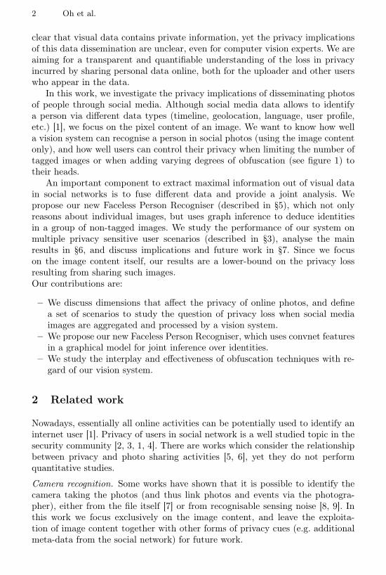
Fig. 2: Obfuscation types consid-ered.
We consider a hypothetical social photosharing service user. The user has a setof photos of herself and others in her ac-count. Some of these photos have identitytags and the others do not have such iden-tity tags. We assume that all heads on thetest photos have been detected, either byan automatic detection system, or becausea user is querying the identity of a specifichead. Note that we do not assume that thefaces are visible nor that persons are ina frontal-upstanding pose. A “tag” is anassociation between a given head and aunique identifier linked to a specific iden-tity (social media user profile).
Goal. The task of our recognition systemis to identify a person of interest (marked
via its head bounding box), by leveraging all the photos available (both with andwithout identity tags). In this work, we want to explore how effective differentstrategies are to protect the user identity.
We consider four different dimensions that affect how hard or easy it is torecognise a user:
Number of tagged heads. We vary the number of tagged images available peridentity. The more tagged images available, the easier it should be to recognisesomeone in new photos. In the experiments of §5 & §6 we consider that 1∼ 10tagged images are available per person.
Obfuscation type. Users concerned with their privacy might take protectivemeasures by blurring or masking their heads. Other than the fully visible case(non-obfuscated), we consider three other obfuscations types, shown in figure 2.We consider both black and white, since [47] showed that commercial systemsmight react differently to these. The blurring parameters are chosen to resemblethe YouTube face blur feature.
Amount of obfuscation. Depending on the user’s activities (and her friendsposting photos of her), not all photos might be obfuscated. We consider a variablefraction of these.

Faceless Person Recognition 5
Table 1: Privacy scenarios considered. Each row in the table can be appliedfor the “across events” and “within events” case, and over different obfusca-tion types. See text §3. The obfuscation fraction indicates tagged/non-taggedheads. Bold abbreviations are reused in follow-up figures. In scenario Sτ1 ,τ ∈ {1.25, 2.5, 5, 10}.
Abbre-viation Brief description Amount of
tagged headsAmount of
obfuscated headsS0 Privacy indifferent 100% 0%Sτ1 Some of my images are tagged τ instances 0%S2 One non-tagged head is obfuscated 10 instances 0%/1 instanceS3 All my heads are obfuscated 10 instances 100%S′3 All tagged heads are obfuscated 10 instances 100%/0%
S′′3 All non-tagged heads are obfuscated 10 instances 0%/100%
Domain shift. For the recognition task, there is a difference if all photos belongto the same event, where the appearance of people change little; or if the set ofphotos without tags correspond to a different event than the ones with identitytags. Recognising a person when the clothing, context, and illumination havechanged (“across events”) is more challenging than when they have not (“withinevents”).
Based on these four dimensions, we discuss a set of scenarios, summarised intable 1. Clearly, these only cover a subset of all possible combinations along thementioned four dimensions. However, we argue that this subset covers importantand relevant aspects for our exploration on privacy implications.
Scenario S0. Here all heads are fully visible and tagged. Since all heads aretagged, the user is fully identifiable. This is the classic case without anyprivacy.
Scenario S1. There is no obfuscation but not all images are tagged. This isthe scenario commonly considered for person recognition, e.g. [28, 29, 30].Unless otherwise specified we use S10
1 , where an average of 10 instances of theperson are tagged (average across all identities). This is a common scenariofor social media users, where some pictures are tagged, but many are not.
Scenario S2. Here the user has all of her heads visible, except for the one non-tagged head being queried. This would model the case where the user wantsto conceal her identity in one particular published photo.
Scenario S3. The user aims at protecting her identity by obfuscating all herheads (using any obfuscation type, see figure 2). Both tagged and non-taggedheads are obfuscated. This scenario models a privacy concerned user. Notethat the body is still visible and thus usable to recognise the user.
Scenarios S′3&S′′3 . These consider the case of a user that inconsistently usesthe obfuscation tactic to protect her identity. Albeit on the surface theseseems like different scenarios, if the visual information of the heads cannotbe propagated from/to the tagged/non-tagged heads, then these are func-tionally equivalent to S3.

6 Oh et al.
Each of these scenarios can be applied for the “across/within events” dimension.In the following sections we will build a system able to recognise persons acrossthese different scenarios, and quantify the effect of each dimension on the recog-nition capabilities (and thus their implication on privacy). For our system, thetagged heads become training data, while the non-tagged heads are used as testdata.
4 Experimental setup
We investigate the scenarios proposed in §3 through a set of controlled exper-iments on a recently introduced social media dataset: PIPA (People In PhotoAlbums) [29]. In this section, we project the scenarios in §3 onto specific aspectsof the PIPA dataset, describing how much realism can be achieved and what arepossible limitations.
PIPA dataset. The PIPA dataset [29] consists of annotated social media photoson Flickr. It contains ∼40k images over ∼2k identities, and captures subjects ap-pearing in diverse social groups (e.g. friends, colleagues, family) and events (e.g.conference, vacation, wedding). Compared to previous social media datasets,such as [28] (∼ 600 images, 32 identities), PIPA presents a leap both in size anddiversity. The heads are annotated with a bounding box and an identity tag.The individuals appear in diverse poses, point of view, activities, sceneries, andthus cover an interesting slice of the real world. See examples in [29, 30], as wellas figures 1 and 14.One possible limitation of the dataset, is that only repeating identities have beenannotated (i.e. a subset of all persons appearing in the images). However, with atest set covering ∼13k instances over ∼600 identities (∼20 instances/identity),it still presents a large enough set of identities to enable an interesting studyand derive relevant conclusions. We believe PIPA is currently the best publicdataset for studying questions regarding privacy in social media photos.
Albums. From the Flickr website, each photo is associated with an album iden-tifier. The ∼ 13k test instances are grouped in ∼ 8k photos belonging to ∼ 350albums. We use the photo album information indirectly during our graph infer-ence (§5.3).
Protocol. The PIPA dataset defines train, validation, and test partitions (∼17k,∼ 5k, ∼ 8k photos respectively), each containing disjoint sets of identities [29].The train partition is used for convnet training. The validation data is usedfor component-wise evaluation of our system, and the test set for drawing finalconclusions. The validation and test partitions are further divided into split0and split1. Each split0/1 contains half of the instances for each identity in thevalidation and test sets (∼10 instances/identity per split, on average).
Splits. When instantiating the scenarios from §3, the tagged faces are all part ofsplit0. In S1, S2, and S3, split1 is never tagged. The task of our Faceless PersonRecognition System is to recognise every query instance from split1, possiblyleveraging other non-tagged instances in split1.
Faceless Person Recognition 7
Domain shift. Other than the one split defined in [29], [30] proposed additionalsplits with increasing recognition difficulty. We use the “Original” split as a goodproxy for the “within events” case, and the “Day” split for “across events”. In theday split, split0 and split1 contain images of a given person across different days.
5 Faceless Recognition System
In this section, we introduce the Faceless Recognition System to study the effec-tiveness of privacy protective measures in §3. We choose to build our own baselinesystem, as opposed to using an existing system as in [47], for adaptibility of thesystem to obfuscation and reproducibility for future research.
Our system does joint recognition employing a conditional random field(CRF) model. CRF often used for joint recognition problems in computer vision[42, 43, 50, 51]. It enables the communication of information across instances,strengthening weak individual cues. Our CRF model is formulated as follows:
argmaxY
1
|V |∑i∈V
φθ(Yi|Xi) +α
|E|∑
(i, j)∈E
1[Yi=Yj ]ψθ(Xi, Xj) (1)
with observations Xi, identities Yi and unary potentials φθ(Yi|Xi) defined oneach node i ∈ V (detailed in §5.1) as well as pairwise potentials ψθ(Xi, Xj)defined on each edge (i, j) ∈ E (detailed in §5.2). 1[·] is the indicator function,and α > 0 controls the unary-pairwise balance.
Unary. We build our unary φθ upon a state of the art, publicly available personrecognition system, naeil [30]. The system was shown to be robust to decreasingnumber of tagged examples. It uses not only the face but also context (e.g. bodyand scene) as cues. Here, we also explore its robustness to obfuscation, see §5.1.
Pairwise. By adding pairwise terms over the unaries, we expect that the systemto propagate predictions across nodes (instances). When a unary prediction isweak (e.g. obfuscated head), the system aggregates information from connectednodes with possibly stronger predictions (e.g. visible face), and thus deduce thequery identity. Our pairwise term ψθ is a siamese network build on top of theunary features, see §5.2.
Experiments on the validation set indicate that, for all scenarios, the per-formance improves with increasing values of α, and reaches the plateau aroundα = 102. We use this value for all the experiments and analysis.
In the rest of the section, we provide a detailed description of the differentparts and evaluate our system component-wise.
5.1 Single person recognition
We build our single person recogniser (the unary potential φθ of the CRF model)upon the state of the art person recognition system naeil [30].
First, 17 AlexNet [52] cues are extracted and concatenated from multipleregions (head, body, and scene) defined relative to the ground truth head boxes.
8 Oh et al.
Visible
Blur
Black
White
Naive
baseline
0
20
40
60
80
100accuracy
(a) Within eventsVisible
Blur
Black
White
Naive
baseline
accuracy
0
20
40
60
80
100visible
non-adapted
adapted
naive baseline
(b) Across events
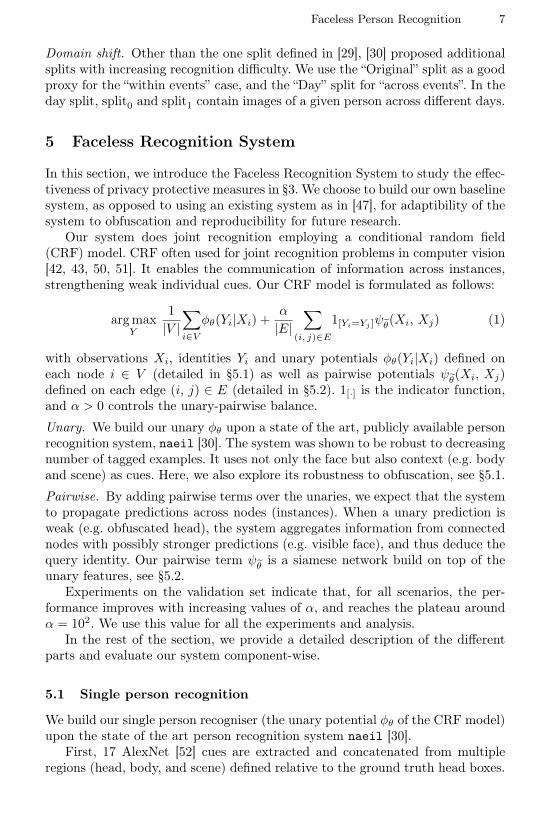
Fig. 3: Impact of head obfuscation on our unary term. Compared to visible (unob-fuscated) case, it struggles on obfuscations (blur, black, and white); nonetheless,it is still far better than the naive baseline classifier that blindly predicts the mostpopular class. “Adapted” means CNN models are trained for the correspondingobfuscation type.
We then train per-identity logistic regression models on top of the resulting4096× 17 dimensional feature vector, which constitute the φθ(·|Xi) vector.
The AlexNet models are trained on the PIPA train set, while the logisticregression weights are trained on the tagged examples (split0). For each obfus-cation case, we also train new AlexNet models over obfuscated images (referredto as “adapted” in figure 3). We assume that at test time the obfuscation can beeasily detected, and the appropriate model is used. We always use the “adapted”model unless otherwise stated.
Figures 3 and 4 evaluate our unary term over the PIPA validation set, underdifferent obfuscation, within/across events, and with varying number of train-ing tags. In the following, we discuss our main findings on how single personrecognition is affected by these measures.
Adapted models are effective for blur. When comparing “adapted” to “non-adapted”in figure 3, we see that adaptation of the convnet models is overall positive. Itmakes minor differences for black or white fill-in, but provides a good boost inrecognition accuracy for the blur case, especially in the across events case (5+percent points gain).
Robustness to obfuscation. After applying black obfuscation in the within eventscase, our unary performs only slightly worse (from “visible” 91.5% to “blackadapted” 80.9%). This is 80 times better than a naive baseline classifier (1.04%)that blindly predicts the most popular class. In the across events case, the “visi-ble” performance drops from from 47.4% to 14.7%, after black obfuscation, whichis still more than 3 times accurate than the naive baseline (4.65%).
Black and white fill-in have similar effects. [47] suggests that white fill-in con-fuses a detection system more than does the black. In our recognition setting,black and white fill-in have similar effects: 80.9% and 79.6% respectively, for
Faceless Person Recognition 9
#tagged examples/person
0
20
40
60
80
100Accuracy
1.25 2.5 5 10
VisibleBlurBlackWhite
(a) Across Events#tagged examples/person
0
20
40
60
80
100
Accuracy
1.25 2.5 5 10
VisibleBlurBlackWhite
(b) Across Events
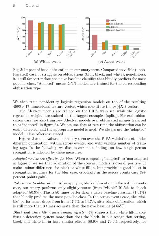
Fig. 4: Single person recogniser at different tag rates.
Correct pair
Incorrect pair
Fig. 5: Matchingin social media.
within events, adapted case (see figure 3). Thus, we omit the experiments forwhite fill-in obfuscation in the next sections.
The system is robust to small number of tags. As shown in figure 4 the singleperson recogniser is robust to a small number of identity tags. For example,in the within events, visible case, it performs at 69.9% accuracy even at 1.25instances/identity tag rate, while using 10 instances/identity it achieves 91.5%.
5.2 Person pair matching
In this section, we introduce a method for predicting matches between a pairof persons based on head and body cues. This is the pairwise term in our CRFformulation (equation 2). Note that person pair matching in social media contextis challenging due to clothing changes and varying poses (see figure 5).
We build a Siamese neural network to compute the match probability ψθ(Xi,Xj).A pair of instances are given as input, whose head and body features are thencomputed using the single person recogniser (§5.1), resulting in a 2× (2× 4096)dimensional feature vector. These features are passed through three fully con-nected layers with ReLU activations with a binary prediction at the end (match,no-match).
We first train the siamese network on the PIPA train set, and then fine-tuneit over split0, the set of tagged samples. We train three types of models: onefor visible pairs, one for obfuscated pairs, and one for mixed pairs. Like for theunary term, we assume that obfuscation is detected at test time, so that theappropriate model is used. Further details can be found in the supplementarymaterials.
Evaluation. Figure 6 shows the matching performance. We evaluate on the setof pairs within albums (used for graph inference in §5.3). The performance isevaluated in the equal error rate (EER), the accuracy at the score threshold
10 Oh et al.
0 0.2 0.4 0.6 0.8 1
false positive rate
0
0.2
0.4
0.6
0.8
1truepositive
rate
visible pair (92.7)mixed pair (87.5)black pair (84.8)visible unary base (93.7)
(a) Within events
0 0.2 0.4 0.6 0.8 1
false positive rate
0
0.2
0.4
0.6
0.8
1
truepositive
rate
visible pair (81.4)mixed pair (69.5)black pair (69.9)visible unary base (67.4)
(b) Across events
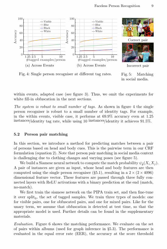
Fig. 6: Person pair matching on the set of pairs in photo albums. The numbersin parentheses are the equal error rates (EER). The “visible unary base” refersto the baseline where only unaries are used to determine match.
where false positive and false negative rates meet. The three obfuscation typemodels are evaluated on the corresponding obfuscation pairs.
Fine-tuning on split0 is crucial. By fine-tuning on the tagged examples of queryidentities, matching performance improves significantly. For the visible pair model,EER improves from 79.1% to 92.7% in the within events setting, and from 74.5%to 81.4% in across events.
Unary baseline. In order to evaluate whether the matching network has learnedto predict match better than its initialisation model, we consider the unary base-line. See “visible unary base” in figure 6. It first compares the unary prediction(argmax) for a given pair, and then determines its confidence using the predictionentropies. See supplementary materials for more detail.
The unary baseline performs marginally better than the visible pair modelunder the within events: 93.7% versus 92.7%. Under the across events, on theother hand, the visible pair model beats the baseline by a large margin: 81.4%versus 67.4% (figure 6). In practice, the system has no information whether thequery image is from within or across events. The system thus uses the pairwisetrained model (visible pair model), which performs better on average.
General comments. The matching network performs better under the withinevents setting than across events, and better for the visible pairs than for mixedor black pairs. See figure 6.
5.3 Graph inference
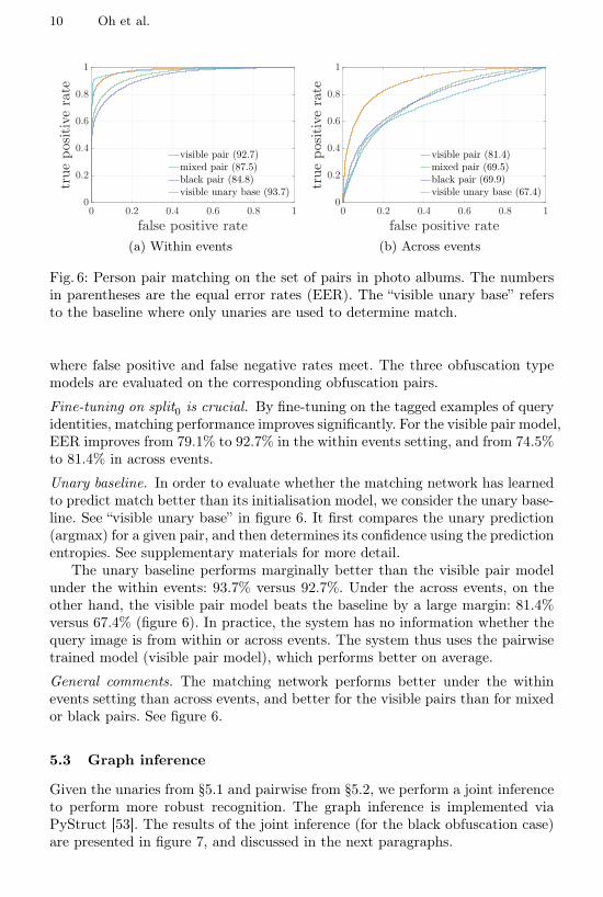
Given the unaries from §5.1 and pairwise from §5.2, we perform a joint inferenceto perform more robust recognition. The graph inference is implemented viaPyStruct [53]. The results of the joint inference (for the black obfuscation case)are presented in figure 7, and discussed in the next paragraphs.
Faceless Person Recognition 11
S1 S2 S3
0
20
40
60
80
100accuracy
(a) Within eventsS1 S2 S3
0
20
40
60
80
100
accuracy
unaryunary+pairwiseunary+pairwise (no pruning)unary+pairwise (oracle)
(b) Across events
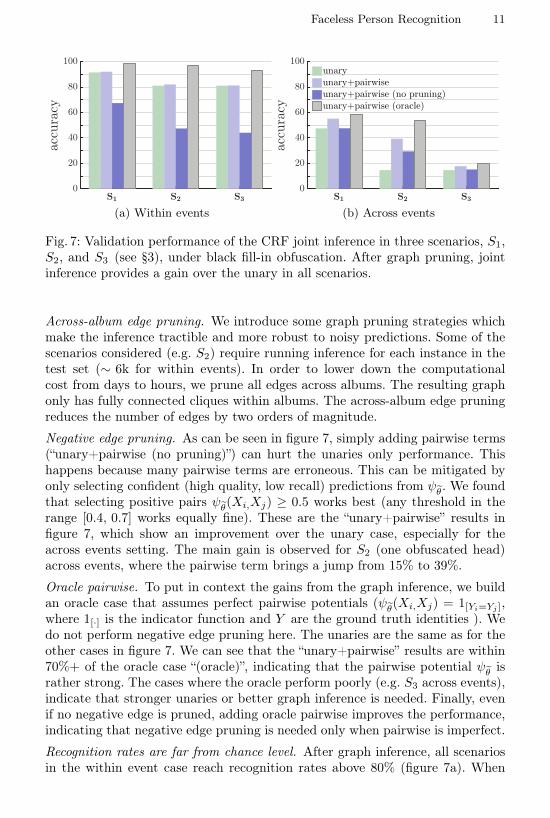
Fig. 7: Validation performance of the CRF joint inference in three scenarios, S1,S2, and S3 (see §3), under black fill-in obfuscation. After graph pruning, jointinference provides a gain over the unary in all scenarios.
Across-album edge pruning. We introduce some graph pruning strategies whichmake the inference tractible and more robust to noisy predictions. Some of thescenarios considered (e.g. S2) require running inference for each instance in thetest set (∼ 6k for within events). In order to lower down the computationalcost from days to hours, we prune all edges across albums. The resulting graphonly has fully connected cliques within albums. The across-album edge pruningreduces the number of edges by two orders of magnitude.
Negative edge pruning. As can be seen in figure 7, simply adding pairwise terms(“unary+pairwise (no pruning)”) can hurt the unaries only performance. Thishappens because many pairwise terms are erroneous. This can be mitigated byonly selecting confident (high quality, low recall) predictions from ψθ. We foundthat selecting positive pairs ψθ(Xi,Xj) ≥ 0.5 works best (any threshold in therange [0.4, 0.7] works equally fine). These are the “unary+pairwise” results infigure 7, which show an improvement over the unary case, especially for theacross events setting. The main gain is observed for S2 (one obfuscated head)across events, where the pairwise term brings a jump from 15% to 39%.
Oracle pairwise. To put in context the gains from the graph inference, we buildan oracle case that assumes perfect pairwise potentials (ψθ(Xi,Xj) = 1[Yi=Yj ],where 1[·] is the indicator function and Y are the ground truth identities ). Wedo not perform negative edge pruning here. The unaries are the same as for theother cases in figure 7. We can see that the “unary+pairwise” results are within70%+ of the oracle case “(oracle)”, indicating that the pairwise potential ψθ israther strong. The cases where the oracle perform poorly (e.g. S3 across events),indicate that stronger unaries or better graph inference is needed. Finally, evenif no negative edge is pruned, adding oracle pairwise improves the performance,indicating that negative edge pruning is needed only when pairwise is imperfect.
Recognition rates are far from chance level. After graph inference, all scenariosin the within event case reach recognition rates above 80% (figure 7a). When
12 Oh et al.
across events, both S1 and S2 are above 35% (figure 7b). These are recognitionfar above the chance level (1%/5% within/across events, shown in figure 3). OnlyS3 (all user heads with black obfuscation) show a dreadful drop in recognitionrate, where neither the unaries nor the pairwise terms bring much help. Seesupplementary materials for more details in this section.
6 Test set results & analysis
Following the experimental protocol in §4, we now evaluate our Faceless Recog-nition System on the PIPA test set. The main results are summarised in figures8 and 9. We observe the same trends as the validation set results discussed in§5. Figure 14 shows some qualitative results over the test set. We organize theresults along the same privacy sensitive dimensions that we defined in §3 in orderto build our study scenarios.
Amount of tagged heads. Figure 8 shows that even with only 1.25 tagged photosper person on average, the system can recognise users far better than chance level(naive baseline; best guess before looking at the image). Even with such littleamount of training data, the system predicts 56.8% of the instances correctlywithin events and 31.9% across events; which is 73× and 16× higher than chancelevel, respectively. We see that even few tags provide a threat for privacy andthus users concerned with their privacy should avoid having (any of) their photostagged.
Obfuscation type. For both scenario S2 and S3, figure 9 (and the results from§5.1) indicates the same privacy protection ranking for the different obfuscationtypes. From higher protection to lower protection, we have Black ≈ White >Blur > Visible. Albeit blurring does provide some protection, the machine learn-ing algorithm still extracts useful information from that region. When our fullFaceless Recognition System is in use, one can see that (figure 9) obfuscationhelps, but only to a limited degree: e.g. 86.4% (S1) to 71.3% (S3) under withinevents and 51.1% (S1) to 23.9% (S3) under across events.
Amount of obfuscation. We cover three scenarios: every head fully visible (S1),only the test head obfuscated (S2), and every head fully obfuscated (S3). Figure 9shows that within events obfuscating either one (S2) or all (S3) heads is not veryeffective, compared to the across events case, where one can see larger drops forS1 → S2 and S2 → S3. Notice that unary performances are identical for S2 andS3 in all settings, but using the full system raises the recognition accuracy for S2
(since seeing the other heads allow to rule-out identities for the obfuscated head).We conclude that within events head obfuscation has only limited effectiveness,across events only blacking out all heads seems truly effective (S3 black).
Domain shift. In all scenarios, the recognition accuracy is significantly worse inthe across events case than within events (about ∼50% drop in accuracy acrossall other dimensions). For a user, it is a better privacy policy to make sure notagged heads exist for the same event, than blacking out all his heads in theevent.

Faceless Person Recognition 13
S1.251 S2.5
1 S51 S10
1
0
20
40
60
80
100accuracy
(a) Within eventsS1.251 S2.5
1 S51 S10
1
0
20
40
60
80
100
accuracy
unary
unary + pairwise
(b) Across events
Fig. 8: Impact of number of tagged examples: S1.251 , S2.51 , S5
1 , and S101 .
(a) Within events (b) Across events
Fig. 9: Co-recognition results for scenarios S101 , S2, and S3 with black fill-in and
Gaussian blur obfuscations (white fill-in match black results).
Fig. 10: Examples of queries in across events setting, not identified using onlytagged (red boxes) samples, but successfully identified by the Faceless Recog-nition System via joint prediction of the query and non-tagged (white boxes)examples. A subset of both tagged and non-tagged examples are shown; thereare ∼ 10 tagged and non-tagged examples originally. Non-tagged examples areordered in the match score against the query (closest match on the left).
14 Oh et al.
7 Discussion & Conclusion
Within the limitation of any study based on public data, we believe the resultspresented here are a fresh view on the capabilities of machine learning to enableperson recognition in social media under adversarial condition. From a privacyperspective, the results presented here should raise concern. We show that, whenusing state of the art techniques, blurring a head has limited effect. We alsoshow that only a handful of tagged heads are enough to enable recognition, evenacross different events (different day, clothes, poses, point of view). In the mostaggressive scenario considered (all user heads blacked-out, tagged images from adifferent event), the recognition accuracy of our system is 12× higher than chancelevel. It is very probable that undisclosed systems similar to the ones describedhere already operate online. We believe it is the responsibility of the computervision community to quantify, and disseminate the privacy implications of theimages users share online. This work is a first step in this direction. We concludeby discussing some future challenges and directions on privacy implications ofsocial visual media.
Lower bound on privacy threat. The current results focused singularly on thephoto content itself and therefore a lower bound of the privacy implication ofposting such photos. It remains as future work to explore an integrated systemthat will also exploit the images’ meta-data (timestamp, geolocation, cameraidentifier, related user comments, etc.). In the context of the era of “selfie” photos,meta-data can be as effective as head tags. Younger users also tend to cross-postacross multiple social media, and make a larger use of video (e.g. Vine). Usingthese data-form will require developing new techniques.
Training and test data bounds. The performance of recent techniques of featurelearning and inference are strongly coupled with the amount of available trainingdata. Person recognition systems like [20, 27, 26] all rely on undisclosed train-ing data in the order of millions of training samples. Similarly, the evaluationof privacy issues in social networks requires access to sensitive data, which isoften not available to the public research community (for good reasons [1]). Theused PIPA dataset [29] serves as good proxy, but has its limitations. It is anemerging challenge to keep representative data in the public domain in order tomodel privacy implications of social media and keep up with the rapidly evolvingtechnology that is enabled by such sources.
From analysing to enabling. In this work, we focus on the analysis aspect ofperson recognition in social media. In the future, one would like to translatesuch analyses to actionable systems that enable users to control their privacywhile still enabling communication via visual media exchanges.
Acknowledgements This research was supported by the German ResearchFoundation (DFG CRC 1223).
Faceless Person Recognition 15
References
1. Narayanan, A., Shmatikov, V.: Myths and fallacies of personally identifiable in-formation. Communications of the ACM (2010)
2. Narayanan, A., Shmatikov, V.: De-anonymizing social networks. In: IEEE Sym-posium on Security and Privacy. (2009)
3. Zheleva, E., Getoor, L.: To join or not to join: the illusion of privacy in socialnetworks with mixed public and private user profiles. In: International conferenceon World wide web. (2009)
4. Mislove, A., Viswanath, B., Gummadi, K.P., Druschel, P.: You are who you know:inferring user profiles in online social networks. In: International conference onWeb search and data mining. (2010)
5. Ahern, S., Eckles, D., Good, N.S., King, S., Naaman, M., Nair, R.: Over-exposed?:privacy patterns and considerations in online and mobile photo sharing. In: Pro-ceedings of the SIGCHI conference on Human factors in computing systems. (2007)
6. Besmer, A., Richter Lipford, H.: Moving beyond untagging: photo privacy in atagged world. In: Proceedings of the SIGCHI Conference on Human Factors inComputing Systems, ACM (2010) 1563–1572
7. Kee, E., Johnson, M.K., Farid, H.: Digital image authentication from jpeg headers.Transactions on Information Forensics and Security 6(3) (2011) 1066–1075
8. Dirik, A.E., Sencar, H.T., Memon, N.: Digital single lens reflex camera identifica-tion from traces of sensor dust. Transactions on Information Forensics and Security(2008)
9. Chen, M., Fridrich, J., Goljan, M., Lukáš, J.: Determining image origin and in-tegrity using sensor noise. Transactions on Information Forensics and Security(2008)
10. Huang, G.B., Ramesh, M., Berg, T., Learned-Miller, E.: Labeled faces in the wild:A database for studying face recognition in unconstrained environments. Technicalreport, UMass (2007)
11. Benfold, B., Reid, I.: Guiding visual surveillance by tracking human attention. In:BMVC. (2009)
12. Bedagkar-Gala, A., Shah, S.K.: A survey of approaches and trends in person re-identification. IVC (2014)
13. Guillaumin, M., Verbeek, J., Schmid, C.: Is that you? metric learning approachesfor face identification. In: ICCV. (2009)
14. Chen, D., Cao, X., Wen, F., Sun, J.: Blessing of dimensionality: High-dimensionalfeature and its efficient compression for face verification. In: CVPR. (2013)
15. Cao, X., Wipf, D., Wen, F., Duan, G.: A practical transfer learning algorithm forface verification. In: ICCV. (2013)
16. Lu, C., Tang, X.: Surpassing human-level face verification performance on lfw withgaussianface. arXiv (2014)
17. Li, W., Wang, X.: Locally aligned feature transforms across views. In: CVPR.(2013)
18. Zhao, R., Ouyang, W., Wang, X.: Person re-identification by salience matching.In: ICCV. (2013)
19. Bak, S., Kumar, R., Bremond, F.: Brownian descriptor: A rich meta-feature forappearance matching. In: WACV. (2014)
20. Taigman, Y., Yang, M., Ranzato, M., Wolf, L.: Deepface: Closing the gap tohuman-level performance in face verification. In: CVPR. (2014)
16 Oh et al.
21. Li, W., Zhao, R., Xiao, T., Wang, X.: Deepreid: Deep filter pairing neural networkfor person re-identification. In: CVPR. (2014)
22. Yi, D., Lei, Z., Li, S.Z.: Deep metric learning for practical person re-identification.ICPR (2014)
23. Hu, Y., Yi, D., Liao, S., Lei, Z., Li, S.: Cross dataset person re-identification. In:ACCV, workshop. (2014)
24. Zhou, E., Cao, Z., Yin, Q.: Naive-deep face recognition: Touching the limit of lfwbenchmark or not? arXiv (2015)
25. Parkhi, O.M., Vedaldi, A., Zisserman, A.: Deep face recognition. BMVC 1(3)(2015) 6
26. Schroff, F., Kalenichenko, D., Philbin, J.: Facenet: A unified embedding for facerecognition and clustering. In: CVPR. (2015)
27. Sun, Y., Wang, X., Tang, X.: Deeply learned face representations are sparse,selective, and robust. In: CVPR. (2015)
28. Gallagher, A., Chen, T.: Clothing cosegmentation for recognizing people. In:CVPR. (2008)
29. Zhang, N., Paluri, M., Taigman, Y., Fergus, R., Bourdev, L.: Beyond frontal faces:Improving person recognition using multiple cues. In: CVPR. (2015)
30. Oh, S.J., Benenson, R., Fritz, M., Schiele, B.: Person recognition in personal photocollections. In: ICCV. (2015)
31. Gong, S., Cristani, M., Yan, S., Loy, C.C.: Person re-identification. Springer (2014)32. Wu, L., Shen, C., van den Hengel, A.: Personnet: Person re-identification with
deep convolutional neural networks. In: arXiv. (2016)33. Cui, J., Wen, F., Xiao, R., Tian, Y., Tang, X.: Easyalbum: an interactive photo
annotation system based on face clustering and re-ranking. In: SIGCHI. (2007)34. Mathialagan, C.S., Gallagher, A.C., Batra, D.: Vip: Finding important people in
images. In: CVPR. (2015)35. Everingham, M., Sivic, J., Zisserman, A.: Hello! my name is... buffy–automatic
naming of characters in tv video. In: BMVC. (2006)36. Everingham, M., Sivic, J., Zisserman, A.: Taking the bite out of automated naming
of characters in tv video. IVC (2009)37. Ding, C., Tao, D.: A comprehensive survey on pose-invariant face recognition.
arXiv (2015)38. Cheng, D.S., Cristani, M., Stoppa, M., Bazzani, L., Murino, V.: Custom pictorial
structures for re-identification. In: BMVC. (2011)39. Gandhi, V., Ronfard, R.: Detecting and naming actors in movies using generative
appearance models. In: CVPR. (2013)40. Kumar, N., Berg, A.C., Belhumeur, P.N., Nayar, S.K.: Attribute and simile clas-
sifiers for face verification. In: CVPR. (2009)41. Layne, R., Hospedales, T.M., Gong, S., Mary, Q.: Person re-identification by at-
tributes. In: BMVC. (2012)42. Gallagher, A.C., Chen, T.: Using group prior to identify people in consumer images.
In: CVPR. (2007)43. Stone, Z., Zickler, T., Darrell, T.: Autotagging facebook: Social network context
improves photo annotation. In: CVPR workshops. (2008)44. Garg, R., Seitz, S.M., Ramanan, D., Snavely, N.: Where’s waldo: matching people
in images of crowds. In: CVPR. (2011)45. Lin, D., Kapoor, A., Hua, G., Baker, S.: Joint people, event, and location recogni-
tion in personal photo collections using cross-domain context. In: ECCV. (2010)46. Shi, J., Liao, R., Jia, J.: Codel: A human co-detection and labeling framework. In:
ICCV. (2013)
Faceless Person Recognition 17
47. Wilber, M.J., Shmatikov, V., Belongie, S.J.: Can we still avoid automatic facedetection? arXiv (2016)
48. Gopalan, R., Taheri, S., Turaga, P., Chellappa, R.: A blur-robust descriptor withapplications to face recognition. PAMI (2012)
49. Punnappurath, A., Rajagopalan, A.N., Taheri, S., Chellappa, R., Seetharaman, G.:Face recognition across non-uniform motion blur, illumination, and pose. Trans-actions on Image Processing (2015)
50. Vu, T., Osokin, A., Laptev, I.: Context-aware CNNs for person head detection.In: International Conference on Computer Vision (ICCV). (2015)
51. Hayder, Z., He, X., Salzmann, M.: Structural kernel learning for large scale mul-ticlass object co-detection. In: 2015 IEEE International Conference on ComputerVision (ICCV), IEEE (2015) 2632–2640
52. Krizhevsky, A., Sutskever, I., Hinton, G.E.: Imagenet classification with deepconvolutional neural networks. In: NIPS. (2012)
53. Müller, A.C., Behnke, S.: pystruct - learning structured prediction in python.Journal of Machine Learning Research 15 (2014) 2055–2060
54. Jia, Y., Shelhamer, E., Donahue, J., Karayev, S., Long, J., Girshick, R., Guadar-rama, S., Darrell, T.: Caffe: Convolutional architecture for fast feature embedding.arXiv (2014)
55. Deng, J., Dong, W., Socher, R., Li, L.J., Li, K., Fei-Fei, L.: ImageNet: A Large-Scale Hierarchical Image Database. In: CVPR. (2009)
Supplementary Materials
A Content
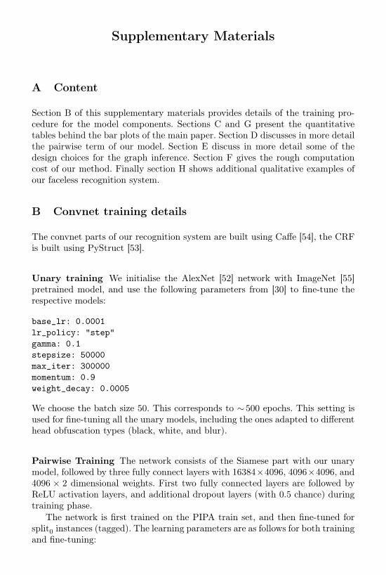
Section B of this supplementary materials provides details of the training pro-cedure for the model components. Sections C and G present the quantitativetables behind the bar plots of the main paper. Section D discusses in more detailthe pairwise term of our model. Section E discuss in more detail some of thedesign choices for the graph inference. Section F gives the rough computationcost of our method. Finally section H shows additional qualitative examples ofour faceless recognition system.
B Convnet training details
The convnet parts of our recognition system are built using Caffe [54], the CRFis built using PyStruct [53].
Unary training We initialise the AlexNet [52] network with ImageNet [55]pretrained model, and use the following parameters from [30] to fine-tune therespective models:
base_lr: 0.0001lr_policy: "step"gamma: 0.1stepsize: 50000max_iter: 300000momentum: 0.9weight_decay: 0.0005
We choose the batch size 50. This corresponds to ∼ 500 epochs. This setting isused for fine-tuning all the unary models, including the ones adapted to differenthead obfuscation types (black, white, and blur).
Pairwise Training The network consists of the Siamese part with our unarymodel, followed by three fully connect layers with 16384×4096, 4096×4096, and4096 × 2 dimensional weights. First two fully connected layers are followed byReLU activation layers, and additional dropout layers (with 0.5 chance) duringtraining phase.
The network is first trained on the PIPA train set, and then fine-tuned forsplit0 instances (tagged). The learning parameters are as follows for both trainingand fine-tuning:

Faceless Person Recognition 19
base_lr: 0.00001lr_policy: "step"gamma: 0.5stepsize: 2000iter_size: 8max_iter: 10000 # 5000 for split0 fine-tuningmomentum: 0.9momentum2: 0.999weight_decay: 0.0000clip_gradients: 10solver_type: ADAM
We choose the batch size of 100 and maintain the same ratio of positive and neg-ative pairs (1 : 9) for each batch. The training pairs consist of the pairs withinPIPA albums because eventually these are the edges used in the graph inference.Depending on the setting (within/across events), 10K training iterations corre-spond to 1∼2 epochs. We stop at 10K training iterations, as the loss does notdecrease further. For fine-tuning, we stop at 5K iterations.

20 Oh et al.
C Unaries recognition accuracy
Tables 2 and 3 show the accuracy of the unary system alone in the presence ofhead obfuscation and with different tag rates, respectively.
Table 2: Impact of head obfuscation on the unary term. Validation set accuracyis shown. (Equivalent to figure 3 in main paper)
Visible Blur Black White NaiveSetting Raw Adapt Raw Adapt Raw Adapt Baseline
Within events 91.5 84.3 86.7 80.1 80.9 78.3 79.6 1.04Across events 47.4 23.5 28.8 14.0 14.7 13.1 13.7 4.65
Table 3: Impact of tag rate on the unary term. Validation set accuracy is shown.(Equivalent to figure 4 in main paper)
Setting Tag rate Visible Blur Black White
Within events
1.25 69.9 63.1 57.3 54.62.5 78.2 71.8 65.0 63.05 83.6 78.0 70.9 69.010 91.5 86.7 80.9 79.6
Across events
1.25 34.9 22.2 11.4 10.92.5 38.5 24.3 12.2 11.25 42.7 24.5 12.0 11.410 47.4 28.8 14.7 13.7
Faceless Person Recognition 21
D Pairwise term
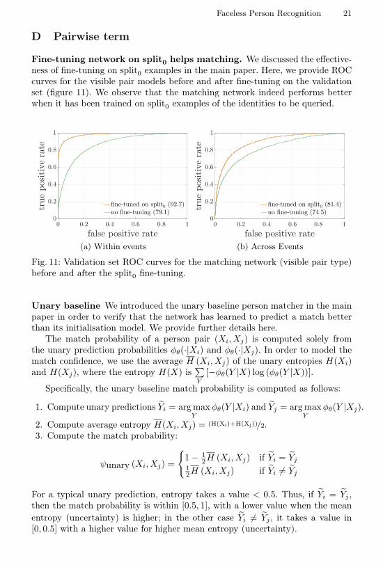
Fine-tuning network on split0 helps matching. We discussed the effective-ness of fine-tuning on split0 examples in the main paper. Here, we provide ROCcurves for the visible pair models before and after fine-tuning on the validationset (figure 11). We observe that the matching network indeed performs betterwhen it has been trained on split0 examples of the identities to be queried.
0 0.2 0.4 0.6 0.8 1
false positive rate
0
0.2
0.4
0.6
0.8
1
truepositiverate
fine-tuned on split0 (92.7)no fine-tuning (79.1)
(a) Within events
0 0.2 0.4 0.6 0.8 1
false positive rate
0
0.2
0.4
0.6
0.8
1
truepositiverate
fine-tuned on split0 (81.4)no fine-tuning (74.5)
(b) Across Events
Fig. 11: Validation set ROC curves for the matching network (visible pair type)before and after the split0 fine-tuning.
Unary baseline We introduced the unary baseline person matcher in the mainpaper in order to verify that the network has learned to predict a match betterthan its initialisation model. We provide further details here.
The match probability of a person pair (Xi, Xj) is computed solely fromthe unary prediction probabilities φθ(·|Xi) and φθ(·|Xj). In order to model thematch confidence, we use the average H (Xi, Xj) of the unary entropies H(Xi)and H(Xj), where the entropy H(X) is
∑Y
[−φθ(Y |X) log (φθ(Y |X))].
Specifically, the unary baseline match probability is computed as follows:
1. Compute unary predictions Yi = argmaxY
φθ(Y |Xi) and Yj = argmaxY
φθ(Y |Xj).
2. Compute average entropy H(Xi, Xj) = (H(Xi)+H(Xj))/2.3. Compute the match probability:
ψunary (Xi, Xj) =
{1− 1
2H (Xi, Xj) if Yi = Yj12H (Xi, Xj) if Yi 6= Yj
For a typical unary prediction, entropy takes a value < 0.5. Thus, if Yi = Yj ,then the match probability is within [0.5, 1], with a lower value when the meanentropy (uncertainty) is higher; in the other case Yi 6= Yj , it takes a value in[0, 0.5] with a higher value for higher mean entropy (uncertainty).

22 Oh et al.
E CRF inference
In this section, we supplement the discussion about the following inference prob-lem in the main paper.
argmaxY
1
|V |∑i∈V
φθ(Yi|Xi) +α
|E|∑
(i, j)∈E
1[Yi=Yj ]ψθ(Xi, Xj). (2)
We describe the effect of changing values of α in §E.1. We then discuss thepruning (§E.2) and approximate inference (§E.3) strategies to realise efficientinference. We include the numerical results for the validation graph inferenceexperiment (figure 7 in the main paper) in §E.4.
E.1 Changing α
We use the unary-pairwise balancing term α = 100 for all the experiments in themain paper, as the performance reaches a plateau for α around 100. In figure 12,we show the performance of the system in three different scenarios (S1, S2, andS3) at different values of α on the validation set. Black obfuscation is used forscenarios S2 and S3. We observe that the plateau is reached at around α = 100for both within and across events cases.
10−3 10−2 10−1 100 101 102 103 104 105
α
0
20
40
60
80
100
accuracy S1 (unary+pairwise)
S2 (unary+pairwise)
S3 (unary+pairwise)
S1 (unary only)
S2 & S3 (unary only)
(a) Within events
10−3 10−2 10−1 100 101 102 103 104 105
α
0
20
40
60
80
100
accuracy
S1 (unary+pairwise)
S2 (unary+pairwise)
S3 (unary+pairwise)
S1 (unary only)
S2 & S3 (unary only)
(b) Across Events
Fig. 12: Effect of α on the inference performance.
E.2 Graph pruning
Inter-album edge pruning As described in the main paper, we prune the fullgraph down by only having fully connected cliques within albums. As shown intable 4, this reduces the number of edges by two orders of magnitude. This alsoallows album-wise parallel computation in a multi-core environment.
Faceless Person Recognition 23
Table 4: Problem size for the graphical models.
Setting Test/Val #classes #nodes #edges (pruned) #albums
Within events Test 581 6 443 20 752 903 (252 431) 351Val 366 4 820 11 613 790 (228 116) 300
Across events Test 199 2 485 3 086 370 (51 633) 192Val 65 1 076 578 350 (17 095) 137
We provide details of the “preliminary oracle experiments” discussed in §5.3of main paper. In order to quantify how much we lose from the pruning, we per-form an oracle experiments assuming perfect propagation (given actual unaries)on the validation set. In the within events case, perfect propagation inside al-bum cliques already gives 98.6%, compared to 99.8% for full graph propagation.Thus, nearly all the information for a perfect inference is already present insideeach album. Under the across events, the oracle numbers are 79.8% (inside al-bum propagation) and 89.2% (full graph propagation). As current unary modelperformance on across events (47.4%) is still far worse than those oracles, wechoose efficiency over the extra 10% boost in the oracle performance.
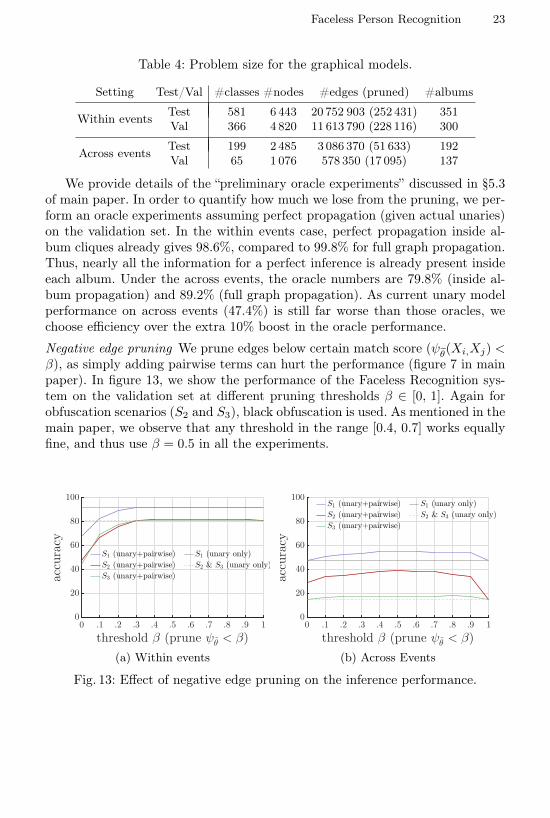
Negative edge pruning We prune edges below certain match score (ψθ(Xi,Xj) <β), as simply adding pairwise terms can hurt the performance (figure 7 in mainpaper). In figure 13, we show the performance of the Faceless Recognition sys-tem on the validation set at different pruning thresholds β ∈ [0, 1]. Again forobfuscation scenarios (S2 and S3), black obfuscation is used. As mentioned in themain paper, we observe that any threshold in the range [0.4, 0.7] works equallyfine, and thus use β = 0.5 in all the experiments.
0 .1 .2 .3 .4 .5 .6 .7 .8 .9 1
threshold β (prune ψθ < β)
0
20
40
60
80
100
accuracy
S1 (unary+pairwise)
S2 (unary+pairwise)
S3 (unary+pairwise)
S1 (unary only)
S2 & S3 (unary only)
(a) Within events
0 .1 .2 .3 .4 .5 .6 .7 .8 .9 1
threshold β (prune ψθ < β)
0
20
40
60
80
100
accuracy
S1 (unary+pairwise)
S2 (unary+pairwise)
S3 (unary+pairwise)
S1 (unary only)
S2 & S3 (unary only)
(b) Across Events
Fig. 13: Effect of negative edge pruning on the inference performance.
24 Oh et al.
E.3 Approximate inference
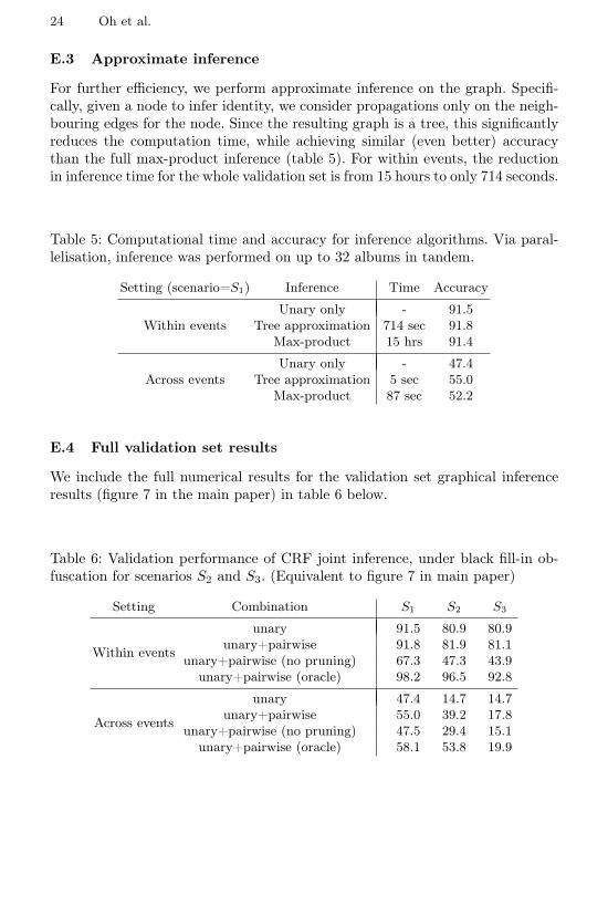
For further efficiency, we perform approximate inference on the graph. Specifi-cally, given a node to infer identity, we consider propagations only on the neigh-bouring edges for the node. Since the resulting graph is a tree, this significantlyreduces the computation time, while achieving similar (even better) accuracythan the full max-product inference (table 5). For within events, the reductionin inference time for the whole validation set is from 15 hours to only 714 seconds.
Table 5: Computational time and accuracy for inference algorithms. Via paral-lelisation, inference was performed on up to 32 albums in tandem.
Setting (scenario=S1) Inference Time Accuracy
Within eventsUnary only - 91.5
Tree approximation 714 sec 91.8Max-product 15 hrs 91.4
Across eventsUnary only - 47.4
Tree approximation 5 sec 55.0Max-product 87 sec 52.2
E.4 Full validation set results
We include the full numerical results for the validation set graphical inferenceresults (figure 7 in the main paper) in table 6 below.
Table 6: Validation performance of CRF joint inference, under black fill-in ob-fuscation for scenarios S2 and S3. (Equivalent to figure 7 in main paper)
Setting Combination S1 S2 S3
Within events
unary 91.5 80.9 80.9unary+pairwise 91.8 81.9 81.1
unary+pairwise (no pruning) 67.3 47.3 43.9unary+pairwise (oracle) 98.2 96.5 92.8
Across events
unary 47.4 14.7 14.7unary+pairwise 55.0 39.2 17.8
unary+pairwise (no pruning) 47.5 29.4 15.1unary+pairwise (oracle) 58.1 53.8 19.9
Faceless Person Recognition 25
F Computation time
For unary convnet training, it takes 1 ∼ 2 days to train on a single GPU ma-chine. Unary logistic regression training takes ∼ 30 minutes. On a single GPU,pairwise matching network training and fine-tuning take ∼ 12 hours and ∼ 6hours, respectively.
Details for graph inference time is found in table 5. Note that before inter-album pruning, inference over the entire test set takes more than several days.However, after pruning and applying the approximate inference, it takes ∼ 5seconds for across events, and ∼10 minutes for within events.
G Test results
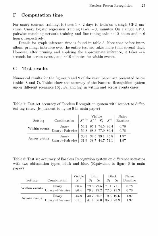
Numerical results for the figures 8 and 9 of the main paper are presented below(tables 8 and 7). Tables show the accuracy of the Faceless Recognition systemunder different scenarios (Sτ1 , S2, and S3) in within and across events cases.
Table 7: Test set accuracy of Faceless Recognition system with respect to differ-ent tag rates. (Equivalent to figure 9 in main paper)
Visible NaiveSetting Combination S1.25
1 S2.51 S5
1 S101 Baseline
Within events Unary 54.2 65.1 74.5 86.4 0.78Unary+Pairwise 56.8 68.3 77.0 86.4 0.78
Across events Unary 30.5 34.5 39.1 45.8 1.97Unary+Pairwise 31.9 38.7 44.7 51.1 1.97
Table 8: Test set accuracy of Faceless Recognition system on difference scenarioswith two obfuscation types, black and blur. (Equivalent to figure 8 in mainpaper)
Visible Blur Black NaiveSetting Combination S10
1 S2 S3 S2 S3 Baseline
Within events Unary 86.4 79.5 79.5 71.1 71.1 0.78Unary+Pairwise 86.4 79.8 79.2 72.6 71.3 0.78
Across events Unary 45.8 30.7 30.7 19.6 19.6 1.97Unary+Pairwise 51.1 41.4 36.0 35.0 23.9 1.97
26 Oh et al.
H Qualitative results
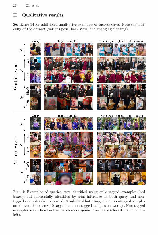
See figure 14 for additional qualitative examples of success cases. Note the diffi-culty of the dataset (various pose, back view, and changing clothing).
Fig. 14: Examples of queries, not identified using only tagged examples (redboxes), but successfully identified by joint inference on both query and non-tagged examples (white boxes). A subset of both tagged and non-tagged samplesare shown; there are ∼10 tagged and non-tagged samples on average. Non-taggedexamples are ordered in the match score against the query (closest match on theleft).